imaging hydraulic fractures: source location …

IMAGING HYDRAULIC FRACTURES: SOURCELOCATION UNCERTAINTY ANALYSIS AT THE

UPRC CARTHAGE TEST SITE

Yingping Li

Earth Resources LaboratoryDepartment of Earth, Atmospheric, and Planetary Sciences

Massachusetts Institute of TechnologyCambridge, MA 02139

Xianhuai -Zhu

Union Pacific ResourcesFort Worth, TX 76101

Arthur C. H. Cheng, and M. Nafi Toksoz

Earth Resources LaboratoryDepartment of Earth, Atmospheric, and Planetary Sciences

Massachusetts Institute of TechnologyCambridge, MA 02139

ABSTRACT

Hydraulic fracturing is a useful tool for enhancing gas and oil production. Highresolution seismic imaging of the fracture geometry and fracture growth process is thekey in determining optimal spacing and location of wells and in improving reservoir performance for increased production rate. In this paper, we address how accurately thesources along a fracture zone at different depths can be determined for given velocitymodels, geophone array geometry configurations, and location of monitor wells. We apply a theory of uncertainty analysis to estimate microearthquake location uncertaintiesin both relative and absolute senses. To estimate the location uncertainties, we usedthe velocity models, two geophone arrays in two monitor wells, and the location of thefracture well, and an assumed fracture orientation of an upcoming hydraulic fracturingexperiment by Union Pacific Resources Company (UPRC) and its partners at Carthage

15-1

Li et al.

Field, Panola, Texas.We calculated the 95% confidence regions, in both absolute and relative senses, for

five hypothetical sources along an assumed strike of a target fracture zone at threedifferent depths. The semimajor and semiminor axes of the relative error ellipses forthese epicenters are typically estimated to be 12 and 5 ft, respectively, and the relativedepth uncertainty is derived at about 6 ft. The absolute location uncertainties are atleast 3 to 10 times larger than the relative location uncertainties. The high-precisionrelative source locations result in a relative measurement error about 4-15% in measuringthe fracture length. The location ambiguity from two-station locations is discussed andarrival azimuthals is proposed to to be used for removing such location ambiguity.The location uncertainty analysis is expected to be generalized as a practical tool inoptimal designing of a two-well seismic monitoring system for high-resolution imagingof hydraulic fractures.

INTRODUCTION

Hydraulic fracturing has been a common engineering practice in the enhancement of gasand oil production, geothermal energy extraction, and the safe disposal of hazardouswaste (Fehler et aI., 1987; Vinegar et aI., 1992; Truby et al., 1994; Li et al., 1995a,1996). Understanding the fracture process and geometry is very important in designinga hydraulic fracture treatment for optimizing production efficiency from a hydrocarbonreservoir (Wills et al., 1992; Zhu et al., 1996). The knowledge of fracture orientation,height, and extent is essential to determine the optimal spacing and location of wells andwill result in better reservoir performance in the case of both primary and secondaryproduction.

Hydraulic fracturing often induces microearthquakes in a hydraulic fracture zoneand its vicinity. Seismic monitoring techniques have been used to image the fracturegeometry (House, 1987; Wills et aI., 1992; Phillips et al., 1992; Block et al., 1993; Li etal., 1995a, 1996) and to reveal the fracture growth process (Li et al., 1995a, 1996). Theseismic imaging technique has proven to be one of the best methods for 3-D imaging andcharacterizing subsurface fractures and cracks. Seismic monitoring techniques trace thefracture growth process in real time and estimate the hypocentral locations of inducedmicroearthquakes and associated location uncertainties. Microearthquakes induced byhydraulic fracturing at the Fenton Hill geothermal test site were located with an absolutelocation error of 30 to 40 meters (House, 1987; Phillips et aI., 1992; Li et al., 1995a, 1996)and a relative location uncertainty of about 5 meters (Phillips et aI., 1992; Li et aI.,1995a, 1996) using seismic data recorded at four borehole stations. Vinegar et al. (1992)estimated the accuracy of relative location for microearthquakes induced by hydraulicfracturing in the Belridge diatomite to be less than ± 5 ft with four seismic arrays inthree monitor wells. Rieven and Rodi (1995) estimated the best relative location errorsto be about 3 to 8 ft for induced microearthquakes at the test site for the Deep WellTreatment and Injection (DWTI) program in Jasper, Texas, with seismic data from 96

15-2

Imaging Hydraulic Fractures: UPRC Carthage Test Site

of the 150 available geophones in two monitor wells.To obtain a better understanding of. the fracture geometry and fracture growth

process in the Cotton Valley tight gas sands, Union Pacific Resources Company (UPRC)carried out a pilot study in 1994 to detect and locate microearthquakes induced byhydraulic fracturing in the Carthage Field, Panola County, Texas (Zhu et al., 1996).Seismic events induced by hydraulic fracturing at a depth of 9500 ft were detectable ata distance exceeding 1300 ft in Carthage's sand and shale formations (Zhu et al., 1996).Following this pilot test, a massive hydraulic fracturing experiment was proposed to becarried out at Carthage Field in 1996. One of the major goals of this experiment is toimage the fracture geometry and growth process with seismic waveforms generated bymicroearthquakes induced by hydraulic fracturing.

In order to reliably and accurately estimate the fracture length, azimuth, and heightusing the high-precision source location of induced earthquakes, it is critical to analyze location errors for a given source-receiver geometry configuration. Location erroranalysis has been widely used in earthquake seismology for the optimal designing ofseismic networks (Kijko, 1977; Uhrhammer,1980; Lee and Stewart, 1981), and forevaluating the performance of a sparse regional network (Li and Thurber, 1991). Unfortunately, this method has little application in monitoring hydraulic fractures untilrecently. Rieven and Rodi (1995) used a method similar to that of Li and Thurber(1991) to systematically analyze location errors for earthquakes induced by hydraulicfracturing at ARCO's WDTI test site following this experiment. However, to best ofour knowledge, no location error analysis has been done prior to a fracture experimentto obtain insight how the geometry effects on location accuracies. In this study, wewill analyze location ambiguity and location uncertainties, in both absolute and relative senses, for a given velocity model and source-receiver configuration in an upcomingUPRC hydrofracturing experiment and provide some recommendations and suggestionsin advance. Furthermore, our results suggest that the location uncertainty analysis canbe developed as a practical tool for optimally designing a seismic monitoring system forimaging fractures with two monitoring wells.

PRINCIPLES OF LOCATION ERROR ANALYSIS

In a seismic event location problem, we are concerned with an inversion problem forsolving the condition equations:

Ax = d, (1)

where A is an m x 4 matrix of partial derivatives, x is a vector of four unknownhypocentral parameters, and d is the vector of m observed traveltime data. Elementsin three of the four columns of the Jacobian matrix A are spatial partial derivatives oftraveltimes. These derivatives can also be expressed in terms of velocity at a source pointand the direction cosines of ray paths from the source to receivers (Lee and Stewart,1981). Therefore, matrix A can be constructed easily as long as the velocity at thesource and the ray paths are known.

15-3

Li et al.

Since earthquakes are located with a velocity model and arrival time data thatcontain errors, the resulting location and origin. time also contain errors. Since thelocation and origin time are found using generalized inversion, the issue is how thisoperation causes errors in the data to affect the uncertainty of the solution. It is wellknown that if matrix A is ill-conditioned, the solution of x will have a larger uncertainty,and if matrix A is well-conditioned, the solution of x will have a smaller location error.Therefore, matrix A inherently contains information about the location capability for agiven source-receiver geometry. Using the singular-value decomposition (SVD) theorem(Lawson and Hanson, 1974), matrix A can be decomposed into:

A=USyT, (2)

where U is an m x 4 matrix of an orthogonal singular vector associated with the observeddata d, Y is a 4 x 4 matrix of an orthogonal singular vector associated with unknownhypocentral parameters x, and S is a 4 x 4 diagonal matrix of singular values of A. Theratio of the largest to the smallest singular value is defined as the condition numberof A, which is an upper bound in magnifying the -traveltime errors to the locationuncertainties.

Assuming variances (cr) of traveltime data are equal and independent for each observed datum, the covariance matrix C for the parameter space is

C = YS-2yTcr2 . (3)

The elements of the diagonal of matrix C are estimates of uncertainties in the unknownhypocentral parameters. We can derive the origin time and the focal depth uncertaintyas well as the epicentral error ellipse from matrix C, as long as the velocity model,source-receiver geometry, and traveltime data variances are known.

In earthquake location problems, a velocity model is of critical importance for calculating the ray paths and traveltimes of seismic waves passing through the ray paths.There are two major error sources for locating an earthquake: One is from an incorrect velocity model used for location, the other is the measurement error for the arrivaltimes of seismic phases at receivers. The incorrect velocity model will bias the absolutelocation of an event significantly, but has less of an effect on the relative location of twoor more events very close to each other (Jordan and Sverdrup, 1981, Rodi et al., 1993),since the systematic error caused by an incorrect velocity model can be eliminated orreduced by using station corrections. This is the basic idea of Joint Hypocenter Determination (JHD) (Douglas, 1967). The second type of error-the reading error of arrivaltimes-can be significantly reduced by using waveform correlation analysis (Poupinetet al., 1984; Phillips et al., 1992; Moriya et al., 1994; Li et al., 1995a,b). This kind oferror mainly affects the accuracy of relative source locations among a cluster of seismicevents. Therefore, we can obtain high-precision relative event locations by using bothJHD idea and waveform correlation analysis.

In the practice of earthquake location, if arrival time data at multiple stations areavailable, we can estimate the origin times and hypocentral locations for a group of

15-4


seismic events based on traveltimes calculated with a given velocity model. The misfits between theoretical traveltimes and observed data are traveltime residuals. Thetraveltime residuals contain the contribution from both the velocity model errors andthe reading errors of the arrival times of seismic phases. We can roughly separate thevelocity model error by statistically analyzing the common part of the traveltime residuals for a cluster of seismic events at each station and then correct it with a stationcorrection model. After the station correction is applied, the rest of the residuals aredominated by the reading errors and random errors.

The objective of this study is to assess the uncertainties of earthquake locations inboth absolute and relative senses. The major purpose of the UPRC fracturing projectis to estimate the fracture azimuth, length, and height. Therefore, the accuracies ofrelative source locations will be our major concern. For comparison, we also derived theabsolute location uncertainties based on given velocity models. We will calculate the95% confidence regions for five hypothetical seismic sources along an expected fracturezone in three different layers at the UPRC fracturing test site.

UPRC HYDROFRACTURING EXPERIMENTS AT CARTHAGEFIELD

The UPRC hydrofracturing experiment site is located at Carthage Field, Panola County,Texas. Carthage Field, discovered in 1968, is a thickly layered, low permeability gasreservoir. It is currently experiencing a fourth active drilling period with numerous wellsdrilled in 80-acre spacing. The major geological units in the Carthage gas field are aseries of sand/shale formations. One of the most important production regions is calledthe Cotton Valley.

To better characterize the fractures in the Cotton Valley, UPRC carried out a pilotexperiment to detect microearthquakes in the Carthage Field in May 1994, with fracturetreatment at a depth of 9508 ft, and a three-component geophone in a monitor well ata depth of 9025 ft, and a three-component geophone at the surface. Eighteen seismicevents induced by hydrofracturing were detectable and located by the borehole geophoneat distances exceeding 1300 ft in Carthage's sand and shale formations, where themonitor well was offset significantly from the fracture plane. Following this successfulpilot test, a massive hydraulic fracturing experiment was planned at Carthage Field for1996.

A schematic of configuration for a treatment well (#21-10) and two monitor wells(#21-9 and #22-9) to be used in a massive fracture experiment in the Carthage Field isshown in Figure 1. The horizontal distances from the fracture treatment well (F01) totwo monitor wells, (MOl and M02), are 1257 and 1080 ft, respectively (Figure 2). Thedashed line in Figure 2 indicates an assumed azimuth of an expected hydraulic fracturezone. The expected fracture orientation is assumed along a strike of about N700 E basedon geological information and downhole stress measurement. UPRC's pilot study (Zhuet aI., 1996) roughly estimated that the fracture has an orientation of about N65° E and

15-5

=-- .~

Li et al.

a half-length of 600 to 800 ft.Figure 3 shows a schematic of the geophone arrays in the two monitor wells to be

used for the proposed hydrofracturing project. Monitor wells MOl and M02 will beequipped with 47 and 49 three-component geophones with 50-ft spacing, respectively.288 signal channels will be used to record seismic signals generated by the inducedmicroearthquakes, with a sampling rate of at least 1000 samples per second. Geophonesin well MOl span a depth range of 7650 to 9950 ft and the seismometers in well M02have a depth range of 7650 to 10050 ft (Figure 3). The fracture treatments will beconducted at fracture well (F01) in three different layers: (1) Upper Cotton Valley, (2)Middle Cotton Valley, and (3) Taylor. The center of each layer is located at 8450, 9050,and 9750 ft, respectively. We refer to them as layer 1, 2 and 3, respectively, throughoutthis paper.

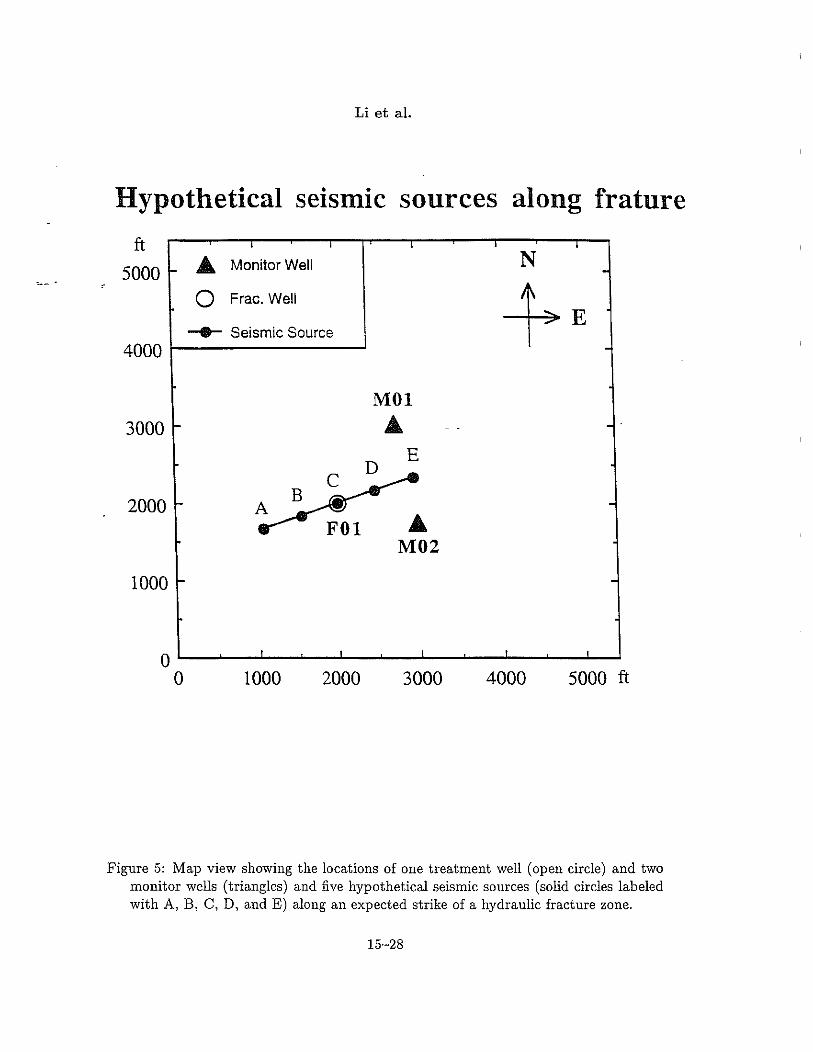
Figure 4 shows a linear gradient velocity model for P- and S-waves for the Carthageexperiment site. This P-wave velocity model was developed based on the sonic well log.The S-wave velocity model was estimated using Castagna's Vp/Vs relation (Castagna,1993). In our error analysis for seismic source locations, we will use this linear gradientvelocity model to calculate ray paths, traveltimes, and partial derivatives of the seismicrays and to construct matrix A in equation (1). To access the spatial variation ofthe source location uncertainties for a given geometry of geophone arrays, we selectedfive hypothetical sources (events A, B, C, D, and E) along the assumed strike of theexpected fracture zone (Figure 5). The five hypothetical sources are evenly distributedalong the expected strike of a fracture zone with the middle event (source C) situatingwithin the treatment well (F01). The distances between these hypothetical sources are500 ft. In the following sections, we start with the analysis of the location ambiguitycaused by two-station locations, and then calculate 95% confidence regions for the fivehypothetical sources in both absolute and relative senses.

LOCATION AMBIGUITY WITH TWO VERTICAL ARRAYS

There will be only one vertical array in each of the two monitor wells in the UPRCmassive fracturing experiment. Locating epicenters of induced earthquakes with twovertical arrays is equivalent to a two-station location problem. It is well-known thatwithout azimuthal information, there is a fundamental ambiguity in the source location:two points located symmetrically about the line connecting two observing stations willalways fit the arrival time data equally well (Li and Thurber, 1991). Rieven and Rodi(1995) found this kind of location ambiguity using only arrival time data from two arraysin the two monitor wells of ARCO's WDTI experiment.

Using the proposed seismic array configuration in the upcoming UPRC fracturingexperiment, we calculated ambiguity locations (A', B', C', D' and E') for five hypothetical sources (A, B, C, D, and E) along the expected strike of the fracture zone at theCarthage test site. We call these ambiguity locations of hypothetical seismic sourcesghost images of the real hypothetical sources. Figure 6 shows the locations of five hy-

15-6


pothetical sources and their ghost images as well as the locations of two arrays in twomonitor wells (MOl and M02) used for locating the sources. The five hypothetic sourcesspan a distance range of 2000 ft along an assumed strike of the expected fracture zone.

Figure 6 clearly shows the location ambiguity with the two vertical arrays in thetwo monitor wells. The effects of this ambiguity to the source locations are two-fold.First, events within the target fracture zone may be located at the locations of theirghost images, rE,sulting in significant uncertainties in estimating the fracture length andorientation. For example, if five real hypothetical sources are all 'mistakenly' locatedat the locations of theic ghost images, then the orientation of the fracture zone will beestimated at about N900 E rather than N70° E. Second, a real seismic source situatedat the region where the five ghost images are located may be mistakenly located withinthe fracture zone. The location ambiguity effects will be even worse if there is scatteredbackground seismicity associated with neighboring production wells which were fractured previously, as shown by Zhu et al. (1996). In order to obtain reliable and accurateestimates of the fracture orientation and length, we have to remove or at least reducesuch an ambiguity effect.

The simplest approach to overcome this kind of location ambiguity problem is touse three or more stations (monitor wells) at different azimuths. For example, Willset ai. (1992) used four arrays in three monitor wells, and House (1987), Phillips etal. (1992), and Li et al. (1995a) used four borehole stations to locate the induced microearthquakes. However, increasing the number of monitor wells will increase the costof the experiment tremendously and may not be feasible for the planned UPRC massivehydrofracturing experiment. Adding a few stations at the surface could be possible andcheaper solution. However, a three-component geophone at the surface deployed duringa pilot study at UPRC's Carthage test site observed no seismic signals from the deephydraulic fracturing, since the fractures may be too deep to be recorded at the surface(Zhu et ai., 1996).

An alternative and feasible way to remove such location ambiguity is to make use ofthe arrival azimuth data along with the arrival time data (Li and Thurber, 1991), sinceazimuth data provide directional information. Li and Thurber (1991) demonstrated theimportance of azimuthal data in locating earthquakes using a sparse network. For thecase of two-station locations, arrival azimuths, estimated from the particle motion ofP-waves at observing stations (e.g., Magotra et ai., 1987; Thurber et aI., 1989), cannotonly readily remove the location ambiguity but also reduce the error ellipses of epicenterlocations (Li and Thurber, 1991). Arrival azimuthal information is obviously the keyto the single-station location (Bratt and Bache, 1988; Li and Thurber, 1991), sincearrival time data from multiple seismic phases at a single station alone can reliablydetermine the distance range but provide no information on direction. However, atheoretical analysis of the single-station location problem by Li and Thurber (1991)indicated that the epicenter constraint will always be relatively weak due to the relativeinaccuracy of arrival azimuth estimation (generally 5 to 100 uncertainty). Zhu et ai.(1996) used both the arrival time and azimuth data from a downhole, three-component

15-7

Li et al.

geophone to estimate epicentral locations for 18 microearthquakes recorded during thepilot fracturing experiment at the Carthage test site. Arrival time and azimuth errorsare estimated to be about 16 ms and 5°, respectively, and the semimajor and semiminoraxes of the error ellipses for epicenters are 400 and 150 ft, respectively.

Although arrival azimuth information will help to remove the location ambiguityfrom two-station locations, an accurate estimate of the arrival azimuth is not an easytask. The major technical difficulty is how to accurately determine the orientationsof the horizontal geophones in deploying the geophone arrays in the deep boreholes.One approach to obtain a reliable estimate of the arrival azimuths is to make use ofboth calibration shots near the surface and downhole implosive sources in a crossholesurvey. We recommend using calibration events along the target fracture zone and inthe region where the ghost images are situated. Horizontal-component waveforms of thecalibration events with known locations can be used to accurately and reliably determinethe orientations of horizontal components of the downhole geophones. The secondaryadvantage of calibration events with known origin times is to provide information aboutthe effects of velocity model uncertainties which call .be used in a station correctionmodel.

From Figure 6 we also note that the location ambiguity effect is different for hypothetical sources at different positions along the assumed fracture. For hypotheticalevents A, B, C, and D, their ghost images are significantly separated from their reallocations. Therefore, adding arrival azimuthal data can immediately remove such location ambiguity. However, the hypothetical event E is too close to its ghost image.Adding azimuth information cannot easily distinguish events E and E' since the azimuthitself has the measurement error of 5° to 10°. Based on this analysis, we can conclude,without doing calculations for error ellipses, that the location uncertainties for eventsclose to sources E and E' will be significantly larger than those for events close to theother four hypothetical sources.

VELOCITY MODEL AND TRAVELTIME RESIDUAL

To estimate source location uncertainties with the SVD method, we need traveltimedata variances to calculate the location errors with equation (3). How to access the datavariances for traveltimes is addressed in this section. In earthquake location practice,data variances of traveltimes due to uncertainties of a velocity model and reading errorsof arrival times are typically estimated by comparing the residuals between the observedand theoretically calculated (with a given model) traveltimes at multiple observingstations. The root-mean-squared (RMS) residuals of traveltimes are typically used asindicators for the location uncertainties. For a cluster of events close to each other, theRMS residuals calculated with multiple stations can be obtained. We can obtain datavariances of traveltimes by statistically analyzing the multiple-station and multipleevent RMS residual data.

Since no multiple-event and multiple-station arrival time data are available yet at

15-8


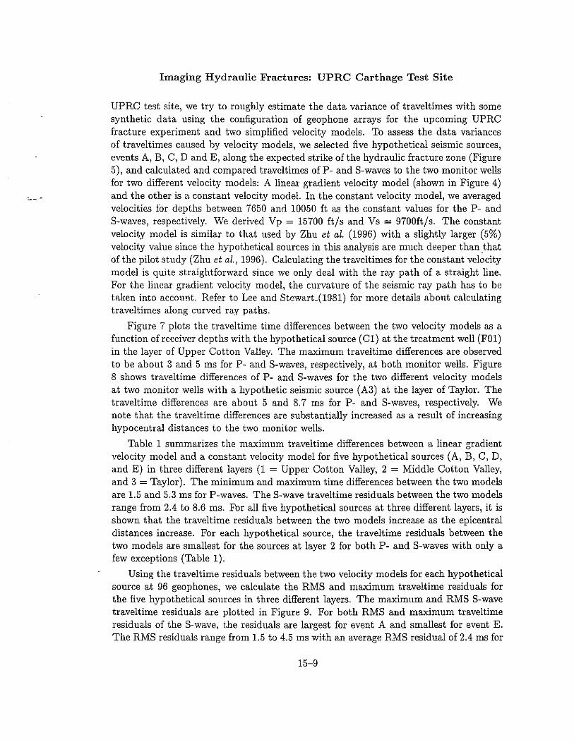
UPRC test site, we try to roughly estimate the data variance of traveltimes with somesynthetic data using the configuration of geophone arrays for the upcoming UPRCfracture experiment and two simplified velocity models. To assess the data variancesof traveltimes caused by velocity models, we selected five hypothetical seismic sources,events A, B, C, D and E, along the expected strike of the hydraulic fracture zone (Figure5), and calculated and compared traveltimes of P- and S-waves to the two monitor wellsfor two different velocity models: A linear gradient velocity model (shown in Figure 4)and the other is a constant velocity model. In the constant velocity model, we averagedvelocities for depths between 7650 and 10050 ft as the constant values for the P- andS-waves, respectively. We derived Vp = 15700 ftls and Vs = 9700ft/s. The constantvelocity model is similar to that used by Zhu et al. (1996) with a slightly larger (5%)velocity value since the hypothetical sources in this analysis are much deeper than thatofthe pilot study (Zhu et al., 1996). Calculating the traveltimes for the constant velocitymodel is quite straightforward since we only deal with the ray path of a straight line.For the linear gradient velocity model, the curvature of the seismic ray path has to betaken into account. Refer to Lee and Stewart_(1981) for more details about calculatingtraveltimes along curved ray paths.

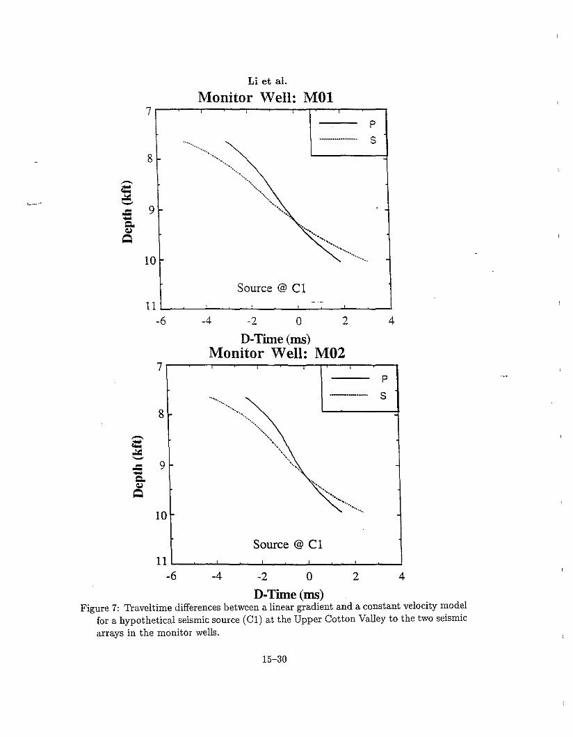
Figure 7 plots the traveltime time differences between the two velocity models as afunction of receiver depths with the hypothetical source (CI) at the treatment well (FOI)in the layer of Upper Cotton Valley. The maximum traveltime differences are observedto be about 3 and 5 ms for P- and S-waves, respectively, at both monitor wells. Figure8 shows traveltime differences of P- and S-waves for the two different velocity modelsat two monitor wells with a hypothetic seismic source (A3) at the layer of Taylor. Thetraveltime differences are about 5 and 8.7 ms for P- and S-waves, respectively. Wenote that the traveltime differences are substantially increased as a result of increasinghypocentral distances to the two monitor wells.

Table I summarizes the maximum traveltime differences between a linear gradientvelocity model and a constant velocity model for five hypothetical sources (A, B, C, D,and E) in three different layers (1 = Upper Cotton Valley, 2 = Middle Cotton Valley,and 3 = Taylor). The minimum and maximum time differences between the two modelsare 1.5 and 5.3 ms for P-waves. The S-wave traveltime residuals between the two modelsrange from 2.4 to 8.6 ms. For all five hypothetical sources at three different layers, it isshown that the traveltime residuals between the two models increase as the epicentraldistances increase. For each hypothetical source, the traveltime residuals between thetwo models are smallest for the sources at layer 2 for both P- and S-waves with only afew exceptions (Table 1).

Using the traveltime residuals between the two velocity models for each hypotheticalsource at 96 geophones, we calculate the RMS and maximum traveltime residuals forthe five hypothetical sources in three different layers. The maximum and RMS S-wavetraveltime residuals are plotted in Figure 9. For both RMS and maximum traveltimeresiduals of the S-wave, the residuals are largest for event A and smallest for event E.The RMS residuals range from 1.5 to 4.5 ms with an average RMS residual of 2.4 ms for

15-9

Li et al.

Table 1: Average Traveltime Residuals at Each Station

Source MOl M02Location P (ms) S(ms) P(ms) S(ms)

Al 4.55 7.37 4.11 6.66A2 3.94 6.38 3.25 5.27A3 5.34 8.56 4.50 7.29B1 3.72 6.11 3.28 5.32B2 3.24 5.25 2.61 4.23B3 4.21 6.92 3.40 5.51C1 2.96 4.80 2.56 4.15C2 2.64 4.27 2.14 3.46C3 3.15 5.11 2.39 3.81D1 2.38 3.85 2.07 3.35D2 2.19 3.55 1.92 3.12D3 2.28 3.69 1.61 2.60E1 2.12 3.43 1.99 3.23E2 2.00 3.24 1.89 3.07E3 1.86 3.01 1.47 2.38

the 15 hypothetical sources. The maximum residuals are 3.0 to 8.7 ms with an averagevalue of 5 ms. Figure 9 also shows typical traveltime errors derived from the pilot studywith data from a single three-component geophone and 18 microearthquakes (Zhu etaI., 1996).

Li et al. (1995a) found an average absolute RMS residual of 4 to 5 ms for 157induced microearthquakes in a hard formation in Fenton Hill, New Mexico. Rievenand Rodi (1995) obtained an average RMS residual of 6 ms for induced earthquakesin a soft formation in Jasper, Texas. The average RMS value we estimated for theUPRC test site with the simplified velocity models is smaller by factors of 2 to 3 thanthose obtained from the other location practices for induced earthquakes. However, ouraverage maximum residual is comparable to these typical RMS residuals from otherlocation practices. Therefore, we believe that our RMS estimates may underestimatethe real traveltime residuals due to our two velocity models being significantly simplied.Our maximum residuals may better represent the typical errors of traveltimes. Zhu etal. (1996) obtained a typical traveltime error of about 16 ms. We believe that this valuemay represent a maximum bound of the traveltime errors.

Based upon the analysis of traveltime residuals for synthetic and real data at theUPRC fracturing test site, we specified two standard deviation models: (1) constant f7

and (2) variable f7 models. In the constant f7 model, we assume f7 = 10 ms for all eventsalong the expected fracture zone. This is a conservative estimation since the value isabout two times larger than the average maximum traveltime residual we derived usingsynthetic data. If we take into account the effects from the lateral heterogeneity of

15-10

=-- ,~


the real earth structure, sharp interfaces and anisotropy in the propagation medium,the large standard deviation value in the Gonstant model is even more reasonable. Thismodel provides an upper bound of estimates for absolute uncertainties in the traveltimes.The variable (f model takes the spatial variation (Figure 9) of traveltime residuals intoaccount. In the variable (f model, we use the S-wave maximum traveltime residuals forfive hypothetical sources in layer 2 (Table 1 and Figure 9) as the standard deviation foreach corresponding hypothetical source. This model provides a lower bound of estimatesfor absolute uncertainties in the traveltimes.

ABSOLUTE SOURCE LOCATION UNCERTAINTIES

So far, we have discussed the basic principle for estimating source location uncertaintiesin both absolute and relative senses using the SVD method. In this section, we estimatethe absolute location uncertainties for hypothetical microearthquake sources in UPRC'shydrofracturing test site at Carthage Field, Panola, Texas, using a linear gradient velocity model (Figure 4) and 96 three-compol1ep.t geophones of two arrays that will bedeployed into two monitor wells (Figure 3).

To estimate the uncertainties of source locations, we need to compute the ray paths,traveltimes between a source and a set of geophone arrays along the ray paths, andthe corresponding spatial derivatives evaluated at the source using a given velocitymodel and the geometry configuration of geophone arrays. For a linear gradient velocitymodel, we deal with the curvatured ray paths from a source to the geophone receivers.The direction cosines of the seismic rays are the cosines of the direction angles whichare defined with respect to the positive direction of the coordinate axes. The spatialderivatives of the traveltimes c'n be expressed in terms of the velocity at the source pointand the direction cosines of the ray paths from the source to the receivers. Therefore,it is easy to construct matrix A in equation (1), using direction cosines of the seismicrays and the velocity at the source. With an SVD method (equation 2) and standarddeviation models as variances of traveltime data, we will construct the covariance matrix(equation 3) and estimate the source location uncertainties, including the epicentralerror ellipse and depth uncertainty.

Location Uncertainties: Constant Vs. Variable (f Models

First, we calculated the absolute location error ellipsoids (95% confidence regions) for thefive hypothetical sources and their ghost images in layer 2 (Middle Cotton Valley) usingthe constant (f model ((f = 10 ms). Figure 10 is a map view showing error ellipses forthese hypothetical sources and their ghost images at layer 2. A striking feature of Figure10 is the extremely large error ellipses for the hypothetical source E and its ghost imageE', as we expected previously from the analysis of the location ambiguity. The strike ofthe semimajor axis of the error ellipse ranges from N71 0 E to N800 E for hypotheticalsources from E to A. For their ghost images E' to A', the strike of the semimajor axis ofthe error ellipse is from N79° E to N87° E. The semimajor axis (a) of the error ellipse

15-11

Li et al.

increases when the hypothetical source moves from A to E. The semimajor axes oferror ellipses at sources A and E are about 80 ft, and 580 ft, respectively. Significantvariation of the semimajor axis will occur for events close to the hypothetical source E.From source A to E, the semiminor axis decreases from 57 to 23 ft. Since a constant (]'model is used, the significant spatial variation of the epicenter error ellipses (Figure 10)can only be attributed to the station-receiver configuration geometry, which significantlyamplifies the traveltime errors to the location uncertainties. We believe that the absolutelocation uncertainties derived based on the constant (]' model represent an upper boundof estimates for absolute location errors.

Second, we calculated the absolute location uncertainties (95% confidence regions)for the five hypothetical sources and their ghost images in layer 2 (Middle CottonValley) with the variable (]' model ((]' = 3.5 to 6.5 ms). Figure 11 plots the epicentererror ellipses for the hypothetical sources A to E and their ghost images A' to E'. Thesemimajor axis (a) for source A to E varies from 39 to 212 ft. The semiminor axis(b) for sources A to E decreases from 37 ft to 8 ft. As one can see from Figure 11,the semimajor axes of the error ellipses for sources A to E, especially for source'E, aresignificantly reduced compared to the results from the constant (]' model (Figure 10).We attribute this significant improvement to a fact that the spatial variation of thetraveltime residuals have been taken into account. However, the semimajor axis (a) ofthe error ellipse for the source E is still quite large. The absolute location errors derivedfrom the variable (]' model can be assumed as a lower bound of estimates for the absolutelocation uncertainty.

The depth uncertainties of five hypothetical sources in layer 2 (Middle Cotton Valley)are calculated with both constant and variable (]' models and are compared in Figure12. The depth uncertainties estimated with both (]' models show the same trend: thedepth uncertainty increases as the epicentral distance between the source and geophonearrays increases (from source E to A). For the constant (]' model, the depth uncertaintyranges from 27.4 to 55.2 ft. The depth uncertainty estimated with the variable (]' modelvaries from 9.4 ft at source E and 35.3 ft at source A.

Figure 13 shows the semiminor axes (b) of epicenter error ellipses calculated withboth constant and variable (]' models for the five hypothetical sources at layer 2. Fromsource A to E, the semiminor axes estimated with both models monotonously decreaseas the epicentral distances decrease. The smallest and largest semiminor axis obtainedwith the constant (]' model are 22.5 ft at source E and 57.3 ft at source A, respectively.The minimum and maximum semiminor axes are estimated to be 7.7 and 36.7 ft, respectively, using the variable (]' model. From Figures 12 and 13, we find that bothdepth uncertainties and semiminor axes (b) derived with a variable (]' model are smallerthan those estimated using the constant (]' model by factors of 1.5 to 3 for the fivehypothetical sources, from A to E.

Using both constant and variable (]' models, we also calculated and compared thesemimajor axes (a) of epicentral error ellipses for five hypothetical sources at layer 2.The spatial variation trend of the semimajor axes (Figure 14) are different from those of

15-12


the depth uncertainty and the semiminor axis (Figures 12 and 13). For the constant (J

model, the semimajor axis increases as the epicentral distances between the source andreceivers decrease (form source A to E). The semimajor axis of the epicenter error ellipsedramatically jumps to 619.2 ft at the hypothetical source E. The large semimajor axisat source E is about 5 times larger than at source D (129.9 ft) and 8 times larger thanat source A (80.1 ft). This indicates that the source-receiver geometry configurationsignificantly amplifies the traveltime errors to the location uncertainties, especially forthe semimajor axis of the epicentral error ellipse, for events close to the hypotheticalsource E. The spatial variation pattern for the semimajor axis of the error ellipse derivedwith the variable (J model differs slightly from that estimated with the constant (J model.i,From Figure 14 one can see that the semimajor axis is smallest (39.1 ft) at source C(within the fracture well F01). At sources A, B, and D, the semimajor axes increase to51.3, 43.9, and 46.1 ft, respectively. The semimajor axis at source E is still the largest(211.8 ft), but it is about three times smaller than that estimated with the constant (J

model (Figure 14).The ratio of the semimajor axis and semim5nor axis (alb) and the area of the epicen

ter error ellipse (7fab) for the five hypothetical sources at layer 2 are also calculated withboth the constant and variable (J models and plotted in Figures 15 and 16, respectively.The alb ratio curve (Figure 15) is identical for both (J models, indicating that the albratio is mainly controlled by the geometry configuration of the source-receiver arraysrather than by traveltime errors caused by velocity models. The alb ratio increase from1.4 at source A to 5.1 at source D. The largest alb ratio is 27.5 at source E. Figure16 indicates that the error ellipse areas calculated with the variable (J model are significantly smaller than those estimated with the constant (J model, especially at sourceE. It also shows that the error regions are relatively small for seismic events occurringbetween sources Band D. When events occur somewhere between D and E, the sourcelocation uncertainties will significantly increase.

Location Uncertainties: Spatial Variation

We have analyzed the location uncertainties for five hypothetical sources at the samedepth (layer 2), distributing along the assumed strike of an expected fracture zone,with two models for standard deviations. Now we examine the spatial variation of theabsolute location uncertainties for five hypothetical sources at three different layers usingthe constant (J model. We calculated the epicentral error ellipse (orientation, semimajoraxis, a, and semiminor axis, b), the depth uncertainty, dz, and the semimajor axis ofthe hypocenter error ellipsoid, dr, and the error in the origin time estimate, dt, for fivehypothetical sources (A, B, C, D, and E) and their ghost images (A', B', C', D', andE'). The results are summarized in Table 2.

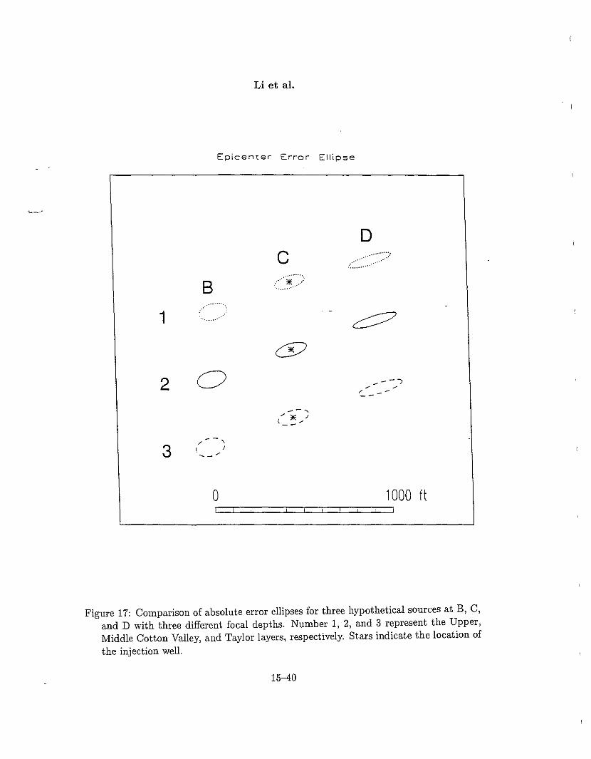
Figure 17 shows the epicenter error ellipses for three hypothetical sources (B, C, D)in three different layers (1, 2, and 3). For each of the three sources, the strike ofthe errorellipse changes little when the source depths vary. The maximum azimuth variation ofthe ellipse strike for each source at three different depths is less than 1.40

• For each of

15-13

Li et al.

Table 2: Absolute Source Location Uncertainties (0" = 10ms)

Source Strike a b dz dr dtLocation (WE) (ft) , (ft) (ft) (ft) (ms)

Al 70.8 77.8 56.8 55.3 111.1 6.17A2 71.1 80.1 57.3 55.2 112.9 6.16A3 73.8 81.3 61.8 65.1 121.1 6.20B1 71.1 81.0 45.2 46.0 103.5 6.04B2 71.2 83.6 45.5 45.0 105.2 6.02B3 72.5 83.4 50.1 57.8 113.2 6.14C1 72.2 88.7 34.3 37.9 102.4 5.72C2 72.2 91.5 34.5 36.1 104.2 5.66C3 72.7 90.5 39.0 53.1 111.9 6.01D1 75.4 126.8 25.4 31.7 133.2 5.07D2 75.4 129.9 25.6 29.5 135.7 4.96D3 75.3 131.3 29.5 50.8 143.8 5.78E1 80.0 606.7 22.3 29.7 607.8 4.76E2 80.0 619.2 22.5 27.4 620.2 4.62E3 80.0 638.1 25.9 50.0 640.6 5.67A'l 87.0 77.9 56.4 55.2 110.9 6.17A'2 86.7 80.2 56.8 55.1 112.7 6.16A'3 84.4 81.3 61.3 65.0 120.8 6.20B'l 86.8 81.1 44.8 45.9 103.4 6.04B'2 86.7 83.7 45.1 44.9 105.2 6.02B'3 85.6 83.6 49.7 57.7 113.1 6.14C'l 86.0 89.0 34.1 37.9 102.6 5.72C'2 86.0 91.8 34.3 36.1 104.4 5.66C'3 85.5 90.8 38.7 53.1 112.1 6.01D'l 83.4 128.0 25.3 31.7 124.3 5.07D'2 83.4 131.2 25.5 29.5 136.8 4.96D'3 83.4 132.6 29.4 50.8 145.0 5.79E'l 79.2 564.7 22.3 29.7 565.9 4.76E'2 79.2 576.3 22.5 27.4 577.4 4.62E'3 79.2 593.9 26.0 50.0 596.5 5.67

15-14


the three sources, the semimajor and semiminor axes of the ellipse are smallest in layer1. The semimajor and semiminor axes of the ellipse increase when the source depthsincrease. However, the maximum variation in the semimajor and semiminor axes dueto a change in source depths are less than 5 ft. Thus, we conclude that the variation oflocation uncertainties for these hypothetical sources is not significant when the sourcedepth varies from 8450 to 9750 ft.

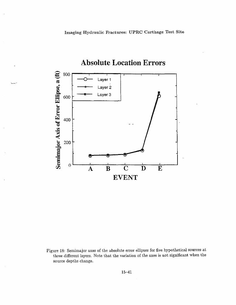
The semimajor axes, a, of the error ellipses for five hypothetical sources at threedifferent depths are plotted in Figure 18. For each of the five sources, the semimajoraxis is smallest when the sources are in the first layer (Upper Cotton Valley). If thehypothetical sources are in layers 2 and 3, the semimajor axes of the error ellipses areslightly larger than those for the sources at layer 1. But the relative variation of thesemimajor axes due to changes in the source depths is less than 5%. For hypotheticalsources A, B, C, and D, the semimajor axes of error ellipses vary from 78 to 131 ft. Thesemimajor axis of the error ellipse for hypothetical source E jumps to a range of 606to 638 ft. This is the largest value for the semimajor axis of the epicenter error ellipseand represents the maximum location error fur the epicenter if our constant (J model isreasonable.

Figure 19 shows the semiminor axes of the epicenter error ellipses for five hypothetical sources in three different layers. For each of the five hypothetical sources, thesemiminor axis is the largest when the sources are in layer 3 (Taylor). The semiminoraxes of the error ellipses for each of the five sources at layers 1 and 2 are very similar toeach other. The relative variation of the semiminor axes due to variation of the sourcedepths ranges from 9% to 16%. It is shown that the semimajor axis of the error ellipsegradually decreases, from source A to E, when the distances between the sources andthe geophone arrays decrease. The largest and smallest semimajor axes of the absoluteerror ellipses are 62 ft (at source A3) and 22 ft (at source E1).

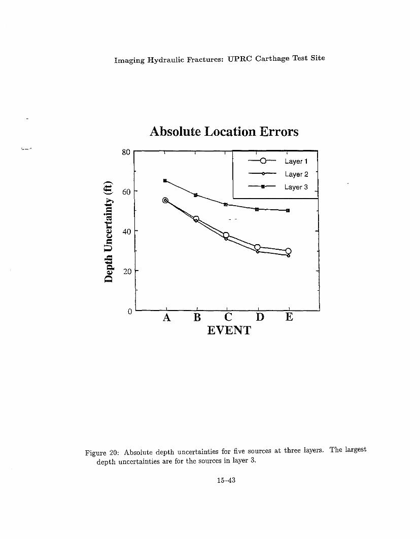
Depth uncertainties for the five hypothetical SOurces at three layers are shown inFigure 20. The depth uncertainty for each of the five sources is the largest when thesources are in layer 3 (Taylor). The major feature in the depth uncertainty plot (Figure20) is that the variation of depth uncertainties caused by changing the depths of thefive hypothetical sources is significant. The relative variation of the depth uncertaintiesdue to change of the source depths ranges from 15% (at source A) to 45% (at sourceE). It is also true that the depth uncertainties for five sources at three layers decreasewhen the distances between the sources to the geophone arrays decrease. The maximumand minimum of the absolute depth uncertainties are 65 ft (at source A3) and 27 ft (atsource E), respectively.

RELATIVE LOCATION ERRORS

Calculating the relative source location uncertainties is relatively easier than calculatingthe absolute location uncertainty because the velocity model error has been removed orat least reduced by a station correction model. Therefore, the reading error of arrival

15-15

Li et al.

times will be a major contributor to the relative source location error. It has been proventhat the waveform correlation analysis (Poupinet et aI., 1984; Ito, 1985; Fremont andMalone, 1987; Phillips et aI., 1992; Deichmann and Garcia-Fernandez, 1992; Moriyaet aI., 1994; Li et aI., 1995b, 1996) using a master-slave event pair can significantlyimprove accuracies for arrival time picks. The differential arrival times can be picked toan accuracy of one sample interval or even better (Poupinet et al., 1984; Deichmann andGarcia-Fernandez, 1992; Li et aI., 1995b). Therefore, we can approximate the readingaccuracy of the arrival times as the data variance for traveltimes in a relative sense.

In a hydrofracturing experiment in Los Alamos, the sampling rate was 5000 samplesper second (House, 1987; Phillips et al., 1992; Li et aI., 1995a, 1996). In UPRC'spilot study (Zhu et aI., 1996) and in ARCO's WDTI experiment (Atlantic RichfieldCorporation, 1994; Rieven and Rodi, 1995), 0.5 ms was used as the sampling interval.These values help us to specify the standard deviation for variances of traveltime datain a relative sense. For a conservative estimate, we selected a constant model with II =1 ms as the data variance of traveltimes for estimating relative location uncertainties.

We calculated the relative source location uncertainties with the standard deviationof II = 1 ms. The relative location uncertainties are calculated for the five hypotheticalsources (A, B, C, D, and E) and their ghost images (A', B', C', D', and E'). Theparameters describing the relative source location uncertainties include the epicentererror ellipse (strike, semimajor axis, and semiminor axis), the depth uncertainty, andthe semimajor axis of the hypocenter error ellipsoid, and the error in the estimate oforigin time. These parameters are listed in Table 3.

We compared the absolute and relative error ellipses of epicenters for three hypothetical sources (C, B, and D) at layer 2 (Middle Cotton Valley) shown in Figures 21,22, and 23. The relative error ellipses are significantly smaller than those of the absolute error ellipses by factors of 10. For the hypothetical source C2, the semimajorand semiminor axes of the error ellipse are 9.2 and 3.4 ft in the relative sense and 91.5and 34.5 ft in the absolute sense. The area of the relative error ellipse for source C2(Figure 21) is smaller than the absolute error ellipse by factors of 100. The areas of therelative error ellipses are 98.2, 106.2, 121.4 square-feet for hypothetical sources C, D,and B, respectively. The area is smallest for the source at C and then increases as thesource moves to Band D. The alb ratios of sources B, C, and Dare 1.8, 2.7, and 5.0,indicating that the error ellipse is significantly elongated from source B to D (Figures21 to 23). These numbers clearly reflect that the spatial variations are not the same forthe different location uncertainty parameters.

The different spatial variations for the semimajor and semiminor axes of the epicentererror ellipses and the depth uncertainty are further shown in Figures 24 to 26. As thehypothetical source moves from A to E, the semimajor axis (Figure 24) increases butthe semiminor axis (Figure 25) and the depth uncertainty (Figure 26) decrease. Thesemimajor axis of the relative error ellipse varies from 7.8 to 13.1 ft form source A to D,and then suddenly jumps to about 64 ft at source E. This is the largest relative locationerror for the five hypothetical sources at three different depths. The semiminor axis of

15-16


Table 3: Relative Source Location Uncertainties (0" = 1ms)

Source Strike a b dz dr dt~- .~ Location (N°E) (ft) (ft) (ft) (ft) (ms)

Al 70.8 7.8 5.7 5.5 ILl 0.62A2 71.1 8.0 5.7 5.5 11.3 0.62A3 73.8 8.1 6.2 6.5 12.1 0.62B1 7Ll 8.1 4.5 4.6 10.4 0.60B2 71.2 8.4 4.6 4.5 10.5 0.60B3 72.5 8.3 5.0 5.8 11.3 0.61C1 72.2 8.9 3.4 3.8 10.2 0.57C2 72.2 9.2 ~.4 3.6 10.4 0.57C3 72.7 9.0 3.9 5.3 11.2 0.60D1 75.4 12.7 2.5 3.2 13.3 0.51D2 75.4 13.0 2.6 3.0 13.6 0.50D3 75.3 13.1 3.0 5.1 14.4 0.58E1 80.0 60.7 2.2 3.0 60.8 0.48E2 80.0 61.9 2.2 2.7 62.0 0.46E3 80.0 63.8 2.6 5.0 64.1 0.57A'l 87.0 7.8 5.6 5.5 ILl 0.62A'2 86.7 8.0 5.7 5.5 11.3 0.62A'3 84.4 8.1 6.1 6.5 12.1 0.62B'l 86.8 8.1 4.5 4.6 10.3 0.60B'2 86.7 8.4 4.5 4.5 10.5 0.60B'3 85.6 8.4 5.0 5.8 11.3 0.61C'l 86.0 8.9 3.4 3.8 10.3 0.57C'2 86.0 9.2 3.4 3.6 10.4 0.57C'3 85.5 9.1 3.9 5.3 11.2 0.60D'l 83.4 12.8 2.5 3.2 12.4 0.51D'2 83.4 13.1 2.5 3.0 13.7 0.50D'3 83.4 13.3 2.9 5.1 14.5 0.58E'l 79.2 56.5 2.2 3.0 56.6 0.48E'2 79.2 57.6 2.2 2.7 57.7 0.46E'3 79.2 59.4 2.6 5.0 59.7 0.57

15-17

Li et al.

the relative error ellipse ranges from 2.2 ft at source E to 6.2 ft at source A. The depthuncertainty in the relative sense is smallest at source E (2.7 ft) and largest at sourceA (6.5 ft). The spatial of variation of the relative depth uncertainty is more significantthan that for the relative error ellipse of the epicenters.

We have compared the relative and absolute location uncertainties based on constanta models with absolute a = 10 ms and relative a = 1 ms. If we compare the relativelocation errors with the absolute location uncertainties estimated using the variable a

model, we still find that the relative location uncertainty parameters, such as the semimajor and semiminor axis of error ellipses and the depth uncertainty, are smaller thanthose for the absolute locations by factors of 3 to 7. The relative location uncertaintiesare significantly reduced compared to the absolute location uncertainties for both cases.

DISCUSSION

In this study, we have used two simplified velocity models and the geometry configuration of geophone arrays of the upcoming UPRC fracture experiment to obtain synthetictraveltime data and to examine the data variances of traveltimes. Using an SVD methodand the data variance models, the ahsolute and relative location uncertainties are estimated for five hypothetical sources at three different layers with depths ranging from8450 to 9750 ft. The five sources are evenly distributed along an assumed strike of anexpected fracture zone from southwest to northeast (from A to E) with spacing of 500ft. Source C is situated in the center within the fracture treatment well.

The spatial variations of the location uncertainties are clearly shown by our analyses.Both the relative depth uncertainties and the relative semiminor axes of the epicentererror ellipse decrease from source A to E. The average depth uncertainty (relative) andthe average semimajor axis (relative) for the five hypothetical sources in the three layersare 4.5 ± 1.2 ft and 3.9 ± 1.4 ft, respectively. However, the relative semimajor axes ofthe epicenter error ellipses increase from 7.8 ft at source A to 63.8 ft at source E. Thesemimajor axis of the error ellipse for source E is larger than the depth uncertainty andthe semiminor axis by factors of 13 to 25. We attribute the very large semimajor axis ofthe error ellipse for source E to the fact that it is close to the line connecting the observedarrays in the two monitor wells, MOl and M02. The ill-conditioned matrix A in equation(1) results in significantly amplifying the traveltime error to the semimajor axis of theepicenter error ellipse for source E. Therefore, one can not obtain accurate epicenterestimates for events close to source E, although the source is the closest to the twomonitor wells. The average semimajor axis of the epicenter error ellipse for source A toD is 9.6 ± 2.1 ft. In summary, our estimates of the relative source location uncertaintiesfor sources A to Dare 12 ft for the semimajor axis, 5 ft for the semiminor axis, and6 ft for the depth uncertainties. The absolute location uncertainties for correspondingsources are about 3 to 10 times larger than the relative location uncertainties.

Note that the absolute location uncertainties were conservatively estimated usingthe two simplified velocity models and should represent the upper bound of uncertainty

15-18


estimates only when the simplified velocity models approximate the real earth structure.If the real earth structure significantly differs from what we have used due to significantlateral heterogeneity, a sharp jump of velocities at interfaces, and medium anisotropy,the absolute source location uncertainties are expected to be much larger. In the caseof relative source locations, the systematic error caused by a velocity model can beremoved; the measurement accuracy for arrival times is the key factor for deriving theuncertainties of ~elative source locations. The waveform correlation analysis can achievea reading accuracy that is equal to or better than the sampling interval for unaliasingwaveform data. In our e.nalysis, we conservatively take a as 1 ms. If the a is 0.5 ms, therelative location error will be reduced by factors of 2. We strongly recommend using asampling interval of 0.5 ms or even shorter. Selecting a better sampling rate will not onlyreduce the relative location uncertainty but also avoid undersampling the seismic signals.Previous spectral analysis of microearthquakes induced by hydrofracturing (Fehler andPhillips, 1991; Li et al., 1995c) indicated that the corner frequencies of these inducedevents could be as high as 400 to 500 Hz, which is very close to the Nyquist frequencyfor a sampling interval of 1 ms. Note also that our analysis was done under an idealcase in which it is assumed that the hypothetical seismic events are recorded well byall geophones and all data can be used in estimating location uncertainties. In a realcase, it is rear that data from all the geophones can be used in locating seismic sources.Therefore, locating events without data from all geophones may result in slightly largerlocation uncertainties compared to what we have estimated.

The major purpose of the UPRC hydrofracturing experiment is to accurately imagethe hydraulic fracture and estimate its orientation, length, and height. We have derivedthe location uncertainties for the hypothetical sources along the assumed strike of theexpected fracture zone. We fOl<nd that the strike of the epicenter error ellipse is roughlyparallel to the strike of the fracture zone. Therefore, the semimajor axes of error ellipsesfor the sources situating at different parts of the fracture zone can be used to calculatethe relative measurement error for the fracture length. Between two sources C and Bin the Middle Cotton Valley, the real distance between them is 500 ft. The semimajoraxes of the absolute error ellipses for the two sources are ± 91.5 ft and ± 83.6 ft,respectively. The resulting relative measurement error for the fracture length is about35%. If the semimajor axes of the relative error ellipses are used, one can obtain therelative measurement error for the fracture length to be 4%. Figure 27 shows the relativemeasurement errors for sources distributed along the fracture zone using three differentdata variance models. The relative measurement errors are about 4% to 15% withthe relative location results, but are 25% to 150% when the absolute location resultsare used. Although the error is smaller for source A, the longest distances betweenthe source and two monitor wells may cause a poor signal-to-noise ratio, especially forsmaller events, resulting in poor location results. Similarly, we can estimate the relativemeasurement error of the fracture height.

In this study, we theoretically predict the absolute and relative location uncertainties for the given velocity models, the geometry of the fracture and monitor wells, and

15-19

Li et al.

the geophone array configuration in the monitor wells. The analysis of the location uncertainties provides some ideas about how accurately the fracture azimuth, length, andheight can be estimated in locating microearthquakes induced by hydraulic fracturing.We have found that relative source locations can significantly reduce relative measurement error for fracture length, azimuth, and height. We have also realized significantspatial variations of the absolute and relative location uncertainties. These results leadus to believe that our location uncertainty analysis should be generalized as a practicaltool for optimally designing a two-well seismic monitoring system to accurately imagesubsurface hydraulic fractures. For the given velocity models, the geometry of the fracture, and the geophone array configuration in the monitor wells, we can search for theoptimal positions for two monitor wells so that the location uncertainties (especiallythe depth uncertainty or one of the error ellipse axes) of sources along the fracture areminimized. Alternatively, for the given velocity models, the geometry of the fracture,and the positions of two monitor wells, one can determine how many geophones in amonitor well are necessary to achieve required location accuracies. Accomplishing thisapproach successfully will significantly contribute to_ accurate, efficient, and economicimaging of subsurface fractures.

CONCLUSIONS

We have theoretically predicted the relative and absolute location uncertainties (95%confidence regions) for hypothetical sources at three different depths along an assumedstrike of a target fracture zone with given velocity models, the configuration of 96three-component geophones in the boreholes, and the locations of two monitor wells.The assumed strike of the expected fracture zone was N70°E. The five hypotheticalsources are evenly distributed along the fracture zone and span a distance range of 2000ft with spacing of 500 ft. The vertical extent of the hypothetical sources ranges from8450 to 9750 ft. We determined that the typical relative location uncertainties for thefive hypothetical sources at three different layers are 12 ft for the semimajor axis, 5 ftfor the semiminor axis, and 6 ft for depth uncertainty. It is shown that the relativelocation uncertainties are significantly smaller than those of the absolute location byfactors of 3 to 10. The relative measurement error for the fracture length is about 4%to 15% when the relative source location results are used. The location ambiguity fromthe two-station locations is discussed and the arrival azimuth data are recommendedfor removing such location ambiguity. We expect that our approach of the locationuncertainty analysis can be generalized as a practical tool in optimally designing of atwo-well seismic monitor system for high-precision imaging of subsurface fractures.

15-20


ACKNOWLEDGMENTS

We would like to thank Dr. Roger Turpening for helpful discussions. This researchwas supported by the Reservoir Delineation Consortium at ERL and by DOE Contract#DE-FG02-86ERI3636.

15-21

Li et al.

REFERENCES

Atlantic Richfield Corporation, 1994. The deep well treatment and injection program,fracture technology filed demonstrate project, Final Report, The Atlantic RichfieldCorporation, Plano, Texas, 84 pp.

Block, L.V., C.H. Cheng, M.C. Fehler, and W.S. Phillips, 1993. Seismic imaging usingmicroearthquakes induced by hydraulic fracturing, Geophysics, 59, 102-112.

Bratt, S.R., and T.C. Bache, 1988. Locating events with a sparse network of regionalarrays, Bull. Seism. Soc. Am., 78, 780-798.

Castagna, J.P., 1993. Petrophysical imaging using AVO, The Leading Edge, 12, 172-178.Deichmann, N. and M. Garcia-Fernandez, 1992. Rupture geometry form high-precise

relative hypocenter locations of microearthquake clusters, Geophys. J. Int., 110,501-517.

Douglas, A., 1967. Joint epicenter determination, Nature, 215, 47-48.Fehler, M., L. House and H. Kaieda, 1987, Determining planes along which earthquakes

occur: method and application to earthquakes ac-cempanying hydraulic fracturing,J. Geophys. Res., 92, 9407-9414.

Fehler, M. and W.S. Phillips, 1991. Simultaneous inversion for Q and source parametersof microearthquakes accompanying hydraulic fracturing in granitic rock, Bull. Seism.Soc. Am., 81, 553-575.

Fremont, M.J. and S.D. Malone, 1987. High precision relative locations of earthquakesat Mount St. Helens, Washington, J. Geophys. Res., 92, 10223-1023.

House, L., 1987. Locating microearthquakes induced by hydraulic fracturing in crystalline rock, Geophys. Res. Lett., 14, 919-921.

Ito, A., 1985. High resolution relative hypocenters of similar earthquakes by crossspectral analysis method, J. Phys. Earth, 33, 279-294.

Jordan, T.H., and K.A. Sverdrup, 1981. Teleseismic location techniques and their application to earthquake clusters in south-central Pacific, Bull. Seism. Soc. Am., 71,1105-1130.

Kijko, A., 1977. An algorithm for the optimum distribution of a regional seismic network,Pure Appl. Geophys. 115, 999-1021.

Lawson, C.L., and R.J., Hanson, 1974. Solving Least Squares Problems, Prentice Hall,Inc. 340 pp.

Lee, W.H.K., and S.W. Stewart, 1981. Principles and applications of microearthquakenetworks, Adv. Geophys. Suppl. 2, 293 pp.

Li, Y. and C.H. Thurber, 1991. Hypocenter constraint with regional seismic data: a theoretical analysis for the Natural Resources Defense Council Network in Kazakhstan,USSR, J. Geophys. Res., 96, 10159-10176.

Li, Y., C.H. Cheng, and M.N. Toksiiz, 1995a. Hydraulic fracture imaging from the LosAlamos hot dry rock experiment, Proceedings of SEG International Explosion and65th Annual Meeting, Huston, Texas, 223-226.

Li, Y., C. Doll, and M.N. Toksiiz, 1995b. Source characterization and fault plane deter-

15-22


minations for Mblg = 1.2 to 4.4 earthquakes in the Charlevoix seismic zone, Quebec,Canada, Bull. Seism. Soc. Am., 85, 1604-1621.

Li, Y., C.H. Cheng, and M.N. Toksoz, 1995c. Source characterization of microearthquakesinduced by hydraulic fracturing with empirical Green's function, Annual Report,Borehole Acoustics and Logging and Reservoir Delineation Consortia, MIT, Cambridge, Massachusetts, 7.1-7.26.

Li, Y., C.H. Cheng, and M.N. Toksoz, 1996. Seismic imaging geometry and growthprocess of a hydraulic fracture zone at Fenton Hill, New Mexico, Submitted to Geophysics.

Magotra, N., N. Ahmed, and E. Chael, 1981. Seismic event detection and source locationusing single station (three-component) data, Bull. Seism. Soc. Am., 77, 958-971.

Moriya, H., K., Nagano, and H. Niitsuma, 1994. Precise source location of AE doubletsby spectral matrix analysis of triaxial hodogram, Geophysics, 59, 36-45.

Phillips, W. S., L. S. House, and M. C. Fehler, 1992. VpjVs and the structure of microearthquake clusters, Seismol. Res. Lett., 63, 56-57.

Poupinet, G., W. L., Ellsworth, and J. Frechat,- 1984. Monitoring velocity variations inthe crust using earthquake doublets: An application to the Calaversa fault, California, J. Geophys. Res., 89, 5719-5731.

Rieven, S. and W. Rodi, 1995. Analysis of microseismic location accuracy for hydraulicfracturing at the DWTI site, Jasper, Texas, Annual Report, Borehole Acoustics andLogging and Reservoir Delineation Consortia, MIT, Cambridge, Massachusetts, 5.17.28.

Rodi, W., Y. Li, and C.H. Cheng, 1993. Location of microearthquakes induced byhydraulic fracturing, Annual Report, Borehole Acoustics and Logging Consortium,MIT, Cambridge, Massachusetts, 369-410.

Thurber, C.H., H. Given, and J. Berger, 1989. Regional seismic event location with asparse network: Application to eastern Kazakhstan, USSR, J. Geophys. Res., 94,17767-17780.

Truby, L. S., RG., Keck, and R.J. Withers, 1994. Data gathering for a comprehensivefield fracturing diagnostics project: A case study. SPE/IADC Paper 27516, presentedat the SPEjIADC Drilling Conference, Dallas, Texas, February 18-20.

Uhrhammer, R A., 1980. Analysis of small seismographic station network, Bull. Seism.Soc. Am., 70, 1369-1379.

Vinegar, H., P. Wills, D. DeMartini, J., Shlyapobersky, W. Deeg, R Adair, J. Woerpel,J. Fix, and G. Sorrells, 1992. Active and passive imaging of a hydraulic fracture indiatomite, J. Petrol. Tech., 44, 28-34, 88-90.

Wills, P.B., D.C., DeMartini, H.J., Vinegar, J., Shlyapobersky, W.F., Deeg, J.C., Woerpel, J.E., Fix, G.G., Sorrells, and RG., Adair, 1992. Active and passive imagingof hydraulic fractures, The Leading Edge, 11, 15-22.

Zhu, X., J. Gibson, N. Ravindran, R Zinno, D. Sixta, 1996. Seismic imaging of hydraulicfractures in Carthage tight sands: A pilot study, The Leading Edge, 15, 218-224.

15-23

Li et al.

#22-9Monitor Well

Figure 1: Schematic of a proposed UPRC hydraulic fracturing experiment in the CarthageField, Panola County, Texas.

15-24

,-


UPRC: Hydrofracture Experimentft

3000 f- 0 Frac. Well ' I ££ Monitor Well MOl

...- ...... Fracture

2500 ..

2000 -e···..······..·..........··......·..

......·......·..........·....·..·~Ol£

M021500 l- N -

+ E

1000, ,

1000 1500 2000 2500 3000 ft

Figure 2: Plane view of the planned experiment area in Carthage Field showing thelocations of a treatment well and two monitoring wells. The dashed line indicatesan assumed azimuth of an expected hydraulic fracture.

15-25

Li et al.

UPRC-Project: Sensor Distribution7500

• ••• •• •• •• •• •• •• •• •• •• "• •• "• •• 1: Upper Cotton Valley

•• •

8500 • •• •• •• •

--- • •c:: • •

• •- • •• 2: Middle Cotton Valley

•.c • •

• •.... • •Cl. • •~ • •

• •Q • "• "• •

• •9500 • •

• •• •• •• 3: Taylor •• •• "• •• •• •• ••••

MOl M02#22-9 #21-9

10500

Figure 3: Cross-section of two monitor wells (M01=#22-9, M02=#21-9) at CarthageField indicating the locations of seismometers and lithological units.

15-26


86

10

Velocity12

(kft/s)14 16 18

8

--~..::d'-"

10..c......Q.Q,)

Q12

14

,,\..

"",

\

\",\

\,\

\,

\\ Vs,

Vp

Figure 4: Linear gradient velocity models for P- and S-waves for the experimental siteat Carthage Field,

15-27

Li et al.

Hypothetical seismic sources along frature

ft

5000 .6. Monitor Well N

0 Frac. Well + E-e- Seismic Source

4000

3000

MOl

.6.

2000

DE

.6.M02

1000

5000 ft4000300020001000O'----'--...J--'---'---------.J.----'--.J---..-......l...--l

o

Figure 5: Map view showing the locations of one treatment well (open circle) and twomonitor wells (triangles) and five hypothetical seismic sources (solid circles labeledwith A, B, C, D, and E) along an expected strike of a hydraulic fracture zone.

15-28


Location ambiguity with two arrays

ft

5000

4000

A Monitor Well N

0 Frac. Well +-e-- Real EventE

····0..· Imaginary Event

D

3000

2000

1000

FOI

MOl.

AE

.....{).......···{)..·_··..o.._ ..oE' D' C' B' A'

AM02

1000 2000 3000 4000 5000 ft

Figure 6: Map view showing the location ambiguity of five hypothetical seismic sourcesalong the strike of an expected hydraulic fracture zone. Open circles connected witha dashed line represent ghost images of five hypothetical sources.

15-29

Li et al.

Monitor Well: MOl

8

---<:::~'-'.: 9....Cl.<I,l

Q

10

..............~'-'~"

...~..................•

..............~'"

......................

..................

p

s

Source @ Cl

4-4 -2 0 2

D-Time(ms)Monitor Well: M02

11 '--~----'_~-..L_~-.J..._~-'-_~--I

-6

8

---<:::~'-'.c 9....Cl.<I,l

Q

10

................

.•.•...•.•..........•..•..•..

................

p.__.... s

...............................

Source @ Cl

42-4 -2 0

D-Time(ms)Figure 7: Traveltime differences between a linear gradient and a constant velocity model

for a hypothetical seismic source (Cl) at the Upper Cotton Valley to the two seismicarrays in the monitor wells.

15-30


Monitor Well: MOl

8

---ot:..:.::'-'.c 9-C.

QJ

Q

10

...............

p

...._ ..... S

.•.•.•.•.•...•...•...•.........

........•.•...•.......•...•

...•.....•...•.•.•....

Source @ A3

11-4 -2 0 2 4 6 8 10

D-Time(ms)

Monitor Well: M027

p

.............. S

8•.•.•.•.•...•.•......

---ot:..:.:: ........'-'.. 9 '.".-- ",c. '.....

QJ '.................Q

10......

Source @ A311

-4 -2 0 2 4 6 8 10

D-Time(ms)Figure 8: Traveltime differences between a linear gradient and a constant velocity model

for a hypothetical seismic source in the layer of Taylor (A3) to the two seismic arrays.

15-31

Li et al.

Travel Time Data Variation

-0-- L1-MAX

II L2-MAX

• L3-MAX

··_····0···_· L1-RMSI< di ... .......-)(...... L2-RMS

··_····tIt····· L3-RMS

di ZHU-96

20

---~_ .. tile'-'- 15C':l='t:l••til~

~~e 10••--~;;..C':llo<

E-i~ 5;;..C':l

~rJJ

0A B c D E

HYPOTHETICAL EVENT

Figure 9: Comparison of the maximum and RMS (dashed lines) S-wave traveltimeresiduals for five sources at three different layers. The solid line with triangles is theerror in traveltimes derived by Zhu et al. (1996).

15-32


Location ArnDiguity and Epicenter Error Ellipse

Constont Sigmo = 10 ms

[:, M01

Ao

Bo

CCV

F01

o

E --

"'~[:, M02

....,' .

C' B'

2000 It

A'

Figure 10: Absolute epicenter error ellipses, estimated with the constant II model, forfive hypothetical seismic sources at layer 2 along the assumed strike of the hydraulicfracturing zone and their ghost images. Note that the semimajor axes of error ellipsesfor sources E and E' are extremely large.

15-33

Li et al.

Location ArTlbiguity and Epicenter Error Ellipse

Variable Sigma = 3.5 to 6.5 ms

Ao

/.:::, M01

ED ..: •... -:::

C ~

B = E' D' C'11/

0 F01 /.:::,M02

o

....'.....

B' A'

2000 It

Figure 11: Absolute epicenter error ellipses, estimated with the variable (7 model, forfive hypothetical seismic sources at layer 2 along the assumed strike of the hydraulicfracturing zone and their ghost images. Note the difference in the error ellipsescalculated with two different (7 models.

15-34


Constant vs. Variable Sigma Model~_ .. 80

-0- Constant Sigma

--- • Variable Sigma0::'-'

a 60

=.-eo:....~Q,lu 40=0-=....Q.Q,l

20Q

o~-A-'----==B----::C::----':D~--;E-:::-----'

EVENT

Figure 12: Absolute depth uncertainties estimated for five sources at layer 2 with twodifferent (J models.

15-35

Li et al.

Constant vs. Variable Sigma Model,-.~ 80 r---r---r---,--....,..-,....----,...-----,'-'

60 ~_-:- .-J

--0-- Constant Sigma

• Variable Sigma

o~-A-'----LB-~C:c-------JD--E.l-------l

EVENT

20

Figure 13: Absolute semiminor axes of error ellipses derived for five sources at layer 2with two different (J models.

15-36


Constant vs. Variable Sigma Model---¢:: 700'-'~ --0- Consiant SigmatI.lQ. 600 • Variable Sigma0---~'"' 500Q

'"''"'~ 400....Q~

e':l300~

tI.l0:;<~ 200

'"'Qo~

e':l 100eOs~ 0rr.J A B C D E

EVENT

Figure 14: Absolute semimajor axes of error ellipses calculated for five sources at layer2 with two different (J models.

15-37

Li et al.

10

Constant Sigma

Variable SigmaII

o'-----A:-----:;B~--:C~---::!D~--:!E!:-----l

EVENT

20

Constant vs. Variable Sigma Model

~ 30

Figure 15: The ratio of absolute semimajor and semiminor axes of error ellipses are the

same.

15-38


Constant Vs. Variable Sigma Model,.Q 5~~

-0-~ Constant Sigma~rr.>Q.. 4 • Variable Sigma.-- ----~<t:·~C •·~ 3·::~O"

rr.>·0~o=0 2~o~.-I.-Q..l><i~'-'

..... Ic~~•-< 0

A B C D E

EVENT

Figure 16: Comparison of the areas of the absolute error ellipses estimated with twodifferent (J models. Note that the area of source D at layer 2 calculated with thevariable (J model is the smallest.

15-39

o

Li et al.

Epicenter Error Ellipse

DC

............... ..

B )I(...........

1 ~

@

2 0 -- - .....//

/--,)I( /

( -- -3

".- - '\

I I---1000 It

c:::::r::===:::::r==r:::::c::::r::=::~

Figure 17: Comparison of absolute error ellipses for three hypothetical sources at B, C,and D with three different focal depths. Number 1, 2, and 3 represent the Upper,Middle Cotton Valley, and Taylor layers, respectively. Stars indicate the location ofthe injection well.

15-40


Absolute Location Errors

--- 800it::'-' ~ Layer 1ce~

Q,l • Layer 2"lCl. • Layer 3.-- 600-r.:lr....er....

r.:l 400~Q

"l.-il<-<

r.... 200Q.~ceS.-SQ,l 0IJJ A B C D E

EVENT

Figure 18: Semimajor axes of the absolute error ellipses for five hypothetical sources atthree different layers. Note that the variation of the axes is not significant when thesource depths change.

15-41

Li et al.

Absolute Location Errors,-..<::= 70'-' --0- Layer 1,.Q~

60 • Layer 2Q,lfI.IQ. • Layer 3---- 50~-e 40-~....c 30fI.I--~-< 20-c=-S 10--S

Q,l 0rJl A B C D E

EVENT

Figure 19: Semiminor axes of the absolute error ellipses for five hypothetical sources atthree different layers. Note that the axes are largest for sources at layer 3 (Taylor).

15-42


Absolute Location Errors80 r--,----,---r1---r--"r---,

,.-,

~ 60

~=.-~

1::~ 40

=~

;5" 20Q

••

•

Layer 1

Layer 2

Layer 3

•

o'---A:----:B:!::--C~--=D---=!::E-.-J

EVENT

Figure 20: Absolute depth uncertainties for five sources at three layers. The largestdepth uncertainties are for the sources in layer 3.

15-43

Li et at.

::::C'icenter C::rr~'" Ellipse: ~e!ative vs. A,bsolute

oC2

o 100 it

Figure 21: Relative (solid line) and absolute (dashed line) epicenter error ellipses forsource C2.

15-44


t:::;:;icen'ter Error ~',I-,pse-_ ~ I -_ -::e alive vs. .~bsc!ute

C82

o 100 ft

Figure 22: Relative (solid line) and absolute (dashed line) epicenter error ellipses for

source B2.

15-45

Li et al.

E:Jicenter- ~r;,"8r E.:ipse: .::::elative ".'s. ,4.bsolute

~

D2

o 100 ft

Figure 23: Relative (solid line) and absolute (dashed line) epicenter error ellipses forsource D2.

15-46


Relative Location Errors,-.,it: 80'-' -0-C': Layer 1~

~ • Layer 2enC. •.- 60

Layer 3--~l-oe""~ 40....cen.~

<"" 20c.~

C':S.-S~ 0r.n A B C D E

EVENT

Figure 24: Semimajor axes of the relative error ellipses for five hypothetical sources at

three different layers.

15-47

Li et al.

Relative Location Errors,-,¢; 10'-',.Q -0- Layer 1~

ClJ 0 Layer 2tilc.. 8... • Layer 3--~l.<

e 6l.<~....0til 4.~

-<l.<0 2=·s·S

ClJ 07J:J A B C D E

EVENT

Figure 25: Semiminor axes of the relative error ellipses for five hypothetical sources atthree different layers. Note that the axes are largest for sources at layer 3 (Taylor).

15-48


Relative Location Errors:.._..

7-0- Layer 1

0 Layer 2..-- 6c= • Layer 3'-'

~

=.- sC':lt::~Col

=P 4.c-Q"~

Q 3

2 L...---:-A-~:--:::--~-...J..----lBCD E

EVENT

Figure 26: Relative depth uncertainties for five sources at three layers. The largestdepth uncertainties are for the sources in the layer 3. Note the spatial variation of

the relative depth uncertainties.

15-49

Li et al.

Fracture Length Estimates

--- 160=-_0- ~ • ABSOLUTE: Constant Sigma

'-' 140r..Q .. ABSOLUTE: Variable Sigmar..r.. 120~ -0- RELATIVE: Constant Sigma....= 100~e~ 80r..=~ 60~~ 40;;..........ell 20-~~

°A B C DB C D E

Figure 27: Relative measurement error for estimating the fracture length calculated withthree different (]" models. The smallest relative measurement error for the fracturelength are obtained with the relative location results.

15-50

imaging hydraulic fractures: source location …

Documents