`Imaging System for theMeasurement of Body and Head

Motion and Gaze Visualization fora Video-Based Eye Tracker`

Constantin Rothkopf

Advisor: Dr. Jeff Pelz

• A very brief review of eye movements

• The main idea: measuring head movements

• The device:

– mechanical setup

– calibration

– data acquisition

– data processing

• Application of the device: Classification of eye

movements

• Results

Overview

Design of the human image detector

• The human image detector has a highly anisotropic

design: high visual acuity is only available in a small central region of the retina, the fovea

Stare at the ‘x’ Do not move your eyes !

• The solution to the acuity problem: eye movements

– the eyes are moved to 'point to' objects or regions in the

scene that require high acuity

– eye movements are also made toward task-relevant targets

even when high spatial resolution is not required

• Humans typically carry out more than 100,000 eyemovements a day, which reach velocities of up to 600

degrees per second

Eye movements

Types of eye movements

Fixations Saccades Smooth pursuits VORs

head still, head could be moving, head still, head moving,

eyes fixating eyes moving to new target eyes following target eyes pointing on target

Eye tracker

Dual Purkinje Tracker

Limbus Tracker

The RIT-Wearable-Eye-Tracker 1

color CMOS scene camera

calibration LASER

hot mirror

folding mirror

IR illuminator/optics module

monochrome CMOS eye camera

The RIT-Wearable-Eye-Tracker 2

Video based eye tracker

• An infrared diode illuminates the

eye

• The retina reflects the infrared

light very well

• The eye camera of the eye

tracker records the position of

the pupil together with the

specular reflection

• Using image processing the

position of the eye is calculated

• Understanding human perception:

– Where and when do humans focus visual attention?

– How does the brain process visual information?

– How is the visual scene represented in the brain?

• Biologically inspired data processing:

– Robot vision

– Avatar vision, Animat vision

• Engineering applications:

– Gaze position dependent information display

– ‘Smart media’ systems, augmented reality

• Marketing

Impact of eye movement research

change blindness example by Jason Babcock

• Most of the classification is carried out by trainedexperts who compare the captured video sequences

from the eye camera and the scene camera of theeye tracker

• During the last 30 years a number of algorithmic

approaches for the classification have beendeveloped

• These algorithms were developed under the

assumption that the head is fixed

• No algorithms were developed for the classification ofsmooth pursuits and VORs

Eye movement classification

The idea

• In natural tasks the subject interacts purposefully witha changing environment: How do we use vision?

• A lightweight video-based eye tracker allows the

subject to move their head and body in an almostnatural way

• By measuring the head movements it is possible to:

– distinguish smooth pursuits and VORs

– measure the gaze direction relative to the environment

– study head and eye coordination

• Is it possible to extract the head motion form the imagesequence from the scene camera of the eye tracker?

• Three commonly used methods for ego-motion estimation:

– epipolar geometry

– optical flow

– global estimation oftransformation

(automated image

registration)

• The global estimationmethod was implemented

using an image sequencefrom the scene camera

Ego-motion estimation 1

• The problem: rotation and translation can result in ambiguous

patterns because the point of expansion may be locatedoutside of the field of view

• Low accuracy

Ego-motion estimation 2

translation rotation

• Spherical projection of environment reduce ambiguity of image

transformation under translation and rotation significantly

• Both the point of expansion and the point of contraction arevisible on the sphere

Ego-motion estimation 3

translation rotation

Omnidirectional vision sensors

• Baker and Nayar (1999) have shown that an

omnidirectional vision sensor with a single viewpointcan be constructed using a hyperbolic mirror and a

perspective camera or with a parabolic mirror and anorthographic camera

• If the systems has a single viewpoint, it is possible to

map the captured omnidirectional image to a planarperspective image

• System used for this project:

– hyperbolic mirror from Accowle Ltd., a=8.37mm, b=12.25mm,

rtop=26mm

– standard NTSC miniature video camera with 360 lines

resolution

Mechanical setup of the device

ASL 501 eye tracker ISCAN eye tracker

Camera calibration

• The camera was calibrated usingthe Matlab calibration toolbox

• Pinhole-camera model:

q: pixel coordinates, u: normalized image coordinates

• Camera model including radial andtangential distortion:

Kuq =

˙˙˙

˚

˘

ÍÍÍ

Î

È

˙˙˙

˚

˘

ÍÍÍ

Î

È

⋅

⋅

=

1100

qkf0

q0kf

z

y

zx

v0v

u0u

• Hyperbolic mirror:

• Intersection between ray fromworld point X through focal point

and mirror:

• Tracing ray back from image pixel

q to the mirror:

with K, the camera calibration

matrix and tc=2e

Geometry of catadioptric system

2b2aeb

yx

a

)(z 1,2

22

2

2

+=++

=-e

c

1-1

h )f( tqKqKX +⋅=-

2

2

22

1

22

3

2

3

2

vavavb

)a(evb)f(

--

+=

vv

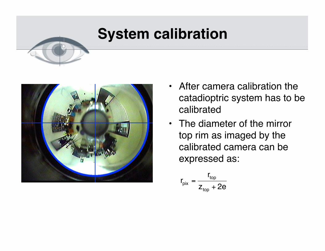
• After camera calibration thecatadioptric system has to be

calibrated

• The diameter of the mirrortop rim as imaged by the

calibrated camera can beexpressed as:

System calibration

2ez

rr

top

top

pix+

=

Remapping the image

Image captured by catadioptric system remapped to q,f space, 512x512

• Three approaches:

– Epipolar geometry (Svoboda,Pajdla,Hlavac 1998)

– Optical flow (Gluckman, Nayar 1998)

– Spherical harmonics (Makadia & Daniilidis 2003)

• When using epipolar geometry a feature tracker is needed totrack corresponding points between images

• Optical flow methods have been used with higher resolution

cameras and are reported to be very susceptible to noise,including occlusion

• The method using spherical harmonics decomposition has

been shown to work well because of its global character

Rotation estimation 1

• Spherical harmonics basis-functions on the sphere:

• with the Associated LegendreFunctions:

• and the Legendre polynomials:

• The spherical harmonics buildan orthonormal set of basis

functions on the sphere

Rotation estimation 2

Real part of spherical harmonics:

vertically: 0 £ l £ 4

horizontally: -l £ m £ +l

ö

∂èöè

imm

lm)!(l4

m)!1)(l(2lm

l )e(cosP),(Y+

-+=

(x)P)x(11)((x)P ldx

d2mm

l m

m2m

--=

[ ]l2

l

l

ll 1)(xdx

d

l!2

1(x)P -=

Rotation estimation 3

• The discrete spherical harmonics coefficients:

• A rotation of a function on the sphere can

be parameterized with ZYZ Euler angles:

• Under this rotation the new coefficients can be expressed as:

where the Plmn are generalized associated Legendre functions

 Â-

=

-

=

⋅⋅=12B

0j

12B

0i

ij

m

lijjB∂ ),ö(èY),öf(èam)(l,f

)

áãâáâã

iml

pm

ipl

pm

l

lp

l

pmlplm e))(cos(Pe)),,(g(U with (g),Uff --+

-=

⋅⋅=⋅= Â))

)()R()R(R),,g( zyz áâããâá =

Rotation estimation 4

• The common trick: the rotation can be reparametrized as:

• The advantage is that the unknown variables appear only in the

exponents:

• The problem to solve is then:

),,(,0)g,(g),,g(222221∂∂∂∂ ã∂âáãâá +++=

)),ã∂,(â(gU,0)),(á(gUff2∂

2∂

2

l

lp

lkm

l

lk2∂

2∂

1lpklplm ++⋅+= Â Â

+

-= -=

))

lp

∂)ik(â-l

lp

l

km

l

lk

l

pklp

)ip(á)im(ã

lm f(0)eP(0)Pfeef 2∂

2∂ +

+

-= -=

+-+-

  ⋅⋅=)

0)(tf)(tf(0)e(0)PP)(tfee

2l

0m

2lp

l

lp

l

lk

1lp

∂)ik(âl

km

l

pk1lp

)ip(á)im(ãl

1p

2∂

2∂

=˙˚

˘ÍÎ

È-⋅⋅⋅Â Â ÂÂ

= -= -=

+-+-+-

=

• This equation can be minimized using Quasi-Newton Methodslike Broyden’s Method

• Newton’s Method:

with xn+1: next iterate, xn: previous iterate, F’(x): the Jacobian

of the function F(x)

• Broyden’s method uses a different update rule:

• The Matlab library implementing Broyden’s method by

C.T.Kelley was used

Rotation estimation 5

)F(x)(xFxx n

1

nn1n

-

+¢-=

)F(x)F(x)x(xBwith),F(xBëxx 1nn1nnnn

1

nnn1n --

-

+ -=--=

• Three Matlab functions:

– image sequence is remapped onto the unit sphere and

stored

– spherical harmonic coefficient are calculated from

remapped image sequence and stored in a text file

– rotation estimation from stored spherical harmonics

coefficients

• The processing time is reduced by precalculatingthe mapping transformation and the spherical

harmonics

Implementation of rotation estimation

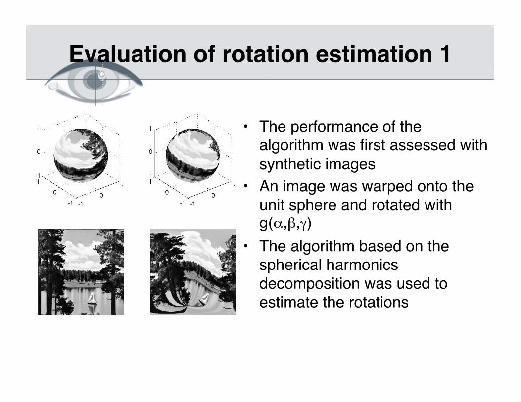
Evaluation of rotation estimation 1

• The performance of thealgorithm was first assessed with

synthetic images

• An image was warped onto theunit sphere and rotated withg(a,b,g)

• The algorithm based on thespherical harmonics

decomposition was used toestimate the rotations

Image size: 1024x1024:

angle l£5 l£8 l£12

a=10º 9.87º 9.91º 9.61º

b =10º 10.08º 10.12º 10.53º

g =10º 9.92º 9.77º 9.93º

Image size: 512x512:

angle l£5 l£8 l£12

g =5º xxº xxº xxº

g =10º xxº xxº xxº

g =25º 25.15º xxº xxº

g =65º 64.47º xxº xxº

Evaluation of rotation estimation 2

Combining the data

• Several algorithms described in the literature based on threeideas:

– eye movement velocity criterion (thresholding)

– spatial clustering (for fixed head position)

– statistical modeling (Hidden Markov Model)

• Most algorithms were developed assuming fixed head positionsfor use in tasks like reading, equation solving, signal detection,

and image quality evaluation

• No algorithms have been developed for the classifications ofeye movements including fixations, saccades, smooth pursuits,

and VORs

Classification of eye movement types

• Discrete time: t, t+1, t+2, …

• State sequence: Q = { qt , qt+1 , qt+2 , … }

• Observation sequence: O = { Ot , Ot+1 , Ot+2 , … }

• Transition probabilities: aij = P( qt+1= Sj | qt =Si )

• Probabilities of observation variable: Pj( Ot ) ~ Normal( mj , sj2 )

Hidden Markov Model 1

Distribution in S1 Distribution in S2

Hidden Markov Model 2

• Salvucci (1999) used a 2-stateHMM for the classification of

fixations and saccades

• The observation variable is theeye-in-head velocity

• The distributions of thesevelocities are modeled withGaussian distributions

• The parameters of the transitionprobabilities aij and the

parameters of the velocitydistribution mj, sj are estimated

from the data with the Baum-

Welsh algorithmVelocity distribution

for fixation (deg/sec)

Velocity distribution

for saccade (deg/sec)

Hidden Markov Model 3

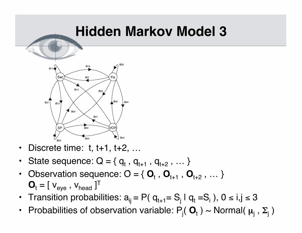
• Discrete time: t, t+1, t+2, …

• State sequence: Q = { qt , qt+1 , qt+2 , … }

• Observation sequence: O = { Ot , Ot+1 , Ot+2 , … }Ot = [ veye , vhead ]

T

• Transition probabilities: aij = P( qt+1= Sj | qt =Si ), 0 £ i,j £ 3

• Probabilities of observation variable: Pj( Ot ) ~ Normal( mj , Sj )

Preliminary classification results

• A total of 3 minutes of smooth pursuits of variousvelocities and VORs were recorded from one

subject

• The head movements were measured using a

magnetic Fastrack system

• The algorithm was able to classify the occurringfixations, saccades with 100% accuracy

• 65% of the smooth pursuits and 100% of the

VORs were classified correctly

Work to do...

• Validation of classification results throughcomparison with expert classification

• Develop a system with a higher resolution camera

for better accuracy

• Implementing the nonlinear minimization in C

… a special thank you

...for a great undergraduate experience at the Centerfor Imaging Science

to Dr. Jeff Pelz for the introduction to research in visual

perception

to Dr. Elliott Horch for being a model advisor and greatteacher

to Dr.Roger Easton for the introduction to the joy oflinear systems

to Dr. Jon Arney for reminding me

to Jason Babcock for the

Questions!