imf country report no. 14/69 canada · stress testing—technical note ... stress test matrix ......
TRANSCRIPT

© 2014 International Monetary Fund
IMF Country Report No. 14/69
CANADA FINANCIAL SECTOR ASSESSMENT PROGRAM STRESS TESTING—TECHNICAL NOTE This Technical Note on Stress Testing on Canada was prepared by a staff team of the International Monetary Fund as background documentation for the periodic consultation with the member country. It is based on the information available at the time it was completed in February 2014. The policy of publication of staff reports and other documents by the IMF allows for the deletion of market-sensitive information.
Copies of this report are available to the public from
International Monetary Fund Publication Services
700 19th Street, N.W. Washington, D.C. 20431 Telephone: (202) 623-7430 Telefax: (202) 623-7201
E-mail: [email protected] Internet: http://www.imf.org
Price: $18.00 a copy
International Monetary Fund Washington, D.C.
March 2014

CANADA FINANCIAL SECTOR ASSESSMENT PROGRAM
TECHNICAL NOTE ON STRESS TESTING
Prepared By Monetary and Capital Markets Department
This Technical Note was prepared by IMF staff in the context of the Financial Sector Assessment Program in Canada. It contains technical analysis and detailed information underpinning the FSAP’s findings and recommendations.
February 2014

CANADA
2 INTERNATIONAL MONETARY FUND
CONTENTS Glossary ___________________________________________________________________________________________ 4
INTRODUCTION AND OVERVIEW _______________________________________________________________ 5
A. Overview of Stress Tests _________________________________________________________________________ 5
SCENARIOS ______________________________________________________________________________________ 10
BANKING SECTOR—SOLVENCY STRESS TESTS _______________________________________________ 12
A. Bottom-up Stress Test _________________________________________________________________________ 14
B. IMF Top-down Stress Test _____________________________________________________________________ 23
C. OSFI Top-down Stress Test ____________________________________________________________________ 36
D. Reconciliation of Results ______________________________________________________________________ 39
E. Recommendations and Policy Implications ____________________________________________________ 42
BANKING SECTOR—LIQUIDITY AND FUNDING STRESS TESTS—INDIVIDUAL AND NETWORK
EFFECTS _________________________________________________________________________________________ 43
A. Recommendations and Policy Implications ___________________________________________________ 54
LIFE INSURANCE SECTOR—SOLVENCY STRESS TEST _________________________________________ 55
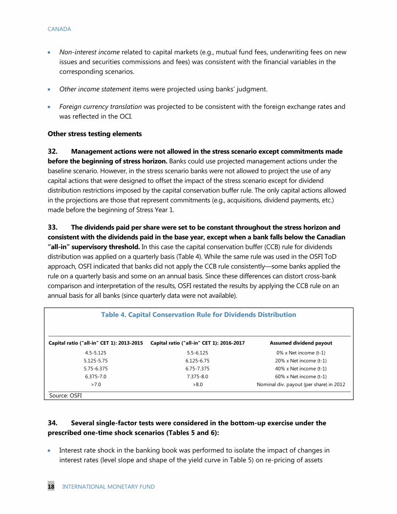
CMHC SOLVENCY STRESS TEST ________________________________________________________________ 58
References _____________________________________________________________________________________ 100 TABLES 1. Stress Testing Recommendations _______________________________________________________________ 9 2. Regulatory and Supervisory Capital Requirements ____________________________________________ 14 3. Mapping Economic Sectors from the BU into Economic Sectors Used in BoC Estimation of PDs ____________________________________________________________________________________________ 16 4. Capital Conservation Rule for Dividends Distribution _________________________________________ 18 5. IRBBB Spreads Under the Stress-test Scenario ________________________________________________ 19 6. Trading Book Risk Parameters Under the Stress-test Scenario ________________________________ 20 7. Mapping Basel II Asset Classes and Exposures by Economic Sectors into New Basel II Asset Classes ___________________________________________________________________________________________ 26 8. Dividends Distribution Schedule_______________________________________________________________ 31 9. Main Differences Between Different Approaches ______________________________________________ 41 10. FSIs: Big 6 versus the Rest of the Banking System ____________________________________________ 61 11. Summary of Banks’ Stress Testing Results ___________________________________________________ 68 12. Liquid and Illiquid Assets of the BSL Metric—Haircuts Calibration ___________________________ 84 13. Outflows of BSL Metric—Run-off Rates Calibration __________________________________________ 85

CANADA
INTERNATIONAL MONETARY FUND 3
14. Stress Test Matrix (STeM): Solvency and Liquidity Risks and Network Effects ________________ 86
FIGURES 1. IMF Top Down Approach ______________________________________________________________________ 23 2. Geographical and Sectoral Distribution of Losses and Exposures _____________________________ 32 3. IMF TD Solvency Stress Test Results—Sensitivity Analysis _____________________________________ 35 4. Macro-financial Risk Assessment Framework (MFRAF) of the BoC ____________________________ 44 5. MFRAF Modules _______________________________________________________________________________ 45 6. MFRAF Modulus Timing _______________________________________________________________________ 46 7. The BoC Liquidity and Network Stress Test Results, Baseline Scenario ________________________ 50 8. Aggregate Loss Distributions, Baseline Scenario ______________________________________________ 51 9. The BoC Liquidity and Network Stress Test Results, Adverse Scenario ________________________ 53 10. Aggregate Loss Distributions, Adverse Scenario _____________________________________________ 53 11. Total MCCSR Ratio in Baseline and Adverse Scenario ________________________________________ 56 12. Total Tier 1 Ratio in Baseline and Adverse Scenario __________________________________________ 56 13. Net Income in Baseline and Adverse Scenario _______________________________________________ 57 14. Contribution to MCCSR Deviation from Baseline _____________________________________________ 58 15. Developments in Banking Sector _____________________________________________________________ 62 16. Scenarios—Canada, Main Variables __________________________________________________________ 69 17. Scenarios—US, Euro Area, Other, Main Variables ____________________________________________ 70 18. IMF Top Down Model of Income Statement—Interest Income ______________________________ 71 19. IMF Top Down Model of Income Statement—Interest Expense ______________________________ 72 20. IMF Top Down Model of Income Statement—Trading Income ______________________________ 73 21. IMF Top Down Model of Income Statement—Non-interest Income _________________________ 74 22. IMF Top Down Model of Income Statement—Non-interest Expense ________________________ 74 23. IMF Top Down Assumptions—Loans, Deposits ______________________________________________ 75 24. IMF Top Down Assumptions—Loans, Balance Sheet _________________________________________ 76 25. Solvency Stress Test Results __________________________________________________________________ 77 26. Drivers of Stress Test Results—Contributions to CET1 Change _______________________________ 78 27. Drivers of Stress Test Results—Contributions to Net Income ________________________________ 79 28. Net Income and RWAs—Comparison ________________________________________________________ 80 29. Net Income and RWAs—Comparison ________________________________________________________ 81 30. Parameters of RWAs and Expected Losses—Comparison ____________________________________ 82 31. Recapitalization Needs—as Percent in gross income ________________________________________ 83
BOX 1. OSFI Algorithm to Project Loan Book _________________________________________________________ 38
ANNEX I. Statistical Annex ________________________________________________________________________________ 61
CANADA
4 INTERNATIONAL MONETARY FUND
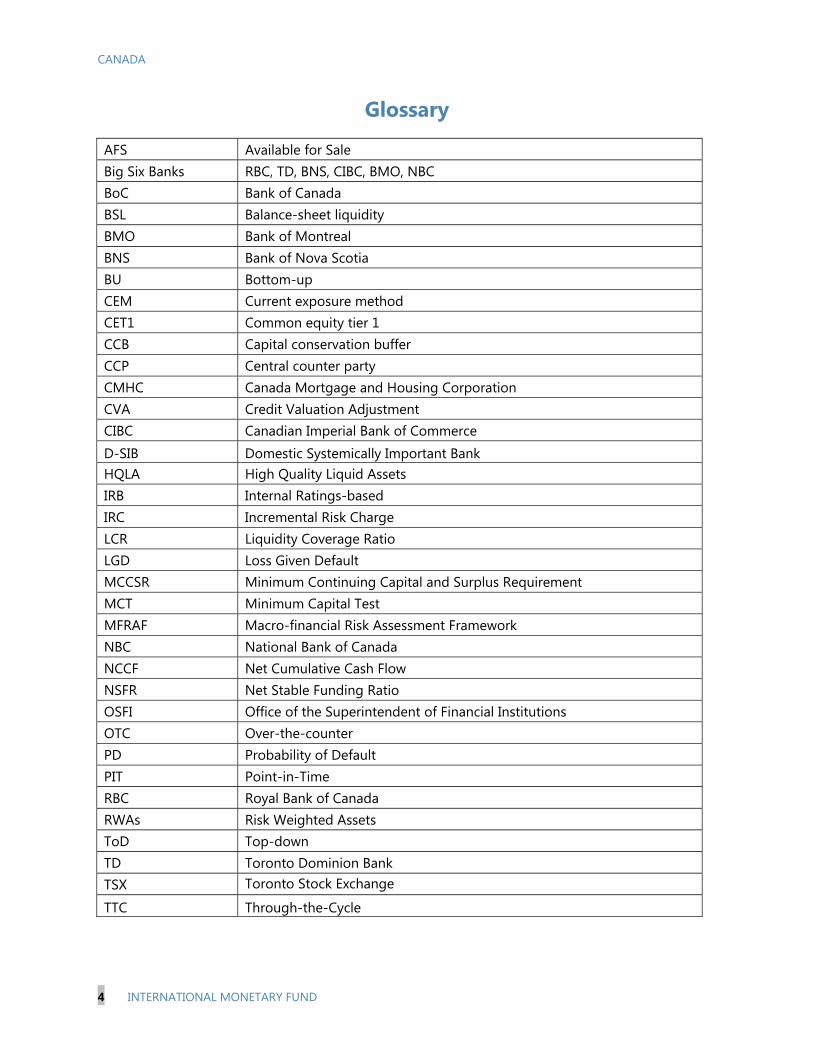
Glossary
AFS Available for Sale Big Six Banks RBC, TD, BNS, CIBC, BMO, NBC BoC Bank of Canada BSL Balance-sheet liquidity BMO Bank of Montreal BNS Bank of Nova Scotia BU Bottom-up CEM Current exposure method CET1 Common equity tier 1 CCB Capital conservation buffer CCP Central counter party CMHC Canada Mortgage and Housing Corporation CVA Credit Valuation Adjustment CIBC Canadian Imperial Bank of Commerce D-SIB Domestic Systemically Important Bank HQLA High Quality Liquid Assets IRB Internal Ratings-based IRC Incremental Risk Charge LCR Liquidity Coverage Ratio LGD Loss Given Default MCCSR Minimum Continuing Capital and Surplus Requirement MCT Minimum Capital Test MFRAF Macro-financial Risk Assessment Framework NBC National Bank of Canada NCCF Net Cumulative Cash Flow NSFR Net Stable Funding Ratio OSFI Office of the Superintendent of Financial Institutions OTC Over-the-counter PD Probability of Default PIT Point-in-Time RBC Royal Bank of Canada RWAs Risk Weighted Assets ToD Top-down TD Toronto Dominion Bank TSX Toronto Stock Exchange
TTC Through-the-Cycle

CANADA
INTERNATIONAL MONETARY FUND 5
INTRODUCTION AND OVERVIEW1 A. Overview of Stress Tests
1. This technical note reports on the stress testing module of the 2013 FSAP Update for Canada. It describes the coverage of the exercise; tail risks relevant to the Canadian financial system and its major institutions and their quantification; assumptions and models used to measure the impact of tail event realization on the financial system. An important objective of the exercise was to assist the FSAP in identifying risk factors that are more likely to weigh on financial results during a period of severe stress. The note includes recommendations for the Canadian authorities, derived from this joint exercise, to enhance the individual components of their stress testing framework.
2. Coverage was broad. Stress tests covered three major segments of the domestic financial sector and most of its systemically important financial institutions. Within the banking industry, this included the six largest Canadian banks that together constitute over 90 percent of the banking system by assets. The three largest life insurance providers, with over 60 percent market share in terms of premiums, were part of the exercise as was the Canada Mortgage and Housing Corporation (CMHC), a crown corporation and the largest mortgage insurer with a 70 percent market share, also in terms of premiums.
3. The exercise was comprehensive in terms of the types of stress tests applied, the number of risk factors against which financial institutions’ resilience was tested, and the range of sensitivity analyses against which the robustness of the results reported was checked. Stress tests applied: Banks were subjected to both bottom-up (BU) and top-down (ToD) stress
tests. There were three ToD models used, developed by the Bank of Canada (BoC), the IMF, and the Office of the Superintendent of Financial Institutions (OSFI). Life insurance companies and CMHC participated in the BU exercise.
Range of risk factors tested against: Banks’ resilience was tested against credit, market, and operational risks impacting earnings and solvency in a tail risk scenario under the BU test. Under the ToD tests credit and market risks were assessed. In addition, the BoC’s ToD model was utilized to assess the additional impact on bank solvency of second-round stress arising out of idiosyncratic, contagion-driven, funding runs and asset fire-sales as well as counterparty credit losses associated with interbank exposures.
1 Prepared by Timo Broszeit, Ivo Krznar and Jay Surti (MCM). The FSAP team would like to express its deep gratitude to counterparts at Office of Superintendent of Financial Institutions and Bank of Canada for close collaboration in facilitating this comprehensive stress testing exercise; and to the stress testing teams at the banks (RBC, TD, BNS, BMO, CIBC, NBC) and insurance companies (Manulife, Sunlife, Great WestCo) and CMHC, which participated in the bottom-up solvency stress testing exercises.

CANADA
6 INTERNATIONAL MONETARY FUND
Sensitivity analyses performed: Alternative approaches to stress testing banks in this FSAP provided a useful assessment of the robustness of results to alternative parameterizations of the risk model. A good example of this was the calculation of key risk-sensitive components of earnings and solvency metrics in the credit risk analysis; e.g., regulatory versus economic approaches to deriving risk-weighted assets under stress in the BU and OSFI ToD modules versus the IMF ToD module.
4. Common set of assumptions and input parameters. Notwithstanding differences in calculation of risk-sensitive components of the earnings and solvency metrics, the assumptions behind the stress and baseline scenarios and input risk parameters, including probabilities of default and loss-given defaults2, that were utilized under the alternative approaches were identical, to enhance comparability of the results obtained. BU analyses conducted by the life insurance companies and by CMHC assessed the earnings and solvency implications of the same set of shocks as applied to banks under the tail risk scenario. All banking sector tests were conducted on a consolidated basis data as of October 2012 which were, for solvency stress tests, restated to reflect early full adoption of Basel III. The stress tests for life insurers and CMHC were conducted based on end-2012 valuations.
5. Scenarios. The stress tests considered two scenarios over a five year horizon - a baseline and a stress scenario. The baseline scenario reflects the IMF‘s World Economic Outlook projections as of February 2013. The stress scenario is the result of a model-driven simulation of a shock of a severe crisis beginning outside Canada, which has a severe impact on the Canadian financial system and economy, notably as it triggers the materialization of a key domestic risk (household finances and housing prices). This simulation results in a hypothetical scenario represented by a full set of variables (“shocks”) that are then translated into stress testing results. The simulation exercise brings about a cumulative decline in real GDP over a three-year period (on an annual basis) which represents the most severe recession in the last 35 years.3 After three years of recession, the GDP growth rate gradually returns to positive levels. This severe scenario translates into elevated probabilities of default. For life insurers, the stress scenario affects the balance sheet mainly via lower asset values within the investment portfolio-interest rates, credit spreads, equity prices and currency movements.
6. Bank solvency stress tests suggest that, while all banks would fall below the Canadian “all-in4” CET1 supervisory threshold during severe economic distress, the resulting recapitalization needs are manageable. Solvency stress tests assessed the level of banks’ “all-in” 2 In comparison to probabilities of default, which were prescribed by the authorities, loss given defaults were the result of bank’s internal projections. 3 Canada has not seen a negative GDP growth rate in two consecutive years, since 1981. This is probably true for even a longer time span but data limitations prohibit comparisons with recessions prior 1981. 4 “All-in” is defined as capital calculated to include all of the Basel III regulatory adjustments that will be required by 2019 (i.e., no phase-ins) but retaining the Basel III phase-out rules for non-qualifying capital instruments.

CANADA
INTERNATIONAL MONETARY FUND 7
Common Equity Tier 1 ratios against the regulatory threshold consistent with the Basel III transition schedule and the Canadian “all-in” supervisory threshold of 7 percent for the first three years, and 8 percent for the last two years. The Basel III framework was introduced by OSFI in January 2013 and included early adoption of Basel III supervisory adjustments. The three tests used the same confidential supervisory data, including parameters of expected losses and the IRB formula for risk-weighted assets (RWAs).
Notwithstanding quantitative differences, all tests suggest that most banks “all-in” CET1 ratios will fall below the Canadian “all-in” CET1 supervisory threshold by 2015 with recapitalization needs peaking in 2016, under the IMF approach, at 30 percent of 2012 gross income or 150 percent of 2012 net income (corresponding to 2½ percent of 2015 nominal GDP). This is expected given banks’ capital position in the base year relative to the Canadian “all-in” CET1 supervisory threshold, which incorporates early adoption of both the Basel III thresholds and supervisory adjustments. Moreover, four banks would fall below the regulatory minimum for the first time in 2016 under the IMF approach, mainly due to introduction of the D-SIB surcharge, with recapitalization needs five times smaller (½ percent of 2015 nominal GDP) than capital needed to bring all banks to supervisory threshold.
Looking at the peak of the system-wide “all-in” CET1 ratio (in the base year) to its trough across the different approaches, the IMF ToD model appears most conservative—the system-wide “all-in” CET 1 ratio would fall by 2½ percentage points in 2015 relative to the base year or 5½ percentage points relative to the baseline scenario in 2015.
While the drivers of capital positions are similar, quantitative effects differ across the various approaches. This is partly explained by different modeling choices of the mapping between the macroeconomic shocks and banks’ capital positions. Effects on capital ratios in the period of negative economic growth are largely driven by RWAs for credit risk in the IMF ToD, and credit losses in all three approaches mostly due to the recession’s impact on default rates and NPLs. Losses are concentrated in Canada and the U.S. Around 65 percent of losses at their peak (2015) come from Canadian exposures (mostly consumer loans, construction, and manufacturing) and around 25 percent from U.S. exposures (mostly business loans). Assumptions governing dividend payouts also has an important effect on capitalization in OSFI’s top-down and bottom-up exercise.
7. Bank liquidity stress tests suggest that, in aggregate, banks could withstand severe funding and market liquidity shocks as characterized by withdrawal of funds and haircuts on liquid assets similar to emerging liquidity standards. However, most banks would face substantially greater solvency pressures when subjected to additional increases in parameters related to asset fire-sale discounts and roll-over rates.
BoC MFRAF. The MFRAF presents a novel approach to assessing the solvency impact of funding liquidity and contagion pressures (the liquidity module) and spillover effects (the network module) that may arise as second-round effects within the stressed macroeconomic environment. In the IMF stress tests in past FSAPs, funding liquidity impact was approximated by higher funding costs. This is
CANADA
8 INTERNATIONAL MONETARY FUND
the first time that a framework has been used that models interactions between credit and liquidity risk in a financial system where banks are linked through interbank exposures. In the baseline liquidity scenario, the results of the liquidity module suggest that liquidity risk would result in a limited additional impact on banks’ CET1 ratio, thus suggesting that in aggregate, banks would be able to endure such liquidity stress conditions. However, one bank is affected significantly by funding liquidity risk: this is due to the combination of the impact of credit losses on its capital position before the liquidity risk materialized, and a mismatch in maturing liabilities and assets that can be sold in the distressed period. In the adverse liquidity scenario, the marginal impact of liquidity risk brings four banks’ “all-in” CET1 below 4.5 percent.
Spillover effects between the six largest banks appear limited. The marginal impact of the network effect on “all-in” CET1 is rather small and ranges between 21 and 29 basis points. This is because interbank exposures are brought down significantly by collateralization and hedging. In general, banks maintain small exposures in the interbank market, keeping spillover risk quite low. Even the exposures to other Canadian financial institutions (mostly pension funds and life insurance companies) and non-Canadian bank counterparties in the interbank (mostly U.S. banks) are small. Therefore, any contagion effects arising outside of the major Canadian banks would be limited.
8. The three large life insurance companies show quite robust results in the stress test. In the baseline scenario the companies increase their capital ratio, based on the MCCSR, from an aggregated 2012 value of 215 percent to 288 percent at the end of the projection horizon in 2017; while in the adverse scenario, solvency ratios of all companies remain well above the supervisory target of 150 percent, based on the MCCSR. On aggregate, total MCCSR ratios decline from 215 percent in 2012 to 199 percent in 2015, stabilizing thereafter. Net income remains positive under the adverse scenario in each year of the projection horizon and is expected to recover quickly from its lows in 2013. On aggregate, net income declines by 20 percent in 2013 and rises in each year thereafter. Share price declines and adverse policyholders’ lapse rates add most to the overall impact on insurers’ capital and net income under the adverse scenario.
9. Bottom up stress tests implemented by the Canada Mortgage and Housing Corporation assesses the value of claims under the stress scenario to be much larger than under the baseline scenario, and this lowers the solvency ratio significantly. The capital adequacy based on the Minimum Capital Test (MCT) drops sharply but remains above the minimum regulatory level of 100 percent. However, various management actions could be taken in times of severe stress, e.g., new business could be re-priced and underwriting could be concentrated in lower risk loans. Net income turns significantly negative in 2013, but recovers quickly and is positive again in 2016 and 2017.
10. While the authorities’ stress testing framework is well advanced, the exercise has suggested that there is room for improvement (Table 1).

CANADA
INTERNATIONAL MONETARY FUND 9
Table 1. Stress Testing Recommendations
OSFI
Banking stress test
Complement OSFI top-down stress testing framework for banks with economic (risk-sensitive) concepts of key credit risk input parameters (and review assumptions regarding the dividend distribution) and econometric, model-based approaches based on longer time series of balance sheet and income statement data. Para 38, 40, 41, 46, 48, 62
Start collecting longer time series including more granular data (e.g., trading income). Para 46, 62
Ensure consistent implementation of some of the key elements of the BU stress testing exercise across different banks. Para 62
Enhance the liquidity stress testing framework by running tests based on the LCR and NSFR on a regular basis Para 77
Insurance stress test
Provide a comprehensive set of assumptions which can be applied by participating companies in a harmonized manner; expand analytical approaches used to verify stress test results against supervisory data. Para 85, 86
BoC
Find a meaningful way of calibrating liquidity losses. Para 67, 77
Model the Balance Sheet Liquidity ratio in an internally consistent manner. Para 77
Embed MFRAF in a macroeconomic model (DSGE or econometric). Para 77
General
Include major regulated entities at federal and provincial level in a regular, common stress testing exercise, which would involve a degree of collaboration between relevant federal and provincial authorities. Para 62
11. The rest of the Technical Note explains in detail the solvency and liquidity stress tests that were conducted in the context of the 2013 Canada FSAP. After reviewing the main assumptions of the two scenarios, the next section presents three different approaches of the FSAP’s solvency stress test of the banking sector, analyzes the results of the tests and reconciles the findings of different test results. For comparability purposes, the explanation of each approach is structured in the same way, providing details of the main determinants of solvency risk—credit losses, risk weighted assets, income statement items (excluding charge for impairment) and other stress testing elements—that have an impact on the capital position of banks. The findings of the liquidity stress testing exercise are presented in the third
CANADA
10 INTERNATIONAL MONETARY FUND
section together with more elaborate discussion of the BoC macro-financial risk assessment framework which models funding liquidity risk and spillover effects as endogenous outcomes of credit risk, market liquidity risk and the liquidity profile of the banks. The liquidity section is followed by a stress-test analysis of the life insurance sector and of the largest mortgage insurer.
SCENARIOS 12. Two macroeconomic scenarios, over five-year horizons, were consistently applied in the BU and IMF ToD stress testing approaches.5 The paths under the stress scenario of other relevant macroeconomic and financial variables were generated by the central bank using its own macroeconomic models. The proposed scenarios and corresponding paths of macroeconomic variables that reflect point-in-time risks are:
A baseline scenario consistent with the IMF country desk projections for the stress tests horizon that follows the February 2013 World Economic Outlook update.
An adverse scenario generated using the BoC’s (DSGE) models of the domestic and global economies and staff judgment, capable of incorporating the combined impact of simultaneous movement in all the risk factors elaborated in the risk assessment matrix as part of a tail risk scenario. The simulation of the model is a hypothetical stress scenario characterized by a U-shaped recession caused by a significant deterioration of the euro area crisis. A cumulative decline in real GDP over a three-year period (on an annual basis) represents the most severe recession over a long period of time.
Baseline scenario
13. In the baseline scenario, GDP was expected to gain new momentum due to the strengthening of the U.S. economy starting mid-2013. However, the negative carry-over from a weak second half of 2012 meant that the average rate of growth for 2013 was expected to be a modest 1.7 percent.
14. After 2013, annual growth in output was expected to accelerate to slightly below 2½ percent, a pace consistent with a gradual absorption of the output gap and a corresponding convergence of unemployment to its natural rate (estimated at about 6¾ percent).
15. The forecast was based on a smooth rotation over the medium term of the main drivers of growth, away from private consumption and residential investment and toward net exports and business investment. It was expected that domestic imbalances related to household debt and the housing market will unwind gradually and that domestic demand will return to a more sustainable pace of growth while the slack in the external sector is gradually reabsorbed as the United States closes its output gap. In particular:
5 OSFI stress testing analysis included only the adverse scenario.

CANADA
INTERNATIONAL MONETARY FUND 11
As external conditions gradually improve, activity will receive a boost from net exports.
Business investment was expected to be a key driver of domestic demand, with consumption remaining subdued as household leverage stabilizes.
Fiscal policy was expected to continue to hamper growth, although less so than in 2012, while monetary policy remained highly accommodative.
Stress scenario
16. The tail risk scenario begins with a disorderly default in a peripheral euro area country, impairing other European sovereigns’ access to debt markets, resulting in turn, in a severe and persistent economic recession within the context of a deepening banking crisis in the euro zone. These problems lead to a general retrenchment from risk in the global financial system with significant adverse effects on the prices of a wide range of risky assets and higher costs for banks, including U.S. and Canadian banks. Simultaneously, risk premia rise everywhere, including the U.K., the U.S. and Canadian markets. This adverse dynamic triggers, through confidence and wealth channels, a discrete drop in global growth, including in emerging markets, putting significant downward pressure on global demand for commodities and resulting in a marked decline in commodity prices.
17. In the United States, risk premium and wealth effects lead to a severe tightening of lending standards and a marked deterioration in business investment and consumption. Economic fragility is heightened by the fiscal constraint required from the positive resolution of the fiscal cliff by the U.S. government with the aim of improving the sovereign debt situation. Overall, this leads to a protracted recession which lasts 6 quarters, accompanied by a persistent increase in the unemployment rate (with a peak at 12.4 percent in 2016Q2-Q3).
18. Under this scenario, Canada faces financial headwinds, a large foreign demand shock, decreasing commodities prices, rising uncertainty and adverse confidence and wealth effects affecting both businesses and households. Besides the corresponding sharp decline in domestic demand, Canadian banks face rising funding costs and pressure on asset quality which results in significantly tighter lending standards. In this context, Canadian households reduce their consumption and residential expenditure. Overall, the Canadian economy experiences 9 quarters of negative growth and recovers gradually over the last two and a half years of the 5-year stress horizon. National house prices decline by 34 percent over the first 3 years of the stress scenario horizon, with prices in Toronto and Vancouver declining by an additional 20 percent (54 percent in total). The unemployment rate rises steadily to peak at 13.2 percent in the beginning of the fourth year before decreasing very gradually afterwards. In this extremely unfavorable context, Canadian households seek to improve their balance sheets (deleveraging), and significantly reduce their demand for credit. At the same time, demand for business credit is also lethargic given the unfavorable economic environment and heightened uncertainty.

CANADA
12 INTERNATIONAL MONETARY FUND
BANKING SECTOR—SOLVENCY STRESS TESTS 19. In general, the capital position of a bank depends on net income after dividend payout and on RWAs. Bank capital is affected by net income where the charge for impaired credit is usually the main loss driver. For RWAs, the regulatory definition would entail an increase under the stress scenario reflecting mainly changes in credit quality, whereas the economic definition would also take into account the interaction between credit quality parameters (i.e., between Probabilities of Default—PDs—and Losses Given Default—LGDs) and the higher (positive) correlation in asset quality during times of stress.
20. A three-pronged approach was used for solvency stress testing:
The IMF ToD solvency test: The IMF test follows the balance sheet-based approach similar to Schmieder et al. (2011). This assesses the solvency of individual banks under the macroeconomic scenarios described, through changes in net income and RWAs. This approach resembles the BU stress test. However, in contrast to banks’ analysis, we try to base our framework on “economic” measures of solvency, both capital and RWAs.
The OSFI ToD solvency test: OSFI’s approach follows a template similar to the BU and IMF approaches. Income statement items, including the charge for impairment, were calculated based on corresponding balance sheet items which were projected using loan dynamics prescribed in the stress scenario. The charge for impairment is projected using a calibrated law of motion for loan loss reserves, consistent with the balance sheet projections. RWAs for credit risk were calculated using risk weights from the previous year’s BU stress scenario applied to exposures consistent with the stress scenario.
Bottom up test: the six largest banks used their internal models to stress-test the income statement, balance sheet, RWAs and some parameters of expected losses (e.g., LGDs) and RWAs (credit quality migration only, PD and LGDs were not stressed for credit risk against the tail risk and baseline scenarios). All projections and assumptions should have been consistent with assumptions specified in the scenarios and instructions provided by OSFI and the BoC. The charge for impairment reflects, in addition to the impact of the assumed increase in allowances for identified impairment,6 projected changes in the collective allowance for unidentified impairment. No capital actions that were designed to offset the impact of the stress scenario on the bank, other than dividend distribution restrictions imposed by the capital conservation buffer rule, were allowed. Market risk RWAs were stressed by setting the VaR to Stressed VaR when GDP growth rate is negative and incremental risk charge was calculated based on stressed correlations.
6 These should have been the greater of (i) banks’ own projected credit losses, and (ii) the expected credit losses defined as the product of the stressed PDs provided by the BoC, stressed LGDs projected by banks, and exposures.

CANADA
INTERNATIONAL MONETARY FUND 13
Several single-factor tests also were considered in the bottom-up exercise: (i) interest rate shock in the banking book to isolate the impact of re-pricing of assets, liabilities and off-balance sheet positions, (ii) market risk shock in the trading book, AFS securities and CVA to isolate the impact of market risk shocks on the trading book, AFS securities and on CVA on the OTC derivatives, and (iii) incremental risk charge RWAs. All these tests used one-time shock scenarios which are somewhat more severe than the environment in the first year of the stress scenario.
21. All stress tests used supervisory consolidated data of individual firms. The stress tests covered six major commercial banks, which account for about 90 percent of the banking sector’s assets. The data came from regulatory returns and files which were sent to banks by OSFI as part of the stress testing exercise.
22. Losses on banks’ insured mortgage portfolios were not analyzed in the banks’ solvency stress tests because they represent contingent liabilities of the Federal government. While the expected losses on insured mortgage portfolios were calculated in the banks’ stress test, the LGD parameter reflected the government’s guarantee - making these losses very small. However, a comprehensive analysis of losses on insured mortgages in the stress scenario was part of the CMHC stress test.
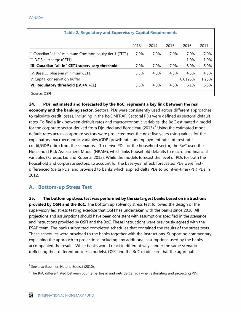
23. The capital definition applied in the stress tests corresponds to that required by local regulation i.e., OSFI’s “all-in” Basel III CET1 application. The cut-off date of the data was the fourth quarter of fiscal year 2012 (i.e., the end of October 2012). Since Basel III regulations were implemented in January 2013, the data on capital and RWAs were restated by the banks to reflect the Basel III calculation. By using restated values, the problem of estimating the impact of transition from Basel II to Basel III on RWAs and capital was circumvented. In order to assess the potential impact of negative shocks on the capital requirement metrics over the five-year risk horizon, solvency stress tests were conducted against hurdle rates consistent with both the Basel III transition schedule (the “regulatory threshold”) and local supervisory requirements (Canadian “all-in” CET1 supervisory threshold) taking into account that the Canadian authorities have chosen an accelerated implementation of Basel III threshold levels (Table 2). “All-in” capital ratios were calculated to include all of the Basel III regulatory adjustments that will be required by 2019. The common equity surcharge associated with D-SIB status that will be introduced in January 1, 2016 was also taken into account.
CANADA
14 INTERNATIONAL MONETARY FUND
2013 2014 2015 2016 2017
I. Canadian "all-in" minimum Common equity tier 1 (CET1) 7.0% 7.0% 7.0% 7.0% 7.0%II. DSIB surcharge (CET1) 1.0% 1.0%III. Canadian “all-in” CET1 supervisory threshold 7.0% 7.0% 7.0% 8.0% 8.0%
IV. Basel III phase-in minimum CET1 3.5% 4.0% 4.5% 4.5% 4.5%V. Capital conservation buffer 0.6125% 1.25%VI. Regulatory threshold (IV.+V.+II.) 3.5% 4.0% 4.5% 6.1% 6.8%
Table 2. Regulatory and Supervisory Capital Requirements
Source: OSFI
24. PDs, estimated and forecasted by the BoC, represent a key link between the real economy and the banking sector. Sectoral PDs were consistently used across different approaches to calculate credit losses, including in the BoC MFRAF. Sectoral PDs were defined as sectoral default rates. To find a link between default rates and macroeconomic variables, the BoC estimated a model for the corporate sector derived from Djoudad and Bordeleau (2013).7 Using the estimated model, default rates across corporate sectors were projected over the next five years using values for the explanatory macroeconomic variables (GDP growth rate, unemployment rate, interest rate, credit/GDP ratio) from the scenarios.8 To derive PDs for the household sector, the BoC used the Household Risk Assessment Model (HRAM), which links household defaults to macro and financial variables (Faruqui, Liu and Roberts, 2012). While the models forecast the level of PDs for both the household and corporate sectors, to account for the base-year effect, forecasted PDs were first-differenced (delta PDs) and provided to banks which applied delta PDs to point-in-time (PIT) PDs in 2012.
A. Bottom-up Stress Test
25. The bottom up stress test was performed by the six largest banks based on instructions provided by OSFI and the BoC. The bottom up solvency stress test followed the design of the supervisory led stress testing exercise that OSFI has undertaken with the banks since 2010. All projections and assumptions should have been consistent with assumptions specified in the scenarios and instructions provided by OSFI and the BoC. These instructions were previously agreed with the FSAP team. The banks submitted completed schedules that contained the results of the stress tests. These schedules were provided to the banks together with the instructions. Supporting commentary, explaining the approach to projections including any additional assumptions used by the banks, accompanied the results. While banks would react in different ways under the same scenario (reflecting their different business models), OSFI and the BoC made sure that the aggregates
7 See also Gauthier, He and Souissi (2010). 8 The BoC differentiated between counterparties in and outside Canada when estimating and projecting PDs.
CANADA
INTERNATIONAL MONETARY FUND 15
obtained from the banks’ projections are consistent with the aggregates provided in the scenarios. While taking into account the prescribed credit growth, the banks used their internal models to stress-test their incomes, balance sheets, RWAs and some parameters of expected losses against the tail risk and baseline scenarios over the five year horizon. In addition to undertaking the scenario-driven stress test, banks were asked to perform a number of singe-factor tests against different prescribed scenarios.
Credit losses
26. Credit losses were calculated as an increase in allowances for identified and unidentified impaired credit by economic sectors. The charge for impairment that enters the income statement was set equal to the assumed increase in allowances for identified losses and banks’ assumptions about the collective allowance for unidentified impairment. The assumed increase in allowance for identified losses (individual allowances and collectively-assessed allowances for individually-insignificant impaired assets) was calculated as the greater of banks’ projected losses and the expected losses.9 While projected losses result from banks’ internal models, expected losses were calculated as a product of PIT PDs, stressed LGDs and exposures at default (standardized and IRB) by economic sectors (Table 3).10 Banks were instructed to apply the BoC forecast of the delta PIT PDs by economic sectors to their own estimate of PIT PDs in the base year.11 The stressed LGDs came from banks’ internal models and were consistent with the scenarios.
9 The impact of changes in individual allowances on net exposures treated under the Standardized approach was reflected in revised risk-weighted assets. 10 Insured mortgage loans were classified as other Canadian exposure. To calculate expected losses on insured mortgages banks applied either a PD of the government or a PD of uninsured mortgage loan and an LGD which reflected the government guarantee and was thus very small. 11 These estimates were based on banks’ historical experience using weighted default rates of non-defaulted exposures.

CANADA
16 INTERNATIONAL MONETARY FUND
Banks' economic sectors BoC economic sectors
Financial institutions Financial institutionsCanadian governments Canadian governmentsAgriculture AgricultureFishing and trappingLogging and forestryMining, quarrying and oil wellsManufacturingMultiproduct conglomeratesOther business loansConstruction / real estate ConstructionTransportation, communication and other utilities Accommodations
Non-residential Mortgages Accommodations
Service AccommodationsWholesale trade Wholesale tradeRetail Small busines loansConsumer loans Consumer loansResidential mortgages (uninsured) Residential mortgagesHELOCs (uninsured)
Manufacturing
Economic sectors for which PDs were estimated
CanadaAccommodationsAgricultureConstructionManufacturingWholesaleCanadian governmentsFinancial institutionsSmall business loansResidential mortgages (uninsured)HELOCs (uninsured)Consumer loansOtherUSBusiness loansGovernmentsCommercial real estateResidential mortgages (uninsured)HELOCs (uninsured)Consumer credit card loansOther consumer loansOtherEurope (same change in PDs for all sectors)Business loansGovernmentsResidential mortgages (uninsured)Consumer loansOtherLatin America and Carribean (same change in PDs for all sectors)Business loansGovernmentsResidential mortgages (uninsured)Consumer loansOtherRest of the world (same change in PDs for all sectors)Business loansGovernmentsResidential mortgages (uninsured)Consumer loansOther
Table 3. Mapping Economic Sectors from the BU into Economic Sectors Used in BoC Estimation of PDs
Source: BoC
RWAs
27. RWAs for credit risk were affected by changes in Through-the-Cycle (TTC) PDs and changes in the credit quality of banks’ exposures. TTC PDs were updated for the new PIT PDs. Credit quality was projected by banks to be consistent with the scenarios. For Internal Ratings Based (IRB) exposures, performing credits were redistributed among borrower rating buckets and among different IRB buckets based on banks’ internal models or judgment where borrowers were expected to move under the two scenarios. For “standardized” exposures, a migration of agency ratings for some exposures was done. TTC PDs and downturn LGDs were not recalibrated. Moreover, performing credits were migrated to default status at rates consistent with the scenarios. The coverage of exposures included drawn and undrawn commitments. Exposures denominated in

CANADA
INTERNATIONAL MONETARY FUND 17
foreign currencies or measured using Mark-to-Market pricing conventions (e.g., derivatives) were recalculated to reflect the scenarios’ variables.
28. Full implementation of the credit valuation adjustment (CVA) charge was assumed to take effect from 2012 even though implementation has been delayed for regulatory capital reporting. RWAs for counterparty credit risk and CVA were calculated based on Basel III rules. Banks treated all central clearing counterparties (CCPs) as qualified CCPs unless they had reason to believe otherwise. The Current Exposure Method (CEM) was used for calculating credit counterparty risk RWAs, and the Standardized CVA capital charge with CEM-based exposure at default being used to calculate CVA capital requirements. The mark-to-market component of CEM-based exposures was changed according to the scenarios.
29. The calculation of Market Risk RWAs was affected by assumptions on the VaR and the incremental risk charge (IRC) in the stress scenario. During a period of negative GDP growth rates, VaR was set to the base year stressed VaR, and during a period of positive GDP growth rates, VaR was set to the base year VaR. There was no change on stressed VaR which was assumed to stay constant over the stress period. Stressed IRC was recalculated to reflect obligor correlations which were projected to be consistent with the stress scenarios.
30. The calculation of the charge for operational risk was done using the Standardized Approach. The derivation of the charge reflected gross income consistent with the earnings projections provided in the income statement consistent with the scenarios.
Income statement
31. The income statement projections as well as projections of variables needed to forecast the income statement were consistent with the corresponding scenarios. In particular:
The charge for impairment was equal to the increase in allowances for identified impairment and the collective allowance for unidentified impairment.
Net interest income projections reflected assumed defaults in exposures, change in portfolios that correspond to the scenarios, and the assumed shocks to funding costs, credit risk premia, and customer behavior.
Trading income was projected to be consistent with the financial variables in the corresponding scenarios and also reflected fair value gains/losses and other changes in fair value of assets (i.e., full portfolio revaluation consistent with the stress scenario).
Unrealized gains/losses for available-for-sale securities were consistent with the financial variables defined in the corresponding scenarios and reflected in the accumulated other comprehensive income (OCI).
CANADA
18 INTERNATIONAL MONETARY FUND
Capital ratio ("all-in" CET 1): 2013-2015 Capital ratio ("all-in" CET 1): 2016-2017 Assumed dividend payout
4.5-5.125 5.5-6.125 0% x Net income (t-1)5.125-5.75 6.125-6.75 20% x Net income (t-1)5.75-6.375 6.75-7.375 40% x Net income (t-1)6.375-7.0 7.375-8.0 60% x Net income (t-1)
>7.0 >8.0 Nominal div. payout (per share) in 2012
Non-interest income related to capital markets (e.g., mutual fund fees, underwriting fees on new issues and securities commissions and fees) was consistent with the financial variables in the corresponding scenarios.
Other income statement items were projected using banks’ judgment.
Foreign currency translation was projected to be consistent with the foreign exchange rates and was reflected in the OCI.
Other stress testing elements
32. Management actions were not allowed in the stress scenario except commitments made before the beginning of stress horizon. Banks could use projected management actions under the baseline scenario. However, in the stress scenario banks were not allowed to project the use of any capital actions that were designed to offset the impact of the stress scenario except for dividend distribution restrictions imposed by the capital conservation buffer rule. The only capital actions allowed in the projections are those that represent commitments (e.g., acquisitions, dividend payments, etc.) made before the beginning of Stress Year 1.
33. The dividends paid per share were set to be constant throughout the stress horizon and consistent with the dividends paid in the base year, except when a bank falls below the Canadian “all-in” supervisory threshold. In this case the capital conservation buffer (CCB) rule for dividends distribution was applied on a quarterly basis (Table 4). While the same rule was used in the OSFI ToD approach, OSFI indicated that banks did not apply the CCB rule consistently—some banks applied the rule on a quarterly basis and some on an annual basis. Since these differences can distort cross-bank comparison and interpretation of the results, OSFI restated the results by applying the CCB rule on an annual basis for all banks (since quarterly data were not available).
Table 4. Capital Conservation Rule for Dividends Distribution
Source: OSFI
34. Several single-factor tests were considered in the bottom-up exercise under the prescribed one-time shock scenarios (Tables 5 and 6):
Interest rate shock in the banking book was performed to isolate the impact of changes in interest rates (level slope and shape of the yield curve in Table 5) on re-pricing of assets

CANADA
INTERNATIONAL MONETARY FUND 19
CAD USD EUR JPYOvernight +100 +200 +125 +503 month +100 +200 +125 +505 year +250 +300 +300 +15010 year +350 +350 +350 +200
TenorScenario Shocks (bps)
(including Canadian and non-Canadian sovereign bonds), liabilities and off-balance sheet positions. Banks applied the interest rate shock to each bucket of the difference between interest rate sensitive assets and liabilities and used dollar duration and dollar convexity to calculate this impact.
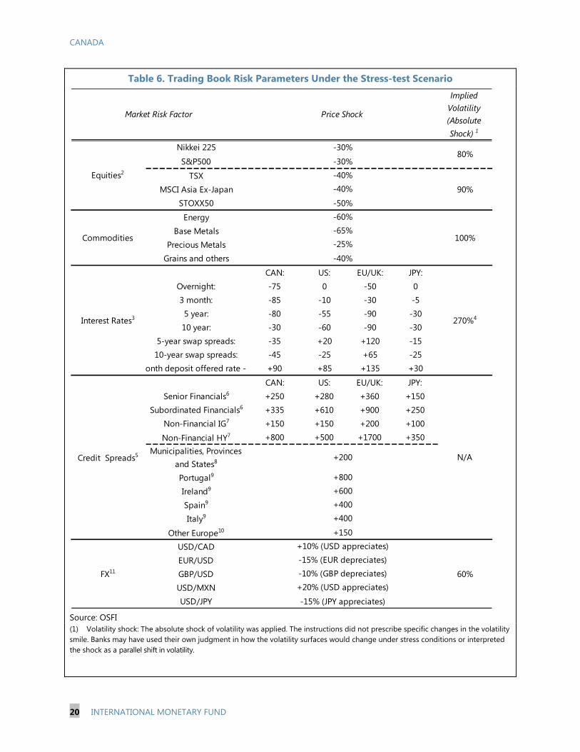
Market risk shock in the trading book, AFS securities and OTC derivatives was undertaken to isolate the impact of market risk shocks on the trading book, AFS securities and on CVA on the OTC derivatives by risk factor (equity, interest rate, credit spread, commodity and foreign exchange rate shocks). No inter-risk diversification benefit and no management actions were assumed. The full revaluation was based on shocks specified in Table 6.
Incremental risk charge shock was simulated to calculate the impact of obligor correlations increasing by 25 percent on a relative basis.
Table 5. IRBBB Spreads Under the Stress-test Scenario
Source: OSFI
CANADA
20 INTERNATIONAL MONETARY FUND
Implied Volatility (Absolute Shock) 1
Nikkei 225
S&P500
TSXMSCI Asia Ex-Japan
STOXX50
EnergyBase Metals
Precious MetalsGrains and others
CAN: US: EU/UK: JPY:Overnight: -75 0 -50 03 month: -85 -10 -30 -55 year: -80 -55 -90 -3010 year: -30 -60 -90 -30
5-year swap spreads: -35 +20 +120 -1510-year swap spreads: -45 -25 +65 -25
onth deposit offered rate - +90 +85 +135 +30
CAN: US: EU/UK: JPY:Senior Financials6 +250 +280 +360 +150
Subordinated Financials6 +335 +610 +900 +250Non-Financial IG7 +150 +150 +200 +100
Non-Financial HY7 +800 +500 +1700 +350Municipalities, Provinces
and States8
Portugal9
Ireland9
Spain9
Italy9
Other Europe10
USD/CADEUR/USDGBP/USDUSD/MXNUSD/JPY
Market Risk Factor Price Shock
Equities2
-30%80%
-30%-40%
90%-40%
-50%
Commodities
-60%
100%-65%-25%
-40%
Interest Rates3 270%4
Credit Spreads5 N/A+200
+800+600+400+400
+150
FX11
+10% (USD appreciates)
60%
-15% (EUR depreciates)-10% (GBP depreciates)+20% (USD appreciates)
-15% (JPY appreciates)
Table 6. Trading Book Risk Parameters Under the Stress-test Scenario
Source: OSFI (1) Volatility shock: The absolute shock of volatility was applied. The instructions did not prescribe specific changes in the volatility smile. Banks may have used their own judgment in how the volatility surfaces would change under stress conditions or interpreted the shock as a parallel shift in volatility.

CANADA
INTERNATIONAL MONETARY FUND 21
Table 6. Trading Book Risk Parameters Under the Stress-test Scenario (Concluded) (2) In mapping the general equity shock to individual names, banks could have applied the CAPM model.
(3) For other terms in the yield curves, banks used linear interpolation to derive the respective shocks. Banks should have used their best judgment for other rates/spreads/basis along with the general description of the scenario and the path for financial variables provided in the instructions.
(4) Normalized; this is based on a 1-month at-the-money swaption on a 5yr USD interest rate swap. The shock was assumed to apply to all currencies.
(5) Overlap across categories: Whenever an exposure overlaps across categories, the most conservative shock should have been applied (e.g., a high-yield corporate exposure in Italy should have been stressed using the high-yield spreads).
(6) Financial exposures include commercial and investment banks, financial holding companies, insurers, specialized insurance (monolines), broker-dealers and hedge funds.
(7) All non-financial non-government credit exposures. Structured credit with implicit or explicit government support was subject to that government’s credit spread, if applicable. For example, NHA MBS and U.S. Agency MBS securities wouldn’t be subject to a credit spread shock as Canada and the United States were not subject to credit spread shocks.
(8) Credit spread that applies to municipal, provinces and state government securities, as well as exposures that benefit from an explicit or implicit guarantee from those entities. This spread was applicable across countries.
(9) Spreads are over Germany, based on 2y rates. The same credit spread shock applied across maturities.
(10) Other European countries spread to Germany, based on 2y rates. Supranational and other European national agencies were also subject to the credit spread shocks, including ESM/EFSF securities.
(11) For other crosses, banks could have used information contained in the table of financial variables, by computing the change in the Q3/13 exchange rates versus their starting levels (Q4/12).
Results
35. The results of the BU solvency stress test suggest that while five banks would fall below the Canadian “all-in” supervisory threshold by 2015, the capital shortfall would be small (Figures 25 and 31-end of text). System-wide “all-in” CET 1 declines by 180 basis points during the recession (2013-2015) in comparison to 2012 “all-in” CET1, and 430 basis points in comparison to 2015 “all-in” CET1 in the baseline (non stress) scenario. All banks would fall below the Canadian “all-in” supervisory threshold in 2016 due to introduction of the D-SIB surcharge with the aggregate capital shortfall of 80 bps. However, four banks would recover above the Canadian “all-in” CET1 threshold of 8 percent in 2017. During the whole stress testing horizon, only one bank would fall below the regulatory threshold (by 20 bps) in 2017 due to D-SIB surcharge introduction and a convergence of Basel III regulatory ratios to supervisory threshold. Total recapitalization needed to bring all banks to the Canadian “all-in” supervisory threshold peaks at 9 percent of their 2012 gross income in 2016 (Figure 31), or 40 percent of their 2012 net income. This corresponds to 0.7 percent of 2016 nominal GDP.
36. The results in years of downturn were mainly driven by charges for impairment (Figure 26).
Charges for impairment subtract 150 bps in 2013 from CET1 which is three times higher than in the base year. From 2014, credit losses’ contribution amount to more than 200 bps. An increase in charges for impairment is mainly driven by individual and collective charges for identified

CANADA
22 INTERNATIONAL MONETARY FUND
losses (equal to expected losses) on exposures in the construction and manufacturing sectors and consumer loans in Canada, and business loans in the U.S. These are driven by an increase in default rates and smaller recovery rates during recession.
RWAs have a negative effect on the Common Equity Tier 1 (CET1) capital ratio in the first two years when they reduce the CET1 ratio by 90 bps and 45 bps respectively. An increase in aggregate RWAs in the first two years (11 and 8 percent respectively) is driven by increases in RWAs for credit risk in corporate sector and consumer loans sector (other retail). This probably reflects lower credit quality and downgrades, consistent with higher default rates of those sectors. RWAs in the last three years are stable, which likely reflects higher growth in exposures offset by an increase in credit quality. RWAs for market risk increased by 22 percent in the first years. However, given its size in the total RWAs (around 5 percent) this increase did not have a big negative impact on CET1.
Dividend distribution has a quantitative impact similar to that of the increase in RWAs during the first two years12. However, the impact of dividend distributions throughout the stress horizon stays negative. This is a consequence of positive net incomes. While still positive, net income drops significantly by 2015 in comparison to the base year and is mostly driven by a large increase in charges for impairment. Net interest income goes down mainly due to lower demand for credit, whereas non-interest income and non-interest expense do not move much by 2015 but increase by the end of the period, reflecting economic recovery. Trading income had a positive impact on the capital position since banks did not experience material losses in their trading book during the stress period.
37. Sensitivity analysis suggests that a single shock would not entail large losses. Sensitivity analyses were performed against an interest rate shock in the banking book, market risk shock and incremental risk charge shock. The results show that:
Interest rate shock in the banking book: an aggregate loss from materialization of the interest rate risk would correspond to around 5 percent of CET1 capital.
Market risk shock in the trading book, AFS securities and OTC derivatives: the aggregate loss rate (loss over mark-to-market value of portfolio) on trading book and AFS securities was equal to 1.8 percent and 1.6 percent respectively. Both losses, which are mostly driven by equity and credit spreads amount to less than 10 percent of CET1 capital. While CVA on the OTC derivatives would double, the impact on the capital position would be small as the total loss is less than 1 percent of total CET1 capital.
12 The impact might be larger if all bank applied the CCB dividend distribution rule consistently. A consistent application of the CCB rule was done by OSFI (on an annual basis). The negative impact was larger and ranged from 27 bps to 101 bps across banks in 2015.

CANADA
INTERNATIONAL MONETARY FUND 23
INTEREST INCOME
INTEREST EXPENSE
BENCHMARK:
NON-INTEREST INCOME EXCLUDING TRADING Impact of point-in-time PDs
NON-INTEREST EXPENSES (balance sheet)
SENSITIVITY:TRADING INCOME(including change in net unrealized gains on AfS securities and Derivatives designed as cash flow hedges ) Impact of loss-given default
Impact of asset correlationFOREIGN CURRENCY TRANSLATION
Impact of regulatory RWAs
CHARGE FOR IMPAIRMENT
TOTAL COMPREHENSIVE INCOME
Capital (t+1) = RWAs
RISK WEIGHTED ASSETSINCOME STATEMENT
IRB formula (credit risk)
Capital (t) + total comprehensive income - dividends
Lending rates x Loans
Deposit rates x Deposits
Nominal GDP
Balance sheet
TSX, Nominal GDP
CAD/USD exchange rate
PD x LGD x Exposure
Incremental risk charge shock: the change in RWAs for IRC ranges from -10 percent to 50 percent across banks. However, the size of IRC RWAs is very small so that even the largest increase of these RWAs would result in only a marginal decline of CET1.
B. IMF Top-down Stress Test
38. The IMF top-down stress testing approach followed the balance sheet based stress testing spreadsheet model similar to Schmieder et al (2011). This approach assesses solvency of individual banks through changes in net income and risk-weighted assets (Figure 1) and is a cornerstone of FSAP stress testing and continues to be applied in the largest, most systemic financial systems (e.g., in U.K., U.S., France, Germany). While this approach resembles the bottom up stress test, the framework was based on “economic” measures of solvency, both for capital and for RWAs. The charge for impairment was assumed to be equal to expected losses, with the assumption that net loan loss reserves serve as the first line of defense against credit losses. RWAs for credit risk were calculated by Basel II asset classes using the IRB formula. However, an economic definition of credit RWAs was used where different approaches to economic RWAs were examined. In the benchmark case, TTC PDs were replaced by the PDs used for the calculation of expected losses. In the sensitivity analysis, RWAs were calculated using regulatory parameters but were also stress-tested against positive asset correlation and stressed LGDs used in calculation of expected losses in the BU test.
Figure 1. IMF Top Down Approach
CANADA
24 INTERNATIONAL MONETARY FUND
Credit losses 39. The key element of the solvency framework includes the computations of credit losses under stress. Credit losses, which will enter the income statement as charge for impairment, are defined as expected losses. These losses are calculated using PIT PDs, downturn LGDs and exposure at default by economic sector over the scenario horizon. It is assumed that expected losses are fully provisioned meaning that the full amount of expected losses enters the income statement and that losses cannot be distributed over time. However, we also assume that loan loss reserves (net of realized losses on 2012 NPLs)13 serve as the first line of defense against credit losses.14
Ideally, downturn LGDs by economic sectors would be used to calculate expected losses. Since these data do not exist,15 in the first step downturn LGDs by Basel II asset classes, provided by OSFI, were mapped into LGDs by new Basel II asset classes (Table 7).16
In the second step, the central bank projections of delta PDs17 by economic sectors (see Table 3 for the sectoral breakdown of banks’ credit portfolio and a mapping between economic sectors and PDs) were applied to base year (2012) bank-specific, PIT PDs by economic sectors supplied by banks in the BU exercise.18
In the third step, PIT PDs by economic sectors were mapped into PIT PDs by new Basel II asset classes.
In the fourth step, exposures by economic sectors were mapped into exposures by new asset classes (calculated using the same mapping from economic sectors to new asset classes).
13 Realized losses on 2012 NPLs are calculated as a product of 2012 stock of NPLs and weighted average LGDs. 14 Assuming that loan loss reserves can cushion credit losses does not have a big impact on the credit position of the banks due to an offsetting impact of the dividend distribution rule-- assuming that loan loss reserves cannot serve as a first line of defense for credit losses would increase the charge for impairment and reduce net income but at the same time decrease a dividends payout. 15 Bank reported stressed LGDs by economic sectors for the BU test. However, two banks’ LGDs were significantly lower than downturn LGD provided by OSFI. While this is the reason why stressed LGD were not used in the benchmark case, in the sensitivity analysis we also use stressed LGDs reported by banks to calculate both expected losses by economic sectors and RWAs for credit risk. 16 Original Basel II asset classes were not used since there is no straightforward way to map business exposures by economic sectors into corporate and SMEs, or retail exposures by economic sectors into other retail excluding Qualifying Revolving Retail and Qualifying Revolving Retail. Therefore, new Basel II asset classes combine corporate and SMEs into a new asset class, “corporates” and other retail excluding Qualifying Revolving Retail and Qualifying Revolving Retail were combined in “other retail.” 17 Sectors include agriculture, construction, manufacturing, mortgage, retail and wholesale. 18 This will make expected losses smaller then if we would apply projected delta PDs to through-the cycle, sectoral, bank specific PDs.

CANADA
INTERNATIONAL MONETARY FUND 25
Finally, expected losses by asset classes19 were calculated using PIT PDs, downturn LGDs and exposures by new Basel II asset classes. In the sensitivity analysis, we use PIT PDs by economic sectors, stressed LGDs by economic sectors reported by banks for the BU test and exposure at default by economic sectors to calculate expected losses by economic sectors.
Exposure at default is taken from the BU exercise. It takes into account credit risk mitigation (i.e., by reclassifying exposures according to the guarantor exposure class, including for certain OTC derivatives and repo style transactions by reducing exposures by collateral). Exposures account for an estimate of potential future changes to that credit exposure (undrawn commitments).
19 Calculating expected losses using weighted averages of PDs and LGDs instead of PDs and LGDs by economic sectors will introduce some overestimation of expected losses (as product of weighted averages of PDs and LGDs and sum of EADs is always equal or greater than sum of products of individual PDs, LGDs and EADs).

CANADA
26 INTERNATIONAL MONETARY FUND
CORPORATES Corporates excluding SME CanadaSME Accommodations
AgricultureConstructionManufacturingWholesaleUSBusiness loansCommercial real estateEuropeBusiness loansLatin America and CarribeanBusiness loansRest of the worldBusiness loans
SOVEREIGN Sovereign Canadian governmentsUS GovernmentsEuro GovernmentsLA GovernmentsROW GovernmentsCanada other (insured mortgages)US other (insured mortgagages)
BANKS Banks Canada Financial institutions
RESIDENTIAL MORTGAGES Residential mortgages Canada including helocs including HELOCs Residential mortgages (uninsured)
HELOCs (uninsured)USResidential mortgages (uninsured)HELOCs (uninsured)Latin America and CarribeanResidential mortgages (uninsured)Rest of the worldResidential mortgages (uninsured)
OTHER RETAIL Other Retail excl. QRR CanadaQualifying Revolving Retail Consumer loans
USConsumer credit card loansOther consumer loansEuropeConsumer loansLatin America and CarribeanConsumer loansRest of the worldConsumer loans
SMALL BUSINESS LOANS SBEs Canada Small business loans
NEW BASEL II asset classes Basel II asset classes Economic sectors
Table 7. Mapping Basel II Asset Classes and Exposures by Economic Sectors into New Basel II Asset Classes

CANADA
INTERNATIONAL MONETARY FUND 27
RWAs 40. RWAs for credit risk under stress were calculated for individual banks using Basel II IRB formula. The formula translates downturn LGDs, changes in PDs, changes in assets correlation and the maturity adjustment parameter into stressed RWAs in economic terms. “Standardized exposures” were added to “IRB exposures” to calculate total exposures by asset classes. To project RWAs for credit risk over the stress horizon, percentage changes in calculated RWAs were applied to the base year, realized RWAs.20 Projected levels of calculated RWAs were used in a calculation of capital requirements under the two scenarios. Forecast of changes in PIT PDs were taken from the BoC and applied to PIT PDs in the base year that the banks reported for the BU test. The dynamics of exposures by Basel II asset classes were made consistent with the dynamics of exposures by economic sectors using the mapping from the Table 7.21 Downturn LGDs and average effective maturity were provided by OSFI from the regulatory returns. For the calculation of the RWAs, it was assumed that the assets compositions reflect the dynamic of assets reported by banks in the BU exercise. It was also assumed that banks will not replace maturing loans with different assets that have a different risk weight. Moreover, no RWA optimization was assumed.
41. In the sensitivity analysis, RWAs for credit risk were tested against different assumptions of the IRB formula parameters. PIT PDs, downturn LGDs, asset correlation (assumed to move inversely with PDs), maturity adjustment (assumed to move with PDs as in Basel II) and effective maturity constitute the set of parameters used to calculate RWAs for credit risk. Sensitivity analyses were performed with respect to different LGDs (that follow dynamics of LGDs reported by banks in the BU), positive asset correlation (explained below) and use of regulatory calibration of the parameters where, instead of PIT PD, TTC PDs are used. Moreover, in this scenario loan loss reserves were assumed not to serve as the first line of defense against credit losses.
42. Data constraints on PDs for Basel II asset classes precluded the calculation of RWAs on a Basel II asset class level.22 To compute changes in sectoral RWAs we would ideally need data on sectoral (Basel II asset classes) PIT PDs, sectoral downturn LGDs, sectoral asset correlations (a function of PDs or fixed as in Basel II formulas), maturity adjustment (a function of PDs as in Basel II formulas) and sectoral effective maturity. All parameters were available to the FSAP team except PIT PDs, which were available for economic sectors only. Therefore mapping of economic sectors into Basel II classes (Table 7) was devised to construct new Basel II asset classes (first column of Table 7) where each asset class will have an effective maturity, a downturn LGD calculated as a weighted average of the same items of the corresponding Basel II asset classes from the regulatory returns (second column of Table 7). On the other hand, PDs of new Basel II asset classes will be calculated as weighted averages of PDs by 20 Note that we have necessary data to calculate percentage change of RWAs in 2013 using calculated levels of RWAs in 2013 and 2012. 21 Replacing the credit growth parameters for EAD with the BoC model implied growth rate does not affect the results significantly. 22 Data constraints on sectoral effective maturity and downturn LGDs, which we have for Basel II asset classes only, preclude the calculation of RWAs changes on an economic sectoral level.
CANADA
28 INTERNATIONAL MONETARY FUND
economic sector (third column of Table 7). This allows the calculation of changes in RWAs by asset classes as a function of a sector specific PD, a downturn LGD, asset correlation and maturity adjustment (for non-retail sectors). At the same, the mapping between economic sectors and Basel II asset classes ensures that RWAs and expected losses are consistently calculated using the same parameters.
43. Basel II formulas were used to assess the impact of changes in asset correlations on RWAs. Basel II regulatory formulas, which were used in the benchmark case, assume that average asset correlation decreases with PDs.23 However, some studies provide economic arguments against the negative correlation and suggest that the relationship is more likely to be an increasing one (Moody’s, 2009; Fitch 2008; Laurent, 2004; Schmieder et al, 2011). In order to simulate this intuitive relationship during the stress scenario the negative impact of an increase in PDs on asset correlation was replaced by the positive impact (by the same amount i.e., only the sign has changed) as part of the sensitivity analysis. This positive impact of increasing PDs on asset correlation increased RWAs for credit risk.
44. RWAs for other exposures were taken from the BU test. Since there is no easy and straightforward way of modeling the rest of the RWAs components, credit risk RWAs for trading book,24 equity and securitization as well as RWAs for market and operational risk were taken from the BU exercise.
Income statement
45. Simple econometric models (satellite models) were used to translate macroeconomic scenarios into projections of most income statement items. Using estimated models, various components of the income statement were projected over the stress testing horizon. The satellite models incorporated as explanatory variables the core macroeconomic and financial variables from the scenarios as determined jointly by the authorities and the IMF FSAP team. In cases where a reasonable relationship between components and explanatory variables was not found, a standardized set of common, behavioral assumptions was applied across all banks.
46. The following models and assumptions were used to project income statement items:
The charge for impairment was assumed to equal credit losses/expected losses and calculated using downturn LGD provided by OSFI, PDs provided by banks following instructions from the BoC on changes in PDs and exposure at the default reported by banks for the BU stress testing exercise.25
23 The asset correlation formula of Basel II is based on a single (systemic) risk factor model where it is assumed that higher PDs are driven by individual risk which implies low correlation with other borrower’s assets. This negative correlation was justified by the desire to reduce procyclicality of the RWAs. 24 Trading book in Basel II asset classes does not have a corresponding item in economic sectors. RWAs for equity and securitization exposures are not calculated using the IRB formula. 25 More details on how credit losses were calculated are provided in paragraph 39.

CANADA
INTERNATIONAL MONETARY FUND 29
Interest income was projected using panel regression of the y-o-y growth rate of interest income on the y-o-y growth rate of a product of total loans and loan interest rates26 as an explanatory variable (see Figure 18 in Appendix) and fixed effects. Projections of loans and interest rates were taken from the scenarios.
Interest expenses were projected using panel regression of the y-o-y growth rate of interest expenses on the y-o-y growth rate of a product of total deposits and deposit interest rates27 as an explanatory variable (see Figure 19 in Appendix) and fixed effects. Deposits were assumed to grow at y-o-y growth rate of loans (Figure 23 in Appendix).28 Interest rates follow the dynamics of the interest rates projected by the authorities consistent with the scenarios.
Non-interest income that excludes trading income was projected as an average share of nominal GDP (Figure 21 in Appendix) in the last 5 years. Projection of nominal GDP was taken from the scenarios.
Non-interest expense was projected as an average share of the balance sheet, assuming that balance sheet growth rate is equal to the growth rate of loans (Figure 24 in Appendix) and the projection of loans was taken from the scenarios.
Trading income: in addition to OSFI’s trading income29 and realized gains/losses on instruments held for “other-than-trading purposes” that affect the income statement, the FSAP team’s definition of trading income also included items that affect comprehensive income30: (i) changes in unrealized gains/losses on available-for-sale (AFS, net of reclassification to earnings) and (ii) derivatives designed as cash flow hedges (unrealized gains and losses net of reclassification to earnings).31 Y-o-y growth rate of trading income was modeled using panel regression on
26 Loan interest rates are weighted average of consumer, business and mortgage interest rates adjusted for bank specific structure of the loan portfolio. 27 Deposit interest rates are weighted average of short-term and long-term deposits rates adjusted for bank specific structure of the deposit portfolio. 28 The assumption that deposits grow in line with nominal GDP was also tried. However, given the time series properties of the data (correlation between growth rates of loans and deposits is 0.64 whereas a correlation between the growth rate of deposits and the growth rate of nominal GDP is 0.23) it was assumed that deposits growth is equal to loans growth. 29 On an aggregate level, a major part of trading losses in 2008 occurred in the first half of that year. This was due to CIBC losses driven largely by charges on credit protection purchased from financial guarantors (CIBC losses account for 95 percent of total banking sector trading losses in 2008). The other five banks reported losses in the last quarter of 2008. In general, trading income seems to lead the nominal GDP growth and TSX composite index. 30 Changes in unrealized gains/losses on AFS securities, derivatives designed as cash flow hedges and foreign currency translation that affect comprehensive income are not accounted in the income statements but directly in the capital reserves accounts (cumulative foreign exchange translation and unrealized losses on AFS equities reported in OCI). However, from an economic point of view these items will have the same effect on the banking sector solvency, whether they are in the income statement or part of comprehensive income. 31 Publicly available data for AFS unrealized gains and derivatives designed as cash flows are available from 2007. During the fourth quarter of 2008 the CICA amended accounting and reporting rules applicable to financial instruments. As a result of the amendments, some banks elected to transfer certain securities from their trading
(continued)
CANADA
30 INTERNATIONAL MONETARY FUND
y-o-y growth rates of Toronto Stock Exchange (TSX) Index and nominal GDP32 as explanatory variables (Figure 26). Dummy variables for a 2007 structural break were included due to the addition of comprehensive income items to trading income, as well as dummy variables for CIBC losses which are expected not to be repeated in the future. Projections of both nominal GDP and TSX were taken from the scenarios. When projecting trading income, the fact that trading income as a share of GDP (or balance sheet) was constant except during the crisis was taken into account.
Foreign currency translation (changes in unrealized gains and losses net of hedging activities), that affect CET1 directly were projected using panel regression of y-o-y growth rate of FX valuations on y-o-y growth rate of the CAD/USD exchange rate.33 Projections of the CAD/USD exchange rate were taken from the scenarios.
Taxes were set at the effective tax rate (share of net income) in 2012 in case of positive net income and zero otherwise.
Other stress testing components
Balance sheet projection
47. The balance sheet asset allocation was assumed to be constant under all scenarios, with maturing exposures assumed to be replaced with similar ones. Banks’ balance sheets were assumed to grow in line with total loans (Figure 24 in Appendix). For the purpose of projecting the income statement items, loan growth was assumed to be equal, for all banks, to growth of total credit. The loan growth rate was taken for the scenarios.34 Asset disposals and acquisitions over time were not considered.
Dividend payout
48. Dividend payouts were payable out of the current year’s profit using the adjusted IMF capital conservation rule. Dividends were assumed to be paid out of current period net income after taxes by banks that were in compliance with supervisory capital requirements (i.e., Canadian
portfolio to their available-for-sale portfolio. This suggests that modeling trading income and AFS valuation changes should be done together. Derivatives designed as hedges did not have a large impact on comprehensive income. 32 Both variables were included as lead variables. 33 In the 2008 downturn, trading losses and negative pressures on capital due to unrealized losses on ASF securities were offset by depreciation of the Canadian dollar. On the other hand, during the recovery period (since 2009) appreciation of the Canadian dollar had a negative impact on capital. 34 We experimented with loan growth rates reported by banks in the BU exercise. The results, with respect to net interest income and net non-interest income, did not change much. The reason is that for a bank that has higher growth rate of loans than the growth rate of total loans, its net income would increase marginally since the loan growth rate was assumed to be equal to deposits growth rate. On the other hand, higher loan growth would imply higher non-interest expense (which depends on the balance sheet dynamics) which would offset increases in the net interest income.

CANADA
INTERNATIONAL MONETARY FUND 31
Capital ratio ("all-in" CET 1): 2013-2015 Capital ratio ("all-in" CET 1): 2016-2017 Assumed dividend payout
4.5-5.125 5.5-6.125 0%x Net income (t)5.125-5.75 6.125-6.75 20% x EDPR x Net income (t)5.75-6.375 6.75-7.375 40% x EDPR x Net income (t)6.375-7.0 7.375-8.0 60% x EDPR x Net income (t)
>7.0 >8.0 Effective div. payout rate in 2012 (EDPR)
“all-in” supervisory CET 1 thresholds). A maximum allowed dividend payout was assumed to be equal to the dividend payout ratio (dividends over net income after taxes) in 2012. If a bank fell below the Canadian “all-in” supervisory CET1 threshold of 7 percent (8 percent from 2016 onward) before dividend distribution, it was considered capital constrained and followed a schedule of dividend payouts per Table 8. If a bank fell below the Canadian “all-in” supervisory threshold because of dividend distribution, it was assumed that the bank’s dividend payout would be limited to a level that ensures the supervisory threshold is not breached. This rule applied only if a bank earned a positive net income. If net income was negative it was assumed that there is no dividend payout. If a bank was above the threshold, it paid a maximum-allowed proportion of dividend.
Table 8. Dividends Distribution Schedule
Source: IMF Staff calculation
Results
49. While all banks would fall below the Canadian “all-in” CET1 supervisory threshold during severe economic distress, recapitalization needs would be manageable. The results of the IMF solvency stress test suggest that all banks would fall below the Canadian “all-in” CET1 supervisory threshold by 2015 (Table 11 and Figure 25- end of text). This is expected given banks’ capital position in the base year relative to the supervisory threshold, which incorporates early adoption of both the Basel III thresholds and supervisory adjustments. System-wide “all-in” CET 1 declines by 250 basis points during the recession (2013-2015) in comparison to 2012 “all-in” CET1, or 540 basis points in comparison to 2015 “all-in” CET1 in the baseline scenario. All banks would stay below the Canadian “all-in” CET1 supervisory threshold by the end of the stress horizon and four banks would fall below regulatory threshold in the last two years of the horizon. This is mainly due to the D-SIB surcharge imposed in 2016, and despite a recovery in banks’ capital position from 2016 (by 60 bps by 2017). Recapitalization needed to bring all banks to the Canadian “all-in” CET1 supervisory threshold peaks at 32 percent of their 2012 gross income in 2016 (Figure 31), or around 150 percent of their 2012 net income - which corresponds to 2.5 percent of 2015 nominal GDP. Recapitalization needs to bring the banks to the regulatory threshold also peak in 2016 but are five times smaller.
50. The results in years of downturn were mainly driven by the increases in RWAs and in charges for impairment (Figure 26).

CANADA
32 INTERNATIONAL MONETARY FUND
Canada64%
United States24%
Euro Area4%
Latin America and Carribean
7%
Rest of the World
1%
Accommodations
11%
Construction15%
Manufacturing17%
Consumer loans35%
Other15%
Small business loans7%
In the first year, RWAs for credit risk play the major role in the deterioration of CET1 ratios. Aggregate RWAs for credit risk increase by 44 percent in the first year and further by 18 percent and 7 percent in the second and third years. The large increase in the first year is mainly due to an increase in default rates due to the start of a recession particularly due to an increase in default rates on exposures to Canadian financial institutions and to the corporate sector in Canada and abroad.
Credit losses start affecting net income (which becomes negative in 2015 and 2016) and therefore the capital position significantly from 2014. The first year’s effect is cushioned by loan loss reserves which are exhausted in the first period of the stress horizon. Credit losses reach their peak at the end of recession, in 2015, when they are more than four times larger than expected losses in 2012 and more than seven times larger than the TTC measure of expected loss (i.e., the product of TTC PDs, downturn LGDs and exposures). An increase in credit losses is mainly driven by an increase in default rates and the size of exposures on the corporate sector (mostly the construction sector in Canada and business loans in the U.S.) and consumer loans in Canada (Figure 2). Losses are concentrated in Canada and the U.S. Around 65 percent of losses at their peak (2015) come from Canadian exposures (mostly consumer loans, construction, accommodation, and manufacturing) and around 25 percent from U.S. exposures (mostly business loans). Canada accounts for around 75 percent of exposures while the U.S. accounts for around 15 percent of exposures.
Figure 2. Geographical and Sectoral35 Distribution of Losses and Exposures
Geographical distribution of losses Sectoral distribution of losses in Canada
35 Sectors are BoC economic sectors as defined in Table 3.

CANADA
INTERNATIONAL MONETARY FUND 33
Business loans48%
Commercial real estate
15%
Residential mortgages (uninsured)
8%
HELOCs (uninsured)
8%
Consumer credit card
loans12%
Other consumer
loans9%
Other0%
Business loans59%
Governments6%
Residential mortgages (uninsured)
10%
Consumer loans25%
Figure 2. Geographical and Sectoral Distribution of Losses and Exposures (Concluded)
Sectoral distribution of losses in the U.S. Sectoral distribution of losses in Rest of the World
Source: OSFI
While the cushioning impact of net interest income and non-interest income falls sharply in the first three years due to lower credit demand—reflecting the depressed economic environment—the effect on capital is cushioned by falling non-interest expenses (relative to RWAs). Since trading income, also taking into account realized and unrealized gains/losses, has not been historically a major driver of net income (or comprehensive income), any impact of trading income (negative in 2013 and positive from 2014 onwards) is too small to affect capital positions significantly.36 The modest negative impact of dividend distribution is felt in the first year only, due to the capital conservation rule kicking in from 2014 onwards.
51. Sensitivity analysis suggests that, under the most severe parameterization, i.e., of positive asset correlation, the decline in banks’ capital adequacy would be significantly larger. Sensitivity analyses (Figure 3) were performed with respect to different LGDs (that follow dynamics of LGDs reported by banks in the BU), positive asset correlation and a regulatory risk parameter input where, instead of PIT PDs, TTC PDs were used. The results of sensitivity analysis shows that:
Using the intuitive assumption that asset correlation moves in the same direction as PDs generates the worst outcome. The system-wide “all-in” CET1 ratio would fall by 450 basis points during the economic downturn (2013-2015) relative to the base year CET1 ratio or 740 basis points in comparison to 2015 CET1 in the baseline scenario. Most banks would fall significantly below the Canadian “all-in” CET1 supervisory threshold by end-2013. By comparison, the same banks
36 On an aggregate level, a major part trading losses in 2008 of Can$7.1 billion was due to CIBC losses only, driven largely by charges on credit protection purchased from financial guarantors. This loss was assumed not to happen during the stress period.

CANADA
34 INTERNATIONAL MONETARY FUND
would go below the regulatory threshold only in last two years of the stress horizon in the benchmark case reported above.
Using LGDs dynamics from the BU test would be also severe—the aggregate “all-in” CET1 ratio would fall by 390 basis points over the first three years.
A scenario where regulatory parameters were used in the calculation of RWAs for credit risk and loan loss reserves were not considered as the first line of defense against the credit losses was benign.37 It resulted in a decline of the system-wide “all-in” CET1 ratio by 100 basis points over the five year stress horizon. Even though regulatory parameters were used, as in the BU exercise, the results with respect to RWAs are not comparable since banks took into account credit quality migration under stress which is something that was not possible to do in the ToD exercise.
37 Assuming that loan loss reserves cannot cushion credit losses has the positive impact on the system-wide CET1 of 20 bps only.
CANADA
INTERNATIONAL MONETARY FUND 35
0.0
1.0
2.0
3.0
4.0
2012 2013 2014 2015 2016 2017IMF top downBottom upIMF top down (TTC PDs, regulatory RWAs)
20.0
25.0
30.0
35.0
2012 2013 2014 2015 2016 2017IMF top downBottom upIMF top down (stressed LRDEs)
3.0%
4.0%
5.0%
6.0%
7.0%
8.0%
9.0%
10.0%
2012 2013 2014 2015 2016 2017IMF top downIMF top down (positive asset cor)IMF top down (regulatory RWAs)IMF top down (stressed LRDEs in RWAs and EL)Supervisory "all-in" thresholdRegulatory threshold
Figure 3. IMF ToD Solvency Stress Test Results—Sensitivity Analysis
CET1 ratios with different RWAs for credit risk
Weighted average PDs Weighted average LGDs
Sources: OSFI, BoC, IMF Staff calculations

CANADA
36 INTERNATIONAL MONETARY FUND
C. OSFI Top-down Stress Test
52. The OSFI stress test followed a similar logic to the bottom-up and the IMF approach. Income statement items, excluding the charge for impairment, were calculated based on corresponding balance sheet items which were projected using variables in the stress scenario. Credit losses were projected using a calibrated law of motion for the loan loss reserves. In the benchmark case, RWAs for credit risk were calculated using risk weights from the previous year’s bottom-up stress scenario. The OSFI ToD module was performed against the stress scenario only.
Credit losses
53. Credit losses were calculated as charge for impairment consistent with regulatory standards. The charge for impairment was projected using an algorithm (Box 1) that simultaneously projects the balance sheet loan book, performing, non-performing and impaired loans and loan loss reserves using regulatory formulas.
RWAs
54. RWAs for credit risk were projected by using risk weights and exposures consistent with the stress scenario. To calculate RWAs for credit risk, exposures by Basel II asset classes were projected to grow in line with performing loans and risk weights were calculated by dividing RWAs and exposure for each asset class reported by banks in the 2012 OSFI stress test.38 In the sensitivity analysis, RWAs were calculated by asset classes using IRB formulas and regulatory parameters of IRB formulas—the exposures and downturn LGDs were taken from the BU exercise, TTC PDs were updated by using PIT PDs over the stress horizon. It was assumed that there are no standardized exposures.
55. RWAs for market and operational risk were projected using OSFI’s internal models. While RWAs for market risk during good times (positive GDP growth) were assumed to be the same as in the base year, RWAs in bad times (negative GDP growth) were calculated by doubling the SVaR. The calculation of RWAs for operational risk followed the standardized approach for operational risk which depends on gross income.
Income statement
56. Income statement was projected using corresponding balance sheet items projected consistent with the stress scenario. After projecting the whole balance sheet (see Balance Sheet section for more details), income statement items were projected as a function of corresponding balance sheet items. In particular:
Charge for impairment was projected as described in Box 1.
38 Since the 2012 OSFI stress test was a three year stress test, risk weights of the last year of 2012 stress test were used for the last two years of the current stress test.

CANADA
INTERNATIONAL MONETARY FUND 37
Interest income was projected using projected interest rates (on business, personal, mortgage and other loans) and corresponding assets consistent with the stress scenario. The imputed interest rates were calculated by dividing interest income to corresponding assets in the base year. Only the interest rate on mortgage loans was adjusted for an assumed fall in mortgage interest rates. Other interest rates were assumed to be constant throughout the stress horizon and equal to the imputed interest rate for the base year.
Interest expense was projected using projected interest rates (on subordinated debt, deposits) and corresponding liabilities consistent with the stress scenario. The interest rates were calculated by dividing interest expenses to corresponding liabilities in the base year. Only the interest rate on subordinated debt was adjusted for an assumed fall in subordinated debt interest rates. Other interest rates were assumed to be constant throughout the stress horizon and equal to the imputed interest rate for the base year.
Non-interest income was projected by multiplying the ratio of non-interest income (fees, insurance income) to other assets in the base year and projected other assets.
Non-interest expenses were projected by multiplying the ratio of non-interest expense (salaries, premises, other expenses) to total assets in the base year and projected total assets.
Trading income was projected by multiplying the ratio of trading income to securities holdings in the base year and projected stock of securities. While for the first stress year, the ratio was set to the average loss observed in the last 10 years, in the subsequent years it was set to the smallest trading income (excluding trading losses) over the same period. Gains/losses on instruments held for other than trading purposes were not part of trading income but were included in other non-interest income. Unrealized gains/losses were not explicitly projected.
Taxes were set at the effective tax rate (share of net income) in 2012 in case of positive net income and zero otherwise.
Non-controlling interest were added to after-tax income and were assumed to change in line with net income before taxes
Other stress testing elements
Balance sheet projection
57. The balance sheet of each bank was projected in two steps.
First, the loan book and deposits were projected. The loan book consists of net business loans,39 net personal (consumer) loans and net mortgage loans where net loans were defined as gross performing and gross impaired loans minus loan-loss reserves. For each of these components of
39 Business loans include all loans that are not personal and mortgages. Personal loans include personal loan plans, credit cards and other personal loans. Mortgage loans include insured, uninsured, residential and non-residential loans.

CANADA
38 INTERNATIONAL MONETARY FUND
net loans, and for each loan type, projections over the stress horizon were made using the algorithm described in Box 1. Deposits were assumed to grow in line with nominal GDP.
Second, the ratio of other balance sheet items and loans or deposits was calculated for the base year. The ratio, which was held constant throughout the stress horizon, was multiplied by loans (for customers’ liabilities, other assets, repos, derivatives) or deposits (cash, securities, acceptances, subordinated debt, and other liabilities) to project the rest of the balance sheet items.
Box 1. OSFI Algorithm to Project Loan Book
To project the loan book, for each loan type (business, personal, mortgage) OSFI used the following algorithm: Gross loans in period t+1, , were projected using gross loans in period t, , and a nominal growth rate, , that was provided by the BoC for the stress scenario:
Loans that will default in t+1, , were projected using performing loans in period t, , and PDs in period t+1 where delta PDs, , were calculated as weighted averages of delta PDs
provided from the BoC, , where weights correspond to exposures reported by banks in the BU exercise; PDs in the base year were derived using historical data (2003-2012) of defaulted loans (equal to the change in impaired loans and net write-off) and performing loans:
The net write-offs in t+1, , was projected based on gross impaired loans in period t, , and calibrated write-offs ratio, ∗: ∗. This ratio was calibrated using base
year data on net write-offs and impaired loans and would be recalibrated if the algorithm resulted in negative impaired loans. The new recalibration of the ratio would be such that write-offs are equal to defaulted loans.
Having write-offs and defaulted loans in t+1, gross impaired loans in period t+1 were calculated as the sum of impaired loans in period t and defaulted loans and net write-offs in t+1:
/ ∗. Write-offs were adjusted for the proxy for the LGD, ∗,-- a ratio of loan loss reserves in t+1 and impaired loans in t+1-- which was calibrated using LGDs reported by banks in 2012 OSFI stress testing exercise. In some cases, this LGD proxy can be negative or higher than 100 percent (since OSFI’s approach uses both specific and collective allowances, and includes drawn and undrawn exposures).
Loan loss reserves in period t+1, , were projected using the calibrated proxy for the LGD and impaired loans in t+1: ∗
Charge for impairment in t+1, , was then calculated from the law of motion for loan loss reserves (loan loss reserves in t+1 minus loan loss reserves in t plus net write-offs in t+1):
Performing loans in t+1, , were calculated as gross loans in t+1 minus loan loss reserves t+1:
CANADA
INTERNATIONAL MONETARY FUND 39
Dividend payout
58. Dividends payout followed the same rule as in the BU exercise (Table 4) but on an annual basis. If a bank was not capital constrained, dividends were paid in the amount consistent with a dollar per share amount in the base year. However, the capital conservation rule kicked in when a bank was considered capital constrained i.e., when the CET1 ratio was below the Canadian “all-in” supervisory threshold. In that case, year-end CET1 was used to determine how much of the net income from the previous period has to be conserved next period.
Results
59. OSFI’s solvency stress testing results suggest that five banks would fall under the Canadian “all-in” CET1 supervisory threshold by the end of the third year. The results in the downturn period (2013-2015) are similar to BU results. The system-wide “all-in” CET1 ratio in the OSFI ToD model declines by 200 basis points by 2016 in comparison to the 2012 level, with no banks staying above the Canadian “all-in” CET1 supervisory threshold throughout this period. By the end of the recovery period, all banks fall below the Canadian “all-in” CET1 supervisory threshold of 8 percent and two banks fall below the regulatory threshold which is mostly due to introduction of DSIB surcharge and convergence of the regulatory threshold to “all in” metric. Recapitalization needed to bring all banks to the Canadian “all-in” supervisory threshold peaks at 20 percent of their 2012 gross income in 2016 or 90 percent of their 2012 net income which corresponds to 1.5 percent of 2016 nominal GDP (Figure 31).
60. The results in years of downturn were mainly driven by RWAs, charges for impairment and dividends (Figure 32).
RWAs have the largest negative impact on the CET1 ratio in the first year due to an increase of RWAs for credit risk equal to almost 20 percent. In the following years RWAs are mostly stable and do not affect the capital positions of the banks.
While charges for impairment have a similar impact on the CET1 ratio in the first year, they are the most important driver of the solvency ratio in the following years. This is mostly due to an increase in losses on business loans driven by a large increase in default rates.
Realized dividend distribution has a modest negative impact on the capitalization of the banks throughout the stress test horizon. This is due to offsetting positive net income, and reduction on non-interest expenses, accompanied by a significant fall in net interest income over the whole horizon, a one-time fall on non-interest income and trading income in the first year, and a large increase in charges for impairment. Dividends under the capital conservation rule were materially lower than dividends paid out in the base year.
D. Reconciliation of Results
61. Differences in the three sets of results are attributable to the different approaches of modeling RWAs and income statement items and the scope of charge for impairment. While in the stress scenario, results of the IMF ToD exercise are consistent with the BU exercise there are a number of differences across the three approaches (Table 9) that make the results diverse. In particular:
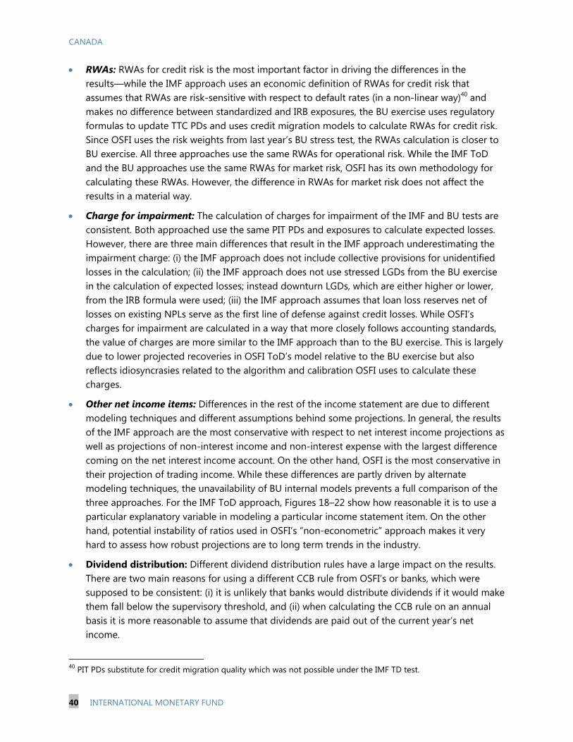
CANADA
40 INTERNATIONAL MONETARY FUND
RWAs: RWAs for credit risk is the most important factor in driving the differences in the results—while the IMF approach uses an economic definition of RWAs for credit risk that assumes that RWAs are risk-sensitive with respect to default rates (in a non-linear way)40 and makes no difference between standardized and IRB exposures, the BU exercise uses regulatory formulas to update TTC PDs and uses credit migration models to calculate RWAs for credit risk. Since OSFI uses the risk weights from last year’s BU stress test, the RWAs calculation is closer to BU exercise. All three approaches use the same RWAs for operational risk. While the IMF ToD and the BU approaches use the same RWAs for market risk, OSFI has its own methodology for calculating these RWAs. However, the difference in RWAs for market risk does not affect the results in a material way.
Charge for impairment: The calculation of charges for impairment of the IMF and BU tests are consistent. Both approached use the same PIT PDs and exposures to calculate expected losses. However, there are three main differences that result in the IMF approach underestimating the impairment charge: (i) the IMF approach does not include collective provisions for unidentified losses in the calculation; (ii) the IMF approach does not use stressed LGDs from the BU exercise in the calculation of expected losses; instead downturn LGDs, which are either higher or lower, from the IRB formula were used; (iii) the IMF approach assumes that loan loss reserves net of losses on existing NPLs serve as the first line of defense against credit losses. While OSFI’s charges for impairment are calculated in a way that more closely follows accounting standards, the value of charges are more similar to the IMF approach than to the BU exercise. This is largely due to lower projected recoveries in OSFI ToD’s model relative to the BU exercise but also reflects idiosyncrasies related to the algorithm and calibration OSFI uses to calculate these charges.
Other net income items: Differences in the rest of the income statement are due to different modeling techniques and different assumptions behind some projections. In general, the results of the IMF approach are the most conservative with respect to net interest income projections as well as projections of non-interest income and non-interest expense with the largest difference coming on the net interest income account. On the other hand, OSFI is the most conservative in their projection of trading income. While these differences are partly driven by alternate modeling techniques, the unavailability of BU internal models prevents a full comparison of the three approaches. For the IMF ToD approach, Figures 18–22 show how reasonable it is to use a particular explanatory variable in modeling a particular income statement item. On the other hand, potential instability of ratios used in OSFI’s “non-econometric” approach makes it very hard to assess how robust projections are to long term trends in the industry.
Dividend distribution: Different dividend distribution rules have a large impact on the results. There are two main reasons for using a different CCB rule from OSFI’s or banks, which were supposed to be consistent: (i) it is unlikely that banks would distribute dividends if it would make them fall below the supervisory threshold, and (ii) when calculating the CCB rule on an annual basis it is more reasonable to assume that dividends are paid out of the current year’s net income.
40 PIT PDs substitute for credit migration quality which was not possible under the IMF TD test.
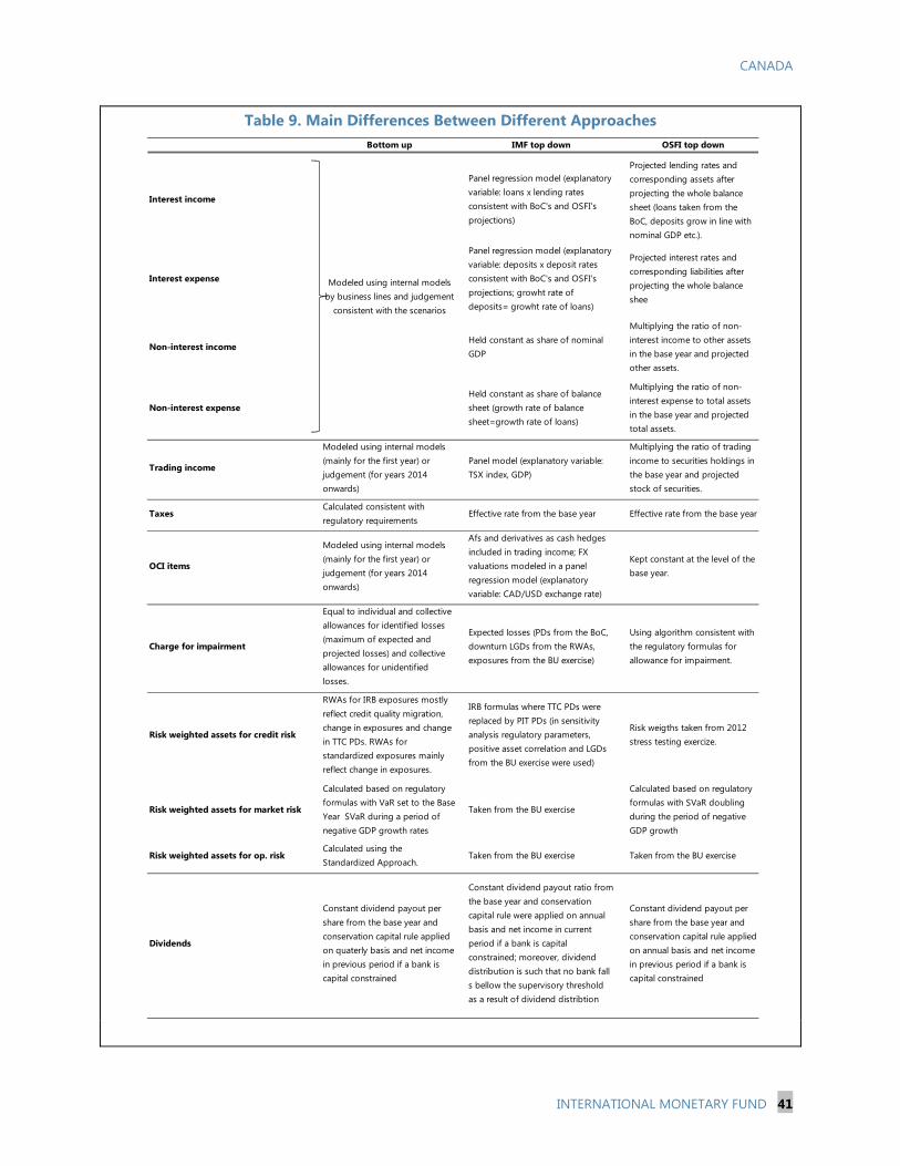
CANADA
INTERNATIONAL MONETARY FUND 41
Bottom up IMF top down OSFI top down
Interest income
Panel regression model (explanatory variable: loans x lending rates consistent with BoC's and OSFI's projections)
Projected lending rates and corresponding assets after projecting the whole balance sheet (loans taken from the BoC, deposits grow in line with nominal GDP etc.).
Interest expense
Panel regression model (explanatory variable: deposits x deposit rates consistent with BoC's and OSFI's projections; growht rate of deposits= growht rate of loans)
Projected interest rates and corresponding liabilities after projecting the whole balance shee
Non-interest incomeHeld constant as share of nominal GDP
Multiplying the ratio of non-interest income to other assets in the base year and projected other assets.
Non-interest expenseHeld constant as share of balance sheet (growth rate of balance sheet=growth rate of loans)
Multiplying the ratio of non-interest expense to total assets in the base year and projected total assets.
Trading income
Modeled using internal models (mainly for the first year) or judgement (for years 2014 onwards)
Panel model (explanatory variable: TSX index, GDP)
Multiplying the ratio of trading income to securities holdings in the base year and projected stock of securities.
TaxesCalculated consistent with regulatory requirements
Effective rate from the base year Effective rate from the base year
OCI items
Modeled using internal models (mainly for the first year) or judgement (for years 2014 onwards)
Afs and derivatives as cash hedges included in trading income; FX valuations modeled in a panel regression model (explanatory variable: CAD/USD exchange rate)
Kept constant at the level of the base year.
Charge for impairment
Equal to individual and collective allowances for identified losses (maximum of expected and projected losses) and collective allowances for unidentified losses.
Expected losses (PDs from the BoC, downturn LGDs from the RWAs, exposures from the BU exercise)
Using algorithm consistent with the regulatory formulas for allowance for impairment.
Risk weighted assets for credit risk
RWAs for IRB exposures mostly reflect credit quality migration, change in exposures and change in TTC PDs. RWAs for standardized exposures mainly reflect change in exposures.
IRB formulas where TTC PDs were replaced by PIT PDs (in sensitivity analysis regulatory parameters, positive asset correlation and LGDs from the BU exercise were used)
Risk weigths taken from 2012 stress testing exercize.
Risk weighted assets for market risk
Calculated based on regulatory formulas with VaR set to the Base Year SVaR during a period of negative GDP growth rates
Taken from the BU exercise
Calculated based on regulatory formulas with SVaR doubling during the period of negative GDP growth
Risk weighted assets for op. riskCalculated using the Standardized Approach.
Taken from the BU exercise Taken from the BU exercise
Dividends
Constant dividend payout per share from the base year and conservation capital rule applied on quaterly basis and net income in previous period if a bank is capital constrained
Constant dividend payout ratio from the base year and conservation capital rule were applied on annual basis and net income in current period if a bank is capital constrained; moreover, dividend distribution is such that no bank fall s bellow the supervisory threshold as a result of dividend distribtion
Constant dividend payout per share from the base year and conservation capital rule applied on annual basis and net income in previous period if a bank is capital constrained
Modeled using internal models by business lines and judgement
consistent with the scenarios
Table 9. Main Differences Between Different Approaches

CANADA
42 INTERNATIONAL MONETARY FUND
Bottom up IMF top down OSFI top down
PDs
For the calculation of expected losses: delta PDs projected by the BoC applied to PIT PDs in the base year; For calculation of RWAs for credit risk: TTC PDs updated for forecasted PDs
For the calculation of expected losses: delta PDs projected by the BoC applied to PIT PDs in the base year; For calculation of RWAs for credit risk: same PIT PDs
For the calculation of expected losses: delta PDs projected by the BoC applied to PIT PDs in the base year. PDs were not used in calculation of RWAs for credit risk
LGDs
Stressed LGDs for the calculation of expected losses projected using internal models; Downturn LGDs used for calculation of RWAs for crdit risk
Downturn LGDs used for calculation of both expected losses and RWAs for credit risk
Stressed LGD for calculation of expected losses calibrated. LGDs were not used in calculation of RWAs for credit risk
Exposures for expected losses
Consistent with BoC forecast. Distributed by economic sectors and include non-defaulted drawn and undrawn commitments, other off-balance sheet items, OTC derivatives an repo style transaction after credit risk mitigation.
Exposures taken from the BU exercise but distributed to new Basel II asset classes.
Exposures growth consistent to BoC projections and distribute across three sectors (personal, business, mortgage)
Exposures for RWAs for credit risk
Consistent with BoC forecast. Distributed by Basel II asset classes. Include IRB and standardized drawn and undrawn commitments, other off-balance sheet items, OTC derivatives an repo style transaction after credit risk mitigation minus defaulted exposures
Exposures by new Basel II asset classes grow in line with exposures by economic sectors.
Consistent with BoC forecast. Distributed by Basel II asset classes.
Sensitivity analysisInterest rate shock in banking book. Market risk shock in trading book.
RWAs for credit risk calculated by assuming: (i) regulatory parameters, (ii) stressed LGDs from the BU exercise, and (iii) positive asset correlation
RWAs for credit risk calculated using regulatory IRB formulas.
Table 9. Main Differences Between Different Approaches (Concluded)
E. Recommendations and Policy Implications
62. While the authorities’ stress testing framework is well advanced, the exercise has suggested that are some shortcomings in terms of coverage of the stress test, data gaps, OSFI’s ToD framework and implementation of OSFI’s instructions by banks in the BU exercise. In particular:
Coverage: The authorities should find arrangements to collaborate with major provincial regulators, and include major regulated entities at federal and provincial level in a regular, common stress testing exercise.
Data gaps: The Research Unit of OSFI should devote more resources to collection of longer time series of balance sheet and income statement data. OSFI should start collecting more granular

CANADA
INTERNATIONAL MONETARY FUND 43
data on realized and unrealized gains and losses on instruments held for trading and available-for-sale, to better understand and monitor market risks.
OSFI ToD framework: a number of recommendations follow from the FSAP exercise. First, it would be useful for OSFI to add income statement items, including credit losses, to its current forecasting by incorporating econometric, model-based approaches such as those used by the IMF’s ToD analysis in the current exercise. A key benefit of such an expansion of tools would be the enhanced ability to validate results of the bottom-up tests. Second, the OSFI stress testing framework for credit risk should encompass not only regulatory but also economic concepts in the determination of key credit risk input parameters. In particular, economic definitions of RWAs for credit risk should be applied. This will make RWAs for credit risk consistent with Pillar 2 approaches that focus on the economic and internal perspective of banks’ capital adequacy, and enable OSFI to identify, measure and aggregate all material risk types. Third, consideration should be given to a different dividend distribution rule, given the challenges encountered with application of the current rule including the fact that it can make the banks fall below the supervisory CET1 threshold i.e., banks should be able to recapitalize themselves by cutting dividends.
BU stress test: OSFI should ensure consistent implementation of some of the key elements of the BU stress testing exercise across different banks: (i) the coverage of exposures by economic sectors should be the same, (ii) a (possibly different) dividend distribution rule should be applied in the same manner across banks, (iii) RWAs for standardized exposures should be stress tested against the stress scenario by finding a way to change risk weights, (iv) charges for impairment should be calculated in the same way across the banks, and OSFI should provide some guidance on collective allowances for unidentified losses (which should not be used as a cushion against allowances for identified losses).
BANKING SECTOR—LIQUIDITY AND FUNDING STRESS TESTS—INDIVIDUAL AND NETWORK EFFECTS 63. The BoC macro-financial risk assessment framework (MFRAF) was used to assess banks’ vulnerability to liquidity risks. The MFRAF (Figure 4) presents a novel approach to assessing funding liquidity as well as contagion risk (liquidity module) and network effect (network module) which are translated into losses in addition to credit losses (credit module). Within the framework, funding liquidity risk is modeled as an endogenous outcome of the interaction between solvency risk, market liquidity risk and funding profile of banks.
64. The BoC ToD funding liquidity stress test is a part of its MFRAF where liquidity, credit and spillover risks are modeled within a single systemic risk stress test framework. In the FSAP stress tests thus far funding liquidity impact was approximated by higher funding costs. This Canada FSAP is the first instance where a framework has been used that models interactions between credit and liquidity risk in a financial system where banks are linked through interbank exposures. While solvency stress tests described above examine the impact of credit and market risk related losses on the capital positions of

CANADA
44 INTERNATIONAL MONETARY FUND
banks, none of them takes into account two key elements of systemic risk that could materialize in the stress scenario, particularly subsequent to the realization of solvency stress. Outright rationing of funding—in addition to increases in its cost— may arise for banks that are (perceived to be) weak vis-à-vis solvency. Moreover, such liquidity stress can also spill over to other banks in the system, even though these banks are not perceived to be weak, by affecting market liquidity and, ultimately, the availability of funding for these banks. Finally, there can be additional spillover effects associated with counterparty risk as weak banks may be unable to honor, in part or entirely, their interbank exposures. Materialization of all risk at the same time is more likely in a stressed environment, as illustrated during 2007–09. The MFRAF takes into account these additional sources of pressure of banks’ solvency, hence incorporating systemic risk, and analyzes their marginal impact on the capital position of individual banks within a sequential framework with three modules. Credit losses, as also modeled by the BU, IMF-ToD and OSFI-ToD frameworks, represents the first module of the MFRAF. Funding liquidity risk (second module) and network effects (third module) are then modeled as endogenous outcomes of credit losses imposing further losses on the banks and resulting in additional erosion of solvency buffers.
Figure 4. Macro-financial Risk Assessment Framework (MFRAF) of the BoC
Stress Scenario
Systemic risk
Module 2: Funding Liquidity Risk (including through information
contagion)
Losses due to interactions between funding strategies and solvency concerns
Module 1: Core credit model
Credit losses due to (non-bank) borrowers’ defaults
Module 3: Network Effects
Losses due to interbank counterparty defaults

CANADA
INTERNATIONAL MONETARY FUND 45
Stress scenario
Corporate and household defaults
Credit losses for banks
Banks’ capital falls
Banks default Banks’ creditors review losses
Run on banksNo runs
Creditors update beliefs on fire-sale prices
Interbank network
Systemic losses distribution
L i q u id i t y R i s k a n d I n f o rma t i on C o n ta gi on
I n t e rb a n k N e t w ork C o n ta g ion
S o l v e ncy R i s k
Figure 5. MFRAF Modules
65. The MFRAF was run in the second and third year under two liquidity scenarios. The framework was applied during the most severe period of stress when second-round effects of funding and spillover risks are likely to be large. The funding liquidity risk module was run in both years (in the middle of each year). The network module was run in stress year 2 (at the end of the year) only, since there is no straightforward way to derive interbank exposures at the end of year 3 once the interbank market clears41 at the end of year 2 (Figure 5). Therefore, while the funding liquidity module at the end of year 2 takes into account credit losses in the first year, first half losses in year 2 and creditors’ anticipation of losses for the remainder of the year, the funding liquidity module at the end of year 3 takes into account the accumulated impact of credit risk, funding liquidity risk and network-contagion related losses in year 2.
41 The clearing mechanism reflects limited liability of banks and proportional loss sharing in case of default. See also Gauthier, He and Souissi (2010), appendix C for more details.
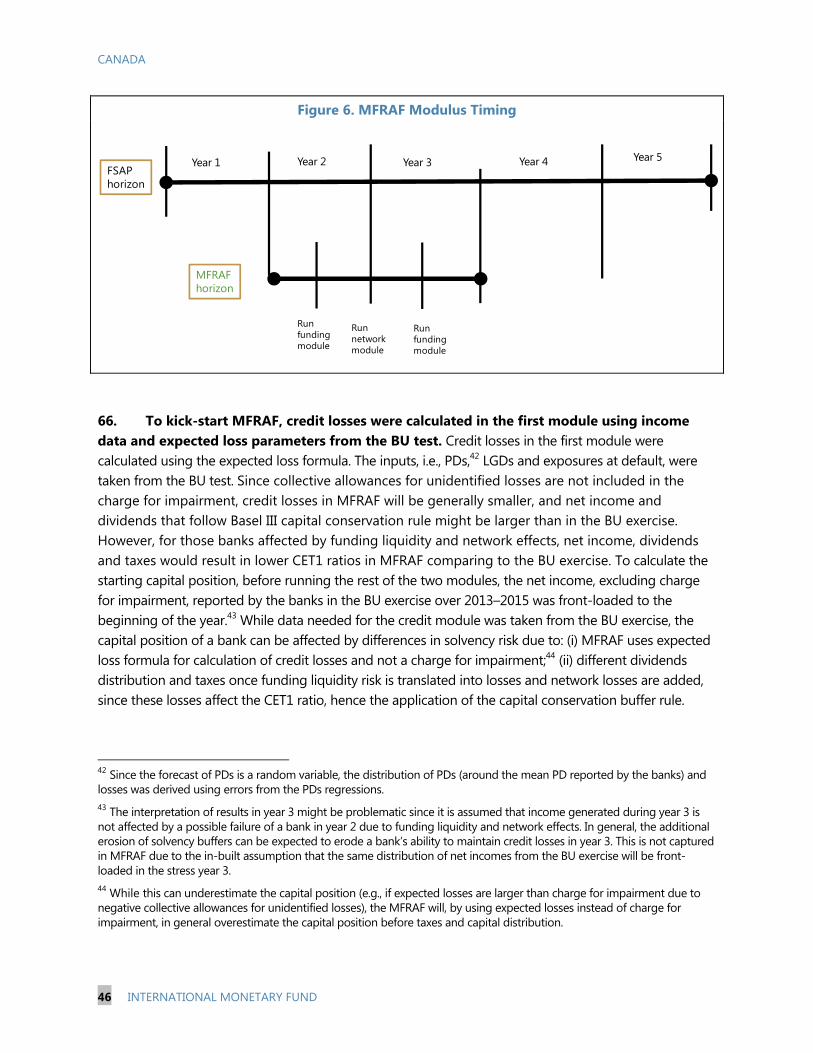
CANADA
46 INTERNATIONAL MONETARY FUND
MFRAFhorizon
FSAP horizon
Year 1 Year 2 Year 3 Year 4 Year 5
Run funding module
Run funding module
Run network module
Figure 6. MFRAF Modulus Timing
66. To kick-start MFRAF, credit losses were calculated in the first module using income data and expected loss parameters from the BU test. Credit losses in the first module were calculated using the expected loss formula. The inputs, i.e., PDs,42 LGDs and exposures at default, were taken from the BU test. Since collective allowances for unidentified losses are not included in the charge for impairment, credit losses in MFRAF will be generally smaller, and net income and dividends that follow Basel III capital conservation rule might be larger than in the BU exercise. However, for those banks affected by funding liquidity and network effects, net income, dividends and taxes would result in lower CET1 ratios in MFRAF comparing to the BU exercise. To calculate the starting capital position, before running the rest of the two modules, the net income, excluding charge for impairment, reported by the banks in the BU exercise over 2013–2015 was front-loaded to the beginning of the year.43 While data needed for the credit module was taken from the BU exercise, the capital position of a bank can be affected by differences in solvency risk due to: (i) MFRAF uses expected loss formula for calculation of credit losses and not a charge for impairment;44 (ii) different dividends distribution and taxes once funding liquidity risk is translated into losses and network losses are added, since these losses affect the CET1 ratio, hence the application of the capital conservation buffer rule.
42 Since the forecast of PDs is a random variable, the distribution of PDs (around the mean PD reported by the banks) and losses was derived using errors from the PDs regressions. 43 The interpretation of results in year 3 might be problematic since it is assumed that income generated during year 3 is not affected by a possible failure of a bank in year 2 due to funding liquidity and network effects. In general, the additional erosion of solvency buffers can be expected to erode a bank’s ability to maintain credit losses in year 3. This is not captured in MFRAF due to the in-built assumption that the same distribution of net incomes from the BU exercise will be front-loaded in the stress year 3. 44 While this can underestimate the capital position (e.g., if expected losses are larger than charge for impairment due to negative collective allowances for unidentified losses), the MFRAF will, by using expected losses instead of charge for impairment, in general overestimate the capital position before taxes and capital distribution.
CANADA
INTERNATIONAL MONETARY FUND 47
67. Funding liquidity was translated into losses in the second module. As initial credit losses of stress year 1 reduce the capital position of each bank and as under stressed market conditions the fire-sale discount affects the liquidity value of a bank’s assets that now might be insufficient to meet its maturing claims, a bank’s creditors form their view on the bank’s future solvency, which is assessed against the Canadian supervisory “all-in” threshold, and possibly decide not to roll over their claims. The capital ratio threshold used in the exercise was the supervisory CET1 ratio of 7 percent instead of the regulatory ratio since it is assumed that a bank would more likely face adverse reaction from its creditors if it breached the supervisory threshold rather than the regulatory one. Therefore, the severity of credit losses, the bank’s starting capital position, the asset-liability matching profile and the composition of the bank’s funding sources and liquidity value of assets may combine to give rise to funding liquidity risk.45 The liquidity profile of a bank was measured by the balance sheet liquidity (BSL) measure which is the ratio of the sum of liquid assets and illiquid assets multiplied by a fire sale discount to liabilities maturing over the next six months.46 It was assumed that if the BSL measure is above 100 percent there is no run on bank’s maturing liabilities. If the BSL measure is below 100 percent there is a positive probability that creditors choose to not roll over the bank’s obligations to them that mature within the next six months.47 Liquidity losses due to a run arise since a bank has to sell assets at a loss to cover maturing claims. These losses were assumed to be 2.25 percent of RWAs.48
68. The second module also took into account the risk that disruption in funding markets could also be the result of information contagion where a run would occur due to another bank defaulting. In MFRAF creditors will not only focus on the solvency and liquidity profile of the bank they are creditors of but also on other banks’ capital positions. When creditors observe another bank “defaulting” (i.e., CET1 ratio falling below 7 percent), they will update their beliefs on secondary market prices which are calibrated to be “low” or “high.”49 If this updating of creditors’ beliefs results in the fire-sale discount applied to illiquid assets lower than previously thought, the BSL measure is revised down which, combined with future solvency concerns, may lead creditors to decide not to roll over their claims.
45 More formally, the “run point” of losses is an increasing function of banks’ capital, liquid assets, the return on short-term debt, and a decreasing function of the amount of the net outflow, run-off rates applied to outflows and inflows, haircuts applied to liquid and illiquid assets and the opportunity cost of short-tem creditor. See Gauthier, He and Souissi (2010) for a more formal presentation of MFRAF. 46 Only the maturities that are deemed to be “risky” and affected in the liquidity stress scenario in a manner consistent with the LCR are taken into account. 47 This decision is modeled using the global games approach of Morris and Shin (2010), which is a coordination game with strategic complementarities between pay-offs from rolling over and the risk-free rate which they would receive if they do not roll over, and invest instead in a government security. 48 A sensitivity test was conducted where liquidity losses were assumed to be 1 percent of RWAs. Results show that the impact of liquidity risk in terms of CET1 ratio are noticeable, thus highlighting the importance of finding a meaningful way of calibrating this parameter. 49 In the liquidity calibration, the “good state” was referred as the state with high secondary market prices and the “bad state” as the state with low secondary market prices.

CANADA
48 INTERNATIONAL MONETARY FUND
69. Network effects due to defaults by counterparties were translated into losses in the third module. Spillover effects exist due to interbank exposures which give rise to counterparty credit losses. It was assumed that a bank that falls below the supervisory minimum will not be able to fulfill its obligations in the interbank markets, causing losses to its counterparties via an endogenous clearing mechanism and leading potentially to their default. These losses, together with losses due to materialization of funding liquidity and credit risks, had an additional impact on the capital position at the end of stress year 2. The network exercise was performed on the basis of exposures between banks that arise from deposits, traditional lending, reverse repos, bankers’ acceptances, cross-shareholdings, holdings of debt instruments, and OTC derivatives.
70. In the context of the FSAP, the BSL measure was calibrated to be broadly consistent with the LCR factors. The scenarios differed by different parameters of the BSL measure which is one of the key drivers of funding liquidity risk. The BSL was calculated based on data from the Net Cumulative Cash Flow (NCCF) liquidity measure50. For the purposes of the FSAP stress test, the BSL measure and its parameters were chosen to be consistent to the LCR. The calibration exercise of the BSL included: (i) BSL categories were matched to LCR items; for example, asset categories were mapped to be close to the HQLA definitions (i.e., levels 1, 2A and 2B); outflows categories were changed to get closer to LCR outflows definition; (ii) applied haircuts and run-off rates to most BSL categories correspond to the LCR calibration, (iii) all off-balance sheet items of the LCR (category D) were included in the BSL measure, (iv) derivatives related amounts were subtracted from liquid assets.
71. The BSL measure is different from the LCR measure. These differences are in part reflected specific features of Canadian banks and liquidity markets: (i) the set of HQLA was augmented by reverse repos and securities borrowed which carry zero haircuts in the baseline, (ii) it was assumed that banks can use illiquid assets to cover maturing liabilities i.e., illiquid assets (e.g., ABS) will not get 100% haircut as in the LCR exercise, (iii) the denominator, which represents liabilities for which banks’ creditors will decide whether to roll over or not, was calculated as all liabilities with a maturity date (cash outflows) falling within next 6 months plus a proportion of the each liability category that the LCR deems unstable,51 and (iv) the concept of tied securities and encumbrance of liquid assets is less strict than under the LCR definition. Moreover, while the LCR provides a measure of (funding) liquidity risk in the near-term, MFRAF translates this risk, via a parameterized model under behavioral assumptions, into a solvency impact. 50 The NCCF is OSFI’s internal liquidity, survival horizon metric that quantifies the length of time before an institution’s cumulative net cash flow turns negative, once factoring in the stock of available liquid assets. 51 According to the authorities, if the period considered was only 30 days, the losses would be limited and therefore, in most cases, the funding liquidity risk would not materialize. Moreover, maturities over a one-month period may vary from one month to the next; therefore, a 30-day period at a particular point of time is not representative of maturing liabilities. A 6-month period better captures the true dynamics of maturing liabilities. This difference in terms of the time horizon can explain the difference between the LCR and BSL numbers for banks that rely more on short-term funding (low LCR). While by using a 6-month period there will be less difference between banks in terms of funding, an advantage of the LCR is that it would identify banks which rely more on short-term funding and therefore are more prone to funding liquidity risk. At the same time, funding liquidity risk also depends on the composition of funding (e.g., secured versus unsecured, retail vs. wholesale); therefore, the time horizon considered is not the only factor to influence how prone banks are to funding liquidity risk.

CANADA
INTERNATIONAL MONETARY FUND 49
72. The framework was applied to the six largest banks using consolidated, supervisory data as of April 201352 under two scenarios against the supervisory capital threshold. A baseline and an adverse liquidity scenario were considered, using haircuts and run-off rates from the LCR (Table 12 and 13), but also taking into account specifics of Canadian liquidity markets. For both scenarios, for stress year 2, the NCCF data were used to get banks’ holdings of liquid and illiquid assets and maturing liabilities and calculate the BSL. For stress year 3, the three elements of BSL were updated based on proxies of those categories that banks reported for the BU exercise: (i) liquid assets were assumed to grow with the securities holdings, (ii) illiquid assets were assumed to grow with exposure at default, and (iii) maturing liabilities were assumed to grow in line with the interest-sensitive liabilities. These proxies from the BU exercise do not, however, take into account the impact of funding liquidity and network effects and may overestimate BSL in year 3. To calculate CET1 ratios, RWAs were taken from the BU exercise.53
Results 73. Bank liquidity stress tests suggest that, in aggregate, banks could withstand severe funding and market liquidity shocks. However, MFRAF results show that liquidity runs can lead to potentially large losses beyond solvency losses in the ToD or BU exercises, while network effects appear limited (Figure 7).
Year 2, liquidity module: In the baseline liquidity scenario, the marginal impact of liquidity risk is limited and suggests that in aggregate banks could withstand severe funding and market liquidity shocks. Only one bank is affected significantly by funding liquidity risk, generating losses equal to 200 basis point of “all-in” CET1. These losses, together with credit losses of 125 bps, would make this bank fall below the 4 percent regulatory threshold. The impact of funding liquidity for this bank is a consequence of the combination of the impact credit losses on its capital position before the liquidity risk has materialized, a mismatch in maturing liabilities and assets that can be sold in the distressed period and subsequent idiosyncratic run. The rest of the banks are marginally affected because of their high starting capital position and strong liquidity profiles . Information contagion did not materialize since only one bank experiences a run and because of the fact that all other banks have high liquidity ratios.
Year 2, network module: the bank that falls below the supervisory threshold in the liquidity module triggers network effects. This in turn generates deterioration in the capital position of the three banks which had largest interbank exposure to the bank that fell below the supervisory threshold. The marginal impact of the network effect on CET1 is rather small and ranges between 21 and 29 basis points because of interbank exposures which are small due to
52 Both domestic currency and foreign currency data were used. 53 By taking the RWAs from the BU test MFRAF results can be biased in either direction since selling illiquid, risky asset would imply lower RWAs, but selling liquid, safer assets would increase RWAs.
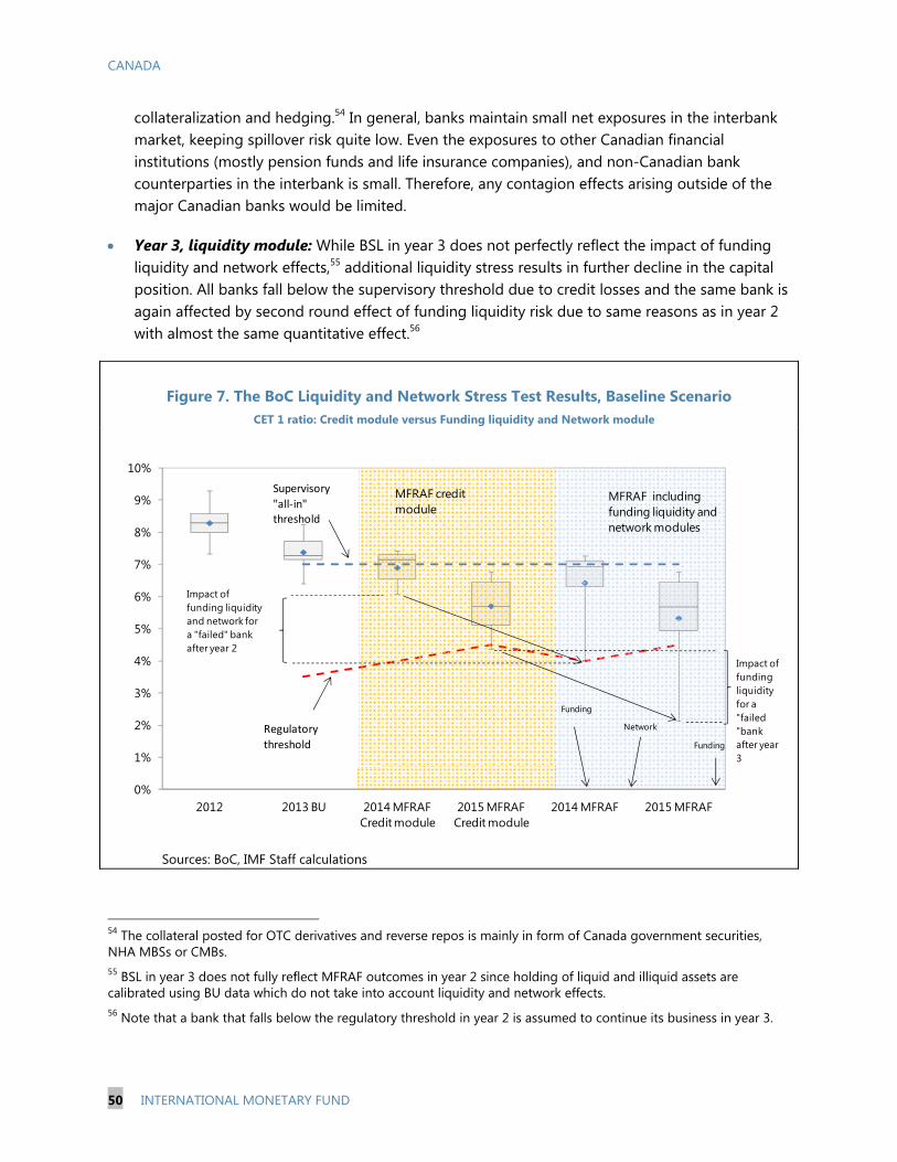
CANADA
50 INTERNATIONAL MONETARY FUND
0%
1%
2%
3%
4%
5%
6%
7%
8%
9%
10%
2012 2013 BU 2014 MFRAF Credit module
2015 MFRAF Credit module
2014 MFRAF 2015 MFRAF
Funding
Funding
Network
MFRAF including funding liquidity and network modules
Impact of funding liquidity and network for a "failed" bank after year 2
Impact of funding liquidity for a "failed "bank after year3
MFRAF creditmodule
Supervisory
"all-in" threshold
Regulatory
threshold
collateralization and hedging.54 In general, banks maintain small net exposures in the interbank market, keeping spillover risk quite low. Even the exposures to other Canadian financial institutions (mostly pension funds and life insurance companies), and non-Canadian bank counterparties in the interbank is small. Therefore, any contagion effects arising outside of the major Canadian banks would be limited.
Year 3, liquidity module: While BSL in year 3 does not perfectly reflect the impact of funding liquidity and network effects,55 additional liquidity stress results in further decline in the capital position. All banks fall below the supervisory threshold due to credit losses and the same bank is again affected by second round effect of funding liquidity risk due to same reasons as in year 2 with almost the same quantitative effect.56
Figure 7. The BoC Liquidity and Network Stress Test Results, Baseline Scenario
CET 1 ratio: Credit module versus Funding liquidity and Network module
Sources: BoC, IMF Staff calculations
54 The collateral posted for OTC derivatives and reverse repos is mainly in form of Canada government securities, NHA MBSs or CMBs. 55 BSL in year 3 does not fully reflect MFRAF outcomes in year 2 since holding of liquid and illiquid assets are calibrated using BU data which do not take into account liquidity and network effects. 56 Note that a bank that falls below the regulatory threshold in year 2 is assumed to continue its business in year 3.

CANADA
INTERNATIONAL MONETARY FUND 51
Figure8. Aggregate Loss Distributions, Baseline Scenario
End of stress year 2 End of stress year 3
Source: BoC
74. Adverse liquidity scenario results show that the marginal impact of liquidity risk would bring four banks below the regulatory threshold at the end of year 3 (Figure 9). Looking at the system-wide “all-in” CET1, cumulative credit losses of 215 bps over the two years relative to the base year) are augmented by cumulative losses equal to 235 bps due to materialization of funding liquidity risk and network effect that ensues due to severe market and funding distress57 in combination with low capital position in year 3.
Year 2, liquidity module: Even though the liquidity profiles of all banks are, only one bank —the same bank from the baseline scenario—is significantly affected by funding liquidity effects. This is because in year 2, the solvency position in year 2 is relatively strong; consequently, the combination of both is such that funding liquidity risk is limited. Again, contagion information effects are negligible since banks are already run upon for idiosyncratic reasons.
Year 2, network module: As in the baseline, the impact of network effects is benign due to small net interbank exposures.
57 This also includes network effects that materialize in stress year 2.

CANADA
52 INTERNATIONAL MONETARY FUND
Year 3, liquidity module: The combination of additional liquidity distress and decline in CET1 ratio due to credit losses generates additional sizeable liquidity losses which lead to four banks falling significantly below the regulatory threshold.
75. The MFRAF results show that there is sufficient capacity to provide official liquidity support even in the adverse scenario. MFRAF was used to determine how much official liquidity support should be provided if a particular liquidity distress event were to lead to the materialization of liquidity risk for banks, and so mitigate the related CET1 liquidity losses. The BoC analysis suggests that in the baseline scenario, the liquidity support would range between Can$5 billion and Can$9 billion, depending on market perception of prices of illiquid assets on secondary markets. In the adverse scenario, which is very extreme, it would range between Can$86 billion and Can$155 billion.58 This is in the range of liquidity support that the authorities provided during the 2008/2009 crisis.
76. The MFRAF results suggest that an effective framework for monitoring systemic risk requires considering banks’ capital, their funding profiles and spillover effects in a comprehensive manner (Figure 8 and 10). In general, failure to consider funding liquidity and spillover risks could underestimate the degree of systemic risk. This is particularly relevant for interconnected banking sectors where banks face big mismatches in their liquid assets and net outflows. In the BoC exercise, when funding liquidity risk and network effects are taken into account, banks face a further deterioration in their capital position relative to the results in the credit module of BU stress test that focuses on solvency risk only. MFRAF’s sequential framework allows decomposing the contributions of solvency risk, funding liquidity risk and network effects to the resulting CET1 ratio. Comparing the system-wide CET1 between the base year and stress year 3 in the credit module and liquidity and network module, the marginal impact of funding liquidity risk and network effects on capital position of the Big 6 over the two years is just around 35 basis points in the benchmark scenario but 235 basis points in the adverse scenario. Consequently, when liquidity risk and network effects are included, the distribution of losses shifts to the right. This means that a loss under funding liquidity and network module has a higher probability than a loss under the credit module i.e., if only solvency risk is taken into account (Figures 8 and 10). This is particularly true in the adverse scenario, where, for example, the probability of losses for the banking sector being 1 percent of RWAs is roughly zero percent, but increases to 15 percent when funding liquidity risk and network effects are included.
58 The higher the starting capital ratios of the banks, the lower would be the ex-post liquidity support required from the central bank.

CANADA
INTERNATIONAL MONETARY FUND 53
0%
1%
2%
3%
4%
5%
6%
7%
8%
9%
10%
2012 2013 BU 2014 MFRAF Credit module
2015 MFRAF Credit module
2014 MFRAF 2015 MFRAF
Funding
Funding
Network
MFRAF funding liquidity and network modules
Impact of funding liquidity and network for a "failed" bank after year 2
Impact of funding liquidity for a "failed "bank after year3
MFRAF creditmodule
Supervisory threshold
Regulatory threshold
Figure 9. The BoC Liquidity and Network Stress Test Results, Adverse Scenario CET 1 ratio Credit module versus Funding liquidity and Network module
Sources: BoC, IMF Staff calculations
Figure 10. Aggregate Loss Distributions, Adverse Scenario
End of stress year 2
Source: BoC

CANADA
54 INTERNATIONAL MONETARY FUND
Figure 10. Aggregate Loss Distributions, Adverse Scenario (Concluded)
End of stress year 3
Source: BoC
A. Recommendations and Policy Implications
77. While the authorities’ MFRAF is at the frontiers of systemic risk stress testing, the exercise has suggested that there is room for improvement. In particular:
Liquidity risk: OSFI should consider enhancing its own liquidity stress testing framework, which could strengthen its ability to regularly identify and monitor emerging liquidity risks. The LCR and NSFR metrics should be part of the stress testing framework.
Calibration of liquidity losses in MFRAF: Despite having an endogenous mechanism for liquidity runs, calibration of liquidity losses is done on an arbitrary basis. Finding a meaningful way of calibrating this parameter (e.g., by looking at mark-to-market losses during a downturn) would represent a major improvement of MFRAF.59
Balance Sheet Ratio dynamics: A run in Stress Year 3 which depends on the Balance Sheet Liquidity (BSL) ratio at the start of Stress Year 3 should be modeled in an internally consistent manner. Using the data for the BSL in Stress Year 3 from the BU exercise is inconsistent with the
59 However, the BoC argued that losses in the liquidity module of 2.25 of RWAs is a conservative estimate given that trading losses (realized and unrealized) during the 2008/2009 crisis were smaller than 2.25 of RWAs.

CANADA
INTERNATIONAL MONETARY FUND 55
results of the liquidity and network modules at the end of year 2, as the BU data do not reflect these effects. The BoC should try to incorporate these effects into the BSL metric.60
MFRAF future work: The BoC might want to embed MFRAF in a macroeconomic model that would allow them to simulate stress scenarios and calculate their impact within one framework while at the same time taking into account feedback loops between the financial system and the real economy. While it might be difficult to model individual banks’ behavior within a DSGE model, a general equilibrium model61 with a representative bank would at least provide a tool for validating the impact of funding liquidity risk “on average”. Alternately, the BoC might consider estimating a system of “ad-hoc” equations, which would represent a behavior of a particular sector of a small open economy. Modeling individual bank equations should be much easier than in a general equilibrium model. Within this system, feedback loops could be modeled using panel VAR for PDs and macroeconomic variables.
LIFE INSURANCE SECTOR—SOLVENCY STRESS TEST 78. The macro solvency stress test for life insurers follows assumptions comparable to the bank stress test, including the disorderly default of a European sovereign in the stressed scenario. Naturally, the relevance of financial market shocks is higher in an insurance stress test than in a bank stress test, so the adverse scenario included mainly variations of market variables such as lower equity prices, higher credit spreads and low interest rates. In addition, adverse rates of policyholders surrendering their life insurance policies were assumed.
79. The sample for the stress test included the three large life insurance companies Great West Life, Manulife and Sunlife, which account for a significant share of the Canadian Life & Health (L&H) market. In terms of assets, their market share amounts to 76 percent; in terms of premiums, more than 60 percent of the market is covered. Stresses were applied at the group level including international business which accounts for a substantial part of the three big companies, mainly via operations in the United States, as well as in Asia and Europe.
80. As a valuation framework for the stress test, the Canadian valuation regime being in place on 1 January 2013 was used. Capital projections were made in accordance with OSFI guidelines on the Minimum Continuing Capital and Surplus Requirement (MCCSR). Companies were instructed not to make use of extraordinary management actions like capital increases or discontinuation of business lines.
81. The three large life insurance companies show quite robust results in the stress test. In the baseline scenario, which was characterized by gradually increasing interest rates, rising equity
60 The same applies to the calculation of RWAs. 61 A la Iacoviello (2005), Christensen and Meh (2011) and Christensen, Corrigan, Mendicino and Nishiyama (2009) for the real economy part and Gerali, Neri, Sassa and Signoretti (2010) for the financial side of the model, where liquidity markets should be additionally modeled.
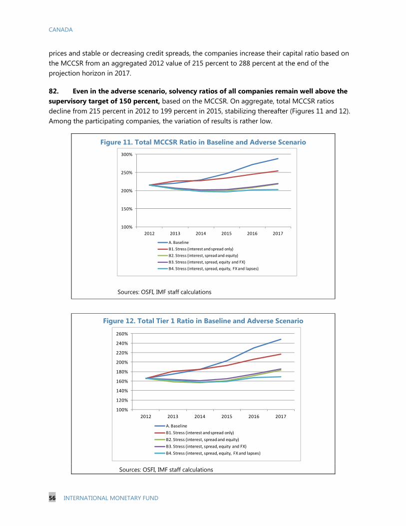
CANADA
56 INTERNATIONAL MONETARY FUND
prices and stable or decreasing credit spreads, the companies increase their capital ratio based on the MCCSR from an aggregated 2012 value of 215 percent to 288 percent at the end of the projection horizon in 2017.
82. Even in the adverse scenario, solvency ratios of all companies remain well above the supervisory target of 150 percent, based on the MCCSR. On aggregate, total MCCSR ratios decline from 215 percent in 2012 to 199 percent in 2015, stabilizing thereafter (Figures 11 and 12). Among the participating companies, the variation of results is rather low.
Figure 11. Total MCCSR Ratio in Baseline and Adverse Scenario
Sources: OSFI, IMF staff calculations
Figure 12. Total Tier 1 Ratio in Baseline and Adverse Scenario
Sources: OSFI, IMF staff calculations
100%
150%
200%
250%
300%
2012 2013 2014 2015 2016 2017
A. Baseline
B1. Stress (interest and spread only)
B2. Stress (interest, spread and equity)
B3. Stress (interest, spread, equity and FX)
B4. Stress (interest, spread, equity, FX and lapses)
100%
120%
140%
160%
180%
200%
220%
240%
260%
2012 2013 2014 2015 2016 2017
A. Baseline
B1. Stress (interest and spread only)
B2. Stress (interest, spread and equity)
B3. Stress (interest, spread, equity and FX)
B4. Stress (interest, spread, equity, FX and lapses)

CANADA
INTERNATIONAL MONETARY FUND 57
83. Net income remains positive under the adverse scenario in each year of the projection horizon and is expected to recover quickly from its lows in 2013 (Figure 13). On aggregate, net income declines by 20 percent in 2013 and rises in each year thereafter. At the end of the projection horizon in 2017, net income is 15 percent higher than in 2012. In the baseline scenario, net income is expected to double within five years.
Figure 13. Net Income in Baseline and Adverse Scenario in million Can$
Sources: OSFI, IMF staff calculation
84. In the first year of the projection horizon, share price declines and adverse policyholders’ lapse rates add most to the overall impact on insurers’ capital and net income under the adverse scenario (Figure 14). Less pronounced is the effect of lower risk-free interest rates in the first year of the projection horizon, as companies have already built up substantial reserves in recent years. Starting in 2014, however, interest rate and credit spread developments contribute most to the deterioration of solvency rates vis-à-vis the baseline scenario. Exchange rate movements included in the adverse scenario, such as a 10 percent depreciation of the Canadian dollar versus the U.S. dollar, have a negligible effect on solvency ratios and net income given the close currency matching of assets and liabilities.
0
2,000
4,000
6,000
8,000
10,000
12,000
2012 2013 2014 2015 2016 2017
Baseline
Stress (interest, spread, equity, FX and lapses)
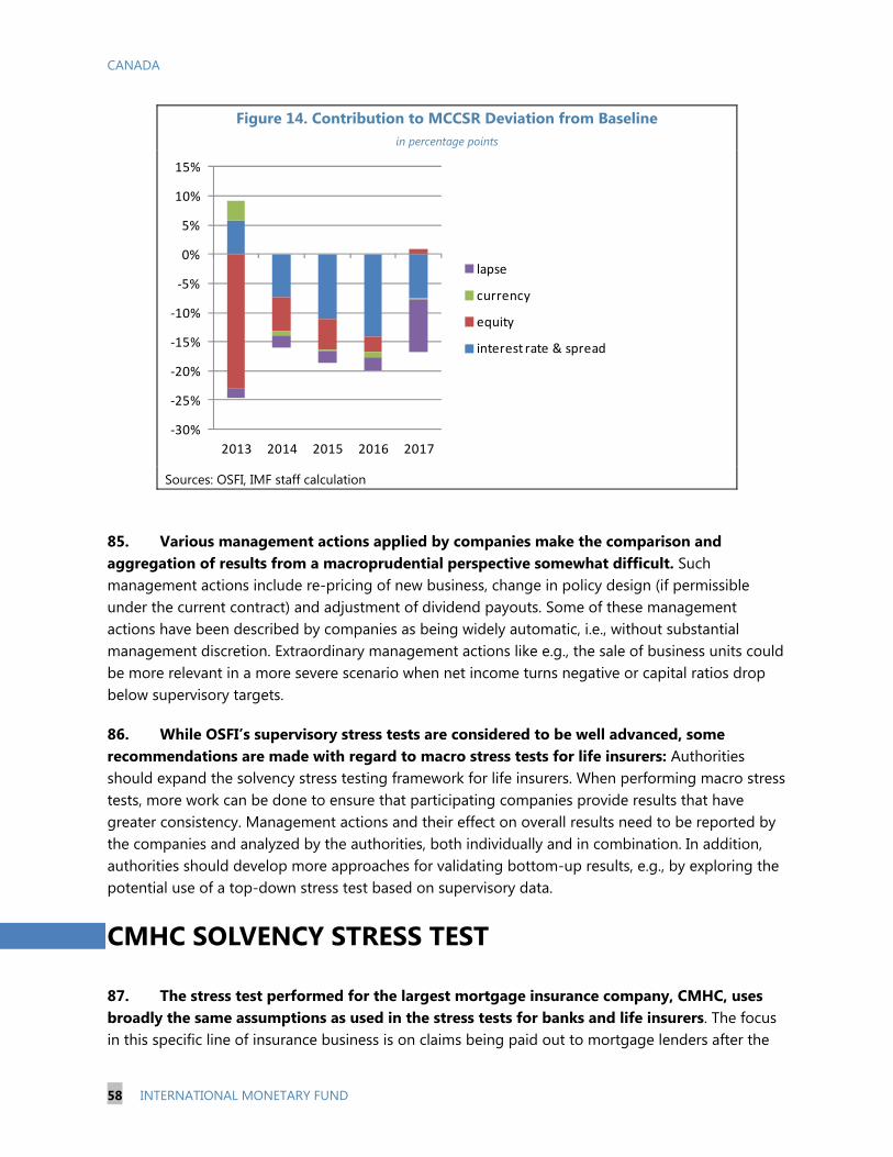
CANADA
58 INTERNATIONAL MONETARY FUND
Figure 14. Contribution to MCCSR Deviation from Baseline in percentage points
Sources: OSFI, IMF staff calculation
85. Various management actions applied by companies make the comparison and aggregation of results from a macroprudential perspective somewhat difficult. Such management actions include re-pricing of new business, change in policy design (if permissible under the current contract) and adjustment of dividend payouts. Some of these management actions have been described by companies as being widely automatic, i.e., without substantial management discretion. Extraordinary management actions like e.g., the sale of business units could be more relevant in a more severe scenario when net income turns negative or capital ratios drop below supervisory targets.
86. While OSFI’s supervisory stress tests are considered to be well advanced, some recommendations are made with regard to macro stress tests for life insurers: Authorities should expand the solvency stress testing framework for life insurers. When performing macro stress tests, more work can be done to ensure that participating companies provide results that have greater consistency. Management actions and their effect on overall results need to be reported by the companies and analyzed by the authorities, both individually and in combination. In addition, authorities should develop more approaches for validating bottom-up results, e.g., by exploring the potential use of a top-down stress test based on supervisory data.
CMHC SOLVENCY STRESS TEST 87. The stress test performed for the largest mortgage insurance company, CMHC, uses broadly the same assumptions as used in the stress tests for banks and life insurers. The focus in this specific line of insurance business is on claims being paid out to mortgage lenders after the
-30%
-25%
-20%
-15%
-10%
-5%
0%
5%
10%
15%
2013 2014 2015 2016 2017
lapse
currency
equity
interest rate & spread
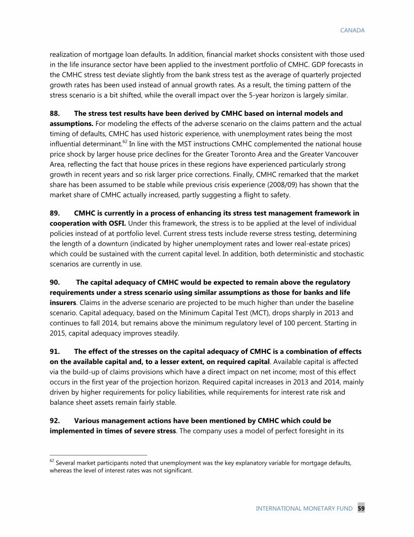
CANADA
INTERNATIONAL MONETARY FUND 59
realization of mortgage loan defaults. In addition, financial market shocks consistent with those used in the life insurance sector have been applied to the investment portfolio of CMHC. GDP forecasts in the CMHC stress test deviate slightly from the bank stress test as the average of quarterly projected growth rates has been used instead of annual growth rates. As a result, the timing pattern of the stress scenario is a bit shifted, while the overall impact over the 5-year horizon is largely similar.
88. The stress test results have been derived by CMHC based on internal models and assumptions. For modeling the effects of the adverse scenario on the claims pattern and the actual timing of defaults, CMHC has used historic experience, with unemployment rates being the most influential determinant.62 In line with the MST instructions CMHC complemented the national house price shock by larger house price declines for the Greater Toronto Area and the Greater Vancouver Area, reflecting the fact that house prices in these regions have experienced particularly strong growth in recent years and so risk larger price corrections. Finally, CMHC remarked that the market share has been assumed to be stable while previous crisis experience (2008/09) has shown that the market share of CMHC actually increased, partly suggesting a flight to safety.
89. CMHC is currently in a process of enhancing its stress test management framework in cooperation with OSFI. Under this framework, the stress is to be applied at the level of individual policies instead of at portfolio level. Current stress tests include reverse stress testing, determining the length of a downturn (indicated by higher unemployment rates and lower real-estate prices) which could be sustained with the current capital level. In addition, both deterministic and stochastic scenarios are currently in use.
90. The capital adequacy of CMHC would be expected to remain above the regulatory requirements under a stress scenario using similar assumptions as those for banks and life insurers. Claims in the adverse scenario are projected to be much higher than under the baseline scenario. Capital adequacy, based on the Minimum Capital Test (MCT), drops sharply in 2013 and continues to fall 2014, but remains above the minimum regulatory level of 100 percent. Starting in 2015, capital adequacy improves steadily.
91. The effect of the stresses on the capital adequacy of CMHC is a combination of effects on the available capital and, to a lesser extent, on required capital. Available capital is affected via the build-up of claims provisions which have a direct impact on net income; most of this effect occurs in the first year of the projection horizon. Required capital increases in 2013 and 2014, mainly driven by higher requirements for policy liabilities, while requirements for interest rate risk and balance sheet assets remain fairly stable.
92. Various management actions have been mentioned by CMHC which could be implemented in times of severe stress. The company uses a model of perfect foresight in its
62 Several market participants noted that unemployment was the key explanatory variable for mortgage defaults, whereas the level of interest rates was not significant.
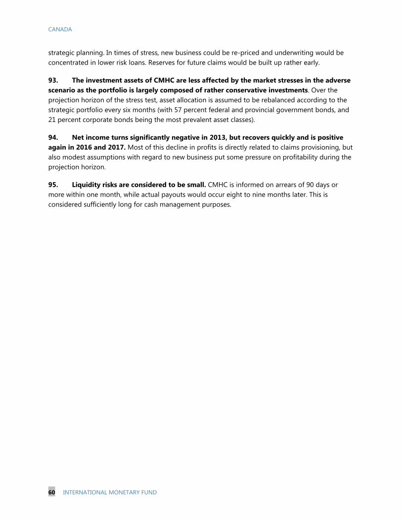
CANADA
60 INTERNATIONAL MONETARY FUND
strategic planning. In times of stress, new business could be re-priced and underwriting would be concentrated in lower risk loans. Reserves for future claims would be built up rather early.
93. The investment assets of CMHC are less affected by the market stresses in the adverse scenario as the portfolio is largely composed of rather conservative investments. Over the projection horizon of the stress test, asset allocation is assumed to be rebalanced according to the strategic portfolio every six months (with 57 percent federal and provincial government bonds, and 21 percent corporate bonds being the most prevalent asset classes).
94. Net income turns significantly negative in 2013, but recovers quickly and is positive again in 2016 and 2017. Most of this decline in profits is directly related to claims provisioning, but also modest assumptions with regard to new business put some pressure on profitability during the projection horizon.
95. Liquidity risks are considered to be small. CMHC is informed on arrears of 90 days or more within one month, while actual payouts would occur eight to nine months later. This is considered sufficiently long for cash management purposes.

CANADA
INTERNATIONAL MONETARY FUND 61
Banks- Total Big 6Other domestic
banksForeign
subsidiariesForeign
branchesBasic dataTotal assets, in billions of CAD 3,721,258 3,400,987 128,375 124,125 67,771 In percent of GDP 204.7 187.1 7.1 6.8 3.7Nominal GDP 1,817,604.0
Financial Soundness indicators
Capital adequacy, in percentTotal capital ratio 16.1 15.8 16.8 21.1Tier 1 ratio 13.4 13.0 13.5 19.1Core tier 1 ratio (Apr 2013, transitional basis) 12.4 12.3 13.3 17.2Capital to assets 5.5 5.4 5.4 11.1
Credit risk, in percentNPLs net of specific provisions to capital 5.6 5.8 2.6 4.1NPLs net of specific and general provisions to capital 0.7 1.0 -2.0 1.1NPLs to gross loans 0.6 0.7 0.2 1.2 0.2Provisions (specific) to NPL 22.4 21.6 27.3 33.1 29.8Provisions (specific and general) to NPL 90.4 86.5 154.3 81.6 773.4Distribution of loans by currencyDomestic currency 61.1 58.6 98.8 85.2 73.2Foreign currency 38.9 41.4 1.2 14.8 26.8
Profitability, in percentReturn on assets (net income/end period assets) 0.8 0.9 0.5 0.8 -0.2Return on equity (net income/end period shareholder's equity excluding preffered shares)
22.7 23.9 13.8 11.8
Interest margin on gross income 39.9 39.5 45.0 40.2 53.0Trading income to gross income 3.5 3.6 1.0 4.3 1.1Non-interest Expenses to Gross Income 42.7 42.3 36.2 42.0 71.1Liquidity, in percentLiquid assets to total assets 12.4Liquid assets to short-term liabilities 44.9Customer deposits to loans 44.1 43.5 73.1 41.4 0.5FX and derivative risk, in percentNet open FX position to equity 20.6 18.9 8.1 2.6FX loans to total loans 26.9 29.0 0.2 8.9 19.5FX liabilities to total liabilities 40.1 42.5 1.7 15.0 36.4
Appendix I. Statistical Annex
Table 10. FSIs: Big 6 versus the Rest of the Banking System
Sources: OSFI, IMF, Financial Soundness Indicators (FSI) database, IMF Staff calculations

CANADA
62 INTERNATIONAL MONETARY FUND
0
200
400
600
800
1,000
1,200
1,400
Consumer credit 1/ Residential mortgage credit
Short-term business credit
Non-residential mortgages
Other business credit
Other Equity & WarrantsBonds & Debentures Bankers' acceptancesSecuritization by banks & non-banks Credit unions & caisses populaires Chartered banks
Household and Business Credit(Billions of CAD$)
71%
44% 67%
57%49%
31% 47%
0% 17%
27%
14%
11%12%
16%
13% 10%
22% 18%
22% 13%24%
25%19%
32%
10%8% 3%
1%
2% 15%
0
1,000
2,000
3,000
4,000
5,000
6,000
7,000
8,000
RBC TD 2/ BNS 3/ BMO 4/ CIBC 5/ NBC 6/ Desjardins 7/
Personal & Commercial BankingPersonal & Commercial: CanadaPersonal & Commercial: U.S. and other
Wealth ManagementCapital MarketsInsurance
Net Income by Business Segment, FY 2012, Millions of Canadian dollars
Figure 15. Developments in Banking Sector
Credit intermediation in Canada is dominated by
chartered banks.
The largest banks have diversified business models,
covering all the main business segments, as well as the
range of geographic and business sectors in Canada.
Canadian banks’ assets are well-diversified, and their composition has remained remarkably stable in recent years, with the
exception of insured mortgages which increased due to introduction of the IFRS at the end of 2011.
Sources: Haver, BoC, OSFI, financial institutions’
annual reports, IMF staff calculations
Storyline goes here….
6%10%
6%
7%
10%
18%
7%3%
10%
8%
6%
9%
6%
11%
9%
6%
11%
12%9%
2%
8%
10%
8%
8%
Cash&deposits6%
Private debt9%
Shares6%
Governement securities
6%
Consumer loans 13%
Business loans11%
Repos9%
Other loans2%
Insured mortgages
14%
Uninsured mortgages
10%
Derivatives7%
Other7%
2000M12
2007M12
2012M12
Assets(Percent of total assets)
28%
29%10%
0%6%
4%
7%
4%2%
5% 5%25%
34%
7%
0%
8%
6%
7%
2%1%
6%4%
Individual deposits27%
Other deposits32%
Deposit-taking institutions
3%
Governement deposits
1%
Derivatives7%
Obligations related to borrowed securities
4%
Obligations related to assets sold under repo
7%
Acceptances1%
Subordinated debt1%
Mortgages and loans payable
6%
Other5%
Shareholders equity
6%
2012M12
2007M12
2000M12
Liabilities(Percent of total liabilities)

CANADA
INTERNATIONAL MONETARY FUND 63
Big-6 banks Other banks0%
20%
40%
60%
80%
100%Other
Derivatives
Uninsured mortgages
Insured mortgages
Other loans
Repos
Business loans
Consumer loans
Non-mortgage Loans
Governement securities
Shares
Private debt
Cash&deposits
Assets
Big-6 banks Other banks0%
20%
40%
60%
80%
100%Shareholders equity
Other
Mortgages&loans
Subordinated debt
Acceptances
Repos
Borrowed securities
Derivatives
Governement deposits
Deposit-taking institutions
Other deposits
Individual deposits
Liabilities
Developments in Banking Sector, continued
Bank funding is dominated by individual and other deposits, with total deposits amounting to about two-thirds of banks’
balance sheets.
Source: OSFI

CANADA
64 INTERNATIONAL MONETARY FUND
(10,000)
(5,000)
-
5,000
10,000
15,000
20,000
25,000
30,000
35,000
2008 2009 2010 2011 2012
Other /1 /2
Central and South America
Caribbean
US
Canada
78%
44%
64%
14%
30%
25%
7%
30%
11%
0%
10%
20%
30%
40%
50%
60%
70%
80%
90%
100%
Credit exposure Impaired loans Impairment losses
Other
US
Canada
80%
66%54%
70% 83%99%
11%
7%
8%24%
1%
1%
9%
26%38%
7%
15%
0
1,000
2,000
3,000
4,000
5,000
6,000
7,000
8,000
RBC TD BNS 2/ BMO CIBC 3/ NBC
CanadaU.S.Other
Net Income by Geography, FY 2012, Millions of Canadian dollars)
0
10
20
30
40
50
60
70
Dec-05 Dec-07 Dec-10 Dec-12
Canadian Banks Consolidated Foreign Claims (Percent of total foreign claims)
Developments in Banking Sector, continued
Canadian banks’ foreign operations have increased over
time, notably in the U.S.
Regional exposure is concentrated towards the United
States, Latin America and the Caribbean.
Over the last five years, income volatility has been highest
for U.S. operations.
The relative share of impaired loans and impairment
losses is higher in the U.S. and other foreign markets than
in Canada.
Source: BoC, OSFI, banks’ annual reports, IMF Staff
calculations
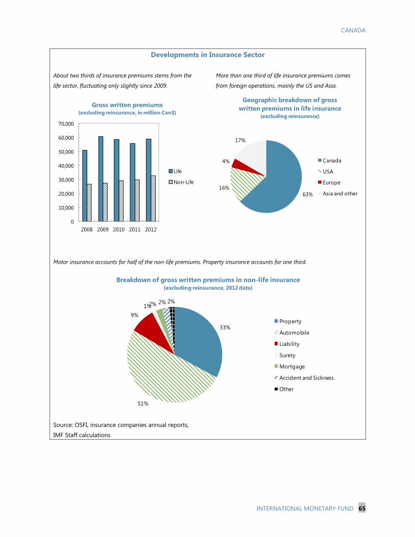
CANADA
INTERNATIONAL MONETARY FUND 65
Developments in Insurance Sector
About two thirds of insurance premiums stems from the
life sector, fluctuating only slightly since 2009.
More than one third of life insurance premiums comes
from foreign operations, mainly the US and Asia.
Motor insurance accounts for half of the non-life premiums. Property insurance accounts for one third.
Source: OSFI, insurance companies annual reports,
IMF Staff calculations
0
10,000
20,000
30,000
40,000
50,000
60,000
70,000
2008 2009 2010 2011 2012
Gross written premiums(excluding reinsurance, in million Can$)
Life
Non-Life
63%16%
4%
17%
Geographic breakdown of gross written premiums in life insurance
(excluding reinsurance)
Canada
USA
Europe
Asia and other
33%
51%
9%1%2% 2% 2%
Breakdown of gross written premiums in non-life insurance(excluding reinsurance, 2012 data)
Property
Automobile
Liability
Surety
Mortgage
Accident and Sickness
Other

CANADA
66 INTERNATIONAL MONETARY FUND
Developments in Insurance Sector, continued
In terms of assets, the life insurance sector is ten times
larger than the non-life sector; in addition it has grown
faster since 2008.
Solvency ratios in the life insurance sector were relatively
stable since 2008 and constantly above 200 percent.
Segregated accounts make up a large part of life insurers’ assets. Apart from these, bonds and debentures are the most
important asset class by a wide margin while investments in shares and property are relatively small.
Source: OSFI, life insurance companies annual reports,
IMF Staff calculations
0
200,000
400,000
600,000
800,000
1,000,000
1,200,000
2008 2009 2010 2011 2012
Insurance sector assets(in million Can$)
Life
Non-Life
0
50
100
150
200
250
2008 2009 2010 2011 2012
Solvency ratios(life insurance, in percent)
MCCSR ratio - Total
MCCSR ratio - Tier 1
2%
31%
7%
3%2%
40%
4%
8%3%
Asset allocation of life insurers(2012 data)
Cash and Cash Equivalents
Bonds and Debentures
Mortgage Loans
Common Shares
Investment Properties
Segregated Funds Net Assets
Reinsurance Assets
Other investment assets
Other assets
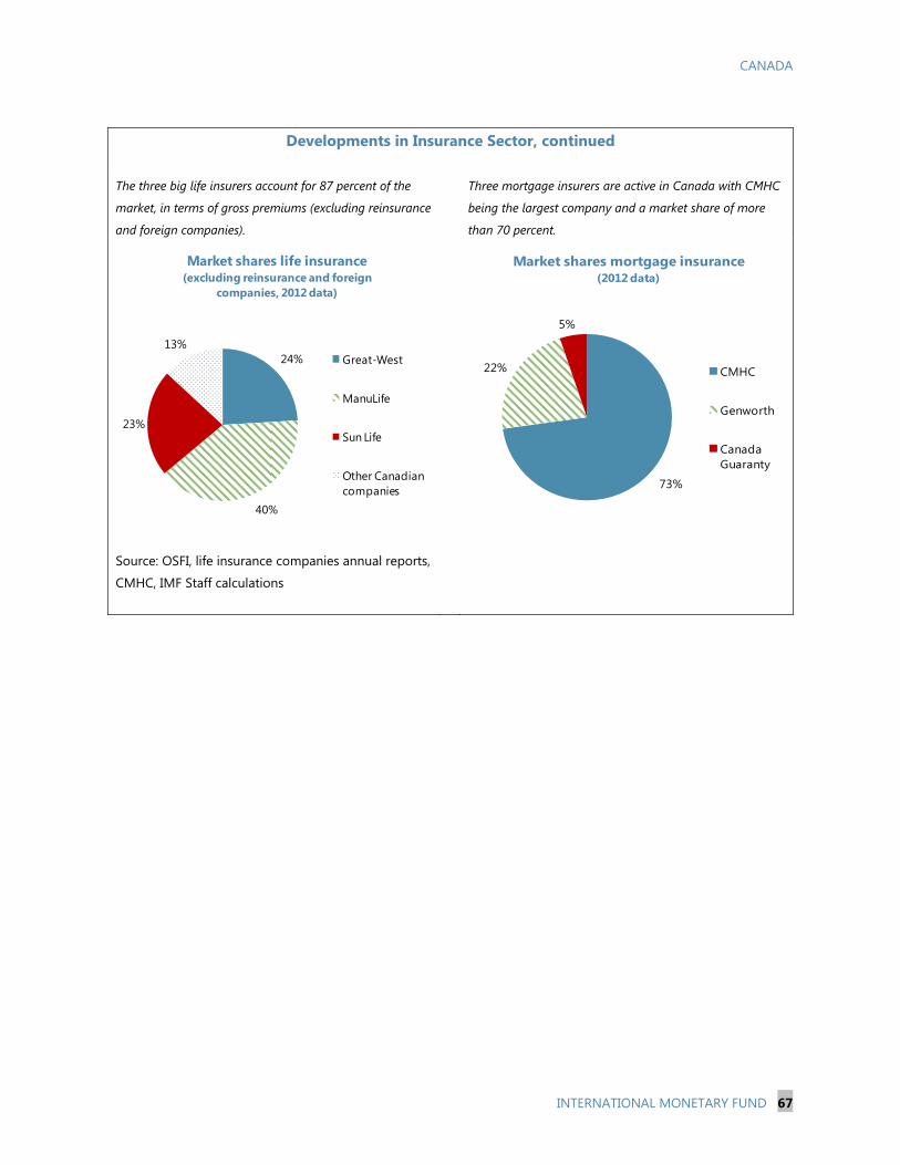
CANADA
INTERNATIONAL MONETARY FUND 67
Developments in Insurance Sector, continued
The three big life insurers account for 87 percent of the
market, in terms of gross premiums (excluding reinsurance
and foreign companies).
Three mortgage insurers are active in Canada with CMHC
being the largest company and a market share of more
than 70 percent.
Source: OSFI, life insurance companies annual reports,
CMHC, IMF Staff calculations
24%
40%
23%
13%
Market shares life insurance(excluding reinsurance and foreign
companies, 2012 data)
Great-West
ManuLife
Sun Life
Other Canadian companies 73%
22%
5%
Market shares mortgage insurance(2012 data)
CMHC
Genworth
Canada Guaranty

CANADA
68 INTERNATIONAL MONETARY FUND
IMF top down OSFI top down Bottom up
Number of banks falling below supervisory threshold (year) 6 (2015) 5 (2015) 5 (2015) regulatory threshold (year) 4 (2016) 2 (2017) 1 (2017)
Recapitalization needs (supervisory threshold) % 2012 gross income 30% 20% 9% % 2012 net income 150% 90% 40% % nominal GDP 2.5% 1.5% 0.7%
Recapitalization needs (regulatory threshold) % 2012 gross income 7% 3% 0.4% % 2012 net income 30% 15% 2% % nominal GDP 0.5% 0.2% 0%
Baseline Adverse
Number of banks falling below regulatory threshold year 1 1 1 year 2 1 4
Cummulative impact (year 2 & 3) on system-wide CET1 solvency risk 215 bps 215 bps funding liquidty and network efects 35 bps 235 bps
Liquidity needs (estimated by the BoC) $5-$9 bn in each year $90-$160 bn in each year
Table 11. Summary of Banks’ Stress Testing Results
Solvency stress test
Liquidity stress test- MFRAF, individual and network effects
Source: BoC, OSFI, IMF Staff calculations

CANADA
INTERNATIONAL MONETARY FUND 69
-4.0
-2.0
0.0
2.0
4.0
6.0
2000 2002 2004 2006 2008 2010 2012 2014 2016
Stress scenario Baseline scenario
0.0
2.0
4.0
6.0
8.0
10.0
12.0
14.0
2000 2002 2004 2006 2008 2010 2012 2014 2016
Stress scenario Baseline scenario
-25-20-15-10-505
1015
2000 2002 2004 2006 2008 2010 2012 2014 2016
Stress scenario Baseline scenario
-30
-20
-10
0
10
20
30
2000 2002 2004 2006 2008 2010 2012 2014 2016
Stress scenario Baseline scenario
0.5
0.6
0.7
0.8
0.9
1.0
1.1
1.2
2000 2002 2004 2006 2008 2010 2012 2014 2016
Stress scenario Baseline scenario
0.0
1.0
2.0
3.0
4.0
5.0
6.0
7.0
2000 2002 2004 2006 2008 2010 2012 2014 2016
Stress scenario Baseline scenario
Figure 16. Scenarios—Canada, Main Variables
GDP growth Unemployment rate
House prices (CREA) growth Equity price (TSX) growth
CAD/USD exchange rate BoC target interest rate
Source: BoC, OSFI, Haver, IMF Staff calculations

CANADA
70 INTERNATIONAL MONETARY FUND
-4.0-3.0-2.0-1.00.01.02.03.04.05.0
2000 2002 2004 2006 2008 2010 2012 2014 2016
Stress scenario Baseline scenario
0.0
2.0
4.0
6.0
8.0
10.0
12.0
14.0
2000 2002 2004 2006 2008 2010 2012 2014 2016
Stress scenario Baseline scenario
-6.0
-4.0
-2.0
0.0
2.0
4.0
6.0
2000 2002 2004 2006 2008 2010 2012 2014 2016
Stress scenario Baseline scenario
0.0
5.0
10.0
15.0
20.0
2000 2002 2004 2006 2008 2010 2012 2014 2016
Stress scenario Baseline scenario
0.0
20.0
40.0
60.0
80.0
100.0
200020022004200620082010201220142016
Stress scenario Baseline scenario
Figure 17. Scenarios—US, Euro Area, Other, Main Variables
U.S. GDP growth U.S. unemployment rate
Euro area GDP growth Euro area unemployment rate
Oil price (West Texas International)
Source: BoC, OSFI, Haver, IMF Staff calculations
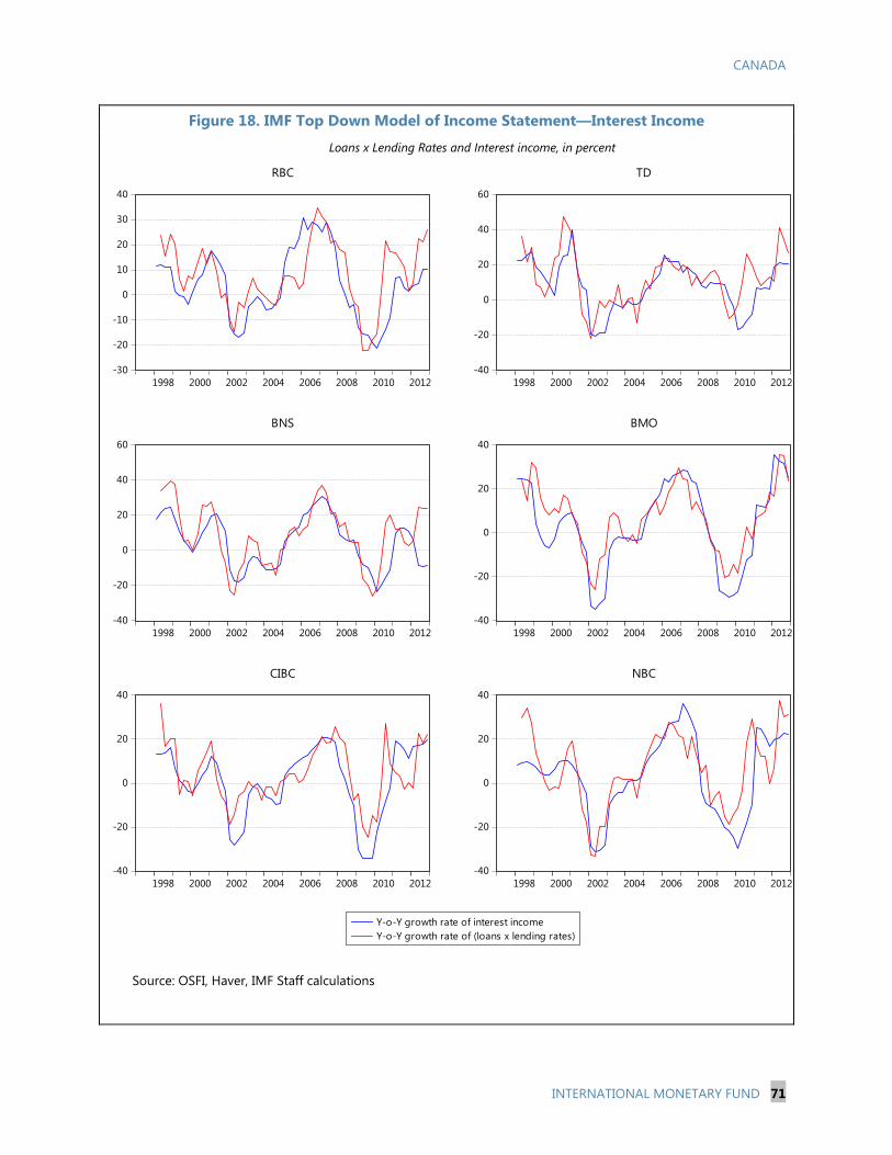
CANADA
INTERNATIONAL MONETARY FUND 71
-30
-20
-10
0
10
20
30
40
1998 2000 2002 2004 2006 2008 2010 2012
RBC
-40
-20
0
20
40
60
1998 2000 2002 2004 2006 2008 2010 2012
TD
-40
-20
0
20
40
60
1998 2000 2002 2004 2006 2008 2010 2012
BNS
-40
-20
0
20
40
1998 2000 2002 2004 2006 2008 2010 2012
BMO
-40
-20
0
20
40
1998 2000 2002 2004 2006 2008 2010 2012
CIBC
-40
-20
0
20
40
1998 2000 2002 2004 2006 2008 2010 2012
Y-o-Y growth rate of interest incomeY-o-Y growth rate of (loans x lending rates)
NBC
Figure 18. IMF Top Down Model of Income Statement—Interest Income
Loans x Lending Rates and Interest income, in percent
Source: OSFI, Haver, IMF Staff calculations

CANADA
72 INTERNATIONAL MONETARY FUND
-80
-40
0
40
80
1998 2000 2002 2004 2006 2008 2010 2012
RBC
-60
-40
-20
0
20
40
60
1998 2000 2002 2004 2006 2008 2010 2012
TD
-80
-40
0
40
80
120
1998 2000 2002 2004 2006 2008 2010 2012
BNS
-80
-40
0
40
80
1998 2000 2002 2004 2006 2008 2010 2012
BMO
-60
-40
-20
0
20
40
60
1998 2000 2002 2004 2006 2008 2010 2012
CIBC
-80
-40
0
40
80
1998 2000 2002 2004 2006 2008 2010 2012
Y-o-Y growth rate of interest expenseY-o-Y growth rate of (deposits x deposit rates)
NBC
Figure 19. IMF Top Down Model of Income Statement—Interest Expense
Deposits x Interest Rates and Interest expense, in percent
Source: OSFI, Haver, IMF Staff calculations

CANADA
INTERNATIONAL MONETARY FUND 73
-6
-4
-2
0
2
4
6
1998 2000 2002 2004 2006 2008 2010 2012
RBC
-4
-2
0
2
4
1998 2000 2002 2004 2006 2008 2010 2012
TD
-6
-4
-2
0
2
4
6
1998 2000 2002 2004 2006 2008 2010 2012
BNS
-4
-3
-2
-1
0
1
2
3
1998 2000 2002 2004 2006 2008 2010 2012
BMO
-6
-4
-2
0
2
4
1998 2000 2002 2004 2006 2008 2010 2012
CIBC
-4
-3
-2
-1
0
1
2
3
1998 2000 2002 2004 2006 2008 2010 2012
Y-o-Y change in trading incomeY-o-Y change in TSXY-o-Y change in nominal income
NBC
Figure 20. IMF Top Down Model of Income Statement—Trading Income
Trading income, Nominal GDP, TSX, standardized data

CANADA
74 INTERNATIONAL MONETARY FUND
.010
.015
.020
.025
.030
.035
.040
97 98 99 00 01 02 03 04 05 06 07 08 09 10 11 12
RBC TD BNSBMO CIBC NBC
.000
.001
.002
.003
.004
.005
.006
.007
.008
97 98 99 00 01 02 03 04 05 06 07 08 09 10 11 12
RBC TD BNSBMO CIBC NBC
Figure 21. IMF Top Down Model of Income Statement—Non-interest Income
Non-interest income in proportion of nominal GDP
Sources: OSFI, Haver, IMF Staff calculations
Figure 22. IMF Top Down Model of Income Statement—Non-interest Expense Non-interest expense in proportion of balance sheet
Sources: OSFI, Haver, IMF Staff calculations

CANADA
INTERNATIONAL MONETARY FUND 75
-10
0
10
20
30
40
1998 2000 2002 2004 2006 2008 2010 2012
RBC
-10
0
10
20
30
40
50
1998 2000 2002 2004 2006 2008 2010 2012
TD
-10
0
10
20
30
1998 2000 2002 2004 2006 2008 2010 2012
BNS
-20
-10
0
10
20
30
40
1998 2000 2002 2004 2006 2008 2010 2012
BMO
-20
-10
0
10
20
30
1998 2000 2002 2004 2006 2008 2010 2012
CIBC
-20
-10
0
10
20
30
40
1998 2000 2002 2004 2006 2008 2010 2012
Y-o-Y growth rate of loansY-o-Y growth rate of deposits
NBC
Figure 23. IMF Top Down Assumptions—Loans, Deposits
Loan and deposits, in percent63
Sources: OSFI, IMF Staff calculations
63 Growth rate of loans is 2012 is much higher than the growth rate of deposits due to IFRS implementation in 2011 Q4.

CANADA
76 INTERNATIONAL MONETARY FUND
-10
0
10
20
30
1998 2000 2002 2004 2006 2008 2010 2012
RBC
-10
0
10
20
30
40
1998 2000 2002 2004 2006 2008 2010 2012
TD
-10
0
10
20
30
1998 2000 2002 2004 2006 2008 2010 2012
BNS
-8
-4
0
4
8
12
16
20
24
1998 2000 2002 2004 2006 2008 2010 2012
BMO
-20
-10
0
10
20
30
1998 2000 2002 2004 2006 2008 2010 2012
CIBC
-10
0
10
20
30
40
1998 2000 2002 2004 2006 2008 2010 2012
Y-o-Y growht rate of loansY-o-Y growht rate of balance sheet
NBC
Figure 24. IMF Top Down Assumptions—Loans, Balance Sheet
Loans, balance sheet, in percent64
Sources: OSFI, IMF Staff calculations
64 Growth rate of loans is 2012 is much higher than the growth rate of balance sheets due to IFRS implementation in 2011 q4.

CANADA
INTERNATIONAL MONETARY FUND 77
3.0%
4.0%
5.0%
6.0%
7.0%
8.0%
9.0%
10.0%
2012 2013 2014 2015 2016 2017
IMF top down OSFI top downBottom up Regulatory thresholdSupervisory "all-in" threshold
0%1%2%3%4%5%6%7%8%9%
10%
2012 2013 2014 2015 2016 2017Supervisory "all-in" thresholdRegulatory threshold
0%1%2%3%4%5%6%7%8%9%
10%
2012 2013 2014 2015 2016 2017Supervisory "all-in" thresholdRegulatory threshold
0%1%2%3%4%5%6%7%8%9%
10%
2012 2013 2014 2015 2016 2017Supervisory "all-in" thresholdRegulatory threshold
Figure 25. Solvency Stress Test Results
“All-in” CET1, Comparison
CET1, BU ToD stress test
CET1, IMF ToD stress test CET1, OSFI ToD stress test
Sources: OSFI, IMF Staff calculations

CANADA
78 INTERNATIONAL MONETARY FUND
5.0%
5.5%
6.0%
6.5%
7.0%
7.5%
8.0%
8.5%
9.0%
9.5%
10.0%
-10.0
-8.0
-6.0
-4.0
-2.0
0.0
2.0
4.0
6.0
8.0
10.0
2012 2013 2014 2015 2016 2017
NET INTEREST INCOME NONINTEREST EXPENSENONINTEREST INCOME TRADING INCOMEPROVISIONS FOR CREDIT LOSSES OTHER (fx, dividends, taxes)RWAS CHANGE IN CET1CET1 (%)-right
5.0%
5.5%
6.0%
6.5%
7.0%
7.5%
8.0%
8.5%
9.0%
9.5%
10.0%
-10.0
-8.0
-6.0
-4.0
-2.0
0.0
2.0
4.0
6.0
8.0
10.0
2012 2013 2014 2015 2016 2017
NET INTEREST INCOME NONINTEREST EXPENSENONINTEREST INCOME TRADING INCOMEPROVISIONS FOR CREDIT LOSSES OTHER (fx, dividends, taxes)RWAS CHANGE IN CET1CET1 (%)-right
5.0%
5.5%
6.0%
6.5%
7.0%
7.5%
8.0%
8.5%
9.0%
9.5%
10.0%
-8.0
-6.0
-4.0
-2.0
0.0
2.0
4.0
6.0
8.0
10.0
2012 2013 2014 2015 2016 2017
NET INTEREST INCOME NONINTEREST EXPENSE
NONINTEREST INCOME TRADING INCOME
PROVISIONS FOR CREDIT LOSSES OTHER (fx, dividends, taxes)
RWAS LOAN LOSS RESERVES
CHANGE IN CET1 CET1 (%)-right
Figure 26. Drivers of Stress Test Results—Contributions to CET1 Change
IMF ToD stress test
BU ToD stress test
OSFI ToD stress test
Sources: OSFI, IMF Staff calculations
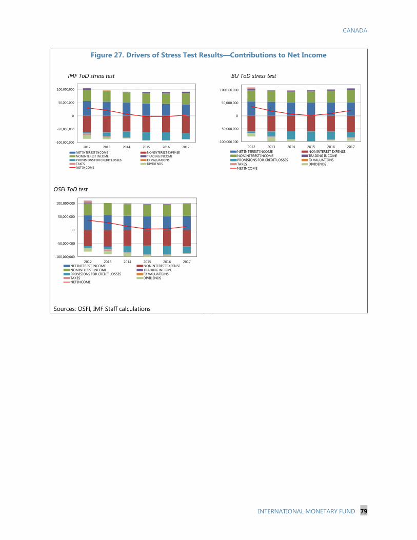
CANADA
INTERNATIONAL MONETARY FUND 79
-100,000,000
-50,000,000
0
50,000,000
100,000,000
2012 2013 2014 2015 2016 2017
NET INTEREST INCOME NONINTEREST EXPENSENONINTEREST INCOME TRADING INCOMEPROVISIONS FOR CREDIT LOSSES FX VALUATIONSTAXES DIVIDENDSNET INCOME
-100,000,000
-50,000,000
0
50,000,000
100,000,000
2012 2013 2014 2015 2016 2017NET INTEREST INCOME NONINTEREST EXPENSENONINTEREST INCOME TRADING INCOMEPROVISIONS FOR CREDIT LOSSES FX VALUATIONSTAXES DIVIDENDSNET INCOME
-100,000,000
-50,000,000
0
50,000,000
100,000,000
2012 2013 2014 2015 2016 2017NET INTEREST INCOME NONINTEREST EXPENSENONINTEREST INCOME TRADING INCOMEPROVISIONS FOR CREDIT LOSSES FX VALUATIONSTAXES DIVIDENDSNET INCOME
Figure 27. Drivers of Stress Test Results—Contributions to Net Income
IMF ToD stress test
BU ToD stress test
OSFI ToD test
Sources: OSFI, IMF Staff calculations

CANADA
80 INTERNATIONAL MONETARY FUND
75,000,000 77,000,000 79,000,000 81,000,000 83,000,000
85,000,000 87,000,000 89,000,000 91,000,000 93,000,000
2012 2013 2014 2015 2016 2017IMF top down OSFI top down Bottom up
29,000,000
31,000,000
33,000,000
35,000,000
37,000,000
39,000,000
41,000,000
43,000,000
2012 2013 2014 2015 2016 2017IMF top down OSFI top down Bottom up
35,000,000
40,000,000
45,000,000
50,000,000
2012 2013 2014 2015 2016 2017IMF top down (does not include trading income)OSFI top downBottom up
54,000,000
56,000,000
58,000,000
60,000,000
62,000,000
64,000,000
66,000,000
2012 2013 2014 2015 2016 2017IMF top down OSFI top down Bottom up
-6,000,000
-4,000,000
-2,000,000
-
2,000,000
4,000,000
6,000,000
8,000,000
2012 2013 2014 2015 2016 2017
IMF top down (includes gains in P&L and OCE items)OSFI top downBottom up
-
5,000,000
10,000,000
15,000,000
20,000,000
25,000,000
30,000,000
35,000,000
40,000,000
2012 2013 2014 2015 2016 2017
IMF top down (minus LLR) OSFI top down Bottom up
Figure 28. Net Income and RWAs—Comparison
Interest income Interest expense
Non-interest income Non-interest expense
Trading income Charge for impairment
Sources: OSFI, IMF Staff calculations

CANADA
INTERNATIONAL MONETARY FUND 81
-3,000,000 -2,000,000 -1,000,000
-1,000,000 2,000,000 3,000,000 4,000,000 5,000,000 6,000,000 7,000,000 8,000,000
2012 2013 2014 2015 2016 2017
IMF top down OSFI top down Bottom up
-10,000,000
-
10,000,000
20,000,000
30,000,000
40,000,000
2012 2013 2014 2015 2016 2017
IMF top down (comprehensive income)
OSFI top down
Bottom up
-5,500,000
-500,000
4,500,000
9,500,000
14,500,000
19,500,000
2012 2013 2014 2015 2016 2017
IMF top down OSFI top down Bottom up
800,000,000
1,000,000,000
1,200,000,000
1,400,000,000
1,600,000,000
1,800,000,000
2,000,000,000
2012 2013 2014 2015 2016 2017
IMF top down OSFI top down Bottom up
60,000,000
65,000,000
70,000,000
75,000,000
80,000,000
85,000,000
90,000,000
95,000,000
100,000,000
2012 2013 2014 2015 2016 2017IMF top down OSFI top down Bottom up
140,000,000
145,000,000
150,000,000
155,000,000
160,000,000
165,000,000
170,000,000
2012 2013 2014 2015 2016 2017IMF top down OSFI top down Bottom up
Figure 29. Net Income and RWAs—Comparison Taxes Net income after taxes
Dividends RWAs for credit risk
RWAs for market risk RWAs for operational risk
Sources: OSFI, IMF Staff calculations

CANADA
82 INTERNATIONAL MONETARY FUND
0.0
1.0
2.0
3.0
4.0
5.0
2012 2013 2014 2015 2016 2017IMF top downOSFI top downBottom upIMF top down (TTC PDs, regulatory RWAs)
0.0
10.0
20.0
30.0
40.0
50.0
60.0
2012 2013 2014 2015 2016 2017IMF top down OSFI top down
Bottom up IMF top down (stressed LRDEs)
0
0.05
0.1
0.15
0.2
0.25
0.3
0.35
1997 1999 2001 2003 2005 2007 2009 2011 2013 2015 2017Agriculture Construction / Real estateManufacturing Retail / Small business loansWholesale trade Accommodations (service)Consumer loans Residential mortgages
0.0
1.0
2.0
3.0
4.0
5.0
2012 2013 2014 2015 2016 2017IMF top downOSFI top downBottom upIMF top down (TTC PDs, regulatory RWAs)
Figure 30. Parameters of RWAs and Expected Losses—Comparison
Weighted average PDs, in % Weighted average LGDs, in %
Sectoral PDs
Exposure growth
Sources: OSFI, BoC, IMF Staff calculations
-6.0%
-4.0%
-2.0%
0.0%
2.0%
4.0%
6.0%
8.0%
2013 2014 2015 2016 2017
IMF top down OSFI top downBottom up Bottom up (Basel II)BoC credit growth forecast

CANADA
INTERNATIONAL MONETARY FUND 83
0.0%
5.0%
10.0%
15.0%
20.0%
25.0%
30.0%
35.0%
2012 2013 2014 2015 2016 2017
IMF top down OSFI top down Bottom up
0.0%
1.0%
2.0%
3.0%
4.0%
5.0%
6.0%
7.0%
8.0%
2012 2013 2014 2015 2016 2017IMF top down OSFI top down Bottom up
Figure 31. Recapitalization Needs—as Percent in gross income
Recapitalization needs to reach supervisory threshold
Recapitalization needs to reach regulatory threshold
Sources: OSFI, IMF Staff calculations
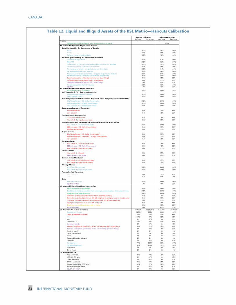
CANADA
84 INTERNATIONAL MONETARY FUND
Bad state Good state Bad state Good stateA. Cash
Deposits with Bank of Canada, bank notes and items in transitB1. Marketable Securities/Liquid assets- Canada
Securities issued by the Government of CanadaT-bills 98% 100%Bonds 98% 100%Stripped coupons and residuals 98% 100%
Securities guaranteed by the Government of CanadaCanada Mortgage Bonds 97% 100%NHA MBS 97% 100%Government of Canada guaranteed stripped coupons and residuals 96% 100%Securities issued by a provincial government 96% 100%Provincial government - stripped coupons and residuals 94% 100%Securities guaranteed by a province 96% 100%Provincial government guaranteed - stripped coupons and residuals 94% 100%Securities issued by a Municipal government (High Rating) 95% 100%Securities issued by a Municipal government (Low Rating) 75% 85%Corporate and foreign-issuer bonds (High Rating) 75% 85%Corporate and foreign-issuer bonds (Low Rating) 40% 50%Securities issued by the U.S. Treasury 96% 100%Equities 40% 50%
B2. Marketable Securities/Liquid assets- USATotal Cash and Cash Equivalents 100% 100%
U.S. Treasuries & Fully Guaranteed AgenciesBill/Notes/Bonds/Inflation Indexed 100% 100%Zero Coupon, STRIPs 100% 100%
FDIC Temporary Liquidity Guarantee Program & NCUA Temporary Corporate Credit UnBills/Notes/Bonds - U.S. Dollar Denominated 100% 100%Bills/Notes/Bonds - Foreign Denominated7 100% 100%Zero Coupon - U.S. Dollar Denominated 100% 100%
Government Sponsored EnterprisesBills/Notes/Bonds 75% 85%Zero Coupon 75% 85%
Foreign Government AgenciesU.S. Dollar Denominated 75% 85%AAA rated - Foreign Denominated 75% 85%
Foreign Government, Foreign Government Guaranteed, and Brady BondsAAA rated - U.S. Dollar Denominated 100% 100%BBB-AA rated - U.S. Dollar Denominated 75% 85%Foreign Denominated 75% 85%
Supranationals Bills/Notes/Bonds - U.S. Dollar Denominated 75% 85%Bills/Notes/Bonds - AAA rated - Foreign Denominated7 75% 85%Zero Coupon 75% 85%
Corporate BondsAAA rated - U.S. Dollar Denominated 75% 85%BBB-AA rated - U.S. Dollar Denominated 40% 50%AAA rated - Foreign Denominated 75% 85%
Covered Bonds AAA rated - U.S. Issued 75% 85%BBB-AA rated - U.S. Issued 40% 50%
German Jumbo PfandbriefeAAA rated - U.S. Dollar Denominated 75% 85%AAA rated - Foreign Denominated7 75% 85%
Municipal BondsU.S. Dollar Denominated 100% 100%AAA rated - Foreign Denominated 100% 100%
Agency Backed MortgagesPass Throughs 50% 75%CMOs 50% 75%
OtherTerm deposit facility 100% 100%Equity securities 40% 50%
B3. Marketable Securities/Liquid assets- OtherTotal Cash and Cash Equivalents 100% 100%Qualifying marketable securities from sovereigns, central banks, public sector entities, 100% 100%Qualifying central bank reserves 100% 100%Domestic sovereign or central bank debt in domestic currency 75% 85%Domestic sovereign debt for non-0% risk weighted sovereigns, issues in foreign curre 75% 85%Sovereign, central banks and PSE assets qualifying for 20% risk weighting 75% 85%Qualifying corporate bonds rated AA- or higher 75% 85%Qualifying covered bonds rated AA- or higher 75% 85%Equity securities 40% 50%
C1. Iliquid assets- various currencies Bad state Good state Bad state Good stateDeposits with banks 100% 100% 100% 100%Other government securities 50% 85% 50% 85%MBS 50% 75% 50% 75%ABS 0% 40% 0% 40%Corporate CP 50% 85% 50% 85%Corporate bonds 0% 40% 0% 40%Bankers' acceptances, promissory notes, commercial paper (High Rating) 50% 85% 50% 85%Bankers' acceptances, promissory notes, commercial paper (Low Rating) 0% 50% 0% 50%Precious metals 0% 0% 0% 0%Other commodities 0% 0% 0% 0%Loans 0% 0% 0% 0%Swapped Intra-bank Loans 0% 0% 0% 0%Call Loans 0% 50% 0% 50%Reverse repos 90% 100% 90% 100%Securities borrowed 90% 100% 90% 100%Derivatives 0% 0% 0% 0%Other Assets 0% 0% 0% 0%
C2. Iliquid assets- USABS AAA rated 25% 60% 25% 60%ABS BBB-AA rated 0% 40% 0% 40%CDO- AAA rated 0% 40% 0% 40%CMBS- AAA rated 25% 60% 25% 60%Private label CMOs- AAA rated 50% 75% 50% 75%Trust preferred securities 0% 40% 0% 40%CD, BA, CP, ABCP 0% 85% 0% 85%
Adverse calibration
100%
50%
85%85%85%
Baseline calibration
100%100%100%
100%100%100%100%100%100%100%100%85%85%50%100%
85%85%
85%85%
100%85%85%
100%
100%100%
100%100%100%
85%50%85%
85%50%
85%85%
100%100%
75%75%
100%50%
50%
100%100%100%85%85%85%85%85%
Table 12. Liquid and Illiquid Assets of the BSL Metric—Haircuts Calibration

CANADA
INTERNATIONAL MONETARY FUND 85
Deposits Baseline AdverseDemand / Notice Deposits
RetailPrimary Deposits (relationship)
Insured chequing 3% 5% Insured investment savings accounts 3% 5% Uninsured deposits 5% 8%
Other Deposits (non-relationship)Insured investment savings accounts 5% 8%Uninsured investment savings accounts 10% 15%Others 10% 15%
Small Business EnterprisesPrimary Deposits
Insured demand / chequing 5% 8%Uninsured deposits 10% 15%
Other Deposits (non-relationship)Insured demand / chequing 10% 15%Uninsured 10% 15%Others 10% 15%
Term DepositsRetail
Primary Deposits (relationship)Fixed Term 3% 5%Cashable 3% 5%Uninsured deposits 5% 8%
Other Deposits (non-relationship)Fixed Term 5% 8%Cashable 5% 8%Others (i.e. uninsured deposits) 10% 15%
Small Business EnterprisesPrimary Deposits (relationship)
Fixed Term 5% 8%Cashable 5% 8%Uninsured deposits 10% 15%
Other Deposits (non-relationship)Fixed Term 10% 15%Cashable 10% 15%Others (i.e. uninsured deposits) 10% 15%
Wholesale FundingWholesale Demand/Notice Deposits
Corporate/Commercial deposits 25% 50%Other 100% 100%
FinancialSecured 25% 50%Unsecured 100% 100%
Other wholesaleSecured 25% 50%Unsecured 40% 80%
Maturing funding from FI sponsored ABCP & securitization 100% 100%Swapped Intra-bank Deposits 100% 100%Other Liabilities
Banker's Acceptances 100% 100%Repurchase Agreements 100% 100%Securities lent 100% 100%Securities sold short 100% 100%Derivatives related amounts 0% 0%Others 0% 0%
LCR Category D. (off-balance sheet items)Liquidity needs related to downgrade triggers embedded in financing 100% 100% transactions, derivatives and other contracts (up to 3 notch downgrade)Market valuation changes on derivatives transactions (largest absolute 100% 100% net 30-day collateral flows realised during the preceding 24 months)Valuation changes on non-Level 1 posted collateral securing derivatives 20% 40%Excess collateral held by a bank related to derivative transactions that could contractually be called at any time by its counterparty Liquidity needs related to collateral contractually due from the reporting 100% 100% bank on derivatives transactions Increased liquidity needs related to derivative transactions that allow 100% 100% collateral substitution to non-HQLA assets ABCP, SIVs, conduits, SPVs, etc:
Liabilities from maturing ABCP, SIVs, SPVs, etc (applied to maturing amounts and returnable assets) Asset Backed Securities (including covered bonds) applied to maturing amounts.
Currently undrawn committed credit and liquidity facilities provided to:retail and small business clients 5% 10%non-financial corporates, sovereigns and central banks, multilateral 10% 20% development banks, and PSEs 30% 60%banks subject to prudential supervision 40% 80%other financial institutions (include securities firms, insurance 40% 80%companies) 100% 100%other legal entity customers, credit and liquidity facilities 100% 100%
Other contingent funding liabilities (such as guarantees, letters of credit,revocable credit and liquidity facilities, etc)
Trade finance 5% 10%Customer short positions covered by other customers’ collateral
Any additional contractual outflows Net derivative cash outflows 100% 100%Any additional contractual outflows
Already included in Assets
Table 13. Outflows of BSL Metric—Run-off Rates Calibration
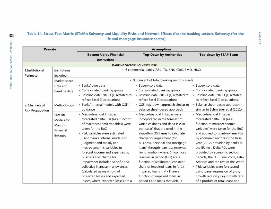
86 INTERN
ATION
AL MO
NETARY FU
ND
CANAD
A
Table 14. Stress Test Matrix (STeM): Solvency and Liquidity Risks and Network Effects (for the banking sector), Solvency (for the life and mortgage insurance sector)
Domain
Assumptions
Bottom-Up by Financial Institutions
Top-Down by Authorities Top-down by FSAP Team
BANKING SECTOR: SOLVENCY RISK
1.Institutional Perimeter
Institutions included
6 commercial banks (RBC, TD, BNS, CIBC, BMO, NBC)
Market share 93 percent of total banking sector’s assets
Data and baseline date
Banks’ own data Consolidated banking group Baseline date: 2012 Q4, restated to
reflect Basel III calculations
Supervisory data Consolidated banking group Baseline date: 2012 Q4, restated to
reflect Basel III calculations
Supervisory data Consolidated banking group Baseline date: 2012 Q4, restated
to reflect Basel III calculations.
2. Channels of Risk Propagation
Methodology Banks’ internal models with OSFI guidance
OSFI top-down approach similar to balance sheet-based approach
Balance sheet-based approach similar to Schmieder et al (2011)
Satellite Models for Macro-Financial linkages
Macro-financial linkages: forecasted delta PDs (as a function of macroeconomic variables) were taken for the BoC
P&L variables were estimated using banks’ internal models or judgment and mostly use macroeconomic variables to forecast income and expenses by business line; charge for impairment included specific and collective increase in allowances (calculated as maximum of projected losses and expected losses, where expected losses are a
Macro-financial linkages were incorporated in the forecast of variables (loans and delta PDs in particular) that are used in the algorithm OSFI uses to calculate charge for impairment (for business, personal and mortgage loans) through loan loss reserves law of motion where: (i) loan loss reserves in period (t+1) are a function of (calibrated) constant share of impaired loans in (t+1); impaired loans in (t+1) are a function of impaired loans in period t and loans that default
Macro-financial linkages: forecasted delta PDs (as a function of macroeconomic variables) were taken for the BoC and applied to point-in-time PDs by economic sectors in the base year (2012) provided by banks in the BU test; Delta PDs were provided by economic sectors in Canada, the U.S., Euro Zone, Latin America and the rest of the World
P&L variables were forecasted using panel regression of y-o-y growth rate on y-o-y growth rate of a product of total loans and

INTERN
ATION
AL MO
NETARY FU
ND
87
CANAD
A
Domain
Assumptions Bottom-Up by Financial
Institutions Top-Down by Authorities Top-down by FSAP Team
product of point-in-time PDs (forecasted PDs provided by the BoC applied to point-in-time PD in 2012), stressed LGDs (forecasted by banks but consistent with stress scenario) and exposures (drawn and undrawn) ) and increase in collective for unidentified losses determined by judgment; Exposures were reported by economic sectors in Canada, the U.S., Euro Zone, Latin America and the rest of the World; Mark-to-market gains or losses for available-for-sale (AFS) securities were projected to be consistent with the financial variables defined in the Baseline and Stress scenarios and reflected in the accumulated other comprehensive income in the Shareholders’ Equity.
during period t (depend on delta PDs provided by the BoC) net of write-offs in (t+1); write-offs in period (t+1) are a function of (calibrated) constant share of impaired loans in period t
P&L variables: interest income and interest expense were projected using projected balance sheet items and corresponding interest rates; Balance sheet items were projected as a product of loans (taken from the stress scenario) or deposits (function of nominal GDP) and a (constant) share of each balance sheet item and loans (assets item) or deposits (liabilities item) in the base year. Trading income was projected as a product of projected securities on the asset side and the share of trading income and securities which was set, in 2013, to the average loss observed over the last ten years and, in 2014-2017 to the minimum value observed in the last ten years when banks’ had positive trading income. Similar logic was
loan interest rates (for interest income), product of total deposits and deposit interest rates (for interest expense), equity prices and nominal GDP (for trading income), CAD/USD exchange rate (for FX valuations) as an explanatory variables and fixed effects. Non-interest income was projected as an average share of nominal GDP in the last 10 years. Non-interest expenses were projected as an average share of the balance sheet, assuming that balance sheet growth rate is equal to the growth rate of loans; Projections of explanatory variables were taken from the scenarios; Charge for impairment was calculated as a product of forecasted default rates, downturn LGDs provided by OSFI and exposures provided by banks in the bottom-up exercise.

88 IN
TERNATIO
NAL M
ON
ETARY FUN
D
CANAD
A
Domain
Assumptions Bottom-Up by Financial
Institutions Top-Down by Authorities Top-down by FSAP Team
applied to project non-interest income and non-interest expense.
Stress test horizon
2013-2017
3. Tail shocks Scenario analysis
Baseline: January 2013 WEO baseline, real GDP growth for 2013 is 1.7 percent and 2.3 percent for 2014 Adverse: Model-driven scenario was generated using the BoC model to simulate a U-shaped recession over
2013-2015, which represents the most severe recession in at least the last 35 years, driven by: (i) a large foreign demand shock and decreasing commodities prices caused by a disorderly default in a peripheral euro area country and a subsequent recession in the euro area and the United States, (iii) rising funding costs due to rising uncertainty and adverse confidence, (iv) negative wealth effects affecting households and business. The paths under the stress scenario of other relevant macroeconomic and financial variables are generated by the central bank using its own macroeconomic models.
Sensitivity analysis
Credit risk shocks: increase obligor correlation by 25 percent on a relative basis
Interest rate risk in the banking book: steepening of the yield curve depending on currency (e.g., 100 bps widening in the short end of the curve; 350 bps widening in the long end of the curve for CAD)
Market risk shocks on Trading, AFS securities and CVA: (i) 10 percent depreciation of the CAD against the U.S. dollar, 11 percent depreciation of the euro against the U.S. dollar, 13 percent depreciation of the GBP against
N.A. Downturn LGDs were subject to additional shock to follow the dynamics of projected LGDs by banks in the BU test- new downturn LGDs were used for calculation of expected losses and RWAs for credit risk
Negative asset correlation was replaced by positive asset correlation in the IRB formula
Point-in-time PDs were replaced by through-the-cycle PDs updated to reflect point-in-time PDs in 2013-2017
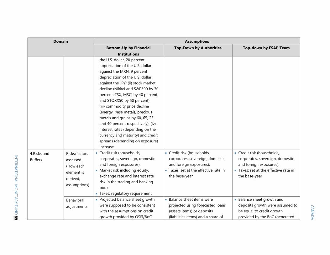
INTERN
ATION
AL MO
NETARY FU
ND
89
CANAD
A
Domain
Assumptions Bottom-Up by Financial
Institutions Top-Down by Authorities Top-down by FSAP Team
the U.S. dollar, 20 percent appreciation of the U.S. dollar against the MXN, 9 percent depreciation of the U.S. dollar against the JPY; (ii) stock market decline (Nikkei and S&P500 by 30 percent; TSX, MSCI by 40 percent and STOXX50 by 50 percent); (iii) commodity price decline (energy, base metals, precious metals and grains by 60, 65, 25 and 40 percent respectively); (iv) interest rates (depending on the currency and maturity) and credit spreads (depending on exposure) increase
4.Risks and Buffers
Risks/factors assessed (How each element is derived, assumptions)
Credit risk (households, corporates, sovereign, domestic and foreign exposures).
Market risk including equity, exchange rate and interest rate risk in the trading and banking book
Taxes: regulatory requirement
Credit risk (households, corporates, sovereign, domestic and foreign exposures).
Taxes: set at the effective rate in the base-year
Credit risk (households, corporates, sovereign, domestic and foreign exposures).
Taxes: set at the effective rate in the base-year
Behavioral adjustments
Projected balance sheet growth were supposed to be consistent with the assumptions on credit growth provided by OSFI/BoC
Balance sheet items were projected using forecasted loans (assets items) or deposits (liabilities items) and a share of
Balance sheet growth and deposits growth were assumed to be equal to credit growth provided by the BoC (generated
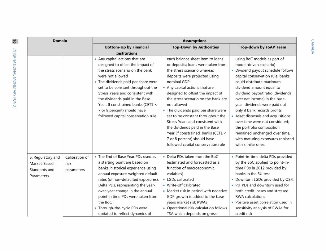
90 IN
TERNATIO
NAL M
ON
ETARY FUN
D
CANAD
A
Domain
Assumptions Bottom-Up by Financial
Institutions Top-Down by Authorities Top-down by FSAP Team
Any capital actions that are designed to offset the impact of the stress scenario on the bank were not allowed
The dividends paid per share were set to be constant throughout the Stress Years and consistent with the dividends paid in the Base Year. If constrained banks (CET1 < 7 or 8 percent) should have followed capital conservation rule
each balance sheet item to loans or deposits; loans were taken from the stress scenario whereas deposits were projected using nominal GDP
Any capital actions that are designed to offset the impact of the stress scenario on the bank are not allowed
The dividends paid per share were set to be constant throughout the Stress Years and consistent with the dividends paid in the Base Year. If constrained, banks (CET1 < 7 or 8 percent) should have followed capital conservation rule
using BoC models as part of model-driven scenario)
Dividend payout schedule follows capital conservation rule; banks could distribute maximum dividend amount equal to dividend payout ratio (dividends over net income) in the base-year; dividends were paid out only if bank records profits.
Asset disposals and acquisitions over time were not considered; the portfolio composition remained unchanged over time, with maturing exposures replaced with similar ones.
5. Regulatory and Market-Based Standards and Parameters
Calibration of risk parameters
The End of Base Year PDs used as a starting point are based on banks’ historical experience using annual exposure-weighted default rates (of non-defaulted exposures). Delta PDs, representing the year-over-year change in the annual point in time PDs were taken from the BoC
Through-the-cycle PDs were updated to reflect dynamics of
Delta PDs taken from the BoC (estimated and forecasted as a function of macroeconomic variables)
LGDs calibrated Write-off calibrated Market risk in period with negative
GDP growth is added to the base years market risk RWAs
Operational risk calculation follows TSA which depends on gross
Point-in-time delta PDs provided by the BoC applied to point-in-time PDs in 2012 provided by banks in the BU test
Downturn LGDs provided by OSFI PIT PDs and downturn used for
both credit losses and stressed RWA calculations
Positive asset correlation used in sensitivity analysis of RWAs for credit risk

INTERN
ATION
AL MO
NETARY FU
ND
91
CANAD
A
Domain
Assumptions Bottom-Up by Financial
Institutions Top-Down by Authorities Top-down by FSAP Team
point-in-time PDs For calculation of RWAs for credit
risk, banks projected changes in the credit quality of their exposures consistent with the various macroeconomic and financial factors provided in the Baseline and Stress scenarios (for example, IRB banks were allowed to move exposures into different IRB LGD/PD buckets in a fashion consistent with the stress scenario, but were not allowed to recalibrate IRB LGDs or through-the-cycle PDs)
The calculation of Market Risk RWA considered the following points: VaR: During a period of negative GDP growth rates, VaR was set to the Base Year Stressed VaR, and during a period of positive GDP growth rates, VaR was set to the level of the Base Year VaR. Stressed VaR: Stress VaR remained constant at the base year Stressed VaR level.
income
Regulatory/Accounting and
Hurdle rate: Basel III schedule (regulatory minimum), and local
Hurdle rate: Basel III schedule (regulatory minimum), and local
Hurdle rate: Basel III schedule (regulatory minimum), and local

92 IN
TERNATIO
NAL M
ON
ETARY FUN
D
CANAD
A
Domain
Assumptions Bottom-Up by Financial
Institutions Top-Down by Authorities Top-down by FSAP Team
Market-Based Standards
regulatory requirements (“all in”, supervisory minimum)
regulatory requirements (“all in”, supervisory minimum)
regulatory requirements (“all in”, supervisory minimum)
Capital metrics: “all-in” Basel III, and local regulatory requirements
“all-in” CET1, T1, CAR
Capital metrics: “all-in” Basel III, and local regulatory requirements
“all-in” CET1
Capital metrics: “all-in” Basel III, and local regulatory requirements.) “all-in” CET1, T1, CAR
Risk-weighted assets for credit risk: calculated for standardized and IRB exposures; , banks projected changes in the credit quality of their exposures consistent with the various macroeconomic and financial factors provided in the Baseline and Stress scenarios (for example, IRB banks were allowed to move exposures into different IRB LGD/PD buckets in a fashion consistent with the stress scenario, but were not allowed to recalibrate IRB LGDs or through-the-cycle PDs); through-the-cycle PDs were updated to reflect dynamics of point-in-time PDs
The calculation of Market Risk
Risk-weighted assets were modeled using two approaches: (i) by applying risk weights from 2012 BU stress test in the stress scenario, and (ii) using IRB formulas by asset classes assuming there are no standardized exposures using downturn LGDs, through-the-cycle PDs and exposures reported by banks in the BU test
Market risk in period with negative GDP growth is added to the base years market risk RWAs
Operational risk calculation follows TSA which depends on gross income
Risk-weighted assets: For computation of credit risk, RWAs under stress for each bank by asset classes were calculated using Basel II, IRB formula that translates downturn LGDs, changes in point-in-time PDs, changes in assets correlation and the maturity adjustment parameter into stressed RWAs in economic terms. “Standardized exposures” were added to “IRB exposures” to calculate total exposures by asset classes. Percentage changes in calculated RWAs was applied to the base year, real RWAs65- levels of calculated RWAs will were not used in a calculation of capital
65 Note that we have necessary data to calculate percentage change of RWAs in 2013 using calculated levels of RWAs in 2013 and 2012.

INTERN
ATION
AL MO
NETARY FU
ND
93
CANAD
A
Domain
Assumptions Bottom-Up by Financial
Institutions Top-Down by Authorities Top-down by FSAP Team
RWA should consider the following points: VaR: During a period of negative GDP growth rates, VaR should be set to the Base Year Stressed VaR, and during a period of positive GDP growth rates, VaR should be set to the level of the Base Year VaR. Stressed VaR: Stress VaR should remain constant at the base year Stressed VaR level.
Banks recalculated the charge for operational risk to be consistent with the Baseline and Stress scenarios. For banks using the Standardized Approach (“TSA”), the derivation of the charge reflected Gross Income consistent with the earnings projections provided in the Income Statement supporting schedules for the relevant years of the scenario
Full implementation of the CVA charge- RWAs for CCR and CVA were calculated based on Basel III rules; Banks treated all CCPs as QCCPs unless they have reason to believe otherwise; The Current
requirements; In the sensitivity analysis we shocked downturn LGDs to follow the dynamics of LGDs projected by the banks; we replaced negative asset correlation with positive one and we used trough-the cycle PDs provided by OSFI.
RWAs for market and operational risk were taken from the banks, reported for the BU test.

94 IN
TERNATIO
NAL M
ON
ETARY FUN
D
CANAD
A
Domain
Assumptions Bottom-Up by Financial
Institutions Top-Down by Authorities Top-down by FSAP Team
Exposure Method (CEM) was used for calculating CCR RWA, and the Standardized CVA capital charge with CEM-based EAD was used to calculate CVA capital requirements.
BANKING SECTOR: LIQUIDITY RISK 1.Institutional Perimeter
Institutions included
N.A. 6 commercial banks (RBC, TD, BNS, CIBC, BMO, NBC)
N.A.
Market share N.A. 93 percent of total banking sector’s assets
N.A.
Data and baseline date
N.A. Data provided by banks for liquidity tests
Consolidated banking group as of April 2013.
N.A.
2. Channels of Risk Propagation
Methodology N.A. MFRAF: funding liquidity risk (and network effects) is modeled as an endogenous outcome of the interaction between market liquidity risk, solvency risk and the structure of banks’ funding under the baseline and the adverse scenario; liquidity (and network effects) are translated into losses that affect capital position of each bank
N.A.

INTERN
ATION
AL MO
NETARY FU
ND
95
CANAD
A
Domain
Assumptions Bottom-Up by Financial
Institutions Top-Down by Authorities Top-down by FSAP Team
3. Tail shocks Size of the shock
N.A. The shock is endogenous and is represented by a run by short-term creditors conditional on the size of credit losses and liquidity measure which depend on calibrated fire-sales discounts, amount of liquid and illiquid assets and the value of liabilities maturing over the next 6 months; calibrated parameters of the liquidity measure are in large part consistent with parameters of revised Basel III LCR haircuts (on the asset side) and run-off rates (on the funding side).
N.A.
4.Risks and Buffers
Risks N.A. Funding and market liquidity risk (including information contagion risk) due to solvency issues
N.A.
Buffers N.A. Liquid assets N.A.
5. Regulatory and Market-Based Standards and Parameters
Calibration of risk parameters
N.A. Parameters are calibrated based on banks’ monthly balance sheet reports; Parameters of the liquidity measure are, in large part, consistent with the revised Basel III LCR; liquidity losses are assumed
N.A.

96 IN
TERNATIO
NAL M
ON
ETARY FUN
D
CANAD
A
Domain
Assumptions Bottom-Up by Financial
Institutions Top-Down by Authorities Top-down by FSAP Team
to be equal to 2.25% of RWAs
Regulatory standards
N.A. The “run point” is an increasing function of bank’s capital, liquid asset holdings, and the return on short-term debt and a decreasing function of the amount of short-term funding and the opportunity cost of short-term creditors
N.A.
BANKING SECTOR: SPILLOVER RISKS 1.Institutional Perimeter
Institutions included
N.A. 6 commercial banks (RBC, TD, BNS, CIBC, BMO, NBC)
N.A.
Market share N.A. 93 percent of total banking sector’s assets
N.A.
Data and baseline date
N.A. Data provided by banks in regulatory return on interbank exposures (exposures that arise from traditional lending estimated by entropy maximization algorithm, cross-shareholdings and off-balance sheet instruments such as exchange traded and OTC derivatives from OSFI’s Survey)
Consolidated banking group as of April 2013.
N.A.
2. Channels of Risk Propagation
Methodology N.A. MFRAF: includes network externalities caused by counterparties’ default which depend on credit losses and losses
N.A.

INTERN
ATION
AL MO
NETARY FU
ND
97
CANAD
A
Domain
Assumptions Bottom-Up by Financial
Institutions Top-Down by Authorities Top-down by FSAP Team
caused by market and funding liquidity disruptions
3. Tail shocks Size of the shock
N.A. Defaulting banks are unable to fully honor their interbank liabilities
N.A.
4. Risks Risks N.A. Spillover risks/default N.A.
LIFE INSURANCE SECTOR: SOLVENCY RISKS 1.Institutional Perimeter
Institutions included
3 largest life insurers, Sunlife Financial, Great West Lifeco, and Manulife Financial
N.A. N.A.
Market share Over 60 percent of premiums written in 2012.
N.A. N.A.
Data and baseline date
Insurers’ own data Baseline date: 2012Q4
N.A. N.A.
2. Channels of Risk Propagation
Methodology Insurers’ internal models with OSFI guidance
N.A.
N.A.
Stress test horizon
2013-2017 N.A.
N.A.
3. Tail shocks Scenario analysis
Same stress scenario was applied as in the banking sector stress test
N.A.
N.A.
Sensitivity analysis
Credit spread shocks: increase in Canadian, U.S., and European issuers’ spreads identical to the
N.A.
N.A.

98 IN
TERNATIO
NAL M
ON
ETARY FUN
D
CANAD
A
Domain
Assumptions Bottom-Up by Financial
Institutions Top-Down by Authorities Top-down by FSAP Team
calibrations for the bottom-up analysis by banks: up to 3-4 the level of end-2012 credit spreads for 2013, gradually declining in the following years
Interest rate risk: decline in CAD, USD, Bund, and JPY interest rates in 2013, gradual increase from 2014 onwards
Equity index shocks: stock market decline (Nikkei and S&P500 by 30 percent; TSX, MSCI by 40 percent and STOXX50 by 50 percent);
Currency valuation shocks: 10 percent depreciation of the CAD against the U.S. dollar, 11 percent depreciation of the euro against the U.S. dollar, 13 percent depreciation of the GBP against the U.S. dollar, 20 percent appreciation of the U.S. dollar against the MXN, 9 percent depreciation of the U.S. dollar against the JPY
Policy holder behavior: stressed lapse rates, 20 percent higher than in baseline scenario
Combined effect of all shocks

INTERN
ATION
AL MO
NETARY FU
ND
99
CANAD
A
Domain
Assumptions Bottom-Up by Financial
Institutions Top-Down by Authorities Top-down by FSAP Team
above.
4.Risks and Buffers
Risks/factors assessed
Credit risk (federal and provincial governments /agencies, corporates, domestic and foreign exposures).
Market risk including equity, exchange rate and interest rate risk
N.A.
N.A.
Buffers Capital N.A. N.A.
MORTGAGE INSURANCE: SOLVENCY RISKS 1.Institutional Perimeter
Institutions included
Large mortgage insurance company. N.A. N.A.
Data and baseline date
Financial institution provided own data Baseline date: 2012Q4
N.A. N.A.
2. Channels of Risk Propagation
Methodology Financial institution’s internal models with OSFI guidance
N.A.
N.A.
Stress test horizon
2013-2017
3. Tail shocks Scenario analysis
Same stress scenario was applied as in the banking sector stress test
N.A.
N.A.
Sensitivity analysis
Same as life insurers (except for higher lapses)
N.A.
N.A.
4.Risks and Buffers
Risks Credit risk (mortgage loans) Market risk including equity, exchange
rate and interest rate risk
N.A.
N.A.
Buffers Capital N.A. N.A.

CANADA
100 INTERNATIONAL MONETARY FUND
References
Christensen, I., P. Corrigan, C. Mendicino, and S.-I. Nishiyama, 2009, “Consumption, Housing
Collateral, and the Canadian Business Cycle?," Bank of Canada, Working Paper 2009-26. Christensen, I. and C. A. Meh, 2011, “Countercyclical loan-to-value ratios and monetary policy”,
Bank of Canada, mimeo. Faruqui U., X. Liu and T. Roberts, 2012, ”An Improved Framework for Assessing the Risks Arising
from Elevated Household Debt”, Bank of Canada Financial Stability Review, June, pp 51–57.
Fitch, 2008, “Basel II Correlation Values, An Empirical Analysis of EL, UL and the IRB Model”,
Credit Market Research Financial Institutions Special Report. Gauthier, C., Z. He and M. Souissi, 2010, “Understanding Systemic Risk: The Trade-Offs Between
Capital, Short-Term Funding and Liquid Asset Holdings.” Bank of Canada Working Paper No. 2010-29.
Gerali, A., S. Nerri, F. M. Signoretti and L. Sessa, 2010, “Credit and banking in a DSGE model of
the euro area”, Journal of Money, Credit and Banking, Vol. 42, Supplement 1, pp. 107-141.
Iacoviello, M., 2005, “House prices, borrowing constraints and monetary policy in the business
cycle," American Economic Review, 95(3), 739-764. Laurent, Marie-Paule, 2004, “How to reduce capital requirement? The case of retail portfolios
with low probability of default”, mimeo. Moody’s KMV, 2009, “The Relationship between average asset correlation and default
probability”. Morris, S., and Shin, H. Song, 2010, “Illiquidity Component of Credit Risk”, Working Paper,
Princeton University. Ramdane D. and É. Bordeleau, 2013, “Méthodologie de construction de séries de taux de défaut
pour l’industrie canadienne”, Discussion Papers 13-2, Bank of Canada. Schmieder, Christian, Puhr Claus, and Maher K. Hasan, 2011, “Next Generation Balance Sheet
Stress Testing,” IMF Working Paper No. 11/83 (Washington: International Monetary Fund).