impact analysis of options for implementing article …...final report impact analysis of options...
TRANSCRIPT

Final Report
Impact Analysis of Options for Implementing Article 7a of Directive 98/70/EC (Fuel Quality Directive)
02 August 2013
Submitted to:
Wojciech Winkler
European Commission
DG Climate Action
B-1049 Brussels
BELGIUM
Submitted by:
ICF International
3rd Floor
Kean House
6 Kean Street
London WC2B 4AS
U.K.

Impact Analysis of Options for Implementing Article 7a of Directive 98/70/EC (Fuel Quality Directive) Final Report under Contract 071201/2011/608705/SER/CLIMA.C2
August 2013 i
Table of Contents
Table of tables ................................................................................................................ iv
Table of figures ................................................................................................................. viii
1 Introduction ........................................................................................................... 1
1.1 Objectives of Project .............................................................................................. 1
1.2 This Report ............................................................................................................. 1
2 Develop Fuel Projections under Baseline Reporting (Task 1.1) ............................... 2
2.1 Introduction ........................................................................................................... 2
2.2 Literature review ................................................................................................... 2
2.3 Preliminary Assessment ......................................................................................... 3
2.4 In‐Depth Assessment ........................................................................................... 11 2.4.1 The EU Transport GHG: Routes to 2050 – Illustrative Scenarios Tool (SULTAN) ................ 11 2.4.2 The World Energy Outlook 2011 (WEO 2011) ....................................................................... 14 2.4.3 International Energy Outlook 2012 (IEO 2011) ...................................................................... 17 2.4.4 Wood Mackenzie Report ........................................................................................................ 18 2.4.5 WORLD Model ........................................................................................................................ 20 2.4.6 Overall Comments .................................................................................................................. 22
2.5 2020 Baseline Fuel Demand Projections ............................................................... 22 2.5.1 Assumptions for the 2020 Baseline Forecast Model .............................................................. 22 2.5.2 Meta-Analysis Forecast Begins with Data from IEA WEO 2011 ............................................ 24 2.5.3 Apportion Total Fuel Demand from IEA Midterm Report to the Road Transport Sector ........ 24 2.5.4 Scaled Projections to 2020 ..................................................................................................... 24 2.5.5 Incorporate Electricity and CNG Demand .............................................................................. 26 2.5.6 EC Supply of Biofuels ............................................................................................................. 28 2.5.7 2020 Baseline Demand Scenario Combination ...................................................................... 29
2.6 Feedstock and Product Projections ...................................................................... 29 2.6.1 Introduction to the WORLD Model .......................................................................................... 29 2.6.2 Key drivers of Product Trade in WORLD Model ..................................................................... 29 2.6.3 Summary of Premises for Model Run ..................................................................................... 31 2.6.4 Model Output and Results ...................................................................................................... 35 2.6.5 2020 Crude Trade ................................................................................................................... 37 2.6.6 Refinery Capacities and Utilisation ......................................................................................... 43 2.6.7 2020 Fuel Trade ..................................................................................................................... 55 2.6.8 Factors Contributing to European Diesel and Petrol Market .................................................. 56
3 Baseline GHG Emissions and GHG Intensity (Task 1.2) .......................................... 69
3.1 Introduction ......................................................................................................... 69
3.2 Scope ................................................................................................................... 69
3.3 Baseline GHG Emissions and GHG Intensity .......................................................... 69
3.4 Sensitivity Analysis including ILUC Emissions ....................................................... 74 3.4.1 Introduction to GHG Emissions from ILUC ............................................................................. 74 3.4.1 Scenario to Demonstrate Sensitivity ....................................................................................... 76
4 Costs of the Baseline (Task 1.3) ............................................................................ 78
Impact Analysis of Options for Implementing Article 7a of Directive 98/70/EC (Fuel Quality Directive) Final Report under Contract 071201/2011/608705/SER/CLIMA.C2
August 2013 ii
4.1 Introduction ......................................................................................................... 78
4.2 Scope ................................................................................................................... 78
4.3 GHG Reductions of Strategies in the Baseline Projections .................................... 78 4.3.2 Bioethanol ............................................................................................................................... 79 4.3.3 Biodiesel ................................................................................................................................. 79 4.3.4 Electricity................................................................................................................................. 79 4.3.5 CNG and LPG ......................................................................................................................... 79
4.4 Review of Marginal Abatement Costs .................................................................. 80 4.4.2 Bioethanol ............................................................................................................................... 81 4.4.3 Biodiesel ................................................................................................................................. 84 4.4.4 Electricity................................................................................................................................. 86 4.4.5 CNG and LPG ......................................................................................................................... 86 4.4.6 Flare Reduction in Upstream Production ................................................................................ 87 4.4.7 Combined MAC curve for Strategies in Baseline Projections ................................................ 89
4.5 Estimated Costs in the Baseline Fuel Projections .................................................. 90
4.6 Estimated Costs of BAU Scenario and ILUC Sensitivity Scenario ........................... 91
5 Development of options (Task 2.1) ....................................................................... 95
5.1 Introduction ......................................................................................................... 95
5.2 Description of options .......................................................................................... 95 5.2.1 Introduction ............................................................................................................................. 95 5.2.2 Key issues .............................................................................................................................. 99 5.2.3 Option 0 (Baseline / ‘do nothing’) ......................................................................................... 100 5.2.4 Option 1 (Current proposal) .................................................................................................. 101 5.2.5 Option 2 ................................................................................................................................ 105 5.2.6 Suppliers meeting the reduction obligation jointly ................................................................ 109 5.2.7 Option 3 ................................................................................................................................ 110 5.2.8 Upstream Emission Reductions ........................................................................................... 114 5.2.9 Option 4 ................................................................................................................................ 115 5.2.10 Option 5 ................................................................................................................................ 118 5.2.11 Summary of equations .......................................................................................................... 119
5.3 Supplier‐specific unit GHG intensities: Life Cycle Analysis (LCA) ......................... 120 5.3.1 Introduction ........................................................................................................................... 120 5.3.2 LCA Methods and costs ........................................................................................................ 120 5.3.3 Use of LCA in California’s Low Carbon Fuel Standard ........................................................ 123 5.3.4 LCA Stages ........................................................................................................................... 125
6 Analysis of options (Task 2.2) ............................................................................. 140
6.1 Introduction ....................................................................................................... 140
6.2 Methodology for analysis ................................................................................... 140 6.2.1 Overview and problem definition .......................................................................................... 140 6.2.2 Identification of appropriate data sources ............................................................................. 141 6.2.3 Setting up the Analysis framework ....................................................................................... 150 6.2.4 Identification of compliance measures and supplier decision making .................................. 167 6.2.5 Compliance costs ................................................................................................................. 174 6.2.6 Administrative costs .............................................................................................................. 175
6.3 Results of the analysis of policy options ............................................................. 192 6.3.1 Environmental impacts ......................................................................................................... 192

Impact Analysis of Options for Implementing Article 7a of Directive 98/70/EC (Fuel Quality Directive) Final Report under Contract 071201/2011/608705/SER/CLIMA.C2
August 2013 iii
6.3.2 Administrative impacts .......................................................................................................... 199
7 Characterisation of affected sectors (Task 3.1) ................................................... 203
7.1 Introduction to the EU refining industry ............................................................. 203
7.2 Structure of downstream industry ..................................................................... 205 7.2.1 Location and key statistics of the EU refining industry ......................................................... 205 7.2.2 Demand for refined products ................................................................................................ 211 7.2.3 Price elasticity of demand for refined product and refinery cost pass-through rates ........... 214 7.2.4 Profit margins in European refining ...................................................................................... 216 7.2.5 Complexity of EU refineries .................................................................................................. 219 7.2.6 Emissions intensity ............................................................................................................... 221 7.2.7 Trade in refined products ...................................................................................................... 224
8 Impacts of the Fuel Quality Directive on the EU road transport fuel market (Task 3.2) ........................................................................................................... 228
8.1 Introduction ....................................................................................................... 228
8.2 Main results ....................................................................................................... 229
8.3 Required emissions reduction in the EU transport fossil fuel market ................. 232
8.4 Analysis of options ............................................................................................. 233 8.4.1 Compliance cost curves ........................................................................................................ 233 8.4.2 EU transport fuel market effects ........................................................................................... 238 8.4.3 Crude market effects ............................................................................................................ 240 8.4.4 Product import market effects ............................................................................................... 240 8.4.5 Pump prices .......................................................................................................................... 241
Bibliography .................................................................................................................... 244
Appendix A – Further information on competitive impacts ............................................. 247
Appendix B ‐ Biofuel feedstock switching as an additional compliance method .............. 258
Appendix C – Pump Prices ............................................................................................... 261

Impact Analysis of Options for Implementing Article 7a of Directive 98/70/EC (Fuel Quality Directive) Final Report under Contract 071201/2011/608705/SER/CLIMA.C2
August 2013 iv
Table of tables
Table 2.1 Key characteristics for the projection ................................................................................. 2
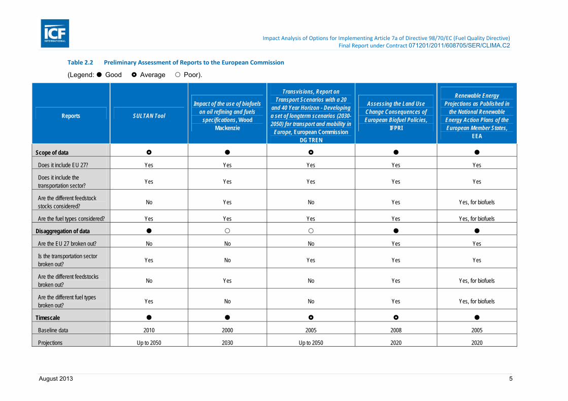
Table 2.2 Preliminary Assessment of Reports to the European Commission .................................... 5
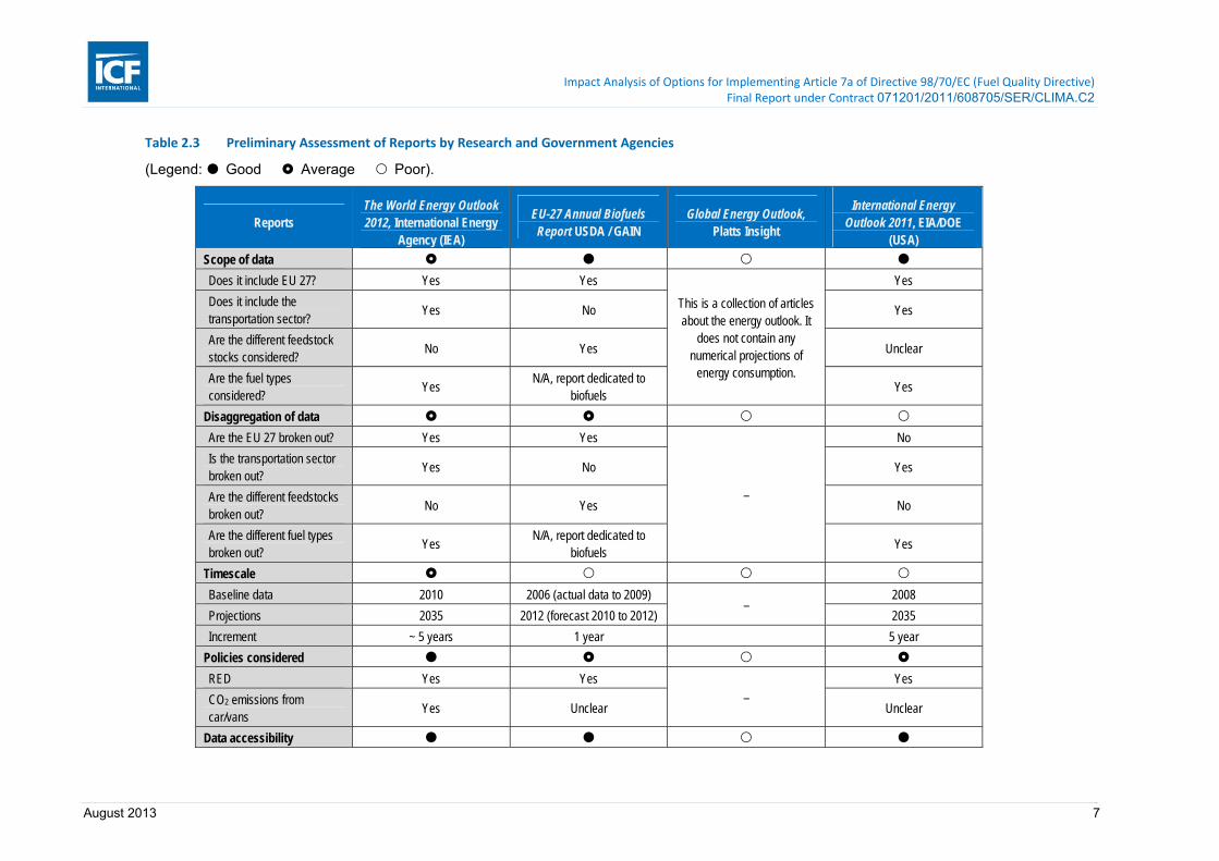
Table 2.3 Preliminary Assessment of Reports by Research and Government Agencies .................. 7
Table 2.4 Preliminary Assessment of Reports by Trade Organizations and Energy Companies ...... 9
Table 2.5 Summary of Rating for Important Reports and Studies After in-Depth Analysis .............. 11
Table 2.6 Detailed Assessment of the SULTAN Tool ...................................................................... 12
Table 2.7 Detailed Assessment of the WEO 2011 ........................................................................... 14
Table 2.8 Detailed assessment of International Energy Outlook. .................................................... 17
Table 2.9 Detailed Assessment of Wood Mackenzie Report. .......................................................... 19
Table 2.10 Detailed Assessment of WORLD Model .......................................................................... 21
Table 2.11 IEA 2009 Historical Fuel Consumption Data – Road Transport and Total ....................... 24
Table 2.12 Ratio of Specific Fuel Demand to Total Demand in 2017 Midterm .................................. 25
Table 2.13 2020 Scaled IEA Fuel Projections for EU-27 ................................................................... 25
Table 2.14 2020 Scaled IEA Fuel Projections for EU-27 Transport Sector ....................................... 25
Table 2.15 2020 On-Road Diesel and Off-Road Diesel Ratios from JEC Report .............................. 26
Table 2.16 2020 Scaled IEA Fuel Projections for EU-27 Transport Sector ....................................... 26
Table 2.17 2020 Fuel Projections for EU-27 Road Transport Sector ................................................. 27
Table 2.18 Petrol Demand in EU-27, 2006 – 2020 ............................................................................ 27
Table 2.19 Diesel Demand in EU-27, 2006 – 2020 ............................................................................ 28
Table 2.20 2020 EU-27 Road and NRMM Biofuel Supply Projections .............................................. 28
Table 2.21 Premise for WORLD Model 2020 Projections .................................................................. 32
Table 2.22 Summary of Crude Trade by Region of Origin in 2020 .................................................... 38
Table 2.23 Summary of Historical Crude Trade in 2010 .................................................................... 38
Table 2.24 Summary of Notional Crude Trade in 2020 ...................................................................... 41
Table 2.25 Announced European Refinery Closures ......................................................................... 43
Table 2.26 Summary of Refinery Projects Accounted for in the WORLD Model (‘Europe’ region) ... 44
Table 2.27 European Refinery Process Unit Capacity Utilization in 2020 ......................................... 46
Table 2.28 Global Refinery Process Unit Capacity Utilization in 2020 ............................................... 49
Table 2.29 Current structure of European refining industry ............................................................... 52
Table 2.30 EU-27 Fossil Fuel and Biofuel Consumption Road and NRMM Transport Comparison 2010 vs. 2020 ................................................................................................................... 55
Table 2.31 Crack Spreads in “Northern Europe” WORLD Model Region .......................................... 58
Table 2.32 Summary of Product Prices in 2020 WORLD Model Projection ...................................... 58
Table 2.33 2020 Petrol Trade (Fossil and Biofuel) ............................................................................. 60
Table 2.34 2020 Jet/Kerosene Trade ................................................................................................. 61
Table 2.35 Total ULSD Trade (Fossil and Biofuel) ............................................................................. 62
Table 2.36 2020 Total Distillate Trade (Fossil and Biofuel) ................................................................ 63
Table 2.37 2020 Total Residual Trade ............................................................................................... 64
Table 2.38 2020 Total LPG Trade ex NGL and Refineries ................................................................ 65
Table 2.39 2020 Total Petrochemical Naphtha Trade (Fossil Fuel Only) .......................................... 66
Table 2.40 2020 Total GTL ULS Distillate Trade ............................................................................... 67
Table 2.41 2020 Total CTL ULS Distillate Liquids Trade ................................................................... 68
Table 3.1 Default GHG Intensity for Fossil Fuels 2010 .................................................................... 69

Impact Analysis of Options for Implementing Article 7a of Directive 98/70/EC (Fuel Quality Directive) Final Report under Contract 071201/2011/608705/SER/CLIMA.C2
August 2013 v
Table 3.2 GHG Intensity for Biofuels, ICF Study .............................................................................. 70
Table 3.3 GHG Intensity for Biofuels, FQD Annex V ........................................................................ 70
Table 3.4 Emissions intensity of displaced output ............................................................................ 72
Table 3.5 GHG Emissions by Fuel Type .......................................................................................... 73
Table 3.6 Total Biofuel GHG Intensities Including ILUC .................................................................. 75
Table 3.7 GHG Intensity of Baseline Fuel Projections in 2020 ........................................................ 75
Table 3.8 GHG Emissions and Intensity for the ILUC Sensitivity Scenario ..................................... 77
Table 4.1 Change in Energy Demand for Transport Fuels, 2010-2020 ........................................... 79
Table 4.2 Range of MACs for Strategies in the Baseline Fuel Projections, 2020 ............................ 81
Table 4.3 Unit costs for selected bioethanol feedstocks .................................................................. 82
Table 4.4 Unit costs for selected biodiesel feedstocks ..................................................................... 84
Table 4.5 Marginal abatement costs of biofuels in the EU-27 .......................................................... 86
Table 4.6 2010 APG emission percentage of baseline .................................................................... 87
Table 4.7 Flared volumes and emissions for a sample of countries supplying crude to the EU ...... 88
Table 4.8 Marginal Abatement Costs of Methane Flare Reductions in Countries Supplying Crude to the EU in 2020 .................................................................................................................. 89
Table 4.9 Combined Marginal Abatement Cost Curve for Strategies in Baseline Projections ......... 90
Table 4.10 Estimated Annual Costs of Baseline Fuel Projections in 2020 ........................................ 91
Table 4.11 Incremental Marginal Abatement Cost Curve for FQD Compliance in BAU Scenario ..... 92
Table 4.12 Estimated Additional Cost of FQD Compliance for BAU in 2020 ..................................... 92
Table 4.13 Incremental Marginal Abatement Cost Curve for FQD Compliance in ILUC Sensitivity Scenario ............................................................................................................................ 93
Table 4.14 Estimated Annual Costs of ILUC Sensitivity Scenario in 2020 ........................................ 94
Table 5.1 Summary table of key characteristics of options (Note 1) ................................................ 97
Table 5.2 Summary of equations for deriving unit and total GHG intensities for each option ........ 119
Table 6.1 Data reported by certain Member States to the Commission on fuel suppliers (source: Personal Communication with European Commission, 2012) ....................................... 142
Table 6.2 Projected split of crudes across different Europe regions in 2020 (source: WORLD model this study) ....................................................................................................................... 144
Table 6.3 Analysis of data provided by 12 Member States of fuel producers (source: European Commission) ................................................................................................................... 152
Table 6.4 Analysis of data provided by 12 Member States of fuel traders (source: European Commission) ................................................................................................................... 152
Table 6.5 Summary of extrapolated EU27 dataset on suppliers .................................................... 153
Table 6.6 Distribution of petrol, diesel (and their feedstock pathways) and LPG across the Member States .............................................................................................................................. 156
Table 6.7 NREAP data on % renewables in transport sector and ratio of bioethanol to biodiesel 158
Table 6.8 Development of upstream GHG intensities (gCO2e/MJ) for petrol and diesel derived from conventional crudes (source: based on JEC, 2011)....................................................... 160
Table 6.9 Assumed GHG intensities (gCO2e/MJ) for petrol and diesel derived from conventional crudes assumed to be used in the EU in 2020 (source: this study) ............................... 161
Table 6.10 Assumed GHG intensities (gCO2/MJ) for imported diesel derived from conventional crude under policy options 1 and 3 (opt in) .............................................................................. 163
Table 6.11 Assumed GHG intensities (gCO2/MJ) for petrol and diesel derived from unconventional crudes under policy options 1 and 3 (opt in and opt out) ............................................... 163
Table 6.12 Updates made to the default unit GHG intensities (gCO2e/MJ) of petrol and diesel derived from conventional crude .................................................................................... 164

Impact Analysis of Options for Implementing Article 7a of Directive 98/70/EC (Fuel Quality Directive) Final Report under Contract 071201/2011/608705/SER/CLIMA.C2
August 2013 vi
Table 6.13 Assumed EU level GHG intensities (gCO2e/MJ) for petrol and diesel (source: this study) ........................................................................................................................................ 165
Table 6.14 Assumed Member State level GHG intensities (gCO2/MJ) for petrol and diesel (source: this study) ....................................................................................................................... 165
Table 6.15 Abatement choices for suppliers .................................................................................... 168
Table 6.16 Additional biofuel blending options (non-ILUC) .............................................................. 173
Table 6.17 Additional biofuel blending options (ILUC) ..................................................................... 174
Table 6.18 MRV costs under Option 0 for suppliers ......................................................................... 181
Table 6.19 MRV costs under Option 0 for public authorities ............................................................ 182
Table 6.20 MRV costs under Option 1 for suppliers ......................................................................... 183
Table 6.21 MRV costs under Option 1 for public authorities ............................................................ 185
Table 6.22 MRV costs under Option 2 for suppliers ......................................................................... 186
Table 6.23 MRV costs under Option 2 for public authorities ............................................................ 187
Table 6.24 MRV costs under Option 3 for suppliers (incurred by both opted in and opted out suppliers) ........................................................................................................................ 188
Table 6.25 Additional MRV costs under Option 3 for opted out suppliers ........................................ 189
Table 6.26 Additional MRV costs under Option 3 for opted in suppliers .......................................... 190
Table 6.27 MRV costs under Option 3 for public authorities ............................................................ 191
Table 6.28 Estimated emission reductions from the baseline to meet the target of 83.002 (Mt CO2e) ........................................................................................................................................ 192
Table 6.29 Opted in and opted out suppliers under Option 3 ........................................................... 194
Table 6.30 Summary results of the energy, GHG emissions and intensity of each policy option together with the absolute compliance costs to reach the target and the absolute administrative costs ........................................................................................................ 195
Table 6.31 Summary results of the energy, GHG emissions and intensity of each policy option together with the compliance costs to reach the target and the administrative costs, as compared to Option 0 ..................................................................................................... 196
Table 6.32 Emission reduction potential for crude and product switching for options 1 and 3 opt in ........................................................................................................................................ 198
Table 6.33 Total estimated administrative costs (€m / yr) per policy option under non-ILUC .......... 199
Table 6.34 Total estimated administrative costs (€m / yr) per policy option under ILUC sensitivity 200
Table 6.35 Total estimated administrative costs (€cents / 100 litres of product) per policy option under non-ILUC .............................................................................................................. 201
Table 6.36 Total estimated administrative costs (€cents / 100 litres of product) per policy option under ILUC ..................................................................................................................... 202
Table 7.1 European refinery closures out to 2020 follow projected road transport fossil fuel demand ........................................................................................................................................ 204
Table 7.2 Over fifty per cent of the EU’s refining capacity is in Germany, Italy, the UK and France ........................................................................................................................................ 207
Table 7.3 Estimates of elasticity of transport fuel demand with respect to income vary between 0.4 and 1.3 while most price elasticity estimates are between -0.8 and -0.22 ..................... 214
Table 7.4 Mad Dog, USA and Gullfaks, Norway are the oilfields with the lowest carbon intensity and highest API gravity in a sample of wellhead-to-refinery emissions calculations ..... 225
Table 8.1 Switching from full joint reporting to individual reporting results in slightly higher abatement targets under the non-ILUC scenario but no changes in the ILUC scenario, reduction in mtCO2e per annum ..................................................................................... 232
Table 8.2 UERs contribute approximately 75 per cent of all abatement with biofuels contributing almost all of the remainder ............................................................................................. 234

Impact Analysis of Options for Implementing Article 7a of Directive 98/70/EC (Fuel Quality Directive) Final Report under Contract 071201/2011/608705/SER/CLIMA.C2
August 2013 vii
Table 8.3 Market size for emissions abatement increases significantly under the ILUC scenario 238
Table 8.4 EU road transport fossil fuel demand decline does not vary significantly between options ........................................................................................................................................ 239
Table 8.5 Eastern European oil shale is no longer used at prices above €10/tCO2e and, in the ILUC scenario, Venezuelan natural bitumen exits the EU crude market as well .................... 240
Table 8.6 US diesel derived from unconventional crude is not imported in the EU under all options except option 3 non-ILUC ............................................................................................... 241
Table 8.7 Pump prices rise marginally as a consequence of the FQD .......................................... 241
Table 8.8 Assumptions and sources .............................................................................................. 243
Table A1.1 Biofuels production faces small direct impacts that are contingent on other policies .... 248
Table A1.2 Vehicle manufacturers could face small changes in demand if fuel prices increase ..... 249
Table A1.3 Public transport could experience a small increase in demand if fuel prices increase .. 249
Table A1.4 The competitiveness impacts on petrochemicals occur indirectly from the effects of policy on refineries .................................................................................................................... 250
Table A1.5 Refineries face the greatest direct effects to competitiveness and the nature of these effects depends on how the policy is implemented ........................................................ 250
Table A1.6 Traders also face direct effects but their competitiveness is largely unaffected ........... 251
Table A1.7 Process unit capacities can be converted into an overall complexity factor using a system of weights with a crude distillation unit having a weight of one while a lube unit has a weight of 60 .................................................................................................................... 252
Table A1.8 Final energy consumption of petrol has declined by 28% in the EU27 between 2001 and 2010 ................................................................................................................................ 253
Table A1.9 Final energy consumption of transport diesel has increased by 23% in the EU27 between 2001 and 2010 ................................................................................................................ 254
Table A1.10 Total crude oil imports have declined by 6 per cent in the EU-27 between 2001-10 ..... 255
Table A1.11 In 2010 the EU-27 consumed 32 per cent less motor gasoline than it produces and 14 per cent more transport diesel than it produced ............................................................. 256
Table A1.12 Approximately 90 per cent of the 2020 EU transport fuel market is based on fossil fuels and over approximately 80 per cent of these are refined in the EU ............................... 261
Table A1.13 Non-mineral transport fuels have an average GHG intensity far below the FQD target whereas EU mineral transport fuels are above the target .............................................. 261
Table A1.14 The market costs and compliance cost calculations make use the required additional abatement figure obtained as shown below ................................................................... 262
Table A1.15 Costs to the consumer are far larger than abatement market size and compliance costs ........................................................................................................................................ 265

Impact Analysis of Options for Implementing Article 7a of Directive 98/70/EC (Fuel Quality Directive) Final Report under Contract 071201/2011/608705/SER/CLIMA.C2
August 2013 viii
Table of figures
Figure 5.1 Weighted-average most likely oil sands emissions compared to weighted average conventional EU refinery feedstock. Source: Brandt (2011) .......................................... 116
Figure 5.2 Emissions as a function of cumulative normalized output, for oil sands projects and conventional oil imports to the EU. Source: Brandt (2011) ............................................ 116
Figure 5.3 GHG emissions intensity as a function of cumulative normalised EU crude use for crudes identified in the WORLD model for the baseline of Task 1 mapped to GHG intensity values from Jacobs (2012). Source: this work ............................................................... 117
Figure 6.1 Well to refinery upstream GHG emissions intensity from conventional crude oils to nominal EU refinery (gCO2/MJ crude) (Data source: (Brandt, 2011)) ........................... 148
Figure 6.2 Upstream extraction GHG emissions for EU imported conventional crude oil (with and without flaring) and tar sands. Right-hand plot shows weighted averages and associated uncertainties of extraction to refining emissions (source: (Energy Redefined, 2010) .... 148
Figure 6.3 Lifecycle carbon Intensity of Producing Gasoline from Crude Oils to Europe (source: (Jacobs, 2012)) ............................................................................................................... 150
Figure 6.4 Histograms showing, for producers and traders separately, the breakdown by size of supplier (PJ/year total petrol and diesel) for 51 producers and 404 traders in the 12 Member States that responded to the 2010 questionnaire (data source: European Commission) ................................................................................................................... 151
Figure 6.5 Proportion of supply as petrol as a function of the normalised cumulative volume of total fuel supplied for 51 producers and 404 traders in the 12 Member States that responded to the 2010 questionnaire (data source: European Commission) .................................. 151
Figure 6.6 Resulting lifecycle GHG intensities for the crudes used in the EU as projected in the WORLD model for 2020 ................................................................................................. 164
Figure 6.7 Refining product yield from different feedstocks and refining operations (source: (Jacobs, 2012)) ............................................................................................................................. 171
Figure 6.8 Suppliers estimated total intensity (ordered lowest to highest) as a function of cumulative normalised total supply volumes under each policy option and compared to the target (source: this work) .......................................................................................................... 197
Figure 7.1 Refinery output has been declining in Europe in recent years while rising in OPEC, Russia and China ........................................................................................................... 204
Figure 7.2 The bulk of global refining capacity is found in North America and the Asia-Pacific, though European countries also contribute a substantial share .................................... 205
Figure 7.3 Turnover per employee has been around 40 million euros, dipping notably during the start of the global financial crisis ..................................................................................... 206
Figure 7.4 Labour productivity in the coke and refined petroleum sector under €200,000 in 2010, down by approximately one-third since 2005 ................................................................. 207
Figure 7.5 Much of the EU’s refining capacity is concentrated around the Rotterdam oil trading hub ........................................................................................................................................ 209
Figure 7.6 Around half of the EU’s refineries have a crude distillation capacity of between 50 and 150 thousand barrels per calendar day .......................................................................... 210
Figure 7.7 Independent owners account for around 40 per cent of the total number of refineries in the EU ............................................................................................................................. 211
Figure 7.8 The six oil majors account for a greater share of refining capacity than their share of the number of refineries in the EU ........................................................................................ 211
Figure 7.9 Fuel demand has risen sharply outside Europe, the US and Japan over the last decade ........................................................................................................................................ 212
Figure 7.10 Distillate fuel oil has seen growth in demand in Europe, while fuel oil and, recently, gasoline, have seen reductions in demand .................................................................... 212
Impact Analysis of Options for Implementing Article 7a of Directive 98/70/EC (Fuel Quality Directive) Final Report under Contract 071201/2011/608705/SER/CLIMA.C2
August 2013 ix
Figure 7.11 Imports occupy a consistently higher market share in Europe than in other global regions ........................................................................................................................................ 213
Figure 7.12 Margins for cracking refineries are higher than for hydroskimming refineries in North-west Europe, and the gap is larger for heavier crudes ........................................................... 217
Figure 7.13 Margins for cracking refineries are higher than for hydroskimming refineries in the Mediterranean with the difference being larger for heavier crudes ................................ 218
Figure 7.14 Refinery margins follow similar patterns in North-west Europe and the Mediterranean and tend to be higher in North-west Europe .......................................................................... 218
Figure 7.15 Smaller refineries are often less complex than larger ones ........................................... 219 Figure 7.16 The distribution of EU refineries is skewed towards less complex refineries ................. 221 Figure 7.17 Larger and more complex refineries tend to have higher emissions, although the
relationship is not uniform ............................................................................................... 223 Figure 7.18 More complex refineries often, but not always, have a higher emissions intensity than
less complex refineries ................................................................................................... 224 Figure 7.19 In 2010 Russia, Norway and Libya were the biggest sources of EU-27 imports of crude
oil .................................................................................................................................... 225 Figure 7.20 Imports of gasoline into the EU account for a very small proportion of the approximately
400,000 kt of demand each year .................................................................................... 226 Figure 7.21 Around 40 per cent of the EU’s 42,000 ktpa imports of diesel and gas oil are sourced
from Russia ..................................................................................................................... 227 Figure 8.1 Value chain of fuel supply in the EU ............................................................................... 228 Figure 8.2 Dynamics of changes in competition .............................................................................. 229 Figure 8.3 Most of the available abatement stems from UERs and biofuels ................................... 230 Figure 8.4 In the non-ILUC scenario, the main contribution stems from UERs and biofuels, with
crude and product switching declining at higher prices .................................................. 231 Figure 8.5 In the ILUC scenario, UERs and biofuels again offer the main share of abatement
potential .......................................................................................................................... 231 Figure 8.6 In the non-ILUC scenario, most of the abatement potential below €40/tCO2e stems from
UERs .............................................................................................................................. 235 Figure 8.7 In the non-ILUC scenario, biofuels are the marginal abatement option and crude and
product selection contribute a small amount to fulfilling the FQD .................................. 235 Figure 8.8 In the ILUC scenario, UERs contribute the most towards abatement ............................ 236 Figure 8.9 No joint reporting raises the required abatement under non-ILUC option 3 to
10.3MtCO2e, pushing the cost to €7.7/tCO2e, on par all other non-ILUC options ......... 236 Figure 8.10 In the non-ILUC scenario, the exclusion of crude and product switching results in shifting
the compliance curve marginally to the left and a higher uptake of biofuels in the marginal €7.7/tCO2e measure ........................................................................................ 237
Figure 8.11 In the ILUC scenario, excluding crude and product selection results in a step up the compliance cost curve from €129/tCO2e to €145/tCO2e and additional biofuel blending ........................................................................................................................................ 237
Figure A1.1 Without action, the transport fuel market would exceed the FQD target by around 10 MtCO2 per year in the non-ILUC scenario ...................................................................... 263
Figure A1.2 The cost of the last abatement measure, biofuels in this case, determines the market price for emissions abatement ........................................................................................ 264

Impact Analysis of Options for Implementing Article 7a of Directive 98/70/EC (Fuel Quality Directive) Final Report under Contract 071201/2011/608705/SER/CLIMA.C2
August 2013 1
1 Introduction
1.1 Objectives of Project
The Fuel Quality Directive (FQD)1 as amended by Directive 2009/30/EC requires fossil fuel suppliers to achieve a 6% reduction in greenhouse gas (GHG) intensity of road transport2 fuels.
Although the method for calculating GHG emissions for biofuels is included in the Directive, the method for calculating the fossil fuel GHG intensity was left for comitology and is the subject of the proposed Article 7a implementing measure. The Commission proposed to the Fuel Quality Committee of Member State experts, in October 2011, an implementing measure which was discussed and voted on. The Committee vote in February 2012 resulted in a “no opinion”. Consequently the Commission has to submit a proposal to the Council to adopt the required methodology. The proposal is to be accompanied by an impact assessment.
This study will underpin the analysis of the regulatory options and associated economic and GHG impacts for the implementation of the Article 7a method for calculating GHG emissions from fossil fuels for road vehicles. Considering the use of default and/or actual values of lifecycle GHG intensities as well as varying degrees of disaggregation, different methodologies for the estimation of lifecycle GHG emissions from fossil fuels are to be assessed.
The overall effort is to be divided into 3 overarching tasks, each of which consists of a set of subtasks:
■ Task 1: Development of a baseline
■ Task 2: Cost benefit analysis of options
■ Task 3: Competitiveness analysis
1.2 This Report
This is the Final Report of the study which presents the findings of each of the tasks in the following sections:
■ Section 2: Development of fuel projections under baseline reporting (Task 1.1)
■ Section 3: Baseline GHG emissions and GHG intensity (Task 1.2)
■ Section 4: Costs of the baseline (Task 1.3)
■ Section 5: Development and screening of options (Task 2.1)
■ Section 6: Analysis of options (Task 2.2)
■ Section 7: Characterisation of affected sectors (Task 3.1)
■ Section 8: Impacts on the EU road transport fuel market (Task 3.2)
This report has been developed by ICF and Vivid Economics, with support from EnSys on fuel and feedstock modelling. The work has involved close co-operation with DG CLIMA throughout the study and has included industry stakeholder workshops in December 2012 and April 2013.
1 Directive 98/70/EC 2 Road vehicles, non-road mobile machinery (NRMM, including inland waterway vessels) and agricultural or forestry tractor or recreational craft.

Impact Analysis of Options for Implementing Article 7a of Directive 98/70/EC (Fuel Quality Directive) Final Report under Contract 071201/2011/608705/SER/CLIMA.C2
August 2013 2
2 Develop Fuel Projections under Baseline Reporting (Task 1.1)
2.1 Introduction
This task is to develop a baseline of EU fuel projections to 2020 for road vehicles3. This baseline will effectively serve as the foundation for subsequent tasks involving the estimation of impacts on lifecycle GHG emissions and costs associated with various reporting methodologies. The baseline should represent the specific default GHG intensities and biofuel feedstock quantities provided by the Commission. Additionally, this task is to identify crude feedstocks to the EU and crude imports and exports.
The fuel projection must be adequately disaggregated to allow an accurate assessment of the regulatory options the EC is considering. Table 2.1 describes what a complete fuel projection should ideally include.
Table 2.1 Key characteristics for the projection
Scope and Level of Disaggregation
Fuel consuming sectors Road vehicles and non-road mobile machinery (NRMM i.e. agricultural and forestry tractors, and inland waterway vessels and recreational crafts when not out at sea).
Geography EU 27
Year(s) of forecast 2020
Refinery data The amount and type of crude refined by groups of refineries
Feedstock type For fossil fuels, the source of feedstock (i.e. conventional crude, natural bitumen, oil shale). For biofuels, the grain used (i.e. rapeseed, wheat, sugar beet, corn, etc.)
Fuel type The consumption of the different fuels (petrol, diesel, LPG, CNG, non-road gasoil, biofuels). In addition, the forecasts for the amount of fuels must take into account the penetration of electric vehicles into the fleet.
Trade of fuel The fuel projection must differentiate between crude/fuels that are produced in the EU27 and crude/fuels that imported.
Regulatory Considerations
EU policies The projections must include the impact of the Renewable Energy Directive (RED)4 and the CO2 limits of emissions from cars and vans
2.2 Literature review
To develop a robust baseline of fuel projections for the road vehicle and NRMM sector, the ICF team began with a literature review. The purpose was to assess the suitability and quality of existing projections in accordance with the goals and objectives of this task.
For this effort the following 15 documents / models were reviewed.
■ EU Transport GHG: Routes to 2050 (‘SULTAN’ Tool)
■ Impact of the use of biofuels on oil refining and fuels specifications, Wood Mackenzie
■ Transvisions, Report on Transport Scenarios with a 20 and 40 Year Horizon - Developing a set of long-term scenarios (2030 - 2050) for transport and mobility in Europe, European Commission DG TREN (2009)
■ Assessing the Land Use Change Consequences of European Biofuel Policies, IFPRI
3 Also included will be non-road mobile machinery, agricultural and forest tractors, and recreational craft when not at sea. 4 The Renewable Energy Directive (Directive 2009/28/EC) requires Member States to ensure that 10% of the energy used in transport is from renewable sources from 2020.

Impact Analysis of Options for Implementing Article 7a of Directive 98/70/EC (Fuel Quality Directive) Final Report under Contract 071201/2011/608705/SER/CLIMA.C2
August 2013 3
■ NREAP -- Renewable Energy Projections as Published in the National Renewable Energy Action Plans of the European Member States, EEA.
■ The World Energy Outlook 2012, International Energy Agency (IEA)
■ Europia White Paper on Fueling EU Transport, A contribution from the EU refining industry to the debate on the future of transport, European Petroleum Industry Association (2011) (Europia, 2011b)
■ EU-27 Annual Biofuels Report USDA/GAIN
■ Global Energy Outlook, Platts Insight
■ International Energy Outlook, EIA/DOE (USA)
■ Eurogas, The European Gas Industry: Long Term Outlook for Gas Demand and Supply
■ Shell: Energy Scenarios to 2050 (Scramble and Blueprint)
■ Exxon: Outlook for Energy—A View to 2040
■ OPEC: World Oil Outlook
■ WORLD model, EnSys
Each document / model was evaluated according to determined criteria as described in the next section.
From the literature review and biofuel GHG intensities and feedstocks provided by the EC, ICF determined a representative fuel demand scenario for biofuels and petroleum based fuels. The fuel demand had to be in compliance with the relevant policies while also taking into account uptake of electric vehicles, biofuel feedstocks, and petroleum fuel feedstocks. Using this demand scenario and a proprietary model from ICF’s subcontractor, EnSys, an assessment of the crude trade impacts on the European Refining sector was developed.
2.3 Preliminary Assessment
A robust EU fuel projection to 2020 is required to forecast baseline GHG emissions against which the regulatory options to estimate lifecycle GHG emissions will be evaluated. There are numerous studies independently conducted by organizations that project the supply and demand for fuel in the transportation sector. A preliminary assessment rated the studies / models by the following criteria:
a. Scope of data: The projections must consider the fuel demand and/or supply in the road transportation sector for the EU 27 by fuel type and feedstock type.
b. Disaggregation of data: The data for the projections must be broken out by fuel type and feedstock type.
c. Timescale: The projections must have forecasted values to 2020.
d. Policies considered: The projections must consider the RED, FQD and the regulation of CO2 emissions from cars and vans.
e. Data accessibility: The data must be publicly accessible, available through the EC or available to purchase within the data budget for this study.
Table 2.2, 2.3 and 2.4 summarize the preliminary assessment of each reviewed literature. The result of the review was that five studies were selected as reasonably viable fuel projections for inclusion in the next step of this task of in-depth analysis. The five studies / models selected are:
■ the International Energy Outlook 2011 by the Energy Information Administration,
■ The World Energy Outlook by the International Energy Agency,

Impact Analysis of Options for Implementing Article 7a of Directive 98/70/EC (Fuel Quality Directive) Final Report under Contract 071201/2011/608705/SER/CLIMA.C2
August 2013 4
■ the SULTAN tool5,
■ the WORLD model by EnSys.
■ Impact of the use of biofuels on oil refining and fuels specifications, by Wood Mackenzie
In addition, aspects of three other studies have been identified as being useful to contribute to the development of a more complete fuel projection, although they were not reviewed in-depth. These three studies are:
■ Assessing the Land Use Change Consequences of European Biofuel Policies by International Food Policy Research Institute (IFPRI), and
■ Renewable Energy Projections as Published in the National Renewable Energy Action Plans of the European Member States by EEA.
Ten of the fifteen reports were not considered for in-depth analysis because they did not meet sufficient criteria of the preliminary assessment (e.g. projections were not to 2020, projections were not disaggregated to EU level, projections were not disaggregated by fuel type, or projections were not disaggregated by sector including the road transport sector).
5 Also known as The EU Transport GHG: Routes to 2050.
Impact Analysis of Options for Implementing Article 7a of Directive 98/70/EC (Fuel Quality Directive) Final Report under Contract 071201/2011/608705/SER/CLIMA.C2
August 2013 5
Table 2.2 Preliminary Assessment of Reports to the European Commission
(Legend: Good Average Poor).
Reports SULTAN Tool
Impact of the use of biofuels on oil refining and fuels
specifications, Wood Mackenzie
Transvisions, Report on Transport Scenarios with a 20
and 40 Year Horizon - Developing a set of longterm scenarios (2030-2050) for transport and mobility in
Europe, European Commission DG TREN
Assessing the Land Use Change Consequences of European Biofuel Policies,
IFPRI
Renewable Energy Projections as Published in
the National Renewable Energy Action Plans of the European Member States,
EEA
Scope of data
Does it include EU 27? Yes Yes Yes Yes Yes
Does it include the transportation sector?
Yes Yes Yes Yes Yes
Are the different feedstock stocks considered?
No Yes No Yes Yes, for biofuels
Are the fuel types considered? Yes Yes Yes Yes Yes, for biofuels
Disaggregation of data
Are the EU 27 broken out? No No No Yes Yes
Is the transportation sector broken out?
Yes No Yes Yes Yes
Are the different feedstocks broken out?
No Yes No Yes Yes, for biofuels
Are the different fuel types broken out?
Yes No No Yes Yes, for biofuels
Timescale
Baseline data 2010 2000 2005 2008 2005
Projections Up to 2050 2030 Up to 2050 2020 2020

Impact Analysis of Options for Implementing Article 7a of Directive 98/70/EC (Fuel Quality Directive) Final Report under Contract 071201/2011/608705/SER/CLIMA.C2
August 2013 6
Reports SULTAN Tool
Impact of the use of biofuels on oil refining and fuels
specifications, Wood Mackenzie
Transvisions, Report on Transport Scenarios with a 20
and 40 Year Horizon - Developing a set of longterm scenarios (2030-2050) for transport and mobility in
Europe, European Commission DG TREN
Assessing the Land Use Change Consequences of European Biofuel Policies,
IFPRI
Renewable Energy Projections as Published in
the National Renewable Energy Action Plans of the European Member States,
EEA
Increment 5 year 1 year 5 year 12 years (only shows data for
2008 and 2012) 1 year
Policies considered
RED Yes Yes Yes Yes Yes
CO2 emissions from car/vans Yes Yes Yes No Yes
Data accessibility
Public Yes Yes No Yes Yes
Available for purchase N/A N/A No N/A N/A
Available through EC N/A N/A Yes Yes N/A
Impact Analysis of Options for Implementing Article 7a of Directive 98/70/EC (Fuel Quality Directive) Final Report under Contract 071201/2011/608705/SER/CLIMA.C2
August 2013 7
Table 2.3 Preliminary Assessment of Reports by Research and Government Agencies
(Legend: Good Average Poor).
Reports The World Energy Outlook 2012, International Energy
Agency (IEA)
EU-27 Annual Biofuels Report USDA / GAIN
Global Energy Outlook, Platts Insight
International Energy Outlook 2011, EIA/DOE
(USA)
Scope of data
Does it include EU 27? Yes Yes
This is a collection of articles about the energy outlook. It
does not contain any numerical projections of
energy consumption.
Yes
Does it include the transportation sector?
Yes No Yes
Are the different feedstock stocks considered?
No Yes Unclear
Are the fuel types considered?
Yes N/A, report dedicated to
biofuels Yes
Disaggregation of data
Are the EU 27 broken out? Yes Yes
–
No
Is the transportation sector broken out?
Yes No Yes
Are the different feedstocks broken out?
No Yes No
Are the different fuel types broken out?
Yes N/A, report dedicated to
biofuels Yes
Timescale
Baseline data 2010 2006 (actual data to 2009) –
2008
Projections 2035 2012 (forecast 2010 to 2012) 2035
Increment ~ 5 years 1 year 5 year
Policies considered
RED Yes Yes
–
Yes
CO2 emissions from car/vans
Yes Unclear Unclear
Data accessibility

Impact Analysis of Options for Implementing Article 7a of Directive 98/70/EC (Fuel Quality Directive) Final Report under Contract 071201/2011/608705/SER/CLIMA.C2
August 2013 8
Reports The World Energy Outlook 2012, International Energy
Agency (IEA)
EU-27 Annual Biofuels Report USDA / GAIN
Global Energy Outlook, Platts Insight
International Energy Outlook 2011, EIA/DOE
(USA)
Public Yes Yes
–
Yes
Available for purchase N/A N/A N/A
Available through EC Yes N/A N/A

Impact Analysis of Options for Implementing Article 7a of Directive 98/70/EC (Fuel Quality Directive) Final Report under Contract 071201/2011/608705/SER/CLIMA.C2
August 2013 9
Table 2.4 Preliminary Assessment of Reports by Trade Organizations and Energy Companies
(Legend: Good Average Poor).
Reports WORLD Model, EnSys
Europia White Paper on Fuelling EU Transport, A contribution from the EU refining Industry to the debate on the
future of transport, European Petroleum Industry Association
Long Term Outlook for Gas Demand and Supply, Eurogas,
The European Gas Industry
Energy Scenarios to 2050 (Scramble and Blueprint),
Shell
Outlook for Energy: A View to 2040, ExxonMobil
World Oil Outlook, OPEC
Scope of data
Does it include EU 27? Yes Yes Yes Yes Yes Yes
Does it include the transportation sector?
Yes Yes Yes Yes Yes Yes
Are the different feedstock stocks considered?
No Yes No No No No
Are the fuel types considered?
Yes Yes No No Yes Yes
Disaggregation of data
Are the EU 27 broken out? No Yes No No No No
Is the transportation sector broken out?
No Yes Yes Yes Yes Yes
Are the different feedstocks broken out?
No Yes No No No No
Are the different fuel types broken out?
Yes Yes No No No Yes
Timescale
Baseline data 2020 None particularly specified 2005 2000 1990 2010
Projections 2020 Up to 2015, 2020, 2030, 2035 2030 2050 2040 2035

Impact Analysis of Options for Implementing Article 7a of Directive 98/70/EC (Fuel Quality Directive) Final Report under Contract 071201/2011/608705/SER/CLIMA.C2
August 2013 10
Reports WORLD Model, EnSys
Europia White Paper on Fuelling EU Transport, A contribution from the EU refining Industry to the debate on the
future of transport, European Petroleum Industry Association
Long Term Outlook for Gas Demand and Supply, Eurogas,
The European Gas Industry
Energy Scenarios to 2050 (Scramble and Blueprint),
Shell
Outlook for Energy: A View to 2040, ExxonMobil
World Oil Outlook, OPEC
Increment N/A 1,5, 15 years 5 years 10 years 10-15 years 5 years
Policies considered
RED Yes Yes Yes No Unclear Yes
CO2 emissions from car/vans
Yes Yes No No Unclear Unclear
Data accessibility
Public No Yes Yes Yes Yes Yes
Available for purchase Yes N/A N/A N/A N/A N/A
Available through EC No N/A N/A N/A N/A N/A

Impact Analysis of Options for Implementing Article 7a of Directive 98/70/EC (Fuel Quality Directive) Final Report under Contract 071201/2011/608705/SER/CLIMA.C2
August 2013 11
2.4 In‐Depth Assessment
Subsequent to the preliminary assessment, an in-depth assessment was performed for the five selected studies / models which are listed in Table 2.5. The assessment criteria are as follows:
Transparency: The multitude of assumptions that go into the model must be readily accessible.
Data quality: The data sources used by the projections must be reliable, peer-reviewed, and accepted by the scientific / technical community.
Technical consideration: The assumptions used in the projections or in each scenario must be technically feasible and achievable.
Modelling domain: The model must target the EU 27 or EU 27 data must be extractable from projections that are on a regional or global scale. In addition, projections must be for the transport sector from 2010 to 2020 with feedstock and fuel type segregated. Finally, the projections should consider the penetration of electric vehicles into the vehicle fleet.
Modelling inputs: The report or data must clearly outline the key endogenous and exogenous variables that went into the model.
Regulatory considerations: Fuel projections developed must reflect the effect of the RED has on fuel demand and must include a justified estimate for the penetration of electric vehicles. Also, the limits on CO2 emissions from cars and vans must be accounted.
Table 2.5 tabulates the rating given to the five studies. The subsequent sections provide further details of the evaluation of each study.
Table 2.5 Summary of Rating for Important Reports and Studies After in‐Depth Analysis
(Legend: Good Average Poor).
Reports WORLD Model,
EnSys SULTAN Tool
The World Energy Outlook 2012, International
Energy Agency (IEA)
International Energy
Outlook 2011, EIA/DOE
(USA)
Impact of the use of biofuels on oil
refining and fuels specifications, Wood
Mackenzie
Modelling domain
Data quality
Transparency
Modelling inputs
Technical considerations
Regulatory considerations
2.4.1 The EU Transport GHG: Routes to 2050 – Illustrative Scenarios Tool (SULTAN)
The SULTAN (Sustainable Transport) Illustrative Scenarios Tool was developed for the European Commission’s Environment Directorate-General as part of the “EU Transport GHG: Routes to 2050” project. The tool was intended to serve as a “high-level calculator” and not an in-depth model of fossil fuels market supply and demand. It is a “high-level” tool in the sense that the outputs from this tool are for entire sectors instead of individual suppliers, facilities, etc. The model provides indicative estimates of the possible impacts of policy on the transport sector within the EU. The primary focus was on energy use, GHG emissions, costs, energy security, NOx emissions, and PM emissions. The tool allows for relatively quick scoping of a wide range of policy options.

Impact Analysis of Options for Implementing Article 7a of Directive 98/70/EC (Fuel Quality Directive) Final Report under Contract 071201/2011/608705/SER/CLIMA.C2
August 2013 12
The SULTAN tool is Microsoft Excel based, allowing for the public to make use of the tool and run scenarios in a familiar format. The tool is freely distributed allowing the public to develop alternative scenarios to model or re-create the results presented to the European Commission.
Table 2.6 Detailed Assessment of the SULTAN Tool
Model Domain
Level of Disaggregation
Are the EU 27 broken out? Yes
Is the data broken out for each member state?
No
Is the data broken out by individual refineries or refinery type?
No
Are the different feedstocks broken out?
Yes.
Are the different fuel types broken out? Yes
Are the different modes of transportation broken out?
Yes
Is the penetration of electric vehicles considered?
Yes
Timescale
Range Ranges from 2010 to 2050
Increments 5 year increments
Year of actual data on which projections are based
2010 baseline
Other
Data Quality
Is EUROSTAT used? No
What other sources are used? PRIMES-TREMOVE Tremove v3.3.2
Do the GHG intensity values for biofuels match EC values in Annex 5 of
the RED for 2010? Yes, uses values provided by the EC
Do the GHG intensity values for fossil fuels match Annex 1 of the amended
directive?
Unclear if these are the same values as those that can be found in the annex of the Fuel Quality Directive.
Transparency
Publicly available tool and supporting databases. Tabular results for each modelling scenario, including the baseline.
Exact equations used/calculation methodology is unclear.
Modelling Inputs
GDP Yes (Source: PRIMES-TREMOVE)
Population Yes (Source: PRIMES-TREMOVE)
Other Exogenous No projections regarding trade impacts and crude oil feedstock variations.
Other Endogenous Passenger-km (Source: PRIMES-TREMOVE) Tonne-km (Source: PRIMES-TREMOVE)

Impact Analysis of Options for Implementing Article 7a of Directive 98/70/EC (Fuel Quality Directive) Final Report under Contract 071201/2011/608705/SER/CLIMA.C2
August 2013 13
Model Domain
Technical Considerations
Model Simplifications
Depending on demand of energy and supply of biofuels, corrective actions might have to be taken to still reach the target emissions. It was assumed that it was possible to achieve these targets through improvements in efficiency, shifting modes of transportation, and strengthening regulation.
Base scenario (BAU-a) assumes no unconventional oil is used for production of petrol and diesel in Europe.
Others Assumptions
Reduction Scenario (R1) designed to achieve the 60% GHG reduction target (on 1990 levels) for transport excluding maritime shipping by 2050. Conventional fuel prices used for Scenario R1 were provided by the EC.
Fuel prices for the Baseline scenario (BAU-a) were higher than those used for the regulatory scenarios.
2050 targets were assumed to be achieved through predominantly technical measured, plus additional measures consistent with other White Paper Goals (e.g. internalizing of external costs, additional shift of road freight transport to rail/IWW).
Scenario R2 modelled sensitivity in Scenario R1 by assuming biofuel GHG savings would be lower.
Scenario R3 modelled sensitivity in Scenario R1 by assuming biofuel and electricity GHG savings would be lower.
Scenario R4 modelled sensitivity of Scenario R1 assuming there would be lower demand for fuels.
Scenario R5 modelled sensitivity of Scenario R1 assuming there would be higher demand for fuels.
All scenarios were carried out on a lifecycle basis (denoted by the “-a” after the scenario name) as well as a direct emissions basis (denoted by the “-b” after the scenario name).
Percent reductions of lifecycle GHG on 2010 on basis of low biofuel savings for each given transport type except aviation and rail.
Assumed biofuel GHG savings rising from 55% in 2010 to 85% in 2050.
Regulatory Considerations
Is the RED/FQD included? Yes
Are the CO2 limits for cars/vans considered?
Yes
Others policies considered? Yes
From the review of the SULTAN tool, as summarized in the table above, it was evident that the tool was user-friendly and transparent. It was also evident that the outputs of the model were in line with the relevant policies outlined by the EC in Task 1.1. The tool exhibited great adaptability as well as consideration for numerous scenarios in combination with current regulatory practices. However, the model did not provide projections of crude trade balance and feedstock mix.
SULTAN does provide forecasts of EU27 demand for the five relevant fossil fuels (petrol, diesel, non-road gasoil, LPG, CNG). However it is not a petroleum market model, and does not take into account crude supply, oil refineries or trade. SULTAN appears to make broad assumptions in that specific energy consumption is not attributed to the specific petroleum fuel in diesel, petrol, kerosene and ship marine fuel. For example, SULTAN’s forecast for EU27 kerosene and ship marine fuel is inconsistent with both historical data and other forecasts such as IEA. Although kerosene and ship marine fuel are not within the scope of the fuels covered by the FQD Article 7a GHG intensity reduction target, their supply and

Impact Analysis of Options for Implementing Article 7a of Directive 98/70/EC (Fuel Quality Directive) Final Report under Contract 071201/2011/608705/SER/CLIMA.C2
August 2013 14
demand affect the petroleum market and trade and refinery utilization. SULTAN’s forecast for petrol and diesel also appears questionable. The SULTAN petrol and diesel forecast was analysed against historical Eurostat data and also the IEA forecast, and is significantly different than the IEA forecast. Therefore the SULTAN forecast appears to have made errors in determining which fuels will supply the energy demand on the liquid fuels market and does not represent the liquid fuels product market balance, and therefore will not be relied upon in this study.
2.4.2 The World Energy Outlook 2011 (WEO 2011)
The World Energy Outlook 2011 (WEO 2011) is published annually by the International Energy Agency (IEA) and provides energy market analysis and projections. These projections are used by the public and private sectors as a framework on which to base policy-making, planning, investment decisions, and to identify what actions are needed to promote sustainable energy in the future. The WEO 2011 gives the latest energy demand and supply projections for various future scenarios—broken down by country, energy resource, and sector. It also gives focus to such topical energy sector issues as the scale of fossil fuel subsidies and support for renewable energy and their impact on energy, economic, and environmental trends.
The WEO 2011 projections are based on the outputs from the World Energy Model (WEM). The model is a large-scale mathematical construct designed to replicate how energy markets function and is the principal tool used to generate detailed sector-by-sector and region-by region projections for various scenarios. The model consists of six main modules: 1) final energy demand (with sub-models covering residential, services, agriculture, industry, transport and non-energy use); 2) power generation and heat; 3) refinery/petrochemicals and other transformation; 4) fossil-fuel supply; 5) CO2 emissions; and 6) investment. Huge quantities of historical data on economic and energy variables are used as inputs to the WEM. Much of the data is obtained from the IEA’s own databases of energy and economic statistics (http://www.iea.org/statistics). Additional data from a wide range of external sources is also used. These sources are indicated in the relevant sections of the WEM – Methodology and Assumptions document. The WEM is frequently reviewed and updated to ensure its completeness and relevance.
In Table 2.7 below, a detailed characterisation is given to illustrate the WEO 2011 as a possible source of 2020 fuel projections, based on the criteria outlined in this study.
Table 2.7 Detailed Assessment of the WEO 2011
Model Domain
Level of Disaggregation
Are the EU 27 broken out? Yes
Is the data broken out for each member state?
No
Is the data broken out by individual refineries or refinery type?
No
Are the different feedstocks broken out?
No
Are the different fuel types broken out? Yes Very limited (broken out into mainly petrol and biofuels [ethanol and biodiesel]) All fuels are grouped into “oil”
Are the different modes of transportation broken out?
Yes Data/projections limited to passenger light duty vehicles (PLDVs)—including
conventional, electric, and plug-in hybrids. In general, PLDVs comprise passenger cars, sports utility vehicles, and pick-up trucks.
Is the penetration of electric vehicles Yes

Impact Analysis of Options for Implementing Article 7a of Directive 98/70/EC (Fuel Quality Directive) Final Report under Contract 071201/2011/608705/SER/CLIMA.C2
August 2013 15
Model Domain
considered?
Timescale
Range Ranges from 2010 to 2035
Increments 5 year increments; no consistent increments of 1 year (for more comprehensive estimates)
Year of actual data on which projections are based
Year 2010 baseline (most available complete annual data; 2011 estimates not available until late 2012)
Other Not based on most current complete data (WEO 2012 with 2011 data not published yet; scheduled for Nov 2012)
Data Quality
Is EUROSTAT used? No
What other sources are used? World Energy Model (WEM), IEA data and analysis, U.S. Federal Highway Association database, China Automotive Review statistics database, WardsAuto, National Bureau of Statistics of China, German Federal Institute for Geosciences and Natural Resources, U.S. Geological Survey, Oil and Gas Journal
Do the GHG intensity values for biofuels match EC values in Annex 5 of
the RED for 2010?
No GHG intensity values not given for biofuels in WEO 2011. Provides carbon
intensities measured as “emissions per dollar of gross domestic product” (as opposed to “per MJ” of energy)
Do the GHG intensity values for fossil fuels match Annex 1 of the amended
directive?
No GHG intensity values not given for fossil fuels in WEO 2011
Transparency
Publicly available document Provides supporting documentation of methodology and assumptions for the WEM Provides descriptions and methodologies for: transport sector demand module,
refinery module, oil supply module, fossil-fuel consumption subsidies, renewable-energy subsidies (including electricity), etc.
The WEM raw data or outputs are not publicly available The European Union uses a slightly different methodology to calculate energy
statistics than that of the IEA. Energy-related CO2 emissions from renewables (and other indicated data points) are calculated using the EU methodology ; other data assumed to be calculated using IEA methodology
Modelling Inputs
GDP Yes/No (Sources: International Monetary Fund, Organisation for Economic Co-operation and Development, World Bank, IEA)
Population Yes/No (Sources: United Nations Development Programme, World Bank, IEA)
Other Exogenous Variables
Demographics, technological developments, consumer tastes/preferences, company goals
Relationship of projections to drivers not entirely known since actually model is not publicly available
Other Endogenous Variables Price (Source: IEA)
Technical Considerations
Model Simplifications
Outlines three scenarios: Current Policies Scenario, New Policies Scenario, and 450 Scenario; which help to consolidate large amounts of data into probable future outlooks
No projections regarding crude oil feedstock variations
Others Assumptions

Impact Analysis of Options for Implementing Article 7a of Directive 98/70/EC (Fuel Quality Directive) Final Report under Contract 071201/2011/608705/SER/CLIMA.C2
August 2013 16
Model Domain
Basic assumptions (i.e., Current Policies Scenario) include the RED EU policies (see Table B.2 in Annex B), CO2 emissions standards for PLDVs, and support to biofuels
Other two scenarios are cumulative and build off the previous scenario to explore effects of more ambitious policies
WEM 2011 incorporates a bottom-up approach for the transport sector in all regions WEM 2011 contains detailed sub-models of the total vehicle stock and the
passenger car fleet Directly calculated biofuels investment based on the market penetration of the
different conversion technologies Biofuels model enhanced by a sub-module that allows calculating government
support to biofuels
Regulatory Considerations
Is the RED/FQD included? Yes RED
Are the CO2 limits for cars/vans considered?
Yes Current Policies Scenario: Emissions standards for PLDVs New Policies Scenario:
o More stringent emissions target for PLDVs and further strengthening post 2020 o Emission target for light-commercial vehicles and further strengthening post
2020 450 Scenario:
o On-road emission targets for PLDVs in 2035 o Light-commercial vehicles: full technology spill-over from PLDVs
Others policies considered? Yes Current Policies Scenario: support to biofuels New Policies Scenario:
o Road map on transport: CO2-free city logistics in major urban centres by 2030 o Enhanced support to alternative fuels
‘450’ Scenario: o Medium- and heavy-freight traffic 20% more efficient by 2035 than in New
Policies Scenario o National policies and measures in other sectors such as maritime and rail o Retail fuel prices kept at a level similar to Current Policies Scenario o Enhance support to alternative fuels
Based on the review of the WEO 2011, it is apparent that the three different scenarios—Current Policies, New Policies, and ‘450’—contain data and information that could prove to be useful for developing baseline fuel projections as part of Task 1.1. The WEO 2011 meets many of the assessment criteria (e.g., data quality, technical considerations, and regulatory considerations). While conducting the literature review and the subsequent assessment of existing EU 27 fuel projections, the WEO 2011 proves to be a valuable resource for the eventual calculation of baseline GHG emissions and intensities.
However, there are some issues to be noted with this resource. The WEO 2011 is transparent with its methodologies and assumptions, but its raw data and model outputs are not publicly available. This publication contains useful Europe and World fuel demand data that can be used as inputs to the WORLD model. However, the WEO 2011 does not appear to have projections of crude trade balance (i.e., for specific crudes), refinery crude feedstock mixes, or GHG intensities. Despite this, the publication does take the relevant EU 27 policies into consideration in all three of its scenarios. As a result, the WEO 2011 projections could prove to be valuable when used in conjunction with other sources in this literature review. In particular, the ideal sources would be those publications with projections of crude trade balance, refinery feedstock mixes, and GHG intensities, to fill in the missing data gaps from the WEO 2011. Gathering all necessary EU 27 transport fuel projections is necessary to move forward to Task 1.2. In conclusion however, we consider

Impact Analysis of Options for Implementing Article 7a of Directive 98/70/EC (Fuel Quality Directive) Final Report under Contract 071201/2011/608705/SER/CLIMA.C2
August 2013 17
the IEA forecast to properly represent the liquid fuels market balance and therefore its individual fuels demands should be considered for use in this project.
2.4.3 International Energy Outlook 2012 (IEO 2011)
The International Energy Outlook (IEO) represents the U.S. Energy Information Administration outlook of marketed energy depending on the economic outlook, population growth, regulatory climate, and, most importantly, supply and demand for energy. The IEO includes a reference scenario with additional cases that take into account the price of crude. The energy growth projections in the study are global and include a forecast for global GHG emissions. The results and conclusion are presented by the Organization for Economic Cooperation and Development (OECD) countries and non-OECD countries with further sub-divisions depending on the region.
Table 2.8 Detailed assessment of International Energy Outlook.
Model Domain
Level of Disaggregation
Are the EU 27 broken out? No
Is the data broken out for each member state?
No
Is the data broken out by individual refineries or refinery type?
No
Are the different feedstocks broken out?
No
Are the different fuel types broken out? No, but from the supporting documents, it seems like this level of disaggregation may be available in the model.
Are the different modes of transportation broken out?
No
Is the penetration of electric vehicles considered?
Potentially, electric vehicles are discussed in the report by whether it has been included in the model in unclear.
Timescale
Range 2008 to 2035
Increments 5 year increments
Year of actual data on which projections are based
2008
Other –
Data Quality
Is EUROSTAT used? No
What other sources are used? International Statistics Database maintained by the EIA and the International Energy Agency
International Monetary Fund IHS Global Insight International Energy Agency Articles from major news organization. Reports from applicable environmental agencies in the world.
Do the GHG intensity values for biofuels match EC values in Annex 5 of
the RED for 2010? Unclear, details on the emission factors used are not available.
Do the GHG intensity values for fossil fuels match Annex 1 of the amended
Unclear, details on the emission factors used are not available.

Impact Analysis of Options for Implementing Article 7a of Directive 98/70/EC (Fuel Quality Directive) Final Report under Contract 071201/2011/608705/SER/CLIMA.C2
August 2013 18
Model Domain
directive?
Transparency
Data available in spreadsheets. Equations and explanations of variables/parameters used are available through
supporting documentation. Exact values used in the model are not available.
Modelling Inputs
GDP Yes (Source: International Monetary Fund)
Population Partially, not explicitly stated as a model input but several references to population growth are made.
Other Exogenous
The projections are global. The effect of the global recession and policies in other countries play a part in the projections for the EU27. For example, the different prices scenarios assume a price level in the non-OECD nations, which affect prices in the OECD nation. Details on all the interactions are cannot be discerned.
It is not clear whether projections include impacts on trade and crude oil feedstock variations.
Other Endogenous North Sea production expected to decline by 1 million barrels between 2008 and 2035.
Technical Considerations
Model Simplifications
Includes high and low oil price scenarios. Low oil price assumes prices in the non-OECD countries are lower and supply is higher than at any given price level. The opposite applies for the high oil price scenarios.
Others Assumptions
Scenarios assume OPEC countries seek to maintain their share of the market.
Regulatory Considerations
Is the RED/FQD included? Biofuels production considers the RED.
Are the CO2 limits for cars/vans considered?
Unclear, not specifically addressed.
Others policies considered? Efficiency improvements are discussed but whether these play a part in the model is not clear.
From the data in the report or the data available in the spreadsheets, the demand of liquid fuels for transport cannot be distinguished for the EU 27. Thus, the data is not sufficiently disaggregated to render it useful for developing fuel projections to assess the regulatory options.
2.4.4 Wood Mackenzie Report
A study prepared by Wood Mackenzie titled “Impact of the use of Biofuel on Oil Refining and Fuels Specifications” focuses on the impact the Renewable Energy Directive (RED) will have on the refining industry. Specifically, the report forecasts changes in the refining process, refining economics, refinery energy use, refinery greenhouse gas emissions, and fuel specifications. In addition, the study includes a discussion on implications for automotive and engine design and the potential penetration of biofuels into the aviation and marine sectors. The report develops three separate scenarios: (1) high share of first generation biodiesel, low ethanol share; (2) high share of first generation ethanol, low biodiesel share and; (3) second generation biofuels and renewable electricity.

Impact Analysis of Options for Implementing Article 7a of Directive 98/70/EC (Fuel Quality Directive) Final Report under Contract 071201/2011/608705/SER/CLIMA.C2
August 2013 19
Table 2.9 Detailed Assessment of Wood Mackenzie Report.
Model Domain
Level of Disaggregation
Are the EU 27 broken out? Yes
Is the data broken out for each member state?
No
Is the data broken out by individual refineries or refinery type?
No
Are the different feedstocks broken out?
Partially, there is a qualitative analysis of the different crude types that are typically processed by European refineries.
Are the different fuel types broken out? Yes. Biofuel projections are broken out by fatty acid methyl ether, hydrogenated vegetable oil, next-generation biodiesel, 1-generation ethanol, and next-generation ethanol.
Are the different modes of transportation broken out?
No
Is the penetration of electric vehicles considered?
Yes
Timescale
Range Ranges from 2010 to 2030
Increments 1 year increments.
Year of actual data on which projections are based
2005
Other –
Data Quality
Is EUROSTAT used? No
What other sources are used? Different scenarios are developed upon consultation with industry stakeholders. EU-27 Annual Biofuels Report, USDA / GAIN. Most of the projections are developed by Wood Mackenzie.
Do the GHG intensity values for biofuels match EC values in Annex 5 of
the RED for 2010? No
Do the GHG intensity values for fossil fuels match Annex 1 of the amended
directive?
No, life cycle carbon emissions of the fuels produced at the refinery are not considered.
Transparency
Assumptions are delineated in the text. The results are not in a tabulated format and must be interpolated from charts. Much of the projections and data used in the analysis are produced by Wood
Mackenzie.
Modelling Inputs
GDP Yes (Source: Wood Mackenzie)
Population Yes (Source: Not clear what the exact source is)
Other Exogenous Projections regarding changes in the fuel products trade are included (Source: Wood Mackenzie)
Other Endogenous Development of next generation biofuels in Europe.
Technical Considerations
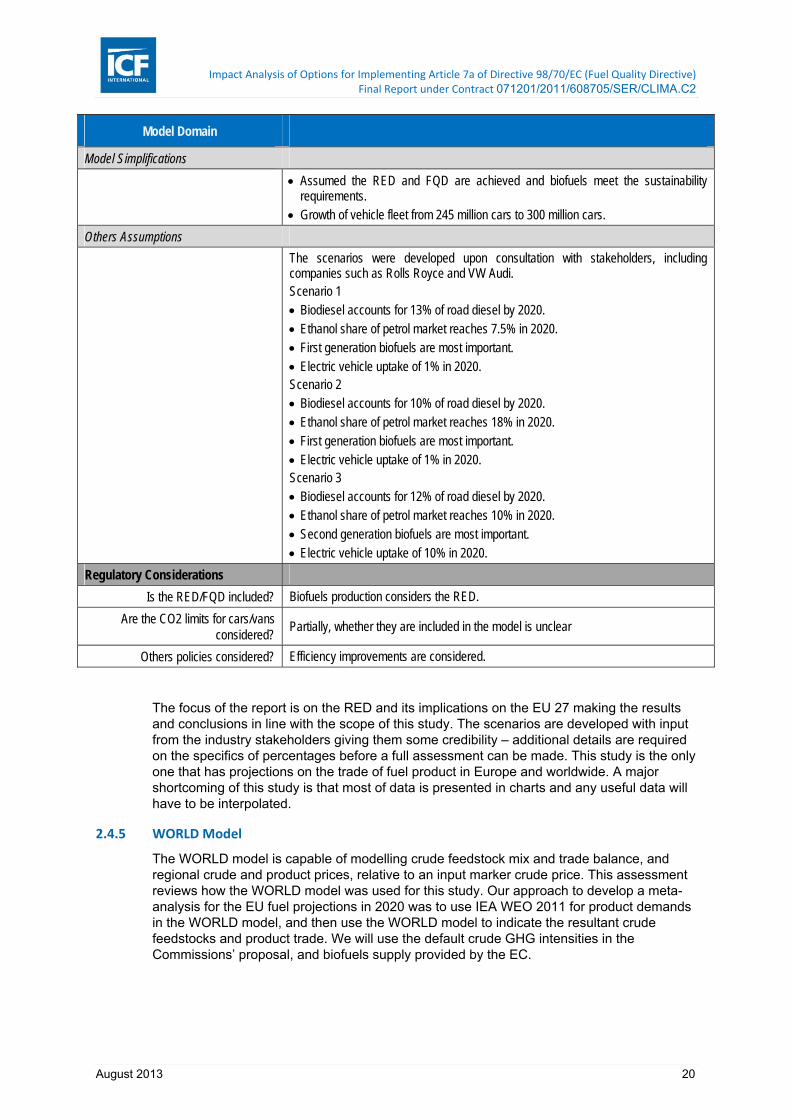
Impact Analysis of Options for Implementing Article 7a of Directive 98/70/EC (Fuel Quality Directive) Final Report under Contract 071201/2011/608705/SER/CLIMA.C2
August 2013 20
Model Domain
Model Simplifications
Assumed the RED and FQD are achieved and biofuels meet the sustainability requirements.
Growth of vehicle fleet from 245 million cars to 300 million cars.
Others Assumptions
The scenarios were developed upon consultation with stakeholders, including companies such as Rolls Royce and VW Audi. Scenario 1 Biodiesel accounts for 13% of road diesel by 2020. Ethanol share of petrol market reaches 7.5% in 2020. First generation biofuels are most important. Electric vehicle uptake of 1% in 2020. Scenario 2 Biodiesel accounts for 10% of road diesel by 2020. Ethanol share of petrol market reaches 18% in 2020. First generation biofuels are most important. Electric vehicle uptake of 1% in 2020. Scenario 3 Biodiesel accounts for 12% of road diesel by 2020. Ethanol share of petrol market reaches 10% in 2020. Second generation biofuels are most important. Electric vehicle uptake of 10% in 2020.
Regulatory Considerations
Is the RED/FQD included? Biofuels production considers the RED.
Are the CO2 limits for cars/vans considered?
Partially, whether they are included in the model is unclear
Others policies considered? Efficiency improvements are considered.
The focus of the report is on the RED and its implications on the EU 27 making the results and conclusions in line with the scope of this study. The scenarios are developed with input from the industry stakeholders giving them some credibility – additional details are required on the specifics of percentages before a full assessment can be made. This study is the only one that has projections on the trade of fuel product in Europe and worldwide. A major shortcoming of this study is that most of data is presented in charts and any useful data will have to be interpolated.
2.4.5 WORLD Model
The WORLD model is capable of modelling crude feedstock mix and trade balance, and regional crude and product prices, relative to an input marker crude price. This assessment reviews how the WORLD model was used for this study. Our approach to develop a meta-analysis for the EU fuel projections in 2020 was to use IEA WEO 2011 for product demands in the WORLD model, and then use the WORLD model to indicate the resultant crude feedstocks and product trade. We will use the default crude GHG intensities in the Commissions’ proposal, and biofuels supply provided by the EC.

Impact Analysis of Options for Implementing Article 7a of Directive 98/70/EC (Fuel Quality Directive) Final Report under Contract 071201/2011/608705/SER/CLIMA.C2
August 2013 21
Table 2.10 Detailed Assessment of WORLD Model
Model Domain
Level of Disaggregation
Are the EU 27 broken out? Yes, by applying a correction factor based on a ratio of fuel consumption for the EU-27 with respect to all of Europe
Is the data broken out for each member state?
No
Is the data broken out by individual refineries or refinery type?
No
Are the different feedstocks broken out?
Only for petroleum based fuels.
Are the different fuel types broken out? Some biofuels are included. Yes, all petroleum market fuels.
Are the different modes of transportation broken out?
Yes partially
Is the penetration of electric vehicles considered?
No.
Timescale
Range Projections for 2020 (Available range is to 2035).
Increments N/A
Year of actual data on which projections are based
2020 EU-27 and Worldwide Fuel Demand were based on IEA WEO 2011.
Other –
Data Quality
Is EUROSTAT used? No
What other sources are used? EIA IEA European Commission provided values for biofuels.
Do the GHG intensity values for biofuels match EC values in Annex 5 of
the RED for 2010?
No. Biofuel intensities were provided by the Commission. GHG intensities were modelled exogenous to WORLD.
Do the GHG intensity values for fossil fuels match Annex 1 of the amended
directive?
Yes. Fossil fuel intensities are from Annex 1. GHG intensities were modelled exogenous to WORLD
Transparency
Assumptions are delineated in section 2.5.1
Modelling Inputs
GDP Used IEA WEO 2011 projections
Population Used IEA WEO 2011 projections
Other Exogenous Used IEA WEO 2011 projections for energy demand. Price of crude from IEA WEO 2011.
Technical Considerations
Model Simplifications
Assumed all biofuel supply, per the data supplied by the EC, was consumed in EU. No additional biofuels were allowed in the model.
Others Assumptions

Impact Analysis of Options for Implementing Article 7a of Directive 98/70/EC (Fuel Quality Directive) Final Report under Contract 071201/2011/608705/SER/CLIMA.C2
August 2013 22
Model Domain
Regulatory Considerations
Is the RED/FQD included? No.
Are the CO2 limits for cars/vans considered?
Yes, based on IEA WEO 2011.
Others policies considered? Yes based on IEA WEO 2011.
2.4.6 Overall Comments
It is evident that not every source contains all of the key parameters. For example, the WEO 2011 and IEO 2011 are more globally-focused with data for world liquids demand, GDP growth, and population. It should be noted that Wood Mackenzie’s demand is for the year 2013 not 2020. Three of the five reports forecast European liquids demand. The WORLD model uses the IEA WEO 2011 forecast for demand in 2020. The WEO did not provide a fuel specific forecast of European liquids demand under the Current Policy Scenario. For the average annual percent change of the world GDP, the range among the data sources was 3.4 to 4.2 percent. Average annual percent change values for the world population ranged from 0.9 to 4.2 percent. The 2020 crude marker price in the WEO 2011 and IEO 2011 are $118/bbl and $108/bbl respectively, whilst the Wood Mackenzie source had a lower crude price of $89/bbl. The WORLD model uses the IEA WEO 2011 crude price in 2020.
2.5 2020 Baseline Fuel Demand Projections
As a result of the literature review, it was determined that a meta-analysis forecast will use the IEA WEO 2011 Current Policies Scenario for the 2020 baseline fuel demand and crude marker price. However the WEO 2011 does not provide EU27 specific crude trade and balance. The WORLD model will be used for indication of the crude feedstocks and product trade. ICF did not conduct a new fuel demand forecast such as assessing the changes in economic growth, population growth, energy prices, CO2 prices, nor changes in energy technologies. In addition the Commission provided the 2020 biofuel quantities and their GHG intensities as well as the assumed carbon price.
Key European country groupings used in this report:
■ EU27 countries: Austria, Belgium, Bulgaria, Cyprus, Czech Republic, Denmark, Estonia, Finland, France, Germany, Greece, Hungary, Ireland, Italy, Latvia, Lithuania, Luxembourg, Malta, Netherlands, Poland, Portugal, Romania, Slovak Republic, Slovenia, Spain, Sweden, United Kingdom.
■ WORLD model European countries: Austria, Belgium, Denmark, Finland, France, Germany, Iceland, Ireland, Luxembourg, Netherlands, Norway, Sweden, Switzerland, United Kingdom, Greece, Italy, Portugal, Spain, Turkey, Albania, Bulgaria, Czech Republic, Hungary, Poland, Romania, Slovak Republic, Former Yugoslavia.
2.5.1 Assumptions for the 2020 Baseline Forecast Model
This section outlines the meta analysis and calculations ICF carried out to develop the baseline fuel demand forecast in 2020. Below describes the step by step procedure for development of the baseline fuel and emission projections.
a. EU ETS. It was assumed that EU refineries pay the full cost of their CO2 emissions in 2020.
The amount of allowances that a refinery will get is, in simple terms:
Allowances = benchmark CO2 emissions intensity x historic production x allocation factor

Impact Analysis of Options for Implementing Article 7a of Directive 98/70/EC (Fuel Quality Directive) Final Report under Contract 071201/2011/608705/SER/CLIMA.C2
August 2013 23
Refining is defined as an activity exposed to carbon leakage, and so has an allocation factor of ‘1’ out to 2020 (in contrast to unexposed activities for whom the allocation factor gradually declines to 0.3).
The benchmark was set at the average of the top decile of EU performance; so that if a refinery is at this level of performance and produced the same volume as its historic production then it would get all its allowances free. However the level of free allowances does not depend upon how much is produced in the current period; they are just based on historic performance. So there is nothing about the free allocation amount that the refinery can change.
This means that the refinery has to buy additional allowances for every extra unit of emissions it produces. From an economic perspective this means that, assuming that emissions are proportional to output, then it is appropriate to model refinery behaviour as if they did face the full CO2 cost with no free allocation. The fact that emissions are lump-sum (sometimes called grandfathering) means that we should model them as facing the full marginal cost of the CO2 price.
The price provided by the Commission for the EU ETS carbon price is €16.5/ tCO2e.
b. The WORLD model used the IEA WEO 2011 crude price of $118/bbl in 2020
c. ICF included the exact amount of MS biofuels provided by the EC. Biofuel imports were not allowed.
d. The biofuel quantities may also result in diesel and petrol exceeding the B7 and E10 volume percent blend walls. There are significant biofuel blend wall limitations for logistics infrastructure and vehicles that are unresolved. However this forecast does not analyse the impact of these limitations. In the EU today, vehicles are E10 (from model year (MY) 2005) and B7 compatible. The US Environmental Protection Agency (USEPA) approved use of E15, for use in MY2007 and newer light-duty motor vehicles. However the EPA is being challenged in court by the Alliance of Automobile Manufacturers, Global Automakers, the Grocery Manufacturers Association, the oil industry and other groups claiming that a new fuel with a higher blend of ethanol could damage engines. Additionally, biodiesel has been used as a diesel blending component at levels up to 20% by volume.6 Compatibility of vehicles with higher biofuel blends are still to be proven and will require time, testing and investment. There are also questions regarding sustainability, pace of development, and imports of biofuels.
e. The PJ demand for EU-27 Road Transport Sector was updated using the 2012 IEA Midterm report published on Oct. 12, 2012. ICF used a meta-analysis method by using the IEA WEO 2011 for the year 2020 petroleum demand forecast.
f. ICF did not model compliance with the FQD in this 2020 baseline fuel projection forecast. In other words, the model was run as if the FQD does not exist.
g. Therefore the baseline forecast volumes of petroleum products, crude imports, and trade in the year 2020 were as if the FQD does not exist.
h. In Task 1.2 the GHG intensities were calculated with the resultant 2020 baseline volumes of fossil-origin fuels using the Commission’s Proposed crude feedstock intensities for conventional, bitumen, oil shale, etc., e.g.:
– Conventional diesel 89.1 gCO2e/MJ GHG intensity – Natural Bitumen diesel 108.5 gCO2e/MJ – Oil shale diesel 133.7 gCO2e/MJ
together with intensities for biofuels (provided by the EC) for bio-origin fuels. This may result in 2020 with a EU27 GHG intensity greater than 83 gCO2e/MJ.
i. ICF calculated the GHG intensity with double counting of 2G biofuels.
6 NREL, Impacts of Biodiesel Fuel Blends Oil Dilution on Light-Duty Diesel Engine Operation, June 2009, http://www.nrel.gov/docs/fy09osti/44833.pdf

Impact Analysis of Options for Implementing Article 7a of Directive 98/70/EC (Fuel Quality Directive) Final Report under Contract 071201/2011/608705/SER/CLIMA.C2
August 2013 24
2.5.2 Meta‐Analysis Forecast Begins with Data from IEA WEO 2011
The IEA WEO 2011 Current Policies Scenario, IEA 2012 Midterm Report, and IEA 2011 Midterm Report include fuel projections for petrol, diesel, LPG, kerosene, naphtha, residual fuels, and other products. It should be noted that the IEA forecasts include demand across all sectors, not just the transport sector7. The five fuels / energy types applicable to the FQD are petrol, diesel, LPG, CNG, and electricity.
ICF determined to use the 2011 WEO as the basis of the 2020 demand forecast. To evaluate effects on European crude trade and fuel trade, it is necessary that the fuel projection account for more than just the 5 FQD fuels and that the fuel projections include all sectors, not just road transport. To that end, the 2011 World Energy Outlook, in combination with the IEA 2012 Midterm Report, the IEA 2011 Midterm Report, SULTAN, and historical IEA data for 2009, were used to provide suitable demand projections for the FQD fuels as well as allow for the evaluation of trade impacts.
2.5.3 Apportion Total Fuel Demand from IEA Midterm Report to the Road Transport Sector
The WEO does not provide a breakout of specific fuels such as petrol and diesel. However ICF was able to obtain from IEA the specific fuels breakout of the 2012 IEA Midterm report, which has projections to 2017. Therefore ICF applied the Midterm 2017 fuels breakout to the WEO 2020 forecast.
The data from the IEA 2012 Midterm Report contained fuel projections which did not distinguish across sectors. Therefore, it was necessary to apportion total fuel demand to the road transport sector. ICF assumed that all petrol and diesel demand was attributable to the transport sector. The diesel in the 2012 Midterm Report includes road transport, NRMM and any diesel if used in inland waterways. We assume there is partial use of diesel in international or coastal maritime movements to reflect the Baltic and North Sea ECAs; also, the EU rule passed in September 2012 that requires 0.5% sulphur fuel to be consumed in all EU non-ECA areas by 2020 was incorporated. The gasoil in the 2012 Midterm Report is for household heating and industrial appliances, and not for transport. Note that there is a separate residual fuel category which covers the majority of maritime fuel usage. However, the same could not be reasonably assumed for LPG. As such, historical data from IEA was used to develop a ratio of LPG used in road transport and total LPG demand. This ratio was then applied to the data from the IEA Midterm Report. The inherent assumption being that the proportion of LPG used in the road transport sector will remain constant. Table 2.11, below, summarizes the underlying data and development of the ratio.
Table 2.11 IEA 2009 Historical Fuel Consumption Data – Road Transport and Total
Fuel Road Transport Sector
(1000 tonnes) Total Consumption (1000
tonnes) Mass Ratio
LPG 4,729 23,231 20.36%
2.5.4 Scaled Projections to 2020
To breakout the WEO’s 2020 projections, a ratio of each of the fuels to the total demand in the Midterm for 2017 was used. Table 2.12 summarizes the ratios of each fuel to the total liquids demand.
7 The FQD applies to road transport, non-road mobile machinery (including inland waterway vessels), agricultural or forestry tractor or recreational craft.

Impact Analysis of Options for Implementing Article 7a of Directive 98/70/EC (Fuel Quality Directive) Final Report under Contract 071201/2011/608705/SER/CLIMA.C2
August 2013 25
Table 2.12 Ratio of Specific Fuel Demand to Total Demand in 2017 Midterm
Fuel Volume Ratio
Petrol 13.9%
Diesel 31.7%
Gasoil 12.3%
LPG 6.1%
Kerosene 9.1%
Ship Fuel 8.8%
A ratio of OECD Europe fuel demand to EU-27 fuel demand was determined based on Total Petroleum Demand in 2017 from IEA’s 2011 Midterm Report (resulting value of 1.062)8. Combining the ratios in Table 2.12, ratio of OECD Europe to EU-27 demand, and the total liquids demand in OECD Europe from the WEO, a projection of fuel demand in the EU-27 in 2020 was developed. Table 2.13 summarizes the resulting projection. The ratios from 2017 in Table 2.12 were applied to 2020.
Table 2.13 2020 Scaled IEA Fuel Projections for EU‐27
Fuel 2020
(1000 bpd) 2020 (PJ)
Petrol 1,593 2,958
Diesel (10 ppm sulphur max) 3,633 7,590
Gasoil (50 ppm sulphur max) 1,411 2,947
Electricity N/A N/A
LPG 695 1,020
CNG N/A N/A
Kerosene 1,046 2,003
Ship Fuel 1,005 2,333
TOTAL 9,383 18,851
Data on electricity and CNG could not be provided by IEA in the timescales of this study
Table 2.14, below, summarizes the 2020 projections for the road transport sector based on the IEA 2011 WEO with the product breakouts based on the Midterm Report in year 2017. This includes adjusting the diesel and LPG to that only within the road transport sector.
Table 2.14 2020 Scaled IEA Fuel Projections for EU‐27 Transport Sector
Fuel 2020
(1000 bpd) 2020 (PJ)
Petrol 1,593 2,958
Diesel 3,633 7,590
Electricity N/A N/A
8 The IEA 2011 Midterm Report was used to develop this ratio because the data from the IEA 2012 Midterm Report did not include non EU-27 countries.

Impact Analysis of Options for Implementing Article 7a of Directive 98/70/EC (Fuel Quality Directive) Final Report under Contract 071201/2011/608705/SER/CLIMA.C2
August 2013 26
LPG 141 208
CNG N/A N/A
Kerosene 0 0
Ship Fuel 0 0
TOTAL 5,367 10,756
The diesel in IEA’s 2012 Midterm Report includes both on-road diesel and off-road diesel (including non-road mobile machinery and inland waterway vessels). The WORLD model also models this combined diesel demand and models it for 2020 at 10 ppm maximum sulphur specification. Therefore the off-road diesel is not a separate input to the WORLD model. However, to break out the diesel into the two subcategories, on-road diesel and off-road diesel, the 2020 forecast in the JEC report titled “EU renewable energy targets in 2020: Analysis of scenarios for transport” was used. From the JEC report, proportions of on-road diesel and off-road diesel compared to total diesel could be generated. Table 2.15 summarizes the resulting ratios.
Table 2.15 2020 On‐Road Diesel and Off‐Road Diesel Ratios from JEC Report
Fuel % of TOTAL DIESEL
On Road Diesel 87.7%
Off Road Diesel 12.3%
Table 2.16, below, summarizes the fuel projections in Table 2.14 with the diesel now differentiated between on-road and off-road.
Table 2.16 2020 Scaled IEA Fuel Projections for EU‐27 Transport Sector
Fuel 2020
(1000 bpd) 2020 (PJ)
Petrol 1,593 2,958
Diesel 3,633 7,590
Diesel On Road 3,187 6,659
Diesel Off Road 446 931
Electricity N/A N/A
LPG 141 208
CNG N/A N/A
Kerosene 0 0
Ship Fuel 0 0
TOTAL 5,367 10,756
2.5.5 Incorporate Electricity and CNG Demand
The IEA 2012 Midterm Report estimates of electricity and CNG demand in the road transport sector were not available. As such, SULTAN was selected as the best available estimate for demand for CNG, and the EC provided the electricity demand in the road transport sector. Table 2.17 illustrates the combination of the road transport projections from Table 2.16 with SULTAN’s projections for CNG demand and the EC provided electricity demand in the road transport sector in 2020 for the EU-27.

Impact Analysis of Options for Implementing Article 7a of Directive 98/70/EC (Fuel Quality Directive) Final Report under Contract 071201/2011/608705/SER/CLIMA.C2
August 2013 27
Table 2.17 2020 Fuel Projections for EU‐27 Road Transport Sector
Fuel 2020
(1000 bpd) 2020 (PJ)
Petrol 1,593 2,958
Diesel (10 ppm Sulphur Max) 3,633 7,590
Diesel On Road 3,187 6,659
Diesel Off Road 446 931
Electricity N/A 86.8
LPG 141 208
CNG 84 44
Kerosene 0 0
Ship Fuel 0 0
TOTAL 5,451 10,886
In addition we analysed IEA’s scaled forecast with historical data. Historical data for petrol and diesel consumption from EUROSTAT for 2006 through 2010 were used, and scaled projections from the WEO. The historical and projection data were plotted from beginning in 2010 to 2020 in Table 2.18 and Table 2.19, below. The result verifies that the projections are consistent with historical data.
Table 2.18 Petrol Demand in EU‐27, 2006 – 2020
0
500
1,000
1,500
2,000
2,500
3,000
3,500
4,000
4,500
5,000
2004 2006 2008 2010 2012 2014 2016 2018 2020
EU‐27 Petrol (PJ)
IEA Scaled Projection
EUROSTAT Historical

Impact Analysis of Options for Implementing Article 7a of Directive 98/70/EC (Fuel Quality Directive) Final Report under Contract 071201/2011/608705/SER/CLIMA.C2
August 2013 28
Table 2.19 Diesel Demand in EU‐27, 2006 – 2020
2.5.6 EC Supply of Biofuels
The EC provided ICF with an estimate of biofuel supply broken down by feedstock in 2020. The estimate was in units of million tonnes of oil equivalent (Mtoe). Based on discussions with the EC, these values represented the estimated supply of biofuels from the EU Member States. Table 2.20, below, summarizes the biofuel supply estimates provided by the EC.
Table 2.20 2020 EU‐27 Road and NRMM Biofuel Supply Projections
Biofuel Feedstock Baseline 2020 (Mtoe) Baseline 2020 (PJ)
Corn (maize) 0.69 28.59
Sugar beet 0.96 40.20
Sugar cane 2.47 103.11
Wheat Process fuel not specified 0.36 14.86
Wheat Natural gas as process fuel in CHP plant 0.36 14.86
Wheat Straw as process fuel in CHP plant 0.36 14.86
2G ethanol - land using 0.23 9.70
2G ethanol - non-land using 0.23 9.70
2G biodiesel - land using 0.37 15.34
2G biodiesel - non-land using 0.37 15.34
Waste 1st. Gen. diesel 0.74 30.67
Palm oil 1.96 82.18
Palm oil with methane capture 1.96 82.05
Rapeseed 9.20 385.29
Soybean 2.50 104.98
Sunflower 0.94 39.66
TOTAL 23.71 991.4
Source: Provided by the EC.
0
2,000
4,000
6,000
8,000
10,000
12,000
2004 2006 2008 2010 2012 2014 2016 2018 2020
EU‐27 Diesel (PJ)
IEA ScaledProjection
EUROSTATHistorical

Impact Analysis of Options for Implementing Article 7a of Directive 98/70/EC (Fuel Quality Directive) Final Report under Contract 071201/2011/608705/SER/CLIMA.C2
August 2013 29
2.5.7 2020 Baseline Demand Scenario Combination
The petroleum based fuel demand from the combination of the WEO and IEA Midterm Reports, as described above, for road and non-road mobile machinery was combined with biofuel supply provided by the EC. ICF set the total energy demand from road vehicles and non-road mobile machinery to be 10,886 PJ, per the analysis above. Then, based on the biofuel supply provided by the EC, ICF calculated the amount of petroleum based fuels that would be displaced by these biofuels9. As a result, an estimate of the total demand of fuel for both biofuels and petroleum based fuels was developed while maintaining total energy demand from this sector at 10,886 PJ.
2.6 Feedstock and Product Projections
2.6.1 Introduction to the WORLD Model
The WORLD linear program (LP) model marries top down oil price/supply/demand outlooks, such as those that are developed by the IEA, EIA, OPEC and others, with bottom up detail: around 200 crude oils, non-crudes breakdown (NGL’s, biofuels, GTL/CTL etc.), data on every refinery worldwide with aggregation into regional or sub-regional groups, multiple products and product quality detail/specifications, detailed marine, pipeline and minor modes transport representation, refining sector GHG emissions, projects, investments. This combination is capable of modelling any current or future horizon out to (current model) 2035, simulating how the industry is likely to operate and react under any given scenario and capturing the interactions and competition inherent in the global downstream. The World petroleum industry is technically complex, has the economic attributes of a co-product industry and its different aspects and regions are highly inter-related. The industry’s inter-connections and market interactions are global and contain considerable ability to adjust to changed circumstances. The industry is faced today by major challenges presented by environmental, product quality, conservation, substitution, supply/demand and technology/cost developments. The WORLD model is designed to bring all of the key elements of the world petroleum/”liquids” industry together into one simulation tool, with the specific goal that it be able to realistically address developments that are departures from the status quo and do so across a wide range of time-frames. The model formulation aggregates the world into 22 regions. The WORLD model is capable of modelling regional refining projects, capacity additions and investments, crude feedstock mix and crude and product trade balances, and regional crude and product prices, relative to an input marker crude price.
2.6.2 Key drivers of Product Trade in WORLD Model
This section summarizes some of the key drivers of fuel product imports into the EU from the rest of the world in the WORLD model, with a particular emphasis on imports of ultra-low-sulphur diesel with a maximum of 10 ppm of sulphur (ULSD or 10 ppm diesel).
2.6.2.1 Key features of model operation in relation to fuel product imports into the EU
Projected demands by product category and grade (including ULS and other diesel grades) are exogenous inputs to the WORLD model, driven by a combination within the WORLD model of the “top down” scenario for high level demands by region with “bottom up” detail on product grades and qualities. Production of fuels (including 10ppm diesel) in each world region, and shipping from region to region, including export to the EU, are calculated endogenously in the WORLD model.
Product production and inter-regional flows, together with other activities such as crude flows etc. result from the simulations in the model of the operations, technology and
9 It is likely that the increased demand for biofuels, along with developments in the petroleum refining market, would induce price dynamics that are not taken into account in this calculation. If the study reveals that the impact of the directive is sensitive to the share of imported biofuels and their source, then further analysis will be undertaken in later phases.

Impact Analysis of Options for Implementing Article 7a of Directive 98/70/EC (Fuel Quality Directive) Final Report under Contract 071201/2011/608705/SER/CLIMA.C2
August 2013 30
economics of the world petroleum / liquids industry, using all the available options (crude shipping, refinery processing, refinery investment, blending, intermediates and product shipping) to satisfy product demand feasibly and optimally (i.e. at minimum global cost); this while respecting all the constraints on the system, notably supply limits, shipping limits, process capacity and operational limits, product blending specifications, regional product demands, etc.
2.6.2.2 Model inputs
The following are the key exogenous inputs into the model. They are case-specific:
■ Energy prices
– Global oil price, input as the price of the marginal/marker crude
– Natural gas prices (major industrial user by region), coal price relationships (for fuel grade petroleum coke)
– Also prices for elemental sulphur and for methanol as a feedstock for MTBE production
– If applicable, GHG emissions costs, e.g. price per tonne of CO2 emitted by refineries in which there is a carbon regime in place.
■ Feedstocks
– Crude: production outlook including balance of future OPEC versus non-OPEC production; specific country crude production and mix. (Supply level of marker crude is allowed to float, those of all other crude oils exogenously determined and fixed)
– “Non-crudes”: supply by type, including NGL’s, biofuels, CTL’s, GTL’s (so e.g. a high biofuels supply case would be consistent with high substitution of petroleum products by alternative fuels). The CTL, in Germany, is based on historical volumes and is not broken out by projects.
■ Products
– Product demand: built up from underlying historical data and growth rates/projections.
– Product quality: evolution of petrol, distillates, kerosene, jet fuel, naphtha, marine and residual fuel quality standards / specifications by region, especially based on mandates for clean and reformulated fuels.
■ Product production
– Base refinery capacity
– Firm new projects, i.e. the subset of total announced projects that it is estimated will go ahead. (Generally, projects have to be already under construction or at advanced engineering stage to be included.)
– New capacity investment costs, including evolution of regional capital cost location factors for process unit investments depending on the effects of environmental legislation.
– New refining technologies: availability and costs.
■ Transport
– Inter-regional routes, modes, costs and capacities including:
Marine – tanker/major barge routes, typical associated tanker size/class, estimated freight rates based on WorldScale, import tariffs
Pipeline capacity limits), firm (or potential) pipeline projects and costs
Rail and selected other minor movements.

Impact Analysis of Options for Implementing Article 7a of Directive 98/70/EC (Fuel Quality Directive) Final Report under Contract 071201/2011/608705/SER/CLIMA.C2
August 2013 31
The base approach in the model is to not exogenously limit crude oil and product movements. There are certain exceptions. One is that selected crude oil movements are limited or trended based on geo-political considerations, e.g. no Iranian crude imports to USA, assumed steadily growing Venezuelan crude oil exports to China. Another important example is that of Russian product exports. For these, historically, “normal economics” have not always worked. Consequently, a semi-exogenous approach is used to set total product exports within a range (while allowing for endogenous flexibility within that range). In the base case, historical trends and data and commentary from the IEA were reviewed and potential 2020 FSU product exports were set within a range based on these inputs. Summary details of the values used for key input parameters and sources of data are given in Table 2.21 of this report.
Overall, the input data for the model covers thousands of data points, with hundreds of different information sources collected over 25 years and continuously researched and updated. There are some key starting points for the data (e.g. IEA medium term outlook, Oil and Gas Journal, WorldScale flat rates etc.). However data are also brought in from other sources as needed, including additional references, literature/industry press research, plus professional judgement.
2.6.2.3 Model outputs
Key outputs from the model include a combination of physical/activity and economic/pricing parameters:
■ Feedstocks / products
– Supply/demand balances, including global supply/demand volume and balance cross-checks
– Crude and product inter-regional movements
– Crude and product prices and differentials (relative to the marker crude price which is an input)
– Cracking / refining margins
– Total supply cost by region (product price * demand volume)
■ Refining / product production
– Regional refinery throughputs, utilisations, capacity additions by unit type and associated investments($)
– Refinery operations, feeds/modes on crude units and all major refining units, including upgrading, desulfurization, catalytic reforming
– Product blending (consistent with meeting input product quality specifications)
– Regional refinery CO2 emissions
■ Transport
– Pipeline and marine transport mode movement volumes / trade for crudes and products
– Utilizations /expansions on capacity-limited modes, notably pipelines
2.6.3 Summary of Premises for Model Run
Table 2.21 summarises key premises used for the WORLD Model case developed to establish a baseline for 2020.
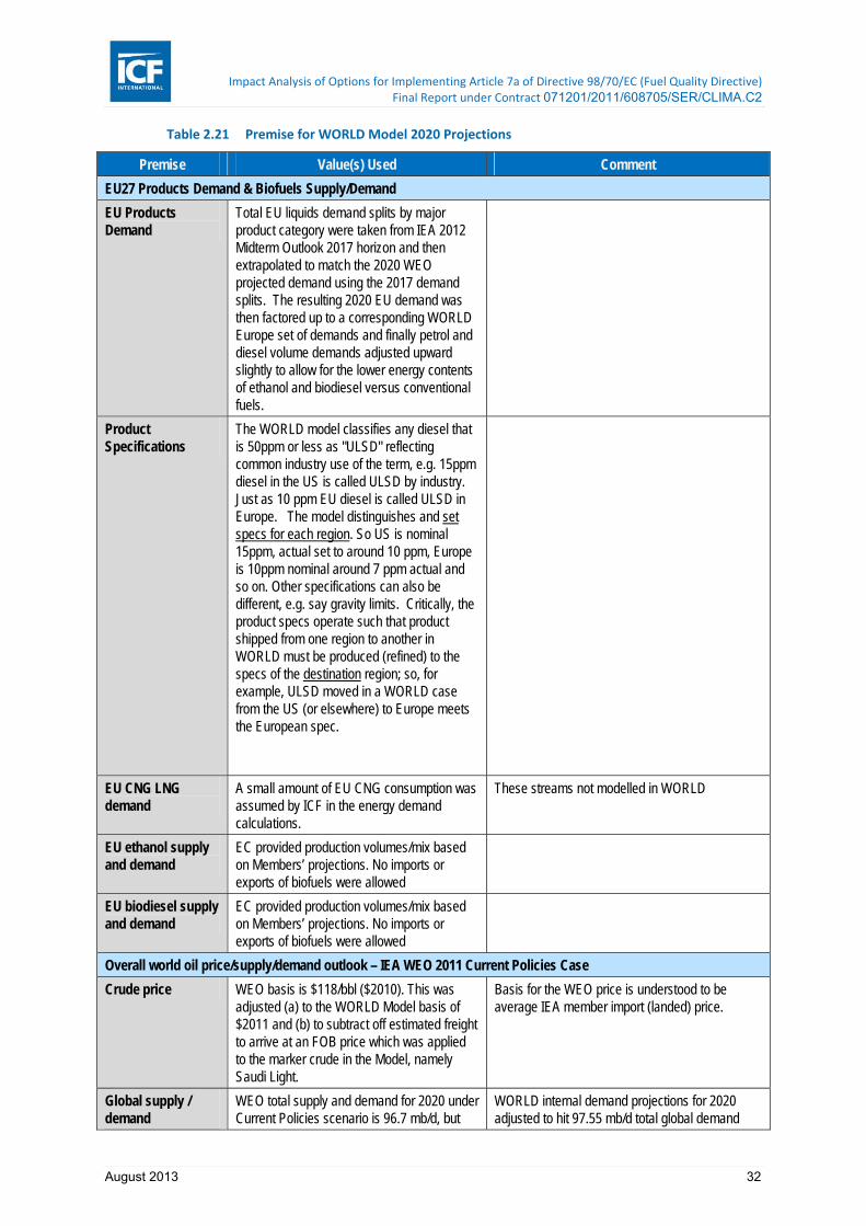
Impact Analysis of Options for Implementing Article 7a of Directive 98/70/EC (Fuel Quality Directive) Final Report under Contract 071201/2011/608705/SER/CLIMA.C2
August 2013 32
Table 2.21 Premise for WORLD Model 2020 Projections
Premise Value(s) Used Comment
EU27 Products Demand & Biofuels Supply/Demand
EU Products Demand
Total EU liquids demand splits by major product category were taken from IEA 2012 Midterm Outlook 2017 horizon and then extrapolated to match the 2020 WEO projected demand using the 2017 demand splits. The resulting 2020 EU demand was then factored up to a corresponding WORLD Europe set of demands and finally petrol and diesel volume demands adjusted upward slightly to allow for the lower energy contents of ethanol and biodiesel versus conventional fuels.
Product Specifications
The WORLD model classifies any diesel that is 50ppm or less as "ULSD" reflecting common industry use of the term, e.g. 15ppm diesel in the US is called ULSD by industry. Just as 10 ppm EU diesel is called ULSD in Europe. The model distinguishes and set specs for each region. So US is nominal 15ppm, actual set to around 10 ppm, Europe is 10ppm nominal around 7 ppm actual and so on. Other specifications can also be different, e.g. say gravity limits. Critically, the product specs operate such that product shipped from one region to another in WORLD must be produced (refined) to the specs of the destination region; so, for example, ULSD moved in a WORLD case from the US (or elsewhere) to Europe meets the European spec.
EU CNG LNG demand
A small amount of EU CNG consumption was assumed by ICF in the energy demand calculations.
These streams not modelled in WORLD
EU ethanol supply and demand
EC provided production volumes/mix based on Members’ projections. No imports or exports of biofuels were allowed
EU biodiesel supply and demand
EC provided production volumes/mix based on Members’ projections. No imports or exports of biofuels were allowed
Overall world oil price/supply/demand outlook – IEA WEO 2011 Current Policies Case
Crude price WEO basis is $118/bbl ($2010). This was adjusted (a) to the WORLD Model basis of $2011 and (b) to subtract off estimated freight to arrive at an FOB price which was applied to the marker crude in the Model, namely Saudi Light.
Basis for the WEO price is understood to be average IEA member import (landed) price.
Global supply / demand
WEO total supply and demand for 2020 under Current Policies scenario is 96.7 mb/d, but
WORLD internal demand projections for 2020 adjusted to hit 97.55 mb/d total global demand

Impact Analysis of Options for Implementing Article 7a of Directive 98/70/EC (Fuel Quality Directive) Final Report under Contract 071201/2011/608705/SER/CLIMA.C2
August 2013 33
Premise Value(s) Used Comment
with 2.1 mb/d of biofuels supply stated as barrels of equivalent petrol/diesel. Since WORLD works on volume barrels, the 2.1 mboe/d biofuels supply was adjusted to an estimated 2.95 mb/d (see below) and global volume supply and demand were each correspondingly adjusted, i.e. by +0.85 mb/d to 97.55 mb/d.
after first adjusting European demands to fit IEA-based projection
Global biofuels supply
IEA Current Policies projects 2.1 mb/d 2020 oil equivalent. EnSys estimated this equates to around 2.95 mb/d in volume terms and applied this total
EU ethanol and biodiesel production volumes were higher than in internal WORLD projection so other regions’ supply prorated down to accommodate the higher EU numbers and hit the IEA global target.
OPEC/non-OPEC supply
The data available in the WEO for 2020 Current Policies supply (Table 3.4) show OPEC and non-OPEC crude, NGL’s and non-conventionals but do not provide any breakdown of these. Consequently, EnSys adjusted (non-biofuels) supply to meet the same ratio of OPEC to non-OPEC supply as in the WEO. The adjustments were small.
Crudes supply Within WORLD, “top level” regional supply of oil liquids is taken from a third party projection, e.g. IEA or EIA, and then broken down to first subtract out non-crudes supplies (often these are split out in the projection). Total crude supply for a given region is then split out between the relevant crude grades based on extensive in-house research and data on current and projected crude production by main crude grade. This process includes both conventional and non-conventional crude oils. In any WORLD case, production levels are for all individual crude grades except for the marker/marginal crude (generally Saudi Light is used). An input price is assigned to the marker crude based on the projection for world crude price.
Non-crudes supplies for all except methanol (for MTBE feed) and natural gas (for hydrogen plant feedstock and refinery fuel) are also projected and fixed in any given case. (Prices are assigned to methanol and natural gas.) Product demands are worked up in a similar way and are fixed for all except the refinery by-products of sulphur and fuel grade petroleum coke (which are given prices and allowed to float). The effect is that, within any one case, the prices of every crude except the marker and of every non-crude and product are outputs from the case – not inputs.
Refinery Data
Base capacity, projects and closures
Internal WORLD data used. European Union projects were checked and reconciled against data supplied by EC.
Note, in current WORLD model, total refining capacity is aggregated in each of the 3 European Model regions.
Process technology and economics
Internal WORLD data
Product blending and quality / specifications
Internal WORLD data and projections taking account of actual blended qualities versus specifications. Progressive trend to LS/ULS standards in non-OECD regions
Marine fuels MARPOL Annex VI 0.1%S for ECA’s in 2015. No new ECA’s by 2020 beyond Europe (2) and Canada/USA. In line with IEA assessment, date for implementation of 0.5% sulphur global standard put back to 2025.
Effect of shifting the assessed implementation date for global 0.5% fuel to 2025 was to cause a shift in all world regions back from marine distillate to IFO – versus a 2020 implementation assumption – partially offset in Europe by an

Impact Analysis of Options for Implementing Article 7a of Directive 98/70/EC (Fuel Quality Directive) Final Report under Contract 071201/2011/608705/SER/CLIMA.C2
August 2013 34
Premise Value(s) Used Comment
However, EU rule passed in September 2012 that requires 0.5% sulphur fuel to be consumed in all EU non-ECA areas by 2020 was incorporated.
assumed impact of the EU 0.5% 2020 standard in shifting some IFO consumed in (mainly southern and eastern i.e. non-ECA) Europe to marine distillate.
EU petrol and diesel specifications
Internal WORLD data checked to ensure consistency against -supplied data, including for ethanol-in-petrol vapour pressure waiver
EU Carbon regime / cost
EU ETS €16.5/ tCO2e assumed for carbon price. Assumed in modelling that EU refiners pay carbon price on 100% of their CO2 emissions
Price based on reference scenarios utilised for assessments underpinning the results presented in the Commission's communications "Energy Roadmap 2050"10 and "Roadmap for Moving to a Competitive Low-Carbon Economy in 2050"11Euro/dollar exchange rate 1.25 hence dollar cost of $20.60 /tCO2E. Note, an energy efficiency trend was allowed for in the case but the option to “buy” more energy efficient means to generate steam/power and/or to consume fuel/steam/power more efficiently would have to be built in to the model
Other carbon regimes
No other major regimes assumed except for California LCFS (which is being challenged in court) and then only to extent of blocking WCSB oil sands crudes from being processed in the state
Logistics & Trade
Marine routes, tanker types, freight rates
Extensive movements for crudes and products basis internal WORLD data based on WorldScale. Panama Canal expansion by 2015
Movements generally not constrained other than where there are clear known situations that force or prevent specific movements e.g. for geo-political reasons or where crudes are known to be refined locally. Examples that are actively incorporated within the WORLD Model include: projected gradually increasing volumes of Venezuelan crude shipped to China to reflect geo-political ties and deals between the two countries, no Iranian crude to USA, requirements that selected crude oils in oil-producing countries be refined locally based on knowledge of the refineries there.
Pipelines Inter-regional pipelines, basis WORLD internal data/projections, including: USA/Canada pipelines and rail: TransMountain expansion to 750,000 b/d assumed by 2020 but not Northern Gateway (affects volumes of WCSB crudes moving to BC and Asia versus into US/eastern Canada), total WCSB capacity to Gulf Coast over 1.7 million b/d pipeline (Seaway, KXL, Pegasus) plus rail at 200,000 b/d. Total capacity 1.9 million b/d. Other crudes also utilize this
10 SEC(2011) 1565 p. 2. 11 SEC(2011) 288 p. 112

Impact Analysis of Options for Implementing Article 7a of Directive 98/70/EC (Fuel Quality Directive) Final Report under Contract 071201/2011/608705/SER/CLIMA.C2
August 2013 35
Premise Value(s) Used Comment
capacity. ESPO pipeline capacity to Komsomolsk / Asia 1.5 million b/d
Notes:
1. WORLD marries “top down” projections as from the IEA, EIA, OPEC or others with “bottom up” detail. The details in the WORLD Model used for this case have been built up from multiple sources (and 25 years of experience with the Model) including recent studies with and for the U.S. Departments of Energy and State, EPA, American Petroleum Institute, International Maritime Organisation, World Bank and OPEC Secretariat, with whom EnSys undertakes a joint annual study of the global downstream outlook that is now published as part of the annual OPEC World Oil Outlook.
2.6.4 Model Output and Results
The results presented in this report on feedstock and product projections should be regarded as indicative rather than definitive. The key results and findings are set out in the sections below.
■ Actual 2011 crude throughputs for WORLD Model Europe 3 regions – 13.1 mbd (with demand approx. 15.3 mb/d)
■ Compares to 2020 revised base case projection of 10.2 mbd throughput for WORLD Model Europe based on estimated 2020 demand from IEA projections of 13.04 mbd (which equates to 12.7 mbd for the EU27 including CNG and LNG)
■ Thus, versus 2011, projected demand drops by nearly 2.3 mbd but projected refinery throughput by 2.9 mbd, i.e. refinery throughput drops by more than demand. This reduction is dependent on and sensitive to competition from other regions, has an underlying assumption that product exports from the FSU will continue to slowly grow, and incorporates assumed carbon costs of €16.5/ tCO2e on European refinery operations which will tend to cut European refinery throughputs.
■ With World Model Europe projected base capacity (including firm projects and net of recent closures) of 16.4 mbd and projected 2020 throughput of 10.2 mbd, associated utilisation is 62%. At this throughput, gaining a long term sustainable utilisation of 85% would imply a further 4.4 mbd of closures across Europe; this in addition to the 1.6 mbd of recent closures allowed for in the base capacity. Again, this outlook is sensitive to assumptions. (Note – no additional refineries were closed beyond the ones listed in Table 2.25.)
■ WORLD definition of FSU has 9.1 mbd of base capacity including firm projects. Projected 2020 crude throughput is 6.45 mbd hence utilization is 71%
■ Among major secondary units, only hydro-crackers are projected as having sustainable utilisations (consistent with the implication from the Model case that substantial additional refinery closures could be necessary by 2020).
■ No refinery capacity additions (crude capacity or secondary processing) beyond allowed for projects are projected for Europe by 2020. While some minor revamps and debottlenecks may indeed occur, this overall picture is not surprising given the combination of across the board projected demand decline combined with higher operating costs through assumed payments for carbon emissions.
■ Total product exports from WORLD Model Europe regions are projected at 1.7 mbd and imports at 2.4 mbd. Associated projected petrol exports are just over 1 mbd and net distillate imports (jet/kero + gasoil/diesel) just under 1 mbd. The primary destinations for petrol exports are projected to be USA/Canada and Africa and the main sources of distillates imports the FSU and USA/Canada. The demand projection for the USA used in the 2020 case had demand levels only slightly below those for 2011. In its 2013 AEO released in December 2012, the EIA has revised downward its outlook for US demand.

Impact Analysis of Options for Implementing Article 7a of Directive 98/70/EC (Fuel Quality Directive) Final Report under Contract 071201/2011/608705/SER/CLIMA.C2
August 2013 36
As a result, product production in and flows into the U.S. East Coast region – PADD1 – were fairly similar in the 2020 Model results as were actual levels for 2011. However, the Model case did have European petrol exports moving into eastern Canada which bear further inspection as premises may have led to them being on the high side.
■ Imports of GTL distillates are projected to be modest. As the primary producer, the Middle East is projected to either blend GTL diesel into blends at local refineries (potentially for export) and to send its actual GTL exports predominantly to Asia. These projections are subject to uncertainty based, inter alia, on such factors as corporate ownership interests. Majority of modelled GTL imports will come from Africa, and small amounts from Latin America.
■ Distillates are projected to continue to maintain a significant price premium over petrol and thus 2-1-1 crack spreads well ahead of 3-2-1.
■ 2020 European crude slate is projected at 51% sweet, of which the sweet grades are predominantly North and West African. This appears plausible versus a recent historical mix of round 50/50 and given the effect of carbon costs of €16.5/ tCO2e in tending to disadvantage heavier / higher sulphur crudes which need more processing. Other main crude import sources are projected as FSU/Caspian, Middle East and Latin America.
■ 2020 World Model Europe crude slate includes 6,700 b/d of Estonian oil shale. Estonian shale oil volumes are based on research by ICF and Ensys, the historical production is kept flat.
■ The 2020 base case has the ESPO system in full operation which increases Russian crude exports to Asia. Projected ESPO 2020 capacity is 1.5 mbd with total throughput in the case running at 1.3 mbd of which around 0.4 mbd runs on the spur into China and the rest out to the Pacific.
■ All crude oil imports shown are conventional with the potential exception (depending on classification) of Venezuelan synthetic crude volumes. These volumes may well be simply an artefact of the case in the sense of Model selection between Venezuelan heavy conventional versus Orinoco-derived crudes. It should be remembered that not all heavy crudes coming into a region will be upgraded. One reason for demand for heavy grades from Venezuela and elsewhere is to satisfy demand for asphalt.
■ All product imports modelled are derived from conventional feedstocks with the exception of US diesel arriving from the Gulf coast (USGC), GTL arriving from Africa and Latin America.
■ Canadian oil sands crudes are not predicted to come across to Europe, especially pre 2020. The premises allow for a number of major pipeline projects to go ahead (Trans Mountain expansion, Seaway reversal and expansion, Keystone XL, also non-trivial rail movements) that will add substantial capacity to move Western Canadian Sedimentary Basin (WCSB) crudes west and to Asia as well as to US coastal markets, notably the Gulf Coast. If these projects do not all go ahead, we believe alternatives will develop. Rail is expanding rapidly in the US, currently taking mainly Bakken crudes to markets on the West, Gulf and East coasts in volume. In addition, rail shipment of WCSB crudes is now starting to take off to destinations in the US and also Eastern Canada. (Shipping oil sands bitumen by rail is more competitive with pipeline as the bitumen can be shipped with less or no diluent (in insulated rail cars) and because pipeline tariffs are higher for shipping DilBit versus light crude.) Further, Enbridge and TransCanada are considering pipeline expansions / conversions to take WCSB crudes in larger volumes to Canadian refineries in Ontario, Quebec and the Maritimes. We believe these factors will keep the WCSB oil sands streams within the USA and Canada at least through 2020. What happens after 2020 will depend on how pipeline and rail capacity has evolved, including whether and when the Trans Mountain expansion and the Northern Gateway projects go ahead. A lack of capacity from WCSB to the British Columbia coast and thence Asia will put pressure on bringing the WCSB crudes south and east. One possibility that would tie in with existing projects would be to reverse the Portland to Montreal pipeline once Enbridge has completed reversal of its Line 9 so that it (once again) runs east from

Impact Analysis of Options for Implementing Article 7a of Directive 98/70/EC (Fuel Quality Directive) Final Report under Contract 071201/2011/608705/SER/CLIMA.C2
August 2013 37
Sarnia to Montreal. However, currently, it appears that much of the planned available capacity on Line 9 has been committed for refineries within eastern Canada, leaving limited or even no apparent potential for onward exports from Portland Maine. Even if such volumes were available, destinations such as Jamnagar in India could compete with European heavy upgrading (or asphalt) refineries for the available volumes. Again, at least before 2020, we see it as more likely that US Lower 48 crudes could start to be exported (beyond Canada), given the relevant export permits, than WCSB crudes for which a substantial ready market exists on the US Gulf Coast.
■ In the base case, Canadian oil sands streams do, because of the pipeline expansions, flow in volume (approximately 0.85 mbd) to US Gulf Coast refineries and those refineries do in turn export distillate to Europe. However, the volumes moved to Europe are small relative to the region’s total output which is also used domestically and for exports to other regions, notably Latin America12. In the 2020 base case, Venezuelan Orinoco syncrude is projected as flowing to the USGC (over 0.5 mbd). Depending on the classification by the EU of those streams, the same issue could apply as with production and export of distillate from oil sands crudes. Again, at the volumes projected, Gulf Coast refiners would appear to have enough options to ensure that distillates derived from Venezuelan syncrude processing would likely not move to Europe, especially if there were a higher carbon cost penalty attached.
2.6.5 2020 Crude Trade
This section presents results of 2020 WORLD model crude trade projections, plus for reference, 2010 estimates from EUROSTAT and OPEC. In interpreting these results it should be noted that the 2020 forecast of trade at the level of individual crude types is indicative but should not be taken as definitive. Crudes of similar quality, i.e. a South American heavy or Saudi Heavy or other Middle Eastern heavy grade, can replace each other, relevant to market prices at the time. To give another example, Model results will show imports into (say) Europe of specific crude grades such as Saudi Light, Basrah, Iranian Light which are very similar in quality. While the aggregate of such medium sour Middle East crude volumes is meaningful, picking between the individual grades in a projection several years out in time is arguably unjustified. Consequently, crude movements and processing are generally reported in WORLD by main crude quality category rather than individual grade.
As previously noted, compared to 2010, the WORLD Model base case projected that in 2020 crude imports into Europe from Africa and Latin America would increase while crude imports from Former Soviet Union (FSU) nations would decrease. Overall, crude demand would be appreciably lower as a result of efficiency increases and a larger market share of biofuels and renewable energy.
The forecast of crude trade is determined endogenously in the WORLD model. We forecast FSU crude decreasing into Europe over time due to a combination of (a) relatively flat crude oil production for the region with; (b) increased capacity on the ESPO system which will take Russian crude to China and other Asia (the other FSU crudes into China/Asia are Caspian crude via pipeline to China and Sakhalin crudes) and (c) we forecast domestic FSU demand slowly growing and a new taxation regime that could encourage product exports in preference to crude.
The IEA Midterm 2012 forecasts total FSU crude exports to decline by 600 kb/d to 6.0 mb/d by 2017 compared to 2011, as increasing domestic demand cuts into volumes available for export. IEA expects the FSU to continue to diversify export destinations with more oil being
12 In the case, PADD3 refinery production of middle distillates is projected at 2.8 mbd of which 0.1 mbd flows to Europe. These volumes could be higher especially if FSU exports to Europe are lower than anticipated in this case. By comparison, 2011 US middle distillate exports to Europe were somewhat over 0.3 mbd and total middle exports were 0.85 mbd. In the 2020 case, total US middle distillate exports are close to 1.1 mbd, i.e. somewhat above 2011 levels (which appears reasonable) but the bulk of the exports are – as today – to Latin America, followed by Europe, Africa and Asia.

Impact Analysis of Options for Implementing Article 7a of Directive 98/70/EC (Fuel Quality Directive) Final Report under Contract 071201/2011/608705/SER/CLIMA.C2
August 2013 38
shipped eastwards. China is seen doubling its imports of regional crudes to 1.2 mb/d while ‘Other Asia’ is expected to take 300 kb/d more oil in 2017 than 2011. IEA forecasts OECD Europe will decrease FSU crude imports by 1.2 mb/d in 2017 compared to 2011. The IEA forecasts Africa to consolidate its position as the world’s second largest crude exporter in 2017. IEA forecasts OECD Europe to increase crude imports from Africa by 900 kb/d in 2011 to take 3.0 mb/d by 2017.
Projected imports of African crudes are above historical levels and those from Russia/FSU below. There are several factors that contribute to this result in the WORLD case. Firstly, North Sea production is projected to continue to decline, leaving a sweet crude deficit that needs to be filled. Secondly, in the case, production of African crudes is projected to grow, proving a source of crude to replace lost North Sea production (exports increase by 1.4 mb/d to 7.7 mb/d by 2017 according to the IEA Midterm 2012). In addition, U.S. domestic shale/tight oil production was projected to grow (although not to the extent now estimated by the EIA for the 2015-2025 period). This, and flat U.S. product demand, was projected to contribute to reductions in imports of West and North African crudes into the U.S., as is actually happening, thereby raising volumes needing to move elsewhere. Also, as discussed above, applying a carbon cost of €16.5/ tCO2e tends to create an incentive to run crudes that require less energy-intensive processing (i.e. medium to light crudes and low sulphur in place of heavier and higher sulphur). Finally, as noted below, the case had the ESPO pipeline open and running at substantial capacity. This, combined with projected relatively flat production in Russia, led to a projected reduction in Russian crudes moving in to Europe. The IEA forecasts most African crudes will remain in the Atlantic Basin, with Asia taking 1.4 mb/d more in 2017 than in 2011, with China and ‘Other Asia’ importing 1.9 mb/d and 1.5 mb/d, respectively.
Clearly there is uncertainty in the base case projection and, if premises were changed on the above production/logistics or other parameters, the outlook would change. Overall though, the IEA projections summarized above are in close accord with those from the WORLD Model base case.
Table 2.22 Summary of Crude Trade by Region of Origin in 2020
Crude by Region of Origin Percent of
Total
% European 22%
% FSU/Caspian 18%
% African 42%
% Middle Eastern 14%
% Latin American 6%
% Total 100%
Table 2.23 Summary of Historical Crude Trade in 2010
Source of Crude Import
Total Crude
into EU-27 in 2010
(mbpd)
Canada Light Sweet (>30o API) 0.01
USA & Canada Subtotal 0.01
Venez XHVY (Boscan) 0.04
Argentina Crude 0.01
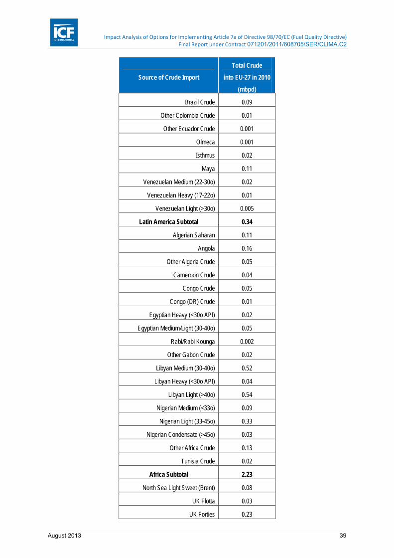
Impact Analysis of Options for Implementing Article 7a of Directive 98/70/EC (Fuel Quality Directive) Final Report under Contract 071201/2011/608705/SER/CLIMA.C2
August 2013 39
Source of Crude Import
Total Crude
into EU-27 in 2010
(mbpd)
Brazil Crude 0.09
Other Colombia Crude 0.01
Other Ecuador Crude 0.001
Olmeca 0.001
Isthmus 0.02
Maya 0.11
Venezuelan Medium (22-30o) 0.02
Venezuelan Heavy (17-22o) 0.01
Venezuelan Light (>30o) 0.005
Latin America Subtotal 0.34
Algerian Saharan 0.11
Angola 0.16
Other Algeria Crude 0.05
Cameroon Crude 0.04
Congo Crude 0.05
Congo (DR) Crude 0.01
Egyptian Heavy (<30o API) 0.02
Egyptian Medium/Light (30-40o) 0.05
Rabi/Rabi Kounga 0.002
Other Gabon Crude 0.02
Libyan Medium (30-40o) 0.52
Libyan Heavy (<30o API) 0.04
Libyan Light (>40o) 0.54
Nigerian Medium (<33o) 0.09
Nigerian Light (33-45o) 0.33
Nigerian Condensate (>45o) 0.03
Other Africa Crude 0.13
Tunisia Crude 0.02
Africa Subtotal 2.23
North Sea Light Sweet (Brent) 0.08
UK Flotta 0.03
UK Forties 0.23

Impact Analysis of Options for Implementing Article 7a of Directive 98/70/EC (Fuel Quality Directive) Final Report under Contract 071201/2011/608705/SER/CLIMA.C2
August 2013 40
Source of Crude Import
Total Crude
into EU-27 in 2010
(mbpd)
Other UK Crude 0.25
Norway 1.35
Denmark 0.15
Europe (local production) Subtotal 2.09
Russia Urals 1.75
Azerbaijan AIOC 0.40
Kazakhstan Crude 0.62
Other FSU Crude 0.29
Other Russian Fed. Crude 1.32
Ukraine Crude 0.002
FSU Subtotal 4.37
Iranian Hvy Sour (Azadegan) 0.30
Iraq Basrah 0.06
Iraq Kirkuk 0.23
Saudi Arabian Light 0.60
Saudi Arabian Heavy 0.0001
Murban 0.002
Upper Zakum 0.01
Other Iran Crude 0.11
Iranian Light 0.17
Other Iraq Crude 0.03
Kuwait Blend 0.07
Oman 0.003
Other Middle East Crude 0.0002
Arab Medium 0.0001
Berri (Extra Light) 0.02
Souedie 0.11
Syria Light 0.04
Masila Blend 0.005

Impact Analysis of Options for Implementing Article 7a of Directive 98/70/EC (Fuel Quality Directive) Final Report under Contract 071201/2011/608705/SER/CLIMA.C2
August 2013 41
Source of Crude Import
Total Crude
into EU-27 in 2010
(mbpd)
Middle East Subtotal 1.76
China Subtotal 0.00
Other Asia/Pac Subtotal 0.00
Total
(mbpd) 10.79
Source for 2010: EUROSTAT and OPEC.
Table 2.24 Summary of Notional Crude Trade in 2020
Source of Crude Import
Total Crude
into EU-27 in 2020
(mbpd)
USA & Canada Subtotal 0.00
Venez XHVY (Boscan) 0.065
Venezuelan JOBO 0.227
Venezuelan Syncrude 0.10
Venezuelan Heavy (17-22o) 0.127
Latin America Subtotal 0.518
Algerian Condensate 0.064
Algerian Saharan 0.944
Libyan 0.947
Egypt Suez Blend 0.062
Nigerian Bonny/Light 0.282
Nigerian Okono Etc Light 0.039
Nigerian Brass River/Escravos/Qua Iboe 0.327
Gabon Gamba 0.156
Angola 0.732
Angola Hitan (Kuito) 0.167
Benin 0.054
Zaire 0.033
Africa Subtotal 3.808

Impact Analysis of Options for Implementing Article 7a of Directive 98/70/EC (Fuel Quality Directive) Final Report under Contract 071201/2011/608705/SER/CLIMA.C2
August 2013 42
Source of Crude Import
Total Crude
into EU-27 in 2020
(mbpd)
North Sea Light Sweet (Brent) 0.423
North Sea Light Sour 0.175
North Sea Hitan Hvy Sweet 0.317
North Sea Condensate 0.122
Norway 0.346
Netherlands 0.027
Denmark 0.130
W. Germany 0.008
France 0.012
Austria 0.033
Spain 0.093
Italy 0.140
Greece 0.001
Turkey 0.015
Eastern Europe 0.124
Estonia Oil Shale 0.007
Europe (local production) Subtotal 1.974
Russia Urals 1.386
Azerbaijan AIOC 0.227
Turkmenistan Chelekan 0.002
FSU Subtotal 1.616
Iranian Hvy Sour (Azadegan) 0.007
Iraq Basrah 0.870
Iraq Kirkuk 0.348
Saudi Arabian Light 0.020
Saudi Arabian Heavy 0.001
Middle East Subtotal 1.247
China Subtotal 0.00

Impact Analysis of Options for Implementing Article 7a of Directive 98/70/EC (Fuel Quality Directive) Final Report under Contract 071201/2011/608705/SER/CLIMA.C2
August 2013 43
Source of Crude Import
Total Crude
into EU-27 in 2020
(mbpd)
Other Asia/Pac Subtotal 0.00
Total
(mbpd) 9.162
% Sweet Crude 51%
Source for 2020: WORLD Model.
2.6.6 Refinery Capacities and Utilisation
The WORLD base refinery capacity data accounted for announced refinery closures in Europe and elsewhere worldwide as shown in Table 2.25. The WORLD model for refinery data is for all of Europe not just the EU27. Refineries and the markets they serve cross EU27 boundaries. The low projected utilizations of 62% for 2020 imply substantial further closures are needed in Europe (4.4 mb/d to obtain 85%) which will be taken into account in the Task 3 competitiveness impact modelling by Vivid Economics. In general, refineries under 85% utilization have difficulty maintaining economically viable operations. It is likely therefore that there will be further reductions in EU refining capacity between now and 2020 regardless of the impact of the FQD (e.g. (Purvin & Gertz Inc., 2008) and (J.P Morgan, 2011). Many of these refineries are being converted into import terminals, which may alter the future competitiveness of imported refined product in the EU market.
Table 2.25 Announced European Refinery Closures
Country Company City WORLD Capacity (bbl/day)
Year Closed
Belgium PetroPlus Antwerp 107,500 2012
France PetroPlus Reichstett 78,000 2011
France PetroPlus Prtit Couronne 141,000 2012
France Total Dunkirk 140,700 2010
France Total Gonfreville 94,000 2011
Germany Bayernoil Ingolstadt 56,300 2009
Germany Shell Harburg 93,000 2012
Germany Philips66 Wilhelmshaven 260,000 2010
Italy Tamoil Cremona 94,000 2011
Italy ERG/Total Rome 89,109 2012
Romania Arpechim SA Pitesti 70,288 2010
Switzerland PetroPlus Cressier 60,000 2012
UK Petroplus Coryton 172,000 2012
UK Petroplus Teesside 100,000 2009
UK ExxonMobil Fawley 80,000 2012
Total European Capacity Reduction 1,635,897
Source: WORLD Model.

Impact Analysis of Options for Implementing Article 7a of Directive 98/70/EC (Fuel Quality Directive) Final Report under Contract 071201/2011/608705/SER/CLIMA.C2
August 2013 44
Table 2.26 Summary of Refinery Projects Accounted for in the WORLD Model (‘Europe’ region)
Company City Country Project Type
THOUSAND BARRELS PER DAY
2012 2013 2014 2015 2016 2017 2018 2019
Shell Pernis Netherlands Hydrotreater-Diesel 40 - - - - - - -
Total Gonfreville L'Orcher France Hydrocracker-Vacuum Gasoil - 40 - - - - - -
Agip/ENI Sannazzaro, Pavia Italy Hydrocracker-Resid - 23 - - - - - -
Galp Sines Portugal Hydrocracker-Vacuum Gasoil 43 - - - - - - -
Hellenic Petroleum Elefsis Greece Coker-Fluid/Flexi 20 - - - - - - -
Hellenic Petroleum Elefsis Greece Hydrocracker-Vacuum Gasoil 40 - - - - - - -
Hellenic Petroleum Elefsis Greece Hydrogen-Steam Methane (MMSCFD) 68 - - - - - - -
Hellenic Petroleum Elefsis Greece Vacuum 40 - - - - - - -
Hellenic Petroleum Thessaloniki Greece Crude 25 - - - - - - -
Hellenic Petroleum Thessaloniki Greece Reformer-CCR 15 - - - - - - -
Saras Sarroch Italy Hydrocracker-Other - 20 - - - - - -
STRAS (Socar & Turkas) Aliaga Turkey Coker-Delayed - - - - - 40 - -
STRAS (Socar & Turkas) Aliaga Turkey Crude - - - - - 214 - -
STRAS (Socar & Turkas) Aliaga Turkey Hydrocracker-Vacuum Gasoil - - - - - 66 - -
STRAS (Socar & Turkas) Aliaga Turkey Hydrogen-Steam Methane (MMSCFD) - - - - - 150 - -
STRAS (Socar & Turkas) Aliaga Turkey Hydrotreater-Diesel - - - - - 68 - -
STRAS (Socar & Turkas) Aliaga Turkey Hydrotreater-Kerosene - - - - - 26 - -
STRAS (Socar & Turkas) Aliaga Turkey Hydrotreater-Naphtha - - - - - 20 - -
STRAS (Socar & Turkas) Aliaga Turkey Reformer-CCR - - - - - 28 - -
STRAS (Socar & Turkas) Aliaga Turkey Sulphur (LT/D) - - - - - 300 - -
STRAS (Socar & Turkas) Aliaga Turkey Vacuum - - - - - 80 - -

Impact Analysis of Options for Implementing Article 7a of Directive 98/70/EC (Fuel Quality Directive) Final Report under Contract 071201/2011/608705/SER/CLIMA.C2
August 2013 45
Company City Country Project Type
THOUSAND BARRELS PER DAY
2012 2013 2014 2015 2016 2017 2018 2019
Tupras Izmit Turkey Coker-Delayed - - - 52 - - - -
Tupras Izmit Turkey Hydrocracker-Vacuum Gasoil - - - 50 - - - -
Tupras Izmit Turkey Hydrogen-Steam Methane (MMSCFD) - - - 100 - - - -
Tupras Izmit Turkey Hydrotreater-Diesel - - - 28 - - - -
Tupras Izmit Turkey Hydrotreater-Petrol - - - 7 - - - -
Tupras Izmit Turkey Sulphur (LT/D) - - - 360 - - - -
Tupras Izmit Turkey Vacuum - - - 47 - - - -
INA Rijeka Croatia Hydrogen-Steam Methane (MMSCFD) 75 - - - - - - -
INA Rijeka Croatia Hydrotreater-Diesel 18 - - - - - - -
INA Rijeka Croatia Sulphur (LT/D) 190 - - - - - - -
Lukoil Neftochim Bourgas Bulgaria Hydrocracker-Resid - - - 43 - - - -
Lukoil Neftochim Bourgas Bulgaria Hydrocracker-Vacuum Gasoil - - - 35 - - - -
Lukoil Neftochim Bourgas Bulgaria Hydrogen-Steam Methane (MMSCFD) - - - 142 - - - -
NIS Pancevo Serbia Hydrocracker-Other - 65 - - - - - -
NIS Pancevo Serbia Isomerization-C5/C6 - 10 - - - - - -
NIS Pancevo Serbia Reformer-CCR - 17 - - - - - -
OMV Petrom (Petrobrazi) Ploiesti Romania Coker-Delayed - - 7 - - - - -
OMV Petrom (Petrobrazi) Ploiesti Romania Hydrocracker-Vacuum Gasoil - - 34 - - - - -
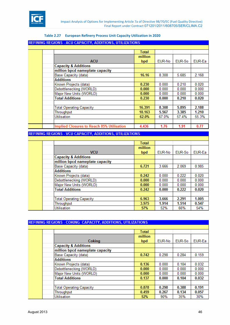
Impact Analysis of Options for Implementing Article 7a of Directive 98/70/EC (Fuel Quality Directive) Final Report under Contract 071201/2011/608705/SER/CLIMA.C2
August 2013 46
Table 2.27 European Refinery Process Unit Capacity Utilization in 2020

Impact Analysis of Options for Implementing Article 7a of Directive 98/70/EC (Fuel Quality Directive) Final Report under Contract 071201/2011/608705/SER/CLIMA.C2
August 2013 47
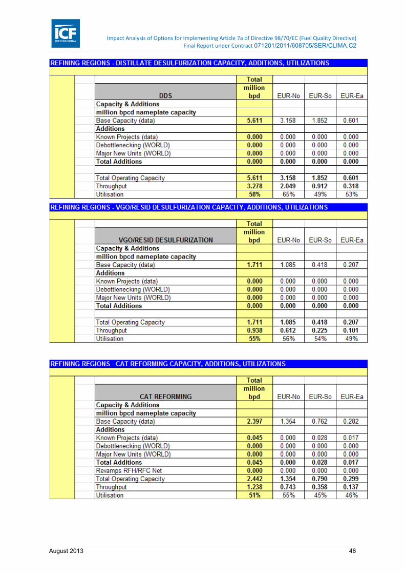
Impact Analysis of Options for Implementing Article 7a of Directive 98/70/EC (Fuel Quality Directive) Final Report under Contract 071201/2011/608705/SER/CLIMA.C2
August 2013 48

Impact Analysis of Options for Implementing Article 7a of Directive 98/70/EC (Fuel Quality Directive) Final Report under Contract 071201/2011/608705/SER/CLIMA.C2
August 2013 49
Table 2.28 Global Refinery Process Unit Capacity Utilization in 2020
* World Additions are capacity additions calculated by the World model
REFINING REGIONS - ACU CAPACITY, ADDITIONS, UTILIZATIONS
Total
ACUmillion
bpd USA&Canada Latin America Africa Europe FSU Middle East China Other Asia/PacCapacity & Additionsmillion bpcd nameplate capacityBase Capacity + Firm Projects 99.97 20.218 8.557 4.042 16.391 9.089 9.812 12.746 19.118
WORLD Additions (Debot + Major New Units) 0.442 0.118 0.000 0.035 0.000 0.000 0.126 0.163 0.000
Total Operating Capacity 100.416 20.336 8.557 4.077 16.391 9.089 9.938 12.909 19.118Throughput 78.571 17.774 5.940 3.059 10.213 6.451 8.322 12.214 14.600Utilisation 78% 87% 69% 75% 62% 71% 84% 95% 76%
Implied Closures to Reach 85% Utilisation 10.013 0.00 1.57 0.48 4.38 1.50 0.15 0.00 1.94
REFINING REGIONS - VCU CAPACITY, ADDITIONS, UTILIZATIONS
Total
VCUmillion
bpd USA&Canada Latin America Africa Europe FSU Middle East China Other Asia/PacCapacity & Additionsmillion bpcd nameplate capacityBase Capacity + Firm Projects 38.84 9.213 3.711 1.122 6.963 3.369 3.207 4.933 6.323
WORLD Additions (Debot + Major New Units) 0.060 0.014 0.000 0.005 0.000 0.000 0.041 0.000 0.000
Total Operating Capacity 38.901 9.227 3.711 1.127 6.963 3.369 3.248 4.933 6.323Throughput 24.008 6.455 1.695 0.794 3.966 1.719 2.525 3.837 3.017Utilisation 62% 70% 46% 70% 57% 51% 78% 78% 48%

Impact Analysis of Options for Implementing Article 7a of Directive 98/70/EC (Fuel Quality Directive) Final Report under Contract 071201/2011/608705/SER/CLIMA.C2
August 2013 50
REFINING REGIONS - COKING CAPACITY, ADDITIONS, UTILIZATIONS
Total
Cokingmillion
bpd USA&Canada Latin America Africa Europe FSU Middle East China Other Asia/PacCapacity & Additionsmillion bpcd nameplate capacityBase Capacity + Firm Projects 8.35 3.119 1.058 0.133 0.878 0.417 0.253 1.561 0.931
WORLD Additions (Debot + Major New Units) 0.032 0.026 0.001 0.000 0.001 0.001 0.000 0.000 0.003
Total Operating Capacity 8.381 3.145 1.059 0.134 0.878 0.418 0.253 1.561 0.934Throughput 4.815 2.527 0.489 0.024 0.441 0.119 0.061 0.848 0.307Utilisation 57% 80% 46% 18% 50% 28% 24% 54% 33%
REFINING REGIONS - FCC CAPACITY, ADDITIONS, UTILIZATIONS
Total
FCCmillion
bpd USA&Canada Latin America Africa Europe FSU Middle East China Other Asia/PacCapacity & Additionsmillion bpcd nameplate capacityBase Capacity + Firm Projects 18.19 6.265 1.753 0.312 2.277 0.855 1.014 2.703 3.010
WORLD Additions (Debot + Major New Units) 0.031 0.000 0.000 0.002 0.000 0.029 0.000 0.000 0.000
Total Operating Capacity 18.219 6.265 1.753 0.313 2.277 0.884 1.014 2.703 3.010Throughput 11.589 4.090 1.286 0.214 1.204 0.542 0.635 2.077 1.541Utilisation 64% 65% 73% 68% 53% 61% 63% 77% 51%
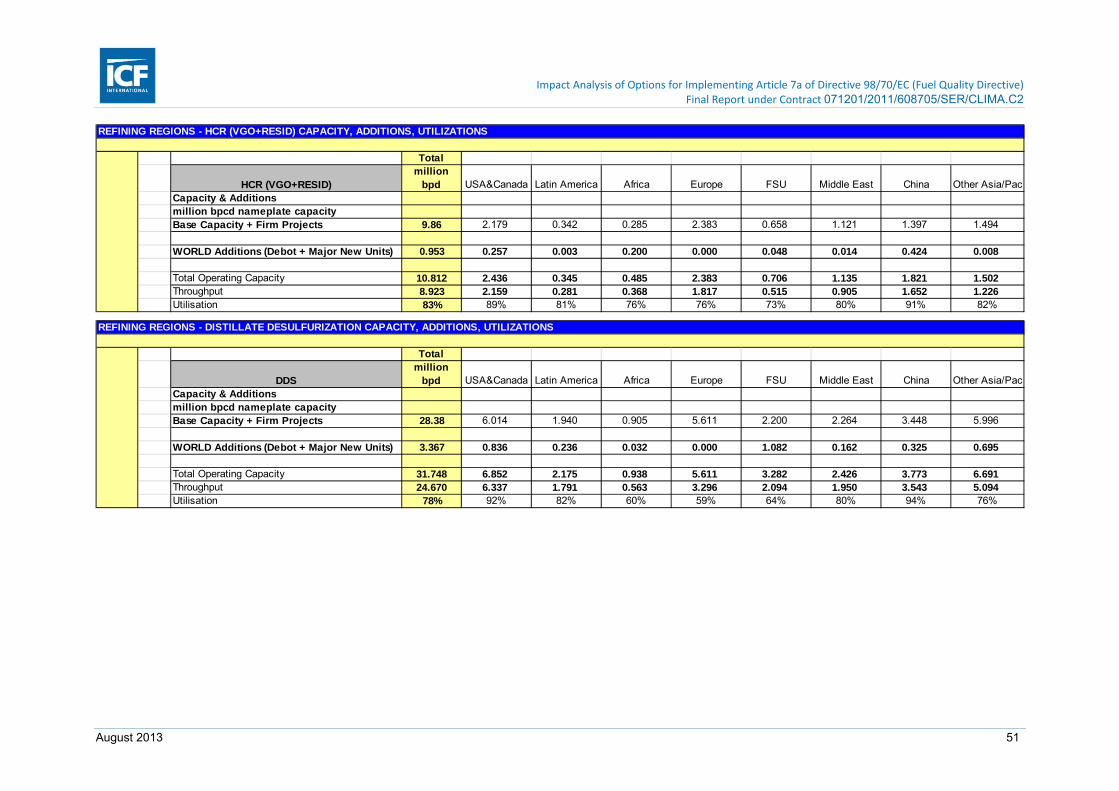
Impact Analysis of Options for Implementing Article 7a of Directive 98/70/EC (Fuel Quality Directive) Final Report under Contract 071201/2011/608705/SER/CLIMA.C2
August 2013 51
REFINING REGIONS - HCR (VGO+RESID) CAPACITY, ADDITIONS, UTILIZATIONS
Total
HCR (VGO+RESID)million
bpd USA&Canada Latin America Africa Europe FSU Middle East China Other Asia/PacCapacity & Additionsmillion bpcd nameplate capacityBase Capacity + Firm Projects 9.86 2.179 0.342 0.285 2.383 0.658 1.121 1.397 1.494
WORLD Additions (Debot + Major New Units) 0.953 0.257 0.003 0.200 0.000 0.048 0.014 0.424 0.008
Total Operating Capacity 10.812 2.436 0.345 0.485 2.383 0.706 1.135 1.821 1.502Throughput 8.923 2.159 0.281 0.368 1.817 0.515 0.905 1.652 1.226Utilisation 83% 89% 81% 76% 76% 73% 80% 91% 82%
REFINING REGIONS - DISTILLATE DESULFURIZATION CAPACITY, ADDITIONS, UTILIZATIONS
Total
DDSmillion
bpd USA&Canada Latin America Africa Europe FSU Middle East China Other Asia/PacCapacity & Additionsmillion bpcd nameplate capacityBase Capacity + Firm Projects 28.38 6.014 1.940 0.905 5.611 2.200 2.264 3.448 5.996
WORLD Additions (Debot + Major New Units) 3.367 0.836 0.236 0.032 0.000 1.082 0.162 0.325 0.695
Total Operating Capacity 31.748 6.852 2.175 0.938 5.611 3.282 2.426 3.773 6.691Throughput 24.670 6.337 1.791 0.563 3.296 2.094 1.950 3.543 5.094Utilisation 78% 92% 82% 60% 59% 64% 80% 94% 76%
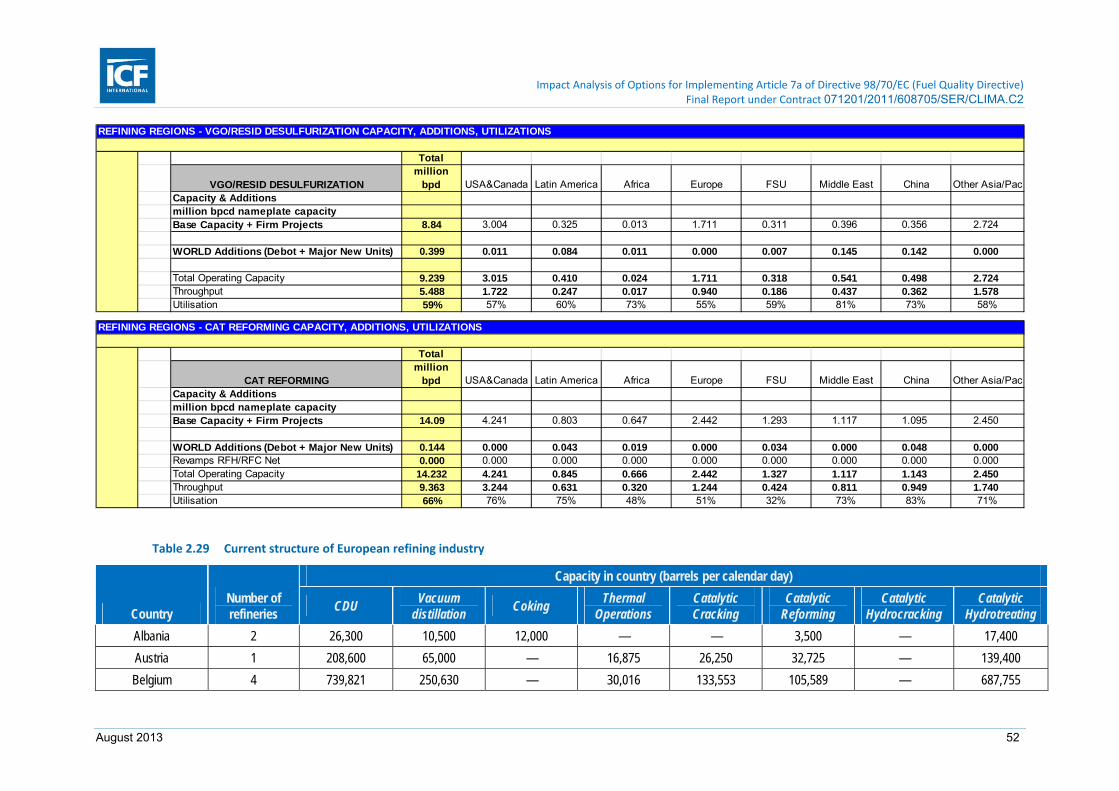
Impact Analysis of Options for Implementing Article 7a of Directive 98/70/EC (Fuel Quality Directive) Final Report under Contract 071201/2011/608705/SER/CLIMA.C2
August 2013 52
Table 2.29 Current structure of European refining industry
Country Number of refineries
Capacity in country (barrels per calendar day)
CDU Vacuum
distillation Coking
Thermal Operations
Catalytic Cracking
Catalytic Reforming
Catalytic Hydrocracking
Catalytic Hydrotreating
Albania 2 26,300 10,500 12,000 — — 3,500 — 17,400
Austria 1 208,600 65,000 — 16,875 26,250 32,725 — 139,400
Belgium 4 739,821 250,630 — 30,016 133,553 105,589 — 687,755
REFINING REGIONS - VGO/RESID DESULFURIZATION CAPACITY, ADDITIONS, UTILIZATIONS
Total
VGO/RESID DESULFURIZATIONmillion
bpd USA&Canada Latin America Africa Europe FSU Middle East China Other Asia/PacCapacity & Additionsmillion bpcd nameplate capacityBase Capacity + Firm Projects 8.84 3.004 0.325 0.013 1.711 0.311 0.396 0.356 2.724
WORLD Additions (Debot + Major New Units) 0.399 0.011 0.084 0.011 0.000 0.007 0.145 0.142 0.000
Total Operating Capacity 9.239 3.015 0.410 0.024 1.711 0.318 0.541 0.498 2.724Throughput 5.488 1.722 0.247 0.017 0.940 0.186 0.437 0.362 1.578Utilisation 59% 57% 60% 73% 55% 59% 81% 73% 58%
REFINING REGIONS - CAT REFORMING CAPACITY, ADDITIONS, UTILIZATIONS
Total
CAT REFORMINGmillion
bpd USA&Canada Latin America Africa Europe FSU Middle East China Other Asia/PacCapacity & Additionsmillion bpcd nameplate capacityBase Capacity + Firm Projects 14.09 4.241 0.803 0.647 2.442 1.293 1.117 1.095 2.450
WORLD Additions (Debot + Major New Units) 0.144 0.000 0.043 0.019 0.000 0.034 0.000 0.048 0.000Revamps RFH/RFC Net 0.000 0.000 0.000 0.000 0.000 0.000 0.000 0.000 0.000Total Operating Capacity 14.232 4.241 0.845 0.666 2.442 1.327 1.117 1.143 2.450Throughput 9.363 3.244 0.631 0.320 1.244 0.424 0.811 0.949 1.740Utilisation 66% 76% 75% 48% 51% 32% 73% 83% 71%

Impact Analysis of Options for Implementing Article 7a of Directive 98/70/EC (Fuel Quality Directive) Final Report under Contract 071201/2011/608705/SER/CLIMA.C2
August 2013 53
Country Number of refineries
Capacity in country (barrels per calendar day)
CDU Vacuum
distillation Coking
Thermal Operations
Catalytic Cracking
Catalytic Reforming
Catalytic Hydrocracking
Catalytic Hydrotreating
Bulgaria 1 115,240 49,900 — 20,600 23,300 4,060 — 64,200
Croatia 3 250,317 87,040 5,000 23,526 51,002 49,368 12,264 68,256
Czech Republic 3 183,000 78,870 — 17,000 — 27,470 34,430 103,780
Denmark 2 174,400 22,000 — 64,550 — 21,990 — 42,760
Finland 2 260,575 146,085 — 34,420 56,690 50,060 90,110 298,325
France 12 1,718,803 715,200 — 146,872 347,052 256,669 71,845 1,233,048
Germany 15 2,417,162 1,096,231 105,809 247,445 349,171 404,822 203,067 2,011,782
Greece 4 423,000 152,000 — 49,000 75,550 49,200 43,900 361,635
Hungary 1 161,000 77,500 16,900 14,000 24,000 29,600 — 120,700
Ireland 1 71,000 — — — — 11,000 — 44,600
Italy 17 2,337,229 814,237 45,000 448,204 321,500 287,069 303,210 1,250,753
Lithuania 1 190,000 89,300 — 28,800 43,200 45,900 — 153,900
Macedonia 1 50,000 — — — — 10,860 — 22,050
Netherlands 6 1,196,571 711,095 41,500 91,404 101,983 148,616 198,071 1,016,234
Norway 2 319,000 — 24,780 32,000 49,000 34,900 — 126,000
Poland 4 492,950 265,123 — — 32,985 67,514 145,908 259,507
Portugal 2 304,172 87,785 — 36,540 40,500 50,182 9,180 201,537
Romania 10 537,277 273,225 68,240 37,577 109,478 61,763 1,534 237,625
Serbia & Montenegro
2 214,826 50,583 — 20,340 18,950 18,822 — 50,910
Slovakia 1 115,000 55,000 — — 18,000 21,000 42,000 87,800
Slovenia 1 13,500 — — — — — — —
Spain 9 1,271,500 414,245 61,100 149,200 191,300 196,750 131,500 825,380
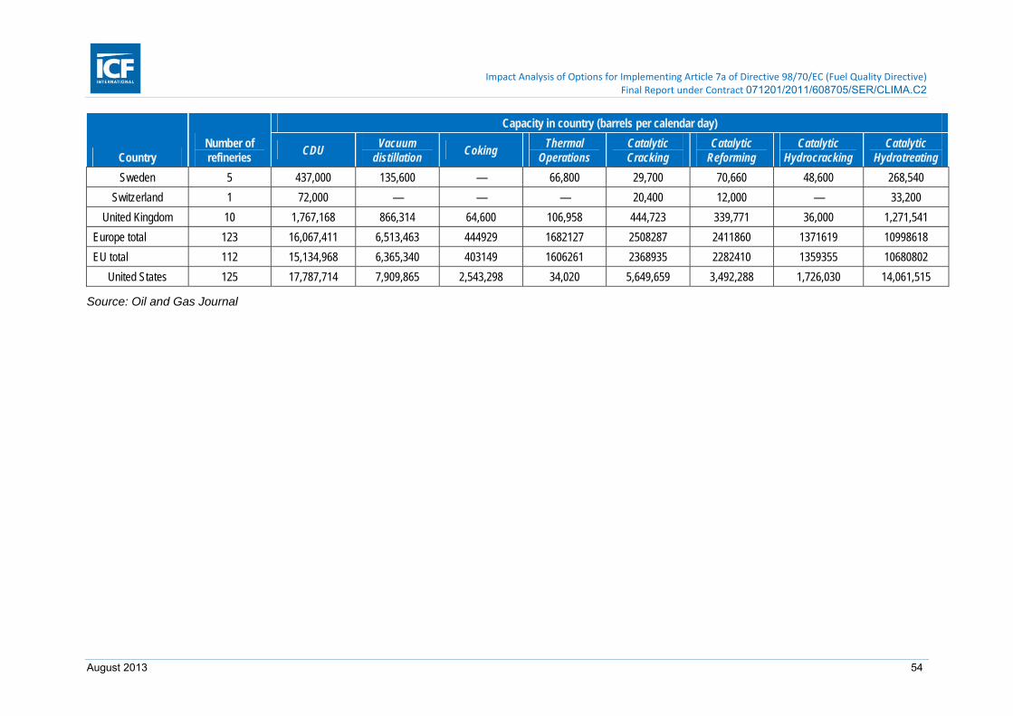
Impact Analysis of Options for Implementing Article 7a of Directive 98/70/EC (Fuel Quality Directive) Final Report under Contract 071201/2011/608705/SER/CLIMA.C2
August 2013 54
Country Number of refineries
Capacity in country (barrels per calendar day)
CDU Vacuum
distillation Coking
Thermal Operations
Catalytic Cracking
Catalytic Reforming
Catalytic Hydrocracking
Catalytic Hydrotreating
Sweden 5 437,000 135,600 — 66,800 29,700 70,660 48,600 268,540
Switzerland 1 72,000 — — — 20,400 12,000 — 33,200
United Kingdom 10 1,767,168 866,314 64,600 106,958 444,723 339,771 36,000 1,271,541
Europe total 123 16,067,411 6,513,463 444929 1682127 2508287 2411860 1371619 10998618
EU total 112 15,134,968 6,365,340 403149 1606261 2368935 2282410 1359355 10680802
United States 125 17,787,714 7,909,865 2,543,298 34,020 5,649,659 3,492,288 1,726,030 14,061,515
Source: Oil and Gas Journal
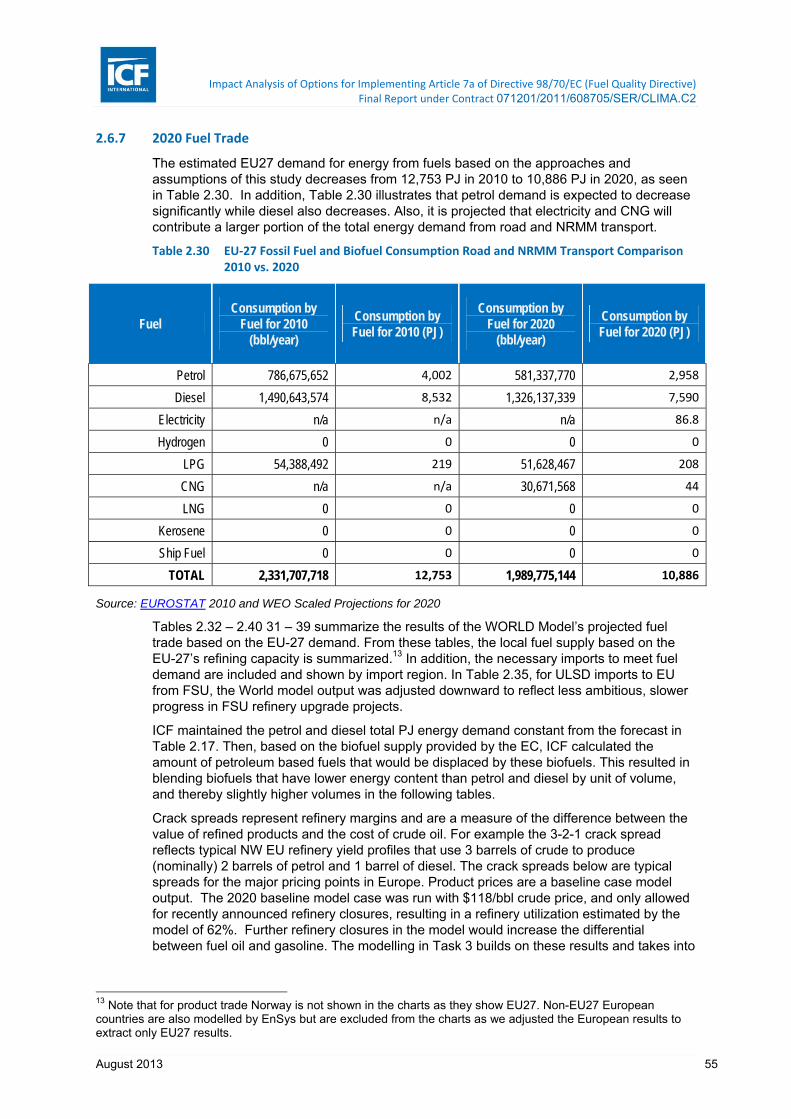
Impact Analysis of Options for Implementing Article 7a of Directive 98/70/EC (Fuel Quality Directive) Final Report under Contract 071201/2011/608705/SER/CLIMA.C2
August 2013 55
2.6.7 2020 Fuel Trade
The estimated EU27 demand for energy from fuels based on the approaches and assumptions of this study decreases from 12,753 PJ in 2010 to 10,886 PJ in 2020, as seen in Table 2.30. In addition, Table 2.30 illustrates that petrol demand is expected to decrease significantly while diesel also decreases. Also, it is projected that electricity and CNG will contribute a larger portion of the total energy demand from road and NRMM transport.
Table 2.30 EU‐27 Fossil Fuel and Biofuel Consumption Road and NRMM Transport Comparison 2010 vs. 2020
Fuel Consumption by
Fuel for 2010 (bbl/year)
Consumption by Fuel for 2010 (PJ)
Consumption by Fuel for 2020
(bbl/year)
Consumption by Fuel for 2020 (PJ)
Petrol 786,675,652 4,002 581,337,770 2,958
Diesel 1,490,643,574 8,532 1,326,137,339 7,590
Electricity n/a n/a n/a 86.8
Hydrogen 0 0 0 0
LPG 54,388,492 219 51,628,467 208
CNG n/a n/a 30,671,568 44
LNG 0 0 0 0
Kerosene 0 0 0 0
Ship Fuel 0 0 0 0
TOTAL 2,331,707,718 12,753 1,989,775,144 10,886
Source: EUROSTAT 2010 and WEO Scaled Projections for 2020
Tables 2.32 – 2.40 31 – 39 summarize the results of the WORLD Model’s projected fuel trade based on the EU-27 demand. From these tables, the local fuel supply based on the EU-27’s refining capacity is summarized.13 In addition, the necessary imports to meet fuel demand are included and shown by import region. In Table 2.35, for ULSD imports to EU from FSU, the World model output was adjusted downward to reflect less ambitious, slower progress in FSU refinery upgrade projects.
ICF maintained the petrol and diesel total PJ energy demand constant from the forecast in Table 2.17. Then, based on the biofuel supply provided by the EC, ICF calculated the amount of petroleum based fuels that would be displaced by these biofuels. This resulted in blending biofuels that have lower energy content than petrol and diesel by unit of volume, and thereby slightly higher volumes in the following tables.
Crack spreads represent refinery margins and are a measure of the difference between the value of refined products and the cost of crude oil. For example the 3-2-1 crack spread reflects typical NW EU refinery yield profiles that use 3 barrels of crude to produce (nominally) 2 barrels of petrol and 1 barrel of diesel. The crack spreads below are typical spreads for the major pricing points in Europe. Product prices are a baseline case model output. The 2020 baseline model case was run with $118/bbl crude price, and only allowed for recently announced refinery closures, resulting in a refinery utilization estimated by the model of 62%. Further refinery closures in the model would increase the differential between fuel oil and gasoline. The modelling in Task 3 builds on these results and takes into
13 Note that for product trade Norway is not shown in the charts as they show EU27. Non-EU27 European countries are also modelled by EnSys but are excluded from the charts as we adjusted the European results to extract only EU27 results.
Impact Analysis of Options for Implementing Article 7a of Directive 98/70/EC (Fuel Quality Directive) Final Report under Contract 071201/2011/608705/SER/CLIMA.C2
August 2013 56
account the amount of additional closures necessary to achieve economically viable utilisation levels.
The tables in the following section contain some aggregated fuels including:
■ Total Distillate is diesel on/off road 10 ppm, gas oil, heating oil, and marine distillate
■ Total Residual is aggregated residual fuels including marine IFO.
■ Total Petrochemical Naphtha is feedstock destined for the petrochemical industry (e.g. ethylene manufacture or aromatics production)
■ LPG includes transport, and residential and commercial
2.6.8 Factors Contributing to European Diesel and Petrol Market
2.6.8.1 Overview
While several factors contribute to the current situation of the European diesel and petrol market, the structural decline in regional product demand is most relevant. Global oil product balances will change by 2020 from the current situation in particular the transformation of the North American market. North America, a net importer of some 900 kb/d of refined products in 2000, swung to net exporter status in 2009, and by 2011 had a surplus of some 600 kb/d.14 US product exports led the shift, averaging 2.6 mb/d in 2011, or more than 1 mb/d on a net basis, partly offset by rising imports from Mexico. The changes in the European oil markets are equally significant. European net imports of oil products were more than halved during the last decade, to just over 500 kb/d in total in 2011. The region’s middle distillate imports averaged 830 kb/d, offset by petrol exports of 820 kb/d, while other products amounted to 500 kb/d of net imports (IEA Midterm 2012). A structural shift in demand, from petrol to diesel, is continuing to cause Europe’s refiners problems as they have to find outlets for surplus petrol production, often at discounted prices. North America remains the largest purchaser of petrol, though exports to Africa and the Middle East from Europe are on the rise. The FSU is the main supplier of refined products to Europe with combined exports of 1.3 mb/d in 2011. In 2020, EU27’s petrol surplus will be approximately 0.93 mb/d based on ICF’s forecast, while diesel and gas oil imports could surge to more than 1.01 mb/d as a result of capacity rationalization and lower throughputs. In the non-OECD, the FSU will remain the largest product exporter globally, with increasing export potential of both light and middle distillates through 2020 while refinery upgrades cut into fuel oil supplies.
2.6.8.2 Distillates / diesel
Regionally, Europe has the largest deficit in middle distillate supplies. The largest share of the imports have come from the FSU, but increasing volumes are also being sourced from North America. In 2020, Europe’s distillate deficit will most likely rise, with additional volumes possibly sourced from the FSU, USA/Canada, Middle East, India and Africa, with higher export potential when FSU refinery upgrades and new construction projects are completed. Middle East product exports are projected as going primarily to Asia where the demand growth is but changes in circumstances, such as a reduction in US or Russian ability to export product distillate to Europe could lead to changes in these flows. North America should retain some export potential, despite internal distillates demand growth. (U.S. refineries have been steadily shifting their yields away from petrol toward distillate, including via costly hydro-cracker projects.)
The major source of imports of 10ppm diesel into the EU is FSU. Key factors driving imports from FSU into the EU in the model include those listed below. The premises chosen for any and all of these (and other factors) can and will impact WORLD model results for EU imports as well as other activities worldwide. The following are illustrations of factors which we believe are potentially significant. They do not represent an exhaustive list.
14 International Energy Agency Midterm 2012

Impact Analysis of Options for Implementing Article 7a of Directive 98/70/EC (Fuel Quality Directive) Final Report under Contract 071201/2011/608705/SER/CLIMA.C2
August 2013 57
■ Feedstocks / products
– Supply / demand projections:
○ In the EU the model has lower demand for diesel, but also lower refinery production due to the sector’s reduced competitiveness compared to other regions as a result of the projected carbon price of €16.5/ tCO2e which thus leads to more diesel imports
○ Surplus capacity available for export production: there is assumed to be investment in additional capacity in FSU in the base case run – a key sensitivity is the extent to which these additional investments in fact go ahead
○ The model demand premises, based on the IEA WEO, include significant demand growth in Asia, with the Middle East and Indian diesel exports being directed to that market. If there was lower growth in Asia, the exports from the Middle East and India would in part be targeted elsewhere including the EU and would therefore compete more strongly with exports from FSU and USA/Canada into the EU. This trade outlook will also be affected by assumptions on how much refinery capacity will grow in India, China, and the Middle East.
○ There has been recent growth in distillate exports from US to Latin America – however new capacity is coming on line in Latin America which may mean that US exports would increasingly target other regions including the EU. The ability of the US to export diesel will also be affected by any potential regulations adding costs to US refineries (e.g. future stationary source emissions, product quality or climate policies) which would tend to reduce their competitiveness.
– Product quality standards in different world regions: the 2020 WORLD model run included the premise that Russia moves steadily but not rapidly towards ULSD standards. As a result, a relatively large quantity of ULSD from FSU is available for export in comparison to a scenario (e.g. according to some 3rd party projections) where Russia moves more quickly to ULSD standards, in which case less ULS fuel would be available for export.
■ Refinery production/yields
– Limits of diesel to petrol production ratio: production of diesel is linked to production of petrol – it is not possible to produce any mix of diesel to petrol. As such, the EU’s ability to produce diesel is constrained by its ability to export petrol; similarly for potential importers depending in part on their refinery configurations
– Investment in new capacity: for a ‘long run’ case such as the case modelled for this study (2020 projection) the model allows the opportunity for investment in new capacity over and above base capacity plus firm projects. Further additions are generally allowed in all regions but tend to occur in those where demand is growing. The modelling approach endogenously considers the economics of building new regional capacity vs. not building new capacity and increasing products imports instead. For example, China tends to have low costs of construction (plus strong government support for domestic capacity growth) and hence tends to import crude more so than product, whereas in Africa refining capacity is largely inefficient, costs for new projects are high and ability to finance and implement low, hence the tendency is to import product not crude. Given the integrated nature of the model, these factors are important in determining product import/export flows.
■ Transport
– Transport capacity and costs will have an important impact on movements of products. Marine movements link regions together but the attractiveness of those movements depends on their cost.
2.6.8.3 Petrol
The most significant change to global petrol product balances derives from the changing North American energy landscape. The US is moving from being the world’s largest importer

Impact Analysis of Options for Implementing Article 7a of Directive 98/70/EC (Fuel Quality Directive) Final Report under Contract 071201/2011/608705/SER/CLIMA.C2
August 2013 58
of petrol to a position of much greater self-sufficiency, balancing East Coast imports15 with growing Gulf Coast exports to neighbouring Mexico and several Latin American countries. North American net petrol imports fell to roughly 600 kb/d in 2011 from a 2006 peak of 1.08 mb/d, due to several factors (IEA Midterm 2012). US Gulf Coast and Midcontinent refiners enjoy a competitive advantage in the form of discounted crude feedstock (WTI) and refinery fuel (natural gas) and have been running at a relatively high utilization. The decline of North American petrol imports is a challenge for European refiners, which traditionally have provided around 70% of regional imports. Since the mid-90s, the dieselization of the European car fleet and shrinking demand have caused Europe to become increasingly oversupplied with petrol.
2.6.8.4 EU refining industry
The pressures on the European refining industry will continue. In 2020, EU27’s diesel and petrol product demand is set to continue to decline, from 6.2 mb/d in 2010 to 5.2 mb/d in 2020. Given this demand outlook, and in the absence of further project delays or cancellations, refinery closures in Europe of more than 4 mb/d by 2020 could be needed to achieve a healthy utilization rate of 85%16. In general, utilization rates are expected to fall more sharply in the OECD than in the non-OECD, as demand continues to shift towards developing nations.
It is possible that national oil companies in Russia, Brazil and the Middle East will act to keep their refineries full, choosing to export finished products produced from their own crude and capturing more of the value added from refining domestically. Although refining economics tend to favour processing closer to end use markets, an integrated supply chain and the power to price crude into domestic refineries will likely see a significant presence in the market from export-oriented national oil company refineries.
Table 2.31 Crack Spreads in “Northern Europe” WORLD Model Region
Crack Spreads ($/bbl) in Northern Europe Region
NW Europe 3-2-1 Brent $ 6.12
NW Europe 2-1-1 Brent $ 10.22
NW Europe 5-2-2-1 Brent $ 6.76
Brent, regular grade petrol 95 RON, ULSD 10ppm, and - for 5-2-2-1 – IFO 380 (intermediate fuel oil at 380 centistokes).
Table 2.32 Summary of Product Prices in 2020 WORLD Model Projection
Product EUR-No EUR-So EUR-Ea
$/bbl $/bbl $/bbl
LPG $ 106.86 $ 106.24 $ 108.26
PETCHEM NAPHTHA $ 108.54 $ 107.62 $ 109.73
15 The projection of sustained petrol imports into the US from EU by 2020 reflected recent refinery closures and capacity reduction in the region and was also based on the endogenous result/projection that East Coast refineries and throughputs would continue to be under pressure. However the logistics of US domestic crude oil supply into East Coast refineries is changing rapidly. It is not conclusive if recent domestic unconventional tight oil supplies into the northeast via rail will remain a long term trend. However these developments could, especially if also supported by regional tight oil growth (notably the Utica shale), act to sustain East Coast refining activity. 16 There are many refiners running at below 85% capacity utilization which generate added-value, have vertical integration (e.g. with petrochemicals) or other strategic, social or economic benefits for their operators, so the assumptions on how much capacity might be prone to closure are simplistic.

Impact Analysis of Options for Implementing Article 7a of Directive 98/70/EC (Fuel Quality Directive) Final Report under Contract 071201/2011/608705/SER/CLIMA.C2
August 2013 59
PETROL - PREMIUM $ 120.13 $ 116.32 $ 118.54
PETROL - REGULAR $ 117.65 $ 113.81 $ 115.78
JET A1 $ 139.65 $ 138.01 $ 136.84
ULSD $ 142.24 $ 140.75 $ 139.84
RESID .3-1.0% $ 114.14 $ 116.51 $ 117.90
IFO380 HS $ 112.68 $ 112.26 $ 116.26
Regular grade petrol 95 RON, premium, ULSD 10ppm, and IFO 380.

Impact Analysis of Options for Implementing Article 7a of Directive 98/70/EC (Fuel Quality Directive) Final Report under Contract 071201/2011/608705/SER/CLIMA.C2
August 2013 60
Table 2.33 2020 Petrol Trade (Fossil and Biofuel)
Region Total Exports
(mbpd)
Total Local + Exports (mbpd)
USA&Canada (mbpd)
Latin America (mbpd)
Africa (mbpd)
EU-27 (mbpd)
FSU (mbpd)
Middle East (mbpd)
China (mbpd)
Other Asia/Pac (mbpd)
USA & Canada 0.57 8.76 8.18 0.51 0.03 0.00 0.00 0.00 0.04 0.00
Latin America 0.26 2.24 0.26 1.98 0.00 0.00 0.00 0.00 0.00 0.00
Africa 0.09 0.84 0.09 0.00 0.75 0.00 0.00 0.00 0.00 0.00
EU-27 0.93 2.60 0.61 0.00 0.26 1.67 0.06 0.00 0.00 0.00
FSU 0.00 1.20 0.00 0.00 0.00 0.00 1.20 0.00 0.00 0.00
Middle East 0.20 1.78 0.00 0.00 0.01 0.00 0.00 1.58 0.00 0.19
China 0.07 2.65 0.00 0.00 0.00 0.00 0.00 0.00 2.58 0.07
Other Asia/Pac 0.09 3.38 0.07 0.00 0.02 0.00 0.00 0.00 0.00 3.28
Total Imports 2.21 1.02 0.51 0.33 0.00 0.06 0.00 0.04 0.26
TOTAL Imports + Local 23.43 9.20 2.49 1.08 1.67 1.26 1.58 2.62 3.54
Source: WORLD Model.

Impact Analysis of Options for Implementing Article 7a of Directive 98/70/EC (Fuel Quality Directive) Final Report under Contract 071201/2011/608705/SER/CLIMA.C2
August 2013 61
Table 2.34 2020 Jet/Kerosene Trade
Region Total Exports
(mbpd)
Total Local + Exports (mbpd)
USA&Canada (mbpd)
Latin America (mbpd)
Africa (mbpd)
EU-27 (mbpd)
FSU (mbpd)
Middle East (mbpd)
China (mbpd)
Other Asia/Pac (mbpd)
USA & Canada 0.38 2.32 1.94 0.09 0.09 0.00 0.00 0.00 0.00 0.20
Latin America 0.00 0.29 0.00 0.29 0.00 0.00 0.00 0.00 0.00 0.00
Africa 0.03 0.26 0.00 0.00 0.23 0.03 0.00 0.00 0.00 0.00
EU-27 0.03 1.01 0.00 0.00 0.03 0.98 0.00 0.00 0.00 0.00
FSU 0.17 0.51 0.00 0.00 0.00 0.04 0.35 0.00 0.00 0.13
Middle East 0.52 1.02 0.00 0.00 0.02 0.00 0.00 0.50 0.00 0.49
China 0.15 0.65 0.00 0.00 0.00 0.00 0.00 0.00 0.50 0.15
Other Asia/Pac 0.00 1.13 0.00 0.00 0.00 0.00 0.00 0.00 0.00 1.13
Total Imports 1.28 0.00 0.09 0.15 0.07 0.00 0.00 0.00 0.97
TOTAL Imports + Local 7.20 1.94 0.39 0.38 1.04 0.35 0.50 0.50 2.10
Source: WORLD Model.

Impact Analysis of Options for Implementing Article 7a of Directive 98/70/EC (Fuel Quality Directive) Final Report under Contract 071201/2011/608705/SER/CLIMA.C2
August 2013 62
Table 2.35 Total ULSD Trade (Fossil and Biofuel)
Region Total Exports
(mbpd)
Total Local + Exports (mbpd)
USA&Canada (mbpd)
Latin America (mbpd)
Africa (mbpd)
EU-27 (mbpd)
FSU (mbpd)
Middle East (mbpd)
China (mbpd)
Other Asia/Pac (mbpd)
USA & Canada 0.10 4.35 4.24 0.00 0.00 0.10 0.00 0.00 0.00 0.00
Latin America 0.00 0.47 0.00 0.47 0.00 0.00 0.00 0.00 0.00 0.00
Africa 0.00 0.27 0.00 0.00 0.27 0.00 0.00 0.00 0.00 0.00
EU-27 0.00 2.99 0.00 0.00 0.00 3.14 0.00 0.00 0.00 0.00
FSU 0.86 1.07 0.00 0.00 0.00 0.41 0.12 0.00 0.00 0.00
Middle East 0.03 0.71 0.00 0.00 0.00 0.00 0.00 0.68 0.00 0.03
China 0.00 1.12 0.00 0.00 0.00 0.00 0.00 0.00 1.12 0.00
Other Asia/Pac 0.00 2.10 0.00 0.00 0.00 0.00 0.00 0.00 0.00 2.10
Total Imports 0.99 0.00 0.00 0.00 0.51 0.00 0.00 0.00 0.03
TOTAL Imports + Local 12.67 4.24 0.47 0.27 3.65 0.12 0.68 1.12 2.13
Source: WORLD Model.

Impact Analysis of Options for Implementing Article 7a of Directive 98/70/EC (Fuel Quality Directive) Final Report under Contract 071201/2011/608705/SER/CLIMA.C2
August 2013 63
Table 2.36 2020 Total Distillate Trade (Fossil and Biofuel)
Region Total Exports
(mbpd)
Total Local + Exports (mbpd)
USA&Canada (mbpd)
Latin America (mbpd)
Africa (mbpd)
EU-27 (mbpd)
FSU (mbpd)
Middle East (mbpd)
China (mbpd)
Other Asia/Pac (mbpd)
USA & Canada 1.08 5.81 4.73 0.63 0.18 0.10 0.00 0.00 0.02 0.15
Latin America 0.01 2.36 0.00 2.35 0.01 0.00 0.00 0.00 0.00 0.00
Africa 0.01 1.41 0.00 0.00 1.40 0.01 0.00 0.00 0.00 0.00
EU-27 0.16 4.35 0.00 0.00 0.16 4.20 0.00 0.00 0.00 0.00
FSU 0.96 2.15 0.00 0.00 0.07 0.90 1.18 0.00 0.00 0.00
Middle East 0.71 2.97 0.00 0.00 0.01 0.00 0.00 2.26 0.00 0.70
China 0.00 5.58 0.00 0.00 0.00 0.00 0.00 0.00 5.58 0.00
Other Asia/Pac 0.00 5.25 0.00 0.00 0.00 0.00 0.00 0.00 0.00 5.25
Total Imports 2.93 0.00 0.63 0.43 1.01 0.00 0.00 0.02 0.84
TOTAL Imports + Local 29.88 4.73 2.98 1.83 5.20 1.18 2.26 5.60 6.09
Source: WORLD Model.

Impact Analysis of Options for Implementing Article 7a of Directive 98/70/EC (Fuel Quality Directive) Final Report under Contract 071201/2011/608705/SER/CLIMA.C2
August 2013 64
Table 2.37 2020 Total Residual Trade
Region Total Exports
(mbpd)
Total Local + Exports (mbpd)
USA&Canada (mbpd)
Latin America (mbpd)
Africa (mbpd)
EU-27 (mbpd)
FSU (mbpd)
Middle East (mbpd)
China (mbpd)
Other Asia/Pac (mbpd)
USA & Canada 0.15 0.64 0.48 0.13 0.00 0.00 0.00 0.00 0.00 0.02
Latin America 0.00 0.74 0.00 0.74 0.00 0.00 0.00 0.00 0.00 0.00
Africa 0.00 0.49 0.00 0.00 0.49 0.00 0.00 0.00 0.00 0.00
EU-27 0.14 0.55 0.00 0.00 0.12 0.41 0.00 0.02 0.00 0.00
FSU 0.72 1.09 0.00 0.00 0.06 0.49 0.37 0.00 0.00 0.17
Middle East 0.17 1.46 0.00 0.00 0.17 0.00 0.00 1.30 0.00 0.00
China 0.00 0.68 0.00 0.00 0.00 0.00 0.00 0.00 0.68 0.00
Other Asia/Pac 0.00 2.22 0.00 0.00 0.00 0.00 0.00 0.00 0.00 2.22
Total Imports 1.17 0.00 0.13 0.34 0.49 0.00 0.02 0.00 0.19
TOTAL Imports + Local 7.86 0.48 0.87 0.83 0.91 0.37 1.32 0.68 2.41
Source: WORLD Model.
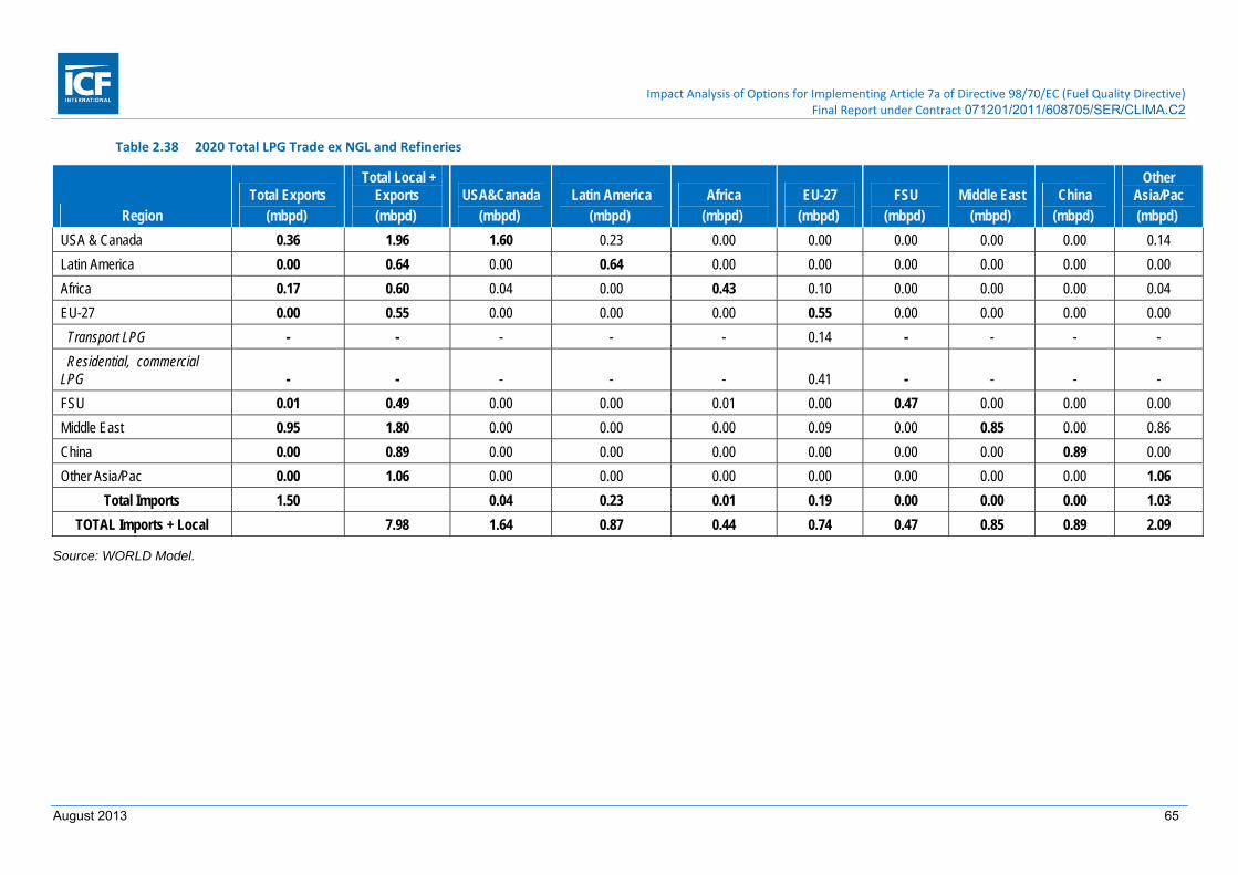
Impact Analysis of Options for Implementing Article 7a of Directive 98/70/EC (Fuel Quality Directive) Final Report under Contract 071201/2011/608705/SER/CLIMA.C2
August 2013 65
Table 2.38 2020 Total LPG Trade ex NGL and Refineries
Region Total Exports
(mbpd)
Total Local + Exports (mbpd)
USA&Canada (mbpd)
Latin America (mbpd)
Africa (mbpd)
EU-27 (mbpd)
FSU (mbpd)
Middle East (mbpd)
China (mbpd)
Other Asia/Pac (mbpd)
USA & Canada 0.36 1.96 1.60 0.23 0.00 0.00 0.00 0.00 0.00 0.14
Latin America 0.00 0.64 0.00 0.64 0.00 0.00 0.00 0.00 0.00 0.00
Africa 0.17 0.60 0.04 0.00 0.43 0.10 0.00 0.00 0.00 0.04
EU-27 0.00 0.55 0.00 0.00 0.00 0.55 0.00 0.00 0.00 0.00
Transport LPG - - - - - 0.14 - - - -
Residential, commercial LPG - - - - - 0.41 - - - -
FSU 0.01 0.49 0.00 0.00 0.01 0.00 0.47 0.00 0.00 0.00
Middle East 0.95 1.80 0.00 0.00 0.00 0.09 0.00 0.85 0.00 0.86
China 0.00 0.89 0.00 0.00 0.00 0.00 0.00 0.00 0.89 0.00
Other Asia/Pac 0.00 1.06 0.00 0.00 0.00 0.00 0.00 0.00 0.00 1.06
Total Imports 1.50 0.04 0.23 0.01 0.19 0.00 0.00 0.00 1.03
TOTAL Imports + Local 7.98 1.64 0.87 0.44 0.74 0.47 0.85 0.89 2.09
Source: WORLD Model.

Impact Analysis of Options for Implementing Article 7a of Directive 98/70/EC (Fuel Quality Directive) Final Report under Contract 071201/2011/608705/SER/CLIMA.C2
August 2013 66
Table 2.39 2020 Total Petrochemical Naphtha Trade (Fossil Fuel Only)
Region Total Exports
(mbpd)
Total Local + Exports (mbpd)
USA&Canada (mbpd)
Latin America (mbpd)
Africa (mbpd)
EU-27 (mbpd)
FSU (mbpd)
Middle East (mbpd)
China (mbpd)
Other Asia/Pac (mbpd)
USA & Canada 0.10 0.43 0.33 0.06 0.00 0.02 0.00 0.00 0.00 0.02
Latin America 0.00 0.33 0.00 0.33 0.00 0.00 0.00 0.00 0.00 0.00
Africa 0.09 0.13 0.00 0.00 0.04 0.09 0.00 0.00 0.00 0.00
EU-27 0.00 0.59 0.00 0.00 0.00 0.59 0.00 0.00 0.00 0.00
FSU 0.14 0.47 0.00 0.00 0.00 0.13 0.33 0.00 0.00 0.02
Middle East 0.96 1.06 0.00 0.00 0.00 0.00 0.00 0.10 0.00 0.96
China 0.00 1.68 0.00 0.00 0.00 0.00 0.00 0.00 1.68 0.00
Other Asia/Pac 0.00 2.14 0.00 0.00 0.00 0.00 0.00 0.00 0.00 2.14
Total Imports 1.29 0.00 0.06 0.00 0.23 0.00 0.00 0.00 0.99
TOTAL Imports + Local 6.83 0.33 0.39 0.04 0.82 0.33 0.10 1.68 3.14
Source: WORLD Model.

Impact Analysis of Options for Implementing Article 7a of Directive 98/70/EC (Fuel Quality Directive) Final Report under Contract 071201/2011/608705/SER/CLIMA.C2
August 2013 67
Table 2.40 2020 Total GTL ULS Distillate Trade
Region Total Exports
(mbpd)
Total Local + Exports (mbpd)
USA&Canada (mbpd)
Latin America (mbpd)
Africa (mbpd)
EU-27 (mbpd)
FSU (mbpd)
Middle East (mbpd)
China (mbpd)
Other Asia/Pac (mbpd)
USA & Canada 0.05 0.11 0.06 0.05 0.00 0.000 0.00 0.00 0.00 0.00
Latin America 0.00 0.01 0.00 0.01 0.00 0.001 0.00 0.00 0.00 0.00
Africa 0.03 0.06 0.00 0.00 0.03 0.029 0.00 0.00 0.00 0.00
EU-27 0.00 0.00 0.00 0.00 0.00 0.000 0.00 0.00 0.00 0.00
FSU 0.00 0.02 0.00 0.00 0.00 0.000 0.02 0.00 0.00 0.00
Middle East 0.13 0.25 0.00 0.00 0.00 0.000 0.00 0.12 0.00 0.13
China 0.00 0.00 0.00 0.00 0.00 0.000 0.00 0.00 0.00 0.00
Other Asia/Pac 0.00 0.04 0.00 0.00 0.00 0.000 0.00 0.00 0.00 0.04
Total Imports 0.21 0.00 0.05 0.00 0.029 0.00 0.00 0.00 0.13
TOTAL Imports + Local 0.49 0.06 0.06 0.03 0.030 0.02 0.12 0.00 0.17
Source: WORLD Model.

Impact Analysis of Options for Implementing Article 7a of Directive 98/70/EC (Fuel Quality Directive) Final Report under Contract 071201/2011/608705/SER/CLIMA.C2
August 2013 68
Table 2.41 2020 Total CTL ULS Distillate Liquids Trade
Region Total Exports
(mbpd)
Total Local + Exports (mbpd)
USA&Canada (mbpd)
Latin America (mbpd)
Africa (mbpd)
EU-27 (mbpd)
FSU (mbpd)
Middle East (mbpd)
China (mbpd)
Other Asia/Pac (mbpd)
USA & Canada 0.00 0.00 0.00 0.00 0.00 0.000 0.00 0.00 0.00 0.00
Latin America 0.00 0.00 0.00 0.00 0.00 0.000 0.00 0.00 0.00 0.00
Africa 0.04 0.15 0.00 0.00 0.11 0.000 0.00 0.00 0.00 0.04
EU-27 0.01 0.01 0.01 0.00 0.00 0.009 0.00 0.00 0.00 0.00
FSU 0.00 0.00 0.00 0.00 0.00 0.000 0.00 0.00 0.00 0.00
Middle East 0.00 0.00 0.00 0.00 0.00 0.000 0.00 0.00 0.00 0.00
China 0.06 0.21 0.00 0.00 0.00 0.000 0.00 0.00 0.15 0.06
Other Asia/Pac 0.00 0.07 0.00 0.00 0.00 0.000 0.00 0.00 0.00 0.07
Total Imports 0.11 0.01 0.00 0.00 0.000 0.00 0.00 0.00 0.10
TOTAL Imports + Local 0.44 0.01 0.00 0.11 0.009 0.00 0.00 0.15 0.17
Source: WORLD Model.

Impact Analysis of Options for Implementing Article 7a of Directive 98/70/EC (Fuel Quality Directive) Final Report under Contract 071201/2011/608705/SER/CLIMA.C2
August 2013 69
3 Baseline GHG Emissions and GHG Intensity (Task 1.2)
3.1 Introduction
This task is to develop an estimate of the baseline GHG emissions and GHG intensities associated with the baseline fuel projections from Task 1.1. The estimate is to be based on existing data from the literature review as well as values provided by the Commission. This task is also to consider a sensitivity where indirect land-use change (ILUC) emissions of biofuels are taken into account.
3.2 Scope
The GHG emissions attributable to the forecasted demand of various fuels17 is straightforward; it is the product of the carbon intensity (CI, as reported in grams of CO2 equivalents per unit of energy, gCO2(eq)/MJ) for each fuel and the corresponding energy consumed (measured in units of energy, MJ) of that fuel:
CIfuel fuelconsumed GHGemissionsfuel
For the baseline GHG emissions, we introduce uncertainty through both the CI and the fuel supply/demand.
3.3 Baseline GHG Emissions and GHG Intensity
As noted previously, the fuel projections developed for this analysis include petrol, diesel, LPG, CNG, electricity, and biofuels (distinguished here as ethanol or biodiesel). The carbon intensities for each of these fuels are shown in Tables 3.1 – 3.3 below, with the sources of data described in the following text.
Table 3.1 Default GHG Intensity for Fossil Fuels 2010
Feedstock source and process Fuel Type Upstream Unit GHG Intensity (gCO2eq/MJ)
Lifecycle Unit GHG Intensity (gCO2eq/MJ)
Conventional Crude Petrol 5.2 87.5
Conventional Crude Diesel or gasoil 5.3 89.1
Natural bitumen Petrol 24.7 107
Natural bitumen Diesel or gasoil 24.7 108.5
Oil shale Petrol 49 131.3
Oil shale Diesel or gasoil 49 133.7
Any fossil sources Liquefied Petroleum Gas
3.5 73.6
Any fossil sources Liquid or compressed natural gas
3.5 76.7
Coal converted to liquid fuel CTL petrol, diesel, or gasoil
100 172
Coal converted to liquid with Carbon Capture and Storage
CTL petrol, diesel, or gasoil
100 81
Natural gas converted to liquid fuel
GTL petrol, diesel, or gasoil
25 97
17 Only includes road vehicles and non-road mobile machinery. Marine and aviation fuels were not in the scope of this analysis.

Impact Analysis of Options for Implementing Article 7a of Directive 98/70/EC (Fuel Quality Directive) Final Report under Contract 071201/2011/608705/SER/CLIMA.C2
August 2013 70
Feedstock source and process Fuel Type Upstream Unit GHG Intensity (gCO2eq/MJ)
Lifecycle Unit GHG Intensity (gCO2eq/MJ)
Natural gas using steam reforming Hydrogen 3.5 82
Coal Hydrogen 100 190
Coal with Carbon Capture and Storage
Hydrogen 100 6
Waste plastic Petrol, diesel, or gasoil
0 86
Source: Annex I of the Commission’s 2011 proposal for a Directive laying down calculation methods and reporting requirements pursuant to Directive 98/70/EC, available at: http://ec.europa.eu/transparency/regcomitology/index.cfm?do=search.documentdetail&XOvfOQKYHt67nl0gDR9EQ0pDU4MfDGIJHglKuEmrBsRhxbx1TISJ2Mfg5DtxY23N
Table 3.2 GHG Intensity for Biofuels, ICF Study
Biofuel production pathway Estimated Average Direct Emissions
in 2020 (gCO2eq/MJ)
Corn (maize) 33
Sugar beet 27
Sugar cane 20
Wheat Process fuel not specified 50
2G ethanol - land using (farm wood) 17
2G ethanol - non-land using (wheat straw) 9
2G biodiesel - land using (farm wood DME) 5
2G biodiesel - non-land using (waste wood DME) 9
Waste 1st. Gen. diesel 9
FAME Palm oil 51
FAME Palm oil with methane capture 29
FAME Rapeseed 40
FAME Soybean 47
FAME Sunflower 32
Source: Provided by EC
Note: Assume FAME and HVO exhibit roughly same GHG emissions
Table 3.3 GHG Intensity for Biofuels, FQD Annex V
Biofuel and bioliquid production pathway
GHG Emissions for Cultivation, Processing,
Transport and Distribution (gCO2eq/MJ)
sugar beet ethanol 40
wheat ethanol (process fuel not specified) 70
wheat ethanol (lignite as process fuel in CHP plant) 70
wheat ethanol (natural gas as process fuel in conventional boiler) 55
wheat ethanol (natural gas as process fuel in CHP plant) 44
wheat ethanol (straw as process fuel in CHP plant) 26
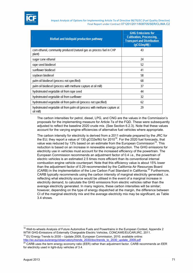
Impact Analysis of Options for Implementing Article 7a of Directive 98/70/EC (Fuel Quality Directive) Final Report under Contract 071201/2011/608705/SER/CLIMA.C2
August 2013 71
Biofuel and bioliquid production pathway
GHG Emissions for Cultivation, Processing,
Transport and Distribution (gCO2eq/MJ)
corn ethanol, community produced (natural gas as process fuel in CHP plant)
43
sugar cane ethanol 24
rape seed biodiesel 52
sunflower biodiesel 41
soybean biodiesel 58
palm oil biodiesel (process not specified) 68
palm oil biodiesel (process with methane capture at oil mill) 37
hydrotreated vegetable oil from rape seed 44
hydrotreated vegetable oil from sunflower 32
hydrotreated vegetable oil from palm oil (process not specified) 62
hydrotreated vegetable oil from palm oil (process with methane capture at oil mill)
29
The carbon intensities for petrol, diesel, LPG, and CNG are the values in the Commission’s proposals for the implementing measure for Article 7a of the FQD. These were subsequently adjusted to reflect the baseline 2020 crude mix. (See Section 6.2.3). Note that these values account for the varying engine efficiencies of alternative fuel vehicles where appropriate.
The carbon intensity for electricity is derived from a 2011 estimate prepared by the JRC for the EU; they report a value of 130 gCO2e/MJ for 201018. For the 2020 fuel forecasts, that value was reduced by 13% based on an estimate from the European Commission19. This reduction is based on an increase in renewable energy production. The GHG emissions for electricity use in vehicles must account for the increased efficiency of the powertrain. The European Commission recommends an adjustment factor of 0.4 i.e., the powertrain of electric vehicles is an estimated 2.5 times more efficient than its conventional internal combustion engine vehicle counterpart. Note that this efficiency value is about 15% lower than the adjustment factor of 0.29 recommended by the California Air Resources Board (CARB) in the implementation of the Low Carbon Fuel Standard in California.20 Furthermore, CARB typically recommends using the carbon intensity of marginal electricity generated, i.e. reflecting what electricity source would be utilised in the event of a marginal increase in electricity demand, to calculate the GHG emissions from electric vehicles rather than the average electricity generated. In many regions, these carbon intensities will be similar; however, depending on the type of energy dispatched at the margin, the difference between CI of the marginal electricity mix and the average electricity mix may be significant, as Table 3.4 shows.
18 Well-to-wheels Analysis of Future Automotive Fuels and Powertrains in the European Context, Appendix 2 WTW GHG-Emissions of Externally Chargeable Electric Vehicles, CONCAWE/EUCAR/JRC, 2011. 19 EU Energy Trends to 2030 – Update 2009, European Commission, 2010. available online: http://ec.europa.eu/energy/observatory/trends_2030/doc/trends_to_2030_update_2009.pdf 20 CARB uses the term energy economy ratio (EER) rather than adjustment factor. CARB recommends an EER for electricity used in light-duty vehicles of 3.4.

Impact Analysis of Options for Implementing Article 7a of Directive 98/70/EC (Fuel Quality Directive) Final Report under Contract 071201/2011/608705/SER/CLIMA.C2
August 2013 72
Table 3.4 Emissions intensity of displaced output21
Average emissions
intensity (tCO2/MWh) Low estimate of marginal
emissions intensity (tCO2/MWh)
High estimate of marginal emissions intensity
(tCO2/MWh)
Germany 0.50 0.53 (natural gas) 1.09 (lignite)
United Kingdom
0.452 0.3939 (combined-cycle gas
turbine generation)
0.6900 (Hawkes, 2010 – regression analysis on observed
dispatch of generators for the period 2002-9)
Source: Australian Productivity Commission, 2011
The carbon intensities for the biofuels derived from various feedstocks were provided by the European Commission (via the Joint Research Centre). These values include data on the estimated direct GHG balance of different biofuel pathways by 2020 based on expected improvements due to the implementation of current policies, such as reductions in fertiliser emissions (covered by the EU Emissions Trading System), under a business as usual scenario. These values do not include GHG emissions attributable to indirect land use change.
The GHG emissions for the baseline scenario are shown below in Table 3.5. We estimate total GHG emissions of 911.85 million metric tons (MMT) for the mix of transportation fuels forecasted in 2020, yielding a net carbon intensity of 83.76 gCO2e/MJ, a 5.1% reduction from the 2010 baseline of 88.3 gCO2e/MJ. The GHG intensity shown in the far right column is the GHG emissions of the transportation fuel divided by the sum of the forecasted energy demand in the transportation sector; the sum of these values yields the net carbon intensity. In ICF’s baseline forecast, petrol is 11.7 vol% ethanol, and diesel is 10.5 vol% biodiesel.
Petrol and diesel are forecasted to make up about 26% and 67% of the GHG emissions of the transportation fuel mix, respectively, and meet the majority of forecasted energy demand in the transportation sector. However, the increased demand for alternative fuels, including a small increase in LPG, CNG, and electricity, and significant increases in biofuel consumption as petrol and diesel substitutes, yield sufficient reductions to comply with the FQD. The goal of a 6% reduction in GHG emissions intensity from the 2010 baseline is not achieved given the projected crude slate and amount of MS biofuels in the baseline.
21 Productivity Commission. 2011. “Carbon Emission Policies in Key Economies.” Appendix L. Available online at : http://www.pc.gov.au/projects/study/carbon-prices/report
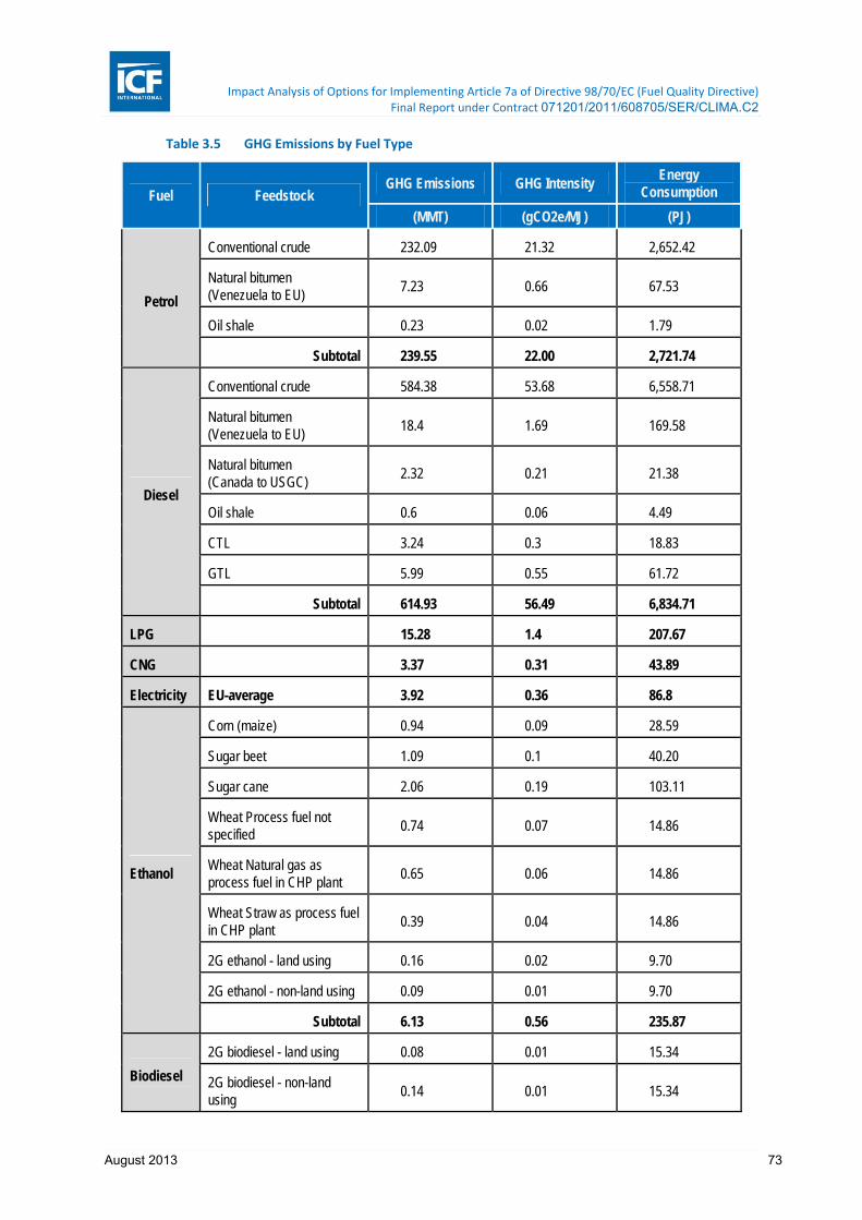
Impact Analysis of Options for Implementing Article 7a of Directive 98/70/EC (Fuel Quality Directive) Final Report under Contract 071201/2011/608705/SER/CLIMA.C2
August 2013 73
Table 3.5 GHG Emissions by Fuel Type
Fuel Feedstock GHG Emissions GHG Intensity
Energy Consumption
(MMT) (gCO2e/MJ) (PJ)
Petrol
Conventional crude 232.09 21.32 2,652.42
Natural bitumen (Venezuela to EU)
7.23 0.66 67.53
Oil shale 0.23 0.02 1.79
Subtotal 239.55 22.00 2,721.74
Diesel
Conventional crude 584.38 53.68 6,558.71
Natural bitumen (Venezuela to EU)
18.4 1.69 169.58
Natural bitumen (Canada to USGC)
2.32 0.21 21.38
Oil shale 0.6 0.06 4.49
CTL 3.24 0.3 18.83
GTL 5.99 0.55 61.72
Subtotal 614.93 56.49 6,834.71
LPG 15.28 1.4 207.67
CNG 3.37 0.31 43.89
Electricity EU-average 3.92 0.36 86.8
Ethanol
Corn (maize) 0.94 0.09 28.59
Sugar beet 1.09 0.1 40.20
Sugar cane 2.06 0.19 103.11
Wheat Process fuel not specified
0.74 0.07 14.86
Wheat Natural gas as process fuel in CHP plant
0.65 0.06 14.86
Wheat Straw as process fuel in CHP plant
0.39 0.04 14.86
2G ethanol - land using 0.16 0.02 9.70
2G ethanol - non-land using 0.09 0.01 9.70
Subtotal 6.13 0.56 235.87
Biodiesel
2G biodiesel - land using 0.08 0.01 15.34
2G biodiesel - non-land using
0.14 0.01 15.34

Impact Analysis of Options for Implementing Article 7a of Directive 98/70/EC (Fuel Quality Directive) Final Report under Contract 071201/2011/608705/SER/CLIMA.C2
August 2013 74
Fuel Feedstock GHG Emissions GHG Intensity
Energy Consumption
(MMT) (gCO2e/MJ) (PJ)
Waste 1st. Gen. Diesel 0.28 0.03 30.67
Palm oil 4.19 0.38 82.18
Palm oil with methane capture
2.38 0.22 82.05
Rapeseed 15.41 1.41 385.29
Soybean 4.93 0.45 104.98
Sunflower 1.27 0.12 39.66
Subtotal 28.68 2.63 755.50
Total 911.85 83.76 10,886.17
Note that the GHG intensity in the above table has been calculated based on the EC’s default values as published. In Tasks 2 and 3 revised calculations have been used as discussed in the relevant sections.
3.4 Sensitivity Analysis including ILUC Emissions
3.4.1 Introduction to GHG Emissions from ILUC
The GHG emissions attributable to the baseline fuel projections were calculated based on the product of the energy demand for each fuel and the corresponding carbon intensity, as discussed in more detail previously. The carbon intensity values used previously did not account for the GHG emissions from indirect land use change (ILUC). ILUC emissions arise from the unintended consequence of land shifts resulting from the expansion of croplands for biofuels derived from feedstocks that are cultivated on land. There is still considerable uncertainty regarding the models used to estimate the GHG emissions resulting from ILUC; however, the field of study has evolved rapidly and uncertainties are narrowing.
For the purposes of this sensitivity analysis, ICF first considered the impacts of including ILUC emissions in the fuel projections in the reference forecast to 2020. The GHG emission intensities of biofuels from various feedstocks after accounting for corresponding ILUC emissions are shown in the table below. The last column lists the per cent contribution to biofuel demand on an energy basis in the reference forecast in 2020.

Impact Analysis of Options for Implementing Article 7a of Directive 98/70/EC (Fuel Quality Directive) Final Report under Contract 071201/2011/608705/SER/CLIMA.C2
August 2013 75
Table 3.6 Total Biofuel GHG Intensities Including ILUC
Biofuel Production Pathway GHG intensity (g CO2e/MJ) % biofuels
energy WTW ILUC1 Total
Ethanol Corn (maize) 33 10 43 2.9%
Sugar beet 27 7 34 4.1%
Sugar cane 20 15 35 10.4%
Wheat, Process fuel not specified 50 14 64 1.5%
Wheat, Natural gas as process fuel in CHP plant 44 14 58 1.5%
Wheat, Straw as process fuel in CHP plant 26 14 40 1.5%
2G ethanol - land using 17 152 32 1.0%
2G ethanol - non-land using 9 -- 9 1.0%
Biodiesel 2G biodiesel - land using 5 152 20 1.5%
2G biodiesel - non-land using 9 -- 9 1.5%
Waste oils 9 -- 9 3.1%
Palm oil 51 54 105 8.3%
Palm oil with methane capture 29 54 83 8.3%
Rapeseed 40 55 94 38.9%
Soybean 47 56 103 10.6%
Sunflower 32 54 86 4.0% 1 http://trade.ec.europa.eu/doclib/docs/2011/october/tradoc_148289.pdf
2 Estimates for ILUC from land-using 2G ethanol and biodiesel were provided by the European Commission. Although the specific ILUC emissions associated with typical land using second generation biofuels were not modelled by IFPRI, these are assumed to be at the same level as for sugarcane for this assessment (i.e. high yielding crop worth no land saving co-products).
As shown in Table 3.7below, after accounting for ILUC, the higher GHG intensities of biofuels result in a significant increase of the GHG intensity of the fuel mix in 2020 compared to the baseline fuel projections outlined previously. This is largely unsurprising considering the significant ILUC emissions attributable to biofuels produced from feedstocks such as rapeseed, soybean, palm oil, and sunflower. These biodiesel feedstocks alone account for 70% of the energy consumed as biofuels in the transportation sector. Although the GHG intensities of bioethanol from feedstocks such as maize or sugarcane increased significantly after including ILUC emissions, the increase was not nearly as significant as biodiesel feedstocks and their contribution to the overall biofuel energy demand is about half of the demand of biodiesel feedstocks.
Table 3.7 GHG Intensity of Baseline Fuel Projections in 2020
GHG Intensity (gCO2eq/MJ)
FQD Target w/o ILUC w/ ILUC
Baseline Projection 83.00 83.76 87.17

Impact Analysis of Options for Implementing Article 7a of Directive 98/70/EC (Fuel Quality Directive) Final Report under Contract 071201/2011/608705/SER/CLIMA.C2
August 2013 76
3.4.1 Scenario to Demonstrate Sensitivity
To demonstrate the sensitivity of the baseline fuel projections to ILUC, ICF was directed by the European Commission to assume that suppliers would no longer blend biodiesel from feedstocks with GHG intensities that do not provide at least a 50% GHG reduction benefit compared to petrol or diesel.
The impact of incorporating ILUC is significant: Two bioethanol pathways and five biodiesel pathways were eliminated. Two pathways for bioethanol from wheat were eliminated, including the one in which the process fuel is not specified and another in which the process fuel is natural gas in a CHP plant. The biodiesel pathways that were eliminated from consideration in the modified projections incorporating ILUC included: palm oil (with and without methane capture), rapeseed, soybean, and sunflower. These fuels represented 724 PJ of the 992 PJ of demand for biofuels; the demand from the biodiesel sector is most significant, with about 92% of forecasted biodiesel demand in 2020 eliminated from consideration. Displacing this bioethanol and biodiesel demand with fossil petrol and diesel demand at 87.5 gCO2/MJ and 89.1 gCO2/MJ will require an additional 45.3 Mt of CO2 abatement in 2020.
See Section 4.3 for details of GHG reduction measures and their costs.
The revised emissions for the fuel forecast out to 2020 after displacing the selected biodiesel pathways are shown in the table below.

Impact Analysis of Options for Implementing Article 7a of Directive 98/70/EC (Fuel Quality Directive) Final Report under Contract 071201/2011/608705/SER/CLIMA.C2
August 2013 77
Table 3.8 GHG Emissions and Intensity for the ILUC Sensitivity Scenario
Fuel Feedstock GHG Emissions GHG Intensity Energy Demand
(MMT) (gCO2e/MJ) PJ
Petrol
Conventional crude 234.69 21.56 2682.14
Natural bitumen (Venezuela to EU) 7.23 0.66 67.53
Oil shale 0.23 0.02 1.79
Diesel
Conventional crude 646.23 59.36 7,252.86
Natural bitumen (Venezuela to EU) 18.4 1.69 169.58
Natural bitumen (Canada to USGC) 2.32 0.21 21.38
Oil shale 0.60 0.06 4.49
CTL 3.24 0.30 18.83
GTL 5.99 0.55 61.72
LPG n/a 15.28 1.40 207.67
CNG n/a 3.37 0.31 43.89
Electricity EU-average 3.92 0.36 86.80
Ethanol
Corn (maize) 1.23 0.11 28.59
Sugar beet 1.37 0.13 40.20
Sugar cane 3.40 0.31 103.11
Wheat (Process fuel not specified) Displaced
Wheat (NG as process fuel, w/ CHP) Displaced
Wheat (Straw as process fuel, w/ CHP) 0.59 0.09 14.86
2G ethanol - land using 0.15 0.01 9.70
2G ethanol - non-land using 0.09 0.01 9.70
sub-total 6.83 0.63 206.15
Biodiesel
2G biodiesel - land using 0.23 0.02 15.34
2G biodiesel - non-land using 0.14 0.01 15.34
Waste 1st. Gen Diesel (2G) 0.28 0.03 30.67
Palm oil Displaced
Palm oil with methane capture Displaced
Rapeseed Displaced
Soybean Displaced
Sunflower Displaced
sub-total 0.64 0.06 61.35
Total 948.98 87.17 10,886.17
Although the implementation of the methane flare reduction projects will help comply with the FQD, the revised scenario does not comply with the RED because such a large volume of biodiesel was displaced. Under the revised ILUC sensitivity scenario, approximately 5.1% of energy in the transport sector is attributable to biofuels, compared to the 10% renewable target.
Impact Analysis of Options for Implementing Article 7a of Directive 98/70/EC (Fuel Quality Directive) Final Report under Contract 071201/2011/608705/SER/CLIMA.C2
August 2013 78
4 Costs of the Baseline (Task 1.3)
4.1 Introduction
This task is to develop the costs of the changes in energy demand for transport fuels between 2010 and 2020, based on the baseline projections developed in Task 1.1, and including consideration for the ILUC sensitivity.
4.2 Scope
The costs of the baseline fuel projections are dependent on the product of two variables: the marginal abatement cost (MAC) of each strategy reported on a €/tonne (€/t) basis and the amount of reductions achieved in tonnes: Although a simple calculation, there is considerable uncertainty and complexity associated with the former variable i.e., the abatement costs associated with the reduction of carbon emissions.
Marginal abatement costs for GHG reductions are a function of the GHG reduction potential of a strategy. For transport fuels, the GHG reduction potential is a function of factors such as supply constraints from feedstock availability and distribution infrastructure constraints. The costs22 associated with each strategy are typically assessed using a discounted cash flow whereby costs are allocated over a given period.
Due to resource constraints and project scope, the marginal abatement costs for this study are largely taken from those available in the literature, with any modifications noted where appropriate. One of the most significant challenges for this study is distinguishing between strategies that would have been implemented without the FQD in place and those that will be implemented to comply with the FQD. The most relevant strategy, for instance, that is not a result of the FQD is the CO2 emission standards for light-duty vehicles, including cars and fleets. For cars in 2020, the current mandatory target is 95 g of CO2 per kilometre (gCO2/km), down from an average of about 135.7 gCO2/km in 2011. For vans, the mandatory target is 147 gCO2/km, down from 181.4 gCO2/km in 2010.23
In the following sub-sections we review the GHG reductions attributable to the various fuels forecasted in the baseline projections, after accounting for the reductions attributable to vehicle CO2 standards. Following that, we review a subset of the available literature for MACs of these various strategies.
Note that this section does not consider administrative costs, as increments in these costs are not assumed in the baseline.
4.3 GHG Reductions of Strategies in the Baseline Projections
Note that we have extracted the estimated GHG reductions attributable to CO2 standards for light-duty vehicles to ensure that our analysis focuses on the strategies included in the baseline fuel projections that will be modified in subsequent tasks.
In the following sections we review the initial demand for various alternative transport fuels in 2010 and compare that against 2020. Based on the changes in energy demand out to 2020, we estimate the GHG emissions reduction, based on the differential between the alternative transport fuel and the petroleum-based fuel that it displaces.
22 Including one-off capital costs and recurring annual costs and / or savings 23 Additional information available online at: http://ec.europa.eu/clima/policies/transport/vehicles/index_en.htm

Impact Analysis of Options for Implementing Article 7a of Directive 98/70/EC (Fuel Quality Directive) Final Report under Contract 071201/2011/608705/SER/CLIMA.C2
August 2013 79
Table 4.1 Change in Energy Demand for Transport Fuels, 2010‐2020
Strategy
Energy Demand
(PJ)
2010 2020 Delta
Bioethanol 90 236 146
corn 29 29 0
sugar beet 24 40 16
sugar cane 9 103 94
wheat 28 45 17
2G ethanol 0 19 19
Biodiesel 414 755 342
palm oil 54 164 110
rapeseed 234 385 151
soybean 89 105 16
sunflower 6 40 34
waste oils 31 31 0
2G biodiesel 0 31 31
Electricity 1 87 86
CNG 40 44 4
LPG 189 208 19
4.3.2 Bioethanol
Based on projections provided by the EC for 2020, there is a significant increase between 2010 and 2020 of bioethanol consumption, representing about a 160% increase. This forecasted demand for ethanol yields a blend of 11.7% by volume with petrol. Based on EC projections, more than 40% of bioethanol demands will be met by sugarcane ethanol, with wheat, corn, and sugar beet representing a combined 48% of the demand for bioethanol, by energy. The EC also projects that second generation bioethanol will represent 8% of total bioethanol demand by 2020.
4.3.3 Biodiesel
The EC projects that biodiesel demand will increase by about 83% by 2020, yielding a 10.5% blend by volume with diesel. Biodiesel produced from rapeseed represents 51% of the forecasted market in 2020, with palm oil and soybean capturing an estimated 36% of the market. Biodiesel from waste, second generation biodiesel, and biodiesel derived from sunflower are forecast to represent about 4%, 5% and 4% of the market, respectively.
4.3.4 Electricity
Based on ICF’s fuel projections (in Section 2, Task 1.1), electricity consumption in the transportation sector will increase significantly by 2020, with about 113 PJ of energy. This increase is attributable to electricity using in light-duty plug-in electric vehicles, including plug-in hybrid electric vehicle (PHEV) and battery electric vehicle (BEV) configurations.
4.3.5 CNG and LPG
ICF’s forecast yields a 10% increase for CNG and LPG consumption out to 2020.
Impact Analysis of Options for Implementing Article 7a of Directive 98/70/EC (Fuel Quality Directive) Final Report under Contract 071201/2011/608705/SER/CLIMA.C2
August 2013 80
4.4 Review of Marginal Abatement Costs
Marginal abatement costs express the cost of a reduction measure on a € per metric tonne of CO2 equivalent basis (€/tCO2). There are a variety of parameters and assumptions that impact reported abatement costs (or cost-effectiveness) of GHG reduction measures, including the cost of the baseline technology, the discount rate used, the assumed lifetime, and anticipated technological change or improvement. In other words, there is plenty of room for uncertainty. To estimate the costs associated with the baseline fuel projections, ICF has opted to use a range of abatement costs across all technologies based on values reported in the literature – in some cases, ICF modified abatement costs when deemed necessary.
The primary challenge of assigning an abatement cost to many of the GHG reduction measures included in the fuel projections is capturing technological improvement. For instance, as noted previously, our fuel projections indicate a significant increase in electricity consumption from PHEVs and BEVs (combined) while also introducing significant quantities of second generation biofuels. In both of these cases, there are many technological improvements and cost reductions that will be required to make these strategies viable. To the extent feasible, ICF has communicated the assumptions regarding each GHG reduction measure.
The costs reported are for the absolute costs of the alternative fuels: We opted to present costs as absolutes to reduce the dependency on assumptions about forecasted fuel pricing. To determine the incremental costs (as opposed to absolute costs) of the various strategies compared to fossil fuels is a simple exercise with the absolute costs already estimated; however, this calculation is significantly dependent on the assumed price of petrol or diesel or in the case of a strategy that requires a new vehicle (e.g., electricity, CNG, and LPG), the price of the conventional vehicle being displaced. Note that the cost-benefit analysis in Tasks 2 and 3 will focus on incremental costs of GHG reduction measures, taking into account any savings from displaced fuels.
In the following sections we highlight the range of marginal abatement costs available in the literature associated with various alternative transport fuels. The ranges of marginal abatement costs of the options are shown in Table 4.3 below; the options are grouped from left to right as bioethanol, biodiesel, electricity, CNG, LPG, and methane flare reductions. Note that in the case of biofuels, we distinguish between feedstocks to the extent possible. All costs are presented in €2010 unless otherwise noted. The reports used to generate this plot are discussed in more detail in subsequent sections.

Impact Analysis of Options for Implementing Article 7a of Directive 98/70/EC (Fuel Quality Directive) Final Report under Contract 071201/2011/608705/SER/CLIMA.C2
August 2013 81
Table 4.2 Range of MACs for Strategies in the Baseline Fuel Projections, 2020
4.4.2 Bioethanol
There is a broad range of marginal abatement costs reported in the literature for bioethanol; however, the literature does not provide the details used to estimate the marginal abatement costs of biofuels e.g., a detailed breakdown of the cost elements and assumptions used to develop overall costs. The marginal costs of production for biofuels can be characterised as follows:
Marginalcost C C C C C ,
Cost element Description
Feedstock Cost of the feedstock which varies by feedstock type
Transport Cost of transporting the feedstock to the biofuel production facility
Operations Cost of operating a biofuel production facility including energy use, water use, and other resource costs
Installed capacity Amortized cost of installing biofuel production facilities
By-products The by-products of bioethanol production often have value in other markets; these lower the overall marginal cost of producing some biofuels.
For each of these cost elements, the range of what has been reported in the literature has been updated to reflect more recent biofuel feedstock price outlooks, modified outlooks for the price of oil, and the most recent data regarding operating efficiencies.
0
50
100
150
200
250
300
350
400
450
500
550
600
650
700
corn
sugarbeet
sugarcane
wheat
2G EtOH
palm oil
rapeseed
soybean
sunflower
waste oil
2G BD
electricity
CNG
LPG
flare reduction
Marginal Abatem
ent Cost (€/tonne)

Impact Analysis of Options for Implementing Article 7a of Directive 98/70/EC (Fuel Quality Directive) Final Report under Contract 071201/2011/608705/SER/CLIMA.C2
August 2013 82
Table 4.3 Unit costs for selected bioethanol feedstocks
Bioethanol Feedstock
Cost element (€/GJ)
Feedstock Transport Operations/
Capacity Co-product Total
Corn 23 c 6.1 c 2.9 c 12-20 a
27 c
Sugar Beet 12-14 a 6.4 c 2.0 a
4.8 c
12-24 a
19 c
Sugarcane
4.5 c
28 d
7.5 e
4.1 c
5.5 d
4.7 e
4.6 d
6.4 e
15 a
12 c
18.6 e
Wheat 13-15 a
26 d
5.5 d 6.1 c
2.6 d
3 a
3.5 c
3.7 d
12-23 a
32 c
31 e
2G Ethanol
10-13 a
11 c
11 d
5.5 d 15-16 a
7.5 c
20.3 d
-5.8 d
25-28 a
18 c
31 d
Bioethanol 19 b
[a] Szabo et al.. Assessment of the GHG reduction potential and cost curves resulting from fuel substitution possibilities
[b] Estimating the Cost-Effectiveness of Biofuels, Defra, 2008
[c] Committee on Climate Change, UK
[d] Data from COWI’s Danish model for alternative fuels, the A-D Model.
[e] Cargo et al. Competitiveness of Brazilian Sugarcane Ethanol Compared to US Corn Ethanol, 2010.
The critical assumptions for many of these studies, and other references, are not readily available in the reports prepared. For instance, McKinsey prepared a report on behalf of the BDI Initativ – Business for Climate in Germany. In the report, the discussion regarding the abatement costs for bioethanol is limited to the following:
… based on targets discussed by the German government, [biofuels] would contribute an additional potential of 14 Mt CO2e for passenger cars and trucks. In the case of petrol, potentials can be achieved by using first generation ethanol, imports from Brazil, and a share of second-generation ethanol beginning in 2015. A calculation based on current import tariffs of 19 cent/litre leads to abatement costs for 2020 from EUR 130/t CO2e to EUR 320/t CO2e.
The McKinsey study, like others reviewed here, does not include information regarding the assumptions embedded in the range e.g., transport costs, production costs, or technology improvements. Furthermore, studies like the review prepared by the Economics group at Defra (2008) present summaries of the bundled production costs and report negative cost-effectiveness values. In this case, negative cost-effectiveness values for bioethanol are reflective of a calculation performed relative to some reference fuel; however, it is unclear what the reference fuel (specifically, the feedstock of ethanol used) is in the report.
The costs of discount rates and handling taxes as transfers was discussed in detail in one study prepared for the UK Committee on Climate Change. In that report, the authors write that the net present value of strategies to reduce GHG emissions in the transport sector are calculated using discount rates that are differentiated in the case of a social MAC curve and

Impact Analysis of Options for Implementing Article 7a of Directive 98/70/EC (Fuel Quality Directive) Final Report under Contract 071201/2011/608705/SER/CLIMA.C2
August 2013 83
a private MAC curve. In the former, they use a social discount rate of 3.5% and treated taxes as transfers; in the latter, they used a private discount rate of about 7% and included a cost of about 35 cents per litre.
Based on ICFs’ literature review and own analyses, the feedstock type, feedstock costs, and distribution constraints are the major drivers for higher abatement costs.
Based on ICF’s review of the literature and internal analyses, the following abatement costs are presented in €2010 for the year 2020; where appropriate (e.g. investments required in infrastructure), a discount rate of 7% was used. For bioethanol that was assumed to be imported e.g., sugarcane ethanol, we included a duty rate. For sugarcane ethanol, this is €10.2/hl.
As noted previously, much of the literature reviewed did not include critical assumptions regarding discount rates and tax subsidies. To the extent feasible, ICF attempted to duplicate calculations performed where limited information were available. In the cases that ICF was able to duplicate estimates with a high level of confidence, these studies were given higher weighting in the results presented below. Neither subsidies nor tax rates were included in our analysis.
■ Corn: Corn-based ethanol has been an issue of much study, mostly in the USA because it is effectively the exclusive pathway for bioethanol production today in the USA, blended with petrol in over 90% of the US market, generally at levels up to 10% by volume. Recent estimates24 indicate that there is wide variation even among operating production plants. Corn is being increasingly planted in parts of Europe and we report marginal abatement costs in the range of €223-364/t.
■ Sugarcane: There is a considerable amount of conflicting literature regarding the abatement costs of bioethanol derived from Brazilian sugarcane. We use an average unit production cost from most recent reports of €15/GJ, which includes feedstock production, transport, production, and distribution. One of the main factors impacting the marginal abatement cost of sugarcane ethanol in the EU is the import tariff; we include the 10.2 cents/per litre tariff on imported sugarcane. The literature that was reviewed for this report maintained this tariff in the estimates of unit costs for sugarcane ethanol until at least 2020. Before the tariff, sugarcane has a range of abatement costs of €178-276/t. The tariff, however, adds €71/t.
■ Sugar beet and wheat: Sugar beets and wheat are both produced in the EU. Sugar beet has the potential to be a high yield and environmentally friendly feedstock for biofuels with relatively low production costs. Sugar beet can be produced in Europe, however, it requires specific conditions e.g., "rich soil" and thereby competes with high quality food production. Due to the limited conditions under which it thrives, the main driver for the cost of sugar beet is likely to be the feedstock rather than the refining or transport. We report a range of €205-394/t for sugar beets and €326-608/t for wheat.
■ 2G ethanol: The primary driver for the costs of 2G ethanol in 2020 will be technological maturity. Today, there is limited commercial scale production of bioethanol e.g., Mossi & Ghisolfi Group’s 50 million litre per year facility in Crescentino in north-western Italy. Since there is limited commercial scale quantities of so-called second generation bioethanol produced today, it is difficult to estimate the potential abatement costs in 2020. McKinsey estimates that by 2030, 2G biofuels such as bioethanol will have a significant negative abatement cost (i.e., yield net savings to society via introduction of the measure) of roughly -€95/t.25 This abatement cost for 2020, however, is highly unlikely; we report a range of abatement costs for 2G bioethanol of €244-411/t
24 Wamisho, K. The Shadow Price of GHG Reduction in Corn Ethanol Plants, presented at 2012 AAEA Annual Meeting, Seattle, Washington, August 12-14, 2012. 25 Enkvist, P-A; Dinkel, J., and Lin, C. Impact of the financial crisis on carbon economics, v2.1 of the Global GHG Abatement Cost Curve, McKinsey & Co., 2010.

Impact Analysis of Options for Implementing Article 7a of Directive 98/70/EC (Fuel Quality Directive) Final Report under Contract 071201/2011/608705/SER/CLIMA.C2
August 2013 84
4.4.3 Biodiesel
We review the same cost elements discussed for bioethanol as part of the unit costs for biodiesel from various feedstocks, as shown in the table below.
Table 4.4 Unit costs for selected biodiesel feedstocks
Biodiesel Feedstock
Cost element (€/GJ)
Feedstock Transport Operations/
Capacity Co-product Total
Rapeseed
27.9 c
31.8 c
22 d
3.8 d 2.1 c
4.9 d
1.4 c
11.9 d
11.8 – 17 a
22.3 c
32.6 c
19 d
Sunflower 20-23 e 1-4 e 3.3 c
2.1 c 24.2 – 32.5 e
Soybean 78.9 c
17.8 c
3.3 c
2.1 c
43.7 c
1.4 c
38.5 c
18.6 c
Palm Oil 19.7 c
21.7 d 3.8 d
2.1 c
4.7 d 1.4 c
20.4 c
29.5 d
Recycled Oils
Animal Fats 10.7-16.5 e 3.0 e 1.2 e 14.5-20.1 e
2G Biodiesel
10-13 a
10.0 c
9.6 c
14.5 d
6.7
15-16 a
3.5 c
6.1 c
7.4 d
1.4 c
25-28 a
12.1 c
15.7 c
28.6d
[a] Szabo et al.. Assessment of the GHG reduction potential and cost curves resulting from fuel substitution possibilities
[c] Committee on Climate Change, UK
[d] Data from COWI’s Danish model for alternative fuels, the A-D Model.
[e] ICF analysis.
Similar to bioethanol, there is a broad range of marginal abatement costs reported in the literature for biodiesel. Based on ICFs’ literature review and own analyses, the feedstock type, feedstock costs, and distribution constraints are the major drivers for higher abatement costs. Because biodiesel is produced via processing of vegetable oils, the feedstock type determines the oil yield from the seed or crop. As a result, the crop yield and the oil yield contribute significantly to the cost ranges reported for biodiesel feedstock, particularly as a function of feedstock origin.
Based on ICF’s review of the literature and internal analyses, the following abatement costs are presented in €2010 for the year 2020; where appropriate (e.g. investments required in infrastructure), a discount rate of 7% was used. For biofuels that were assumed to be imported e.g., biodiesel from palm oil, include duty rates. We assumed shipments of B96.5-B100, which are subject to a duty of 6.5%.
As noted previously, much of the literature reviewed did not include critical assumptions regarding discount rates and tax subsidies. To the extent feasible, ICF attempted to duplicate calculations performed where limited information were available. In the cases that ICF was able to duplicate estimates with a high level of confidence, these studies were
Impact Analysis of Options for Implementing Article 7a of Directive 98/70/EC (Fuel Quality Directive) Final Report under Contract 071201/2011/608705/SER/CLIMA.C2
August 2013 85
given higher weighting in the results presented below. Neither subsidies nor tax rates were included in our analysis.
■ Palm oil: Palm oil is generally sourced from Southeast Asia and has oil yields as high as 6,000 litres per hectare (l/ha), making the amortized cost of investment into biofuel production more attractive. Based on data provided by COWI and data from the report to the UK Committee on Climate change, we estimate a range of biodiesel derived from palm oil of €415-601/t.26 It is also worth noting that there are acute sustainability concerns with palm oil, which will impact the viability of palm derived biodiesel moving forward.
■ Rapeseed and sunflower oil: Both rapeseed and sunflower seeds are produced in the EU-27 and have similar oil yields of about 1,000-1,200 l/ha. There is a broad range of estimates available in the literature for the abatement costs of biodiesel derived from rapeseed and sunflower, largely depending on the country of origin of the feedstock. We report marginal abatement costs range of €387-664/t27 for rapeseed and €423-569/t for sunflower.
■ Soybean oil: Soybean oil has a lower yield of about 500 l/ha; soy is currently the predominant feedstock for biodiesel production in the US and Argentina; both countries have exported considerably quantities of soybean biodiesel to the EU. Similarly, soy oil is a feedstock for domestic production and soy is also a significant export to the EU-27. We report marginal abatement costs range of €442-594/t.
■ Waste oils: Recycled vegetable oils and animal fats are an increasingly popular feedstock in the EU with projected growth of 33% and 20% in the near-term future, respectively. The introduction of a cap on the percentage of biofuels that can come from crop-based biofuels to meet the 10% renewable energy target in the RED will aid in the deployment of biodiesel from waste oils. Based on ICF estimates, abatement costs for biodiesel derived from waste oils ranges from €181-251/t
■ 2G Biodiesel: The same issues identified previously for 2G bioethanol apply to biodiesel: The current market outlook for commercial production potential of 2G biodiesel in 2020 will yield abatement costs in the range outlined of €305-341/t.
The MAC curve for biofuels – including the feedstocks discussed in the previous subsections – is shown below. For illustrative purposes we have separated the MAC curves for bioethanol and biodiesel. Furthermore, we have shown the MAC for bioethanol from sugarcane ethanol as a straight line – representing the average unit cost of production. The lower and upper dashed lines represent the MAC of sugarcane ethanol without and with the current tariff, respectively. This is important to note because the production of ethanol in the EU-27 is not as cost competitive in a carbon-constrained market (e.g., under the FQD) without the tariff.
26 Deconti, M. Estimating the Cost-Effectiveness of Biofuels, Defra, April 2008. 27 McKinsey and Co., Costs and Potentials of Greenhouse Gas Abatement in Germany, 2007

Impact Analysis of Options for Implementing Article 7a of Directive 98/70/EC (Fuel Quality Directive) Final Report under Contract 071201/2011/608705/SER/CLIMA.C2
August 2013 86
Table 4.5 Marginal abatement costs of biofuels in the EU‐27
4.4.4 Electricity
ICF estimates an abatement cost for electricity used in electric vehicles at €300-700/t by 2020. This range is largely a function of parameters such as vehicle costs, assumed level of vehicle subsidy, and the vehicle miles travelled (VMT). The range reported includes the costs of a compact car driving nearly 11,000 km/yr, a light-duty sedan that is driving nearly 13,000 km/yr, and a compact van that drives about 23,000 km/yr. Although the vehicle pricing differential is similar across these vehicle classes, the additional mileage travelled in the compact van yields considerable fuel savings over the life of the vehicle, resulting in a much more attractive abatement cost. The low end of the abatement costs reported for electricity assume a battery size about 50-75% lower capacity (as measured in kWh) for PHEVs compared to BEVs. We also assume a subsidy of up to €5,000 per vehicle is available. The range can also vary significantly depending on the price of electricity, and electricity prices can vary considerably across the EU. The vehicle price is driven largely by battery pricing. For the purposes of our analysis, we assume a 30% decrease in battery prices (on a per kWh basis) by 2020. These estimates are based on a recent discussion paper for the OECD regarding electric vehicles.28 Furthermore, recent research conducted by ICF on behalf of the EC also confirms the estimated 30% reduction in battery prices out to 2020.29
4.4.5 CNG and LPG
ICF estimates abatement costs for CNG from €340-497/t, depending most significantly on the type of vehicle (passenger car vs. truck), the anticipated number of refuelling stations required, and the price differential between natural gas and oil. A large price differential between natural gas and petroleum-derived fuels has persisted in the USA for the last 18 months, largely driven by increased reserves of so-called shale gas. As recently as 2009, there was no shale gas production in Europe. If shale gas reserves in the EU-27 prove to be
28 Crist, P. Electric Vehicles Revisited – Costs, Subsidies, and Prospects, Discussion Paper, OECD, May 2012. 29 Duleep, KG., et al., Impacts of Electric Vehicle: Assessment of electric vehicle and battery technology. April 2011, ICF International and Ecologic Institute.
0
100
200
300
400
500
600
700
0 10 20 30 40 50 60 70 80
Abatem
ent Cost (€/ton)
Abatement Potential (MMT)
Biodiesel
Bioethanol
Sugarcane ethanol

Impact Analysis of Options for Implementing Article 7a of Directive 98/70/EC (Fuel Quality Directive) Final Report under Contract 071201/2011/608705/SER/CLIMA.C2
August 2013 87
sufficient to sustain a significant price differential between natural gas and petroleum, then the abatement costs will most certainly drop by as much as 25% based on ICF analysis.
The range of abatement costs for CNG is largely a function of natural gas pricing relative to diesel and petrol. The higher cost of CNG vehicles – as a result of tank storage technology and vehicle manufacturing volumes – is the main driver for the high abatement cost for CNG in the passenger car and truck sectors in Europe.
There is limited literature available for review regarding the abatement costs of LPG as a transportation fuel. ICF assumed a conversion kit cost of about €1,100-2,000 and a fuel price differential of about €0.60-0.75 per litre. We also assumed a 15% carbon intensity improvement for LPG over diesel (and petrol). The abatement costs (reported on an absolute basis) is about €600-700/t. When presented as a differential (rather than an absolute cost) against a light-duty diesel vehicle, however, note that the abatement cost is much lower after accounting for the vehicle price.
4.4.6 Flare Reduction in Upstream Production
The marginal abatement costs for flare reductions from upstream oil and gas production were taken from a draft report prepared for DG CLIMA entitled Schemes for Fossil Fuel Greenhouse Gas Upstream Reductions – Financial Viability and Historical MAC Curve Analysis. Based on guidance from the European Commission, ICF reviewed historical projects with complete data sets from regions that supply a significant amount of crude oil to the EU, including Africa, the Middle East, and the Former Soviet Union. ICF used several inputs to determine the break even carbon cost of a project, including investment cost, expected revenue, and tax rate. Of the projects considered in that report, ICF extracted 23 projects that focused on flare reduction.
ICF estimated the costs associated with flare reduction in upstream production using a discount rate of 10%, a tax rate of 33%, and no subsidies.
The technical applicability for options studied was determined by reviewing the percentage of emissions from associated petroleum gas (APG; i.e., methane) relative to total baseline emissions from a country. The country baseline emissions contain more than just APG venting and flaring (see table below). To estimate what percentage of country baseline emissions arise from APG, ICF utilized the World Bank’s Global Gas Flaring Reduction (GGFR) program data, which estimates countrywide emissions from flaring and was used to approximate the APG emissions (shown in the table below). This also avoids double counting by limiting the penetration rate of options relative to each other.
Table 4.6 2010 APG emission percentage of baseline
Emissions Data Source
Regional Annual Emissions (MtCO2e)
Libya Nigeria Iran/Yemen Russia/Azerbaijan
GGFR 6.050 24.193 20.143 56.394
Country Baseline 77.390 25.818 45.842 339.224
Percent APG Emissions
7.8% 93.7% 43.9% 16.6%
It is difficult to determine the potential for methane flare reductions out to 2020. For instance, the current readily available literature does not provide any estimates for business as usual emissions in 2020 at the global or regional level. As such, in order to determine the 2020 (BAU) APG emissions for countries supplying crude to the EU, ICF applied APG emission estimates from 2010. This simplified approach is clearly subject to some uncertainty and the actual value will be a function of oil and gas production trends and future BAU uptake of APG emission reduction projects driven by GGFR, Clean Development Mechanism (CDM) projects, impacts of national climate mitigation policies, etc.
Using the results of the WORLD model run, ICF identified 15 non-EU countries supplying crude to the EU in 2020. ICF obtained the 2010 flared gas volumes from these countries

Impact Analysis of Options for Implementing Article 7a of Directive 98/70/EC (Fuel Quality Directive) Final Report under Contract 071201/2011/608705/SER/CLIMA.C2
August 2013 88
from the GGFR website for 14 of those 15 countries (no data were available for Benin). While flaring can occur in many aspects of oil and natural gas production and processing, most flaring occurs at the wellhead. When the flaring occurs at an oil well, this would be considered APG emissions. Although the majority of flaring occurs at oil wells, some flaring does occur at natural gas wells, but this amount cannot be distinguished in GGFR data. Overall, we consider that the emissions reported by the GGFR program are an acceptable approximation for APG flaring emissions. The GGFR data does not include APG venting emissions, although gas is usually vented for only short periods of time, such as in an emergency, and therefore the overall effect vented gas would have on total APG emissions was considered to be negligible.
ICF estimated the total emissions attributable to APG emissions, as shown in the table below, with the following assumptions: a range of project specific reduction efficiencies (32-100%), a range of project lifetimes (ranging from 6-30 years)30, a flare combustion efficiency of 98%, natural gas CH4 mole content of 77.5% and natural gas CO2 mole content of 2%. ICF’s estimates yield a 2010 flared emissions of 153.5 Mt of CO2 as show in the table below.
Table 4.7 Flared volumes and emissions for a sample of countries supplying crude to the EU31
Country Annual Volume Flared (BCM)
Annual Flared Emissions (MtCO2e)
Russia 35.2 56.2
Azerbaijan 0.1 0.2
Turkmenistan 1.1 1.8
Venezuela 2.8 4.5
Algeria 5.4 8.6
Libya 3.8 6.0
Egypt 1.5 2.3
Nigeria 15.2 24.2
Gabon 1.7 2.7
Angola 4.1 6.5
Zaire 1.9 3.0
Benin NA NA
Iran 11.3 18.0
Iraq 9.1 14.5
Saudi 3.1 5.0
Total 96.3 153.5
There is some uncertainty regarding the implementation of future flare reduction programs. In the absence of projections for potential reductions via avoided APG emissions, ICF assumed that 2010 flare volumes would remain constant through 2020 although overall emissions will rise. To estimate the flare emission reduction costs, historical projects in Russia, Azerbaijan, Libya, Nigeria and Iran were examined. Assuming that projects of similar size and cost could be implemented between 2010 and 2020, emission reductions of
30 ICF used annual emission reduction potentials for projects – not cumulative emission reductions. In other words, if a project is reported to have an emission reduction potential of 1 Mt CO2e, then that is the annual reduction potential over the life of the project – which can vary from 6-30 years. 31 GGFT Global Country Results 1994-2010: http://www.ngdc.noaa.gov/dmsp/interest/gas_flares.html.

Impact Analysis of Options for Implementing Article 7a of Directive 98/70/EC (Fuel Quality Directive) Final Report under Contract 071201/2011/608705/SER/CLIMA.C2
August 2013 89
35 Mt of CO2e at a cost range of €1/t to €200/t could be achievable – compared to the estimated baseline emissions of more than 150 Mt CO2e. Achievable emission reductions in those five countries shown in the figure below, form the basis of the reduction potential used for the evaluation of compliance costs. It should be noted that the actual potential is greater as EU crude is sourced from various other countries.
Table 4.8 Marginal Abatement Costs of Methane Flare Reductions in Countries Supplying Crude to the EU in 2020
With regard to attribution of the GHG abatement, ICF has assumed that suppliers in the EU-27 will seek to gain credit for any flare reduction projects under the FQD, with the entire reduction of the project attributable to that supplier (or group of suppliers). This is a more straightforward assumption than having to attribute the GHG reductions to the methane flare reduction across some volume of petroleum that is delivered to the EU-27. Costs are broadly in line with those published by the U.S. EPA for abating similar venting emissions32.
4.4.7 Combined MAC curve for Strategies in Baseline Projections
ICF developed the combined MAC curve in the figure below for the strategies included in the baseline fuel projections out to 2020; the MAC curve for methane flaring reductions is also included even though this was not considered in the baseline fuel projections. The MAC curve was constructed simply by arranging the abatement measures from lowest cost to highest (on a €/t, basis) and including the corresponding abatement. These costs represent the absolute costs of additional demand for alternative transport fuels in 2020 relative to the energy demand estimated in 2010.
Note that the shape and colour of each label on the graph indicate the marginal abatement cost and potential of specific strategies.
32 http://www.epa.gov/climatechange/Downloads/EPAactivities/GM_SectionII_Energy.pdf
0 €
20 €
40 €
60 €
80 €
100 €
120 €
140 €
160 €
180 €
200 €
0 5 10 15 20 25 30 35 40
Emission Red
uction Value (2010€/tCO2e)
Emission Reductions Achievable (MtCO2e)

Impact Analysis of Options for Implementing Article 7a of Directive 98/70/EC (Fuel Quality Directive) Final Report under Contract 071201/2011/608705/SER/CLIMA.C2
August 2013 90
Table 4.9 Combined Marginal Abatement Cost Curve for Strategies in Baseline Projections
4.5 Estimated Costs in the Baseline Fuel Projections
The total costs (CT) in the baseline are calculated as follows:
€
where i represents GHG reduction measures (fuel economy improvements, biofuels, LPG, CNG, electric vehicles), MACi is the marginal abatement cost for the corresponding GHG reduction strategy and GHGreductions is the estimated reductions we estimate from the baseline fuel projections. We present the high and low costs in the table below based on the range of marginal abatement costs presented previously in Section 4.3 – the costs shown are the differential between absolute costs for fuel consumption in 2010 and 2020. The last column includes our best estimate based on our literature review. In the case of biofuels, the best estimate assumes that the least cost option for each fuel (bioethanol or biodiesel) and feedstock (e.g., corn or sugarcane) will be consumed first to meet forecasted demand. In the case of alternative fuel vehicle strategies i.e., for electricity, CNG, and LPG, we assumed a simple average of the high and low costs, which implies similar levels of deployment (on a fuel energy basis, not on a per-vehicle basis) across multiple vehicle classes.
0
100
200
300
400
500
600
700
0 50 100 150 200
Marginal Abatem
ent Cost (€/M
t)
Abatement Potential (MMt)
methane flaring
biodiesel
bioethanol
CNG
LPG
electricity
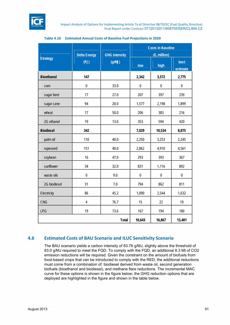
Impact Analysis of Options for Implementing Article 7a of Directive 98/70/EC (Fuel Quality Directive) Final Report under Contract 071201/2011/608705/SER/CLIMA.C2
August 2013 91
Table 4.10 Estimated Annual Costs of Baseline Fuel Projections in 2020
Strategy Delta Energy
(PJ)
GHG intensity
(g/MJ)
Costs in Baseline
(€, million)
low high best
estimate
Bioethanol 147 2,342 3,572 2,775
corn 0 33.0 0 0 0
sugar beet 17 27.0 207 397 239
sugar cane 94 20.0 1,577 2,198 1,899
wheat 17 50.0 206 383 216
2G ethanol 19 13.0 353 594 420
Biodiesel 342 7,029 10,534 8,875
palm oil 110 40.0 2,250 3,253 2,245
rapeseed 151 40.0 2,862 4,910 4,561
soybean 16 47.0 293 393 367
sunflower 34 32.0 831 1,116 892
waste oils 0 9.0 0 0 0
2G biodiesel 31 7.0 794 862 811
Electricity 86 45.2 1,090 2,544 1,632
CNG 4 76.7 15 22 19
LPG 19 73.6 167 194 180
Total 10,643 16,867 13,481
4.6 Estimated Costs of BAU Scenario and ILUC Sensitivity Scenario
The BAU scenario yields a carbon intensity of 83.76 g/MJ, slightly above the threshold of 83.0 g/MJ required to meet the FQD. To comply with the FQD, an additional 8.3 Mt of CO2 emission reductions will be required. Given the constraint on the amount of biofuels from food-based crops that can be introduced to comply with the RED, the additional reductions must come from a combination of: biodiesel derived from waste oil, second generation biofuels (bioethanol and biodiesel), and methane flare reductions. The incremental MAC curve for these options is shown in the figure below; the GHG reduction options that are deployed are highlighted in the figure and shown in the table below.

Impact Analysis of Options for Implementing Article 7a of Directive 98/70/EC (Fuel Quality Directive) Final Report under Contract 071201/2011/608705/SER/CLIMA.C2
August 2013 92
Table 4.11 Incremental Marginal Abatement Cost Curve for FQD Compliance in BAU Scenario
Table 4.12 Estimated Additional Cost of FQD Compliance for BAU in 2020
Strategy Increased
Energy (PJ)
GHG Reductions
(Mt)
Best Estimate (€, million)
Biodiesel, waste oil 20 1.6 -13
Methane flare reduction -- 6.7 7
Total 20 8.3 -6
The BAU scenario only has 31 PJ of biodiesel from waste oil consumed annually; this is consistent with current levels of consumption of biodiesel from recycled vegetable oils and animal fats (or tallow) according to the USDA Foreign Agriculture Service (FAS) in the EU. The EU FAS estimated consumption of 24.5 PJ of biodiesel from recycled vegetable oils and 14.7 PJ of biodiesel from animal fats in 2010.33. According to recent report,34 there is 83 PJ of potential for biodiesel from used cooking oil and another 10-48 PJ of potential for biodiesel from by-products in the food industry (e.g., animal fats). For the purposes of this report, we use a conservative estimate of 85 PJ. The estimated production costs of biodiesel from waste oil in 2020 are less than diesel; therefore, the small savings of €13 million (compared to total costs of €12.5 billion in the baseline) are realized by displacing diesel. These savings are offset slightly by just over €7 million required to achieve methane flare reductions of the remaining 6.7 Mt.
33 EU Biofuels Annual 2012. GAIN Report NL2020. Available online at: http://www.usda-france.fr/media/Biofuels%20Annual_The%20Hague_EU-27_6-25-2012.pdf 34 CE Delft, 2012. Sustainable Alternatives for land-based biofuels in the European Union: Assessment of options and development of a policy strategy. Available online at; http://www.cedelft.eu/publicatie/sustainable_alternatives_for_land-based_biofuels_in_the_european_union/1325
Biodiesel, Waste Oil
Biodiesel, Waste Oil
UER
‐50
0
50
100
150
200
0 10 20 30 40 50 60
MAC, Increm
ental Costs (€/t)
GHG Abatement (Mt)
Emission Reductions Requiredfor FQD Compliance in BAU

Impact Analysis of Options for Implementing Article 7a of Directive 98/70/EC (Fuel Quality Directive) Final Report under Contract 071201/2011/608705/SER/CLIMA.C2
August 2013 93
After accounting for ILUC values, as discussed in more detail in Section 3 (Task 1.2), the baseline fuel projections are further outside compliance with the FQD GHG emission targets. Based on direction from the European Commission, ICF displaced any biofuel that had a carbon intensity which did not achieve a 50% GHG reduction compared to fossil diesel or petrol: Bioethanol from wheat (no process fuel specified and natural gas used in a CHP plant) and biodiesel derived from palm oil, rapeseed, soy, and sunflower were removed from the fuel projections in 2020. The displaced demand was assumed to be replaced by fossil petrol and diesel. In order to comply with the FQD in this extreme scenario, as in the case of the baseline scenario, we assumed a combination of biofuels and upstream emission reductions in the oil and gas sector via methane flare reduction would be implemented to achieve compliance with the FQD – using the marginal abatement costs shown in Table 4.13. After displacing demand for bioethanol from wheat and biodiesel from palm oil, rapeseed, soybeans, and sunflower the total energy from renewables dropped to 2.5% of the transportation fuel mix.
Table 4.13 Incremental Marginal Abatement Cost Curve for FQD Compliance in ILUC Sensitivity Scenario
The increase in GHG emissions from increased demand for diesel required an additional 45.3 Mt CO2 reduction. Based on the MAC curve for strategies to comply with the FQD, additional bioethanol from corn, biodiesel from waste oils, and second generation biodiesel were taken up with methane flare reduction options. The methane flare reductions account for 34.5 Mt CO2 of the 54.3 Mt required for compliance at a cost of €914 million. The increased consumption of bioethanol from corn yields savings of €123 million; the additional biodiesel from waste oils and second generation feedstocks (non-land using) yield an additional cost of €373 million. The biggest cost contributor is the additional petroleum-derived diesel consumed by the displaced biodiesel from palm oil, soybean, rapeseed, and sunflower. The cost of the additional diesel consumption, at 575 PJ, is about €10.8 billion. This increase in costs is offset entirely by the displaced costs of the more expensive biodiesel from palm, soy, rapeseed, and sunflower.
Including accounting for the additional CO2 reduction strategies required to comply with the FQD because of ILUC emissions, we estimate savings of about €5.8 billion (as shown in the table below).
‐100
‐50
0
50
100
150
200
0 10 20 30 40 50
MAC, Incremental Costs (€/t)
GHG Abatement (Mt)
Emission Reductions Required for FQD Compliance in ILUC Sensitivity Scenario
Bioethanol, corn
Biodiesel, waste oil
Biodiesel, 2G non‐land
UER

Impact Analysis of Options for Implementing Article 7a of Directive 98/70/EC (Fuel Quality Directive) Final Report under Contract 071201/2011/608705/SER/CLIMA.C2
August 2013 94
Table 4.14 Estimated Annual Costs of ILUC Sensitivity Scenario in 2020
Step 1:
Account for ILUC Step 2:
FQD Compliance Total
Strategy Energy (PJ)
Best Estimate
(€, million)
Energy (PJ)
GHG reductions
(Mt)
Best Estimate
(€, million)
Energy (PJ)
Best Estimate
(€, million)
Bioethanol, wheat -30 -564 -- -- -30 -564
Biodiesel, palm -164 -3,928 -- -- -164 -3,928
Biodiesel, rapeseed -385 -10,033 -- -- -385 -10,033
Biodiesel, soy -105 -2,169 -- -- -105 -2,169
Biodiesel, sunflower -40 -1,040 -- -40 -1,040
Diesel, conventional 694 13,039 -119 -- -2,235 575 10,803
Petrol, conventional 30 521 -30 -521 0 0
Bioethanol, corn -- 30 1.3 -123 30 -123
Biodiesel, waste oil -- 54 4.3 20 54 20
Biodiesel, 2G non land using -- 65 5.2 353 65 353
Methane flare reduction -- -- 34.5 838 -- 838
Total 0 -4,174 0 45.3 -1,668 0 -5,843

Impact Analysis of Options for Implementing Article 7a of Directive 98/70/EC (Fuel Quality Directive) Final Report under Contract 071201/2011/608705/SER/CLIMA.C2
August 2013 95
5 Development of options (Task 2.1)
5.1 Introduction
This section sets out in the following manner:
■ Description of the alternative options for suppliers to determine their overall GHG intensities. These options are variously based on different levels of aggregation of default unit GHG intensities and options for developing actual unit GHG intensities that reflect crude/fuel pathways.
■ Description of supplier-specific options in more detail.
■ Presentation of a comparison and evaluation of the options against certain criteria and shortlisting of 3 options that will be analysed further under Task 2.2 following discussion and agreement with the Commission.
5.2 Description of options
5.2.1 Introduction
Key terms used to describe the options include:
■ Unit GHG intensities: these are default or actual GHG intensities that are specific to a certain fuel, or fuel and feedstock pathway where disaggregated, that a supplier will use to determine his total GHG intensity. The following options for unit GHG intensities exist:
■ Default average unit GHG intensities: These are the unit GHG intensities that are determined by the Commission, Member States, or a group of suppliers, used as standard values and derived from average or reference values (such as default values contained in the Commission proposal), which are specific for each fuel type, and in some cases are further disaggregated by feedstock.
■ Conservative default unit GHG intensities: in contrast to average default values, conservative default values are set higher than the weighted average values.
■ Actual unit GHG intensities: These are the unit GHG intensities that are determined by the supplier and are calculated using information that is specific to each fuel, feedstock and the operations of the supplier and all parties along its supply chain. This can be based on actual measured data or estimated. These are referenced in this text as ‘’supplier specific’’.
■ Total GHG intensity: this is the total GHG intensity for a supplier, that is calculated by the supplier, taking into account all the fuels (and their underlying feedstock pathways where disaggregated) supplied.
Note: throughout, the following notation is used:
I GHG intensity (units g CO2e / MJ) (“GHGi” in the Commission proposal)
Isupplier total GHG intensity
IEU or 3rd unit GHG intensity
f feedstock
p product (fuel) (“f” in the Commission proposal)
AF adjustment factors for powertrain efficiency (unit-less)
E energy supplied (units MJ) (“MJ” in the Commission proposal)
EU aggregate for EU-wide
Impact Analysis of Options for Implementing Article 7a of Directive 98/70/EC (Fuel Quality Directive) Final Report under Contract 071201/2011/608705/SER/CLIMA.C2
August 2013 96
MS aggregate at Member State level
3rd aggregate of 3rd country (countries outside of EU) imports
supplier aggregate at supplier level
UER upstream emission reduction in g CO2eq
The options that are presented and described are variously spaced on a scale of specificity and aggregation of data and factors. This ranges from option 0 which requires all suppliers to utilise EU-wide unit GHG intensities that are specified for each product (i.e. without specification of the feedstock), to option 5 which provides suppliers the option to develop their own supplier-specific unit GHG intensities reflecting their specific feedstock-product pathways that take into account the separate elements in the life cycle assessment. The less specific options require more aggregated data which is more straightforward to obtain, whilst the more supplier specific options carry greater data requirements. A summary table of the key characteristics of options 0 to 5 are shown in Table 5.135.
35 Note that the evaluations focus on options 1 to 5, and not 0 as this is the baseline rather than a potential policy option.

Impact Analysis of Options for Implementing Article 7a of Directive 98/70/EC (Fuel Quality Directive) Final Report under Contract 071201/2011/608705/SER/CLIMA.C2
August 2013 97
Table 5.1 Summary table of key characteristics of options (Note 1)
Option Method Type Party Determining unit GHG Intensity
Level of Disaggregation for unit GHG Intensity Unit GHG Intensity Specific to Feedstock
Mix of: By fuel type By feedstock
type Feedstock
categorisation By refinery
where produced
0 Default unit GHG intensity for the European Union
EC ✓ × N/A × EU
1 Default unit GHG intensity for the European Union by feedstock EC ✓ ✓
10 categories, specified in EC
proposal (Note 2) ✓ EU
2 Default unit GHG intensity for each Member State (MS)
EC / MSs ✓ × N/A × MS
3
Opt-In Default GHG intensity for opt-in suppliers by each feedstock type EC (Note 3) ✓ ✓
10 categories, specified in EC
proposal (Note 2) ✓
All suppliers choosing to Opt-In
Opt-Out
Actual GHG intensity for each supplier or supplier group by feedstock type
Supplier or group of suppliers ✓ ✓
Actual feedstocks per product per
supplier ✓
Supplier or group of suppliers choosing to Opt-
out
4
Opt-In Conservative default GHG intensity for the European Union by feedstock type EC ✓ ✓
10 categories, specified in EC
proposal (Note 2) ✓ EU
Opt-Out
Actual GHG intensity for each supplier or supplier group by feedstock type
Supplier or group of suppliers ✓ ✓
Actual feedstocks per product per
supplier ✓
Supplier or group of suppliers

Impact Analysis of Options for Implementing Article 7a of Directive 98/70/EC (Fuel Quality Directive) Final Report under Contract 071201/2011/608705/SER/CLIMA.C2
August 2013 98
Option Method Type Party Determining unit GHG Intensity
Level of Disaggregation for unit GHG Intensity Unit GHG Intensity Specific to Feedstock
Mix of: By fuel type By feedstock
type Feedstock
categorisation By refinery
where produced
5 Actual GHG intensity for each supplier Supplier or group of
suppliers ✓ ✓ Actual feedstocks per product per
supplier ✓
Supplier or group of suppliers
Notes
1. It is noted that under all options Art 7a(4) of the FQD requires MSs to ensure that there is the option for a group of suppliers to choose to meet the lifecycle GHG reduction obligations jointly. In such a case they shall be considered a single supplier.
2. Conventional crude, natural bitumen, oil shale, any fossil sources, coal converted to liquid fuel (with and without CCS), gas to liquids, natural gas (steam reforming), coal, coal with CCS, waste plastic.
3. On basis of supplier reporting from previous year(s)

Impact Analysis of Options for Implementing Article 7a of Directive 98/70/EC (Fuel Quality Directive) Final Report under Contract 071201/2011/608705/SER/CLIMA.C2
August 2013 99
The abatement choices that were screened for effectiveness to reduce life cycle greenhouse gas emissions intensities are set out in the table below.
Option Abatement choices for suppliers
Electric vehicles
Blending with
biofuels
Upstream emission
reductions
Switch feedstocks
(Note 1)
Reduce transportation GHG emission
intensities
Reduce refinery
GHG intensity*
Option 0
Option 1
Option 2
Option 3
Opt in
Opt out
Option 4
Opt in
Opt out
Option 5
Note
1. Supplier specific methods for these compliance options would have to address some key issues outlined below. Compliance options selected for modelling various avenues to compliance are specified in Section 6.2.4.
5.2.2 Key issues
■ Refineries produce multiple fuels from single or multiple feedstocks. This makes it difficult to deterministically link particular inputs with outputs, i.e. just because 20% of a refinery’s feedstock is e.g. non-conventional it does not necessarily mean as a consequence that 20% of the refinery’s diesel output is from non-conventional feedstocks. However, for the purposes of simplification, policy options appraised in this report assume that x% of a refinery feedstock should be attributed to x% of the product refined in the refinery.
■ For the supplier specific approaches determining emission intensities as disaggregated levels e.g. per product, would require allocating refinery emissions among the products produced by the refinery. This is a complex subject, with multiple options. An overview of literature on this subject is included in section 5.3.2.2.
■ Some imported feedstocks to refineries are actually semi-finished feedstocks (e.g. vacuum gasoil, VGO) that have been processed in refineries, but which are sometimes further refined before being sold as transport fuels. These so called ‘intermediates’ may need distinct reference in methodologies, but in essence should be considered as feedstocks not products.
■ Regarding upstream emission reductions, it is unclear how a supplier’s emission reductions will not be accounted for in the LCA of other suppliers. This topic is explored further in section 5.2.8.
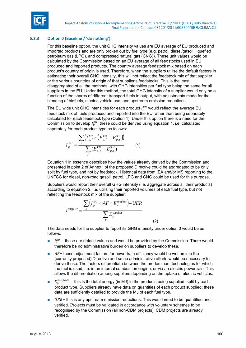
Impact Analysis of Options for Implementing Article 7a of Directive 98/70/EC (Fuel Quality Directive) Final Report under Contract 071201/2011/608705/SER/CLIMA.C2
August 2013 100
5.2.3 Option 0 (Baseline / ‘do nothing’)
For this baseline option, the unit GHG intensity values are EU average of EU produced and imported products and are only broken out by fuel type (e.g. petrol, diesel/gasoil, liquefied petroleum gas (LPG), and compressed natural gas (CNG)). These unit values would be calculated by the Commission based on an EU average of all feedstocks used in EU produced and imported products. The country average feedstock mix based on each product's country of origin is used. Therefore, when the suppliers utilise the default factors in estimating their overall GHG intensity, this will not reflect the feedstock mix of that supplier or the various countries of origin of that supplier’s feedstocks. This is the least disaggregated of all the methods, with GHG intensities per fuel type being the same for all suppliers in the EU. Under this method, the total GHG intensity of a supplier would only be a function of the shares of different transport fuels in output, with adjustments made for the blending of biofuels, electric vehicle use, and upstream emission reductions.
The EU wide unit GHG intensities for each product would reflect the average EU feedstock mix of fuels produced and imported into the EU rather than being separately calculated for each feedstock type (Option 1). Under this option there is a need for the Commission to develop ; these could be derived using equation 1, i.e. calculated separately for each product type as follows:
p
rdfp
EUfp
p
rdfp
EUfp
EUfp
EUp EE
EEI
I)( 3
,,
3,,,
(1)
Equation 1 in essence describes how the values already derived by the Commission and presented in point 2 of Annex I of the proposed Directive could be aggregated to be only split by fuel type, and not by feedstock. Historical data from IEA and/or MS reporting to the UNFCC for diesel, non-road gasoil, petrol, LPG and CNG could be used for this purpose.
Suppliers would report their overall GHG intensity (i.e. aggregate across all their products) according to equation 2, i.e. utilising their reported volumes of each fuel type, but not reflecting the feedstock mix of the supplier:
pp
pp
EUp
E
UEREAFI
I supplier
supplier
supplier
(2)
The data needs for the supplier to report its GHG intensity under option 0 would be as follows:
■ – these are default values and would be provided by the Commission. There would therefore be no administrative burden on suppliers to develop these.
■ − these adjustment factors for powertrain efficiency would be written into the (currently proposed) Directive and so no administrative efforts would be necessary to derive these. The factors differentiate between the predominant technologies for which the fuel is used, i.e. in an internal combustion engine, or via an electric powertrain. This allows the differentiation among suppliers depending on the uptake of electric vehicles.
■ – this is the total energy (in MJ) in the products being supplied, split by each product type. Suppliers already have data on quantities of each product supplied; these data are sufficiently detailed to provide the MJ of each fuel type.
■ − this is any upstream emission reductions. This would need to be quantified and verified. Projects must be validated in accordance with voluntary schemes to be recognised by the Commission (all non-CDM projects). CDM projects are already verified.

Impact Analysis of Options for Implementing Article 7a of Directive 98/70/EC (Fuel Quality Directive) Final Report under Contract 071201/2011/608705/SER/CLIMA.C2
August 2013 101
A worked example of Option 0 is presented in the box below:
Box 1 Worked example for Option 0
A supplier supplies the following fuels to the EU:
■ 1000 MJ of diesel imported from a US refinery. The US refinery is fed with feedstocks of conventional crudes and natural bitumen.
■ 2000 MJ of petrol from a UK refinery. The UK refinery is fed with feedstocks of conventional crudes.
The supplier does not mix biofuels nor invest in increasing uptake of electric vehicles, and has no certified upstream emission reductions.
Under Option 0 there is no need for suppliers to split their product energy according to feedstock type, hence the feedstock information for the refineries (and countries of origin) are redundant.
The default unit GHG intensities ( ) will be provided by the Commission and will only be split by product type, and will apply for all supplied fuels in the EU. For the purposes of this example, let us assume the following unit GHG intensities have been developed by the Commission: petrol 100 g CO2e/MJ, diesel or gas oil 102 g CO2e/MJ, LPG 73.6 g CO2e/MJ, CNG 76.7 g CO2e/MJ, hydrogen 90 g CO2e/MJ.
The supplier’s total GHG intensity is therefore (AF = 1 in all cases and is not shown):
pp
pp
EUp
E
UEREAFI
I supplier
supplier
supplier
MJeqCOg66.10020001000
020001001000102
2
5.2.4 Option 1 (Current proposal)
This option is the current Commission proposal for the implementing measure as proposed to the Fuel Quality Committee of Member State experts in October 2011.
The unit GHG intensity values in this option (denoted by , ) would be EU-wide default values per product and per feedstock type for conventional crudes (i.e. all conventional crudes together) and other feedstocks. These unit GHG intensity values have been derived by the Commission already and are, for option 1, the matrix of values in point 2 of Annex I of the Commission’s proposal.
The suppliers’ total GHG intensities would utilise the unit GHG intensities as per the Commission’s proposal from October 2011. Suppliers would estimate their own overall GHG intensity by multiplying each relevant unit GHG intensity by the energy associated with each feedstock / product combination. This option therefore requires the splitting of the supplier’s product energy (MJ) across feedstocks. This splitting is undertaken in Option 1 through the use of data on the refinery average feedstock mix per each product’s refinery of origin. Specifically, if the refinery is based on feedstocks comprising 90% conventional crudes and 10% natural bitumen (percentages are on an energy basis), then the products supplied will be split by this same percentage mix. Therefore, under option 1, the total GHG intensity of a supplier would be a function of the shares of different transport fuels in output together with the feedstock mix of the refinery(ies) of origin of the products, with adjustments made for the

Impact Analysis of Options for Implementing Article 7a of Directive 98/70/EC (Fuel Quality Directive) Final Report under Contract 071201/2011/608705/SER/CLIMA.C2
August 2013 102
blending of biofuels, electric vehicle use, and upstream emission reductions. The supplier’s total GHG intensity would be calculated according to equation 3:
pp
fpfp
EUfp
E
UEREAFI
I totalsupplier,
,
supplier,,
supplier (3)
This approach thus does rely on the actual feedstock mix at a refinery. The approach relies upon suppliers splitting their fuels (in terms of MJ) according to feedstock, i.e. ,
supplier.
Suppliers would split their fuels into each feedstock utilising the average feedstock mix of the refinery from which the product was sourced. Therefore this would require data on the average feedstock mix of each refinery of origin of the products. This obligation would exist equally for products refined in the EU as for products imported into the EU.
The splitting of the product energy using the percentage mix of feedstocks (on an energy basis) of a refinery makes the assumption that refineries’ use and choice of feedstocks is solely related to the products supplied that come within the scope of the FQD. Whilst the argument could be made that additional products are generated by refineries that are outside the scope of the FQD, and that consequently the feedstock mix specifically related to producing FQD fuels only could be considered to be different, for the purposes of simplicity, the total refinery feedstock mix (on an energy basis) is the mix assumed to apply to splitting the fuels by feedstock category.
In summary, the data needs for the supplier to report its GHG intensity under option 1, would be as follows:
■ , – these are the EU default values and would be provided by the Commission.
■ − these adjustment factors would be written into the (currently proposed) Directive.
■ , – this is the energy (in MJ) in the product being supplied, split by each product
type, and split by feedstock. Suppliers already have data on quantities of each product supplied; these data are sufficiently detailed to provide the MJ of each fuel type. Suppliers would also need to apportion the data on MJ of each fuel type across different feedstocks (at the level of granularity of the feedstock categories in the Commission’s proposal). This apportionment would be undertaken by utilisation of average mix of feedstocks for each refinery. These data would be utilised both for fuels produced in the EU as well as for fuels imported to the EU.
■ − this is the upstream emission reductions. This would need to be quantified and verified. Projects must be validated in accordance with voluntary schemes to be recognised by the Commission (all non-CDM projects).
The Commission's proposal also foresees that suppliers may make use of an actual calculation method for upstream emissions for fuel-feedstock combinations with GHG intensity higher than conventional crude. For reasons of simplicity this has not been addressed in the worked example below.
5.2.4.1 Producers (refiners)
A simple worked example of option 1 for suppliers that are producers of products is presented in the box below:
Box 2 Worked example for Option 1 – refiner supplier
A supplier supplies the following fuels to the EU:
■ 1000 MJ of diesel imported from a US refinery. The US refinery is fed with feedstocks of 80% conventional crudes and 20% natural bitumen.
■ 2000 MJ of petrol from a UK refinery. The UK refinery is fed with feedstocks of 100%

Impact Analysis of Options for Implementing Article 7a of Directive 98/70/EC (Fuel Quality Directive) Final Report under Contract 071201/2011/608705/SER/CLIMA.C2
August 2013 103
conventional crudes.
The supplier does not mix biofuels nor invest in increasing uptake of electric vehicles, and has no certified upstream emission reductions. A schematic of the supplier is shown below.
The diesel imported from the US would need to be split into the feedstock mix for the US refinery in question; the petrol from a UK refinery does not need to be split across feedstock categories as it is all from conventional crudes.
The supplier’s total GHG intensity is therefore (AF = 1 in all cases and is not shown):
pp
fpfp
EUfp
E
UEREAFI
I totalsupplier,
,
supplier,,
supplier
The above box outlined a simple description of the approach that a supplier with a refinery would estimate its total GHG intensity. Clearly, this is a simplified view and that depending on the type of supplier, different consequences would occur.
5.2.4.2 Traders
For suppliers that are only trading in products rather than refining them36, in order to split their product energy supplied by feedstock category according to the refinery (refineries) in which it was produced, these suppliers would have to ensure their products can be traced back to a refinery (or multiple refineries). Whilst the existing tracking system of fuel traded among Member States is the excise duty system, this system tracks quantities of taxable products passed through the duty system, not (meta-)information attached to each volume of product about the feedstock mix of the refinery from which it came. Therefore, for traders, there will be a requirement placed on them to determine the split of the product according to the feedstocks of the refineries in which it was produced. Where products supplied by traders have multiple origins (refineries) each of the pathways will need to be weighted by the energy (MJ) from each origin and each refinery’s feedstock mixes. The diagram below demonstrates this chain of custody in summary. This will require additional reporting and information pass-through that does not currently exist in the market.
36 For example, in Luxembourg, fuel suppliers are only traders since there are no refineries.
Supplier
US refinery
80% conventional crude
20% natural bitumen
UK refinery100%
conventional crude

Impact Analysis of Options for Implementing Article 7a of Directive 98/70/EC (Fuel Quality Directive) Final Report under Contract 071201/2011/608705/SER/CLIMA.C2
August 2013 104
5.2.4.3 Intermediates
CE Delft (2012)37 identified that ‘intermediate products’ form a significant part of the total petroleum product volumes. Intermediate products are refined products that undergo additional or further refining (reprocessing) within the EU in order to meet product standards (of sulphur content typically). Hence, despite the terminology of intermediate products, because these are required to be re-processed they actually form part of a feedstock for a refinery. As such, the use of feedstocks in refineries should be clarified that they should be included within a certain feedstock category. Two options exist here: to either classify intermediate products solely as one feedstock category (e.g. conventional crudes), or to determine the feedstock mix of the refinery of origin of the intermediates and to apply that mix as part of the overall calculation. If all intermediates were categorised in the ‘conventional crude’ feedstock category, this could potentially introduce a loophole for suppliers to use high carbon feedstocks to produce intermediates which are used as feedstocks classified as unconventional crudes. If intermediates were apportioned across feedstock categories in the ratio of the feedstocks for the refinery that produced the intermediates, i.e. as the alternative option, then the administrative burden would be increased (effectively, an extra level of supply chain).
The schematic below shows the hierarchy of how intermediates would be dealt with in the latter of these two options for treating intermediates.
37 CE Delft ‘Oil reporting for the FQD’ March 2012
Supplier
Refinery 1
Feedstock category A
Feedstock category B
Feedstock category C
Refinery 2Feedstock cateogry A
Refinery 3
Feedstock category B
Feedstock category C
Trader
%
%
%
%
%
%
%
%

Impact Analysis of Options for Implementing Article 7a of Directive 98/70/EC (Fuel Quality Directive) Final Report under Contract 071201/2011/608705/SER/CLIMA.C2
August 2013 105
5.2.5 Option 2
Option 2 incorporates the use of default values for unit GHG intensities, in a similar fashion to Option 0, but which are derived at Member State level. I.e. the unit GHG intensity values in this option would be Member State default values per fuel. ‘Member State default unit GHG intensities’ means the average, for each Member State, of GHG intensity of a fuel produced, based on the average feedstock mix of that Member State. The Member State default unit GHG intensities per fuel would also take into account of fuels (from 3rd countries or other Member States) calculated on basis of the average EU unit GHG intensity default values.
In order to calculate these values, the average feedstock mix for each Member State would be required to split into , , and similarly for imported fuels (intra EU and extra EU) the feedstock mix of the country of origin. It is anticipated that data are already available and collected on the average feedstock mix for each country. Historical data from IEA and/or MS reporting to the UNFCC for diesel, non-road gasoil, petrol, LPG and CNG could be used. Box 3 describes IEA data. The Member State default unit values could be derived by the Commission from the previously ascertained EU values , according to equation 4:
p
rdp
MSp
p
rdfp
EUimportsfp
MSfp
EUfp
MSp EE
EEEI
I)( 3
3,,,,
(4)
The results of this calculation for would be a matrix of values consisting of values per Member State for each product type, e.g. the average GHG intensity for petrol produced in that Member State.
Supplier
Refinery 1
Feedstock category A
Feedstock category B
intermediates Refinery
Feedstock category A
Feedstock category B
Refinery 2Feedstock cateogry A
Refinery 3
Feedstock category B
Feedstock category C
%
%
%
%
%
%
%
%
%
%

Impact Analysis of Options for Implementing Article 7a of Directive 98/70/EC (Fuel Quality Directive) Final Report under Contract 071201/2011/608705/SER/CLIMA.C2
August 2013 106
Box 3 IEA Crude Oil Import Register
The IEA collects monthly data on oil imports into IEA member countries disaggregated by major crude stream. The Crude Oil Import Register is a long standing reporting obligation for IEA member countries. The resulting data set is highly confidential. Data are collected on the following:
■ Number of importing companies ■ Volume [1000 bbl]
■ Sulphur content [%] ■ Value [in 1000 USD]
■ API gravity ■ Average costs [in USD/bbl]
The crude oil categories are defined by physical attributes (API, sulphur content) as well as country of origin, which are identified by region (8 regions), by country and as one of 105 crude streams.
A supplier’s total GHG intensity would multiply the Member State specific unit GHG intensities for each product with the energy of each product supplied. Under this method, the total GHG intensity of a supplier would be a function of the shares of different transport fuels in output, the feedstock mix of the Member State in which the product is supplied, with adjustments made for the blending of biofuels, electric vehicle use, and upstream emission reductions. Suppliers would use the following formula to calculate their overall GHG intensity:
pp
pp
MSp
E
UEREAFI
Isupplier
supplier
supplier (5)
As with options 0 and 1, this approach does not take into account actual unit GHG intensities of refined fuels or imported/traded fuels, as reflected in the schematic shown below.
Supplier
Member State origin of refined
product A
Total of feedstock category A
Total of feedstock category B
Total of feedstock category C
Member State origin of refined
product B
Total of feedstock category A
3rd country of origin of imported
product C
Total of feedstock category A
Total of feedstock category C
Supplier obligations EU/MS obligation

Impact Analysis of Options for Implementing Article 7a of Directive 98/70/EC (Fuel Quality Directive) Final Report under Contract 071201/2011/608705/SER/CLIMA.C2
August 2013 107
The data needs for equation 5, for the supplier to report its GHG intensity under option 2, would be as follows:
■ – these are unit default values and would be provided by the Commission. As identified above, these would rely on the average feedstock mix for each Member State, and for imported fuels, the feedstock mix of the country of origin. It is anticipated that data are already available and collected on the average feedstock mix for each country.
■ − these adjustment factors would be written into the (currently proposed) Directive.
■ – this is the energy (in MJ) in the product being supplied, split by each product type. Suppliers already have data on quantities of each product supplied; these data are sufficiently detailed to provide the MJ of each fuel type.
■ − this is the upstream emission reductions. This would need to be quantified and verified. Projects must be validated in accordance with voluntary schemes to be recognised by the Commission (all non-CDM projects).
The table below summarises the levels of disaggregation and averaging of the default unit GHG intensities among options 0, 1 and 2.
Option Disaggregation of unit GHG intensity :
Disaggregation Averaging
By product type
By feedstock category
At EU level At Member State level
At supplier level
Option 0
Option 1 (for products)
(for feedstock mix)
Option 2
A worked example of option 2 is presented in the box below:

Impact Analysis of Options for Implementing Article 7a of Directive 98/70/EC (Fuel Quality Directive) Final Report under Contract 071201/2011/608705/SER/CLIMA.C2
August 2013 108
Box 4 Worked example for Option 2
A UK supplier supplies the following fuels to the UK:
■ 1000 MJ of diesel imported from a US refinery. The US refinery is fed with feedstocks of conventional crudes and natural bitumen.
■ 2000 MJ of petrol from a UK refinery. The UK refinery is fed with feedstocks of conventional crudes.
The supplier does not mix biofuels nor invest in increasing uptake of electric vehicles, and has no certified upstream emission reductions.
Option 2 requires the Commission and Member States (i.e. not the supplier) to develop unit GHG intensities per product that are specific to each MS (i.e. reflect the feedstock mix of that Member State). Option 2 as currently described implies that imported and traded fuels are taken into account by the Commission and the Member States in the development of the MS specific unit GHG intensities rather than having separate factors applied by the supplier. For the purposes of this example, the value of for petrol
produced in the UK (i.e., petrolUK ) is assumed to be 90 g CO2e/MJ. For the diesel imported
from a US refinery, it is no longer relevant that the supplier has imported it from the US in this option, and it is instead only necessary to apply the values of that are relevant for the Member States in which the diesel (imported from the US) is supplied. Practically speaking, there would be a verification step at this point to verify that the fuel has been consumed in the UK. Since the supplier is based in the UK, the applicable unit GHG intensity is diesel
UK ., which is assumed to be 92 gCO2e/MJ for this example.
The supplier’s total GHG intensity is therefore (AF = 1 in all cases and is not shown):
pp
pp
MSp
E
UEREAFI
Isupplier
supplier
supplier
MJeqCOg66.9020001000
0100092200090
2

Impact Analysis of Options for Implementing Article 7a of Directive 98/70/EC (Fuel Quality Directive) Final Report under Contract 071201/2011/608705/SER/CLIMA.C2
August 2013 109
Box 5 Different intensities calculated under Option 1 and Option 2 For the purposes of an example comparison of options 1 and 2, we assume that a UK based supplier is supplying 1000MJ of diesel to the UK from a US refinery. Assuming that the US refinery in question has a feedstock mix of 80% conventional crude and 20% natural bitumen and that the applicable unit GHG intensity for option 2 in the UK is 92 gCO2e/MJ. It is also assumed that AF = 1, and UER = 0.
Option 1
pp
fpfp
EUfp
E
UEREAFI
I totalsupplier,
,
supplier,,
supplier
E , simplifies since the only product p is diesel
so only needs to be split into the portion of diesel
originating from each feedstock E , . This
apportionment is to be done on the basis of the feedstock mix of the refinery: in the example it is 80% conventional crude and 20% natural bitumen, i.e.
E , E ,
E ,
800MJ 200MJ
The relevant values of I , that are required in this
calculation are hence I , and
I , . These values are taken from
the EC implementing measure proposal of Oct 2011, i.e. 89.1gCO2e/MJ and 108.5gCO2e/MJ respectively.
The supplier’s GHG intensity is therefore:
MJegCO
I
/298.921000
1005.108(%)8010001.89(supplier
Option 2
pp
pp
MSp
E
UEREAFI
Isupplier
supplier
supplier
simplifies since in this example the only
product p is diesel. Hence the total
1000
The relevant value of that is required in this
calculation is . This value is assumed for the purposes of this example to be 92gCO2e/MJ.
The supplier’s GHG intensity is therefore:
MJegCOI /2921000
)100092(supplier
5.2.6 Suppliers meeting the reduction obligation jointly
Regarding the possibility of suppliers meeting the reduction obligation jointly, according to Article 7a(4) of the FQD, if this possibility was chosen by a group of suppliers, the group of suppliers would need to jointly report a total GHG intensity that would be calculated from a

Impact Analysis of Options for Implementing Article 7a of Directive 98/70/EC (Fuel Quality Directive) Final Report under Contract 071201/2011/608705/SER/CLIMA.C2
August 2013 110
weighted average of the intensities of each member of the group, which in turn would be calculated as previous described. The weighting would continue to be on the energy basis (MJ supplied). Suppliers would not need to establish alternative unit GHG intensities; each supplier in the group would need to establish volumes (MJ) of product supplied split with the appropriate granularity for the methodology (i.e. with or without feedstock disaggregation depending on the methodology). There could potentially be the need for multiple Member State competent authorities to be involved e.g. in verification processes with associated verification costs.
As long as any methodology option does not require groups of suppliers to meet the reduction obligation jointly, then there is not expected to be a legal hurdle in relation to Article 7a(4) of the FQD. If however any option was implemented with a requirement that all suppliers in the EU or a Member State must meet the reduction obligation jointly then this would seem to contradict Article 7a(4) which gives suppliers the option of joining together for compliance purposes.
5.2.7 Option 3
Option 3 is a hybrid option that provides suppliers with a choice to either "opt-in" and use average default unit GHG intensities values (similarly to those applied in option 1) or to "opt-out" and develop actual values for GHG intensities at the same level of disaggregation as Option 1 (i.e. per fuel and per feedstock type). For a subsequent year of reporting, the default unit GHG intensity values that would apply for those suppliers that opt in would be adjusted to take account of those suppliers that opted out of this approach in the original year of reporting.
In the first year of implementation, if all suppliers opt in, then Option 3 is functionally the same as Option 1. It all suppliers opt-out, Option 3 is essentially Option 5.
Suppliers’ choices about whether to opt in or opt out are expected to be based on which provides the supplier with a lower total GHG intensity because this would reduce compliance costs. Those suppliers with actual unit GHG intensities lower than the initial EU default unit GHG intensities would be expected to opt out as they would stand to benefit from this by way of reduced total GHG intensities and hence reduced distances to targets. If
Group of suppliers
Supplier 1
Refinery AFeedstock category A
Refinery BFeedstock category D
Refinery C
Feedstock category B
Feedstock category C
Supplier 2 Refinery DFeedstock category A
Supplier 3
Refinery E
Feedstock category A
Feedstock category C
Refinery FFeedstock category A
%
%
%
%
%
% %
%
%
%
%
%

Impact Analysis of Options for Implementing Article 7a of Directive 98/70/EC (Fuel Quality Directive) Final Report under Contract 071201/2011/608705/SER/CLIMA.C2
August 2013 111
the default unit GHG intensity is recalculated (upwards) for a subsequent year, then additional suppliers would be expected to opt out. Therefore the proportion of suppliers that opt out will increase with each recalculation; the proportion that opts out each iteration depends on (1) the distribution of GHG intensities and (2) the costs of opting out. An overview of the option across each iteration is shown in the table below.
5.2.7.1 Opt‐in suppliers
For those suppliers that choose to opt in, in the first year of implementation the average default unit GHG intensities values would be those in Option 1, i.e. EU-wide default values per fuel and per feedstock type (with the break-out of feedstock categories as per the Commission’s proposal, i.e. all conventional crudes together, and certain other named feedstocks). These have been derived by the Commission already and are the matrix of values in point 2 of Annex I of the Commission’s proposal.
Under this method, the total GHG intensity of a supplier would be a function of the shares of different transport fuels in output split according to the feedstock mix of the refinery of origin of products, with adjustments made for the blending of biofuels, electric vehicle use, and upstream emission reductions.
However, in order to ensure that the default values that would apply to the opted in suppliers would best reflect the opted-in suppliers’ actual intensities, option 3 would use these existing default values as a starting point only for the first year of implementation. For the second iteration in implementation of reporting38, there would be a need to adjust these default values to reflect the portion of the market that chose to opt-out in the first year. This adjustment would need to take into account the volume of fuel placed on the market by suppliers choosing to opt out in the first year, as well as the GHG intensities reported by these opting out suppliers in the first year. As indicated above, suppliers with expected actual unit intensities higher than the default values would be the group of suppliers that would stand to benefit from opting in under Option 3, as these suppliers would minimise their reported emissions. Clearly, for these opted in suppliers, their reported emissions would likely be lower than their actual emissions. This is the driver for the adjustment to the default values: to reduce the disparity between the reported emissions and the actual emissions. Hence, the default unit GHG intensities would be adjusted by the Commission to better represent the proportion of the suppliers opting in.
The suppliers expected to opt out are those with unit GHG intensities lower than the default unit GHG intensities. The default unit GHG intensities reflect (for the first year of implementation) the entire market of suppliers of known volumes supplied. Hence, the adjustment to the default unit GHG intensities by removing the portion attributable to the
38 Frequency of the iteration would be confirmed by the Commission. Annually is a minimum; every three years may be more realistic in order to receive, verify and analyse data from opted out suppliers, and to then re-calculate the unit GHG intensity values.
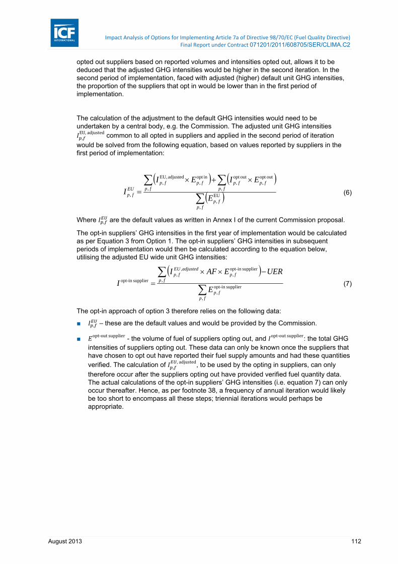
Impact Analysis of Options for Implementing Article 7a of Directive 98/70/EC (Fuel Quality Directive) Final Report under Contract 071201/2011/608705/SER/CLIMA.C2
August 2013 112
opted out suppliers based on reported volumes and intensities opted out, allows it to be deduced that the adjusted GHG intensities would be higher in the second iteration. In the second period of implementation, faced with adjusted (higher) default unit GHG intensities, the proportion of the suppliers that opt in would be lower than in the first period of implementation.
The calculation of the adjustment to the default GHG intensities would need to be undertaken by a central body, e.g. the Commission. The adjusted unit GHG intensities
,EU,adjusted common to all opted in suppliers and applied in the second period of iteration
would be solved from the following equation, based on values reported by suppliers in the first period of implementation:
fpfp
fpfpfp
fpfpfp
EUfp E
EIEI
I
,
EU,
,
outopt ,
outopt ,
,
inopt ,
adjusted EU,,
, (6)
Where , are the default values as written in Annex I of the current Commission proposal.
The opt-in suppliers’ GHG intensities in the first year of implementation would be calculated as per Equation 3 from Option 1. The opt-in suppliers’ GHG intensities in subsequent periods of implementation would then be calculated according to the equation below, utilising the adjusted EU wide unit GHG intensities:
fpfp
fpfp
adjustedEUfp
E
UEREAFI
I
,
supplierin -opt,
,
supplierin -opt,
,,
supplierin -opt (7)
The opt-in approach of option 3 therefore relies on the following data:
■ , – these are the default values and would be provided by the Commission.
■ opt‐outsupplier - the volume of fuel of suppliers opting out, and opt‐outsupplier: the total GHG intensities of suppliers opting out. These data can only be known once the suppliers that have chosen to opt out have reported their fuel supply amounts and had these quantities verified. The calculation of ,
,adjusted, to be used by the opting in suppliers, can only
therefore occur after the suppliers opting out have provided verified fuel quantity data. The actual calculations of the opt-in suppliers’ GHG intensities (i.e. equation 7) can only occur thereafter. Hence, as per footnote 38, a frequency of annual iteration would likely be too short to encompass all these steps; triennial iterations would perhaps be appropriate.

Impact Analysis of Options for Implementing Article 7a of Directive 98/70/EC (Fuel Quality Directive) Final Report under Contract 071201/2011/608705/SER/CLIMA.C2
August 2013 113
Box 6 Worked example for Option 3 – opted in suppliers
Option 3 is functionally the same as Option 1 for opted in suppliers in terms of the level of disaggregation of fuel and feedstocks that are necessary. The only difference is that the unit GHG intensities applied by the suppliers would be adjusted from those default unit GHG intensities applied under Option 1. But since the adjustment is undertaken by the Commission rather than by the suppliers, the supplier follows the same methodology, i.e. for a supplier supplying the following fuels to the EU, and which does not mix biofuels nor invest in increasing uptake of electric vehicles, and who has no certified upstream emission reductions:
1000 MJ of diesel imported from a US refinery. The US refinery is fed with feedstocks of 80% conventional crudes and 20% natural bitumen. [in practice the feedstock mix would need to be specified to the same number of feedstock categories as in the Commission’s proposal]
2000 MJ of petrol from a UK refinery. The UK refinery is fed with feedstocks of 100% conventional crudes.
The supplier’s total GHG intensity would be (assuming the same unit GHG intensities, i.e. year 1 of implementation, and that AF = 1 in all cases and is not shown):
pp
cfpcfp
EUfp
E
UEREAFI
I totalsupplier,
,,
supplier,,,
supplier
MJeqCOg3.8920001000
20005.872.010005.1088.010001.89
2
5.2.7.2 Opt‐out suppliers
This option assumes (and has been modelled on the basis) that the opportunity to opt out is a choice available for a supplier as a whole. It is not an option for suppliers to choose which of their feedstock-fuel pathways to opt-in or opt-out. However it is noted that the provision of the possibility to opt in or opt out individual feedstock-fuel pathways could potentially provide useful flexibility for suppliers to utilise data that is available for part of their fuels but being able to rely on the default value approach for those pathways in their supply chain for which they do not have access to relevant data.
Suppliers choosing to opt out of using the EU-wide default unit GHG intensities would develop their own estimate for total GHG intensity based on their actual feedstock-fuel pathways, i.e. based on a life cycle assessment (LCA) estimate that is consistent in scope to the default unit GHG intensities. For example, suppliers could develop their own supplier-specific (i.e. actual) unit GHG intensities for each fuel and feedstock combination,
,opt‐outsupplier, rather than use default values e.g. , . Suppliers’ total GHG intensity would
then be calculated as follows:
fpfp
fpfpfp
E
UEREAFI
I
,
supplierout -opt,
,
supplierout -opt,
supplierout opt,
supplierout -opt (8)

Impact Analysis of Options for Implementing Article 7a of Directive 98/70/EC (Fuel Quality Directive) Final Report under Contract 071201/2011/608705/SER/CLIMA.C2
August 2013 114
Alternatively, each pathway could be assessed on an LCA basis, and the volume of product produced under each pathway used to develop a weighted average total GHG intensity. For opted out suppliers, their total GHG intensity would be expected to be a function of the following elements:
■ the supplier’s feedstocks, which will be derived from refinery feedstock data at the refinery level (see Section 5.3.4.3 on availability of feedstock data for individual refineries)
■ the shares of different transport fuels in output,
■ the emissions intensity of the feedstock and product transportation,
■ the emissions intensity of the refining operations of the supplier,
■ and with adjustments made for the blending of biofuels, electric vehicle use, and upstream emission reduction projects.
Details on the feasibility of developing and employing supplier-specific unit GHG intensities are described in section 5.3. Compliance options taken up in the subsequent evaluation are described in Section 6.2.4.
As with other options in which suppliers can develop their own LCA, this raises the issue concerning any upstream emission reduction (UER) projects that suppliers are able to take account of in their reporting under opt in options presented thus far (e.g. equations 2, 3, 5 and 7) should not be double counted by suppliers that utilise feedstocks from the same upstream extraction process in which an emission reduction project has been implemented, certified, verified and claimed by a supplier. This is elaborated further below.
5.2.8 Upstream Emission Reductions
The consequence of needing to avoid double counting of claimed or registered upstream emission reduction (UER) projects in methodologies that rely on LCAs of actual emission pathways is that the EU would need to at least facilitate a platform for cross-checking listed projects against claimed LCAs.
The EC or a designated executive agency would need to administer a centrally coordinated database of UER projects. This would lead to costs to the EC to develop and maintain the database, as well as costs for suppliers to access the database to ensure no double counting.
Although such a database would be required under all the options that provide suppliers the possibility to use UER ‘credits’, the administration and implementation would be more straightforward for methodologies that do not rely on suppliers’ own LCAs. This is because for methodology options 0, 1 and 2, UERs would only be available to each supplier that has that UER registered in their name. Hence verification that UERs are applied correctly would simply rely on the robustness of awarding UERs, and cross-checking that any UER claimed by a supplier is indeed registered to that supplier.
However, it is more complex for methodology options that provide suppliers with the opportunity to develop their own estimates of emission intensity, but which retain the possibility for suppliers to utilise UER credits. Suppliers that develop own estimates of pathway lifecycle emissions that happen to use a same crude origin for which a UER project from another supplier is already implemented will need to be aware of this existing UER project, and it could be required of the supplier to calculate their emissions as if the UER didn’t exist (i.e. to avoid double counting). For example, if a flare reduction project funded by supplier A reduces flaring at extraction site X by 80%, and then supplier B subsequently sources crude from that same extraction site X then supplier B will benefit from the reduced emissions of the extraction phase but only if they develop their own LCA estimates, e.g. option 3 opt out. Supplier B would then essentially be double counting the UER if their LCA took account of the 80% reduced flaring at the extraction site X. However, to avoid this double counting, for example through requiring supplier B to estimate LCA emissions as if the flaring hadn’t been reduced, would disincentivise supplier B (or other suppliers) from

Impact Analysis of Options for Implementing Article 7a of Directive 98/70/EC (Fuel Quality Directive) Final Report under Contract 071201/2011/608705/SER/CLIMA.C2
August 2013 115
getting crude from extraction site X and would discourage them from developing their own emissions. If the double counting was allowed, then this may reduce the market demand for original UER projects since free-ridership could occur. This results in a complex market interaction.
5.2.9 Option 4
Similarly to Option 3, Option 4 is a hybrid option that provides suppliers with a choice to either "opt-in" and use conservative default unit GHG intensities values at the same level of disaggregation as Option 1 (i.e. per fuel and per feedstock type) or to "opt-out" and develop actual values for GHG intensities.
Through the use of conservative default values, which are set higher than the average default values, this option seeks to provide an incentive for suppliers to reduce the GHG intensity of fuels over time, manifest in this instance by an incentive for suppliers to determine their actual unit GHG intensities. The conservative default unit GHG intensities would be between the average and the upper bound of the range of possible GHG intensities for fuel products39, and therefore may be characteristic of more complex refineries and / or those that have higher feedstock GHG intensities. As in Option 1, unit GHG intensities will be determined separately for conventional crude and high-carbon feedstocks.
The advantages of conservative values are:
■ It would be consistent with the methodology already in place for biofuels
■ They would incentivise suppliers to make efforts to reduce their fuels’ life cycle GHG intensities
■ They would not have to be updated as often as the adjustment of the opt-in default unit GHG intensities of Option 3.
The disadvantages of conservative values are:
■ If the development of actual unit GHG intensities is too costly for suppliers, then the supplier defaults to using a conservative value which will tend to overestimate emissions.
■ By definition, the values overestimate actual emissions for more than half of suppliers’ fuel. This would run the risk of causing the reporting of such values not usable for the updating of the fossil fuel comparator.
If all suppliers opt-out, Option 4 converges to essentially be the same as Option 5. Suppliers’ choices about whether to opt in or opt out will be based on which gives lower total GHG intensity, as per option 3. It is only expected that those suppliers that anticipate having actual unit GHG intensities on average lower than the adjusted default values would choose to opt out. I.e. this opt-out option provides these suppliers the possibility to prove that their fuels have lower GHG intensities than other suppliers. The threshold for suppliers’ choices is essentially raised compared to option 3, so more suppliers are incentivised to develop actual data. Since opting out incurs a transaction cost (developing actual data), the decision boundary will be lower than the conservative defaults.
It should be noted that as low GHG intensive suppliers are more likely to choose to determine their actual GHG intensities, the extent to which the default intensity will remain conservatively high for the remainder of suppliers will diminish – i.e. once low GHG-intensive suppliers are opted out, what were ‘conservatively high’ values may not necessarily remain that high for the suppliers that remain opted in.
39 As identified in e.g. Brandt, A. (2011) Upstream greenhouse gas (GHG) emissions from Canadian oil sands as a feedstock for European refineries

Impact Analysis of Options for Implementing Article 7a of Directive 98/70/EC (Fuel Quality Directive) Final Report under Contract 071201/2011/608705/SER/CLIMA.C2
August 2013 116
5.2.9.1 Opt‐in suppliers
For the purposes of opt-in suppliers, the Commission would need to develop conservative values of , which are set at suitable levels to provide the intended level of incentive. In
order for the Commission to develop ,,conservative, decisions would need to be made as to
how far between the average values , (which may be based on ‘most likely values’ from Brandt, 2011) and the maximum values, e.g. identified in Brandt (2011), the conservative values ,
,conservative should be set. The figure below from Brandt (2011) demonstrates the
range within which the GHG intensities can be set.
Figure 5.1 Weighted‐average most likely oil sands emissions compared to weighted average conventional EU refinery feedstock. Source: Brandt (2011)
In order to understand the level of conservatism to set the unit GHG intensities, it will be important to have an understanding of the distribution of suppliers’ actual GHG intensities. Brandt (2011) estimated that the distribution of life cycle GHG emissions intensity of conventional crude imports to the EU consists of around 95% by volume in a narrow band of intensities, with the remaining 5% at appreciably increased intensities, as shown below in Figure 5.2.
Figure 5.2 Emissions as a function of cumulative normalized output, for oil sands projects and conventional oil imports to the EU. Source: Brandt (2011)
By way of comparison with Figure 5.3, the LCA carbon intensities included in the 2012 Jacobs study for the Alberta Government for specific crudes have been mapped where possible to the crudes identified as used in the EU in the baseline analysis of this study. Two

Impact Analysis of Options for Implementing Article 7a of Directive 98/70/EC (Fuel Quality Directive) Final Report under Contract 071201/2011/608705/SER/CLIMA.C2
August 2013 117
thirds of the crudes (by volume) were mapped in this way, and these have been shown below in Figure 5.3. Although in this figure the ‘hockey stick’ distribution is not observed, since around one third of the crude has not been mapped to carbon intensities a comparison with Figure 5.2 is not definitive.
Figure 5.3 GHG emissions intensity as a function of cumulative normalised EU crude use for crudes identified in the WORLD model for the baseline of Task 1 mapped to GHG intensity values from Jacobs (2012). Source: this work
The opt-in suppliers’ GHG intensities would be calculated according to the equation below, utilising the conservative EU wide unit GHG intensities:
fpfp
fpfp
EUfp
E
UEREAFI
I
,
supplierin -opt,
,
supplierin -opt,
veconservati ,,
supplierin -opt (9)
Under this method, the total GHG intensity of a supplier would be a function of the shares of different transport fuels in output split according to the feedstock mix of the refinery of origin of products, with adjustments made for the blending of biofuels, electric vehicle use, and upstream emission reductions.
5.2.9.2 Opt‐out suppliers
Suppliers determining actual GHG intensities are faced with the same procedures as in Option 3 (opt out) and Option 5. Equation 8 in section 5.2.7.2 remains valid for these suppliers. See option 5 and Section 3 for more information.
Under this method, the total GHG intensity of a supplier would be a function of the following elements:
■ the supplier’s feedstocks, which will be derived from refinery feedstock data at the refinery level (see Section 5.3.4.3 on availability of feedstock data for individual refineries),
■ the shares of different transport fuels in output,
■ the emissions intensity of the feedstock and product transportation,
■ the emissions intensity of the refining operations of the supplier,
■ and with adjustments made for the blending of biofuels, electric vehicle use, and upstream emission reduction projects.
Impact Analysis of Options for Implementing Article 7a of Directive 98/70/EC (Fuel Quality Directive) Final Report under Contract 071201/2011/608705/SER/CLIMA.C2
August 2013 118
Details on the feasibility of developing and employing supplier-specific unit GHG intensities are described in section 5.3. Compliance options taken up in the subsequent evaluation are described in Section 6.2.4.
Since options 3 and 4 both provide the possibility for suppliers to develop and use supplier-specific unit GHG intensities, for the portions of the market that choose this ‘opt-out’ route the accuracy of the GHG intensities that suppliers would report should be greater than the accuracies of options 0, 1 and 2. Due to the adjustment mechanism under the opt-in portion of option 3, the accuracy of opted-in suppliers’ GHG intensities should be greater than the intensities for those same suppliers reporting under option 1 (assuming that at least some suppliers do opt-out, as if not the result and accuracy of option 3 is the same as option 1).
The accuracy of the GHG intensities of suppliers opting in under option 4 is similarly (to option 3) to some extent dependent on the proportion of the market opting out: since the unit GHG intensities under option 4 are set conservatively high, the accuracy of this option if no suppliers opt out is lower than the accuracy of option 1 since emission intensities would overall be overestimated. But if a greater proportion of the market opts out then the conservatively high unit GHG intensities would begin to better reflect the actual intensities of the suppliers (assuming that the suppliers that do opt out are those with lower actual unit GHG intensities).
5.2.10 Option 5
With Option 5, suppliers must determine their own unit GHG intensities for each fuel product and feedstock type using an accepted standardized method. An example of such a method is ISO 14064, which sets minimum requirements for governments, businesses, and other organizations to quantify and report greenhouse gas emissions.40 GHG data would be collected from all parties along the supply chain including the producers, upstream processors, transporters, and refiners. Alternatively, approved estimation methods may be applied. These methods usually involve a third-party verification process where an external party must attest to the methods and calculations employed by the supplier to calculate their GHG intensity.
Under this method, the total GHG intensity of a supplier would be a function of the following elements:
■ the supplier’s feedstocks, which will be derived from refinery feedstock data at the refinery level (see Section 5.3.4.3 on availability of feedstock data for individual refineries),
■ the shares of different transport fuels in output,
■ the emissions intensity of the feedstock and product transportation,
■ the emissions intensity of the refining operations of the supplier,
■ and with adjustments made for the blending of biofuels, electric vehicle use, and upstream emission reductions.
Section 5.3 sets out further details on supplier-specific approaches. Compliance options taken up in the subsequent evaluation are described in Section 6.2.4.
40 International Organization for Standardization. “ISO 14064: International Standard for GHG Emissions Inventories and Verification”. Geneva, Switzerland.

Impact Analysis of Options for Implementing Article 7a of Directive 98/70/EC (Fuel Quality Directive) Final Report under Contract 071201/2011/608705/SER/CLIMA.C2
August 2013 119
5.2.11 Summary of equations
The table below compares the equations presented in the sections above.
Table 5.2 Summary of equations for deriving unit and total GHG intensities for each option
Equation to derive unit GHG intensities from option 1
Equation for supplier’s total GHG intensity
Op
tio
n 0
p
rdfp
EUfp
p
rdfp
EUfp
EUfp
EUp EE
EEI
I)( 3
,,
3,,,
pp
pp
EUp
E
UEREAFI
I supplier
supplier
supplier
Op
tio
n 1
N/A ( , set out in EC proposal)
pp
cfpcfp
EUfp
E
UEREAFI
I totalsupplier,
,,
supplier,,,
supplier
Op
tio
n 2
p
rdfp
MSfp
p
rdfp
MSfp
EUfp
MSp EE
EEI
I)( 3
,,
3,,,
pp
pp
MSp
E
UEREAFI
Isupplier
supplier
supplier
3 o
pt
in
fpfp
fpfpfp
fpfpfp
EUfp E
EIEI
I
,
EU,
,
outopt ,
outopt ,
,
inopt ,
adjusted EU,,
,
fpfp
fpfp
adjustedEUfp
E
UEREAFI
I
,
supplierin -opt,
,
supplierin -opt,
,,
supplierin -opt
3 o
pt
ou
t N/A supplier specific
fpfp
fpfpfp
E
UEREAFI
I
,
supplierout -opt,
,
supplierout -opt,
supplierout opt,
supplierout -opt
4 o
pt
in Conservative values, i.e. ( ,
EU,conservative) would
need to be developed
fpfp
fpfp
EUfp
E
UEREAFI
I
,
supplierin -opt,
,
supplierin -opt,
veconservati ,,
supplierin -opt
4 o
pt
ou
t N/A supplier specific As per option 3 opt out
Op
tio
n 5
N/A supplier specific Actuals, i.e. as per option 3 opt out

Impact Analysis of Options for Implementing Article 7a of Directive 98/70/EC (Fuel Quality Directive) Final Report under Contract 071201/2011/608705/SER/CLIMA.C2
August 2013 120
5.3 Supplier‐specific unit GHG intensities: Life Cycle Analysis (LCA)
5.3.1 Introduction
Option 5 as described above presents a policy option that requires suppliers to determine unit GHG intensities that are specific to the aggregate pathway of the fuel the supplier is supplying. This implies that the supplier-specific GHG intensity is based on actual data from the various stages of extraction through use of the final product. However, as described later in this section, there are practical limitations on developing actual data from specific geographic regions, as well as various options that could be utilised as fall-back approaches for when such limitations are reached (or which could be opted for voluntarily).
Life cycle analyses when undertaken for companies (e.g. following ISO 14044) are usually calculated for a typical pathway, rather than being calculated for each and every possible combination of LCA stages. When considering one crude, there may be multiple combinations of LCA stages that could be calculated. For example Nigerian crude may be processed in several different refineries each with different refining stage GHG intensity. Product delivery to retail stations can be different paths too.
For consideration of Task 2.2, the number of “actual” LCA pathways could be determined by analysing all the possible combinations of LCA stages for each crude production, transport, refining, and product delivery. Then total the costs from previous paragraphs, to determine total range of costs to implement “actual” LCA option.
For each of the life cycle stages, assessment is made (in section 3.4) of the options feasibility under the headings of:
■ Methods for data gathering – This summarises the methods potentially available to suppliers to develop emissions data. This includes considerations of methods not yet fully operable but for which additional work would be necessary to make the methods operable.
■ Source of data and availability – this identifies whether suppliers would feasibly be able to obtain data according to the methods described. For the use of LCA models, the key questions here concern whether the models sufficiently cover EU production and exporting regions in terms of feedstock used and refining configurations.
■ Verifiability – concerns the feasibility of suppliers obtaining verification of their data. Adequate verification would be according to the demands of the Member States.
■ Accuracy concerns how closely the method is likely to represent the actual GHG intensities of the suppliers and therefore that the error and uncertainty are at sufficiently low levels to achieve this. However, it is difficult to quantify the error / uncertainty. The Jacobs report includes a section on data uncertainty which indicates that “Lack of public information on energy consumption, gas venting, and flaring in crude oil production in the rest of world outside of Alberta forced us to estimate energy and GHG emissions using our models. These estimates of the carbon intensity of crude oils from the rest of the world could not be verified against field data.”
■ Implementation concerns the potential timescales in which the option could be operable.
5.3.2 LCA Methods and costs
5.3.2.1 Actual measured data
The ISO standard 14064 for developing GHG emission inventories41 includes scope for developing actual measured data. This part of the ISO standard details principles and requirements for verifying GHG inventories and validating or verifying GHG projects. It
41 International Organization for Standardization. “ISO 14064: International Standard for GHG Emissions Inventories and Verification”. Geneva, Switzerland.
Impact Analysis of Options for Implementing Article 7a of Directive 98/70/EC (Fuel Quality Directive) Final Report under Contract 071201/2011/608705/SER/CLIMA.C2
August 2013 121
describes the process for GHG-related validation or verification42 and specifies components such as validation or verification planning, assessment procedures and the evaluation of organisation or project GHG assertions43. The principles include relevance, completeness, consistency, accuracy, transparency, conservativeness and also includes an assessment of data management systems and controls. The ISO standard can be used by organisations or independent parties to validate or verify GHG assertions.
The Canadian Government (both Alberta and British Columbia) do currently require measured, operational and verified data for GHG reporting from crude oil extraction and refining. This requirement implies that it is possible to develop actual measured data for these activities.
The cost of measuring actual data for a company at one facility is estimated to be $30,000 to $50,000. Validation cost for one facility is about $15,000 to $25,000.44 The costs for a complete LCA for one supplier may draw on data from multiple facilities in the supply chain (e.g. multiple extraction facilities, and one or more refineries).
5.3.2.2 Estimation approaches
There are principally two ways of estimating GHG intensities within LCAs without drawing on actual measured data. The first is to develop ‘engineering estimates’ that can be used in LCA models, and the second is to utilise default values in existing LCA models.
Engineering estimates could be sought by suppliers from independent bodies (e.g. engineering consultants) who could either be engaged by suppliers to estimate GHG emissions/intensities from a single life cycle stage or to estimate GHG emissions/intensities from entire life cycles across all the permutations that one supplier may have (e.g. multiple feedstocks via multiple transport modes to multiple refineries, and multiple products being delivered to multiple locations.
The cost of an engineering estimate for one crude LCA is likely to be in the range of $90,000 to $120,000.45 A potential behavioural response by upstream suppliers is to undertake engineering estimates unilaterally in order to demand higher prices for the feedstocks in the EU. However it would be difficult for product supplier (refiner) to benefit from this as they would typically use many feedstocks (crudes) in a single month.
Engineering estimates are more accurate for crude oil production, upgrading and refining stages than relying on the default values incorporated in LCA models. Engineering estimates can be primarily undertaken for the crude extraction and refining stages of the life cycle. Validated engineering estimates are more accurate, but (as described below) engineering estimates can only typically be validated against measured, operational data for a LCA stage within the EU or North America. Engineering estimates are first principles estimates; this can include the use of refinery models; or upstream production models. These types of estimates or models are used by industry to assess/plan their own operations and have been utilised for a long time; they weren’t originally created for GHG analysis. In contrast for upstream production and refining, the LCA models, which have been developed in order to estimate GHG emissions, may involve simpler calculation methods and not be as accurate.
There are a number of LCA models that are available. These models have however a wide range of accuracy and, since there is no internationally agreed or accepted method for modelling LCA, vary in their methodologies. The following LCA models are considered as options for the estimates:
42 Validation is a process regarding future GHG performance. Verification is a process regarding past GHG performance. 43 A GHG assertion is an objective statement of performance related to GHGs made by a supplier, which could relate to GHG emissions, GHG emission reductions, or conformance to a GHG standard. 44 ICF expert estimate. 45 ICF expert estimate.
Impact Analysis of Options for Implementing Article 7a of Directive 98/70/EC (Fuel Quality Directive) Final Report under Contract 071201/2011/608705/SER/CLIMA.C2
August 2013 122
■ GREET (The Greenhouse Gases, Regulated Emissions, and Energy Use in Transportation Model)46. GREET allows researchers and analysts to evaluate various vehicle and fuel combinations on a full fuel-cycle/vehicle-cycle basis. The most recent fuel cycle analysis module is GREET 1 2012 rev2. It is a multidimensional spreadsheet model in Microsoft Excel, available for free in the public domain. For a given vehicle and fuel system, GREET estimates GHG emissions (CO2, CH4 and N2O) as well as energy consumption and various air pollutants. The model includes more than 100 fuel pathways including conventional and oil sands for petroleum fuels. The crudes in GREET are based on data from the EIA Annual Energy Outlook, and, based on this mix of crudes, there is an “average” pathway through refineries in the US. The model is split by five petroleum administrative regions.47
■ GHGenius48. Current version 4.02. GHGenius model was developed for Natural Resources Canada, and was based on the 1998 Life Cycle Emissions Model (LEM). The model estimates primary GHG emissions (including some F gases) and emissions of certain major air pollutants. The model has currently around 140 vehicle, fuel and feedstock pathways. The model can cover historical, present and projected future emissions. Amongst other outputs the model can estimate GHG intensities for each stage of the upstream cycle for each feedstock/fuel. It is our understanding that the GHGenius model has a similar structure as GREET.
■ OPGEE (Oil Production Greenhouse Gas Emissions Estimator)49. An engineering-based LCA tool for estimating GHG emissions from the production, processing, and transport of crude petroleum (from initial exploration to delivery at the refinery; covering primary, production/extraction, secondary production/extraction (water flooding), surface processing, major tertiary recovery technologies (enhanced oil recovery), maintenance operations, waste treatment and disposal, bitumen mining and upgrading). The model is based in Microsoft Excel and is publically available. OPGEE does not cover the refining aspects of the pathway, i.e. it is focused exclusively on the production processes that occur prior to refining. OPGEE is intended to be a menu of options from the engineering side of petroleum production, rather than from the perspective of where the crude comes from. A user of OPGEE requires more understanding than just knowledge of which particular crude is the feedstock: the user would need to determine how the barrel of crude from e.g. oil sands was produced (some of the items on the engineering menu of options are mutually exclusive and may not apply to all crudes). It is our understanding that many of the engineering estimates used as defaults underpinning OPGEE are derived from data coming from California and Alberta field operations.
The ISO 14044 standard sets out how an LCA should be performed. It doesn’t provide strict guidance on allocation: the standard offers suggested allocation methods and principles that practitioners should try to follow.
Since there are specific elements of the life cycle that the Commission’s draft directive excludes from the calculations50, it will be important to be able to specify if the LCA models explicitly include or exclude these aspects, and set them to zero if necessary. The LCA models have not been reviewed to try to answer this question.
The cost of estimating the LCA for one crude using a LCA model such as GREET is estimated to be around $15 to $30k, depending on how much data the client has and how much data remains to be developed (e.g. instigating engineering estimates).
46 http://greet.es.anl.gov/ 47 Split into the five Petroleum Administration for Defense Districts (PADDs) 48 http://www.ghgenius.ca/ 49 OPGEE Version 1.0. Hassan M. El-Houjeiri and Adam R. Brandt, Department of Energy Resources Engineering, Stanford University, 17th September , 2012. 50 Emissions from the manufacture of machinery and equipment utilized in extraction, production, refining and consumption of fossil fuels shall not be taken into account.
Impact Analysis of Options for Implementing Article 7a of Directive 98/70/EC (Fuel Quality Directive) Final Report under Contract 071201/2011/608705/SER/CLIMA.C2
August 2013 123
Jacobs (2012)51 utilized a proprietary LCA model to analyse EU-specific individual actual crude pathways, including looking at how the specific crude oil is produced and the specific type of refinery configuration that will process that crude. The report uses a mixture of types of estimates to calculate the pathways: it uses engineering estimates for production and refining stages, and validates that against operational data for North American crudes. However, for other stages in the life cycle it relies on the GREET method. The allocation method used is extensive for each process and includes relying on Jacobs’s models as well as allocation methods by energy values of products. One drawback of this work is that it covers a limited number of crudes coupled with a limited number of EU refinery configurations yielding a suboptimal coverage of EU transport fuel consumption.
Wang et al. (2004)52 presents a petroleum refinery-process-based approach to allocating energy use in a petroleum refinery to petroleum refinery products according to mass, energy content, or market value share of final and intermediate petroleum products as they flow through refining processes within a refinery. The approach is based on energy and mass balance among refining processes within a petroleum refinery. By using published energy and mass balance data for a simplified U.S. refinery, Wang et al developed a methodology and used it to allocate total energy use within a refinery to various petroleum products. The approach accounts for energy use during individual refining processes by tracking product stream mass and energy use within a refinery. The energy use associated with an individual refining process is then distributed to product streams by using the mass, energy content, or market value share of each product stream as the weighting factors (Wang, et al., 2004).
TIAX (2009)53 determined the major recovery methods employed for each crude oil and determined the corresponding energy requirements through engineering estimates. The oilfield flaring and venting quantities were based on published data. In the refining task, the MathPro ARMS refinery linear programming model was utilized to determine the impact of each crude oil on refinery energy consumption by fuel type. Once the recovery and refining tasks were completed, the data were recast into GREET inputs, and the GREET model was run. The resulting GHG emission estimates for crude recovery, oilfield venting/flaring, crude transportation, refining, and finished fuel transportation were provided in the report. The allocation method used is extensive for each process and includes relying on MathPro’s models as well as allocation methods by energy values of products.
Given that the above mentioned LCA models are set up currently for US pathways, in order to be useful for the EU there will likely be some significant modifications necessary to reflect the EU market and EU refining sector. A model like OPGEE may be of use here because it gives default emission factors for production processes, not crudes.
5.3.3 Use of LCA in California’s Low Carbon Fuel Standard
The California Air Resources Board (ARB) introduced the California Low Carbon Fuel Standard (LCFS) in 2009. The LCFS requires fuel providers to determine the carbon intensity of the fuels they provide, specific to a set of pathways, and to report that information to ARB. The LCFS establishes a compliance schedule that requires fuel providers to reduce the life cycle carbon intensity (gCO2e/MJ) of the fuels they provide each year between 2011 and 2020.54
The ARB has set out accepted methods for suppliers of non-petroleum based fuels55 to report improvements, or credits, in the life cycle GHG emissions intensities of fuel pathways
51 EU Pathway Study: Life Cycle Assessment of Crude Oils in a European Context. Report prepared for Alberta Petroleum Marketing Commission, March 2012. Jacobs Consultancy Life Cycle Associates. 52 Michael Wang, Hanjie Lee and John Molburg (2004) Allocation of Energy Use in Petroleum Refineries to Petroleum Products. Implications for Life-Cycle Energy Use and Emission Inventory of Petroleum Transportation Fuels. Int J LCA 9 (1) 34 – 44 (2004). 53 TIAX LLC (2009) Comparison of North America and Imported Crude Oil Lifecycle GHG Emissions. Final report for Alberta Energy Research Institute. 54 http://www.arb.ca.gov/fuels/lcfs/122310-new-pathways-guid.pdf 55 The carbon intensities of petroleum based fuels are either listed CARBOB or ULSD in the look-up table.
Impact Analysis of Options for Implementing Article 7a of Directive 98/70/EC (Fuel Quality Directive) Final Report under Contract 071201/2011/608705/SER/CLIMA.C2
August 2013 124
under the LCFS. Specifically, two methods Method 2A and Method 2B have been set out56, summarised as follows:
■ Method 2A is followed by an obligated party in cases of new fuel sub-pathways. In this case, the obligated party would be supplying a currently regulated fuel, with some process improvement (‘innovative method’). In this case, the applicant demonstrates for example that only selected parts of the lifecycle require modification57. The applicant must also demonstrate the following:
– That a sufficiently substantial volume of the fuel (set at 10 million gasoline gallon equivalents) will be supplied within 5 years using this fuel pathway.
– That the improvement yields at least a 5 gCO2e/MJ reduction.
– Applicants are required to use a designated LCA model to perform the calculation and must provide scientifically defensible documentation to support the calculations.
■ Method 2B is established for entirely new fuel pathways and must not be modifications of existing pathways.
– Note that no substantiality requirements apply to new fuel pathways under Method 2B.
For suppliers of petroleum based transportation fuels in California, the 2010 baseline average carbon intensities for CARBOB (California specific reformulated gasoline blendstock) and diesel (ULSD) are utilized for the annual calculation of credits and deficits. The OPGEE model described in Section 5.3.2.2 is utilized to determine the combined production and transport carbon intensity of crude oil feedstocks refined in California. The State develops a single average crude carbon intensity – i.e. similar to the Commission’s proposed EU-wide default unit GHG intensities in the October 2011 proposal – derived from calculations of ‘MCONs’: marketable crude oil names. These calculations consist of OPGEE-calculated field-specific carbon intensities, weighted by production volumes for each field, which are then overall weighted as an average across different MCONs. OPGEE relies in this instance on data for field specific parameters supplemented by conservative (i.e. elevated) defaults if robust data are unavailable. The baseline average carbon intensity values for CARBOB and ULSD were calculated using data for crude oil supplied to California refineries during the 2010 baseline calendar year and the OPGEE model to determine the baseline average crude oil production and transport carbon intensity.
To ensure no backsliding or increase from the baseline average crude production and transport carbon intensity, starting in 2012 the average crude oil production and transport carbon intensity will be calculated annually using the OPGEE model and data for crude oil supplied to California refineries. The 2012 average carbon intensity value will be based on the data from the 2012 calendar year, the 2013 average carbon intensity value based on the data from the 2012 and 2013 calendar years, and the 2014-2020 average carbon intensity values based on the most recent three calendar years of data. Incremental deficits will be calculated when the average crude oil production and transport carbon intensity is greater than the baseline. If the average is equal to or less than the baseline, no additional deficits or credits are calculated, disincentivising the reduction of CARBOB and ULSD carbon intensities below the baseline values by refining lower carbon intensive crude oils.
There is limited incentive to reducing the carbon intensity of crudes in California below the baseline intensity values by refining crude oils that utilize innovative production methods. There is a 1 g/MJ threshold for the innovative crude production provision, and the likely costs of qualified innovative crude production technologies (i.e., carbon capture and sequestration or solar steam generation) limit the applicability of this provision in practice.
56 http://www.arb.ca.gov/fuels/lcfs/122310-new-pathways-guid.pdf 57 ARB has stated that the refining energy will remain untouched for the LCFS and only the crude/production will be analysed each year to determine incremental deficits, and reductions in average crude oil CI will not be accounted for, only increases.

Impact Analysis of Options for Implementing Article 7a of Directive 98/70/EC (Fuel Quality Directive) Final Report under Contract 071201/2011/608705/SER/CLIMA.C2
August 2013 125
The use of a LCA model can be customised for a particular application. For example, for suppliers’ reporting of life cycle fuel GHG emissions in California, the ARB had set up a version of the GREET model tailored for use in California.58 For example, the ‘regionalisation’ modifications made to the version 1.8b of the GREET model to become the CA-GREET model included:
■ Revisions to the default GREET values for fuel properties: CARBOB (added), ULSD, FT Diesel, LNG, NG and Hydrogen and coal
■ Revised natural gas and LNG fugitive emission rates and formulae
■ Emission factors set to be averages for California
■ Transport distances for fuel pathways set to typical California-specific values
■ Efficiencies of crude oil extraction and refining set to Californian averages
■ Set electricity mix to be specific to California (78.7% NG with 100% CCGT, and 21.3% renewables)
5.3.4 LCA Stages
The five stages of the life cycle for fossil-origin fuels and their approximate percentage contributions to total lifecycle GHG emissions59 are:
1) Extraction (~5-10%)
2) Crude transport (~1%)
3) Refining (~10-15%)
4) Product delivery (~1%)
5) Vehicle end use (~75-85%)
For the different methods for LCA stages, an indication is provided regarding the status of operability of each method. This is distinct from an estimate of the time for implementation (which might include the approximate time for: the Commission to define protocols and adopt the method across the MS in the EU27; suppliers to implement systems and methods for implementation; suppliers to collect the necessary data; and suppliers to begin reporting).
5.3.4.1 1) Crude oil production / extraction
Method for data gathering
Measured Data Estimation Methods
Measured data
For European feedstocks such as North Sea crude, and North American feedstocks, measured data should be possible to obtain. Data would need to be measured e.g. to the requirements of ISO 14064.
Engineering estimate, LCA model
For most crudes from other regions it will be less easy to obtain measured data on emissions and energy flows. Historically measured data has not been available from these countries. For these crudes, estimates will be necessary.
Estimation options are principally the use of LCA models, such as GREET. Whilst LCA models already have default values for various variables built in, suppliers could develop their own specific values through engineering estimates. If an engineering
58 http://www.arb.ca.gov/fuels/lcfs/ca_greet1.8b_dec09.xls 59 Based on “Discussion paper on the measures necessary for the implementation of Article 7a(5) of Directive 2009/30/EC amending Directive 98/70/EC on fuel quality” and on ICF expert knowledge of Gasoline WTW analysis in California.
Impact Analysis of Options for Implementing Article 7a of Directive 98/70/EC (Fuel Quality Directive) Final Report under Contract 071201/2011/608705/SER/CLIMA.C2
August 2013 126
estimate were to be sought, each supplier would need to purchase this via a 3rd party contract. The Commission would need to provide guidelines for the scope of engineering estimates in order to ensure a level playing field among suppliers.
Given that the extraction part of the life cycle is a non-negligible component of total overall emissions, and, given that one of the over-riding aims of the Commission’s proposed Directive as currently written is to identify feedstocks as a source of variance of life cycle GHG emissions of petrol and diesel, allowing the possibility for suppliers to choose their own LCA model could introduce incomparability between suppliers. This could lead to a less than level playing field. Therefore, to avoid this, the fall-back could be restricted to an engineering estimate or a specified LCA model. The Commission’s choice of LCA model to specify would need to therefore take into account which model provides sufficient detail to differentiate between feedstocks, sufficient coverage of EU crude utilization, as well as potentially meeting other criteria (e.g. price / availability).
Source of data and availability
Measured Data Estimation Methods
Measured data are not generally available ‘off the shelf’60, but are expected to be possible to obtain in at least the EU and North America. Obtaining measured data for most fuels derived from crudes from other regions is less easy (as suggested in Jacobs 2012). For these crudes, this stage would most likely need to be estimated.
The measured data that would be necessary to obtain include, for each feedstock separately, the GHG emissions per MJ of feedstock, of:
- Gas / fluid production, injection and re-injection, including pumps and compressors
- Separation and handling, including heaters in the stabilizer, de-aerator, dehydration unit, and H2S and CO2 removal units
- Waste treatment and disposal - Maintenance and workovers - Venting, Flaring and Fugitive emissions - Bitumen mining, upgrading or dilution - Tertiary methods
It is not expected to cover exploration or field development.
If an engineering estimate were to be sought, each supplier would need to purchase this via a 3rd party contract. Input data would also have to be sourced from a 3rd party. The Commission would need to provide guidelines for the scope of engineering estimates in order to ensure a level playing field among suppliers.
Some LCA models are publically available and are therefore available for this purpose.
As noted above in section 5.3.2.2, it would be possible for the use of a particular tailored version of an LCA model to be mandated. Tailored versions could be set out for the EU as a whole or developed by each MS separately.
For the extraction phase, GREET requires the following user inputs;
Extraction process energy efficiency, process fuel percentages, electricity generation mix, crude oil properties venting and flaring: gas properties, amount
vented, and amount flared
60 However, it is understood that these data are already gathered as required by the Canadian Government.

Impact Analysis of Options for Implementing Article 7a of Directive 98/70/EC (Fuel Quality Directive) Final Report under Contract 071201/2011/608705/SER/CLIMA.C2
August 2013 127
Costs – additional costs to develop data
Measured Data Estimation Methods
The cost of measuring actual data for a company at one extraction facility is estimated to be $30K to $50K
Data validation costs for one refinery or production field is about $15k to $25k
The cost of completing a total LCA using GREET is approximately $15k to $30k. The portion of this associated with estimating extraction emissions is approximately one third, i.e. around $5k to $10k (assuming that zero costs are associated with estimation of the transportation, distribution and end-use phases in a GREET LCA – i.e. that no changes to default values are assumed). If non-zero costs are attributed to estimation of the transportation phases then the costs would be around $4.5k to $9.5k.
If any engineering estimates are required to refine particular values from their defaults in the LCA model, this could be around $80k to $120k for one supplier. Verification costs would also be incurred.
Verifiability
Measured Data Estimation Methods
Any actual measured data would need to be subject to verification before being formally acceptable.
Simple but limited validation for use of LCA models. If LCA models are provided tailored for suppliers (e.g. following the CA-GREET idea), then this would reduce the validation requirements.
Accuracy
Measured Data Estimation Methods
Actual data considered to be the most accurate. An engineering estimate specific to an extraction facility is more likely to be more accurate than a LCA method. An LCA method would have information to capture an average facility, hoping that the specific facility has emissions close enough to the average facility to minimise uncertainty. However, an engineering estimate specific to the extraction facility, in principle, should be more accurate.
Implementation
Measured Data Estimation Methods
The ISO 14064 methodology is established and data is possible to collect, such that this method is operable now. This method could be fully implemented in approximately 2 years.
The entity that would be responsible for implementation would be the supplier. However, not all suppliers carry out extraction of crude oil such that for
There is no known LCA tool that sufficiently estimates GHG emissions reflecting the wide range of EU crude consumption. Such model would have to be developed, tested and deployed.
This method could be fully implemented in approximately 2 years after development of the LCA

Impact Analysis of Options for Implementing Article 7a of Directive 98/70/EC (Fuel Quality Directive) Final Report under Contract 071201/2011/608705/SER/CLIMA.C2
August 2013 128
these suppliers there would be a need for them to request data from other organisations in their supply chain.
Producers of crude with low production emissions may have an incentive to undertake such LCAs if there was a sufficiently liquid compliance market which would allow their crudes to then obtain a premium in the market, depending on the extent of additional reductions required to comply with the FQD.
tool was completed.
5.3.4.2 2) Crude transport
The transport stage involves transporting the crude from extraction to refinery. This may involve a combination of transport modes, including (principally) ship, barge, pipeline and rail.
Method for data gathering
Measured Data Estimation Methods
Measured data
Measured data would need to be measured to the requirements of a methodology compatible with ISO 14064. For the purposes of mobile transportation (land or sea), measurement is expected to consist of measuring the fuel consumed by the transport ships and vehicles that are transporting the crude (including all fuel consumed, i.e. both propulsion and auxiliary systems), and converting this via emission factors to an estimate of GHG emissions. For transportation by pipeline, the energy consumption (which may be gas, oil or electricity) of both the pumping and heating of the crude would be within the scope of measurement; emission factors are expected to be necessary to convert to GHG emissions. In addition to the GHG emissions from combustion of fuels, fugitive emissions from loading and unloading would also need to be measured.
For all modes of transportation, in order to transparently contribute to the total life cycle GHG intensity of a fuel which is measured in gCO2e/MJ, data on the GHG intensity of crude transportation would need to be output on a per MJ of fuel basis, i.e. derived from the fuel consumed to transport a known volume or mass of fuel.
Since the energy in the transport stage is not considered to vary significantly and is not expected to contribute significantly to the total life cycle GHG emissions of a fuel, the use of estimation methods could be advantageous.
Estimation methods take the form of LCA models (e.g. GREET, GHGenius, OPGEE); or simple conservative fixed or unit factors related to (i) mode of transport and/or (ii) distance transported.
In terms of LCA models, OPGEE uses the GREET methods and data for estimating transport emissions. The GREET model utilises specific inputs relating to mode of transport, fuel consumed by the transport.
A simpler approach could potentially be adopted by the Commission in which default (or conservative) unit values are established, for example total GHG emissions per mass-distance transported, per mode of transport. Then the data requirements on the supplier would be e.g. tonne-miles transported. An even simpler approach could be to use a fixed factor (i.e. not per unit of tonne-miles) per mode of transport.
As for the actual approach, GHG emissions need to be available in terms of per MJ of product.
Source of data and availability
Measured Data Estimation Methods
Suppliers in both Canada and the US are currently reporting some of the data needed. For pipelines in
Some LCA models are publically available. Each LCA model may have a different scope in terms of what

Impact Analysis of Options for Implementing Article 7a of Directive 98/70/EC (Fuel Quality Directive) Final Report under Contract 071201/2011/608705/SER/CLIMA.C2
August 2013 129
Europe and North America it should be possible for suppliers to obtain measured data if necessary. Depending on the shipping company and the markets they operate it, data on emissions from transportation by ship may or may not be available. For example, certain shipping operators that are class leaders in analysing their environmental impacts may already have the relevant data collected or at least have it potentially accessible. However, with the expectation that the Commission may require certain vessels in EU waters to monitor, report and verify emissions in the near future61 this should increase data availability for vessels arriving at and departing EU ports.
aspects of the transportation stage are taken into account. On this basis, the choice of LCA model could be restricted by the Commission. Typically data needs of a LCA model may include:
- Transport mode(s) - Pipeline propulsion technology(ies) - Fuels used - Distances and fractions of each mode - Crude oil properties
However LCA models include default factors for all data needs in case of a lack of input data (including e.g. an assumed one way journey shipment distance of 750 miles in GREET).
Data on distances transported by each mode, as required by some LCA models should be possible for all crudes. Data on distances transported on water can be obtained from shipping distance tables; pipeline distances are fixed and therefore should be known. Distances transported by ship may be complicated due to the fungible goods – data on distances travelled is unlikely to be available to capture additional or switched journeys for crudes traded during transport.
Costs – additional costs to develop data
Measured Data Estimation Methods
It is not expected that suppliers would have all the
information for this, but they could get it from their supply
chain if it was required to be reported. Since the supply
chain would be expected to hold the data (e.g. bunker
delivery notes for marine transport), whilst there may only
be a small cost associated with developing these data, there
could potentially be a large administrative effort for one
supplier in obtaining the data across its entire supply
chain(s).
Cost of LCA of the product delivery stage with GREET is approximately 2.5% of the total LCA analysis with GREET, i.e. approximately $0.5k.
Verifiability
Measured Data Estimation Methods
Any actual measured data would need to be subject to verification.
Validation of data is the responsibility of the Member States to which the supplier reports.
Simple but limited validation for use of LCA models. Since country of origin is required to be supplied by some countries, simple (i.e. gross) verification of approximate distances transported could be possible.
61 As announced by the Commission during the International Maritime Organization MEPC meeting on 1 October 2012.

Impact Analysis of Options for Implementing Article 7a of Directive 98/70/EC (Fuel Quality Directive) Final Report under Contract 071201/2011/608705/SER/CLIMA.C2
August 2013 130
Accuracy
Measured Data Estimation Methods
In principle, actual data is considered to be the most accurate. However, assigning emissions associated with the fuel consumption of a crude transportation by a vessel that services multiple suppliers (refineries) among those suppliers would be both complex and would introduce uncertainty aspects. This would affect the level of accuracy potentially obtained from this method.
For crudes which are traded during transport rather than being transported directly to a refinery, non-optimised routes may be used, which may lead to increases in emissions which wouldn’t otherwise be captured using straight line (taking into account geography and Earth’s curvature) or formalised shipping distances.
For LCA models, since a number of factors are used to estimate the transport emissions, and the factors revert to defaults in case of no input data, accuracy will vary for use of LCA models for each supplier. This may not lead to a level playing field.
The use of simple approaches e.g. unit factors g CO-
2eq / MJ / mile for each mode of transport (pipeline, land other, sea) would be more accurate that fixed (i.e. not unitised) factors e.g. g CO2eq / MJ for each mode of transport (pipeline, land other, sea).
Implementation
Measured Data Estimation Methods
This method is not yet operable until the potential complexity of allocation of transport emissions among multiple suppliers is resolved. Following this resolution this method could be fully implemented in approximately 2 years.
Suppliers who own the refineries would need to engage with their transportation partners (which may be the same organisation) to obtain the required data. These suppliers may also be able to provide the GHG emissions data in terms of per MJ of product rather than per MJ of crude transported.
For suppliers who do not own the refineries, it may be difficult to obtain suitably detailed data on the transportation of the crude, definitely in case of non-EU or non-North American flagged ships.
This method is operable now, and could be fully implemented in approximately 1-2 years
Estimates would need to be sought from alternative sources rather than from the transportation company.
5.3.4.3 3) Refining
All refineries in at least the EU and North America should have measured data available. For example through existing obligations under industrial emissions legislation. However, these existing data may not resolve the following points:
■ There are various ways to attribute emissions to products. Each LCA includes a method to attribute emissions, but there are varying approaches. Consideration may need to be given to which method is deemed most appropriate, and is able to restrict to those products that are within the scope of the FQD.
■ Whether this could or should take into account the complexity of the refineries

Impact Analysis of Options for Implementing Article 7a of Directive 98/70/EC (Fuel Quality Directive) Final Report under Contract 071201/2011/608705/SER/CLIMA.C2
August 2013 131
■ The amount of fuels produced at each refinery is not publically available, and is considered confidential business information. But each refiner has this data.
■ The amount of each crude feedstock processed at each refinery is not publically available, and is considered confidential business information. But each refiner has this data.
■ Solomon is a subscription service and not publically available. The Oil and Gas Journal has a Nelson Complexity Index, which is publically available for a small fee. However, neither index is recommended. The complexity of refineries change regularly due to unit expansions. In addition, complexity indexes are more relevant to installed unit capacity, not necessarily actual throughput, nor actual GHG emissions. For example if a refinery is operating at 70% capacity the complexity index does not reflect this. Heavy crude refineries do emit more GHG into the atmosphere, and the objective of the FQD is to reduce actual emissions. Options to equalize heavy crude refineries with less complex refineries will obfuscate the objective of reducing actual GHG emissions, and is also inconsistent with an option to assign higher default intensities to products from bitumen or oil shale.
For refineries outside of the EU or North America such as in the Middle East, Russia and Venezuela it is expected that it will be less feasible to obtain measured data such that for these located refineries this stage may need to be estimated (either through engineering estimates or LCA models). If estimation methods are allowed, then these would need to have conservatism inherent in the factors / estimates used in order to incentivise the use of measured data.
Suppliers have indicated that it will be difficult to obtain data for imports on LCA stages when it is outside of their own company, or outside of EU. Whilst companies know what their own crude is, publically available information on other crudes is not available (see e.g. Box 3).
One crude may be processed in several different refineries each with a different refining stage GHG intensity. This implies that each permutation would result in a different GHG intensity.
Method for data gathering
Measured Data Estimation Methods
For at least EU and North-America (NA)-based refineries, use total emissions verified under EU ETS, US EPAs GHGRP and Canadian programs such as SGERs with the following adjustments:
- These data are for the total refinery, and therefore relate to the total emissions associated with production of numerous products including products not covered in the FQD. Therefore there would be a need to attribute a fraction of the total emissions to relevant products (e.g. using the methodology in (Bredeson, et al., 2010). This could be done on a process basis for each refinery by: 1. Determining CO2 emissions for [FQD fuel production / Total refinery operations] from [Sum of CWT for all processes producing FQD fuel / Sum of CWT for total refinery operations] 2. Splitting CO2 emissions into the different types of FQD fuels by [Sum of CWT for processes producing FQD fuel type 1 / Sum of CWT for all processes producing FQD fuel] and repeating for each FQD fuel type
Engineering estimate or LCA model
For refineries from outside of the EU and North America, it may not be possible to obtain measured (and verifiable) actual data. For these refineries, estimates may therefore be necessary, either using LCA models and their default values, or developing engineering estimates to feed in to the LCA models to tailor the model to a greater degree (e.g. a model tailored to an EU average, tailored to a MS average or tailored to a supplier). If an engineering estimate were to be sought, each supplier would need to purchase this via a 3rd party contract. The Commission would need to provide guidelines for the scope of engineering estimates in order to ensure a level playing field among suppliers.
Different LCA models may scope their assessments of emissions from refineries differently, such that the estimation method could be restricted to a specified LCA model. The Commission’s choice of LCA model to specify would need to therefore take into account which model provides sufficient detail to differentiate

Impact Analysis of Options for Implementing Article 7a of Directive 98/70/EC (Fuel Quality Directive) Final Report under Contract 071201/2011/608705/SER/CLIMA.C2
August 2013 132
Note CWT = CO2 weighted tonne. Values are published for each unit operation in the EC’s EU ETS benchmarking method for refineries.
62 The GHGenius LCA model estimates the emissions associated with each product separately (i.e. in contrast to the above proposed EU ETS methodology which would split, top‐down, the total emissions.
- In addition there would be a need to attribute which feedstocks supplied to the refinery are associated with each product. Further work is necessary on defining this attribution.
- An addition would be necessary to account for the emissions associated with electricity generation at, and imports to, the refinery, as well as any imported hydrogen, which would not be taken into account in the EU ETS data. These additions would also need to be apportioned as per the above proposed methodologies.
For non-EU and NA refineries, whilst the option to develop measured data should remain, it is anticipated that, whilst data could theoretically be developed, it will be more costly to do so since these costs may not have already been borne (e.g. under EU ETS).
between feedstocks and EU refinery configurations. LCA models are generally blind to price and availability however.
Additional fall-back or alternative methodologies include:
utilise the PRISM database, which holds data on the crudes used at each refinery, together with e.g. the Solomon Index to estimate emissions intensity. However, this would require a detailed study to understand this relationship further. The use of the Solomon Index for refinery complexity solely as an indicator of emissions intensity is not possible as this would not distinguish between energy efficient complex refineries and inefficient complex refineries.
do a study relating complexity and crude API to emissions and then using Oil and Gas Journal data to get complexity, API and then use the model to infer emissions.
Use the PIRA database estimates of the amount of energy used by each refinery in EU and NA (maybe other regions too, I haven’t seen all their databases). Develop a model to estimate a relationship between emissions and energy use (and complexity and API).
Source of data and availability
Measured Data Estimation Methods
EU ETS data, plus additional data from suppliers.
Non‐EU refineries (possibly with the exception of refineries
in North America) may not have sufficient data off the shelf
and may need to opt for the estimation approach.
For the refining phase, GREET requires the following user inputs;
Refining energy efficiency,
process fuel percentages,
electricity generation mix,
crude oil properties
Costs – additional costs to develop data
Measured Data Estimation Methods
Since the EU ETS data would be the primary data source, it
is expected that the costs borne would be associated with
the adjustments that would be necessary to the EU ETS
data.
Engineering estimate: $80k to $120k for one supplier’s complete LCA. Verification costs would also be incurred. The cost of completing a total LCA using GREET is approximately $15k to $30k. The portion of this associated with estimating refining emissions is approximately two thirds, i.e. around $10k to $20k (assuming that zero costs are associated with estimation of the transportation, distribution and end-use phases in a GREET LCA – i.e. that no changes to default values are assumed). If non-zero costs are
62 European Commission (2011) Guidance Document n°9 on the harmonized free allocation methodology for the EU-ETS post 2012. Sector-specific guidance. Final version updated on 20 December 2011.

Impact Analysis of Options for Implementing Article 7a of Directive 98/70/EC (Fuel Quality Directive) Final Report under Contract 071201/2011/608705/SER/CLIMA.C2
August 2013 133
attributed to estimation of the transportation phases then the costs would be around $9.5k to $19k.
The Oil and Gas Journal data are available at very low cost in PDF format, but it costs more to get it in spreadsheet format. Access to the PIRA database is around $30k/yr.
The cost of commissioning an EU study to build a model to derive a relationship between emissions and CPI, complexity, and perhaps energy use: approximately €100k. This cost is a one-off for e.g. the Commission, and not for suppliers.
Verifiability
Measured Data Estimation Methods
EU ETS data is already verified, such that, if necessary, the additional verification steps would be associated with the adjustments that would be made to the EU ETS data.
CWT values are already used by the EC in the EU ETS implementation such that further verification of the same data would not be necessary
The use of prescribed LCA models may not necessarily require any verification.
Statistical estimation of emissions could be verified on the sample of EU and NA refineries.
Accuracy
Measured Data Estimation Methods
Actual data considered to be the most accurate for EU and NA refineries, but may not be available for most other refineries.
Brandt (2011) concludes that the resulting emissions differences between the various allocation methods of distributing refinery emissions among products are small to moderate in size (generally on order 10-20% of overall refining emissions).
Engineering estimates are more accurate than LCA models for crude oil production, upgrading and refining stages.
Implementation
Measured Data Estimation Methods
This method requires the following points to be resolved and/or agreed upon before being operable:
attribution of total refinery emissions to products
quantified association of feedstocks supplied to the refinery with each product.
Developing options to resolve these points, considering these options and agreeing on these with stakeholders
This method is established and operable now, but would require if necessary the Commission to specify (e.g. regionalise) an LCA model. There is no known LCA tool that sufficiently estimates GHG emissions for specific products reflecting the wide range of EU refinery configurations. Such model would have to be developed, tested and deployed.
Full implementation could take approximately 1-2 years

Impact Analysis of Options for Implementing Article 7a of Directive 98/70/EC (Fuel Quality Directive) Final Report under Contract 071201/2011/608705/SER/CLIMA.C2
August 2013 134
could potentially take up to 12 months.
Following resolution of these points, full implementation may be after approximately 2 years.
after development of such a model.
5.3.4.4 4) Product delivery
Method for data gathering
Measured Data Estimation Methods
Measured data would need to be measured to the requirements of a methodology compatible with ISO 14064.
For the purposes of mobile transportation (land or sea), measurement may consist of measuring the fuel consumed by the transport vehicles that are delivering the products (including all fuel consumed, i.e. both propulsion and auxiliary systems), i.e. fuel receipts from tankers, railcars and trucks, and converting this via emission factors to an estimate of GHG emissions. For transportation by pipeline, the energy consumption (which may be gas, oil or electricity) for the pumping would be within the scope of measurement; emission factors are expected to be necessary to convert to GHG emissions. In addition to the GHG emissions from combustion of fuels, fugitive emissions would also need to be considered.
Data would need to be available on a per MJ of fuel basis, differentiated by feedstock.
Since the energy associated with the product delivery stage is not considered to vary significantly and is not expected to contribute significantly to the total life cycle GHG emissions of a fuel, the use of an estimation approach could be advantageous. Regardless of the approach to the estimate, the output data would need to be available on a per MJ of fuel basis, differentiated by feedstock.
LCA models (GREET, GHGenius)
In terms of LCA models, OPGEE does not cover this product delivery phase and so cannot be utilised. However both GREET and GHGenius do cover this phase.
Simple estimates
Simple estimates (not via LCA models) for this stage are straightforward to make for cases in which the product is delivered directly (via one or more transport modes) to the retail station in the EU. Estimation could utilise provided unit emission factors for each mode of transport, and per unit of distance transported (gCO2eq/MJ/km). The data requirement on the supplier would therefore be, for each product, the mix of transport modes, and the average distances travelled by each mode of transport. The emission factors, which would otherwise be default (or conservative) unit values adopted by the Commission, could be made even simpler if fixed factors (i.e. not per unit of tonne-miles) per mode of transport were adopted. The use of fixed factors would not therefore increase the GHG intensity (marginally) for suppliers delivering to retail stations further away on average from their refinery(ies).
Source of data and availability
Measured Data Estimation Methods
It is possible to obtain measured data for all fuels not traded multiple times.
LCA models
Some LCA models are publically available and are therefore expected to be fully available for this

Impact Analysis of Options for Implementing Article 7a of Directive 98/70/EC (Fuel Quality Directive) Final Report under Contract 071201/2011/608705/SER/CLIMA.C2
August 2013 135
For those cases in which the gasoline or diesel is not transported directly from the refinery to the retail station, i.e. for those cases in which the products are instead traded in batches among refiners and fuel suppliers, it will be more challenging to both track the product (and therefore estimate its associated transport GHG emissions), but also to track from which crude(s) the products were refined.
However, it would be a considerable effort (and consequently cost) to gather all these data, and, given that the product delivery phase contributes to only around 1% of life cycle GHG emissions, it would not be cost effective to do so.
purpose. Each LCA model may have a different scope in terms of what aspects of the transportation stage are taken into account. On this basis, the choice of LCA model could be restricted by the Commission. Typically data needs of a LCA model may include:
- Tonnes produced split into mode of transport (rail, road, domestic shipping, international shipping, pipeline)
- Average distance shipped by each mode of transport
However LCA models include default factors for all data needs in case of a lack of input data.
GREET can provide the estimated GHG emissions from specific aspects of the supply chain, as does GHGenius. This facilitates a methodology that allows mixing measured data with estimates.
Simple estimates
For the simple estimate via unit factors, data on distances transported by each mode, should be possible for all products not traded. Estimates via fixed factors are not expected to be difficult for products that are traded because “the current system of fuel trading includes an established system for data tracking as differentials in product quality and origin affect product price” (source: the Commission’s explanatory memorandum to the proposed Directive).
Costs – additional costs to develop data
Measured Data Estimation Methods
The data that would be required by suppliers to develop
actual GHG emission factors for the delivery stage would
include:
- Quantities of product transported - Distances of product transported - Mode of transports - (use of) Emission factors specific for each mode of
transport - And keeping track of the feedstock(s) for each
product
It is not expected that suppliers would have all the
information for this, but they could get it from their supply
chain if it was required to be reported. Since the supply
chain would be expected to hold the data (i.e. they would
be expected to keep fuel receipts), whilst there may only be
a small cost associated with developing these data, there
could potentially be a large administrative effort for one
supplier in obtaining the data across its entire supply
chain(s).
LCA models
Cost of LCA of the product delivery stage with GREET is approximately 2.5% of the total LCA analysis with GREET, i.e. approximately $0.5k.
Simple estimates
The use of fixed factors should not incur any costs for the suppliers since all suppliers would use the same factor of GHG emissions per unit of product. The factors would be provided by the Commission. If the fixed factors are split by transport mode, then the suppliers will need to provide their modal split – it is expected that suppliers would already have this information in house.
The use of unit factors (provided by the Commission) would entail the supplier needing to deploy data on average distances travelled for each mode. These data may not already be available. It is not clear yet what this cost would be .
For both categories of simple estimate, there are not expected to be costs incurred to track the products with

Impact Analysis of Options for Implementing Article 7a of Directive 98/70/EC (Fuel Quality Directive) Final Report under Contract 071201/2011/608705/SER/CLIMA.C2
August 2013 136
respect to their feedstock origin(s) as there is an existing data transfer system.
Any verification required by the competent authorities of the Member States would incur costs, which would be commensurate with the level of detail of the estimate.
Verifiability
Measured Data Estimation Methods
Actual data would need verification. Verification costs would be variable depending on the number of transport movements that would need verifying.
For the simple approach, Member States may request verification for average distances suppliers transport their products. It’s not clear how this could be easily verified.
Accuracy
Measured Data Estimation Methods
In principle, the development of actual data should be the most accurate, providing that complete data can be obtained and that it relates to the actual transport that occurred.
Whilst gathering actual data would reduce the uncertainty of applying estimates, given that that the product delivery phase contributes to only around 1% of life cycle GHG emissions, (even highly) uncertain transport delivery emissions do not lead to significant overall uncertainty in the total GHG intensity.
For products which are traded at the delivery stage rather than being transported directly to a retail station, the distances associated with any additional transport movements may be difficult to track and which may not necessarily be possible to reflect in a supplier’s average distance transported.
For LCA models, since a number of factors are used to estimate the transport emissions, and the factors revert to defaults in case of no input data, accuracy will vary for use of LCA models for each supplier.
For simple approaches, unit factors g CO2eq / MJ / km for each mode of transport would be more accurate that fixed (i.e. not unitised) factors e.g. g CO2eq / MJ for each mode of transport.
Implementation
Measured Data Estimation Methods
This method is not yet operable for those products that are traded (and transported) multiple times after leaving the refinery. For remaining products this method is operable now.
The supplier would implement the development of their actual data
This method is operable now, and could be fully implemented in approximately 1year.
For LCA methods, the supplier would implement the development of the data.
For the simple estimates based on fixed factors, the factors would be provided by the Commission, and a small input from the supplier to provide mix of transport modes would be necessary. For the simple estimates based on unit factors provided by the Commission, the supplier would need to additionally develop a dataset of average distances each product is transported.

Impact Analysis of Options for Implementing Article 7a of Directive 98/70/EC (Fuel Quality Directive) Final Report under Contract 071201/2011/608705/SER/CLIMA.C2
August 2013 137
5.3.4.5 5) Vehicle end use
Since it is not possible to measure emissions at the point of use (i.e. from vehicle), in all cases this stage must utilise emission factors to estimate the emissions.
Method for data gathering
Measured Data Estimation Methods
(No method for actual end use) Use of an emissions factor for total GHG emissions per MJ of fuel combusted.
Consideration could be given as to whether any account should be made in this phase of the life cycle for fugitive emissions.
Source of data and availability
Measured Data Estimation Methods
NA The Commission would indicate the emission factors to be used for each product. These are expected to be taken from standard references.
Costs – additional costs to develop data
Measured Data Estimation Methods
NA Very low costs to apply a single emissions factor for each product type. Small verification costs (where deemed necessary by Member States)
Verifiability
Measured Data Estimation Methods
NA The only verification is checking that the correct emissions factor has been used for each product.
Accuracy
Measured Data Estimation Methods
NA Due to the standardised nature of the fuels, using an emissions factor is considered sufficiently accurate.
Implementation
Measured Data Estimation Methods

Impact Analysis of Options for Implementing Article 7a of Directive 98/70/EC (Fuel Quality Directive) Final Report under Contract 071201/2011/608705/SER/CLIMA.C2
August 2013 138
NA The supplier would use the Commission-provided emission factors and apply them directly to quantities of fuel supplied.
This method is operable now.
5.3.4.6 Recommended approaches
For option 5, and for the opt-out supplier possibilities under options 3 and 4, supplier-specific approaches are utilised. As detailed in the above sections, options exist for each of the 5 stages in the LCA on whether measured data or estimation methods could be employed – and that there are multiple estimation methods available in many cases.
The LCA models as currently developed (i.e. with the default data contained therein) do not reflect the specifics of the EU and would need further development prior to being deemed ‘fit for purpose’ by the Commission. This would be a study to regionalise an LCA model or to develop an EC approved LCA methodology. Additional options may exist for Member States to further regionalise an LCA model. Currently these models are set up with US focussed pathways and data. EU-specific pathways would need to be inputted. A study would be required to review all the data inputs and methods in e.g. GREET and to recommend alternative inputs and judge acceptability of the methods for use in the EU. An assessment of the allocation methods in the models would need to be made, and to understand whether refinery complexity is currently taken into account. To date, there have not been any studies that specifically address which allocation methods are most suitable for the Fuel Quality Directive.
For simplicity, we recommend the following mix of measured and estimation methods to apply for the supplier-specific approaches:
Phase 1 (extraction)
For this phase in the supplier specific approach, suppliers should have the option whether to develop measured data or whether to use estimation methods that may include the use of LCA tools. In order to incentivise the development of actual data, conservatism should be built in to the estimation approaches.
Consideration could also be given to adopting single values of extraction intensity for a region or reservoir (e.g. Bonny Light from Nigeria) instead of one company’s wells potentially receiving a different carbon intensity from the next company’s wells. Energy of production is going to vary year to year with the general trend towards more energy/emissions each subsequent year as the pressure of the reservoir begins to decrease. The consistency in CI for extraction for each region/reservoir would allow suppliers to make better cost/benefit decisions concerning their compliance choices (buying lower CI crude versus e.g. biofuel blending).
Phases 2 (crude transport) and 4 (product delivery)
The transportation of crudes and products account together for typically less than 2% of the total GHG lifecycle emissions intensity, if a full well to wheels analysis is undertaken (for a well to tank analysis, the figure may be closer to 7%). Therefore, even if suppliers made drastic changes to the supply chain and achieved a 50% reduction in this life cycle phase emissions, the supplier would only achieve an overall life cycle GHG intensity reduction of less than 1%. And this is assuming a 50% reduction in supply chain transportation emissions, which would entail significant changes to the transportation aspect, e.g. drastically shorter travel distances for products, fuel switching in the transport process, even though it is unlikely that the supplier can modify the supply chain by 50%. For transport by pipeline, it is not clear there would be significant efficiency savings to make.

Impact Analysis of Options for Implementing Article 7a of Directive 98/70/EC (Fuel Quality Directive) Final Report under Contract 071201/2011/608705/SER/CLIMA.C2
August 2013 139
As such, for the options available to the supplier, it appears unlikely that improvements in the transportation process would be prioritised. Also, given the potential difficulties in fully tracking and allocating transport of single loads that are split between suppliers in different locations, the uncertainty differences between measurement and estimation approaches are likely to be small
Accordingly, for these parts of the supply chain, estimation methods only are recommended.
Phase 3 (refining)
For this phase in the supplier specific approach, many suppliers including those based in the EU and in North America should be expected to develop actual unit GHG intensities, since for these suppliers data are already available. For other suppliers, there should be both the option to develop actual data or to use estimation methods that may include the use of LCA tools that have been specifically developed for the EU/FQD case. In order to incentivise the development of actual data, conservatism should be built in to the estimation approaches. Depending on how these expectations and requirements are set out, there may be behavioural impacts of having ‘options’.
Phase 5 (end use)
Only estimation methods are suitable for this phase.

Impact Analysis of Options for Implementing Article 7a of Directive 98/70/EC (Fuel Quality Directive) Final Report under Contract 071201/2011/608705/SER/CLIMA.C2
August 2013 140
6 Analysis of options (Task 2.2)
6.1 Introduction
This section analyses the policy options 1, 2 and 3 in more detail. These were the policy options that the Commission instructed ICF to analyse in more detail.
This chapter is set out with methodological topics contained within section 6.2, and the results of the analysis presented in section 6.3
6.2 Methodology for analysis
6.2.1 Overview and problem definition
The analysis already presented in task 1 shows the estimated total intensity for the whole EU, i.e. as the sum of all emissions divided by the sum total of fuels supplied. This is a total for all suppliers. However these figures could potentially mask the overachievement of the target by some suppliers that balances against underachievement of the target by other suppliers. This EU level estimate effectively is all suppliers grouping together at EU level.
Whilst meeting of the target by two or more suppliers together (i.e., joint reporting) is a permitted compliance response for suppliers, it is currently unclear as to the level of grouping that is anticipated. In effect, the maximum impacts seen of the FQD will be if no grouping occurs. It would be expected that suppliers that group will come to a financial arrangement that meets the needs of both parties. For a supplier with emissions intensity above the target (and which would therefore stand to benefit from grouping with a supplier below the target) the potential financial outlay that they would presumably be prepared to offer would not exceed the costs that they would incur to choose the most cost effective alternative compliance route. Additional factors that will affect the uptake of joint reporting include:
■ Geography (e.g. potential need for multiple Member State competent authorities to be involved for verification purposes)
■ Existing and future partnerships (e.g., joint ventures)
■ Administrative costs of joint reporting
■ Openness for data sharing
Given these uncertainties, and in order to estimate the total maximum (upper bound) impacts for the suppliers, i.e. assuming no grouping, then the level of analysis needs to try to estimate the emissions intensity at a supplier level, and hence compare this intensity to the target of 83.0g/MJ and on this basis look at the compliance response options at supplier level. However, the subsequent analysis of compliance, undertaken by Vivid Economics, is primarily undertaken assuming full joint reporting.
The estimation of emission intensities of suppliers at supplier level involves apportioning EU27 and MS level estimates of forecast fossil fuel and biofuel consumption in 2020, with these split out by feedstock origin and for diesel by whether they are refined in the EU or imported. These volumetric estimates are coupled with unit GHG intensities to estimate the total impacts in the EU resulting from policy options 1, 2 and 3 opt-in. A more disaggregated set of unit GHG intensities for each conventional crude feedstock is established for the evaluation of option 3 opt out.
This ideal level of analysis granularity at a supplier level therefore requires a dataset of suppliers. The requirements of a suitable dataset are that it allows for sufficient differentiation among suppliers in terms of the elements that affect the intensity calculations. As set out earlier in this report, the factors that will affect suppliers’ intensities are both the feedstock mixes and the product mixes. This work will develop an inventory of fuel suppliers based on extrapolation from the results of a MS survey previously undertaken by the Commission. This inventory will differentiate (and apportion) fuels between fuel producers

Impact Analysis of Options for Implementing Article 7a of Directive 98/70/EC (Fuel Quality Directive) Final Report under Contract 071201/2011/608705/SER/CLIMA.C2
August 2013 141
and fuel traders, which will allow for further competitiveness effects analysis. The inventory reflects the variation in petrol-diesel ratios across suppliers.
There is also a need to establish – for the purposes of the analysis of Option 3 which includes the option for suppliers to report supplier-specific intensities – the distribution of emission intensities of the crudes being used across the EU, which we will refer to as the ‘assumed actual emissions’ in recognition of the assumed highest level of accuracy that reporting actual data will provide.
6.2.2 Identification of appropriate data sources
Suppliers
There are two principal types of suppliers in the EU:
■ EU producers – suppliers which have EU based refineries which import feedstocks from EU or outside EU to produce fuels for the EU market.
■ Traders – suppliers that do not have EU based refining capacity. Their business is in trading finished products post-refining and pre-end use.
In addition, products are imported into the EU that have been refined in refineries outside the EU. Since for the purposes of the definition of supplier within the FQD context is the entity that passes the fuel through the duty point, importers of fuels may not necessarily constitute suppliers in their own right; conversely, producers or traders may also be importers.
In terms of the emissions difference between producers and importers for equivalent pathways, the key difference is emissions from the refining stage of the life cycle (the crude extraction, crude transportation, distribution and end-use stages will sum in both cases to the same total). Refineries within the EU have controls placed on their GHG emissions through the EU ETS; these controls affect the emissions intensity contribution from the refining stage for producers’ products. Importers’ products, having been refined outside of the EU, may not have the same emissions intensity contribution from the refining stage since the refineries outside of the EU may not be subject to the same degree of emissions control as those within the EU.
The principal origins of imports of fossil origin products, as identified in the WORLD model baseline fuel projections for 2020 is the import of diesel from Russia, diesel from the US/Canada and diesel from GTL from Africa (in decreasing order of significance).
2010 Commission Questionnaire
The EU average default unit GHG intensities that are put forward by the Commission in the October 2011 Proposal (Option 1 in this study) are assumed to exclude importers’ emissions, because, for conventional crudes, the default intensities are drawn from the WTW study (JEC, 2011) . There may therefore be a need to consider the impacts that any additional life cycle emissions from the extra-EU refining stages from importers’ products would have on both the baseline emissions and those emissions estimates under the options.
There is no EU level dataset on suppliers as yet however. In response to this, the Commission undertook a short consultation with Member States, requesting estimates for the number and types of suppliers and the supplied petrol and diesel volumes by these suppliers. The following table summarises the data received from Member States on the number of suppliers reported by each Member State. This dataset, which included reported volumes of petrol and diesel/gas oil (not reproduced in the table below on grounds of confidentiality), is understood to be on the basis of supplied end fuels, i.e. which includes the blended components of biofuels. The list of suppliers has had with it indications provided by the Member States as to whether the supplier listed predominantly trades the fuel volumes reported or predominantly produces (refines) the reported fuel volumes.

Impact Analysis of Options for Implementing Article 7a of Directive 98/70/EC (Fuel Quality Directive) Final Report under Contract 071201/2011/608705/SER/CLIMA.C2
August 2013 142
Table 6.1 Data reported by certain Member States to the Commission on fuel suppliers (source: Personal Communication with European Commission, 2012)
Member State Number of producers
Number of traders
Comments
Denmark 2 4 No additional information.
Finland 1 20 Excludes NRMM, agri, fish, inland
France 5 32 Number of traders includes 21 traders listed as supermarkets
Germany 11 139 Approximate figures split into supply volume bands
Greece 3 19 Three of the suppliers are affiliates of producers (different legal entities),
counted here as producers.
Hungary 8 21 Traders figure includes one marked as ‘producer/trader’
Netherlands 5 29 Number of traders includes suppliers marked as
‘producer/trader/supermarket’
Latvia 0 25 No producers (no oil refineries). 13 of the traders are small scale traders.
Lithuania 1 49 2007 data. Number of suppliers varies each year. Producer meets 80% of
supply, remainder imported. Of imports 2 traders meet 50% supply with
remainder being small suppliers.
Romania 5 5 No additional information.
Slovenia 0 10 Excludes rail.
United Kingdom 9 53 The traders include 39 small volume biodiesel traders.
Note: Portugal provided a response to the questionnaire but data were at MS level and were not split by supplier. These could
not therefore be used in this work’s supplier level inventory.
This above-described dataset has been identified as the best supplier level dataset for the EU that considers the number and relative volumes / ratios of petrol to diesel that suppliers are supplying to the market. Clearly there are limitations with this dataset most notably that it extends to 12 Member States and not 27. It is worth noting however that the 12 Member States for which data have been gathered do represent the majority (around 60%) of EU refining capacity on the basis of refinery capacity data set out in (European Commission, 2010), such that despite being of a minority of the number of Member States the data can be considered to be more representative than this would otherwise suggest.
The reported data from this dataset has been analysed in detail in order to attempt to extrapolate the data to be representative for all 27 Member States. This extrapolation is described further in Section 6.2.3.
2012 Commission Questionnaire
The Commission issued in 2012 a short questionnaire for EU fuel suppliers that had passed transport fuel through a duty point about which systems they had used to track the products placed in the EU market. Specifically the questionnaire asked of the suppliers to respond, separately for each fuel type, the quantities placed on the market and the per cent of that volumes tracked with The European Union’s Excise Movement and Control System (EMCS), and/or the New Customs Transit System (NCTS), and / or other systems. The questionnaire also asked to record the amount of time taken (i.e. man-days) from an administrative viewpoint to use these systems to track the fuels.

Impact Analysis of Options for Implementing Article 7a of Directive 98/70/EC (Fuel Quality Directive) Final Report under Contract 071201/2011/608705/SER/CLIMA.C2
August 2013 143
33 responses to the questionnaire were received and passed to ICF for analysis. Of these, 22 responses were from organisations that were responsible for passing fuel through an excise duty point and which are therefore considered to be ‘suppliers’ within the context of the FQD. This number is in comparison to the estimated ~850 suppliers across the EU (as estimated in this study). The data gathered within this questionnaire on fuel splits of suppliers63 is therefore not representative for use in supplementing the data gathered in the 2010 questionnaire and so that 2010 questionnaire data remains the most useful data source. However the 2012 questionnaire did capture specific information regarding the supply of LPG: it indicated, of the responders to the questionnaire, suppliers that supply LPG also supply other fuels, i.e. that they are not dedicated suppliers that supply LPG only. This indication, which may not be representative due to the small sample size, supports the assumption used in this study that LPG is supplied by petrol/diesel fuel suppliers, not by dedicated ‘LPG suppliers’.
The questionnaire responses regarding the time taken to use the electronic tracking systems for reporting the fuels supplied were not complete (4 of the ‘suppliers’ [FQD definition] did not respond to this question) and in some cases inconsistent in their reporting (3 of the ‘suppliers’ reported in units of hours per day). For the three responses which provided estimates in units of hours per day, the total hours per year were estimated by multiplying by 230 working days per year. Following this adjustment for inconsistency, a dataset of 18 suppliers’ responses to the questionnaire was assessed.
The questionnaire responses are indicative of what reporting aspects suppliers are doing at the moment (business as usual) and not what they would require under the additional requirements that the policy options considered in this assessment would imply. I.e. the answers from the questionnaire reflect the man-hours spent to track existing information, and should therefore not be comparable to the estimates developed in this study of the additional man-hours spent to track additional information.
The questionnaire responses show that suppliers are already using electronic reporting systems (the EMCS) to a large extent. There is insufficient data gathered to determine what the time savings could be through using one electronic reporting system over another. The responses are insufficiently numerous to conclude on the differences (in terms of efficiency) of each tracking system, i.e. estimating the average number of hours spent on each system.
The additional administrative time estimates estimated by ICF in this study are approximately 300 to 600 additional hours per year per supplier beyond their existing reporting obligations under the FQD.64 The questionnaire responses (which are only a small statistical sample) suggest that the suppliers’ existing administrative reporting are around 1400 hours per supplier year.65 This confirms the order of magnitude of ICF’s estimate for additional reporting obligations that would be incurred under each option. It also suggests that the administrative burden assessment estimates that suppliers would need to spend between 20% and 41% additional time than they currently do to report the additional obligations identified in this study.
Feedstocks
As identified above, additional disaggregation is necessary in terms of splitting products by feedstock categories in order to enable an analysis of the different policy options. The baseline fuel projections modelling as described in Task 1 by the WORLD model includes projections for the different crudes forecast to be imported into the EU in 2020. Specifically, regional disaggregation is provided in these projections in that crudes are identified separately as being consumed in three regions of Europe: North, South and East. Given the
63 63% diesel/gas oil, 33% petrol, 2% biofuels, 2% LPG 64 Supplier obligations under Options 1 and 3 included regulation review, development of internal tool, maintaining of tool and verification, totalling between 279 and 566 man-hours per supplier per year 65 This is a strict average across suppliers, without account for the quantities of fuels supplied, or the number of employees of the supplier. The dataset of questionnaire responses was too small a sample to determine a relationship between supplier size and administrative burdens incurred (the hours reportedly spent by suppliers per unit mass of fuel supplied ranged very widely by over 4 orders of magnitude).

Impact Analysis of Options for Implementing Article 7a of Directive 98/70/EC (Fuel Quality Directive) Final Report under Contract 071201/2011/608705/SER/CLIMA.C2
August 2013 144
Member States associated with each region66, this allows us to assume the relative splits between total products supplied in each region of Europe in terms of their feedstock. Clearly, this is a high level approach that inherently assumes that each crude leads to an average split of petrol/diesel across the Europe regions. However, this is considered to be consistent with the basic ‘allocation’ approach identified for policy option 1 in which the total refinery feedstock mix is used to apportion the products across feedstocks (even if it can be argued that lighter feedstocks lead to different yields of heavier products for example). This dataset is therefore of use in establishing the relative splits among feedstocks (and consequently, through classification of crudes, feedstock categories). The splits of crudes refined in Europe across the different crudes listed in the WORLD model baseline fuel projections for 2020 are shown in the following table.
Table 6.2 Projected split of crudes across different Europe regions in 2020 (source: WORLD model this study)
Crude region Crude EUR-No (%)
EUR-So (%)
EUR-Ea (%)
European
Crudes
AUSTRIA 0.7% 0 0
DENMARK 2.6% 0 0
EASTERN EUROPE 0 0 12.1%
NORTH SEA CONDENSATE 2.4% 0 0
NORTH SEA HITAN HVY SWT 6.3% 0 0
NORTH SEA LIGHT SOUR 3.5% 0 0
FRANCE 0.2% 0 0
W. GERMANY 0.2% 0 0
GREECE 0 0.0% 0
NETHERLANDS 0.5% 0 0
NORWAY 6.9% 0 0
ITALY 0 4.6% 0
SPAIN 0 3.0% 0
TURKEY 0 0.5% 0
NORTH SEA LIGHT SWEET (BRENT) 8.4% 0 0
NORTH
AFRICAN
CRUDES
ALGERIAN CONDENSATE 1.3% 0 0
ALGERIAN SAHARAN 17.3% 2.4% 0
EGYPT SUEZ BLEND 0 2.0% 0
LIBYAN 0 29.1% 5.4%
66 Europe-North: Austria, Belgium, Germany, Denmark, Finland, France, Ireland, Luxembourg, Netherlands, Sweden, UK; Europe-South: Cyprus, Greece, Spain, Italy, Malta, Portugal, Slovenia; Europe-East: Bulgaria, Czech Republic, Estonia, Hungary, Lithuania, Latvia, Poland, Romania, Slovakia

Impact Analysis of Options for Implementing Article 7a of Directive 98/70/EC (Fuel Quality Directive) Final Report under Contract 071201/2011/608705/SER/CLIMA.C2
August 2013 145
Crude region Crude EUR-No (%)
EUR-So (%)
EUR-Ea (%)
WEST
AFRICAN
CRUDES
ANGOLA 0 23.3% 2.0%
ANGOLA HITAN (KUITO) 0 4.6% 2.3%
BENIN 0 1.8% 0
GABON GAMBA 0 1.2% 11.0%
NIGERIAN BONNY/LIGHT 5.6% 0 0
NIGERIAN BRASS RIVER/ESCRAVOS/QUA
IBOE 2.0% 7.4% 0
NIGERIAN OKONO ETC LIGHT 0 1.3% 0
ZAIRE 0 0 3.0%
CASPIAN AZERBAIJAN AIOC 0 0 20.8%
TURKMENISTAN CHELEKAN 0 0 0.2%
FSU/CASPIAN/EEUR RUSSIA URALS 16.2% 3.7% 42.3%
MIDDLE
EASTERN
CRUDES
IRAQ BASRAH 17.3% 0 0
IRAQ KIRKUK 6.9% 0 0
IRANIAN HVY SOUR (AZADEGAN) 0 0 0.6%
SAUDI ARABIAN HEAVY 0 0 0.1%
SAUDI ARABIAN LIGHT 0 0.7% 0
CARIBBEAN
& LATIN
AMERICAN
VENEZUELAN JOBO 0 7.4% 0
VENEZUELAN SYNCRUDE 0.3% 2.8% 0
VENEZ XHVY(BOSCAN) 1.3% 0 0
VENEZ HEAVY(BACH LT) 0 4.2% 0
GHG intensities of feedstocks
In order to assess the impacts of GHG emission calculation methodology options on different crude trade projections, there is a need to have an understanding of the potential range and distribution of lifecycle intensities of the conventional crude types forecast as being used in the EU in 2020. The EC’s proposed default unit GHG intensities have been proposed as being representative of crudes in those feedstock categories. The EC’s proposed default values are based on the JEC WTW study (JEC, 2011), which indicates that within the categories, there could be considerable variation in the assumed actual intensities of the conventional crude pathways used. This report evaluates the potential range of carbon intensities that may underpin the average conventional crude default values.
The available literature on this topic is limited in terms of assessment and comparison of total lifecycle GHG emissions intensities of crude pathways through European refineries.
Impact Analysis of Options for Implementing Article 7a of Directive 98/70/EC (Fuel Quality Directive) Final Report under Contract 071201/2011/608705/SER/CLIMA.C2
August 2013 146
The different literature may rely on different assumptions and/or have differing scopes. The following aspects may involve differences between literature sources:
■ Scope: the upstream emissions intensities need to be separately split out in this work in order to feed upstream emissions intensities into Task 3 analysis. As such, the assumptions around downstream emissions intensities from the literature need to be transparent, separable and representative of all European refinery configurations and crude oils. Unless applicable and stakeholder-accepted results for estimating refining emissions can be developed, the portion of the lifecycle intensity from refining emissions should be set constant. This is because, for example, bonny light refined in a US high conversion yield refinery will exhibit different emissions than the same crude being refined in the EU in a hydrocracking refinery.
■ Coverage: specific life cycle or upstream intensities for certain pathways may be investigated. How representative these pathways are of EU production will depend on how different pathways are aggregated and averaged. The EU weighted mean across conventional crudes needs to be equal with that presented in the Commission’s proposal in 2011, in order to evaluate the goal of a 6% reduction in GHG emissions intensity from the 2010 baseline of 88.3 gCO2e/MJ.
■ Allocation: How one study allocates total refinery emissions (or from specific named process units) both across FQD products and non-FQD products may differ from the approach of another study, and lead to variation in total lifecycle emissions. Jacobs (2012) for example indicates that different allocation approaches can result in as much as 10 g/MJ of difference. Ultimately the approach for allocation inherent in the Commission’s 2011 proposed default intensities should be followed for consistency.
The following literature have been investigated for lifecycle GHG emissions intensities:
■ JEC (2011) Well-to-Wheels Analysis of Future Automotive Fuels and Powertrains in the European Context, Version 3c, Joint Research Centre-EUCAR-CONCAWE collaboration.
■ Brandt (2011) Upstream greenhouse gas (GHG) emissions from Canadian oil sands as a feedstock for European refineries, Stanford: Stanford University
■ Energy Redefined (2010) Carbon Intensity of Crude Oil in Europe Crude
■ Jacobs (2012) EU Pathway Study: Life Cycle Assessment of Crude Oils in a European Context
The aim for this exercise is to obtain sets of lifecycle intensities that are most comparable in coverage and methodology to the default intensities proposed by the Commission in 2011.
JEC (2011)
The JEC (2011) study provided the basis for the Commission’s proposed default intensities in 2011. As such the coverage and methodology that underpin the Commission’s intensities are those from the JEC study. The JEC study sets out in section 3 of the Well to Tank report the assumptions made regarding the upstream, transport to markets and refining parts of the total lifecycle GHG intensity.
For the refining portion of the lifecycle, the JEC study used modelling of an EU-wide refining system to apply a single factor for refined petrol (7gCO2e/MJ) and for refined diesel (8.6gCO2e/MJ), which used a marginal change in production approach in place of an allocation based methodology. Regarding the transport to market stage, the JEC study also applied a single fixed factor (of 0.8gCO2e/MJ).
For the upstream portion of the lifecycle, the emissions intensity of extraction (production) is separated from flaring and venting emissions. For extraction, the JEC study identifies a data source (OGP) that has regional variation (7 regions of the world) in crude production GHG intensities, but recognises that “grouping many producing provinces into such large regions is an oversimplification as there may be very large differences between producers in a single region”. Also, the OGP data are limited in coverage for some of the regions important

Impact Analysis of Options for Implementing Article 7a of Directive 98/70/EC (Fuel Quality Directive) Final Report under Contract 071201/2011/608705/SER/CLIMA.C2
August 2013 147
for exporting crude to the EU (e.g. FSU), such that the JEC study resolves to using a single range for the GHG intensity of crude production (of 2.0 to 2.6gCO2e/MJ).
For flaring and venting GHG emissions associated with crude oil extraction, the JEC study cites a data source on the variation in flaring and venting emissions across different countries of crude extraction origin and reproduces this in its table 3.3.1-3.67 The data source is the satellite observations of NOAA. The data identify separate flaring and venting emissions for oil and oil & gas extraction for each country of origin of crude that is consumed in the EU. The consumption of each crude is used to develop a production-weighted mean of the GHG intensity of flaring and venting, which is then used to inform the final assumed figure of 2.5gCO2e/MJ ±50%.
Regarding the use of the combined oil and oil&gas flaring and venting figures in the JEC report, ICF considers this approach by JEC to be inconsistent with the NOAA and World Bank approach, which associate their data primarily with oil production not gas production, as taking the gas production into account will skew the data.68 Whilst ICF considers that the oil-only figures for flaring and venting should be used, for the purposes of consistency with the EC proposal values, ICF has aligned with the JEC data and used an average of the oil only and oil&gas flaring and venting.
It is understood that the JEC (2011) report, which is version 3c, is currently being updated and will be available in revised form version 4 later this year. Communications with the CONCAWE authors69 indicate that whilst the data referred to are being revised and updated in the version 4 of the report, the draft impacts on WTW GHG emissions are not large. ICF has been instructed by the Commission to rely on the version 3c results.
Brandt (2011)
The Brandt study collates upstream GHG emissions intensities and total lifecycle intensities for crudes coming to the EU.
Brandt (2011) identified that there was large variation in upstream GHG emissions intensities of crudes imported to Europe. This variation is below in Figure 6.1; Brandt does specify country-level average data on intensities (i.e. not specific to one crude). Brandt does identify a production-weighted mean value, calculated using a 10 year weighted average of EU crude use/imports from 1998 to 2007.
67 JEC labels the NOAA source as including venting. ICF considers this source to be flaring only. NOAA data is for flaring gas only, it does not include venting unburned gas. NOAA data is based on light imaging at night time. However, the JEC report describes NOAA as flaring and venting. 68 Gas wells: Companies producing and selling natural gas do vent unburned gas sometimes, such as well completions and unloading the liquids from a gas well. But these are limited hours/days, because they are in the business of recovering and selling the gas. Sometimes they will flare the gas instead of venting unburned, but for short duration. Produced gas may have high levels of CO2, and the CO2 is removed in a gas plant and then the CO2 is usually vented to the atmosphere, not burned. Venting unburned gas or CO2 is not picked up by NOAA. However, the practices are not necessarily black and white. Any gas plants with poor operations or without the capacity to handle all the heavy liquids may flare it long term, which will be picked up by NOAA. Oil wells: Companies producing and selling crude, may also produce associated gas. If there is no nearby gas pipeline to put this gas into, or it’s uneconomic to build a gas pipeline, they often vent unburned gas to the atmosphere or flare it. This type of gas flaring tends to be long term and will be picked up by NOAA. For example recently in the US oil shale production fields are producing associated gas and flaring it because there aren’t nearby gas pipelines. 69 Personal Communication, 13 March 2013

Impact Analysis of Options for Implementing Article 7a of Directive 98/70/EC (Fuel Quality Directive) Final Report under Contract 071201/2011/608705/SER/CLIMA.C2
August 2013 148
Figure 6.1 Well to refinery upstream GHG emissions intensity from conventional crude oils to nominal EU refinery (gCO2/MJ crude) (Data source: (Brandt, 2011))
In addition Brandt (2011) collated estimates of total lifecycle emissions intensities, using fixed factors for refining, transport / distribution and combustion. The lifecycle intensities, as per the upstream intensities presented above, are presented as a function of the EU crude production / import. On this basis, the results are intended to represent 100% of coverage of EU crude production and imports, for the base year of the Brandt analysis (10 year period average).
By adopting a fixed factor that represents the industry average European refining intensity of refining the current slate of crude oils, the Brandt study avoids needing to consider the adoption of a particular allocation methodology for assigning emissions to products (whether by mass, energy content or economic value), but notes the potential differences between allocation methods are 10 to 20% of refining emissions.
Energy Redefined (2010)
Energy Redefined (2010) modelled the range of extraction to refining (i.e. including extraction, flaring and venting, fugitive emissions, transport of crude and refining) GHG emission intensities for crudes coming to the EU from 3100 oil fields. Variation in extraction emissions and in flaring and venting practices are taken account of, and with separate identification of conventional crudes from natural bitumen. Refining emissions are estimated using a linear relationship between the crude API gravity and refinery energy use.
The results are not however presented in an appropriate way for further use: full tabulated results specifying for example average upstream intensities for each country of origin of crude are not provided in Energy Redefined (2010). However, Energy Redefined indicate that their results compare well with data aggregated at the country level.
The GHG intensity range for upstream (i.e. excluding refining) was estimated to be wide (near zero to 40 gCO2e/MJ), with ranges for conventional crudes without flaring from 0 to 9 g/MJ, for conventional crudes with flaring from close to zero to 40g/MJ and for natural bitumen from approximately 17 to 27 g/MJ. These are shown below in Figure 6.2
Figure 6.2 Upstream extraction GHG emissions for EU imported conventional crude oil (with and without flaring) and tar sands. Right‐hand plot shows weighted averages and
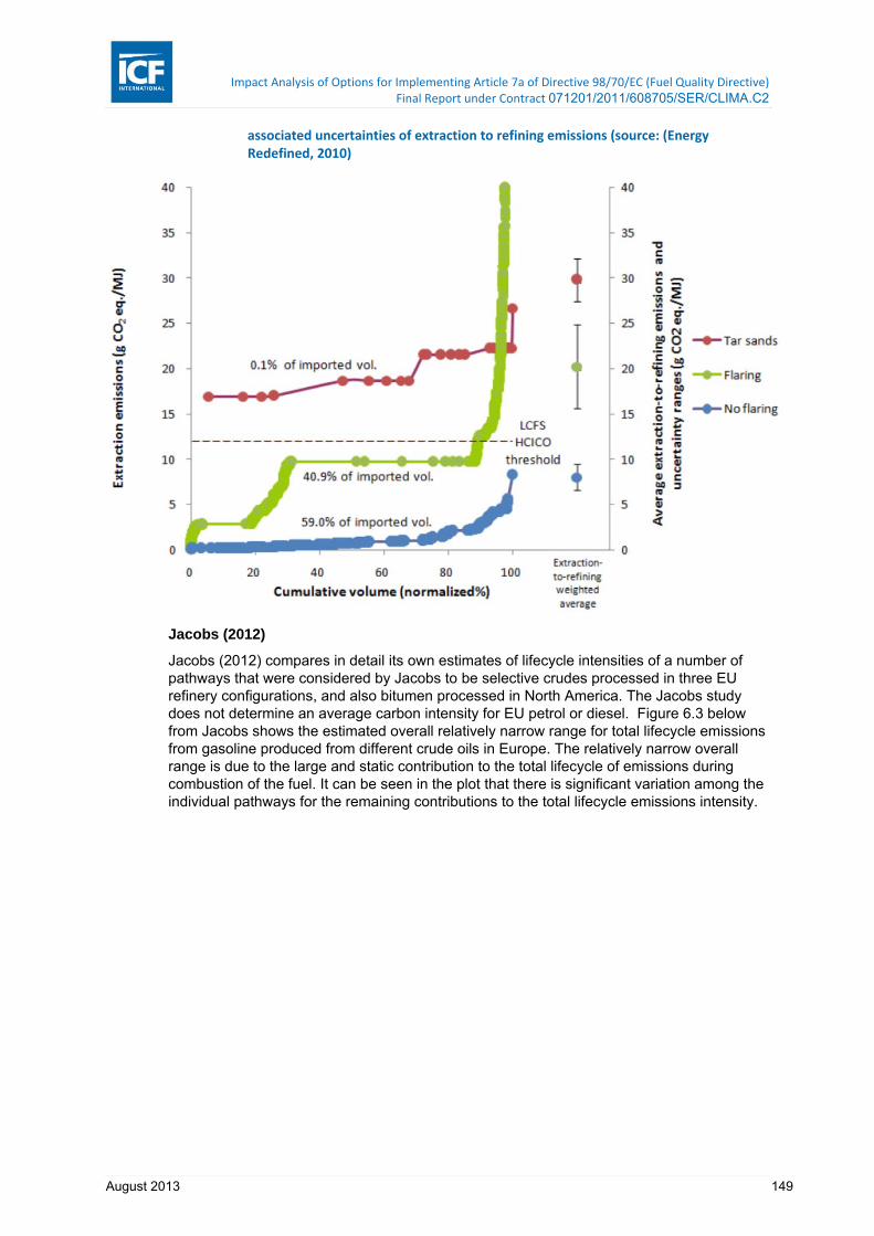
Impact Analysis of Options for Implementing Article 7a of Directive 98/70/EC (Fuel Quality Directive) Final Report under Contract 071201/2011/608705/SER/CLIMA.C2
August 2013 149
associated uncertainties of extraction to refining emissions (source: (Energy Redefined, 2010)
Jacobs (2012)
Jacobs (2012) compares in detail its own estimates of lifecycle intensities of a number of pathways that were considered by Jacobs to be selective crudes processed in three EU refinery configurations, and also bitumen processed in North America. The Jacobs study does not determine an average carbon intensity for EU petrol or diesel. Figure 6.3 below from Jacobs shows the estimated overall relatively narrow range for total lifecycle emissions from gasoline produced from different crude oils in Europe. The relatively narrow overall range is due to the large and static contribution to the total lifecycle of emissions during combustion of the fuel. It can be seen in the plot that there is significant variation among the individual pathways for the remaining contributions to the total lifecycle emissions intensity.

Impact Analysis of Options for Implementing Article 7a of Directive 98/70/EC (Fuel Quality Directive) Final Report under Contract 071201/2011/608705/SER/CLIMA.C2
August 2013 150
Figure 6.3 Lifecycle carbon Intensity of Producing Gasoline from Crude Oils to Europe (source: (Jacobs, 2012))
The Jacobs study selects specific lifecycle pathways to analyse, its estimates cannot be considered to fully represent the crudes that the EU consumes: a mapping exercise with the crudes forecast by the WORLD model for 2020 suggests that around one third of crudes can be matched to Jacob’s intensities when utilising specific crude names. The Jacobs study deviates from the approach in the JEC study for the refining emissions portion: three separate EU refining pathways, one Russian pathway and one US Gulf Coast diesel export refinery are assumed to be used and which are mapped to use of particular crudes. Whilst these may be more representative of actual emissions for those named refinery types (FCC visbreaking refinery, FCC coking refining, hydrocracking visbreaking refining, high conversion FCC coking refinery (US Gulf Coast) and hydroskimming refinery (Russia)), they do not necessarily reflect the production-weighted actual refining processes used in the EU for processing the entire EU crude slate.
6.2.3 Setting up the Analysis framework
Developing an EU dataset of suppliers
As identified earlier, the most suitable level of granularity for the analysis of impacts on suppliers is at the supplier level. A partial dataset has been gathered by the Commission to address this. The data gathered included fuel volumes (end fuels, i.e. with blends) supplied by a list of anonymous suppliers in select Member States. The data indicate that there is a wide range of size of suppliers, as shown in the two histograms below.

Impact Analysis of Options for Implementing Article 7a of Directive 98/70/EC (Fuel Quality Directive) Final Report under Contract 071201/2011/608705/SER/CLIMA.C2
August 2013 151
Figure 6.4 Histograms showing, for producers and traders separately, the breakdown by size of supplier (PJ/year total petrol and diesel) for 51 producers and 404 traders in the 12 Member States that responded to the 2010 questionnaire (data source: European Commission)
Figure 6.5 below plots the petrol/diesel split of suppliers against the normalised cumulative volume of total fuel supplied as reported by the 12 Member States. The plot includes both producers (around 60% of the fuel energy) and traders sequentially. The average size of the producers was much higher than that of traders, which is to be expected. The data suggest that suppliers have a wide range of petrol/diesel mixes.
Figure 6.5 Proportion of supply as petrol as a function of the normalised cumulative volume of total fuel supplied for 51 producers and 404 traders in the 12 Member States that responded to the 2010 questionnaire (data source: European Commission)
This analysis on the split of the petrol / diesel split across suppliers has been also undertaken at a more detailed level: specifically separating suppliers into size categories in order to assess the average petrol/diesel split and average supplier size at each size category. If this sub-analysis by supplier size category was not undertaken then the number of suppliers may be underestimated during extrapolation. The analysis of producers was

Impact Analysis of Options for Implementing Article 7a of Directive 98/70/EC (Fuel Quality Directive) Final Report under Contract 071201/2011/608705/SER/CLIMA.C2
August 2013 152
undertaken at three size categories due to the small number of producers. The analysis is summarised in Table 6.3 below. The analysis of traders was undertaken using six size categories in order to capture additional detail of the smaller traders. The analysis is summarised in Table 6.4 below.
Table 6.3 Analysis of data provided by 12 Member States of fuel producers (source: European Commission)
Size category of producer (TJ)
Number of producers in size
category
Average supplier size (petrol+diesel) (TJ/supplier)
Split of petrol supplied across
category (%)
Split of diesel supplied across
category (%)
0 - 10,000 14 1,380 0.5% 0.6%
10,000 - 100,000 17 35,561 14.9% 18.8%
100,000 - 1,000,000 20 143,470 84.7% 80.6%
Table 6.4 Analysis of data provided by 12 Member States of fuel traders (source: European Commission)
Size category of trader (TJ)
Number of traders in size
category
Average supplier size (petrol+diesel) (TJ/supplier)
Split of petrol supplied across
category (%)
Split of diesel supplied across
category (%)
0 – 10 60 2.0 0.002% 0.01%
10 - 100 77 80 0.23% 0.26%
100 - 1,000 112 217 0.5% 1.2%
1,000 - 10,000 84 5,246 22.6% 16.1%
10,000 - 100,000 69 25,049 64% 72%
100,000 - 1,000,000 2 133,802 13% 10%
The following steps have been taken in order to extrapolate the partial dataset from known Member States to be estimated to be fully representative of the EU27 (i.e. with ‘unknown Member States’ included):
1. For the known Member States, the number of refineries from European Commission (2010) has been mapped and matched to the number of producers, and from this an average ratio of producers/refineries was derived. This ratio was used to extrapolate the number of producers per Member State for the unknown Member States by using the data on the number of refineries in European Commission (2010).
2. The supply of petrol and diesel by producers reported by Member States was assessed against the refinery capacity data in European Commission (2010) and used to extrapolate estimates for the petrol and diesel supplied by producers in the unknown Member States.
i. The ratio of the reported supply of fuels by producers to the supply of fuels by traders was used to extrapolate the fuels supplied by traders in the unknown Member States.
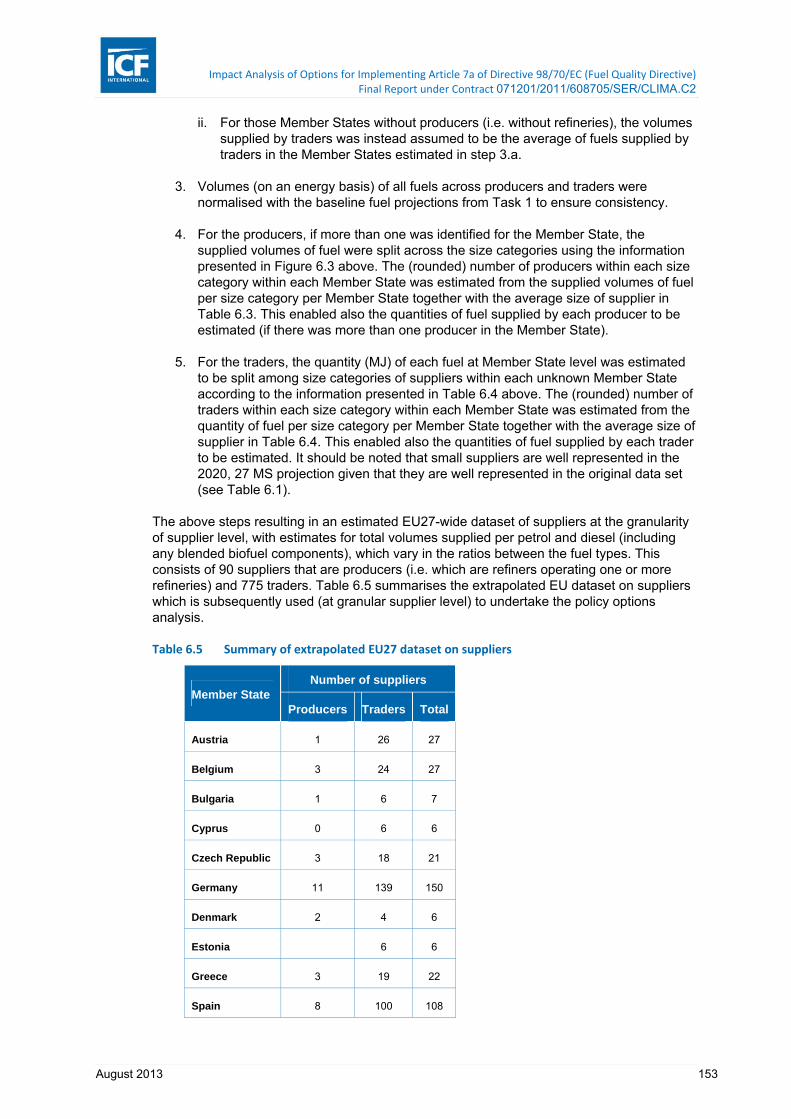
Impact Analysis of Options for Implementing Article 7a of Directive 98/70/EC (Fuel Quality Directive) Final Report under Contract 071201/2011/608705/SER/CLIMA.C2
August 2013 153
ii. For those Member States without producers (i.e. without refineries), the volumes supplied by traders was instead assumed to be the average of fuels supplied by traders in the Member States estimated in step 3.a.
3. Volumes (on an energy basis) of all fuels across producers and traders were normalised with the baseline fuel projections from Task 1 to ensure consistency.
4. For the producers, if more than one was identified for the Member State, the supplied volumes of fuel were split across the size categories using the information presented in Figure 6.3 above. The (rounded) number of producers within each size category within each Member State was estimated from the supplied volumes of fuel per size category per Member State together with the average size of supplier in Table 6.3. This enabled also the quantities of fuel supplied by each producer to be estimated (if there was more than one producer in the Member State).
5. For the traders, the quantity (MJ) of each fuel at Member State level was estimated to be split among size categories of suppliers within each unknown Member State according to the information presented in Table 6.4 above. The (rounded) number of traders within each size category within each Member State was estimated from the quantity of fuel per size category per Member State together with the average size of supplier in Table 6.4. This enabled also the quantities of fuel supplied by each trader to be estimated. It should be noted that small suppliers are well represented in the 2020, 27 MS projection given that they are well represented in the original data set (see Table 6.1).
The above steps resulting in an estimated EU27-wide dataset of suppliers at the granularity of supplier level, with estimates for total volumes supplied per petrol and diesel (including any blended biofuel components), which vary in the ratios between the fuel types. This consists of 90 suppliers that are producers (i.e. which are refiners operating one or more refineries) and 775 traders. Table 6.5 summarises the extrapolated EU dataset on suppliers which is subsequently used (at granular supplier level) to undertake the policy options analysis.
Table 6.5 Summary of extrapolated EU27 dataset on suppliers
Member State Number of suppliers
Producers Traders Total
Austria 1 26 27
Belgium 3 24 27
Bulgaria 1 6 7
Cyprus 0 6 6
Czech Republic 3 18 21
Germany 11 139 150
Denmark 2 4 6
Estonia 6 6
Greece 3 19 22
Spain 8 100 108

Impact Analysis of Options for Implementing Article 7a of Directive 98/70/EC (Fuel Quality Directive) Final Report under Contract 071201/2011/608705/SER/CLIMA.C2
August 2013 154
Member State Number of suppliers
Producers Traders Total
Finland 1 20 21
France 5 32 37
Hungary 8 20 28
Ireland 1 16 17
Italy 14 61 75
Lithuania 1 49 50
Luxembourg 0 11 11
Latvia 0 25 25
Malta 0 6 6
Netherlands 5 28 33
Poland 2 56 58
Portugal 2 18 20
Romania 5 5 10
Sweden 4 11 15
Slovenia 0 10 10
Slovakia 1 6 7
United Kingdom 9 53 62
EU27 total 90 775 865
Assumptions on apportionment of fuels across suppliers
The baseline from Task 1 of the various products and their feedstock origins and the total EU consumption need to be distributed across the suppliers identified in the supplier dataset. This process aims to capture the granularity of supplier level together with a possible reflection of the fuels and feedstock origins that suppliers in the EU may have. This is however a modelling exercise that, in the light of a lack of data reported by suppliers to date, cannot aim to accurately reflect all the fuel mixes that suppliers in the EU actually have. The aim through this exercise is to provide an indication of one possible distribution of fuels across the suppliers located in different Member States.
The main steps of this process include the following:
■ Establishing the split of each fuel pathway from the EU27 to the three WORLD model regions of Europe (and the associated Member States in each WORLD model region).
■ Further apportioning the subtotals across the applicable Member States utilising external datasets.
■ Splitting the Member State totals across the suppliers.
Impact Analysis of Options for Implementing Article 7a of Directive 98/70/EC (Fuel Quality Directive) Final Report under Contract 071201/2011/608705/SER/CLIMA.C2
August 2013 155
The first of these steps is a simple output from the Task 1 baseline modelling. The modelling identified that: petrol and diesel refined in EU from oil shale only occurs in the Member States in the WORLD Europe-East region; petrol/diesel refined in the EU from natural bitumen occurs only in the Member States of Europe-South, that diesel imports (including those derived from natural bitumen) are only imported to the Member States in WORLD model region Europe-North; and CTL/GTL is only produced in and imported to the Member States in WORLD model region Europe-North respectively.
The second step involves the assessment of external datasets in order to select a dataset that shows the most likely distribution across the Member States of the fuels in 2020 and to be aware of long term structural trends. The dataset of the IEA 2012 midterm forecast for 201770 was assessed, together with UNFCCC country for the reporting year 201071. The IEA dataset was selected in preference for the petrol and diesel apportioning across Member States due to its year of data being close to the 2020 base year. However, for LPG, the IEA dataset did not align with the UNFCCC reported values for LPG and, given that long-term infrastructure and demand for LPG in certain countries was not expected to change significantly, the UNFCCC reported values for LPG were instead adopted.72
Some small gap filling approaches were necessary in order to utilise the datasets of the IEA and the UNFCCC. The IEA dataset did not include forecasts for Latvia or Lithuania and consequently the UNFCCC dataset was used to infill for these Member States. Similarly, the UNFCCC dataset excludes Cyprus and so data from the IEA were used to in-fill for Cyprus.
This apportionment leads to the distribution of petrol, diesel (and their feedstock pathways) and LPG across the Member States as shown in the table on the following page.
70 Personal communication with IEA. 71 http://unfccc.int/national_reports/annex_i_ghg_inventories/national_inventories_submissions/items/6598.php 72 As recommended by the Commission.

Impact Analysis of Options for Implementing Article 7a of Directive 98/70/EC (Fuel Quality Directive) Final Report under Contract 071201/2011/608705/SER/CLIMA.C2
August 2013 156
Table 6.6 Distribution of petrol, diesel (and their feedstock pathways) and LPG across the Member States
Member State
Pet
rol
Co
nve
nti
on
al
refi
ned
in
EU
Pet
rol
Oil
Sh
ale
re
fin
ed i
n E
U
Pet
rol
Nat
ura
l B
itu
men
re
fin
ed i
n E
U
Pet
rol
To
tal
Die
sel
Co
nve
nti
on
al
refi
ned
in
EU
Die
sel
Co
nve
nti
on
al
imp
ort
ed U
SG
C
Die
sel
Co
nve
nti
on
al
imp
ort
ed R
uss
ia
Die
sel
Oil
sh
ale
re
fin
ed i
n E
U
Die
sel
Nat
ura
l b
itu
men
re
fin
ed i
n E
U
Die
sel
Nat
ura
l b
itu
men
im
po
rted
US
GC
Die
sel
CT
L
refi
ned
in
EU
Die
sel
GT
L
imp
ort
ed A
fric
a
Die
sel
To
tal
LP
G
To
tal
AT 52 0 0 52 86 7 70 0 0 1 1 3 167 1
BE 40 0 0 40 149 12 120 0 0 2 1 4 288 2
BG 10 0 0 10 46 0 0 0 0 0 0 0 47 15
CY 15 0 2 17 18 0 0 0 2 0 0 0 20 0
CZ 62 0 0 63 110 0 0 1 0 0 0 0 111 3
DE 619 0 0 619 617 50 497 0 0 6 6 19 1,196 21
DK 44 0 0 44 45 4 37 0 0 0 0 1 88 0
EE 10 0 0 10 20 0 0 0 0 0 0 0 20 0
EL 105 0 12 117 140 0 0 0 13 0 0 0 153 2
ES 149 0 17 166 754 0 0 0 69 0 0 0 824 1
FI 48 0 0 48 47 4 38 0 0 0 0 1 90 0
FR 199 0 0 199 558 46 450 0 0 6 5 17 1,081 5
HU 40 0 0 41 73 0 0 0 0 0 0 0 73 1
IE 45 0 0 45 38 3 30 0 0 0 0 1 73 0
IT 247 0 29 276 737 0 0 0 68 0 0 0 804 53
LT 8 0 0 8 33 0 0 0 0 0 0 0 33 7
LU 12 0 0 12 24 2 19 0 0 0 0 1 46 0
LV 8 0 0 8 25 0 0 0 0 0 0 0 25 1

Impact Analysis of Options for Implementing Article 7a of Directive 98/70/EC (Fuel Quality Directive) Final Report under Contract 071201/2011/608705/SER/CLIMA.C2
August 2013 157
Member State
Pet
rol
Co
nve
nti
on
al
refi
ned
in
EU
Pet
rol
Oil
Sh
ale
re
fin
ed i
n E
U
Pet
rol
Nat
ura
l B
itu
men
re
fin
ed i
n E
U
Pet
rol
To
tal
Die
sel
Co
nve
nti
on
al
refi
ned
in
EU
Die
sel
Co
nve
nti
on
al
imp
ort
ed U
SG
C
Die
sel
Co
nve
nti
on
al
imp
ort
ed R
uss
ia
Die
sel
Oil
sh
ale
re
fin
ed i
n E
U
Die
sel
Nat
ura
l b
itu
men
re
fin
ed i
n E
U
Die
sel
Nat
ura
l b
itu
men
im
po
rted
US
GC
Die
sel
CT
L
refi
ned
in
EU
Die
sel
GT
L
imp
ort
ed A
fric
a
Die
sel
To
tal
LP
G
To
tal
MT 3 0 0 3 16 0 0 0 1 0 0 0 17 0
NL 143 0 0 143 108 9 87 0 0 1 1 3 209 13
PL 136 1 0 137 359 0 0 2 0 0 0 0 361 73
PT 39 0 4 43 134 0 0 0 12 0 0 0 146 1
RO 52 0 0 52 119 0 0 1 0 0 0 0 120 1
SE 96 0 0 96 58 5 47 0 0 1 1 2 113 0
SI 21 0 2 24 47 0 0 0 4 0 0 0 51 0
SK 20 0 0 20 43 0 0 0 0 0 0 0 43 1
UK 430 0 0 430 329 27 265 0 0 3 3 10 637 5
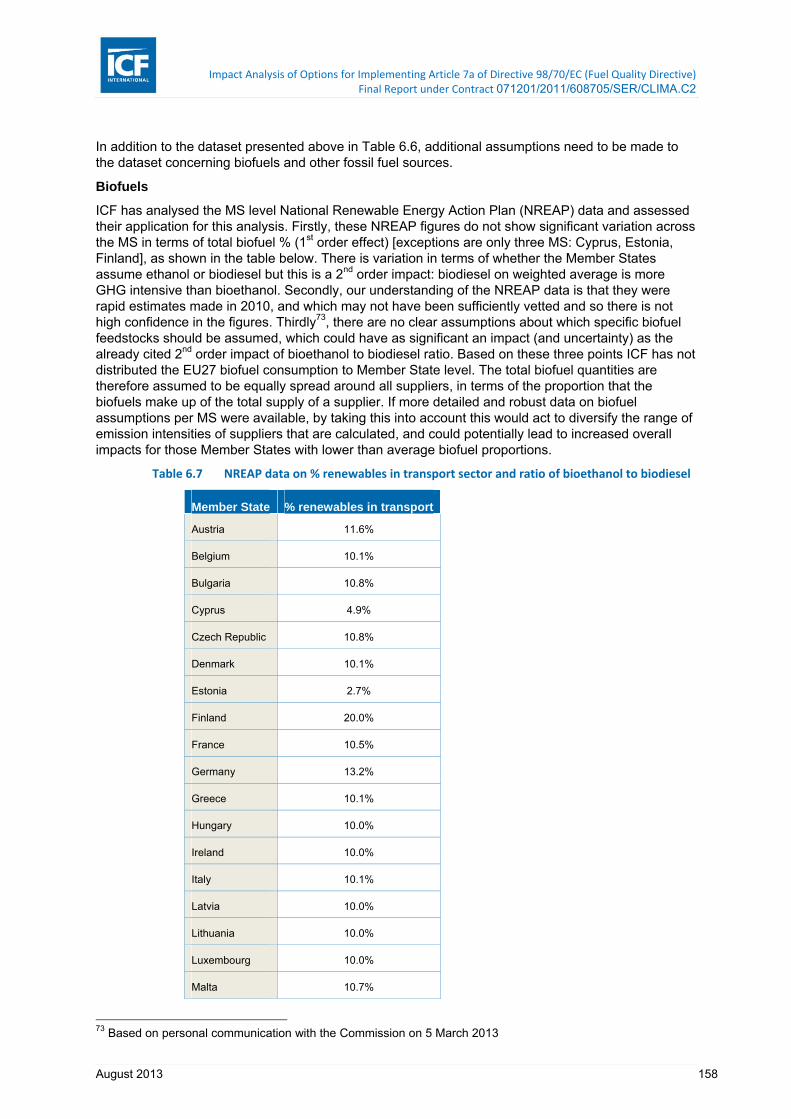
Impact Analysis of Options for Implementing Article 7a of Directive 98/70/EC (Fuel Quality Directive) Final Report under Contract 071201/2011/608705/SER/CLIMA.C2
August 2013 158
In addition to the dataset presented above in Table 6.6, additional assumptions need to be made to the dataset concerning biofuels and other fossil fuel sources.
Biofuels
ICF has analysed the MS level National Renewable Energy Action Plan (NREAP) data and assessed their application for this analysis. Firstly, these NREAP figures do not show significant variation across the MS in terms of total biofuel % (1st order effect) [exceptions are only three MS: Cyprus, Estonia, Finland], as shown in the table below. There is variation in terms of whether the Member States assume ethanol or biodiesel but this is a 2nd order impact: biodiesel on weighted average is more GHG intensive than bioethanol. Secondly, our understanding of the NREAP data is that they were rapid estimates made in 2010, and which may not have been sufficiently vetted and so there is not high confidence in the figures. Thirdly73, there are no clear assumptions about which specific biofuel feedstocks should be assumed, which could have as significant an impact (and uncertainty) as the already cited 2nd order impact of bioethanol to biodiesel ratio. Based on these three points ICF has not distributed the EU27 biofuel consumption to Member State level. The total biofuel quantities are therefore assumed to be equally spread around all suppliers, in terms of the proportion that the biofuels make up of the total supply of a supplier. If more detailed and robust data on biofuel assumptions per MS were available, by taking this into account this would act to diversify the range of emission intensities of suppliers that are calculated, and could potentially lead to increased overall impacts for those Member States with lower than average biofuel proportions.
Table 6.7 NREAP data on % renewables in transport sector and ratio of bioethanol to biodiesel
Member State % renewables in transport
Austria 11.6%
Belgium 10.1%
Bulgaria 10.8%
Cyprus 4.9%
Czech Republic 10.8%
Denmark 10.1%
Estonia 2.7%
Finland 20.0%
France 10.5%
Germany 13.2%
Greece 10.1%
Hungary 10.0%
Ireland 10.0%
Italy 10.1%
Latvia 10.0%
Lithuania 10.0%
Luxembourg 10.0%
Malta 10.7%
73 Based on personal communication with the Commission on 5 March 2013

Impact Analysis of Options for Implementing Article 7a of Directive 98/70/EC (Fuel Quality Directive) Final Report under Contract 071201/2011/608705/SER/CLIMA.C2
August 2013 159
Member State % renewables in transport
Netherlands 10.3%
Poland 10.1%
Portugal 10.0%
Romania 10.0%
Slovakia 10.0%
Slovenia 10.5%
Spain 13.6%
Sweden 13.8%
United Kingdom 10.3%
Other fuels
Regarding the distribution of CNG across Member States, the UNFCCC data on reported use of gaseous fuels in transport appeared to be both patchy in coverage and internally inconsistent, such that the dataset were deemed insufficiently robust to be used for apportioning data across Member States. Therefore all suppliers were assumed to have the same (small) percentage of CNG in their fuel mix. This simplification for the purposes of modelling reduces the potential granularity that suppliers’ actual values may exhibit. In reality, CNG suppliers may actually be specialist suppliers that may not also supply conventional petrol and diesel products. As such these suppliers may incur higher impacts which this analysis does not capture.
Similarly to biofuels and CNG, no Member State distribution of hydrogen and electricity other than an even fractional distribution for each supplier was adopted.
Distribution of GHG intensities of Refinery Feedstocks
Conventional crudes refined in the EU
Following the review above of literature on the GHG intensities of different crudes, in order to match the objective of ensuring the most complete coverage of crudes refined in the EU and consistent approach to the European Commission proposed default values, the data source selected to represent supplier-specific intensities is the JEC study, and its underpinning data. The underpinning data concern country-specific flaring and venting intensities of crudes. In order to apply these data from JEC, ICF has undertaken the following process
1. Undertake a mapping exercise between the crude countries of origin listed in Table 3.3.1-3 of JEC (2011) and the crudes identified in the WORLD model as being consumed in the EU in 2020, excluding the two unconventional crudes.74
2. The upstream intensity for each country of origin is taken as the sum of production and flaring/venting, which is production weighted, and then scaled to the production weighted mean of upstream intensity for conventional crudes for the separate petrol and diesel intensities.
a. The production intensity is a fixed value for all crude origin countries of 2.3 gCO2e/MJ.
74 All EU countries not specifically listed in JEC were mapped to ‘Other EU’. All four North Sea crudes from the WORLD model were mapped to ‘UK’. Where multiple crudes in the WORLD model exist for one country in the JEC study, they are each mapped to that one country. The WORLD model crudes mapped to ‘Others’ in the JEC table are BENIN, GABON GAMBA, ZAIRE and TURKMENISTAN CHELEKAN (totalling 2.7% of EU crude input).

Impact Analysis of Options for Implementing Article 7a of Directive 98/70/EC (Fuel Quality Directive) Final Report under Contract 071201/2011/608705/SER/CLIMA.C2
August 2013 160
b. The flaring and venting GHG intensity for each country of crude origin is taken from a combination of the JEC-quoted results for both oil and oil&gas flaring and venting at country level.75.
c. The total production and flaring/venting is then weighted according to the EU27 crude mix from year 201076 to give a total EU upstream intensity (which is not separated by product).
d. Each country of origin’s intensity is scaled by the ratio of the weighted average in part c. to the upstream intensities for petrol and diesel proposed by the Commission (2011).
3. The sum GHG intensity for the lifecycle stages of transport, refining, distribution and combustion is taken from the difference between the EC proposal values for upstream and lifecycle intensity.
4. The total lifecycle intensity is the sum of points 2 and 3.
The above steps led to the upstream intensities for the countries of crude origin from JEC (2011) as shown in Table 6.8. The total lifecycle intensities, plotted as a function of the 2020 crude mix and including unconventional sources, are shown in Figure 6.6. The intensities are distributed over a narrow range as per the majority of the crudes identified above in Brandt (2011).
Table 6.8 Development of upstream GHG intensities (gCO2e/MJ) for petrol and diesel derived from conventional crudes (source: based on JEC, 2011)
Crude origin Relevance in EU27
crude mix 2010
Crude production
(g/MJ crude)
F&V (g/MJ crude)
Total upstream intensity
(g/MJ crude)
Total upstream
intensity for petrol (g/MJ
petrol)
Total upstream
intensity for diesel (g/MJ
diesel)
Russia 28% 2.3 3.92 6.22 6.05 6.16
Norway 13% 2.3 0.16 2.46 2.39 2.44
Libya 10% 2.3 2.81 5.11 4.97 5.07
UK 5% 2.3 0.85 3.15 3.06 3.12
Saudi Arabia 6% 2.3 0.44 2.74 2.67 2.72
Iran 5% 2.3 2.75 5.05 4.91 5.01
Nigeria 4% 2.3 8.73 11.03 10.73 10.93
Kazakhstan 6% 2.3 4.22 6.52 6.34 6.46
Iraq 3% 2.3 4.10 6.40 6.23 6.35
Azerbaijan 4% 2.3 0.57 2.87 2.79 2.84
Angola 1% 2.3 2.35 4.65 4.53 4.61
Algeria 1% 2.3 3.20 5.50 5.35 5.45
Denmark 1% 2.3 0.57 2.87 2.79 2.85
Other EU 0% 2.3 0.45 2.75 2.68 2.73
75 JEC adopted an EU-wide GHG intensity for venting and flaring of 2.5gCO2e/MJ, which lies between the oil only F/V intensity of 3.2gCo2e/MJ and the oil & gas F/V intensity of 2gCO2e/MJ. 76 Reference: Table 2.23 in the Task 1 report.

Impact Analysis of Options for Implementing Article 7a of Directive 98/70/EC (Fuel Quality Directive) Final Report under Contract 071201/2011/608705/SER/CLIMA.C2
August 2013 161
Venezuela 1% 2.3 1.22 3.52 3.43 3.49
Mexico 1% 2.3 0.99 3.29 3.20 3.26
Syria 1% 2.3 2.77 5.07 4.93 5.02
Kuwait 1% 2.3 0.88 3.18 3.09 3.15
Egypt 1% 2.3 1.90 4.20 4.08 4.16
Brazil 1% 2.3 0.79 3.09 3.01 3.06
Others 6% 2.3 8.03 10.33 10.05 10.24
EU weighted average 5.35 5.2 5.3
After completing the steps outlined above, the assumed GHG life cycle intensities of the crudes and the petrol/diesel produced in the EU are listed in the table below.
Table 6.9 Assumed GHG intensities (gCO2e/MJ) for petrol and diesel derived from conventional crudes assumed to be used in the EU in 2020 (source: this study)
Crude region
Crude Upstream
Transport, refining, distribution and
combustion Total life cycle
Petrol Diesel Petrol Diesel Petrol Diesel
European
Crudes
AUSTRIA 2.7 2.7 82.3 83.8 85.0 86.5
DENMARK 2.8 2.8 82.3 83.8 85.1 86.6
EASTERN EUROPE 2.7 2.7 82.3 83.8 85.0 86.5
NORTH SEA CONDENSATE 3.1 3.1 82.3 83.8 85.4 86.9
NORTH SEA HITAN HVY SWT 3.1 3.1 82.3 83.8 85.4 86.9
NORTH SEA LIGHT SOUR 3.1 3.1 82.3 83.8 85.4 86.9
NORTH SEA LIGHT SWEET
(BRENT) 3.1 3.1 82.3 83.8 85.4 86.9
FRANCE 2.7 2.7 82.3 83.8 85.0 86.5
W. GERMANY 2.7 2.7 82.3 83.8 85.0 86.5
GREECE 2.7 2.7 82.3 83.8 85.0 86.5
NETHERLANDS 2.7 2.7 82.3 83.8 85.0 86.5
NORWAY 2.4 2.4 82.3 83.8 84.7 86.2
ITALY 2.7 2.7 82.3 83.8 85.0 86.5
SPAIN 2.7 2.7 82.3 83.8 85.0 86.5
TURKEY 2.7 2.7 82.3 83.8 85.0 86.5
NORTH
AFRICAN
CRUDES
ALGERIAN CONDENSATE 5.3 5.5 82.3 83.8 87.6 89.3
ALGERIAN SAHARAN 5.3 5.5 82.3 83.8 87.6 89.3
EGYPT SUEZ BLEND 4.1 4.2 82.3 83.8 86.4 88.0
LIBYAN 5.0 5.1 82.3 83.8 87.3 88.9
WEST
AFRICAN
CRUDES
ANGOLA 4.5 4.6 82.3 83.8 86.8 88.4
ANGOLA HITAN (KUITO) 4.5 4.6 82.3 83.8 86.8 88.4
BENIN 10.0 10.2 82.3 83.8 92.3 94.0
GABON GAMBA 10.0 10.2 82.3 83.8 92.3 94.0
NIGERIAN BONNY/LIGHT 10.7 10.9 82.3 83.8 93.0 94.7

Impact Analysis of Options for Implementing Article 7a of Directive 98/70/EC (Fuel Quality Directive) Final Report under Contract 071201/2011/608705/SER/CLIMA.C2
August 2013 162
Crude region
Crude Upstream
Transport, refining, distribution and
combustion Total life cycle
Petrol Diesel Petrol Diesel Petrol Diesel
NIGERIAN BRASS RIVER/
ESCRAVOS/QUA IBOE 10.7 10.9 82.3 83.8 93.0 94.7
NIGERIAN OKONO ETC LIGHT 10.7 10.9 82.3 83.8 93.0 94.7
ZAIRE 10.0 10.2 82.3 83.8 92.3 94.0
CASPIAN AZERBAIJAN AIOC 2.8 2.8 82.3 83.8 85.1 86.6
TURKMENISTAN CHELEKAN 10.0 10.2 82.3 83.8 92.3 94.0
FSU RUSSIA URALS 6.0 6.2 82.3 83.8 88.3 90.0
MIDDLE
EASTERN
CRUDES
IRAQ BASRAH 6.2 6.3 82.3 83.8 88.5 90.1
IRAQ KIRKUK 6.2 6.3 82.3 83.8 88.5 90.1
IRANIAN HVY SOUR (AZADEGAN) 4.9 5.0 82.3 83.8 87.2 88.8
SAUDI ARABIAN HEAVY 2.7 2.7 82.3 83.8 85.0 86.5
SAUDI ARABIAN LIGHT 2.7 2.7 82.3 83.8 85.0 86.5
CARIBBEAN
& LATIN
AMERICAN
VENEZUELAN SYNCRUDE 3.4 3.5 82.3 83.8 85.7 87.3
VENEZ XHVY(BOSCAN) 3.4 3.5 82.3 83.8 85.7 87.3
VENEZ HEAVY(BACH LT) 3.4 3.5 82.3 83.8 85.7 87.3
It is important to note that the intensities that have been applied to the 2020 conventional crude mix are consistent with the 2010 default unit intensities proposed by the Commission in the Proposal. However once the intensities have been applied to the projected 2020 crude mix to obtain absolute emissions estimates (i.e. under supplier-specific approaches), this will not strictly speaking be consistent with the 2020 crude mix being multiplied by the 2010 default unit intensities given that the 2010 default unit intensities were derived on the basis of the 2010 crude slate. As such, small revisions to the default unit intensities are set out in the next section.
Intensities of imported conventional diesel
In addition to the diesel refined in the EU, the EU is also an importer of diesel. The 2020 fuel projections forecast that this diesel deficit will primarily be met through imports from Russia and to a lesser extent the US and Canada.77
Under policy options 1 and 3 (opt in), these imported products will not be differentiated against other EU-refined products, and so the assumed intensities are those as per the EC’s proposed values from October 2011.
Under the supplier specific policy options (i.e. including option 3 opt out), there is a need to make an assumption regarding the GHG intensity for these imports. In this regard, the diesel imports from Russia have been assumed to have the same carbon intensity as listed against ‘Russian Urals’ in Table 6.9 above, i.e. assuming that diesel produced in Russian is derived from Russian origin crude, and that that diesel refined in the EU from Russian crude has the same intensity as diesel refined in Russia. Due to a lack of specific information regarding the conventional feedstocks of US Gulf Coast refineries, the diesel imports from the US gulf coast are assumed to have the carbon intensity as per the Commission’s proposals. Hence,
77 In line with the Task 1 baseline analysis, a portion of the volumes of imports from the US/Canada are assumed to be derived from natural bitumen (see below) and consequently have been assigned the unit GHG intensities for this feedstock category from the European Commission (2011)

Impact Analysis of Options for Implementing Article 7a of Directive 98/70/EC (Fuel Quality Directive) Final Report under Contract 071201/2011/608705/SER/CLIMA.C2
August 2013 163
regional variation in refinery emissions were not considered in the subsequent analysis of options.
Table 6.10 Assumed GHG intensities (gCO2/MJ) for imported diesel derived from conventional crude under policy options 1 and 3 (opt in)
Source Refinery origin
Feedstock category
Policy options 1 and 3 (opt in) Policy option 3 (opt out)
Upstream
Transport, refining,
distribution and
combustion
Life cycle Upstream
Transport, refining,
distribution and
combustion
Life cycle
Imported Russia Conventional 5.3 83.8 89.1 6.2 83.8 90.0
Imported US Gulf
Coast Conventional 5.3 83.8 89.1 5.3 83.8 89.1
Intensities of unconventional feedstocks
No deviation from the EC’s proposed intensities for unconventional feedstocks is assumed in this analysis. The original values have been assumed, and are shown in the table below.
During the course of this study, stakeholders have raised objections to the use of the default values (specifically: diesel produced from oil shale is not supported by the Estonian authorities who have provided a background document to estimate an alternative carbon intensity value), but it was outside the scope of this work to revisit the Commission’s default values.
Table 6.11 Assumed GHG intensities (gCO2/MJ) for petrol and diesel derived from unconventional crudes under policy options 1 and 3 (opt in and opt out)
Refined or imported
Refinery origin
Feedstock category
Upstream Transport, refining,
distribution and combustion
Life cycle
Petrol Diesel Petrol Diesel Petrol Diesel
Refined in EU EU CTL N/A 100 N/A 72 N/A 172
Refined in EU EU Natural bitumen 24.7 24.7 82.3 83.8 107.0 108.5
Refined in EU EU Oil shale 49 49 82.3 84.7 131.3 133.7
Imported US Gulf Coast Natural bitumen N/A 24.7 N/A 83.8 N/A 108.5
Imported Africa GTL N/A 25 N/A 72 N/A 97
Taking into account all of the feedstocks imported to the EU, the figure below plots the resulting lifecycle GHG intensities for both conventional and unconventional crudes projected to enter the EU for refining into FQD products in 2020 by the WORLD model.
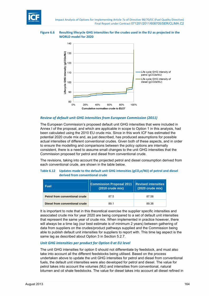
Impact Analysis of Options for Implementing Article 7a of Directive 98/70/EC (Fuel Quality Directive) Final Report under Contract 071201/2011/608705/SER/CLIMA.C2
August 2013 164
Figure 6.6 Resulting lifecycle GHG intensities for the crudes used in the EU as projected in the WORLD model for 2020
Review of default unit GHG intensities from European Commission (2011)
The European Commission’s proposed default unit GHG intensities that were included in Annex I of the proposal, and which are applicable in scope to Option 1 in this analysis, had been calculated using the 2010 EU crude mix. Since in this work ICF has estimated the potential 2020 crude mix and, as just described, has produced assumptions for possible actual intensities of different conventional crudes. Given both of these aspects, and in order to ensure the modelling and comparisons between the policy options are internally consistent, there is a need to assume small changes to the unit GHG intensities that the Commission proposed for petrol and diesel from conventional crude.
The revisions, taking into account the projected petrol and diesel consumption derived from each conventional crude, are shown in the table below.
Table 6.12 Updates made to the default unit GHG intensities (gCO2e/MJ) of petrol and diesel derived from conventional crude
Fuel Commission Proposal 2011
(2010 crude mix) Revised intensities
(2020 crude mix)
Petrol from conventional crude 87.5 87.58
Diesel from conventional crude 89.1 89.38
It is important to note that in this theoretical exercise the supplier specific intensities and associated crude mix for year 2020 are being compared to a set of default unit intensities that represent the same year of crude mix. When implemented in practice however, there will always be a time lag (our best estimate is of minimum 2 years) between gathering of data from suppliers on the crudes/product pathways supplied and the Commission being able to publish default unit intensities for suppliers to report with. This time lag aspect is the same lag as described about Option 3 in Section 5.2.7.
Unit GHG intensities per product for Option 0 at EU level
The unit GHG intensities for option 0 should not differentiate by feedstock, and must also take into account all the different feedstocks being utilised. Based on the process undertaken above to update the unit GHG intensities for petrol and diesel from conventional fuels, the default unit intensities were also developed for petrol and diesel. The value for petrol takes into account the volumes (MJ) and intensities from conventional, natural bitumen and oil shale feedstocks. The value for diesel takes into account all diesel refined in
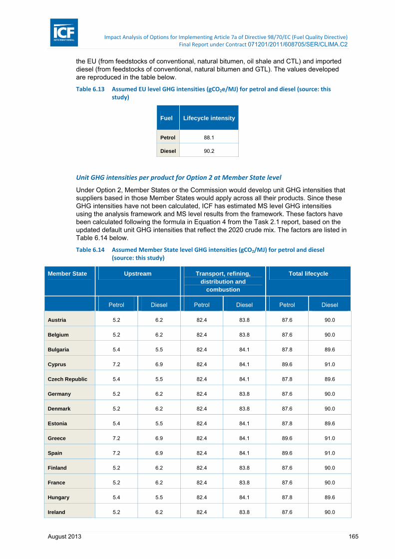
Impact Analysis of Options for Implementing Article 7a of Directive 98/70/EC (Fuel Quality Directive) Final Report under Contract 071201/2011/608705/SER/CLIMA.C2
August 2013 165
the EU (from feedstocks of conventional, natural bitumen, oil shale and CTL) and imported diesel (from feedstocks of conventional, natural bitumen and GTL). The values developed are reproduced in the table below.
Table 6.13 Assumed EU level GHG intensities (gCO2e/MJ) for petrol and diesel (source: this study)
Fuel Lifecycle intensity
Petrol 88.1
Diesel 90.2
Unit GHG intensities per product for Option 2 at Member State level
Under Option 2, Member States or the Commission would develop unit GHG intensities that suppliers based in those Member States would apply across all their products. Since these GHG intensities have not been calculated, ICF has estimated MS level GHG intensities using the analysis framework and MS level results from the framework. These factors have been calculated following the formula in Equation 4 from the Task 2.1 report, based on the updated default unit GHG intensities that reflect the 2020 crude mix. The factors are listed in Table 6.14 below.
Table 6.14 Assumed Member State level GHG intensities (gCO2/MJ) for petrol and diesel (source: this study)
Member State Upstream Transport, refining, distribution and
combustion
Total lifecycle
Petrol Diesel Petrol Diesel Petrol Diesel
Austria 5.2 6.2 82.4 83.8 87.6 90.0
Belgium 5.2 6.2 82.4 83.8 87.6 90.0
Bulgaria 5.4 5.5 82.4 84.1 87.8 89.6
Cyprus 7.2 6.9 82.4 84.1 89.6 91.0
Czech Republic 5.4 5.5 82.4 84.1 87.8 89.6
Germany 5.2 6.2 82.4 83.8 87.6 90.0
Denmark 5.2 6.2 82.4 83.8 87.6 90.0
Estonia 5.4 5.5 82.4 84.1 87.8 89.6
Greece 7.2 6.9 82.4 84.1 89.6 91.0
Spain 7.2 6.9 82.4 84.1 89.6 91.0
Finland 5.2 6.2 82.4 83.8 87.6 90.0
France 5.2 6.2 82.4 83.8 87.6 90.0
Hungary 5.4 5.5 82.4 84.1 87.8 89.6
Ireland 5.2 6.2 82.4 83.8 87.6 90.0

Impact Analysis of Options for Implementing Article 7a of Directive 98/70/EC (Fuel Quality Directive) Final Report under Contract 071201/2011/608705/SER/CLIMA.C2
August 2013 166
Member State Upstream Transport, refining, distribution and
combustion
Total lifecycle
Petrol Diesel Petrol Diesel Petrol Diesel
Italy 7.2 6.9 82.4 84.1 89.6 91.0
Lithuania 5.4 5.5 82.4 84.1 87.8 89.6
Luxembourg 5.2 6.2 82.4 83.8 87.6 90.0
Latvia 5.4 5.5 82.4 84.1 87.8 89.6
Malta 7.2 6.9 82.4 84.1 89.6 91.0
Netherlands 5.2 6.2 82.4 83.8 87.6 90.0
Poland 5.4 5.5 82.4 84.1 87.8 89.6
Portugal 7.2 6.9 82.4 84.1 89.6 91.0
Romania 5.4 5.5 82.4 84.1 87.8 89.6
Sweden 5.2 6.2 82.4 83.8 87.6 90.0
Slovenia 7.2 6.9 82.4 84.1 89.6 91.0
Slovakia 5.4 5.5 82.4 84.1 87.8 89.6
United Kingdom 5.2 6.2 82.4 83.8 87.6 90.0
6.2.3.2 Methodology for determining Option 3 supplier choices
As described in the policy options descriptions section of the Task 2.1 report, suppliers would be expected to choose whether to opt in or opt out of Option 3 by estimating which route would be beneficial to them in terms of reducing their deficit against the FQD reduction target. I.e. if choosing to opt out would actually lead to lower total GHG intensity for the supplier if their supply chain is less carbon intensive than the average set on basis of the default unit GHG factors, then the supplier would do so. The option 3 opt in default values would initially be set to the values under Option 1, but would then be recalculated at a later date and set in advance in order to limit uncertainty to investors.
Therefore in order to model this supplier decision making process, the analysis framework has made a comparison for each supplier of what the emissions intensity would be under Option 1 with that which would be obtained by assuming ‘actual emissions intensity’ (under option 5) using the crude-specific values set out in the section above titled Distribution of GHG intensities of Refinery Feedstocks on page 159. This analysis is therefore based on the first year of iteration of Option 3 since in a second period of iteration the opt in default unit GHG intensities would differ from those under Option 1. If the supplier would stand to benefit from the use of the assumed actual emissions intensities then these are applied and the supplier is marked as being opted out.
This modelling of supplier decision making has not however taken into account the additional MRV costs that a supplier would incur in developing the supplier specific data. Estimated costs for this are outlined later in this section. If the additional costs of developing supplier specific data were taken into account, this would effectively decrease the number of suppliers opting out. The amount that this would decrease would be related to the potential

Impact Analysis of Options for Implementing Article 7a of Directive 98/70/EC (Fuel Quality Directive) Final Report under Contract 071201/2011/608705/SER/CLIMA.C2
August 2013 167
compliance costs of implementing abatement measures since this would be the alternative that a supplier would need to undertake.
For subsequent years of iteration, in which the unit GHG intensities have been adjusted from the initial position, the number of suppliers opting out would increase.
6.2.4 Identification of compliance measures and supplier decision making
Suppliers that need to reduce their GHG intensity to meet the FQD will opt for the most cost efficient method to do so. Whether this is to pool with (an)other supplier(s), as provided for under Article 7a(4) of the FQD, through coming to a negotiated cost with (an)other supplier(s), or if this is to implement emission reduction options as the suppliers themselves, the supplier will choose to implement the most cost efficient measure.
Depending on the policy option being considered, some abatement measures that reduce the assumed actual emissions of a supplier will effectively make no difference to the calculation of the supplier’s GHG intensity due to the methodology of the Options. The abatement measures that may be available to suppliers, depending on the policy option being assessed, are described in more detail in the following subsections, and include the following:
■ Upstream emission reductions (UER). Whilst the description ‘upstream emission reduction’ could constitute a range of emission reduction measures that could be taken upstream of the refinery, i.e. at the extraction / crude production stage, in this section UERs are interpreted and costed as reductions in upstream flaring practices. This is therefore not representative of possibilities for refineries to reduce any flaring practices.
■ Feedstock Selecting:
– Selecting among feedstock categories – Since the existing Commission proposal (i.e. policy option 1 under this report) classifies feedstocks into a number of different categories and assigns life cycle greenhouse gas intensities for each of these feedstock categories, a supplier could choose to select feedstocks from one category over another category. For example, selecting conventional crudes over unconventional feedstocks such as natural bitumen or oil shale.
– Selecting among any crudes – Under policy options 3 and 5 that provides the possibility for supplier-specific GHG intensities to be developed as opted out suppliers, suppliers could, in principle, choose a measure to select among [any] crudes if an alternative crude will reduce their total life cycle GHG intensity. The permitted level of disaggregation (i.e. whether crudes are grouped by oil field, trade name, or some other feedstock categories) depends on the soundness of the calculation method used to estimate the GHG emissions from all groupings of crudes. In general heavier crudes require more processing, and thus exhibit higher GHG emission intensities, also the more cracking and complex a refinery the higher GHG emission intensities.
■ Additional blending with biofuels. The baseline includes certain proportions of biofuels (bioethanol and biodiesels) blended within the supplied fuels, i.e. blending which meets the existing requirements of the Renewable Energy Directive (RED). Suppliers could implement a measure to increase the blended proportion of biofuels (if the biofuel displaces a fuel with a higher GHG intensity), i.e. undertake additional blending.
■ Selecting imported products. For products originating from refineries that process high carbon feedstocks, these products if imported to the EU under option 1, 3 or 5 would be classified on basis of the respective feedstock categories. The importer could instead switch to importing the same product but which is derived from lower GHG feedstocks.
■ Selecting refining products in the EU over imported products. If such imports were in lieu of in-EU refining and supply of finished products, then either reduced EU refinery capacity utilisation would ensue or refinery closures may occur.

Impact Analysis of Options for Implementing Article 7a of Directive 98/70/EC (Fuel Quality Directive) Final Report under Contract 071201/2011/608705/SER/CLIMA.C2
August 2013 168
It should be noted that any option related to products excludes selecting one type of fuel over another (e.g., LPG over diesel or petrol). Such selection could not be induced by a carbon price premium resulting from the FQD requiring compliance in 2020 as drivers for switching between fuels materialise over a longer time horizon stemming from long-term drivers such as changes to vehicle fleets and/or taxation regimes.
In summary, the abatement measures most attractive to the supplier under different policy options being considered are overviewed in Table 6.15.
Table 6.15 Abatement choices for suppliers
Policy option
Additional biofuel
blending
Upstream emission
reductions
Crude Selection Product Selection
EU refinery switch
feedstock categories
EU refinery switch
among any crude
feedstock
Import products
refined from other
feedstock categories
Import products
refined from any crude feedstock
Option 0
Option 1
Option 2
Option
3
Opt
in
Opt
out
() ()
Option 5 () ()
Note: product selection excludes migration from CTL-derived diesel for other diesel and migration from conventional CNG and
LPG to other CNG and LPG feedstocks.
Electric vehicles as a measure for compliance is available under all policy options. Electric vehicles has not been assessed further as a realistic compliance option in this analysis due to the low perceived cost effectiveness which would effectively preclude its implementation when more cost effective alternatives exist. However uptake of electric vehicles enhanced by other legislative measures has been reflected in the projected 2020 energy demand.
In addition, for those policy options in which the supplier is reporting actual supplier specific intensities, any measure that reduces the GHG intensity of that supplier’s product would be available to the supplier. This could include for example refinery optimisation or changes to transport/distribution efficiencies. Such measures are not considered further here because the measures listed in the table above are considered those likely to be most attractive to suppliers, and further that refinery emissions intensity reduction is already covered within the scope of the EU ETS and that transport/distribution emission reduction projects are likely to affect total lifecycle intensities only marginally. The emission intensities assumed for supplier specific emissions methods do not assume any specific refinery emission savings.
6.2.4.2 Upstream emission reductions (flare reductions)
As described in Task 1.3, flare reduction projects have previously been implemented and their costs and effectiveness have been reviewed and summarised in Task 1.3. Flaring currently constitutes a wide ranging, and in some cases significant, proportion of total life cycle GHG intensities. Brandt (2011) estimated that the weighted average upstream GHG emissions intensity was 4.8g/MJ crude. Figure 6.1 and Figure 6.2 above showed wide variation in the upstream emissions when separated by country of crude origin. This

Impact Analysis of Options for Implementing Article 7a of Directive 98/70/EC (Fuel Quality Directive) Final Report under Contract 071201/2011/608705/SER/CLIMA.C2
August 2013 169
variation is due to both differences in extraction and flaring emissions, and we assess the majority of the variation to be due to flaring practices. JEC (2011) also showed considerable emissions intensity variation across crude countries of origin.
The cost effectiveness of flare reduction, as described in Task 1.3 have been based on those existing flare reduction projects that have been previously certified under CDM and have occurred within the past decade. Whilst the cost effectiveness that has been derived is based on the most robust data available that can be used for this purpose, it may be the case that the projects undertaken to date on flare reduction have been those which are the most cost-effective to a certain degree. As such, future flare reduction projects may not necessarily have the same cost-effectiveness. In essence this suggests the possibility that the flare reduction cost-effectiveness presented could be an underestimate of the actual costs that might be incurred. Nevertheless, it is expected that projects of similar size and cost could be implemented between 2010 and 2020, particularly as the go-ahead of projects under CDM is sensitive to a number of other factors beyond cost-effectiveness (e.g. administrative, political, technical etc.).
The costs that have been developed are in effect quantised: they are associated with specific projects. Whilst future projects may be in different quanta (associated with different flare reduction projects), these same costs, abatement potential and consequent cost effectiveness have been assumed to remain valid for the next decade, in the absence of alternative data.
Flare reduction projects, which have had their effectiveness fully verified through verification processes under the CDM or other routes, offer suppliers tangible emission reductions from a global perspective.
Some potential implementation issues associated with flare reduction projects and compatibility with options are established in Section 6.2.6. This was an issue to do with supplier specific GHG intensities. Legislators will need to be careful not to allow double counting of any UER projects that have already been claimed. This therefore requires an additional administrative step (centralized dataset on projects claimed by suppliers) to be referred to by all suppliers calculating their own intensities, as well as potentially creating a difficulty for suppliers to calculate their actual intensities since this could require them to estimate what their intensities would have been had the upstream flare reduction project claimed by another supplier (but which is otherwise impacting the pathway of crude that they also purchase) not occurred.
In addition to this issue, there is a potential be overlap with crude switching that could be construed as double counting. Putting aside crude choice of a refinery for their own profit/product optimisation, for a refinery to switch among crudes within the context of emission reductions under the FQD is essentially choosing among life cycle pathways that go up to and include the refinery life cycle stage. Flare reduction projects in contrast address the GHG intensity of the single life cycle stage of extraction. As such, whilst there is the potential for these two compliance measures if considered jointly to double count an emission reduction, they effectively remain alternative choices for suppliers. The policy options analysis will address where necessary the impacts of any uptake of both these measures.
6.2.4.3 Refinery closures; Switch to Importing Products
One choice for suppliers that are based in the EU and which have EU operations that would yield high GHG intensities under a particular policy option being assessed is to close the EU refining operations and instead import finished fuels into the EU that have GHG intensities lower than would otherwise have been generated from EU refining. This choice of refining closure, which is perhaps the most significant decision that a supplier could make, is considered unlikely to be one which is taken up due to the perceived small incremental cost burdens that might be incurred through compliance with alternative GHG calculation methodologies under the FQD. Furthermore, refineries operate at high levels of thermodynamic efficiency with high throughput, such that reductions in throughput become
Impact Analysis of Options for Implementing Article 7a of Directive 98/70/EC (Fuel Quality Directive) Final Report under Contract 071201/2011/608705/SER/CLIMA.C2
August 2013 170
uneconomic. Whilst this is not perceived to be a black/white decision case, the suppliers’ response is not linear with capacity utilisation.
Further work looking into refineries that are potentially at risk of exit will be undertaken in Task 3.
6.2.4.4 Feedstock switching – among Feedstock categories
Options 1 and option 3 (opt in) provide suppliers with the opportunity to switch feedstock categories as a compliance measure. This measure is manifest in two ways. Firstly, for products refined in the EU, if the refinery is using any crudes that as feedstocks would be classified as any of the high carbon feedstock categories according to the definitions in European Commission (2011) , e.g. natural bitumen, oil shale, then the refiner would have as a compliance option the possibility to switch some or all of its high carbon feedstocks to a feedstock that would be classified as a conventional crude. The choices of crudes by a refinery operator is concerned with profit maximisation, which in turn is influenced by the relative profitability of each product refined as well as the price of the crude. As noted below in Figure 6.7, different crudes yield different mixes of products such that switching crudes that have significant impacts on yields – which for example switching from a heavy natural bitumen crude to a light Brent crude would – and so would not be a simple choice for a refinery operator. Hence these switches from unconventional to conventional crudes are not necessarily like for like switches and so may incur additional process costs and may therefore be less likely to be taken up.
6.2.4.5 Feedstock switching – among any crude
For the option that provides the possibility for suppliers to develop their own supplier-specific GHG intensities – the opt out of option 3 – suppliers will have the option to select feedstocks for the refinery that result in lower GHG intensities of products. This may be due to the quality of the crude: for example, with a heavier crude, greater energy input (e.g. hydrogen) may be required at the refinery to produce a given product compared to refining a lighter crude. It remains the case that a refinery may be set up to process particular crudes such that the option to ‘shuffle crudes’ as is being described may be limited in scope.
The impacts of switching from one crude feedstock to another affects the lifecycle GHG intensity of the supplier through the following aspects:
■ A different crude may have associated with it different levels of extraction emissions intensity due to for example different amounts of upstream flaring practices. It is noted that a separate abatement measure specifically for allowing suppliers to quote the reductions from upstream flaring reductions is described elsewhere – and noting that UER projects can be claimed for extraction sites that the supplier is not drawing feedstock from.
■ A different crude is likely to originate from a different location and so consequently may involve either different transportation distances to the refinery or could switch transportation mode (pipeline vs. shipping). Different transportation distances will have a small bearing on the lifecycle emissions.
■ As noted above, different crudes impact on GHG emissions from refineries. In general heavier crudes require more processing, and thus higher GHG emission, also the more cracking and complex a refinery the more GHG emissions. As the crude API gravity decreases, more GHG intense, bottom-of-the-barrel processing is needed.
Concern has been raised that if a refinery servicing the EU product market undertakes crude shuffling in order to utilise a lower GHG intensity crude for products being sold to the EU market, the displaced heavier crudes may be utilized instead elsewhere at refineries outside of the EU. This concern is therefore about carbon leakage, i.e. whether from a global perspective the total GHG emissions are effectively reduced. Extra-EU emissions are not within the scope of the FQD. Two points can be made here. One is that EU refineries may be limited in the crude shuffling that could take place unless the refineries already have the capability (and therefore sunk costs) to process heavier crudes with the associated more

Impact Analysis of Options for Implementing Article 7a of Directive 98/70/EC (Fuel Quality Directive) Final Report under Contract 071201/2011/608705/SER/CLIMA.C2
August 2013 171
complex refinery operations. Such refineries will have the FQD GHG emission reduction requirements as only one aspect of maximizing profitability on their product slates, and processing of heavier crudes may yield products of value in certain markets. Secondly, as identified earlier, the suppliers that are most likely to opt out of Option 3 are those suppliers that would stand to benefit from developing their own supplier specific GHG intensities: i.e. those suppliers with lower than the average intensity. Hence these opted out suppliers may already be those using lighter crudes and/or those with less complex refinery operations. Consequently this may well limit the potential carbon leakage associated with ‘crude shuffling’.
In order for a refinery to switch crudes, it may be necessary to adjust the refining processes if the likely product slate would differ. Adjusting the processes may incur capital expenditure at the refinery.
Crude oil pricing reflects the physical characteristics of the crude which is linked to the potential product yield derivable from the crude. There is not currently a market demand for influencing the crude oil price on the basis of the lifecycle GHG emissions associated with its refinement. If a method for GHG emission calculations from fossil fuels was adopted and implemented, and which provided for crude switching as a compliance option, then there is a potential that crudes would incur an additional price signal: that which reflected the GHG intensity of the crude.
The different product yields (or ‘slate’) that can be produced from different crudes refined in distinct refinery configurations has been set out by Jacobs (2012). The graphic below taken from Jacobs (2012) shows the percentage yield from the crude of each product type for many different crudes split into five categories of refining operation. This goes to support the consideration that switching crudes may impact on a refinery’s product slate to the extent that the measure can only be considered as one aspect that influences a refinery’s strategic operation.
Figure 6.7 Refining product yield from different feedstocks and refining operations (source: (Jacobs, 2012))
Additional blending of biofuels
The baseline consumption of biofuels as influenced by the Renewable Energy Directive was set out in Task 1. The quantities of biofuels assumed in the baseline were provided by the Commission for this study, and are related to the NREAPs provided by the Member States

Impact Analysis of Options for Implementing Article 7a of Directive 98/70/EC (Fuel Quality Directive) Final Report under Contract 071201/2011/608705/SER/CLIMA.C2
August 2013 172
(adjusted to retain the biofuel content on an equivalent percentage basis). The quantities of biofuels in the baseline meet the requirements of the RED. The biofuel blends on a volumetric basis in the baseline, as described in the Task 1 report, are 11.7% ethanol in petrol and 10.5% biodiesel in diesel. When expressed on an energy basis, the fractions are smaller (due to biofuels’ lower energy densities than fossil fuels): 8.0% ethanol in petrol and 10.0% biodiesel in diesel.
The blend wall for ethanol content in petrol (EN228) is 10% by volume. Hence the base case of 11.7% already exceeds this blend wall. However, the quantities are associated with meeting the RED.78 The scope for additional ethanol blending in petrol appears to continue to be plausible: the E85 ethanol fuel blend and ETBE (ethyl-tertiary-butyl-ether) fuel used as a blending component in petrol.
■ E85 is widely available in Sweden and Finland at present. E85 requires additional infrastructure and not all vehicles can use the fuel without modification such that the costs associated with these investments could be taken into account.
■ The use of ETBE allows higher blending proportions of ethanol in petrol, and which avoids the need to consider the blend wall.
However, ICF and the Commission have together decided that under the non-ILUC case, no additional blending of ethanol biofuels should be available to suppliers. Under the ILUC case, the amount of ethanol available to be additionally blended is limited to the quantity of ethanol removed from the baseline as part of the ILUC scenario definition.
Regarding the blending of biodiesel in diesel: the base case assumes 10.5% biodiesel content on a volumetric basis. Compared to the blend wall of 7% in EN590 diesel – where the 7% is associated with Fatty Acid Methyl Ester (FAME) – the base case already exceeds the blend wall. This consequently implies the inclusion of an additional content of hydrogenated vegetable oil (HVO) which is not subject to the EN590 blend wall limit. Given some challenges associated with the use of ester type biodiesel (FAME), for example of deposits and corrosion in vehicles, and the potentially superior product quality of HVO (Aatola, et al., 2008), biodiesel blends above the existing 7% FAME limit appear more realistic than the potential HVO production limitations suggested in (JEC, 2011). It is plausible that production would be scaled up if demand for higher HVO content increased. It should be noted that food-competing crops can be a feedstock for HVO.
Additional blending of biofuels beyond the content assumed in the baseline is therefore considered plausible and a realistic compliance choice for diesel (limited uptake for petrol under the ILUC scenario). The cost effectiveness of the additional blending has been set out in Task 1. The most cost-effective biofuels were assumed to be implemented first in the baseline, such that additional biofuel blends as a compliance option have cost effectiveness applied from this point on the MACC upwards. Since any additional biofuels blended would replace a fossil component, the costs associated with additional biofuel blending are the marginal, or additional, costs: i.e. the costs of the biofuel over and above the replaced fossil product cost.
The tables below summarise the biofuel abatement options available to the suppliers under each of the central scenario (non-ILUC) and the ILUC sensitivity, beyond the biofuel uptake that they are undertaking in the baseline (which is RED but not FQD compliant). Note that the selection of biofuels is as set out in task 1, and in brief summary is: all biofuels are available under non-ILUC, whilst the ILUC limitation restricts uptake of conventional biodiesel and least efficiency bioethanol. Of the tables:
■ Max volume available is the available supply of biofuel (not necessarily matched to demanded by suppliers seeking reductions) beyond BAU uptake
■ GHG abatement potential has been calculated on the basis of the difference between the carbon intensities of the biofuel and the fossil fuel it would replace
78 Noting that the approach proposed in the Commission proposal 2012/0288 of 17th October 2012 differs from this due to a proposed 5% limitation on food-competing crops.

Impact Analysis of Options for Implementing Article 7a of Directive 98/70/EC (Fuel Quality Directive) Final Report under Contract 071201/2011/608705/SER/CLIMA.C2
August 2013 173
■ The cost expressed in EUR/GJ – the absolute marginal abatement cost – is the marginal cost of the biofuel in the market over and above the cost of the fossil fuel it replaces.
■ The cost expressed in EUR/tonne CO2 abated – the incremental marginal abatement cost – is the cost of that fuel based on its CO2 abatement potential, i.e. the cost difference between the biofuel and the fossil fuel divided by its GHG abatement potential.
Biofuel feedstock switching as a possible additional compliance method is described in Appendix B.
Table 6.16 Additional biofuel blending options (non‐ILUC)
Fuel Feedstock Max volume
available(PJ)
Absolute GHG intensity non-ILUC
(g CO2e/MJ)
GHG abatement
potential (Mt)
Relative Cost
(€/t CO2)
RelativeCost
(€/GJ)
Biodiesel Waste Oil 3 9 0.2403 ‐47.24 ‐3.78
Biodiesel Waste Oil 17 9 1.3617 ‐1.05 ‐0.08
Biodiesel Waste Oil 17 9 1.3617 7.69 0.62
Biodiesel Waste Oil 17 9 1.3617 16.43 1.32
Biodiesel 2G biodiesel
non‐land using
(waste wood DME)
23 9 1.8423 86.35 6.92
Biodiesel 2G biodiesel
non‐land using
(waste wood DME)
27 9 2.1627 91.96 7.37
Biodiesel 2G biodiesel
land using
(farm wood DME)
27 5 2.2707 101.86 8.57
Biodiesel 2G biodiesel
land using
(farm wood DME)
27 5 2.2707 109.59 9.22
Biodiesel Soybean 15 47 0.6315 109.65 4.62
Biodiesel 2G biodiesel
land using
(farm wood DME)
27 5 2.2707 115.24 9.69
Biodiesel Soybean 30 47 1.2630 147.65 6.22
Biodiesel Sunflower 5 32 0.2855 167.36 9.56
Biodiesel Sunflower 15 32 0.8565 203.79 11.64
Biodiesel Palm oil 36 40 (average) 1.7676 218.25 10.72
Biodiesel Sunflower 15 32 0.8565 240.21 13.72
Biodiesel Rapeseed 20 40 0.9820 281.39 13.82
TOTAL 21.7851

Impact Analysis of Options for Implementing Article 7a of Directive 98/70/EC (Fuel Quality Directive) Final Report under Contract 071201/2011/608705/SER/CLIMA.C2
August 2013 174
Table 6.17 Additional biofuel blending options (ILUC)
Fuel Feedstock Max volume
available(PJ)
Absolute GHG intensity ILUC (g CO2e/MJ)
GHG abatement
potential (Mt)
Relative Cost
(€/t CO2)
RelativeCost
(€/GJ)
Ethanol Corn 1.92 43 0.0854 ‐100.9 ‐4.49
Ethanol Corn 2.23 43 0.0993 ‐98.7 ‐4.39
Ethanol Corn 1.61 43 0.0719 ‐97.4 ‐4.34
Ethanol Corn 4.23 43 0.1881 ‐95.8 ‐4.26
Ethanol Corn 19.73 43 0.8778 ‐90.9 ‐4.04
Biodiesel Waste Oil 3 9 0.2403 ‐47.24 ‐3.78
Biodiesel Waste Oil 17 9 1.3617 ‐1.05 ‐0.08
Biodiesel Waste Oil 17 9 1.3617 7.69 0.62
Biodiesel Waste Oil 17 9 1.3617 16.43 1.32
Biodiesel 2G biodiesel
non‐land using
(waste wood DME)
11 9 0.8811 77.61 6.22
Biodiesel 2G biodiesel
non‐land using
(waste wood DME)
27 9 2.1627 86.35 6.92
Biodiesel 2G biodiesel
non‐land using
(waste wood DME)
27 9 2.1627 91.96 7.37
Biodiesel 2G biodiesel
land using
(farm wood DME)
12 20 0.8292 144.7 8.57
Biodiesel 2G biodiesel
land using
(farm wood DME)
27 20 1.8657 154.1 9.22
Biodiesel 2G biodiesel
land using
(farm wood DME)
27 20 1.8657 161.0 9.69
TOTAL 15.415
6.2.5 Compliance costs
The assessment of the choice of compliance options that each supplier would choose to implement is undertaken on the basis of which compliance measure is most cost effective. The cost effectiveness of each of the compliance measures is assessed and compiled into a combined MACC. The combined MACC is shown in Task 3.
Impact Analysis of Options for Implementing Article 7a of Directive 98/70/EC (Fuel Quality Directive) Final Report under Contract 071201/2011/608705/SER/CLIMA.C2
August 2013 175
6.2.5.1 Upstream emission reductions
The cost effectiveness for UERs is as described under Task 1 based on discrete hypothetical UER projects, with data based on a series of known flare reduction projects to date. No further adjustments are made to the data presented previously.
6.2.5.2 Biofuel blending
The cost effectiveness (in EUR per tonne of CO2 abated) of additional biofuel blending beyond the blending assumed in the baseline has been calculated using the marginal costs of the biofuel, i.e. the additional cost of the market price of the biofuel over and above the product costs for the fossil fuel that is displaced. Furthermore, the GHG savings associated with the use of the biofuel in place of the fossil fuel has therefore relied upon the difference between the GHG intensity of the biofuel and the GHG intensity of the displaced fossil fuel. The MACC data were presented in Table 6.1 and Table 6.2.
6.2.5.3 Feedstock and product switching
Details on the compliance costs for feedstock and product switching are described in Section 8 (Task 3).
6.2.6 Administrative costs
The FQD creates new reporting requirements for fuel suppliers and fuel traders active on the European market. In order to achieve the 6% reduction in GHG intensity of road transport fuels distributed on the EU market and to measure the progress towards this target, EU fuel suppliers and traders will have to annually report the GHG intensity of the fuel they provided during that specific year. Different methodological options have been developed for these new reporting requirements. This section identifies and analyses the Monitoring, Reporting and Verification (MRV) costs that suppliers and public authorities will occur under the different methodological options.
In order to identify the additional MRV costs associated with the FQD, the data requirements of the different options are compared with the existing reporting practices in order to identify which data are missing. Thereafter the different (and additional) actions needed to fill in these data gaps are identified and the additional costs that they entail for suppliers and public authorities are estimated.
6.2.6.1 Estimating the number of EU and non‐EU refineries
The analysis framework for the suppliers as described in Section 6.2.3, and the subsequent estimates for the number of EU suppliers underpin many of the total administrative costs. However there is also a need to estimate the number of non-EU refineries that will also bear costs due to the requirements placed on products imported into the EU.
As will be described below, the majority of the MRV costs associated with the FQD will be borne by the fuel refineries as they are the ones that will have to develop GHG intensity estimates of the products they use and produce. In order to develop accurate MRV costs estimates it is therefore important to have an accurate estimation of the number of suppliers that will be affected by these new costs. All the refineries located in the EU will be affected. As identified earlier, the number of suppliers that are refinery operators was estimated for the EU27 as 90. As MRV costs are highly dependent on the complexity of facilities a distinction is made between complex refineries and less complex refineries. Following the distinction criteria developed by CE Delft, it is assumed that 29 of the producer suppliers are operating complex refineries with the remaining 61 operating less complex refineries in the EU.
Concerning non-EU refineries it is important to stress here that in terms of data that should be collected and the cost of collecting these data there are no differences between EU and non-EU refineries.
The number of extra-EU refineries that would potentially be impacted by this policy has been estimated from the following steps. Based on the total quantity of diesel estimated to be

Impact Analysis of Options for Implementing Article 7a of Directive 98/70/EC (Fuel Quality Directive) Final Report under Contract 071201/2011/608705/SER/CLIMA.C2
August 2013 176
supplied by producers in the EU and the number of producers, the average quantity of diesel per supplier was derived. This supplier size was compared with the total quantity of diesel imported into the EU to estimate the number of refineries outside the EU, assuming that 100% of each refinery’s output is dedicated to exports to Europe. Clearly this latter assumption is incorrect, such that an adjustment is necessary by way of estimating the average fraction of exported product for these refineries. This fraction was derived from the WORLD model output data on distillate flows among world regions. The result of this estimation is that 39 refineries outside the EU are expected to be affected by the FQD in this regard and so would incur MRV costs that are identified as such in this section.
6.2.6.2 MRV costs for suppliers
Regulation Review
These costs apply to all options.
Once the FQD Article 7a reporting methodology requirements come into force, all the actors to which it applies would have to familiarise themselves with these new requirements and understand how it applies to their facilities and/or company. It is therefore a once-off cost that will re-occur every time the policy is updated. This reviewing process is estimated to take approximately 15 hours79 for each concerned actor.
Development of an internal tool / spreadsheet to track the feedstock splits
These costs apply to producers under options 1 and 3.
Option 1 methodology, as described in European Commission (2011), is based on EU wide default intensities per product and per feedstock for conventional crude and other feedstock. To follow this methodology, fuel producers and traders alike will have to identify the exact quantity and corresponding feedstock mix of all the products they supply, including intermediate products.
Suppliers already have these data at their disposal for the crude they use as feedstock in their refineries. Therefore for this category of product, their only task will be to rearrange their data flows to match with the FQD’s classification and to report on this basis.
However, the situation is not the same for intermediate and end-products. Data on the origin of oil is currently not tracked beyond the refineries and supplier feedstock origin is not included with the information provided along the supply chain. However, due to the refinery operator’s need to know the specific characteristics and properties of every crude used as a feedstock (e.g. chemical properties), refineries already have information about the origins of the oil they process. Therefore, based on the information already existing within their accounting systems, refineries will have to develop an internal tool (equivalent to a spread sheet) to assign their specific feedstock mix to each shipment of petrol and diesel and to use this tool for the FQD reporting processes (this is not considered necessary under options 0/2 because the refiners do not need to split data on product volumes, which they already report, by feedstock). This is a cost that will occur at the beginning of the reporting period and updates to these tools are estimated by ICF to be needed every 10 years. According to ICF experts, it would take four employees to work a total of 80 to 160 hours to develop such a tool for complex refineries. For less complex refineries the number of hours needed would be between 40 and 80. An average wage of €70/hour80 has been assumed to reflect the operational costs of the refineries. This figure is a blended rate of the average rates for one senior operator, one junior engineer, one middle manager and one senior manager.
Maintaining internal tool / spreadsheet for tracking feedstocks
These costs apply to producers under options 1 and 3.
Once the above described tool is developed, suppliers will have to manage the tool and the different processed data. This represents the daily or weekly activity of using the accounting
79 ICF expert estimate 80 ICF expert estimate

Impact Analysis of Options for Implementing Article 7a of Directive 98/70/EC (Fuel Quality Directive) Final Report under Contract 071201/2011/608705/SER/CLIMA.C2
August 2013 177
system to track the crude inputs to the product outputs and to assign each product shipment the correct GHG intensity. It is estimated by ICF to represent 520 hours of work for complex refineries and half of that amount for less complex refineries.
Verification – Development of an EU harmonised assurance standard
These costs apply to all options.
As stressed in CE Delft (2012), this reporting system might be vulnerable to fraud as intermediate and final products can be easily blended and markets are very volatile. Therefore, a strong verification of the GHG intensity data provided by fuel suppliers and traders will be crucial to achieve the goals of Article 7 of the FQD. According to the EC’s proposal (European Commission, 2011), verification of the submitted data is up to the Member States. In accordance with the assertion placed by CE Delft, it can be expected that Member States will aim to transfer this responsibility to the suppliers by means of obligatory verification system. For the suppliers, the process to get a set of EU harmonised assurance standards and processes is a one-off effort and can be estimated to be complete in two years in collaboration with the International Auditing and Assurance Standard Board (IAASB). This process might be facilitated by the documentation of a harmonised European GHG intensity calculation methodology. The IAASB would develop and design the required assurance process. All external assurance providers allocated time and effort to this process but no actual payment is made to the IAASB. Nevertheless, CE Delft estimates that the industry may well claim up to € 2-3 million total EU-wide over the two year period.
Internal and external verification
This cost applies to fuel producers under Option 1 and Option 3 opt in.
In addition to the development of this official “EU harmonised assurance standard and process”, fuel suppliers will have to audit their measurements and data gathering process through internal and/or external verification. Based on internal expertise it is estimated that these auditing activities will require 30 hours of work for complex refineries and 15 hours of work for less complex refineries.
Management and transfer of data by fuel traders and verification of this process
This cost applies to fuel traders under Option 1 and Option 3.
While the above described MRV activities are only addressing suppliers that are producers (i.e. refinery operators), fuel traders will also have to comply with the reporting requirements. Their tasks will be on one hand to manage and transfer the data originated by the refineries along the supply chain and on the other to audit and verify this process. As stated above, fuel traders will receive the GHG intensity data of the shipment they purchase from the refineries. Thereafter they may combine batches together and then sell these to another trader or as a retailer. To comply with the Article 7a requirements, the traders will have to keep track of the GHG intensity of their shipment throughout the supply chain and in the case of blending they will have to recalculate the exact GHG intensity of the new blended product. The assumption developed by CE Delft is that this cost will represent around 20% of the total costs incurred by refineries. This assumption has been confirmed by ICF experts and will therefore be followed in the developed estimates.
Upstream Emission Reduction Projects
These costs apply under all of the options and have been assembled on the basis of the number of UER projects estimated to be required for compliance under each policy option separately. Principally, this means a distinction in the UER costs between non-ILUC and ILUC scenarios, which require 4 UERs and around 18 UERs respectively.
An important part of the EC’s proposal is the possibility for fuel suppliers to integrate UER projects in their GHG intensity calculation. According to the EC’s proposal GHG reductions associated with UER “shall be estimated in accordance with principles and standards identified by the Commission and employed by voluntary schemes to be approved by the Commission. The schemes will be selected only if the UERs certified by the schemes are monitored, reported and verified in accordance with Decision 2007/589/EC, if the schemes
Impact Analysis of Options for Implementing Article 7a of Directive 98/70/EC (Fuel Quality Directive) Final Report under Contract 071201/2011/608705/SER/CLIMA.C2
August 2013 178
are accredited in accordance with ISO 14065 and if the certificates can be publicly disclosed and modified by the scheme prior to their issuance to include the information listed in point 8 of Annex III to the proposal” (European Commission, 2011, p. 22). Based on the nature of the MRV process associated with the UER projects and its similarities with the MRV process associated with Clean Development Mechanism (CDM) projects, it has been assumed that the administrative costs associated with the registration, verification and monitoring costs of UER projects would be similar to the transaction costs associated with CDM projects.
In the literature about transaction costs associated with CDM projects a distinction is made between the once-off costs up to the registration of the project and the annual post registration cost. (De Gouvello & Coto, 2003) (UNDP, 2006) (Antinori & Sathaye, 2007). The first category encompasses the pre-development phase of the project; the development of the Project Design Document (including the development of new baseline and monitoring methodologies); approval and validation of the project; and legal and contracting costs. The second category encompasses monitoring, verification and certification costs as well as administrative fees to the institutional body managing the registration process and ensuring double-counting is avoided. The adaptation levy associated with the CDM projects is not applicable to the UER projects and will therefore not be taken into account in this study. These costs occur annually and vary a lot depending on the size and complexity of the projects. Based on the literature and internal expertise the once-off pre-registration costs have been estimated to lie between €31,000 and €116,500 per project (and have been annualised over a period of 10 years) while the annual post-registration costs have been estimated to be between €7,750 and €15,500 per project.
The responsibility will rest with the Commission to set up a mechanism to verify and validate the different UER projects submitted. However, it is assumed that the costs associated with this mechanism will be covered by the administrative fees mentioned above. No extra costs will therefore be accounted.
The method for application of these costs to the Options and their associated take up of UER as compliance measures will depend on the number of UER projects that are expected to be taken up. In the BAU non-ILUC base case, 4 UER projects were estimated to form the uptake of this measure.
Costs for supplier-specific data
These costs apply to the opted out aspects of Option 3 only.
Opting-out suppliers have different MRV costs as they would need to calculate their total GHG intensity by developing their own supplier-specific (i.e. actual) unit GHG intensity for each fuel and feedstock combination rather than use default values.
In addition to the costs of developing their own LCA calculation and of verifying these calculations, opting-out suppliers will also have to bear the other MRV cost categories such as developing and maintaining an internal tool to report their data..
The costs associated with the development of LCA calculation can vary a lot depending on the methodology used by suppliers to develop their estimates. Refineries which have already developed LCA calculations as part of voluntary reporting schemes will also incur lower costs than others. However the number of refineries that have already developed LCA data is unknown, but likely to be small. Furthermore, such suppliers may need to review any such existing calculations to ensure compatibility and so would also entail some level of cost. Three different scenarios of LCA calculation have been developed together with their associated costs and are described as follows (the analysis assumes the suppliers take up with LCA scenario in equal measure, i.e. a third of suppliers follow each scenario):
■ Suppliers measure actual data:
According to internal experts, the cost associated with the development of actual measured data is estimated between €46,500 and €77,650. This cost has to be annualised depending on the frequency of these measurements. Refineries are only able to develop their own data for the extraction and refining phase of the life cycle of the fuel they supply. They are too dependent on other actors to be able to develop the GHG intensity of the different transport

Impact Analysis of Options for Implementing Article 7a of Directive 98/70/EC (Fuel Quality Directive) Final Report under Contract 071201/2011/608705/SER/CLIMA.C2
August 2013 179
phases and vehicle end use of their product. Therefore refineries developing their own estimates will always have to use existing models such as GREET to complete their calculation. The cost associated with the use of this model for the remaining life cycle stages is estimated between € 11,500 and € 23,30081.
■ Refineries develop engineering estimates to feed into LCA models:
A second option for refineries is to develop engineering estimates. These can be used to estimate the GHG emissions/intensities from a single life cycle stage or to estimate GHG emissions/intensities from entire cycle across all the permutations that one supplier may have. The cost of engineering estimate is considered to be between €70,000 and €93,000. These data will often be developed to feed into existing LCA models such as GREET. Refineries using that option will therefore also have to bear the cost of running estimates through GREET.
■ Suppliers use default values in existing LCA models
A third option is to use LCA models with the default values already in them.
In addition to one of the above scenarios, there are verification and validation costs to incur. All Opting-out suppliers will have to make their LCA calculation verified and validated by external auditors. The cost associated with that process is about € 11,500 and € 11,650 by facility. The previous cost category of internal and external verification is not double counted.
6.2.6.3 MRV costs for public authorities
Periodical update of data
These costs apply to options 0, 1 and 2.
As described in the EC’s proposal, the GHG intensity calculations are based on EU wide default values per product and per feedstock for conventional crude and other feedstock. In order to keep these calculations accurate the Commission will have an obligation to review the legislation and consider updating any numerical values. It is therefore assumed that a review of the default data and accompanying methodology will occur every three years, in accordance with the Commission’s commitment to review the existing methodology by the 31 December 2015. This review will mainly be based on data provided by the fuel suppliers. It is estimated that the costs associated with the gathering of data and the computing of new estimates will be equivalent of 1/6 FTE every 10 years. The cost of one FTE working for the Commission is estimated at € 60,00082.
Adjustment of unit GHG intensities
These costs apply to option 3.
As opting-out suppliers develop their own GHG intensity data, the default unit GHG intensity values applied for those suppliers that opt in would need to be adjusted to take account of those suppliers opting out of this approach. This adjustment would need to take into account the volume of fuel placed on the market by suppliers choosing to opt out, as well as the GHG intensities reported by these opting out suppliers. The calculation of the adjustment to the default GHG intensities would need to be undertaken by the Commission.
This cost category already exists for Option 1 and Option 2 but it is expected that it will occur more frequently (either annually, biennially or triennially) under Option 3. This review will mainly be based on data provided by the fuel suppliers. It is estimated that the costs associated with the gathering of data and the computing of new estimates will be equivalent of 1/6 FTE. The cost of one FTE working for the Commission is estimated at € 60,000.
UER Project – verification and validation
81 ICF Expert estimate 82 Estimates based on the staff regulation of the officials of the European Communities, Article 66 (http://ec.europa.eu/civil_service/docs/salary_officials_en.pdf) and internal expertise.

Impact Analysis of Options for Implementing Article 7a of Directive 98/70/EC (Fuel Quality Directive) Final Report under Contract 071201/2011/608705/SER/CLIMA.C2
August 2013 180
See above section on UER.
Also, for the purposes of Option 3, it is important to note the need to avoid double counting between UER projects and processes integrated within existing LCA calculations. Indeed, any upstream emission reduction (UER) projects that suppliers are able to take account of in their reporting under opt in options should not be double counted by suppliers that utilise feedstock from the same upstream extraction process in which an emission reduction project has been implemented, certified, verified and claimed by a supplier. The consequence of needing to avoid this double counting is that the EU would need to at least facilitate if not administer a platform for cross-checking listed projects against claimed LCAs. It is estimated that the costs associated with this administration system is already covered by the UER related costs described above.
Data gathering and reporting to the EC
This cost applies under all options.
It would be the responsibility of the Member States to collect the FQD Article 7a data reported by the suppliers and traders active in their territory and to report these data to the Commission. Based on estimates of costs of reporting data by Member States to the Commission developed in the in the Impact Assessment of the Directive on industrial emission83 it has been estimated that between 51 and 76 person-days would be needed annually throughout the Member State to accomplish this reporting activities. The average cost of one person-day working in a public administration in one of the EU Member States has been estimated at € 157 based on hourly labour cost statistics developed by Eurostat in 2008 and updated to 2012 values84.
EC – Processing and analysis of data
This cost applies under all the options.
Next to these reporting costs at Member State level there will also be costs associated with further processing and analysis of data at the Commission level. This involves mainly service contract studies. Following the estimates developed by the Commission85 this has been estimated at the half of the costs incurred by the Member States.
6.2.6.4 Summary of MRV costs
The tables on the following pages summarise the MRV actions and associated cost estimates
83 EC, 2007. SEC(2007) 1679. Commission Staff Document Accompanying document to the Proposal for a Directive of the European Parliament and the Council on industrial emissions (integrated pollution prevention and control) (recast) – Impact Assessment. Brussels. 84 The average daily labour cost of an employee working in a public administration in one of the EU Member States has been estimated based on Eurostat data developed in 2008 (http://epp.eurostat.ec.europa.eu/statistics_explained/index.php?title=File:Hourly_labour_cost,_EUR,_2008.png&filetimestamp=20110622075239). The update to 2012 values is based on the Quarterly Labour Cost Index developed by Eurostat (http://epp.eurostat.ec.europa.eu/portal/page/portal/labour_market/labour_costs). 85 EC, 2007. SEC(2007) 1679.

Impact Analysis of Options for Implementing Article 7a of Directive 98/70/EC (Fuel Quality Directive) Final Report under Contract 071201/2011/608705/SER/CLIMA.C2
August 2013 181
Table 6.18 MRV costs under Option 0 for suppliers
MRV Actions Reference
actor Number of actor
Cost per actor Total
annual cost for the EU
Assumptions Measurement
unit
Cost per measurement
unit
Number of unit
Cost per
actor
Annualised cost per actor
Regulation Review All suppliers 904 Annualised over 10 years Hour € 70/hour 15 € 1,050 € 129 € 117,028
Verification -
development of a EU
harmonised assurance
standard
All EU
refineries
1 Delegated responsibility
from the MS. Part of the
cost borne by the MS
/ / / / / € 2 – 3
million
UER Projects – pre-
registration cost
UER projects 4 Once off cost per project –
low estimate
/ / / € 31,000 € 3,822 € 15,288
4 Once off cost per project –
high estimate
/ / / € 116,500 € 14,363 € 57,454
UER Projects – post
registration costs
UER projects 4 Annual cost per project –
low estimate
/ / / € 7,750 € 7,750
€ 31,000
4 Annual cost per project –
high estimate
/ / / € 15,500 € 15,500 € 62,000
Note: the number of UER projects presented here (4) is for compliance under non-ILUC. Under ILUC the number of UER projects would be 19

Impact Analysis of Options for Implementing Article 7a of Directive 98/70/EC (Fuel Quality Directive) Final Report under Contract 071201/2011/608705/SER/CLIMA.C2
August 2013 182
Table 6.19 MRV costs under Option 0 for public authorities
MRV Actions Reference
actor Number of actor
Cost per actor Total annual
cost for the EU
Assumptions Measurement
unit
Cost per measurement
unit
Number of unit
Cost per actor
Annualised cost per
actor
Periodical
update of data
required for the
calculation
EC 1 Occur every 10
years
FTE € 60,000 1/6 € 10,000 € 1,233 € 1,233
UER Projects –
verification and
validation
EC 1 Costs are
covered by the
administrative
fees
/ / / / / /
MS - Gathering
and reporting
data to the EC
27 MS / Annual cost
Low estimates
Person-day € 157 51 € 8,007 € 8,007 € 8,007
Annual cost
High estimates
Person-day € 157 76 € 11,932 € 11,932 € 11,932
EC – Processing
and analysis of
data
EC 1 Based on
reporting costs
€ 4,000
€ 5,500

Impact Analysis of Options for Implementing Article 7a of Directive 98/70/EC (Fuel Quality Directive) Final Report under Contract 071201/2011/608705/SER/CLIMA.C2
August 2013 183
Table 6.20 MRV costs under Option 1 for suppliers
MRV Actions Reference
actor Number of actor
Cost per actor Total
annual cost for the EU Assumptions
Measurement unit
Cost per measurement
unit
Number of unit
Cost per
actor
Annualised cost per
actor
Regulation Review All suppliers 904 Annualised over 10 years Hour € 70/hour 15 € 1,050 € 129 € 117,028
Development of internal
tool / spread sheet
Simple
refinery
87 Annualised over 10 years Hour € 70/hour 40 € 2,800 € 345 € 30,034
Hour € 70/hour 80 € 5,600 € 690 € 60,067
Complex
refinery
42 Annualised over 10 years Hour € 70/hour 80 € 5,600 € 690 € 28,998
Hour € 70/hour 160 € 11,200 € 1,381 € 57,996
Maintaining internal
tool / spread sheet
Simple
refinery
87 Annual cost
Daily / weekly activity
Hour € 70/hour 260 € 18,200 € 18,200 € 1,583,400
Complex
refinery
42 Annual cost
Daily / weekly activity
Hour € 70/hour 520 € 36,400 € 36,400 €1,528,800
Verification -
development of a EU
harmonised assurance
standard
All EU
refineries
1 Delegated responsibility
from the MS. Part of the cost
borne by the MS
/ / / / / € 2 – 3 million
Internal and external
verification
Simple
refinery
87 Averaging cost of internal
and external auditing
Hour € 70/hour 15 € 1,050 € 1,050 € 91,350
Complex
refinery
42 Averaging cost of internal
and external auditing
Hour € 70/hour 30 € 2,100 € 2,100 € 88,200

Impact Analysis of Options for Implementing Article 7a of Directive 98/70/EC (Fuel Quality Directive) Final Report under Contract 071201/2011/608705/SER/CLIMA.C2
August 2013 184
MRV Actions Reference
actor Number of actor
Cost per actor Total
annual cost for the EU Assumptions
Measurement unit
Cost per measurement
unit
Number of unit
Cost per
actor
Annualised cost per
actor
Management and
transfer of data by fuel
traders and verification
of this process
Fuel traders
active in the
EU
775 Administrative cost of fuel
traders is equivalent to 20%
of the costs for EU and non-
EU refineries
/ / / / / €9.1 – 9.3m
UER Projects – pre-
registration cost
UER projects 4 Once off cost per project –
low estimate
/ / / € 31,000 € 3,822 € 15,288
4 Once off cost per project –
high estimate
/ / / €
116,500
€ 14,363 € 57,454
UER Projects – post
registration costs
UER projects 4 Annual cost per project – low
estimate
/ / / € 7,750 € 7,750 € 31,000
4 Annual cost per project –
high estimate
/ / / € 15,500 € 15,500 € 62,000
Note: the number of UER projects presented here (4) is for compliance under non-ILUC. Under ILUC the number of UER projects would be 18.

Impact Analysis of Options for Implementing Article 7a of Directive 98/70/EC (Fuel Quality Directive) Final Report under Contract 071201/2011/608705/SER/CLIMA.C2
August 2013 185
Table 6.21 MRV costs under Option 1 for public authorities
MRV Actions Reference
actor Number of
actor
Cost per actor Total annual
cost for the EU
Assumptions Measurement
unit
Cost per measurement
unit
Number of unit
Cost per actor
Annualised cost per
actor
Periodical
update of data
required for the
calculation
EC 1 Occur every 10
years
FTE € 60,000 1/6 € 10,000 € 1,233 € 1,233
UER Projects –
verification and
validation
EC 1 Costs are
covered by the
administrative
fees
/ / / / / /
MS - Gathering
and reporting
data to the EC
27 MS / Annual cost
Low estimates
Person-day € 157 51 € 8,007 € 8,007 € 8,007
Annual cost
High estimates
Person-day € 157 76 € 11,932 € 11,932 € 11,932
EC – Processing
and analysis of
data
EC 1 Based on
reporting costs
€ 4,000
€ 5,500
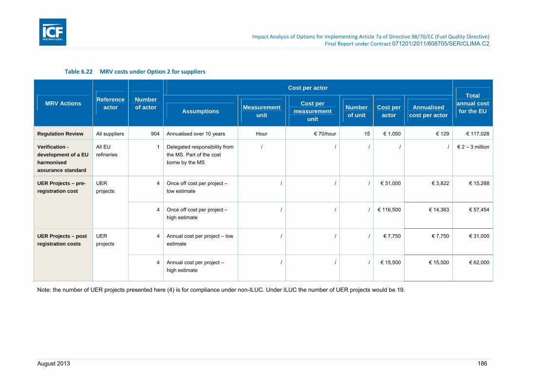
Impact Analysis of Options for Implementing Article 7a of Directive 98/70/EC (Fuel Quality Directive) Final Report under Contract 071201/2011/608705/SER/CLIMA.C2
August 2013 186
Table 6.22 MRV costs under Option 2 for suppliers
MRV Actions Reference
actor Number of actor
Cost per actor Total
annual cost for the EU Assumptions
Measurement unit
Cost per measurement
unit
Number of unit
Cost per actor
Annualised cost per actor
Regulation Review All suppliers 904 Annualised over 10 years Hour € 70/hour 15 € 1,050 € 129 € 117,028
Verification -
development of a EU
harmonised
assurance standard
All EU
refineries
1 Delegated responsibility from
the MS. Part of the cost
borne by the MS
/ / / / / € 2 – 3 million
UER Projects – pre-
registration cost
UER
projects
4 Once off cost per project –
low estimate
/ / / € 31,000 € 3,822 € 15,288
4 Once off cost per project –
high estimate
/ / / € 116,500 € 14,363 € 57,454
UER Projects – post
registration costs
UER
projects
4 Annual cost per project – low
estimate
/ / / € 7,750 € 7,750 € 31,000
4 Annual cost per project –
high estimate
/ / / € 15,500 € 15,500 € 62,000
Note: the number of UER projects presented here (4) is for compliance under non-ILUC. Under ILUC the number of UER projects would be 19.
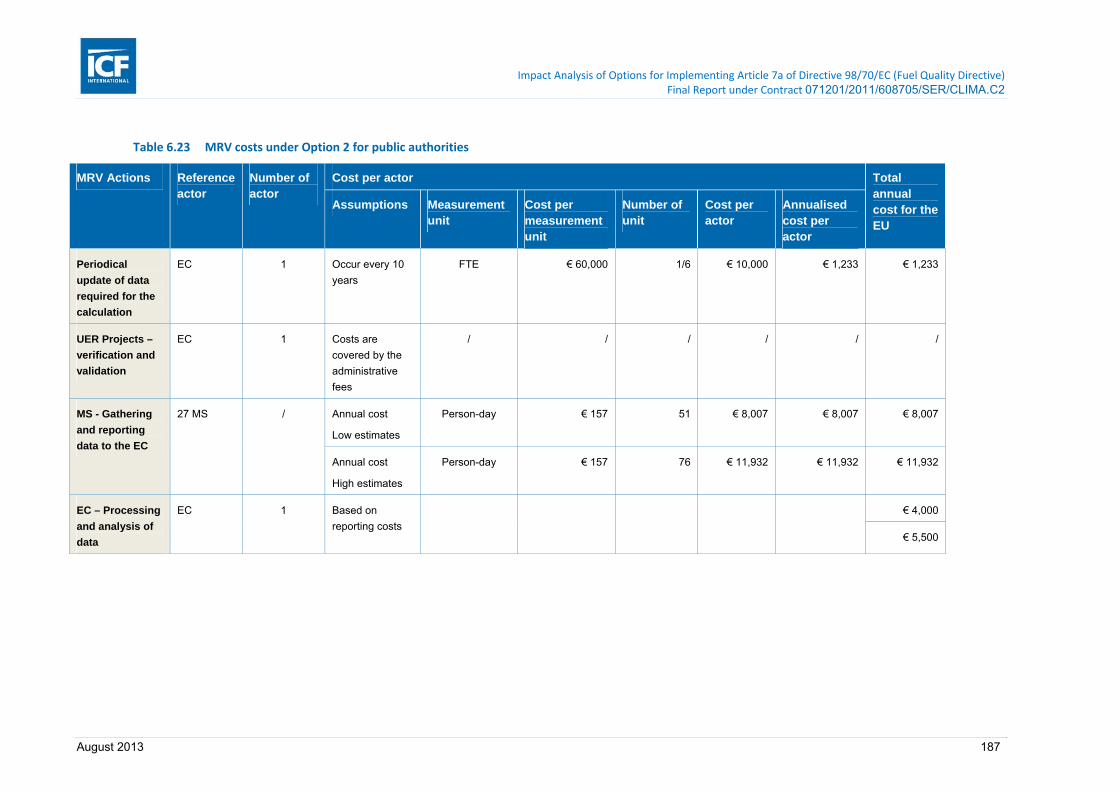
Impact Analysis of Options for Implementing Article 7a of Directive 98/70/EC (Fuel Quality Directive) Final Report under Contract 071201/2011/608705/SER/CLIMA.C2
August 2013 187
Table 6.23 MRV costs under Option 2 for public authorities
MRV Actions Reference actor
Number of actor
Cost per actor Total annual cost for the EU
Assumptions Measurement unit
Cost per measurement unit
Number of unit
Cost per actor
Annualised cost per actor
Periodical
update of data
required for the
calculation
EC 1 Occur every 10
years
FTE € 60,000 1/6 € 10,000 € 1,233 € 1,233
UER Projects –
verification and
validation
EC 1 Costs are
covered by the
administrative
fees
/ / / / / /
MS - Gathering
and reporting
data to the EC
27 MS / Annual cost
Low estimates
Person-day € 157 51 € 8,007 € 8,007 € 8,007
Annual cost
High estimates
Person-day € 157 76 € 11,932 € 11,932 € 11,932
EC – Processing
and analysis of
data
EC 1 Based on
reporting costs
€ 4,000
€ 5,500

Impact Analysis of Options for Implementing Article 7a of Directive 98/70/EC (Fuel Quality Directive) Final Report under Contract 071201/2011/608705/SER/CLIMA.C2
August 2013 188
Table 6.24 MRV costs under Option 3 for suppliers (incurred by both opted in and opted out suppliers)
MRV Actions Reference
actor Number of actor
Cost per actor Total annual cost for the EU
Assumptions Measurement
unit
Cost per measurement
unit
Number of unit
Cost per
actor
Annualised cost per actor
Regulation Review Refineries,
Suppliers,
Traders
904 Annualised over 10 years Hour € 70/hour 15 € 1,050 € 129 € 117,028
Verification -
development of a EU
harmonised assurance
standard
All EU
refineries
1 Delegated responsibility
from the MS. Part of the
cost borne by the MS
/ / / / / € 2 – 3
million
UER Projects – pre-
registration cost
UER projects 4 Once off cost per project –
low estimate
/ / / € 31,000 € 3,822 € 15,288
4 Once off cost per project –
high estimate
/ / / €
116,500
€ 14,363 € 57,454
UER Projects – post
registration costs
UER projects 4 Annual cost per project –
low estimate
/ / / € 7,750 € 7,750 € 31,000
4 Annual cost per project –
high estimate
/ / / € 15,500 € 15,500 € 62,000
Note: the number of UER projects presented here (4) is for compliance under non-ILUC. Under ILUC the number of UER projects would be 18.

Impact Analysis of Options for Implementing Article 7a of Directive 98/70/EC (Fuel Quality Directive) Final Report under Contract 071201/2011/608705/SER/CLIMA.C2
August 2013 189
Table 6.25 Additional MRV costs under Option 3 for opted out suppliers
MRV Actions Reference actor
Number of actors
Cost per actor Total annual cost for EU
(low)
Total annual cost for EU
(high) Assumptions Cost per
actor
Annualised cost per
actor(low)
Annualised cost per actor
(high)
LCA calculation – own
measurement
⅓ opting out
producers
19 Measured data for 2 stages
(extraction and refining)
€ 58,000 € 13,028 € 30,751 € 247,539 € 584,276
€ 100,950 € 22,676 € 53,523 € 430,846 € 1,016,943
LCA calculation –
engineering estimates
⅓ opting out
producers
19 Estimation - Engineering € 70,000 € 15,724 € 37,114 € 298,754 € 705,161
€ 93,000 € 20,890 € 49,308 € 396,916 € 936,856
LCA calculation – existing
model
⅓ opting out
producers
19 Estimation – Existing model
(e.g. GREET)
€ 11,500 € 2,583 € 6,097 € 49,081 € 115,848
€ 23,300 € 5,234 € 12,354 € 99,442 € 234,718
Verification and validation
cost
Opting out
refineries
56 External validation € 11,500 € 2,583 € 6,097 € 144,660 € 341,446
€ 23,300 € 5,234 € 12,354 € 293,093 € 691,800
Development of an internal
tool / spreadsheet
Simple
refineries
38 Annualised over 10 years € 2,800 -
€ 5,600
€ 345 € 690 € 13,118 € 26,236
Complex
refineries
18 Annualised over 10 years € 5,600 -
€ 11,200
€ 690 € 1381 € 12,428 € 24,855
Maintaining an internal tool
/ spreadsheet
Simple
refineries
38 Annual cost. Daily / weekly
activity
€ 18,200 € 18,200 € 18,200 € 691,600 € 691,600
Complex
refineries
18 Annual cost. Daily / weekly
activity
€ 36,400 € 36,400 € 36,400 € 655,200 € 655,200
Management and transfer
of data by fuel traders,
verification of this process
Opted out
traders
378 Administrative cost of fuel
traders is equal to 20% of costs
for EU and non-EU refineries
€ 6,770,308 € 13,926,273
Note: Low Estimates based on repeated calculations every 5 years and high estimates based on re-calculations every 2 years

Impact Analysis of Options for Implementing Article 7a of Directive 98/70/EC (Fuel Quality Directive) Final Report under Contract 071201/2011/608705/SER/CLIMA.C2
August 2013 190
Table 6.26 Additional MRV costs under Option 3 for opted in suppliers
MRV Actions Reference actor
Number of actor
Cost per actor Total annual
cost for the EU
Assumptions Measurement
unit
Cost per measurement
unit
Number of unit
Cost per actor
Annualised cost per
actor
Development of
internal tool / spread
sheet
Simple
refinery
49 Annualised over 10 years Hour € 70/hour 40 € 2,800 € 345 € 16,916
Hour € 70/hour 80 € 5,600 € 690 € 33,831
Complex
refinery
24 Annualised over 10 years Hour € 70/hour 80 € 5,600 € 690 € 16,570
Hour € 70/hour 160 € 11,200 € 1,381 € 33,141
Maintaining internal
tool / spread sheet
Simple
refinery
49 Annual cost
Daily / weekly activity
Hour € 70/hour 260 € 18,200 € 18,200 € 891,800
Complex
refinery
24 Annual cost
Daily / weekly activity
Hour € 70/hour 520 € 36,400 € 36,400 € 873,600
Internal and external
verification
Simple
refinery
49 Averaging cost of internal
and external auditing
Hour € 70/hour 15 € 1,050 € 1,050 € 51,450
Complex
refinery
24 Averaging cost of internal
and external auditing
Hour € 70/hour 30 € 2,100 € 2,100 € 50,400
Management and
transfer of data by fuel
traders and
verification of this
process
Opted in
traders
584 Administrative cost of fuel
traders is equivalent to 20%
of the costs for EU and
non-EU refineries
€4.7m
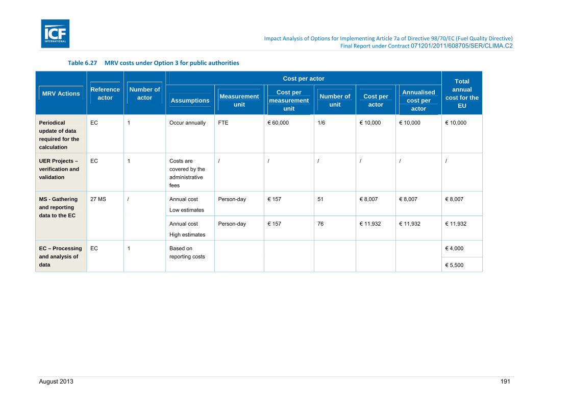
Impact Analysis of Options for Implementing Article 7a of Directive 98/70/EC (Fuel Quality Directive) Final Report under Contract 071201/2011/608705/SER/CLIMA.C2
August 2013 191
Table 6.27 MRV costs under Option 3 for public authorities
MRV Actions Reference
actor Number of
actor
Cost per actor Total annual
cost for the EU
Assumptions Measurement
unit
Cost per measurement
unit
Number of unit
Cost per actor
Annualised cost per
actor
Periodical
update of data
required for the
calculation
EC 1 Occur annually FTE € 60,000 1/6 € 10,000 € 10,000 € 10,000
UER Projects –
verification and
validation
EC 1 Costs are
covered by the
administrative
fees
/ / / / / /
MS - Gathering
and reporting
data to the EC
27 MS / Annual cost
Low estimates
Person-day € 157 51 € 8,007 € 8,007 € 8,007
Annual cost
High estimates
Person-day € 157 76 € 11,932 € 11,932 € 11,932
EC – Processing
and analysis of
data
EC 1 Based on
reporting costs
€ 4,000
€ 5,500

Impact Analysis of Options for Implementing Article 7a of Directive 98/70/EC (Fuel Quality Directive) Final Report under Contract 071201/2011/608705/SER/CLIMA.C2
August 2013 192
6.3 Results of the analysis of policy options
As described earlier, the choice of compliance for option 3, in terms of whether to opt in or to opt out, has been modelled by direct comparison of the modelled actual emissions intensity to the intensity under option 1. The selection of the minimum of these is what has been used as the determinant in this modelling of whether a supplier will opt in or opt out. In reality, if the additional costs of developing supplier specific data were taken into account, this would effectively decrease the number of suppliers opting out. The amount that this would decrease would be related to the potential compliance costs of implementing abatement measures since this would be the alternative that a supplier would need to undertake. This means that the modelling may overestimate the number of suppliers that opt out, which will lead to an underestimate of the environmental impact and an underestimate of the compliance cost.
6.3.1 Environmental impacts
The environmental impacts of the FQD are related to the 6% reduction target from the 2010 base year intensity. The relative environmental impacts of the different policy options to calculate the intensities are related to how, in aggregate, each supplier’s total intensity as calculated exceeds the target intensity of 83.002 g/MJ, including the negative contributions to this total by suppliers that already meet and surpass the target (full joint reporting). The sum across the suppliers of the reductions needed to meet the FQD target from the baseline (i.e., EU average distance to target) for each of the policy options is included in the table below.
Table 6.28 Estimated emission reductions from the baseline to meet the target of 83.002 (Mt CO2e)
Sensitivity Scenario No joint reporting
(Mt CO2)
Full joint reporting (Mt CO
2)
Non-ILUC Option 0 10.45 10.32
Option 1 10.81 10.32
Option 2 10.81 10.32
Option 3 10.33 9.84
Option 5 10.82 10.32
ILUC Option 0 48.08 48.08
Option 1 48.08 48.08
Option 2 48.08 48.08
Option 3 47.54 47.54
Option 5 48.08 48.08
Note: See Section 6.3.1.2 for interpretation of the emissions reductions under Option 3.
The table above, and as outlined in the Task 1.3 work86, identifies that, when considering full joint reporting, under business as usual and based on the fuel projections of the baseline the
86 Note that the task 1.3 results of the assessment of what measures excluding switching options would deliver compliance with the target assuming a reduction to target based on the original default intensities. The analysis in

Impact Analysis of Options for Implementing Article 7a of Directive 98/70/EC (Fuel Quality Directive) Final Report under Contract 071201/2011/608705/SER/CLIMA.C2
August 2013 193
FQD reduction target will not be met as a matter of course, and that reductions will be needed to meet the target. What was unknown from this analysis was whether, when analysed at a granular supplier level if the aggregate impacts would differ from this figure substantially. The results of no joint reporting column in the table above suggest that the aggregate impacts if there is no joint reporting will not differ substantially from the otherwise calculated impacts assuming full joint reporting.
6.3.1.2 Environmental Impacts under Option 3
Option 3 leads to a reduced EU average distance to target. This is a consequence of the definition of option 3 in which suppliers have the choice to opt in or opt out, and those that opt in may effectively be ‘under reporting’ their emissions: i.e. reported emissions would be lower than actual emissions.
Box 7 shows a hypothetical and simplified scenario of a selection of suppliers and their actual intensities represented as blue circles, and shows an indication of which suppliers would opt out and which suppliers would opt in. It is a simplification because only one default value is shown, and it is hypothetical in terms of the market distribution of suppliers.
Box 7 Hypothetical and simplified plot of suppliers and reporting under option 3
In the 1st iteration of option 3, the default value (the green vertical line in the figure above) represents the average intensity of the entire supplier market volume. In the 2nd iteration of option 3, i.e. after adjustment of the default value, the default value (the brown vertical line in the figure above) would represent the average intensity of those suppliers which opted in during the 1st iteration.
The distance to target when calculated from the reported intensities (green crosses in Box 7) during the 1st iteration will be less than if the distances to target had been calculated from actual intensities (blue circles in Box 7) i.e. per option 5. During the 2nd iteration after the default value(s) were updated, then the updated default value would more accurately
this task has assumed revised default unit intensities as described in section 6.2.3, which leads to higher reductions needed to reach the target.

Impact Analysis of Options for Implementing Article 7a of Directive 98/70/EC (Fuel Quality Directive) Final Report under Contract 071201/2011/608705/SER/CLIMA.C2
August 2013 194
represent intensities of the suppliers that opted in during the first iteration. However, at the 2nd iteration, a different selection of suppliers would then be expected to opt out and in.
This analysis assumes that suppliers would opt out if their actual emissions are below the default value and suppliers would opt in if their actual emissions are above the default value. As discussed earlier in section 5.2.7 this opting decision would also be influenced by the administrative costs of reporting actual emissions. If those administrative costs were taken into account, depending on the relative costs of compliance versus administration, this would act to discourage some suppliers from opting out.
Due to the definition of option 3 and the choice available to suppliers, the option leads to a reduced distance to target, which is effectively the same as suggesting that its environmental effectiveness is lower than that of the policy options that do not give suppliers a choice (options 0, 1, 2 and 5). Associated with the lower emission reductions are also lower compliance and administrative costs compared to e.g. option 5. This is important to consider when comparing the policy options that, for example, the higher costs associated with option 1 compared to option 3 are as a result of achieving higher emission reductions.
A fairer comparison of the options, i.e. a comparison that took account of the different emission reductions, would indicate that the comparable costs (compliance and administrative) of option 3 would lie in the range between those of option 1 and option 5.
6.3.1.3 Results
The results of the analysis that has been undertaken for the non-ILUC and ILUC scenarios are presented in absolute figures for each of the policy options in Table 6.30, which assume full joint reporting given the negligible difference in comparison to the "no joint reporting" values. The relative impacts of each policy option compared to option 0 are shown in Error! Reference source not found.. These tables also include nominal results for policy option 5, which has been additionally requested by the Commission. .
The results show that there is very little variation among the options in terms of environmental impacts. As explained above, Option 3 leads to a reduced distance to target and so can have lower compliance costs. The number of suppliers estimated to opt in / out is shown below in the table.
Table 6.29 Opted in and opted out suppliers under Option 3
Option 3 Producers Traders
Number of opted in suppliers 51 397 (non-ILUC)383 (ILUC)
Number of opted out suppliers 39 378 (non-ILUC)392 (ILUC)

Impact Analysis of Options for Implementing Article 7a of Directive 98/70/EC (Fuel Quality Directive) Final Report under Contract 071201/2011/608705/SER/CLIMA.C2
August 2013 195
Table 6.30 Summary results of the energy, GHG emissions and intensity of each policy option together with the absolute compliance costs to reach the target and the absolute administrative costs
Absolute costs non‐ILUC ILUC
Option 0 Option 1 Option 2 Option 3 Option 5 Option 0 Option 1 Option 2 Option 3 Option 5
Transport energy demand PJ 10,879 10,879 10,879 10,880 10,879 10,837 10,839 10,837 10,840 10,840
GHG emissions Mt CO2e 903 902 903 903 902 899 898 899 898 898
Final intensity (full joint reporting) g/MJ 83.0 82.9 83.0 83.0 82.9 83.0 82.8 83.0 82.8 82.8
Compliance costs biofuels €m ‐6 ‐6 ‐6 ‐13 ‐6 406 351 406 351 351 UERs €m
12 12 12 12 12 1211 1167 1211 1167 1167 crude switching €m
0 1 0 0 1 0 32 0 37 44 product switching
€m 0 2 0 1 2 0 17 0 15 21
total €m 6 8 6 1 9 1618 1567 1618 1571 1584
Administrative costs
low €m 2 15 2 18 21 2 15 2 18 21 average €m
3 15 3 23 31 3 16 3 23 32 high €m
3 16 3 28 42 4 16 4 29 42
Total costs €m 9 24 9 24 40 1621 1583 1621 1594 1615
Note: A more appropriate comparison of costs reflecting the lower environmental effectiveness of Option 3 would be to assume that compliance and administrative costs for this option lie in the
range between those for option 1 and option 5, as per discussion in Section 6.3.1.2.

Impact Analysis of Options for Implementing Article 7a of Directive 98/70/EC (Fuel Quality Directive) Final Report under Contract 071201/2011/608705/SER/CLIMA.C2
August 2013 196
Table 6.31 Summary results of the energy, GHG emissions and intensity of each policy option together with the compliance costs to reach the target and the administrative costs, as compared to Option 0
Absolute costs non‐ILUC ILUC
Option 0 Option 1 Option 2 Option 3 Option 5 Option 0 Option 1 Option 2 Option 3 Option 5
Transport energy demand PJ 0 0 0 1 0 0 2 0 3 3
GHG emissions Mt CO2e 0 ‐1 0 0 ‐1 0 ‐1 0 ‐1 ‐1
Final intensity (full joint reporting) g/MJ 0.0 ‐0.1 0.0 0.0 ‐0.1 0.0 ‐0.1 0.0 ‐0.1 ‐0.1
Compliance costs biofuels €m 0 0 0 ‐7 0 0 ‐55 0 ‐55 ‐55
UERs €m 0 0 0 0 0 0 ‐44 0 ‐44 ‐44
crude switching €m 0 1 0 0 1 0 32 0 37 44
product switching €m 0 2 0 1 2 0 17 0 15 21
total €m 0 2 0 ‐5 3 0 ‐51 0 ‐47 ‐34
Administrative costs low €m 0 12 0 15 19 0 12 0 16 29
average €m 0 13 0 20 29 0 13 0 20 29
high €m 0 13 0 25 38 0 13 0 25 38
Total costs €m 0 15 0 15 31 0 ‐38 0 ‐26 ‐5
Note: A more appropriate comparison of costs reflecting the lower environmental effectiveness of Option 3 would be to assume that compliance and administrative costs for this option lie in the
range between those for option 1 and option 5, as per discussion in Section 6.3.1.2.

Impact Analysis of Options for Implementing Article 7a of Directive 98/70/EC (Fuel Quality Directive) Final Report under Contract 071201/2011/608705/SER/CLIMA.C2
August 2013 197
Option 3 is the policy option which provides suppliers with the option to opt out of using the default unit GHG intensities and hence use their supplier specific intensities instead. Suppliers have been modelled as only taking up this option if their intensity is lower by taking up this option. Therefore, the total emissions reductions to be made under Option 3 are lower than under Options 1 and 2. However the distance over the target is only slightly less than for the other options. This result can be explained by looking at the distribution of the suppliers intensities with high granular detail. Figure 6.8 shows this granular detail by plotting suppliers in order of their estimated total intensity against their cumulative normalised total supply volumes under each of policy options 1, 2 and 3. The figure shows that for the non-ILUC scenario less than 10% of suppliers by volumes supplied are estimated to be under the target under BAU, and under the ILUC scenario no suppliers are modelled under the 83g/MJ target. Hence, as modelled, there is very little quantity below the target which could effectively ‘offset’ suppliers above the target when assuming full joint reporting.
Furthermore on option 3, the small reduction in the emissions distance from target is partly a reflection of the lag in the updating of the default intensities for the opt in suppliers (lag as described in section 5.2.7 of the Task 2-1 report). If there was no ‘lag’ in this updating process, then the total emissions distance from target of option 3 would be equal to that for the other options, because the reduction in reported emissions from the opted out suppliers would be exactly compensated by the appropriate increase in the default intensities for the opt in suppliers. However because of the lag in the system, there would be expected to be a difference between the distance to target for option 3 compared to options 0/1/2 as the suppliers in 2020 would be opting in or opting out from a set of default unit GHG intensities that were updated in a previous year (2019 or before).
Figure 6.8 Suppliers estimated total intensity (ordered lowest to highest) as a function of cumulative normalised total supply volumes under each policy option and compared to the target (source: this work)
Non-ILUC ILUC
In terms of the potential for suppliers to take up abatement options associated with switching feedstocks or products, Table 6.32 below summarises the potential for uptake of switching compliance options for policy options 1 and 3 opt in.

Impact Analysis of Options for Implementing Article 7a of Directive 98/70/EC (Fuel Quality Directive) Final Report under Contract 071201/2011/608705/SER/CLIMA.C2
August 2013 198
Table 6.32 Emission reduction potential for crude and product switching for options 1 and 3 opt in
Sensitivity Scenario
Abatement potential (Mt CO2) from switching feedstock categories to conventional
Abatement potential (Mt CO2) from switching product imports to conventional
From natural bitumen
From oil shale
From CTL
From GTL
From natural bitumen
Non-ILUC Option 1 4.6 0.1 1.5 0.5 0.4
Option 3 opt
in
0 0.1 1.5 0.5 0.4
ILUC Option 1 4.6 0.3 1.6 0.5 0.4
Option 3 opt
in
0 0.1 1.6 0.5 0.4
The table above shows that, if the crude and product switching measures are more cost effective than other compliance measures, these measures alone may have the potential to achieve a large proportion of the emissions reductions required by suppliers to meet the target under options 1 and 3 (these switching options are not available under Options 0 and 2). As will be shown in Task 3, the crude and product switching forms only a small part of the compliance as the biofuel and UER options have been estimated to be more cost effective.
Under the ILUC sensitivity, the potential reductions from crude and product switching will not form a large proportion of the distance to target (even if these measures are cost effective), which will result in larger uptake of biofuels and/ or UERs.
6.3.1.4 Limitations
Three main limitations of this analysis should be highlighted:
■ The flat proportioning of biofuels, electricity, CNG, and hydrogen across the suppliers. These would likely in reality be not evenly distributed among suppliers and so with their variation they may well lead to increased diversity among suppliers’ total greenhouse gas intensities and which would lead to some suppliers’ intensities increasing the overall distance to target.
■ The assumed true emissions intensities could form a narrower range that suppliers’ actual intensities. . This is not considered to be however a major limitation of the modelling of Option 387, because only those suppliers that opt out would utilise the supplier-specific method such that even if a more diverse dataset of pathways with some higher intensity crudes were utilised, the analysis would assume that such suppliers would opt in and use the default unit GHG intensities. If suppliers’ actual intensities were lower than those assumed, then Option 3 as modelled would overestimate the reduction to target and hence cost impacts.
■ MS level overall impacts are the same due to the overall mathematical equivalence in aggregate of the unit GHG intensity calculations. In reality, Member States may develop their unit intensities differently resulting in additional variation among the Member States and hence among the suppliers.
Although not a limitation per se, it is worth noting that the analysis for Option 3 is representative for its first year(s) of operation before adjustment of the default intensities for the opted in suppliers. The environmental impacts after this point would shift.
87 It would be a limitation if Option 5 were to be modelled for example though.

Impact Analysis of Options for Implementing Article 7a of Directive 98/70/EC (Fuel Quality Directive) Final Report under Contract 071201/2011/608705/SER/CLIMA.C2
August 2013 199
6.3.2 Administrative impacts
The total administrative costs were included in Table 6.30 and Table 6.31 above. This section presents the results of the administrative impacts in greater detail.
There are small differences between the administrative impacts under the non-ILUC and ILUC scenarios due to the different numbers of UER projects that have been estimated to be necessary as part of compliance. The number of UER projects has an impact on the administrative costs due to the pre-registration and post-registration costs per UER project (and hence the administrative costs in Table 6.31 which assumes no UER projects).
Estimates have also been made for policy option 5. These estimates have been made by assuming the same costs for option 3 but assuming that all suppliers opt out and none opt in.
Table 6.33 summarises the results for the central (non-ILUC) case. Table 6.34 shows the very slightly higher results for the ILUC sensitivity. The results suggest that from an administrative cost perspective, there is no marginal difference of option 2 over option 0. Options 1, 3 and 5 have higher administrative costs than option 0. The administrative cost estimates for the policy options with supplier specific requirements are higher than the estimates for Option 1, reflecting the increased burdens on opting out suppliers, and have a wider range than those for option 1, which reflects the increased uncertainty in the administrative cost estimates for supplier-specific reporting.
Table 6.33 Total estimated administrative costs (€m / yr) per policy option under non‐ILUC
Scenario Subtotals
Supplier cost (€m/yr)
Authority cost (€m/yr)
Total cost (€m/yr)
Difference from option 0 (€m/yr)
Low High Low High Low High Low High
Option 0 Total 2.2 3.2 0.01 0.02 2.2 3.3 - -
Option 1 Total 14.6 15.9 0.01 0.02 14.6 15.9 12.5 12.7
Option 2 Total 2.2 3.2 0.01 0.02 2.2 3.3 0.0 0.0
Option 3 All 2.2 3.2 0.02 0.03 2.2 3.3 - -
Additionally
for opt in 6.6 6.7 6.6 6.7 - -
Additionally
for opt out 8.9 18.2 8.9 18.2 - -
Total 17.6 28.1 0.02 0.03 17.6 28.2 15.5 24.9
Option 5 Total 20.9 41.6 0.02 0.03 20.9 41.6 18.7 38.3
Note: A more appropriate comparison of costs reflecting the lower environmental effectiveness of Option 3 would be to assume
that administrative costs for this option lie in the range between those for option 1 and option 5, as per discussion in Section
6.3.1.2.

Impact Analysis of Options for Implementing Article 7a of Directive 98/70/EC (Fuel Quality Directive) Final Report under Contract 071201/2011/608705/SER/CLIMA.C2
August 2013 200
Table 6.34 Total estimated administrative costs (€m / yr) per policy option under ILUC sensitivity
Scenario Subtotals
Supplier cost (€m/yr)
Authority cost (€m/yr)
Total cost (€m/yr)
Difference from option 0 (€m/yr)
Low High Low High Low High Low High
Option 0 Total 2.3 3.7 0.01 0.02 2.4 3.7 - -
Option 1 Total 14.8 16.3 0.01 0.02 14.8 16.4 12.5 12.7
Option 2 Total 2.3 3.7 0.01 0.02 2.4 3.7 0.0 0.0
Option 3 All 2.3 3.7 0.02 0.03 2.3 3.7 - -
Additionally
for opt in 6.4 6.5 6.4 6.5 - -
Additionally
for opt out 8.9 17.5 8.9 17.5 - -
Total 17.6 27.7 0.02 0.03 17.6 27.7 15.3 24.0
Option 5 Total 21.1 42.0 0.02 0.03 21.1 42.0 18.7 38.3
Note: A more appropriate comparison of costs reflecting the lower environmental effectiveness of Option 3 would be to assume
that administrative costs for this option lie in the range between those for option 1 and option 5, as per discussion in Section
6.3.1.2.
The estimated annual absolute administrative costs presented above have been recalculated on the basis of litres of product supplied. These estimates in Eurocents per 100 litres are shown in Table 6.35 (non ILUC) and Table 6.36 (ILUC) below.

Impact Analysis of Options for Implementing Article 7a of Directive 98/70/EC (Fuel Quality Directive) Final Report under Contract 071201/2011/608705/SER/CLIMA.C2
August 2013 201
Table 6.35 Total estimated administrative costs (€cents / 100 litres of product) per policy option under non‐ILUC
Scenario Subtotals
Supplier cost (€ct / 100litres )
Authority cost (€ct / 100 litres )
Total cost (€ct / 100 litres )
Difference from option 0 (€ct /
100 litres )
Low High Low High Low High Low High
Option 0 Total 0.07 0.10 0.0004 0.0006 0.07 0.10
Option 1 Total 0.45 0.49 0.0004 0.0006 0.45 0.49 0.39 0.39
Option 2 Total 0.07 0.10 0.0004 0.0006 0.07 0.10 0.00 0.00
Option 3 All 0.07 0.10 0.0007 0.0009 0.07 0.10
Additionally
for opt in 0.20 0.21 0 0 0.20 0.21
Additionally
for opt out 0.28 0.56 0 0 0.27 0.53
Total 0.55 0.87 0.0007 0.0009 0.55 0.87 0.48 0.77
Option 5 Total 0.65 1.29 0.0007 0.0009 0.65 1.29 0.58 1.19
Note: A more appropriate comparison of costs reflecting the lower environmental effectiveness of Option 3 would be to assume
that compliance and administrative costs for this option lie in the range between those for option 1 and option 5, as per
discussion in Section 6.3.1.2.
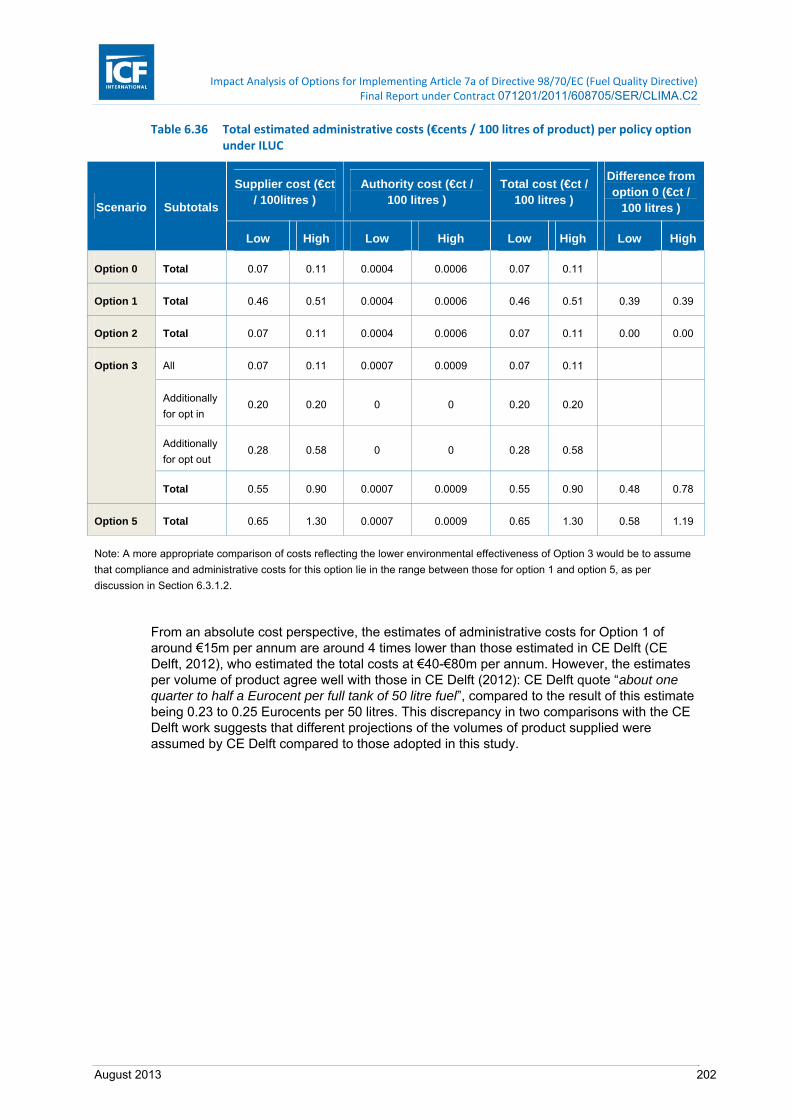
Impact Analysis of Options for Implementing Article 7a of Directive 98/70/EC (Fuel Quality Directive) Final Report under Contract 071201/2011/608705/SER/CLIMA.C2
August 2013 202
Table 6.36 Total estimated administrative costs (€cents / 100 litres of product) per policy option under ILUC
Scenario Subtotals
Supplier cost (€ct / 100litres )
Authority cost (€ct / 100 litres )
Total cost (€ct / 100 litres )
Difference from option 0 (€ct /
100 litres )
Low High Low High Low High Low High
Option 0 Total 0.07 0.11 0.0004 0.0006 0.07 0.11
Option 1 Total 0.46 0.51 0.0004 0.0006 0.46 0.51 0.39 0.39
Option 2 Total 0.07 0.11 0.0004 0.0006 0.07 0.11 0.00 0.00
Option 3 All 0.07 0.11 0.0007 0.0009 0.07 0.11
Additionally
for opt in 0.20 0.20 0 0 0.20 0.20
Additionally
for opt out 0.28 0.58 0 0 0.28 0.58
Total 0.55 0.90 0.0007 0.0009 0.55 0.90 0.48 0.78
Option 5 Total 0.65 1.30 0.0007 0.0009 0.65 1.30 0.58 1.19
Note: A more appropriate comparison of costs reflecting the lower environmental effectiveness of Option 3 would be to assume
that compliance and administrative costs for this option lie in the range between those for option 1 and option 5, as per
discussion in Section 6.3.1.2.
From an absolute cost perspective, the estimates of administrative costs for Option 1 of around €15m per annum are around 4 times lower than those estimated in CE Delft (CE Delft, 2012), who estimated the total costs at €40-€80m per annum. However, the estimates per volume of product agree well with those in CE Delft (2012): CE Delft quote “about one quarter to half a Eurocent per full tank of 50 litre fuel”, compared to the result of this estimate being 0.23 to 0.25 Eurocents per 50 litres. This discrepancy in two comparisons with the CE Delft work suggests that different projections of the volumes of product supplied were assumed by CE Delft compared to those adopted in this study.
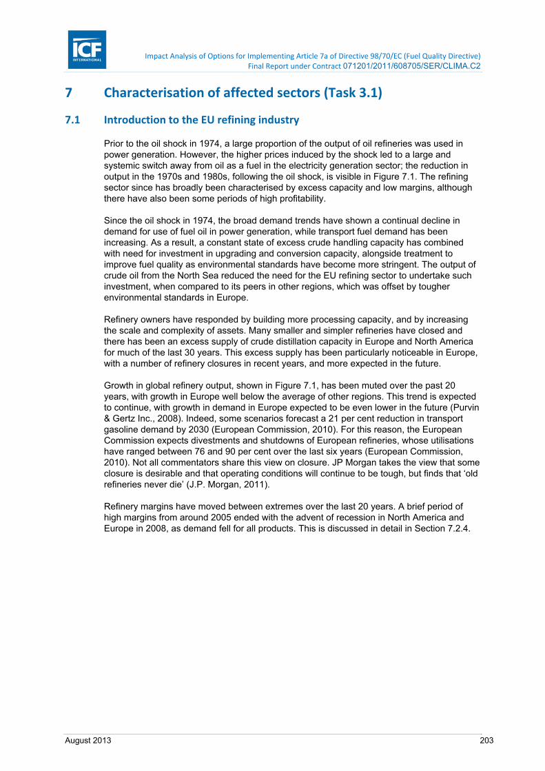
Impact Analysis of Options for Implementing Article 7a of Directive 98/70/EC (Fuel Quality Directive) Final Report under Contract 071201/2011/608705/SER/CLIMA.C2
August 2013 203
7 Characterisation of affected sectors (Task 3.1)
7.1 Introduction to the EU refining industry
Prior to the oil shock in 1974, a large proportion of the output of oil refineries was used in power generation. However, the higher prices induced by the shock led to a large and systemic switch away from oil as a fuel in the electricity generation sector; the reduction in output in the 1970s and 1980s, following the oil shock, is visible in Figure 7.1. The refining sector since has broadly been characterised by excess capacity and low margins, although there have also been some periods of high profitability.
Since the oil shock in 1974, the broad demand trends have shown a continual decline in demand for use of fuel oil in power generation, while transport fuel demand has been increasing. As a result, a constant state of excess crude handling capacity has combined with need for investment in upgrading and conversion capacity, alongside treatment to improve fuel quality as environmental standards have become more stringent. The output of crude oil from the North Sea reduced the need for the EU refining sector to undertake such investment, when compared to its peers in other regions, which was offset by tougher environmental standards in Europe.
Refinery owners have responded by building more processing capacity, and by increasing the scale and complexity of assets. Many smaller and simpler refineries have closed and there has been an excess supply of crude distillation capacity in Europe and North America for much of the last 30 years. This excess supply has been particularly noticeable in Europe, with a number of refinery closures in recent years, and more expected in the future.
Growth in global refinery output, shown in Figure 7.1, has been muted over the past 20 years, with growth in Europe well below the average of other regions. This trend is expected to continue, with growth in demand in Europe expected to be even lower in the future (Purvin & Gertz Inc., 2008). Indeed, some scenarios forecast a 21 per cent reduction in transport gasoline demand by 2030 (European Commission, 2010). For this reason, the European Commission expects divestments and shutdowns of European refineries, whose utilisations have ranged between 76 and 90 per cent over the last six years (European Commission, 2010). Not all commentators share this view on closure. JP Morgan takes the view that some closure is desirable and that operating conditions will continue to be tough, but finds that ‘old refineries never die’ (J.P. Morgan, 2011).
Refinery margins have moved between extremes over the last 20 years. A brief period of high margins from around 2005 ended with the advent of recession in North America and Europe in 2008, as demand fell for all products. This is discussed in detail in Section 7.2.4.
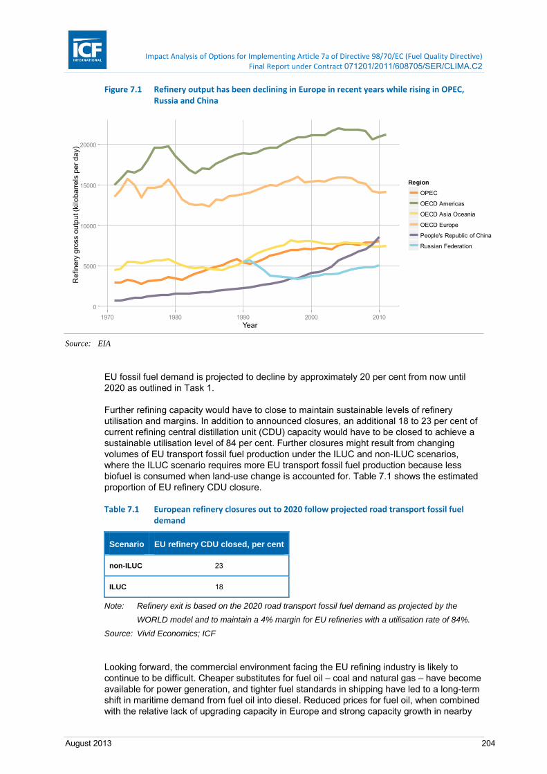
Impact Analysis of Options for Implementing Article 7a of Directive 98/70/EC (Fuel Quality Directive) Final Report under Contract 071201/2011/608705/SER/CLIMA.C2
August 2013 204
Figure 7.1 Refinery output has been declining in Europe in recent years while rising in OPEC, Russia and China
Source: EIA
EU fossil fuel demand is projected to decline by approximately 20 per cent from now until 2020 as outlined in Task 1.
Further refining capacity would have to close to maintain sustainable levels of refinery utilisation and margins. In addition to announced closures, an additional 18 to 23 per cent of current refining central distillation unit (CDU) capacity would have to be closed to achieve a sustainable utilisation level of 84 per cent. Further closures might result from changing volumes of EU transport fossil fuel production under the ILUC and non-ILUC scenarios, where the ILUC scenario requires more EU transport fossil fuel production because less biofuel is consumed when land-use change is accounted for. Table 7.1 shows the estimated proportion of EU refinery CDU closure.
Table 7.1 European refinery closures out to 2020 follow projected road transport fossil fuel demand
Scenario EU refinery CDU closed, per cent
non-ILUC 23
ILUC 18
Note: Refinery exit is based on the 2020 road transport fossil fuel demand as projected by the
WORLD model and to maintain a 4% margin for EU refineries with a utilisation rate of 84%.
Source: Vivid Economics; ICF
Looking forward, the commercial environment facing the EU refining industry is likely to continue to be difficult. Cheaper substitutes for fuel oil – coal and natural gas – have become available for power generation, and tighter fuel standards in shipping have led to a long-term shift in maritime demand from fuel oil into diesel. Reduced prices for fuel oil, when combined with the relative lack of upgrading capacity in Europe and strong capacity growth in nearby
0
5000
10000
15000
20000
1970 1980 1990 2000 2010Year
Re
fine
ry g
ross
ou
tpu
t (ki
lob
arr
els
pe
r d
ay)
Region
OPEC
OECD Americas
OECD Asia Oceania
OECD Europe
People's Republic of China
Russian Federation

Impact Analysis of Options for Implementing Article 7a of Directive 98/70/EC (Fuel Quality Directive) Final Report under Contract 071201/2011/608705/SER/CLIMA.C2
August 2013 205
markets, such as the Middle East, means that refining margins are likely to be, on average, low in future years. Further, saturated personal mobility markets coupled with improving vehicle efficiency have led to structurally-declining demand; a new feature of land transport fuel markets after a century of growth. The declining demand has been dictated by increased use of biofuels, mandatory standards for improved vehicle fuel efficiency and in the future the possible partial electrification of the vehicle fleet. Further pressure on margins originates from higher costs of energy in the form of CO2 pricing via the emissions trading scheme, and perhaps in the future the presence of mandatory regulations for refinery energy management including the cogeneration of heat and power as well as the capture and storage of CO2 emissions.
7.2 Structure of downstream industry
The structure of the industry modifies the impact of Fuel Quality Directive options
7.2.1 Location and key statistics of the EU refining industry
One can define the EU refining industry as all refineries in the Oil and Gas Journal’s database, except for eleven facilities which are excluded because they are not integrated into the transport fuel sector; for example, because they are primarily asphalt plants. As shown in Figure 7.2, the EU refining industry accounts for around 17 per cent of global refining capacity (Europia, 2011a)). The turnover of the EU27 industry sector known as ‘coke and refined petroleum products’ was €419 billion, in 2008, the latest year for which consistent EU-wide data is available (Eurostat, 2012). Gross value added in recent years has been around €30 billion each year and employment has been around 190,000 people. Labour productivity, measured as gross value added for each employee, was €160,000 in 2010; this is higher than the economy wide average due, among other things, to the high capital intensity of the industry, see Figure 7.4.
Figure 7.2 The bulk of global refining capacity is found in North America and the Asia‐Pacific, though European countries also contribute a substantial share
Source: ENI
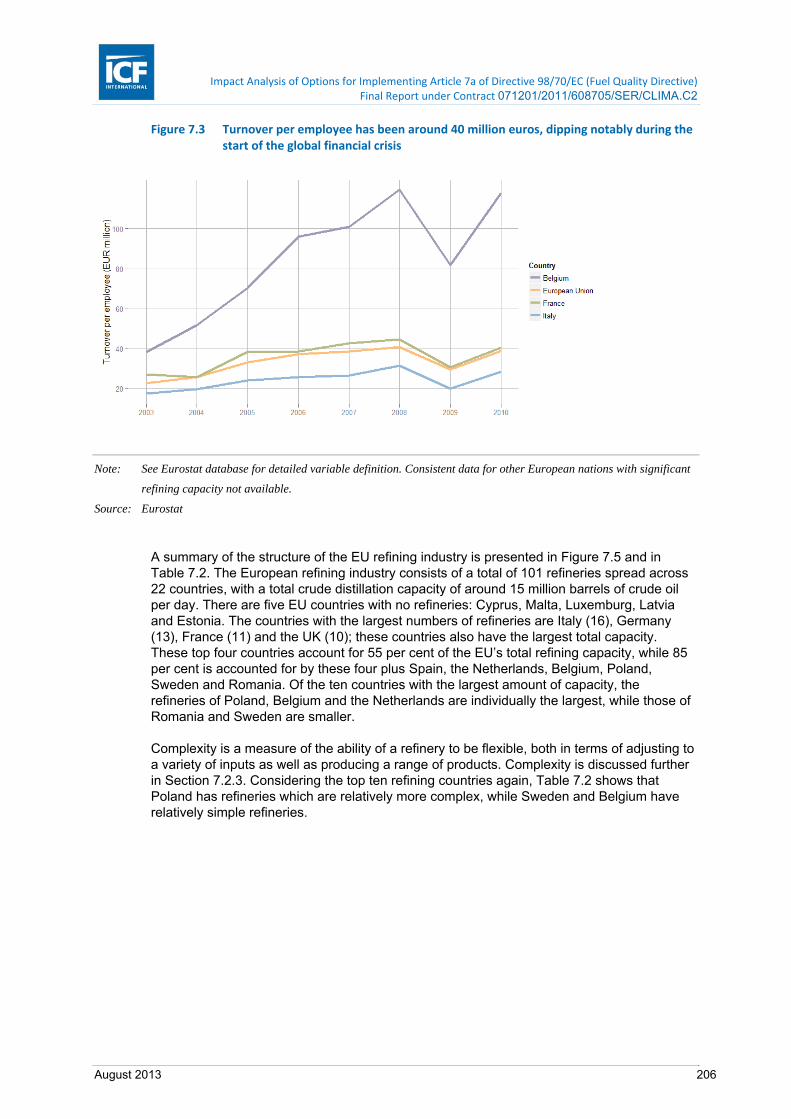
Impact Analysis of Options for Implementing Article 7a of Directive 98/70/EC (Fuel Quality Directive) Final Report under Contract 071201/2011/608705/SER/CLIMA.C2
August 2013 206
Figure 7.3 Turnover per employee has been around 40 million euros, dipping notably during the start of the global financial crisis
Note: See Eurostat database for detailed variable definition. Consistent data for other European nations with significant
refining capacity not available.
Source: Eurostat
A summary of the structure of the EU refining industry is presented in Figure 7.5 and in Table 7.2. The European refining industry consists of a total of 101 refineries spread across 22 countries, with a total crude distillation capacity of around 15 million barrels of crude oil per day. There are five EU countries with no refineries: Cyprus, Malta, Luxemburg, Latvia and Estonia. The countries with the largest numbers of refineries are Italy (16), Germany (13), France (11) and the UK (10); these countries also have the largest total capacity. These top four countries account for 55 per cent of the EU’s total refining capacity, while 85 per cent is accounted for by these four plus Spain, the Netherlands, Belgium, Poland, Sweden and Romania. Of the ten countries with the largest amount of capacity, the refineries of Poland, Belgium and the Netherlands are individually the largest, while those of Romania and Sweden are smaller.
Complexity is a measure of the ability of a refinery to be flexible, both in terms of adjusting to a variety of inputs as well as producing a range of products. Complexity is discussed further in Section 7.2.3. Considering the top ten refining countries again, Table 7.2 shows that Poland has refineries which are relatively more complex, while Sweden and Belgium have relatively simple refineries.

Impact Analysis of Options for Implementing Article 7a of Directive 98/70/EC (Fuel Quality Directive) Final Report under Contract 071201/2011/608705/SER/CLIMA.C2
August 2013 207
Figure 7.4 Labour productivity in the coke and refined petroleum sector under €200,000 in 2010, down by approximately one‐third since 2005
Note: See Eurostat database for detailed variable definition. Consistent data for other European nations with significant
refining capacity not available.
Source: Vivid Economics from Eurostat data
Figure 7.5 shows the distribution of refineries in the EU as well as the key characteristics of complexity and size. A large share of capacity is concentrated around the Rotterdam oil trading hub, including Shell’s 404,000 barrels-per-day refinery at Pernis in the Netherlands: the largest in the EU. With a couple of exceptions in central Poland and southern Germany, all of the largest refineries are located near the coast, where access to raw materials and export markets is less costly. Many inland refineries, such as those in Romania, are smaller and associated with local sources of crude or specialised demand. Coastal refineries are generally better positioned to alter their crude mix, say in response to the Fuel Quality Directive, as they have less costly access to seaborne trade in crude of various types; inland refineries will typically be restricted to crude either produced locally or available via pipeline and so will face any exposure to altered costs without the same scope to alter their crude diet.
Table 7.2 Over fifty per cent of the EU’s refining capacity is in Germany, Italy, the UK and France
Country Average CDU capacity
(b/cd)
Average complexity
(index) Number of refineries
Total CDU capacity in
country (kb/cd)
Austria 208,600 6.5 1 209
Belgium 239,607 6.0 3 719
Bulgaria 115,240 6.1 1 115
Czech Republic 61,000 6.5 3 183
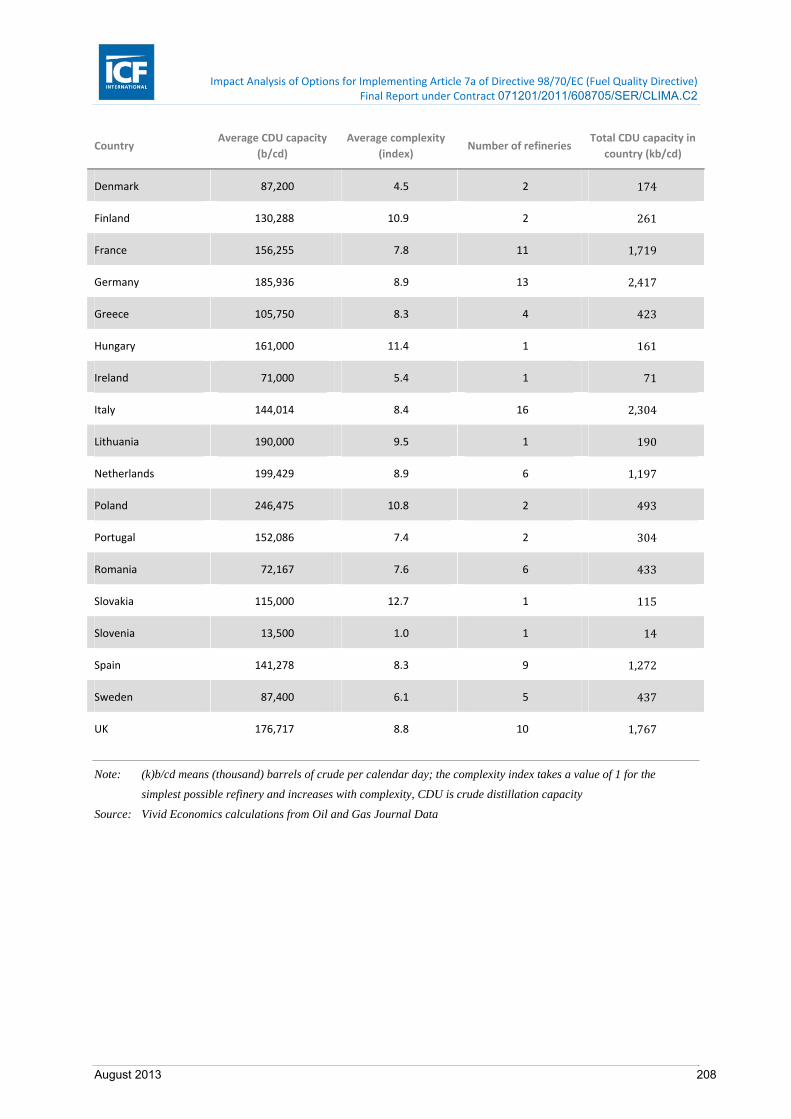
Impact Analysis of Options for Implementing Article 7a of Directive 98/70/EC (Fuel Quality Directive) Final Report under Contract 071201/2011/608705/SER/CLIMA.C2
August 2013 208
Country Average CDU capacity
(b/cd)
Average complexity
(index) Number of refineries
Total CDU capacity in
country (kb/cd)
Denmark 87,200 4.5 2 174
Finland 130,288 10.9 2 261
France 156,255 7.8 11 1,719
Germany 185,936 8.9 13 2,417
Greece 105,750 8.3 4 423
Hungary 161,000 11.4 1 161
Ireland 71,000 5.4 1 71
Italy 144,014 8.4 16 2,304
Lithuania 190,000 9.5 1 190
Netherlands 199,429 8.9 6 1,197
Poland 246,475 10.8 2 493
Portugal 152,086 7.4 2 304
Romania 72,167 7.6 6 433
Slovakia 115,000 12.7 1 115
Slovenia 13,500 1.0 1 14
Spain 141,278 8.3 9 1,272
Sweden 87,400 6.1 5 437
UK 176,717 8.8 10 1,767
Note: (k)b/cd means (thousand) barrels of crude per calendar day; the complexity index takes a value of 1 for the
simplest possible refinery and increases with complexity, CDU is crude distillation capacity
Source: Vivid Economics calculations from Oil and Gas Journal Data
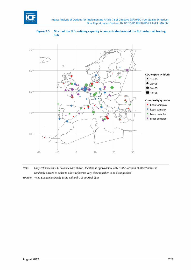
Impact Analysis of Options for Implementing Article 7a of Directive 98/70/EC (Fuel Quality Directive) Final Report under Contract 071201/2011/608705/SER/CLIMA.C2
August 2013 209
Figure 7.5 Much of the EU’s refining capacity is concentrated around the Rotterdam oil trading hub
Note: Only refineries in EU countries are shown; location is approximate only as the location of all refineries is
randomly altered in order to allow refineries very close together to be distinguished
Source: Vivid Economics partly using Oil and Gas Journal data
30
40
50
60
70
-20 -10 0 10 20 30
CDU capacity (b/cd)
1e+05
2e+05
3e+05
4e+05
Complexity quartile
Least complex
Less complex
More complex
Most complex

Impact Analysis of Options for Implementing Article 7a of Directive 98/70/EC (Fuel Quality Directive) Final Report under Contract 071201/2011/608705/SER/CLIMA.C2
August 2013 210
Figure 7.6 Around half of the EU’s refineries have a crude distillation capacity of between 50 and 150 thousand barrels per calendar day
Source: Vivid Economics from Oil and Gas Journal data
Refinery ownership can be classified according to a number of possible types:
– those refineries largely owned or controlled by one of the six oil majors (BP, Chevron,
the former ConocoPhilips, ExxonMobil, Shell, Total);
– those refineries largely owned or controlled by governments (such as Saudi Aramco or
Statoil);
– those refineries largely owned or controlled by specialist refining companies (such as
Valero, Tesoro, or the former Petroplus); and
– those refineries largely owned or controlled by independent operators.
There is overlap between these categories; for example, joint ventures between an oil major and a government-owned oil company. Furthermore, the precise shareholding of the holding company or companies responsible for a refinery is often complicated. Using publicly available information, each European refinery has been classified into one of these four categories, and the number of refineries and total crude distillation unit (CDU) capacity of each type is summarised in Figure 7.7 and Figure 7.8. Note that this information does not take into account changes in ownership which have occurred in the last twelve months.
0
5
10
15
20
25
0 50 100 150 200 250 300 350 400 450CDU capacity (kb/cd)
Nu
mb
er
of r
efin
eri
es

Impact Analysis of Options for Implementing Article 7a of Directive 98/70/EC (Fuel Quality Directive) Final Report under Contract 071201/2011/608705/SER/CLIMA.C2
August 2013 211
Figure 7.7 Independent owners account for around 40 per cent of the total number of refineries in the EU
Source: Vivid Economics based on Oil and Gas Journal data and various online sources
Figure 7.8 The six oil majors account for a greater share of refining capacity than their share of the number of refineries in the EU
Source: Vivid Economics based on Oil and Gas Journal data and various online sources
7.2.2 Demand for refined products
Global refined product demand has grown by 30 per cent over the past two decades, with the majority of this growth being in Asia, excluding Japan. Figure 7.9 illustrates demand growth over the past 25 years for five major consumption regions.
0
10
20
30
40
BP Chevron ConocoPhillips ExxonMobil Government Independent Shell Specialist TotalOwner category
Nu
mb
er
of r
efin
eri
es
0
2
4
6
BP Chevron ConocoPhillips ExxonMobil Government Independent Shell Specialist TotalOwner category
To
tal C
DU
ca
pa
city
(
mill
ion
ba
rre
ls p
er
da
y)

Impact Analysis of Options for Implementing Article 7a of Directive 98/70/EC (Fuel Quality Directive) Final Report under Contract 071201/2011/608705/SER/CLIMA.C2
August 2013 212
Figure 7.9 Fuel demand has risen sharply outside Europe, the US and Japan over the last decade
Note: PADD5 is the West Coast of the USA, while PADD123 refers to the US East Coast, Gulf Coast and Midwest
combined
Source: Vivid Economics from IEA and EIA data
Diesel, gasoline and residual fuel oil are the main products from refineries in the EU. The mix of refined product has changed over the last two decades. Distillate fuel oil output has grown while gasoline has fallen over the past decade, as Figure 7.10 shows.
Figure 7.10 Distillate fuel oil has seen growth in demand in Europe, while fuel oil and, recently, gasoline, have seen reductions in demand
Source EIA
0
2000
4000
6000
1970 1980 1990 2000 2010Year
De
ma
nd
in O
EC
D E
uro
pe
(ki
lob
arr
els
pe
r d
ay)
Product
Gas/diesel oil demand
Motor gasoline demand
Residual fuel oil demand
250000
500000
750000
1000000
1990 1995 2000 2005Year
To
tal f
ue
l de
ma
nd
(kt
pa
)
Market
Europe
Japan
Other
PADD5
PADD123
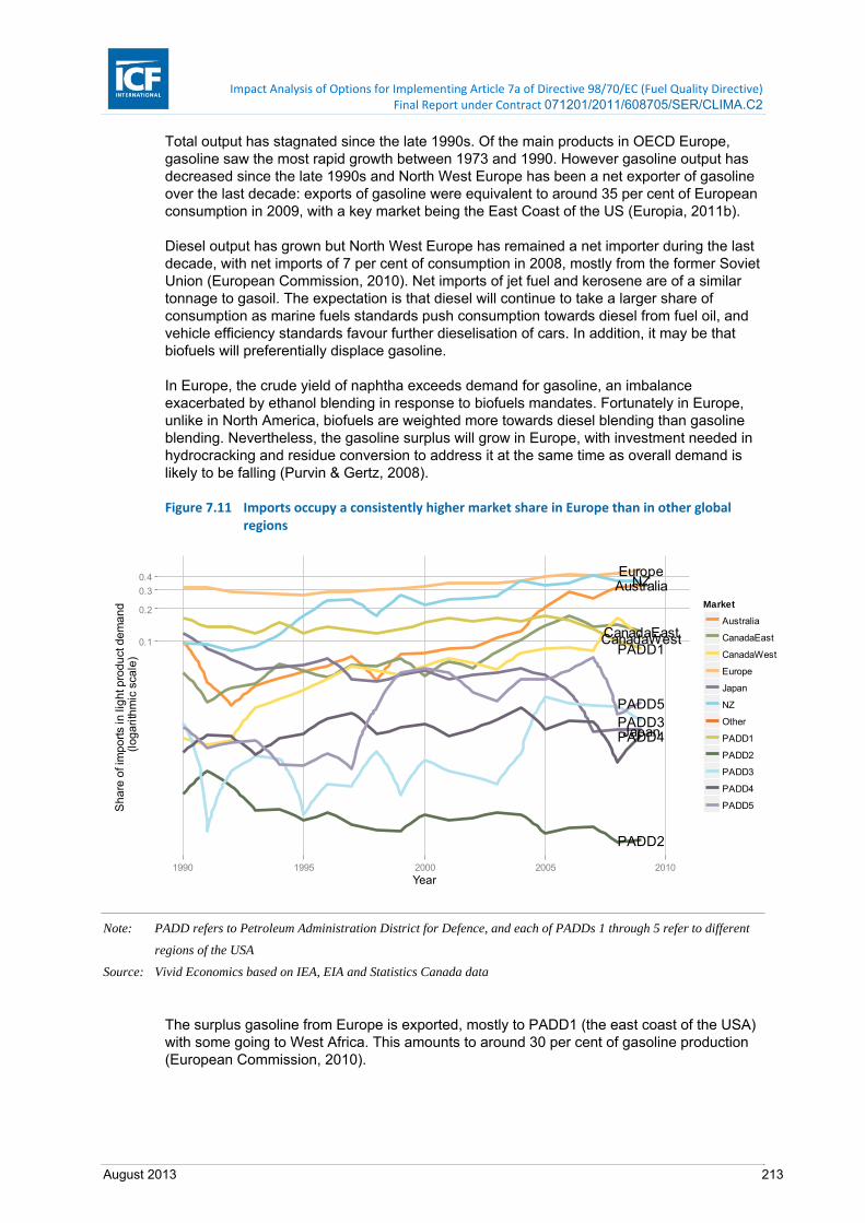
Impact Analysis of Options for Implementing Article 7a of Directive 98/70/EC (Fuel Quality Directive) Final Report under Contract 071201/2011/608705/SER/CLIMA.C2
August 2013 213
Total output has stagnated since the late 1990s. Of the main products in OECD Europe, gasoline saw the most rapid growth between 1973 and 1990. However gasoline output has decreased since the late 1990s and North West Europe has been a net exporter of gasoline over the last decade: exports of gasoline were equivalent to around 35 per cent of European consumption in 2009, with a key market being the East Coast of the US (Europia, 2011b).
Diesel output has grown but North West Europe has remained a net importer during the last decade, with net imports of 7 per cent of consumption in 2008, mostly from the former Soviet Union (European Commission, 2010). Net imports of jet fuel and kerosene are of a similar tonnage to gasoil. The expectation is that diesel will continue to take a larger share of consumption as marine fuels standards push consumption towards diesel from fuel oil, and vehicle efficiency standards favour further dieselisation of cars. In addition, it may be that biofuels will preferentially displace gasoline.
In Europe, the crude yield of naphtha exceeds demand for gasoline, an imbalance exacerbated by ethanol blending in response to biofuels mandates. Fortunately in Europe, unlike in North America, biofuels are weighted more towards diesel blending than gasoline blending. Nevertheless, the gasoline surplus will grow in Europe, with investment needed in hydrocracking and residue conversion to address it at the same time as overall demand is likely to be falling (Purvin & Gertz, 2008).
Figure 7.11 Imports occupy a consistently higher market share in Europe than in other global regions
Note: PADD refers to Petroleum Administration District for Defence, and each of PADDs 1 through 5 refer to different
regions of the USA
Source: Vivid Economics based on IEA, EIA and Statistics Canada data
The surplus gasoline from Europe is exported, mostly to PADD1 (the east coast of the USA) with some going to West Africa. This amounts to around 30 per cent of gasoline production (European Commission, 2010).
Australia
CanadaEastCanadaWest
Europe
Japan
NZ
PADD1
PADD2
PADD3PADD4
PADD5
0.1
0.2
0.3
0.4
1990 1995 2000 2005 2010Year
Sh
are
of i
mp
ort
s in
lig
ht p
rod
uct
de
ma
nd
(
log
ari
thm
ic s
cale
)
Market
Australia
CanadaEast
CanadaWest
Europe
Japan
NZ
Other
PADD1
PADD2
PADD3
PADD4
PADD5
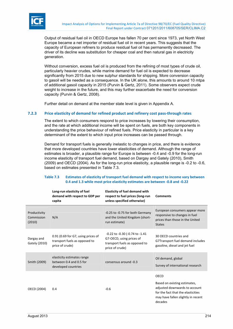
Impact Analysis of Options for Implementing Article 7a of Directive 98/70/EC (Fuel Quality Directive) Final Report under Contract 071201/2011/608705/SER/CLIMA.C2
August 2013 214
Output of residual fuel oil in OECD Europe has fallen 70 per cent since 1973, yet North West Europe became a net importer of residual fuel oil in recent years. This suggests that the capacity of European refiners to produce residual fuel oil has permanently decreased. The driver of its decline was substitution for cheaper coal and then natural gas in electricity generation.
Without conversion, excess fuel oil is produced from the refining of most types of crude oil, particularly heavier crudes, while marine demand for fuel oil is expected to decrease significantly from 2015 due to new sulphur standards for shipping. More conversion capacity to gasoil will be needed as a consequence. In the UK alone, this amounts to around 10 mtpa of additional gasoil capacity in 2015 (Purvin & Gertz, 2011). Some observers expect crude weight to increase in the future, and this may further exacerbate the need for conversion capacity (Purvin & Gertz, 2008).
Further detail on demand at the member state level is given in Appendix A.
7.2.3 Price elasticity of demand for refined product and refinery cost pass‐through rates
The extent to which consumers respond to price increases by lowering their consumption, and the rate at which additional income will be spent on fuels, are both key components in understanding the price behaviour of refined fuels. Price elasticity in particular is a key determinant of the extent to which input price increases can be passed through.
Demand for transport fuels is generally inelastic to changes in price, and there is evidence that more developed countries have lower elasticities of demand. Although the range of estimates is broader, a plausible range for Europe is between -0.4 and -0.9 for the long-run income elasticity of transport fuel demand, based on Dargay and Gately (2010), Smith (2009) and OECD (2004). As for the long-run price elasticity, a plausible range is -0.2 to -0.6, based on estimates presented in Table 7.3.
Table 7.3 Estimates of elasticity of transport fuel demand with respect to income vary between 0.4 and 1.3 while most price elasticity estimates are between ‐0.8 and ‐0.22
Long‐run elasticity of fuel
demand with respect to GDP per
capita
Elasticity of fuel demand with
respect to fuel prices (long‐run
unless specified otherwise)
Comments
Productivity
Commission
(2010)
N/A
‐0.25 to ‐0.75 for both Germany
and the United Kingdom (short‐
run estimate)
European consumers appear more
responsive to changes in fuel
prices than those in the United
States
Dargay and
Gately (2010)
0.91 (0.69 for G7, using prices of
transport fuels as opposed to
price of crude)
‐0.22 to ‐0.30 (‐0.74 to ‐1.41
G7‐OECD, using prices of
transport fuels as opposed to
price of crude)
30 OECD countries and
G7Transport fuel demand includes
gasoline, diesel and jet fuel
Smith (2009)
elasticity estimates range
between 0.4 and 0.5 for
developed countries consensus around ‐0.3
Oil demand, global
Survey of international research
OECD (2004) 0.4 ‐0.6
OECD
Based on existing estimates,
adjusted downwards to account
for the fact that the elasticities
may have fallen slightly in recent
decades
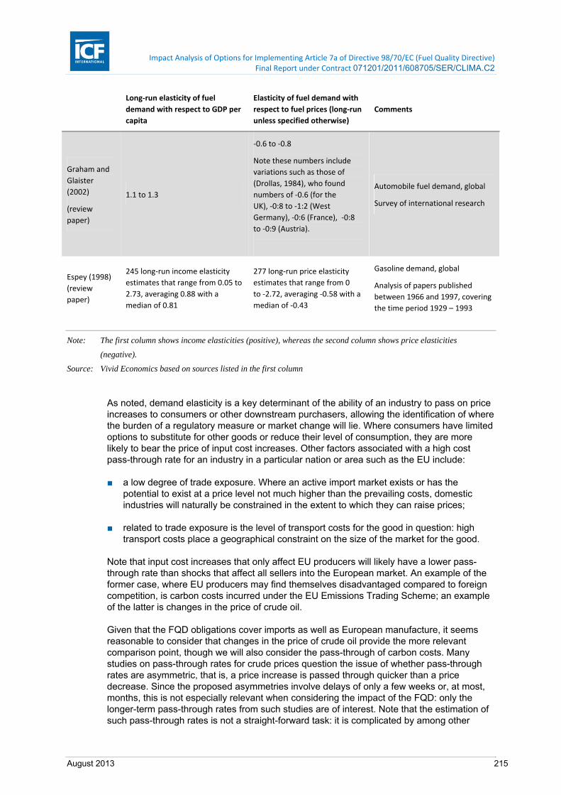
Impact Analysis of Options for Implementing Article 7a of Directive 98/70/EC (Fuel Quality Directive) Final Report under Contract 071201/2011/608705/SER/CLIMA.C2
August 2013 215
Long‐run elasticity of fuel
demand with respect to GDP per
capita
Elasticity of fuel demand with
respect to fuel prices (long‐run
unless specified otherwise)
Comments
Graham and
Glaister
(2002)
(review
paper)
1.1 to 1.3
‐0.6 to ‐0.8
Note these numbers include
variations such as those of
(Drollas, 1984), who found
numbers of ‐0.6 (for the
UK), ‐0:8 to ‐1:2 (West
Germany), ‐0:6 (France), ‐0:8
to ‐0:9 (Austria).
Automobile fuel demand, global
Survey of international research
Espey (1998)
(review
paper)
245 long‐run income elasticity
estimates that range from 0.05 to
2.73, averaging 0.88 with a
median of 0.81
277 long‐run price elasticity
estimates that range from 0
to ‐2.72, averaging ‐0.58 with a
median of ‐0.43
Gasoline demand, global
Analysis of papers published
between 1966 and 1997, covering
the time period 1929 – 1993
Note: The first column shows income elasticities (positive), whereas the second column shows price elasticities
(negative).
Source: Vivid Economics based on sources listed in the first column
As noted, demand elasticity is a key determinant of the ability of an industry to pass on price increases to consumers or other downstream purchasers, allowing the identification of where the burden of a regulatory measure or market change will lie. Where consumers have limited options to substitute for other goods or reduce their level of consumption, they are more likely to bear the price of input cost increases. Other factors associated with a high cost pass-through rate for an industry in a particular nation or area such as the EU include:
■ a low degree of trade exposure. Where an active import market exists or has the potential to exist at a price level not much higher than the prevailing costs, domestic industries will naturally be constrained in the extent to which they can raise prices;
■ related to trade exposure is the level of transport costs for the good in question: high transport costs place a geographical constraint on the size of the market for the good.
Note that input cost increases that only affect EU producers will likely have a lower pass-through rate than shocks that affect all sellers into the European market. An example of the former case, where EU producers may find themselves disadvantaged compared to foreign competition, is carbon costs incurred under the EU Emissions Trading Scheme; an example of the latter is changes in the price of crude oil.
Given that the FQD obligations cover imports as well as European manufacture, it seems reasonable to consider that changes in the price of crude oil provide the more relevant comparison point, though we will also consider the pass-through of carbon costs. Many studies on pass-through rates for crude prices question the issue of whether pass-through rates are asymmetric, that is, a price increase is passed through quicker than a price decrease. Since the proposed asymmetries involve delays of only a few weeks or, at most, months, this is not especially relevant when considering the impact of the FQD: only the longer-term pass-through rates from such studies are of interest. Note that the estimation of such pass-through rates is not a straight-forward task: it is complicated by among other

Impact Analysis of Options for Implementing Article 7a of Directive 98/70/EC (Fuel Quality Directive) Final Report under Contract 071201/2011/608705/SER/CLIMA.C2
August 2013 216
things, shifts in demand for the various fuels derived from crude, with the consequent differing price movements obscuring the contribution made by input cost changes.
Nonetheless, numerous studies covering time periods both in the EU and outside of it find high rates of pass-through. All the studies listed here are based on econometric studies:
■ (Bacon, 1990), in one of the early econometric studies on the subject, failed to reject the hypothesis of complete pass-through for the UK in the 1980s;
■ (Clerides, 2010), estimated pass-through rates for individual European countries that, for dates between 2000 and 2010, almost all tend to be close to 100 per cent;
■ likewise, Meyler, 2009, also finds evidence for complete pass-through in the EU, with 90 per cent of the retail price change occurring with three to five week;
■ for comparison, in the US context, (Bachmeier & Griffin, 2003), also estimated 100 per cent pass-through from 1985 to 1998.
Several studies have looked at the separate issue of the impact of a price change specific to the EU – that is, the EU Emissions Trading Scheme – on retail fuel prices. Such estimates include:
■ (Alexeeva-Talebi, 2011), uses time-series techniques to generate estimates of elasticities of petrol prices with relation to EUA prices that ‘are consistent’ with full cost pass-through. The results suggest that across EU countries, the elasticities of fuel prices with respect to carbon prices is around 0.01 to 0.09 per cent. Alexeeva-Talebi notes that if carbon costs make up, say, 2 per cent of total expenses (consistent with a net-of-tax retail price of 550 Euro/1,000L, and a carbon cost of 20 Euro/tonne), then this implies pass-through rates ranging from 50 to several hundred per cent. (Alexeeva-Talebi, 2011)
■ (Oberndorfer, et al., 2010), focusing on the UK, find elasticities for retail gasoline prices with regards to carbon prices of 0.01 to 0.03, and for diesel of 0.03 to 0.06. Again, assuming carbon costs are 2 per cent of total expenses, these pass-through rates span a range from 50 to several hundred per cent.
Contrary to intuition, pass-through rates of over 100 per cent are possible, so long as producers possess some degree of market power and the demand curve possesses a particular shape.88 Given, however, that in any case the cost-pass through rates for crude oil are more relevant, it appears that the true pass-through rate lies between 90 and 100 per cent.
A caveat to such estimates is that they may not be valid over a period of years or especially decades: over such timeframes, consumers have more scope to change their behaviour, both through changing the mix of currently employed technologies and by developing and adopting new technologies.
7.2.4 Profit margins in European refining
Refinery margins have moved between extremes over the last 20 years. A brief period of high margins from around 2005 ended with the advent of recession in North America and Europe in 2008, as demand fell for all products. Figure 7.12 shows refinery margins for refineries in North-west Europe, differentiating between those which can be characterised as hydroskimming and those that can be characterised as cracking. Typically crackers are indicative of a refinery type of medium complexity, while hydroskimming refineries are of low complexity. These less complex refineries are less able to take advantage of changes in
88 A study by CE Delft, (De Bruyn, et al., 2010), also find cost pass-through rates of several hundred per cent, despite their analysis suggesting that the EU refining market is strongly internationally integrated.
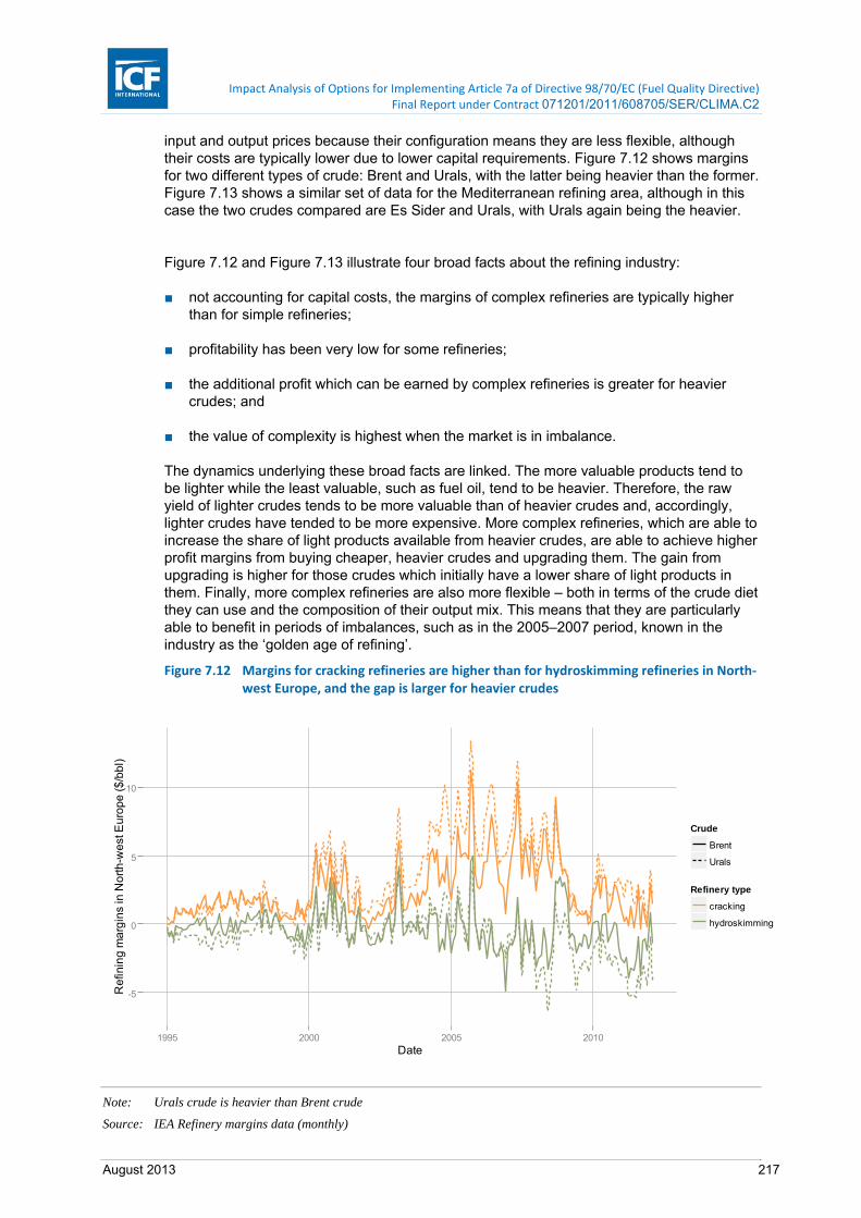
Impact Analysis of Options for Implementing Article 7a of Directive 98/70/EC (Fuel Quality Directive) Final Report under Contract 071201/2011/608705/SER/CLIMA.C2
August 2013 217
input and output prices because their configuration means they are less flexible, although their costs are typically lower due to lower capital requirements. Figure 7.12 shows margins for two different types of crude: Brent and Urals, with the latter being heavier than the former. Figure 7.13 shows a similar set of data for the Mediterranean refining area, although in this case the two crudes compared are Es Sider and Urals, with Urals again being the heavier.
Figure 7.12 and Figure 7.13 illustrate four broad facts about the refining industry:
■ not accounting for capital costs, the margins of complex refineries are typically higher than for simple refineries;
■ profitability has been very low for some refineries;
■ the additional profit which can be earned by complex refineries is greater for heavier crudes; and
■ the value of complexity is highest when the market is in imbalance.
The dynamics underlying these broad facts are linked. The more valuable products tend to be lighter while the least valuable, such as fuel oil, tend to be heavier. Therefore, the raw yield of lighter crudes tends to be more valuable than of heavier crudes and, accordingly, lighter crudes have tended to be more expensive. More complex refineries, which are able to increase the share of light products available from heavier crudes, are able to achieve higher profit margins from buying cheaper, heavier crudes and upgrading them. The gain from upgrading is higher for those crudes which initially have a lower share of light products in them. Finally, more complex refineries are also more flexible – both in terms of the crude diet they can use and the composition of their output mix. This means that they are particularly able to benefit in periods of imbalances, such as in the 2005–2007 period, known in the industry as the ‘golden age of refining’.
Figure 7.12 Margins for cracking refineries are higher than for hydroskimming refineries in North‐west Europe, and the gap is larger for heavier crudes
Note: Urals crude is heavier than Brent crude
Source: IEA Refinery margins data (monthly)
-5
0
5
10
1995 2000 2005 2010Date
Re
finin
g m
arg
ins
in N
ort
h-w
est
Eu
rop
e (
$/b
bl)
Crude
Brent
Urals
Refinery type
cracking
hydroskimming

Impact Analysis of Options for Implementing Article 7a of Directive 98/70/EC (Fuel Quality Directive) Final Report under Contract 071201/2011/608705/SER/CLIMA.C2
August 2013 218
Refinery markets are typically supra-national and somewhat regional. That said imbalances tend to persist for relatively short periods before they are closed through the arbitrage of oil traders and changes in refining activity. Figure 7.14 shows the margins for Urals crude in different refinery types in North-west Europe and the Mediterranean. Margins tend to follow a similar trajectory in both places, although differences can persist for periods of time.
Figure 7.13 Margins for cracking refineries are higher than for hydroskimming refineries in the Mediterranean with the difference being larger for heavier crudes
Note: Urals crude is heavier than Es Sider crude
Source: IEA Refinery margins data (monthly)
Figure 7.14 Refinery margins follow similar patterns in North‐west Europe and the Mediterranean and tend to be higher in North‐west Europe
Note: MED stands for Mediterranean while NWE stands for North-west Europe
Source: IEA Refinery margins data (monthly)
-5
0
5
10
1995 2000 2005 2010Date
Ref
inin
g m
arg
ins
in th
e M
ed
iterr
ane
an (
$/b
bl)
Refinery type
cracking
hydroskimming
Crude
Es.Sider
Urals
-5
0
5
10
1995 2000 2005 2010Date
Re
finin
g m
arg
ins
for
Ura
ls c
rud
e (
$/b
bl)
Refinery type
cracking
hydroskimming
Location
Med
NWE

Impact Analysis of Options for Implementing Article 7a of Directive 98/70/EC (Fuel Quality Directive) Final Report under Contract 071201/2011/608705/SER/CLIMA.C2
August 2013 219
European refining margins have been relatively low since the 1980s, but with periods of good profitability; see Figure 7.12, Figure 7.13 and Figure 7.14. The year 2009 saw some of the lowest margins in Europe for 15 years. This is partly due to refineries in Europe being less complex than those in some other neighbouring regions, such as North America, and older than those in other neighbouring regions such as the Middle East. Investment has taken place in Europe, but only where needed to ensure compliance with fuel quality standards. Most of the future investment required in Europe is driven by sulphur standards (CONCAWE., 2008). CONCAWE estimates this to be around $30 billion, with a similar amount to be spent on output barrel changes. The European Commission’s estimate of investment between 2005 and 2030 is lower, with around €4 billion to meet marine sulphur fuel specifications, out of a total investment requirement of €17.8 to 29.3 billion (European Commission, 2010).
The investment in additional complexity for fuel quality and conversion has been directed to the larger refineries so that refineries are usually now either large and complex or small and simple, as shown in Figure 7.15.
Figure 7.15 Smaller refineries are often less complex than larger ones
Source: Vivid Economics from Oil and Gas Journal data
7.2.5 Complexity of EU refineries
In the refining industry, refineries are often described according to their complexity. A complexity index describes the secondary conversion capacity of a refinery relative to the primary distillation capacity. Each piece of equipment which could be used in a refinery is given a factor which is then used to create a weighted average for each refinery. Further details of this calculation are given in Appendix A. A refinery with a greater complexity index generally has the following characteristics:
Size
Co
mpl
exity
Smallest Small Large Largest
Lea
st c
omp
lex
Less
com
ple
xM
ost
co
mp
lex
0.0
0.2
0.4
0.6
0.8
1.0

Impact Analysis of Options for Implementing Article 7a of Directive 98/70/EC (Fuel Quality Directive) Final Report under Contract 071201/2011/608705/SER/CLIMA.C2
August 2013 220
■ an ability to process heavier or lower quality crudes;
■ an ability to make products with more precise specifications, such as lower sulphur content;
■ greater scope to vary the composition of output, such as producing more diesel at the expense of gasoline when diesel prices are relatively high;
■ a higher capital cost; and
■ a higher average emissions intensity.
The complexity index used in this report is similar to the Nelson Complexity Index used by the industry, although the precise formula of the latter is not publicly available (Reliance Industries, 2006). Refineries in Europe typically have a lower complexity index than those in the United States, due to the availability of North Sea crude which reduces the need to process heavy crudes, and a ready market, at least for those refineries located on the coast, for marine fuel oil. The marine oil would otherwise be converted into other transport fuels using complex units.
The Fuel Quality Directive is likely to have a different impact on simple and complex refineries, and the potential impact could vary substantially depending upon the manner in which the Directive is implemented. Complex refineries gain a competitive advantage from being able to use low quality and heavier crudes, which are typically cheaper, yet still produce a product mix with large shares of valuable light products such as gasoline and diesel. Some of the implementation options for the Fuel Quality Directive may result in these crudes being associated with a cost penalty, which would generally hit complex refineries harder than simple ones.
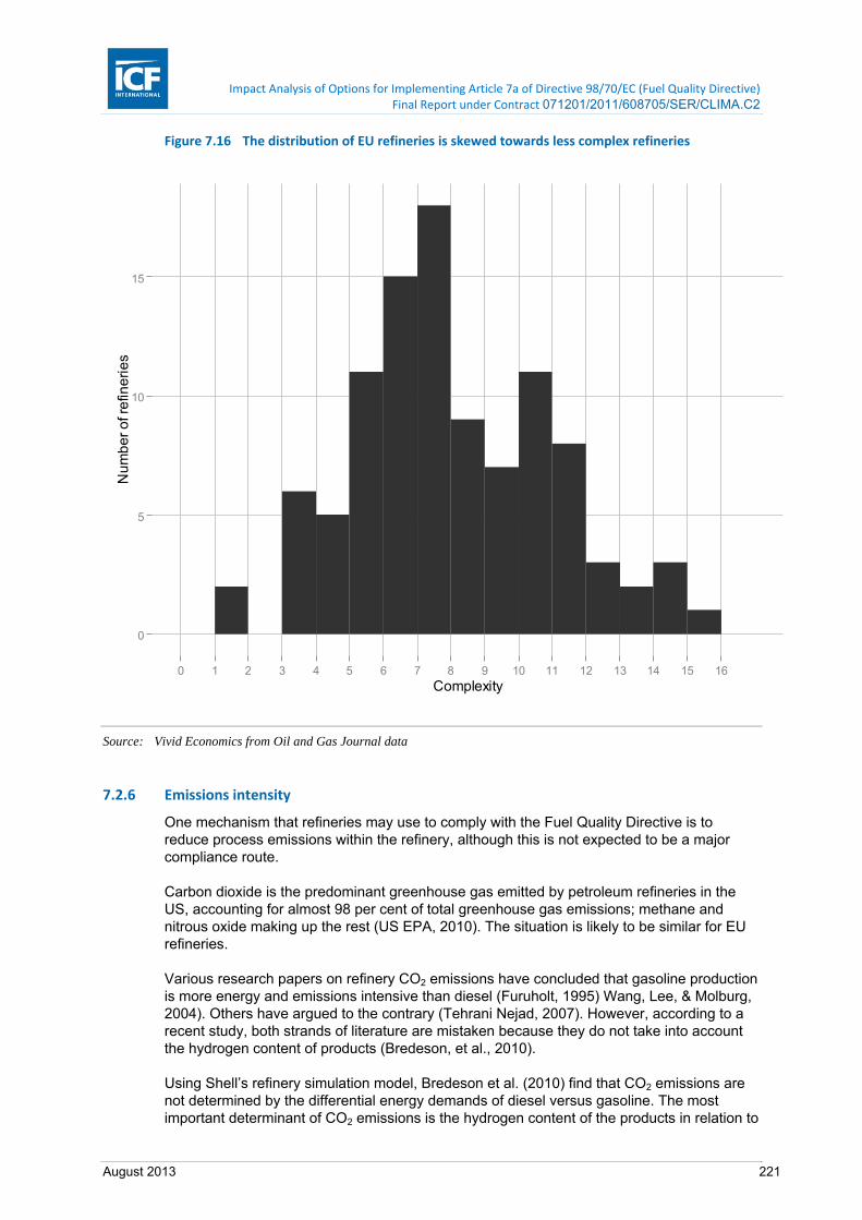
Impact Analysis of Options for Implementing Article 7a of Directive 98/70/EC (Fuel Quality Directive) Final Report under Contract 071201/2011/608705/SER/CLIMA.C2
August 2013 221
Figure 7.16 The distribution of EU refineries is skewed towards less complex refineries
Source: Vivid Economics from Oil and Gas Journal data
7.2.6 Emissions intensity
One mechanism that refineries may use to comply with the Fuel Quality Directive is to reduce process emissions within the refinery, although this is not expected to be a major compliance route.
Carbon dioxide is the predominant greenhouse gas emitted by petroleum refineries in the US, accounting for almost 98 per cent of total greenhouse gas emissions; methane and nitrous oxide making up the rest (US EPA, 2010). The situation is likely to be similar for EU refineries.
Various research papers on refinery CO2 emissions have concluded that gasoline production is more energy and emissions intensive than diesel (Furuholt, 1995) Wang, Lee, & Molburg, 2004). Others have argued to the contrary (Tehrani Nejad, 2007). However, according to a recent study, both strands of literature are mistaken because they do not take into account the hydrogen content of products (Bredeson, et al., 2010).
Using Shell’s refinery simulation model, Bredeson et al. (2010) find that CO2 emissions are not determined by the differential energy demands of diesel versus gasoline. The most important determinant of CO2 emissions is the hydrogen content of the products in relation to
0
5
10
15
0 1 2 3 4 5 6 7 8 9 10 11 12 13 14 15 16Complexity
Nu
mb
er
of r
efin
eri
es

Impact Analysis of Options for Implementing Article 7a of Directive 98/70/EC (Fuel Quality Directive) Final Report under Contract 071201/2011/608705/SER/CLIMA.C2
August 2013 222
the hydrogen content of the crude from which they were derived. More specifically, the following two factors are crucial:
■ first, the complexity of the refinery; in particular, whether it has a coker or other residue reduction unit to eliminate production of residual fuel. Carbon dioxide emissions increase as more transportation fuel is produced and correspondingly less residual fuel, because the coker not only consumes energy in its own right, but also because products resulting from residue reduction are of a lower quality, which requires units within the refinery to be upgraded.
■ second, crude heaviness; the heavier the crude, the higher the energy use, but only for complex refineries. In a refinery that has no coker, and thus produces a great deal of residual fuel, crude heaviness has little impact on total CO2 emissions. However, there is an indirect heavy crude CO2 penalty, because with no coker, more carbon-rich residual fuel leaves the refinery.
An equivalent explanation in terms of hydrogen is as follows. If the crude contains less hydrogen, that is, it is heavier, and/or the products have more hydrogen going out, that is, less residual fuel and more transport fuel, the total CO2 emissions of the refinery will be higher.
Other slightly less important factors include (Bredeson, et al., 2010); (Delucchi, 2005)):
■ type of crude: naphthenic or paraffinic, since CO2 emissions and energy consumptions are slightly higher for naphthenic crudes;
■ product specification changes resulting from tightened regulations: lower sulphur or lower aromatics, the production of which would raise CO2 emissions;
■ liquid petroleum gas production, because refineries which make more LPG have higher CO2 emissions. That being said, refineries cannot lower LPG production by much, and they cannot make less LPG, as its output is usually minimised;
■ degree of energy or carbon conservation. Examples include use of high efficiency motors, variable speed drives, carbon capture techniques;
■ shifts in demand for and resulting changes in refinery production of one petroleum product, for example, if demand for gasoline falls, the refinery may start producing more diesel, possibly raising emissions; and
■ forcing production ratios outside ‘normal ranges’; when a refinery is pushed to make more of a particular fuel, its CO2 emissions increase.
It is a significant challenge to take differences in emissions intensities in the refinery and apply them to the requirements of the Fuel Quality Directive for particular fuels. This is because it is extremely difficult to allocate emissions from a refinery to particular products due to the joint nature of production and the multiple purposes to which many emissions-intensive units are put (Bredeson, et al., 2010).
A further barrier in the consideration of refinery process emissions is that data on the emissions intensity of non-EU refineries is difficult to obtain (see e.g. Section 5.3).
In order to provide some insight into the relationships between refinery size, complexity and emissions, data from the EU ETS has been matched with the refinery database constructed for this report (although more checking needs to be done on the matching before the final report). Larger refineries tend to have higher emissions (see Figure 7.17), which suggest that on an average basis emissions may be somewhat proportional to output. However, it is important to note that it may not be the case that marginal emissions are proportional to

Impact Analysis of Options for Implementing Article 7a of Directive 98/70/EC (Fuel Quality Directive) Final Report under Contract 071201/2011/608705/SER/CLIMA.C2
August 2013 223
marginal output, and that this can have an important impact upon the competitive impact of regulations.
Figure 7.18 considers the emissions intensity of a refinery. This is calculated in relation to the capacity of a refinery rather than output, because data on output is not publicly available at the refinery level. This means that some of the differences in emissions intensity per unit of capacity may be due to differences in capacity utilisation in a given year. Figure 7.18 indicates that a higher emissions intensity is typically associated with a higher complexity index. Some of the pieces of equipment associated with more complex refineries, such as cokers, are typically used to turn long-chain hydrocarbons into short chain hydrocarbons, which results in CO2 emissions.
Figure 7.17 Larger and more complex refineries tend to have higher emissions, although the relationship is not uniform
Source: Vivid Economics from Oil and Gas Journal and EC data
0e+00
2e+06
4e+06
6e+06
0e+00 1e+05 2e+05 3e+05 4e+05CDU capacity (b/cd)
EU
ET
S v
eri
fied
em
issi
on
s 2
01
1
4
8
12
Complexity

Impact Analysis of Options for Implementing Article 7a of Directive 98/70/EC (Fuel Quality Directive) Final Report under Contract 071201/2011/608705/SER/CLIMA.C2
August 2013 224
Figure 7.18 More complex refineries often, but not always, have a higher emissions intensity than less complex refineries
Source: Vivid Economics from Oil and Gas Journal and EC data
7.2.7 Trade in refined products
In 2010, the European Union imported 670 Mt of crude oil. Behind the aggregate figures, individual national trends exist. The Czech Republic, Greece, Lithuania, Romania and Poland for example have increased the volume of imports of crude oil; while in Spain, France, Germany and Italy the volume has decreased. The breakdown by country and the evolution over the past decade is presented in Appendix A in Table A1.10.
Russia is by far the largest source of imported crude into the EU, accounting for just less than 180,000 ktpa (kilotonnes per year) of imported crude, around 35 per cent of total imports into the EU. Norway and Libya were the second and third most important sources, accounting for around 13 and 10 per cent of imports, respectively.
0
10
20
30
4 8 12 16Complexity
EU
ET
S v
eri
fied
em
issi
on
s 2
01
1 p
er
cap
aci
ty b
arr
el

Impact Analysis of Options for Implementing Article 7a of Directive 98/70/EC (Fuel Quality Directive) Final Report under Contract 071201/2011/608705/SER/CLIMA.C2
August 2013 225
Figure 7.19 In 2010 Russia, Norway and Libya were the biggest sources of EU‐27 imports of crude oil
Note: Imports from the 15 largest sources are shown; total imports were around 520,000 ktpa
Source: Vivid Economics analysis of Eurostat data (series nrg_123a)
Table 7.4 Mad Dog, USA and Gullfaks, Norway are the oilfields with the lowest carbon intensity and highest API gravity in a sample of wellhead‐to‐refinery emissions calculations
Field API gravity Carbon intensity (g CO2/MJ)
Cantarell, Mexico 22 15.2
Mad Dog, USA 42 6.2
Steepbank/Millennium Mine, Canada 10 26.6
Hibernia, Canada 35 7.3
Kupal, Iran 32 30.5
Ghawar, Saudi Arabia 34 7.9
Dacion, Venezuela 20 22.0
Bu Attifel, Libya 41 6.9
Samotlor, Russia 34 11.8
Duri, Indonesia 22 14.3
Forties, UK 37 8.0
Gullfaks, Norway 41 6.2
Note: For simplification purposes, the authors assumed that energy use and GHG emissions in refining vary only
according to API gravity; the impact of sulphur content was not considered.
Source: (Energy Redefined, 2010), figures taken from table E1 on page 10 of the report
Russia
Norway
Libya
Saudi ArabiaIran KazakhstanNigeriaAzerbaijan
IraqAngola SyriaMexicoAlgeria VenezuelaBrazil
0
50000
100000
150000
Alg
eria
Ang
ola
Aze
rbai
jan
Bra
zil
Iran
Iraq
Kaz
akhs
tan
Liby
a
Mex
ico
Nig
eria
Nor
way
Rus
sia
Sau
di A
rabi
a
Syr
ia
Ven
ezue
la
Import source
Th
ou
san
ds
of t
on
ne
s o
f cru
de
pe
r ye
ar

Impact Analysis of Options for Implementing Article 7a of Directive 98/70/EC (Fuel Quality Directive) Final Report under Contract 071201/2011/608705/SER/CLIMA.C2
August 2013 226
Eurostat does not report the API gravity of the crude oil imported or its wellhead-to-refinery emissions, however estimates for representative oil fields do exist in the literature. Table 7.4 provides such examples for representative oil fields, taken from a study by Energy-Redefined LLC (Energy-Redefined, 2010). The report also estimates that 80 per cent of crude oil imported into the EU has an API gravity of 30 to 40.
Energy-Redefined (2010) estimated that extraction-to-refining emissions from crude oil imports into the EU were around 330 million tonnes of CO2e in 2010.
Table A1.11, in the Appendix, presents data on imports of motor gasoline by member state. The Netherlands, the UK and Germany imported the most in terms of volume: 9.9, 3.5 and 2.1Mt respectively. The breakdown by country of origin for imports into the EU-27 as a whole is provided in Figure 7.20. Imports accounted for less than two per cent of the EU’s gasoline demand in 2010.
Figure 7.20 Imports of gasoline into the EU account for a very small proportion of the approximately 400,000 kt of demand each year
Note: Total imports of motor gasoline in 2010 from outside of the EU were 7,495 ktpa out of a total demand of around
400,000 ktpa
Source: Vivid Economics analysis of Eurostat data (series nrg_123a)
A summary by member state of imports of diesel and gas oil is presented in Table A1.11 in the Appendix, and a summary at the EU level is shown in Figure 7.21. When reporting imports and exports of diesel by country of origin, Eurostat provides a combined figure for gas and diesel oil.89 The shares by country of origin in Figure 7.21 refer to this gas and diesel oil. These shares might also offer a good indication of transport diesel shares if the ratio of diesel to gas oil imports does not vary too much by country.
Russia is, by some distance, the major source of diesel imports into the EU, with the USA and India also being major sources; these three accounted for around 40, 15 and 11 per cent of total diesel/gas oil imports in 2010.
89 For example, EU-27 imports of gas/diesel oil were 117Mt in 2010; knowing that transport diesel imports were 79Mt, this
implies imports of heating oil amounted to 38Mt.
Not specified
Norway
Russia United StatesOther AmericaOther EuropeOther AfricaNigeriaCroatia GeorgiaAlgeria Trinidad and TobagoSaudi ArabiaQatar Ukraine
0
1000
2000
3000
4000
5000
Alg
eria
Cro
atia
Geo
rgia
Nig
eria
Nor
way
Not
spe
cifie
d
Oth
er A
fric
a
Oth
er A
mer
ica
Oth
er E
urop
e
Qat
ar
Rus
sia
Sau
di A
rabi
a
Trin
idad
and
Tob
ago
Ukr
aine
Uni
ted
Sta
tes
Import source
Th
ou
san
ds
of t
on
ne
s o
f ga
solin
e p
er
yea
r
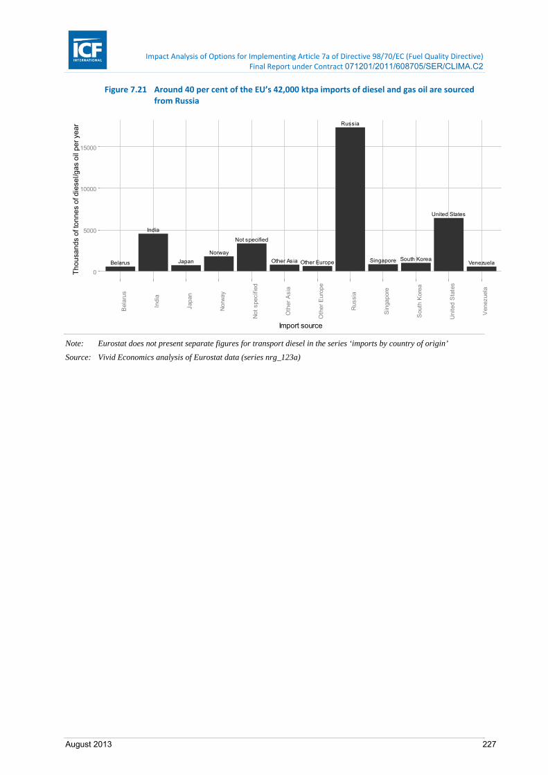
Impact Analysis of Options for Implementing Article 7a of Directive 98/70/EC (Fuel Quality Directive) Final Report under Contract 071201/2011/608705/SER/CLIMA.C2
August 2013 227
Figure 7.21 Around 40 per cent of the EU’s 42,000 ktpa imports of diesel and gas oil are sourced from Russia
Note: Eurostat does not present separate figures for transport diesel in the series ‘imports by country of origin’
Source: Vivid Economics analysis of Eurostat data (series nrg_123a)
Russia
United States
India
Not specified
NorwaySouth KoreaSingaporeOther AsiaJapan Other EuropeBelarus Venezuela
0
5000
10000
15000
Bel
arus
Indi
a
Japa
n
Nor
way
Not
spe
cifie
d
Oth
er A
sia
Oth
er E
urop
e
Rus
sia
Sin
gapo
re
Sou
th K
orea
Uni
ted
Sta
tes
Ven
ezue
la
Import source
Th
ou
san
ds
of t
on
ne
s o
f die
sel/g
as
oil
pe
r ye
ar

Impact Analysis of Options for Implementing Article 7a of Directive 98/70/EC (Fuel Quality Directive) Final Report under Contract 071201/2011/608705/SER/CLIMA.C2
August 2013 228
8 Impacts of the Fuel Quality Directive on the EU road transport fuel market (Task 3.2)
8.1 Introduction
The Directive could have a number of potential impacts on international competitiveness in the supply chain, particularly in refining. This study seeks to establish, through economic modelling, the likely magnitude of these effects.
The Directive affects upstream and downstream markets. The impacts would be felt both by EU and non-EU feedstock producers, refiners and EU consumers of refined product. The ultimate incidence of any regulatory cost along the value chain depends upon the nature of the regulation and on the economic characteristics of the market.
The sequence by which the impacts present themselves can be understood as follows. Suppliers compete in the market and are subject to unequal cost increases induced by the Directive. The Directive causes the costs of some suppliers to increase by some amount more than others and various consequences follow.
A stylised picture of the value chain which forms the basis for the analysis is presented in Figure 8.1. Feedstock and blending component suppliers, each with its own market share and costs of production, compete in order to supply raw materials to fuel suppliers. Fuel suppliers, with a similar diversity of costs and market shares, also compete. Finally, buyers of finished product react to any cost changes passed down the value chain.
The changed competitive position of market participants at each step of the value chain causes market shares to shift between them. The manner in which the Directive is implemented would affect the size of these cost increases, and therefore of the changed competitive position. The increase in cost of supply pushes up the price of the final product and, in response, the quantity demanded decreases. The size of the final price increase depends upon the extent to which firms are able to pass on the increased costs, which depends both on competitive conditions and the sensitivity of consumer demand to prices. Figure 8.2 depicts these interactions.
Figure 8.1 Value chain of fuel supply in the EU
Source: Vivid Economics

Impact Analysis of Options for Implementing Article 7a of Directive 98/70/EC (Fuel Quality Directive) Final Report under Contract 071201/2011/608705/SER/CLIMA.C2
August 2013 229
Figure 8.2 Dynamics of changes in competition
Source: Vivid Economics
The distribution and magnitude of impacts can be described and in this case they can be estimated. Nearly all the costs of the scheme are ultimately borne by consumers. Those who gain from the scheme are producers of advantaged feedstocks and refiners better suited to those feedstocks, who gain both in terms of market share and profit margin. Those who lose are the producers of disadvantaged feedstocks and refiners better suited to those feedstocks.
8.2 Main results
Compliance costs are largely driven by the availability of Upstream Emissions Reductions (UERs) and biofuels. Figure 8.3 shows the abatement potential of each and their unit costs. Crude and product selection have less potential than UERs and biofuels by an order of magnitude.

Impact Analysis of Options for Implementing Article 7a of Directive 98/70/EC (Fuel Quality Directive) Final Report under Contract 071201/2011/608705/SER/CLIMA.C2
August 2013 230
Figure 8.3 Most of the available abatement stems from UERs and biofuels
Note: non-ILUC compliance cost curves. Product and crude selection show full differentiation as allowed under
option 5. The potential for product and/or crude selection is lower in options 3 and 1.The steeper slope
for product selection after 0.9mtCO2e is explained by the exit of diesel derived from unconventional
feedstocks and the remaining part from 0.9 to 1.2mtCO2e is achieved by selecting between diesel
derived from conventional feedstocks.
Source: Vivid Economics; ICF
UERs and biofuels account for over 90 per cent of all abatement potential. UERs provide approximately 75 per cent of all abatement potential for any ceiling on unit costs. This is the case in both the non-ILUC (Including Land Use Change) and ILUC scenario as seen in Figure 8.4 and Figure 8.5.
UER
0
50
100
150
200
0 10 20 30Abatement potential (mtCO2e)
Co
st (
Eu
r/tC
O2
e)
Biofuels
0
100
200
0 5 10 15 20Abatement potential (mtCO2e)
Co
st (
Eu
r/tC
O2
e)
Product
0
100
200
300
0.0 0.3 0.6 0.9 1.2Abatement potential (mtCO2e)
Co
st (
Eu
r/tC
O2
e)
Crude
0
100
200
300
0.0 0.2 0.4 0.6 0.8Abatement potential (mtCO2e)
Co
st (
Eu
r/tC
O2
e)
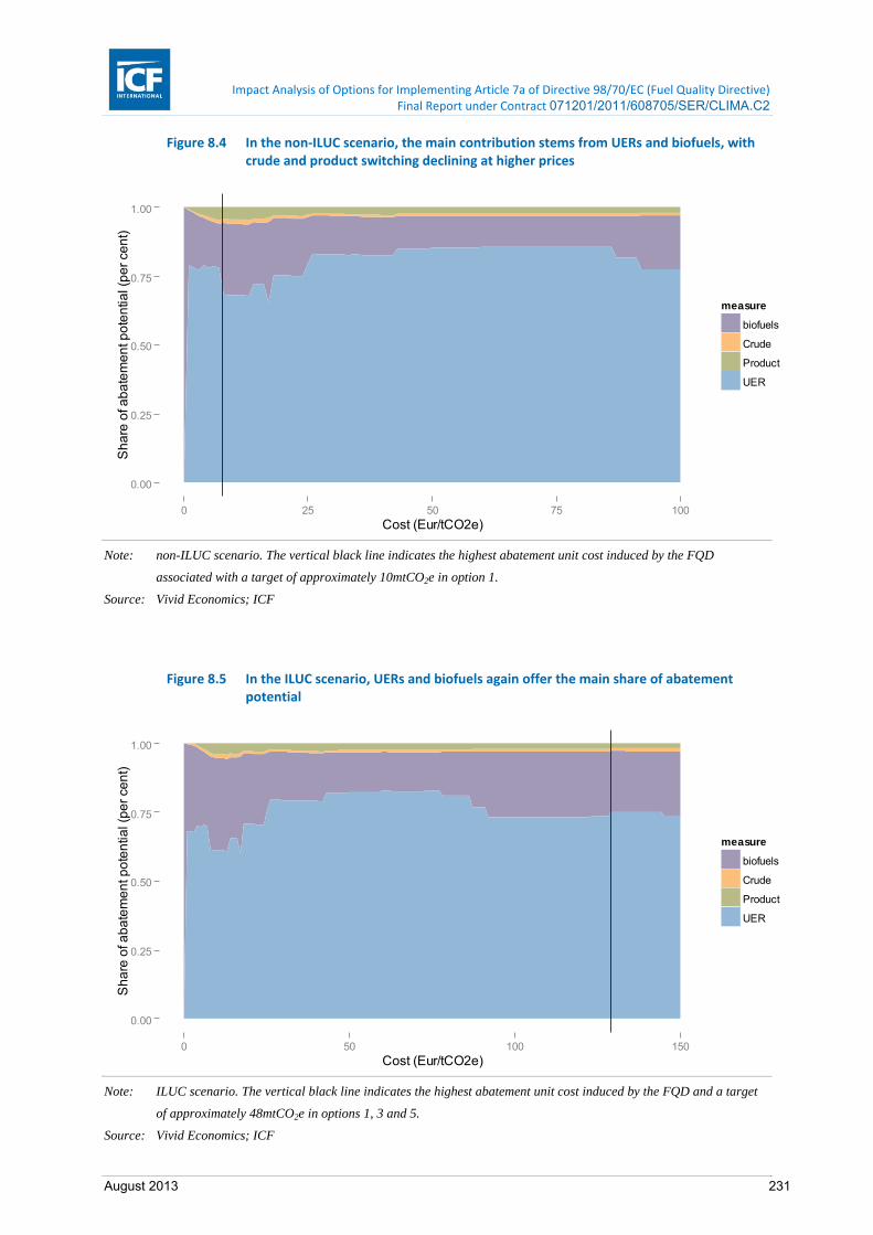
Impact Analysis of Options for Implementing Article 7a of Directive 98/70/EC (Fuel Quality Directive) Final Report under Contract 071201/2011/608705/SER/CLIMA.C2
August 2013 231
Figure 8.4 In the non‐ILUC scenario, the main contribution stems from UERs and biofuels, with crude and product switching declining at higher prices
Note: non-ILUC scenario. The vertical black line indicates the highest abatement unit cost induced by the FQD
associated with a target of approximately 10mtCO2e in option 1.
Source: Vivid Economics; ICF
Figure 8.5 In the ILUC scenario, UERs and biofuels again offer the main share of abatement potential
Note: ILUC scenario. The vertical black line indicates the highest abatement unit cost induced by the FQD and a target
of approximately 48mtCO2e in options 1, 3 and 5.
Source: Vivid Economics; ICF
0.00
0.25
0.50
0.75
1.00
0 25 50 75 100Cost (Eur/tCO2e)
Sh
are
of a
ba
tem
en
t po
ten
tial (
pe
r ce
nt)
measure
biofuels
Crude
Product
UER
0.00
0.25
0.50
0.75
1.00
0 50 100 150Cost (Eur/tCO2e)
Sh
are
of a
ba
tem
en
t po
ten
tial (
pe
r ce
nt)
measure
biofuels
Crude
Product
UER

Impact Analysis of Options for Implementing Article 7a of Directive 98/70/EC (Fuel Quality Directive) Final Report under Contract 071201/2011/608705/SER/CLIMA.C2
August 2013 232
If suppliers select the most cost-effective means of compliance, then the last compliance measure to be purchased will be at a unit cost which we shall term the market price for abatement. If the compliance obligations and measures are traded between participants then this may be an observable market price.
The market price for abatement is mainly influenced by the availability of UERs and biofuels. For each option’s abatement target, except non-ILUC option 3 full joint reporting, the marginal abatement stems from either biofuels in the non-ILUC scenario or from UERs in the ILUC scenario.
8.3 Required emissions reduction in the EU transport fossil fuel market
The FQD requires a reduction of approximately 10 to 50 MtCO2e of EU transport fuel emissions as compared with the 2020 baseline for the non-ILUC and ILUC scenario respectively. The emissions intensity of EU transport fuels in 2020 where the FQD target is not met is estimated to be approximately 83.76 gCO2e/MJ (if assuming the Commission’s proposed 2011 default values) or 83.95 gCO2e/MJ if assuming changes to the default unit intensities to reflect the estimated 2020 crude mix; the FQD requires a reduction to 83.002gCO2e/MJ. Table 8.1 shows the total abatement for the EU estimated to be required in 2020 for each policy option under the non-ILUC and ILUC scenario compared to the baseline. The calculation of both the initial intensity and the FQD target are laid out in earlier sections of this report.
Table 8.1 Switching from full joint reporting to individual reporting results in slightly higher abatement targets under the non‐ILUC scenario but no changes in the ILUC scenario, reduction in mtCO2e per annum
Scenario Reporting Option 0 Option 1 Option 2 Option 3 Option 5
non-ILUC
Full joint reporting reduction target 10.32 10.32 10.32 9.84 10.32
No joint reporting reduction target
10.45 10.81 10.81 10.33 10.82
ILUC Full joint/no joint reporting reduction target
48.08 48.08 48.08 47.54 48.08
Note: Required average EU emissions reductions under Option 3 are underestimated as suppliers whose fuel intensity is
above default values would effectively be allowed to report the lower default value.
Source: Vivid Economics; ICF
The economic analysis examines full joint reporting, which involves a marginally lower abatement in the non-ILUC scenario. The difference between full joint and no joint reporting is only significant if there is no market to trade emissions from transport fuel production. In reality, the most likely scenario is that each fuel producer will have the ability to either buy emissions reductions if their intensity is above the FQD target or sell surplus emissions if their intensity is below the target. If this market exists, the difference between full joint and no joint reporting vanishes.

Impact Analysis of Options for Implementing Article 7a of Directive 98/70/EC (Fuel Quality Directive) Final Report under Contract 071201/2011/608705/SER/CLIMA.C2
August 2013 233
8.4 Analysis of options
The main results are:
■ abatement costs are between €6/tCO2e and €7.7/tCO2e in the non-ILUC scenario and between €129/tCO2e and €145/tCO2e in the ILUC scenario;
■ European transport fossil fuel demand declines by around 0.1 per cent and approximately 0.5 per cent in the non-ILUC and ILUC scenario respectively compared with the baseline;
■ unconventional crude use in the EU declines by approximately 3 per cent in the non-ILUC scenario when crude switching is allowed and 20 per cent in the ILUC when crude selection scenario is allowed compared with the baseline pre-FQD crude mix;
■ imports of diesel derived from unconventional feedstocks declines by between 30 and 35 per cent in the non-ILUC scenario when product selection is allowed and by 100 per cent in the ILUC scenario when product switching is allowed compared with the baseline pre-FQD diesel imports;
■ policy options 1, 3 and 5 reduce imports of high emissions intensity transport fossil fuels more than options 0 and 2;
■ pump prices rise by approximately 0.03 per cent, in the non-ILUC scenario and by up to about 2.3 per cent, in the ILUC scenario;
■ there is no difference in the number of refinery exits between the policy options within the non-ILUC and ILUC scenarios;
■ there is no difference to the cost of capital, the cost of labour, employment, value added and capacity to innovate in the EU refining sector between the different policy options within the non-ILUC and ILUC scenarios;
■ under full joint reporting, fuel suppliers with initial emissions intensities below the FQD target might benefit; and
8.4.1 Compliance cost curves
The compliance cost curves are driven by UERs and biofuels. Table 8.2 shows that UERs are contributing approximately 75 per cent of all abatement and biofuels, the remainder for options 0 and 2 and a larger part of the remainder for options 1, 3 and 5. Crude and product switching each contribute 5 per cent or less of all abatement.

Impact Analysis of Options for Implementing Article 7a of Directive 98/70/EC (Fuel Quality Directive) Final Report under Contract 071201/2011/608705/SER/CLIMA.C2
August 2013 234
Table 8.2 UERs contribute approximately 75 per cent of all abatement with biofuels contributing almost all of the remainder
Scenario Variable Option 0 Option 1 Option 2 Option 3 Option 5
non-ILUC
CO2 price (€/tCO2e) 7.7 7.7 7.7 6 7.7
UER contribution (per cent)
72 78 72 79 78
Biofuels contribution (per cent)
28 16 28 16 16
Crude selection contribution (per cent)
- 1 - 1 1
Product selection contribution (per cent)
- 5 - 4 5
ILUC
CO2 price (€/tCO2e) 145 129 145 129 129
UER contribution (per cent)
76 73 76 73 73
Biofuels contribution (per cent)
24 24 24 23 23
Crude selection contribution (per cent)
- 1 - 2 2
Product selection contribution (per cent)
- 2 - 2 2
Note: The CO2 price is the marginal price at which the required abatement for each option is achieved. A more
appropriate comparison of costs reflecting the lower environmental effectiveness of Option 3 would be to assume
that the CO2 price for this option lie in the range between those for option 1 and option 5.
Source: Vivid Economics; ICF
UERs are the predominant source of low cost abatement, with some biofuels being available at negative costs, as identified in Task 1. Figure 8.6 Figure 8.7 Figure 8.8 show that UERs are available at relatively large quantities at low prices. In addition, the figures show that in the non-ILUC scenario, biofuels provide the marginal abatement (except for option 3) and in the ILUC scenario UERs provide the marginal abatement for options 1, 3 and 5 and biofuels for options 0 and 2.
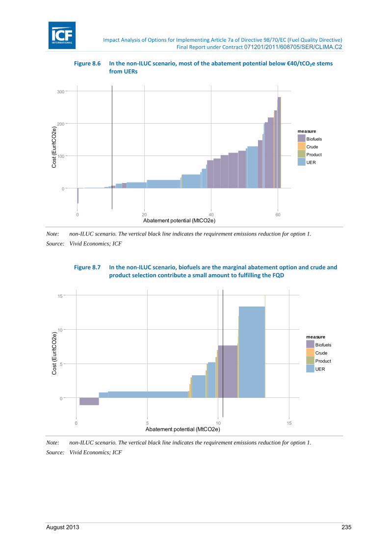
Impact Analysis of Options for Implementing Article 7a of Directive 98/70/EC (Fuel Quality Directive) Final Report under Contract 071201/2011/608705/SER/CLIMA.C2
August 2013 235
Figure 8.6 In the non‐ILUC scenario, most of the abatement potential below €40/tCO2e stems from UERs
Note: non-ILUC scenario. The vertical black line indicates the requirement emissions reduction for option 1.
Source: Vivid Economics; ICF
Figure 8.7 In the non‐ILUC scenario, biofuels are the marginal abatement option and crude and product selection contribute a small amount to fulfilling the FQD
Note: non-ILUC scenario. The vertical black line indicates the requirement emissions reduction for option 1.
Source: Vivid Economics; ICF
0
100
200
300
0 20 40 60Abatement potential (MtCO2e)
Co
st (
Eu
r/tC
O2
e)
measure
Biofuels
Crude
Product
UER
0
5
10
15
0 5 10 15Abatement potential (MtCO2e)
Co
st (E
ur/t
CO
2e
)
measure
Biofuels
Crude
Product
UER
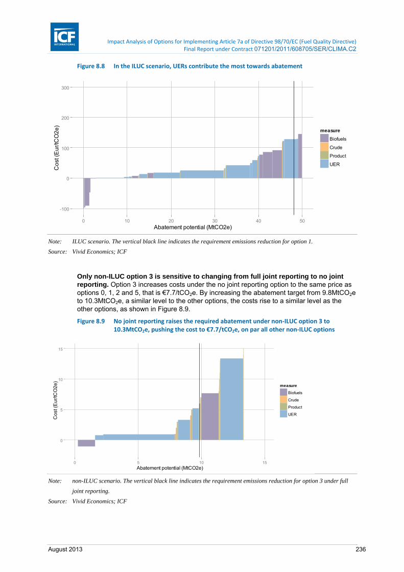
Impact Analysis of Options for Implementing Article 7a of Directive 98/70/EC (Fuel Quality Directive) Final Report under Contract 071201/2011/608705/SER/CLIMA.C2
August 2013 236
Figure 8.8 In the ILUC scenario, UERs contribute the most towards abatement
Note: ILUC scenario. The vertical black line indicates the requirement emissions reduction for option 1.
Source: Vivid Economics; ICF
Only non-ILUC option 3 is sensitive to changing from full joint reporting to no joint reporting. Option 3 increases costs under the no joint reporting option to the same price as options 0, 1, 2 and 5, that is €7.7/tCO2e. By increasing the abatement target from 9.8MtCO2e to 10.3MtCO2e, a similar level to the other options, the costs rise to a similar level as the other options, as shown in Figure 8.9.
Figure 8.9 No joint reporting raises the required abatement under non‐ILUC option 3 to 10.3MtCO2e, pushing the cost to €7.7/tCO2e, on par all other non‐ILUC options
Note: non-ILUC scenario. The vertical black line indicates the requirement emissions reduction for option 3 under full
joint reporting.
Source: Vivid Economics; ICF
-100
0
100
200
300
0 10 20 30 40 50Abatement potential (MtCO2e)
Co
st (
Eu
r/tC
O2
e)
measure
Biofuels
Crude
Product
UER
0
5
10
15
0 5 10 15Abatement potential (MtCO2e)
Co
st (
Eu
r/tC
O2
e)
measure
Biofuels
Crude
Product
UER

Impact Analysis of Options for Implementing Article 7a of Directive 98/70/EC (Fuel Quality Directive) Final Report under Contract 071201/2011/608705/SER/CLIMA.C2
August 2013 237
The exclusion of crude and product selection results in the same CO2 price and higher biofuel uptake in the non-ILUC scenario. Figure 8.10 shows that the exclusion of crude and product selection in the non-ILUC scenario results in a small shift of the compliance cost curve to the left. As the marginal abatement measure stems from biofuels, more biofuel is taken up.
Figure 8.10 In the non‐ILUC scenario, the exclusion of crude and product switching results in shifting the compliance curve marginally to the left and a higher uptake of biofuels in the marginal €7.7/tCO2e measure
Note: non-ILUC scenario. The vertical black line indicates the requirement emissions reduction for option 2.
Source: Vivid Economics; ICF
In the ILUC scenario, however, the exclusion of crude and product selection pushes up the CO2 price by over €15/tCO2 as additional UERs are needed to fulfil the FQD target. Figure 8.11 shows that the exclusion of crude and product selection raises the CO2 price by moving the marginal contribution from a UER measure to a biofuel measure. The additional biofuels become available at a higher cost of €145/tCO2e.
Figure 8.11 In the ILUC scenario, excluding crude and product selection results in a step up the compliance cost curve from €129/tCO2e to €145/tCO2e and additional biofuel blending
Note: ILUC scenario. The vertical black line indicates the requirement emissions reduction for option 2.
Source: Vivid Economics; ICF
-100
0
100
200
0 10 20 30 40 50Abatement potential (MtCO2e)
Cos
t (E
ur/tC
O2e
)
measure
Biofuels
UER
-10
0
10
20
0 5 10 15Abatement potential (MtCO2e)
Co
st (
Eu
r/tC
O2
e)
measure
Biofuels
UER