impact of density gradients on net sediment transport into ... · pdf fileimpact of density...
TRANSCRIPT
Impact of density gradients on net sediment
transport into the Wadden Sea
Hans Burchard∗
Baltic Sea Research Institute Warnemunde, Rostock, Germany
Gotz Floser
GKSS Research Centre, Geesthacht, Germany
Joanna V. Staneva
Institute for Chemistry and Biology of the Marine Environment,
Carl von Ossietzky University Oldenburg, Germany
Thomas H. Badewien
Institute of Physics, Carl von Ossietzky University Oldenburg, Germany
Rolf Riethmuller
GKSS Research Centre, Geesthacht, Germany
∗Corresponding author address: Hans Burchard, Baltic Sea Research Institute Warnemunde,Seestraße 15,
D-18119 Rostock, Germany.
E-mail: [email protected]
Abstract
In this paper, the hypothesis is tested whether horizontal density gradients have
the potential to significantly contribute to the accumulation of suspended particulate
matter (SPM) in the Wadden Sea. It is shown by means of long-term observations at
various positions in the Wadden Sea of the German Bight that the water in the inner
regions of the Wadden Sea is typically about 0.5 - 1.0 kg m−3 less dense than the
North Sea water. During winter this occurs mostly due to freshwater run-off and net
precipitation, during summer mostly due to differential heating. It is demonstrated
with idealised one-dimensional water column model simulations that the interaction
of such small horizontal density gradients with tidal currents generate net onshore
SPM fluxes. Major mechanisms for this are tidal straining, estuarine circulation
and tidal mixing asymmetries. Three-dimensional model simulations in a semi-
enclosed Wadden Sea embayment with periodic tidal forcing show that SPM with
sufficiently high settling velocity (ws = 10−3 m s−1) is accumulating in the Wadden
Sea bight due to density gradients. This is proven through a comparative model
simulation in which the dynamic effects of the density gradients are switched off,
with the consequence of no SPM accumulation. These numerical model results
motivate future targeted field studies in different Wadden Sea regions with the aim
to further support the hypothesis.
1
1. Introduction
a. Wadden Sea as suspended matter sink
Interest in suspended particulate matter (SPM) has increased during the last decades because
contaminants like lead and organic pollutants (e.g. PCBs orTBT) bind to SPM rather than
dissolve in the water phase, but also because of the light absorption (and thus hindering of
primary production) property. In areas of high SPM concentration like the Wadden Sea, pelagic
primary production decreases with respect to the open sea, due to high water turbidity (van
Beusekom et al. (2001)).
For this reason, SPM concentration in the Wadden Sea, its variability and transport have
been investigated in the past 50 years with many experimental studies and modelling exer-
cises. One of the most interesting features is that any SPM satellite scene (see e.g., figure 1)
shows a high SPM concentration inside and a low concentration outside the Wadden Sea. This
well-known feature alone should give rise to an outward directed SPM flow due to turbulent dis-
persion. However, the Wadden Sea is more or less stable on a time horizon of decades or even
centuries. Measurements, on the other hand (Pejrup (1988a), Pejrup (1988b), Eisma (1993),
Puls et al. (1997), Townend and Whitehead (2003)), often show an inward transport (resulting
in a sea bottom rise of 0.07 to 8 mm y−1) that may be altered by human influence like the con-
struction of dikes, land reclamation or closing of coastal lagoons (Afsluitdijk in the Netherlands
separating the Lake Ijssel from the North Sea, and the Hindenburg and Rømø dams closing the
Sylt-Rømø Bight to the south and north, respectively, see figure 2).
Observational evidence tells that suspended matter deposition is inhomogeneous in time
and in space inside the Wadden Sea. Suspended matter is accumulated in summer, but eroded
2
during winter or during severe storms (e.g., Lumborg and Pejrup (2005)). The deposition rate
may be high on tidal flats, but low or negative in the tidal channels (Dyer (1994), Pedersen
and Bartholdy (2006)). Thus, averages like annual accumulation rates are difficult to estimate.
Moreover, the annual sediment budget can be largely determined by extreme storm events (see
Lumborg and Pejrup (2005)). A very effective method is thus to derive deposition rates from
sediment cores by measuring activities of radioactive elements. However, not many areas are
suited for this purpose because the Wadden Sea sediment is often reworked in the upper 10 cm
by benthic macrofauna (Andersen et al. (2000)).
Eisma (1993) estimated that the Wadden Sea sediment growth,in general, keeps pace with
sea level rise and land subsidence; he reports sedimentation rates of 10 - 28 mm y−1 for the
Dollart, Jade Bay and Leybucht in the German Bight. De Haas and Eisma (1993) reported 1-2
mm y−1 (with variations up to 8 mm y−1) in the Dollart. Postma (1981) estimates that the tide
entering the Wadden Sea leaves3.5 ·106 t y−1 of suspended matter behind which amounts to an
annual average growth of 0.27 mm (with 8500 km2 area for the Wadden Sea and 1500 kg m−3
density for the SPM). Pejrup (1997) measured with210Pb dating an accumulation rate in the
Sylt-Rømø Bight of 58000 t y−1, 63 % of which are due to the water exchange with the North
Sea. With an area of 400 km2 for the bight, this amounts to only 0.06 mm y−1. Andersen et al.
(2000) and Andersen and Pejrup (2001) measured rates of 5-12mm y−1 for a specific site in the
Sylt-Rømø Bight demonstrating that the accretion rates candiffer by two orders of magnitude
inside the same basin.
However, there is also some evidence of sediment export: Flemming and Nyandwi (1994)
argue that the combined influence of sea-level rise and the construction of dikes leads, by an
increase in the mean tidal velocity, to a net export of fine-grained material.
3
Thus one or more mechanisms must counterbalance or even exceed the outward directed
turbulent dispersion of SPM.
For such a mechanism, several suggestions have been made:
1. Settling lag (Postma (1954), van Straaten and Kuenen (1958), Postma (1961), Bartholdy
(2000)): Sedimented material is taken into suspension, with the flood current, at a certain
critical water velocity and transported onshore. Once the velocity falls below the critical
value (due to changing tide or decreasing current velocity towards the mainland), the
particles do not settle immediately, but take some time to reach the ground, moving further
inward than a symmetric water velocity pattern would allow.The basic assumption of the
settling lag mechanism (and also in the second mechanism) is a nonzero sinking velocity
for SPM and an inwardly decreasing water velocity which introduces the asymmetry.
2. Scour lag (Postma (1954), van Straaten and Kuenen (1958), Postma (1961), Bartholdy
(2000)): During ebb, a higher current speed is required to erode the particles from the
bottom than the current speed at which the particles have settled during the flood before.
This is due to the fact that critical shear stresses above which sedimentation seizes are
typically lower than critical shear stresses above which erosion takes place. Bartholdy
(2000) has shown for the Northern Danish Wadden Sea that the scour lag is much more
important than the settling lag.
3. Asymmetric tidal water level curve and current velocities (Groen (1967), Dronkers
(1986a), Dronkers (1986b), Lumborg and Windelin (2003)) explain in a qualitative way
the effects of asymmetric current profiles on the sediment transport: two asymmetries
are taken into account. First, the change in current velocity during high water is much
slower than during low water. Therefore, the suspended sediment has more time to settle
4
down on the tidal flats than at low tide where water is mainly inthe deeper tidal channels.
Second, the current velocity is higher during flood than during ebb, thus the sediment is
carried further inwards. Even if the tidal wave has a symmetric shape outside the Wad-
den Sea, it may be distorted when entering the tidal channels. Lumborg and Windelin
(2003) argue that the tidal wave once entering one of the Wadden Sea bights is distorted
due to decreasing water depths resulting in higher current speed during flood than during
ebb. Each of these effects may lead to inward transport of suspended matter. However,
Ridderinkhof (2000) found that, in the Ems-Dollard estuary, the velocity profiles are op-
posite to the ones reported from the Western Dutch and Northern Wadden Sea, i.e. the
ebb current velocities are stronger than the flood velocities. Moreover, the change in cur-
rent velocity is faster during flood tide than that during ebb. Thus, the inward transport
mechanism caused by these kinds of asymmetry is not likely toplay a major role.
4. Flocculation (Pejrup (1988a), Dyer (1994)): higher suspended sediment concentration
in the inner parts of the Wadden Sea leads to coagulation to sediment flocs with higher
settling velocity. Thus, these particles settle faster than those near the tidal inlets with a
lower SPM concentration yielding a net inward transport. Inthis mechanism, the basic
assumption is an increasing suspended matter concentration towards the mainland which
may have been established by one of the other mechanisms discussed here. Thus floccu-
lation may have the potential to amplify other mechanisms.
5. Stokes drift (Dyer (1988), Dyer (1994), Stanev et al. (2007)), a second order effect of
the tidal wave: The tidal wave is distorted, due to decreasing water depth, on its way
towards the inner part of the Wadden Sea. The Stokes drift tends to carry water into the
tidal wave travelling direction; in order to maintain continuity, vertical cells may develop,
5
transporting suspended matter into the current direction prevailing at the bottom rather
than that at the surface. Dyer (1994) reports that Stokes drift can cause inward as well as
outward net transport in estuaries.
No quantitative study has hitherto established a ranking ofall of these effects in the Wadden
Sea. Furthermore, none of these net SPM transport mechanisms has considered horizontal
density differences in the Wadden Sea as potential driving force for suspended matter transport.
In this paper, we investigate the hypothesis that horizontal density gradients can contribute
to net SPM accumulation in the Wadden Sea. First, we describemonitoring pile stations in the
Wadden Sea (section a) and discuss time series observationsof salinity, temperature and den-
sity recorded by instruments mounted on these piles (section b). Afterwards, density gradient
related mechanisms potentially driving net SPM transport are discussed in section c. Numerical
modelling tools used for a quantitative analysis are introduced in section 3, including a turbu-
lence closure model (section a) and a coastal dynamics model(section b). One dimensional
model experiments with prescribed horizontal salinity gradient are then used for demonstrating
the mechanisms leading to net SPM transports down the salinity gradient (section 4). Three-
dimensional model simulations of a semi-enclosed tidal embayment with fresh water runoff are
then used to show the effect density gradients on the SPM accumulation in the Wadden Sea (sec-
tion 5). A discussion of the results including suggestions for further testing of the hypothesis is
presented in section 6.
6
2. Density gradients in the Wadden Sea
a. Materials and Methods
Time series of hydrographic parameters were measured by GKSS (i) at two locations in
the northern (Rømø Dyb) and the southern (Lister Ley) tidal channels of the Sylt-Rømø Bight,
during 1996-1997, (ii) at a location on the outer reach of theAccumersieler Balje, the tidal inlet
between the East Frisian islands Langeoog and Baltrum, in the months of May to November
since 2000 and (iii) at a location in the inner parts of the Hornum Deep between the islands
Sylt and Fohr in the North Frisian Wadden Sea since 2002 (seefigure 2). The setup of these
measuring stations was as follows: An iron pile with a diameter of 0.40 m was fastened several
meters into the ground close to the three meters low water line. Underwater probes for conduc-
tivity, water temperature, optical transmission, currentvelocity, gauge level and wave height as
well as a meteorological station measuring air temperature, air and pressure, wind speed and
direction, global irradiation and precipitation were mounted onto these piles. The underwater
sensors were installed 1 to 1.5 m above the seafloor. The instrument specifications are given in
table 1. Power supply was granted by two solar modules. Ten minute averages of 2 Hz time se-
ries were collected at the pile station and transmitted to a mainland station where the data were
stored. Every hour they were further transmitted to GKSS viaphone connection. Salinity was
calculated from conductivity and temperature using the UNESCO formula of Rathlev (1980).
Data of all four GKSS pile stations are available from http://tsdata.gkss.de.
Contrary to the GKSS piles, the Spiekeroog pile (built by theUniversity of Oldenburg) is
a permanent time series station that was set up in summer 2002at the tidal inlet between the
two East Frisian Islands Langeoog and Spiekeroog (see figure2) at an average water depth of
7
13 m. Its construction withstands ice conditions of up to 50 cm ice thickness. The mechanical
structure consists of a pile having 35.5 m length and a diameter of 1.6 m, driven to 10 m depth
into the sediment. The station provides continuous data on temperature and conductivity all
year round taken from five different depths (1.5, 3.5, 5.5, 7.5 and 9 m above the seafloor)
throughout the water column as well as pressure at 1.5 m abovethe seafloor. The instrument
specifications are given in table 1. The sensors in the pile are located in specific tubes with a
horizontal orientation along the main tidal current direction, thus providing a continuous flow
of seawater along the sensors. Metereological data includetemperature, pressure, wind speed
and direction, air humidity, downwelling irradiance as well as sky and water leaving irradiance.
In addition, spectral light transmission, nutrients, oxygen, yellow substance and methane are
measured below the sea surface. A bottom mounted ADCP is located close to the station.
Power supply is granted by a wind energy converter and solar panels. A 10 minute average of
the data is sent to a receiving station on Spiekeroog island where the data are fed via telephone
network to the University of Oldenburg five times a day.
For quality assurance, depth profiling measurements using precise CTD probes are either
carried out on the station or aboard an anchored research vessel. The sensors are calibrated by
the manufacturer and checked in the laboratory directly before deployment at the time series
station. Salinity is calculated based on the equation of thestate (Fofonoff and Millard (1983)).
Details on the time series station can be found in Reuter et al. (2007). The real time data are
available on the internet:
http://las.physik.uni-oldenburg.de/wattstation.
The data coverage of all five pile stations is shown in figure 3.For the Langeoog and
Hornum Deep piles, the salinity and temperature data have been averaged over one month using
8
all available data from 2000-2006. The error bars in figure 4 have been calculated using the
bootstrapping method.
b. Long-term observations in the Wadden Sea
The idea that the Wadden Sea water may be lighter than adjacent North Sea water arises
from two observations: salinity and temperature effects, salinity having a much larger impact
on density than temperature. At 10◦C and 31 psu salinity, an increase of 2◦C results in a decrease
by 0.35 kg m−3 whereas a decrease of 2 psu leads to a decrease of 1.6 kg m−3. On the one hand,
precipitation has a larger impact in the Wadden Sea than in other areas due to its shallowness:
A rainfall event of, e.g., 20 mm adds, in an area with only 2 m average water depth, as much as
1 % to the total water mass and decreases salinity accordingly. This effect is intensified by the
fact that the water depth is not uniform in the Wadden Sea. When precipitation occurs at low
water tide, fresh rain water falls on the dry tidal flats and produces a water body of very low
salinity. Due to the strong currents, vertical mixing is very effective and results in a horizontal
salinity gradient from the tidal inlets towards the shore. This gradient is subsequently reduced
by shear dispersion between the Wadden Sea water body and theNorth Sea within a few days.
Additionally, the Wadden Sea receives freshwater from sluice gates to the mainland draining
the low lying areas behind the dikes. Thus, even if there is nopermanent freshwater source, the
Wadden Sea water usually has a lower salinity than the adjoining North Sea water body. This is
demonstrated in the upper panel of figure 4. In the East Frisian Wadden Sea, salinity differences
between high and low water drop from> 1.6 psu in winter and spring months to< 0.5 psu in
summer; in the Hornum deep, the change is from approximately 0.5 to< 0.1 psu, respectively.
The Spiekeroog data show the entire seasonal cycle and vary from 0.8 psu in January to about
9
0 in August. Although these two piles are situated in a very similar environment, the salinity
differences of the Langeoog pile are much larger which is probably due to the difference in
location. The data from the Sylt-Rømø Bight fall in between the range defined by Langeoog
and Spiekeroog values with a similar seasonal behaviour. The seasonal variation reflects the
variability in rainfall and evaporation.
Using freshwater inflow from precipitation and sluices and salinity difference, mean water
exchange time scales can be calculated. Assuming an annual rainfall of 800 mm (as is aver-
age for Northern Germany), an area of 90 km2 for the Wadden Sea bight between Langeoog,
Baltrum and the mainland, an area of 140 and 75 km2 for the catchment areas of the sluices
Accumersiel and Bensersiel, respectively, and further assuming that 50 % of the precipitation
on land is lost by evaporation, we estimate an average freshwater inflow of 433.000 m3 per day.
This amounts to 2.76 ppt of the water volume at the mean tidal level, thus reducing the mean
salinity of roughly 31 psu by about 0.085 psu per day. If, furthermore, we consider an average
salinity difference of 0.4 psu between the North Sea and the Wadden Sea waters, we estimate
that the mean adjustment time is about 4.7 days. The average flushing time, i.e. the ratio of
the tidal prism to the inflow is however much longer, and amounts to about several months. Of
course, these time scales are strongly modified by storms as well as by the spring-neap cycle,
but they are valuable as rough estimates.
The second process that alters the Wadden Sea water density is temperature. As can be
seen in the middle panel of figure 4, Wadden Sea water is warmerthan North Sea water from
March to August (with a maximum difference of about 2 K). The reason for the temperature
difference oscillation may be the varying day length: From March to September, the days are
longer than the nights, so that the warming of shallow water and tidal flats during daytime
10
dominates over the cooling during the night. From end of September to March, the opposite
effect (longer nights) leads to a stronger cooling in the Wadden Sea and thus to an inverse
temperature gradient.
Both influences on the water density can be combined to calculate mean density differences
between high water and low water (lower panel of figure 4). Allpile measurements demonstrate
that the Wadden Sea water is usually lighter than the North Sea water by about 0.4 kg m−3. The
pile at Langeoog shows this influence more clearly than the other ones due to the position of the
pile which is ideal for the detection of Wadden Sea as well as North Sea waters. This general
property of an onshore to offshore density gradient may giverise to additional tidal asymmetries
which must be taken into account when considering the mechanisms carrying suspended matter
into the Wadden Sea. The potential impact of this is discussed in the next section c.
c. Potential dynamic impact of density gradients
The processes discussed in section b have the consequence that coastal waters in regions
of freshwater influence (ROFIs, see e.g. Sharples and Simpson (1995)) are substantially less
dense than the offshore waters. Where tides are present in such regions, coastal transports
may be dominated by a non-linear interaction between the tidal currents and the horizontal
density gradients. Simpson et al. (1990) were the first to systematically investigate these effects.
During ebb tide less dense coastal waters are sheared over denser offshore waters, creating a
tendency to statically stabilise the water column. Depending on the ratio between the stratifying
shear and the shear-generated turbulence, the water columnmay become stratified or not. This
interaction of forces is calledtidal straining (see Simpson et al. (1990)). During flood, the
opposite happens: denser offshore waters are sheared over less dense onshore water, increasing
11
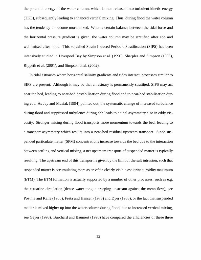
the potential energy of the water column, which is then released into turbulent kinetic energy
(TKE), subsequently leading to enhanced vertical mixing. Thus, during flood the water column
has the tendency to become more mixed. When a certain balancebetween the tidal force and
the horizontal pressure gradient is given, the water columnmay be stratified after ebb and
well-mixed after flood. This so-called Strain-Induced Periodic Stratification (SIPS) has been
intensively studied in Liverpool Bay by Simpson et al. (1990), Sharples and Simpson (1995),
Rippeth et al. (2001), and Simpson et al. (2002).
In tidal estuaries where horizontal salinity gradients andtides interact, processes similar to
SIPS are present. Although it may be that an estuary is permanently stratified, SIPS may act
near the bed, leading to near-bed destabilisation during flood and to near-bed stabilisation dur-
ing ebb. As Jay and Musiak (1994) pointed out, the systematicchange of increased turbulence
during flood and suppressed turbulence during ebb leads to a tidal asymmetry also in eddy vis-
cosity. Stronger mixing during flood transports more momentum towards the bed, leading to
a transport asymmetry which results into a near-bed residual upstream transport. Since sus-
pended particulate matter (SPM) concentrations increase towards the bed due to the interaction
between settling and vertical mixing, a net upstream transport of suspended matter is typically
resulting. The upstream end of this transport is given by thelimit of the salt intrusion, such that
suspended matter is accumulating there as an often clearly visible estuarine turbidity maximum
(ETM). The ETM formation is actually supported by a number ofother processes, such as e.g.
the estuarine circulation (dense water tongue creeping upstream against the mean flow), see
Postma and Kalle (1955), Festa and Hansen (1978) and Dyer (1988), or the fact that suspended
matter is mixed higher up into the water column during flood, due to increased vertical mixing,
see Geyer (1993). Burchard and Baumert (1998) have comparedthe efficiencies of these three
12
mechanisms with the aid of an idealised numerical model study and found that the tidal asym-
metry suggested by Jay and Musiak (1994) was the most efficient. It should be noted that a
number of other ETM mechanisms not related to density differences have been identified such
as barotropic tidal asymmetries (see e.g. Allen et al. (1980)) or topographic features such as
bends, headlands or sills (see e.g. Fischer et al. (1979)), leading at times to multiple ETMs, see
Rolinski (1999).
Postma (1954) and Zimmerman (1976) discuss in detail vertical and horizontal salinity dis-
tributions in the Marsdiep, a tidal channel connecting the western Dutch Wadden Sea with the
southern North Sea. Due to substantial fresh water supply from Lake Ijssel, high to low water
salinity differences are typically of the order of 2 psu, andthus higher than in the East and North
Frisian Wadden Sea (see figure 4). Since the vertical salinity profiles are well-mixed, Postma
(1954) concluded that gravitational circulation does not play a significant role in the Marsdiep.
The other density related potential driving mechanisms forresidual SPM transport as described
by Geyer (1993) and Jay and Musiak (1994) have not yet been discussed for the Wadden Sea.
The question which is investigated in the present work is whether the superposition of strong
tides with small horizontal density gradients as typical for the Wadden Sea (see section 2) has
the potential to generate significant net transports of suspended matter by means of the density-
related mechanisms discussed above.
13
3. Modelling tools
a. Turbulence closure model
During the last decades, two-equation turbulence closure models have proven to be most
suitable for reproducing the interaction between turbulence and mean flow in buoyancy-driven
coastal flow dynamics. These statistical models, which use one dynamic equation for the tur-
bulent kinetic energy (TKE) and one other related to the integral length scale of turbulence are
based on statistical treatment of the Navier-Stokes equations, and do thus contain a number
of empirical parameters. Those parameters have physical meanings and are thus adjustable by
means of laboratory and model (DNS, Direct Numerical Simulation) experiments. For more de-
tails of the parameter determination, see Umlauf and Burchard (2003). In the closure approach
we apply here, second-moment dynamics are reduced to algebraic relations, a simplification
which makes such closures suitable for implementation intothree-dimensional models, for de-
tails, see Burchard and Bolding (2001). In several applications, these models have proven to
agree quantitatively well with turbulence observations incoastal and limnic waters, see e.g. the
investigations by Burchard et al. (2002), Simpson et al. (2002), Stips et al. (2002), and Stips
et al. (2005).
The closure model which is applied in the present study is thek-ε model with transport
equations for the TKE,k, and the turbulence dissipation rate,ε. From k andε, the integral
length scale can be calculated by assuming equilibrium turbulence spectra. As second-moment
closure, we apply the model suggested by Cheng et al. (2002)).
The turbulence closure schemes described above have been implemented into the Public Do-
main water column model GOTM (General Ocean Turbulence Model, see http://www.gotm.net
14
and Umlauf et al. (2005)), which is used here for the one-dimensional studies described in
section b.
b. Coastal dynamics model
The dynamics of bathymetry-guided near-bed processes suchas they occur in the Wadden
Sea are best reproduced by numerical models with bottom-following coordinates. The major
advantage of such model architectures as compared to geopotential coordinates with step-like
bottom approximation is that for bottom-following flows theadvective fluxes across vertical
coordinates and thus the associated discretisation errorsare minimised (see Ezer and Mellor
(2004), Ezer (2005)). Furthermore, bottom-following coordinates allow high near-bed resolu-
tion also in domains with large depth variations (see Umlaufand Lemmin (2005)). Compared
to these advantages, the pressure gradient discretisationerror due to isopycnals crossing sloping
coordinates (see e.g. Haney (1991), Kliem and Pietrzak (1999)), an error typically associated
with bottom-following coordinates, is of minor importancefor the energetic Wadden Sea.
The three-dimensional General Estuarine Transport Model (GETM, see Burchard and Bold-
ing (2002), Burchard et al. (2004)) which has been used for the present numerical study com-
bines the advantages of bottom-following coordinates withthe turbulence module of GOTM
(see section a). A numerical feature which supports high numerical resolution computations are
high-order advection schemes, as described by Pietrzak (1998). The basic concept behind these
schemes is to apply well-tested monotone (Total Variation Diminishing, TVD) one-dimensional
methods in a directional split mode. The scheme used here is athird-order monotone ULTI-
MATE QUICKEST method, see Leonard (1991) and Pietrzak (1998) and for numerical tests,
see Burchard and Bolding (2002). The major advantage of these schemes is that they retain
15
frontal features without creating spurious oscillations and negative concentrations. Further-
more, high spatial resolution is obtained by the possibility to run GETM on parallel computers.
Simulations of scenarios with occurrence of intertidal flats are supported due to a dynamic
drying and flooding algorithm. In contrast to many other models, GETM is not explicitly shut-
ting off transports out of grid boxes in which the water depthfalls below a critical depth. Instead,
the dynamics are retained in such a way that it gradually reduces to a balance between external
pressure gradient and friction. For details, see Burchard et al. (2004).
GETM has been successfully applied to several coastal, shelf sea and limnic scenarios, see
e.g. Stanev et al. (2003b) and Stanev et al. (2003a) for turbulent flows in the Wadden Sea, Stips
et al. (2004) for dynamics in the North Sea, Burchard et al. (2005) and Burchard et al. (2007)
for studies of dense bottom currents in the Western Baltic Sea, Banas and Hickey (2005) for
estimating exchange and residence times in Willapa Bay in Washington State, and Umlauf and
Lemmin (2005) for a basin-exchange study in the Lake of Geneva.
4. One-dimensional analysis
a. One-dimensional dynamic equations
Let us consider a water column of depthH with the upwards directed coordinatez, repre-
senting the vertical structure of a water body of horizontally infinite size. An external pressure
gradient force is oscillating periodically with periodT , superimposed on a constant horizon-
tal density gradient∂xρ aligned with the direction of the external pressure gradient. With the
buoyancy
16
b = −gρ − ρ0
ρ0
(1)
and neglecting Earth’s rotation, the momentum equation is then of the form
∂tu − ∂z (νt∂zu) = −z∂xb − pg(t), (2)
where the first term on the right hand side represents the effect of the internal pressure
gradient andpg is a non-dimensional periodic external pressure gradient function with periodT
chosen such that
U(t) =1
H
∫
0
−Hu(z, t) dz = umax cos
(
2πt
T
)
, (3)
with the vertical mean velocity amplitudeumax. This construction guarantees that the ver-
tically and tidally integrated transport∫ T0
U(t) dt is zero (see Burchard (1999) for details). In
(1) g denotes the gravitational acceleration andρ0 the constant reference density, and in (2),
νt denotes the eddy diffusivity. The effect of Earth rotation can be neglected for this idealised
one-dimensional study, since the external Rossby radius ismuch larger than the dimensions of
the study area, and stratification is weak.
The transport equation for salinity is given as
∂tS + u∂xS − ∂z (ν ′
t∂zS) =S0 − S
T, (4)
where the term on the right hand side is a relaxation term. Without this term, salinity would
run away due to residual horizontal buoyancy transport. In real estuaries, this relaxation to a
certain tidal mean buoyancy is given by complex three-dimensional mixing processes which are
missing here. Thus the relaxation term can be considered as aparameterisation for these lateral
17
processes. In (4),ν ′
t denotes the eddy diffusivity. The densityρ (and thus the buoyancyb) is
then calculated by a linear equation of state, see equation (13). The horizontal salinity gradient
is prescribed, such that the buoyancy gradient∂xb (see above) can be calculated.
A simple but general suspended matter equation is given by
∂tC − ∂z (ν ′
t∂zC + wsC) = 0, (5)
with the nondimensional suspended matter concentrationC and the positive constant set-
tling velocityws. There are no fluxes of suspended matter through the bottom and the surface,
i.e. at low near-bed turbulence, suspended matter is accumulating near the bed as a kind of fluff
layer, and is mixed up into the water column when the near-bedturbulence is increasing again.
Furthermore, only low concentration non-cohesive sediments with no feedback to the buoyancy
of the flow are considered here, such that a non-dimensional view with constant settling velocity
is fully sufficient here.
As turbulence model, a two-equationk-ε model is chosen here. The TKE equation is here
of the form
∂tk − ∂z
(
νt
σk
∂zk)
= νt (∂zu)2 − ν ′
t∂zb − ε, (6)
with the TKE,k, the dimensionless turbulent Schmidt numberσk and the turbulent dissipa-
tion rateε, for which an empirical equation of a form similar to (6) is used, see e.g. Burchard
(2002). The terms on the right hand side of (6) represent shear production, buoyancy production
and dissipation.
The three potential density gradient related driving mechanisms for residual SPM transport
discussed in section c are included in this one-dimensionalmodel. Gravitational circulation is
18
included by the combination of the internal and external pressure gradient on the right hand
side of (2), SIPS is considered due to the combination of salinity advection in (4) and the
stratification effects included in the turbulence model (e.g. the buoyancy production term in
(6)) and thus included in the eddy viscosity and diffusivityin (2) and (4). Finally, the tidal
mixing asymmetry (Geyer (1993)) is included in (5) via the stratification dependence of the
eddy coefficient for SPM.
It should be noted that in this idealised case the system of hydrodynamic and turbulence
equations depends on only two non-dimensional parameters,which are the inverse Strouhal
number (see Baumert and Radach (1992))
Si =H
T umax
, (7)
and the horizontal Richardson number (see Monismith et al. (1996)),
Rx =∂xbH
2
(umax)2. (8)
An increase in depth or a decrease of tidal velocity amplitude would specifically lead to an
increasedRx, and with this, to a more pronounced tidal asymmetry.
b. One-dimensional process study
For a one-dimensional model study, we choose specificationswhich are typical for tidal
channels in the Wadden Sea: a water depth ofH = 20 m, a vertical mean velocity amplitude of
umax = 1 m s−1, a tidal period ofT = 44714 s (in accordance with the M2 constituent), and a
horizontal salinity gradient of∂xS = −1.4 · 10−4 psu m−1, such that thex-coordinate increases
in onshore direction. Salinity is relaxed to 30 psu, with a relaxation constant equal to the tidal
19
period. Sea level variations are not considered here. The simulation is initialised from some
neutral conditions (such as zero velocity, minimum turbulence, constant salinity), and is carried
out for 10 tidal periods, of which the last 5 ones turned out tobe in periodically steady state.
Results are shown for the last tidal period only. The high tide to low tide differences in salinity
(see figure 5) are about 2 psu and do thus agree well with typical winter Wadden Sea conditions,
see figure 4.
The SIPS mechanism is clearly seen in the right panel of figure5: at full flood, the surface
salinity exceeds the bottom salinity due to stronger positive salt advection near the surface.
This is an unstable state, which lasts until the end of flood. An interesting feature during ebb
is the stratification maximum during early ebb (t/T = 0.65), which is explained by the time
lag between the stratifying shear and the destratifying shear-generated vertical mixing. This has
the consequence, that the eddy viscosity is substantially smaller during full ebb than during full
flood, see the left panel in figure 6, where we show profiles shortly after full flood and full ebb
in order to allow the flow to adjust to the flow conditions. During flood the flow velocity is thus
more homogeneous in the bulk of the water column, with higherspeeds near the bottom and
lower speeds near the surface, when compared to the ebb flow (see figure 6, middle panel). This
has the consequence that near bed tidal mean flows are directed towards the coast, see figure 6,
right panel.
For SPM, two different settling velocities are considered,with values ofws = 10−3 m s−1
(fast) andws = 10−4 m s−1 (slow), respectively. The left panels of figures 7 and 8 show SPM
profiles short after full flood and short after full ebb. One can clearly see, that during flood
(due to high turbulence) the profiles are more homogeneous than during ebb, see left panels of
figures 7 and 8.
20
The tidally averaged SPM transport can be decomposed into two contributions. By intro-
ducing the tidal averaging operator
〈u〉 =1
T
∫ T
0
u dt (9)
and denoting the averages and fluctuations of velocity and SPM profiles,
u = 〈u〉, u = u − u, C = 〈C〉, C = C − C, (10)
we obtain
〈uC〉 = uC + 〈uC〉. (11)
Tidal mean SPM transport profiles〈uC〉 (see the right panels of figures 7 and 8) are directed
landwards near the bed, and seawards near the surface, with alandward oriented residual. For
the fast settling SPM, about half of this transport is due to the overlay of tidally averaged ve-
locity and SPM profiles,uC, the other 50% are due to an in average positive correlation of ebb
currents with low SPM concentrations and flood currents withhigh SPM concentrations. For
the slow settling SPM, most of the tidally averaged SPM transport is explained by an overlay of
averaged velocity and SPM profiles, except near the surface.
The tidally and vertically integrated suspended matter transport, i.e.
Cint =∫ T
0
∫
0
−HCu dzdt, (12)
is Cint = 6235 m2 for the fast sinking SPM andCint = 945 m2 for the slowly sinking SPM.
Although these are still small fractions of the total suspended matter transport which are moved
onshore and offshore during each flood and ebb tide (about 2.2% for the fast and 0.33% for
21
the slow SPM), this shows that there is a buoyancy related nettransport mechanism for a wide
range of SPM classes.
As discussed in section c, these processes are well-known for estuaries and river plumes.
However, for Wadden Sea dynamics they have so far not been considered. As shown in this
section, they may nonetheless considerably contribute to anet onshore transport of SPM also in
Wadden Sea regions.
5. Three-dimensional model studies
The tidal asymmetries in stratification and current shear are so small that it is difficult to
detect them by means of field observations. In order study thepotential effect of horizontal
density differences in a real tidal basin, we therefore apply a three-dimensional numerical model
for an idealised situation to the Sylt-Rømø Bight in the Wadden Sea area in the vicinity of the
Danish-German border. We chose this specific area, because,due to artificial dams (in the south
and north of the domain) a semi-enclosed tidal embayment with only one entrance is present, see
the right inset in figure 2. Due to these idealised conditions, many numerical model studies have
been carried out in this domain, see e.g. Dick (1987), Burchard (1998), Schneggenburger et al.
(2000), Lumborg and Windelin (2003), Lumborg and Pejrup (2005), Villarreal et al. (2005).
a. Model setup
For the three-dimensional simulations in the Sylt-Rømø-Bight, GETM (see section b) is
used in baroclinic mode. The model is forced through prescribed surface elevations at the
open boundaries in the north, west and south, see figure 9. These surface elevations have been
22
composed on the basis of harmonic analysis of the dominant M2 tide as computed by the oper-
ational model of the German Federal Maritime and Hydrographic Agency (BSH) with a period
of T = 44714 s. Other tidal constituents have not been considered in order to obtain a period
model simulation (Burchard (1995)). Freshwater flux from river run-off is specified at two loca-
tions at the eastern and north-eastern end of the Sylt-Rømø-Bight at constant rates of 10 m3s−1
for each of the two small rivers BredeA and VidaA, see figure 9. Together with a constant
precipitation rate ofP = 0.1 m per month this results in a total freshwater flux of 36 m3s−1 into
the inner Sylt-Rømø-Bight. These freshwater flux values aretypical for a winter month. The
inner Sylt-Rømø-Bight is here defined as the area composed ofbudget boxes I (south) and II
(north) as indicated in figure 9. Heat fluxes are not considered here, such that the simulation is
carried out with constant temperature. Surface momentum fluxes are also set to zero, such that
wind and surface wave effects are not considered in this idealised simulation.
The model is initialised with zero surface elevationη (however set toη = −H + hmin for
intertidal flats, whereH is the depth below zero andhmin = 0.05 m is the minimum water
depth), zero velocities and minimum values for the turbulence quantities. Salinity is initialised
with 28 psu at the mouth of the VidaA, increases linearly with distance from there to 32 psu
at a distance of 26 km, and has a constant value of 32 psu at distances larger than 26 km
from the mouth of the VidaA. SPM is initialised to unity in the entire domain after 45 tidal
periods of model spin-up. River run-off has zero salinity and SPM concentration as well as the
precipitation.
At the open boundaries, salinity is relaxed to 33 psu during inflow, with a relaxation time
scale ofτ = ∆x/un, where∆x = ∆y = 200 m is the horizontal resolution of the model grid
andun is the vertically averaged normal component of the velocityat the boundary. At the open
23
boundaries, SPM is relaxed to unity with the same time scale.Using fixed boundary values
for salt and SPM also under inflow conditions instead (equivalent to zero relaxation time scale)
would lead to the propagation of unrealistically sharp fronts into the domain.
The water column is resolved with 20 equidistantσ-layers, such that the vertical model
resolution varies between about 1.5 m at the deepest point (29.1 m) and 0.0025 m over tidal flats.
Each tidal period is resolved with104 barotropic and103 baroclinic time steps. Advection terms
for salt, momentum and SPM are discretised with the positive-definite ULTIMATE QUICKEST
scheme (see section b). For the vertical advection, a time-split scheme is additionally used in
order to guarantee numerical stability. The settling velocity of SPM is linearly reduced to zero
between the critical water depth,hcrit = 0.2 m, and the minimum water depth,hmin = 0.05 m,
in order to avoid too many iterations of the vertical advection scheme in tidal flat regions.
Two types of simulations have been carried out, one with consideration of density differ-
ences and one without. Potential densityρ is calculated from salinityS by means of the follow-
ing linear equation of state:
ρ = ρ0 + β(S − S0), (13)
where the haline expansion coefficientβ = ∂Sρ has the following values:
β =
0.78 kg m−3psu−1 for consideration of density gradients,
0 for no consideration of density gradients.
(14)
24
b. Simulation results
Both simulations, with and without consideration of density gradients were first spun up
from initial conditions for 45 tidal periods, without calculation of SPM. Between the two budget
boxes in the inner bight, a west-east section is defined, starting from the north-western tip of
the island of Sylt and cutting through the southern branch ofthe tidal channel see figure 9. At
the deepest point of this section with a water depth of 25 m, position P, time series data are
extracted.
It can be seen from figure 10 which shows time series of surfaceand bottom salinity at po-
sition P that during flood unstable and during ebb stable stratification is dominant. The salinity
amplitude at position P is about 2 psu, with values oscillating around 30 psu. This is similar
to the results of the one-dimensional simulations, see figure 5. The time series for salt at po-
sition P also shows that a quasi-periodic state was reached after 55 tidal periods, with a small
trend in salinity remaining. The latter can be explained by awater exchange time of the in-
ner Sylt-Rømø-Bight of about 265 days, which results from division of its average volume by
the freshwater fluxes and which is much longer than the duration of 45 tidal periods (about 23
days). However, the density gradients are basically in periodic state after 45 tidal periods, as
can be seen from figure 10.
Strong horizontal salinity gradients are built up in the regions of the river run-off locations
(see figure 11), specifically in the fairly narrow northern Sylt-Rømø-Bight. This is supported
by the net precipitation, which also generates very low salinities on the sandbanks south-west
of the island of Rømø.
The significant differences between ebb and flood currents are shown in figure 12 for the
area north-east of the island of Sylt. The instants of flood and ebb are defined such that for
25
ebb flow the instant of maximum current speed along the west-east section (see figure 9) is
chosen, and for flood an instant shortly after maximum flood ischosen which has a similar
maximum velocity as the maximum ebb along this section. Thisis done in order provide better
intercomparison of ebb and flood results for this section. The curved flows around the north-
eastern end of Sylt are subject to inertial effects, such that flood currents generate a lee zone
south of the north-eastern end and ebb currents generate a lee zone north of it. These tidal
asymmetries are more clearly visible in the tidal residual velocities, defined as
(ur, vr) =
∫ T
0
(U, V ) dt∫ T
0
D dt, (15)
with the vertically integrated transport vector(U, V ) and the water depthD, see figure 13.
This can also be clearly seen in figure 14 where the ebb currenthas its maximum near the
land to the west whereas the flood current maximum is deflectedfurther to the east. The fact
that ebb and flow current show different regional preferences make it impossible to evaluate
the Wadden Sea physics by only analysing point measurements. Figure 14 however shows the
significant dynamic ebb-flood differences along the considered section. During flood, strati-
fication is mostly unstable and eddy diffusivity is thus enhanced with the result that the fast
settling SPM is strongly mixed. During ebb the opposite happens: stratification is stable, eddy
diffusivity is reduced and SPM is much less mixed. Furthermore, during flood the current speed
in the upper half of the water column is much more homogeneousduring flood than during ebb.
These dynamics compare well to the one-dimensional model results shown in figures 6 and 7.
Figure 15 shows the accumulation of SPM in the budget boxes I and II of the inner Sylt-
Rømø Bight, which is done by comparing integrated SPM with total water volume in these
budget boxes. When SPM is initialised to unity after 45 tidalperiods, both values are identical.
26
During the course of 10 further tidal periods, the total SPM for the fast settling fraction is
slowly increasing in comparison to the water volume, indicating an SPM accumulation in the
inner Sylt-Rømø Bight. This is only the case for the simulation considering density gradients.
The accumulation is smaller for the northern budget box II, the volume of which is much smaller
than of the southern box I. If density gradients are neglected, an accumulation of the fast settling
SPM cannot be observed. For the slowly settling SPM, an accumulation in the inner Sylt-Rømø
Bight is not visible for the simulation considering densitygradients. For the simulation without
density gradients, SPM is even slightly washed out of the inner bight, which can be explained
by the net volume outflow due to the freshwater surplus.
Figure 16 finally shows the spatial pattern of the SPM accumulation. If density gradients are
considered, SPM is significantly accumulating in the north-eastern corner of the bight and in the
south-western part. Clear patterns of accumulation and depletion are also visible in the waters
outside the bight, probably due to non-linear interaction with the boundary conditions. When
density gradients are not dynamically considered, hardly any SPM accumulation is visible, but
some depletion is generated in the vicinity of the river run-off and on the sands due to net
precipitation.
6. Discussion
In this paper, we have shown that in general the water in the inner Wadden Sea is less
dense than the outer water, with typical tidal density amplitudes of 0.5 - 1.0 kg m−3, see figure
4. During winter, these density differences are mainly due to salinity differences, and during
summer mainly due to temperature differences, see figure 4. This is due to differential effects
27
of buoyancy fluxes (river run-off, net precipitation, surface warming), resulting in vertically
averaged densities which are smaller for shallow water thanfor deep water.
Based on this characteristic feature, we have developed thehypothesis that density differ-
ences in the Wadden Sea contribute dynamically to the net SPMaccumulation in the Wadden
Sea. As mechanisms for this, we suggest the same ones as for the Estuarine Turbidity Max-
ima which are typical for tidal estuaries, see section c. These mechanisms are based on small
differences between ebb and flood which are difficult to quantify by means of field observa-
tions. However, due to the overlay of the permanent tidal activity with the generally existing
along-current density gradients these small differences may result in long-term net onshore
SPM fluxes.
Since mass-conserving numerical models with good process resolution have the capability
to reproduce these long-term net fluxes, we rely on model simulations to challenge our hy-
pothesis. The idealised three-dimensional simulations for the Sylt-Rømø Bight do indeed show
a significant SPM accumulation in the inner bight if density gradients are considered and the
settling velocity is fast enough. Without dynamic consideration of density differences no SPM
accumulation is seen. This means that we did not find any evidence of net transport effects
of settling lag, Stokes drift and other barotropic mechanisms relying on tidal asymmetries (see
section a), although we resolve these processes with the numerical model. Other possible pro-
cesses such as scour lag and flocculation could not be quantified with our model since they are
not included in the idealised SPM dynamics resolved here.
If the settling velocity of SPM is too small, accumulation isnot seen in the model results
also when density gradients are dynamically considered. The reason for this is that SPM with a
settling velocity of onlywc = 10−4 m s−1 sinks by only about 2 m during half a tidal cycle such
28
that it is almost well-mixed (see figure 8).
The three-dimensional model results are in good agreement with the one-dimensional re-
sults. The one-dimensional model predicts for the fast settling SPM per tidal cycle a net on-
shore transport of 2.2 % of the SPM transport amplitude. The three-dimensional model predicts
about 10 % net transport during 10 tidal cycles (see figure 15), which is less than for the one-
dimensional model, but of the same order of magnitude. The differences may be explained by
the in average smaller water depth and the net outflow in the three-dimensional model. For
slowly settling SPM, the one-dimensional model predicts a net transport of 0.33 %, whereas the
three-dimensional model with dynamic density differencespredicts a zero net transport (see fig-
ure 15). Given that the net volume outflow out of the inner Sylt-Rømø Bight per tidal period is
0.1 % of the mean volume and that again the mean water depth is less for the three-dimensional
model, the SPM retention may result from a balance of a small net onshore transport and the
net volume outflow. This supported by the decrease of SPM content in the inner bight by 0.2 %
per tidal period if density differences are not considered (see figure 15).
It is not only that we see a net onshore SPM transport into the inner bight for fast settling
SPM when dynamic effects of density gradients are considered, but that we also see the mech-
anisms directly acting when studying the dynamics along a cross section leading into the inner
bight, see figure 14. During flood stratification is unstable,thus increasing turbulent mixing
with the consequence that velocity profiles are more homogeneous in the upper half of the
water column and that SPM profiles are more mixed. During ebb,the opposite is seen.
The clearest signal of SPM accumulation is seen in the northern part of the inner bight,
see figure 16. This is the location in the inner bight which is closest to an estuary: it is fairly
narrow and shallow, with substantial freshwater supply, such that significant horizontal salinity
29
gradients are resulting, see figure 11.
Of course, due to the idealised character of the simulationscarried out here (no wind, no
waves, periodic conditions, no SPM flux into sediment, no density differences due to SPM, no
flocculation) and due to fairly coarse horizontal resolution (200 m) detailed SPM dynamics on
small spatial scales cannot be reproduced. However, this numerical study strongly supports our
hypothesis that dynamic effects of density gradients in theWadden Sea significantly contribute
to SPM accumulation. This is actually not in contrast to the general assumption that the Wadden
Sea is vertically well mixed, since typical surface to bottom salinity differences are less than
0.1 psu (see figure 10).
From existing long-term observations these small verticalsalinity gradients and the resulting
small differences in ebb and flood salinity profiles cannot besignificantly detected for various
reasons. The piles installed in the Wadden Sea (see section a) are not installed in the deepest
parts of the tidal channels in order to be outside of the shipping routes. The maximum vertical
distance between salinity observations is 7.5 m for the Spiekeroog pile which according to the
numerical modelling results would amount to salinity differences of a few 1/100 psu. This is
below the absolute accuracy of the CTD sensors used here (about 0.1 psu for the high-resolution
measurements at the Spiekeroog pile) such that the discussed process cannot be assessed with
this instrumentation. Even more substantial problems are present for the observation of current
velocity profiles, where differences of about 3 % between ebband flood are typically overlaid
by barotropic ebb to flood differences as shown in figure 12.
In order to further prove our hypothesis, targeted process observations in the field and de-
tailed realistic numerical modelling studies will thus be necessary. Such observations need to
include high resolution SPM, current, density and turbulence profiling along cross-sectional
30

areas across tidal channels at various tidal phases.
With these methods it will be possible to estimate the dynamic impact of density gradients in
a number of embayments in humid and tidally dominated regions such as the Jade Bay (German
Bight), the Eastern Scheldt (The Netherlands) and the Venice Lagoon (Northern Adriatic).
Acknowledgments.
The authors greatly appreciated the support of Karsten Bolding (Asperup, Denmark) for the
maintenance of the Public Domain models GOTM and GETM.
31
References
Allen, G. P., J. C. Salomon, P. Bassoullet, Y. Du Penhoat, andC. De Grandpre, 1980: Effects of
tides on mixing and suspended sediment transport in macrotidal estuaries.Sediment. Geol.,
26, 69–90.
Andersen, T., O. Mikkelsen, A. Møller, and M. Pejrup, 2000: Deposition and mixing depths on
some European intertidal mudflats based on210Pb and137Cs activities.Cont. Shelf Res., 20,
1569–1591.
Andersen, T. and M. Pejrup, 2001: Suspended sediment transport on a temperate, microtidal
mudflat in the Danish Wadden Sea.Mar. Geol., 173, 69–85.
Banas, N. S. and B. M. Hickey, 2005: Mapping exchange and residence time in a model of
Willapa Bay, Washington, a branching, microtidal estuary.J. Geophys. Res., 110, C11 011,
doi: 10.1029/2005JC002 950.
Bartholdy, J., 2000: Processes controlling import of fine-grained sediments to tidal areas: a
simulation model.Coastal and Estuarine Environments: sedimentology, geomorphology and
geoarchaeology, Pye and Allen, Eds., Geological Society of London, London.
Baumert, H. and G. Radach, 1992: Hysteresis of turbulent kinetic energy in nonrotational tidal
flows: A model study.J. Geophys. Res., 97, 3669–3677.
Burchard, H., 1995: Turbulenzmodellierung mit Anwendungen auf thermische Deckschich-
ten im Meer und Stromungen in Wattengebieten. Ph.D. thesis, Institut fur Meereskunde,
Universitat Hamburg, published as: Report 95/E/30, GKSS Research Centre.
32
———, 1998: Presentation of a new numerical model for turbulent flow in estuaries.Hydroin-
formatics ’98, Babovic, V. and L. C. Larsen, Eds., Balkema, Rotterdam, 41–48, Proceedings
of the third International Conference on Hydroinformatics, Copenhagen, Denmark, 24-26
August 1998.
———, 1999: Recalculation of surface slopes as forcing for numerical water column models
of tidal flow. App. Math. Modelling, 23, 737–755.
———, 2002:Applied turbulence modelling in marine waters, Lecture Notes in Earth Sciences,
Vol. 100. Springer, Berlin, Heidelberg, New York, 215 pp. pp.
Burchard, H. and H. Baumert, 1998: The formation of estuarine turbidity maxima due to density
effects in the salt wedge. A hydrodynamic process study.J. Phys. Oceanogr., 28, 309–321.
Burchard, H. and K. Bolding, 2001: Comparative analysis of four second-moment turbulence
closure models for the oceanic mixed layer.J. Phys. Oceanogr., 31, 1943–1968.
———, 2002: GETM – a general estuarine transport model. Scientific documentation. Tech.
Rep. EUR 20253 EN, European Commission.
Burchard, H., K. Bolding, T. P. Rippeth, A. Stips, J. H. Simpson, and J. Sundermann, 2002:
Microstructure of turbulence in the Northern North Sea: A comparative study of observations
and model simulations.J. Sea Res., 47, 223–238.
Burchard, H., K. Bolding, and M. R. Villarreal, 2004: Three-dimensional modelling of estuarine
turbidity maxima in a tidal estuary.Ocean Dynamics, 54, 250–265.
Burchard, H., F. Janssen, K. Bolding, L. Umlauf, and H. Rennau, 2007: Model simulations of
dense bottom currents in the Western Baltic Sea.Cont. Shelf Res., submitted.
33
Burchard, H., H. Lass, V. Mohrholz, L. Umlauf, J. Sellschopp, V. Fiekas, K. Bolding, and
L. Arneborg, 2005: Dynamics of medium-intensity dense water plumes in the Arkona Sea,
Western Baltic Sea.Ocean Dynamics, 55, 391–402.
Cheng, Y., V. M. Canuto, and A. M. Howard, 2002: An improved model for the turbulent PBL.
J. Atmos. Sci., 59, 1550–1565.
De Haas, H. and D. Eisma, 1993: Suspended matter transport inthe Dollard Estuary.Neth. J.
Sea Res., 31, 37–42.
Dick, S., 1987: Gezeitenstromungen um Sylt. Numerische Untersuchungen zur halbtagigen
Hauptmondtide (M2). Dt. Hydrogr. Z., 40, 25–44.
Dronkers, J., 1986a: Tidal asymmetry and estuarine morphology. Neth. J. Sea Res., 20, 117–
131.
———, 1986b: Tide-induced residual transport of fine sediment. Physics of shallow estuaries
and bays, van de Kreeke, J., Ed., Springer, Heidelberg, Berlin, New York, 419–426.
Dyer, K. R., 1988: Fine sediment particle transport in estuaries.Physical processes in estuaries,
Dronkers, J. and J. van Leussen, Eds., Springer, Berlin, Heidelberg, New York, 295–320.
———, 1994: Estuarine sediment transport and deposition.Sediment Transport and Deposi-
tional Processes, Pye, K., Ed., Blackwell, Oxford, 193–218.
Eisma, D., 1993: Sedimentation in the Dutch-German Wadden Sea. Tech. Rep. 74, Mitteilungen
des Geologisch-Palaontologischen Instituts der Universitat Hamburg.
Ezer, T., 2005: Entrainment, diapycnal mixing and transport in three-dimensional bottom grav-
34
ity current simulations using the Mellor-Yamada turbulence scheme.Ocean Modelling, 9,
151–168.
Ezer, T. and G. L. Mellor, 2004: A generalised coordinate ocean model and a comparison of the
bottom boundary layer dynamics in terrain-following and inz-level grids.Ocean Modelling,
6, 379–403.
Festa, J. F. and D. V. Hansen, 1978: Turbidity maxima in partially mixed estuaries - A two-
dimensional numerical model.Estuarine Coastal Mar. Sci., 7, 347–359.
Fischer, H. B., E. J. List, R. C. Y. Koh, J. Imberger, and N. H. Brooks, 1979:Mixing in inland
and coastal waters. Academic Press, New York, 483 pp. pp.
Flemming, B. W. and N. Nyandwi, 1994: Land reclamation as a cause of fine-grained sediment
depletion in backbarrier tidal flats (southern North Sea).Neth. J. Aquat. Ecol., 28, 299–307.
Fofonoff, N. P. and R. C. Millard, 1983: Algorithms for the computation of fundamental prop-
erties of seawater.Unesco technical papers in marine sciences, 44, 1–53.
Geyer, W. R., 1993: The importance of suppression of turbulence by stratification on the estu-
arine turbidity maximum.Estuaries, 16, 113–125.
Groen, P., 1967: On the residual transport of suspended matter by an alternating tidal current.
Neth. J. Sea Res., 3, 564–574.
Haney, R. L., 1991: On the pressure gradient force over steeptopography in sigma coordinate
ocen models.J. Phys. Oceanogr., 21, 610–619.
Jay, D. A. and J. D. Musiak, 1994: Particle trapping in estuarine tidal flows.J. Geophys. Res.,
99, 445–461.
35
Kliem, N. and J. D. Pietrzak, 1999: On the pressure gradient error in sigma coordinate ocean
models: A comparison with a laboratory experiment.J. Geophys. Res., 104, 29 781–29 800.
Leonard, B. P., 1991: The ULTIMATE conservative differencescheme applied to unsteady
one-dimensional advection.Comput. Meth. Appl. Mech. Eng., 88, 17–74.
Lumborg, U. and M. Pejrup, 2005: Modelling of cohesive sediment transport in a tidal lagoon
an annual budget.Mar. Geol., 218, 1–16.
Lumborg, U. and A. Windelin, 2003: Hydrography and cohesivesediment modelling: applica-
tion to the Rømø Dyb tidal area.J. Mar. Sys., 38, 287–303.
Monismith, S. G., J. R. Burau, and M. Stacey, 1996: Hydrodynamic transport and mixing
processes in Suisun Bay.San Francisco Bay: the ecosystem, Hollibaugh, J. T., Ed., American
Association for the Advancement of Science, Pacific Division, San Francisco, 123–153.
Pedersen, J. B. T. and J. Bartholdy, 2006: Budgets for fine-grained sediments in the Danish
Wadden Sea.Mar. Geol., 235, 101–117.
Pejrup, M., 1988a: Flocculated suspended sediment in a micro-tidal environment.Sediment.
Geol., 57, 249–256.
———, 1988b: Suspended sediment transport across a tidal flat. Mar. Geol., 82, 187–198.
———, 1997: A fine-grained sediment budget for the Sylt-Rømø tidal basin.Helgol. Meeres-
unt., 51, 252–268.
Pietrzak, J., 1998: The use of TVD limiters for forward-in-time upstream-biased advection
schemes in ocean modeling.Mon. Weather Rev., 126, 812–830.
36
Postma, H., 1954: Hydrography of the Dutch Wadden Sea.Arch. Neerl. Zool., 10, 405–511.
———, 1961: Transport and accumulation of suspended particulate matter in the Dutch Wad-
den Sea.Neth. J. Sea Res., 1, 149–190.
———, 1981: Exchange of materials between the North Sea and the Wadden Sea.Mar. Geol.,
40, 199–213.
Postma, H. and K. Kalle, 1955: Die Entstehung von Trubungszonen im Unterlauf der Flusse,
speziell im Hinblick auf die Verhaltnisse in der Unterelbe. Dt. Hydrogr. Z., 8, 138–144.
Puls, W., H. Heinrich, and B. Mayer, 1997: Suspended particulate matter budget for the German
Bight. Mar. Pollut. Bull., 34, 398–409.
Rathlev, J., 1980: Eine einfache Salzgehaltsformel fr den praktischen Gebrauch, die der
neuesten UNESCO-Empfehlung entspricht.Dt. Hydrogr. Z., 33, 124–131.
Reuter, R., T. H. Badewien, A. Bartholomae, A. Braun, T. S. Chang, N. Gemein, M. Grunwald,
U. Harksen, A. Lubben, and J. Rullkotter, 2007: A hydrographic time-series station in the
Wadden Sea (southern North Sea).Meas. Sci. Technol., submitted.
Ridderinkhof, H., 2000: Temporal variations in concentration and transport of suspended sedi-
ments in a channel-flat system in the Ems-Dollard estuary.
Rippeth, T. P., N. Fisher, and J. H. Simpson, 2001: The semi-diurnal cycle of turbulent dissipa-
tion in the presence of tidal straining.J. Phys. Oceanogr., 31, 2458–2471.
Rolinski, S., 1999: On the dynamics of suspended matter transport in the tidal river Elbe:
Description and results of a Lagrangian model.J. Geophys. Res., 104, 26 043–26 057.
37
Schneggenburger, C., H. Gunther, and W. Rosenthal, 2000: Spectral wave modelling with non-
linear dissipation: validation and applications in a coastal tidal environment.Coast. Eng., 41,
201–235.
Sharples, J. and J. H. Simpson, 1995: Semi-diurnal and longer period stability cycles in the
Liverpool Bay region of freshwater influence.Cont. Shelf Res., 15, 295–313.
Simpson, J. H., J. Brown, J. Matthews, and G. Allen, 1990: Tidal straining, density currents,
and stirring in the control of estuarine stratification.Estuaries, 26, 1579–1590.
Simpson, J. H., H. Burchard, N. R. Fisher, and T. P. Rippeth, 2002: The semi-diurnal cycle of
dissipation in a ROFI: model-measurement comparisons.Cont. Shelf Res., 22, 1615–1628.
Stanev, E. V., B. W. Flemming, A. Bartholoma, J. V. Staneva,and J.-O. Wolff, 2007: Vertical
circulation in shallow tidal inlets and back-barrier basins.Cont. Shelf Res., in press.
Stanev, E. V., G. Floser, and J.-O. Wolff, 2003a: Dynamicalcontrol on water exchanges between
tidal basins and the open sea. A case study for the East Frisian Wadden Sea.Ocean Dynamics,
53, 146–165.
Stanev, E. V., J.-O. Wolff, H. Burchard, K. Bolding, and G. Floser, 2003b: On the circulation in
the East Frisian wadden sea: Numerical modelling and data analysis.Ocean Dynamics, 53,
27–51.
Stips, A., H. Burchard, K. Bolding, and W. Eifler, 2002: Modelling of convective turbulence
with a two-equationk-ε turbulence closure scheme.Ocean Dynamics, 52, 153–168.
Stips, A., H. Burchard, K. Bolding, H. Prandke, and A. Wuest, 2005: Measurement and sim-
38

ulation of viscous dissipation rates in the wave affected surface layer.Deep-Sea Res. II, 52,
1133–1155.
Stips, A., T. Pohlmann, K. Bolding, and H. Burchard, 2004: Simulating the temporal and spatial
dynamics of the North Sea using the new model GETM (General Estuarine Transport Model).
Ocean Dynamics, 54, 266–283.
Townend, I. and P. Whitehead, 2003: A preliminary net sediment budget for the Humber Estu-
ary.Sci. Total Environ., 314-316, 755–767.
Umlauf, L. and H. Burchard, 2003: A generic length-scale equation for geophysical turbulence
models.J. Mar. Res., 61, 235–265.
Umlauf, L., H. Burchard, and K. Bolding, 2005: General OceanTurbulence Model. Source code
documentation. Tech. Rep. 63, Baltic Sea Research Institute Warnemunde, Warnemunde,
Germany.
Umlauf, L. and U. Lemmin, 2005: Inter-basin exchange and mixing in the hypolimnion of a
large lake: the role of long internal waves.Limnol. Oceanogr., 50, 1601–1611.
van Beusekom, J., H. Fock, F. de Jong, S. Diel-Christiansen,and B. Christiansen, 2001: Wad-
den Sea specific eutrophication criteria. Tech. Rep. 14, Common Wadden Sea Secretariat,
Wilhelmshaven, Germany.
van Straaten, L. and P. Kuenen, 1958: Tidal action as a cause of clay accumulation.J. Sediment.
Petrol., 28, 406–413.
Villarreal, M. R., K. Bolding, H. Burchard, and E. Demirov, 2005: Coupling of the GOTM
turbulence module to some three-dimensional ocean models.Marine Turbulence: Theories,
39

Observations and Models, Baumert, H. Z., J. H. Simpson, and J. Sundermann, Eds., Cam-
bridge University Press, Cambridge, 225–237.
Zimmerman, J. T. F., 1976: Mixing and flushing of tidal embayments in the western Dutch
Wadden Sea. Part I: Distribution of salinity and calculation of mixing times scales.Neth. J.
Sea Res., 10, 149–191.
40

List of Figures
1 Total suspended matter in the German Bight taken by the instrument MERIS
on board of the ESA (European Space Agency) satellite ENVISAT August 12,
2003. . . . . . . . . . . . . . . . . . . . . . . . . . . . . . . . . . . . . . . . 45
2 German Bight and the positions of the measuring devices in the Wadden Sea.
The German Bight image was taken by the instrument MERIS on board of
the ESA satellite ENVISAT. The insets are taken from Google Earth satellite
scenes. On the right inset, the dams connecting the islands of Sylt and Rømø
with the mainland can be clearly seen. . . . . . . . . . . . . . . . . . . .. . . 46
3 Periods of measurement of the five piles in the German WaddenSea. The num-
bers indicate quarters of the respective years. . . . . . . . . . .. . . . . . . . 47
4 Monthly averaged salinity (top), temperature (middle) and density (bottom) dif-
ferences between high water and low for the five pile positions shown in figure
2. . . . . . . . . . . . . . . . . . . . . . . . . . . . . . . . . . . . . . . . . . 48
5 Time series of salinity during one tidal cycle in periodical steady state, simu-
lated with the one-dimensional model. Left: bottom and surface salinity; right:
bottom-surface salinity difference. The vertical full line marks slack tide after
flood, the vertical dotted lines mark the tidal phases at which the flood and ebb
profiles for figures 6 and 7 have been extracted. . . . . . . . . . . . .. . . . . 49
41

6 Profiles of viscosity and current velocity during one tidalcycle in periodical
steady state, simulated with the one-dimensional model. Left: Eddy viscosity
shortly after full flood (bold, att/T = 0.3) and shortly after full ebb (dashed, at
t/T = 0.8); middle: Absolute value of current velocity shortly afterfull flood
(bold, att/T = 0.3) and shortly after full ebb (dashed, att/T = 0.8); right:
tidal mean velocity profile, positive values represent onshore transports. . . . . 50
7 Suspended matter profiles during one tidal cycle in periodical steady state, sim-
ulated with the one-dimensional model using a settling velocity of 10−3 m s−1.
Left: Suspended matter profiles shortly after full flood (bold, att/T = 0.3) and
shortly after full ebb (dashed, att/T = 0.8); right: profile of tidal mean sus-
pended matter transport, and the contribution of a direct overlay of tidal mean
velocity and SPM profiles, as defined in equations (9) - (11). .. . . . . . . . . 51
8 Same as in figure 7, but with a settling velocity of10−4 m s−1. . . . . . . . . . 52
9 Left panel: Model topography of Sylt-Rømø Bight. The red dots show the
locations for the BredeA and the VidaA river run-off. Right panel: Areas
covered by the budget boxes I and II. The section between boxes I and II along
which simulation results will be extracted (see figure 14) isindicated as a bold
black line, the location for the salinity time series (position P, see figure 10) is
indicated as a red star. In both panels, the 0 m, 10 m and 20 m isobaths are
drawn. . . . . . . . . . . . . . . . . . . . . . . . . . . . . . . . . . . . . . . 53
42
10 Time series of salinity at position P (see figure 9) during the 55th tidal cy-
cle, simulated with the three-dimensional model under consideration of density
differences. Left: Bottom and surface salinity; right: Bottom-surface salinity
difference. . . . . . . . . . . . . . . . . . . . . . . . . . . . . . . . . . . . . 54
11 Surface salinity at high water (left panel) and low water (right panel) for the
55th tidal period for the simulation with consideration of density differences.
High and low water are defined as highest and lowest surface elevation at the
north-eastern end of the island of Sylt. The red dots indicate the locations for
the river run-off. The results are extracted from the simulation with density
effect. . . . . . . . . . . . . . . . . . . . . . . . . . . . . . . . . . . . . . . . 55
12 Vertically averaged velocity at flood (left panel) and ebb(right panel) for the
55th tidal period. (for definitions of time instants for floodand ebb, see section
b). For clarity, results are only shown for the region between the islands, and
only every 2nd arrow is shown in each direction. The results are extracted from
the simulation with density effect. . . . . . . . . . . . . . . . . . . . .. . . . 56
13 Tidal residual velocity for the 55th tidal period. For clarity, results are only
shown for the region between the islands, and only every 2nd arrow is shown in
each direction. The results are extracted from the simulation with density effect. 57
43

14 Simulation results along the cross-section indicated infigure 9 during flood and
during ebb of the 55th tidal period (for definitions of time instants for flood and
ebb, see section b). Shown are results for the current speed (upper panel), the
buoyancy frequency squared (second panel), the eddy diffusivity (third panel)
and the SPM concentration for for a settling velocity ofwc = 10−3 m s−1 (lower
panel). . . . . . . . . . . . . . . . . . . . . . . . . . . . . . . . . . . . . . . 58
15 Time series of total water volume and SPM content integrated over budget boxes
I and II for wc = 10−3 m s−1 (upper panels) and SPM flux into budget boxes
I and II and their sum forwc = 10−3 m s−1 (middle panels) and forwc =
10−4 m (lower panels) for the simulation with density differences (left panels)
and without density differences (right panels). The simulations show the tidal
periods 46 - 55, where the SPM concentration has been initialised to unity after
tidal period 45. . . . . . . . . . . . . . . . . . . . . . . . . . . . . . . . . . . 59
16 Decadal logarithm of vertically averaged SPM concentration at high water for
the simulation with consideration of density gradients (left panel) and without
density gradients (right panel) for the 55th tidal period for a settling velocity of
wc = 10−3 m s−1. The zero SPM isoline is shown in bold. High water is defined
as highest surface elevation at the north-eastern end of theisland of Sylt. The
red dots indicate the locations for the river run-off. . . . . .. . . . . . . . . . 60
44
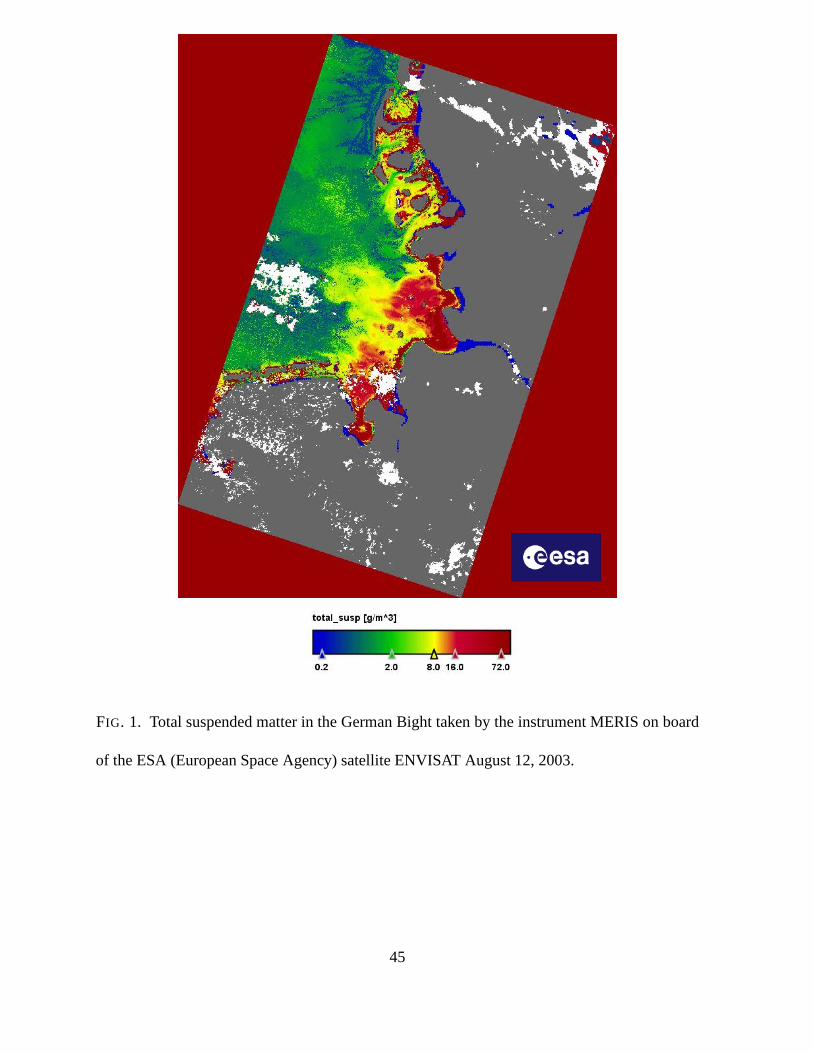
FIG. 1. Total suspended matter in the German Bight taken by the instrument MERIS on board
of the ESA (European Space Agency) satellite ENVISAT August12, 2003.
45
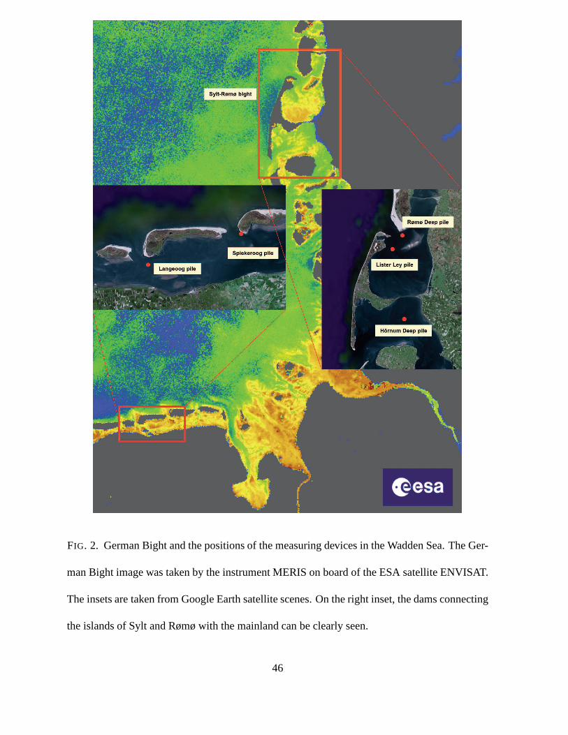
FIG. 2. German Bight and the positions of the measuring devices in the Wadden Sea. The Ger-
man Bight image was taken by the instrument MERIS on board of the ESA satellite ENVISAT.
The insets are taken from Google Earth satellite scenes. On the right inset, the dams connecting
the islands of Sylt and Rømø with the mainland can be clearly seen.
46

R¿m¿ Dyb
Lister Ley
Langeoog
H�rnum Deep
Spiekeroog
1996
1 2 3 4
1996
1 2 3 4
1997
1 2 3 4
1998
1 2 3 4
1999
1 2 3 4
2000
1 2 3 4
2001
1 2 3 4
2002
1 2 3 4
2003
1 2 3 4
2004
1 2 3 4
2005
1 2 3 4
2006
1 2 3 4
FIG. 3. Periods of measurement of the five piles in the German Wadden Sea. The numbers
indicate quarters of the respective years.
47
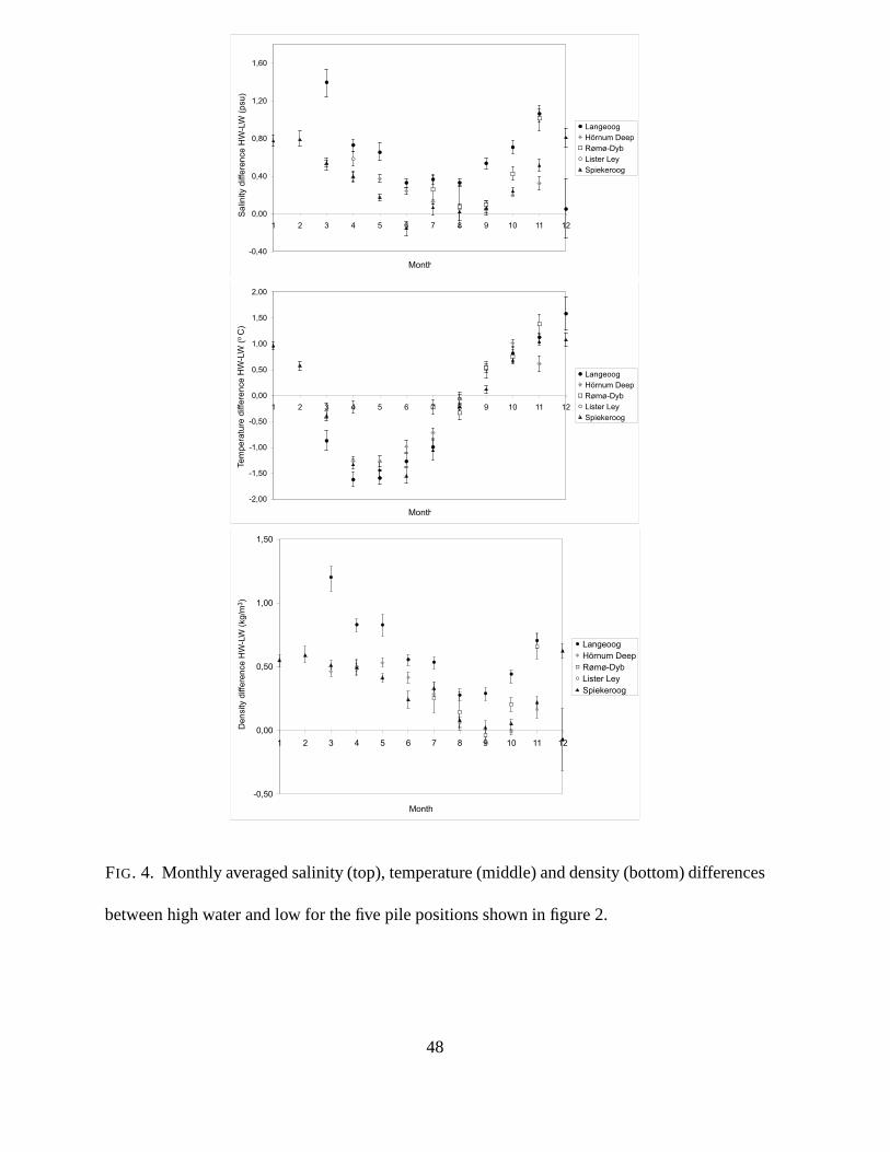
-0,40
0,00
0,40
0,80
1,20
1,60
1 2 3 4 5 6 7 8 9 10 11 12
Month
Langeoog
Hörnum Deep
Rømø-Dyb
Lister Ley
Spiekeroog
Sa
linity d
iffe
rence
HW
-LW
(p
su)
-2,00
-1,50
-1,00
-0,50
0,00
0,50
1,00
1,50
2,00
1 2 3 4 5 6 7 8 9 10 11 12
Month
Langeoog
Hörnum Deep
Rømø-Dyb
Lister Ley
Spiekeroog
Te
mp
era
ture
diffe
ren
ce
HW
-LW
(o C
)
-0,50
0,00
0,50
1,00
1,50
1 2 3 4 5 6 7 8 9 10 11 12
Month
Langeoog
Hörnum Deep
Rømø-Dyb
Lister Ley
Spiekeroog
Density d
iffe
rence H
W-L
W (
kg/m
3)
FIG. 4. Monthly averaged salinity (top), temperature (middle)and density (bottom) differences
between high water and low for the five pile positions shown infigure 2.
48
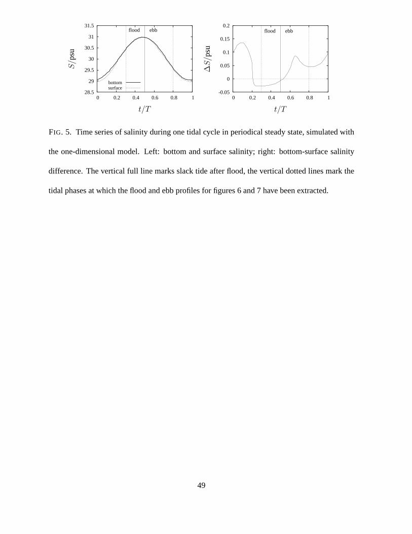
28.5
29
29.5
30
30.5
31
31.5
0 0.2 0.4 0.6 0.8 1
flood ebb
t/T
S/p
subottomsurface
-0.05
0
0.05
0.1
0.15
0.2
0 0.2 0.4 0.6 0.8 1
flood ebb
t/T
∆S/p
su
FIG. 5. Time series of salinity during one tidal cycle in periodical steady state, simulated with
the one-dimensional model. Left: bottom and surface salinity; right: bottom-surface salinity
difference. The vertical full line marks slack tide after flood, the vertical dotted lines mark the
tidal phases at which the flood and ebb profiles for figures 6 and7 have been extracted.
49
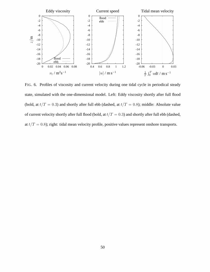
-20
-18
-16
-14
-12
-10
-8
-6
-4
-2
0
0 0.02 0.04 0.06 0.08
νt / m2s−1
z/m
Eddy viscosity
ebbflood
-20
-18
-16
-14
-12
-10
-8
-6
-4
-2
0
0.4 0.6 0.8 1 1.2
ebbflood
|u| / m s−1
Current speed
-20
-18
-16
-14
-12
-10
-8
-6
-4
-2
0
-0.06 -0.03 0 0.03
1
T
∫ T0
udt / m s−1
Tidal mean velocity
FIG. 6. Profiles of viscosity and current velocity during one tidal cycle in periodical steady
state, simulated with the one-dimensional model. Left: Eddy viscosity shortly after full flood
(bold, att/T = 0.3) and shortly after full ebb (dashed, att/T = 0.8); middle: Absolute value
of current velocity shortly after full flood (bold, att/T = 0.3) and shortly after full ebb (dashed,
at t/T = 0.8); right: tidal mean velocity profile, positive values represent onshore transports.
50
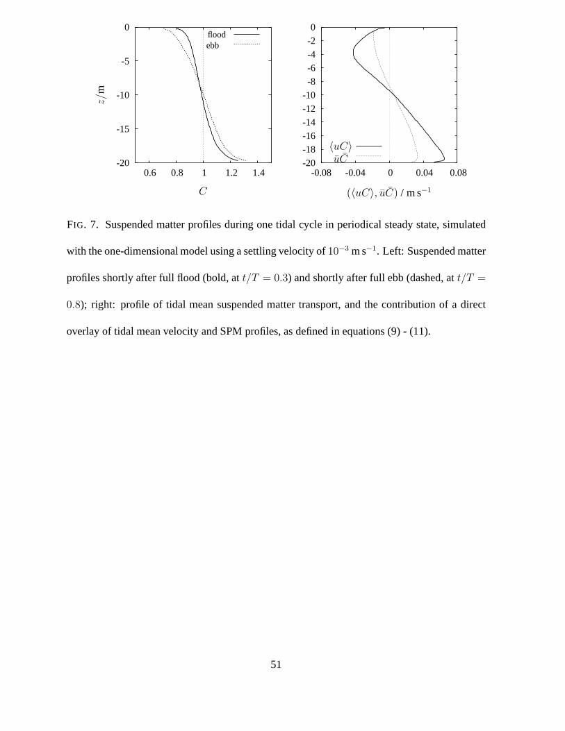
-20
-15
-10
-5
0
0.6 0.8 1 1.2 1.4
C
z/m
ebbflood
-20
-18
-16
-14
-12
-10
-8
-6
-4
-2
0
-0.08 -0.04 0 0.04 0.08
(〈uC〉, uC) / m s−1
〈uC〉uC
FIG. 7. Suspended matter profiles during one tidal cycle in periodical steady state, simulated
with the one-dimensional model using a settling velocity of10−3 m s−1. Left: Suspended matter
profiles shortly after full flood (bold, att/T = 0.3) and shortly after full ebb (dashed, att/T =
0.8); right: profile of tidal mean suspended matter transport, and the contribution of a direct
overlay of tidal mean velocity and SPM profiles, as defined in equations (9) - (11).
51
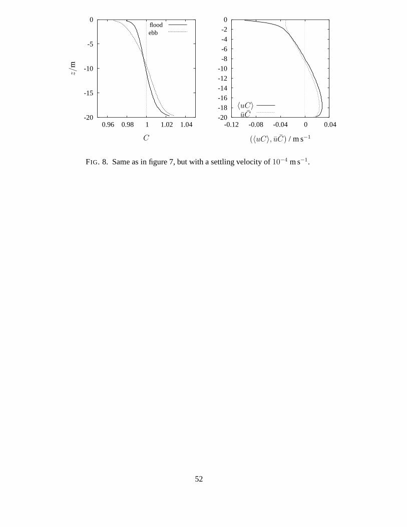
-20
-15
-10
-5
0
0.96 0.98 1 1.02 1.04
C
z/m
ebbflood
-20
-18
-16
-14
-12
-10
-8
-6
-4
-2
0
-0.12 -0.08 -0.04 0 0.04
(〈uC〉, uC) / m s−1
〈uC〉uC
FIG. 8. Same as in figure 7, but with a settling velocity of10−4 m s−1.
52
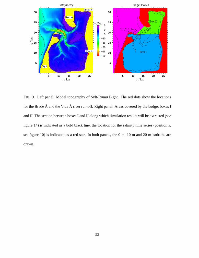
5
10
15
20
25
30
5 10 15 20 25
5
10
15
20
25
30
5 10 15 20 25
5
10
15
20
25
30
5 10 15 20 25
−30
−25
−20
−15
−10
−5
0
5
replacements
x / km
y/k
m
Bathymetry
−H/m
Sylt
Rømø
Vida A
BredeA
5
10
15
20
25
30
5 10 15 20 25
5
10
15
20
25
30
5 10 15 20 25
5
10
15
20
25
30
5 10 15 20 25
x / km
Box I
Box II
Budget Boxes
FIG. 9. Left panel: Model topography of Sylt-Rømø Bight. The reddots show the locations
for the BredeA and the VidaA river run-off. Right panel: Areas covered by the budget boxes I
and II. The section between boxes I and II along which simulation results will be extracted (see
figure 14) is indicated as a bold black line, the location for the salinity time series (position P,
see figure 10) is indicated as a red star. In both panels, the 0 m, 10 m and 20 m isobaths are
drawn.
53
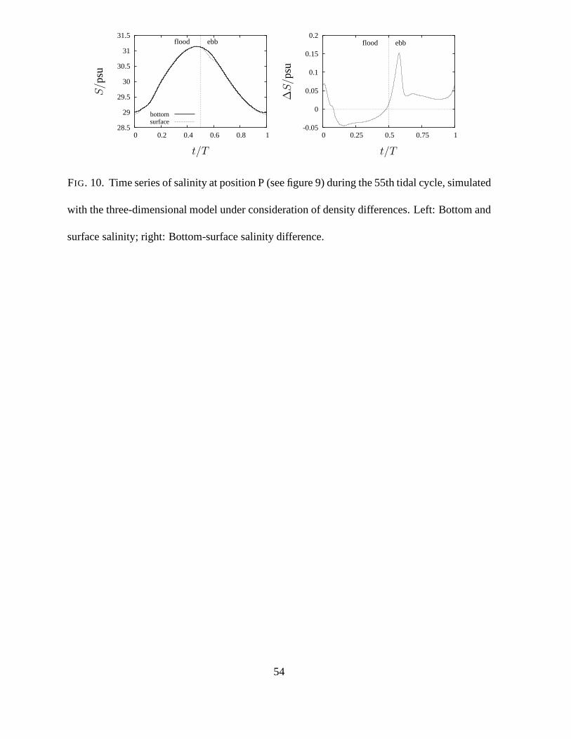
28.5
29
29.5
30
30.5
31
31.5
0 0.2 0.4 0.6 0.8 1
flood ebb
t/T
S/p
subottomsurface
-0.05
0
0.05
0.1
0.15
0.2
0 0.25 0.5 0.75 1
flood ebb
t/T
∆S/p
su
FIG. 10. Time series of salinity at position P (see figure 9) during the 55th tidal cycle, simulated
with the three-dimensional model under consideration of density differences. Left: Bottom and
surface salinity; right: Bottom-surface salinity difference.
54
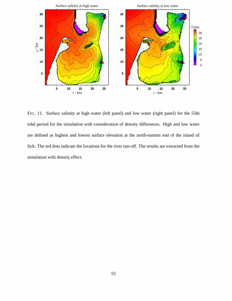
5
10
15
20
25
30
5 10 15 20 25
5
10
15
20
25
30
5 10 15 20 25
5
10
15
20
25
30
5 10 15 20 25
x / km
y/k
m
Surface salinity at high water
5
10
15
20
25
30
5 10 15 20 25
5
10
15
20
25
30
5 10 15 20 25
5
10
15
20
25
30
5 10 15 20 25
0
5
10
15
20
25
30
x / km
Surface salinity at low water
S/psu
FIG. 11. Surface salinity at high water (left panel) and low water (right panel) for the 55th
tidal period for the simulation with consideration of density differences. High and low water
are defined as highest and lowest surface elevation at the north-eastern end of the island of
Sylt. The red dots indicate the locations for the river run-off. The results are extracted from the
simulation with density effect.
55
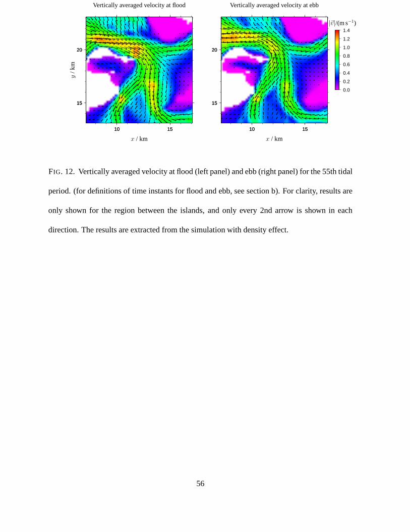
15
20
10 15
15
20
10 15
x / km
y/k
m
Vertically averaged velocity at flood
15
20
10 15
15
20
10 15
0.0
0.2
0.4
0.6
0.8
1.0
1.2
1.4
x / km
Vertically averaged velocity at ebb
|~v|/(m s−1)
FIG. 12. Vertically averaged velocity at flood (left panel) and ebb (right panel) for the 55th tidal
period. (for definitions of time instants for flood and ebb, see section b). For clarity, results are
only shown for the region between the islands, and only every2nd arrow is shown in each
direction. The results are extracted from the simulation with density effect.
56
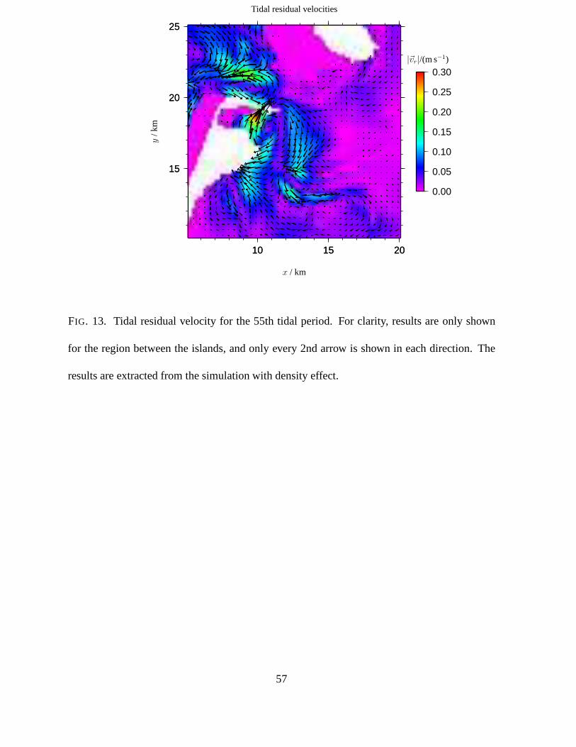
15
20
25
10 15 20
15
20
25
10 15 20
0.00
0.05
0.10
0.15
0.20
0.25
0.30
x / km
y/k
m
Tidal residual velocities
|~vr|/(m s−1)
FIG. 13. Tidal residual velocity for the 55th tidal period. For clarity, results are only shown
for the region between the islands, and only every 2nd arrow is shown in each direction. The
results are extracted from the simulation with density effect.
57
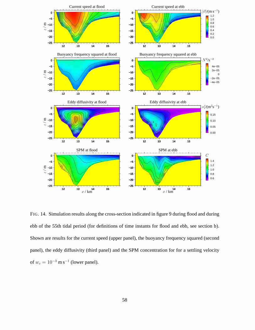
−25
−20
−15
−10
−5
0
12 13 14 15−25
−20
−15
−10
−5
0
12 13 14 15−25
−20
−15
−10
−5
0
12 13 14 15z
/m
Current speed at flood
−25
−20
−15
−10
−5
0
12 13 14 15−25
−20
−15
−10
−5
0
12 13 14 15−25
−20
−15
−10
−5
0
12 13 14 15
0.00.20.40.60.81.01.2
Current speed at ebb|~v|/(m s−1)
−25
−20
−15
−10
−5
0
12 13 14 15−25
−20
−15
−10
−5
0
12 13 14 15−25
−20
−15
−10
−5
0
12 13 14 15
z/m
Buoyancy frequency squared at flood
−25
−20
−15
−10
−5
0
12 13 14 15−25
−20
−15
−10
−5
0
12 13 14 15−25
−20
−15
−10
−5
0
12 13 14 15
−4e−05
−2e−05
0
2e−05
4e−05
Buoyancy frequency squared at ebb
N2/s−2
−25
−20
−15
−10
−5
0
12 13 14 15−25
−20
−15
−10
−5
0
12 13 14 15−25
−20
−15
−10
−5
0
12 13 14 15
z/m
Eddy diffusivity at flood
−25
−20
−15
−10
−5
0
12 13 14 15−25
−20
−15
−10
−5
0
12 13 14 15−25
−20
−15
−10
−5
0
12 13 14 15
0.00
0.05
0.10
0.15
Eddy diffusivity at ebbν ′
t/(m2s−1)
−25
−20
−15
−10
−5
0
12 13 14 15−25
−20
−15
−10
−5
0
12 13 14 15−25
−20
−15
−10
−5
0
12 13 14 15x / km
z/m
SPM at flood
−25
−20
−15
−10
−5
0
12 13 14 15−25
−20
−15
−10
−5
0
12 13 14 15−25
−20
−15
−10
−5
0
12 13 14 15
0.6
0.8
1.0
1.2
1.4
x / km
SPM at ebbC
FIG. 14. Simulation results along the cross-section indicatedin figure 9 during flood and during
ebb of the 55th tidal period (for definitions of time instantsfor flood and ebb, see section b).
Shown are results for the current speed (upper panel), the buoyancy frequency squared (second
panel), the eddy diffusivity (third panel) and the SPM concentration for for a settling velocity
of wc = 10−3 m s−1 (lower panel).
58
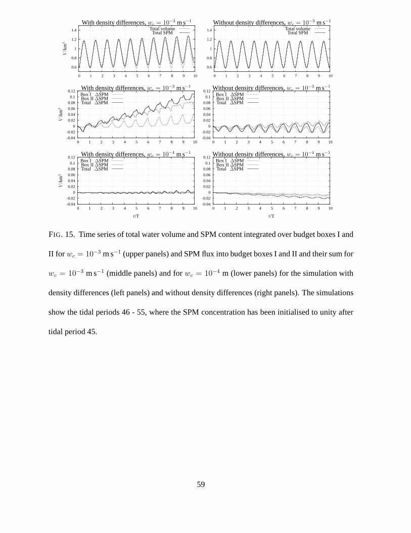
0.6
0.8
1
1.2
1.4
0 1 2 3 4 5 6 7 8 9 10
V/k
m3
With density differences,wc = 10−3 m s−1
Total volumeTotal SPM
0.6
0.8
1
1.2
1.4
0 1 2 3 4 5 6 7 8 9 10
Total volumeTotal SPM
Without density differences,wc = 10−3 m s−1
-0.04
-0.02
0
0.02
0.04
0.06
0.08
0.1
0.12
0 1 2 3 4 5 6 7 8 9 10
With density differences,wc = 10−3 m s−1
V/k
m3
Box I ∆SPMBox II ∆SPMTotal ∆SPM
-0.04
-0.02
0
0.02
0.04
0.06
0.08
0.1
0.12
0 1 2 3 4 5 6 7 8 9 10
Box I ∆SPMBox II ∆SPMTotal ∆SPM
Without density differences,wc = 10−3 m s−1
-0.04
-0.02
0
0.02
0.04
0.06
0.08
0.1
0.12
0 1 2 3 4 5 6 7 8 9 10
Box I ∆SPMBox II ∆SPMTotal ∆SPM
V/k
m3
t/T
With density differences,wc = 10−4 m s−1
-0.04
-0.02
0
0.02
0.04
0.06
0.08
0.1
0.12
0 1 2 3 4 5 6 7 8 9 10
Box I ∆SPMBox II ∆SPMTotal ∆SPM
t/T
Without density differences,wc = 10−4 m s−1
FIG. 15. Time series of total water volume and SPM content integrated over budget boxes I and
II for wc = 10−3 m s−1 (upper panels) and SPM flux into budget boxes I and II and theirsum for
wc = 10−3 m s−1 (middle panels) and forwc = 10−4 m (lower panels) for the simulation with
density differences (left panels) and without density differences (right panels). The simulations
show the tidal periods 46 - 55, where the SPM concentration has been initialised to unity after
tidal period 45.
59
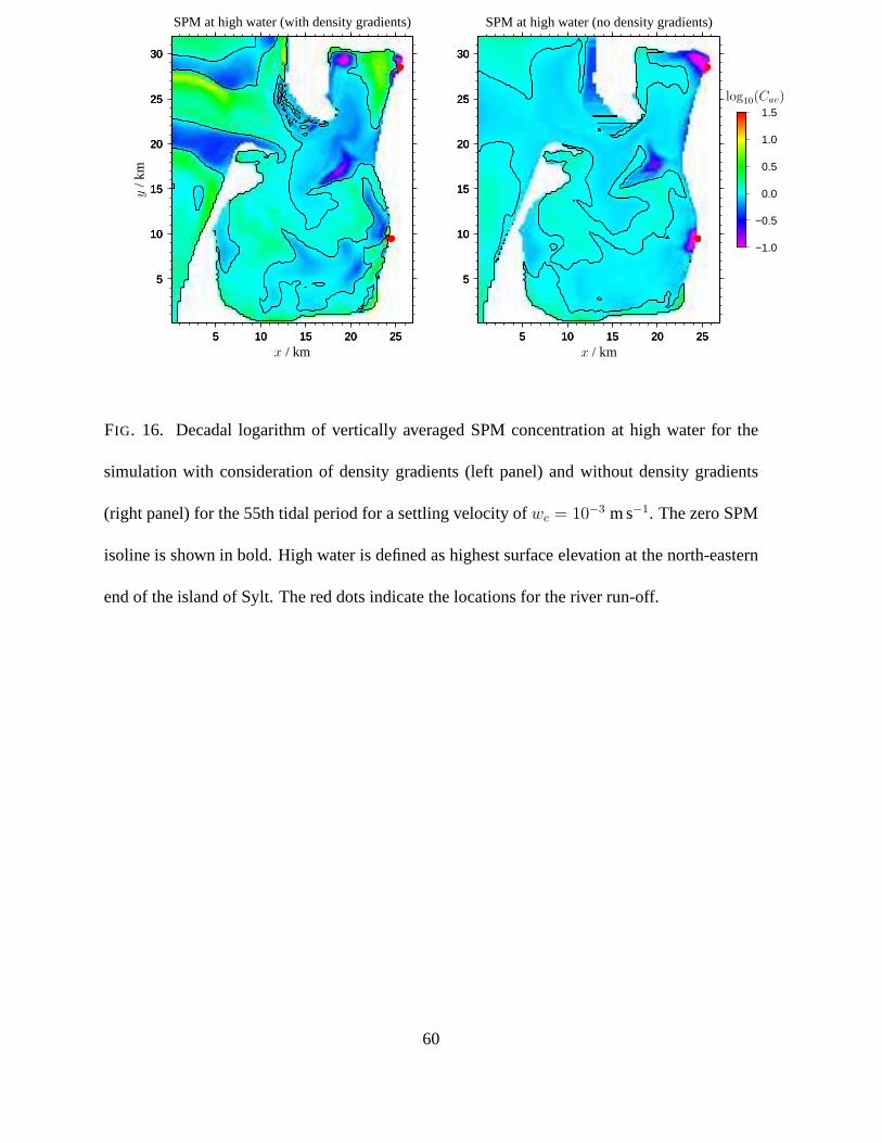
5
10
15
20
25
30
5 10 15 20 25
5
10
15
20
25
30
5 10 15 20 25
5
10
15
20
25
30
5 10 15 20 25
x / km
y/k
m
SPM at high water (with density gradients)
5
10
15
20
25
30
5 10 15 20 25
5
10
15
20
25
30
5 10 15 20 25
5
10
15
20
25
30
5 10 15 20 25
−1.0
−0.5
0.0
0.5
1.0
1.5
x / km
SPM at high water (no density gradients)
log10(Cav)
FIG. 16. Decadal logarithm of vertically averaged SPM concentration at high water for the
simulation with consideration of density gradients (left panel) and without density gradients
(right panel) for the 55th tidal period for a settling velocity of wc = 10−3 m s−1. The zero SPM
isoline is shown in bold. High water is defined as highest surface elevation at the north-eastern
end of the island of Sylt. The red dots indicate the locationsfor the river run-off.
60

List of Tables
1 Instrument specifications of the GKSS (Langeoog, Rømø Deep, Lister Ley, Ho-
ernum Deep) and the University of Oldenburg (Spiekeroog) pile stations. . . . 62
61
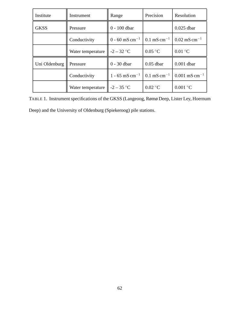
Institute Instrument Range Precision Resolution
GKSS Pressure 0 - 100 dbar 0.025 dbar
Conductivity 0 - 60 mS cm−1 0.1 mS cm−1 0.02 mS cm−1
Water temperature -2 – 32◦C 0.05◦C 0.01◦C
Uni Oldenburg Pressure 0 - 30 dbar 0.05 dbar 0.001 dbar
Conductivity 1 - 65 mS cm−1 0.1 mS cm−1 0.001 mS cm−1
Water temperature -2 – 35◦C 0.02◦C 0.001◦C
TABLE 1. Instrument specifications of the GKSS (Langeoog, Rømø Deep, Lister Ley, Hoernum
Deep) and the University of Oldenburg (Spiekeroog) pile stations.
62