impact of export horticulture farming on...

International Journal of Food and Agricultural Economics

ISSN 2147-8988, E-ISSN: 2149-3766

Vol. 3 No. 4, 2015, pp. 65-81

65

IMPACT OF EXPORT HORTICULTURE FARMING ON PER

CAPITA CALORIE INTAKE OF SMALLHOLDER FARMERS IN

EASTERN AND CENTRAL PROVINCES IN KENYA

Jane Wambui Chege

University of Nairobi, Department of Agricultural Economics

P.O Box 29053-00625, Nairobi, Kenya, Email: [email protected]

Rose Athiambo Nyikal

University of Nairobi, Kenya

John Mburu

University of Nairobi, Kenya

Beatrice Wambui Muriithi International Centre for Insect Physiology and Ecology (ICIPE), Nairobi, Kenya

Abstract

In attempting to achieve household food security for smallholder farmers, synergies and

tradeoffs exist between cash cropping, food cropping and food security. Available evidence

on the impact of cash cropping on food security shows mixed results. The objective of this

paper was to assess the impact of export horticulture farming on food security of smallholder

farmers in Kenya in two provinces in different agro-ecological zones with different resource

and infrastructural endowments, crop growing and marketing conditions. This was done

using propensity score matching. The results indicate a positive impact on food security in

high potential area and a negative impact in the arid area that is already food deficit.

Encouraging export horticulture or cash cropping, aiming at achieving household food

security, may not be a one size fit all. Regional differences and particular growing and

marketing conditions as well as intra household income distribution patterns play a role and

should be considered.

Key words; Export horticulture; food security, per capita calorie intake; smallholder

farmers; impact; propensity score matching.

1. Introduction

Horticultural production for export is a major cash cropping practice among small holder

farmers in Central, Eastern and Rift Valley provinces in Kenya. This study assessed the

impact of this practice on the food intake of horticultural farmers in Eastern and Central

provinces. The two areas of study are different in terms of agro ecological endowment

environment and infrastructural development. The article proceeds as follows: section one

provides a background of the practice in Kenya and introduces the research problem and

objectives of the study, section two describes the methods of analysis in terms of how food

intake was calculated and gives a brief description of sampling and data collection

procedures followed and the empirical model employed. The results and discussions are

presented in section three, while section four provides the conclusion and the policy

recommendations.

Impact Of Export Horticulture Farming On Per Capita Calorie…

66

1.1. Background

Commercialization of agriculture, comprising of a shift from food production for home

consumption to production for the market, is often stipulated as the way out of poverty and a

means to enhance food security (Kennedy & Cogill, 1987). One particular manifestation of

commercialization is cash cropping. Whilst commercialization can include market oriented

production of staple food crops, cash cropping involves crops produced for cash that have a

higher value than those consumed within the household and tends to require a greater degree

of specialization.

Horticultural production for export is a major cash cropping practice in Kenya and is

ranked third in terms of foreign exchange earnings after tourism and tea (HCDA, 2009). It

contributes 30 percent of agricultural GDP and continues to grow at between 15 and 20

percent per year (GoK, 2012). Kenya has been the most successful exporter of horticultural

products in the sub-Saharan Africa. The European Union (EU) is the dominant market for

Kenyan exports and after Morocco Kenya is the biggest fresh vegetable supplier to the EU

(Legge, Orchard, Graffham, Greenhalgh and Kleih. 2006). The horticultural export sector in

Kenya is characterized by participation of smallholder farmers faced by numerous technical

and institutional challenges that majorly stem from stringent market regulations (Asfaw,

Mithöfer, & Waibel, 2007). In the 1990s, researchers estimated that three quarters of fresh

fruit and vegetable exports production came from smallholder growers. However,

participation of smallholders has declined in recent years due to the high cost of managing

smallholder out growers in the face of new food-safety and quality regulations such as

GlobalGAP standards and the need to have a critical size and number (Legge et al. 2006).

Nevertheless, McCulloch and Ota (2002), report that smallholders participating in export

horticulture, whether as producers or the workforce employed in the sector, are better off

than non-participating smallholders, with average annual household incomes of the former

being higher.

Though the export horticulture sector has been a success in terms of foreign exchange

earnings, its impact on smallholder household food security remains under investigated.

Available evidence on the effect of cash cropping systems on food security shows mixed

results. Different negative and positive impacts can be identified and vary with choice of

cash crops and the situation in which they are being grown and marketed. Cash cropping is

associated with increased staple food production due to the synergy between the two systems

(Bolwig & Odeke, 2007; Govereh &Jayne, 1999; Von Braun & Kennedy, 1986). On the

other hand, Anouk (2010) and Sorre (2011) indicate that cash cropping often increases the

competition for resources between cash and food crops, thus posing a threat to food security.

Langat et al. (2012), point to the deteriorating food security situation of tea farmers in Nandi

Kenya and conclude that food security is not guaranteed by higher cash crop production and

consequently recommend diversification of farm enterprises. An extensive review of studies

on the impact of export driven cash crops on smallholder households by Schneider and

Gugerty (2010) conclude that given the heterogeneity of crops and production structures

across the African continent, drawing strong policy conclusions from the available evidence

may not be right. The authors further observe that the empirical data available to evaluate the

impact of cash crop production on smallholder welfare remains relatively weak.

Policies promoting export horticulture assume that realization of increased household

incomes through cultivation of export oriented cash crops would guarantee improved

household food security. However this market niche is surrounded by a myriad of non-

uniform growing, marketing and intra-household conditions whose challenges and outcomes

or effects are neither automatic nor uniform. Empirical findings are necessary to back policy

interventions in order to ensure positive outcomes are reinforced and bottlenecks addressed.

The information generated by the current study will assist policy makers in designing

J. W. Chege, R. A. Nyikal, J. I. Mburu and B. W. Muriithi

67

horticultural production and export policies that ensure positive effects are enhanced while

any negative impacts are minimized or entirely eliminated and farmers’ welfare improved.

1.2. Conceptual Framework

Sen’s (1981) entitlement theory outlines the different ways in which individuals can

acquire food: a) production based entitlements i.e. through own food production; b) trade

based entitlements that is through exchange of cash crops or physical assets; c) own labour

entitlements through sale of labour power for wage; and, d) inheritance, and transfer

entitlement which refer to informal gifts from individuals and formal gifts from government.

The level and the mix of these entitlements depend on a households resource endowments

including human capital, type of market integration for agricultural produce, food and labour.

Effect on these variables, ultimately affect food intake.

Following this theory, the current study conceptualizes the food security status as an

outcome of household/farmer social economic characteristic and non-controllable external

environmental factors. The same factors also affect a farmer’s decision to grow export

horticulture or not to grow as shown in Figure 1. This decision affects the farmer’s resource

allocation decision, either to produce horticultural crops for export market, food crop and or

engage in off farm employment or a level of mix among all these alternatives. Households

that choose to grow export horticulture may undergo a transition from food crop farming for

sale to domestic consumers and own consumption, to production for export market, implying

a shift of resource allocation. The ultimate effect of a particular cash crop on food security or

food intake will then be an outcome of different factors and specific household decisions

hence complex interactions arise. This then becomes an empirical issue since the possible

effects and interactions are not straightforward and vary from crop to crop as well as the

prevailing growing, marketing and household conditions. There is consensus that cash

cropping would increase income of smallholder farmers, though the variance of this income

is high. However, effect of this increased income would vary from one household to another

depending on household specific characteristics and the external environment as shown

Figure 1.

Generally, households will result to reduced food intake if the price of the export crop is

lower relative to the prevailing food prices. Market concentration in this case plays a vital

role. Where markets are concentrated i.e. there are fewer buyers compared to a large number

of smallholder farmer sellers, the prices may be low due to reduced bargaining power of the

farmers. Price fluctuations in the global market increase variability of income. Consumer

demand for high quality vegetables abroad means that export vegetables that fall short of the

specifications are rejected or bought at very low prices. In cases where production of export

horticulture results to a shift of productive resources from food crop production to production

of export vegetables, production of food crop reduces. Consequently, if income realized from

sale of the export crops, (depending on the decisions of the person in control) is not spent on

purchasing food items, this reduce food available for household consumption. Research has

shown that if women are in control of income, they tend to spend more on food consumption

related expenditures. In contrast men are more inclined to non-food expenditures such as

education and purchase of durable assets. On the other hand, if increased income from export

horticulture is spent on increasing food crop production and or purchase of food products for

the household then this will result into increased food intake. In addition, if production of

export horticulture does not necessarily translate to shift of production resources away from

food crop production, then the level of food intake could not be negative. The different

interactions are illustrated in Figure 1.


68

Figure 1. Conceptual framework of the linkages between horticultural export production and

food security

2. Methods of Analysis

2.1 Measuring Food Security

Food security is a situation that exists when all people, at all times, have physical, social

and economic access to sufficient, safe and nutritious food that meets their dietary needs and

food preferences for an active and healthy life (Bongaarts, 2007). This definition integrates

distinct but inter-related dimensions of the concept of food security, that is; access to food,

availability of food, the biological utilization of food, as well as the stability of all these

factors. Due to its nature and complexity, there are approximately 200 definitions and 450

indicators of food security (Hoddinott, 1999). Like the concepts of health or social welfare,

there is no single, direct measure of food security that can effectively capture the multiple

dimensions to the problem (Bongaarts, 2007; Riely, Mock, Cogill, Bailey & Kenefick,

Farmer specific characteristic and

Endowments levels; Human, Physical

and social capital

Decision to grow

Export cash crop

Decision not to grow

Export cash crop

Prevailing external environment; Market prices, physical

infrastructure, political environment, agro ecological conditions,

climate, food safety standards arrangements, technology, macro and

trade policies, market concentration

Income and food

supply from

subsistence crops and

Crops for the domestic

markets, participation

in labour markets

Level of Food intake

Income from cash crops

Reduced food intake;

-Reduced export crop

price and High food

prices, low productivity

of food crops; use of

income for non-food

expenditures,

Increased food intake;

-High export crop prices,

high productivity of food

crops, Use of income to

purchase food

Food security

Other dimensions of food security; Stability, Utilization and Access


69

(1999); Webb et al. 2006). There is no any form of a consensus on the core household food

security indicators that are needed in order to properly measure and monitor food security

around the world (Carletto, Zezza and Banerjee, 2013) However, the field is rapidly growing

and undergoing constant development towards a gold standard of monitoring hunger

worldwide. The United States Department of Agriculture (USDA) Household Food

Insecurity Access Scale and Food Insecurity Experience Scale (FIES) for example have been

shown to be a stable, robust, and reliable food access measurement tools. USDA scale

consists of 18 core-module questions, which work systematically together to provide a

measurement tool for identifying, with considerable sensitivity, the level of severity of food

insecurity/hunger experienced in a household.

However, in practice, a variety of indicators are used for food security analysis (Carletto

et al. 2013). These indicators though, cannot measure the different dimensions of food

security hence composite measures are preferred. In fact, due to multidimensionality of the

concept, FAO has a suite of indicators variables for different dimensions, which together

give an indication of the level of food security and are useful in building composite indices

(Santeramo, 2015).

However, that notwithstanding, the current study have employed per capita calorie intake

a measure of food availability as a partial indicator of food security. Per capita calorie intake

is relevant in calculating the Average Dietary Energy Supply Adequacy (ADESA) an

indicator of food availability under FAOSTAT. ADESA expresses the dietary energy supply

as a percentage of the Average Dietary Energy Requirement. Comparably, per capita calorie

intake employed in this study compares the per capita energy consumption in Kcal and

compares it with the average dietary energy requirement in Kenya. Households are then

termed as either food secure or food insecure depending on whether the energy consumption

is more or less than the average dietary energy requirement. This principle is employed by

FAO undernourishment measure used to report on the state of food security worldwide by

capturing the average availability of food against requirements at the national level.

Per capita calorie intake was estimated using 7 day recall method where household total

energy consumption was calculated (Swindale & Bilinsky, 2006). Using the formulae;

ii

n

ii BWC 1 (1)

Where;

Ci is the household total calorie intake estimate, Wi is the weight in grams of intake of

food commodity i, and Bi is the standardized food energy content of the ith

food

commodity (from nutrient conversion tables).

Ci was then divided by household size to get per capita calorie intake (PCI), and then

compared to 2250 kilocalories average energy requirement as the threshold.

2.2. Study Area

The study was carried out between 2010 and 2011 in two districts of the major export

vegetable producing provinces in Kenya (Mbooni district of Eastern province and Kirinyaga

district of Central province). These two districts represent the highest number of smallholder

farmers producing vegetables for export market in the two provinces respectively. It is

important to note here that Mbooni district has since became a sub county within Makueni

County from Eastern Province after the revision of administrative boundaries in Kenya in the

year 2013, while Kirinyaga district is a county from the Central Province. However for the

purpose of this study, these study areas are referred to as districts as they were when the

research was undertaken. The two provinces are different in both natural climatic conditions


70

/agro-ecological zone and in infrastructural development and were selected to facilitate

comparison of the impacts in different settings.

Mbooni district lies within the arid and semiarid zones of the country. It is a low-lying

district rising from 700 meters above sea level at the lowlands to 1900 meters above sea

level. With a population of 177,832 persons, the district covers an area of square kilometer

894.6 and has very high poverty level with absolute poverty standing at 64.3 percent

(MPND, 2008a). The province’s road and irrigation infrastructure is underdeveloped

compared to Central Province. Kirinyaga district is one of the six districts in Central

Province that lies in the high potential areas of the country and has a well-developed

irrigation and road network. The district covers an area of square kilometer 1,437 and has a

population of 528,054 persons. Kirinyaga District has absolute poverty of 36 percent. The

district lies between 1150 to 5380 meters above sea level. It receives two rainy seasons, the

long and the short rains between March to May and October to November respectively

(MPND, 2008b).

2.3. Study Context, Data and Sampling Procedures

The study forms part of a larger project –Drivers, Viability and Livelihood Impacts of

Compliance with private food safety standards in Kenya (DriVLIC Kenya), funded by

International Development Research Centre (IDRC) undertaken by the University of Nairobi

in collaboration with the Fresh Produce Exporters Association of Kenya and the Ministry of

Agriculture in Kenya. The sampling unit in this study was a household, comprising of people

living together headed by one person and having one cooking arrangement. Data used in this

study was collected using structured questionnaire in two phases; the baseline data

containing farmer socio-economic characteristics and production information was collected

between July and October 2010, while the consumption and household characteristics data

was collected between August and November year 2011. The list of farmers from an initial

baseline survey of the DriVLIC Kenya project formed the sampling frame for the second

phase. The sampling frame was used to generate seven categories of farmers based on their

compliance status with Global GAP. Individually fully compliant farmers who are growers

of exporters, Group contract farmers (who own facilities, production process and keep their

own records), Group scheme farmers (exporters own facilities, keeps records and controls

production), non-compliant farmers who abandoned standards after adopting, non-compliant

farmers who have never adopted standards and finally farmers who do not grow export

vegetables. From the sampling frame, a total of 372 households, (228 in Kirinyaga and 144

in Mbooni) were selected using proportionate to population size selection of the follow-up

survey. These were later collapsed to two groups of growers and non-growers for the purpose

of this study.

2.4. Propensity Score Matching Theory

The impact of participation in production of horticulture for export market on food intake

is given by the difference in the food intake when a household participates in export

horticulture production and the food intake when the same household does not participate;

that is, the food intake outcome with and without treatment. Clearly, we cannot have both

outcomes for the same household at the same time. Hence, one has to develop a proxy for the

missing data or counterfactual as referred to in impact assessment literature. Taking the mean

outcome of nonparticipants as an approximation of the counterfactual is not advisable, since

participants and non-participants usually differ even in the absence of treatment. This

problem is known as selection bias (Caliendo & Kopeinig, 2008).


71

The basic idea in propensity score matching method is to find in a large group of non-

participants, households who are similar to those participating in all relevant pretreatment

characteristics X. Once this is achieved, differences in outcomes of this well selected and

thus adequate control group (non-participants) and of treatment group (participants) can be

attributed to the participation in export horticulture farming. Since conditioning on all

relevant covariates is limited in the case of a high dimensional vector X, we use balancing

score b(X) which is a function of the relevant observed covariates X such that the conditional

distribution of X given b(X) is independent of the assignment into treatment. This balancing

score is the propensity score i.e. (the probability of participating in export horticultural

farming given the observed characteristic X). Given by,

b(X) =Pr (Z=1/X) (2)

Where Z denotes the participation status in production for the export market, and 1

denotes a household participates and 0 otherwise. X is the multidimensional vector of

pretreatment characteristics.

The propensity score is a function such that the conditional distribution of X given b(X) is

the same in both groups. Given that the propensity score is a balancing score, the probability

of participation conditional on X will be balanced such that the distribution of observables X

will be the same for participants and non-participants. Consequently, the differences between

both groups are reduced to the only attribute of treatment assignment and unbiased impact

estimates can be produced (Rosenbaum & Rubin, 1983). Propensity scores are estimated

using choice models either probit or logit model which yield similar results.

An estimate of the propensity score is not enough to estimate the ATT. The reason is that

the probability of observing two units with exactly the same value of the propensity score is

in principle zero since b(X) is a continuous variable. Various methods (matching procedures)

have been proposed in the literature to overcome this problem. Matching procedures based

on this balancing score are known as propensity score matching (PSM). Three of the most

widely used are Nearest Neighbor Matching (NNM), Radius Matching (RM) and Kernel

Based Matching (KBM). All matching procedures contrast the outcome of a treated

individual with outcomes of comparison group members. ATT can be noted as;

E[Y 1|D = 1] − E[Y 0D = 0] = ATT + E[Y 0|D = 1] − E[Y 0D = 0 (3)

The difference between the left hand side of the equation and ATT is the so called

‘selection bias’. The true parameter ATT is only identified if, (Caliendo & Kopeinig, 2008)

E[Y 0|D = 1] - E[Y 0D = 0] =0 (4)

In non-experimental studies, one has to invoke some identifying assumptions when using

propensity score matching to solve the selection problem namely -Unconfoundedness or

conditional independence assumption (CIA), and the Common Support Condition (CSC).

Conditional independence assumption indicates that the selection is exclusively based on the

vector of observables X that determines the propensity score and that treatment is random

and uncorrelated with the outcome once controlled for X (Caliendo & Kopeinig, 2008;

Rosenbaum & Rubin, 1983). Sensitivity analysis a test of fulfillment of conditional

independence assumption examines how strong the influence of unobservable characteristics

on the participation process needs to be, in order to attenuate the impact of participation on

potential outcomes.

In order to ensure randomized selection the common support condition needs to be

applied which guarantees individuals with identical observable characteristics a positive


72

probability to belong both to the treatment and controls groups. ATT is only defined within

the region of common support. This is because only in the overlapping subset of the

comparison group and treatment group comparable observations can be matched. A violation

of the CSC is a major source of bias due to comparing incomparable individuals (Heckman,

Ichumura, & Todd 1997). Given that CIA holds and assuming additionally that there is

overlap between both groups, the PSM estimator for ATT can be written in general as

ATT = E {E {Y1|Di = 1, p (Xi)} − E {Y0|Di = 0, p (Xi)} |Di = 1} (5)

Where ATT is the average treatment effect on the treated conditioned on participation, Y1

denote the food security outcome for an individual if the person is a participant, Y0 the food

security outcome if the person is nonparticipant. In a regression framework, the treatment

effects model is given by

Y= a+ β bi + c Xi +ei (6)

Where Y is the household food intake level as measured by per capita calorie intake, bi is the

propensity score, of the ith

farmer, Xi is a vector of control variables such as farmer/

household characteristics, and β measures the impact of participation on food intake.

Table 1. Summary Statistics of Smallholder Farmers in Kirinyaga and Mbooni

Variable code

Kirinyaga

N=241

Mbooni

N=140

Variable description Mean SD Mean SD

HHGENDER Gender of household head(1=Male 0

Female)

0.82 0.38 0.79 0.41

HHSIZE Size of the household 3.91 1.73 5.79 2.2

HHEDUC Years of education of the household

head

8.26 3.92 7.95 4.26

GROUPMEMBER Whether the household head belong to

a group (1= Yes, 0 = Otherwise)

0.64 0.48 0.45 0.50

HHOCCUPATION The primary occupation of the

household head

0.85 0.36 0.70 0.45

HHFARMEXPR Number of years of farming 20.54 13.25 20.4 12.35

TOTLABOURERS Family & hired labourers 3.90 2.40 3.38 1.62

FAMLABOURERS Number of family labourers 1.84 0.87 2.10 1.17

OWNLAND Land area owned by the household 0.53 1.29 0.50 0.77

AGRICLAND Land area under cultivation 2.48 1.67 1.65 1.02

HHAGE Age of the household head 49.92 13.52 48.52 13.93

LVSTKUNITS Number of livestock equivalent 2.99 1.80 3.21 1.86

DISTMARKET Distance in Km to the nearest market 3.37 2.87 6.10 5.00

DISTINPUT Distance to the nearest input shop (

walking hours)

1.14 0.96 1.43 0.93

DISTWATER Distance in Km to the nearest water

source

0.32 0.87 0.62 1.73

TOTACRES Total acres of land owned plus rented 2.92 2.38 2.53 1.68

EXPVEGAREA Land area under export vegetables 0.53 0.54 0.24 0.13


73

3. Results and Discussions

3.1. Social Economic Characteristics of Smallholder Farmers

Table 1 presents summary statistics for the data collected in the two survey districts. On

average, households in Mbooni are larger (5.79 persons), compared to those in Kirinyaga

(3.91 persons). Households in Mbooni have on average more livestock probably as a buffer

against crop failure in a region which receives little and unreliable rainfall and the fact that

the resident community was traditionally agro pastoralists. A smaller percentage of

smallholder farmers in Mbooni reported farming to be their main occupation compared to

Kirinyaga. This could be attributed to the need to diversify livelihoods owing to the

unreliability of rainfall in the area and the lack of well-established irrigation systems that are

present in Kirinyaga. Residents in Mbooni cover longer distances to the nearest urban center

and to the source of water and take more time walking to the nearest input shop than those in

Kirinyaga. These distances translate to higher transaction costs in Mbooni than in Kirinyaga.

Land allocated to production of horticultural crops for export market in Mbooni is on

average less (0.24 acres) that that allocated to same crops by their counterparts in Kirinyaga

district (0.53 acres). However, the two districts are not considerably different in terms of

education level, gender, age, farming experience, total acres and extension contact rate.

Table 2. Social Economic Characteristics of Export Vegetable Growers and Non-

Growers Kirinyaga Mbooni

Variable

Growers

n=152

Non

growers

N=89

Test of difference

in means

Growers

n =78

Non

growers

N=62

Test of

difference in

means

Mean Mean t stat P value Mean Mean t stat P value

DISTINPUT 1.13 1.16 0.23 0.82 1.43 1.40 0.05 0.96

DISTMARKET 3.32 3.50 0.41 0.68 5.86 6.40 0.63 0.53

DISTURBAN 9.05 9.58 0.41 0.68 14.48 14.75 0.10 0.92

DISTWATER 0.28 0.43 1.15 0.25 0.53 0.71 1.62 0.11

EXTCONTACT 0.63 0.51 1.15 0.25 0.87 0.48 5.39 0.00***

FAMLABOURERS 1.83 1.87 0.36 0.72 2.08 2.13 0.26 0.80

GROUPMEMBER 0.67 0.58 -1.2 0.22 0.56 0.32 -2.55 0.01***

HHAGE 47.43 55.07 4.10 0.00*** 48.81 48.17 0.27 0.78

HHEDUC 8.66 7.32 -2.36 0.02*** 8.19 7.65 0.76 0.45

HHFARMEXPR 19.45 22.82 1.78 0.08* 21.90 18.46 -1.66 0.10*

HHGENDER 0.87 0.72 -2.91 0.00*** 0.80 0.77 -0.37 0.71

HHOCCUPATION 0.86 0.83 -0.49 0.63 0.72 0.68 -0.50 0.62

HHSIZE 4.13 3.47 -2.71 0.01*** 6.16 5.33 -2.26 0.03**

LNTOTASSETS 11.98 11.93 -0.21 0.83 12.46 12.47 0.03 0.97

LVSTKUNITS 3.21 2.58 -2.67 0.01*** 3.50 2.86 -2.07 0.04***

OWNLAND 0.55 0.49 -0.19 0.85 0.76 0.29 -1.83 0.07*

TOTLABOURERS 4.08 3.55 -1.47 0.00*** 3.90 2.76 -4.43 0.00***

3.2. Comparisons of Growers’ and Non-Growers’ Characteristics

Table 2 presents comparisons for the smallholder export horticulture growers and non-

growers in the two districts. It shows the means of variables and the t-tests of differences in

mean between the two groups. In Kirinyaga, the two groups exhibit significant differences

with respect to their gender, age, farming experience and education of the household head,


74

total labourers, livestock unit’s equivalent, with the growers having a larger percentage of

men farmers, having more livestock equivalent units, more years of formal education and

more total labourers than non-growers. However growers had less years of farming

experience. In Mbooni on the other hand, growers had more years of farming experience

larger family sizes, higher number of total labourers, more livestock units and higher

percentage of contacts with extension officers than non-growers. The high percent of

extension contacts could be attributed to the number of extension officers hired by

horticulture export companies to oversee smallholder out-growers’ horticulture production.

3.3. Food Intake Levels

Table 3 presents the results of the food intake assessment. The average per capita calorie

intake in Kirinyaga was 2410 Kcal with growers and non-growers attaining an average of

2462 Kcal and 2303 Kcal respectively. The average per capita calorie intake in Mbooni is

2188 Kcal with the growers having an average of 2152 Kcal and the non-growers having an

average of 2231 Kcal.

Table 3. Average Per capita calorie intake by district and growing status

District Growers/ Non growers Per capita calorie intake

Kirinyaga Growers

Non growers

Average

2462

2303

2410

Mbooni Growers

Non growers

Average

2152

2231

2188

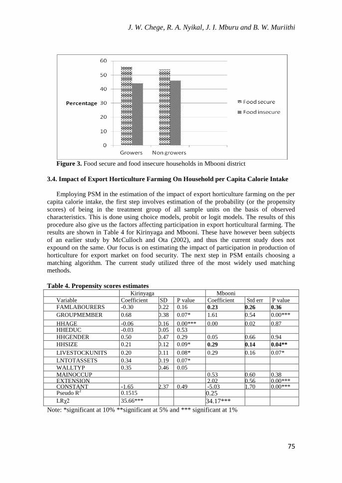
Based on the recommended per capita calorie intake of 2250 kcal, we can conclude from

the above analysis that both growers and non-growers of export horticulture in Kirinyaga are

food consuming enough. Furthermore, both groups were above the average dietary energy

requirement, thus can loosely be considered food secure. In contrast, both growers and non-

growers in Mbooni consumed less than the average dietary energy requirement, thus can be

considered as food insecure. Figure 2 and 3 illustrate the percentage food secure and food

insecure households in the two groups in Kirinyaga and Mbooni.

Figure 2. Food secure and food insecure households in Kirinyaga district


75

Figure 3. Food secure and food insecure households in Mbooni district

3.4. Impact of Export Horticulture Farming On Household per Capita Calorie Intake

Employing PSM in the estimation of the impact of export horticulture farming on the per

capita calorie intake, the first step involves estimation of the probability (or the propensity

scores) of being in the treatment group of all sample units on the basis of observed

characteristics. This is done using choice models, probit or logit models. The results of this

procedure also give us the factors affecting participation in export horticultural farming. The

results are shown in Table 4 for Kirinyaga and Mbooni. These have however been subjects

of an earlier study by McCulloch and Ota (2002), and thus the current study does not

expound on the same. Our focus is on estimating the impact of participation in production of

horticulture for export market on food security. The next step in PSM entails choosing a

matching algorithm. The current study utilized three of the most widely used matching

methods.

Table 4. Propensity scores estimates Kirinyaga Mbooni

Variable Coefficient SD P value Coefficient Std err P value

FAMLABOURERS -0.30 0.22 0.16

0.23 0.26 0.36

GROUPMEMBER 0.68 0.38 0.07* 1.61 0.54 0.00***

HHAGE -0.06 0.16 0.00*** 0.00 0.02 0.87 HHEDUC -0.03 0.05 0.53

HHGENDER 0.50

0.47 0.29 0.05 0.66 0.94

HHSIZE 0.21 0.12 0.09* 0.29 0.14 0.04**

LIVESTOCKUNITS 0.20 0.11 0.08* 0.29 0.16 0.07*

LNTOTASSETS 0.34 0.19 0.07*

WALLTYP 0.35 0.46 0.05

MAINOCCUP 0.53 0.60 0.38 EXTENSION 2.02 0.56 0.00*** CONSTANT -1.65 2.37 0.49 -5.03 1.70 0.00*** Pseudo R2

0.1515 0.25

LRχ2

35.66*** 34.17***

Note: *significant at 10% **significant at 5% and *** significant at 1%


76

Figure 4. Propensity score histogram Kirinyaga district

Figure 5. Propensity score histogram Mbooni district

.2 .4 .6 .8 1 Propensity Score

Untreated Treated

.2 .4 .6 .8 1 Propensity Score

Untreated Treated


77

The third step in PSM entails testing or checking overlap or the common support

condition. Implementing the common support condition ensures that any combination of

characteristics observed in the treatment group can also be observed among the control

group. The histograms in figure 4 and 5 show that the distribution of the propensity scores

between the groups of growers and non-growers in Kirinyaga and Mbooni respectively were

within the region of common support.

Once the common support condition is satisfied and matching algorithm chosen to match

the different scores of participants to those of non-participant, then treatment effect are

estimated. In Table 5 results show that the three matching methods used indicated positive

impact in Kirinyaga and a negative impact in Mbooni, with an average ATT of 264 Kcal and

-355 Kcal for Kirinyaga and Mbooni respectively. The result can be explained by the

differences in Agro-ecological zones of the two districts and the level of development of

irrigation networks. Mbooni is a semi-arid area with high incidence of poverty and often is

struck with famine from year to year. This is exacerbated by the poor if any irrigation and

infrastructural networks. Moreover, small holder horticultural farmers in Mbooni were

producing export horticulture on small land areas averaging 0.24 acres as opposed to 0.53 in

Kirinyaga. The results are thus in line with those of Kuhlgatz and Abdulai (2011) who

assessed the determinants and welfare impacts of export crop cultivation in Ghana, and

found that household welfare was hardly affected at low levels of export revenue shares, but

rose with increasing level of specialization. This suggests that there is a probable optimal

level of production that smallholder farmers ought to have to ensure benefits of export

horticulture participation are accrued. The marginal benefits from a low export intensity may

be easily outweighed by immeasurable benefits of non-export agriculture, such as

predictability of local markets and risk insurance through consumption of own produce.

Moreover, uncertainties about foreign markets especially the price levels, increased input

prices, reduced bargaining power, the private food safety standards that comes with a cost,

rejection of produce due to defects are all challenges faced by the export horticulture

farmers. These results coincide with those of Dewalt (1993), who after reviewing the results

of studies examining the impacts of agricultural commercialization on food consumption and

nutritional status concluded that increased income does not translate directly into increased

food consumption at either the household or individual level. The author concluded that

those schemes in which subsistence production were protected or stabilized are more likely

to show positive results with an increase in income generated from cash cropping.

Table 5. Treatment effects on Adult equivalent calorie intake (gamma level for

sensitivity analysis)

Kirinyaga Mbooni

Matching

Algorithm

ATT t

stat

Gamma level ATT t stat Gamma

level

NNM 263 2.00 1.9-1.95 -389 -2.29 2.65-2.7

KBM 267 2.02 1.65-1.7 -337 -2.06 2.3-2.35

RM 262 2.17 1.6-1.65 -341 -2.17 2.25-2.3

Mean 264 -355

Step 5 involves assessment of sensitivity analyses using Gamma levels. As presented in

Table 5 with the treatment effects Sensitivity analysis was conducted using Rosenbaum

bounds to ascertain the robustness of the estimates. The higher the gamma levels, the more

insensitive to hidden bias are the results. The goal is to determine how strongly an

unmeasured variable must influence the selection process to undermine the implications of

the matching process. The sensitivity analysis indicated that the estimated treatment effects


78

were insensitive to hidden bias with gamma values being from 1.9 to 1.95 for the nearest

neighbor matching, 1.65 to 1.7 for kernel based matching and 1.6 to 1.65 for the radius

matching in case of Kirinyaga. Estimated effects in Mbooni are even more insensitive to

hidden bias with gamma values being from 2.65 to 2.7 for the nearest neighbor matching, 2.3

to 2.35 for kernel based matching and 3.25 to 2.3 for the radius matching. These value imply

that, for instance in the case of Kirinyaga, nearest neighbor matching a gamma level of 1.9,

if individuals that have the same X vector differ in their odds of participation by a factor of

90 percent, the significance of the participation effect on per capita calorie intake may be

questionable. The implication is the same for the others. We can therefore conclude that

even considerable amount of unobserved heterogeneity would not alter the inference about

the estimated effects. In other words the average treatment effects are insensitive to hidden

bias.

The final step involves checking the matching quality. The basic idea of this step is to

compare the situation before and after matching and check if there remain any differences

after conditioning on the propensity score. One suitable indicator of balancing powers of the

estimations is ascertained by considering the reduction in the mean absolute standardized

bias between the matched and unmatched models as shown in Table 6. The high percentage

values of reduced standardized bias indicate the effectiveness of matching in reducing biases

in the estimates. Pseudo R2 from the propensity score estimation and from re-estimation of

the propensity score after matching are also presented together with the P values of the

likelihood ratio tests before and after matching. In all the different matching algorithms for

the two areas, the joint significance of the regressors hypothesis, is always rejected after

matching. However, the same hypothesis was never rejected at any significance level before

matching, suggesting that there is no systematic difference in the distribution of covariates

between adopters and non-adopters after matching in all the cases.

Table 6. Covariate Balancing Tests

Test indicator Kirinyaga Mbooni

Before matching

Mean bias before matching 29.19 32.38

Pseudo R2 0.1515 0.244

LR χ2 (P value) 35.22(0.000) 33.94(0.000)

After matching using nearest neighbor matching (NNM)

Mean bias after matching 6.55 10.80

Percentage bias reduced 78 67

Pseudo R2 0.05 0.05

LR χ2 (P value) 4.63(0.87) 7.95(0.44)

After matching using kernel based matching (KBM)



Pseudo R2 0.02 0.03

LR χ2 (P value) 6.22(0.72) 5.46 (0.70)

After matching using radius matching (RM)



Pseudo R2 0.03 0.04

LR χ2 (P value) 9.19 (0.42) 6.19(0.63)


79

4. Summary, Conclusion and Recommendations

Export horticulture farming can be considered a cash cropping system in Kenya. It is

ranked third in terms of foreign exchange earnings after tourism and tea. The contribution of

export horticulture to food intake and food security is less direct than that of domestic

horticultural products and staple crops that are readily consumed in the farm household.

Available evidence in the debate of the impact of cash cropping system on food security

shows mixed results. Both negative and positive impacts can be identified which vary with

choice of cash crops and the situation in which they are being grown and marketed. Review

of existing literature concludes that the available evidence is insufficient to draw strong

policy recommendations. The current study contributed to the existing literature by assessing

the impact of export horticultural farming, a major cash cropping practice in Kenya on the

food intake of smallholder farmers, in Mbooni district in Eastern Province a semi-arid area

and Kirinyaga district in Central district, which lies in the high potential zone as case studies.

Household per capita calorie intake was estimated using a seven-day recall method.

Smallholder farmers in Mbooni were found to be consuming less than enough food while

those of Kirinyaga were consuming enough. Participation in export horticulture farming had

a positive impact in Kirinyaga but negative impact in Mbooni. The results of the two

districts, which represent two diverse setting, can be generalized to represent their respective

provinces and any other part in Kenya or in East Africa with similar characteristics.

Mbooni smallholder farmers’ food consumption level for both growers and non-growers

of export vegetables should be addressed. Holding all factors constant, promotion of export

horticulture in the region may worsen the food insecurity situation. Alternative strategies to

ensure food security at household and district level should be promoted as well as

improvement of the road network, and irrigation in the area to ensure food and cash crops

production and marketing systems are well functioning.

A comprehensive evaluation on farming systems and gross margins of different scales of

export horticulture cultivation in Mbooni and probably other growing areas need to be

carried out. It may be more profitable to participate in domestic horticulture and staple food

production than engage in export horticulture farming in some areas considering the

infrastructure and the lack of reliable food marketing systems. Further research should also

consider assessing how income resulting from export horticulture farming is utilized as this

could also contribute to food insecurity in a household. Considering the positive impact of

participating in export horticulture production in Kirinyaga, on the per capita calorie intake,

smallholder farmers in this district and others with similar agro-ecological and socio

characteristics should be encouraged to participate in producing horticultural crops for the

export market.

Acknowledgements

This research was made possible by a grant from the International Development and

Research Centre (IDRC) through Dri-VLIC Kenya project and the African Economic

Research Consortium (AERC) through the Collaborative Masters in Agricultural and

Applied Economics (CMAAE) Programme. This support is greatly appreciated.

References

Anouk, P. (2010). Agro-export Specialization and Food Security in a Sub-national Context:

The Case of Colombian Cut Flowers: Cambridge Journal of Regions, Economy and

Society, 3(2), 279-294.

http://cjres.oxfordjournals.org/search?author1=Anouk+Patel-Campillo&sortspec=date&submit=Submit


80

Asfaw, S., Mithöfer, D. and Waibel, H. (2007). What Impact Are EU Supermarket Standards

Having on Developing Countries Export of High‐Value Horticultural Products? Evidence

from Kenya. Journal of International Food & Agribusiness Marketing, 22(3-4), 252-276.

Bolwig, S., & Odeke, M. (2007). Household food security effects of certified organic export

production in tropical Africa: A Gendered Analysis. Bennekom, Netherlands: Export

Promotion of Organic Production in Africa (Sida). from:

Caliendo, M., &Kopeinig, S. (2008). Some Practical Guidance for the Implementation of

Propensity Score Matching. Journal of Economic Surveys, 22, (1), 31–72.

Carletto, C., Zezza, A., & Banerjee, R. (2013). Towards better measurement of household

food security: Harmonizing indicators and the role of household surveys. Global Food

Security, 2(1), 30-40.

DeWalt, K. (1993). Nutrition and the Commercialization of Agriculture: Ten Years Later.

Social Science and Medicine Journal, 36(11), 1407-16.

Bongaarts, J. (2007). Food and Agriculture Organization of the United Nations: The State of

Food and Agriculture: Agricultural Trade and Poverty: Can Trade Work for the Poor?.

Population and Development Review, 33(1), 197-198.

Government of Kenya (GoK), (2012). National Horticulture Policy. Republic of Kenya.

Ministry of Agriculture, Nairobi.

Goverah, J., & Jayne, T. S. (1999). Effects of Cash Crop Production on Food Crop

Productivity In Zimbabwe: Synergies or Trade Offs. MSU International Development

Working Paper No. 74. East Lansing, Michigan: Michigan State University, Department

of Agricultural Economics.

Horticultural Crops Development Authority (HCDA) (2009). Horticultural Crops

Development Authority Strategic plan 2009-2013. Nairobi: Government Printer.

Heckman, J., Ichumura, H., & Todd, P. (1997). Matching as an Econometric Evaluation

Estimator: Evidence from Evaluating a Job Training Program. Review of Economic

Studies, 64(4), 605-654.

Hoddinott, J. (1999). Choosing Outcome Indicators of Household Food Security. Technical

Guide. No. 7. Washington, D.C: International Food Policy Research Institute.

Kennedy, E. T., & Cogill, B. (1987). Income and Nutritional Effects of the

Commercialization of Agriculture in South Western Kenya, 63. Washington, D.C:

International Food Policy Research Institute.

Kuhlgatz, C., & Abdulai, A. (2011). Determinants and Welfare Impacts of Export Crop

Cultivation – Empirical Evidence from Ghana. Paper presented in 2011 European

Association of Agricultural Economists Congress, August 30-September 2, 2011, Zurich,

Switzerland. .

Langat, B.K., Sulo, T. K., Nyangweso, P.M., Ngéno, V.K., Korir, M. K. & Kipsat, M. J.

(2010). Household Food Security in Commercialized Subsistence Economies: Factors

Influencing Dietary Diversity of Smallholder Tea Farmers in Nandi South, Kenya; Poster

presented in 2010 Joint 3rd African Association of Agricultural Economists (AAAE) and

48th Agricultural Economists Association of South Africa(AEASA) Conference, Cape

Town, South Africa.

Legge, A., Orchard, J., Graffham, A., Greenhalgh, P. & Kleih, U. (2006). The Production of

Fresh Produce in Africa for Export to the United Kingdom: Mapping Different Value

chains. Natural Resources Institute, UK.

McCulloch, N. & Ota, M. (2002). Export Horticulture and Poverty in Kenya. Institute for

Development Studies Working Paper,174,Brighton, UK.

Riely, F., Mock, N., Cogill B., Bailey, L., &Kenefick, E. (1999). Food Security Indicators

and Framework for Use in the Monitoring and Evaluation of Food Aid Programs. Food

and Nutrition Technical Assistance, Academy for Educational Development (AED)


81

Rosenbaum, P. R., & Rubin, D. B. (1983). The Central Role of the Propensity Score in

Observational Studies for Causal Effects. Biometrika, 70, (1), 41–55.

Santeramo, F. G. (2015). On the composite indicators for food security: decisions matter!

Food Reviews International, 31 (1), 63-73.

Schneider, K. & Gugerty, M. K. (2010). The Impact of Export Driven Cash Crops on

Smallholder Households. ESPAR Brief No. 94. Washington D. C., Evans School of

Policy Analysis and Research (ESPAR). Sen, A. (1981). Poverty and Famines: An Essay

on Entitlement and Deprivation. Oxford: University Press.

Sorre, B. (2011). Cash Crop Production, Food Security and Nutrition in Rural Households: A

Case of Sugarcane Production, Household Food Security and Nutritional Status in

Nambale Division, Busia District, Kenya. LAP LAMBERT Academic Publishing.

Swindale, A. & Bilinsky, P. (2006). Household Dietary Diversity Score (HDDS) for

Measurement of Household Food Access. Washington, D.C: Food and Nutrition

Technical Assistance Project ,Academy for Educational Development.

Von Braun, J. & Kennedy, E. (1986). Commercialisation of Subsistence Agriculture: Income

and Nutrition Effects in Developing Countries, Working Paper on Commercialisation of

Agriculture and Nutrition No. 1. Washington, D.C.: International Food Policy Research

Institute.

Webb, P., Coates, J., Frongillo E., Lorge Rogers, B., Swindale, A., & Bilinsky. P. (2006).

Measuring Household Food Insecurity: Why It’s so Important and yet so Difficult to Do.

Journal of Nutrition, 136(5),1404S-1408S.

impact of export horticulture farming on...

Documents