impact of hull propeller rudder interaction on ship...
TRANSCRIPT

178
Impact of Hull Propeller Rudder Interaction on Ship Powering Assessment
Charles Badoe, University of Southampton, United Kingdom,[email protected]
Stephen Turnock, University of Southampton, United Kingdom,[email protected]
Alexander Phillips, National Oceanography Centre, Southampton, United Kingdom, [email protected]
Abstract
It is the complex flow at the stern of a ship that controls the overall propulsive efficiency of the hull-
propeller-rudder system. This work investigates the different analysis methodologies that can be
applied for computing hull-propeller-rudder interaction. The sensitivity into which the interaction
between the propeller and rudder downstream of a skeg is resolved as well as varying the length of
the upstream skeg are also discussed including techniques to consider in such computations.
Throughout the work, the importance of hull-propeller-rudder interaction for propulsive power
enhancement is demonstrated. A final case study examines the performance of a twin skeg, twin screw
arrangement.
1. Introduction
Increasing the energy efficiency of a ship will play an ever greater part in the design process. The
design of the stern arrangement involving as it does the complex interaction between the hull wake,
propeller performance and use of a rudder for vessel control is the dominant factor in determining the
overall propulsive efficiency. The retrofit installation of energy saving devices or the improved
optimisation of the stern arrangement during concept and detailed design phases require much higher
fidelity analysis methods that have been conventionally applied.
The propulsive performance of a ship typically depends on how well the interaction between the hull,
propeller and rudder is understood, assessed and modelled (Molland & Turnock, 2007). Sakamoto et
al. (2013) state the relationship between the power delivered to the propeller in behind hull conditions
PD, the effective speed of a ship PE, and quasi propulsive efficiency 𝜂𝐷, may be expressed as:
𝑃𝐷 = 𝑃𝐸
𝜂𝐷 =
𝐶𝑤 + (1+𝑘)𝐶𝑓 + ∆𝐶𝑓
1−𝑡
1−𝑤𝑇 × 𝜂𝑅 × [
𝐽
2𝜋 ×
𝐾𝑇𝐾𝑄
]×
1
2𝜌𝑆𝑉𝑠
3 (1)
where 𝐶𝑤 is the ship wave-making resistance coefficient, k is the form factor of the ship, 𝐶𝑓 is the
frictional resistance coefficient, Δ𝑐𝑓 is the allowance correlation between model and ship, 𝑆 is the
wetted surface area of the ship, t is the thrust deduction fraction, which is the interaction between the
hull and propeller, 𝑤𝑇 is the wake fraction, which is the interaction between the hull and water, 𝜂𝑅 is
the relative rotative efficiency and takes account of the differences between the propeller in openwater
condition and when behind the hull, 𝜌 is the fluid density, J is the propeller advance coefficient, 𝐾𝑇 is
the propeller thrust coefficient, 𝐾𝑄 is the propeller torque coefficient.
1-t and 1- 𝑤𝑇 are interaction effects which play an important role in the overall powering of ships. For
example, examination of equation (1) indicates how 1-t can be maximized and 1- 𝑤𝑇 minimized to
reduce the delivered power 𝑃𝐷. As hull-propeller-rudder interaction is dependent on many features,
there is often scope for improvement in the overall ship powering process. The propeller performance
will depend on the inflow (hull wake) which is also dependent on the hull form. The rudder also has
to operate under the influence of the upstream hull and propeller.
This paper considers results on hull-propeller-rudder interaction and its impact on propulsive
performance. The discussion is made based on the research results of a three year project on the
‘Design Practice For The Stern Hull of Future Twin-Skeg Ships’at the University of Southampon,
UK. The first part of the paper reviews approaches to hull-propeller rudder analyses, including
various methodologies that have been used for such successful analyses, associated cost in

179
computation and the suitability for design purposes. The paper does not go into details of all
approaches, but provides references for a more profound discussion.
The second part of the paper reviews a case study into the sensitivity into which the interaction
between the propeller and rudder downstream of a skeg is resolved as well as varying the length of the
upstream skeg. The computed results are compared to a detailed wind tunnel investigation, which
measured changes in propeller thrust, torque and rudder forces. Variation of the upstream skeg length
effectively varies the magnitude of the crossflow and wake at the propeller plane. A mesh sensitivity
study quantifies the necessary number of mesh cells to adequately resolve the entire flow field. In
addition, analysis is conducted on parameters such as propeller and rudder forces and rudder pressure
distributions from the computation of the interaction between the skeg, rudder and propeller. The
computational expense associated with the time resolved propeller interaction was identified as one of
the major problems of the hydrodynamic analysis.
Lastly, based on the experience drawn from the above mentioned analysis, techniques to consider for
hull-propeller-rudder applications such as a twin skeg, twin screw vessel are discussed, this includes
the influence of small details that are easily not included in such computations, but can result in
changes in flow characteristics as well as changes in propulsive power.
2. Approaches and methodologies
Flow analysis of a ship stern to gain an understanding of the interaction between the hull, propeller
and rudder for performance improvement is a challenging task from a numerical point of view. The
most interesting and challenging aspect of such analysis is the influence of the propeller action and
the unsteady hydrodynamics of the rudder working in the propeller wake. One approach to address the
problem is to adopt a direct method where the propeller and farfield domains are joined using a rotor-
stator method (L��bke, 2005). The propeller is rotated at each time step and the interface between the
two domains is achieved using a sliding mesh interface. To ensure the flow structure generated around
the propeller are correctly transferred to the stationary domain, a fine mesh is required at the interface.
This approach theoretically offers the highest degree of fidelity, but requires small time steps due to
restrictions imposed by explicitly solving the propeller flow, thus placing a high demand on
computation.
The next level of complexity involves using an indirect approach by coupling a lower fidelity
propeller code (potential flow code, blade element momentum BEMt code etc.) with a CFD solver.
The propeller code utilises the non-uniform inflow at the propeller plane calculated from the RANS
simulation to determine the thrust and torque as well as its distribution. This is then represented in the
RANS simulation by momentum source terms. Such an approach alleviates some of the time step and
mesh restrictions. This has been used by Simonsen and Stern (2003) to simulate the manoeuvring
characteristic of the Esso Osaka with a rudder. In their formulation the propeller was represented by
bound vortex sheets placed at the propeller plane and free vortices shed downstream of it. BEMt was
used by Phillips et al. (2009) amongst others to evaluate the momentum terms.
The lowest level of complexity involves the use of a prescribed body force approach where the impact
of the propeller on the fluid is represented as a series of axial and tangential momentum sources. This
is the simplest of the discussed methods, although more simplified first order methods also exist. For
instance the approach with a uniform thrust distribution that has been used by Philips et al. (2010) and
which assumes a force only in the axial direction.
Badoe et al. (2014) investigated the three-way interaction between the hull, propeller and rudder by
replicating experiments performed by FORCE Technology for a container ship operating at a Froude
number of 0.202. The ability of three different methods were compared, namely; prescribed body
force approach (RANS-HO), Two-way coupled RANS-BEMt model (RANS-BEMt) and a discretised
propeller approach or direct method (AMI). This was validated against experimental data from the
SIMMAN 2014 workshop on verification and validation of ship manoeuvring simulation methods,

180
SIMMAN (2014). Differences between the various methods were outlined quantitatively. The results
demonstrated that as long as the radial variation in both axial and tangential momentum generated by
the propeller are included in the computations, then the influence of the unsteady propeller flow can
be ignored and a steady computation performed to evaluate the propeller influence on the hull and
rudder. Below are other conclusions drawn from the study regarding the various methods:
(a) Fluid dynamic fidelity
RANS-HO assumes a constant circumferential distribution of thrust and torque, hence do not
capture all aspects of hull-propeller-rudder interaction effects, especially the interaction
between the hull on propeller and rudder on propeller and vice versa. The method was also
poor in replicating the swirl effect which resulted in a different flow field (i.e. symmetry in
the flow field).
RANS-BEMt is best suited for capturing and predicting most aspects of hull-propeller-rudder
interaction effects. The method calculates the thrust and torque as part of the simulation and is
able to replicate the swirl effect much better than RANS-HO.
AMI theoretically offers the highest degree of fidelity, however, it requires small time steps
due to restrictions imposed by explicitly solving the propeller flow.
(b) Computational cost
RANS-HO is the least costly, can be used for quick resistance and self-propulsion estimations
only if the flow field details are not of prime importance.
RANS-BEMt follows on from RANS-HO as being less costly for ship resistance and
propulsion simulations with less than 0.27% of the total simulation (of 6 wall clock hours)
spent on propeller modelling.
AMI is the most computationally demanding approach (typically ≥ 30% of the total
simulation time for similar setup with RANS-BEMt) since the full transient flow field needs
to be resolved with a higher level of mesh cells in order to provide accurate estimates of
resistance and propulsion parameters. The method does not only suffer from long overall
simulation time, but also from increased computational time per time step.
(c) Suitability for design purposes
RANS-HO reasonably predicted the global forces compared to the experiment, but was poor
in replicating the flow field as such the method may be used for initial assessment of ships
resistance and propulsion where requirement for exact mirroring of the flow fields are not
essential.
RANS-BEMt was able to predict the resistance and propulsion parameters much better, but
the propeller influence has been averaged over one blade passage which neglects tip and hub
vortices, this makes it unsuitable for cavitation analysis. The methods may, however benefit
from the addition of tangential inflow conditions and coupled with the non–uniform inflow
inputs may be suitable for transient manoeuvring simulations as well as resistance and
powering computations.
AMI is more suitable for all the analysis described above, but requires experience in the use
and distribution of high mesh cells to capture detail flow features.

181
3 Case studies
3.1. Skeg-rudder-propeller interaction review
As an example, a skeg-propeller-rudder interaction investigations in straight ahead condition and drift
angle is presented (see Badoe et al. 2015a for full details of the study). An open source flow solver
was used to investigate the sensitivity into which the interaction between the propeller and rudder
downstream of a skeg is resolved as well as varying the length of the upstream skeg. In simulating the
skeg, rudder and propeller flow, the entire flow field was considered as a result of the oblique motion
and rotation induced by the propeller. A discretised propeller approach which uses the arbitrary mesh
interface technique (AMI) was used to account for the action of the rotating propeller. Due to the
complexity of the propeller geometry, especially around the blade tip with very small thickness, it was
possible to place only two prism layers on the propeller. The surface refinement for the propeller was
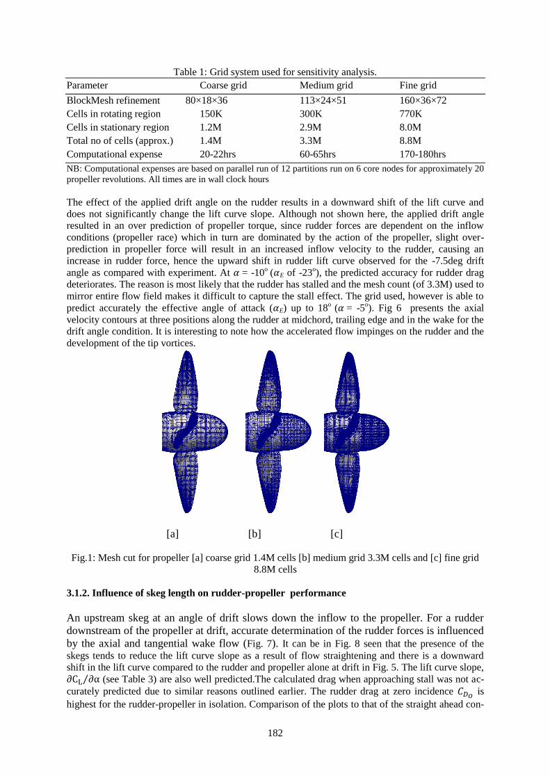
however increased to ensure that most of the flow features were resolved. Fig. 1 shows the different
meshes generated on the propeller. Tables 1&2 show the details of the grid system along with
predicted thrust and torque computed on each grid as well as viscous and pressure contributions to the
total drag. Rudder lift and drag values are also presented for Simonsen (2000) and Philips et al.
(2010) who both performed similar investigations for straight ahead conditions (no applied angle of
drift) using the CFDSHIP-IOWA and ANSYS CFX code respectively, and using a body force
propeller model with load distribution based on the Hough and Ordway(HO) (1965) thrust and torque
distribution.
The difficulty associated with rudder drag prediction is evident in the results. This is mainly due to the
difficulty associated with replicating the influence of swirl on the local incidence angle. At high thrust
loadings, swirl components increases, leading to a reduction in the drag experienced by the rudder, the
mechanism is illustrated in Fig. 2. Simonsen (2000) outlined other reasons for drag coefficient over
prediction. Since the x-component of the normal to the rudder surface is large at the leading edge, the
pressure contribution is dominant for the local drag coefficient in this region, therefore if the leading
edge pressure and suction peaks are not adequately resolved it could lead to discrepancies in drag
coefficient. Although the detail local flow features such as the tip and hub vortices (which are useful
for cavitation analysis) described above will not be captured by the level of grid used, for
manoeuvring performance of the rudder exact “mirroring” of the flow field is not essential as long as
the required condition of flow (head) are adequately captured. Phillips et al. (2009) highlights the
difficulties in the prediction of propeller torque and rudder forces with large uncertainties and
comparison errors between calculated and experimental result unless significantly larger meshes are
used. Wang and Walters (2012) indicated values in excess of 22M to resolve propeller forces, whilst
Date and Turnock (2002) indicates values of 5-20M cells to fully resolve the rudder forces. However,
a good level of understanding of the global forces required for rudder and propeller forces during
manoeuvring may be obtained with the level of mesh resolution. Wall effects also play a defining role
in rudder drag prediction as has been addressed by H��erner (1965) who showed that due to root
vortex the drag of wall mounted experimental rudder differs from that of numerical rudder. Because
the propeller was working close to the wind tunnel floor, it could have influenced the root flow, hence
the root vortex and rudder drag prediction. Figs. 3&4 show the rudder forces for rudder angle 𝛼 = -
10.4o, -0.4
o, and 9.6
o. The results show improvement in the fine grid, especially for the drag
coefficient.
3.1.1. Influence of propeller on rudder in straight ahead condition and at drift
The global forces for the rudder and propeller combination in isolation at straight ahead and drift
angle conditions is shown in Fig. 5. Results for the straight ahead condition demonstrates that the
wake field generated by the propeller compares well with experimental values of lift and drag on a
rudder placed aft of the propeller at different angles of incidence.The influence of drift angle is well
captured in terms of rudder lift and drag characteristics.
182
Table 1: Grid system used for sensitivity analysis.
Parameter Coarse grid Medium grid Fine grid
BlockMesh refinement 80×18×36 113×24×51 160×36×72
Cells in rotating region 150K 300K 770K
Cells in stationary region 1.2M 2.9M 8.0M
Total no of cells (approx.) 1.4M 3.3M 8.8M
Computational expense 20-22hrs 60-65hrs 170-180hrs
NB: Computational expenses are based on parallel run of 12 partitions run on 6 core nodes for approximately 20
propeller revolutions. All times are in wall clock hours
The effect of the applied drift angle on the rudder results in a downward shift of the lift curve and
does not significantly change the lift curve slope. Although not shown here, the applied drift angle
resulted in an over prediction of propeller torque, since rudder forces are dependent on the inflow
conditions (propeller race) which in turn are dominated by the action of the propeller, slight over-
prediction in propeller force will result in an increased inflow velocity to the rudder, causing an
increase in rudder force, hence the upward shift in rudder lift curve observed for the -7.5deg drift
angle as compared with experiment. At 𝛼 = -10o
(𝛼E of -23o), the predicted accuracy for rudder drag
deteriorates. The reason is most likely that the rudder has stalled and the mesh count (of 3.3M) used to
mirror entire flow field makes it difficult to capture the stall effect. The grid used, however is able to
predict accurately the effective angle of attack (𝛼E) up to 18o
(𝛼 = -5o). Fig 6 presents the axial
velocity contours at three positions along the rudder at midchord, trailing edge and in the wake for the
drift angle condition. It is interesting to note how the accelerated flow impinges on the rudder and the
development of the tip vortices.
[a] [b] [c]
Fig.1: Mesh cut for propeller [a] coarse grid 1.4M cells [b] medium grid 3.3M cells and [c] fine grid
8.8M cells
3.1.2. Influence of skeg length on rudder-propeller performance
An upstream skeg at an angle of drift slows down the inflow to the propeller. For a rudder
downstream of the propeller at drift, accurate determination of the rudder forces is influenced
by the axial and tangential wake flow (Fig. 7). It can be in Fig. 8 seen that the presence of the
skegs tends to reduce the lift curve slope as a result of flow straightening and there is a downward
shift in the lift curve compared to the rudder and propeller alone at drift in Fig. 5. The lift curve slope,
∂CL ∂α⁄ (see Table 3) are also well predicted.The calculated drag when approaching stall was not ac-
curately predicted due to similar reasons outlined earlier. The rudder drag at zero incidence 𝐶𝐷𝑂 is
highest for the rudder-propeller in isolation. Comparison of the plots to that of the straight ahead con-

183
dition in Fig 4 shows that the asymmetry in the flow results in a shift in the performance of the rudder
which increases with increasing upstream skeg length.This shift may depend on the angle of drift.
Table 2: Detailed grid analysis for propeller and rudder forces, 𝛼= 10o, βR = 0
o, J = 0.36.
Grid Coarse Medium Fine Simonsen Phllips Data
grid grid grid (2000) (2010)
KT 0.305 0.294 0.286 0.283
ε +7.77% +3.89% +1.06%
KQ 0.051 0.047 0.044 0.043
ε +18.60% +9.30% +2.32%
CL 1.350 1.280 1.220 1.270 1.360 1.251
ε +7.96% +2.36% -2.44% +1.56% +8.76%
CD total 0.190 0.170 0.148 0.070 0.187 0.109
ε +74.3% +55.96% +35.78% -93.58% 71.56
CD viscous 0.075 0.072 0.069
CD pressure 0.115 0.098 0.079
At x = 1.05 chords, the propeller swirl dominates the flow, the rudder wake has mixed with the
surrounding faster moving fluid. The overall results provide reasonable initial estimates for rudder
forces at drift angle 𝛽𝑅 = −7.50 and 0o. Overall improvements in mesh resolution around the
propeller, rudder and rudder tip vortices would improve the quality of the results.
Fig.2: [a] Rudder angle zero degrees: forces due to propeller-induced incidence [b] Rudder angle zero:
forces due to propeller-induced incidence - high thrust loading, source: Molland and Turnock (2007).
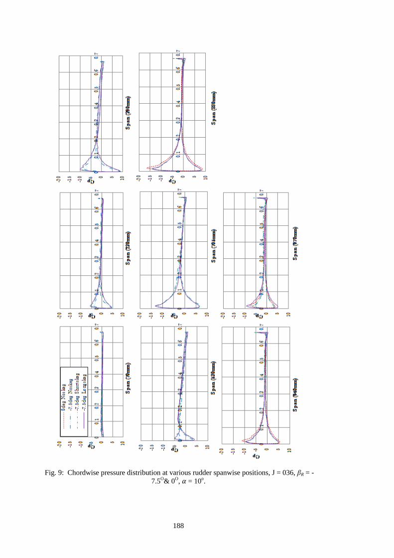
3.1.3. Rudder pressure distribution at straight ahead and at drift conditions
The influence of the propeller and skeg on rudder at straight ahead and drift conditions are compared
through chordwise pressure distribution of surface pressures for eight spanwise rudder locations from
the root to tip in Fig. 9. The computed chordwise pressure distribution represented by the local
pressure coefficient Cp is given by:
Cp =𝑃−𝑃∞
0.5𝜌𝑈2 (2)
where 𝑃 − 𝑃∞ is the local pressure; ρ is the density of air and U is the free stream velocity. Drift angle
influence can be observed for most areas of the rudder span below the center of the slipstream (below
the hub). Close to the slipstream, (span 230 & 390mm) local incidence resulted in the pressure peak
increasing with increasing skeg lengths at the rudder leading edge. An area of interest was just around

184
the hub where the unsteadiness in the flow introduced by the hub vortex can be observed for span
530mm as a bulge in the pressure curve for the zero drift angle around the rudder trailing edge. This
was not observed for the drift cases. In areas close to the tip (span 705mm-970mm) there were little
or no differences in pressure curves for the drift cases. This is also seen in the streamlines passing
through the short skeg at drift, Fig. 7 where most of the flow changes occur in the rudder mid span,
explaining why there was little difference in pressure curves for the drift cases around the rudder tip.
Table 3: Rudder lift curve slope, 𝜕CL/𝜕𝛼, and corresponding drag at zero incidence,CDO.
CDO 𝜕CL/𝜕𝛼
Molland&Turnock Calculations Molland&Turnock Calculations
Zero drift angle 0.016 0.02 0.132 0.129
Rudder&propeller alone 0.083 0.06 0.146 0.144
Short length skeg 0.029 0.01 0.121 0.119
Medium length skeg 0.025 0.012 0.119 0.115
Long length skeg 0.0169 0.019 0.125 0.126
Fig.3: Rudder drag coefficient, βR = 0O, J = 0.36.
Fig.4: Rudder lift coefficient, βR = 0O, J = 0.36.
-0.2
0
0.2
0.4
0.6
-24 -18 -12 -6 0 6 12 18 24
CD
Rudder angle,α (deg)
Molland&Turnock(1991) Coarse grid
Medium grid Fine grid
Phillips(2009) Simonsen(2000)
-4
-2
0
2
4
-24 -18 -12 -6 0 6 12 18 24
CL
Rudder angle,α (deg)
Molland&Turnock(1991) Coarse gridMedium grid Fine gridPhillips(2009) Simonsen(2000)

185
Fig.5: Effect of drift angle on the performance of a rudder and propeller combination in isolation at
J = 0.36, βR = -7.5O (medium grid results) and βR = 0
O (fine grid results).
[a] x = 0.60chords (rudder mid chord) [b] x = 0.90chords (rudder trailing edge) [c] x = 1.05 chords (rudder wake)
Fig.6: Axial velocity contours at different rudder x-positions, J = 0.36, 𝛽𝑅 =-7.5
o at 𝛼 = 10
o.
0
0.4
0.8
1.2
1.6
2
-40 -30 -20 -10 0 10 20 30 40
CD
Rudder angle,α (deg)
-7.5 deg drift angle Molland&Turnock(1995)
-7.5deg drift angle AMI
0 deg drift angle Molland&Turnock(1995)
0 deg drift angle AMI
-6
-4
-2
0
2
4
6
8
-40 -30 -20 -10 0 10 20 30 40
CL
Rudder angle,α (deg)
-7.5deg drift angle Molland&Turnock(1995)
-7.5deg drift angle AMI
0 deg drift angle Molland&Turnock(1995)
0 deg drift angle AMI

186
Fig.7: Streamlines passing through the shortskeg, J = 0.36, βR = -7.5O at 𝛼 = 10
o.
3.2. Techniques to consider for effective hull-propeller-rudder computations
Various techniques to consider in ship powering based computations, including small details
that can result in changes in flow characteristics as well as changes in propulsive power:
High fidelity computations
Using Reynolds Averaged Navier Stokes solvers (RANS) to analyse hull-propeller-rudder
require high fidelity computations as the boundary layer of the hull, skeg and the viscous
wake needs to be captured with high level of accuracy. Here, high fidelity refers to RANS
solvers which employ good grids and strong turbulence models. The skeg and hull flow may
be characterised by complex vortex shedding, which may require complex grid resolution in
order to understand them. Eça et al. (2002) showed that numerical simulation of such flows
require grids with orthogonality at the ship surface where the no-slip condition is applied and
high stretching of the grid towards that surface to resolve the flow in the near-wall region.
The mesh in the propeller plane should be able to give circumferential distribution of the three
components of the velocity as this information forms an important part of the input to the
propeller. It is not always the size of the grid that determines the accuracy of the solution but
its distribution so as to provide useful information of the underlying physics of the flow.
What if the self-propelled thrust is over estimated ?
Reference is hereby made to Badoe et al. 2015b who focussed on calm water powering
performance of a future twin skeg LNG ship specifically on the changes in propulsive power
resulting from small variations in design. The influence of free surface was not included in
the computations. A ‘RANS-BEMt’ approach was utilized for the self-propelled
computations. The self-propulsion point was realised by manually adjusting the propeller
revolutions until the self-propelled thrust (Tsp) equals the self-propelled drag (Rsp) or Tsp -
Rsp = 0, similar to actual model test procedures. Fig. 10 shows the impact on thrust deduction
when the self-propelled thrust is over-estimated. From the plot, it can be seen that a linear
relation exists between self-propelled thrust prediction and its impact on thrust deduction. For
example, from the results, an error of the self-propelled thrust by say 7% will result in an
error in the thrust deduction by approximately 7%. It should however be pointed out that this
relation has been found based on constraints placed on the hull and the use of nominal wake
values as input to the propeller code.
Tangential wake effects
A disadvantage with the equipment of skegs is that they have a high wetted surface area,
hence increasing frictional resistance. But as may be seen from the streamline plot in Fig. 11,
the presence of the skegs provides pre swirl to the propeller. This is advantageous for the

187
propeller performance as it can contribute to improving the propeller efficiency,compensating
for increase in frictional resistance. Most self-propelled twin skeg computations using a body
force propeller model only consider the effect of axial wake as that is the predominant
component as far as most propeller straight ahead flows are concerned. Usually, an upward
flow exists at the aft end which leads to an axial flow component plus a tangential flow
component (Molland et al. 2011). The influence of tangential wake was studied by Badoe et
al. 2015b for a twin skeg ship as shown in Fig. 12. The plots were taken at 0.18D behind the
propeller plane (see Fig.13). The influence of tangential wake investigated showed that by
considering the upward flow the true axial component is slightly over-predicted, both the
radial and tangential components of wake are modified thus modifying the thrust deduction
and hence the propulsive efficiency.
Fig. 8: Effect of drift angle rudder downstream of 3 skeg configurations at J = 0.36, 𝛽𝑅 = −7.50
0
0.2
0.4
0.6
0.8
1
1.2
-30 -20 -10 0 10 20 30
CD
Rudder angle,α (deg)
Shortskeg Molland&Turnock(1995)Shortskeg AMIMediumskeg Molland&Turnock(1995)Mediumskeg AMILongskeg Molland&Turnock(1995)Longskeg AMINoskeg Molland&Turnock(1995)Noskeg AMI
-4
-2
0
2
4
-30 -20 -10 0 10 20 30
CL
Rudder angle, (deg)
Shortskeg Molland&Turnock(1995)Shortskeg AMIMediumskeg Molland&Turnock(1995)Mediumskeg AMILongskeg Molland&Turnock(1995)Longskeg AMINoskeg Molland&Turnock(1995)Noskeg AMI
188
Fig. 9: Chordwise pressure distribution at various rudder spanwise positions, J = 036, βR = -
7.5O& 0
O, 𝛼 = 10
o.

189
Fig. 10: Error margin in thrust deduction prediction
[a]
[b]
Fig. 11: Streamlines passing through twin skegs at loaded draught, Fn = 0.197 [a] view from stern [b]
view from bottom.
0.08
0.12
0.16
0.2
0 5 10 15 20 25 30
t
(Tsp-Rsp/Tsp) x100

190
Fig. 12: Wake cut at 0.18D behind propeller plane [top] fixed z and varied y [bottom] fixed y and
varied z, for loaded draught condition, port side propeller. NB: solid lines represent the addition of
tangential wake effect and dotted lines represent no addition of tangential wake effect.
Fig. 13: Wake cut location for plots of velocity at 0.18D behind propeller plane
4 Conclusions
In the present paper, the impact of hull-propeller-rudder interaction on ship powering has been
presented. Various methodologies which have been used for such successful analysis were discussed
along with results into the sensitivity into which the interaction between the propeller and rudder
downstream of a skeg is resolved as well as varying the length of the upstream skeg. Overall, good
agreement was found between the experimental and computational results when predicting the
influence of the skeg and propeller on rudder. However, it can be seen that there is a significant
computational expense associated with a time resolved propeller interaction and that alternate body
force based methods are likely to still be required for hull(and skeg) -propeller-rudder computations.
-1
-0.5
0
0.5
1
-1 -0.5 0 0.5 1 1.5 2r/R
-1
-0.5
0
0.5
1
-1 -0.5 0 0.5 1 1.5 2
r/R
u/U, v/U, w/U
u/U
v/U
w/U

191
References
BADOE, C.; WINDEN, B.; LIDTKE, A.K.; PHILLIPS, A.B.; HUDSON, D.A.; TURNOCK, S.R.
(2014), Comparison of various approaches to numerical simulation of ship resistance and propulsion,
SIMMAN 2014, Lyngby
BADOE, C.; PHILLIPS, A.B.; TURNOCK, S.R. (2015), Influence of drift angle on the computation
of hull–propeller-rudder interaction, J.Ocean Eng. 103, pp.64-77
BADOE, C. (2015), Design practice for the stern hull of a future twin-skeg ship using a high fidelity
numerical approach, PhD Thesis, University of Southampton
DATE, J.C.; TURNOCK, S.R. (2002), Computational evaluation of the periodic performance of a
NACA 0012 fitted with a Gurney flap. J. Fluids Eng. 124, pp.227-234
EÇA, L.; HOEKSTRA, M.; WINDT, J. (2002), Practical Grid Generation Tools with Applications to
Ship Hydrodynamics, 8th Int. Conf. in Grid Generation in Computational Field Simulations, Hawaii
HOERNER, S. F. (1965), Fluid dynamic drag, Midland Park, New Jersey
HOUGH, G.R.; ORDWAY, D.E. (1965), The generalized actuator disc. Dev. in Theor. and Appl.
Mech. 2, pp.317-336
LUBKE, L. (2005), Numerical simulation of flow around the propelled KCS, CFD Workshop Tokyo,
Tokyo, pp.587-592
MOLLAND, A.F.; TURNOCK, S.R.. (2007), Marine rudders and control surfaces: principles, data,
design and applications, Butterworth-Heinemann, Oxford
MOLLAND, A.F.; TURNOCK, S.R.; HUDSON, D.A. (2011), Ship resistance and propulsion:
practical estimation of ship propulsive power, University Press, Cambridge
PHILLIPS, A.B.; TURNOCK, S.R.; FURLONG, M.E. (2009), Evaluation of manoeuvring
coefficients of a self-propelled ship using a blade element momentum propeller model coupled to a
Reynolds averaged Navier Stokes flow solver, J. Ocean Eng. 36/15, pp.1217-1225
PHILLIPS, A.B.; TURNOCK, S.R.; FURLONG, M.E. (2010), Accurate capture of rudder-propeller
interaction using a coupled blade element momentum-RANS approach, Ship Technology Research
57/2, pp.128-139
SAKAMOTO, N.; KAWANAMI, Y.; UTO, S.; SASAKI, N. (2013), Estimation of Resistance and
Self-propulsion characteristics for a Low L/B Twin-Skeg Container Ship by High- Fidelity RANS
Solver, J. Ship Research, 57/1, pp.24-41
SIMMAN (2014), Workshop on verification and validation of ship manoeuvring simulation methods,
Lyngby
SIMONSEN, C. ( 2000), Propeller–Rudder Interaction by RANS, Ph.D thesis, University of Denmark
SIMONSEN, C.; STERN, F. (2003), Verification and Validation of RANS manoeuvring simulation of
Esso Osaka: effects of drift and rudder angle on forces and moments. J. Computers and Fluids 32,
pp.1325-1356
WANG, X.; WALTERS, K. (2012), Computational analysis of marine propeller performance using
transition-sensitive turbulence modelling, J.Fluids Eng. 134/7, pp.071107