impact of load-based nic-bonding scheduling on out...

IMPACT OF LOAD-BASED NIC-BONDING

SCHEDULING ON OUT-OF-ORDER DELIVERED

TCP PACKETS

by

Sumedha Gupta

B.S. in Electronics and Telecommunication, IITT College of

Engineering, 2003

Submitted to the Graduate Faculty of

the School of Information Sciences in partial fulfillment

of the requirements for the degree of

M.S. in Networking and Telecommunication

University of Pittsburgh

2010

UNIVERSITY OF PITTSBURGH

SCHOOL OF INFORMATION SCIENCES

This thesis was presented

by

Sumedha Gupta

It was defended on

Apr 16, 2010

and approved by

Richard Thompson, Ph. D., Professor

KyoungSoo Park, Ph. D., Professor

Abdelmounaam Rezgui, Ph. D., Professor

Co-Advisor: KyoungSoo Park, Ph. D., Professor

Thesis Advisor: Richard Thompson, Ph. D., Professor

ii

IMPACT OF LOAD-BASED NIC-BONDING SCHEDULING ON

OUT-OF-ORDER DELIVERED TCP PACKETS

Sumedha Gupta, M.S.

University of Pittsburgh, 2010

The highest NIC bonding performance is achieved by the round-robin scheduling mode.

However, we found that the performance was much lower than the theoretical limit due

to out-of-order TCP packet delivery. So our work proposes a load-balanced NIC bonding

scheduling approach as a significant improvement over the current state-of-the-art. We pro-

pose that the outgoing packets should be queued on interfaces with the least amount of

packets waiting to be sent. This allows the load to be well balanced over all interfaces

thereby reducing the probability of packets arriving out-of-order at their destination. This

work presents an analysis of all currently available NIC bonding modes in terms of perfor-

mance. A new bonding simulation framework was developed to facilitate the development of

alternate scheduling algorithms and compare their performance. This helped us analyze and

propose load-based scheduling as a better alternative to the most popularly used round-robin

scheduling mode.

Keywords: NIC Bonding, Bonding Simulation, Trunking, LAG.

iii

TABLE OF CONTENTS

PREFACE . . . . . . . . . . . . . . . . . . . . . . . . . . . . . . . . . . . . . . . . . ix

1.0 INTRODUCTION . . . . . . . . . . . . . . . . . . . . . . . . . . . . . . . . . 1

1.1 NIC Bonding . . . . . . . . . . . . . . . . . . . . . . . . . . . . . . . . . . . 2

1.1.1 History . . . . . . . . . . . . . . . . . . . . . . . . . . . . . . . . . . . 3

1.1.2 Current Practice . . . . . . . . . . . . . . . . . . . . . . . . . . . . . . 3

1.2 Motivation . . . . . . . . . . . . . . . . . . . . . . . . . . . . . . . . . . . . 4

1.3 Thesis Organization . . . . . . . . . . . . . . . . . . . . . . . . . . . . . . . 5

2.0 BACKGROUND . . . . . . . . . . . . . . . . . . . . . . . . . . . . . . . . . . 6

2.1 NIC Bonding Modes . . . . . . . . . . . . . . . . . . . . . . . . . . . . . . . 6

2.1.1 Balanced-Round Robin . . . . . . . . . . . . . . . . . . . . . . . . . . 7

2.1.2 Active Backup . . . . . . . . . . . . . . . . . . . . . . . . . . . . . . . 7

2.1.3 Balanced-XOR . . . . . . . . . . . . . . . . . . . . . . . . . . . . . . . 8

2.1.4 Broadcast . . . . . . . . . . . . . . . . . . . . . . . . . . . . . . . . . 8

2.1.5 802.3ad . . . . . . . . . . . . . . . . . . . . . . . . . . . . . . . . . . . 9

2.1.6 Balance - TLB . . . . . . . . . . . . . . . . . . . . . . . . . . . . . . . 9

2.1.7 Balance - ALB . . . . . . . . . . . . . . . . . . . . . . . . . . . . . . . 10

2.2 Tradeoffs . . . . . . . . . . . . . . . . . . . . . . . . . . . . . . . . . . . . . 10

3.0 BONDING IN LINUX KERNEL . . . . . . . . . . . . . . . . . . . . . . . 13

3.1 Bonding driver . . . . . . . . . . . . . . . . . . . . . . . . . . . . . . . . . . 13

3.2 Bonding Configuration on Linux . . . . . . . . . . . . . . . . . . . . . . . . 16

4.0 THROUGHPUT MEASUREMENT . . . . . . . . . . . . . . . . . . . . . . 19

4.1 Experimental Setup . . . . . . . . . . . . . . . . . . . . . . . . . . . . . . . 19

iv

4.2 Switch Configuration . . . . . . . . . . . . . . . . . . . . . . . . . . . . . . . 19

4.3 Measurements . . . . . . . . . . . . . . . . . . . . . . . . . . . . . . . . . . 20

4.4 Throughput with Flexiclient suite . . . . . . . . . . . . . . . . . . . . . . . . 21

4.4.1 Throughput without bonding . . . . . . . . . . . . . . . . . . . . . . . 22

4.4.2 Round Robin throughput with bonding . . . . . . . . . . . . . . . . . 23

4.4.3 Active Backup throughput with bonding . . . . . . . . . . . . . . . . 23

4.4.4 XOR throughput with bonding . . . . . . . . . . . . . . . . . . . . . . 23

4.4.5 Broadcast throughput with bonding . . . . . . . . . . . . . . . . . . . 24

4.4.6 802.3ad throughput with bonding . . . . . . . . . . . . . . . . . . . . 24

4.4.7 TLB throughput with bonding . . . . . . . . . . . . . . . . . . . . . . 25

4.4.8 ALB throughput with bonding . . . . . . . . . . . . . . . . . . . . . . 25

4.4.9 Bonding throughput summary . . . . . . . . . . . . . . . . . . . . . . 25

5.0 BONDING SIMULATOR . . . . . . . . . . . . . . . . . . . . . . . . . . . . 27

5.1 Key features . . . . . . . . . . . . . . . . . . . . . . . . . . . . . . . . . . . 27

5.2 Design . . . . . . . . . . . . . . . . . . . . . . . . . . . . . . . . . . . . . . . 28

5.3 Implementation . . . . . . . . . . . . . . . . . . . . . . . . . . . . . . . . . . 30

5.3.1 Bonding simulator . . . . . . . . . . . . . . . . . . . . . . . . . . . . . 31

5.3.2 Request generator . . . . . . . . . . . . . . . . . . . . . . . . . . . . . 32

5.3.3 Scheduler . . . . . . . . . . . . . . . . . . . . . . . . . . . . . . . . . . 33

5.3.3.1 Round-robin scheduling . . . . . . . . . . . . . . . . . . . . . 35

5.3.3.2 Load-based scheduling . . . . . . . . . . . . . . . . . . . . . . 36

5.3.4 Interfaces . . . . . . . . . . . . . . . . . . . . . . . . . . . . . . . . . . 37

5.3.5 Clients . . . . . . . . . . . . . . . . . . . . . . . . . . . . . . . . . . . 38

5.3.6 Post-processing . . . . . . . . . . . . . . . . . . . . . . . . . . . . . . 39

5.3.6.1 Statistics . . . . . . . . . . . . . . . . . . . . . . . . . . . . . . 40

5.3.6.2 Visual graphs . . . . . . . . . . . . . . . . . . . . . . . . . . . 40

6.0 ANALYSIS AND RESULTS . . . . . . . . . . . . . . . . . . . . . . . . . . . 41

6.1 Analysis of scheduling algorithms . . . . . . . . . . . . . . . . . . . . . . . . 41

6.1.1 Round Robin . . . . . . . . . . . . . . . . . . . . . . . . . . . . . . . . 42

6.1.2 Load Based . . . . . . . . . . . . . . . . . . . . . . . . . . . . . . . . . 43

v

6.2 Results . . . . . . . . . . . . . . . . . . . . . . . . . . . . . . . . . . . . . . 44

6.2.1 Controlled experiment . . . . . . . . . . . . . . . . . . . . . . . . . . . 44

6.2.2 Varying load on server . . . . . . . . . . . . . . . . . . . . . . . . . . 45

6.2.3 Probability . . . . . . . . . . . . . . . . . . . . . . . . . . . . . . . . . 46

6.2.4 Other observations . . . . . . . . . . . . . . . . . . . . . . . . . . . . . 46

7.0 CONCLUSION . . . . . . . . . . . . . . . . . . . . . . . . . . . . . . . . . . . 49

7.1 Future work . . . . . . . . . . . . . . . . . . . . . . . . . . . . . . . . . . . . 49

BIBLIOGRAPHY . . . . . . . . . . . . . . . . . . . . . . . . . . . . . . . . . . . . 51

APPENDIX. SOURCE CODE . . . . . . . . . . . . . . . . . . . . . . . . . . . . 53

vi

LIST OF TABLES

1 Comparison of Bonding modes . . . . . . . . . . . . . . . . . . . . . . . . . . 11

2 Throughput with iperf . . . . . . . . . . . . . . . . . . . . . . . . . . . . . . . 21

vii

LIST OF FIGURES

1 NIC Bonding . . . . . . . . . . . . . . . . . . . . . . . . . . . . . . . . . . . . 1

2 Switch setup . . . . . . . . . . . . . . . . . . . . . . . . . . . . . . . . . . . . 20

3 Throughput with different modes . . . . . . . . . . . . . . . . . . . . . . . . . 26

4 Basic experimental setup . . . . . . . . . . . . . . . . . . . . . . . . . . . . . 28

5 Bonding Simulator Design . . . . . . . . . . . . . . . . . . . . . . . . . . . . . 29

6 Example of Round Robin Scheduling . . . . . . . . . . . . . . . . . . . . . . . 41

7 Round Robin when the file requested is of same size . . . . . . . . . . . . . . 42

8 Example of Load based scheduling . . . . . . . . . . . . . . . . . . . . . . . . 43

9 Impact of load on with fixed file size - 100KB . . . . . . . . . . . . . . . . . . 44

10 Impact of load on out-of-order with varying file size . . . . . . . . . . . . . . 45

11 Probability of getting out-of-order Packets . . . . . . . . . . . . . . . . . . . . 47

viii

PREFACE

I offer my sincere thanks and gratitude to a number of people without whose help this

research would not have been possible. Professor KyoungSoo Park inspired me to pursue

this research and provided equipment and guidance throughout this work which spanned

over 1 year. Even after he moved out of the country, he continued to keep in touch and

offered his guidance to me. I am also grateful to Professor Richard Thompson and Professor

Abdelmounaam Rezgui for their guidance and support. In addition, I would also like to

thank the Computer Science staff and students that maintained the experimental equipment

and were extremely responsive to the needs of this research.

ix

1.0 INTRODUCTION

This work presents a study of Network Interface Card Bonding; A technology that allows the

operating system and networking infrastructure to treat multiple network cards on a host as

a single bonded interface as shown in figure 1. The bonded interface can provide bandwidth

which is close to the sum of the individual bandwidth of all network cards in the bond. It

can also provide redundancy or a combination of redundancy and performance based on the

bonding modes.

Server

PORTSNETWORK INTERFACE

CARDS1234

1234

Bond

Figure 1: NIC Bonding

We further identify sub-optimal performance achieved by the current implementation of

bonding for performance. The most widely used approach is to schedule packets between the

network interface cards constituting the bond in a round-robin fashion. Round-robin mode

is most popular because it is easy to implement and provides the maximum throughput

when compared to other available bonding modes, making it the mode of choice for instal-

lations using NIC bonding for performance. However, this approach can result in packets

consistently arriving out-of-order at their destination resulting in packet reordering and thus

1

sub-optimal performance.

A new bonding simulation framework was designed and developed to study the effects

of alternative scheduling algorithms with varying numbers of clients, consecutive requests,

number of interfaces etc. This facilitated the analysis of load-based scheduling.

This thesis work proposes load-based scheduling as a better mechanism for attaining

higher bandwidth performance from bonded interfaces by minimizing the number of packets

arriving out-of-order at their destination. The bonding simulation framework allowed us to

simulate and analyze the performance of load-based scheduling against the popular round-

robin approach.

In the rest of this chapter, we will discuss the current state of NIC bonding technology

and the motivation that drove this work.

1.1 NIC BONDING

NIC bonding allows a networking manufacturer to provide a system with four 1 Gbps network

cards that combine to give the system an effective bandwidth of about 4 Gbps, without

having to upgrade to the much more expensive 10 Gbps technology. If 10 Gbps becomes

more prevalent and cost-effective, bonding will allow the combination of a number of 10

Gbps interfaces to provide a bandwidth that is higher than any current state-of-the-art

technology. This alone is a significant competitive advantage for any company deploying a

high performance network or a network with specific bandwidth requirements.

Another equally important use of NIC bonding is to do transparent failover. This is

preferred for deployments where high availability is critical. Examples of such deployments

include critical infrastructure and high-availability websites such as amazon.com. The same

idea can be further extended to provide a combination of higher bandwidth and transparent

failover with degraded performance in the event of a NIC failure.

2

1.1.1 History

During the Internet boom in 1990s, network providers had to provide network bandwidth

and reliability that surpassed the existing network interface cards. This resulted in the

development of NIC Bonding as a proprietary protocol. However, it was soon realized that

the networking equipment needed to interoperate and standardization was essential for the

technology to scale further. The IEEE 802.3 group agreed on a link layer standard to include

an automatic configuration feature which would add in redundancy as well. This became

known as “Link Aggregation Control Protocol”.

As of 2009 most gigabit channel-bonding uses the IEEE standard of Link Aggregation

which was formerly clause 43 of the IEEE 802.3 standard added in March 2000 by the IEEE

802.3ad task force. Nearly every network equipment manufacturer quickly adopted this joint

standard over their proprietary standards.

David Law noted in 2006 that certain 802.1 layers (such as 802.1X security) were posi-

tioned in the protocol stack above Link Aggregation which was defined as an 802.3 sublayer.

This discrepancy was resolved with formal transfer of the protocol to the 802.1 group with

the publication of IEEE 802.1AX-2008 on 3 November 2008

1.1.2 Current Practice

NIC Bonding is currently used at almost all network installations requiring a high-speed

backbone network that transfers much more data than any one single port or device can

deliver. The usage is significant enough that NIC Bonding has been standardized using

an IEEE standard and is implemented by all major networking and computer equipment

manufacturers such as Cisco, Juniper, HP and Dell [8] in their equipment with Link Aggre-

gation Control Protocol support. NIC bonding also allows the network’s backbone speed to

grow incrementally as demand on the network increases, without having to replace critical

expensive components and incur significant downtime.

Web services such as Google, Amazon, Yahoo, Akamai and Netflix, all use NIC Bonding

in their internal as well as world-facing interfaces to provide higher bandwidth and trans-

parent failover. Even the transparent failover is critical for these services to operate. On

3

June 06, 2008, Amazon suffered an outage, which cost them about $31,000 per minute [6].

With such high costs for downtime, it is important for these providers to have as many

mechanisms as possible to prevent the downtime. NIC Bonding with transparent failover is

one such important mechanism that can provide failover at a reduced performance but save

them from the downtime.

Further, all major Operating Systems, Linux [10], Windows and Mac OS X [18] provide

support for NIC bonding due to its significance.

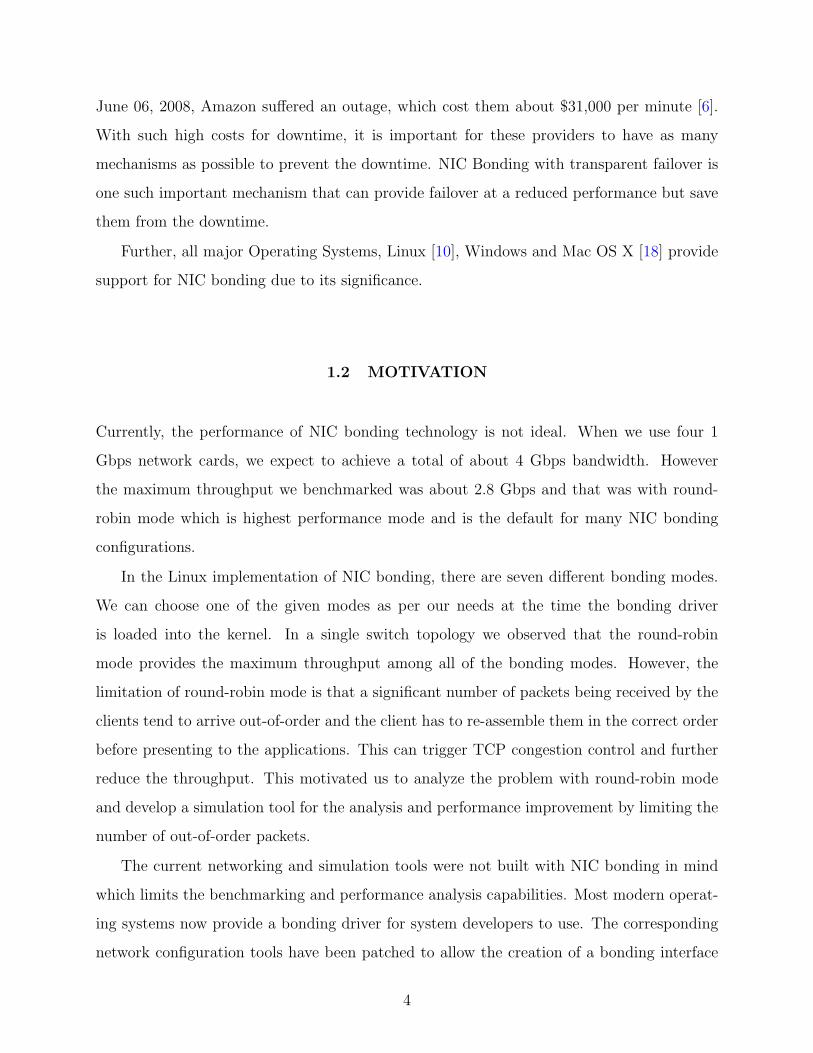
1.2 MOTIVATION

Currently, the performance of NIC bonding technology is not ideal. When we use four 1

Gbps network cards, we expect to achieve a total of about 4 Gbps bandwidth. However

the maximum throughput we benchmarked was about 2.8 Gbps and that was with round-

robin mode which is highest performance mode and is the default for many NIC bonding

configurations.

In the Linux implementation of NIC bonding, there are seven different bonding modes.

We can choose one of the given modes as per our needs at the time the bonding driver

is loaded into the kernel. In a single switch topology we observed that the round-robin

mode provides the maximum throughput among all of the bonding modes. However, the

limitation of round-robin mode is that a significant number of packets being received by the

clients tend to arrive out-of-order and the client has to re-assemble them in the correct order

before presenting to the applications. This can trigger TCP congestion control and further

reduce the throughput. This motivated us to analyze the problem with round-robin mode

and develop a simulation tool for the analysis and performance improvement by limiting the

number of out-of-order packets.

The current networking and simulation tools were not built with NIC bonding in mind

which limits the benchmarking and performance analysis capabilities. Most modern operat-

ing systems now provide a bonding driver for system developers to use. The corresponding

network configuration tools have been patched to allow the creation of a bonding interface

4

and the driver allows the integration of multiple network interfaces into a bond interface.

However, we found that the network analysis and simulation tools lacked support to study

NIC Bonding.

In this thesis work, we study the bonding modes, the bonding driver in the Linux ker-

nel and smart switch configuration to allow bonding/trunking. This was followed with a

performance analysis of existing bonding technology. To help us move beyond the current

state of technology, we developed a highly configurable bonding simulation tool. This tool

allowed us to analyze and develop new scheduling algorithms and study existing ones. We

developed a load-based scheduling algorithm as a solution for the out-of-order packets seen

by round-robin scheduling between the bonded interfaces.

1.3 THESIS ORGANIZATION

In the following chapters, we will start with a survey of commonly used NIC Bonding modes

[Chapter 2]. This will be followed by our experimental setup and configuration and a high-

level study of the bonding loadable kernel module in the Linux kernel [Chapter 3]. That

is followed by our bandwidth measurement results from our experiments with the available

bonding modes using existing tools and resources [Chapter 4]. Then we describe the design of

our simulation framework and its implementation [Chapter 5]. This is followed by simulation

usage and results in Chapter 6. Finally, we conclude with our contributions and ideas for

future work in Chapter 7.

5

2.0 BACKGROUND

Bonding of network interface cards allows for a number of possible use cases. For example,

we can simply distribute packets between the interfaces to make them look like a single

interface with the bandwidth that is the sum of the individual interfaces comprising the

bond. In another scenario, we can send packets on half of the interfaces and use the other

half for a transparent failover in case one of the active network interfaces fail. These and

similar functions are built into the bonding driver of the operating system and are known

as bonding modes. In the rest of this chapters, we’ll discuss these bonding modes and then

follow that with a discussion on the tradeoffs between them.

2.1 NIC BONDING MODES

As discussed in chapter 1, the bonding driver is part of the operating system kernel and

serves to combine a number of network interfaces into a single interface called a bond. The

individual network interfaces act as slaves of the bond interface allowing it to control the

packets that will be scheduled on them. The bond interface looks like a typical network

interface to user applications. This single interface will have unique properties that the

bonding driver enables using bonding modes. In each mode the application will see the

benefits of the bonding mode without having to worry about the actual implementation

details. Next, we will discuss the commonly used bonding modes provided by the current

operating system drivers.

6

2.1.1 Balanced-Round Robin

This is the default mode used by the bonding drivers on all operating systems that were

examined throughout this survey and experimentation. In this mode, if there are M incoming

packets, the scheduler distributes them among N network interfaces in a sequential order such

that each interface sends about the same number of packets. For example, if there are 6

incoming packets (p1-p6) and 4 interfaces (if1-if4) then p1 goes to if1, p2 to if2, p3 to if3,

p4 to if4, then p5 goes to if1, p6 to if2 and so on. This mode also provides fault tolerance

by dividing the packets among available interfaces. So if one of the interfaces is down or

unavailable, the incoming packets will get scheduled on the remaining interfaces allowing

the bonded interface to continue to work with reduced bandwidth. This allows for graceful

degradation of performance while maintaining a good load balance. The ingress for the

bonding driver is dependent on the switch/router that is being used (see: Experimental

Setup section 4.1). Round robin is easy to implement and use.

2.1.2 Active Backup

In this mode, only one slave interface is active at any given time. All slave interfaces are

assigned the same MAC address. The bond interface uses this common address as its own

MAC address. The other slaves in the bond serve as backups in the event the active interface

fails or becomes unreliable. If the active slave interface fails, the failure is detected by the

bonding driver and a backup slave interface is chosen to take over as the active slave interface.

The switch will effectively view this as the same interface that was disconnected from one

port and then connected to another port. This mode provides reliable fault tolerance but

does not provide any performance benefits. It is important to test the backup interface

from time to time. The bonding driver can switch the transmission to a backup interface

occasionally to test it. In Linux, the driver periodically switches between the available slaves

making each of them active for a fixed period. So, every 100ms or so, one of the backup

interfaces is chosen to be the active interface until the next time slot. Then the second

backup becomes active and so on.

This mode is preferred for deployments where high availability of the network interface is

7

critical. Examples of such deployments are real-time systems running life-critical applications

and high availability websites.

2.1.3 Balanced-XOR

In Balance-XOR mode the slave interface to be used for transmission of a packet is chosen

by calculating the XOR of the MAC addresses of the host and the destination:

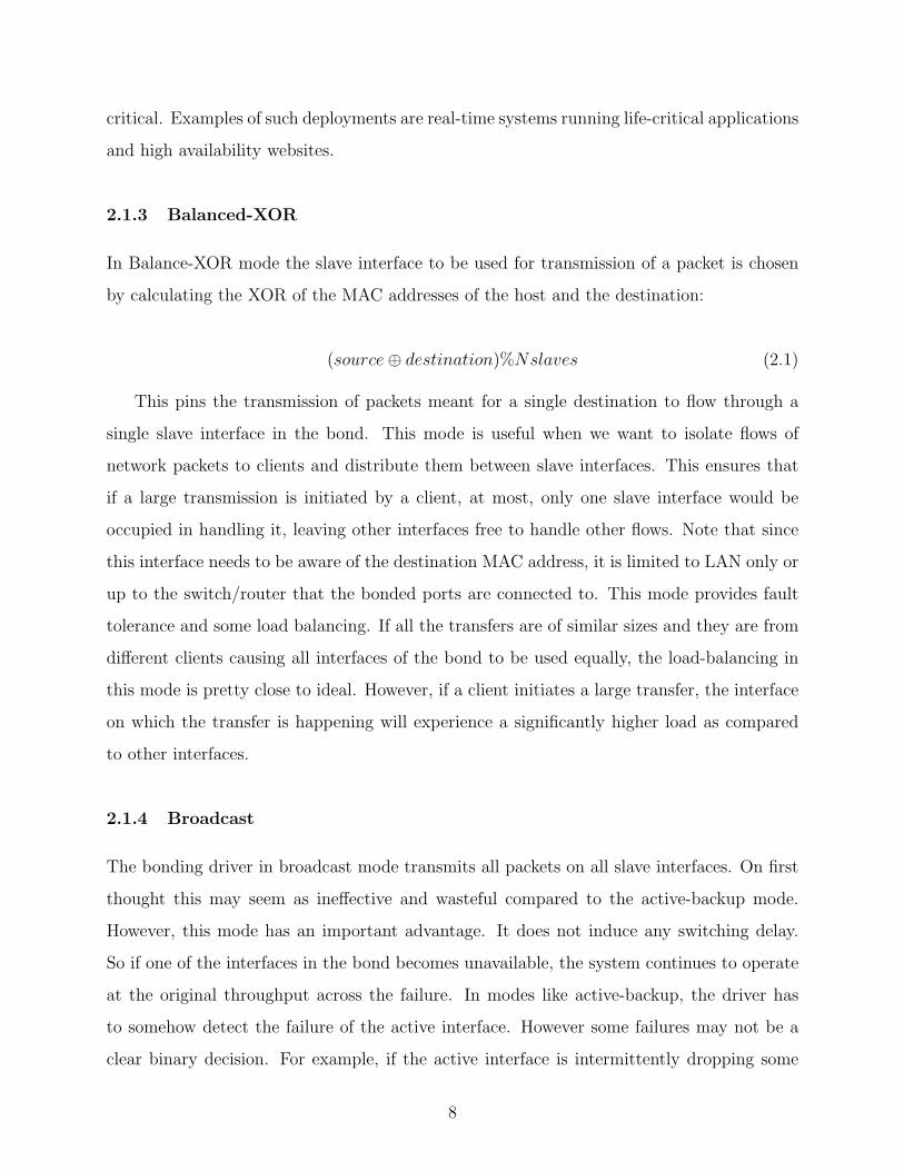
(source⊕ destination)%Nslaves (2.1)

This pins the transmission of packets meant for a single destination to flow through a

single slave interface in the bond. This mode is useful when we want to isolate flows of

network packets to clients and distribute them between slave interfaces. This ensures that

if a large transmission is initiated by a client, at most, only one slave interface would be

occupied in handling it, leaving other interfaces free to handle other flows. Note that since

this interface needs to be aware of the destination MAC address, it is limited to LAN only or

up to the switch/router that the bonded ports are connected to. This mode provides fault

tolerance and some load balancing. If all the transfers are of similar sizes and they are from

different clients causing all interfaces of the bond to be used equally, the load-balancing in

this mode is pretty close to ideal. However, if a client initiates a large transfer, the interface

on which the transfer is happening will experience a significantly higher load as compared

to other interfaces.

2.1.4 Broadcast

The bonding driver in broadcast mode transmits all packets on all slave interfaces. On first

thought this may seem as ineffective and wasteful compared to the active-backup mode.

However, this mode has an important advantage. It does not induce any switching delay.

So if one of the interfaces in the bond becomes unavailable, the system continues to operate

at the original throughput across the failure. In modes like active-backup, the driver has

to somehow detect the failure of the active interface. However some failures may not be a

clear binary decision. For example, if the active interface is intermittently dropping some

8

packets, the active-backup mode driver code may not detect such a situation. However, with

Broadcast mode, since all slaves are transmitting, even if one of them manages to send the

packet, the destination sees no delay. The switch or destination host can simply drop the

extra transmitted packets using the TCP sequence number. This mode does not provide any

load balancing but provides zero-delay fault tolerance as long as one of the slave interfaces

is functioning. However, in spite of the above mentioned advantages, the broadcast mode

has a detrimental effect in terms of network resource utilization. All the additional packets

have to be processed by the network switches and this significantly reduces the goodput of

the network.

2.1.5 802.3ad

IEEE 802.3ad or Dynamic link aggregation mode implements the Link Aggregation Control

Protocol (LACP). This allows a network device to negotiate an automatic bundling of several

physical interfaces to form a single logical channel with a peer that also implements LACP.

LACP works by sending frames (LACPDUs) down all links that have the protocol enabled.

If it finds a device on the other end of the link that also has LACP enabled, it will also

independently send frames along the same links enabling the two units to detect multiple

links between themselves and then combine them into a single logical link. This creates

aggregation groups that share the same speed and duplex settings. This mode utilizes all

slaves in the active aggregator according to the 802.3ad specification. It is highly effective

but requires configuration changes on the switch and the switch must support 802.3ad Link

Aggregation.

2.1.6 Balance - TLB

Transmit load balancing mode allows channel bonding that does not require special switch

support like the 802.3ad mode. The outgoing traffic is distributed according to the current

load (computed relative to the speed) on each slave. The outgoing packets are assigned to

interfaces after calculating the relative speed of each interface using ethtool. The speeds are

calculated in real-time while scheduling packets. So, the slower interfaces get lesser packets.

9

For example, if one of the interfaces is transmitting 10% slower, it will have 10% fewer

packets queued to it. Among the interfaces that are running at the same speed the packets

are sent sequentially similar to the round-robin mode. For the incoming traffic, the driver

assigns one of the interfaces as the current slave. This is the interface that receives all of the

incoming traffic. If the receiving slave fails, another slave takes over the MAC address of

the failed receiving slave. This mode provides fault tolerance and transmit (outgoing) load

balancing. It provides no receiving load balancing.

2.1.7 Balance - ALB

In Balance-ALB mode adaptive load balancing is bidirectional. In addition to the transmit

load balancing provided by the Balance-TLB mode, this mode provides receive load balancing

of IPV4 traffic by distributing incoming traffic among all slave interfaces belonging to the

bond. The receive load balancing is achieved by ARP negotiation. When the client machines

need to connect to the server, they send an ARP request to find the server’s MAC address.

The bonding driver intercepts the ARP Replies sent by the server system1 on their way out to

the requesting client and overwrites the source hardware address with the unique hardware

address of one of the slaves in the bond such that different clients use different hardware

addresses for connecting to the server. Thus, for incoming packets, all packets arriving

from one client arrive on one slave interface. This allows different slave interfaces to receive

packets from different clients allowing for load-balancing, whereas in case of Balance-TLB,

all packets were received by a single slave interface.

The summary of all the bonding modes is given in Table 1.

2.2 TRADEOFFS

As we noticed in the previous section [2.1], all of these bonding modes have a number of

tradeoffs that the network administrator needs to consider before selecting one of these

1The system on which the bonding interface is set-up

10

Table 1: Comparison of Bonding modes

BondingMode Properties

Balanced

Round Robin

Transmit packets in sequential order to all slave in-

terfaces

Active Backup Only one slave in the bond is active

Balanced-XOR Same slave for each destination MAC address.

Broadcast Transmit all packets on all slave interfaces.

802.3adCreates aggregation group of slaves that share same

speed and duplex setting.

Balanced TLB Traffic distributed based on speed of each interface.

Balance ALB Includes balance TLB plus Receive load balancing.

modes.

To begin with, the choice of a bonding mode needs to be made when the bonding driver

is loaded. The bonding mode cannot be changed without turning off the bond interface and

re-loading the bonding driver.

An undesirable side effect of round robin scheduling is that the packets can arrive out-

of-order. This results in lower than expected bandwidth due to the reordering and caching

overhead. As packets are transmitted using round-robin scheduling, some interfaces may have

their transmission queues build up causing all of the packets on those interfaces to arrive

out of order. For example, on a system with four network interface cards, if few interfaces

are running slower and clients did not receive packets on time, TCP/IP’s congestion control

system will kick in. After three duplicate ACKs, interfaces will have to retransmit the

segment and TCP will cut down the window size to the half of its original. This will reduce

the bandwidth significantly.

With XOR mode, if the number of clients communicating with the bond is large and

their MAC addresses are randomly distributed, there is good load balancing between flows

to each of the clients. However, it loses effectiveness as the number of connecting hosts

decreases and is in the same order as the number of interfaces.

The 802.3ad mode requires the network switch and routers to be aware of link aggregation

control protocol. Thus the use of this mode increases the initial setup cost for the network.

11

The TLB and ALB modes depend on ethtool to obtain the speed of the slave network

interfaces and base their scheduling on that. This does not account for changing load due

to differences in timing or outside network activity such as congestion.

In summary, it is a difficult choice for the network administrator to choose between one

of these modes, which is made more difficult with the fact that changing the choice would

require disabling the bond and reloading the bonding driver with the new bonding mode

enabled.

12

3.0 BONDING IN LINUX KERNEL

To further understand the internals of how bonding is implemented, we looked at the actual

implementation of the bonding driver on Linux. Even though bonding is supported on all

major operating systems, we chose Linux because of driver source code availability. In this

chapter, we start with a high-level overview of how bonding is implemented as a driver for the

Linux kernel. This is followed by a description of our experimental setup and configuration

that was used for measurements and analysis.

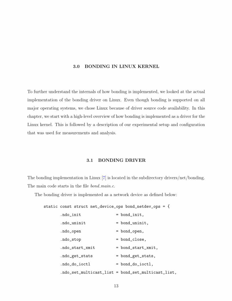
3.1 BONDING DRIVER

The bonding implementation in Linux [7] is located in the subdirectory drivers/net/bonding.

The main code starts in the file bond main.c.

The bonding driver is implemented as a network device as defined below:

static const struct net_device_ops bond_netdev_ops = {

.ndo_init = bond_init,

.ndo_uninit = bond_uninit,

.ndo_open = bond_open,

.ndo_stop = bond_close,

.ndo_start_xmit = bond_start_xmit,

.ndo_get_stats = bond_get_stats,

.ndo_do_ioctl = bond_do_ioctl,

.ndo_set_multicast_list = bond_set_multicast_list,

13

.ndo_change_mtu = bond_change_mtu,

.ndo_set_mac_address = bond_set_mac_address,

.ndo_neigh_setup = bond_neigh_setup,

.ndo_vlan_rx_register = bond_vlan_rx_register,

.ndo_vlan_rx_add_vid = bond_vlan_rx_add_vid,

.ndo_vlan_rx_kill_vid = bond_vlan_rx_kill_vid,

};

So bond init is where the driver code starts. It initializes a single work queue as a

synchronization point for the requests before they are distributed between slaves:

bond->wq = create_singlethread_workqueue(bond_dev->name);

After the initialization, the driver waits for bond create() which causes the creation of a

bond interface. After that bond open() will be called to handle the bonding mode and other

option selection from the network administrator. This point onwards, bond get stats() can

be called to retrieve bond statistics.

Once the initial device is set up, the user calls the ioctl interface to call bond do ioctl()

in the driver code. This is how bonding specific arguments and actions are initiated by the

user tools such as ifconfig. Depending on the ioctl() command, the action may be one of

bond enslave(), bond release(), bond sethwaddr() and bond ioctl change active() to enslave

an interface card, release the interface card from the bond, set the hardware address of the

bonding interface and to change the active interface for the bond respectively.

The transmission hash policy is defined by one of bond xmit hash policy 123(),

bond xmit hash policy 134() or bond xmit hash policy 12() as follows:

return (data->h_dest[5] ^ data->h_source[5]) % count;

So, as discussed in section 2.1, the slave chosen for the transmission is calculated using an

XOR between the source and destination addresses modulus the number of slaves in the

bond. The numbers in those function names represent the OSI layers depending on which

the calculation is made.

The actual transmission is started by bond start xmit() which in turn invokes the mode

specific transmission function:

14

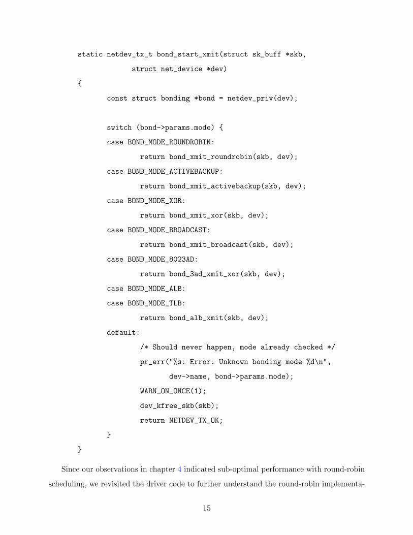
static netdev_tx_t bond_start_xmit(struct sk_buff *skb,

struct net_device *dev)

{

const struct bonding *bond = netdev_priv(dev);

switch (bond->params.mode) {

case BOND_MODE_ROUNDROBIN:

return bond_xmit_roundrobin(skb, dev);

case BOND_MODE_ACTIVEBACKUP:

return bond_xmit_activebackup(skb, dev);

case BOND_MODE_XOR:

return bond_xmit_xor(skb, dev);

case BOND_MODE_BROADCAST:

return bond_xmit_broadcast(skb, dev);

case BOND_MODE_8023AD:

return bond_3ad_xmit_xor(skb, dev);

case BOND_MODE_ALB:

case BOND_MODE_TLB:

return bond_alb_xmit(skb, dev);

default:

/* Should never happen, mode already checked */

pr_err("%s: Error: Unknown bonding mode %d\n",

dev->name, bond->params.mode);

WARN_ON_ONCE(1);

dev_kfree_skb(skb);

return NETDEV_TX_OK;

}

}

Since our observations in chapter 4 indicated sub-optimal performance with round-robin

scheduling, we revisited the driver code to further understand the round-robin implementa-

15

tion. The corresponding code is in bond xmit roundrobin():

slave_no = bond->rr_tx_counter++ % bond->slave_cnt;

bond_for_each_slave(bond, slave, i) {

slave_no--;

if (slave_no < 0)

break;

}

start_at = slave;

bond_for_each_slave_from(bond, slave, i, start_at) {

if (IS_UP(slave->dev) &&

(slave->link == BOND_LINK_UP) &&

(slave->state == BOND_STATE_ACTIVE)) {

res=bond_dev_queue_xmit(bond,skb,slave->dev);

break;

}

}

This implementation cycles through each slave and transmits a packet from the bond inter-

face queue using bond dev queue xmit(). This is a very simple and naıve approach which

does not account for load on the slave interface.

3.2 BONDING CONFIGURATION ON LINUX

To configure bonding, we need to create a bonded interface using the bonding driver. Once

the interface is configured, we use a tool called ifenslave to make physical interfaces act

as slaves of the bonded interface. We start the configuration by taking down all network

16

interfaces that will act as slaves:

sudo ifdown eth1 eth2 eth3 eth4

Then loaded the bonding module into the Linux kernel

modprobe bonding

There are two important options to pass to the module: mode and miimon. The default

mode is round-robin but others can be chosen (backup, XOR, broadcast, 802.3ad, TLB,

ALB). Miimon establishes how often (in milliseconds) the links will be checked for failure.

A value of zero disables link monitoring.

For example, the following command will set up a round robin configuration in which

network packets alternate between the network interfaces as they are sent out.

modprobe bonding mode = 0 miimon = 100

After the module is loaded into the kernel, a bonding interface can be created as follows:

ifconfig bond0 <ipaddr> netmask <netmask> up

Once the bond0 interface was created, the network interface cards can be enslaved to it.

ifenslave bond0 eth1 eth2 eth3 eth4

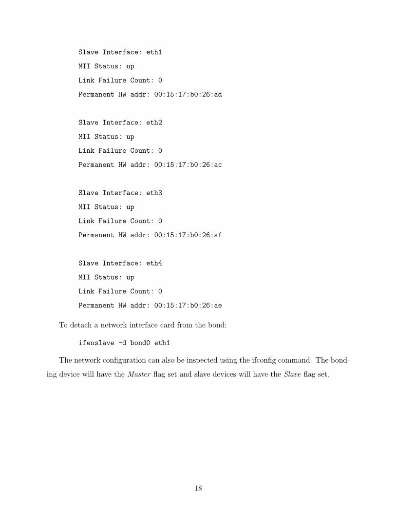
Information about a bonding interface can be obtained from /proc/net/bonding/bond0.

Here is an example after the driver was loaded with mode = 0 (round-robin) and miimon =

100 is as follows:

cat /proc/net/bonding/bond0

Ethernet Channel Bonding Driver: v3.3.0 (June 10, 2008)

Bonding Mode: load balancing (round-robin)

MII Status: up

MII Polling Interval (ms): 100

Up Delay (ms): 0

Down Delay (ms): 0

17

Slave Interface: eth1

MII Status: up

Link Failure Count: 0

Permanent HW addr: 00:15:17:b0:26:ad


MII Status: up


Permanent HW addr: 00:15:17:b0:26:ac


MII Status: up


Permanent HW addr: 00:15:17:b0:26:af


MII Status: up


Permanent HW addr: 00:15:17:b0:26:ae

To detach a network interface card from the bond:

ifenslave -d bond0 eth1

The network configuration can also be inspected using the ifconfig command. The bond-

ing device will have the Master flag set and slave devices will have the Slave flag set.

18

4.0 THROUGHPUT MEASUREMENT

To find out the performance differences between various bonding modes and know which

mode gives better throughput under the given conditions, we ran some experiments. We

used various network testing tools such as iperf, httperf and zipf to measure the performance

of bonding with different modes.

4.1 EXPERIMENTAL SETUP

We used a 4-port NIC card using Intel Corporation 82571EB ethernet controller on machine

X (Server) with the four ports connected to a Netgear GS724TR smart switch. In addition,

there were four physical client machines (A, B, C, D), also connected to the switch as shown

in figure 2. The switch has a maximum bandwidth of 1 Gbps per port and 4 Gbps for a link

aggregation group (LAG). A LAG is configured using the management interface of the switch

and serves as a mechanism to combine connections on multiple ports into an aggregation

group. Setting up a LAG informs the switch that the ports belonging to it will be using NIC

bonding.

4.2 SWITCH CONFIGURATION

The network switches can be built to support NIC bonding. These switches have to be aware

that the physical interfaces connected to a set of ports belong to a bond and are effectively

connected to a single machine that treats them as an individual interface. This allows the

19

Server X SwitchClient B

Client A

Client C

Client D

eth 1

eth 2

eth 3

eth 4

Port 1

Port 2

Port 3

Port 4

Port 5

Port 8

Port 7

Port 6

Figure 2: Switch setup

switch to accept the fact that all of those interfaces will advertise their MAC address as the

same and allows it to handle the ARP tables accurately. The switch level implementation is

called trunking or aggregation.

We configured bonding/trunking on a Netgear GS724TR switch. On the management

interface of the switch, under the port configuration section, we configured the physical

interfaces connected to ports corresponding to the four ports from the quad-port NIC card

on machine X under a Link aggregation group (LAG). This informs the switch that the four

interfaces are part of a bond and should be treated as such. Since the switch has a maximum

bandwidth of 4 Gbps, it should now be possible to transmit at that rate from machine X

to the four client machines A, B, C and D. After this configuration, the Netgear switch

indicated that four ports were now functioning as a common trunk. Ports g1, g2, g3 and g4

became members of LAG 1.

4.3 MEASUREMENTS

Initially we used iperf to check if the bonding is working properly. We ran iperf on the server

and it started listening on a specific port. Then we sent 1 GB data from all four clients

to the server and measured the bandwidth. We got around 830 Mbps for each client (total

of 3320 Mbps) in case of balanced round-robin. It showed us that the bonding has been

20

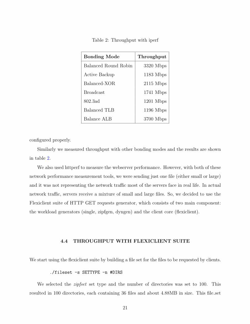
Table 2: Throughput with iperf

Bonding Mode Throughput

Balanced Round Robin 3320 Mbps

Active Backup 1183 Mbps

Balanced-XOR 2115 Mbps

Broadcast 1741 Mbps

802.3ad 1201 Mbps

Balanced TLB 1196 Mbps

Balance ALB 3700 Mbps

configured properly.

Similarly we measured throughput with other bonding modes and the results are shown

in table 2.

We also used httperf to measure the webserver performance. However, with both of these

network performance measurement tools, we were sending just one file (either small or large)

and it was not representing the network traffic most of the servers face in real life. In actual

network traffic, servers receive a mixture of small and large files. So, we decided to use the

Flexiclient suite of HTTP GET requests generator, which consists of two main component:

the workload generators (single, zipfgen, dyngen) and the client core (flexiclient).

4.4 THROUGHPUT WITH FLEXICLIENT SUITE

We start using the flexiclient suite by building a file set for the files to be requested by clients.

./fileset -s SETTYPE -n #DIRS

We selected the zipfset set type and the number of directories was set to 100. This

resulted in 100 directories, each containing 36 files and about 4.88MB in size. This file set

21

was then copied to the http server directory for serving HTTP GET requests from clients.

We used the nginx HTTP server for this purpose because it is very lightweight and built for

performance.

Then the zipfgen workload generator was used to generate SPECWeb99-like static re-

quests in the format of ./file set/dir/XXXXX/classY Z. The workload generator has the

following command

./zipfgen -s <set> -n <size> -active <#simultaneous_req> -a <Zipf alpha>

Where, set is the target set (spec—deg), size is the number of directories or files, active

is the number of simultaneous outstanding requests. We used the following command to

generate our file set:

./zipfgen -s spec -n 20 -active 64 -a 50

The requests generated by zipfgen were then sent to the flexiclient. When started, the

flexiclient will listen on port 7979 (by default) and wait for the trigger signal from the

clientmaster. One flexiclient is run on each client machine. Then when the clientmaster is

ready it will signal all flexiclient instances to send their GET requests to the HTTP server.

The flexiclient is invoked on each client as follows:

./flexiclient -host <srv_addr> -port <srv_port> -time <sec> -active <#simultaneous_req>

After the flexiclient instances send their requests and receive responses from the HTTP

server, they print their statistics on the console. These statistics were collected and analyzed

for our experiments.

4.4.1 Throughput without bonding

Initially, we measured the throughput without bonding on all four interfaces of the server

and only one client sent the HTTP requests for different files. We measured the throughput

and got about 723.2 Mbps. Even with a single NIC if there are requests for a number of files

the throughput is decreased as compared to the request of a single file in case of iperf and

httperf.

./zipfgen -s spec -n 10 -active 64| ./flexiclient -host

22

130.49.223.244 -port 8000 -time 30

# avgspeed time totbytes xactbytes reqs byt/req conns # fHeadT fBodyT lBodyT

#[ 723.2 30 2711843615 2711873258 179383 15117.6 179399 0 0 1 ]

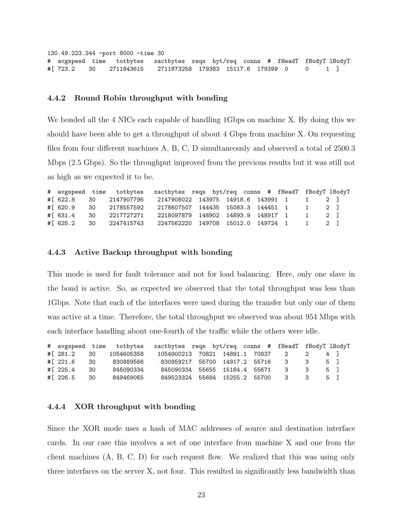
4.4.2 Round Robin throughput with bonding

We bonded all the 4 NICs each capable of handling 1Gbps on machine X. By doing this we

should have been able to get a throughput of about 4 Gbps from machine X. On requesting

files from four different machines A, B, C, D simultaneously and observed a total of 2500.3

Mbps (2.5 Gbps). So the throughput improved from the previous results but it was still not

as high as we expected it to be.


#[ 622.8 30 2147907796 2147908022 143975 14918.6 143991 1 1 2 ]

#[ 620.9 30 2178557592 2178607507 144435 15083.3 144451 1 1 2 ]

#[ 631.4 30 2217727271 2218097879 148902 14893.9 148917 1 1 2 ]

#[ 625.2 30 2247415743 2247562220 149708 15012.0 149724 1 1 2 ]

4.4.3 Active Backup throughput with bonding

This mode is used for fault tolerance and not for load balancing. Here, only one slave in

the bond is active. So, as expected we observed that the total throughput was less than

1Gbps. Note that each of the interfaces were used during the transfer but only one of them

was active at a time. Therefore, the total throughput we observed was about 954 Mbps with

each interface handling about one-fourth of the traffic while the others were idle.


#[ 281.2 30 1054605358 1054900213 70821 14891.1 70837 2 2 4 ]

#[ 221.6 30 830889566 830959217 55700 14917.2 55716 3 3 5 ]

#[ 225.4 30 845090334 845090334 55655 15184.4 55671 3 3 5 ]

#[ 226.5 30 849469065 849523324 55684 15255.2 55700 3 3 5 ]

4.4.4 XOR throughput with bonding

Since the XOR mode uses a hash of MAC addresses of source and destination interface

cards. In our case this involves a set of one interface from machine X and one from the

client machines (A, B, C, D) for each request flow. We realized that this was using only

three interfaces on the server X, not four. This resulted in significantly less bandwidth than

23

we expected. On manually calculating the hash of MAC addresses, we realized that flows

to two machines were hashing to the same value resulting in one interface staying idle. To

rectify this problem we changed the mac address and started to use both layer 3 and layer 4

to calculate hash by adding the following option when loading the bonding kernel module:

xmit_hash_policy=layer3+4

After this, XOR mode started using all four interfaces and the throughput improved

as compared to the previous experiments. With this workaround, we achieved about 2400

Mbps.


#[ 541.2 30 1593728071 1594632764 106184 15009.1 106200 2 2 3 ]

#[ 466.2 30 1748163857 1748169877 114929 15210.8 114945 2 2 3 ]

#[ 696.9 30 2613424248 2614198849 173706 15045.1 173722 1 1 2 ]

#[ 695.9 30 2609710150 2609783689 175616 14860.3 175631 1 1 2 ]

4.4.5 Broadcast throughput with bonding

Broadcast is not used for load balancing It will just transmit everything on all slave interfaces.

In this mode we were able to observe a throughput of only about 486.5 Mbps. This seems

lower than expected but it should be noted that the additional broadcast traffic will cause

collisions and hence cause even further reduced throughput.


#[ 117.8 30 441580268 442112060 28823 15320.4 28839 0 0 6 ]

#[ 118.4 30 444075391 444806551 27910 15911.0 27926 0 0 7 ]

#[ 122.5 30 459504921 460288893 30193 15218.9 30209 0 0 6 ]

#[ 127.8 30 479150119 480292742 32460 14761.2 32476 0 0 5 ]

4.4.6 802.3ad throughput with bonding

Similar to the XOR mode, this mode also uses the hash of source and destination MAC

addresses to distribute load among the network interface cards. We were able to use the

same workaround as in section 4.4.4. After the workaround we were able to get a total of

982 Mbps.


#[ 231.1 30 866522562 866555328 60143 14407.7 60159 3 3 5 ]

#[ 229.7 30 861418311 861768956 57581 14960.1 57597 3 3 5 ]

24

#[ 252.0 30 944888777 945038832 63640 14847.4 63656 3 3 4 ]

#[ 269.2 30 1009442153 1009468672 66746 15123.6 66762 3 3 5 ]

4.4.7 TLB throughput with bonding

In this mode the outgoing traffic is distributed according to the current load on each client.

Since the load was distributed fairly evenly we were able to get a total of 1750.0 Mbps.


#[ 467.5 30 1753126807 1753670180 118396 14807.3 118411 3 3 3 ]

#[ 424.1 30 1590405798 1590408922 106358 14953.3 106374 3 3 3 ]

#[ 428.7 30 1585252665 1585455841 106274 14916.7 106290 3 3 3 ]

#[ 429.7 30 1611282263 1611282263 108533 14846.0 108549 3 3 3 ]

4.4.8 ALB throughput with bonding

As with the TLB mode, the outgoing traffic was distributed well and we were able to got a

total of 2140.5 Mbps.


#[ 575.5 30 2158253209 2158274390 144497 14936.3 144513 2 2 2 ]

#[ 497.8 30 2279398304 2279601936 149383 15258.8 149399 2 2 2 ]

#[ 579.3 30 2172421904 2173003465 144646 15018.9 144661 2 2 2 ]

#[ 487.9 30 2485723478 2485723478 164238 15134.9 164254 2 2 2 ]

4.4.9 Bonding throughput summary

As we had expected, the throughput varied a lot with different bonding modes as shown in

figure 3. The maximum throughput that we observed was 2.5 Gbps with round-robin mode.

This is far less than the ideal expected throughput of 4 Gbps. So we decided to study the

round-robin performance in detail and identify approaches that would help in achieving a

higher throughput

Our analysis of the performance of round-robin was hindered by the lack of proper

analysis and simulation tools for bonding. So we decided to simulate the entire setup using

a highly configurable simulation framework that would serve as a testbed for our further

experiments.

25

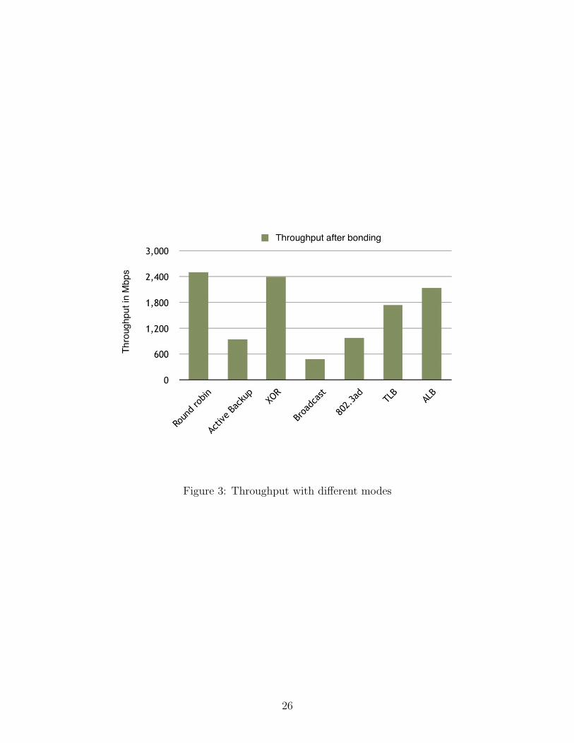
Figure 3: Throughput with different modes

26

5.0 BONDING SIMULATOR

A new bonding simulator was developed to further the research effort in improving the max-

imum throughput of NIC bonding. This tool is called bondingSimulator and was designed

from scratch to be highly configurable and adaptable with minimal effort. It was necessary

to design and develop this tool because the existing network simulation tools do not provide

good support for simulating alternate implementations of the NIC bonding logic.

5.1 KEY FEATURES

The key objective of our research was to analyze and improve the performance of round-robin

scheduling algorithm by reducing the number of out-of-order packets. The bondingSimulator

played a key role by allowing us to implement round-robin and our proposed solution, load-

based scheduling side-by-side and compare the performance of the two algorithms without

having to write complicated kernel code.

The bondingSimulator allows researchers and network engineers to study the effect of NIC

bonding at various levels. Everything from the number of clients, number of simultaneous

requests, the size of requests, the scheduling algorithm, the speed and order of interface

operation and timing is configurable. The tool also provides a number of post-processing

scripts that allow the user to develop aggregate statistics from raw data and even plot these

observations on to visual graphs.

Since it is difficult to predict the research uses of such a tool and the needs of future users,

the tool was implemented using object-oriented models to keep all components highly mod-

ular and independent. The bondingSimulator uses asynchronous programming paradigms

27

Switch

Client 0

Client 1

Client 2

Client 3

Client 4

Client 5

Bond OS

App 1IF 0

IF 1

IF 2

IF 3

App 2

App 3

App 4

Server

Figure 4: Basic experimental setup

to further simplify the implementation and provide a tight control over the various com-

ponents without having to worry about multithreaded complications and locking between

tools. This also makes it realistic because most real-world components in a bonding setup

work asynchronously.

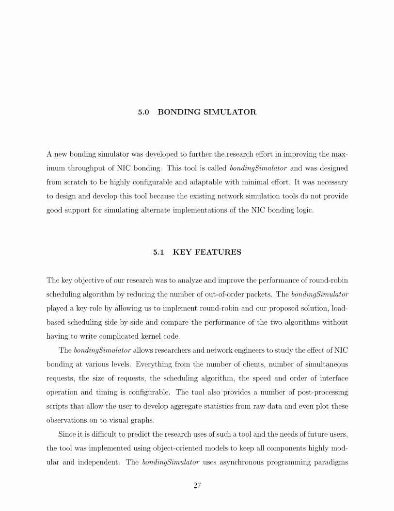
5.2 DESIGN

The bondingSimulator builds on top of the model for our experimental setup discussed in

section 4.1. As shown in figure 4, the bondingSimulator is designed to simulate a number of

clients connected to the bonded interfaces on the server through a high-performance bonding-

aware switch. The server combines the slave interfaces into a single bonded interface as seen

by the operating system and applications. The clients request files from a HTTP daemon

running on the server. The HTTP daemon binds to the bonded interface and serves these

requests by reading files off the storage device (local disk or network attached).

After careful analysis we realized that all of the components did not have to be actually

28

simulated. For example, since the requests are quite similar in nature and form they need

not necessarily come from the clients so we designed a requestGenerator to generate these

requests. This allows the requestGenerator to be a single component that controls how

the requests are formed and generated. Another such component is the switch. Since the

switching of packets between components happens in memory in the simulator, it was not

necessary to build it as a separate component.

...... R4 R3 R2 R1Request

Generator

Request Queue

Scheduler

IF 0 .. .. ...

IF n .. .. ...

IF 1 .. .. ... ..

Queue Packets

Client 0 .. .. ...

Client n .. .. ...

Client 1 .. .. ... ..

Switching

Server

Simulation Log

Average & Probability Statistics

Plot visual graphs for

comparison

process.sh plot.sh

Final Processing

Figure 5: Bonding Simulator Design

The bondingSimulator simulates four different kinds of components: requestGenerator,

scheduler, interfaces and clients as shown in figure 5. It was not necessary to implement

applications on clients and servers but those can be easily implemented by extending the

scheduler and client components.

29

The requestGenerator simulates incoming requests from the clients. It randomly gener-

ates these requests for files that are known to exist on the server’s storage. Each request

is simulated to come from one of the clients in the simulation. The number of clients is

configurable. These requests are queued into the requestQueue.

The scheduler periodically reads the requestQueue. The scheduler reads the requested

file and queues up packets from the file among the available interfaces depending on the

user-selected bonding mode. There can be a number of simultaneous outstanding requests

and the policy on how many of them should be handled in a given time slot is configurable.

At the end of the simulation, the scheduler detects the end of simulation due to lack of

incoming requests and causes all components to do their post-simulation processing after

waiting for their work queues to be exhausted.

All interfaces share a common code base. Each interface accepts incoming packets from

the scheduler. All interfaces run independently of each other and process the pending packets

in their queue. These packets are sent to the respective clients that requested the file that

the chunks belong to. Since each client requests files independently it is possible that a client

is receiving more than one file at any given time from one or more interfaces.

The clients in-turn receive packets containing file chunks from the interfaces. These pack-

ets are processed as they are received. Our current implementation is focused on identifying

out of order packets but can be adapted to handle other kinds of analysis.

5.3 IMPLEMENTATION

The entire simulation runs as a single process using asynchronous programming. This allows

us to avoid the multi-threading peculiarities such as thread switching and synchronization

that can adversely affect the simulation results. Python Twisted asynchronous programming

was used for this simulation. It is based on a UNIX select() loop to handle the event-driven

programming model. The simulation starts at the bondingSimulator module, by parsing

the user options, setting up the interfaces, clients, scheduler and requestGenerator objects

and starting each object’s event loop. The simulation ends when all requests generated

30

randomly by the requestGenerator have been handled and all file chunks have been received

at the respective clients. For networking and processing delays we have used random intervals

but the simulator can be easily adapted to work using traces collected from live systems. In

the rest of this section we will describe each component in more detail.

5.3.1 Bonding simulator

The bondingSimulator class is the main class that interfaces with the user and is used to

initiate the simulation based on the user’s inputs. The code starts with the creation of a

Parser object to handle user-provided options. The arguments are validated and passed on

to the bondingSimulator function. The bondingSimulator in turn uses the provided argu-

ments including file set, num clients, ifaces, requests and algorithm. It starts by creating a

requestGenerator object and initiating the generation of requests by calling its generate()

function.

This is followed by the creation of a client object for each client. So if n clients were

requested, there will be n client objects. References to these client objects are stored in a

list called client list. This list is a single object that can be passed to any other objects that

may wish to interact with the client objects.

After the creation of clients, the interface objects are created. As with clients, the number

of interfaces is user configurable using a command-line option. Each interface object is passed

a reference to the client list. This reference allows each interface to call the client to deliver

packets destined for that client. Once the interfaces are created, the bondingSimulator starts

their corresponding event handling loops. Initially, the interfaces would not have packets to

process in their queues, so the event loop would sit idle and it is safe to initiate it at this

time. References to the interface objects that were created are stored in the iface list.

Once the clients and interfaces are created, the scheduler is created. The scheduler needs

to be able to interact with all other components including the request generator, interfaces

and clients, so the corresponding references to the request generator, iface list and client list

are passed as arguments to its constructor.

Finally, the bondingSimulator calls reactor.run() to start the main control loop for the

31

simulation. This loop is what drives the individual event loops of all periodic components

such as request generator, scheduler, interfaces and clients. At this point the simulation is

fully operational.

5.3.2 Request generator

The requestGenerator is the first component created by the bondingSimulator . The re-

questGenerator module provides a class called request to create requestor objects. For our

simulation, we had only one requestor but more can be created if needed. The constructor

inputs include, file set, num clients and the number of total requests to be generated. The

object maintains a count of the total requests that have been generated so far.

The requestor has a main event loop called generate() that is used to periodically generate

requests. The generate() event loop calls random request() to generate a random request

within the constraints of the number of clients and the files in the file set. Each generated

request is printed on the console as a progress indicator for the user. Each such new request

is appended to the request queue. This is the data structure that the scheduler references

to identify the requests to be processed. Finally, the requestor updates the count of requests

generated so far and schedules the generate() event to fire after a fixed or random duration of

time. This duration of time is what determines how frequently the requests will be generated.

It is possible to generate more than one request in each iteration of the generate() call by

including a loop in that function as follows:

- if(self.requested >= self.num_requests):

- return

- request = self.random_request()

- print request

- self.request_queue.append(request)

- self.requested = self.requested + 1

- reactor.callLater(1, self.generate)

+ for i in range(1,1000):

+ if(self.requested >= self.num_requests):

32

+ return

+ request = self.random_request()

+ print request

+ self.request_queue.append(request)

+ self.requested = self.requested + 1

+ reactor.callLater(randint(1,5), self.generate)

Each request is generated randomly by the random request() function which in turn calls

random client name() and random file name() to pick a client randomly from the set of

client objects and a valid file name from the given file set.

It was a little tricky to generate a random file name because the target files are dis-

tributed in a large set of subdirectories and we wanted to randomize the requests over the

entire set of files. This was achieved by noting that the directory names follow a sequential

numbering and each directory contains the same set of file names albeit with different file

contents. The corresponding code to generate the random file name is:

file_name = (glob.glob("%s/dir%05d/class3_*" % \

(self.file_set, randint(10,num_dirs))))[0]

5.3.3 Scheduler

The scheduler is responsible for processing the requests generated by the request generator.

It reads the outstanding requests from the request queue, opens the requested files, reads

chunks of data from those files, forms these chunks into packets and queues them on to the

interfaces to be sent to the clients that requested them.

The scheduler is implemented as a class called schedule. The constructor for this class

takes the following arguments:

algo The scheduling algorithm to be used for distributing packets.

queue The request queue reference from requestGenerator .

iface list List of references to all interfaces.

33

client list List of references to all clients.

chunk size Chunk or packet payload size.

In addition to the arguments passed to the constructor, the scheduler object maintains

three other values. The next iface to be used when using round-robin scheduling, the next req

sequence number for the next request to be processed and a watchdog timer to time out and

end the simulation after no more incoming requests are detected. The detection of end-

of-simulation is necessary to flush out all interface and client queues and print out final

statistics. The constructor also initialzes two name-value pair dictionaries:

fd dict (request num, file descriptor) tuple dictionary.

file chunk (request num, file chunk) tuple dictionary.

These dictionaries allow the scheduler to keep track of open file descriptors for all requests

and chunk offset into each file that is currently being read.

After initialization, the scheduler’s event loop process() is started by the bondingSimula-

tor and it starts operating when the reactor.run() discussed in section 5.3.1 is called by the

bondingSimulator .

Like other components’ event loops, process() runs periodically and the period can be

controlled from the last line in that function:

# Done queuing all outstanding requests to interfaces

# Check for new requests after some time

reactor.callLater(0.030, self.process)

Schedule() starts with reading the outstanding requests in the request queue. As men-

tioned earlier, with asynchronous programming, since only one component can be running

at a time we don’t have to worry about the request queue being modified as the scheduler

reads it. Each request names a file that the client has requested. To read this file from

the storage, we need to open the file and maintain its file-handle. The scheduler looks at

every outstanding request and if the file-handle for the requested file does not exist, it calls

open() on that file and adds the file-handle to fd dict and initializes the chunk number to

0 indicating that it has not yet read any chunks from this file. Note that if the same file is

34

requested multiple times, we will be maintaining more than one open file-handles for that

file, indexed by the request number.

At each iteration, we decrement the watchdog by 1 and it is reset if some work is done

by that iteration. This ensures that it only runs out when the request generator has stopped

generating requests and the simulation is ending.

The scheduler then reads entries from the queue. The number of entries that will be

read during each iteration is configurable. This number controls how many packets will be

queued to the interfaces in each iteration. Depending on the algorithm chosen by the user,

the corresponding queue packet to iface ¡algorithm¿() function is called with a reference to

the next request to be handled. We cycle through all requests in the queue in the order

they were received, sending one packet for each request and repeating this in a round-robin

manner.

In addition to sending packets to the interfaces, the scheduler is also responsible for de-

tecting the end of the simulation. It does this by noticing that the watchdog timer count has

reached 0 indicating that there are no more requests coming from the request generator. At

this point, the simulation components such as interfaces may still have outstanding packets

in their queue. So the scheduler waits for all interface queues to be empty. Once all the

packets have reached the clients, the scheduler notifies the clients to do their final processing

and print out the results.

Our current implementation provides two packet scheduling algorithms but more can be

easily added by simply implementing a new algorithm and calling it from the process() event

loop. We now present a brief discussion of our current scheduling algorithms.

5.3.3.1 Round-robin scheduling The round-robin scheduling is implemented in a func-

tion called queue packet to iface rr(). Our implementation has been built to mimic the

round-robin logic as used by the Linux bonding device driver. This was done so we have a

point of reference for performance when comparing our alternate scheduling algorithms.

This function queues only one packet every time it is called. We start by retrieving the

request number, client id, and the requested filename from the request referenced that was

passed as an argument. Since the process() event loop ensures that files for all requests are

35

opened and maintains their file-descriptors, we can simply retrieve the descriptor from the

fd dict tuple dictionary with the request number serving as a key.

To ensure that we maintain a workload similar to that of a live server, we actually read

the data to be sent as a chunk or packet from the file on the disk. However, there was no

need to send this data to the clients, because for the purpose of the simulation, the transfer

would be a memory copy operation and not representative of a real-life transfer.

After the chunk of data is read from the file, the packet is queued to the next iface. This

is the next interface pointer that is initialized to point to the first interface by the constructor

as discussed in section 5.3.3.

Once the packet has been sent to the next interface, we advance the count of file chunks

that have been read for this request in file chunk dictionary. Then the next iface pointer is

advanced to point to the next interface as per round-robin logic.

One special case that each scheduling algorithm needs to handle is that the last chunk

read from the file on the disk will almost certainly not be of chunk size, but lesser than that.

If such a chunk is read, then the scheduler marks this request as done and removes it from

the request queue. The corresponding file descriptor is closed and entries for the request are

removed from our to name-value pair dictionaries, fd dict and file chunk.

5.3.3.2 Load-based scheduling The load-based scheduling has been implemented as a

function called queue packet to iface lb(). As with the round-robin scheduling, this function

also queues only one packet at a time. For queuing more than one packets, the function

can be called repeatedly. This design decision makes it easier to implement new scheduling

algorithms because the implementor simply needs to implement the scheduling logic and not

worry about looping.

As with round-robin, the load-based algorithm also extracts the request number, client

and filename from the request and the file-descriptor from the fd dict dictionary. This is

followed by reading a chunk of data from the file.

At this point, a decision needs to be made for choosing the next interface on which the

packet will be queued. The algorithm simply asks each interface to provide its queue size and

picks the first one with the lowest queue size. Note that this is an important choice. More

36

than one interface can have the lowest queue size and in that case, we can either select one

of them randomly or always pick the first one we find. In our case, since there were only 4

interfaces, we chose the first one with the lowest queue size to maintain round-robin ordering

for interfaces with the lowest queue size. This allowed our code to mimic round-robin when

all queues are the same and thereby ensuring that load-based scheduling will be at least as

good as round-robin even in the worst case.

Once the interface with the lowest queue size is identified, the packet is queued to it. This

is followed by the accounting (identical to round-robin) for end-of-file condition, removal of

request from the request queue and updating the dictionary data structures.

5.3.4 Interfaces

The interfaces are responsible for receiving packets queued by the scheduler and delivering

them to their destination client. Since the switching of delivery to the clients happens in

software there was no need to build a switch component in this simulation.

Each interface is implemented by an object of class iface. Since there can be a number

of interfaces, each interface has a unique identifier called iface num that is initialized by the

constructor when the object is created. The queue where the packets are received from the

scheduler is called pending.

Just like all other components in this simulation, each interface object has an event

loop called process pending, which, as the name suggests, processes packets from the pending

queue.

The process pending event loop starts by checking if there are any packets pending in

the interface queue. If there are packets, the first one is extracted from the queue and sent

to the client that it was destined for. Note that this event loop sends only one packet at a

time. So it should be called multiple times if more packets have to be sent. Once the packet

has been sent, the event loop registers a callback to be woken up later.

Since the callback controls when an interface will be called again to process another

packet, it controls the speed at which interfaces are running. Therefore the variable nextCall

in like a speed control knob. We can have all interfaces run at the same speed or introduce

37

speedup and slowdown by controlling nextCall. For the purpose of our experiments, we

changed nextCall to:

• Uniformly slow down one or more interfaces.

• Intermittently slow down or speed up one or more interfaces.

Note that if this tool is used to simulate a real system whose traces have been made avail-

able, the firing of each interface can be controlled by setting nextCall to the next relative

timestamp from the traces. This is a very useful feature that was built to keep bondingSim-

ulator flexible for such research interests.

5.3.5 Clients

Finally, the last component of bondingSimulator is the client. We can have any number of

clients in the simulation and they are created by the bondingSimulator when the simulation

starts. Each client can receive packets destined for it from any of the interfaces.

When the client object is initialized, each client is assigned a unique clientID. This is

useful in distinguishing between them in the results output. In addition, each client maintains

a dictionary of all the files it has requested and received keyed by the request number. Since

the key is the request number, the client can request the same file more than once and

maintain statistics for each of them.

The interface calls the client’s send() function to send it a packet which includes the

request number, file name and chunk number. For each request, the client makes an entry

in its files dictionary. Each such entry contains:

file name Name of requested file that this packet belongs to.

last The last highest file chunk number seen for this request.

total The total number of packets received for this request.

in order The number of in-order packets seen for this request.

This allows the client to update the running and in-order totals for each request as soon

as the packets are received from the interfaces. The number of in-order packets is calculated

relative to the last highest chunk number seen. So, for example, if chunk numbers are

38

received in the order 1, 2, 5, 3, 4; Only chunks 1, 2 and 5 are considered to have arrived

in-order.

In addition to receiving packets from the interfaces, the clients provide a function called

final process that is called by the scheduler when all the outstanding requests have completed

and the interface queues have been drained and the simulation is about to end. When called,

final process prints out all of the statistics for each request that it maintains in the files

dictionary:

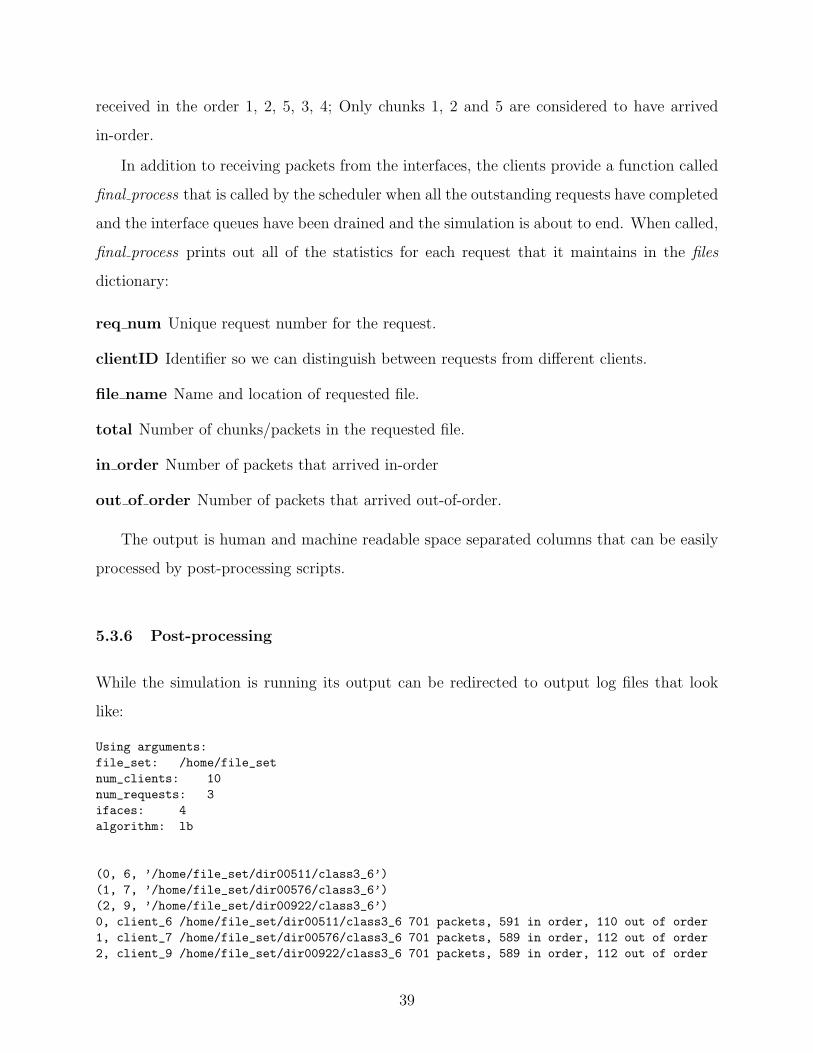
req num Unique request number for the request.

clientID Identifier so we can distinguish between requests from different clients.

file name Name and location of requested file.

total Number of chunks/packets in the requested file.

in order Number of packets that arrived in-order

out of order Number of packets that arrived out-of-order.

The output is human and machine readable space separated columns that can be easily

processed by post-processing scripts.

5.3.6 Post-processing

While the simulation is running its output can be redirected to output log files that look

like:

Using arguments:

file_set: /home/file_set

num_clients: 10

num_requests: 3

ifaces: 4

algorithm: lb

(0, 6, ’/home/file_set/dir00511/class3_6’)



0, client_6 /home/file_set/dir00511/class3_6 701 packets, 591 in order, 110 out of order



39

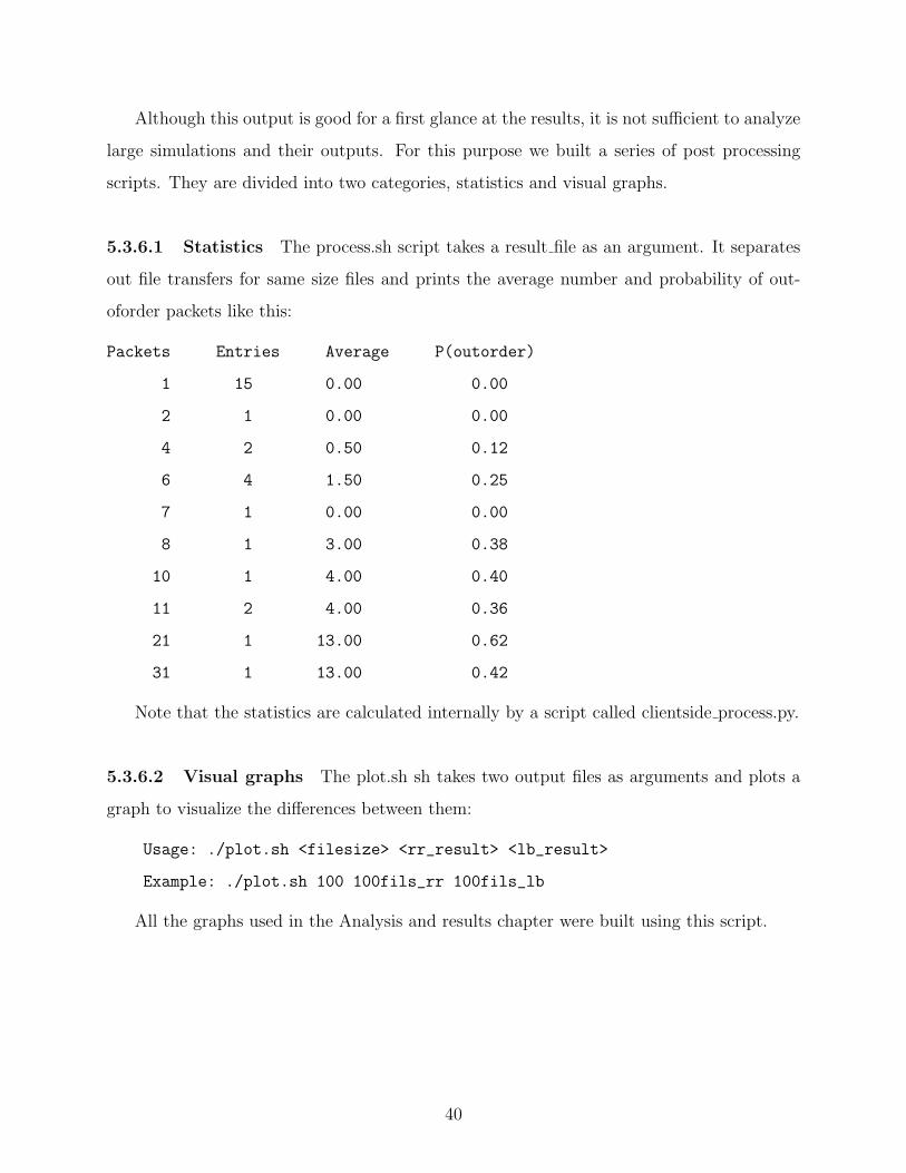
Although this output is good for a first glance at the results, it is not sufficient to analyze

large simulations and their outputs. For this purpose we built a series of post processing

scripts. They are divided into two categories, statistics and visual graphs.

5.3.6.1 Statistics The process.sh script takes a result file as an argument. It separates

out file transfers for same size files and prints the average number and probability of out-

oforder packets like this:

Packets Entries Average P(outorder)

1 15 0.00 0.00

2 1 0.00 0.00

4 2 0.50 0.12

6 4 1.50 0.25

7 1 0.00 0.00

8 1 3.00 0.38

10 1 4.00 0.40

11 2 4.00 0.36

21 1 13.00 0.62

31 1 13.00 0.42

Note that the statistics are calculated internally by a script called clientside process.py.

5.3.6.2 Visual graphs The plot.sh sh takes two output files as arguments and plots a

graph to visualize the differences between them:

Usage: ./plot.sh <filesize> <rr_result> <lb_result>

Example: ./plot.sh 100 100fils_rr 100fils_lb

All the graphs used in the Analysis and results chapter were built using this script.

40

6.0 ANALYSIS AND RESULTS

With the help of the BondingSimulator discussed in chapter 5 we implemented and tested

our hypothesis that load-based scheduling should be effective in significantly cutting down

the number of packets received out-of-order with round-robin scheduling. In the rest of this

chapter we describe our experiments to analyze the performance between the two algorithms

and present the results.

6.1 ANALYSIS OF SCHEDULING ALGORITHMS

We start our analysis by first understanding the two scheduling algorithms we implemented

and the expected outcomes of the experiments we did with the BondingSimulator.

1 5 2117139IF 0

2 6 181410X 22IF 1

IF 2

4 8 201612X 24IF 3

3 7 23191511

Figure 6: Example of Round Robin Scheduling

41

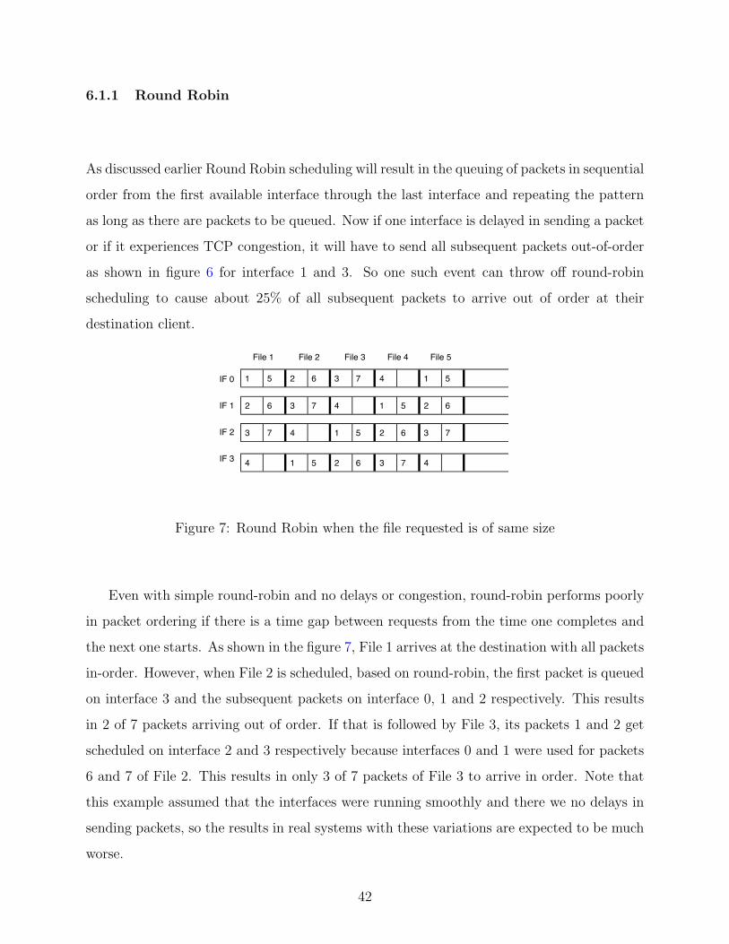
6.1.1 Round Robin

As discussed earlier Round Robin scheduling will result in the queuing of packets in sequential

order from the first available interface through the last interface and repeating the pattern

as long as there are packets to be queued. Now if one interface is delayed in sending a packet

or if it experiences TCP congestion, it will have to send all subsequent packets out-of-order

as shown in figure 6 for interface 1 and 3. So one such event can throw off round-robin

scheduling to cause about 25% of all subsequent packets to arrive out of order at their

destination client.

IF 0

IF 1

IF 2

IF 3

2 6 3 7 4 1 5 2 6

1 5 2 6 3 7 4 1 5

3 7 4 1 5 2 6 3 7

4 1 5 2 6 3 7 4

File 1 File 2 File 3 File 4 File 5

Figure 7: Round Robin when the file requested is of same size

Even with simple round-robin and no delays or congestion, round-robin performs poorly

in packet ordering if there is a time gap between requests from the time one completes and

the next one starts. As shown in the figure 7, File 1 arrives at the destination with all packets

in-order. However, when File 2 is scheduled, based on round-robin, the first packet is queued

on interface 3 and the subsequent packets on interface 0, 1 and 2 respectively. This results

in 2 of 7 packets arriving out of order. If that is followed by File 3, its packets 1 and 2 get

scheduled on interface 2 and 3 respectively because interfaces 0 and 1 were used for packets

6 and 7 of File 2. This results in only 3 of 7 packets of File 3 to arrive in order. Note that

this example assumed that the interfaces were running smoothly and there we no delays in

sending packets, so the results in real systems with these variations are expected to be much

worse.

42

6.1.2 Load Based

We propose that load-based scheduling of packets would be a significant improvement over

round-robin. In case of Load based, rather than putting packets in a round-robin manner, we

look at the current queue size of each interface and then send the next packet to the interface

which has least number of outstanding packets in its queue. If more than one interface have

the least number of packets, we choose the lowest of them. This results in round-robin

scheduling between the interfaces with the same lowest queue size, thereby ensuring that our

algorithm will perform at least as well as round-robin in all cases.

1 5 1915139 23IF 0

2 6 201610X 24IF 1

IF 2

4 8 221812XIF 3

3 7 21171411

Figure 8: Example of Load based scheduling

As shown in figure 8, initially we start off by queuing packets 1 through 12 sequentially

on the four interfaces. However, at this point interfaces 1 and 3 experience a delay and

packets 10 and 12 don’t get sent on time. The load-based scheduling algorithm notices

this discrepancy and schedules packets 13 and 14 on interfaces 0 and 2 while skipping the

loaded interfaces 1 and 3 thus allowing those interfaces to catch up. This is followed by all

subsequent packets arriving in-order. So only 2 of 24 packets or about 8% of the packets

arrive out-of-order.

So, our analysis shows that load based scheduling should be significantly better than

round-robin in delivering packets in-order to the requesting clients. We then proceeded to

test this with the BondingSimulator.

43

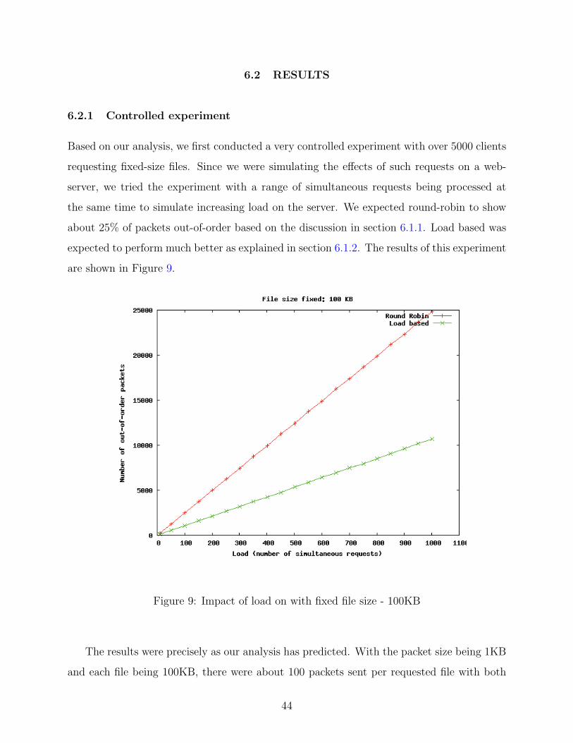
6.2 RESULTS

6.2.1 Controlled experiment

Based on our analysis, we first conducted a very controlled experiment with over 5000 clients

requesting fixed-size files. Since we were simulating the effects of such requests on a web-

server, we tried the experiment with a range of simultaneous requests being processed at

the same time to simulate increasing load on the server. We expected round-robin to show

about 25% of packets out-of-order based on the discussion in section 6.1.1. Load based was

expected to perform much better as explained in section 6.1.2. The results of this experiment

are shown in Figure 9.

Figure 9: Impact of load on with fixed file size - 100KB

The results were precisely as our analysis has predicted. With the packet size being 1KB

and each file being 100KB, there were about 100 packets sent per requested file with both

44

round-robin and load-based algorithms. As figure 9 shows, we expected about 25 out-of-order

packets per request1 with round-robin. With 100 simultaneous requests, we expected about

25 * 100 = 2500 out-of-order packets evidenced by the second data point for the red plot.

The corresponding green data point for load-based shows that the algorithm was able to cut

down the number of out-of-order packets by about 50% in our experiments. This accurate

result that matched our expectations helped us gain confidence that our implementation of

the two algorithms was performing as expected under controlled conditions and could serve

as the basis for more sophisticated realistic scenarios.

6.2.2 Varying load on server

Figure 10: Impact of load on out-of-order with varying file size

The second experiment we conducted was to include files of varying file sizes in the

1100KB file = 100 packets, 1KB each

45

requests. This makes the simulation more realistic as compared to a web-server serving

requests for a number of files with a wide range of file sizes. In our experiment we varied

the file size from 1KB to 900KB and analyzed the results of load on out-of-order packets for

the two algorithms.

As shown in figure 10, we got results quite similar to our controlled experiment. There

is a slight variation in the results because the requested files vary in size and hence, end

at different times during the simulation as against the uniform distribution of file endings

in the controlled experiment. The varying file sizes cause these deviations because when a

small requested file ends, the interface is freed up for the remaining transfers to use. These

results demonstrate that load-based scheduling consistently performs better than round-

robin with about 50% less out-of-order packets, even with increasing load and varying file

sizes. However, the number of order packets may vary if the experimental conditions are

changed.

6.2.3 Probability

As shown in figure 11 we also calculated the probability of getting out-of-order packets for

different file sizes and noticed that no matter what is the file size, the Probability remains

constant for both Round robin and Load based. In our previous experimets one interface

was running slower than other, so we had 25% of packets out of order in case of Round robin

and about 10% out-of-order in Load based. However in our experimets for Probability, we

had two interfaces running slower and thus the number of out of order packets increased.

The number of out-of-order in case of Round robin as we can see in probability graph is

about 50% and in case of Load based it is about 25%.

6.2.4 Other observations

While running our experiments to simulate a slower network interface card, we noticed that

round-robin simulations were taking much longer to complete as compared to load-based.

The reason for this was that since round-robin blindly queues an equal number of packets on

each network interface card, if one card is running slower than others, it would have to catch

46

Figure 11: Probability of getting out-of-order Packets

47

up near the end of the simulation. The end result of this effect was that the faster network

interface cards would complete processing their queues and then sit idle while the slower

interface card(s) completed their work. This can have a significant impact on production

systems. If one interface is running slower on a system running round-robin, there is a

significant amount of risk of queue overflow on that interface when the system experiences

a high load. Our proposed load-based algorithm is not affected with this adverse effect

because it distributes packets based on the interface queue size thereby ensuring that slower

interfaces do not get overloaded in such situations.

Another important observation during these experiments was that the number of out-

of-order packets with load-based scheduling was directly and linearly proportional to the

number of delays or congestion events at the interfaces. Whereas, with round-robin, one

single event can cause all of the packets queued on that interface to arrive out-of-order. This

further strengthens our claim that load-based scheduling not only reduces the number of

out-of-order packets but also keeps the number of out-of-order packets predictable under

varying load and network conditions.

48

7.0 CONCLUSION

Our work presented load-based scheduling as a significant improvement over round-robin

scheduling for NIC bonding to reduce the number of packets that are delivered out-of-order

and therby increasing the performance of NIC bonding. Our proposed solution cuts down the

number of out-of-order packets by more than 50% and provides predictability of out-of-order

packets if the number of network events such as delays and congestion are known. We also

demonstrated that load-based scheduling distributes packets such that no single interface

is slowing down all connections because it is running slower than the other interfaces on

the system. In addition, we also developed a NIC bonding simulation framework to allow

for future development and analysis of various aspects of NIC bonding including scheduling

algorithms.

7.1 FUTURE WORK

As shown by our work, even though NIC bonding has been implemented and used in net-

working infrastructure for quite some time, there are significant research and development

opportunities in this area. To further the ideas presented in our work, we would like to

collect real-time traces from a production web server in future. These traces can then be

used to control the timing of various components of our simulation and allow for realistic

system analysis.

Another step would be to implement the proposed load-based scheduling algorithm as a

bonding mode for the Linux kernel and evaluate it on a production system. This would be

implemented as a new bonding mode in the bonding driver. We would have to implement

49

an interrupt for the interfaces so they can report their current queue size without the driver

having to calculate it for every packet.

We can also vary the packet size to accurately simulate a realistic network with different

arrival rates for different sized packets. This may cause more deviation in the output but

the slopes should still remain the same.

Another interesting research direction would be to measure the number of out-of-order

packets on live networks using round-robin bonding mode. This would help us understand

how significantly the out-of-order packets affect such networks and evaluate the advantage

of our work in real deployments.

50

BIBLIOGRAPHY

[1] Ahmed Abd El Al, Tarek Saadawi, and Myung Lee. Ls-sctp: a bandwidth aggregationtechnique for stream control transmission protocol. Computer Communications, 27(10),2004.

[2] Josep M. Blanquer. Fair queuing for aggregated multiple links. In in Proc. Sigcomm2001, pages 189–197, 2001.

[3] Peter Brucker. Scheduling Algorithms. Springer Berlin Heidelberg, 2009.

[4] Alan Burns. Preemptive priority based scheduling: An appropriate engineering ap-proach. In PRINCIPLES OF REAL-TIME SYSTEMS, pages 225–248. Prentice Hall,1994.

[5] Anna Charny and JY Boudec. Delay bounds in a network with aggregate scheduling.Quality of Future Internet Services, 2000.

[6] cnet. Amazon downtime. http://news.cnet.com/8301-107843-9962010-7.html,2009.

[7] LXR community. Linux/driver/net/bonding. http://lxr.linux.no/linux+v2.6.29/drivers/net/bonding/, 2009.

[8] Dell. Link aggregation on the dell poweredge 1855 server ethernet switch. http://support.dell.com/support/edocs/network/LAG1855/LAGConsiderationv0.5.pdf,2005.

[9] Sally Floyd. Link-sharing and resource management models for packet networks.IEEE/ACM Transactions on Networking, 3:365–386, 1993.

[10] Linux foundation. Nic bonding. http://www.linuxfoundation.org/collaborate/workgroups/networking/bonding, 2009.

[11] Jason Gabler. Better bonded ethernet load balancing. http://www.osti.gov/energycitations/product.biblio.jsp?osti id=883778, 2006.

51

http://lxr.linux.no/linux+v2.6.29/drivers/net/bonding/

http://lxr.linux.no/linux+v2.6.29/drivers/net/bonding/

http://support.dell.com/support/edocs/network/LAG1855/LAGConsiderationv0.5.pdf

http://support.dell.com/support/edocs/network/LAG1855/LAGConsiderationv0.5.pdf

http://www.linuxfoundation.org/collaborate/workgroups/networking/bonding

http://www.linuxfoundation.org/collaborate/workgroups/networking/bonding

http://www.osti.gov/energycitations/product.biblio.jsp?osti_id=883778

http://www.osti.gov/energycitations/product.biblio.jsp?osti_id=883778

[12] E. L. Hahne and R. G. Gallager. Round robin scheduling for fair flow control in datacommunication networks. IEEE International Conference on Communications, June1986.

[13] Mor Harchol-balter, Bianca Schroeder, Mukesh Agrawal, and Nikhil Bansal. Size-basedscheduling to improve web performance. ACM Transactions on Computer Systems,21:207–233, 2003.

[14] E. S. H. Hou, N. Ansari, and H. Ren. A genetic algorithm for multiprocessor scheduling.IEEE Transactions on Parallel and Distributed Systems, 5(2):113–120, 1994.

[15] Cisco Systems Inc. Internetworking Technologies Handbook. Cisco Press, 2003.

[16] C. L. Liu and James W. Layland. Scheduling algorithms for multiprogramming in ahard-real-time environment. ACM, 20(1), 1973.

[17] J. Luo, L. Xu, and J. S. Plank. An efficient XOR-Scheduling algorithm for erasurecodes encoding. In DSN-2009: The International Conference on Dependable Systemsand Networks, Lisbon, Portugal, June 2009. IEEE.

[18] BSD System Manager’s maual. ifconfig. http://developer.apple.com/mac/library/documentation/Darwin/Reference/ManPages/man8/ifconfig.8.html, 2004.

[19] Andrea Schaerf, Yoav Shoham, and Moshe Tennenholtz. Adaptive load balancing: Astudy in multi-agent learning. Journal of Artificial Intelligence Research, 2:475–500,1995.

[20] Howard Frazier Broadcom Schelto, Van Doorn Intel, Robert Hays Intel, Shimon MullerSun Microsystems, Bruce Tolley Solarflare Communications, Paul Kolesar CommScope,Geoff Thompson Nortel, and Brad Turner. Ieee 802.3ad link aggregation (lag) what itis and what it is not. Juniper Networks, 2007.

[21] M. Shreedhar, Microsoft Corp., WA Seattle, and George Varghese Washington Univ. Ef-ficient fair queueing using deficit round-robin. IEEE/ACM Transactions on Networking(TON), 4(3), June 1996.

[22] Sander van Vugt. Pro Ubuntu Server Administration. Apress; 1 edition, 2008.

[23] Chih wen Hsueh, Hsin hung Lin, and Guo-Chiuan Huang. Channel bonding in linuxethernet environment using regular switching hub. Journal of Systemics, Cyberneticsand Informatics, 2(3), 2004.

[24] Jingnan Yao, Jiani Guo, and Laxmi Narayan Bhuyan. Ordered round-robin: An efficientsequence preserving packet scheduler. IEEE Transactions on Computers, 57(12), 2008.

52

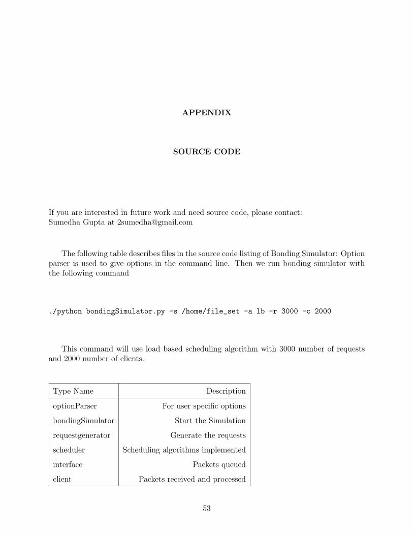
http://developer.apple.com/mac/library/documentation/Darwin/Reference/ManPages/man8/ifconfig.8.html

http://developer.apple.com/mac/library/documentation/Darwin/Reference/ManPages/man8/ifconfig.8.html

APPENDIX

SOURCE CODE

If you are interested in future work and need source code, please contact:Sumedha Gupta at [email protected]

The following table describes files in the source code listing of Bonding Simulator: Optionparser is used to give options in the command line. Then we run bonding simulator withthe following command

./python bondingSimulator.py -s /home/file_set -a lb -r 3000 -c 2000

This command will use load based scheduling algorithm with 3000 number of requestsand 2000 number of clients.

Type Name Description

optionParser For user specific options

bondingSimulator Start the Simulation

requestgenerator Generate the requests

scheduler Scheduling algorithms implemented

interface Packets queued

client Packets received and processed

53

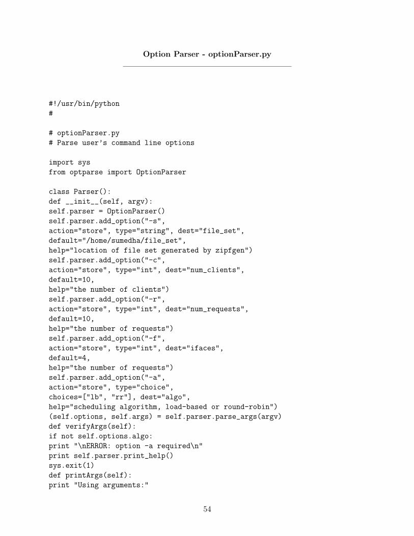
Option Parser - optionParser.py

#!/usr/bin/python#

# optionParser.py# Parse user’s command line options

import sysfrom optparse import OptionParser

class Parser():def __init__(self, argv):self.parser = OptionParser()self.parser.add_option("-s",action="store", type="string", dest="file_set",default="/home/sumedha/file_set",help="location of file set generated by zipfgen")self.parser.add_option("-c",action="store", type="int", dest="num_clients",default=10,help="the number of clients")self.parser.add_option("-r",action="store", type="int", dest="num_requests",default=10,help="the number of requests")self.parser.add_option("-f",action="store", type="int", dest="ifaces",default=4,help="the number of requests")self.parser.add_option("-a",action="store", type="choice",choices=["lb", "rr"], dest="algo",help="scheduling algorithm, load-based or round-robin")(self.options, self.args) = self.parser.parse_args(argv)def verifyArgs(self):if not self.options.algo:print "\nERROR: option -a required\n"print self.parser.print_help()sys.exit(1)def printArgs(self):print "Using arguments:"

54

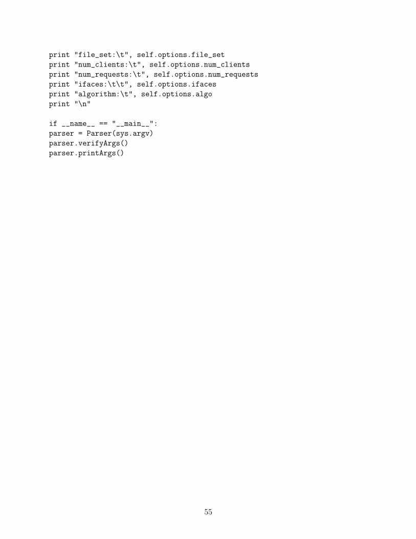
print "file_set:\t", self.options.file_setprint "num_clients:\t", self.options.num_clientsprint "num_requests:\t", self.options.num_requestsprint "ifaces:\t\t", self.options.ifacesprint "algorithm:\t", self.options.algoprint "\n"

if __name__ == "__main__":parser = Parser(sys.argv)parser.verifyArgs()parser.printArgs()

55

Bonding simulator - bondingSimulator.py

#!/usr/bin/python#

from twisted.internet import reactor

import osimport sysfrom random import randint

from client import clientfrom scheduler import schedulefrom interface import ifacefrom requestGenerator import requestfrom optionParser import Parser

def bondingSimulator(file_set, num_clients, ifaces, requests, algo):client_list = []iface_list = []

# Create a request generatorrequestor = request(file_set, num_clients, requests)# Start generating requests and queuing themrequestor.generate()

# Create the clientsfor i in range(0, num_clients):client_obj = client(i)client_list.append(client_obj)

# Create the interfacesfor i in range(0, ifaces):iface_obj = iface(i, client_list)iface_list.append(iface_obj)iface_obj.process_pending()

# Create the scheduler that will process the requests from requestorscheduler = schedule(algo, requestor.request_queue, iface_list, client_list)

# Start processing requestsscheduler.process()

56

# Start the simulationreactor.run()

if __name__ == "__main__":

parser = Parser(sys.argv)parser.verifyArgs()parser.printArgs()

file_set = parser.options.file_setnum_clients = parser.options.num_clientsnum_requests = parser.options.num_requestsifaces = 4algo = parser.options.algobondingSimulator(file_set, num_clients, ifaces, num_requests, algo)

57

Request generator - requestGenerator.py

#!/usr/bin/python#


import osimport sysimport globfrom random import randint

class request():def __init__(self, file_set, num_clients, requests):self.request_queue = []self.file_set = file_setself.num_clients = num_clientsself.num_requests = requestsself.requested = 0

def random_file_name(self):# Return a random file name

num_dirs = len(os.listdir(self.file_set))num_dirs = num_dirs - 1# We pick a file from directory above 00009 for smaller files#file_name = "%s/dir%05d/class3_0" % \# (self.file_set, randint(10,num_dirs))file_name = (glob.glob("%s/dir%05d/class3_*" % \(self.file_set, randint(10,num_dirs))))[0]#file_name = "%s/dir%05d/class%d_%d" % \# (self.file_set, randint(10,num_dirs), \# randint(0,3), randint(0,8))return file_name

def random_client_name(self):# Return a random client namereturn randint(0, self.num_clients-1)

# Random request is puting data in a request generator with# random_client_name() and random_file_name() in it.

def random_request(self):client = self.random_client_name()

58

file_name = self.random_file_name()# Each request contains req_num, client_id and file_namereturn (self.requested, client, file_name)

# Main is calling generate(), generate is calling random request()# with callLater

def generate(self):for i in range(1,5000):if(self.requested >= self.num_requests):returnrequest = self.random_request()print requestself.request_queue.append(request)self.requested = self.requested + 1reactor.callLater(5, self.generate)#reactor.callLater(randint(1,5), self.generate)

59

Scheduler - scheduler.py

#!/usr/bin/python#


import osimport sys

# Schedule will get the pointer of request_queue from request.class schedule():def __init__(self, algo, queue, iface_list, client_list, chunk_size=1024):self.algo = algoself.iface_list = iface_listself.client_list = client_listself.ifaces = len(iface_list)self.next_iface=0self.queue = queueself.next_req = 0self.chunk_size = chunk_sizeself.fd_dict = {}self.file_chunk = {}self.watchdog = 200

def queue_packet_to_iface_rr(self, request):# Extract clientID and filename from requestreq_num, client, filename = request

# Find the file descriptor for the requested filefd = self.fd_dict[req_num]

# Read a chunk of data from the filebuf = fd.read(self.chunk_size)

# queue chunk to the next interface#print "queue: IF %d: " % self.next_iface,#print "Client_%d, %s, chunk: %d" % \# (client, filename, self.file_chunk[req_num])self.iface_list[self.next_iface].queue( \req_num, client, filename, self.file_chunk[req_num])

60

# Increment the file_chunk number for this fileself.file_chunk[req_num] = self.file_chunk[req_num] + 1

# Pick the next interface that we’ll queue the next packet toself.next_iface = (self.next_iface+1) % self.ifaces

# If this was the last chunk in the fileif (len(buf) < self.chunk_size):# Remove request from queueself.queue.remove(request)# Close file and forget its descriptorself.fd_dict[req_num].close()del self.fd_dict[req_num]# Remove file_chunk trackingdel self.file_chunk[req_num]

def queue_packet_to_iface_lb(self, request):# Extract clientID and filename from requestreq_num, client, filename = request

# Find the file descriptor for the requested filefd = self.fd_dict[req_num]

# Read a chunk of data from the filebuf = fd.read(self.chunk_size)

# queue chunk to the interface with smallest queuelowest_q = 100000000for iface in self.iface_list:q_size = iface.q_size()#print "Interface_%d, %d:" %(iface.iface_num, q_size)if lowest_q > q_size:lowest_q = q_sizelowest_iface = iface#print "queue: IF %d: " % self.next_iface,#print "Client_%d, %s, chunk: %d" % \# (client, filename, self.file_chunk[req_num])lowest_iface.queue( \req_num, client, filename, self.file_chunk[req_num])

# Increment the file_chunk number for this fileself.file_chunk[req_num] = self.file_chunk[req_num] + 1

# Pick the next interface that we’ll queue the next packet to#self.next_iface = (self.next_iface+1) % self.ifaces

61

# If this was the last chunk in the fileif (len(buf) < self.chunk_size):# Remove request from queueself.queue.remove(request)# Close file and forget its descriptorself.fd_dict[req_num].close()del self.fd_dict[req_num]# Remove file_chunk trackingdel self.file_chunk[req_num]

def process(self):

# Open all requested files and save the descriptors in fd_dictfor request in self.queue:# Open the requested filereq_num, client, filename = requestif req_num not in self.fd_dict:fd = open(filename, ’r’)self.fd_dict[req_num] = fdself.file_chunk[req_num] = 0

# Decrement the watchdog if queue is emptyif len(self.queue) == 0:self.watchdog = self.watchdog - 1

# Read each entry in request_queue#for request in self.queue[:]:for req in range (0,4):if len(self.queue) <= 0:breakrequest = self.queue[self.next_req]if self.algo == "rr":self.queue_packet_to_iface_rr(request)if self.algo == "lb":self.queue_packet_to_iface_lb(request)if len(self.queue)<= 0:breakself.next_req = (self.next_req + 1) % len(self.queue)self.watchdog = 200

# If no more requests are coming, we stop the simulationif self.watchdog <= 0:allzero = Truefor iface in self.iface_list:

62

q_size = iface.q_size()if q_size != 0:allzero = False

if allzero:for client in self.client_list:client.final_process()reactor.stop()

# Done queuing all outstanding requests to interfaces# Check for new requests after some timereactor.callLater(0.020, self.process)

63

Interface - interface.py

#!/usr/bin/python#

from twisted.internet import reactorfrom random import randint

import osimport sysimport time

class iface():def __init__(self, num, clientList):self.pending = []self.iface_num = numself.clientList = clientList

def queue(self, req_num, client, file_name, chunk):self.pending.append((req_num, client, file_name, chunk))

def q_size(self):return len(self.pending)

def process_pending(self):#print "%d: pending: %d" % (self.iface_num, len(self.pending))if(len(self.pending) > 0):packet = self.pending.pop(0)(req_num, client, file_name, chunk) = packet#print "IF %d: send: client_%d file: %s chunk: %d" % \# (self.iface_num, client, file_name, chunk)self.clientList[client].send(req_num, file_name, chunk)

#nextCall = randint(200, 201)/10000.0if (self.iface_num == 0):

nextCall = .020#nextCall = randint(20,22)/1000.0

if (self.iface_num == 1):nextCall = .082#nextCall = randint(22,24)/1000.0

if (self.iface_num == 2):nextCall = .020

64

#nextCall = randint(20,23)/1000.0if (self.iface_num == 3):

nextCall = .020#nextCall = randint(20,22)/1000.0

reactor.callLater(nextCall, self.process_pending)

65

Client - client.py

#!/usr/bin/python#


import osimport sys#import time

class client():def __init__(self, id):self.clientID = idself.files = {}

# Receive packets from interfacesdef send(self, req_num, file_name, chunk):#print self.clientID#receiving_time = time.time()#print "Receiving time = %f " % receiving_time#print "client:%d got %s, chunk: %d" % \# (self.clientID, file_name, chunk)

# If this is not a file we know of, add it to our files listif req_num not in self.files:self.files[req_num] = (file_name, chunk, 1, 1)return

# Get the total and in_order packets for the file_name(file_name, last, total, in_order) = self.files[req_num]total = total + 1

# If the new chunk number is higher, this packet is in-orderif chunk > last:in_order = in_order + 1last = chunk

# Store the new values back in the files listself.files[req_num] = (file_name, last, total, in_order)

def final_process(self):

66

for req_num in self.files.keys():(file_name, last, total, in_order) = self.files[req_num]out_of_order = total - in_orderprint "%d, client_%d %s %d packets, %d in order, %d out of order" % \(req_num, self.clientID, file_name, total,in_order,out_of_order)

def process_pending(self):reactor.callLater(0.10, self.process_pending)

67

impact of load-based nic-bonding scheduling on out...

Documents