Physica A 392 (2013) 4435–4449

Contents lists available at SciVerse ScienceDirect

Physica A

journal homepage: www.elsevier.com/locate/physa

Impact of monetary policy changes on the Chinese monetaryand stock marketsYong Tang a,b,∗, Yong Luo a, Jie Xiong c, Fei Zhao a, Yi-Cheng Zhang b

a School of Management and Economics, University of Electronic Science and Technology of China, Chengdu Sichuan, 610054, Chinab Department of Physics, University of Fribourg, Chemin du Musée 3, CH-1700 Fribourg, Switzerlandc Department of Information Systems and Quantitative Analysis, College of Information Systems and Technology, University ofNebraska at Omaha, Omaha, NE 68182, USA

h i g h l i g h t s

• The impact of Chinese monetary policy change surprises on the SHIBOR monetary market and stock market is studied.• Sign effect is observed on announcing and effective dates.• Relative larger fluctuation is observed before event dates.• Lowering policy drive stock market climb with a delay of 2 days.• In the bear market, a lowering policy change brings larger volatility in stock market.

a r t i c l e i n f o

Article history:Received 4 November 2012Received in revised form 30 April 2013Available online 24 May 2013

Keywords:EconophysicsMonetary policySHIBORStock market

a b s t r a c t

The impact of monetary policy changes on themonetarymarket and stockmarket in Chinais investigated in this study. The changes of two major monetary policies, the interestrate and required reserve ratio, are analyzed in a study period covering seven years onthe interbank monetary market and Shanghai stock market. We find that the monetarymarket is related to the macro economy trend and we also find that the monetary changesurprises both of lowering and raising bring significant impacts to the two markets andthe two markets respond to the changes differently. The results suggest that the impactof fluctuations is much larger for raising policy changes than lowering changes in themonetary market on policy announcing and effective dates. This is consistent with the‘‘sign effect’’, i.e. bad news brings a greater impact than good news. By studying the eventwindow of each policy change, we also find that the ‘‘sign effect’’ still exists before andafter each change in themonetarymarket. A relatively larger fluctuation is observed beforethe event date, which indicates that the monetary market might have a certain ability topredict a potential monetary change, while it is kept secret by the central bank beforeofficial announcement. In the stock market, we investigate how the returns and spreads ofthe Shanghai stock market index respond to the monetary changes. Evidences suggest thestockmarket is influenced but in a differentway than themonetarymarket. The climbing ofreturns after the event dates for the lowering policy agrees with the theory that loweringchanges can provide a monetary supply to boost the market and drive the stock returnshigher but with a delay of 2 to 3 trading days on average. While in the bear market, theloweringpolicy brings larger volatility to themarket on average than the raising ones. Theseempirical findings are useful for policymakers to understand howmonetary policy changesimpact themonetary and stockmarkets especially in an emergingmarket like Chinawhere

∗ Corresponding author at: Department of Physics, University of Fribourg, Chemin du Musée 3, CH-1700, Fribourg, Switzerland. Tel.: +86 13880206370.E-mail address: yong.tang@unifr.ch (Y. Tang).

0378-4371/$ – see front matter© 2013 Elsevier B.V. All rights reserved.http://dx.doi.org/10.1016/j.physa.2013.05.023

4436 Y. Tang et al. / Physica A 392 (2013) 4435–4449

the economy is booming and the policy changes impact the markets as surprises by thecentral bankwithout a pre-decided schedule. This is totally different from previous studieson FED, which follows pre-decided schedules for monetary policy changes.

© 2013 Elsevier B.V. All rights reserved.

1. Introduction

Monetary policy changesmade by the central bank of each country can bring a great influence to the financialmarkets [1].A central bank can lower or raise benchmark rates to adjust the economy, which is similar to the interest rate. Severalresearchers [2–7] study how the Federal Reserve Board(FED), the central bank of the United States influences the marketsboth from the traditional finance research perspective [2,8–11] and statistical physics [12,13]. Some studies report stockmarkets respond differently to different policy actions and types [2,5]. For other countries and regions like South EastAsia [14], the link between monetary policy and asset prices is also investigated. In study [15], the results suggest there isasymmetrical volatility before and after a Federal Open Market Committee (FOMC) meeting event in the Irish stock market.Similar research is conducted in the markets from Germany and the UK, where asset prices are negatively influenced bythe UK monetary policy changes [16]. In the Euro Area, studies [17–20] focus on how the monetary policy changes madeby the European Central Bank (ECB) can influence the markets. Expansionary monetary policy can lead to higher marketliquidity in German, French and Italian markets [18], the ECB makes a clear impact on volatilities of the European indexreturn [19]. The monetary policy changes are also studied from 13 countries in the Organization for Economic Co-operationandDevelopment (OECD) [21] andCanada [22]. Awider collection of 16 countries are investigated inRef. [23] and the authorsfind monetary policy changes influence the stock market returns on a monthly and quarterly basis. However, there is still alack of study on how the market responds to the monetary changes in emerging markets like China, since the mechanismsof monetary policy changes adapted by other central banks might be different between developed countries and emergingmarkets like China.While some studies only focus on how the stockmarket responds [24], it is important to investigate howthe monetary market responds to the monetary policy changes in China.

In this paper, we conduct research on the impact of the monetary policy changes made by the central People’s Bank ofChina (PBC) to the monetary market and the stock market. Results of analysis suggest that the Shanghai Interbank OfferedRate (SHIBOR) monetary market and Shanghai stock market respond differently to the changes of interest rate (R) andrequired reserve ratio (RRR). In a bear market, lowering R or RRR can bring a larger fluctuation into the stock market and asmaller fluctuation into themonetarymarket. There is a significant ‘‘sign effect’’ [12,25] that raising RRR or R can bring largerfluctuations to the SHIBORmarket, while raising policieswill impact themonetarymarketsmore. For the stockmarket, thereis an approximately two-day-delay for lowering policies to take effect, to drive the stock market index higher, which alsoagrees with the fact that lowering policies can provide a stronger money supply into the market and boost the market. Forthe SHIBOR market, the average fluctuations reach peaks at 1 or 2 days before the policy changes announcement dates andeffective dates. This indicates the SHIBOR market has a certain predictability for monetary change surprises which the PBCkeeps secret and releases as surprises without any schedules. All the 34 RRR changes and 16 R changes between 2006-10-08and 2012-05-11, covering1401 trading days are studied in this research.

This paper is organized into four sections as follows. In Section 2, the Chinese monetary policy tools of RRR and R, theChinese interbank monetary market index SHIBOR and the Shanghai stock market are introduced. In Section 3, the researchmethod and data collection results with analysis are presented. The conclusions, discussions, contributions, and limitationsare provided in Section 4.

2. Chinese monetary policy, SHIBOR and Shanghai stock market

After nearly thirty years of miraculous economic development since the 1980s with a stunning annual Gross DomesticProduct (GDP) growth of over 8%, China has built an expanding economy that has overtaken Japan as the second-biggestonly after the US and is expected to replace the US as the world’s largest economy in the near future. While enjoying ahuge economic boom, China is also suffering from serious problems of rising salary, energy and raw material costs alongwith the huge pressure to raise the Renminbi Yuan (RMB) currency exchange rate which erodes China’s exports, a rapidlyclimbing Consumer Price Index (CPI), and speculating demand for property. It is a great challenge and also a top priorityfor the Chinese government to maintain an economic growth rate at the same high level while taming persistent inflation.China sticks to a so-called appropriate loose monetary policy in order to achieve healthy economic development.

The People’s Bank of China (PBC), the central bank of China, plays a similar role of monetary policy maker as the FEDreserve in the US to maintain the stability of the value of the currency and thereby promote economic growth. In PBC’smonetary policy toolbox, major instruments are reserve requirement ratio (RRR), central bank base interest rate (R), redis-counting, central bank lending, and open market operation [26]. Among them, RRR and R have a significant influence overthe market and draw great attention from the public. What makes it more interesting is that the PBC’s monetary committeeannounces all of the changes of both rates as sudden surprises without schedules. This is quite different from the way FEDreserve makes rate change announcements, which will mostly follow a pre-determined schedule of Federal Open Market

Y. Tang et al. / Physica A 392 (2013) 4435–4449 4437

Committee (FOMC) meetings. Once PBC announces the changes of RRR or R, the money market and stock market will beimpacted and be forced to respond to the new policy by absorbing the information in the markets. Since the changes comeas surprises, themarket is not likely to predict exactly the announcing dates but themarket activities will reflect themarketexpectation of a coming monetary policy change.

RRR is a PBC regulation which demands the minimum reserves ratio for each commercial bank deposit made with PBCto its total customer deposits. Because of the exponential effect, which means loaned money can be re-loaned to generatemore money in the market, PBC uses RRR as a major inflation-fighting monetary policy tool by normally raising the RRR tolower the exponential effect in order to reduce the money supply to the market andmaintain the money purchasing power.RRR changes are announced by PBC suddenly but the targeted ratio is set to be effective with a time lag of more than a weeknormally. Due to the 2008 financial crisis, the PBC adapted a new RRR policy demanding a different RRR for large financialinstitutes and medium–small financial institutes respectively. While the large financial institutes like commercial banksand institutional investors are the most influential major players in the market, we will focus on the RRR for large financialinstitutes in this research.

PBC’s interest rate (R) is also another tool to battle against the high inflation and bubbles in property and other markets.The benchmark one-year (1Y) deposit rate and lending rate are raised as surprises in order to lower the market investmentsand also ease the pressure of the appreciation of RMB by lockingmoremoney in banks and raising the cost ofmoney lending.PBC normally sets the effective day on the same announcing day or the following day. The direct result of a climbing Rwill push commercial banks to raise the interbank interest rates, which leads to a higher lending cost between financialinstitutions and lower speculation in the market. For each R change, PBC sets two benchmark one-year bank rates to lendand deposit rates respectively. Generally speaking, the lending rate is higher than the deposit rate, but these two rates sharesimilar movements. Since we investigate the ask prices between banks which aremore closely relatedwith the lending rate,so in this study we choose to use the lending interest rate.

The Shanghai Interbank Offered Rate (SHIBOR) is the Chinese version of the London Interbank Offered Rate (LIBOR) andFederal Funds Interest Rates. By arithmetically averaging all the interbank RMB bid–ask rates offered by a group of 16quotation banks, which are major active players in the RMB money market with high credit ratings, the National InterbankFunding Center (NIFC) in Shanghai announces the daily SHIBOR rate of eight maturities from overnight, to one week, toone year. Among them the overnight is the most used daily rate by institutes in pricing financial products [27]. After theintroduction of SHIBOR in 2006, it has become the de facto interest rate market benchmark. Since SHIBOR is a result of openmarket trading games between commercial banks reflecting the money supply–demand situation in the market, SHIBORhas become a market index to measure the market liquidity and the market expectation to a potential monetary policychange. The two independently operating stockmarkets, Shanghai stockmarket (SHSM) and Shenzhen stockmarket (SZSM),together compose the Chinese stock market (CSM). The stock market is very sensitive to any monetary policy changes andthe market volatility is also a result of investor expectation. In this study, we use the daily index data of the Shanghai stockmarket where major industrial companies and financial companies are listed and focus on the dynamics of SHIBOR andSHSM responding to the monetary policy changes of RRR and R.

3. Data and results

In this part, we analyze the history of PBC’s changes of both RRR and R, all the SHIBOR daily prices and quotes, and thedaily index of SHSM for the 6-year-period from 2006/10/08 to 2012/05/11. The change dates are collected from the officialwebsite of the PBC and the SHIBOR data are collected from the SHIBOR data services [27]. Since SHIBOR was introduced in2006, we only use the RRR and R SHIBOR data, which are available from 2006 to 2012. To investigate the impact on the stockmarket, we use the Shanghai stock market index data during the same study period.

3.1. RRR and R

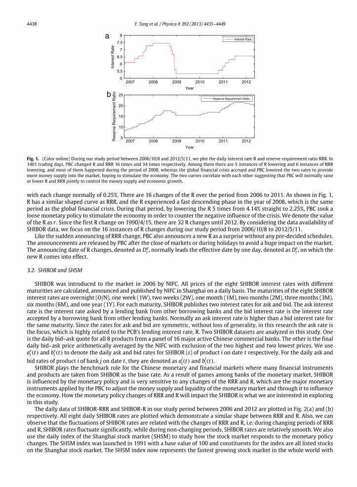
After the first time RRRwas introduced in 1984, there have been in total 46 changes of RRR until 2012.While the SHIBORwas first introduced in 2006, we only consider the RRR changes after the introduction of SHIBOR. During the study periodbetween2006/10/8 and2012/5/11, there have been34RRR changes. As shown in Fig. 1, theRRR is almost constantly climbingfrom 6% to a stunning high of 21% and normally with an increment of 0.5% for each time, except the period of the 2008–2009global financial crisis, during which RRR experienced a temporarily drop by 4% to counter the crisis. Before 2006, there wereonly 7 changes over 20 years, but after 2006, the PBC more and more frequently raised the RRR to control the economy, 33times in total, nearly 6 times per year. In the first five months of 2011, PBC even raised RRR 5 times monthly. In 2012, thereare 2 drops of RRR when the market needed stimulation and more money supply.

Normally, RRR changes are announced by PBC as surprises when markets are closed during evenings or during holidaysin order to minimize the impacts to markets. The dates on which RRR changes are announced are called RRR announcingdates or Da

rrr on which a new RRR and the effective date for the new RRR comes into effect are announced by the PBC. Theeffective dates on which the new RRR becomes effective, De

rrr , are normally about one week after the announcing dates, Darrr .

The value of the RRR is denoted as rrr .The interest rate R also has a great influence and impact on the markets. Before 2006, PBC did not frequently change the

R and maintained the R at a low level of 2.25%, but after 2006, PBC began to frequently change the R from 2.25% to 3.25%

4438 Y. Tang et al. / Physica A 392 (2013) 4435–4449

Fig. 1. (Color online) During our study period between 2006/10/8 and 2012/5/11, we plot the daily interest rate R and reserve requirement ratio RRR. In1401 trading days, PBC changed R and RRR 16 times and 34 times respectively. Among them there are 5 instances of R lowering and 6 instances of RRRlowering, and most of them happened during the period of 2008, whereas the global financial crisis accrued and PBC lowered the two rates to providemore money supply into the market, hoping to stimulate the economy. The two curves correlate with each other suggesting that PBC will normally raiseor lower R and RRR jointly to control the money supply and economic growth.

with each change normally of 0.25%. There are 16 changes of the R over the period from 2006 to 2011. As shown in Fig. 1,R has a similar shaped curve as RRR, and the R experienced a fast descending phase in the year of 2008, which is the sameperiod as the global financial crisis. During that period, by lowering the R 5 times from 4.14% straight to 2.25%, PBC took aloosemonetary policy to stimulate the economy in order to counter the negative influence of the crisis. We denote the valueof the R as r . Since the first R change on 1990/4/15, there are 32 R changes until 2012. By considering the data availability ofSHIBOR data, we focus on the 16 instances of R changes during our study period from 2006/10/8 to 2012/5/11.

Like the sudden announcing of RRR change, PBC also announces a new R as a surprisewithout any pre-decided schedules.The announcements are released by PBC after the close of markets or during holidays to avoid a huge impact on the market.The announcing date of R changes, denoted as Da

r , normally leads the effective date by one day, denoted as Der , on which the

new R comes into effect.

3.2. SHIBOR and SHSM

SHIBOR was introduced to the market in 2006 by NIFC. All prices of the eight SHIBOR interest rates with differentmaturities are calculated, announced and published by NIFC in Shanghai on a daily basis. Thematurities of the eight SHIBORinterest rates are overnight (O/N), one week (1W), twoweeks (2W), onemonth (1M), twomonths (2M), three months (3M),six months (6M), and one year (1Y). For each maturity, SHIBOR publishes two interest rates for ask and bid. The ask interestrate is the interest rate asked by a lending bank from other borrowing banks and the bid interest rate is the interest rateaccepted by a borrowing bank from other lending banks. Normally an ask interest rate is higher than a bid interest rate forthe same maturity. Since the rates for ask and bid are symmetric, without loss of generality, in this research the ask rate isthe focus, which is highly related to the PCB’s lending interest rate, R. Two SHIBOR datasets are analyzed in this study. Oneis the daily bid–ask quote for all 8 products from a panel of 16 major active Chinese commercial banks. The other is the finaldaily bid–ask price arithmetically averaged by the NIFC with exclusion of the two highest and two lowest prices. We useasi (t) and bsi (t) to denote the daily ask and bid rates for SHIBOR (s) of product i on date t respectively. For the daily ask andbid rates of product i of bank j on date t , they are denoted as aji(t) and bji(t).

SHIBOR plays the benchmark role for the Chinese monetary and financial markets where many financial instrumentsand products are taken from SHIBOR as the base rate. As a result of games among banks of the monetary market, SHIBORis influenced by the monetary policy and is very sensitive to any changes of the RRR and R, which are the major monetaryinstruments applied by the PBC to adjust themoney supply and liquidity of themonetarymarket and through it to influencethe economy. How themonetary policy changes of RRR and R will impact the SHIBOR is what we are interested in exploringin this study.

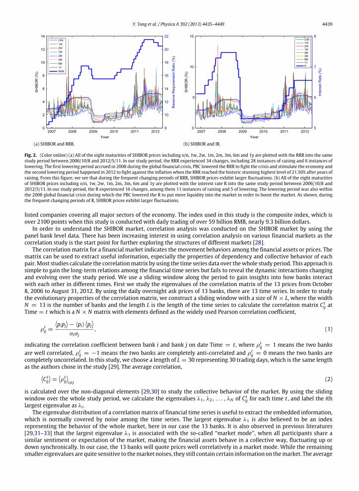
The daily data of SHIBOR-RRR and SHIBOR-R in our study period between 2006 and 2012 are plotted in Fig. 2(a) and (b)respectively. All eight daily SHIBOR rates are plotted which demonstrate a similar shape between RRR and R. Also, we canobserve that the fluctuations of SHIBOR rates are related with the changes of RRR and R, i.e. during changing periods of RRRand R, SHIBOR rates fluctuate significantly, while during non-changing periods, SHIBOR rates are relatively smooth. We alsouse the daily index of the Shanghai stock market (SHSM) to study how the stock market responds to the monetary policychanges. The SHSM index was launched in 1991 with a base value of 100 and constituents for the index are all listed stockson the Shanghai stock market. The SHSM index now represents the fastest growing stock market in the whole world with

Y. Tang et al. / Physica A 392 (2013) 4435–4449 4439

(a) SHIBOR and RRR. (b) SHIBOR and IR.

Fig. 2. (Color online) (a) All of the eight maturities of SHIBOR prices including o/n, 1w, 2w, 1m, 2m, 3m, 6m and 1y are plotted with the RRR into the samestudy period between 2006/10/8 and 2012/5/11. In our study period, the RRR experienced 34 changes, including 28 instances of raising and 6 instances oflowering. The first lowering period accrued in 2008 during the global financial crisis, PBC lowered the RRR to fight the crisis and stimulate the economy andthe second lowering period happened in 2012 to fight against the inflationwhen the RRR reached the historic stunning highest level of 21.50% after years ofraising. From this figure, we see that during the frequent changing periods of RRR, SHIBOR prices exhibit larger fluctuations. (b) All of the eight maturitiesof SHIBOR prices including o/n, 1w, 2w, 1m, 2m, 3m, 6m and 1y are plotted with the interest rate R into the same study period between 2006/10/8 and2012/5/11. In our study period, the R experienced 16 changes, among them 11 instances of raising and 5 of lowering. The lowering period was also withinthe 2008 global financial crisis during which the PBC lowered the R to put more liquidity into the market in order to boost the market. As shown, duringthe frequent changing periods of R, SHIBOR prices exhibit larger fluctuations.

listed companies covering all major sectors of the economy. The index used in this study is the composite index, which isover 2100 points when this study is conducted with daily trading of over 59 billion RMB, nearly 9.3 billion dollars.

In order to understand the SHIBOR market, correlation analysis was conducted on the SHIBOR market by using thepanel bank level data. There has been increasing interest in using correlation analysis on various financial markets as thecorrelation study is the start point for further exploring the structures of different markets [28].

The correlationmatrix for a financial market indicates the movement behaviors among the financial assets or prices. Thematrix can be used to extract useful information, especially the properties of dependency and collective behavior of eachpair. Most studies calculate the correlationmatrix by using the time series data over thewhole study period. This approach issimple to gain the long-term relations among the financial time series but fails to reveal the dynamic interactions changingand evolving over the study period. We use a sliding window along the period to gain insights into how banks interactwith each other in different times. First we study the eigenvalues of the correlation matrix of the 13 prices from October8, 2006 to August 31, 2012. By using the daily overnight ask prices of 13 banks, there are 13 time series. In order to studythe evolutionary properties of the correlation matrix, we construct a sliding window with a size of N × L, where the widthN = 13 is the number of banks and the length L is the length of the time series to calculate the correlation matrix C t

ij atTime = t which is a N × N matrix with elements defined as the widely used Pearson correlation coefficient,

ρtij =

pipj

− ⟨pi⟩

pj

σiσj

, (1)

indicating the correlation coefficient between bank i and bank j on date Time = t , where ρtij = 1 means the two banks

are well correlated, ρtij = −1 means the two banks are completely anti-correlated and ρt

ij = 0 means the two banks arecompletely uncorrelated. In this study, we choose a length of L = 30 representing 30 trading days, which is the same lengthas the authors chose in the study [29]. The average correlation,

C tij

=

ρtij

i=j

(2)

is calculated over the non-diagonal elements [29,30] to study the collective behavior of the market. By using the slidingwindow over the whole study period, we calculate the eigenvalues λ1, λ2, . . . , λN of C t

ij for each time t , and label the ithlargest eigenvalue as λi.

The eigenvalue distribution of a correlationmatrix of financial time series is useful to extract the embedded information,which is normally covered by noise among the time series. The largest eigenvalue λ1 is also believed to be an indexrepresenting the behavior of the whole market, here in our case the 13 banks. It is also observed in previous literatures[29,31–33] that the largest eigenvalue λ1 is associated with the so-called ‘‘market mode’’, when all participants share asimilar sentiment or expectation of the market, making the financial assets behave in a collective way, fluctuating up ordown synchronically. In our case, the 13 banks will quote prices well correlatively in a market mode. While the remainingsmaller eigenvalues are quite sensitive to themarket noises, they still contain certain information on themarket. The average

4440 Y. Tang et al. / Physica A 392 (2013) 4435–4449

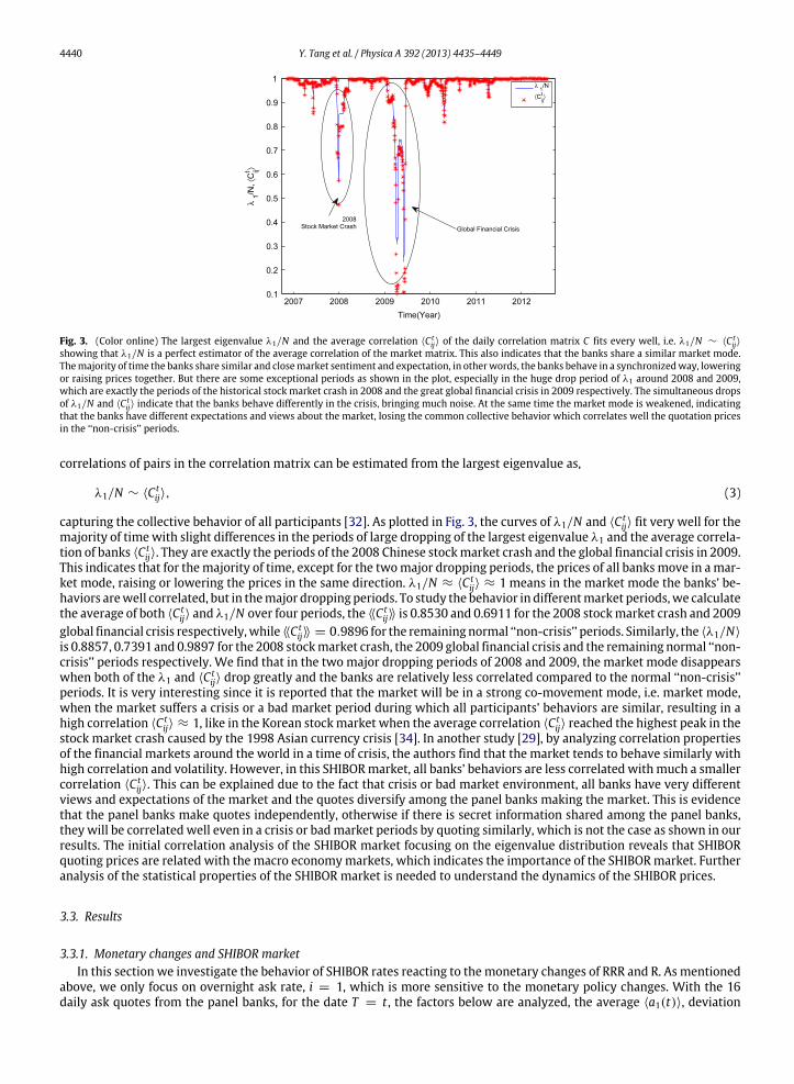
Fig. 3. (Color online) The largest eigenvalue λ1/N and the average correlation ⟨C tij⟩ of the daily correlation matrix C fits every well, i.e. λ1/N ∼ ⟨C t

ij⟩

showing that λ1/N is a perfect estimator of the average correlation of the market matrix. This also indicates that the banks share a similar market mode.Themajority of time the banks share similar and closemarket sentiment and expectation, in otherwords, the banks behave in a synchronizedway, loweringor raising prices together. But there are some exceptional periods as shown in the plot, especially in the huge drop period of λ1 around 2008 and 2009,which are exactly the periods of the historical stock market crash in 2008 and the great global financial crisis in 2009 respectively. The simultaneous dropsof λ1/N and ⟨C t

ij⟩ indicate that the banks behave differently in the crisis, bringing much noise. At the same time the market mode is weakened, indicatingthat the banks have different expectations and views about the market, losing the common collective behavior which correlates well the quotation pricesin the ‘‘non-crisis’’ periods.

correlations of pairs in the correlation matrix can be estimated from the largest eigenvalue as,

λ1/N ∼ ⟨C tij⟩, (3)

capturing the collective behavior of all participants [32]. As plotted in Fig. 3, the curves of λ1/N and ⟨C tij⟩ fit very well for the

majority of timewith slight differences in the periods of large dropping of the largest eigenvalue λ1 and the average correla-tion of banks ⟨C t

ij⟩. They are exactly the periods of the 2008 Chinese stockmarket crash and the global financial crisis in 2009.This indicates that for themajority of time, except for the twomajor dropping periods, the prices of all banksmove in amar-ket mode, raising or lowering the prices in the same direction. λ1/N ≈ ⟨C t

ij⟩ ≈ 1 means in the market mode the banks’ be-haviors arewell correlated, but in themajor dropping periods. To study the behavior in differentmarket periods,we calculatethe average of both ⟨C t

ij⟩ and λ1/N over four periods, the ⟨⟨C tij⟩⟩ is 0.8530 and 0.6911 for the 2008 stockmarket crash and 2009

global financial crisis respectively,while ⟨⟨C tij⟩⟩ = 0.9896 for the remaining normal ‘‘non-crisis’’ periods. Similarly, the ⟨λ1/N⟩

is 0.8857, 0.7391 and 0.9897 for the 2008 stockmarket crash, the 2009 global financial crisis and the remaining normal ‘‘non-crisis’’ periods respectively. We find that in the two major dropping periods of 2008 and 2009, the market mode disappearswhen both of the λ1 and ⟨C t

ij⟩ drop greatly and the banks are relatively less correlated compared to the normal ‘‘non-crisis’’periods. It is very interesting since it is reported that the market will be in a strong co-movement mode, i.e. market mode,when the market suffers a crisis or a bad market period during which all participants’ behaviors are similar, resulting in ahigh correlation ⟨C t

ij⟩ ≈ 1, like in the Korean stockmarket when the average correlation ⟨C tij⟩ reached the highest peak in the

stock market crash caused by the 1998 Asian currency crisis [34]. In another study [29], by analyzing correlation propertiesof the financial markets around the world in a time of crisis, the authors find that the market tends to behave similarly withhigh correlation and volatility. However, in this SHIBORmarket, all banks’ behaviors are less correlated withmuch a smallercorrelation ⟨C t

ij⟩. This can be explained due to the fact that crisis or bad market environment, all banks have very differentviews and expectations of the market and the quotes diversify among the panel banks making the market. This is evidencethat the panel banks make quotes independently, otherwise if there is secret information shared among the panel banks,they will be correlated well even in a crisis or badmarket periods by quoting similarly, which is not the case as shown in ourresults. The initial correlation analysis of the SHIBOR market focusing on the eigenvalue distribution reveals that SHIBORquoting prices are related with the macro economymarkets, which indicates the importance of the SHIBORmarket. Furtheranalysis of the statistical properties of the SHIBOR market is needed to understand the dynamics of the SHIBOR prices.

3.3. Results

3.3.1. Monetary changes and SHIBOR marketIn this section we investigate the behavior of SHIBOR rates reacting to themonetary changes of RRR and R. As mentioned

above, we only focus on overnight ask rate, i = 1, which is more sensitive to the monetary policy changes. With the 16daily ask quotes from the panel banks, for the date T = t , the factors below are analyzed, the average ⟨a1(t)⟩, deviation

Y. Tang et al. / Physica A 392 (2013) 4435–4449 4441

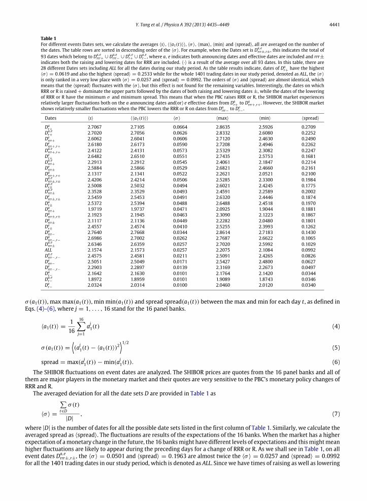
Table 1For different events Dates sets, we calculate the averages ⟨s⟩, ⟨⟨a1(t)⟩⟩, ⟨σ ⟩, ⟨max⟩, ⟨min⟩ and ⟨spread⟩, all are averaged on the number ofthe dates. The table rows are sorted in descending order of the ⟨σ ⟩. For example, when the Dates set is Da,e

rrr±,r± , this indicates the total of93 dates which belong to Da,e

rrr+ ∪ Da,errr− ∪ Da,e

r+ ∪ Da,er− , where a, e indicates both announcing dates and effective dates are included and rrr±

indicates both the raising and lowering dates for RRR are included. ⟨·⟩ is a result of the average over all 93 dates. In this table, there are28 different Dates sets including ALL for all the dates during our study period. As the table results indicate, dates of Da

r+ have the highest⟨σ ⟩ = 0.0619 and also the highest ⟨spread⟩ = 0.2533 while for the whole 1401 trading dates in our study period, denoted as ALL, the ⟨σ ⟩

is only ranked in a very low place with ⟨σ ⟩ = 0.0257 and ⟨spread⟩ = 0.0992. The orders of ⟨σ ⟩ and ⟨spread⟩ are almost identical, whichmeans that the ⟨spread⟩ fluctuates with the ⟨σ ⟩, but this effect is not found for the remaining variables. Interestingly, the dates on whichRRR or R is raised + dominate the upper parts followed by the dates of both raising and lowering dates ±, while the dates of the loweringof RRR or R have the minimum σ and minimum spread. This means that when the PBC raises RRR or R, the SHIBOR market experiencesrelatively larger fluctuations both on the a announcing dates and(or) e effective dates from Da

r+ to Darrr+,r+ . However, the SHIBOR market

shows relatively smaller fluctuations when the PBC lowers the RRR or R on dates from Darrr− to De

r− .

Dates ⟨s⟩ ⟨⟨a1(t)⟩⟩ ⟨σ ⟩ ⟨max⟩ ⟨min⟩ ⟨spread⟩

Dar+ 2.7067 2.7105 0.0664 2.8635 2.5926 0.2709

Da,er+ 2.7020 2.7056 0.0626 2.8332 2.6080 0.2252

Derrr+ 2.6062 2.6041 0.0606 2.7120 2.4630 0.2490

Derrr+,r+ 2.6180 2.6173 0.0590 2.7208 2.4946 0.2262

Da,errr+,r+ 2.4122 2.4131 0.0573 2.5329 2.3082 0.2247

Der+ 2.6482 2.6510 0.0551 2.7435 2.5753 0.1681

Da,errr+ 2.2913 2.2912 0.0545 2.4061 2.1847 0.2214

Derrr± 2.5884 2.5866 0.0529 2.6821 2.4660 0.2161

Darrr+,r+ 2.1317 2.1341 0.0522 2.2621 2.0521 0.2100

Da,errr±,r± 2.4206 2.4214 0.0506 2.5285 2.3300 0.1984

Da,er± 2.5008 2.5032 0.0494 2.6021 2.4245 0.1775

Da,errr± 2.3528 2.3529 0.0493 2.4591 2.2589 0.2002

Derrr±,r± 2.5459 2.5453 0.0491 2.6320 2.4446 0.1874

Dar± 2.5372 2.5394 0.0488 2.6488 2.4518 0.1970

Darrr+ 1.9719 1.9737 0.0471 2.0925 1.9044 0.1881

Darrr±,r± 2.1923 2.1945 0.0463 2.3090 2.1223 0.1867

Darrr± 2.1117 2.1136 0.0449 2.2282 2.0480 0.1801

Der± 2.4557 2.4574 0.0410 2.5255 2.3993 0.1262

Darrr− 2.7640 2.7668 0.0344 2.8614 2.7183 0.1430

Darrr−,r− 2.6986 2.7002 0.0262 2.7687 2.6622 0.1065

Da,errr± 2.6346 2.6359 0.0257 2.7020 2.5992 0.1029

ALL 2.1574 2.1573 0.0257 2.2075 2.1084 0.0992Da,errr−,r− 2.4575 2.4581 0.0211 2.5091 2.4265 0.0826

Derrr− 2.5051 2.5049 0.0171 2.5427 2.4800 0.0627

Derrr−,r− 2.2903 2.2897 0.0139 2.3169 2.2673 0.0497

Dar− 2.1642 2.1630 0.0101 2.1764 2.1420 0.0344

Da,er− 1.8972 1.8959 0.0101 1.9089 1.8743 0.0346

Der− 2.0324 2.0314 0.0100 2.0460 2.0120 0.0340

σ(a1(t)), max max(a1(t)), min min(a1(t)) and spread spread(a1(t)) between the max and min for each day t , as defined inEqs. (4)–(6), where j = 1, . . . , 16 stand for the 16 panel banks.

⟨a1(t)⟩ =116

16j=1

aj1(t) (4)

σ(a1(t)) =

(aj1(t) − ⟨a1(t)⟩)2

1/2(5)

spread = max(aj1(t)) − min(aj1(t)). (6)

The SHIBOR fluctuations on event dates are analyzed. The SHIBOR prices are quotes from the 16 panel banks and all ofthem are major players in the monetary market and their quotes are very sensitive to the PBC’s monetary policy changes ofRRR and R.

The averaged deviation for all the date sets D are provided in Table 1 as

⟨σ ⟩ =

t∈D

σ(t)

|D|, (7)

where |D| is the number of dates for all the possible date sets listed in the first column of Table 1. Similarly, we calculate theaveraged spread as ⟨spread⟩. The fluctuations are results of the expectations of the 16 banks. When the market has a higherexpectation of amonetary change in the future, the 16 banksmight have different levels of expectations and thismightmeanhigher fluctuations are likely to appear during the preceding days for a change of RRR or R. As we shall see in Table 1, on allevent dates Da,e

rrr±,r±, the ⟨σ ⟩ = 0.0501 and ⟨spread⟩ = 0.1963 are almost twice the ⟨σ ⟩ = 0.0257 and ⟨spread⟩ = 0.0992for all the 1401 trading dates in our study period, which is denoted as ALL. Since we have times of raising as well as lowering

4442 Y. Tang et al. / Physica A 392 (2013) 4435–4449

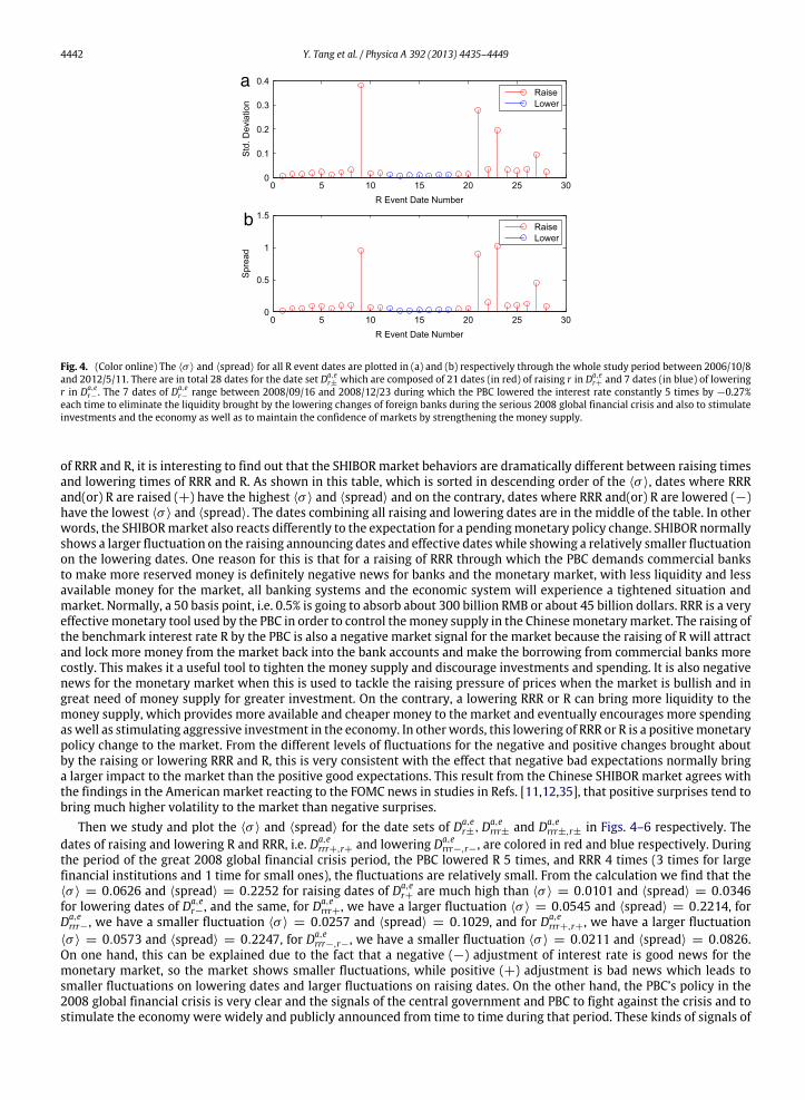
Fig. 4. (Color online) The ⟨σ ⟩ and ⟨spread⟩ for all R event dates are plotted in (a) and (b) respectively through the whole study period between 2006/10/8and 2012/5/11. There are in total 28 dates for the date set Da,e

r± which are composed of 21 dates (in red) of raising r in Da,er+ and 7 dates (in blue) of lowering

r in Da,er− . The 7 dates of Da,e

r− range between 2008/09/16 and 2008/12/23 during which the PBC lowered the interest rate constantly 5 times by −0.27%each time to eliminate the liquidity brought by the lowering changes of foreign banks during the serious 2008 global financial crisis and also to stimulateinvestments and the economy as well as to maintain the confidence of markets by strengthening the money supply.

of RRR and R, it is interesting to find out that the SHIBORmarket behaviors are dramatically different between raising timesand lowering times of RRR and R. As shown in this table, which is sorted in descending order of the ⟨σ ⟩, dates where RRRand(or) R are raised (+) have the highest ⟨σ ⟩ and ⟨spread⟩ and on the contrary, dates where RRR and(or) R are lowered (−)have the lowest ⟨σ ⟩ and ⟨spread⟩. The dates combining all raising and lowering dates are in the middle of the table. In otherwords, the SHIBORmarket also reacts differently to the expectation for a pendingmonetary policy change. SHIBOR normallyshows a larger fluctuation on the raising announcing dates and effective dates while showing a relatively smaller fluctuationon the lowering dates. One reason for this is that for a raising of RRR through which the PBC demands commercial banksto make more reserved money is definitely negative news for banks and the monetary market, with less liquidity and lessavailable money for the market, all banking systems and the economic system will experience a tightened situation andmarket. Normally, a 50 basis point, i.e. 0.5% is going to absorb about 300 billion RMB or about 45 billion dollars. RRR is a veryeffectivemonetary tool used by the PBC in order to control themoney supply in the Chinesemonetarymarket. The raising ofthe benchmark interest rate R by the PBC is also a negative market signal for the market because the raising of R will attractand lock more money from the market back into the bank accounts and make the borrowing from commercial banks morecostly. This makes it a useful tool to tighten the money supply and discourage investments and spending. It is also negativenews for the monetary market when this is used to tackle the raising pressure of prices when the market is bullish and ingreat need of money supply for greater investment. On the contrary, a lowering RRR or R can bring more liquidity to themoney supply, which provides more available and cheaper money to the market and eventually encourages more spendingaswell as stimulating aggressive investment in the economy. In otherwords, this lowering of RRR or R is a positivemonetarypolicy change to the market. From the different levels of fluctuations for the negative and positive changes brought aboutby the raising or lowering RRR and R, this is very consistent with the effect that negative bad expectations normally bringa larger impact to the market than the positive good expectations. This result from the Chinese SHIBOR market agrees withthe findings in the American market reacting to the FOMC news in studies in Refs. [11,12,35], that positive surprises tend tobring much higher volatility to the market than negative surprises.

Then we study and plot the ⟨σ ⟩ and ⟨spread⟩ for the date sets of Da,er±,Da,e

rrr± and Da,errr±,r± in Figs. 4–6 respectively. The

dates of raising and lowering R and RRR, i.e. Da,errr+,r+ and lowering Da,e

rrr−,r−, are colored in red and blue respectively. Duringthe period of the great 2008 global financial crisis period, the PBC lowered R 5 times, and RRR 4 times (3 times for largefinancial institutions and 1 time for small ones), the fluctuations are relatively small. From the calculation we find that the⟨σ ⟩ = 0.0626 and ⟨spread⟩ = 0.2252 for raising dates of Da,e

r+ are much high than ⟨σ ⟩ = 0.0101 and ⟨spread⟩ = 0.0346for lowering dates of Da,e

r−, and the same, for Da,errr+, we have a larger fluctuation ⟨σ ⟩ = 0.0545 and ⟨spread⟩ = 0.2214, for

Da,errr−, we have a smaller fluctuation ⟨σ ⟩ = 0.0257 and ⟨spread⟩ = 0.1029, and for Da,e

rrr+,r+, we have a larger fluctuation⟨σ ⟩ = 0.0573 and ⟨spread⟩ = 0.2247, for Da,e

rrr−,r−, we have a smaller fluctuation ⟨σ ⟩ = 0.0211 and ⟨spread⟩ = 0.0826.On one hand, this can be explained due to the fact that a negative (−) adjustment of interest rate is good news for themonetary market, so the market shows smaller fluctuations, while positive (+) adjustment is bad news which leads tosmaller fluctuations on lowering dates and larger fluctuations on raising dates. On the other hand, the PBC’s policy in the2008 global financial crisis is very clear and the signals of the central government and PBC to fight against the crisis and tostimulate the economy were widely and publicly announced from time to time during that period. These kinds of signals of

Y. Tang et al. / Physica A 392 (2013) 4435–4449 4443

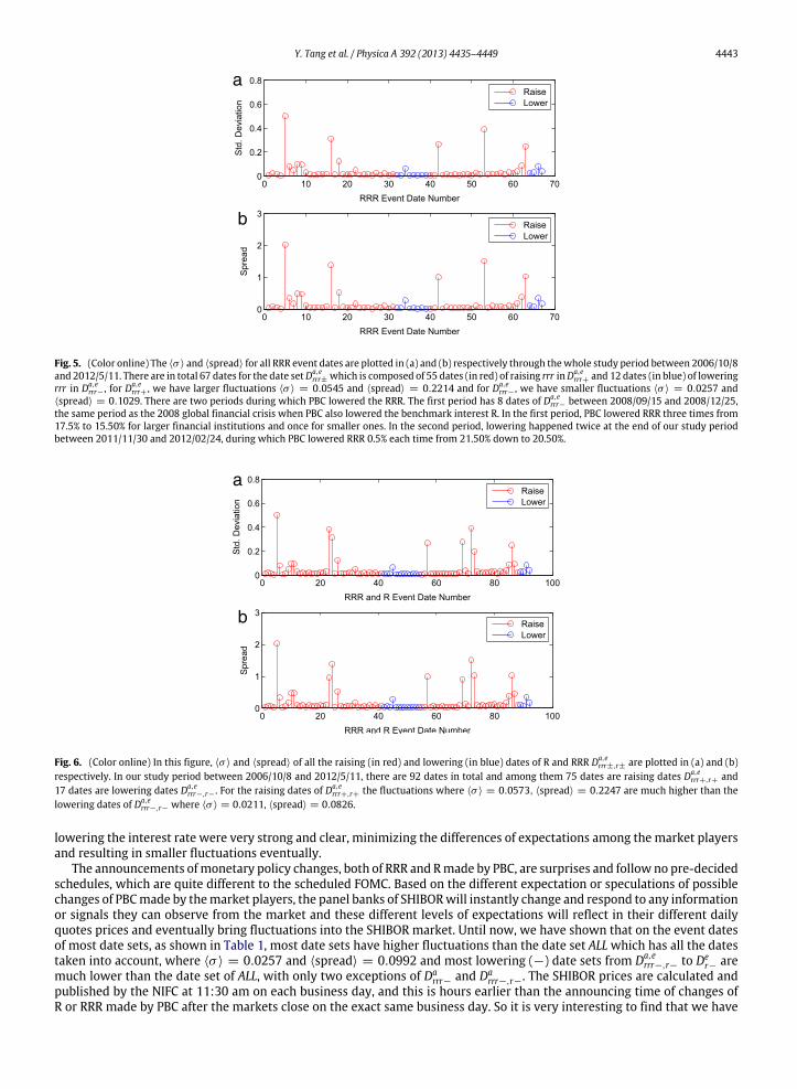
Fig. 5. (Color online) The ⟨σ ⟩ and ⟨spread⟩ for all RRR event dates are plotted in (a) and (b) respectively through thewhole study period between 2006/10/8and 2012/5/11. There are in total 67 dates for the date setDa,e

rrr± which is composed of 55 dates (in red) of raising rrr inDa,errr+ and 12 dates (in blue) of lowering

rrr in Da,errr− , for Da,e

rrr+ , we have larger fluctuations ⟨σ ⟩ = 0.0545 and ⟨spread⟩ = 0.2214 and for Da,errr− , we have smaller fluctuations ⟨σ ⟩ = 0.0257 and

⟨spread⟩ = 0.1029. There are two periods during which PBC lowered the RRR. The first period has 8 dates of Da,errr− between 2008/09/15 and 2008/12/25,

the same period as the 2008 global financial crisis when PBC also lowered the benchmark interest R. In the first period, PBC lowered RRR three times from17.5% to 15.50% for larger financial institutions and once for smaller ones. In the second period, lowering happened twice at the end of our study periodbetween 2011/11/30 and 2012/02/24, during which PBC lowered RRR 0.5% each time from 21.50% down to 20.50%.

Fig. 6. (Color online) In this figure, ⟨σ ⟩ and ⟨spread⟩ of all the raising (in red) and lowering (in blue) dates of R and RRR Da,errr±,r± are plotted in (a) and (b)

respectively. In our study period between 2006/10/8 and 2012/5/11, there are 92 dates in total and among them 75 dates are raising dates Da,errr+,r+ and

17 dates are lowering dates Da,errr−,r− . For the raising dates of Da,e

rrr+,r+ the fluctuations where ⟨σ ⟩ = 0.0573, ⟨spread⟩ = 0.2247 are much higher than thelowering dates of Da,e

rrr−,r− where ⟨σ ⟩ = 0.0211, ⟨spread⟩ = 0.0826.

lowering the interest rate were very strong and clear, minimizing the differences of expectations among the market playersand resulting in smaller fluctuations eventually.

The announcements ofmonetary policy changes, both of RRR and Rmade by PBC, are surprises and follow no pre-decidedschedules, which are quite different to the scheduled FOMC. Based on the different expectation or speculations of possiblechanges of PBCmade by themarket players, the panel banks of SHIBORwill instantly change and respond to any informationor signals they can observe from the market and these different levels of expectations will reflect in their different dailyquotes prices and eventually bring fluctuations into the SHIBOR market. Until now, we have shown that on the event datesof most date sets, as shown in Table 1, most date sets have higher fluctuations than the date set ALLwhich has all the datestaken into account, where ⟨σ ⟩ = 0.0257 and ⟨spread⟩ = 0.0992 and most lowering (−) date sets from Da,e

rrr−,r− to Der− are

much lower than the date set of ALL, with only two exceptions of Darrr− and Da

rrr−,r−. The SHIBOR prices are calculated andpublished by the NIFC at 11:30 am on each business day, and this is hours earlier than the announcing time of changes ofR or RRR made by PBC after the markets close on the exact same business day. So it is very interesting to find that we have

4444 Y. Tang et al. / Physica A 392 (2013) 4435–4449

significantly different, relatively higher (raising +) and smaller (lowering −) fluctuations on the date sets on which RRRand/or R are changed by PBC compared to the whole date set ALL in our study period. This indicates that the SHIBORmarkethas a certain predictive ability of a potential monetary change.

We have investigated how the SHIBORmarket responds on event dates, the next step is to study how the SHIBOR changesbefore and after an event date, either for R or RRR, and also to study how it might behave differently between announcingdates (Time = 0) of Da

rrr±,r± and effective dates of Derrr±,r±. To do this, we study a time window around the event date, we

take a window size of 11 working days, in other words, we include the 5 days before and after the event date respectively.We calculate the averaged ⟨σ ⟩, the fluctuations, for the ith day, which we obtain from the following equation,

⟨σi⟩ =

t∈D,t=i

σ(t)

|D|, (8)

where i = −5 · · · 5, for each date of the date sets and plot the results of raising ones (+) in red, lowering ones (−) in green,and all raising–lowering ones (±) in blue, as shown in Fig. 7(a)–(f). In Fig. 7(a), 16 times of the announcing of changes ofR are averaged for raising (+, in red), lowering (−, in green) and both of raising and lowering (±, in blue) respectively.From this window study, we find that for all of the six sets, there are two significant interesting effects: (1) ‘‘Sign effect’’.The averaged fluctuations ⟨σ ⟩ for raising R or(and) RRR (in red) are always higher the lowering R or(and) RRR (in green),while the fluctuation of raising and lowering dates (in blue) lies between the two of them. This is also consistent withthe ‘‘sign effect’’ that negative changes of monetary policy (raising R or RRR) has a larger influence on the market thanthe positive changes (lowering R or RRR) [11,12,25,35]. (2) Leading fluctuation effect. We find that during the period ofTime = [−5, . . . ,−1] before the announcing date Time = 0, the fluctuation has a significant climbing process leadingto the period of Time = [−5, . . . , 0] before the event dates where Time = 0 for the announcing dates Da in (a), (c)and (e). The fluctuation reaches the highest peak on the dates one day before the announcing dates, Time = −1, for Rchanges in Da

r±, on the announcing dates, Time = 0, for RRR changes in Darrr±, and again on the dates one day before the

announcing dates, Time = −1, for R–RRR changes in Darrr±,r±. This effect shows that the SHIBOR market has a certain

predictability regarding upcomingmonetary policy changes, otherwise the fluctuation should not have an obvious climbingprocess and reach peaks before the announcing day. In other words, it might be possible that the commercial banks keepwatching the market environment very carefully and any acts of the PBC sensing a PBC’s upcoming monetary change mightbe due in order to reduce climbing inflation rates or to provide money supply into the market. It looks like the commercialbanks have a certain collective intelligence that can predict an upcoming change. The PBC’s sudden monetary changes arekept secret and would only be made public when they are released through the official announcements. We cannot tellthe reason from the data, but the results show that the SHIBOR market is a good place to monitor the possible monetarychanges, and the obtaining of a higher fluctuation before the announcing date is a result of the different sentiments of thecommercial banks regarding the monetary markets. This stylized fact is a very interesting finding of the empirical study ofthe SHIBOR fluctuation behavior. It is also known that if there is a lead or lag between financial markets, there might besome opportunity to take advantage of these kinds of lead or lag time gaps to design a profitable trading strategy [36]. Butit still needs comprehensive study and testing before any applications can be used.

3.3.2. Monetary changes and Shanghai stock marketWe have investigated the response of SHIBOR market to the monetary policy changes in the previous sections, now

we focus on how the stock market might be influenced by the monetary changes of R and RRR. As we have mentionedbefore, most previous studies use stock market data, especially the S&P500 index prices data to study the impact of FEDpolicy changes [5,6,8,11,37–39]. The S&P500 index and stock prices demonstrate a significant response to monetary policychanges, a price fall is observed after a rise of the FED funds rate [5] and, the empirical study in Ref. [6] reports a larger effecton the S&P500 index in the bear market. In a time widow of 30-min, a negative market response is found regarding theunexpected changes by FOMC [37]. Another study [11] focuses on the implied volatility and argues that a monetary policychange in expansive periods is more influential for both scheduled and unscheduled changes.

The situation in China is quite different from other countries. China is an emerging economy and the stock market isattractingmore andmore attention among the global financial markets, and themonetary policy changes aremadewithoutschedules, unlike the scheduled FOMC of FED. In this section, we use the daily index of the Shanghai stockmarket during thesame study period between 2006-10-08 and 2012-05-11 to study how the stock market is impacted by the policy changesof PBC. We focus on the index return, defined as

Ireturn(t) = ln I(t) − ln I(t − 1), (9)

which is logged daily return. We use an 11-day time window with event dates (Time = 0) in the middle and averagedthe returns for the date sets of Da

r±,Dar±,Da

r± and Dar± to investigate how the stock market can be influenced by different

changes. The averaged return of the ith day of date set D is defined as,

⟨Ireturn,i(t)⟩ =

t∈D,t=i

Ireturn(t)

|D|, (10)

Y. Tang et al. / Physica A 392 (2013) 4435–4449 4445

(a) Dar± . (b) De

r± .

(c) Darrr± . (d) De

rrr± .

(e) Darrr±,r± . (f) De

rrr±,r± .

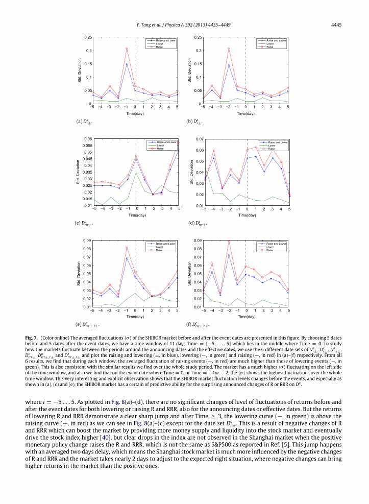
Fig. 7. (Color online) The averaged fluctuations ⟨σ ⟩ of the SHIBORmarket before and after the event dates are presented in this figure. By choosing 5 datesbefore and 5 dates after the event dates, we have a time window of 11 days Time = [−5, . . . , 5] which lies in the middle where Time = 0. To studyhow the markets fluctuate between the periods around the announcing dates and the effective dates, we use the 6 different date sets of Da

r±,Der±,Da

rrr± ,Derrr± , Da

rrr±,r± and Derrr±,r± and plot the raising and lowering (±, in blue), lowering (−, in green) and raising (+, in red) in (a)–(f) respectively. From all

6 results, we find that during each window, the averaged fluctuation of raising events (+, in red) are much higher than those of lowering events (−, ingreen). This is also consistent with the similar results we find over the whole study period. The market has a much higher ⟨σ ⟩ fluctuating on the left sideof the time window, and also we find that on the event date where Time = 0, or Time = −1or − 2, the ⟨σ ⟩ shows the highest fluctuations over the wholetime window. This very interesting and explicit observation shows that the SHIBOR market fluctuation levels changes before the events, and especially asshown in (a), (c) and (e), the SHIBOR market has a certain of predictive ability for the surprising announced changes of R or RRR on Da .

where i = −5 . . . 5. As plotted in Fig. 8(a)–(d), there are no significant changes of level of fluctuations of returns before andafter the event dates for both lowering or raising R and RRR, also for the announcing dates or effective dates. But the returnsof lowering R and RRR demonstrate a clear sharp jump and after Time ≥ 3, the lowering curve (−, in green) is above theraising curve (+, in red) as we can see in Fig. 8(a)–(c) except for the date set Da

r±. This is a result of negative changes of Rand RRR which can boost the market by providing more money supply and liquidity into the stock market and eventuallydrive the stock index higher [40], but clear drops in the index are not observed in the Shanghai market when the positivemonetary policy change raises the R and RRR, which is not the same as S&P500 as reported in Ref. [5]. This jump happenswith an averaged two days delay, whichmeans the Shanghai stockmarket is muchmore influenced by the negative changesof R and RRR and the market takes nearly 2 days to adjust to the expected right situation, where negative changes can bringhigher returns in the market than the positive ones.

4446 Y. Tang et al. / Physica A 392 (2013) 4435–4449

(a) Dar± . (b) De

r± .

(c) Darrr± . (d) De

rrr± .

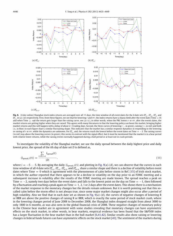
Fig. 8. (Color online) Shanghai stock index returns are averaged over all 11 days, the time window of all event dates for the 4 date sets Dar±,Da

r±,Dar± and

Dar± in (a)–(d) respectively. First, from these figures, we see that for lowering r and rrr , the index returns have a sharp climb after the event date (Time = 0)

and when Time ≥: eq6 the return gets larger than the raising curve, see (a)–(c), in other words, when the PBC lowers r or rrr , after the events dates, themarket returns are getting higher when they are raised. This agrees withmany literatures in that the lowering policy can boost themarket, bringing highermarket returns and this will happen with a delay of about 2–3 trading days. Second, the three curves of lowering (−, in green), raising (+, in red) and both(±, in blue) in each figure share a similar fluctuating shape. This indicates that the market has a similar response dynamics in responding to the loweringor raising of r or rrr , while the dynamics are unknown. For Da

r± and, the returns reach the lowest before the event dates on Time = −3. The raising curves(in red) stay above the lowering curves (in green), this seems in contrast with the signal effect, but it must be mentioned that the market is in a bear periodwith relative lower returns, while the raising events normally happened during a bull period or at least not in crash periods.

To investigate the volatility of the Shanghai market, we use the daily spread between the daily highest price and dailylowest price, the spread of the ith day of date set D is defined as,

⟨Ispread,i(t)⟩ =

t∈D,t=i

Ispread(t)

|D|, (11)

where i = −5 · · · 5. By averaging the daily ⟨Ispread,i(t)⟩ and plotting in Fig. 9(a)–(d), we can observe that the curves in eachtime window of all 4 date sets Da

r±,Der±,Da

rrr± and Derrr± share a similar shape and there is a decline of volatility before event

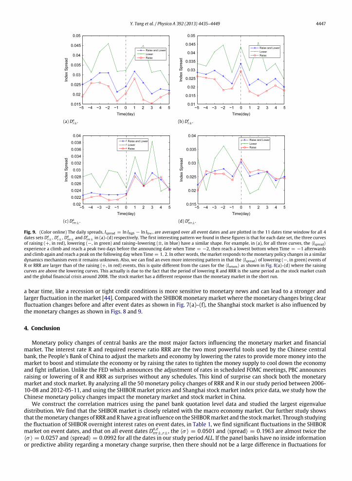
dates where Time = 0 which is agreement with the phenomenon of calm before storm in Ref. [15] of Irish stock market,in which the author reported that there appears to be a decline in volatility on the day prior to an FOMC meeting and asubsequent increase in volatility after the results of the FOMC meeting are made known. The spread reaches a peak onTime = −2, namely two days before the event dates and falls to the lowest point on the day on Time = −1, then followedby a fluctuation and reaching a peak again on Time = 1, 2, 1 or 2 days after the event dates. This shows there is amechanismof the market response to the monetary changes but the details remain unknown. But it is worth pointing out that this so-called calm before the storm effect is not always true, since some major market changes might also occur after a period ofhigh volatility. Also we find that in each date set as shown in Fig. 9(a)–(d), the curves of negative changes of lowering Ror RRR are above the positive changes of raising R or RRR, which is exactly the same period of stock market crash, wherein the lowering changes period of June 2008 to December 2008, the Shanghai index dropped straight from about 3000 toonly 1800 in 6 months, as was also seen in the global financial crisis of 2008. These negative changes of monetary policyin the Chinese bear market are in agreement with some studies revealing that monetary changes can have asymmetriceffects on the stock market, in other words, in bear markets, empirical evidence has been found that the S&P500 indexhas a larger fluctuation in the bear market than in the bull market [6,41,42]. Similar results also show raising or loweringchanges in federal funds futures can have asymmetric effects on the stock market [43]. The sentiment of the markets during

Y. Tang et al. / Physica A 392 (2013) 4435–4449 4447

(a) Dar± . (b) De

r± .

(c) Darrr± . (d) De

rrr± .

Fig. 9. (Color online) The daily spreads, Ispread = ln Ihigh − ln Ilow , are averaged over all event dates and are plotted in the 11 dates time window for all 4dates sets Da

r±,Der±,Da

rrr± and Derrr± in (a)–(d) respectively. The first interesting pattern we found in these figures is that for each date set, the three curves

of raising (+, in red), lowering (−, in green) and raising–lowering (±, in blue) have a similar shape. For example, in (a), for all three curves, the ⟨Ispread⟩experience a climb and reach a peak two days before the announcing date when Time = −2, then reach a lowest bottom when Time = −1 afterwardsand climb again and reach a peak on the following day when Time = 1, 2. In other words, the market responds to the monetary policy changes in a similardynamics mechanism even it remains unknown. Also, we can find an even more interesting pattern in that the ⟨Ispread⟩ of lowering (−, in green) events ofR or RRR are larger than of the raising (+, in red) events, this is quite different from the cases for the ⟨Ireturn⟩ as shown in Fig. 8(a)–(d) where the raisingcurves are above the lowering curves. This actually is due to the fact that the period of lowering R and RRR is the same period as the stock market crashand the global financial crisis around 2008. The stock market has a different response than the monetary market in the short run.

a bear time, like a recession or tight credit conditions is more sensitive to monetary news and can lead to a stronger andlarger fluctuation in themarket [44]. Compared with the SHIBORmonetary market where themonetary changes bring clearfluctuation changes before and after event dates as shown in Fig. 7(a)–(f), the Shanghai stock market is also influenced bythe monetary changes as shown in Figs. 8 and 9.

4. Conclusion

Monetary policy changes of central banks are the most major factors influencing the monetary market and financialmarket. The interest rate R and required reserve ratio RRR are the two most powerful tools used by the Chinese centralbank, the People’s Bank of China to adjust the markets and economy by lowering the rates to provide more money into themarket to boost and stimulate the economy or by raising the rates to tighten the money supply to cool down the economyand fight inflation. Unlike the FED which announces the adjustment of rates in scheduled FOMC meetings, PBC announcesraising or lowering of R and RRR as surprises without any schedules. This kind of surprise can shock both the monetarymarket and stock market. By analyzing all the 50 monetary policy changes of RRR and R in our study period between 2006-10-08 and 2012-05-11, and using the SHIBOR market prices and Shanghai stock market index price data, we study how theChinese monetary policy changes impact the monetary market and stock market in China.

We construct the correlation matrices using the panel bank quotation level data and studied the largest eigenvaluedistribution. We find that the SHIBOR market is closely related with the macro economy market. Our further study showsthat themonetary changes of RRR andRhave a great influence on the SHIBORmarket and the stockmarket. Through studyingthe fluctuation of SHIBOR overnight interest rates on event dates, in Table 1, we find significant fluctuations in the SHIBORmarket on event dates, and that on all event dates Da,e

rrr±,r±, the ⟨σ ⟩ = 0.0501 and ⟨spread⟩ = 0.1963 are almost twice the⟨σ ⟩ = 0.0257 and ⟨spread⟩ = 0.0992 for all the dates in our study period ALL. If the panel banks have no inside informationor predictive ability regarding a monetary change surprise, then there should not be a large difference in fluctuations for

4448 Y. Tang et al. / Physica A 392 (2013) 4435–4449

ALL and Da,errr±,r±. These findings show that the SHIBOR market is very sensitive to the impact of monetary changes of PBC,

and based on the observed behaviors of panel banks, it seems that the SHIBOR market has a certain predictive ability forpotential changes, but this needs more careful study and it would be a worthy topic of further investigation. Also, fromTable 1, we find that the raising of RRR or R leads to larger fluctuations in the SHIBOR market than the lowering changes.This result agrees with the ‘‘sign effect’’ [25,12] in which bad news has a greater impact than good news on the market, inour case, the raising of RRR or R is bad news for the market because this kind of change means the PBC wants to tighten themoney supply and bring larger fluctuations to the market, while the lowering of RRR or R means more liquidity and moneysupply to the market which is good news and brings smaller fluctuations. By constructing an event window with a size of11 trading days, we also study how SHIBOR responds before and after the each monetary change. The averaged fluctuations⟨σ ⟩ of the SHIBOR market before and after the event dates are presented in Fig. 7. We again find clear ‘‘sign effect’’ whereall ⟨σ ⟩ of raising of R or RRR are higher than those of lowering of R or RRR over all date sets from Da

r± to Derrr±,r± as shown

in Fig. 7(a)–(f).The monetary policy changes can also have a great influence on the stock market. In order to study how the changes can

impact the stock market, we use the daily Shanghai index data and build an event time window of the same length to seehow the stock market responds differently before and after the event dates. As plotted in Fig. 8 for the index return andFig. 9 for the volatility respectively, we find that the market returns will climb up with about a 3 day delay in the Shanghaistock market after the lowering monetary changes happen, and this is agreement with the effect that a market friendlypolicy, i.e. lowering the rate providing more money to the market, will bring about high returns. However, this will nothappen immediately, but only with about a 3 day delay on average which indicates that the stock market slowly digeststhe monetary policy impact and reacts correctly. Also, we find that the volatilities of the Shanghai market, indicated as adaily spread of index return, as shown in Fig. 9, are influenced by the changes differently from the SHIBORmonetary markettoo. In the stock market, the volatilities of lowering changes are larger than that of raising changes, while for the SHIBORmarket, the fluctuations of SHIBOR prices are the opposite, that raising R or RRR will bring larger fluctuations than loweringthe rates. The reason behind this is that the period when PBC lowered the R or RRR was actually the bear market period ofaround 2008 when the market experienced a large crash. This is actually in agreement with previous studies, which foundmonetary policy changes during bad times or in a bear market might lead to larger volatility and fluctuations in the stockmarket [6,12,41,42].

Recently, many studies have emphasized the applicability and how the empirical findings can be valuable for policymak-ers [45]. Here we show that monetary policymakers must pay serious attention to how both themonetary market and stockmarket are impacted by the monetary policy changes [46], especially in a country like China where the economy is boom-ing and the monetary changes are announced to the market as surprises with no pre-decided schedules. The stock marketfluctuation is determined by the demand and supply shocks as well as themonetary policy changes [3], the findings suggestthat in the short run timewindow ofmonetary changes, themarket is influenced by the changes and demonstrates differentbehaviors in bear and bull markets to differentmonetary policies, either lowering or raising RRR and R. PBC is responsible forsetting theR andRRR and it plays the same role as FED,which attractedmuch criticism for not doing enough to keep the econ-omy healthy or even causing bubbles [47]. The empirical studies revealedwould be useful to understand the relationship be-tween themarket and policy changes, and are also useful for the policymakers tomonitor and evaluate the effect ofmonetarychanges to the monetary market and stock market, since the stock market is a monetary policy transmission channel [23].

Acknowledgments

We thank the anonymous reviewers for their comments and suggestions, which helped us improve this work. We alsowish to thank Liang Zhang for interesting discussions, and we are thankful for the financial support from National ScienceFoundation of China under grant No. 71172095 and Ministry of Science and Technology of the People’s Republic of Chinaunder grant No. 2011IM020100.

References

[1] P. Sellin, Monetary policy and the stock market: theory and empirical evidence, Journal of Economic Surveys 15 (2001) 491–541.[2] M. Farka, The effect of monetary policy shocks on stock prices accounting for endogeneity and omitted variable biases, Review of Financial Economics

18 (2009) 47–55.[3] D. Du, Monetary policy, stock returns and inflation, Journal of Economics and Business 58 (2006) 36–54.[4] L.T. He, Variations in effects of monetary policy on stock market returns in the past four decades, Review of Financial Economics 15 (2006) 331–349.[5] H.C. Bjørnland, K. Leitemo, Identifying the interdependence between US monetary policy and the stock market, Journal of Monetary Economics 56

(2009) 275–282.[6] S.-S. Chen, Doesmonetary policy have asymmetric effects on stock returns? Journal of Money, Credit & Banking 39 (2007) 667–688 (Wiley-Blackwell).[7] N. Gospodinov, I. Jamali, The effects of federal funds rate surprises on S&P 500 volatility and volatility risk premium, Journal of Empirical Finance 19

(2012) 497–510.[8] B.T. Ewing, Monetary policy and stock returns, Bulletin of Economic Research 53 (2001) 73.[9] J. Scharler, Bank lending and the stock market’s response to monetary policy shocks, International Review of Economics and Finance 17 (2008)

425–435.[10] W. Thorbecke, On stock market returns and monetary policy, Journal of Finance 52 (1997) 635–654.[11] S. Vähämaa, J. Äijö, The Fed’s policy decisions and implied volatility, Journal of Futures Markets 31 (2011) 995–1010.[12] A.M. Petersen, F. Wang, S. Havlin, H.E. Stanley, Quantitative law describing market dynamics before and after interest-rate change, Physical Review E

81 (2010) 066121.

Y. Tang et al. / Physica A 392 (2013) 4435–4449 4449

[13] A.M. Petersen, F. Wang, S. Havlin, H.E. Stanley, Market dynamics immediately before and after financial shocks: quantifying the Omori, productivity,and Bath laws, Physical Review E 82 (2010) 036114.

[14] F. Allen, Financial structure and financial crisis, International Review of Finance 2 (2001) 1–19.[15] D. Bredin, C. Gavin, G. O’Reilly, US monetary policy announcements and Irish stock market volatility, Applied Financial Economics 15 (2005)

1243–1250.[16] D. Bredin, S. Hyde, D. Nitzsche, G. O’Reilly, European monetary policy surprises: the aggregate and sectoral stock market response, International

Journal of Finance & Economics 14 (2009) 156–171.[17] N. Cassola, C. Morana, Monetary policy and the stock market in the euro area, Journal of Policy Modeling 26 (2004) 387–399.[18] O. Fernandez-Amador, M. Gächter, M. Larch, G. Peter, Monetary policy and its impact on stockmarket liquidity: evidence from the euro zone,Working

Papers, Faculty of Economics and Statistics, University of Innsbruck, February 2011.[19] S.M. Hussain, Simultaneous monetary policy announcements and international stock markets response: an intraday analysis, Journal of Banking &

Finance 35 (2011) 752–764. Australasian finance conference: global financial crisis, international financial architecture and regulation.[20] K. Kholodilin, A. Montagnoli, O. Napolitano, B. Siliverstovs, Assessing the impact of the ECB’s monetary policy on the stock markets: a sectoral view,

Economics Letters 105 (2009) 211–213.[21] C. Ioannidis, A. Kontonikas, The impact of monetary policy on stock prices, Journal of Policy Modeling 30 (2008) 33–53.[22] Y.D. Li, T.B. Iscan, K. Xu, The impact of monetary policy shocks on stock prices: evidence from Canada and the United States, Journal of International

Money and Finance 29 (2010) 876–896.[23] J.B. Durham, The effect of monetary policy on monthly and quarterly stock market returns: cross-country evidence and sensitivity analyses, in: Board

of Governors of the Federal Reserve System, (US), in: Finance and Economics Discussion Series, 2001.[24] D. Dickinson, J. Liu, The real effects of monetary policy in China: an empirical analysis, China Economic Review 18 (2007) 87–111.[25] T.G. Andersen, T. Bollerslev, F.X. Diebold, C. Vega, Micro effects of macro announcements: real-time price discovery in foreign exchange, American

Economic Review 93 (2003) 38–62.[26] Monetary policy of the people’s bank of China, July 2012. http://www.pbc.gov.cn/publish/english/957/index.html.[27] Shanghai Interbank Offered Rate (SHIBOR) of Chinese Commercial Banks, July 2012. http://www.shibor.org.[28] R. Mantegna, Hierarchical structure in financial markets, The European Physical Journal B—Condensed Matter and Complex Systems 11 (1999)

193–197.[29] L.S. Junior, I.D.P. Franca, Correlation of financial markets in times of crisis, Physica A: Statistical Mechanics and its Applications 391 (2012) 187–208.[30] D.-M. Song, M. Tumminello, W.-X. Zhou, R.N. Mantegna, Evolution of worldwide stock markets, correlation structure, and correlation-based graphs,

Physical Review E 84 (2011) 026108.[31] G. Livan, L. Rebecchi, Asymmetric correlationmatrices: an analysis of financial data, The European Physical Journal B—CondensedMatter and Complex

Systems 85 (2012) 1–11.[32] G. Tilak, T. Széll, R. Chicheportiche, A. Chakraborti, Study of statistical correlations in intraday and daily financial return time series, in: F. Abergel,

B.K. Chakrabarti, A. Chakraborti, A. Ghosh (Eds.), Econophysics of Systemic Risk and Network Dynamics, in: New EconomicWindows, Springer, Milan,2013, pp. 77–104.

[33] L. Sandoval Junior, Cluster formation and evolution in networks of financial market indices. ArXiv e-prints arXiv:1111.5069.[34] G. Oh, C. Eom, F. Wang, W.-S. Jung, H.E. Stanley, S. Kim, Statistical properties of cross-correlation in the Korean stock market, The European Physical

Journal B 79 (2011) 55–60.[35] A.N. Bomfim, Pre-announcement effects, news effects, and volatility: Monetary policy and the stock market, Journal of Banking & Finance 27 (2003)

133–151.[36] M.S. Rozeff, Money and stock prices: market efficiency and the lag in effect of monetary policy, Journal of Financial Economics 1 (1974) 245–302.[37] T. Davig, J.R. Gerlach, State-dependent stock market reactions to monetary policy, International Journal of Central Banking 2 (2006) 65–83.[38] M. Ehrmann, M. Fratzscher, Taking stock: monetary policy transmission to equity markets, Journal of Money, Credit & Banking 36 (2004) 719–737

(Ohio State University Press).[39] T. Mann, R.J. Atra, R. Dowen, US monetary policy indicators and international stock returns: 1970–2001, International Review of Financial Analysis 13

(2004) 543–558.[40] J. Tobin, A general equilibrium approach to monetary theory, Journal of Money, Credit and Banking 1 (1969) 15–29.[41] D.W. Jansen, C.-L. Tsai, Monetary policy and stock returns: financing constraints and asymmetries in bull and bear markets, Journal of Empirical

Finance 17 (2010) 981–990.[42] A. Kurov, Investor sentiment and the stock market’s reaction to monetary policy, Journal of Banking & Finance 34 (2010) 139–149.[43] O. David Gulley, J. Sultan, The link between monetary policy and stock and bond markets: evidence from the federal funds futures contract, Applied

Financial Economics 13 (2003) 199.[44] A. Basistha, A. Kurov, Macroeconomic cycles and the stock market’s reaction to monetary policy, Journal of Banking & Finance 32 (2008) 2606–2616.[45] B. Podobnik, D. Horvatić, D.Y. Kenett, H.E. Stanley, The competitiveness versus the wealth of a country, Scientific Reports 2 (2012).[46] B. Bernanke, M. Gertler, Monetary policy and asset price volatility, Economic Review 84 (1999) 17–51.[47] S.F. England, The Federal reserve board and the stock market bubble, Business Economics 38 (2003) 33.