impact of optimally placed var support on electricity spot
TRANSCRIPT

Graduate Theses, Dissertations, and Problem Reports
2006
Impact of optimally placed VAR support on electricity spot pricing Impact of optimally placed VAR support on electricity spot pricing
Ramesh Kumar V. Khajjayam West Virginia University
Follow this and additional works at: https://researchrepository.wvu.edu/etd
Recommended Citation Recommended Citation Khajjayam, Ramesh Kumar V., "Impact of optimally placed VAR support on electricity spot pricing" (2006). Graduate Theses, Dissertations, and Problem Reports. 1774. https://researchrepository.wvu.edu/etd/1774
This Thesis is protected by copyright and/or related rights. It has been brought to you by the The Research Repository @ WVU with permission from the rights-holder(s). You are free to use this Thesis in any way that is permitted by the copyright and related rights legislation that applies to your use. For other uses you must obtain permission from the rights-holder(s) directly, unless additional rights are indicated by a Creative Commons license in the record and/ or on the work itself. This Thesis has been accepted for inclusion in WVU Graduate Theses, Dissertations, and Problem Reports collection by an authorized administrator of The Research Repository @ WVU. For more information, please contact [email protected].
Impact of Optimally Placed VAR Support on
Electricity Spot Pricing
by
Ramesh Kumar V. Khajjayam
Thesis submitted to theCollege of Engineering and Mineral Resources
at West Virginia Universityin partial fulfillment of the requirements
for the degree of
Master of Sciencein
Electrical Engineering
Professor Muhammad A. Choudhry, Ph.D.Professor Powsiri Klinkhachorn, Ph.D.
Professor Ali Feliachi, Ph.D., Chair
Lane Department of Computer Science and Electrical Engineering
Morgantown, West Virginia2006
Keywords: Electricity pricing, VAR support, cost benefit analysis, spot prices, N-1contingency criterion, voltage stability constrained OPF, transmission pricing

Abstract
Impact of Optimally Placed VAR Support on Electricity Spot Pricing
by
Ramesh Kumar V. Khajjayam
Master of Science in Electrical Engineering
West Virginia University
Professor Ali Feliachi, Ph.D., Chair
In view of deregulation and privatization processes, electricity pricing becomes one of themost important issues. The increases in power flows and environmental constraints are forcingelectricity utilities to install new VAR equipment to enhance network operation. In this thesisa nonlinear multi-objective optimization problem has been formulated to maximize both socialwelfare and the maximum distance to collapse point in an open power market using reactivesupport like Static Var Compensator (SVC). The production and consumption costs of reactivepower are intended to provide proper market signals to the electricity market agents. They areincluded in the multi-objective Optimal Power Flow (OPF) coupled with an (N-1) contingencycriterion which is based on power flow sensitivity analysis.
Considering the cost associated with the investment of VAR support, placing them atthe optimal location in the network is an important issue. An index to find the optimalsite for VAR support considering various technical and economical parameters based on CostBenefit Analysis (CBA) is proposed. The weights for these parameters are computed throughan Analytic Hierarchy Process (AHP). A new approach of transmission pricing calculationtaking VSC-OPF based multi-objective maximization as the objective and studied the impactof SVC on it. The integrated approach is illustrated on a 6-bus and a standard IEEE 14-bustest systems and shows promising results

Acknowledgement
First of all, I would like to thank the Transcendental Lord Sri Krsna who is beyond mun-dane sense perception, for giving me strength and intelligence to complete this work. I wouldlike to express my profound gratitude to my advisor Dr. Ali Feliachi for his invaluable adviceand continuous encouragement throughout this work. I would also like to thank Dr. Muham-mad Choudhry for his suggestions and providing the opportunity to instruct Electromechanicslab.
I am also thankful to my committee member Dr. Powsiri Klinkhachorn for his supportthroughout my graduate education. I would also like to thank Dr. Federico Milano, fromUniversity of Castilla-La Mancha, Spain, for providing the PSAT software and suggestions.Thanks to Dr. Karl Schoder for his valuable suggestions and discussions.
A special thank to the students of lab 1001: Talpasai, Silpa, Ram Praveen, Pradeep,Anisha, Ali at APERC. I enjoyed every moment working togather in the lab. Many thanksto my Morgantown and Vijayawada friends for their encouragement.
It is impossible to find the right words to thank my beloved parents, uncle and sister fortheir love and encouragement. Without it, this thesis would not be completed.

Contents
Abstract ii
Acknowledgement iii
List of Figures vii
List of Tables viii
Notation and Acronyms ix
1 Introduction 11.1 Introduction and Background . . . . . . . . . . . . . . . . . . . . . . . . . . . . 1
1.1.1 Energy Pricing . . . . . . . . . . . . . . . . . . . . . . . . . . . . . . . . 31.1.2 FACTS . . . . . . . . . . . . . . . . . . . . . . . . . . . . . . . . . . . . 4
1.2 Research Motivation and Objectives . . . . . . . . . . . . . . . . . . . . . . . . 41.3 Outline of the Thesis . . . . . . . . . . . . . . . . . . . . . . . . . . . . . . . . . 6
2 Literature Review 82.1 Introduction . . . . . . . . . . . . . . . . . . . . . . . . . . . . . . . . . . . . . . 82.2 Electricity Markets Introduction . . . . . . . . . . . . . . . . . . . . . . . . . . 9
2.2.1 Various Entities in Deregulated Electricity Market . . . . . . . . . . . . 102.2.2 Market Clearing Mechanism . . . . . . . . . . . . . . . . . . . . . . . . . 11
2.3 Optimal Power Flow . . . . . . . . . . . . . . . . . . . . . . . . . . . . . . . . . 152.3.1 OPF with VAR Support Devices . . . . . . . . . . . . . . . . . . . . . . 172.3.2 Location of VAR Support . . . . . . . . . . . . . . . . . . . . . . . . . . 18
2.4 Power System Analysis Toolbox (PSAT) . . . . . . . . . . . . . . . . . . . . . . 20
3 Standard OPF Model, Pricing and Tools 213.1 Introduction . . . . . . . . . . . . . . . . . . . . . . . . . . . . . . . . . . . . . . 213.2 Security Constrained OPF Market Model . . . . . . . . . . . . . . . . . . . . . 22
3.2.1 Spot Pricing . . . . . . . . . . . . . . . . . . . . . . . . . . . . . . . . . 263.2.2 Nodal Congestion Pricing . . . . . . . . . . . . . . . . . . . . . . . . . . 27
3.3 Transmission Pricing . . . . . . . . . . . . . . . . . . . . . . . . . . . . . . . . . 283.3.1 Wheeling Charges Method . . . . . . . . . . . . . . . . . . . . . . . . . . 29
3.4 Software Tools . . . . . . . . . . . . . . . . . . . . . . . . . . . . . . . . . . . . 293.4.1 PSAT-GAMS . . . . . . . . . . . . . . . . . . . . . . . . . . . . . . . . . 29

CONTENTS v
3.5 Summary . . . . . . . . . . . . . . . . . . . . . . . . . . . . . . . . . . . . . . . 31
4 Voltage Stability Constrained OPF 324.1 Introduction . . . . . . . . . . . . . . . . . . . . . . . . . . . . . . . . . . . . . . 32
4.1.1 Voltage Stability . . . . . . . . . . . . . . . . . . . . . . . . . . . . . . . 324.2 Bifurcation Analysis and Methods . . . . . . . . . . . . . . . . . . . . . . . . . 33
4.2.1 Direct Methods . . . . . . . . . . . . . . . . . . . . . . . . . . . . . . . . 344.2.2 Continuation Methods . . . . . . . . . . . . . . . . . . . . . . . . . . . . 35
4.3 Multi Objective VSC-OPF Market model . . . . . . . . . . . . . . . . . . . . . 394.3.1 Spot Pricing and Nodal Congestion Pricing . . . . . . . . . . . . . . . . 414.3.2 Maximum Transfer Capability and Available Transfer Capability . . . . 43
4.4 N-1 Contingency Criterion . . . . . . . . . . . . . . . . . . . . . . . . . . . . . . 434.4.1 VSC-OPF with Critical Line Contingency . . . . . . . . . . . . . . . . . 444.4.2 Contingency Ranking with VSC-OPF . . . . . . . . . . . . . . . . . . . 45
4.5 Summary . . . . . . . . . . . . . . . . . . . . . . . . . . . . . . . . . . . . . . . 46
5 VAR Support and Pricing 475.1 Introduction . . . . . . . . . . . . . . . . . . . . . . . . . . . . . . . . . . . . . . 475.2 SVC Investment Costs . . . . . . . . . . . . . . . . . . . . . . . . . . . . . . . . 47
5.2.1 Equipment Costs and Infrastructure Costs . . . . . . . . . . . . . . . . . 485.3 Optimal Placement of VAR Support Devices . . . . . . . . . . . . . . . . . . . 50
5.3.1 Cost Benefit Analysis . . . . . . . . . . . . . . . . . . . . . . . . . . . . 505.3.2 Analytic Hierarchy Process . . . . . . . . . . . . . . . . . . . . . . . . . 545.3.3 Pricing VAR Support Services . . . . . . . . . . . . . . . . . . . . . . . 585.3.4 Analysis of Reactive Power Pricing . . . . . . . . . . . . . . . . . . . . . 59
5.4 VSC-OPF with SVC and N-1 contingency criterion . . . . . . . . . . . . . . . . 605.5 Summary . . . . . . . . . . . . . . . . . . . . . . . . . . . . . . . . . . . . . . . 61
6 System Studies and Discussion 626.1 Test Systems Description . . . . . . . . . . . . . . . . . . . . . . . . . . . . . . 626.2 6-Bus Test System . . . . . . . . . . . . . . . . . . . . . . . . . . . . . . . . . . 63
6.2.1 Results and Discussion . . . . . . . . . . . . . . . . . . . . . . . . . . . . 656.3 IEEE 14-Bus Test System . . . . . . . . . . . . . . . . . . . . . . . . . . . . . . 76
6.3.1 Results and Discussion . . . . . . . . . . . . . . . . . . . . . . . . . . . . 776.4 Summary . . . . . . . . . . . . . . . . . . . . . . . . . . . . . . . . . . . . . . . 89
7 Conclusions and Future Work 907.1 Principal Contributions . . . . . . . . . . . . . . . . . . . . . . . . . . . . . . . 907.2 Possible Future Directions . . . . . . . . . . . . . . . . . . . . . . . . . . . . . . 91
APPENDIX 92
A APPENDIX A 92A.1 Network and Market Data . . . . . . . . . . . . . . . . . . . . . . . . . . . . . . 92
A.1.1 PSAT Data Format . . . . . . . . . . . . . . . . . . . . . . . . . . . . . 92

CONTENTS vi
A.1.2 6-Bus Test System . . . . . . . . . . . . . . . . . . . . . . . . . . . . . . 96A.1.3 IEEE 14-Bus Test System . . . . . . . . . . . . . . . . . . . . . . . . . . 96
References 99
Approval Page 106

List of Figures
2.1 Supply and Demand Curve [98] . . . . . . . . . . . . . . . . . . . . . . . . . . 92.2 Double-sided auction markets . . . . . . . . . . . . . . . . . . . . . . . . . . . . 12
3.1 Structure of the PSAT-GAMS interface [62] . . . . . . . . . . . . . . . . . . . 30
4.1 One Step of the Continuation method . . . . . . . . . . . . . . . . . . . . . . . 364.2 Predictor and Corrector Steps in Continuation power flow . . . . . . . . . . . . 38
5.1 SVC Investment costs . . . . . . . . . . . . . . . . . . . . . . . . . . . . . . . . 485.2 Typical Investemnt Costs for SVC / STATCOM [39] . . . . . . . . . . . . . . 495.3 Hierarchy model for optimal placement of SVC . . . . . . . . . . . . . . . . . . 56
6.1 6-bus test system [85] . . . . . . . . . . . . . . . . . . . . . . . . . . . . . . . . 646.2 Loading Margin Vs SVC Capacity for six-bus test system . . . . . . . . . . . . 696.3 LMPs for the six-bus system . . . . . . . . . . . . . . . . . . . . . . . . . . . . 716.4 RMPs for the six-bus system . . . . . . . . . . . . . . . . . . . . . . . . . . . . 726.5 NCPs for the six-bus system . . . . . . . . . . . . . . . . . . . . . . . . . . . . . 726.6 Total transaction level for the six-bus system . . . . . . . . . . . . . . . . . . . 736.7 Loading margin for the six-bus system . . . . . . . . . . . . . . . . . . . . . . . 736.8 Congestion Cost for the six-bus system . . . . . . . . . . . . . . . . . . . . . . . 746.9 LMPs for the six-bus system . . . . . . . . . . . . . . . . . . . . . . . . . . . . 756.10 Single-line daiagram of the IEEE 14-bus test system [94] . . . . . . . . . . . . 766.11 Loading Margin Vs SVC Capacity for IEEE 14-bus test system . . . . . . . . . 826.12 LMPs for the IEEE 14-bus system . . . . . . . . . . . . . . . . . . . . . . . . . 846.13 RMPs for the IEEE 14-bus system . . . . . . . . . . . . . . . . . . . . . . . . . 856.14 NCPs for the IEEE 14-bus system . . . . . . . . . . . . . . . . . . . . . . . . . 866.15 RMPs for the IEEE 14-bus system . . . . . . . . . . . . . . . . . . . . . . . . . 876.16 Reactive Power output of generators for IEEE 14-bus system . . . . . . . . . . 886.17 Bus Voltages for IEEE 14-bus system . . . . . . . . . . . . . . . . . . . . . . . . 88
vii

List of Tables
2.1 Comparison of MATLAB-based packages for power system analysis . . . . . . . 20
5.1 Set of average stochastic consistency indices RI . . . . . . . . . . . . . . . . . . 565.2 Weighting Scale for “More Important Than” . . . . . . . . . . . . . . . . . . . 575.3 Weighting Scale for “Less Important Than” . . . . . . . . . . . . . . . . . . . . 57
6.1 Six-bus test system: OPF with offline power flow limits . . . . . . . . . . . . . 656.2 Six-bus test system: VSC-OPF w/o contingencies . . . . . . . . . . . . . . . . . 666.3 Six-bus test system: Sensitivity coefficients Phk and ATC (N-1) . . . . . . . . . 666.4 Six-bus test system: VSC-OPF w/ contingency on line 2-4 . . . . . . . . . . . . 676.5 Weighting factors for six-bus test system . . . . . . . . . . . . . . . . . . . . . . 686.6 Weak bus ranking for six-bus test system using CBA . . . . . . . . . . . . . . . 686.7 Six-bus test system: VSC-OPF w/ contingency on line 2-4 and with SVC at
bus 4 . . . . . . . . . . . . . . . . . . . . . . . . . . . . . . . . . . . . . . . . . . 706.8 Benefit factors before and after SVC is installed . . . . . . . . . . . . . . . . . . 706.9 Wheeling rates for a few selected buses w.r.t. generator buses ($/MWh) . . . . 756.10 IEEE 14-bus test system: OPF with offline power flow limits . . . . . . . . . . 776.11 IEEE 14-bus test system: VSC-OPF w/o contingencies . . . . . . . . . . . . . . 786.12 IEEE 14-bus test system: Sensitivity coefficients Phk and ATC (N-1) . . . . . . 796.13 Weighting factors for IEEE 14-bus test system . . . . . . . . . . . . . . . . . . 806.14 Weak bus ranking for IEEE 14-bus test system . . . . . . . . . . . . . . . . . . 816.15 Single hierarchical ranking of VAR support buses for IEEE 14-bus test system . 816.16 IEEE 14-bus test system: VSC-OPF w/ contingency on line 1-2 and SVC on
bus 4 . . . . . . . . . . . . . . . . . . . . . . . . . . . . . . . . . . . . . . . . . . 836.17 Wheeling rates for a few selected buses w.r.t. generator buses ($/MWh) . . . . 86
A.1 Bus Data Format (Bus.con) . . . . . . . . . . . . . . . . . . . . . . . . . . . . 92A.2 PQ Data Format (PQ.con) . . . . . . . . . . . . . . . . . . . . . . . . . . . . . 93A.3 PV Data Format (PV.con) . . . . . . . . . . . . . . . . . . . . . . . . . . . . . 93A.4 Shunt Data Format (Shunt.con) . . . . . . . . . . . . . . . . . . . . . . . . . . 93A.5 SW Data Format (SW.con) . . . . . . . . . . . . . . . . . . . . . . . . . . . . . 94A.6 Line Data Format (Line.con) . . . . . . . . . . . . . . . . . . . . . . . . . . . 94A.7 Demand Data Format (Demand.con) . . . . . . . . . . . . . . . . . . . . . . . . 95A.8 Supply Data Format (Supply.con) . . . . . . . . . . . . . . . . . . . . . . . . 95
viii
Notation and Acronyms
Notation
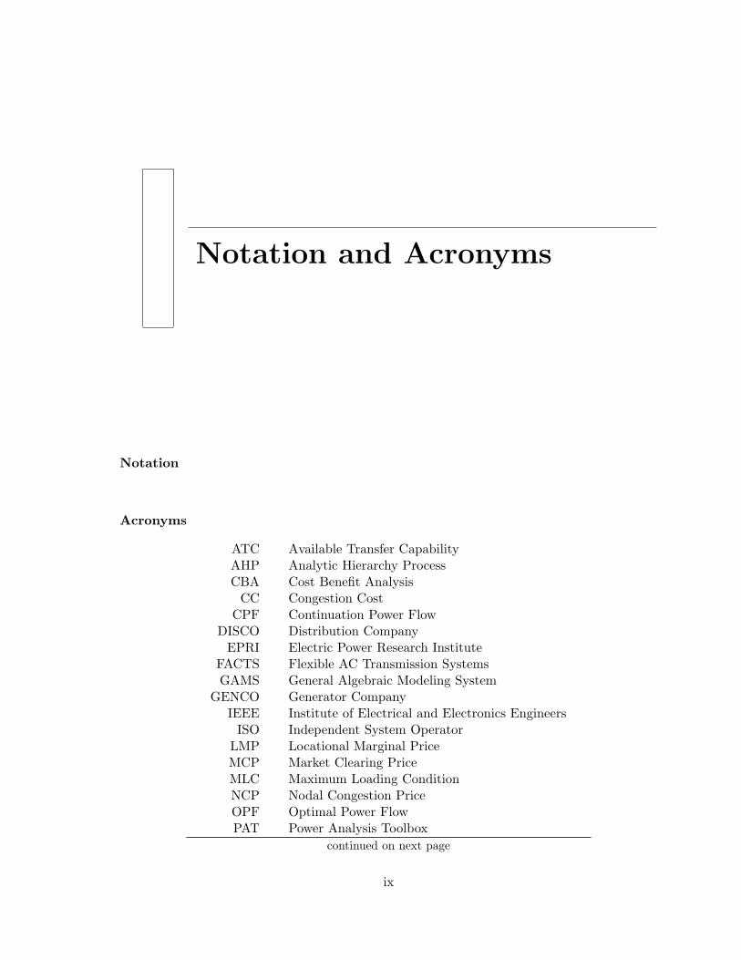
Acronyms
ATC Available Transfer CapabilityAHP Analytic Hierarchy ProcessCBA Cost Benefit Analysis
CC Congestion CostCPF Continuation Power Flow
DISCO Distribution CompanyEPRI Electric Power Research Institute
FACTS Flexible AC Transmission SystemsGAMS General Algebraic Modeling System
GENCO Generator CompanyIEEE Institute of Electrical and Electronics Engineers
ISO Independent System OperatorLMP Locational Marginal PriceMCP Market Clearing PriceMLC Maximum Loading ConditionNCP Nodal Congestion PriceOPF Optimal Power FlowPAT Power Analysis Toolbox
continued on next page
ix

continued from previous pagePF Power Flow
PSAT Power System Analysis ToolboxRMP Reactive Power Marginal PriceSVC Static Var Compensator
TRANSCO Transmission CompanyVAR Volt-Amperes Reactive
VSC-OPF Voltage Stability Constrained Optimal Power Flow
x

Chapter
1
Introduction
1.1 Introduction and Background
During the last two decades, almost all the electric power systems around the world have been
experiencing significant changes due to the privatization and deregulation process. Utilities
are now integrated into decentralized environments in which the planning and operation are
based on the economic principles of open-access markets. In the deregulated environment,
electricity markets are basically competitive and the objective of introducing competition is
to make them more efficient. The basic idea is that if fair and equitable market structures are
established to give all market participants incentives to maximize their own indivual welfare,
then the market as a whole will behave in a manner which maximizes welfare for everyone in
the market [88].
Thus, it is clear that in the competitive market the top most economical aspect is social
welfare where the market suppliers and the consumers supply bids to the market operator.
Consumers should pay the lowest prices for their purchased powers whereas suppliers try
to obtain maximum prices for the supplied energy. The prices should be defined on a fair
basis and the transactions are limited only by the transmission line limits or power exchange
policies. The supply and demand of power should be balanced in real time by dispatching
1

CHAPTER 1. INTRODUCTION 2
the generation in the most economic way possible by respecting all the physical constraints.
The pool or independent system/market operator determines these results by optimizing the
overall system operation. Spot pricing theory based method is most widely used to dispatch
generation and load in the most economic manner.
In competitive markets the primal focus of market and/or system operators is to maintain
system security since the power transactions and the construction of new transmission lines
are inherently associated with it. Transmission congestion occurs when there is insufficient
energy to meet the demands of all customers. System congestion occured due to the thermal
limits on transmission lines or voltage levels may not cause emergency conditions promptly but
should be avoided and therefore by taking this practical consideration, optimization methods
proposed in literature or applied in real time prefers computational efficiency to security
constraints. Voltage collapse have severe and immedeate consequences on system stability and
it is mandatory to avoid congestions associated with it, but voltage collpase issues are rarely
associated with the competitive market studies [19]. Voltage instability may arise following
a trip of a line or a generator, or a combination of eqipment outages. However, an unsually
high load peak or lesser disturbances can cause voltage to fall. If ample reactive power is not
available when voltage falls, reactive reserves are quickly exhausted, and voltage fall further,
possibly collapsing completely.
Voltage Collapse has the following charateristics[62]:
• It is a catastrophic and sudden phenomenon and has typically severe effects on some
network areas and, sometimes, even on the entire grid. Thus precise information about
the proximity to voltage collapse is needed.
• It is generally induced by heavy loading conditions and/or outages which limit the power
transfer capability. Hence the need for N-1 contingency criteria.
• A detailed nonlinear analytical model of power system is required to properly study
voltage collapse phenomena. This is in contrast with the need of computational efficiency
of methods accounting for security and economic dispatch

CHAPTER 1. INTRODUCTION 3
1.1.1 Energy Pricing
In the deregulated power systems, the desired objective to achieve a more efficient power
system is facilitated by competition. In order to achieve proper and efficient competition,
how to establish a good pricing scheme becomes a key issue. Thus it is clear that a simple,
unambiguous and a transparent pricing scheme is required so that the right market signals
can be conveyed to all market pariticipants. Correct price signals will facilitate transmission
access and improve economic efficiency. A good pricing scheme should consist of at least the
following two aspects. First, it should be fair not only to power consumers but also to power
suppliers. In addition, it should he able to stimulate new constructions through providing
proper incentives[47].
Pricing energy on the basis of the location of its withdrawal or injection in a network
proposed in [81] appears to have a universal following in the evolving deregulated electric
power industry. Nodal Pricing is a method of determining prices in which market clearing
prices (MCP) are calculated for a number of locations on the transmission grid called nodes.
Each node represents the physical location on the transmission system where energy is injected
by generators or withdrawn by loads. Price at each node represents the locational value of
energy, which includes the cost of the energy and the cost of delivering it, i.e., losses and
congestion. In all deregulated markets Independent System Operator (ISO) publishes MCP
in real time in the energy market for information purposes, they are often referred to as shadow
prices.
According to PJM: Locatioanal Marginal Price (LMP) or Nodal Marginal Price is the cost
to serve the next MW of load at a specific location, using the lowest production cost of all
available generation, while observing all transmission limits.
The marginal cost to provide energy at a specific location depends on:
• Marginal cost to operate generation
• Total load (demand)
• Cost of delivery on transmission system
• Impact of losses on the interface points

CHAPTER 1. INTRODUCTION 4
1.1.2 FACTS
In the present day scenario,unplanned power transactions are rapidly increasing due to the
competition among utilities to meet the increasing demands and to contracts concluded di-
rectly between producers and consumers. But the power flows should follow the Kirchoff’s
laws and if the transactions are not properly controlled, transmission lines are often operated
and stressed to the limit and beyond the performance capability of their original design and
sometimes overloaded which is termed congestion and thus the full capacity of transmission
interconnections could not be utilized.
Voltage stability, however, is now a major concern in planning and operation electric power
systems. Voltage instability and collapse have resulted in several major system blackouts. One
reason is the need for more intensive use of available transmission facilities. The increased
use of existing transmission is made possible, in part, by reactive power compensation. To
ensure that under these conditions the economical, reliable and secure operation of the grid are
maintained, the need for various aspects of power flow management within the power system
is becoming increasingly evident.
The concept of FACTS and FACTS controllers was first defined by Hingorani in 1988 [43],
[44], [45]. They are high power electronics devices used to control the power flow and enhance
stability, have become, not only common words in the power industry, but they have started
replacing many mechanical control devices. They are certainly playing an important and a
major role in the operation and control of modem power systems. FACTS devices provide
new control facilities, both in steady state power flow and dynamic stability control [35].
These devices have the capability to improve line flows or loadability, contractual requirement
fulfilled, decrease losses, improve voltage profile, increase social benefit, decrease congestion
cost etc, without violating specified power dispatch. Because of their considerable costs it is
important to ascertain the location for placement of these devices.
1.2 Research Motivation and Objectives
Many of today’s power networks are operating close to their stability limits due to economical
reasons; this inturn, has lead to system collapse problems. For heavy loaded systems, when
the operating point approaches the maximum loading point on the P-V curve, the region of

CHAPTER 1. INTRODUCTION 5
attraction is very small; consequently, perturbations cannot be withstanded by the system.
Typically, voltage stability problems are associated with system bifurcations, i.e. saddle-node
or limit induced bifurcations, that lead to voltage collapse [51]. Therefore it is evident that
additional controllers should be added to enhance the overall stability of systems.
Identification of weak buses is an important issue while placing VAR support. An index
to place VAR support based on Cost Benefit Analysis (CBA) is proposed considering social
welfare, congestion cost and maximum loading condition of the system. N-1 contingency
should be considered while chosing the citation for VAR support and the critical line is found
through real power flow sensitivity analysis. To properly include the system security in the
operations of decentralized electricity markets, Voltage Stability Constrained OPF (VSC-
OPF) based market model [62] is chosen for the study with the inclusion of reactive power
production and consumption costs. This multi objective OPF maximizes social welfare and
the distance to maximum loading condition based on the chosen weights. It is demonstrated
that through use of VAR device makes the system more efficient and escalates competition in
the market. The objectives of this work are summarized as follows:
1. Develop an OPF based market model with supply and demand bids for active and also
for reactive powers.
2. Identify weak nodes for the placement of new VAr support, considering both the tech-
nical and economical aspects based on Cost Benefit Analysis (CBA) coupled with N-1
contingency criterion.
3. A method to compute the weights for various parameters of the index which rank optimal
VAr sites.
4. Study the effect of VAr support/SVC on power dispatch and spot prices.
5. Calculate wheeling charges and an analysis of reactive power pricing based on marginal
cost theory.

CHAPTER 1. INTRODUCTION 6
1.3 Outline of the Thesis
This section briefly gives an outline of the remaining chapters of this thesis as follows:
• Chapter 2: Literature Survey
This chapter gives an overview of the research background (Section 2.1) and basics of
electricity markets (Section 2.2) and different entities in it. The literature work on
various indices for optimal placement of VAR support devices in the OPF framework
(Section 2.3) and a brief description of power system analysis toolbox (Section 2.4) are
presented.
• Chapter 3: Standard OPF Model, Pricing and Tools
This chapter presents a brief introduction of OPF based market models (Section 3.1) and
explains in detail about the security constrained OPF (Section 3.2) in the deregulated
electricity market. Transmission pricing (Section 3.3) based on wheeling charges method
and software tools (Section 3.4) used in this thesis and a summary (Section 3.5) are given.
• Chapter 4: Voltage Stability Constrained OPF
The importance of voltage stability (Section 4.1), theory of bifurcation analysis and
methods (Section 4.2) are explained. The modified multi-objective OPF market model,
electricity and nodal congestion pricing details (Section 4.3) coupled with N-1 contin-
gency criterion (Section 4.4) methods based on available transfer capability (ATC) and
a summary (Section 4.5) are presented.
• Chapter 5: VAR Support and Pricing
This chapter explains the necessity of VAR support (Section 5.1), the investment costs
(Section 5.2) associated with it and the index for optimal placement of FACTS (Section
5.3) devices. The concept of VAR pricing based on marginal theory and effect of load
power factor on reactive power marginal prices (Section 5.3.4) with a brief summary
(Section 5.5) are discussed.
• Chapter 6: System Studies
The test systems description (Section 6.1), results and discussions for 6-bus (Section
6.2), IEEE 14-bus (Section 6.3) are summarized (Section 6.4).
• Chapter 7: Conclusions an Future Work

CHAPTER 1. INTRODUCTION 7
This chapter presents principal contributions (Section 7.1) and possible future directions
(Section 7.2).
In Appendix A.1 the network and market data of the 6-bus (A.1.2) and IEEE 14-bus
(A.1.3) are given.

Chapter
2
Literature Review
2.1 Introduction
Deregulation is defined as the process by which governments remove restrictions on business
and individuals in order to (in theory) encourage the efficient operation of markets. Due to
the recent transition from government controlled to deregulated electricity markets, the rela-
tionship between power system controllers and electricity markets has added a new dimension,
as the effect of these controllers on the overall power system stability has to be seen from an
economic point of view [50]. Transmission systems are being required to provide increased
power transfer capability and to accommodate a much wider range of possible generation
patterns. Environmental, right-of-way, and cost problems are major hurdles for power trans-
mission network expansion. Hence, there is an interest in better utilization of available power
system capacities by installing new devices such as FACTS.
This thesis mainly focuses on the voltage stability constrained optimal power flow ap-
proach to properly include security constraints in the competitive electricity markets. The
effect of VAR support such as FACTS device/SVC on power dispatch and electricity market
prices is the main concern. Transmission pricing is an important issue in view of increased
deregulation. FACTS devices had the ability to reduce the overall operating cost and their
8

CHAPTER 2. LITERATURE REVIEW 9
Figure 2.1: Supply and Demand Curve [98]
impact on transmission pricing. A detailed literature survey on various techniques used for
finding optimal location for the placement of VAR support and effect of load power factor on
reactive power marginal prices is presented in the following sections.
2.2 Electricity Markets Introduction
Market is a place where buyers and sellers meet to exchange goods and services. An electricity
market is a system for effecting the purchase and sale of electricity using supply and demand
to set the price. The theory of supply and demand describes how prices vary as a result of
a balance between product availability at each price (supply) and the desires of those with
purchasing power at each price (demand). The graph 2.1 depicts an increase in demand from
D1 to D2 along with the consequent increase in price and quantity required to reach a new
market-clearing equilibrium point on the supply curve (S). The slope of the demand curve
(downward to the right) indicates that a greater quantity will be demanded when the price is

CHAPTER 2. LITERATURE REVIEW 10
lower. On the other hand, the slope of the supply curve (upward to the right) tells us that
as the price goes up, producers are willing to produce more goods. The point at which these
curves intersect is the equilibrium point.
Electricity is by its nature difficult to store and the supply and demand has to be balanced
in realtime. Unlike other products, it is not possible, under normal operating conditions, to
keep it in stock. Demand and supply vary continuously. In the past, the electric power industry
has been vertically integrated, meaning that a central authority monitored and controlled
all the activities in generation, transmission, and distribution. For the last decade or so,
the electric power industry has been undergoing a process of transition and restructuring,
in particular the separation of transmission from generation activities. There is therefore a
physical requirement for a controlling agency, the power system operator, to coordinate the
dispatch of generating units to meet the expected demand of the system across the transmission
grid. This system operator must never be involved in the market competition, and is usually
called the Independent System Operator (ISO)
2.2.1 Various Entities in Deregulated Electricity Market
Many new entities were introduced in the new restructured market. The usual separation of
the electric power industry distinguishes among generation, transmission and distribution.
Generation Companies: GENCOs
Operates and maintains existing generating plants. The Gencos interact with the short term
market acting on behalf of the plant owners to bid into the short-term power pool for economic
dispatch. There are many participants with existing plants and no barriers to entry for
construction of new plants.
Transmission Companies: TRANSCOs
This segment is regulated to provide open access, comparable service and cost recovery. Con-
structs and maintains the network of transmission wires. This entity should ensure the avail-
ability of the transmission system to all the entities in the system.
Distribution Companies: DISCOs
They own and operate local distribution companies. This entity purchases electricity in the

CHAPTER 2. LITERATURE REVIEW 11
wholesale market and supply it to the final customers.
Energy Services Companies: ESCOs
These may be large industrial customers, customer pools or private companies, and their
main goal is to purchase power at the least cost for their customers from GENCOs. They
participate in the market like DISCOs, except that they do not own or operate the local
distribution companies.
Customers
These are the consumers of electricity. Depending on the market structure, the customers
have various options for purchasing electricity. They can choose to purchase electricity from
the spot-market by bidding for purchase, or buy directly from a GENCO, a DISCO or an
ESCO.
Independent System Operator: ISO
An entity that will monitor the reliability of the power system and coordinate the supply
of electricity around the state. ISO is a non-profit corporation that uses governance models
developed by the Federal Energy Regulatory Commission. In the electricity market dereg-
ulation it also acts as a marketplace in wholesale power. Regional Transmission Operators
(RTOs) such as the Pennsylvania-New Jersey-Maryland Interconnection (PJM) have the same
function and responsibility but operate within more than one U.S. state.
2.2.2 Market Clearing Mechanism
In most markets, both GENCOs and ESCOs bid in the market. A market clearing price (MCP)
is obtained, as illustrated in Figure 2.2, by stacking the supply bids in order of increasing
prices and the demand bids in order of decreasing prices. The MCP and the amount of energy
cleared for trading are obtained from the intersecting point of these curves. This market
clearing process is referred to as double-sided auction power pools [85].
However, the load in most markets does not actively bid, i.e. the load is inelastic. In this
case, the system price is cleared by matching the supply curve with a forecast of undispatchable
load. Typically, only GENCOs submit bids that are stacked in increasing order of prices, The
highest priced bid to intersect with the system demand forecast determines the MCP and such

CHAPTER 2. LITERATURE REVIEW 12
Figure 2.2: Double-sided auction markets
CHAPTER 2. LITERATURE REVIEW 13
a market model is known as a single or one-sided auction power pool.
Double-sided auctions are a better setting for thinking about price formation than one-
sided auctions, both because they are often a better match to reality, and especially because
they capture the essential problems of trade better than one-sided auctions. In this thesis, we
use double-sided auctions.
UK Power Market [93]:
UK was one of the first nations to embark upon widespread privatization of its power
industry. In 1987 fall, UK authority started to privatize its electric utilities, and separate
generation, transmission and distribution sectors. The Electricity Pool of England and Wales
has been in operation since 1990, where competition was only introduced into generation
sector. In the beginning, UK power market was a “single buyer” which bought all electricity
from generation companies through a spot market, and then sold directly to customers at an
uniform system price. UK pool is a single commodity market where only energy is traded,
and virtually all energy transactions must go through the pool.
As a means of controlling price volatility, a hedging market called “contract for differ-
ences” (CFD) market allows for bilateral contracts to be negotiated between generators and
consumers. However, CFD are purely financial contracts without exposition to public. Re-
cently UK power market has undergone a significant reform. A series of markets: a futures
market, a short-run bilateral market and so on, have been setup in order to enhance compe-
tition in local distribution, simplify pricing mechanism and strengthen market transparency
and liquidity.
California Power Market [14]:
In December, 1995, the California Utility Commission (CPUC) issued its policy on electric
industry restructuring to replace administrative regulation with competitive market forces,
and AB 1890 was signed in 1996, which called for the deregulation of Californias investor
owned electric utilities (IOUS). The law established an Oversight Board, an Independent
System Operator (IS0), and a Power Exchange (PX). On April 1, 1998, the power industry
in California began a phased-in process of deregulation.
The ISO controls power dispatch and transmission system, but it owns no transmission,
generation, or distribution facilities and has no financial interest in the PX, or in any generation

CHAPTER 2. LITERATURE REVIEW 14
or load. The ISO also manages transmission congestion, procures ancillary service through a
market.
The PX is mandatory for utility generation and procurement by the IOUS, but voluntary
for all other market participants. The PX is an independent entity that provides a forward
competitive spot market for electric power, conducts day-ahead and hour-ahead auctions of
generation and demand, ensures non-discriminatory, transparent bidding interface and pro-
tocols. The PX also develops balanced generation and load schedules for transmittal to the
IS0.
California power market is a “wholesale” market, and allows flow based bilateral trans-
actions to coexist with the PX spot market. Bilateral contracts and the voluntary PX are
operated in parallel.
Nordic Power Market [69]
The Norwegian market was effectively deregulated in 1991, with Sweden joining as a
full-fledged member in 1996, Finland in 1998, and Denmark recently. These three countries
constitute one closely integrated power market where power is traded via bilateral contracts
and on a common spot market exchange (Nerd Pool). The system operator in each county is
respectively in charge of its system security and coordinate cross-country trading with each
other. The Nordic power market is a “retail competition” market where end-customers have
full freedom to select power suppliers.
The Nordic power market is mainly based on bilateral contracts, and generation reserve
is not much of a problem because the system is predominantly hydro. In addition, besides a
spot market, two financial markets: futures market (Eltermin) and options market (Elopticm)
were developed for price hedging and risk management.
PJM Power Market [76]
PJM’s markets are “wholesale markets” involving only purchase and sale of power for
resale. All buyers, sellers, transmission users and transmission owners within the PJM control
region must be members of PJM. Sellers and buyers located outside of PJM may buy and sell
power into and out of PJM, are not required to be members, but must obtain transmission
service under different tariffs. Sellers may choose to self supply, sell into PJM auction markets
or privately through bilateral contracts with buyers. Buyers may choose to self supply, buy
CHAPTER 2. LITERATURE REVIEW 15
from PJM auction markets or through bilateral contracts with sellers (either generators or
resellers of generation). End users do not participate directly and are served by resellers.
It consists of Energy Markets (Day ahead, real time (balancing) markets), Ancillary Ser-
vices, Unforced Capacity Obligation (UCAP). Energy, Ancillary Services and UCAP may be
bought at auction, bilaterally or self supplied. PJM constantly calculates the least cost gen-
eration mix solution to serve instantaneous load, constrained by system security limits. PJM
redispatches generation, as necessary, to serve load. Generation is paid its bus price (bid based
price, not cost based). Load pays for MW consumed at its bus, plus the difference between
source and sink prices.
Day Ahead Market - Sellers and Buyers bid into each hour of the 24 hour day ahead period
bids are stacked for each hour lowest marginal price which supplies all demand sets LMP for
that hour.
Real Time Market Uncommitted Buyers and Sellers may self schedule (accept real time
price), but successful day ahead bidders must honor their bids or cover from spot market at
their own expense.
2.3 Optimal Power Flow
In view of deregulation, it is important for the independent system operator to operate power
system in a more reliable and economical way. This involves a lot of decision making process
and the softwares used to simulate and analyze the electricity market behavior are mostly
based on OPF algorithms. The optimal power flow (OPF) is an important software in the
energy management system (EMS). OPF was born in 1962 [22] and took a long time to become
a successful algorithm that could be applied in every days use. The OPF-based approach is
basically a nonlinear constrained optimization problem, and consists of a scalar objective
function and a set of equality and inequality constraints [3], [66], [91]. The objective function
varies from one system operator to another and also with the necessity. In [48] the autors
classified the optimal power flow methods based on the choice of optimization techniques.
The security constrained optimal power flow [59] implemented by many researchers is to
minimize the cost of generation or dispatch while satisfying set of constraints such as power
flow equations, active and reactive power bounds on generators, voltages at all nodes and
thermal/active power limits on transmission lines.

CHAPTER 2. LITERATURE REVIEW 16
Non-linear optimization techniques are shown to be adequate for maximization of the
loading parameter in voltage collapse studies as discussed in [16], [18], [19], [49], [80], [99]. In
this thesis a modified multi-objective approach [61] is chosen to properly represent security
in on-line market computations so that social welfare and the distance to collapse point are
maximized at the same time. The problem is formulated as a mixed integer non-linear pro-
gramming (MINLP) and is solved using General Algebraic Modeling System (GAMS) [12].
In this thesis contingencies are included using methods based on what proposed in [63] and
further extended to a multi-objective optimization as cited in [61].
Optimal power flow based models are widely used for market solutions because the dual
variables associated with power flow constraints gives the shadow prices which are then used
in spot pricing [31] with least computational effort. Spot pricing was originally defined for
active power transactions, considering only congestion alleviations [78], [81] and then extended
to account for different price components, such as reactive pricing and ancillary services [10],
[32]. In [41] authors detail the use of the reactive power services and demonstrate that the
reactive power production costs should be included in the formulations for the calculation of
the reactive power cost prices. A formulation for the reactive power production cost calculation
is proposed by Lamont and FU [54] and the concept of opportunity cost is introduced. In this
work for the sake of simplicity the cost of producing reactive power from generators is taken
as percentage of real power generation cost without losing any generality. The active power
dispatch minimizes losses as long as the system is not congested. However if the transmission
system is congested losses are not equally distributed among the generators.
Some of the objectives of the OPF are:
• Minimize system real & reactive power losses
• Minimize generation fuel costs
• Optimize power exchange with other systems (on-site generation, utilities, IPP’s, &
power grids)
• Control generator’s MW (governor) & MVAR (AVR) settings within the specified limits
• Maximize voltage & flow security indices
• Minimize load shedding

CHAPTER 2. LITERATURE REVIEW 17
• Maximize Social Welfare
• Minimize generator fuel cost or heat rate with different cost models & fuel profiles
2.3.1 OPF with VAR Support Devices
The possibility of operating the power system at the minimal cost while satisfying specified
transmission constraints and security constraints is one of main current issues in stretching
transmission capacity by the use of controllable FACTS. The conventional OPF program
must undergo some changes such as inclusion of new control variables belonging to FACTS
devices and the corresponding load flow solutions to deal with the above said problem. In
[40] presented a review literature, which addresses the application of FACTS, concepts for the
improvement of power system utilization and performance.
The four typical FACTS devices that are used in general with OPF are Static Var Com-
pensator (SVC) [5], [17], [37], [46], [74] Thyristor Controlled Series Capacitor (TCSC) [17],
[33], [46], Thyristor Controlled Phase Angle Regulator (TCPAR) [34], [71], [79] , Unified Power
Flow Controller (UPFC) [6], [7], [23], [38], [42], [70], [74]. The reactance of the line can be
changed by TCSC . TCPAR varies the phase angle between the two terminal voltages and
SVC can be used to control the reactive compensation. The UPFC is the most powerful and
versatile FACTS device due to the fact that the line impedance, terminal voltages, and the
voltage angle can be controlled by one and the same device.
The power flow Pij through the transmission line i− j is a function of the line reactance
Xij , the voltage magnitude Vi, Vj and the phase angle between the sending and recieving end
voltages δi − δj as shown in equation 2.1.
Pij =ViVj
Xijsin(δi − δj) (2.1)
The above-mentioned FACTS devices can be used to control the power flow by changing the
transmission line parameters so that the power flow can be optimized. The reactive power
compensation of AC transmission systems using fixed series or shunt capacitors can solve
some of the above associated problems with AC networks. However the slow nature of control
using mechanical switches (circuit breaker) and limits on the frequency of switching imply
that faster dynamic controls are required to overcome the above mentioned problems [1].

CHAPTER 2. LITERATURE REVIEW 18
Several algorithms have been proposed in literature to solve power flow and optimal power
with different FACTS devices. New control variables and control objective equations are
usually added in conventional power flow equations. Singinificant number of efforts have been
made to study the impact of FACTS on electricity prices. The purpose of pricing is to recover
cost of transmission and to encourage efficient use and investment. OPF based spot pricing
is an important method. In [27] Choi presented theory and simulation results of real time
pricing of real and reactive powers that maximizes social benefit. In [72], authors have shown
the ability of FACTS devices to change the production cost and their impact on transmission
charges. FACTS devices had the ability to reduce the overall operating cost and their impact
on transmission pricing. In [90] SVC and TCSC are considered to show the above mentioned
benefits of FACTS. But the optimal placement of FACTS is found through trial and error
method. Most of the literature [11], [29], [56], [74], [86] are either based on minimum price
dispatch algorithm or maximum social welfare [88], [89], [90], [95]. Optimization has been
performed with the system operating constraints.
These market models consider the offline power flow limits and the security is simply repre-
sented by voltage limits which gives higher congestion prices and spot prices are heterogeneous
[61], [65]. To properly include the security costs in the market prices the multi-objective op-
timal power flow which maximized both social welfare and loadability point is considered in
this research. To best utilize the benefits of sources, optimal allocation of FACTS should be
performed. A brief literature suvey on optimal locatin is presented in the following section.
2.3.2 Location of VAR Support
Congestion in a transmission system, whether vertically organized or unbundled, cannot be
permitted except for a very short duration, for fear of cascade outages with uncontrolled loss
of load. The role of FACTS in the open power market is to manage the congestion, enhancing
security, reliability, increasing loadability or available capability, controlled flow of power, and
other system performances. It is important to ascertain the location of these devices because
of their significant costs.
Optimal placement of FACTS using Genetic Algorithms (GA’s) is implemented in [55],
[73], [75]. In [36], authors used system loadability as the index but they didnot consider the
cost of FACTS devices and their impact on generation profile. Optimal location considering

CHAPTER 2. LITERATURE REVIEW 19
the generation cost of the power plants and investment cost of the devices is employed in
[13] to evaluate the power system performance. The location of FACTS devices for reactive
compensation is performed according to reactive marginal cost criterion in [74]. In [57], [72]
the optimal location of FACTS devices are obtained by solving the economic dispatch problem
plus the cost of these devices making the assumption that all lines initially have these devices.
In [89] the optimal placement of a prefixed amount of FACTS devices is developed in an
electricity market having pool and contractual dispatches by a two-step procedure. First, by
using a sensitivity-based approach the few locations of FACTS devices is decided and then
the optimal dispatch problem is solved to select the optimal location and parameter settings.
In [67] a parallel tabu search based method, for determining the optimal allocation of UPFC
devices is proposed.
Location of TCSC is taken as the best when it achieves the maximum social benefit in
[88] and used a real power flow sensitivity as an index in [95]. In [21] SVC is placed where it
improves the maximum loadability of the system as well as the voltage profiles at the most
remote load buses. In [53], VAR support at the pilot bus improves overall system voltage
profile and loading margin. The authors considered N-1 criterion but they didnot consider
various costs associated with the generation. Chattopadhyay et al presented [24] an integral
framework for optimal reactive power planning and its spot pricing in which the selection of
VAR source sites is based only on the real power generation operation benefit-to cost ratio for
a capacitor on load node. The authors considered the cost of VAR support in the objective and
the approach is superior to traditional heuristic methods in which the location of new VAR
devices are either simply estimated or directly assumed. However, it neglects the benefits of
decrease in congestion cost and increase in system loadability in the selection of weak buses.
In this thesis, a multi-objective market model [61] that maximizes the social welfare as
well as distance to collapse point is adopted. The influence of any of these terms on market
prices can be studied by adjusting the corresponding weight allocated to it. A new index
which considers the social welfare, congestion cost and maximum loadability coupled with N-
1 contingency criterion for identifying the weak candidate buses based on Cost Benefit Analysis
(CBA) is proposed in this thesis. All BCRs reflect the improvement of the systems operation
state after the VAR support service is provided. The relative weights for each parameter
are computed using analytic hierarchical process(AHP). The index and the methodology are

CHAPTER 2. LITERATURE REVIEW 20
explained in section 5.3.
2.4 Power System Analysis Toolbox (PSAT)
The power system analysis toolbox (PSAT) [77] is a MATLAB based toolbox for static and
dynamic analysis of electric power systems. PSAT includes power flow, continuation power
flow, optimal power flow, small signal stability analysis and time domain simulation. All
functions can be accessed by means of graphical user interfaces (GUIs) and a Simulink-based
library which provides an user friendly tool for network design.
Package PF CPF OPF SSSA TDS GUIEST [96]
√ √ √
MatEMTP [60]√ √
Matpower [100]√ √
PAT [82]√ √ √ √
PSAT [77]√ √ √ √ √ √
PST [28]√ √ √
SPS [92]√ √ √ √
VST [26]√ √ √ √ √
Table 2.1: Comparison of MATLAB-based packages for power system analysis[77]
Table (2.1) depicts a brief comparison of the existing MATLAB-based packages for power
system analysis. The features illustrated in the table are power flow (PF), continuation power
flow (CPF), optimal power flow (OPF), small signal stability analysis (SSSA), time domain
simulation (TDS) along with features such as graphical user interface (GUI).
Chapter
3
Standard OPF Model, Pricingand Tools
3.1 Introduction
A concept of electricity energy market, which reflects the generation cost on the price of
electricity, is suggested to replace conventional load management strategy. This market takes
charge of transmission and distribution of electricity and decides the price of electricity so as to
balance the demand and supply of electricity. Participants participate in this market by selling
and buying electricity. Electricity auction problem can be solved by two approaches, merit
order or single-price auctions and OPF-based power markets. Though the market clearing
mechanisms applied by different competitive pool-based electricity markets significantly varies,
there are some common characteristics. The main drawback of the first approach is, there
is a need of separate procedure to take into account congestions and in general, non linear
constraints. Therefore we will concentrate only on OPF based hybrid markets. As a matter of
fact, OPF methods have been used in regulated power systems to schedule power generations in
order to minimize cost productions and losses in transmission lines. OPF main characteristics
are as follows:
• Precise power system models can be represented in OPF by including variety of (non-
21

CHAPTER 3. STANDARD OPF MODEL, PRICING AND TOOLS 22
linear) constraints.
• Having complex and unclear solution process OPF is not very popular among market
operators.
• System losses and transmission congestions are taken into consideration without any
additional procedures.
• The existing solvers for Nonlinear Programming and Mixed Integer Nonlinear Program-
ming are less efficient which is a critical issue for on-line applications.
The OPF based approach to maximize the social welfare is explained in the next section.
3.2 Security Constrained OPF Market Model
The objective of pricing policy is to maximize the benefit of all the participants, that is, to
maximize the consumers and producers surplus, subject to operational constraints. This is
accomplished by setting the prices of real and reactive powers at each bus at a particular
time equal to the marginal values of supplying and consuming real and reactive power at the
same bus and at the same time, where the marginal values are determined by maximizing total
surplus of utilities and consumers, subject to the operational constraints. The social welfare in
equation 3.2 ensures that generators get the maximum income for their power production and
consumers or wholesale retailers pay the cheapest prices for their power purchase as follows:
Max. Sw =∑j∈J
BPj (PDj ) + BQj (QDj ) −∑i∈I
CPi(PSi)− CQi(QGi) (3.1)
QDj = PDj tan(φDi)
where
I is set of pool supplier buses;
J is set of pool load buses;
PSi is active power of pool supplier-i;
QGi is reactive power of pool generator-i;
CPi is real power bid price of pool supplier-i in $/MWh;
CQi is reative power bid price of pool generator-i in $/MV Arh;

CHAPTER 3. STANDARD OPF MODEL, PRICING AND TOOLS 23
PDj is active power of pool load-j;
QDj is reactive power of pool load-j;
BPj is real power bid price of pool load-j in $/MWh;
BQj is reactive power bid price of pool load-j in $/MV Arh;
The objective function of this OPF is to maximize the net social welfare which is the
difference between the total consumer benefit and cost of generation.
The operating constraints are as follows:
1) Equality Constraints:
Power flow equations corresponding to both real and reactive power balance equations are the
equality constraints that can be written, for all the buses.
Ph = V 2h (gh + gh0)− Vh
nl∑l 6=h
Vl(ghl cos(θh − θl) + bhl sin(θh − θl)) ∀h ∈ B (3.2)
Qh = −V 2h (bh + bh0) + Vh
nl∑l 6=h
Vl(ghl sin(θh − θl)− bhl cos(θh − θl)) ∀h ∈ B
where Ph and Qh are the real and reactive powers injected at bus h, Vh and θh are the voltages
and phasor angles at bus h, B is the set of indexes for network buses, nl is the number of
connections departing from bus h and gh, gh0, bh, bh0, ghl and bhl are line parameters, namely
conductances and succeptances, as commonly defined in literature.
In the following, power injections are modeled as the sum of generator and load powers con-
nected to the bus h, as follows:
Ph =∑i∈Ih
(PGi0 + PSi)−∑j∈Jh
(PL0j + PDj ) ∀h ∈ B (3.3)
Qh =∑i∈Ih
QGi −∑j∈Jh
(PL0j + PDj ) tan(φDi) ∀h ∈ B
QL = PLtan(φL) (3.4)
where Ih and Jh are the sub-sets of generators and loads connected to bus h, respectively.
PG0 and PL0 are fixed power amount defining the base case condition and PS and PD are
variable powers, which will be called power supply and power demand bids respectively. In all

CHAPTER 3. STANDARD OPF MODEL, PRICING AND TOOLS 24
test cases used in this thesis, load reactive powers are assumed to be dependent on the real
powers by a constant power factor φL, thus leading to:
y∆= f(x, p) = f(V, θ, PG, QG, PL, QL) (3.5)
where x is a vector of dependent variables and p is a vector of independent or control variables.
In a standard single slack bus power flow formulation, dependent variables are voltage magni-
tudes V and phases θ at the load buses, generator reactive powers QG and voltage phases at
the generator buses, while control variables are generator active powers PG, load powers PL
and QL and the slack bus voltage. In distributed slack bus voltage models, y includes also an
additional variable, say kG, which forces all generators to share losses [9].
PG = (1 + kG)(PG0 + Ps) (3.6)
Equations 3.3 are for single slack bus model, and do not include slack bus real power which is
actually a dependent variable, while for the distributed slack bus model where as equation 3.6
is valid for all generators, including the reference phase angle generator.The distributed slack
bus model will be used in this thesis in OPF problems since it allows a fair and reasonable
distribution of transmission losses among all market suppliers. Firstly the active and reactive
power balance is ensured, then transmission losses are accurately modeled and taken into
account.
2) Inequality Constraints:
1. Supply Bid Blocks:
PSmini≤ PSi ≤ PSmaxi
∀i ∈ I (3.7)
where PSminiand PSmaxi
are the minimum and maximum bids of real power offered by
unit i, respectively and I is the set of indexes of generating units.
2. Demand Bid Blocks:
PDminj≤ PDj ≤ PDmaxj
∀j ∈ J (3.8)
where PDminjand PDmaxj
are the minimum and maximum bids of real power demanded
by consumer j, respectively and J is the set of indexes of consumers.

CHAPTER 3. STANDARD OPF MODEL, PRICING AND TOOLS 25
3. Generator Reactive Power Support :
QGmini≤ QGi ≤ QGmaxi
∀i ∈ I (3.9)
where QGminiand QGmaxi
are the minimum and maximum limits of the reactive power
support available at unit i, respectively and I is the set of indexes of generating units.
4. Voltage “Security” Limits:
Vminh≤ Vh ≤ Vmaxh
∀h ∈ B (3.10)
where Vminhand Vmaxh
are the minimum and maximum allowed voltage magnitues at
bus h, respectively and B is the set of indexes of network buses.
5. Thermal Limits:
Ihk(θ, V ) ≤ Ihkmax ∀(h, k) ∈ N (3.11)
Ikh(θ, V ) ≤ Ikhmax
where Ihk and Ikh are the line currents and are used to model system security by limiting
transmission line flows, respectively and N is the set of indexes of transmission lines. All
electric lines produce heat and therefore have a limit on the amount of power they can
carry to prevent overheating. The actual temperatures occurring in the transmission
line equipment depend on the current, that is the rate of flow of the electrons, and also
on ambient weather conditions, such as temperature, wind speed, and wind direction,
because the weather effects the dissipation of the heat into the air.
The thermal ratings for transmission lines, however, are usually expressed in terms of
current flows, rather than actual temperatures for ease of measurement. A “normal”
thermal rating for a line is the current flow level it can support indefinitely. Emergency
ratings are levels the line can support for specific periods, for example, several hours.
6. Power Limits:
In common practice [97], the inclusion of system congestions in the OPF problem is ob-
tained by imposing transmission capacity constraints on the real power flows, as follows:
|Phk(θ, V )| ≤ Phkmax ∀(h, k) ∈ N (3.12)
|Pkh(θ, V )| ≤ Pkhmax
CHAPTER 3. STANDARD OPF MODEL, PRICING AND TOOLS 26
where Phk and Pkh are obtained by means of off-line angle and/or voltage stability studies.
Hence, these limits do not actually represent the actual stability conditions of the resulting
OPF problem solution, which may lead in some cases to insecure solutions and/or inadequate
price signals, as demonstrated in [62].
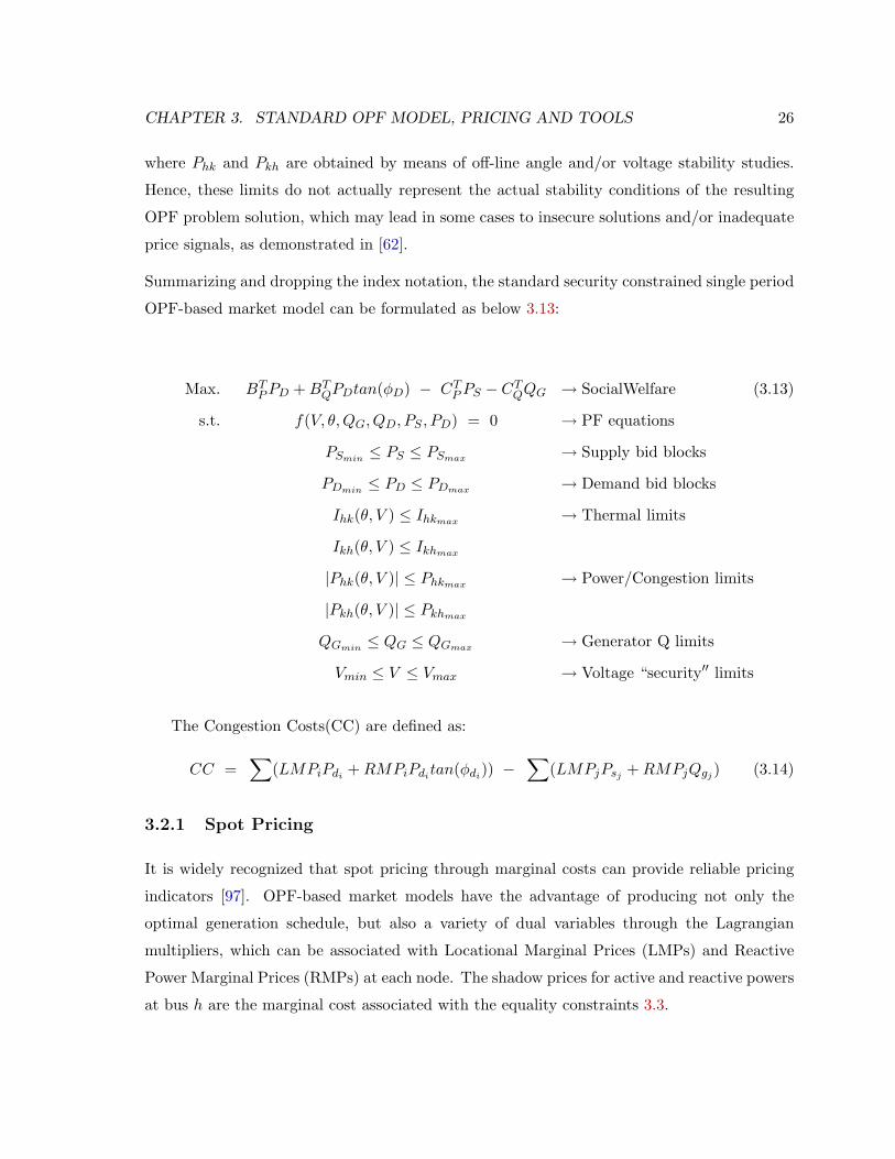
Summarizing and dropping the index notation, the standard security constrained single period
OPF-based market model can be formulated as below 3.13:
Max. BTP PD + BT
QPDtan(φD) − CTP PS − CT
QQG → SocialWelfare (3.13)
s.t. f(V, θ,QG, QD, PS , PD) = 0 → PF equations
PSmin ≤ PS ≤ PSmax → Supply bid blocks
PDmin ≤ PD ≤ PDmax → Demand bid blocks
Ihk(θ, V ) ≤ Ihkmax → Thermal limits
Ikh(θ, V ) ≤ Ikhmax
|Phk(θ, V )| ≤ Phkmax → Power/Congestion limits
|Pkh(θ, V )| ≤ Pkhmax
QGmin ≤ QG ≤ QGmax → Generator Q limits
Vmin ≤ V ≤ Vmax → Voltage “security′′ limits
The Congestion Costs(CC) are defined as:
CC =∑
(LMPiPdi+ RMPiPdi
tan(φdi)) −
∑(LMPjPsj + RMPjQgj ) (3.14)
3.2.1 Spot Pricing
It is widely recognized that spot pricing through marginal costs can provide reliable pricing
indicators [97]. OPF-based market models have the advantage of producing not only the
optimal generation schedule, but also a variety of dual variables through the Lagrangian
multipliers, which can be associated with Locational Marginal Prices (LMPs) and Reactive
Power Marginal Prices (RMPs) at each node. The shadow prices for active and reactive powers
at bus h are the marginal cost associated with the equality constraints 3.3.

CHAPTER 3. STANDARD OPF MODEL, PRICING AND TOOLS 27
The Lagrangian function for 3.13 is as follows :
Min. L = Sw − ρT f(θ, V,QG, QD, PS , PD) (3.15)
− µTPSmax
(PSmax − PS)
− µTPSmin
(PS − PSmin)
− µTPDmax
(PDmax − PD)
− µTPDmin
(PD − PDmin)
− µTIhkmax
(Imax − Ihk)
− µTIkhmax
(Imax − Ikh)
− µTPhkmax
(Pmax − Phk)
− µTPkhmax
(Pmax − Pkh)
− µTQGmax
(QGmax −QG)
− µTQGmin
(QG −QGmin)
− µTVmax
(Vmax − V )
− µTVmin
(V − Vmin)
At a particular instant, real time price of real power and reactive power at bus-h can be
given by 3.16, A more detailed information can be deduced from the KKT optimality condition
LMPh =∂L
∂Ph= ρPh
(3.16)
RMPh =∂L
∂Qh= ρQh
applied to the OPF problem.
3.2.2 Nodal Congestion Pricing
Using the decomposition formula proposed in [97] for LMPs one can define a vector of active
and reactive Nodal Congestion Prices (NCPs) as follows:
NCP =(
∂fT
∂x
)−1∂HT
∂x(µmax − µmin) (3.17)
where x = (θ, V ) are voltage phases and magnitudes, H represents the inequality constraint
functions (e.g. transmission line powers and currents), and µmax and µmin are the dual

CHAPTER 3. STANDARD OPF MODEL, PRICING AND TOOLS 28
variables or shadow prices associated to inequality constraints.
Equation (3.17) for the standard security constrained OPF (3.13) becomes:
NCP = [Dxf ]−1
∂Ihk
∂x(µIhkmax
− µIhkmin) +
∂Phk
∂x(µPhkmax
− µPhkmin) +
0
µVmax − µVmin
(3.18)
NCP for real power injection h can be conveniently written as:
NCPh =lk∑
k=1
(µIhkmax− µIhkmin
)∂Ihk
∂Ph(3.19)
+lk∑
k=1
(µPhkmax− µPhkmin
)∂Phk
∂Ph
where lk is the number of lines departing from bus h. Observe that in (3.18) dual variables
or shadow prices µPhkmaxand µPhkmin
directly affect NCPs, which is the main drawback of
transmission congestion limits Phkmax computed off-line.
3.3 Transmission Pricing
The transmission of electricity differs from transportation of any typical commodity by some
inherent aspects such as; production needs to match the consumption at the same time; system
control is not an easy task; the electricity flows donot usually follow the economic law. The last
aspect is normally observed when transmission systems are included in an economic dispatch
problem. Transmission is therefore the main concern in the establishment of real competition
in the electricity market.
Transmission pricing has been an important issue on the ongoing debate about power
system restructuring and deregulation. The purpose of pricing is to recover cost of transmission
and to encourage efficient use and investment. The effect of FACTS devices on transmission
charge varies according to the pricing methodology adopted. FACTS devices had the ability to
reduce the overall operating cost and their impact on transmission pricing. Impact of FACTS
on wheeling charges is being addressed in this thesis. This is becoming an important issue
when transmission open access schemes are introduced. Investments on both transmission and
generation sides are really changed by these charges.

CHAPTER 3. STANDARD OPF MODEL, PRICING AND TOOLS 29
Pricing methods based on incremental cost and embedded cost methods [87] can be used
to assess the impact of FACTS devices on transmission charges. The incremental cost methods
are based on the variation of system total costs when a wheeling transaction is accomodated.
The marginal cost is an example of this technique. This method is adopted in this thesis.
3.3.1 Wheeling Charges Method
According to economic theory, pricing transmission service by marginal cost is most acceptable.
If MCpB and MCqB are the marginal costs of real and reactive powers at a buyer bus while
MCpS and MCqS are at a seller bus, wheeling rate for real power is given by,
Wp = MCpB − MCpS (3.20)
Similarly wheeling rate for reactive power is given by,
Wq = MCqB − MCqS (3.21)
Total wheeling charges for the purchase of real power (PB) and reactive power (QB) are
given as,
WCp = PB ×Wp (3.22)
WCq = QB ×Wq (3.23)
3.4 Software Tools
The electricity market structure with both supply and demand side bidding is considered in
the OPF framework. It is assumed that each generation bus or GENCO and load bus or ESCO
supply their bids to the operator in $/MWh. The maket bids and limitations of transmission
lines and restrictions on voltage limits and maximum power output of different sources are
forumulated in a OPF structure. The problem is formulated as a Mixed Integer Nonlinear
Programming and is solved by General Algebraic Modeling Systems (GAMS).
3.4.1 PSAT-GAMS
In the field of general purpose optimization techniques, one of researcher’s favourite choice
is the General Algebraic Modeling Systems (GAMS). GAMS is a highlevel modeling system

CHAPTER 3. STANDARD OPF MODEL, PRICING AND TOOLS 30
Figure 3.1: Structure of the PSAT-GAMS interface [62]
for mathematical programming problems. It consists of a language compiler and a variety
of integrated high-performance solvers. GAMS is specifically designed for large and complex
scale problems, and allows creating and maintaining models for a wide variety of applications
and disciplines [12]. GAMS is able to formulate models in many different types of problem
classes, such as linear programming (LP), nonlinear programming (NLP), mixed-integer linear
programming (MILP) and mixed-integer nonlinear programming (MINLP).
The existing PSAT-GAMS interface has been used to solve the market problem. Before
the interface can be used, one has to create data file describing the system. At this aim the
user can use the PSAT-Simulink interface and draw the on-line diagram of the network or load
a predefined test network which is provided within the PSAT main distribution. The second
step is solving the power flow. At this point, the PSAT-GAMS interface can be opened and
CHAPTER 3. STANDARD OPF MODEL, PRICING AND TOOLS 31
the GAMS solvers launched. Observe in figure 3.1 that only networks for which market data
have been defined can be used with the PSAT-GAMS interface. If no market data has been
defined, the interface simply terminates with a warning message. A command line version of
PSAT is also provided to make it feasible to use it inside the matlab applications.
The interface works as follows: the system information are “translated” into a GAMS file
(psatdata.gms). User settings (e.g. the market clearing model) and global variables (e.g. the
number of bus) are also written to a GAMS script file (psatglobs.gms). The advantage of
writing data files is that one could use PSAT to export the GAMS data, and then use GAMS
from scripting without the use of Matlab. This feature can be useful in case of “heavy”
applications, where all computer resource are needed. Once the data files have been written,
GAMS is launched from within Matlab and the market clearing procedure solved. The routines
(fm gams.gms) for solving the market clearing problems have been designed to be as general
as possible, with no limit in the network size or in the number of market participants. Limits
are only the computer memory and GAMS solvers’ capabilities.
Finally, when the GAMS solver has terminated, the GAMS output (psatsol.m) is passed
back to Matlab, so that GAMS results can be displayed using the graphical capabilities of
Matlab or used for further analyses using PSAT routines.
3.5 Summary
This chapter presented standard OPF based market clearing mechanism considering real and
reactive power bids for suppliers and consumers. Technique to solve the optimization problem
has been discussed along with electricity spot prices i.e. LMPs, RPMPs and security i.e.
NCPs. A method to price transmission service based on wheeling charges and the software
tools used in this thesis are discussed.

Chapter
4
Voltage Stability ConstrainedOPF
4.1 Introduction
This chapter describes a technique for representing the system security with emphasis on
voltage stability in the deregulated electricity market. The OPF problem is formulated such
that it maximizes both the social welfare and the distance to collapse point [62]. A method
to include N-1 contingency criterion is also discussed. However the cost to produce reactive
power is not considered in that model. The inclusion of reactive power marginal prices gives
incentives for both operators and customers to install VAR support and to reduce the reactive
power usage respectively. Since the overall system stability can be closely associated with the
voltage stability of the system, this chapter presents an overview of voltage stability and some
analysis techniques.
4.1.1 Voltage Stability
Several voltage collapse events throughout the world show that power systems are being
operated close to their stability limits. The problem can only be exacerbated by the application
of open market principles to the operation of power systems, as stability margins are being
reduced even further to respond to market pressures. In the restructured electricity industry,
32

CHAPTER 4. VOLTAGE STABILITY CONSTRAINED OPF 33
it is now very essential for the power systems to operate securely, under different operating
conditions and especially, during contingencies. Voltage stability is one of the important
phenomenons and in view of voltage collapses in recent past, lot of work has been especially
devoted to it. Voltage stability is mainly concerned with maintaining acceptable voltage profile
under all operating conditions.
Voltage stability is defined as [52] “the ability of power system to maintain acceptable
voltage at all buses in the system after being subjected to a disturbance from a given initial
operating condition”. Voltage collapse generally is a consequence of load increase in systems
characterized by heavy loading conditions and/or when a change occurs in the system, such
as a line outage. The result is typically that the current operating point, which is stable,
disappears and the following system transient leads to a fast, unrecoverable, voltage decrease.
Voltage stability is inherently a dynamic problem. But, since time domain simulations are
time consuming and also they do not readily provide the sensitivity information or the degree
of stability. For these reasons generally for bulk system studies the static analysis is preferred
in order to provide more insight into the voltage and reactive power problem.
4.2 Bifurcation Analysis and Methods
Nonlinear phenomena, especially bifurcations, have been shown to be responsible for a variety
of stability problems in power systems. In particular the lack of post contingency stability
equilibirum points, typically associate with saddle-node and limit-induced bifurcations, have
been shown to be one of the main reasons for voltage collapse problems in power systems [20].
Bifurcation points can be defined as “equilibrium points where changes in “quantity” and/or
“quality” of the equilibria associated with a nonlinear set of dynamic equations occur with
respect to slow varying parameters in the system [84]”. Since power systems are modeled by
sets of nonlinear differential equations, various types of bifurcations are generally encountered
as certain system parameters vary.
Two traditional methods to analyze bifurcations are the continuation and the direct meth-
ods (DMs) [84], [2]. Continuation methods systematically increase the loading level or bifur-
cation parameter, until a bifurcation is detected. Therefore, not only is the bifurcation or the
point of collapse determined, but also the set of equilibrium points the system goes through
to arrive the bifurcation point. The continuation method can be used to detect any type of
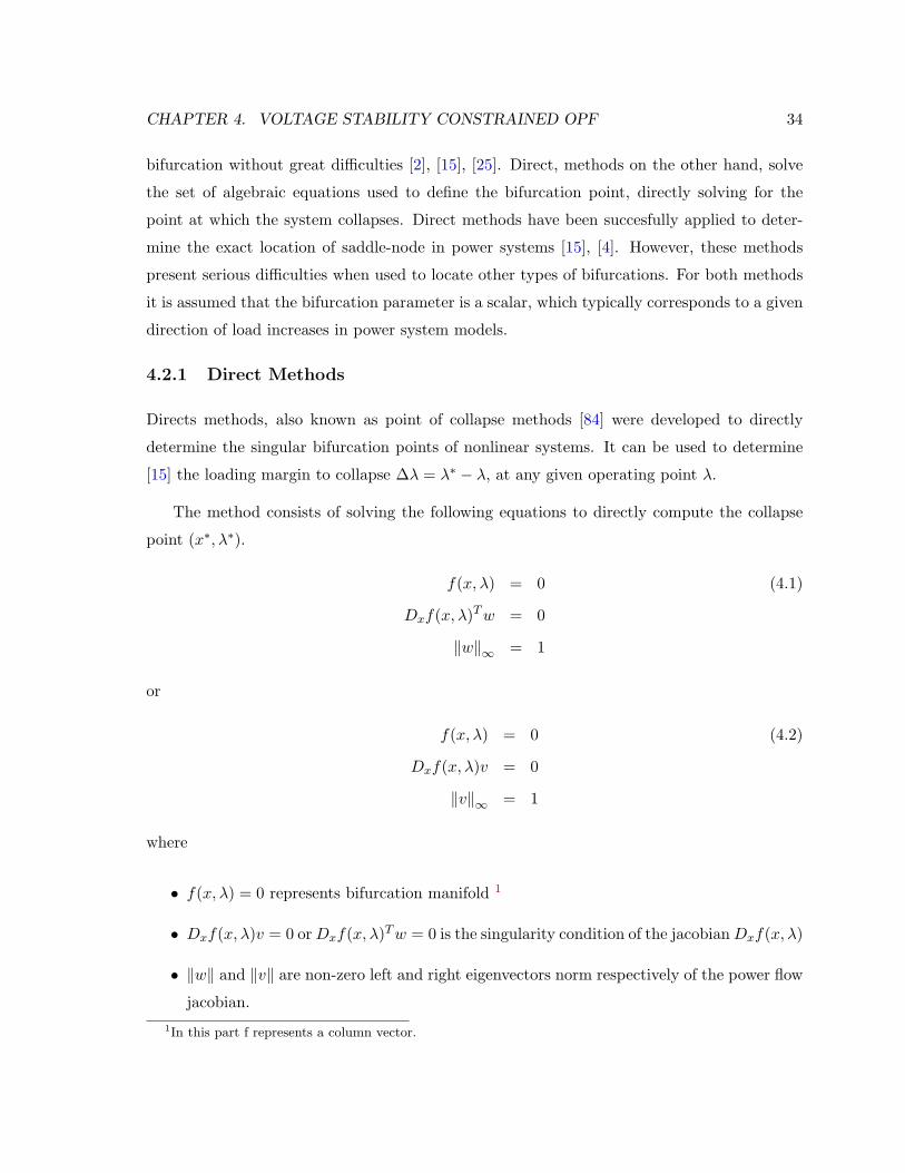
CHAPTER 4. VOLTAGE STABILITY CONSTRAINED OPF 34
bifurcation without great difficulties [2], [15], [25]. Direct, methods on the other hand, solve
the set of algebraic equations used to define the bifurcation point, directly solving for the
point at which the system collapses. Direct methods have been succesfully applied to deter-
mine the exact location of saddle-node in power systems [15], [4]. However, these methods
present serious difficulties when used to locate other types of bifurcations. For both methods
it is assumed that the bifurcation parameter is a scalar, which typically corresponds to a given
direction of load increases in power system models.
4.2.1 Direct Methods
Directs methods, also known as point of collapse methods [84] were developed to directly
determine the singular bifurcation points of nonlinear systems. It can be used to determine
[15] the loading margin to collapse ∆λ = λ∗ − λ, at any given operating point λ.
The method consists of solving the following equations to directly compute the collapse
point (x∗, λ∗).
f(x, λ) = 0 (4.1)
Dxf(x, λ)T w = 0
‖w‖∞ = 1
or
f(x, λ) = 0 (4.2)
Dxf(x, λ)v = 0
‖v‖∞ = 1
where
• f(x, λ) = 0 represents bifurcation manifold 1
• Dxf(x, λ)v = 0 or Dxf(x, λ)T w = 0 is the singularity condition of the jacobian Dxf(x, λ)
• ‖w‖ and ‖v‖ are non-zero left and right eigenvectors norm respectively of the power flow
jacobian.1In this part f represents a column vector.

CHAPTER 4. VOLTAGE STABILITY CONSTRAINED OPF 35
The nonsingular equations (4.1) and (4.2) correspond to the system’s steady state equa-
tions, the singularity condition at collapse point and nonzero eigenvector requirement for any
given system. Since J is singular at bifurcation point, a nonsingular eigenvector v or w must
be guaranteed. The loading margin has been observed to exhibit a linear and smooth behavior
[20].
The disadvantage of this approach is the high computational cost as the number of equa-
tions doubles with respect to the steady state equations. The other disadvantage of the direct
method as discussed in [15] and [68] is its inadequateness in predicting the collapse point when
limits such as generator reactive power limits may come into effect and henceforth. Also, the
requirement of good initial conditions for the eigenvectors, and the convergence problems as
the system approaches the collapse point due to significant change in eigenvalues and eigenvec-
tors. Another major disadvantage of direct method is its limitation of only detecting system
singularities (bifurcation). The continuation methods overcome these difficulties as explained
in the following section. Direct Methods which are implemented in PSAT allow to compute the
value of the loading parameter λ for at Saddle-Node Bifurcation points and at Limit-Induced
Bifurcation points. In PSAT, DMs can perform only “static” bifurcation analysis.
4.2.2 Continuation Methods
The Continuation method is used to find the bifurcations of the nonlinear equations similar to
the direct methods. The advantage of this method is its ability to not only find the bifurcation
point but also to trace the bifurcation manifold accurately. Consequently the voltage behavior
at all the system buses can be determined. Since, voltage profiles or PV nose curves are used
in some utilities to determine the proximity to voltage collapse, tracing their behavior over
different loading levels is an important observation.
The basic idea behind the continuation power flow technique is to use successive power
flow solutions to compute the voltage profile up to and beyond the collapse point. But,
continuation methods overcome the difficulties of successive power flow solution methods as
they are based on an augmented system model through parameterization. This allows to
trace complete voltage profile or bifurcation manifold without any problem, as parameter λ is
varied.
The technique implemented in the continuation is illustrated in Fig. 4.1, where a given

CHAPTER 4. VOLTAGE STABILITY CONSTRAINED OPF 36
x1
x2
∆x1
(x1,λ1)
(x2,λ2)(x0,λ0)
Figure 4.1: One Step of the Continuation method
equilibrium point (x1, λ1) is used to compute the direction vector ∆x1 and the change in
parameter ∆λ of the system. There are two steps involved in the process
1. Predictor and Parameterization : This step is known as the predictor, since it
generates an initial guess (x1 + ∆x1, λ1 + ∆λ1), which is then used to compute the new
equilibrium point (x2, λ2) in the corrector step.
Assuming the initial operating point (x1, λ1) is known and holds, taking partial
f(x1, λ1) = 0 (4.3)
derivatives yields,
df
dλ
∣∣∣∣(x1,λ1)
= Dxf(x1, λ1)dx
dλ
∣∣∣∣x=x1
+∂f(x, λ)
∂λ
∣∣∣∣x=x1
= 0. (4.4)
The tangent vector at that point is given by
τ =dx
dλ
∣∣∣∣x=x1
= −D−1x f(x1, λ1)
∂f(x, λ)∂λ
∣∣∣∣x=x1
(4.5)

CHAPTER 4. VOLTAGE STABILITY CONSTRAINED OPF 37
where Dxf(x1, λ1) represents power flow Jacobian. As the system approaches the bi-
furcation or collapse point, the system Jacobian becomes ill-conditioned and at the
bifurcation the Jacobian is singular, and hence in order to ensure that the tangent vec-
tor τ and numerical solution of the equations is well defined we need parameterization
of the predictor and corrector steps.
A. Step Length Control
The parameter step and the direction vector are found from the normalization of the
tangent vector found in the equation (4.5). The step generated by the predictor is given
by
∆x1
∆λ1= t1 (4.6)
Hence, one can choose
∆λ1 =k
‖t1‖(4.7)
∆x1 = kt
‖t1‖(4.8)
where k is a scalar positive constant that controls the size of the predictor step. This
normalization results in the reduction of the step size as the system approaches the
bifurcation point since the magnitude of tangent vector increases as the system gets
closer to this point. Therefore, steeper the curve, smaller is the step length. The
optimal values of step size k have been investigated by using the tangent vectors [30].
B. Parameterization
One of the simple technique used in [2], [15] is local parameterization, which consists
of interchanging the parameter λ with the system variable xi ∈ x that has the largest
normalized entry in the tangent vector, so that λ becomes part of the equations, whereas
xi becomes the new parameter p, i.e.,
p = maxi
∣∣∣∣∆xi
xi
∣∣∣∣ ,
∣∣∣∣∆λ
λ
∣∣∣∣ (4.9)
Detailed information regarding the predictors and parameterization techniques is given
in [20].
2. Corrector Step : The corrector step finds the actual point of solution (x2, λ2), gener-
ated from the predictor step point (x1+∆x1, λ1+∆λ1) with or without parameterization.

CHAPTER 4. VOLTAGE STABILITY CONSTRAINED OPF 38
Figure 4.2: Predictor and Corrector Steps in Continuation power flow
This solution can be obtained by solving the following set of equations for x and λ
f(x, λ) = 0 (4.10)
ρ(x, λ) = 0
From the Fig. 4.2, using a vector perpendicular to the tangent vector, we have
ρ(x, λ) =
∆x1
∆λ1
T x2 − x1 −∆x1
λ2 − λ1 −∆λ1
= 0 (4.11)
which can be written as,
ρ(x, λ) = ∆xT1 (x2 − x1 −∆x1) + ∆λ1(λ2 − λ2 −∆λ1) = 0 (4.12)
As shown in the Fig.(4.2), starting from point (x1, λ1) the above equations converge to
solution (x2, λ2)

CHAPTER 4. VOLTAGE STABILITY CONSTRAINED OPF 39
4.3 Multi Objective VSC-OPF Market model
The following optimization problem has been used in this work to represent an OPF based
market model with the inclusion of reactive power costs that helps investors and customers
in the establishment of reactive power market. The market model is designed in such a way
that system security is modeled through the use of voltage stability conditions.
Min. F = −p1
∑j∈J
BPj (PDj ) + BQj (PDj tan(φDj )) −∑i∈I
CPi(PSi)− CQi(QGi)
− p2λc
(4.13)
s.t. f(V, θ,QG, QD, PS , PD) = 0 → PF equations
fc(Vc, θc, QGc , λc, QD, PS , PD) = 0 → Max load PF equations
λcmin ≤ λc ≤ λcmax → Loading margin
PSmin ≤ PS ≤ PSmax → Supply bid blocks
PDmin ≤ PD ≤ PDmax → Demand bid blocks
Ihk(θ, V ) ≤ Ihkmax → Thermal limits
Ikh(θ, V ) ≤ Ikhmax
Ihk(θc, Vc) ≤ Ihkmax
Ikh(θc, Vc) ≤ Ikhmax
QGmin ≤ QG ≤ QGmax → Generator Q limits
QGmin ≤ QGc ≤ QGmax
Vmin ≤ V ≤ Vmax → Voltage “security” limits
Vmin ≤ Vc ≤ Vmax
A second set of power flow equations and constraints with a subscript c is introduced to
represent the system at the limit or “critical” conditions associated with the loading margin
λc in p.u., where λ is the parameter that drives the system to its maximum loading condition.
The maximum or critical loading point could be either associated with a thermal or bus voltage
limit or a voltage stability limit (collapse point) corresponding to a system singularity (saddle-
node bifurcation) or system controller limits like generator reactive power limits (limit-induced
bifurcation).
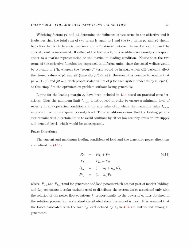
CHAPTER 4. VOLTAGE STABILITY CONSTRAINED OPF 40
Weighting factors p1 and p2 determine the influence of two terms in the objective and it
is obvious that the total sum of two terms is equal to 1 and the two terms p1 and p2 should
be > 0 so that both the social welfare and the “distance” between the market solution and the
critical point is maximized. If either of the terms is 0, this wouldnot necessarily correspond
either to a market representation or the maximum loading condition. Notice that the two
terms of the objective function are expressed in different units, since the social welfare would
be typically in $/h, whereas the “security” term would be in p.u., which will basically affect
the chosen values of p1 and p2 (typically p1>> p2 ). However, it is possible to assume that
p1 = (1 - p) and p2 = p, with proper scaled values of p for each system under study (0<p<1),
as this simplifies the optimization problem without losing generality.
Limits for the loading margin λc have been included in 4.14 based on practical consider-
ations. Thus the minimum limit λcmin is introduced in order to ensure a minimum level of
security in any operating condition and for any value of p, where the maximum value λcmax
imposes a maximum required security level. These conditions ensure that the loading param-
eter remains within certain limits to avoid soultions by either low security levels or low supply
and demand levels which would be unacceptable.
Power Directions:
The current and maximum loading conditions of load and the generator power directions
are defined by (4.14):
PG = PG0 + PS (4.14)
PL = PL0 + PD
PGc = (1 + λc + kGc)PG
PLc = (1 + λc)PL
where, PG0 and PL0 stand for generator and load powers which are not part of market bidding,
and kGc represents a scalar variable used to distribute the system losses associated only with
the solution of the power flow equations fc proportionally to the power injections obtained in
the solution process, i.e. a standard distributed slack bus model is used. It is assumed that
the losses associated with the loading level defined by λc in 4.14 are distributed among all
generators.

CHAPTER 4. VOLTAGE STABILITY CONSTRAINED OPF 41
4.3.1 Spot Pricing and Nodal Congestion Pricing
Spot Pricing
The Lagrangian multipliers associated with 4.14 correspond to the standard definition of LMPs
only when p = 0, i.e., for a pure market model. Lagrangian multipliers for p > 0 would lead
to unrealistic results, since they decrease almost linearly with respect to increases in p.
Consider the following vector objective function:
F =
−(BTP PD + BT
QPDtan(φD)− CTP PS − CT
QQG)
−λc
(4.15)
From a fundamental theorem of multi-objective optimization an optimal solution of 4.14 is also
a Pareto optimal point for the minimization problem constituted by the objective function
4.15 plus the constraints defined in 4.14 Thus, an optimal solution point of 4.14 has the
property of independently minimizing both terms of the objective function 4.15. Based on
this premise, for a given value of the weighting factor, say p∗, an optimization method is first
used to minimize the following Lagrangian function of 4.14

CHAPTER 4. VOLTAGE STABILITY CONSTRAINED OPF 42
Min. L = F − ρT f(θ, V,QG, QD, PS , PD) (4.16)
− ρT fc(θc, Vc, QGc , λc, QD, PS , PD)
− µλcmax(λcmax − λc)
− µλcmin(λc − λcmin)
− µTPSmax
(PSmax − PS)
− µTPSmin
(PS − PSmin)
− µTPDmax
(PDmax − PD)
− µTPDmin
(PD − PDmin)
− µTIhkmax
(Imax − Ihk)
− µTIkhmax
(Imax − Ikh)
− µTIhkcmax
(Imax − Ihkc)
− µTIkhcmax
(Imax − Ikhc)
− µTQGmax
(QGmax −QG)
− µTQGmin
(QG −QGmin)
− µTQGc max
(QGmax −QGc)
− µTQGc min
(QGc −QGmin)
− µTVmax
(Vmax − V )
− µTVmin
(V − Vmin)
− µTVc max
(Vmax − Vc)
− µTVc min
(Vc − Vmin)
Observe that the value of λc cannot be obtained by the mere solution of Sw, as its value
is basically defined by the value of p in the multi-objective problem 4.14. As a result, the
weighting factor p, although it affects the solution and the dual variables of it does not
explicitly appear in the equations. The solution provides the value of λ∗c associated with p∗
along with all other system variables and market bids.
Nodal Congestion Prices
Using the decomposition formula given in 3.2.2, the real power congestion price at each bus

CHAPTER 4. VOLTAGE STABILITY CONSTRAINED OPF 43
can be rewritten as follows:
NCP = [Dxf ]−1
∂Ihk
∂x(µIhkmax
− µIhkmin) +
0
µVmax − µVmin
(4.17)
Observe that NCPs in 4.17 depends only on shadow prices of dual variables µIhkmaxand µIhkmin
associated with current thermal limits, since the VSC-OPF model 4.14 does not include real
power flow limits as in 3.13. However, dependence on voltage security constraints given by
the inclusion of the “critical” system fc and on the loading parameter λc are implicit in 4.17.
4.3.2 Maximum Transfer Capability and Available Transfer Capability
The Available Transfer Capability (ATC) as defined by NERC, is a “measure of the transfer
capability remaining in the physical transmission network for further commercial activity over
and above already committed uses”[8]. This basic concept is typically associated with area
interchange limits used, for example, in markets for transmission rights.
In the multi-objective OPF approach λc represents the maximum loadability of the network
and, hence, this value can be viewed as a measure of the congestion of the network. Observe
that the maximum loading condition (MLC) or maximum transfer capability (MTC) and the
available loading capability (ALC) or available transfer capability (ATC) can be obtained as
a byproduct of the solution of 4.14:
MLC/MTC = (1 + λc)∑j∈J
PLj (4.18)
ALC/ATC = λc
∑j∈J
PLj = λcTTL
Contingencies are considered when computing λc, MLC and ATC based on real power flow
sensitivity analysis which is explained in next section.
4.4 N-1 Contingency Criterion
This section describes a technique for including in the Voltage Stability Constrained OPF
presented in 4.3 a N-1 contingency criterion. It is based on a sensitivity analysis of power flows
in transmission lines. The available transfer capability, locational marginal prices, reactive
power marginal prices and nodal congestion prices resulting from the solutions are compared
with results obtained by means of a standard OPF technique.

CHAPTER 4. VOLTAGE STABILITY CONSTRAINED OPF 44
4.4.1 VSC-OPF with Critical Line Contingency
Contingencies are included in 4.14 by taking out the selected lines when formulating the
“critical” power flow equations fc, thus ensuring that the current solution of the VSC-OPF
problem is feasible also for the given contingency. Thus, the VSC-OPF problem with N-1
contingency criterion is based on what has been proposed in [19], [61] and formulated as
follows:
Min. L = F − ρT f(θ, V,QG, QD, PS , PD) (4.19)
− ρT fN−1c (θc, Vc, QGc , λc, QD, PS , PD)
− µλcmax(λcmax − λc)
− µλcmin(λc − λcmin)
− µTPSmax
(PSmax − PS)
− µTPSmin
(PS − PSmin)
− µTPDmax
(PDmax − PD)
− µTPDmin
(PD − PDmin)
− µTIhkmax
(Imax − Ihk)
− µTIkhmax
(Imax − Ikh)
− µTIhkcmax
(Imax − Ihkc)
− µTIkhcmax
(Imax − Ikhc)
− µTQGmax
(QGmax −QG)
− µTQGmin
(QG −QGmin)
− µTQGc max
(QGmax −QGc)
− µTQGc min
(QGc −QGmin)
− µTVmax
(Vmax − V )
− µTVmin
(V − Vmin)
− µTVc max
(Vmax − Vc)
− µTVc min
(Vc − Vmin)
where fN−1c represent power flow equations for the system with under study with one line
outage. The techniques used in this thesis address the problem of determining efficiently the

CHAPTER 4. VOLTAGE STABILITY CONSTRAINED OPF 45
contingencies which cause the worst effects on the system, i.e. the lowest loading margin λc
and ATCN−1 (equation 4.20).
ATCN−1 = minh(λch− 1)TTLh (4.20)
where h indicates line outage.
4.4.2 Contingency Ranking with VSC-OPF
First, a basic VSC-OPF solution that does not consider contingencies is used for determining
the sensitivity of power flows with respect to the loading parameter λc. Then, based on this
solution and assuming a small variation ∈ of the loading parameter and recomputing the
power flows by solving fc, normalized sensitivity factors can be approximately computed as
follows:
phk = Phk∂Phk
∂λc≈ Phk(λc)
Phk(λc)− Phk(λc− ∈)∈
(4.21)
where phk and Phk are the sensitivity factor and the power flows of line h-k respectively. The
scaling is introduced for properly evaluating the “weight” of each line in the system, and thus
for considering only those lines characterized by both “significant” power transfers and the
high sensitivities [17].
The first lines with the biggest sensitivity factors phk are selected (from multiple tests, 5
lines appear to be a sufficient number), and a VSC-OPF for each one of these contingencies is
solved (may be done in parallel). The VSC-OPF solution that presents the lowest ATCN−1
is chosen as the final solution. Observe that not necessarily the outage of the line with the
highest sensitivity factor will always produce the lowest ATCN−1, because of the non-linear
nature of the voltage stability constraints. Hence the need of solving more than one VSC-
OPF problem. However, ranking the sensitivity factors leads generally to determine a reduced
number of critical areas; ATCN−1s associated with outages of high sensitivity lines within a
certain area generally show only small differences. Thus, in practice, one needs to evaluate
only one contingency constrained VSC-OPF for each critical area that was determined by the
sensitivity analysis.
Observe that line outages that cause a separation in islands of the original grid have to be
treated in a special way, since the VSC-OPF (4.3) may not converge. In order to solve this

CHAPTER 4. VOLTAGE STABILITY CONSTRAINED OPF 46
problem, the islanded market participants are not committed and the fixed power productions
and/or absorptions eliminated. This solution appears to be reasonable especially for realistic
transmission grids, which are typically well interconnected, as generally only very few buses
result islanded as the consequence of a line outage.
4.5 Summary
In this chapter, a multi-objective optimization for managing and pricing voltage stability
is explained. The multi-objective approach proposed by Milano [62] has been extended to
include the cost of reactive power in the social benefit so that more accurate signals for
ractive power pricing are obtained. The multi-objective OPF method allows market operators
and participants to directly control the desired level of system security by controlling the
weighting factors of the social welfare and loading margin, which is not possible in typical
security constrained OPF-based market implementations. A method based on power flow
sensitivities in the transmission lines to include N-1 contingency criterion is explained. The
VSC-OPF with N-1 contingency is considered as the base case to compare the results with
VAR support.

Chapter
5
VAR Support and Pricing
5.1 Introduction
The transfer of real power can not be realized without reactive power/voltage support. Reac-
tive power plays an important role in supporting the real power transfer. This support becomes
especially important when an increasing number of transactions are utilizing the transmission
system and voltages become a bottleneck in preventing additional power transfer. Establish-
ing a price structure for reactive power and its support is important both operationally and
financially. Considering the high costs of VAR support, it is important to find the optimal
size and location of VAR support.
5.2 SVC Investment Costs
The following total investment cost analysis for static var compensator is based on information
from Siemens AG database [39]. According to the data given, costs can be approximated by
CSV C = 0.0003 s2 − 0.3051 s + 127.38 (US $/KVAr) (5.1)
where Csvc is in (US $/KVAr) and s is the operating range of the SVC in MVAR. The plot
of the cost function against operating range upto 400 MVAR is shown in Fig. 5.1.
47

CHAPTER 5. VAR SUPPORT AND PRICING 48
Figure 5.1: SVC Investment costs
5.2.1 Equipment Costs and Infrastructure Costs
As described in [39] the investment costs of FACTS devices can be split into two categories
1. Device equipment costs
2. Necessary Infrastructure costs
Equipment costs depend not only upon the installation rating but also upon special re-
quirements such as:
• Redundancy of the control and protection systems
• Seismic conditions
• Ambient conditions (e.g. temperature, pollution level), and
• Communication requirements with the substation control system or the regional or na-
tional control center.
Infrastructure costs depend on the device’s and costs include
• Land acquisition, if there is insufficient space in the existing substation,

CHAPTER 5. VAR SUPPORT AND PRICING 49
• Modifications to the existing substation,
• Construction of a building for indoor equipment,
• Yard civil works, and
• Communication infrastructure.
The typical range of investment costs is shown in Fig. 5.2, [39] with both the lower and
upper limits of the cost areas. The lower limit of the cost area indicates the equipment costs
and the upper limit indicates the total investment costs including the infrastructure costs. In
this study, the total investment costs, corresponding to the upper limit of the Fig. 5.2 are used.
The operating costs of SVC are generally negligible when compared to the total investment
costs and can be safely ignored.
Figure 5.2: Typical Investemnt Costs for SVC / STATCOM [39]
Most of the FACTS devices are in service for many years [39] and only a part of their life
time is employed in regulation of power flow [13]. Since SVC procurement requires a lot of
capital cost, decision on investment needs to be based on the returns the device will allow. In
this study, the annual cost of the device is calculated by assuming a uniform interest rate of
6% and 15 years of life expectancy. Hence, the annualized cost of the SVC as calculated from

CHAPTER 5. VAR SUPPORT AND PRICING 50
the model shown in Fig. 5.1 and from equation (5.1) is
Annual Csvc =P · r · (1 + r)n
(1 + r)n − 1(5.2)
Costsvc =Annual Csvc
8760(US $/hr) (5.3)
where P, r, and n denote principal value, interest rate per payment, and number of payments
respectively. Csvc is the total investment costs of the SVC given from equation (5.1).
5.3 Optimal Placement of VAR Support Devices
According to engineering economics, whenever there are different investment schemes, techni-
cal and economic quantitative analysis should be performed and economic assessment should
be provided in order to select the optimal scheme. The OPF solution will give the amount of
reactive power support needed at each load bus. It is necessary to use cost-benefit analysis
(CBA) to analyze whether the new VAR source would be cost-effective when it is actually
installed.
5.3.1 Cost Benefit Analysis
For VAR planning purposes, costs and sites of reactive power sources must be determined.
This thesis also presents a new method to select the reactive power source sites by the ana-
lytic hierarchy process (AHP). The proposed approach comprehensively considers the network
topology, operation states and reactive power support service cost of each candidate VAR
source site. Specifically it considers the social welfare benefit-to-cost ratio (SBCR), maxi-
mum loading condition benefit-to-cost ratio (MBCR) and congestion cost benefit-to-cost ratio
(CBCR) based on a cost - benefit analysis. Due to their independent nature, results from
these three BCRs are not necessarily the same. Of course, all BCRs reflect the improvement
of the systems operation state after the VAR support service is provided.
Unfortunately, it is difficult to find a unified process for ranking these results. Moreover, all
BCRs have not included other qualitative relationships for considering relative importance of
different VAR source sites. AHP is a simple and convenient method to analyze a complicated
problem (or a complex system). It is especially suitable for problems which are very difficult
to be analyzed whole quantitatively, and is now widely used in various areas [83] including

CHAPTER 5. VAR SUPPORT AND PRICING 51
power systems. AHP can help to quantify the decision-makers thinking. Thus, it provides
a useful means for considering myriad factors in the ranking and selection of VAR source
locations. The method is explained in detail in the next section.
The aim of reactive power planning is to obtain optimal VAR placement scheme (location
and sizing of SVC on the load buses) under the some load level and constraints. In this work,
multi-objective OPF formulation is used along with the investment costs of SVC for this
purpose. Considering the ‘social welfare’ objective function, somewhat higher losses would be
incurred since cheaper generating sources, generally located away from load center, would be
predominantly used to meet the demands. However, it might be worthwhile for the utility to
bear this additional loss rather than switch generation to relatively expensive units located
nearer to load center [24]. The OPF formulation as explained in the previous chapter is
extended to include cost of VAR support/SVC is given in equation 5.4.
Min. F = −p1 ∗ social welfare− p2 ∗ λc + CsvcQsvc (5.4)
where F is the sum of social welfare ($/h), loading margin (p.u) and total investement cost
of SVC ($/h).
In order to reflect the overall benefits after SVC is installed, three kinds of BCR were
considered for the selection of optimal location.
(1) Social welfare benefit-to-cost ratio (SBCR) ($/h)
SBCR =max(0,
24∑t=1
(Sw(Qsvci)− Sw(0)))
C(Qsvci)(5.5)
or
SBCRt =max[0, (St
w(Qsvci)− Stw(0))]
C(Qsvci)/24(5.6)
where: Stw(0), the social welfare at time t before SVC at bus i is installed; St
w(Qsvci), the social
welfare at time t after SVC at bus i is installed; C(Qsvci), the equivalent daily investment
cost of SVC at load node i ($/day). Because of the chosen objective at some load buses the
social welfare may decrease after the SVC is installed though the loading margin of the system
increase. Since the social welfare being the main objective of the market opearator placement
of SVC at such load buses is not desired. This means, Stw(0) may be larger than St
w(Qsvci),

CHAPTER 5. VAR SUPPORT AND PRICING 52
i.e. (Stw(Qsvci) − St
w(0)) is negative. In other words no social welfare benefit is obtained in
this case. Therefore, it is defined as SBCRt = 0 to reflect this case, i.e.
max[0, (Stw(Qsvci)− St
w(0))] = 0 (5.7)
(2) Maximum loadability benefit-to-cost ratio (MBCR) (MW/h)
MBCR =(
24∑t=1
(ML(Qsvci)−ML(0)))
C(Qsvci)(5.8)
or
MBCRt =(MLt(Qsvci)−MLt(0))
C(Qsvci)/24(5.9)
where: ML(0) is the loading margin or maximum loadability of the system at time t before
SVC at bus i is installed and ML(Qsvci) is the loading margin at time t after SVC at bus i
is installed. MBCR provides the increase in maximum loading condition with the installation
of SVC
(3) Congestion cost benefit-to-cost ratio (CBCR) ($/h)
CBCR =max(0,
24∑t=1
(CC(0)− CC(Qsvci)))
C(Qsvci)(5.10)
or
CBCRt =max[0, (CCt(0)− CCt(Qsvci))]
C(Qsvci)/24(5.11)
where: CCt(0) is the congestion cost at time t before SVC at bus i is installed and CCt(Qsvci)
is the congestion cost at time t after SVC at bus i is installed; C(Qsvci), the equivalent daily
investment cost of SVC at load node i ($/day).
Obviously, all BCRs reflect the improvement of the system operation state after the VAR
support service is provided. However, the ranking results from these three BCRs might not
be same due to their independent nature. The relative importance of each factor over other
is represented as weighting factor which is found through analytic hierarchy process.
The index for optimal placement of VAR support is formulated as:
J = maxi∈NL
J i = w1 J i1 + w2 J i
2 + w3 J i3 (5.12)

CHAPTER 5. VAR SUPPORT AND PRICING 53
where all the factors are evaluated at each optimal location i for a selected critical line con-
tingency found through sensitivity analysis.
J = Index to be maximized
J1 = Normalized value of SBCRs
J2 = Normalized value of MBCRs
J3 = Normalized value of CBCRs
NL = Total number of load buses
w1 + w2 + w3 = 1
The bus corresponding to the maximum value of index J is the optimal site for installing
SVC. First compute the VSC-OPF solution by reading the network topology and market data
. Identify the critical line such that the system’s overall available transfer capability (ATC)
reaches minimum with the line outage. This index is suitable for the systems which are
capable of maintaining minimum level of security after critical line outage. The new benefits
with SVC are obtained at each load bus over a period of 24 hours and all the three BCRs
can be calculated from equations 5.6, 5.9, and 5.11. The importance of each factor over other
factor is calculated by setting up an AHP model for source selection.
If the system cannot be loaded to the minimum desired security level i.e. 110% of system
base load, it is considered as the market solution is not feasible i.e base case solution is not
existing and it is a necessity for the system to install additional VAR support to make system
realiable, secure and stable. For such systems the index for optimal VAR source site is given in
5.13. Considering the three factors social welfare, maximum loading condition and congestion
cost for all the load buses. The index is given below,
J = maxi∈NL
J i = w1 J i1 + w2 J i
2 − w3 J i3 (5.13)
where, the Social welfare is obtained from:
J1 =
24∑t=1
Sw(Qsvci)
C(Qsvci)(5.14)
or
J1t =
Stw(Qsvci)
C(Qsvci)/24(5.15)

CHAPTER 5. VAR SUPPORT AND PRICING 54
Maximum loading condition or system loadability:
J2 =
24∑t=1
ML(Qsvci)
C(Qsvci)(5.16)
or
J2t =
MLt(Qsvci)C(Qsvci)/24
(5.17)
Congestion cost:
J3 =
24∑t=1
CC(Qsvci)
C(Qsvci)(5.18)
or
J3t =
CCt(Qsvci)C(Qsvci)/24
(5.19)
Setting up an AHP model and ranking the source sites can be performed similar to previous
case. The maximum social welfare, MLC & CC with SVC at load buses can be obtained from
equations 5.15, 5.17 and 5.19 respectively. The bus corresponding to the maximum value of
J is chosen as the optimal location.
In the equations 5.15, 5.17and CC 5.19, the final values are then obtained through nor-
malization by dividing all the values with the maximum.
J = Index to be maximized
J1 = Normalized value of J1
J2 = Normalized value of J2
J3 = Normalized value of J3
NL = Total number of load buses
w1 + w2 + w3 = 1
The sum of total weights is equal to 1, so the resultant weights have values ranging from 0 to
1.
5.3.2 Analytic Hierarchy Process
The principle of the analytic hierarchy process is that first a structural model of the analytic
hierarchy is established through analysis of the complex system, then the complex problem

CHAPTER 5. VAR SUPPORT AND PRICING 55
is transformed into the problem of rank calculation within the hierarchy structure. In the
ranking computation, the ranking in each hierarchy can also be converted into the judgment
and comparison of a series of pairs of factors. This implies that a judgment matrix is needed
to reflect these judgments and comparisons. The judgment matrix can be formed according
to the quantified judgment of pairs of factors using some ratio scale method. Consequently,
the value of the weighting coefficients of all factors can be obtained through calculating the
maximal eigenvalue and the corresponding eigenvector of the judgment matrix. Obviously, the
purpose of ranking the elements of the eigenvector corresponding to the maximal eigenvalue
is simply to obtain the weight of each factor among the different kinds of factors.
The steps of the AHP algorithm may be written as follows:
1. Set up a hierarchy model.
2. Form a judgment matrix.
The value of elements in the judgment matrix reflects the users knowledge about the
relative importance between every pair of factors.
3. Calculate the maximal eigenvalue and the corresponding eigenvector of the judgment
matrix.
4. Perform hierarchy ranking and consistency checking of results.
We can perform the hierarchy ranking according to the value of elements in the eigenvector,
which represents the relative importance of the corresponding factor. The consistency index
(CI) of a hierarchy ranking is defined as
CI =(λmax − n)
(n− 1)(5.20)
where λmax is the maximal eigenvalue of the judgment matrix and n is the dimension of the
judgment matrix.
The stochastic consistency ratio is defined as
CR =CI
RI(5.21)
where RI is a set of given average stochastic consistency indices.

CHAPTER 5. VAR SUPPORT AND PRICING 56
n = 1 n = 2 n = 3 n = 4 n = 5 n = 6 n = 7 n = 8 n = 9
0.00 0.00 0.58 0.90 1.12 1.24 1.32 1.41 1.45
Table 5.1: Set of average stochastic consistency indices RI
Figure 5.3: Hierarchy model for optimal placement of SVC
For any judgment matrix of dimension 1 to 9, the average stochastic consistency indices
RI, given in Table 5.1, can be obtained according to statistical calculations. A satisfactory
hierarchy ranking has been obtained when the stochastic consistency ratio CR < 0.1.
Hierarchy model of VAR placement
The hierarchy model for the VAR placement is simple. It consists of only a two-level hierarchy
as shown in Fig. 5.3. In this way, the calculation of the weighting coefficients in the objective
for VAR location is changed into ranking calculation in the hierarchy model. Thus, it is
necessary to form a judgement matrix A for ranking computation. According to the principle
of AHP mentioned above, the judgement matrix is formed as below 5.22.
A =
W1/W1 W1/W2 W1/W3
W2/W1 W2/W2 W2/W3
W3/W1 W3/W2 W3/W3
(5.22)
where Wi is the weighting coefficient of the ith subobjective in the hierarchy model. Of course
Wi, which is just what we need, is unknown.
Wi/Wj can be obtained according to the experiences of electrical engineers using some
ratio scale methods. The weights usually consist of numbers on a scale of ‘1-9’, as illustrated
in Table [5.2]. For example, if J2 as compared to J1 is “clearly more important”, corresponding
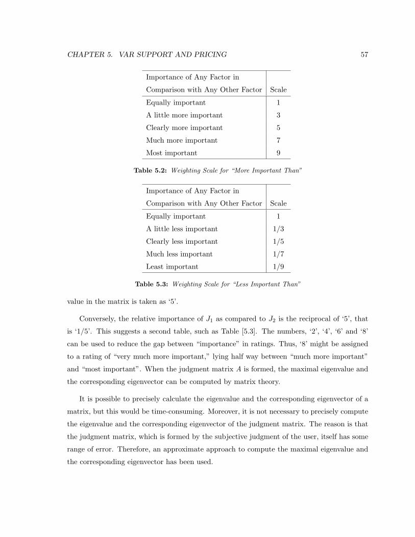
CHAPTER 5. VAR SUPPORT AND PRICING 57
Importance of Any Factor in
Comparison with Any Other Factor Scale
Equally important 1
A little more important 3
Clearly more important 5
Much more important 7
Most important 9
Table 5.2: Weighting Scale for “More Important Than”
Importance of Any Factor in
Comparison with Any Other Factor Scale
Equally important 1
A little less important 1/3
Clearly less important 1/5
Much less important 1/7
Least important 1/9
Table 5.3: Weighting Scale for “Less Important Than”
value in the matrix is taken as ‘5’.
Conversely, the relative importance of J1 as compared to J2 is the reciprocal of ‘5’, that
is ‘1/5’. This suggests a second table, such as Table [5.3]. The numbers, ‘2’, ‘4’, ‘6’ and ‘8’
can be used to reduce the gap between “importance” in ratings. Thus, ‘8’ might be assigned
to a rating of “very much more important,” lying half way between “much more important”
and “most important”. When the judgment matrix A is formed, the maximal eigenvalue and
the corresponding eigenvector can be computed by matrix theory.
It is possible to precisely calculate the eigenvalue and the corresponding eigenvector of a
matrix, but this would be time-consuming. Moreover, it is not necessary to precisely compute
the eigenvalue and the corresponding eigenvector of the judgment matrix. The reason is that
the judgment matrix, which is formed by the subjective judgment of the user, itself has some
range of error. Therefore, an approximate approach to compute the maximal eigenvalue and
the corresponding eigenvector has been used.

CHAPTER 5. VAR SUPPORT AND PRICING 58
Sum Method:
(i) Normalize every column in the judgement matrix:
X∗ij =
Xij∑k
Xkji, j, k = 1, 2, ..., n (5.23)
Now, the judgment matrix A is changed into a new matrix A∗, in which each column has been
normalised.
(ii) Add all the elements of each row in matrix A∗:
W ∗i =
∑j
Xij i, j, k = 1, 2, ..., n (5.24)
(iii) Normalize the vector W ∗, which equals [W ∗1 ,W ∗
2 , ...,W ∗n ]T
Wi =W ∗
i∑j
W ∗j
i, j, k = 1, 2, ..., n (5.25)
Hence, we obtain the eigenvector of the judgment matrix A:
W = [W1,W2, ...,Wn]T (5.26)
(iv) Calculate the maximal eigenvalue of the judgment matrix λmax:
λmax =∑
i
[(AW)i
nWi
]i = 1, 2, ..., n (5.27)
where (AW)i represents the ith element in vector AW.
5.3.3 Pricing VAR Support Services
FACTS devices are being used in many places to relieve congestion, to improve system load-
ability and there is a potential price reduction upon its usage. A pricing scheme for FACTS
devices which are used in congestion relief and increase in social welfare, so that new con-
struction can be efficiently simulated, is still missing. The effects of FACTS devices are not
constrained to the location where they are installed and are hard to measure by the power
flowing through them. Since the costs associated with FACTS controllers are high, pricing
methodologies for the services provided by these controllers should be developed.

CHAPTER 5. VAR SUPPORT AND PRICING 59
The pricing methods are based on a comparison of congestion costs and social welfare.
The congestion costs are defined as:
CC =∑
(LMPiPdi+ RMPiPdi
tan(φdi)) −
∑(LMPjPsj + RMPjQgj ) (5.28)
where CC is the congestion cost in $/h, LMP is the locational marginal price for demand
bus i or supply bus j in $/MWh, and Pdi& Psj are the demand and supply powers in MW.
Thus any reduction in CC due to the application of FACTS is considered to be a profit which
cannot exist without these devices. Consequently, the difference between the CC with and
without the FACTS devices is used to price the reactive services of the device.
FP = CC|wof − CC|wf (5.29)
where FP is FACTS pricing in $/h, and CC|wof and CC|wf are the congestion costs without
and with FACTS device in service respectively. The value of FP is not considerable if the
system is not heavily loaded.
The social welfare Sw can also be used as a tool for pricing the FACTS service. It is
defined as:
SP = SP |wf − SP |wof (5.30)
where SP is the social welfare price in $/h and SP |wof and SP |wf are the social welfare
without and with FACTS device in service respectively. Similar to FP, the value of SP is not
considerable if the system is not heavily loaded.
5.3.4 Analysis of Reactive Power Pricing
Developing an accurate and feasible method for reactive power pricing is important in the
electricity market, Such reactive power price cannot be obtained by conventional optimal power
flow models because the production cost of reactive power is ignored in these models. It is
realized that establishing an accurate pricing structure of reactive power can not only recover
the costs of reactive power providers, but also provide economic information for real-time
operations. In this thesis, a social welfare objective function with both supply and demand
reactive power costs are considered. Tests under different system operating conditions help to
observe how those conditions influence reactive power prices.

CHAPTER 5. VAR SUPPORT AND PRICING 60
Reactive power production cost can be represented as the opportunity cost of generator.
According to the loading capability diagram of a generator, reactive power output may re-
duce active power output capacity of generators which can at least serve as spinning reserve,
therefore causes implicit financial loss to generators. Actually, opportunity cost depends on
the real time balance between demand and supply in the market, so it is difficult to determine
the real value. The opportunity cost (5.31) in general is approximated as:
Cpgi(QGi) =[Cpgi(SGi,max) −
√Cpgi(SGi,max)2 −Q2
Gi
].k (5.31)
where SGi,max is the nominal apparent power of the generator at bus i ; QGi is the reactive
power output of the generator at bus i ; k is the profit rate of of active power generation,
usually between 5% and 10%.
Since, there is no similar model for the reactive power procurement cost on the demand
side and in addition to make the calculations simple, the cost to produce and consume reac-
tive power is taken as a percentage of its respective real power bid price without losing any
generality.
5.4 VSC-OPF with SVC and N-1 contingency criterion
The important objective of this thesis work is to study the effect of SVC on spot pricing in a
VSC-OPF based market model. The multi-objective includes maximization of social welfare,
maximum distance to collapse and the cost of SVC in $/h. While calculating the loading
margin the N-1 contingency criterion is considered.
Static VAR Compensator (SVC):
SVC is used for voltage control applications in transmission systems. The placement of
SVC has been considered at load bus only but not in the middle of the line, since the benefits
rendered by SVC in the network go in vain with the line outage. Reactive power output of
an SVC (QSV C) lies within limits set by available inductive and capacitive susceptances (Bind
and Bcap respectively) as follows:
Qind = BindV2ref (5.32)
Qcap = BcapV2ref (5.33)
Qmin ≤ QSV C ≤ Qmax (5.34)

CHAPTER 5. VAR SUPPORT AND PRICING 61
Where Vref is the reference voltage magnitude at SVC node. In the OPF formulation, steady
state model of SVC has been taken as a PV generator with P = 0 and supply reactive power
with the above set reactive power limits. The investment costs of SVC are given in section 5.2
5.5 Summary
An index to place the VAR support in the network considering both technical and economical
factors is proposed based on CBA. Various factors such as social welfare, maximum loading
condition and congestion cost are computed in a voltage-stability constrained OPF. AHP
method is used to find the quantitative relationship between the three BCRs taking into
account the complete network topology. A simple method to price VAR support to recover
the investment cost is proposed.

Chapter
6
System Studies and Discussion
6.1 Test Systems Description
This chapter describes two case studies, the first case maintains minimum level of security
after N-1 contingency and the second system fails to maintain minimum level of security.
1. Six-Bus Test System: Fig. 6.1 depicts the six-bus test system single-line diagram, which
is extracted from [85].
2. IEEE 14-Bus Test System: A single-line diagram of the IEEE 14-bus test system is
depicted in Fig. 6.10 which represents a portion of the American Electric Power System
(in the Midwestern US) obtained from [94]
In sections 6.2 and 6.3, the OPF problem for 3.13 and 4.3 are applied to the two test
systems and compared the effect of system security on power dispatch and electricity prices.
The power flow limits needed in 3.13 were obtained “offline” by means of a continuation
power flow technique [20]. For both test systems, bid load and generator powers were used as
the direction needed to obtain a maximum loading point and the associated power flows in
the lines, ignoring contingencies so that proper comparisons can be made. The limits of the
62

CHAPTER 6. SYSTEM STUDIES AND DISCUSSION 63
loading parameter were assumed to be λcmin = 0.1 and λcmax = 0.8 (i.e., for any value of p, it
is assumed that the system can be securely loaded to an MLC between 110% and 180% of the
total transaction level of the given solution). To allow for adequate comparisons, the actual
power flow limits used in 3.13 were reduced by 10% with respect to the values obtained from
the offline continuation power flow analysis to emulate the λc = 0.1 limit.
VSC-OPF is extended to include N-1 contingency criterion and the critical line is iden-
tified through power transfer sensitivity analysis. Optimal scheme for placing VAR support
explained in section 5.3 is implemented by performing AHP analysis to find the appropriate
weights for economical and technical terms. The results are then compared with Standard
OPF and VSC-OPF with N-1 contingency and no VAR support. Transmission prices before
and after the VAR support are compared for 6-bus test system as the system can be securely
loaded and stable after crtical line failure. The effect of weighting factor p on the total trans-
action level, congestion costs and the maximum loading margin λc for the system with SVC
is observed.
The IEEE 14-bus test system is not stable with critical line failure and therefore it needs
VAR support to avoid voltage collapse and increase loading margin in this particular case.
The index given in 5.13 is used for optimal placement of VAR support. The effect of SVC on
power dispatch and electricity prices are compared with standard OPF, the case without SVC
and without N-1 contingency criterion. The transmission prices are calculated using wheeling
charges method. Reactive power marginal prices are effected because of the inclusion of cost
for both suppliers and consumers. Though, there is some debate regarding the viability of
reactive power prices, any pricing scheme will likely to be based on spot pricing technique.
The impact of load power factor on reactive power marginal prices is analysed.
6.2 6-Bus Test System
The system represents three generation companies (GENCOs) and three energy supply compa-
nies (ESCOs) that provide supply and demand bids. The complete data set for this system is
provided in the Appendix A.1.2, so that the results discussed here may be readily reproduced.

CHAPTER 6. SYSTEM STUDIES AND DISCUSSION 64
Figure 6.1: 6-bus test system [85]

CHAPTER 6. SYSTEM STUDIES AND DISCUSSION 65
Pariticipant V LMP RMP NCP PBID P0 Pay
[p.u.] [$/MWh] [$/MVArh] [$/MWh] [MW] [MW] [$/h]
GENCO1 1.089 9.70 0.97 1.24 14.5 90 -811
GENCO2 1.091 8.42 0.88 0.00 0.0 140 -907
GENCO3 1.100 7.00 0.70 -1.03 20.5 60 -496
ESCO4 1.034 11.91 1.38 3.41 25.3 90 1184
ESCO5 1.037 10.45 1.15 1.09 2.3 100 870
ESCO6 1.055 9.57 0.81 1.79 6.4 90 746
Totals T = 243.98 MW Congestion Cost = 584.85 $/h
Losses = 6.23 MW
Table 6.1: Six-bus test system: OPF with offline power flow limits
6.2.1 Results and Discussion
The results for the standard OPF formulation (3.13) are reported in Table 6.1. The results
depict that the system is having low transaction level ‘T’ and heterogeneous LMPs, RMPs
and NCPs, indicating that the system constraints, and in particular active power flow limits,
negatively affect the market solution. Table 6.1 shows also the total losses and the payment
given to the Independent Market Operator (referred to as PayIMO) or Congestion Cost (CC),
which is computed as the difference between demand and supply payments.
Table 6.2 illustrates the initial solution of the VSC-OPF problem 4.3. The weighting factor
p in the objective function of VSC-OPF used for maximizing the loading parameter, was set
to p = 10−3 as this was determined to be a value that does not significantly affect the market
solution, since the distance to the maximum loading point is not being really “optimized,”
with mostly the social welfare being considered in the objective function. Observe that, as
expected, the absence of active power flow limits and contingencies makes possible a higher
total transaction level ‘T’ and more homogeneous LMPs, RMPs and lower NCPs. For both
solutions, generator voltages are almost at their maximum limits, as expected, since this
condition generally provides higher transactions levels.
The improved LMPs result also in a lower total price paid to the independent market
operator (PayIMO) (i.e., the network congestion prices are lower), even though the system
losses are higher which is expected, as ‘T’ is higher. This demonstrates that offline power flow

CHAPTER 6. SYSTEM STUDIES AND DISCUSSION 66
Pariticipant V LMP RMP NCP PBID P0 Pay
[p.u.] [$/MWh] [$/MVArh] [$/MWh] [MW] [MW] [$/h]
GENCO1 1.096 9.20 0.97 0.01 0.0 90 -650
GENCO2 1.100 9.08 0.88 0.00 37.5 140 -1324
GENCO3 1.100 9.15 0.70 0.01 30.0 60 -721
ESCO4 1.033 9.76 1.29 0.28 37.5 90 1106
ESCO5 1.033 9.76 1.21 0.31 15.0 100 951
ESCO6 1.054 9.48 0.99 0.19 12.2 90 806
Totals T = 274.72 MW Congestion Cost = 168.96 $/h
Losses = 7.93 MW Loading Margin = 0.73
MLC = 474.16 MW
Table 6.2: Six-bus test system: VSC-OPF w/o contingencies
Line # Line h− k Phk(λ) (p.u.) phk=Phk*dPhk/dλ (106) ATCN−1 (MW)
1 2-3 0.127 0.0025 184.71
2 3-6 0.932 0.1897 77.85
3 4-5 0.032 0.0008 184.38
4 3-5 0.530 0.0419 155.09
5 5-6 0.098 0.0009 179.25
6 2-4 1.324 0.2531 27.47
7 1-2 0.043 0.0117 191.71
8 1-4 0.655 0.1073 42.61
9 1-5 0.506 0.0318 174.17
10 2-6 0.599 0.1189 132.58
11 2-5 0.491 0.0581 151.02
Table 6.3: Six-bus test system: Sensitivity coefficients Phk and ATC (N-1)
limits are not adequate constraints for representing the actual system congestion and not a
very good reprentation of stability.
Table 6.3 shows the coefficients phk used for sensitivity analysis. As mentioned in section
4.4, the line which produces lowest ATCN−1 is chosen as the critical line. For the six-bus test
system failure of ‘line 6’ i.e. line connecting from bus 2 - bus 4 produces the lowest ATC.
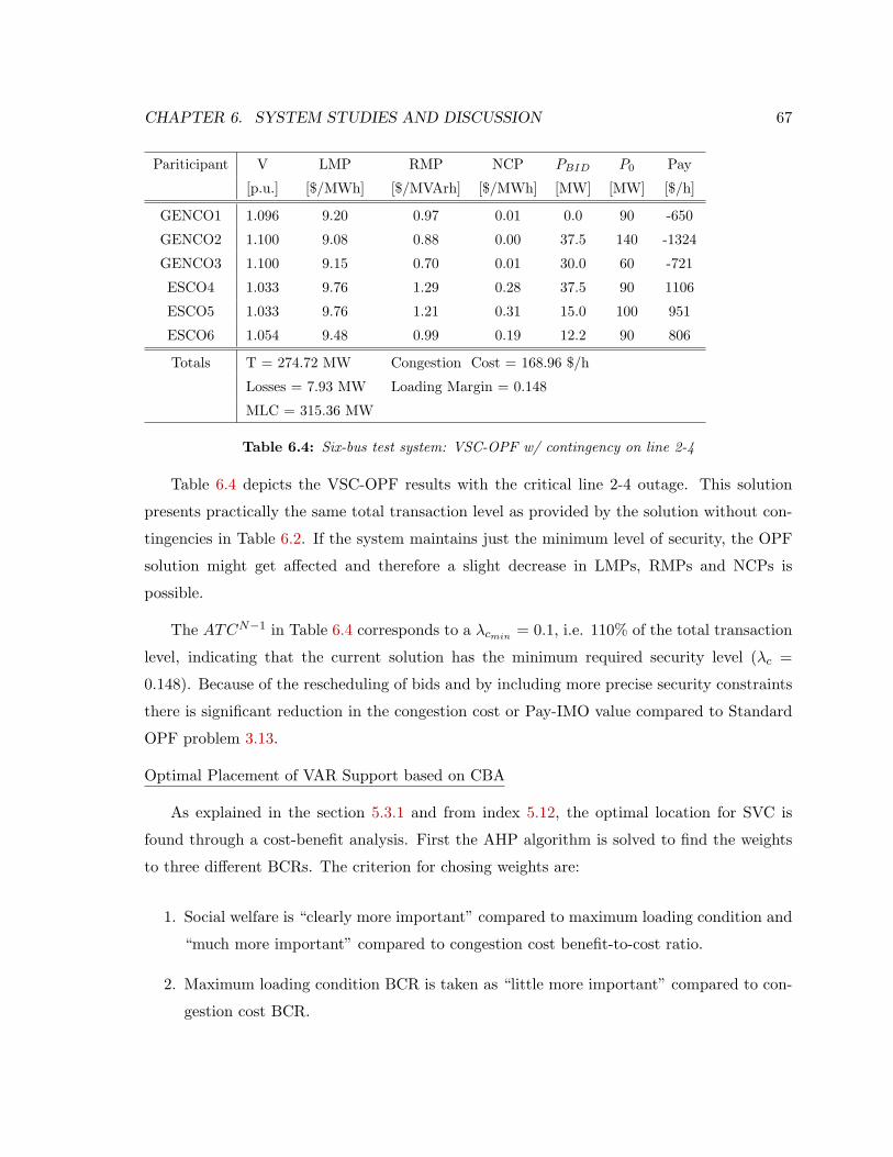
CHAPTER 6. SYSTEM STUDIES AND DISCUSSION 67
Pariticipant V LMP RMP NCP PBID P0 Pay
[p.u.] [$/MWh] [$/MVArh] [$/MWh] [MW] [MW] [$/h]
GENCO1 1.096 9.20 0.97 0.01 0.0 90 -650
GENCO2 1.100 9.08 0.88 0.00 37.5 140 -1324
GENCO3 1.100 9.15 0.70 0.01 30.0 60 -721
ESCO4 1.033 9.76 1.29 0.28 37.5 90 1106
ESCO5 1.033 9.76 1.21 0.31 15.0 100 951
ESCO6 1.054 9.48 0.99 0.19 12.2 90 806
Totals T = 274.72 MW Congestion Cost = 168.96 $/h
Losses = 7.93 MW Loading Margin = 0.148
MLC = 315.36 MW
Table 6.4: Six-bus test system: VSC-OPF w/ contingency on line 2-4
Table 6.4 depicts the VSC-OPF results with the critical line 2-4 outage. This solution
presents practically the same total transaction level as provided by the solution without con-
tingencies in Table 6.2. If the system maintains just the minimum level of security, the OPF
solution might get affected and therefore a slight decrease in LMPs, RMPs and NCPs is
possible.
The ATCN−1 in Table 6.4 corresponds to a λcmin = 0.1, i.e. 110% of the total transaction
level, indicating that the current solution has the minimum required security level (λc =
0.148). Because of the rescheduling of bids and by including more precise security constraints
there is significant reduction in the congestion cost or Pay-IMO value compared to Standard
OPF problem 3.13.
Optimal Placement of VAR Support based on CBA
As explained in the section 5.3.1 and from index 5.12, the optimal location for SVC is
found through a cost-benefit analysis. First the AHP algorithm is solved to find the weights
to three different BCRs. The criterion for chosing weights are:
1. Social welfare is “clearly more important” compared to maximum loading condition and
“much more important” compared to congestion cost benefit-to-cost ratio.
2. Maximum loading condition BCR is taken as “little more important” compared to con-
gestion cost BCR.
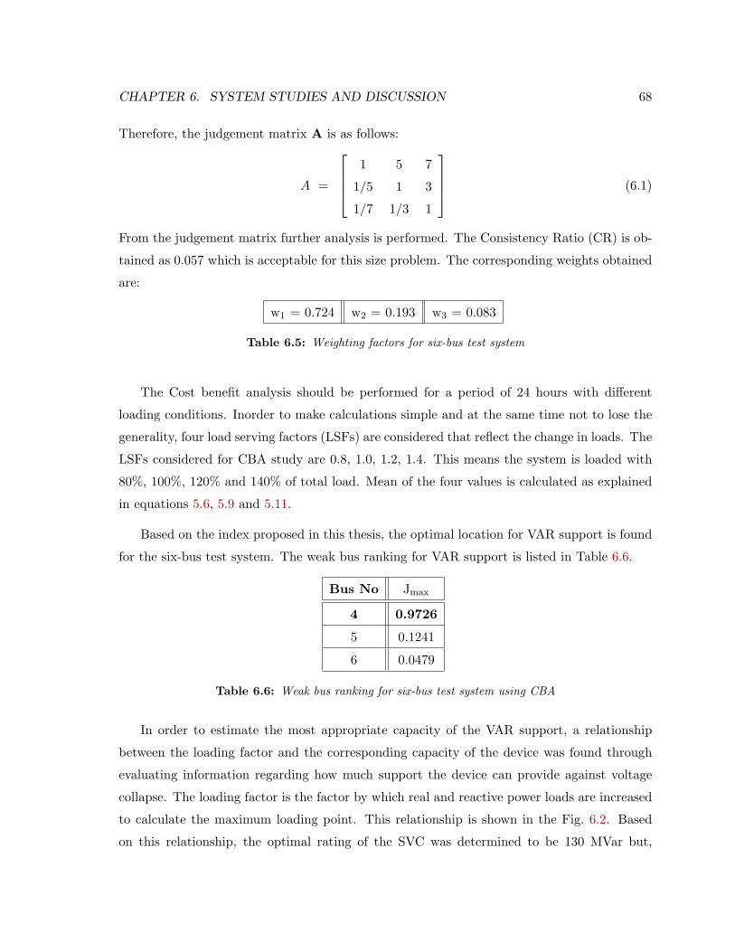
CHAPTER 6. SYSTEM STUDIES AND DISCUSSION 68
Therefore, the judgement matrix A is as follows:
A =
1 5 7
1/5 1 3
1/7 1/3 1
(6.1)
From the judgement matrix further analysis is performed. The Consistency Ratio (CR) is ob-
tained as 0.057 which is acceptable for this size problem. The corresponding weights obtained
are:
w1 = 0.724 w2 = 0.193 w3 = 0.083
Table 6.5: Weighting factors for six-bus test system
The Cost benefit analysis should be performed for a period of 24 hours with different
loading conditions. Inorder to make calculations simple and at the same time not to lose the
generality, four load serving factors (LSFs) are considered that reflect the change in loads. The
LSFs considered for CBA study are 0.8, 1.0, 1.2, 1.4. This means the system is loaded with
80%, 100%, 120% and 140% of total load. Mean of the four values is calculated as explained
in equations 5.6, 5.9 and 5.11.
Based on the index proposed in this thesis, the optimal location for VAR support is found
for the six-bus test system. The weak bus ranking for VAR support is listed in Table 6.6.
Bus No Jmax
4 0.9726
5 0.1241
6 0.0479
Table 6.6: Weak bus ranking for six-bus test system using CBA
In order to estimate the most appropriate capacity of the VAR support, a relationship
between the loading factor and the corresponding capacity of the device was found through
evaluating information regarding how much support the device can provide against voltage
collapse. The loading factor is the factor by which real and reactive power loads are increased
to calculate the maximum loading point. This relationship is shown in the Fig. 6.2. Based
on this relationship, the optimal rating of the SVC was determined to be 130 MVar but,

CHAPTER 6. SYSTEM STUDIES AND DISCUSSION 69
considering the high investment cost associated with it and keeping in mind of increase in
demand in the future, a bigger size of SVC i.e. 200MVAR is taken in this study.
0 5 10 15 20 25 30 35 400
0.1
0.2
0.3
0.4
0.5
0.6
0.7
Capacity of SVC (p.u)
Load
ing
Mar
gin
(p.u
)
Figure 6.2: Loading Margin Vs SVC Capacity for six-bus test system
Table 6.7 depicts the results of VSC-OPF with SVC for a six-bus test system. We can
observe that the system loading margin is increased and can now be loaded until 164% of its
base load.
The voltages at all buses after installing the SVC are close to the reference value which
is highly desired to restrict voltage limit violations. The three factors Social welfare, loading
capability and congestion cost benefits are given below:
Though we cannot draw any mathematical relationship between change in locational prices
with installation of SVC, but since the system loadability is being increased, the congestion
cost should decrease compared to base case. Reactive power marginal prices decreased with
the installation of SVC which is a desired incentive for new ventures.
Pricing VAR Support:
According to the pricing scheme explained in 5.28, Congestion cost decrease obtained due to
installation of SVC should be socialized or should be used for using the FACTS service.
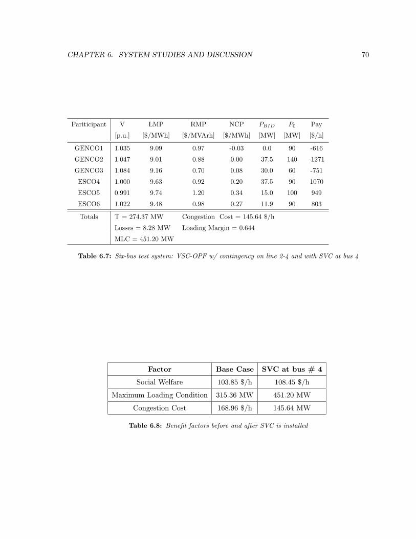
CHAPTER 6. SYSTEM STUDIES AND DISCUSSION 70
Pariticipant V LMP RMP NCP PBID P0 Pay
[p.u.] [$/MWh] [$/MVArh] [$/MWh] [MW] [MW] [$/h]
GENCO1 1.035 9.09 0.97 -0.03 0.0 90 -616
GENCO2 1.047 9.01 0.88 0.00 37.5 140 -1271
GENCO3 1.084 9.16 0.70 0.08 30.0 60 -751
ESCO4 1.000 9.63 0.92 0.20 37.5 90 1070
ESCO5 0.991 9.74 1.20 0.34 15.0 100 949
ESCO6 1.022 9.48 0.98 0.27 11.9 90 803
Totals T = 274.37 MW Congestion Cost = 145.64 $/h
Losses = 8.28 MW Loading Margin = 0.644
MLC = 451.20 MW
Table 6.7: Six-bus test system: VSC-OPF w/ contingency on line 2-4 and with SVC at bus 4
Factor Base Case SVC at bus # 4
Social Welfare 103.85 $/h 108.45 $/h
Maximum Loading Condition 315.36 MW 451.20 MW
Congestion Cost 168.96 $/h 145.64 MW
Table 6.8: Benefit factors before and after SVC is installed

CHAPTER 6. SYSTEM STUDIES AND DISCUSSION 71
1 2 3 4 5 67
7.5
8
8.5
9
9.5
10
10.5
11
11.5
12
Bus #
LMP
($/M
Wh)
Standard OPFVSC−OPF (N−1)VSC−OPF (N−1) with SVC
Figure 6.3: LMPs for the six-bus system
Therefore, from 5.29 ,
CCwof = 168.96;
CCwf = 145.64;
FP = CC|wof − CC|wf (6.2)
FP = 23.32$/h and this amount can be used to recover the investment cost of SVC.
The Fig. 6.3, Fig. 6.4, and Fig. 6.5, it is clearly shown that the marginal prices are
effected by placing VAR support. Compared to Standard OPF model, the prices obtained
through VSC-OPF are more homogeneous and decreased. The Fig. 6.6 and Fig. 6.7 shows
the effect of weighting factor p on the total transaction level ‘T’ and the maximum loading
margin λc
Observe that as expected the more the weight of loading margin, the higher the level
of security λc, but at the same time the lower the Transaction level ‘T’. This is due to the
power bids being free to vary so that, as p increases, congestion is minimized (security is
maximized) by both increasing λc and reducing ‘T’. The impact of SVC on the two factors is
quite obvious that by installing SVC the total transfer capability of the system increased there
by the system security increased. System is now stable at higher weighting factors providing

CHAPTER 6. SYSTEM STUDIES AND DISCUSSION 72
1 2 3 4 5 60.6
0.7
0.8
0.9
1
1.1
1.2
1.3
1.4
Bus #
RM
P ($
/MV
Arh
)
Standard OPFVSC−OPF (N−1)VSC−OPF (N−1) with SVC
Figure 6.4: RMPs for the six-bus system
1 2 3 4 5 6−1.5
−1
−0.5
0
0.5
1
1.5
2
2.5
3
3.5
Bus #
NC
P ($
/MW
h)
Standard OPFVSC−OPF (N−1)VSC−OPF (N−1) with SVC
Figure 6.5: NCPs for the six-bus system
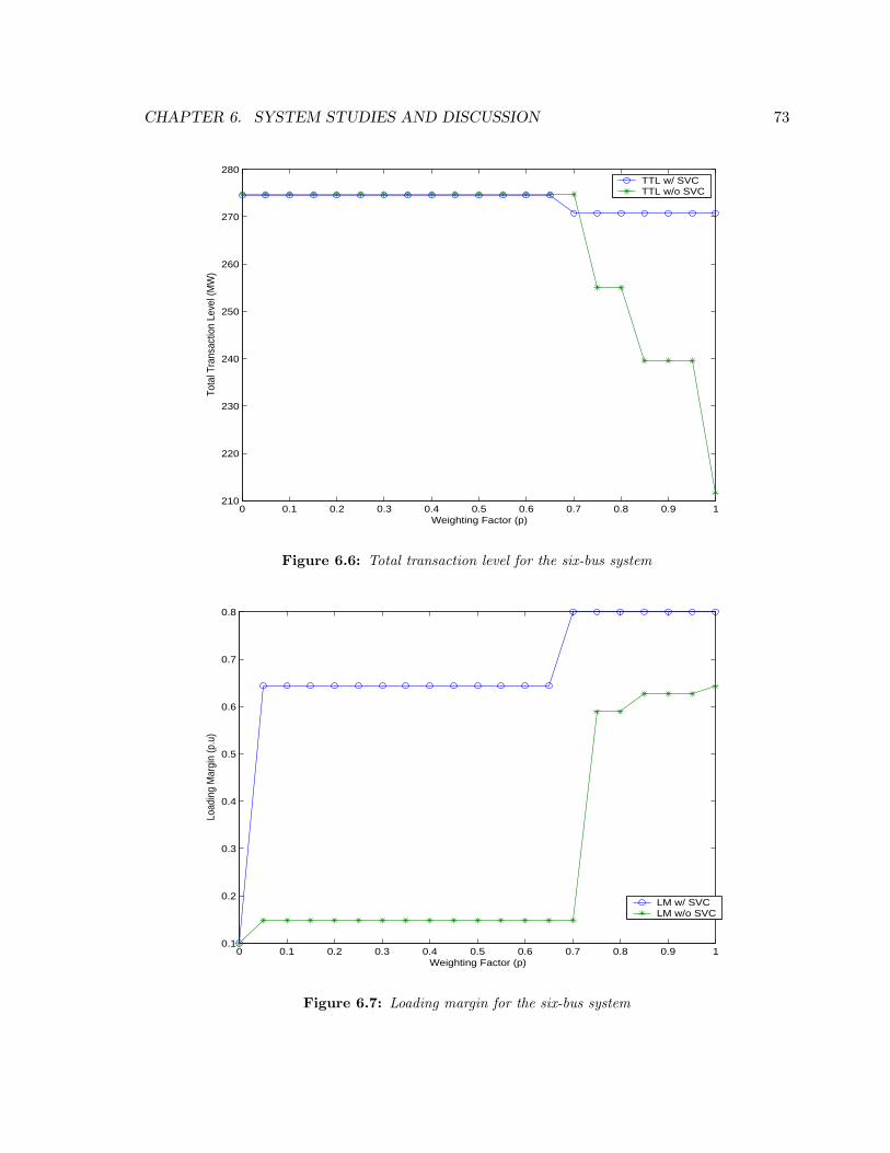
CHAPTER 6. SYSTEM STUDIES AND DISCUSSION 73
0 0.1 0.2 0.3 0.4 0.5 0.6 0.7 0.8 0.9 1210
220
230
240
250
260
270
280
Weighting Factor (p)
Tota
l Tra
nsac
tion
Leve
l (M
W)
TTL w/ SVCTTL w/o SVC
Figure 6.6: Total transaction level for the six-bus system
0 0.1 0.2 0.3 0.4 0.5 0.6 0.7 0.8 0.9 10.1
0.2
0.3
0.4
0.5
0.6
0.7
0.8
Weighting Factor (p)
Load
ing
Mar
gin
(p.u
)
LM w/ SVCLM w/o SVC
Figure 6.7: Loading margin for the six-bus system

CHAPTER 6. SYSTEM STUDIES AND DISCUSSION 74
0 0.1 0.2 0.3 0.4 0.5 0.6 0.7 0.8 0.9 1−20
0
20
40
60
80
100
120
140
160
180
Weighting Factor (p)
Con
gest
ion
Cos
t ($/
h)
CC w/ SVCCC w/o SVC
Figure 6.8: Congestion Cost for the six-bus system
constant transaction levels. In the Fig. 6.8 the impact of weighting factors on the congestion
cost is shown with and without SVC. The plot shows that the behavior of CC is same as ‘T’
as expected. At higher security, system is still able to maintain transaction levels and hence
the congestion cost exist. At lower security levels, we can observe that the congestion cost
decreased with SVC.
Fig. 6.9 depicts LMPs as p varies, illustrating the transition from an OPF market problem
to an OPF security problem as λc approaches its maximum imposed value of λcmax = 0.8.
LMPs decrease as the security levels increase, since the auction solutions move away from the
security limits (i.e., the system is less congested). Furthermore, even though the LMPs and
the overall total transaction level decrease, local bids may increase or decrease, accordingly to
the power schedule which better matches the obtained loading margin.
Wheeling Rates
The transmission prices are calculated based on wheeling charges method presented in
section 3.3. Table 6.9 gives the comparison of wheeling rates for a few selected buses with and
without SVC. The base case refers to the VSC-OPF with no critical line outage and no VAR
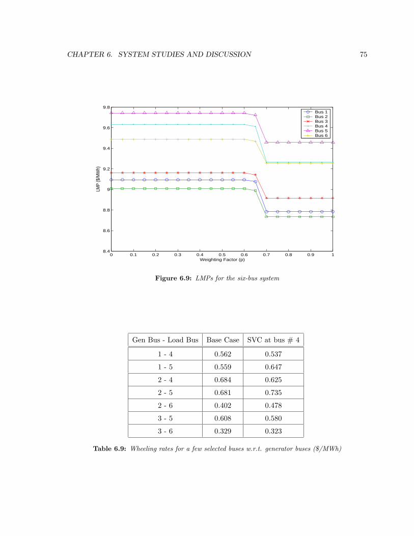
CHAPTER 6. SYSTEM STUDIES AND DISCUSSION 75
0 0.1 0.2 0.3 0.4 0.5 0.6 0.7 0.8 0.9 18.4
8.6
8.8
9
9.2
9.4
9.6
9.8
Weighting Factor (p)
LMP
($/M
Wh)
Bus 1Bus 2Bus 3Bus 4Bus 5Bus 6
Figure 6.9: LMPs for the six-bus system
Gen Bus - Load Bus Base Case SVC at bus # 4
1 - 4 0.562 0.537
1 - 5 0.559 0.647
2 - 4 0.684 0.625
2 - 5 0.681 0.735
2 - 6 0.402 0.478
3 - 5 0.608 0.580
3 - 6 0.329 0.323
Table 6.9: Wheeling rates for a few selected buses w.r.t. generator buses ($/MWh)

CHAPTER 6. SYSTEM STUDIES AND DISCUSSION 76
support. The table shows that the FACTS devices are capable to impact transmission prices.
As in the case of LMPs, the wheeling rates increase at few buses and decrease at few buses.
6.3 IEEE 14-Bus Test System
Figure 6.10: Single-line daiagram of the IEEE 14-bus test system [94]
The IEEE 14-bus test system represents a portion of the American Electric Power System
and hence can be considered a realistic example. The system has enough generation and
load to simulate an electricity market, and thus, produce significant results for examining
the algorithm and prices. The system consists of five synchronous machines two of which
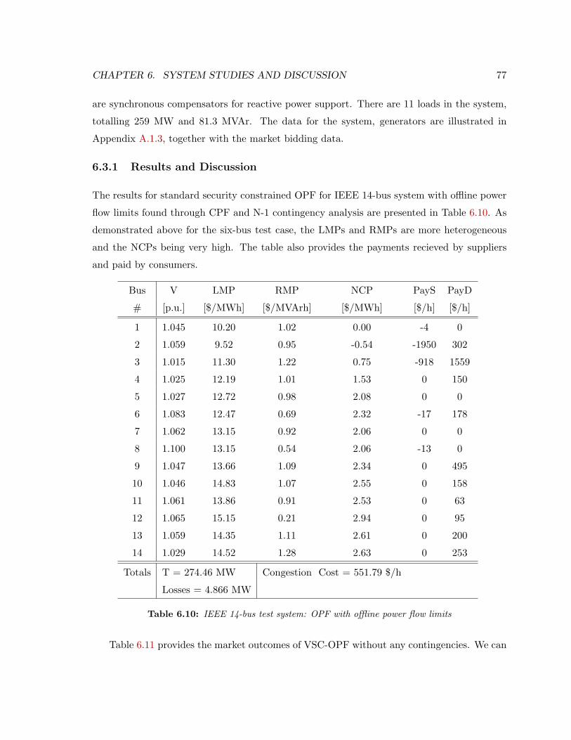
CHAPTER 6. SYSTEM STUDIES AND DISCUSSION 77
are synchronous compensators for reactive power support. There are 11 loads in the system,
totalling 259 MW and 81.3 MVAr. The data for the system, generators are illustrated in
Appendix A.1.3, together with the market bidding data.
6.3.1 Results and Discussion
The results for standard security constrained OPF for IEEE 14-bus system with offline power
flow limits found through CPF and N-1 contingency analysis are presented in Table 6.10. As
demonstrated above for the six-bus test case, the LMPs and RMPs are more heterogeneous
and the NCPs being very high. The table also provides the payments recieved by suppliers
and paid by consumers.
Bus V LMP RMP NCP PayS PayD
# [p.u.] [$/MWh] [$/MVArh] [$/MWh] [$/h] [$/h]
1 1.045 10.20 1.02 0.00 -4 0
2 1.059 9.52 0.95 -0.54 -1950 302
3 1.015 11.30 1.22 0.75 -918 1559
4 1.025 12.19 1.01 1.53 0 150
5 1.027 12.72 0.98 2.08 0 0
6 1.083 12.47 0.69 2.32 -17 178
7 1.062 13.15 0.92 2.06 0 0
8 1.100 13.15 0.54 2.06 -13 0
9 1.047 13.66 1.09 2.34 0 495
10 1.046 14.83 1.07 2.55 0 158
11 1.061 13.86 0.91 2.53 0 63
12 1.065 15.15 0.21 2.94 0 95
13 1.059 14.35 1.11 2.61 0 200
14 1.029 14.52 1.28 2.63 0 253
Totals T = 274.46 MW Congestion Cost = 551.79 $/h
Losses = 4.866 MW
Table 6.10: IEEE 14-bus test system: OPF with offline power flow limits
Table 6.11 provides the market outcomes of VSC-OPF without any contingencies. We can

CHAPTER 6. SYSTEM STUDIES AND DISCUSSION 78
observe that the LMPs and RMPs are more homogeneous. The change in LMPs resulted in
decrease of congestion cost.
Bus V LMP RMP NCP PayS PayD
# [p.u.] [$/MWh] [$/MVArh] [$/MWh] [$/h] [$/h]
1 1.100 10.20 1.02 0 -967 0
2 1.084 10.36 1.28 0.13 -2136 331
3 1.023 11.30 1.65 0.78 -998 1583
4 1.011 11.54 1.72 0.88 0 821
5 1.023 11.32 1.63 0.74 0 128
6 1.061 11.76 1.68 1.54 -40 196
7 1.040 11.82 1.83 1.36 0 0
8 1.079 11.82 1.70 1.36 -41 0
9 1.021 11.98 1.96 1.63 0 529
10 1.019 12.08 1.97 1.69 0 163
11 1.036 11.99 1.87 1.65 0 63
12 1.036 12.12 1.85 1.73 0 110
13 1.029 12.22 1.92 1.77 0 246
14 0.995 12.59 2.18 1.96 0 282
Totals T = 362.62 MW Congestion Cost = 268.94 $/h Losses = 10.753 MW
Loading Margin = 0.172 MLC = 424.97 MW
Table 6.11: IEEE 14-bus test system: VSC-OPF w/o contingencies
Table 6.12 gives the sensitivity co-efficients and the ATC values. Observe that not all the
lines that carry high powers or that have sensitivity co-efficients will be the worst outage.
Here it is evident that line 1 - 2 is the most sensitive line in the system and with the outage
of this line, the system collapses and there is no solution for VSC-OPF. This is a situation
where the installation of VAR support/SVC is desired to make the system N-1 secure and
stable. Though the system looks stable without any failure, with the critical line failure, the
system doesnt have enough resources to avoid the collapse. The optimal placement of SVC is
performed according to the algorithm proposed in 5.13
Optimal Placement of SVC:

CHAPTER 6. SYSTEM STUDIES AND DISCUSSION 79
Line # Line h− k Phk(λ) (p.u.) phk=Phk*dPhk/dλ (106) ATCN−1 (MW)
11 1-2 1.686 0.1926 -
12 3-2 0.680 0.0345 52.47
14 1-5 0.900 0.0280 49.04
15 5-4 0.566 0.0174 52.19
16 2-4 0.710 0.0074 51.27
13 3-4 0.086 0.0034 52.76
1 2-5 0.577 0.0012 51.83
4 6-13 0.273 0.0003 51.73
17 5-6 0.647 0.0002 42.55
7 9-10 0.182 0.0001 52.97
Table 6.12: IEEE 14-bus test system: Sensitivity coefficients Phk and ATC (N-1)

CHAPTER 6. SYSTEM STUDIES AND DISCUSSION 80
The approach explained in 6.2.1 for the six-bus system to find the weights for the three
BCRs is adopted for this test case. Since, the base case solution with critical line outage
has no solution the index proposed in 5.12 has been used to rank the VAR source location
sites. The tables for judgement matrix (Table 6.3) and weighting co-efficients (Table 6.13) are
illustrated again below:
A =
1 5 7
1/5 1 3
1/7 1/3 1
(6.3)
From the judgement matrix further analysis is performed. The Consistency Ratio (CR)
is obtained as 0.057 which is acceptable for this size problem. The corresponding weights
obtained are:
w1 = 0.724 w2 = 0.193 w3 = 0.083
Table 6.13: Weighting factors for IEEE 14-bus test system
The LSFs considered for this study are 0.8, 1.0, 1.2, 1.4. It means the system is loaded
with 80%, 100%, 120% and 140% of total load. Mean of the four values is calculated as
explained in equations 5.15, 5.17 and 5.19.
Based on the index explained in 5.12, the optimal location for VAR support is found for
the IEEE 14-bus test system. The weak bus ranking for VAR support is listed in Table 6.14.
From the table it is found that bus # 4 is the optimal location for VAR support where the
index J is maximum. Table 6.15 gives the single hierarchical ranking of VAR support buses
for IEEE 14-bus test system.
The single hierarchical ranking is defined as that ranking as obtained by using only one
BCR for all elements in one hierarchical structure. It can be observed from Table 6.15 that
the candidate VAR support buses selected by the three benefit-to-cost ratios (SBCR, MBCR
and CBCR) are different in ranking. Hence the need for calculating the weighting factors. In
the ranking table, it is desired that both social welfare and maximum loadability ratios to be
maximum where as the congestion cost ratio is to be minimum. Therefore, the negative sign
for CBCR in index 5.13 minimizes the congestion cost. The approach to find optimal size of

CHAPTER 6. SYSTEM STUDIES AND DISCUSSION 81
Bus No Jmax
4 0.9970
5 0.9755
9 0.9464
14 0.9387
10 0.9375
13 0.9290
11 0.9279
12 0.9241
Table 6.14: Weak bus ranking for IEEE 14-bus test system
Bus # SBCR Rank # MBCR Rank # CBCR Rank #
4 1.0000 1 1.0000 1 0.9644 6
5 0.9938 2 0.8969 2 1.0000 8
9 0.9791 4 0.8114 3 0.9762 7
10 0.9783 5 0.7745 4 0.9614 5
11 0.9729 8 0.7459 8 0.9591 4
12 0.9734 7 0.7459 7 0.9096 1
13 0.9751 6 0.7465 6 0.9516 3
14 0.9864 3 0.7605 5 0.9376 2
Table 6.15: Single hierarchical ranking of VAR support buses for IEEE 14-bus test system

CHAPTER 6. SYSTEM STUDIES AND DISCUSSION 82
SVC for this system is chosen in a similar way to six-bus test case. Fig. 6.11 depicts the plot
between loading margin and reactive power output of SVC.
0 5 10 15 20 25 30 35 400.05
0.1
0.15
0.2
0.25
0.3
0.35
0.4
0.45
0.5
Capacity of SVC (p.u)
Load
ing
Mar
gin
(p.u
)
Figure 6.11: Loading Margin Vs SVC Capacity for IEEE 14-bus test system
From the plot, it is clear that the system loading margin reaches its maximum and stables
at QSV C = 1.8p.u.. Considering the high cost involved in the investment of SVC, a device of
capacity 2.5 p.u. is taken in this study for this system. Table 6.16 illustrates the spot prices
and the benefits obtained by installing SVC at the optimal location. Also observe that the
bus voltages in the three cases, the system with SVC at bus # 4 has got the voltages close to
1.0 which is desired at higher loading levels inorder to avoid voltage collapses.
The system which was prone to collapse and failed to maintain minimum level of security
with the critical line outage is now able to withstand the failure of line with the installation
of VAR support. The system with SVC is stable in all aspects. The congestion cost decreased
compared to standard OPF where as losses are increased which is expected because of the
increase in the transaction level. The loading margin which is less then 0.1 with no SVC
has been increased to 0.475 i.e. the system can be loaded safely upto 140% of base load by
maintaining minimum level of security.
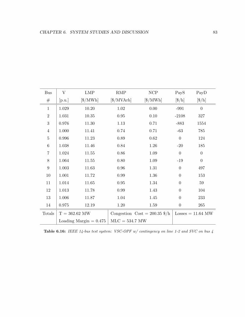
CHAPTER 6. SYSTEM STUDIES AND DISCUSSION 83
Bus V LMP RMP NCP PayS PayD
# [p.u.] [$/MWh] [$/MVArh] [$/MWh] [$/h] [$/h]
1 1.029 10.20 1.02 0.00 -991 0
2 1.031 10.35 0.95 0.10 -2108 327
3 0.976 11.30 1.13 0.71 -883 1554
4 1.000 11.41 0.74 0.71 -63 785
5 0.996 11.23 0.89 0.62 0 124
6 1.038 11.46 0.84 1.26 -20 185
7 1.024 11.55 0.86 1.09 0 0
8 1.064 11.55 0.80 1.09 -19 0
9 1.003 11.63 0.96 1.31 0 497
10 1.001 11.72 0.99 1.36 0 153
11 1.014 11.65 0.95 1.34 0 59
12 1.013 11.78 0.99 1.43 0 104
13 1.006 11.87 1.04 1.45 0 233
14 0.975 12.19 1.20 1.59 0 265
Totals T = 362.62 MW Congestion Cost = 200.35 $/h Losses = 11.64 MW
Loading Margin = 0.475 MLC = 534.7 MW
Table 6.16: IEEE 14-bus test system: VSC-OPF w/ contingency on line 1-2 and SVC on bus 4
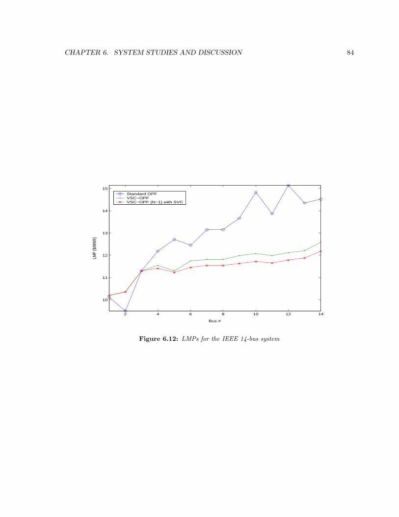
CHAPTER 6. SYSTEM STUDIES AND DISCUSSION 84
2 4 6 8 10 12 14
10
11
12
13
14
15
Bus #
LMP
($/M
Wh)
Standard OPFVSC−OPFVSC−OPF (N−1) with SVC
Figure 6.12: LMPs for the IEEE 14-bus system

CHAPTER 6. SYSTEM STUDIES AND DISCUSSION 85
2 4 6 8 10 12 14
0.4
0.6
0.8
1
1.2
1.4
1.6
1.8
2
Bus #
RM
P ($
/MV
Arh
)
Standard OPFVSC−OPFVSC−OPF (N−1) with SVC
Figure 6.13: RMPs for the IEEE 14-bus system
From Fig. 6.12 depicts the LMPs at all the buses. We can observe that the LMPs decreased
with the case without any contingency. Observe that the LMPs obtained for standard OPF
with offline power flow limits are heterogeneous and very high compared to the other two
cases. The improvement in the LMPs and change in power bids help to decrease congestion
cost and to increase transaction levels.
The reactive power marginal prices in Fig. 6.13 obtained by placing SVC are more homo-
geneous and are lesser compared to standard OPF and with VSC-OPF with no contingency.
The loads are required to maintain a constant power factor of 0.92 and this high power factor
leads to lower RMPs. Observe that from Fig. 6.14 the nodal congestion prices (NCPs) reduced
compared to both standard OPF and voltage stability OPF.
Wheeling Rates The wheeling charges calculated for few selected load buses w.r.t generator
buses are shown in Table 6.17. The base case refers to the VSC-OPF with no contingencies
as the system with critical line outage is not stable. It is evident that the wheeling charges
decreased for the case with SVC at bus # 4 compared to the one with no SVC.
Analysis of Reactive Power Pricing

CHAPTER 6. SYSTEM STUDIES AND DISCUSSION 86
2 4 6 8 10 12 14−0.5
0
0.5
1
1.5
2
2.5
Bus #
NC
P ($
/MW
h)Standard OPFVSC−OPFVSC−OPF (N−1) with SVC
Figure 6.14: NCPs for the IEEE 14-bus system
Gen Bus - Load Bus Base Case SVC at bus # 4
1 - 5 1.115 1.031
2 - 4 1.182 1.058
2 - 5 0.954 0.879
3 - 4 0.243 0.109
6 - 11 0.230 0.193
6 - 12 0.360 0.322
6 - 13 0.462 0.415
Table 6.17: Wheeling rates for a few selected buses w.r.t. generator buses ($/MWh)

CHAPTER 6. SYSTEM STUDIES AND DISCUSSION 87
0.7 0.75 0.8 0.85 0.9 0.95 10
0.2
0.4
0.6
0.8
1
1.2
1.4
1.6
1.8
2
Power Factor
Rea
ctiv
e P
ower
Mar
gina
l Pric
e ($
/MV
Arh
)
Bus 2Bus 3Bus 5Bus 6Bus 7Bus 8Bus 9Bus 10Bus 11Bus 12Bus 13Bus14
Figure 6.15: RMPs for the IEEE 14-bus system
In this case, the impact of load power factor on RMP is studied. From Fig. 6.15, 6.16,
6.17 we can see:
1. When the load power factor reduces from 1.0 to 0.7, the RMP increases gradually.
Therefore, the RMP can provide clear economic information to loads to improve their
power factors.
2. In Fig. 6.16 when the power factor is close to 1, the reactive power output of the two
generators becomes negative. This means that the system has surplus reactive power
and the generators are asked to absorb excessive reactive power. The corresponding
RMPs in 6.15 are also low or at their minimum.
3. When the voltage of bus 3 reduced with the decrease in power factor, the corresponding
RMP increased rapidly.
4. The revenue of reactive power supply based on the marginal price will be much more
than that based on the average price especially at lower power factors. Therefore some
adjustment should be made if RMP is going to be used.

CHAPTER 6. SYSTEM STUDIES AND DISCUSSION 88
0.7 0.75 0.8 0.85 0.9 0.95 1−50
0
50
100
150
200
250
Power Factor
Rea
ctiv
e P
ower
Out
puts
(MW
)
Bus 1Bus 2Bus 3Bus 4Bus 6Bus 8
Figure 6.16: Reactive Power output of generators for IEEE 14-bus system
0.7 0.75 0.8 0.85 0.9 0.95 10.9
0.95
1
1.05
1.1
1.15
Power Factor
Bus
Vol
tage
s
Bus 2Bus 3Bus 5Bus 6Bus 7Bus 8Bus 9Bus 10Bus 11Bus 12Bus 13Bus14
Figure 6.17: Bus Voltages for IEEE 14-bus system

CHAPTER 6. SYSTEM STUDIES AND DISCUSSION 89
6.4 Summary
The impact of VAR support on the electricity market prices is studied. Electricity market is
designed as a multi-objective OPF problem that maximizes social welfare and loading margin.
The index to identify and rank candidate VAR source nodes is tested on a six-bus and a
realistic IEEE 14-bus test system.

Chapter
7
Conclusions and Future Work
7.1 Principal Contributions
An approach to study the impact of optimally placed VAR support on electrity spot pricing in
the deregulated electricity market is proposed. The multi-objective OPF is modified to include
the reactive power production and consumption costs which provides proper market signals
to restrict the reactive power usage and maintain good power factor. An index to place VAR
support such that the social welfare, maximum loading condition are improved and congestion
costs are reduced based on a cost benefit analysis is proposed. Analytic Hierarchy Process
which can be used to find weights for different terms which are not related qualitatively is
extended to use in the complicated power systems to find appropriate weighting factors for
different benefit-to-cost ratios but based on engineers knowledge of each of these terms.
This thesis has described a new approach of transmission pricing calculation taking VSC-
OPF based multi-objective maximization as the objective and has studied the impact of
FACTS devices on it. A simple method to price VAR support such that the investment cost is
recovered from the market solution is proposed according to congestion cost of the system. An
analysis of reactive power pricing is performed such that the RMPs can provide clear economic
information to loads to improve their power factors.
90

CHAPTER 7. CONCLUSIONS AND FUTURE WORK 91
7.2 Possible Future Directions
Some possible future directions for this work are:
1. The loads considered in this study are elastic, i.e. price sensitive. Studies with voltage
dependent loads may help to better understand the impact of load voltages on market
solutions.
2. Real market scenario can be replicated by the multi-agent systems. GENCOs, TRANSCOs
DISCOs and ESCOs can all be different agents that communicate each other in real time
operations.
3. The principal’s of optimal location in transmission system can be extended to distribu-
tion system with the help of GIS.

Appendix
A
APPENDIX A
A.1 Network and Market Data
A.1.1 PSAT Data Format
The following tables 1 illustrate the PSAT data structure.
Table A.1: Bus Data Format (Bus.con)
Column Description Unit1 Bus number int2 Voltage base kV†3 Voltage amplitude initial guess p.u.†4 Voltage phase initial guess rad†5 Area number (not used yet...) int†6 Region number (not used yet...) int
1In this table and remaining tables in this chapter, fields marked with † are optional
92

APPENDIX A. APPENDIX A 93
Table A.2: PQ Data Format (PQ.con)
Column Description Unit1 Bus number int2 Power rating MVA3 Voltage rating kV4 Active power p.u.5 Reactive power p.u.† 6 Maximum voltage p.u.† 7 Minimum voltage p.u.† 8 Allow conversion to impedance boolean.
Table A.3: PV Data Format (PV.con)
Column Description Unit1 Bus number int2 Power rating MVA3 Voltage rating kV4 Active power p.u.5 Voltage magnitude p.u.† 6 Maximum reactive power p.u.† 7 Minimum reactive power p.u.† 8 Maximum voltage p.u.† 9 Minimum voltage p.u.†10 Loss participation coefficient −
Table A.4: Shunt Data Format (Shunt.con)
Column Description Unit1 Bus number int2 Power rating MVA3 Voltage rating kV4 Frequency rating Hz5 Conductance p.u.6 Susceptance p.u.

APPENDIX A. APPENDIX A 94
Table A.5: SW Data Format (SW.con)
Column Description Unit1 Bus number int2 Power rating MVA3 Voltage rating kV4 Voltage magnitude p.u.5 Reference angle p.u.† 6 Maximum reactive power p.u.† 7 Minimum reactive power p.u.† 8 Maximum voltage p.u.† 9 Minimum voltage p.u.†10 Active power guess p.u.†11 Loss participation coefficient −
Table A.6: Line Data Format (Line.con)
Column Description Unit1 From Bus int2 To Bus int3 Power Rating MVA4 Voltage Rating kV5 Frequency Rating Hz6 Line Length km7 (not used yet...) −8 Resistance p.u. (Ω / km )9 Reactance p.u. ( H / km )10 Susceptance p.u. ( F / km )† 11 (not used yet...) −† 12 (not used yet...) −† 13 Current limit p.u.† 14 Active power limit p.u.† 15 Apparent power limit p.u.
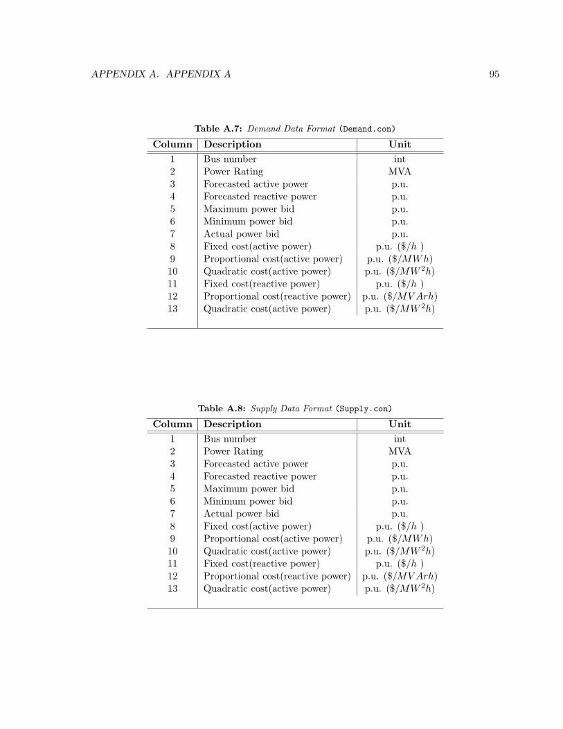
APPENDIX A. APPENDIX A 95
Table A.7: Demand Data Format (Demand.con)
Column Description Unit1 Bus number int2 Power Rating MVA3 Forecasted active power p.u.4 Forecasted reactive power p.u.5 Maximum power bid p.u.6 Minimum power bid p.u.7 Actual power bid p.u.8 Fixed cost(active power) p.u. ($/h )9 Proportional cost(active power) p.u. ($/MWh)10 Quadratic cost(active power) p.u. ($/MW 2h)11 Fixed cost(reactive power) p.u. ($/h )12 Proportional cost(reactive power) p.u. ($/MV Arh)13 Quadratic cost(active power) p.u. ($/MW 2h)
Table A.8: Supply Data Format (Supply.con)
Column Description Unit1 Bus number int2 Power Rating MVA3 Forecasted active power p.u.4 Forecasted reactive power p.u.5 Maximum power bid p.u.6 Minimum power bid p.u.7 Actual power bid p.u.8 Fixed cost(active power) p.u. ($/h )9 Proportional cost(active power) p.u. ($/MWh)10 Quadratic cost(active power) p.u. ($/MW 2h)11 Fixed cost(reactive power) p.u. ($/h )12 Proportional cost(reactive power) p.u. ($/MV Arh)13 Quadratic cost(active power) p.u. ($/MW 2h)

APPENDIX A. APPENDIX A 96
A.1.2 6-Bus Test System
Bus.con = [ ...
1 400 1 0 2 1;
2 400 1 0 2 1;
3 400 1 0 2 1;
4 400 1 0 2 1;
5 400 1 0 2 1;
6 400 1 0 2 1 ];
Line.con = [ ...
2 3 100 400 60 0 0 0.05 0.25 0.06 0 0 1.3856 0.1827;
3 6 100 400 60 0 0 0.02 0.1 0.02 0 0 1.3856 0.4745;
4 5 100 400 60 0 0 0.2 0.4 0.08 0 0 1.3856 0.0773;
3 5 100 400 60 0 0 0.12 0.26 0.05 0 0 1.3856 0.2304;
5 6 100 400 60 0 0 0.1 0.3 0.06 0 0 1.3856 0.0219;
2 4 100 400 60 0 0 0.05 0.1 0.02 0 0 1.3856 0.5769;
1 2 100 400 60 0 0 0.1 0.2 0.04 0 0 1.3856 0.1174;
1 4 100 400 60 0 0 0.05 0.2 0.04 0 0 1.3856 0.3984;
1 5 100 400 60 0 0 0.08 0.3 0.06 0 0 1.3856 0.5044;
2 6 100 400 60 0 0 0.07 0.2 0.05 0 0 1.3856 0.4332;
2 5 100 400 60 0 0 0.1 0.3 0.04 0 0 1.3856 0.3311];
SW.con = [ ...
2 100 400 1.05 0 1.5 -0.15 1.1 0.9 1.03 1 ];
PV.con = [ ...
1 100 400 0.675 1.05 1.5 -0.15 1.1 0.9 1;
3 100 400 0.45 1.05 1.5 -0.15 1.1 0.9 1];
PQ.con = [ ...
4 100 400 0.675 0.45 1.1 0.9 0;
5 100 400 0.75 0.525 1.1 0.9 0;
6 100 400 0.675 0.45 1.1 0.9 0 ];
Demand.con = [ ...
4 100 0.25 0.1210 0.375 1e-5 0 0 12 0 0 1.20 0 1;
5 100 0.1 0.0484 0.15 1e-5 0 0 10.5 0 0 1.05 0 1;
6 100 0.2 0.0968 0.3 1e-5 0 0 9.5 0 0 0.95 0 1 ];
Supply.con = [ ...
1 100 0.3 0.3 1e-005 0 0 9.7 0 0 0.97 0 0 0;
2 100 0.375 0.375 1e-005 0 0 8.8 0 0 0.88 0 0 0;
3 100 0.3 0.3 1e-005 0 0 7 0 0 0.70 0 0 0];
Varname.bus = ...
’Bus1’; ’Bus2’; ’Bus3’; ’Bus4’; ’Bus5’;
’Bus6’;
Bus.con(:,3) = [...
1.0500000; 1.0500000; 1.0500000; 1.0048; 0.99391;
1.0086];
Bus.con(:,4) = [...
0.01895; 0.0000000;-0.02549;-0.03039;-0.05393;
-0.05415];
A.1.3 IEEE 14-Bus Test System
Bus.con = [ ...

APPENDIX A. APPENDIX A 97
1 69 1 0 4 1;
2 69 1 0 4 1;
3 69 1 0 4 1;
4 69 1 0 4 1;
5 69 1 0 4 1;
6 13.8 1 0 2 1;
7 13.8 1 0 2 1;
8 18 1 0 3 1;
9 13.8 1 0 2 1;
10 13.8 1 0 2 1;
11 13.8 1 0 2 1;
12 13.8 1 0 2 1;
13 13.8 1 0 2 1;
14 13.8 1 0 2 1 ];
Line.con = [ ...
2 5 100 69 60 0 0 0.05695 0.17388 0.034 0 0 0 0 0;
6 12 100 13.8 60 0 0 0.12291 0.25581 0 0 0 0 0 0;
12 13 100 13.8 60 0 0 0.22092 0.19988 0 0 0 0 0 0;
6 13 100 13.8 60 0 0 0.06615 0.13027 0 0 0 0 0 0;
6 11 100 13.8 60 0 0 0.09498 0.1989 0 0 0 0 0 0;
11 10 100 13.8 60 0 0 0.08205 0.19207 0 0 0 0 0 0;
9 10 100 13.8 60 0 0 0.03181 0.0845 0 0 0 0 0 0;
9 14 100 13.8 60 0 0 0.12711 0.27038 0 0 0 0 0 0;
14 13 100 13.8 60 0 0 0.17093 0.34802 0 0 0 0 0 0;
7 9 100 13.8 60 0 0 0 0.11001 0 0 0 0 0 0;
1 2 100 69 60 0 0 0.01938 0.05917 0.0528 0 0 0 0 0;
3 2 100 69 60 0 0 0.04699 0.19797 0.0438 0 0 0 0 0;
3 4 100 69 60 0 0 0.06701 0.17103 0.0346 0 0 0 0 0;
1 5 100 69 60 0 0 0.05403 0.22304 0.0492 0 0 0 0 0;
5 4 100 69 60 0 0 0.01335 0.04211 0.0128 0 0 0 0 0;
2 4 100 69 60 0 0 0.05811 0.17632 0.0374 0 0 0 0 0;
5 6 100 69 60 0 5 0 0.25202 0 0.932 0 0 0 0;
4 9 100 69 60 0 5 0 0.55618 0 0.969 0 0 0 0;
4 7 100 69 60 0 5 0 0.20912 0 0.978 0 0 0 0;
8 7 100 18 60 0 1.30435 0 0.17615 0 0 0 0 0 0 ];
Line.con(:,13) = 1.5498;
Line.con(:,14) = [0.49535; 0.09027; 0.01987; 0.21251; 0.08948; 0.03882; 0.07662; 0.12167; 0.07268; 0.38089;...
1.9237; 0.89421; 0.24213; 0.89121; 0.78599; 0.6519; 0.54778; 0.21166; 0.38089; 0]*0.9;
SW.con = [ ...
1 100 69 1.06 0 1.0 -0.4 1.1 0.9 2.324 1 ];
PV.con = [ ...
2 100 69 0.4 1.045 0.5 -0.4 1.1 0.9 1;
3 100 13.8 0 1.07 0.4 -0.4 1.1 0.9 1;
6 100 69 0 1.01 0.24 -0.06 1.1 0.9 1;
8 100 18 0 1.09 0.24 -0.06 1.1 0.9 1 ];
PQ.con = [ ...
11 100 13.8 0.035 0.018 1.1 0.9 0;
13 100 13.8 0.135 0.058 1.1 0.9 0;
3 100 69 0.942 0.19 1.1 0.9 0;
5 100 69 0.076 0.016 1.1 0.9 0;
2 100 69 0.217 0.127 1.1 0.9 0;
6 100 13.8 0.112 0.075 1.1 0.9 0;
4 100 69 0.478 0.04 1.1 0.9 0;
14 100 13.8 0.149 0.05 1.1 0.9 0;
12 100 13.8 0.061 0.016 1.1 0.9 0;
10 100 13.8 0.09 0.058 1.1 0.9 0;
9 100 13.8 0.295 0.166 1.1 0.9 0 ];

APPENDIX A. APPENDIX A 98
Supply.con = [ ...
1 100 0.10 1.0 1e-005 0 0 10.2 0 0 1.02 0 0 0;
2 100 0.10 2.0 1e-005 0 0 9.5 0 0 0.95 0 0 0;
3 100 0.10 2.0 1e-005 0 0 11.3 0 0 1.13 0 0 0];
Demand.con = [ ...
2 100 0.1519 0.0646 0.3038 1e-5 0 0 13 0 0 1.300 0 0 0;
3 100 0.6595 0.2803 1.319 1e-5 0 0 13.2 0 0 1.320 0 0 0;
4 100 0.3346 0.1422 0.6692 1e-5 0 0 12.1 0 0 1.210 0 0 0;
5 100 0.0532 0.0226 0.1064 1e-5 0 0 12.33 0 0 1.233 0 0 0;
6 100 0.0784 0.0333 0.1568 1e-5 0 0 12.24 0 0 1.224 0 0 0;
9 100 0.2065 0.0878 0.4130 1e-5 0 0 13.55 0 0 1.355 0 0 0;
10 100 0.063 0.0268 0.1260 1e-5 0 0 14.66 0 0 1.466 0 0 0;
11 100 0.0245 0.0104 0.0490 1e-5 0 0 13.67 0 0 1.367 0 0 0;
12 100 0.0427 0.0182 0.0854 1e-5 0 0 14.62 0 0 1.462 0 0 0;
13 100 0.0945 0.0402 0.1890 1e-5 0 0 14.22 0 0 1.422 0 0 0;
14 100 0.1043 0.0443 0.2086 1e-5 0 0 14.45 0 0 1.445 0 0 0];
Demand.con(:,4) = Demand.con(:,3)*0.425;
Varname.bus = ...
’Bus 01’; ’Bus 02’; ’Bus 03’; ’Bus 04’; ’Bus 05’;
’Bus 06’; ’Bus 07’; ’Bus 08’; ’Bus 09’; ’Bus 10’;
’Bus 11’; ’Bus 12’; ’Bus 13’; ’Bus 14’;

References
[1] Abdel-Moamen, M. A., Padhy, N. P., “Optimal power flow incorporating FACTS devices- bibliography and survey,” IEEE PES Transmission and Distribution Conference andExposition, Vol. 2, pp. 669-676, Sept. 2003.
[2] Ajjarapu, V., Christy, C., “The Continuation Power Flow: A Tool for Steady StateVoltage Stability Analysis,” IEEE Transactions on Power Systems, Vol. 7, no. 1, pp.416-423, Feb. 1992.
[3] Alsac, O., Bright, J., Prais, M., Stott, M., “Further Developments in LP based OptimalPower Flow, ” IEEE Transactions on Power Systems, Vol. 5, no. 3, pp. 697-711, Aug.1990.
[4] Alvarado, F. L., Jung, T. H., “Direct Detection of Voltage Collapse Conditions,” Proc.Bulk Power System Voltage Phenomena-Voltage Stability and Security , EL-6183, EPRI,pp. 5.23-5.38, Jan. 1989.
[5] Ambriz-Perez, H., Acha, E., Fuerte-Esquivel, C. R., “Advanced SVC models for Newton-Raphson load flow and Newton optimal power flow studies,” IEEE Transactions onPower Systems, Vol. 15, no. 1, pp. 129-136, Feb. 2000.
[6] Ambriz-Perez, H. et al., “Incorporation of a UPFC model in an optimal power flow usingNewton’s method,” IEE Proceedings: Generation, Transmission and Distribution, Vol.145, no. 3, pp. 336-344, May 1998.
[7] Arabi, S., Kundur, P., Adapa, R., “Innovative Techniques in Modeling UPFC for PowerSystem Analysis,” IEEE Transactions of Power Systems, Vol. 15, No. 1, pp. 336-341,Feb. 2000.
[8] Available Transfer Capability Definition and Determination, Tech. rep., NERC, USA(1996).
99

REFERENCES 100
[9] Barcelo, W. R., Lemmon, W. W., “Standardized Sensitivity Coeffcients for Power Sys-tem Networks,” IEEE Transactions on Power Systems, Vol. 3, no. 4, pp. 1591-1599,Nov. 1988.
[10] Baughman, M. L., Siddiqi, S. N., “Real Time Pricing of Reactive Power: Theory andCase Study Results,” IEEE Transactions on Power Systems, Vol. 6, no. 1, pp. 23-29,Feb. 1993.
[11] Berizzi, A. et al., “Enhanced Security-Constrained OPF With FACTS Devices,” IEEETransactions on Power Systems, Vol. 20, no. 3, pp. 1597-1605, Aug. 2005.
[12] Brooke, A., Kendrick, D., Meeraus, A., Raman, R., Rosenthal, R. E., GAMS, a User’sGuide, available at http://www.gams.com/.
[13] Cai, L. J., Erlich, I., Stamtsis, G. C., “Optimal choice and allocation of FACTS devicesusing genetic algorithms,” IEEE PES Power Systems Conference and Exposition, Vol.1, pp. 201-207, 2004.
[14] Californina Power Market, Online: http://www.caiso.com/.[15] Canizares, C. A., Alvarado, F. L., “Point of Collapse and Continuation Methods for
Large AC/DC Systems,” IEEE Transactions on Power Systems, Vol. 8, no. 1, pp. 1-8,Feb. 1993.
[16] Canizares, C. A., “Applications of Optimization to Voltage Collapse Analysis,” IEEE-PES Summer Meeting, San Diego, USA, July 1998.
[17] Canizares, C. A., Faur, Z. T., “Analysis of SVC and TCSC controllers in voltage col-lapse,” IEEE Transactions on Power Systems,Vol. 14, no. 1, pp. 158-165, Feb. 1999.
[18] Canizares, C. A., Rosehart, W., Quintana, V. H., “Costs of Voltage Security in Electric-ity Markets,” Proc. 2001 IEEE-PES Summer Meeting, Seattle, WA, USA, July 2000.
[19] Canizares, C. A., Chen, H., Rosehart, W., “Pricing System Security in Electricity Mar-kets,” Proceedings Bulk Power systems Dynamics and Control - V, Onomichi, Japan,September 2001.
[20] Canizares, C. A., “Voltage Stability Assesment : Concepts Practices and Tools,” IEEE-PES Power System Stability Subcommittee Special Publication, SP101PSS, TechnicalReport, 2002.
[21] Canizares, C. A., Kodsi, S. K. M., “Dynamic versus steady-state modeling of FACTScontrollers in transmission congestion,” IEEE Power Engineering Society General Meet-ing, June 2006.
[22] Carpentier, J., “Contribution a l’etude du Dispatch Economique,” Bulletin de la Societe.Francaise des Electriciena, Series. 8, Vol. 3, August 1962.
[23] Cazzol, M. V. et al., “Unified power flow controller (UPFC) model in the frameworkof interior point based active and reactive OPF procedure,” International Journal ofElectrical Power and Energy Systems, Vol. 24, no. 6, pp. 431-437, August 2002.
[24] Chattopadhyay, D., Bhattacharya, K., Parikh, J., “Optimal reactive power planning andits spot-pricing: an integrated approach,” IEEE Transactions on Power Systems, Vol.10, no. 4, pp. 2014-2020, Nov. 1995.

REFERENCES 101
[25] Chiang, H. D., Flueck, A. J., Shah, K. S., Balu, N., “CPFLOW: A Pratical Tool forTracing Power System Steady-State Stationary Behavior Due to Load and GenerationVariations,” IEEE Transactions on Power Systems, Vol. 10, no. 2, pp. 623-634, May1995.
[26] Chen, A. H. L., Nwankpa, C. O., Kawatny, H. G. and ming Yu, X., “ Voltage StabilityToolbox: An Introduction and Implementation, ” Proceedings of North American PowerSymposium, MIT, 1996.
[27] Choi, J. Y., Rim, S. H., Park, J. K., “Optimal real time pricing of real and reactivepowers,” IEEE Transactions on Power Systems, Vol. 3, no. 4, pp. 1226-1231, Nov. 1998.
[28] Chow, J., “Power System Toolbox Version 2.0: Load Flow Tutorial and Functions,”Cherry Tree Scientific Software, RR-5 Colborne, Ontario K0K 1S0, 1991-1999.
[29] Chung, T. S., Li, Y. Z.,“A hybrid GA approach for OPF with consideration of FACTSdevices,” IEEE Power Engineering Review, Vol. 21, no. 2, pp. 47-50, Feb. 2001.
[30] De Souza, A. C. Z., Canizares, C.A., Quintana, V. H., “New techniques to speed upvoltage collapse computations using tangent vectors,” IEEE Transactions on PowerSystems, Vol. 12, No. 3, pp. 1380-1387, Aug. 1997.
[31] Einbom, M., Siddiqi, R., “Electricity Transmission Pricing and Technology,” KluwerAcademic Publisher, Boston, MA, 1996.
[32] El-Keib, A. A., Ma, X., “Calculating of Short-run Marginal Costs of Active and ReactivePower Production,” IEEE Transactions on Power Systems, Vol. 12, no. 1, pp. 559-565,May 1997.
[33] Feng, W., Shrestha, G. B.,“Allocation of TCSC devices to optimize total transmissioncapacity in a competitive power market,” Proceedings of the IEEE Power EngineeringSociety Transmission and Distribution Conference, Vol. 2, pp. 587-593, 2001.
[34] Feng, W., Shrestha, G. B.,“ Impacts of TCPAR on spot price power markets,” Proceed-ings of Fifth International Power Engineering Conference (IPEC 2001), Vol. 2, Pt. 2,pp. 592-597, May 2001.
[35] Galiana, G. D., “Assessment and Control of the Impact of FACTS devices on PowerSystem Performance,” IEEE Transactions on Power Systems, Vol. 11, No. 4, pp. 1931-1936, November 1996.
[36] Gerbex, S., Cherkaoui, R., Germond, A. J., “Optimal location of multi-type FACTSdevices in a power system by means of genetic algorithms,” IEEE Transactions onPower Systems, Vol. 16, no. 3, pp.537-544, Aug. 2001.
[37] Gyugyi, L., “Power Electronics in Electrical Utilitis: Static Var Compensators,” Pro-ceedings of the IEEE, Vol. 76 No. 4, pp.483-494, April. 1988.
[38] Gyugi, L. et al., “The Unified power flow controller: a new approach to power trans-mission control,” IEEE Transactions on Power Delivery, Vol. 10, no. 2, pp. 1085-1093,April 1995.
[39] Habur, K., and Oleary, D., “FACTS - Flexiable Alternating Current Transmission Sys-tems, For cost effective and reliable transmission of electrical energy,” Available Online: http://www.siemenstd.com/TransSys/pdf/CostEffectiveReliabTrans.pdf.
REFERENCES 102
[40] Hammons, T. J., Lim, S. K., “Flexible AC Transmission System(FACTS),” ElectricMachines and Power Systems, Vol. 25, pp. 73-85, 1997.
[41] Hao, S., Papalexopoulos, A., “Reactive Power Pricing and Management,” IEEE Trans-actions on Power Systems, Vol. 12, no. 1, pp. 95-104, Feb. 1997.
[42] Hasanovic, A., “Modelling and Control of Unified Power Flow Controller (UPFC), thesis,West Virginia University, 2000.
[43] Hingorani, N. G., “Power Electronics in Electrical utilities: Rule of Power Electronicsin Future Power Systems,” Proceedings of the IEEE, Vol. 76, No. 4, pp.481-482, April1988.
[44] Hingorani, N. G., “High Power Electronics and Flexible AC Transmission System,”IEEE Power Engineering Review, NO. 7, pp 3-4, July 1988.
[45] Hingorani, N. G., Gyugyi, L., “Understanding FACTS Concepts and Technology ofFlexible AC Transmission System,” IEEE Press, 2000.
[46] Huang,G. M., Yan, P., “TCSC and SVC as Re-dispatch Tools for Congestion Man-agement and TTC Improvement,” Proceedings of the IEEE Power Engineering SocietyTransmission and Distribution Conference, Vol. 1, pp. 660-665, 2002.
[47] Huang,G. M., Yan, P., “Establishing Pricing Schemes for FACTS Devices in CongestionManagement,” IEEE PES General Meeting, Vol.2, No.2, pp. 1025-30, July 2003.
[48] Huneault, M., Galiana, F. D., “A Survey of the Optimal Power Flow Literature,” IEEETransactions on Power Systems, Vol. 6, no. 2, pp. 762-770, May 1991.
[49] Irisarri, G, D., Wang, X., Tong, J., Mokhtari, S., “Maximum Loadability of PowerSystems using Interior Point Nonlinear Optimization Method,” IEEE Transactions onPower Systems, Vol. 12, no. 1, pp. 162-172, Feb. 1997.
[50] Kodsi, S. K. M., Accounting for the Effects of Power System Controllers and Stabilityon Power Dispatch and Electricity Market Prices, dissertation, University of Waterloo,Ontario, Canada, 2005.
[51] Kundur, P., “Power System Stability and Control,” McGraw-Hill, 1994.[52] Kundur, P., Paserba, J., Ajjarappu, V., et.al, “Definition and classification of power
system stability IEEE/CIGRE joint task force on stability terms and definitions,” IEEETransactions on Power Systems, Vol. 19, no. 3, pp. 1387-1401, Aug. 2004.
[53] Lakkaraju, T., Feliachi, A., “Selection of Pilot buses for VAR Support Considering N-1Contingency Criteria,” IEEE Power Systems Conference and Exposition, Nov 2006.
[54] Lamont, J. W., Fu. J., “Cost Analysis of Reactive Power Support,” IEEE Transactionson Power Systems, Vol. 14, no. 3, pp. 890-898, Aug. 1999
[55] Leung, H. C., Chung, T. S., “Optimal placement of FACTS controller in power systemby a genetic-based algorithm,” Proceedings of the IEEE 1999 International Conferenceon Power Electronics and Drive Systems. PEDS’99, Vol. 2, Pt. 2, pp. 833-836, 1999.
[56] Leung, H. C., Chung, T. S., “Optimal power flow with a versatile FACTS controller bygenetic algorithm approach,” IEEE Power Engineering Society Winter Meeting, Vol. 4,pp. 2806-2811, Jan. 2000.

REFERENCES 103
[57] Lie, T. T., Deng, W., “Optimal flexible AC transmission systems (FACTS) devicesallocation,” International Journal of Electical Power Energy Systems Vol. 19, no. 2, pp.125-134, Feb. 1997.
[58] LMP tutorial, Available at: http://www.pjm.com/services/courses/downloads/lmp-101-training.pdf.
[59] Lugtu, R., “Security Constrained Dispatch,” IEEE Transactions on Power Apparatusand Systems, Vol. PAS-98, no. 1, pp. 270-274, 1979.
[60] Mahseredjian, J. and Alvarado, F., “ Creating an Electromagnetic Transient Programin Matlab: MatEMTP,” IEEE Transactions on Power Delivery, Vol. 12, no. 1, pp. 380- 388, 1997.
[61] Milano, F., Canizares, C. A., Invernizzi, M., “Multi-objective Optimization for PricingSystem Security in Electricity Markets,” IEEE Transactions on Power Systems, Vol. 18,no. 2, May 2003.
[62] Milano, F., Pricing System Security in Electricity Market Models with Inclusion of Volt-age Stability Constraints, dissertation, University of Genova, 2003.
[63] Milano, F., Canizares, C. A., Invernizzi, M., “Voltage stability constrained OPF marketmodels considering N - 1 contingency criteria,” Electric Power Systems Research, Vol.74, no. 1, pp. 27-36, April 2005.
[64] Milano, F., “An Open Source Power System Analysis Toolbox,” IEEE Transactions onPower Systems, Vol. 20, no. 3, pp. 1199-1206, Aug. 2005.
[65] Milano, F., Canizares, C. A., Conejo, A. J., “Sensitivity-based security-constrained OPFmarket clearing model,” IEEE Transactions on Power Systems, Vol. 20, no. 4, pp. 2051-2060, Nov. 2005.
[66] Momoh, J et al., “Challenges to Optimal Power Flow,” IEEE Transactions on PowerSystems , Vol. 12, no. 1, pp. 444-455, Feb. 1997.
[67] Mori, H., Goto, Y., “A parallel tabu search based method for determining optimalallocation of FACTS in power systems,” International Conference on Power SystemTechnology, Vol. 2, Pt.2, pp. 1077-1082, 2000.
[68] Morrison, G. K., Gao, B., Kundur, P, “Voltage stability analysis using static and dy-namic approaches,”IEEE Transactions on Power Systems, Vol. 8, No. 3, pp. 1159-1171,August 1993.
[69] Nordic Power Market, Online: http://www.nordpool.com/.[70] Noroozian, M., Angquist, L., Ghandhari, M., Andersson, G., “Use of UPFC for Optimal
Power Flow Control,” IEEE Transactions on Power Delivery, Vol. 12, no. 4, pp. 1629-1634, Oct. 1997.
[71] Nyati, S et al., “Design issues for a single core transformer thyristor controlled phase-angle regulator,” IEEE Transactions on Power Delivery, Vol. 10, no. 4, pp. 2013-2019,1995.
[72] de Oliveira, E. J., Marangon Lima, J. W., Pereira, J. L. R., “Flexible AC transmissionsystem devices: allocation and transmission pricing,” International Journal of ElectricalPower & Energy Systems, Vol. 21, no. 2, pp. 111-118, Feb. 1999.

REFERENCES 104
[73] Padhy, N. P., Abdel-Moamen, M. A., Kumar, B. J. P., “Optimal location and initialparameter settings of multiple TCSCs for reactive power planning using genetic algo-rithms,” EEE Power Engineering Society General Meeting, Vol. 1, pp. 1110-1114, 2004.
[74] Palma-Behnke, R et al., “OPF with SVC and UPFC modeling for longitudinal systems,”IEEE Transactions on Power Systems, Vol. 19, no. 4, pp. 1742-1753, Nov. 2004.
[75] Paterni, P et al., “Optimal location of phase shifters in the French network by geneticalgorithm,” IEEE Transactions on Power Systems, Vol. 14, no. 1, pp. 37-42, Feb. 1999.
[76] PJM Power Market, Online: http://www.pjm.com/index.jsp.[77] Milano, Federico., PSAT : A Matlab based Power System Analysis Toolbox [Online] Avail-
able : http://www.power.uwaterloo.ca/∼fmilano.[78] Rivier, M., Perez-Arriaga, I. J., “Computation and Decomposition of Spot Price for
Transmission Pricing,” PSCC. Proceedings of the Eleventh Power Systems ComputationConference, Vol.1, pt. 1, pp. 371-378, 1993.
[79] Robak, S., Rasolomampionona, D., “Effectiveness of power system oscillation dampingusing TCPAR devices,” 39th International Universities Power Engineering Conference(UPEC), Vol. 1, Pt. 1, pp. 270-273, Sep. 2004.
[80] Rosehart, W., Canizares, C. A., Quintana, V. H., “Optimal Power Flow IncorporatingVoltage Collapse Constraints, ”textitProc. 1999 IEEE-PES Summer Meeting, Edmon-ton, Alberta, July 1999.
[81] Scheweppe,F. C., Caramanis,M. C., Tabors,R. D., Bohn,R. E., “Spot Pricing of Elec-tricity,” Kluwer Academic Publishers, 1988.
[82] Schoder, K., Hasanovic, A., Feliachi, A., “ PAT: a power analysis toolbox for MAT-LAB/Simulink,” IEEE Transactions on Power Systems, Vol. 18, no. 1, pp. 42-47, Feb.2003.
[83] Saaty, T. L., “The Analytic Hierarchy Process,” McGraw Hill, New York, 1980.[84] Seydel, R., Practical Bifurcation and Stability Analysis - From Equilibrium to Chaos,
Springer-Verlag, Newyork, second edition, 1994.[85] Sheble, “Computational Auction Mechanism for Restructured Power Industry Opera-
tion,” Kluwer Academic Publishers, Norwell, MA, 1998.[86] Shayanfar, H. A., Kazemi, A., Aghaei, J., “Effective location of facts devices for optimal
power flow in deregulated systems,” WSEAS Transactions on Circuits and Systems, Vol.4, no. 1, pp. 32-37, Jan. 2005.
[87] Shirmohammadi, D., Filho, X. V., Goresntin, B., Pereira, M. V. P., “Some fundamentaltechnical concepts about cost based transmission pricing,” IEEE Transactions on PowerSystems, Vol. 11, no. 2, pp. 1002-1008.
[88] Shrestha, G. B., Feng, W., “Effects of Series Compensation on Spot Price Power Mar-kets,” International Journal of Electrical Power and Energy Systems, Vol. 27, No. 5-6,pp.428-436, June/July 2005.
[89] Singh, S. N., David, A. K., “A new approach for placement of FACTS devices in openpower markets,” IEEE Power Engineering Review, Vol. 21, no. 9, pp. 58-60, Sept. 2001.

REFERENCES 105
[90] Srivastava, S. C., Verma, R. K.,“Impact of FACTS devices on transmission pricing in aderegulated electricity market,” Proc. IEEE International Conference on Electric UtilityDeregulation Restructuring Power Technologies, pp. 642-648, April 2000.
[91] Stott, B., Marino, J. L., Alsac, O., “Review of Linear Programming Applied to PowerSystem Rescheduling,” Proc. PICA IEEE International Conference, pp. 142-154, 1979.
[92] Sybille, G., “SimPowerSystems User’s Guide, Version 4, published under sublicense fromHydro-Quebec, and The MathWorks, Inc.,” Available at http://www.mathworks.com.
[93] UK Power Market, Online: http://www.elecpool.com/, http://electricity.org.uk/.[94] UWEE., “Power system test case archive,” Online:
http://www.ee.washington.edu/research/pstca/[95] Verma, K. S., Gupta, H. O., “Impact on real and reactive power pricing in open power
market using unified power flow controller,” IEEE Transactions on Power Systems, Vol.21, no. 1, pp. 365-371, Feb. 2006.
[96] Vournas, C. D., Potamianakis, E. G., Moors, C. and Cutsem, T. V., “ An EducationalSimulation Tool for Power System Control and Stability, ” IEEE Transactions on PowerSystems, Vol. 19, no. 1,pp. 48-55, 2004.
[97] Xie, K. et al., “Decomposition Model and Interior Point Methods for Optimal SpotPricing of Electricity in Deregulation Environments,” IEEE Transactions on PowerSystems, Vol. 15, no. 1, pp. 39-50, Feb. 2000.
[98] Online: http://en.wikipedia.org/wiki/Supply and demand.[99] Zhao, J., Zhang, B., Chiang, H, D., “An optimal power flow model and approach with
static voltage stability constraints,” IEEE/PES Transmission and DistributionConfer-ence and Exhibition - Asia and Pacific, pp.15-18, Dalian, China, Aug 2005 .
[100] Zimmerman, R. D. and Gan, D., “ Matpower, Documentation for version 3.0.0,”Power system engineering research center, Cornell University, 2006. Available athttp://www.pserc.cornell.edu/matpower/matpower.html.