IZA DP No. 3347

Impact of Reforms on Plant-Level Productivityand Technical Efficiency:Evidence from the Indian Manufacturing Sector

Sumon Kumar BhaumikSubal C. Kumbhakar

DI

SC

US

SI

ON

PA

PE

R S

ER

IE

S

Forschungsinstitutzur Zukunft der ArbeitInstitute for the Studyof Labor

February 2008

Impact of Reforms on Plant-Level

Productivity and Technical Efficiency: Evidence from the Indian

Manufacturing Sector

Sumon Kumar Bhaumik Brunel University, WDI and IZA

Subal C. Kumbhakar Binghamton University, SUNY

Discussion Paper No. 3347 February 2008

IZA

P.O. Box 7240 53072 Bonn

Germany

Phone: +49-228-3894-0 Fax: +49-228-3894-180

E-mail: iza@iza.org

Any opinions expressed here are those of the author(s) and not those of IZA. Research published in this series may include views on policy, but the institute itself takes no institutional policy positions. The Institute for the Study of Labor (IZA) in Bonn is a local and virtual international research center and a place of communication between science, politics and business. IZA is an independent nonprofit organization supported by Deutsche Post World Net. The center is associated with the University of Bonn and offers a stimulating research environment through its international network, workshops and conferences, data service, project support, research visits and doctoral program. IZA engages in (i) original and internationally competitive research in all fields of labor economics, (ii) development of policy concepts, and (iii) dissemination of research results and concepts to the interested public. IZA Discussion Papers often represent preliminary work and are circulated to encourage discussion. Citation of such a paper should account for its provisional character. A revised version may be available directly from the author.

IZA Discussion Paper No. 3347 February 2008

ABSTRACT

Impact of Reforms on Plant-Level Productivity and Technical Efficiency: Evidence from the Indian Manufacturing Sector*

It is generally believed that the structural reforms that usher in competition and force companies to become more efficient were introduced later in India following the macroeconomic crisis in 1991. However, whether the post-1991 growth is an outcome of more efficient use of resources or greater use of factor inputs, especially capital, remains an open empirical question. In this paper, we use plant-level data from 1989-90 and 2000-01 to address this question. Our results indicate that while there was an increase in the productivity of factor inputs during the 1990s, most of the growth in value added is explained by growth in the use of factor inputs. We also find that median technical efficiency declined in all but one of the industries between the two years, and change in technical efficiency explains a very small proportion in the change in gross value added. JEL Classification: C13, O12 Keywords: productivity, growth decomposition, efficiency, manufacturing Corresponding author: Subal C. Kumbhakar Department of Economics State University of New York Binghamton, NY 13902 USA E-mail: kkar@binghamton.edu

* The authors thank Shubhashis Gangopadhyay for providing the data, as well as several insights into the reforms process and industrial policy in India. They also thank seminar participants at Brunel University and Aston Business School for useful suggestions. Shagun Krishnan provided excellent research assistance. The Centre for New and Emerging Markets at London Business School, and the Centre for Economic Development and Institutions at Brunel University provided limited financial support for the research. The authors remain responsible for all remaining errors.

1. Introduction

Recent research on the economic reforms in India has made a strong case in favour of the

argument that, contrary to popular perceptions, reforms in India were initiated in the 1980s

(e.g., Rodrik and Subramanian, 2004). At the same time, however, this strand of the literature

has argued that the policies that were implemented in India during the 1980s were pro-

incumbent, whereas those that were introduced after the watershed year of 1991 were pro-

competition. Since the facilitation of contestability of markets, of which entry is an important

ingredient, is considered to be an integral part of structural reforms, this argument has

important implications for the relative impact of reforms on productivity and efficiency of the

Indian industries during the two decades. Ceteris paribus, Indian industries should have

witnessed a spurt in productivity growth after 1991, on account of the pro-competition

policies of the 1990s should have stimulated it.

There is evidence to suggest that, both trade reforms (Chand and Sen, 2002; Topalova, 2004)

and greater competition in the post-1991 period (Krishna and Mitra, 1998; Sivadasan, 2003;

Bhaumik, Gangopadhyay and Krishnan, 2006) led to productivity growth in the Indian

manufacturing sector. In addition, the empirical evidence suggests that, given inter-regional

differences in infrastructure and governance quality, factors like location of production units

played an important role in determining 3-digit industry level productivity growth (Aghion

and Burgess, 2003). This evidence is consistent with the relationship between competition

and productivity growth observed in other emerging markets like China (Li, 1997).

Productivity growth can be brought about by improvement in technology and/or

improvement in technical efficiency that captures the extent to which inputs are used

efficiently. In the Indian context, there is limited evidence to suggest that the observed

productivity growth in the post-1991 period was brought about largely by technological

progress, and not by technical efficiency (Kumar, 2006). This is consistent with the evidence

reported by Kalirajan and Bhide (2004), who argue that manufacturing growth in India in the

later part of the 1990s was “input driven” and not “efficiency driven”. Driffield and

Kambhampati (2003), on the other hand, have argued that, on account of the reforms, there

was improvement in firm-level efficiency in five out of the six manufacturing sectors that

were part of their analysis. The Kalirajan and Bhide paper is limited in its analysis because of

the coverage of a few sectors that may not be representative of the manufacturing sector as

2

whole.1 The Driffield and Kambhampati analysis, on the other hand, does not take into

account post-1994 trends which may better manifest the impact of the reforms of the 1990s.2

We add to this growing literature by undertaking an explicit and comprehensive comparison

of processes in 1989-90 and 2000-01, thereby allowing us to account for the full impact of

the market-oriented and, presumably, pro-competition reforms that were introduced in India

since 1991. Our analysis suggests that while there was an increase in the returns to factor

inputs between the two years, changes in the factor inputs accounted for a much higher

proportion of the change in gross value added across industries than changes in the returns to

these factors. We also find that change in technical efficiency explains a very small

proportion of the growth in the gross value added for all the industries included in our

analysis. Indeed, there was a decline in median (and mean) technical efficiency for nearly all

the industries between 1989-90 and 2000-01.

The rest of the paper is as follows: In Section 2, we briefly describe the trends in industrial

policy in India during 1980s and 1990s. In Section 3, the data are described. The empirical

strategy is outlined in Section 4, and the results are reported in Section 5. Section 6

concludes.

2. Industrial Policy in India

Starting from the fifties, the Indian government had taken an approach of directing the

process of industrialization to suit the path of development envisaged in the various 5-year

Plans. The implementation of the industrial strategies primarily involved the use of two

policy instruments. First, the government reserved a number of industrial sectors for state-

owned companies alone. Second, though private firms were allowed to operate in other

sectors, all industrial units had to take the central government’s permission before being set

up. Such licenses were given in accordance with the macro-economic plan targets and with a

view to balancing out regional disparities in industrialization.

1 The sectors covered in the Kalirajan and Bhide (2004) paper are chemicals and chemical products, electrical machinery, and transport components. 2 Driffield and Kambhampati (2003) used data for the 1987-94 period, and examined changes in firm-level efficiency in the following sectors: food, textiles, chemicals, metals, machine tools, and transport.

3

Over the years, the government added to these basic instruments of industrial policy other

initiatives like import substitution, non-tariff barriers against consumer goods imports, and

reservation of some industries for the small scale sector. Many of the policy initiatives that

restricted the independent decision making ability of the Indian private sector were taken in

the seventies. For example, a 1973 resolution restricted the business houses, defined as those

with combined assets of more than INR 200 million, to specific sectors in the economy. This

was supplemented in 1977 by a list of over 800 items that were reserved for production in the

small scale sector (investment in plant and machinery not exceeding INR 1 million). In

addition, all new capacity expansion by existing companies had to be sanctioned by the

government and such expansions were usually disallowed if the market share in any product

was more than 25 per cent. All of these severely restricted the ability of the private sector to

benefit from economies of scale and scope.

The first tentative moves towards economic liberalisation were made by the then Prime

Minister Indira Gandhi during the early 1980s, but the pace of liberalisation did not

accelerate until the unveiling of the “new” economic policies in 1985, by her son and

successor Rajiv Gandhi. The pro-incumbent nature of the policy regime of the 1980s was

evident in a number of policy initiatives. The industrial policy resolution of 1980 emphasized

the need for improving productivity in existing units and in order to make them globally

competitive. The role of scale economies in the private sector, both in terms of new

technologies and cost-effective organizational structures, was recognized for the first time

since Independence. In keeping with the new vision of industrial development, in 1980, a

“business house” was redefined as one whose combined assets exceeded INR 1 billion, i.e.,

five times the limit of INR 200 million set in 1973. This meant that all firms with assets

between INR 200 million and 1 billion could operate in sectors in which they were not

allowed entry prior to 1980. Second, business houses were allowed to operate outside their

permitted list of sectors if they set up factories in economically backward areas. Third,

existing companies could set up new production units, without restriction on size, provided

the latter were 100 per cent export oriented. Fourth, access to foreign technology, hitherto

severely restricted, was allowed if it resulted in either exports growth or significant

improvement in cost structures of the firms. Fifth, the upper limit for capital stock used for

defining the small scale sector was increased from INR 1 to 2 million. (The limit for ancillary

units was increased to INR 2.5 million from the earlier 1.5 million.)

4

In addition to such industrial policies, a fiscal policy initiative was introduced in the mid-

1980s to encourage firms to undertake long-term investment plans. Duties on project related

imports were reduced, along with those on all other capital goods. At the same time, import

duties on final goods continued to be high. While all these were favourable to existing

companies, status quo was maintained with respect to the licensing procedure for most new

entrants. In other words, incumbent firms were able to reduce cost of production and, at the

same time, extract rent in markets that were protected from import competition. Further,

while both incumbent and new firms required licenses, for capacity expansion and

production, respectively, the former were at an advantage on account of their continuing

relationship with the government bureaucracy. As a consequence, the licensing process (and

the playing field, in general) was heavily loaded in favour of incumbents (Bhagwati, 1982,

1988).

In the early 1980s, some sectors were delicensed, and this process was slightly modified in

the mid-eighties. However, a more important initiative was that of broad-banding. Originally,

a license was given for a specific product. This meant that a producer of two-wheelers, for

example, who had a license for scooters, could not produce motorcycle, without seeking a

licence. However, with broad-banding, expansion of business into related areas became

possible. This, once again, gave a boost to product development as well as economies of

scope and scale. However, with the licensing requirement for new entrants still in place,

broad-banding gave a clear advantage to the incumbent firms.

An important new law was enacted in the second half of the 1980s: the Sick Industrial

Companies (Special Provisions) Act, or SICA, of 1985. Under this Act, a bankruptcy court,

named the Board for Industrial and Financial Reconstruction (BIFR), was set up in 1987.

Under the SICA, any company that has been registered for more than 7 years and whose net

worth has been eroded significantly must apply to BIFR for permission for closure. There are

three important aspects to this law. First, small units were kept outside the purview of the

law. Second, the application was mandatory and not voluntary as in the US Chapter 11

bankruptcy code. Third, since application to BIFR was mandatory, creditors could not attach

and liquidate assets of the defaulting companies. According to the Act, closure of an

industrial unit was considered to be a social loss and, hence, this outcome was to be avoided

wherever possible. In order to facilitate operation of the sick industrial units, government

owned banks and financial institutions provided credit at subsidized interest rates. Further,

5

and not surprisingly, all capacity and licensing restrictions were suspended if a healthy

company merged with a sick one under the supervision of BIFR. Since the managers did not

face any cost of bankruptcy, there were strong incentives to overlook impending financial

distress (Gangopadhyay and Knopf, 1998), and facilitated the creation of non-performing

assets on the balance sheets of the banks (Bhaumik and Mukherjee, 2002). Once again, it

skewed the playing field against potential entrants; capital was tied up in loss-making

industrial units instead of being delivered to new units of production.

By contrast, the post-1991 reforms laid strong emphases on enabling markets and

globalization coupled with lower degrees of direct government involvement in economic

activities. The focus was mainly on five areas: foreign investment, entry procedures,

technology, monopolies and restrictive trade practices (MRTP Act), and the public sector.

Quite significantly, the first policy announcement of the reform process was the abolition of

licenses. For the first time in post-Independence India, licensing requirements for all projects

were abolished; only those related to defence or potentially environment-damaging industries

needed prior permission.3 As of 1991, an entrepreneur only has to file an information

memorandum on new projects and/or for substantial capacity expansions. Further, the MRTP

Act was amended such that the need for approval from the central government for

establishing a new plant, capacity expansion, merger, takeover and directors’ appointments

(in the private sector) was abolished.

The 1990s’ reforms also encouraged technology adoption and greater participation of foreign

companies in the Indian industrial sector. Until 1991, foreign ownership of equity was

restricted to less than 40 per cent in all sectors, and FDI was completely disallowed in many

of these sectors. In 1991, foreign direct investment up to 51 per cent equity was allowed in

some of the sectors, and, over the next fourteen years, there has been a significant relaxation

of the rules governing FDI across the board (see Beena et al., 2004). By the end of the 1990s,

most manufacturing units in the SEZs4 were allowed 100 per cent FDI under automatic

approval. Further, the “dividend balancing” requirement on 22 consumer goods industry was

3 By the end of 1997-98, all but 9 industries had been delicensed. 4 The following items were excluded: arms and ammunition, explosives and allied items of defence equipment, defence aircraft and warships; atomic substances; narcotics and psychotropic substances and hazardous chemicals; distillation and brewing of alcoholic drinks; and cigarettes/cigars and manufactured tobacco substitutes.

6

removed.5 Procedures for the procurement of technology from abroad were also simplified,

largely by way of facilitation of ways for payment of patent-related royalties. The high

priority industries were given automatic permission for technology transfer.

The 1990s also witnessed the operationalisation of the long-debated policy initiatives on the

role of the public sector within the country’s industrial structure. Until the end of the eighties,

prices of most infrastructure and basic intermediates were controlled by the government on a

cost-plus basis, under the aegis of the administered price regime (APR). This created

conditions of supply shortages, as administered prices typically failed to clear the market. In

the context of these supply shortages, it was easier for incumbent companies with existing

supply chains and government contacts to procure the rationed supply of intermediate

products. In the nineties, the APR was abandoned, and the list of industries reserved for the

public sector was reduced from 17 to 8. In 1993-94, the list of sectors reserved for the public

sector was further reduced to 6. State monopolies in insurance, civil aviation,

telecommunication and petroleum were abandoned, and the private sector was allowed

participation in these sectors. In effect, entry barriers for the Indian industrial sector had been

further removed.

It is evident that, as mentioned above, the reforms of the 1990s were much more favourable

for entrepreneurship and product market entry by new firms, and hence were more

competition-inducing than the reforms of the 1980s. We next examine the likely impact of

these pro-competition reforms on technical efficiency in the Indian manufacturing sector.

3. Data

We use plant-level data from the Annual Survey of Industries (ASI). The sample includes

production units from the 15 largest Indian states (out of the possible 32 during the period

covered by the data presented here).6 There are many reasons for restricting ourselves to

these states. First, these states have existed for the entire period of the data without any

change in their geographical area or administrative setup. For example, among the states that

have been left out, there are many that have moved from being centrally administered to ones

5 Dividend balancing required that a foreign investor plough back its dividends and/or royalty from an Indian operation into the same operation for a stipulated number of years. 6 These states are as follows: Andhra Pradesh, Bihar (including Jharkhand), Delhi, Gujarat, Haryana, Karnataka, Kerala, Madhya Pradesh (including Chattisgarh), Maharashtra, Orissa, Punjab, Rajasthan, Tamil Nadu, Uttar Pradesh (including Uttaranchal) and West Bengal.

7

where they elect their own state-level governments. Second, around 95 percent of the Indian

population resides in these states. Third, more than 90 percent of all factories are located in

these 15 states. Indeed, in many of the states that are left out of our sample, industrialization

is a very recent phenomenon and, therefore, the methodology for collecting data in these

states is not the same as in the states we are studying. The data collection methodology for

the 15 states included in our sample has remained largely the same throughout our period of

analysis.

The ASI defines factories to be all productive units that employ l0 or more labourers and use

power, as well as those that do not use power but employ 20 or more labourers.7 It does not

include the service sector. However, certain services and activities like cold storage, water

supply and repair services are covered under the survey. The data are widely used in the

context of analysis of the Indian industrial sector (see, e.g., Hasan, Mitra and Ramaswamy,

2003; Besley and Burgess, 2004; Lall and Chakravorty, 2005).

INSERT Table 1 about here.

The descriptive statistics for the 14 industries in our sample are reported in Table 1.8 In order

to make the values of gross value added, plant and machinery (our proxy for capital), and

total labour cost (our proxy for labour) comparable across the years, we deflate the values of

these variables for 2000-01 using appropriate price indices. We deflate the gross value added

for each of the 14 industries using the relevant sectoral price indices obtained from the

Central Statistical Organisation. The labour cost is deflated using manufacturing wage indices

obtained from the International Labour Organization. Finally, the value of plant and

machinery (i.e., capital) is deflated using the price indices for machinery and parts. We make

the reasonable albeit simplifying assumption that the book value of the non-depreciated

capital was built up equally over a 5-year period. In other words, we deflate 20 percent of the

7 They also include bidi and cigar-manufacturing establishments registered under the Bidi and Cigar Workers Act 1966, i.e., once again, employing l0 or more workers if using power, and 20 or more if not using power. All the units engaged in the generation, transmission and distribution of electricity registered with the Central Electricity Authority are also covered under the ASI, irrespective of their employment size. 8 There was a change in the industry classification codes used for the Annual Survey of Industries between 1989-90 and 2000-01. We, therefore, matched the national industry codes (NIC) for these two years to ensure that the plants in each of our industry categories belong to the same industry in both the years.

8

book value of capital at the end of period t using the price index for period t, 20 percent of the

book value using the price index for period t-1, etc. Our computations took into account the

change in the base year for price indices from 1981-82 to 1993-94.

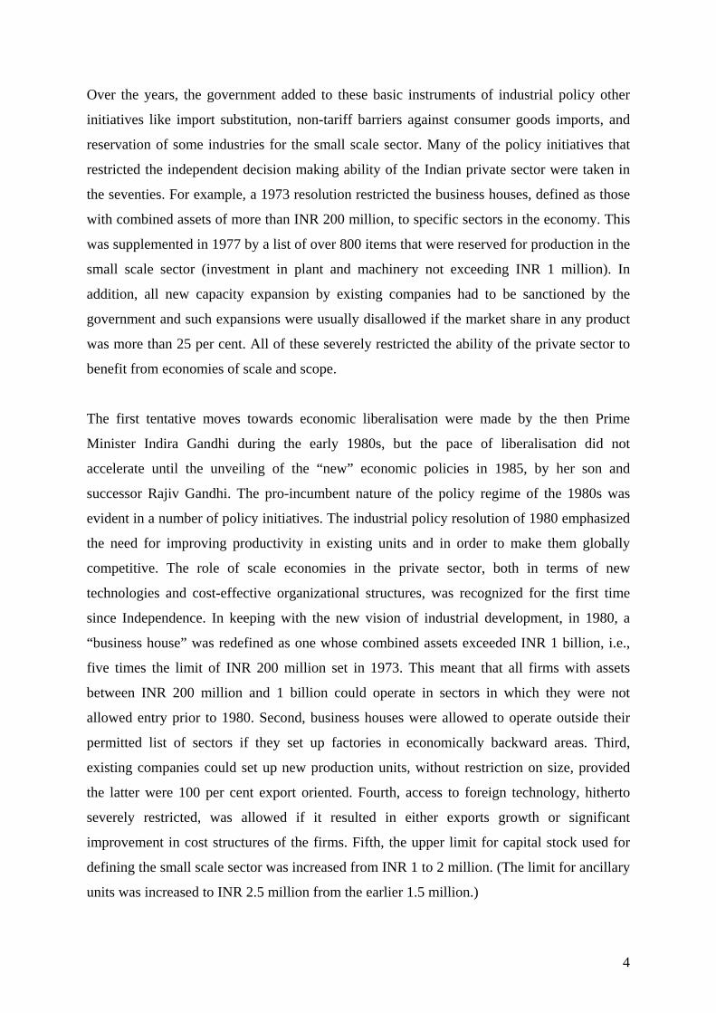
The descriptive statistics indicate that there was a growth in both gross value added and value

of the factor inputs, namely, capital and labour, between 1989-90 and 2000-01. The relative

magnitudes of the changes indicate that, for most industries, the growth rates in the labour

cost were very similar to the growth of the value added. However, the growth rate of capital

was much higher for all industries except paper, paper products and printing. This is

consistent with the view that there was significant capacity expansion in the Indian

manufacturing sector in the immediate aftermath of the 1991 reforms (Uchikawa, 2001,

2002). These growth rates of value added and the factor inputs for all the industries included

in our analysis are reported in Figure 1.

INSERT Figure 1 about here.

Given that the growth rate of capital exceeds the growth rate of labour cost, it is reasonable to

hypothesise that labour productivity in 2000-01 would be higher than that in 1989-90.

However, to the extent that capital embodies new technology, addition to the capital stock

might have increased productivity of capital as well. The descriptive statistics also indicate

that, as argued by Kalirajan and Bhide (2004), we can expect changes in factor inputs to

explain a significant proportion of the changes in gross value added between 1989-90 and

2000-01. In other words, changes in factor inputs and their productivity may explain much of

the growth in value added between the two years, as opposed to a change in technical

efficiency. We shall revisit this issue later in the paper.

4. Stochastic Frontier and Measurement of Technical Efficiency

The neo-classical production theory implicitly assumes that all production activities are on

the frontier of a feasible production set (subject to random errors). The frontier itself is

defined as of the maximum possible output that is technically attainable for the given inputs

(output-oriented measure), or as the observed output level that can be produced using lesser

inputs (input-oriented measure). The production efficiency literature, however, relaxes the

assumption, and considers the possibility that producers may operate below the frontier due

to technical inefficiency. Technical efficiency can be output-oriented if actual output

9

produced is less than the frontier output for a given amount of input (subject to random

errors). Alternatively, it can be input oriented if the amount of inputs actually used is more

than the minimum required to produce a given level of output. Graphically, the inefficient

production plans are located below the production frontier.

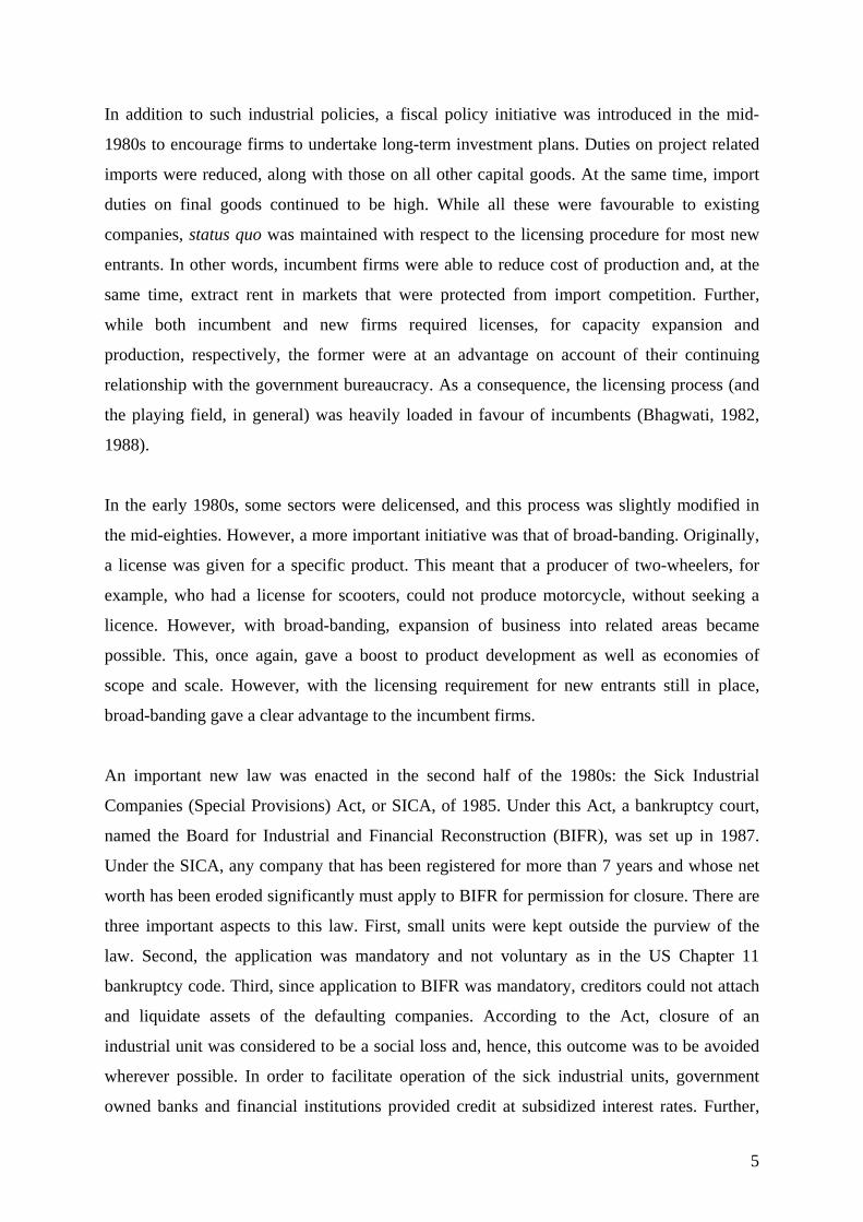
INSERT Figure 2 about here.

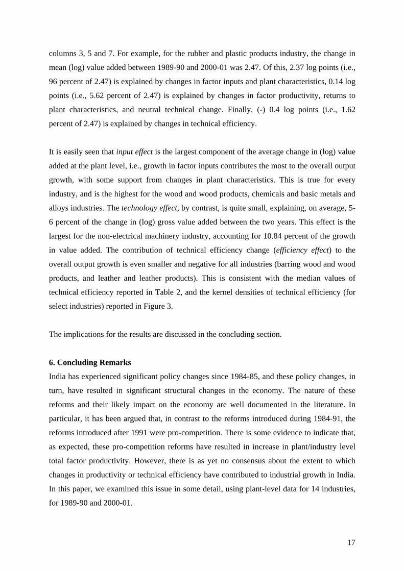
In Figure 2, f(x) is the production frontier, and point A is an inefficient production point.

There are two ways to see why it is inefficient. The first way is to see that at the current level

of input x more output can be produced, given the technology. The distance AB shows the

amount of output that is lost due to the technical inefficiency, and it forms the basis from

which the output-oriented (OO) technical inefficiency can be measured. The other way to see

why point A is inefficient is to recognize that the same level of output can be produced using

less inputs, which means that the production point can move to the frontier by reducing

inputs. The distance AC measures the amount by which the input can be reduced without

reducing output. Since this move is associated with reducing inputs, the horizontal distance

AC forms the basis to measure the input-oriented (IO) technical inefficiency.

Mathematically, a production plan with IO technical inefficiency is written as

( exp( )), 0y f x η η= − ≥ (1)

where η measures IO technical inefficiency (TI), and exp(-η ) measures IO technical

efficiency (TE). For small η , exp(-η ) can be approximated by 1 -η . Thus, we get the

following familiar relationship, TE = 1 - TI, which is clear from the above figure since

OB/OA=1-AB/OA.

A mathematical formulation of OO technical inefficiency is

( ) exp( ), 0y f x u u= − ≥ (2)

where u measures OO technical inefficiency. Again for small u we can approximate exp(-u)

by 1-u, which gives us the familiar result, TE = exp(-u) = 1 - u = 1 - TI.

Since inefficiency can be viewed either in the input or output direction, we get the following

relationship between the two measures, viz., ( ) exp( )f x u− = ( .exp( ))f x η− . If the production

function is homogeneous of degree k (which is nothing but returns to scale) then these two

10

inefficiency measures follow the relationship, .k uη = . That is, OO inefficiency is a constant

multiple (returns to scale) of IO inefficiency. In the special case when returns to scale is

unity, both inefficiency measures are the same. If returns to scale is neither constant nor

unity, the relationship is more complicated (although exact and is given by ( ) exp( )f x u− =

( .exp( ))f x η− ) and it depends on the input quantities.

For econometric estimation, a parametric function form on f(.) is assumed and a

multiplicative noise component is appended in the production relations in (1) and (2). This is

more realistic in the sense that there are uncertainties and possible omitted variables that can

affect output, given the technology and input quantities. In estimating efficiency the impact

of these uncertainties are to be accounted for. Since inefficiency is not observed, the

production function specified in either (1) or (2) cannot be estimated using OLS. At least the

use of OLS in a cross-sectional set-up will not give estimates of inefficiency for each

observation. For estimating inefficiency and production function parameters the maximum

likelihood (ML) method is used. The ML method is based on distributional assumptions on

the random and inefficiency terms. That is, for estimation point of view, especially in a cross-

sectional set-up one has to assume inefficiency to be a random variable. For the producer it

may be known but not to the analyst/econometrician. Once the model parameters are

estimated (in)efficiency for each observation can be obtained.

The standard distributional assumptions are: (i) the noise term (v) is independently normally

distributed with zero mean and constant variance, i.e., 2~ (0, )vv N σ (ii) the inefficiency term

is independently distributed as half-normal (zero mean, constant variance normal truncated at

zero from below – to make it non-negative), i.e., , (iii) the inefficiency and

noise components are assumed to be independent of each other and are also independent of

the inputs

2~ (0, ), 0uu N uσ ≥

9. Assuming that the production function is Cobb-Douglas (CD) the output-oriented

(OO) technical inefficiency model can be written as

9 Various other distributions for inefficiency such as exponential, gamma, truncated normal have been used in the literature. The estimates of inefficiency are in most cases quite robust to distributional assumptions. Models are developed to allow correlation between the noise and inefficiency components. Such correlations may not be very intuitive. Independence of inefficiency and inputs can be relaxed in a panel model as well as in models that introduce behavioral assumptions (such as cost minimization and profit maximization) explicitly. See Kumbhakar and Lovell (2000) for a survey of these models.

11

01

ln lnJ

j jj

y xβ β=

= + + −∑ v u (3)

Based on the above distributional assumptions the likelihood function of v uε = − can

be written as (see Kumbhakar and Lovell, 2000)

2L ε λ εφσ σ σ

⎡ ⎤ ⎡ ⎤= Φ −⎢ ⎥ ⎢ ⎥

⎣ ⎦ ⎣ ⎦ (4)

where 2 2 2v uσ σ σ= + /u v, λ σ σ= and ln ln ( )y f xε = − . Finally, 0

1ln ( ln )

J

j jj

y xβ β=

= − +∑

(.) and ( )φ Φ ⋅ are the probability density and distribution function, respectively, of a standard

normal variable. The logarithm of the above likelihood function (after adding it over all the

observations) can be maximized to obtain ML estimates of all the parameters in the model.

Once the parameters are estimated, one can obtain observation-specific technical inefficiency

from the conditional mean of u given ε , viz.,

*** *

* *

( / )E(u| ) = +

1 ( / )

φ µ σε µ σ

µ σ

−⎡ ⎤⎢−Φ −⎢ ⎥⎣ ⎦

⎥

2v

(5)

where 2 2 2 2 2* / and /u uµ εσ σ σ σ σ σ= − = . If the interest is to obtain observation-specific

estimates of technical efficiency, the following formula can be used

2**

*

1 ( / ) 1TE = [exp( | )] = exp1 ( / ) 2

E u σ µ σε µ σµ σ

∗ ∗∗

∗

⎡ ⎤−Φ − ⎧ ⎫− − +⎨ ⎬⎢ ⎥−Φ − ⎩ ⎭⎣ ⎦ (6)

The above formulation shows how to estimate the model and obtain observation-specific

estimates of technical (in)efficiency using the OO formulation. The IO formulation is more

complex (see Kumbhakar and Tsionas, 2006 for details). Instead of directly estimating the IO

model, one can estimate the OO model and obtain input-oriented inefficiency measure for

each observation from the relationship ( ) exp( )f x u− = ( .exp( ))f x η− which for the translog

production function can be expressed as 2

1 1( ) .5 J J

jkk ju RTS xη η

= == + ∑ ∑ β

j

(7)

where 1 1

( ) lnJ Jj jkj k

RTS x xβ β= =⎡= +⎣∑ ∑ ⎤

⎦ . One can solve for η from (7) once the

parameters estimates including u are known. This way one can avoid the complicated

econometric model of Kumbhakar and Tsionas (2006) at the expense of solving one quadratic

equation for each observation.

12

5. Econometric Models and Results

In the empirical model we use two inputs, viz., labour and capital, each measured in terms of

Indian rupees, i.e., we use labour cost instead of the total number of labourers. This measure

of labour, allows us to control for heterogeneity in labour quality across plants.10 Our model

specification also includes a vector of other attributes such as plant age and ownership types,

some of which may affect both output and efficiency.

Specifically, we take into consideration the possibility that technical efficiency and

productivity of labour and capital may vary across firms/plants of different ownership. It is

stylized in the literature that ownership has significant impact on firm-level productivity, and

that, on average, privately owned firms are more productive than state-owned firms (see, e.g.,

Hill and Snell, 1989; Ehrlich et al., 1994). It has also been argued that joint ventures between

the state and public entrepreneurs may not be as efficient as firms that are entirely privately

owned (Jin and Qian, 1998). In the Indian context, Majumdar (1998) has demonstrated that

this hierarchical order, namely, that private firms are more efficient than firms with mixed

ownership which, in turn, are more efficient than state-owned firms, holds true in India as

well. As evident from Table 1, our sample for each sector is overwhelmingly dominated by

privately owned plants, such that state-owned and joint sector plants each account for a very

small fraction of the sample. Hence, we include in the specification a solitary control for

ownership that takes the value unity when the plant is privately owned.

Finally, in the Indian context, there is reason to believe that firm performance might be

influenced by the location of the plant, given the significant diversity of infrastructure

quality, human capital, etc., across the Indian states (Bhaumik, Gangopadhyay and Krishnan,

2006). Hence, we use control for location using dummy variables for the states; Delhi is the

omitted category.

For each of the fourteen industries, we estimate the following augmented Cobb-Douglas

specification for simplicity11:

10 For a discussion about the potential biases associated with the use of labour hours as a measure for labour in the context of estimation of production functions, see Feldstein (1967). 11 Similar qualitative results were obtained from the translog form, especially the capital and labour elasticities at the mean. However, we found some implausible elasticities at many other points. Although this is not unusual for a translog function, we decided not to use it simply because these implausible results occurred at too many points.

13

(8) 0 1 2 3 4ln ln lnn

j jj i

y k l AGE PVT DS v uβ β β β β ρ=

= + + + + + + −∑

when y is output, l is labour, k is capital, AGE is plant age,12 PVT is the dummy variable that

controls for ownership, DSj is dummy for state/location j, and v and u have properties that

were discussed earlier in the paper.

INSERT Table 2 about here.

The parameter estimates are reported in Table 2. The results suggest the following:

Marginal productivity of capital in the formal manufacturing sector in India is much

lower than the marginal productivity of labour.13 This indicates that the plants or

production units are over-capitalised, which is not surprising in view of Indian labour

laws that generally make it difficult for a company to lay off labourers during periods

of low profitability (see Besley and Burgess, 2004).

There was an increase in the returns to both factor inputs between 1989-90 and 2000-

01. However, the percentage change in the returns to capital is much more significant

than the corresponding change in the returns to labour, even though, as indicated

earlier, the rate of growth of capital stock during the 1990s was much than the growth

in labour cost. This is perhaps a reflection of both a significant upgrade in the quality

of technology that is embodied in the capital, and an improvement in the skill of the

labour force that use the capital stock during the production process.

There was an increase in the returns to scale (RTS), such that the RTS in 2000-01

were much closer to 1 than those in 1989-90. In other words, in 2000-01, an average

manufacturing sector plant in the Indian manufacturing sector was operating much

closer to the minimum point of its long run average cost curve than in 1989-90. This

12 We experimented with several functional forms involving plant age, and it was evident that the logarithm of plant age best fit the data. 13 It is easily seen from Table 1 that the average values of plant-level capital and labour cost are roughly equal for all the industries. Hence, the difference in marginal productivity of these two factor inputs depends primarily on the difference between the estimated coefficients of (log) capital and (log) labour.

14

is consistent with the Rodrik and Subramanian (2004) argument that the policy

environment in India was much more pro-competition in the 1990s than in the 1980s.

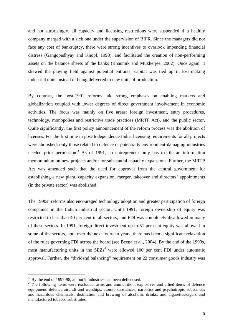
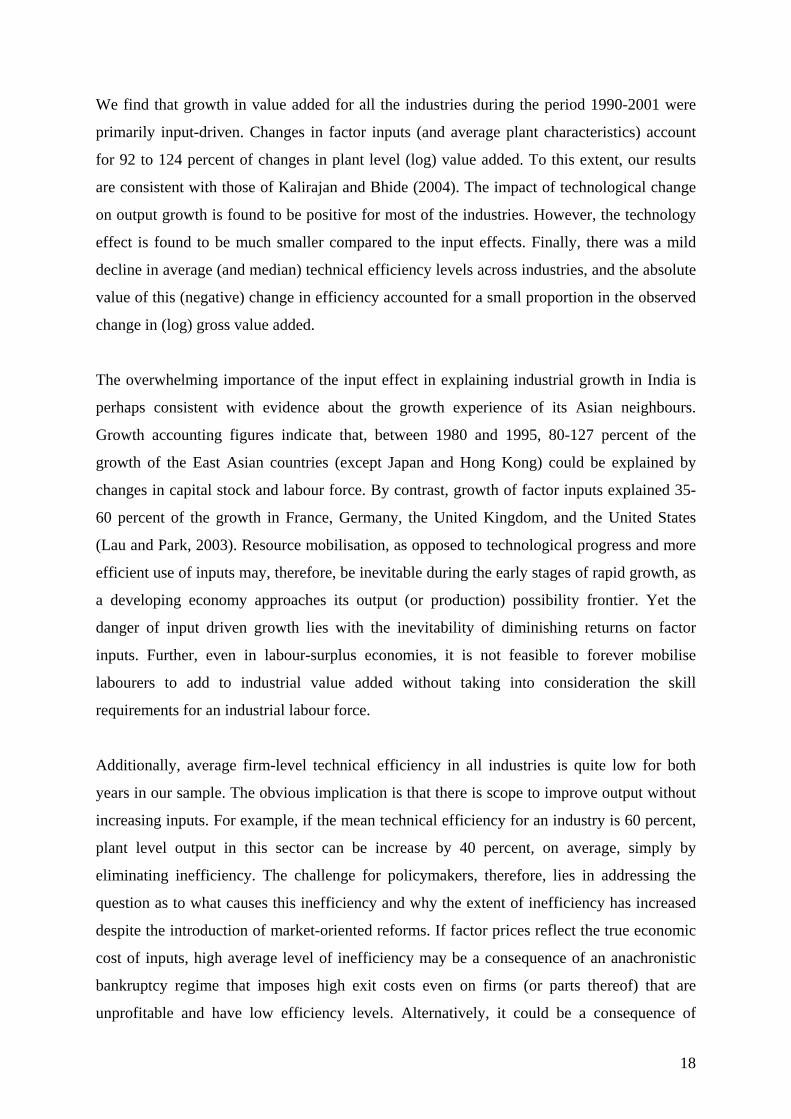
There was a noticeable decline in the median (and mean) level of technical efficiency

for each industry between 1989-90 and 2000-01. For each industry, z-statistics (t-

statistics), not reported in this paper, rejected the null hypothesis of equality of

median (mean) values of technical efficiency across the two years, in favour of the

alternative hypothesis that the median (mean) in 1989-90 is higher than that in 2000-

01. This is also evident from the distributions of plant-level technical efficiency for a

sample of industries that are reported in Figure 3.

INSERT Figure 3 about here.

Overall, the coefficient estimates and the estimates of technical efficiency indicate that

changes in returns to factor inputs can partially account for the changes in gross value added

between the two years, but that changes in technical efficiency would not be able to explain

the growth in gross value added to a significant extent. In order to better understand the

relative impact of changes in factor inputs, returns to these inputs and technical efficiency on

growth of average gross value added of the 14 industries, we undertake a decomposition

analysis.

The methodology used for the decomposition is analogous to that of Oaxaca (1973). Suppose

that the estimated production functions for 1989-90 (year 1) and 2000-01 (year 2) are as

follows:

(9) 1

'1 1 1 1

ˆˆy X vα β= + + − 1u

2u (10) 2

'2 2 2 2

ˆˆy X vα β= + + −

when y is the (log) value added, X is a vector of variables including (log) labour cost and

(log) capital, v is the iid error term, and u is the inefficiency term with a half-normal

distribution. As a matter of fact v-u in (9) and (10) are the ML residuals. It is easy to show

that the difference between the average (log) value added between the two time periods is

given by

2 2 1

' ' '2 1 2 1 2 1 1 2 1 2 1

ˆ ˆ ˆˆ ˆ( ) ( ) ( ) ( ) (y y X X X v v u uα α β β β− = − + − + − + − − − ) (11)

15

It is, of course, obvious that the change in (log) value added, factor inputs etc. can be

estimated for each individual plant in the sample. However, for an individual plant, the iid

error term v need not equal zero; the mean of the distribution of the iid term across plants

equals zero, by assumption. Hence, it is stylised to undertake this decomposition exercise

using mean values for y and X.

Since the iid error term v has zero mean, the mean values of v1 and v2 will be zero (or close to

zero) and so is the 2 1(v v− ) term, which will be either zero or small enough to ignore.

Equation (11) can then be reduced to

2 2 1

' ' '2 1 2 1 2 1 1 2 1

ˆ ˆ ˆˆ ˆ( ) [( ) ( ) ] (y y X X X u uβ α α β β− = − + − + − − − )

(11a)

The first term on the right hand side of equation (11a) is the contribution of change in inputs

to growth of value added between two time periods. The second term is the contribution of

technology differences between the two time periods on output growth. It captures the impact

of changes in both factor productivity and returns to plant characteristics, as well as the

impact of neutral technical change on the value added.14 Finally, the last term captures the

contribution of the difference in technical efficiency to output growth. We label them input

effect, technology effect and efficiency effect, respectively.

INSERT Table 3 about here.

The decomposition results for each industry are reported in Table 3. In column 1 we report

the difference in the mean (log) value added between the two time periods for each industry.

It varies from 1.79 to 2.89 (log points) across industries. The contributions of input effect,

technology effect and efficiency effect to the growth in value added are reported in columns

2, 4 and 6, respectively, while the corresponding percentage contributions are reported in

)

14 One can further decompose technology effects into two components, namely, the growth in value added that can be attributed to changes in input productivity and returns to plant characteristics (j),

2 1ˆ ˆ( j j jxβ β− , and to the difference in the intercept term ( 2ˆ ˆ1α α− ). It is tempting to argue that the

constant or intercept term in a log production function represents x-efficiency (see Jovanovic and Gilbert, 1993). When viewed from this perspective, the difference in the estimated constant terms of the regression models captures the effect of change in the average managerial quality and x-efficiency between the two time periods on output growth. However, it is also likely to capture differences in neutral technical change. Given the ten-year gap in the data, which is necessary to facilitate a discussion about the impact of reforms in India, it is difficult for us to intuitively distinguish between technical change and x-efficiency. Hence, we are not interpreting the differences in the intercept terms as the effect of changes in x-efficiency on output growth.

16

columns 3, 5 and 7. For example, for the rubber and plastic products industry, the change in

mean (log) value added between 1989-90 and 2000-01 was 2.47. Of this, 2.37 log points (i.e.,

96 percent of 2.47) is explained by changes in factor inputs and plant characteristics, 0.14 log

points (i.e., 5.62 percent of 2.47) is explained by changes in factor productivity, returns to

plant characteristics, and neutral technical change. Finally, (-) 0.4 log points (i.e., 1.62

percent of 2.47) is explained by changes in technical efficiency.

It is easily seen that input effect is the largest component of the average change in (log) value

added at the plant level, i.e., growth in factor inputs contributes the most to the overall output

growth, with some support from changes in plant characteristics. This is true for every

industry, and is the highest for the wood and wood products, chemicals and basic metals and

alloys industries. The technology effect, by contrast, is quite small, explaining, on average, 5-

6 percent of the change in (log) gross value added between the two years. This effect is the

largest for the non-electrical machinery industry, accounting for 10.84 percent of the growth

in value added. The contribution of technical efficiency change (efficiency effect) to the

overall output growth is even smaller and negative for all industries (barring wood and wood

products, and leather and leather products). This is consistent with the median values of

technical efficiency reported in Table 2, and the kernel densities of technical efficiency (for

select industries) reported in Figure 3.

The implications for the results are discussed in the concluding section.

6. Concluding Remarks

India has experienced significant policy changes since 1984-85, and these policy changes, in

turn, have resulted in significant structural changes in the economy. The nature of these

reforms and their likely impact on the economy are well documented in the literature. In

particular, it has been argued that, in contrast to the reforms introduced during 1984-91, the

reforms introduced after 1991 were pro-competition. There is some evidence to indicate that,

as expected, these pro-competition reforms have resulted in increase in plant/industry level

total factor productivity. However, there is as yet no consensus about the extent to which

changes in productivity or technical efficiency have contributed to industrial growth in India.

In this paper, we examined this issue in some detail, using plant-level data for 14 industries,

for 1989-90 and 2000-01.

17

We find that growth in value added for all the industries during the period 1990-2001 were

primarily input-driven. Changes in factor inputs (and average plant characteristics) account

for 92 to 124 percent of changes in plant level (log) value added. To this extent, our results

are consistent with those of Kalirajan and Bhide (2004). The impact of technological change

on output growth is found to be positive for most of the industries. However, the technology

effect is found to be much smaller compared to the input effects. Finally, there was a mild

decline in average (and median) technical efficiency levels across industries, and the absolute

value of this (negative) change in efficiency accounted for a small proportion in the observed

change in (log) gross value added.

The overwhelming importance of the input effect in explaining industrial growth in India is

perhaps consistent with evidence about the growth experience of its Asian neighbours.

Growth accounting figures indicate that, between 1980 and 1995, 80-127 percent of the

growth of the East Asian countries (except Japan and Hong Kong) could be explained by

changes in capital stock and labour force. By contrast, growth of factor inputs explained 35-

60 percent of the growth in France, Germany, the United Kingdom, and the United States

(Lau and Park, 2003). Resource mobilisation, as opposed to technological progress and more

efficient use of inputs may, therefore, be inevitable during the early stages of rapid growth, as

a developing economy approaches its output (or production) possibility frontier. Yet the

danger of input driven growth lies with the inevitability of diminishing returns on factor

inputs. Further, even in labour-surplus economies, it is not feasible to forever mobilise

labourers to add to industrial value added without taking into consideration the skill

requirements for an industrial labour force.

Additionally, average firm-level technical efficiency in all industries is quite low for both

years in our sample. The obvious implication is that there is scope to improve output without

increasing inputs. For example, if the mean technical efficiency for an industry is 60 percent,

plant level output in this sector can be increase by 40 percent, on average, simply by

eliminating inefficiency. The challenge for policymakers, therefore, lies in addressing the

question as to what causes this inefficiency and why the extent of inefficiency has increased

despite the introduction of market-oriented reforms. If factor prices reflect the true economic

cost of inputs, high average level of inefficiency may be a consequence of an anachronistic

bankruptcy regime that imposes high exit costs even on firms (or parts thereof) that are

unprofitable and have low efficiency levels. Alternatively, it could be a consequence of

18

ownership structures that do encourage meritocratic choice of managers and, at the same

time, protect even inefficient firms from all forms of market discipline. We have already

discussed the problems with the Indian bankruptcy regime earlier in this paper. There is also

evidence to suggest that management succession in Indian firms, a large proportion of which

are group affiliated and family-owned (Piramal, 1996), is based on blood connection as

opposed to merit (Sharma and Rao, 2000), and that incidence of persistent bad-performance

is fairly common among group-affiliated Indian firms (Chacar and Vissa, 2005). Aside from

the obvious need to enact laws that makes it easy for inefficient firms to declare bankruptcy,

therefore, the way forward perhaps lies in developing institutions that facilitate corporate

takeovers which, in turn, breed market discipline and, hence, efficiency.

19

References Aghion, Philippe and Robin Burgess (2003). Liberalization and industrial performance: Evidence from India and the UK. Mimeo, London School of Economics, http://www.ycsg.yale.edu/activities/files/Aghion-Burgess%20Paper.pdf. Beena, P.L. et al. (2004). Foreign Direct Investment in India. In Saul Estrin and Klaus E. Meyer (Eds.) Investment Strategies in Emerging Markets, Edward Elgar, Cheltenham, 2004. Besley, Timothy and Robin Burgess (2004). Can labor regulation hinder economic performance? Evidence from India. Quarterly Journal of Economics, 119(1), 91-134. Bhagwati, Jagdish N. (1982). Directly unproductive, profit-seeking (DUP) activities, Journal of Political Economy, 90, 988-1002. Bhagwati, Jagdish N. (1988). “Export-promoting trade strategies: Issues and evidence, World Bank Research Observer, 3(1), 27-57. Bhaumik, Sumon K and Paramita Mukherjee (2002). The Indian banking sector: A commentary. In: Parthasarathi Banerjee and Frank-Jurgen Richter (Eds.) Economic Institutions in India: Sustainability under Liberalization and Globalization, Palgrave Macmillan, London. Bhaumik, Sumon K., Shubhashis Gangopadhyay and Shagun Krishnan (2006). Reforms, entry and productivity: Some evidence from the Indian manufacturing sector. Discussion paper no. 2086, IZA – Institute for Study of Labour, Bonn. Chacar, Aya and Balagopal Vissa (2005). Are emerging economies less efficient? Performance persistence and business group affiliation. Strategic Management Journal, 26(10): 933-946. Chand, Satish and Kunal Sen (2002). Trade liberalization and productivity growth: Evidence from Indian manufacturing. Review of Development Economics, 6(1), 120-132. Driffield, Nigel L. and Uma S. Kambhampati (2003). Trade liberalization and the efficiency of firms in Indian manufacturing. Review of Development Economics, 7(3): 419-430. Ehrlich, Issac et al. (1994). Productivity Growth and Firm Ownership: An Analytical and Empirical Investigation. Journal of Political Economy, 102(5), 1006-1038. Feldstein, Martin S. (1967). Specification of the labour input in the aggregate production function. Review of Economic Studies, 34(4), 375-386. Gangopadhyay, Shubhashis and John D. Knopf (1998). Dividends and conflicts between equityholders and debtholders with weak monitoring: The case of India. In: John Doukas, Victor Murinde and Clas Wihlborg (Eds.) Financial Sector Reform and Privatization in Transition Economies, North-Holland, Amsterdam.

20

Hasan, Rana, Devashish Mitra and K.V. Ramaswamy (2003). Trade reforms, labor regulations and labor demand elasticities: Empirical evidence from India. Working paper no. 9879, National Bureau of Economic Research, Cambridge, Massachusetts. Hill, Charles W.L. and Scott A. Snell (1989). Effects of Ownership Structure and Control on Corporate Productivity. Academy of Management Journal, 32(1), 25-46. Jin, Hehui and Yingyi Qian (1998). Public versus Private Ownership of Firms: Evidence from Rural China. Quarterly Journal of Economics, 113(3), 773-808. Jovanovic, Boyan and Richard J. Gilbert (1993). The diversification of production. Brookings Papers on Economic Activity – Microeconomics, No. 1, 197-247. Kaliappa, Kalirajan and Shashanka Bhide (2004). The post-reform performance of the manufacturing sector in India. Asian Economic Papers, 3(2), 126-157. Krishna, Pravin and Devashish Mitra (1998). Trade liberalisation, market discipline and productivity growth: New evidence from India. Journal of Development Economics, 56, 447-462. Kumar, Surender (2006). A decomposition of total productivity growth: A regional analysis of Indian industrial manufacturing growth. International Journal of Productivity and Performance Management, 55(3-4), 311-311. Kumbhakar, Subal and C. A. Knox Lovell (2000), Stochastic Frontier Analysis, Cambridge University Press, New York. Kumbhakar, Subal and Tsionas, E.G. (2006). Estimation of Stochastic Frontier Production Functions with Input-Oriented Technical Efficiency, Journal of Econometrics, 133, 71-96. Lall, Somik V. and Sanjoy Chakravorty (2005). Industrial location and spatial inequality: Theory and evidence from India. Review of Development Economics, 9(1), 47-68. Lau, Lawrence J. and Jungsoo Park (2003). The sources of East Asian economic growth Revisited. Mimeo, Stanford University, http://www.stanford.edu/~ljlau/RecentWork/RecentWork/030921.pdf. Li, Wei (1997). The impact of economic reform on the performance of Chinese state enterprises, 1980-89. Journal of Political Economy, 105(5), 1080-1106. Majumdar, Sumit K (1998). Assessing comparative efficiency of the state owned, mixed and private sectors in Indian industry. Public Choice, 96(1-2), 1-24. Oaxaca, Ronald (1973). Male-female wage differentials in urban labor markets. International Economic Review, 14(3), 693-709. Piramal, Gita (1996). Business maharajas. New Delhi, India: Penguin Books. Rodrik, Dani and Arvind Subramanian (2004). From “Hindu growth” to productivity surge: The mystery of the Indian growth transition. IMF Staff Papers, 52(2), 193-228.

21

Sharma, P. and A.S. Rao (2000). Successor attributes in Indian and Canadian family firms: A comparative study. Family Business Review, 13, 313-330. Sivadasan, Jagdeesh (2003). Barriers to entry and productivity: Micro-evidence from Indian manufacturing sector reforms. Mimeo, University of Chicago, http://bpp.wharton.upenn.edu/Documents/Sivadasan_AEW_paper_1_16_04.pdf. Topalova, Petya (2004). Trade liberalization and firm productivity: The case of India. Working paper no. WP/04/28, International Monetary Fund, Washington, D.C. Uchikawa, Suchi (2001). Investment boom and underutilisation of capacity in the 1990s, Economic and Political Weekly, 34 (August 25), 3247-3254. Uchikawa, Suchi (2002). Investment boom and the capital goods industry. In Suchi Uchikawa (Ed.), Economic Reforms and Industrial Structure in India, New Delhi: Manohar Publishers.

22

Table 1: Descriptive statistics

Industry

Year

Log gross

value added

Log capital

Log labour cost

Log plant age

Percentage of plants in private

sector

1989-90 13.34 13.15 12.34 2.42 95.43 Agricultural products 2000-01 16.07 16.59 14.96 2.67 81.72

1989-90 13.47 13.46 12.70 2.26 92.78 Textiles (without

apparel) 2000-01 16.15 17.22 15.33 2.64 87.51

1989-90 13.43 12.84 12.51 2.17 98.67 Textile products 2000-01 15.73 15.45 14.87 2.01 99.03

1989-90 12.50 12.01 11.70 2.38 96.24 Wood & wood products 2000-01 15.07 15.93 14.62 2.38 100.00

1989-90 13.31 13.49 12.38 2.44 96.90 Paper, paper

products & printing 2000-01 14.92 15.17 14.09 2.30 96.43

1989-90 13.83 13.58 12.93 1.99 97.44 Leather & leather products 2000-01 15.71 16.13 14.51 2.61 96.89

1989-90 13.63 13.22 12.63 2.26 97.21 Chemicals &

chemical products 2000-01 16.02 16.56 15.02 2.61 93.73

1989-90 13.28 13.61 12.25 2.06 97.56 Rubber & rubber products 2000-01 15.66 16.33 14.31 2.33 94.76

1989-90 12.89 12.65 12.21 2.24 97.41 Non-metallic

products 2000-01 15.58 16.40 14.63 2.52 94.93

1989-90 13.61 13.57 12.64 2.69 98.39 Basic metals & alloys 2000-01 15.86 16.71 14.78 2.49 95.95

1989-90 13.00 12.84 12.12 2.38 97.90 Metals & metal

products 2000-01 15.33 15.59 14.49 2.38 94.94

1989-90 13.34 13.15 12.46 2.49 97.86 Non-electrical machinery 2000-01 15.57 15.63 14.75 2.73 96.38

1989-90 13.51 13.27 12.63 2.13 96.62 Electrical

machinery & equipment 2000-01 15.69 15.82 14.80 2.64 94.73

1989-90 13.49 13.34 12.59 2.35 98.47 Transport

equipment 2000-01 16.32 16.79 15.36 2.51 96.11

23

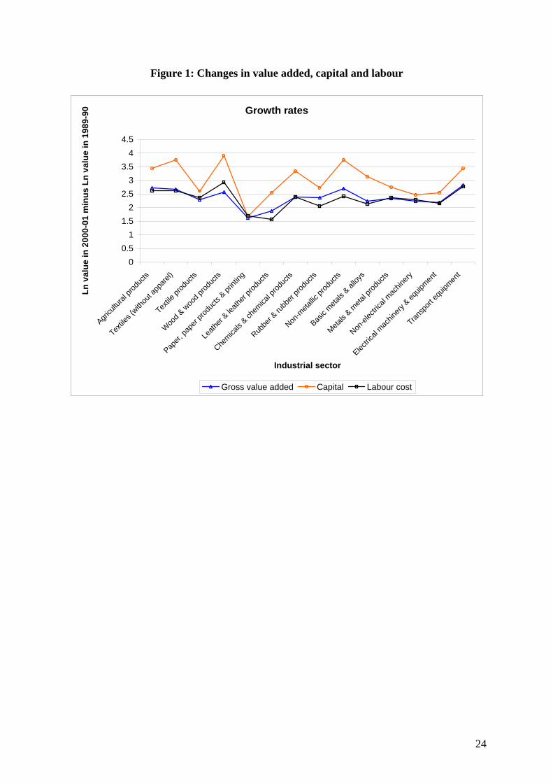
Figure 1: Changes in value added, capital and labour

Growth rates

00.5

11.5

22.5

33.5

44.5

Agricu

ltural

prod

ucts

Textile

s (with

out a

ppare

l)

Textile

prod

ucts

Woo

d & w

ood p

roduc

ts

Paper,

pape

r prod

ucts

& print

ing

Leath

er & le

ather

produ

cts

Chemica

ls & ch

emica

l prod

ucts

Rubbe

r & ru

bber

produ

cts

Non-m

etallic

prod

ucts

Basic

metals

& alloy

s

Metals

& meta

l prod

ucts

Non-el

ectric

al mac

hinery

Electric

al mac

hinery

& eq

uipmen

t

Transp

ort eq

uipmen

t

Industrial sector

Ln v

alue

in 2

000-

01 m

inus

Ln

valu

e in

198

9-90

Gross value added Capital Labour cost

24

Figure 2: Technical efficiency

y

OO A

O

y = f(x)

O M N x

C

I

B

25

Table 2: Coefficient estimates of production function

Industry

Year

Constant [β0]

Capital [β1]

Labour [β2]

Plant age [β3]

Private [β4]

Wald χ2

(Prob > χ2)

Nobs Returns to

Scale Technical Efficiency

1989-90 2.13 *** (0.15)

0.16 *** (0.01)

0.76 *** (0.01)

0.04 *** (0.01)

0.42 *** (0.05)

10834.44 (0.00)

4635 0.92 0.55 Agricultural

products 2000-01 1.83 *** (0.27)

0.23 *** (0.02)

0.77 *** (0.02)

- 0.14 *** (0.03)

0.51 *** (0.07)

4675.89 (0.00)

1547 1.00 0.52

1989-90 2.34 *** (0.17)

0.21 *** (0.01)

0.68 *** (0.01)

- 0.03 ** (0.01)

0.51 *** (0.05)

8109.54 (0.00)

2618 0.89 0.59 Textiles (without

apparel) 2000-01 1.87 *** (0.25)

0.27 *** (0.01)

0.68 *** (0.02)

- 0.22 *** (0.03)

0.75 *** (0.07)

6188.50 (0.00)

1377 0.95 0.54

1989-90 2.09 *** (0.34)

0.17 *** (0.02)

0.75 *** (0.02)

0.03 (0.02)

0.17 (0.17)

2320.99 (0.00)

979 0.92 0.62

Textile products 2000-01 1.04

(0.79) 0.11 *** (0.03)

0.87 *** (0.04)

- 0.01 (0.05)

0.13 (0.43)

815.98 (0.00)

307 0.98 0.58

1989-90 1.71 *** (0.29)

0.17 *** (0.02)

0.76 *** (0.03)

- 0.002 (0.03)

0.44 *** (0.11)

2827.20 (0.00)

797 0.93 0.60 Wood & wood

products 2000-01 1.42 * (0.73)

0.27 *** (0.06)

0.71 *** (0.07)

- 0.11 (0.07)

-- 850.21 (0.00)

171 0.98 0.65

1989-90 2.14 *** (0.20)

0.20 *** (0.01)

0.74 *** (0.02)

- 0.10 *** (0.02)

0.18 ** (0.09)

5285.22 (0.00)

1503 0.94 0.61 Paper, paper

products & printing 2000-01 0.83 (0.85)

0.14 *** (0.03)

0.89 *** (0.05)

- 0.16 *** (0.06)

0.41 (0.31)

920.07 (0.00)

280 1.03 0.52

1989-90 2.43 *** (0.65)

0.23 *** (0.03)

0.67 *** (0.05)

- 0.07 * (0.04)

0.12 (0.25)

674.32 (0.00)

351 0.90 0.53 Leather & leather

products 2000-01 0.87 * (0.48)

0.13 *** (0.01)

0.95 *** (0.03)

- 0.22 *** (0.04)

0.13 (0.26)

2486.92 (0.00)

482 1.08 0.61

26

1989-90 3.25 *** (0.25)

0.13 *** (0.01)

0.73 *** (0.02)

- 0.03 (0.02)

0.13 (0.10)

3378.49 (0.00)

1857 0.86 0.56 Chemicals &

chemical products 2000-01 0.59 * (0.33)

0.25 *** (0.02)

0.80 *** (0.02)

- 0.12 *** (0.04)

0.29 ** (0.12)

5521.74 (0.00)

1192 1.05 0.51

1989-90 2.04 *** (0.27)

0.24 *** (0.01)

0.72 *** (0.02)

- 0.03 (0.02)

0.02 (0.14)

3922.75 (0.00)

1586 0.96 0.55 Rubber & plastic

products 2000-01 0.85 * (0.50)

0.36 *** (0.03)

0.71 *** (0.04)

- 0.15 *** (0.06)

0.05 (0.18)

4541.50 (0.00)

534 1.07 0.53

1989-90 2.19 *** (0.17)

0.13 *** (0.01)

0.77 *** (0.01)

- 0.01 (0.01)

0.18 ** (0.07)

7322.74 (0.00)

2221 0.90 0.60 Non-metallic

products 2000-01 0.99 *** (0.35)

0.33 *** (0.02)

0.70 *** (0.02)

- 0.15 *** (0.03)

0.18 (0.19)

5024.96 (0.00)

586 1.03 0.56

1989-90 3.24 *** (0.24)

0.18 *** (0.01)

0.69 *** (0.02)

- 0.04 ** (0.02)

- 0.11 (0.12)

4825.73 (0.00)

1854 0.87 0.56 Basic metals &

alloys 2000-01 0.79 * (0.42)

0.36 *** (0.03)

0.66 *** (0.04)

- 0.16 *** (0.05)

0.60 *** (0.16)

3625.48 (0.00)

615 1.02 0.51

1989-90 1.99 *** (0.20)

0.17 *** (0.01)

0.77 *** (0.02)

- 0.03 * (0.02)

0.09 (0.07)

5182.09 (0.00)

1993 0.94 0.64 Metals & metal

products 2000-01 1.17 ** (0.52)

0.16 *** (0.03)

0.88 *** (0.04)

- 0.21 *** (0.05)

0.13 (0.23)

1716.46 (0.00)

434 1.04 0.54

1989-90 2.15 *** (0.17)

0.19 *** (0.01)

0.73 *** (0.01)

- 0.05 *** (0.01)

0.07 (0.08)

7947.23 (0.00)

2289 0.92 0.66 Non-electrical

machinery 2000-01 1.84 *** (0.36)

0.16 *** (0.02)

0.84 *** (0.03)

- 0.19 *** (0.03)

0.18 (0.16)

4827.25 (0.00)

884 1.00 0.56

Electrical 1989-90 2.19 *** (0.26)

0.19 *** (0.02)

0.73 *** (0.02)

0.001 (0.02)

0.30 *** (0.10)

3144.49 (0.00)

1617 0.92 0.53

27

machinery & equipment 2000-01 1.47 ***

(0.42) 0.25 *** (0.03)

0.77 *** (0.04)

- 0.15 *** (0.05)

- 0.02 (0.18)

3197.16 (0.00)

493 1.02 0.51

1989-90 2.24 *** (0.25)

0.16 *** (0.01)

0.74 *** (0.02)

- 0.07 *** (0.02)

0.35 *** (0.10)

4293.70 (0.00)

1176 0.90 0.68 Transport equipment 2000-01 0.82 **

(0.35) 0.24 *** (0.03)

0.78 *** (0.03)

- 0.16 *** (0.03)

0.32 * (0.17)

4901.29 (0.00)

591 1.02 0.60

Notes: The values within parentheses reported after the coefficient estimates (β) are robust standard errors. ***, ** and * indicate significance at 1%, 5% and 10% levels, respectively.

In 2000-01, 100% of the plants in the sample for the wood and wood products were privately owned, and hence the regression model for that industry did not have a control for ownership. The return to scale for each industry is the sum of the coefficients for log capital and log labour cost. The technical efficiency measure reported for each industry is the median technical efficiency for that industry.

28

Figure 3: Technical efficiency distributions in select industries

01

23

4

0 .2 .4 .6 .8 1x

kdensity te_198990_textiles kdensity te_200001_textiles

01

23

45

0 .2 .4 .6 .8 1x

kdensity te_198990_textileprod kdensity te_200001_textileprod

Textiles (without apparel) Textile products

01

23

4

0 .2 .4 .6 .8 1x

kdensity te_198990_leather kdensity te_200001_leather

01

23

0 .2 .4 .6 .8 1x

kdensity te_198990_chemical kdensity te_200001_chemical

Leather & leather products Chemicals

0.5

11.

52

2.5

0 .2 .4 .6 .8 1x

kdensity te_198990_basicmetal kdensity te_200001_basicmetal

01

23

45

0 .2 .4 .6 .8 1x

kdensity te_198990_machinery kdensity te_200001_machinery

Basic metals & alloys Non-electrical machinery

29

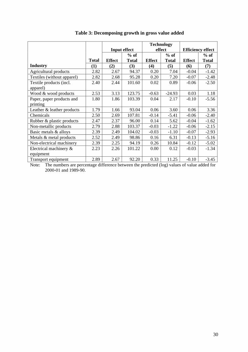
Table 3: Decomposing growth in gross value added

Input effect

Technology effect

Efficiency effect

Total

Effect % of Total

Effect

% of Total

Effect

% of Total

Industry (1) (2) (3) (4) (5) (6) (7) Agricultural products 2.82 2.67 94.37 0.20 7.04 -0.04 -1.42Textiles (without apparel) 2.82 2.68 95.28 0.20 7.20 -0.07 -2.48Textile products (incl. apparel)

2.40 2.44 101.60 0.02 0.89 -0.06 -2.50

Wood & wood products 2.53 3.13 123.75 -0.63 -24.93 0.03 1.18Paper, paper products and printing

1.80 1.86 103.39 0.04 2.17 -0.10 -5.56

Leather & leather products 1.79 1.66 93.04 0.06 3.60 0.06 3.36Chemicals 2.50 2.69 107.81 -0.14 -5.41 -0.06 -2.40Rubber & plastic products 2.47 2.37 96.00 0.14 5.62 -0.04 -1.62Non-metallic products 2.79 2.88 103.37 -0.03 -1.22 -0.06 -2.15Basic metals & alloys 2.39 2.49 104.02 -0.03 -1.10 -0.07 -2.93Metals & metal products 2.52 2.49 98.86 0.16 6.31 -0.13 -5.16Non-electrical machinery 2.39 2.25 94.19 0.26 10.84 -0.12 -5.02Electrical machinery & equipment

2.23 2.26 101.22 0.00 0.12 -0.03 -1.34

Transport equipment 2.89 2.67 92.20 0.33 11.25 -0.10 -3.45Note: The numbers are percentage difference between the predicted (log) values of value added for

2000-01 and 1989-90.

30