HAL Id: hal-02370399https://hal.archives-ouvertes.fr/hal-02370399

Submitted on 26 Nov 2020

HAL is a multi-disciplinary open accessarchive for the deposit and dissemination of sci-entific research documents, whether they are pub-lished or not. The documents may come fromteaching and research institutions in France orabroad, or from public or private research centers.

L’archive ouverte pluridisciplinaire HAL, estdestinée au dépôt et à la diffusion de documentsscientifiques de niveau recherche, publiés ou non,émanant des établissements d’enseignement et derecherche français ou étrangers, des laboratoirespublics ou privés.

Impact of Spray Droplet Distribution on thePerformances of a Kerosene Lean/Premixed Injector

Patricia Domingo-Alvarez, Pierre Benard, Ghislain Lartigue, VincentMoureau, Frederic Grisch

To cite this version:Patricia Domingo-Alvarez, Pierre Benard, Ghislain Lartigue, Vincent Moureau, Frederic Grisch. Im-pact of Spray Droplet Distribution on the Performances of a Kerosene Lean/Premixed Injector. Flow,Turbulence and Combustion, Springer Verlag (Germany), 2019, �10.1007/s10494-019-00073-5�. �hal-02370399�

Impact of spray droplet distribution on the performances of akerosene lean/premixed injector

PATRICIA DOMINGO-ALVAREZ1,∗, PIERRE BENARD1, GHISLAIN LARTIGUE1,VINCENT MOUREAU1, FREDERIC GRISCH1

1 CORIA, CNRS UMR6614, INSA and University of Rouen, Avenue de l’Universite,

76801 Saint-Etienne-du-Rouvray, France∗ Corresponding author: domingop@coria.fr

November 10, 2020

Abstract

Large-Eddy Simulation (LES) of a novel lean-premixed (LP) injection system for aeronautical burners is performed at elevated pressure/ temperature operating conditions. This LP injector was designed to operate at high-pressure and high-temperature and it was exper-imentally investigated at DLR Cologne and at CORIA laboratory in Rouen. At DLR Cologne, the purpose was to measure dropletssizes and velocities thanks to the Phase Doppler Anemometry (PDA) technique. At CORIA, combustion under realistic pressure con-ditions was investigated on the HERON test rig with advanced and combined optical diagnostics, such as OH and Kerosene PlanarLaser-Induced Fluorescence (PLIF). It was observed that the flame topology strongly depends on the pressure. This configuration istherefore an interesting validation database for LES. In this LP injector, liquid kerosene is injected far upstream of the injector in orderto provide a gaseous fuel distribution as homogeneous as possible. In the LES, the full geometry of the injector is taken into account.One reference operating point at 8.33 bar and 669.3K is simulated. A Lagrangian point-particle approach is chosen for the spraymodeling with a prescribed Rosin-Rammler diameter distribution at injection. The two-phase combustion model relies on a tabulatedchemistry approach. The flame/turbulence interactions are included via a presumed-PDF closure (PCM-FPI model). The impact ofspray characteristics on the flame is analyzed through a dedicated parametric study. Four sets of parameters each with a differentSauter Mean Diameter are used to describe the spray droplet size distribution. An analysis of the characteristic evaporation time andits influence on the flame has been carried out. Numerical results are then compared with experimental data in order to bring detailedinsights into the flame topology. This parametric study shows that the quality of the atomization strongly influences the flame topologyand the fuel distribution inside the combustion chamber.

Keywords: Large-Eddy Simulation Aeronautical burner LP injection system High-pressure Spray combustion

1 IntroductionThe ACARE 2020 objectives in the aviation transportation [1] plan a reduction of CO2 by 50%, a 50% reduction of theSpecific Fuel Consumption (SFC) and 80% reduction of the emission of NOx per passenger kilometer as well as 50%reduction of the noise compared to the levels in 2000. In order to reduce CO2 emissions and the SFC, aeronautical enginemanufacturers design new technologies allowing to increase the Overall Pressure Ratio (OPR). However, this rise in theOPR leads to a higher temperature in the combustion chamber, which in turn leads to the increase of NOx emissions. Tocounteract this issue, new innovative engine technologies using state-of-the-art injection technology such as lean premixed(LP) or variants are needed. In LP combustion, a homogeneous mixing is the key to lower the flame temperature, andthe subsequent thermal NOx, but it can affect the flame stability and other pollutant emissions [2, 3]. Most of theseperformances are directly related to the spray characteristics of the atomizer, thus the technology of fuel supply of theatomizer is very important [4]. The design of such injectors remains difficult and requires predictive models for theiroptimization. Different types of atomizers have been used in the industry for the injection of liquid fuel, yet all of themare based on the high relative velocity between the liquid and the surrounding gas. Many different types of atomizers havebeen experimentally studied during the past years, however the spray formation processes, the droplet dynamics and thefinal droplet size distributions are still not completely understood [6, 5].

Large-Eddy Simulation (LES) is an adequate framework for the modeling of the many complex physical phenomenainvolved in LP systems as it gives access to unsteady flow features at an affordable CPU cost [7]. It also provides small-scale dynamics that can be compared to high-frequency laser diagnostics. Spray combustion LES is able to reproducedroplet transport and evaporation with point-particle approaches [8, 9]. Some recent studies have been focused on the

1

process of breakup and atomization [10, 11, 12], however it involves complex physical processes and gas-liquid interac-tions and it needs a large number of cells or the use of adaptive meshes which entails a high computational cost. In mostsimulations of realistic injectors, atomization is not taken into account and droplets are directly injected in the combustorwith prescribed distributions for their position, size and velocity, which may be determined from empirical correlationsor experimental data. This is a very important point since the flame topology and thus pollutant emissions may be verysensitive to the initial droplet size distribution. Swirled LP configurations have been widely studied experimentally andnumerically for different fuels and operating conditions. Experimentally, several studies have been performed under at-mospheric pressure [13, 14, 15]. Numerical studies of this kind of configuration have been also performed at atmosphericpressure [18, 19, 20]. For instance, Esclapez et al,[23] studied the sensitivity of lean blow-off to fuel properties. Inthis latter work, it was also showed the existance of strong interactions between the spray and the flame topology andcombustion regimes. A few experimental studies have been done under high pressure conditions [16, 17]. The operatingpressure of any liquid injection system is known to change the atomization process [3, 26]. To the authors’ knowledge, nonumerical study has been carried out on the sensitivity of the flame to the quality of atomization in realistic LP injectorsat high-pressure.

The objective of this work is to complement a recent experimental study in a new LP injection system [24, 25]. Exper-imental tests were performed for a wide range of pressure, temperature and Fuel/Air Ratio (FAR) operating conditions.This injector is geometrically complex and exhibits different flame topologies when changing the FAR and the pressure.These topology changes are difficult to explain as most of kerosene/air flame properties are modified when changing FARand pressure. It should be emphasized, that the experimental work at the HERON test rig was something new and verycomplicated to achieve, since it was performed in realistic operating conditions with liquid commercial-type fuel, in thiscase, kerosene (Jet-A1). Moreover, no accurate granulometry measurements close to the fuel injection were performedinitially due to the limited optical accesses and because of the operating conditions. This lack of data further complicatesthe numerical analysis.

The goal of the numerical simulations is first to validate a state-of-the-art spray combustion modeling strategy inhigh-pressure operating conditions. To this aim, results are compared qualitatively and quantitatively with the databasecreated from experiments. Second, numerical results are analyzed to help in the interpretation of the experimental data,since information can be obtained where the optical diagnostics do not have access, such as inside the injector, where theflame is anchored. The final goal is to illustrate the interlink between the atomization process, the evaporation of the fueldroplets and the flame topology. Therefore, a parametric study of the spray characteristics at these operating conditions isperformed. To this aim, four sets of parameters are investigated. The first set of parameters is based on the experimentaltests performed at DLR Cologne [private communication from SAFRAN Helicopter Engines]. These experiments weredone in reacting conditions at 10 bar. The second and third distributions are based on empirical correlations from litera-ture [27]. The fourth one is arbitrarily chosen considering that the empirical studies concluded that atomization was finerwhen increasing pressure and temperature.

The paper is organized as follows: the two experimental studies of the lean-premixed injection system are presentedin Section 2, the numerical framework including modeling strategy is introduced in Section 3. The numerical set-up withthe simulation domain of the aeronautical burner is presented in Section 4. Finally, the obtained results are exposed inSection 5.

2 Experimental set-upA new Lean-Premixed and double-swirled injection system has been developed by SAFRAN Helicopter Engines (SHE).It is a multipoint injection system, that is, the injector nose contains boreholes whereby kerosene is injected. This LPinjection system has been designed to operate at high-pressure and high-temperature conditions and it has been tested atDLR Cologne and at CORIA laboratory in Rouen.

At DLR, the objective was to characterize quantitatively the atomization, evaporation, mixing, air and droplet velocityfields, as well as pollutant emissions and lean blow-out performances. The test rig used was the Single Sector Com-bustor [28], which allows the measurement by optical diagnostics techniques like Laser Doppler Anemometry (LDA) orPhase Doppler Anemometry (PDA). Tests were done for an injector FAR of 50‰ with an airflow preheated at 653 K.Two operating pressures were tested, 3.5 bar and 10 bar. Spray characterization was done with the PDA technique inignited conditions for both pressures. Measurements of droplet sizes and velocity distributions were limited to two axialpositions: z = 10 mm and 20 mm, due to either obscuration of the detection volume by window frames on the detectorside or clipping of laser beams on the transmitter side. However, large parts of the profiles were missing due to the fact thatthe density of droplets decreases rapidly below the PDA detection limit as a consequence of the flame position. Duringthese tests, it was seen that this burner had a pronounced inner recirculation zone, and consequently a hollow cone-shapedflame, which was stabilized at the injector exit and inside. The heat realease was predominant along the inner surface ofthe spray cone where the high temperature and high turbulence regions are located.

At CORIA, this injector was tested in the High prEssure facility for aeRO-eNgines (HERON) test rig. This experi-mental facility was designed to work in a pressure range from 1 to 20 bar and pre-heating temperatures up to 900 K. Theobjective in the HERON test rig was to improve the understanding of the burner behaviour under elevated pressure condi-

2

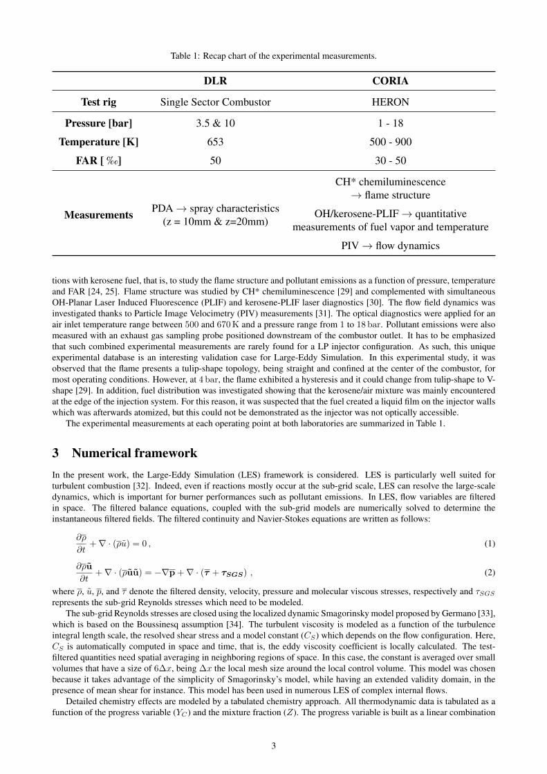
Table 1: Recap chart of the experimental measurements.

DLR CORIA

Test rig Single Sector Combustor HERON

Pressure [bar] 3.5 & 10 1 - 18

Temperature [K] 653 500 - 900

FAR [ ‰] 50 30 - 50

Measurements PDA→ spray characteristics(z = 10mm & z=20mm)

CH* chemiluminescence→ flame structure

OH/kerosene-PLIF→ quantitativemeasurements of fuel vapor and temperature

PIV→ flow dynamics

tions with kerosene fuel, that is, to study the flame structure and pollutant emissions as a function of pressure, temperatureand FAR [24, 25]. Flame structure was studied by CH* chemiluminescence [29] and complemented with simultaneousOH-Planar Laser Induced Fluorescence (PLIF) and kerosene-PLIF laser diagnostics [30]. The flow field dynamics wasinvestigated thanks to Particle Image Velocimetry (PIV) measurements [31]. The optical diagnostics were applied for anair inlet temperature range between 500 and 670 K and a pressure range from 1 to 18 bar. Pollutant emissions were alsomeasured with an exhaust gas sampling probe positioned downstream of the combustor outlet. It has to be emphasizedthat such combined experimental measurements are rarely found for a LP injector configuration. As such, this uniqueexperimental database is an interesting validation case for Large-Eddy Simulation. In this experimental study, it wasobserved that the flame presents a tulip-shape topology, being straight and confined at the center of the combustor, formost operating conditions. However, at 4 bar, the flame exhibited a hysteresis and it could change from tulip-shape to V-shape [29]. In addition, fuel distribution was investigated showing that the kerosene/air mixture was mainly encounteredat the edge of the injection system. For this reason, it was suspected that the fuel created a liquid film on the injector wallswhich was afterwards atomized, but this could not be demonstrated as the injector was not optically accessible.

The experimental measurements at each operating point at both laboratories are summarized in Table 1.

3 Numerical frameworkIn the present work, the Large-Eddy Simulation (LES) framework is considered. LES is particularly well suited forturbulent combustion [32]. Indeed, even if reactions mostly occur at the sub-grid scale, LES can resolve the large-scaledynamics, which is important for burner performances such as pollutant emissions. In LES, flow variables are filteredin space. The filtered balance equations, coupled with the sub-grid models are numerically solved to determine theinstantaneous filtered fields. The filtered continuity and Navier-Stokes equations are written as follows:

∂ρ

∂t+∇ · (ρu) = 0 , (1)

∂ρu

∂t+∇ · (ρuu) = −∇p +∇ · (τ + τSGS) , (2)

where ρ, u, p, and τ denote the filtered density, velocity, pressure and molecular viscous stresses, respectively and τSGSrepresents the sub-grid Reynolds stresses which need to be modeled.

The sub-grid Reynolds stresses are closed using the localized dynamic Smagorinsky model proposed by Germano [33],which is based on the Boussinesq assumption [34]. The turbulent viscosity is modeled as a function of the turbulenceintegral length scale, the resolved shear stress and a model constant (CS) which depends on the flow configuration. Here,CS is automatically computed in space and time, that is, the eddy viscosity coefficient is locally calculated. The test-filtered quantities need spatial averaging in neighboring regions of space. In this case, the constant is averaged over smallvolumes that have a size of 6∆x, being ∆x the local mesh size around the local control volume. This model was chosenbecause it takes advantage of the simplicity of Smagorinsky’s model, while having an extended validity domain, in thepresence of mean shear for instance. This model has been used in numerous LES of complex internal flows.

Detailed chemistry effects are modeled by a tabulated chemistry approach. All thermodynamic data is tabulated as afunction of the progress variable (YC) and the mixture fraction (Z). The progress variable is built as a linear combination

3

of species mass fractions (YC = YCO + YCO2 + YH2O) and allows to describe the progress of the reaction while Zcharacterizes the mixture, that is, it estimates the local equivalence ratio. Only these two parameters are transported withthe following equations:

∂ρYC∂t

+∇ · (ρYC u) = ∇ ·((ρD + ρDt,C

)∇YC

)+ ωYC

, (3)

and

∂ρZ

∂t+∇ · (ρZu) = ∇ ·

((ρD + ρDt,Z

)∇Z

)+ ωZ . (4)

In these equations, Dt,C and Dt,Z are the C and Z sub-grid transport fluxes, respectively, which are modeled with a con-stant turbulent Schmidt number (0.9). The source terms ωYC

and ωZ are due to chemistry and evaporation, respectively.To take into account the sub-grid flame-turbulence interaction the Presumed-Conditional Moments for Flame Prolonga-tion of ILDM (PCM-FPI) method is used [35]. The look-up table is built from laminar premixed flame archetypes to mapthe flame evolution. These flamelets are computed with Cantera [36] using the skeletal LUCHE mechanism [37], whichcounts 92 species and 694 reactions. Reaction rates and species mass fractions are tabulated as functions of YC and Z.This laminar look-up table is then convoluted by two beta Probability Density Functions (β-PDFs) [35, 38] to take intoaccount their sub-grid fluctuations. The β-PDF of the mixture fraction is defined for Z values from 0 to 1, even thoughit is known that the maximum value of the mixture fraction can not exceed the saturation value (Zsat < 1) when dealingwith two-phase flows. However, this approach can be valid as long as its variance is small enough, making the proportionof values above Zsat negligible [43]. The final look-up table is thus also parametrized by the second-order moments (Z ′′2,c′′2) of the beta-PDFs. These second-order moments are modeled by an algebraic approach based on the fact that thevariance presents asymptotic behaviors depending on the sub-filter scalar distribution [39]. The variance of the mixturefraction, which is well resolved on the considered meshes, is modeled as follows:

Z ′′2 = Cm∆2|∇Z|2 , (5)

where Cm is a constant equal to 0.08 and ∆ is the filter width. This model can be simply derived by neglecting anycurvature of the sub-filter mixture fraction and by performing a Taylor-series expansion of the filtering operators [39].However, this type of model can generally not be used for the progress variable, which is highly wrinkled at the sub-gridscale. In this case, a gradient model [40] for the sub-grid variance is prescribed:

c′′2 = Cg∆|∇c| , (6)

here Cg is the constant for the gradient model and is set to 0.18. This methodology has been chosen since there arenot many available kinetic schemes for kerosene capable of reproducing the characteristics of the flame at high pressureand temperature conditions and containing the required species for this study at a reasonable CPU cost. Besides, someprevious works such as [41, 42, 43] presented good results in the application of this methodology in spray flames.

3.1 Spray modelingIn many practical aeronautical applications, liquid fuel is injected into the combustion chamber resulting in fuel spray.The spray is a two-phase flow, which involves heat and mass transfer from the droplet phase to the continuous phasedue to vaporization. In combustion, the mass transfer is also accompanied by energy release and transport, which furtherenhances vaporization. This coupled nature of the transport phenomena makes spray combustion a problem that is bothinteresting and challenging to simulate [44].

In the present work, the Euler/Lagrange (EL) approach has been chosen to model the two-phase flow. The gas phaseis represented using the Eulerian description while the dispersed phase is represented by the Lagrangian frame. In thisapproach, quantities needed for the coupling between phases have to be interpolated at the droplet position or projected atthe mesh nodes [45].

It consists of the individual treatment of each droplet in the computational domain. Mass and heat transfer, momentumand energy apply between the two phases. Droplets have their own properties, i.e. temperature, diameter and velocity.The droplet motion is described by the following equations:

dxpdt

= up andmpdup

dt= FD + FG (7)

to describe its position (xp), its velocity (up) and the forces upon the droplet, where FD is the drag force [46] and FG

the gravity force. Gravity is neglected here as it is far smaller than the drag force. No droplet-droplet interactions areconsidered as the spray can be considered as diluted away from the primary atomization zone.

Moreover, the vaporization of the droplets is modeled using the Abramzon & Sirignano approach [47], which is anextension of the classical mass transfer model of Spalding [48]. Droplets are assumed to be spherical. For liquid drops,

4

sphericity is the result of predominant surface tension compared with the deformation effects of external stress, whoseratio is characterized by the Weber number [49]. A direct consequence of this assumption is that the droplet mass (mp)can be related to its diameter (dp). Thermodynamic properties of the droplet are obtained from the conservation equations.The evolution of the droplet’s mass is given by:

dmp

dt= −πdpSh(ρpD) log(1 +BM ) , (8)

where Sh is the Sherwood number [50], ρp is the droplet’s density, D is the thermal diffusivity, and BM the Spaldingnumber for the mass transfer [48]. Here ρp and D, depend on the temperature and the composition of the gas surroundingthe droplet. These properties may vary between the surface and the far field, for this reason, the “1/3-rule” [51] is applied.Temperature and species mass fraction in the reference state are obtained as:

Tref = Tsurf + 1/3(T∞ − Tsurf ) , (9)

Yk,ref = Yk,surf + 1/3(Yk,∞ − Yk,surf ) (10)

with T∞ and Yk,∞ the temperature and the species mass fraction in the far field, respectively and Tsurf and Yk,surf thetemperature and the species mass fraction at the surface of the droplet.

The droplet temperature (Tp) evolution is obtained by integrating the energy conservation from the droplet’s surfaceto the the far field, leading to,

dTpdt

= − 1

τh

[Tp −

(T∞ −

LvBTCp,ref

)], (11)

where τh is a thermal characteristic time, Lv the latent heat, BT the Spalding number for the heat transfer [48] and Cp,refis the reference heat capacity [43]. Besides, the variation of the mixture enthalpy due to the droplets vaporization can beconsidered negligible as the study is being done for a lean mixture and, hence, low equivalence ratios.

4 Numerical set-upSeveral LES of the HERON experimental facility equipped with the LP injection system are performed for one operatingpoint. Pressure in the combustion chamber is 8.33 bar and air is preheated at 669.3 K. An injector FAR of 42‰ hasbeen chosen. The air mass flow rate entering the combustion chamber is 108 g · s−1, which is split between the injectorand four lateral windows. These operating conditions have been motivated by the extended experimental characterizationof the flame and its good stability in these conditions even though it will be shown that the flame topology is extremelysensitive to the spray properties. Experimentally, the inlet ducts were insulated in order to preserve the temperatureconditions imposed at the inlet of the combustor and the air coming from the lateral windows helped to preserve thetemperature conditions inside the combustion chamber. For this reason, adiabatic boundary conditions are imposed. Themean Reynolds number, based on the diameter of the injector nozzle is about 192 000 and the entire domain flow-throughtime (τd) defined as the ratio between the length domain and the bulk velocity is around 5.33 ms.

As it was indicated in Sec. 2, the real process of atomization could not be captured experimentally. Here, this processis considered as a consequence of the high velocity of the air, leading to the so-called air-blast atomization [3]. In thiscase, the liquid jet momentum is small compared to the air momentum, hence, atomization is completely dependenton the momentum of the airflow. Besides, the droplets trajectories are dictated by the air movements created by theswirlers. Spray is then modeled as a cloud of droplets directly injected with a prescribed diameter PDF and a velocityprofile. This cloud of droplets is injected every time step in order to maintain the appropriate mass flow rate constant.Kerosene is modelled as a single-component fuel which has the same properties as the 3-component surrogate of theLuche mechanism [37]. In Table 2 the fuel parameters used in this work are summarized. Kerosene is injected intothe combustion chamber through holes. All of them have the same diameter, therefore the same amount of kerosene isinjected through each of the holes.

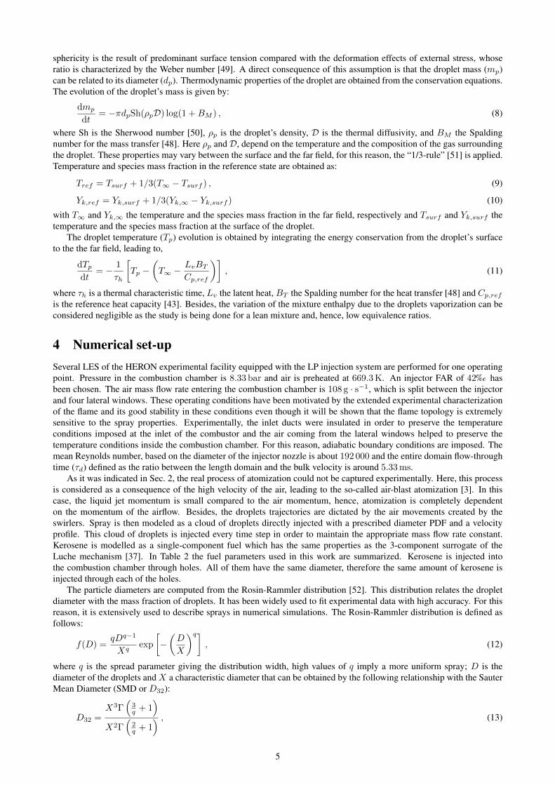
The particle diameters are computed from the Rosin-Rammler distribution [52]. This distribution relates the dropletdiameter with the mass fraction of droplets. It has been widely used to fit experimental data with high accuracy. For thisreason, it is extensively used to describe sprays in numerical simulations. The Rosin-Rammler distribution is defined asfollows:

f(D) =qDq−1

Xqexp

[−(D

X

)q], (12)

where q is the spread parameter giving the distribution width, high values of q imply a more uniform spray; D is thediameter of the droplets and X a characteristic diameter that can be obtained by the following relationship with the SauterMean Diameter (SMD or D32):

D32 =X3Γ

(3q + 1

)X2Γ

(2q + 1

) , (13)

5

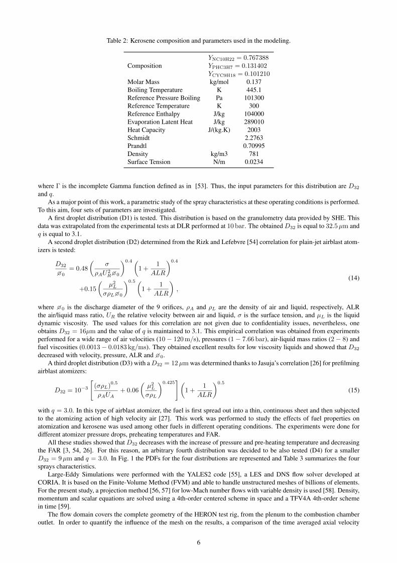
Table 2: Kerosene composition and parameters used in the modeling.

CompositionYNC10H22 = 0.767388YPHC3H7 = 0.131402YCYC9H18 = 0.101210

Molar Mass kg/mol 0.137Boiling Temperature K 445.1Reference Pressure Boiling Pa 101300Reference Temperature K 300Reference Enthalpy J/kg 104000Evaporation Latent Heat J/kg 289010Heat Capacity J/(kg.K) 2003Schmidt 2.2763Prandtl 0.70995Density kg/m3 781Surface Tension N/m 0.0234

where Γ is the incomplete Gamma function defined as in [53]. Thus, the input parameters for this distribution are D32

and q.As a major point of this work, a parametric study of the spray characteristics at these operating conditions is performed.

To this aim, four sets of parameters are investigated.A first droplet distribution (D1) is tested. This distribution is based on the granulometry data provided by SHE. This

data was extrapolated from the experimental tests at DLR performed at 10 bar. The obtained D32 is equal to 32.5µm andq is equal to 3.1.

A second droplet distribution (D2) determined from the Rizk and Lefebvre [54] correlation for plain-jet airblast atom-izers is tested:

D32

�0= 0.48

(σ

ρAU2R�0

)0.4(1 +

1

ALR

)0.4

+0.15

(µ2L

σρL�0

)0.5(1 +

1

ALR

),

(14)

where �0 is the discharge diameter of the 9 orifices, ρA and ρL are the density of air and liquid, respectively, ALRthe air/liquid mass ratio, UR the relative velocity between air and liquid, σ is the surface tension, and µL is the liquiddynamic viscosity. The used values for this correlation are not given due to confidentiality issues, nevertheless, oneobtains D32 = 16µm and the value of q is maintained to 3.1. This empirical correlation was obtained from experimentsperformed for a wide range of air velocities (10 − 120 m/s), pressures (1 − 7.66 bar), air-liquid mass ratios (2 − 8) andfuel viscosities (0.0013− 0.0183 kg/ms). They obtained excellent results for low viscosity liquids and showed that D32

decreased with velocity, pressure, ALR and �0.A third droplet distribution (D3) with aD32 = 12µm was determined thanks to Jasuja’s correlation [26] for prefilming

airblast atomizers:

D32 = 10−3

[(σρL)

0.5

ρAUA+ 0.06

(µ2L

σρL

)0.425](

1 +1

ALR

)0.5

(15)

with q = 3.0. In this type of airblast atomizer, the fuel is first spread out into a thin, continuous sheet and then subjectedto the atomizing action of high velocity air [27]. This work was performed to study the effects of fuel properties onatomization and kerosene was used among other fuels in different operating conditions. The experiments were done fordifferent atomizer pressure drops, preheating temperatures and FAR.

All these studies showed that D32 decreases with the increase of pressure and pre-heating temperature and decreasingthe FAR [3, 54, 26]. For this reason, an arbitrary fourth distribution was decided to be also tested (D4) for a smallerD32 = 9µm and q = 3.0. In Fig. 1 the PDFs for the four distributions are represented and Table 3 summarizes the foursprays characteristics.

Large-Eddy Simulations were performed with the YALES2 code [55], a LES and DNS flow solver developed atCORIA. It is based on the Finite-Volume Method (FVM) and able to handle unstructured meshes of billions of elements.For the present study, a projection method [56, 57] for low-Mach number flows with variable density is used [58]. Density,momentum and scalar equations are solved using a 4th-order centered scheme in space and a TFV4A 4th-order schemein time [59].

The flow domain covers the complete geometry of the HERON test rig, from the plenum to the combustion chamberoutlet. In order to quantify the influence of the mesh on the results, a comparison of the time averaged axial velocity

6

0 10 20 30 40 50 60Diameter [µm]

0.00

0.02

0.04

0.06

0.08

0.10

0.12

0.14P

DF

[−]

D1

D2

D3

D4

Figure 1: Rosin-Rammler PDFs distributions

Table 3: Spray parametric study.

D1 D2 D3 D4

D32 [µm] 32.5 16 12 09

q 3.1 3.1 3.0 3.0

Source SHE Rizk andLefebvre [54] Jasuja [26] CORIA

7

−20 0 20 40 60 80−2.0

−1.5

−1.0

−0.5

0.0

0.5

1.0

1.5

2.0

x/D

[-]

z/D = 0.34

−20 0 20 40 60 80

z/D = 0.50

−20 0 20 40 60 80

〈Uaxial〉 [m · s−1]

z/D = 0.74

−20 0 20 40 60 80

z/D = 0.93

−20 0 20 40 60

z/D = 1.37

30M el 237M el

Figure 2: Axial velocity comparison for two different meshes with experimental results for distribution D3

Figure 3: Cell size of the flow domain

with experimental data is presented in Fig. 2 for two different meshes. This comparison was done in reacting conditions,since it was observed that spray influences the aerodynamics of the flow field. Only the comparison for distribution D3is presented for more clarity. The first mesh consists of around 30 million elements, while the second one is a refinementof the first one and has around 237 million elements. In these curves it can be seen that by refining the mesh the resultsare more accurate with respect to the experimental results. No other refinement level was performed as its cost would beprohibitive.

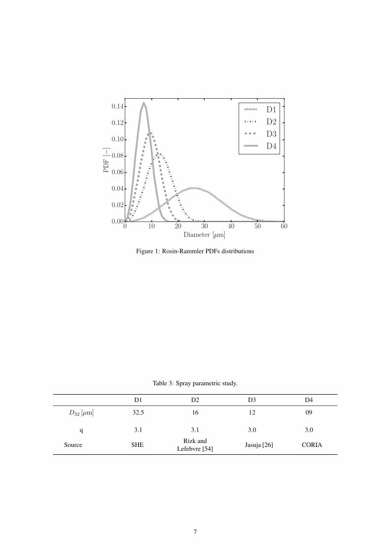
In Fig. 3 some details on the mesh size are presented. In the injection and flame zone, a refined area is defined by acone. Here, the largest elements have a size of 0.25 mm and the flame thickness at this operating conditions is around0.074 mm. The lateral windows discretization is challenging as they are cooled by a thin film of air. They are thusdiscretized by small cells with a maximal size of 0.15 mm, which allows for having at least seven cells in the film. Themesh resolution on the wall can be evaluated thanks to the dimensionless wall distance, y+. Fig. 4 shows the PDF of they+ values in the injector wall, which is the most critical area. It can be seen that the highest values of y+ are about 50,although the distribution shows that most of its values are around 10. To the authors’ experience injector walls can beconsidered sufficiently resolved to capture the correct flow field and pressure drop in the injector with no slip boundaryconditions.

In order to bring more insights in the mesh resolution, Fig. 5 represents the ratio of the cell size (∆) and the Kol-mogorovas length scale (ηK). In Fig. 5(a), a general overview of this ratio together with its PDF in Fig. 5(b) are repre-sented. In Fig. 5(c), only the refined cone is shown with the flame zone framed by an iso-contour of the time averaged

8

Figure 4: PDF of the y+ values in the injector wall for distribution D1, D2, D3 and D4

temperature (〈T〉 = 1500 K). It can be seen that despite some cells present a big ratio, most of the cells in the zone ofinterest, have a ratio around 10. Here, the Kolmogorov’s length scale is computed as [39]:

ηK =

(ν3

ε

)(1/4)

(16)

where

ε = Cεk3/2sgs

∆with ksgs =

(νT

C(1/3)ε C

(4/3)S ∆

)2

, (17)

being, ε the sub-grid dissipation, ksgs the sub-grid kinetic energy, Cε ≈ 1.05, CS the dynamic Smagorinsky constantand νT the sub-grid eddy viscosity.

In Table 4, the accumulated times for each distribution as well as the computer resources used to perform these simu-lations are summarized. Data can be considered converged since at least 10 flow-through times passed before starting thecollection of statistics. Besides, the statistics were also collected during several flow-though times. Despite that accumu-lated times for distribution D2 and D4 are smaller than times for D1 and D3, it should be noted that these computationswere not started from the beginning but from computation D2 when the flow field was already converged. The compu-tational cost considerably increases with decreasing the droplet size. This is due to the fact that with the same injectedkerosene mass flow rate more droplets must be injected with smaller diameters. To palliate the problem of injecting ahuge amount of droplets, a numerical parcel approach has been employed, where one numerical parcel is equivalent toten droplets sharing the same location and other properties (velocity, temperature, . . . ). Although for distribution D1the particle cost is not excessively high, the same approach was decided to be used in order to keep the same modelingapproach in all computations.

5 Results and discussion

5.1 Aerodynamic flow fieldThe analysis of the flow field in Fig. 6 is represented by the instantaneous (above) and the time-averaged (below) axialvelocity fields. The shape, size and position of the two recirculation zones can be identified thanks to the zero axialvelocity iso-lines. These recirculation zones, characteristic of swirled flows, are the Central Recirculation Zone (CRZ)and the Outer Recirculation Zone (ORZ). Both recirculation zones are important, since they contribute to bringing burntgases towards the injection zone helping in stabilizing the flame. The CRZ usually acts as an aerodynamic flame holdersince it creates low velocity regions where the flame can anchor [60, 61] and can affect the position of the flame. Itcan be seen that for distribution D1 (Fig. 6(a)), the CRZ is larger and more elongated. Here, the CRZ starts inside theinjector, being very narrow initially and then thickening mainly in the combustion chamber. For distributions D2 and D3

9

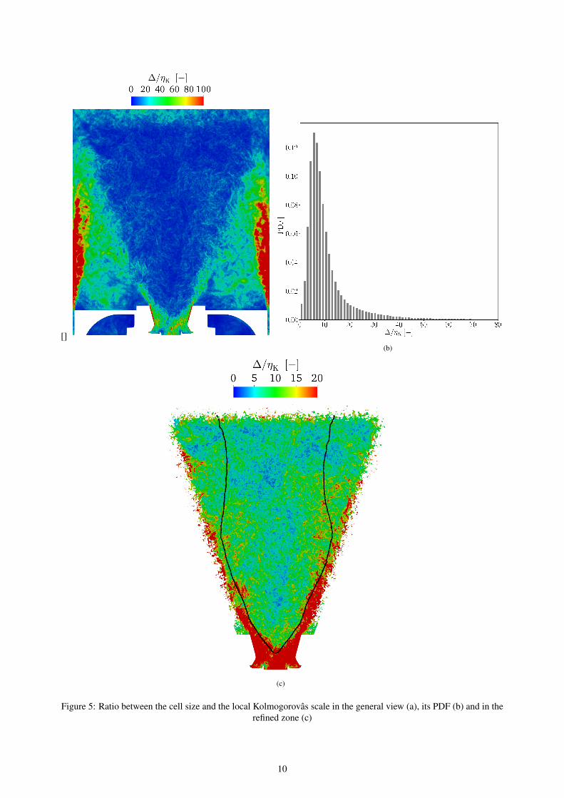
[](b)

(c)

Figure 5: Ratio between the cell size and the local Kolmogorovas scale in the general view (a), its PDF (b) and in therefined zone (c)

10

Table 4: Summary of accumulated times and performances for each distribution.

D1 D2 D3 D4

Cumulated physical time[ms] 215 50 110 55

Physical flow-through timesproportion (τd = 5.33 ms) 44.33 τd 9.38 τd 20.63 τd 10.3 τd

Statistics cumulated time[ms] 60 25 58 38

Statistics flow-throughtimes proportion (τd = 5.33

ms)11.2 τd 4.7 τd 10.88 τd 7.13 τd

Averaged injected particlesper time-step 39155 176928 416420 966568

Computational cost [%] 5.6 15.75 47.78 63.33

Computer center Occigen Occigen Myria Occigen

ProcessorIntel XeonBroadwell(2.6 GHz)

Intel XeonBroadwell(2.6 GHz)

Intel XeonBroadwell(2.2 GHz)

Intel XeonBroadwell(2.6 GHz)

# Processors 448 448 896 896

Physical time in 20 hours[ms] 1.00 0.90 0.75 0.50

11

Figure 6: Mid-plane instantaneous (above) and time-averaged (below) axial velocity fields with iso-lines (in white) ofzero-axial velocity representing recirculation zones for distribution D1 (a), D2 (b), D3 (c) and D4 (d)

12

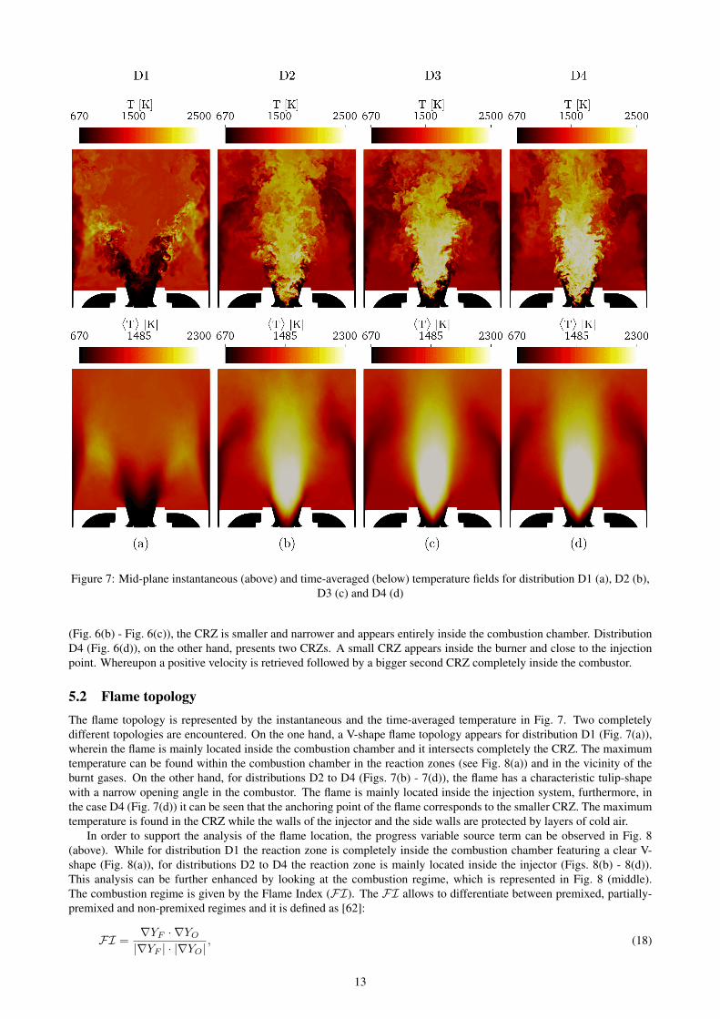
Figure 7: Mid-plane instantaneous (above) and time-averaged (below) temperature fields for distribution D1 (a), D2 (b),D3 (c) and D4 (d)

(Fig. 6(b) - Fig. 6(c)), the CRZ is smaller and narrower and appears entirely inside the combustion chamber. DistributionD4 (Fig. 6(d)), on the other hand, presents two CRZs. A small CRZ appears inside the burner and close to the injectionpoint. Whereupon a positive velocity is retrieved followed by a bigger second CRZ completely inside the combustor.

5.2 Flame topologyThe flame topology is represented by the instantaneous and the time-averaged temperature in Fig. 7. Two completelydifferent topologies are encountered. On the one hand, a V-shape flame topology appears for distribution D1 (Fig. 7(a)),wherein the flame is mainly located inside the combustion chamber and it intersects completely the CRZ. The maximumtemperature can be found within the combustion chamber in the reaction zones (see Fig. 8(a)) and in the vicinity of theburnt gases. On the other hand, for distributions D2 to D4 (Figs. 7(b) - 7(d)), the flame has a characteristic tulip-shapewith a narrow opening angle in the combustor. The flame is mainly located inside the injection system, furthermore, inthe case D4 (Fig. 7(d)) it can be seen that the anchoring point of the flame corresponds to the smaller CRZ. The maximumtemperature is found in the CRZ while the walls of the injector and the side walls are protected by layers of cold air.

In order to support the analysis of the flame location, the progress variable source term can be observed in Fig. 8(above). While for distribution D1 the reaction zone is completely inside the combustion chamber featuring a clear V-shape (Fig. 8(a)), for distributions D2 to D4 the reaction zone is mainly located inside the injector (Figs. 8(b) - 8(d)).This analysis can be further enhanced by looking at the combustion regime, which is represented in Fig. 8 (middle).The combustion regime is given by the Flame Index (FI). The FI allows to differentiate between premixed, partially-premixed and non-premixed regimes and it is defined as [62]:

FI =∇YF · ∇YO|∇YF | · |∇YO|

, (18)

13

(a) (b) (c) (d)

Figure 8: Midplane of the time-averaged reaction rate (above), the combustion regime in the reaction zone representedby the surface rendering of the flame index conditioned by the source term of the progress variable (middle):

non-premixed ( ), premixed ( ) and partially premixed ( ) and the PDFs of the flame index (below) for D1 (a), D2 (b),D3 (c) and D4 (d)

14

where YF is the fuel mass fraction and YO the oxidant mass fraction. This index is equal to FI = 1 for premixedcombustion regimes, represented by golden-colored iso-surface and FI = −1 for non-premixed regimes, represented byblack-colored iso-surface. All intermediate values correspond to partially premixed zones, represented by the purple iso-surface. TheFI representation is conditioned by the instantaneous field of the progress variable source term. Combustionoccurs mostly in premixed and partially premixed regimes for distribution D1 (Fig. 8(a)). This is because the evaporatedkerosene along the injector has enough time to mix with air before burning. By contrast, for the other three distributions,a non-premixed combustion regime can be encountered very close to the injection point. Here, as fuel and air are injectedseparately, kerosene has not yet been able to mix with fresh gases before reaching the reaction zone. However, it changesrapidly to premixed regime still inside the injector due to the mixing with the fresh and burnt gases brought in by theCRZ. Then, further downstream, moving on through the combustion chamber the fuel mixes with the air flow from theouter swirler and the partially premixed combustion regime is predominant. Finally, the PDFs of the flame index in Fig. 8(below) allow to confirm the preceding evaluation of the combustion regime. It can be seen that while for distribution D1(Fig. 8(a)), the PDF shows a primacy of the premixed and partially premixed regimes, the other three distributions aremore balanced between all three combustion regimes (Fig. 8(b) - 8(d)). The combustion regimes inside the injector aretherefore very complex and challenging to capture.

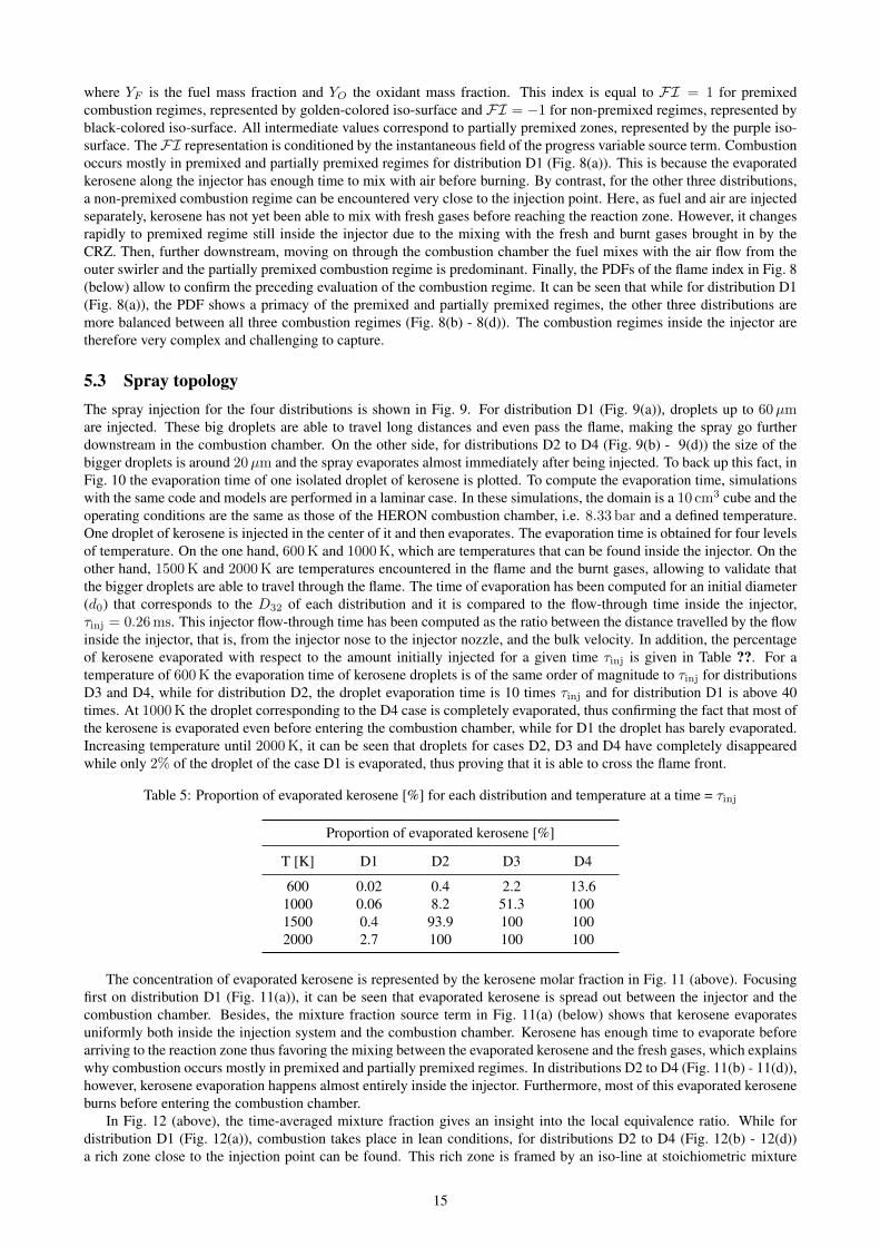
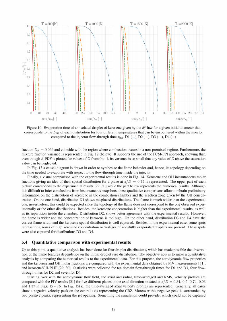
5.3 Spray topologyThe spray injection for the four distributions is shown in Fig. 9. For distribution D1 (Fig. 9(a)), droplets up to 60µmare injected. These big droplets are able to travel long distances and even pass the flame, making the spray go furtherdownstream in the combustion chamber. On the other side, for distributions D2 to D4 (Fig. 9(b) - 9(d)) the size of thebigger droplets is around 20µm and the spray evaporates almost immediately after being injected. To back up this fact, inFig. 10 the evaporation time of one isolated droplet of kerosene is plotted. To compute the evaporation time, simulationswith the same code and models are performed in a laminar case. In these simulations, the domain is a 10 cm3 cube and theoperating conditions are the same as those of the HERON combustion chamber, i.e. 8.33 bar and a defined temperature.One droplet of kerosene is injected in the center of it and then evaporates. The evaporation time is obtained for four levelsof temperature. On the one hand, 600 K and 1000 K, which are temperatures that can be found inside the injector. On theother hand, 1500 K and 2000 K are temperatures encountered in the flame and the burnt gases, allowing to validate thatthe bigger droplets are able to travel through the flame. The time of evaporation has been computed for an initial diameter(d0) that corresponds to the D32 of each distribution and it is compared to the flow-through time inside the injector,τinj = 0.26 ms. This injector flow-through time has been computed as the ratio between the distance travelled by the flowinside the injector, that is, from the injector nose to the injector nozzle, and the bulk velocity. In addition, the percentageof kerosene evaporated with respect to the amount initially injected for a given time τinj is given in Table ??. For atemperature of 600 K the evaporation time of kerosene droplets is of the same order of magnitude to τinj for distributionsD3 and D4, while for distribution D2, the droplet evaporation time is 10 times τinj and for distribution D1 is above 40times. At 1000 K the droplet corresponding to the D4 case is completely evaporated, thus confirming the fact that most ofthe kerosene is evaporated even before entering the combustion chamber, while for D1 the droplet has barely evaporated.Increasing temperature until 2000 K, it can be seen that droplets for cases D2, D3 and D4 have completely disappearedwhile only 2% of the droplet of the case D1 is evaporated, thus proving that it is able to cross the flame front.

Table 5: Proportion of evaporated kerosene [%] for each distribution and temperature at a time = τinj

Proportion of evaporated kerosene [%]

T [K] D1 D2 D3 D4

600 0.02 0.4 2.2 13.61000 0.06 8.2 51.3 1001500 0.4 93.9 100 1002000 2.7 100 100 100

The concentration of evaporated kerosene is represented by the kerosene molar fraction in Fig. 11 (above). Focusingfirst on distribution D1 (Fig. 11(a)), it can be seen that evaporated kerosene is spread out between the injector and thecombustion chamber. Besides, the mixture fraction source term in Fig. 11(a) (below) shows that kerosene evaporatesuniformly both inside the injection system and the combustion chamber. Kerosene has enough time to evaporate beforearriving to the reaction zone thus favoring the mixing between the evaporated kerosene and the fresh gases, which explainswhy combustion occurs mostly in premixed and partially premixed regimes. In distributions D2 to D4 (Fig. 11(b) - 11(d)),however, kerosene evaporation happens almost entirely inside the injector. Furthermore, most of this evaporated keroseneburns before entering the combustion chamber.

In Fig. 12 (above), the time-averaged mixture fraction gives an insight into the local equivalence ratio. While fordistribution D1 (Fig. 12(a)), combustion takes place in lean conditions, for distributions D2 to D4 (Fig. 12(b) - 12(d))a rich zone close to the injection point can be found. This rich zone is framed by an iso-line at stoichiometric mixture

15

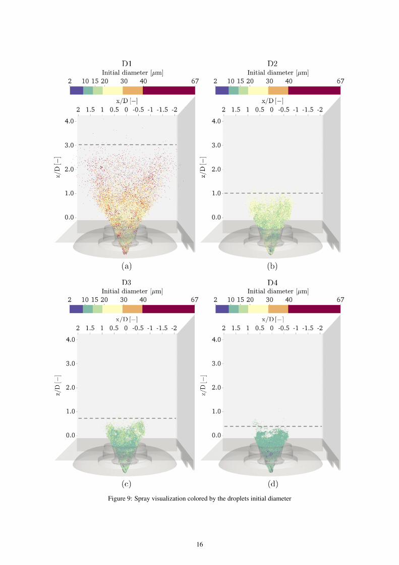
Figure 9: Spray visualization colored by the droplets initial diameter

16

0 10 20 30 40

time/τinj [−]

0.1

0.2

0.3

0.4

0.5

0.6

0.7

0.8

0.9

1.0(d/d

0)2

[−]

T =600 [K]

0.0 2.5 5.0 7.5 10.0 12.5

time/τinj [−]

T =1000 [K]

0 1 2 3 4

time/τinj [−]

T =1500 [K]

0.0 0.5 1.0 1.5 2.0 2.5 3.0

time/τinj [−]

T =2000 [K]

Figure 10: Evaporation time of an isolated droplet of kerosene given by the d2-law for a given initial diameter thatcorresponds to the D32 of each distribution for four different temperatures that can be encountered within the injector

compared to the injector flow-through time τinj. D1 ( ), D2 ( ), D3 ( ), D4 ( )

fraction Zst = 0.066 and coincide with the region where combustion occurs in a non-premixed regime. Furthermore, themixture fraction variance is represented in Fig. 12 (below). It supports the use of the PCM-FPI approach, showing that,even though β-PDF is plotted for values of Z from 0 to 1, its variance is so small that any value of Z above the saturationvalue can be neglected.

In Fig. 13 a causal diagram is drawn in order to synthesize the flame behavior and, hence, its topology depending onthe time needed to evaporate with respect to the flow-through time inside the injector.

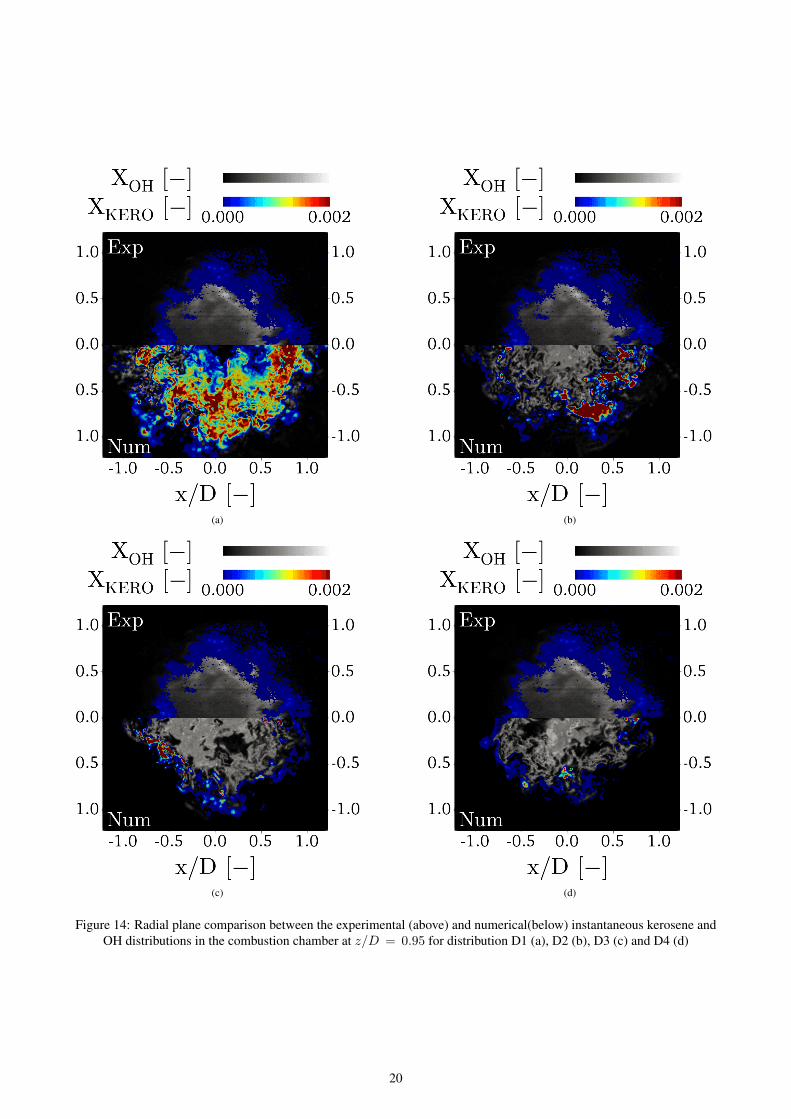
Finally, a visual comparison with the experimental results is done in Fig. 14. Kerosene and OH instantaneous molarfractions giving an idea of their spatial distribution for a plane at z/D = 0.75 is represented. The upper part of eachpicture corresponds to the experimental results [29, 30] while the part below represents the numerical results. Althoughit is difficult to infer conclusions from instantaneous snapshots, these qualitative comparisons allow to obtain preliminaryinformation on the distribution of kerosene in the combustion chamber and the reaction zone given by the OH concen-tration. On the one hand, distribution D1 shows misplaced distributions. The flame is much wider than the experimentalone, nevertheless, this could be expected since the topology of the flame does not correspond to the one observed exper-imentally or the other distributions. Besides, the kerosene concentration is higher than the experimental results, as wellas its repartition inside the chamber. Distribution D2, shows better agreement with the experimental results. However,the flame is wider and the concentration of kerosene is too high. On the other hand, distribution D3 and D4 have thecorrect flame width and the kerosene spatial distribution is well captured. Besides, in the experimental case, some spotsrepresenting zones of high kerosene concentration or vestiges of non-fully evaporated droplets are present. These spotswere also captured for distributions D3 and D4.

5.4 Quantitative comparison with experimental resultsUp to this point, a qualitative analysis has been done for four droplet distributions, which has made possible the observa-tion of the flame features dependence on the initial droplet size distribution. The objective now is to make a quantitativeanalysis by comparing the numerical results to the experimental data. For this purpose, the aerodynamic flow propertiesand the kerosene and OH molar fractions are compared with the experimental data obtained by PIV measurements [31],and kerosene/OH-PLIF [29, 30]. Statistics were collected for ten domain flow-through times for D1 and D3, four flow-through times for D2 and seven for D4.

Starting over with the aerodynamic flow field, the axial and radial, time-averaged and RMS, velocity profiles arecompared with the PIV results [31] for five different planes in the axial direction situated at z/D = 0.34, 0.5, 0.74, 0.93and 1.37 in Figs. 15 - 16. In Fig. 15(a), the time-averaged axial velocity profiles are represented. Generally, all casesshow a negative velocity peak on the central axis representing the CRZ. Moreover this negative peak is surrounded bytwo positive peaks, representing the jet opening. Something the simulation could provide, which could not be captured

17

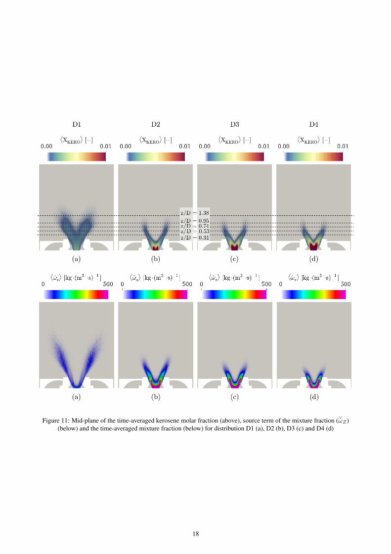
Figure 11: Mid-plane of the time-averaged kerosene molar fraction (above), source term of the mixture fraction (ωZ)(below) and the time-averaged mixture fraction (below) for distribution D1 (a), D2 (b), D3 (c) and D4 (d)

18

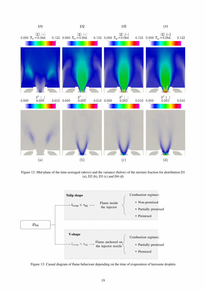
Figure 12: Mid-plane of the time-averaged (above) and the variance (below) of the mixture fraction for distribution D1(a), D2 (b), D3 (c) and D4 (d)

D32

tevap < τinjtevap < τinjFlame insidethe injector

Combustion regimes:

• Non-premixed

• Partially premixed

• Premixed

Tulip shape

tevap > τinjFlame anchored onthe injector nozzle

Combustion regimes:

• Partially premixed

• Premixed

V-shape

Figure 13: Casual diagram of flame behaviour depending on the time of evaporation of kerosene droplets

19

(a) (b)

(c) (d)

Figure 14: Radial plane comparison between the experimental (above) and numerical(below) instantaneous kerosene andOH distributions in the combustion chamber at z/D = 0.95 for distribution D1 (a), D2 (b), D3 (c) and D4 (d)

20

−20 0 20 40 60 80−2.0

−1.5

−1.0

−0.5

0.0

0.5

1.0

1.5

2.0x/

D[-

]z/D = 0.34

−20 0 20 40 60 80

z/D = 0.50

−20 0 20 40 60 80

〈Uaxial〉 [m · s−1]

z/D = 0.74

−20 0 20 40 60 80

z/D = 0.93

−20 0 20 40 60

z/D = 1.37

(a)

0 10 20−2.0

−1.5

−1.0

−0.5

0.0

0.5

1.0

1.5

2.0

x/D

[-]

z/D = 0.34

0 10 20

z/D = 0.50

0 10 20

URMSaxial [m · s−1]

z/D = 0.74

0 10 20

z/D = 0.93

0 10 20

z/D = 1.37

(b)

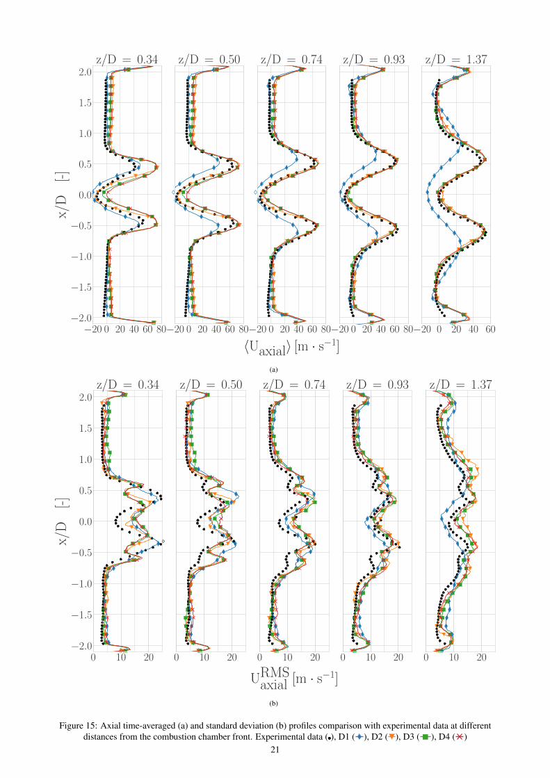
Figure 15: Axial time-averaged (a) and standard deviation (b) profiles comparison with experimental data at differentdistances from the combustion chamber front. Experimental data ( ), D1 ( ), D2 ( ), D3 ( ), D4 ( )

21

−20−10 0 10 20−2.0

−1.5

−1.0

−0.5

0.0

0.5

1.0

1.5

2.0x/

D[-

]z/D = 0.34

−20−10 0 10 20

z/D = 0.50

−20−10 0 10 20

〈Uradial〉 [m · s−1]

z/D = 0.74

−20−10 0 10 20

z/D = 0.93

−20−10 0 10 20

z/D = 1.37

(a)

0 10 20−2.0

−1.5

−1.0

−0.5

0.0

0.5

1.0

1.5

2.0

x/D

[-]

z/D = 0.34

0 10 20

z/D = 0.50

0 10 20

URMSradial [m · s−1]

z/D = 0.74

0 10 20

z/D = 0.93

0 10 20

z/D = 1.37

(b)

Figure 16: Radial time-averaged (a) and standard deviation (b) profiles comparison with experimental data at differentdistances from the combustion chamber front. Experimental data ( ), D1 ( ), D2 ( ), D3 ( ), D4 ( )

22

0.0 0.5 1.0 1.5×10−3

−1.00

−0.75

−0.50

−0.25

0.00

0.25

0.50

0.75

1.00x/

D[-

]z/D = 0.31

0.0 0.5 1.0 1.5×10−3

z/D = 0.53

0.0 0.5 1.0 1.5

〈XKERO〉 [-]×10−3

z/D = 0.74

0.0 0.5 1.0 1.5×10−3

z/D = 0.95

0.0 0.5 1.0 1.5×10−3

z/D = 1.38

(a)

0 1 2 3 4×10−3

−1.00

−0.75

−0.50

−0.25

0.00

0.25

0.50

0.75

1.00

x/D

[-]

z/D = 0.31

0 1 2 3 4×10−3

z/D = 0.53

0 1 2 3 4

〈XOH〉 [-]×10−3

z/D = 0.74

0 1 2 3 4×10−3

z/D = 0.95

0 1 2 3 4×10−3

z/D = 1.38

(b)

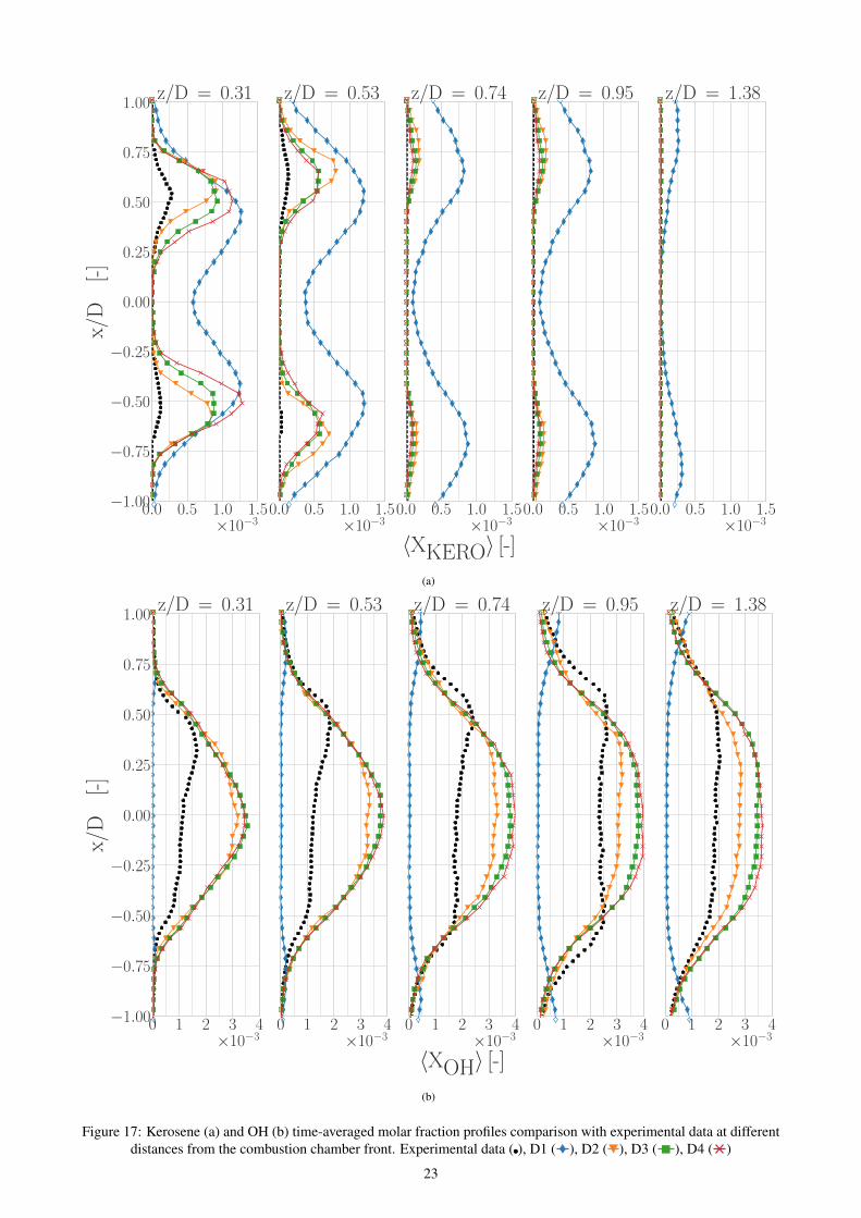
Figure 17: Kerosene (a) and OH (b) time-averaged molar fraction profiles comparison with experimental data at differentdistances from the combustion chamber front. Experimental data ( ), D1 ( ), D2 ( ), D3 ( ), D4 ( )

23

0.000 0.025 0.050 0.075 0.100 0.125 0.150 0.175YC [−]

0.0000

0.0005

0.0010

0.0015

0.0020

0.0025

YO

H[−

]

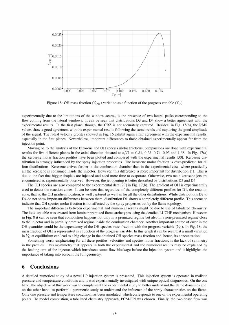
Figure 18: OH mass fraction (YOH ) variation as a function of the progress variable (YC)

experimentally due to the limitations of the window access, is the presence of two lateral peaks corresponding to theflow coming from the lateral windows. It can be seen that distributions D3 and D4 show a better agreement with theexperimental results. In the first plane, though, the CRZ is not accurately captured. Besides, in Fig. 15(b), the RMSvalues show a good agreement with the experimental results following the same trends and capturing the good amplitudeof the signal. The radial velocity profiles showed in Fig. 16 exhibit again a fair agreement with the experimental results,especially in the first planes. Nevertheless, important differences to those obtained experimentally appear far from theinjection point.

Moving on to the analysis of the kerosene and OH species molar fractions, comparisons are done with experimentalresults for five different planes in the axial direction situated at z/D = 0.31, 0.53, 0.74, 0.95 and 1.38. In Fig. 17(a)the kerosene molar fraction profiles have been plotted and compared with the experimental results [30]. Kerosene dis-tribution is strongly influenced by the spray injection properties. The kerosene molar fraction is over-predicted for allfour distributions. Kerosene arrives farther in the combustion chamber than in the experimental case, where practicallyall the kerosene is consumed inside the injector. However, this difference is more important for distribution D1. This isdue to the fact that bigger droplets are injected and need more time to evaporate. Otherwise, two main kerosene jets areencountered as experimentally observed. However, the jet opening is better described by distributions D3 and D4.

The OH species are also compared to the experimental data [29] in Fig. 17(b). The gradient of OH is experimentallyused to detect the reaction zones. It can be seen that regardless of the completely different profiles for D1, the reactionzone, that is, the OH gradient location, is well captured as well as for all the other distributions. While distributions D2 toD4 do not show important differences between them, distribution D1 shows a completely different profile. This seems toindicate that OH species molar fraction is not affected by the spray properties but by the flame topology.

The important differences between experimental and numerical results might be due to use of tabulated chemistry.The look-up table was created from laminar premixed flame archetypes using the detailed LUCHE mechanism. However,in Fig. 8 it can be seen that combustion happens not only in a premixed regime but also in a non-premixed regime closeto the injector and in partially premixed regime inside the combustion chamber. Another important source of error in theOH quantities could be the dependency of the OH species mass fraction with the progress variable (YC). In Fig. 18, themass fraction of OH is represented as a function of the progress variable. In this graph it can be seen that a small variationin YC at equilibrium can lead to a big change in the obtained OH species mass fraction and, hence, its concentration.

Something worth emphasizing for all these profiles, velocities and species molar fractions, is the lack of symmetryin the profiles. This asymmetry that appears in both the experimental and the numerical results may be explained bythe feeding arm of the injector which introduces some flow blockage before the injection system and it highlights theimportance of taking into account the full geometry.

6 ConclusionsA detailed numerical study of a novel LP injection system is presented. This injection system is operated in realisticpressure and temperature conditions and it was experimentally investigated with unique optical diagnostics. On the onehand, the objective of this work was to complement the experimental study to better understand the flame dynamics and,on the other hand, to perform a parametric study to understand the influence of the spray characteristics on the flame.Only one pressure and temperature condition has been simulated, which corresponds to one of the experimental operatingpoints. To model combustion, a tabulated chemistry approach, PCM-FPI was chosen. Finally, the two-phase flow was

24

described by a Euler-Lagrangian approach.Results have shown that flow aerodynamics is slightly influenced by the initial spray parameters. All distributions

present the two recirculation zones characteristics of swirled flames which contribute to stabilizing the flame.The flame and the spray topologies are strongly affected by the spray initial characteristics. It has been observed that

flame can present two different topologies, V-shape or tulip-shape, and that this is completely dependent on the qualityof the atomization. On the one hand, in the V-shape case, the flame is localized inside the combustor and the maximumtemperatures can be found in the reaction zones and around the burnt gases. Combustion, lean all over the combustor,happens mostly in premixed and partially premixed regime. This behavior is directly related with the spray features.Kerosene arrives further downstream and evaporation occurs in a more widespread manner which favors the mixingbetween fuel and air. On the other hand, the tulip-shape flame is mainly localized inside the injector and the maximumtemperature regions are found inside the CRZ. Here, the three combustion regimes can be encountered. Combustionregime starts being non-premixed close to the injection point, where it happens to be fuel-rich. It turns to premixed regimein the CRZ, where it mixes with burnt gases and it finally changes to partially-premixed regime inside the combustionchamber. In this case, kerosene evaporates very fast once it is injected and only the bigger droplets enter the combustor.

Furthermore, a quantitative analysis has made possible to compare the axial and radial velocities and the keroseneand OH species concentrations with the experimental data. On one hand, the axial and radial time-averaged and RMShave been compared to PIV measurements for five planes. The CRZ is well captured as well as the jet width and theasymmetry of the profiles. Quantitatively, the aerodynamics of the flow are barely influenced by the spray characteristics.On the other hand, the kerosene and OH species time-averaged molar fractions have been compared with kerosene/OH-PLIF measurements. Evaporated kerosene is broadly over-predicted for all four distributions, specially in the near-planesof the injector nozzle. This excess of evaporated kerosene is more evident for distribution D1, since in experiments nokerosene is left downstream on the combustion chamber. The OH profiles capture correctly the gradient location, that is,the reaction zone. However, there is an over-prediction of the OH concentration which may be due to the use of tabulatedchemistry combined with the evaporation models.

To summarize, it has been observed that spray modeling is decisive to obtain the good behavior of the flame and thatthe droplets evaporation time is directly related with the flame topology. It may affect not only the flame topology andits anchoring point, but also the combustion regime and the species spatial distribution. This study further highlights theimportance of atomization performances in the LP injection design.

The experimental database will be extended by granulometry measurements, allowing us to compare this parametricstudy with the real droplet size distribution.

AcknowledgementsThe authors thank the experimental team, Pierre Malbois, Erwan Salaun and Felix Frindt, who provided their insights andexpertise. This work was funded by ANR / SAFRAN / INSA Rouen / CNRS / ONERA in the framework of the industrialchair PERCEVAL and the experimental tests were funded by SAFRAN Helicopter Engines through GENOME programof the Direction Generale de l’Aviation Civile (DGAC) . It was granted access to the HPC resources from CINES underthe allocations x20172b6880 made by GENCI. It was also granted CPU time by CRIANN under the allocation 2012006.

References[1] European Aeronautics: A vision for 2020, 26.

[2] Huang Y., Vigor Y., Dynamics and stability of lean-premixed swirl-stabilized combustion, Progress in Energy andCombustion Science, 35, 293–364 (2009).

[3] Lefebvre A.H., Properties of sprays (1989).

[4] Ma R., Dong B., Yu Z., Zhang T., Wang Y., Li W., An experimental study on the spray characteristics of the air-blastatomizer, Applied Thermal Engineering, 88, 149–156 (2015).

[5] Gad H. M., Ibrahim I. A., Abdel-baky M. E., Abd El-samed A. K., Farag T. M., Experimental study of diesel fuelatomization performance of air blast atomizer, 99, 211–218 (2018).

[6] Urban A., Zaremba M., Maly M., Jozsa V., Jedelsky J., Droplet dynamics and size characterization of high-velocityairblast atomization, International Journal of Multiphase Flow, 95, 1–11 (2017).

[7] Garcıa M., Sommerer Y., Schonfeld T., Poinsot T., Assessment of Euler-Euler and Euler-Lagrange Strategies forReactive Large-Eddy Simulations, in: CERFACS - IMFT, 11 (2004).

[8] Patel N., Menon S., Simulation of spray-turbulence-flame interactions in a lean direct injection combustor, Combus-tion and Flame, 153, 228–257 (2008).

25

[9] Apte S. V., Mahesh K., Moin P., Oefelein J. C., Large-eddy simulation of swirling particle-laden flows in a coaxial-jetcombustor, International Journal of Multiphase Flow, 29, 1311–1331 (2003).

[10] Yoo Y., Han D., Hong J., Sung H., A large eddy simulation of the breakup and atomization of a liquid jet into a crossturbulent flow at various spray conditions, International Journal of Heat and Mass Transfer, 122, 97–112 (2017).

[11] Salvador F. J., Romero J.-V., Rosello M.-D., Jaramillo D., Numerical simulation of primary atomization in dieselspray at low injection pressure, Journal of Computational and Applied Mathematics, 291, 94–102 (2016).

[12] Yu Y., Li G., Wang Y., Ding J., Modeling the atomization of high-pressure fuel spray by using a new breakup model,Applied Mathematical Modelling, 40, 268–283 (2016).

[13] Stohr M., Sadanandan R., Meier W., Phase-resolved characterization of vortex-flame interaction in a turbulent swirlflame, Experiments in Fluids, 51, 1153–1167 (2011).

[14] Boxx I., Arndt C.M., Carter C.D., Meier W., High-speed laser diagnostics for the study of flame dynamics in a leanpremixed gas turbine model combustor, Experiments in Fluids, 152, 555–567 (2012).

[15] Oberleithner K., Stohr M., Im S.H., Arndt C.M., Steinberg A.M., Formation and flame-induced suppression of theprecessing vortex core in a swirl combustor: Experiments and linear stability analysis, Combustion and Flame, 162,3100–3114 (2015).

[16] Boxx I., Slabaugh C., Kutne P., Lucht R.P., Meier W., 3 kHz PIV/OH-PLIF measurements in a gas turbine combustorat elevated pressure, Proceedings of the Combustion Institute 35, 3793–3802 (2015).

[17] Slabaugh C.D., Pratt A.C., Lucht R.P., Simultaneous 5 kHz OH-PLIF/PIV for the study of turbulent combustion atengine conditions, Applied Physics B, 118, 109–130 (2015).

[18] Benard P., Lartigue G., Moureau V., Mercier R., Large-Eddy Simulation of the lean-premixed PRECCINSTA burnerwith wall heat loss, Proceedings of the Combustion Institute, 37, 5233–5243, (2018).

[19] Jones, W. P., Lettieri, C., Marquis, A. J., Navarro-Martinez, S., Large Eddy Simulation of the two-phase flow in anexperimental swirl-stabilized burner, International Journal of Heat and Fluid Flow, 38, 145–158 (2012).

[20] Felden A., Esclapez L., Riber E., Cuenot B., Hai W., Including real fuel chemistry in LES of turbulent spray com-bustion, Combustion and Flame, 193, 397–416 (2018).

[21] Hannebique G., Sierra P., Riber E., Cuenot B., Large Eddy Simulation of Reactive Two-Phase Flow in an Aeronau-tical Multipoint Burner, Flow, Turbulence and Combustion, 90, 449–469 (2013).

[22] Li S., Zheng Y., Zhu M., Mira Martinez D., Jiang X. Large-eddy simulation of flow and combustion dynamics in alean partially premixed swirling combustor, Journal of the Energy Institute, 90, 120–131 (2017).

[23] Esclapez, L and Ma, P C and Ihme, Large-eddy simulation of fuel effect on lean blow-out in gas turbines, Center forTurbulence Research (2015).

[24] Salaun E., Etude de la formation de NO dans les chambres de combustion haute pression kerosene/air par fluores-cence induite par laser. PhD thesis, INSA Rouen Normandie (2017).

[25] Malbois P., Analyse experimentale par diagnostics lasers du melange kerosene/air et de la combustion swirlee pauvrepremelangee, haute-pression issue d’un injecteur Low-NOx. PhD thesis, INSA Rouen Normandie (2017).

[26] Jasuja, A. K., Atomization of Crude and Residual Fuel Oils, Journal of Engineering for Power, 101 (1979)

[27] Lefebvre A.H., Airblast atomization, Progress in Energy and Combustion Science, 6, 233–261 (1980).

[28] Behrendt T., Froderman M., Hassa C., Heinze J., Stursberg, Lehmann, K., Optical measurements of spray combus-tion in a Single Sector Combustor from a practical fuel Injector at higher pressures, RTO MP-14 (1999).

[29] Malbois P., Salaun E., Frindt F., Cabot G., Renou B., Grisch F., Experimental investigation with optical diagnosticsof a lean-premixed aero-engine injection under relevant operating conditions, Proceedings of ASME Turbo Expo 2016:Turbomachinery Technical Conference Exposition GT (2017).

[30] Malbois P., Salaun E., Rossow B., Cabot G., Bouheraoua L., Richard S., Renou B., Grisch F., Quantitative measure-ments of fuel distribution and flame structure in a lean-premixed aero-engine injection system by kerosene/OH-PLIFmeasurements under high-pressure conditions, Proceedings of the Combustion Institute, 37, 5215–5222, (2018).

26

[31] Salaun E., Malbois P., Vancel A., Godard G., Grisch F., Renou B., Cabot G., Boukhalfa A.M., Experimental inves-tigation of a spray swirled flame in gas turbine model combustor, 18th International Symposium on the Application ofLaser and Imaging Techniques to Fluid Mechanics, Lisbon, Portugal (2016).

[32] Poinsot T., Veynante D., Theoretical and numerical combustion, 603 (2012).

[33] Germano M., Piomelli U., Moin P., Cabot W.H., A dynamic subgrid-scale eddy viscosity model, Physics of FluidsA: Fluid Dynamics, 3, 1760–1765 (1991).

[34] Boussinesq J., Essai sur la theorie des eaux courantes. Impr. nationale (1877).

[35] Domingo P., Vervisch L., Payet S., Hauguel R., DNS of a premixed turbulent V-flame and LES of a ducted flameusing a FSD-PDF subgrid scale closure with FPI-tabulated chemistry, Combustion and Flame, 143, 566–586 (2005).

[36] Goodwin D.G., Speth R.L., Moffat H.K., Weber B.W., Cantera: An object-oriented software toolkit for chemicalkinetics, thermodynamics, and transport processes. https://www.cantera.org, (2018).

[37] Luche J., Obtention de modeles cinetiques reduits de combustion - Application a un mecanisme du kerosene (2003).

[38] Vervisch L. Hauguel R., Domingo P., Rullaud M., Three facets of turbulent combustion modelling: DNS of premixedV-flame, LES of lifted nonpremixed flame and RANS of jet-flame, Journal of Turbulence, 5 (2004).

[39] Moureau V., Domingo P., Vervisch L., From Large-Eddy Simulation to Direct Numerical Simulation of a leanpremixed swirl flame: Filtered laminar flame-PDF modeling, Combustion and Flame, 158, 1340–1357 (2011).

[40] Veynante D., Knikker R., Comparison between LES results and experimental data in reacting flows, Journal ofTurbulence, 7, N35 (2006).

[41] Galpin J., Naudin A., Vervisch L., Angelberger C., Colin O., Domingo P., Large-eddy simulation of a fuel-leanpremixed turbulent swirl-burner, Combustion and Flame, 155, 247 – 266 (2008).

[42] Domingo P., Vervisch L., Veynante D., Large-eddy simulation of a lifted methane jet flame in a vitiated coflow,Combustion and Flame, 152, 415–432 (2008).

[43] Enjalbert N., Modelisation avancee de la combustion turbulente diphasique en regime de forte dilution par les gazbrules (2011).

[44] Kolakaluri R., Subramaniam S., Panchagnula M.V., Trends in Multiphase Modeling and Simulation ofSprays,International Journal of Spray and Combustion Dynamics, 6, 317–356 (2014).

[45] Sanjose M., Senoner J.M., Jaegle F., Cuenot B., Moreau S., Poinsot T., Fuel injection model for Euler-Euler andEuler-Lagrange large-eddy simulations of an evaporating spray inside an aeronautical combustor, International Journalof Multiphase Flow, 37, 514–529 (2011).

[46] Shiller, L., Naumann, A., A Drag Coefficient Correlation, Zeitschrift des Vereins Deutscher Ingenieure, 77, 318 –320 (1935).

[47] Abramzon, B., Sirignano, W. A., Droplet vaporization model for spray combustion calculations, International Jour-nal of Heat and Mass Transfer, 32, 1605–1618 (1989).

[48] Spalding, D. B., The combustion of liquid fuels, Symposium (International) on Combustion, 4, 847–864 (1953).

[49] Sirignano, W. A., Fluid dynamics and transport of droplets and sprays, 462. Cambridge University Press, New York(2010).

[50] Ranz, W.E., Marshall, W.R., Evaporation from drops, Chemical Engineering Progress, 48, 141 – 146 (1952).

[51] Hubbard G. L., Denny V. E., Mills A. F., Droplet evaporation: Effects of transients and variable properties, Interna-tional Journal of Heat and Mass Transfer, 18, 1003–1008 (1975).

[52] Rosin P., Rammler E., The law governing the fineness of powdered coal, Journal of the Institute of Fuel, 7, 29–36(1933).

[53] Press W.H., Flannery B.P., Teukolsky S.A., Vetterling W.T., Numerical Recipes in FORTRAN: The Art of ScientificComputing, 722. Cambridge University Press, New York, NY, USA (1992).

[54] Rizk, N. K., Lefebvre, A. H., Spray Characteristics of Plain-Jet Airblast Atomizers, Journal of Engineering for GasTurbines and Power, 106, 634-638 (1984).

27

[55] Moureau V., Domingo P., Vervisch L., Design of a massively parallel CFD code for complex geometries, ComptesRendus Mecanique, 339, 141–148 (2011).

[56] Chorin A.J., Numerical solution of the Navier-Stokes equations, Mathematics of Computation, 22, 745–762 (1968).

[57] Kim J., Moin P., Application of a fractional-step method to incompressible Navier-Stokes equations, Journal ofComputational Physics, 59, 308–323 (1985).

[58] Pierce C.D., Moin P., Progress-Variable Approach for Large Eddy Simulation of Turbulent Combustion (2001).

[59] Kraushaar M., Application of the compressible and low-Mach number approaches to Large-Eddy Simulation foturbulent flows in aero-engines (2011).

[60] Biagioli F., Stabilization mechanism of turbulent premixed flames in strongly swirled flows, Combustion Theoryand Modelling, 10, 389–412 (2006).

[61] Biagioli F., Guthe F., and Schuermans B., Combustion dynamics linked to flame behaviour in a partially premixedswirled industrial burner, Experimental Thermal and Fluid Science, 32, 1344–1353 (2008)

[62] Domingo P., Vervisch L., Bray K., Partially premixed flamelets in LES of nonpremixed turbulent combustion, Com-bustion Theory and Modelling, 6, 529–551 (2002).

28