Impact of String Stiffness on Virtual Bowed Strings

Stefania Serafin, Julius O. Smith IIICCRMA (Music 420),

May, 2002Center for Computer Research in Music and Acoustics (CCRMA)

Department of Music, Stanford UniversityStanford, California 94305

February 5, 2019

1

Overview

• Acoustics of bowed string instruments.

• Modeling a violin string

• Modeling the role of the bow

• Coupling the bow and the string

• Analysis of the playability of the model

2

Acoustics of bowed string instruments

• The sound produced in a bowed string instrument isobtained by drawing a bow across one of the fourstreched strings.

• To produce sound, energy from the vibrating string istransferred to the body of the instrument.

NUTBRIDGE

Body

Bow to

delay

bridge

Bow−

string

interactionBow to nut delay

Input parameters

A bowed string instrument and the correspondingsimplified block diagram of its model.

3

Elements of a Basic Bowed String Model

• Bow-string interaction

• Transverse waves on the string

• Losses at the bridge, finger, and along the string

von vob

vibµ(.)vin

vh=vin+vib

f= µ(v-vb)

2Z(v-vh)f=

von=vib+f/(2Z)

vob=vin+f/(2Z)

(nut side)

StringBOW

String

(bridge side)

vb pb vb

Control parameters

Bridge−1

Structure of a basic model of a bowed string.

This model supposes that the bow is applied to a singlepoint pb in the string. When vb = v, bow and string sticktogether, otherwise they are sliding.

4

v = von + vin= vob + vib

The contribution of the reflected waves vin and vib aresummed at the contact point:

vh = vin + vib

Bow string interaction is represented by the followingrelations:

f = 2 Z (v − vh)f = γ (v − vb)

Once this coupling has been solved, the new outgoingwaves von and vob are calculated by the followingequations:

von = vib +f2Z

vob = vin +f2Z

5

Bow-String Interaction

v-vb

f=2Z(v-vh)

f

Slipping forward

Slipping backward

v-vbf=Z(v-vh)

f

6

If three intersections occur, the result is determined bythe following hysteresis rule:

• The system follows its current state (stick or slip) aslong as possible.

• The system will never fall in the middle of the threeintersections.

7

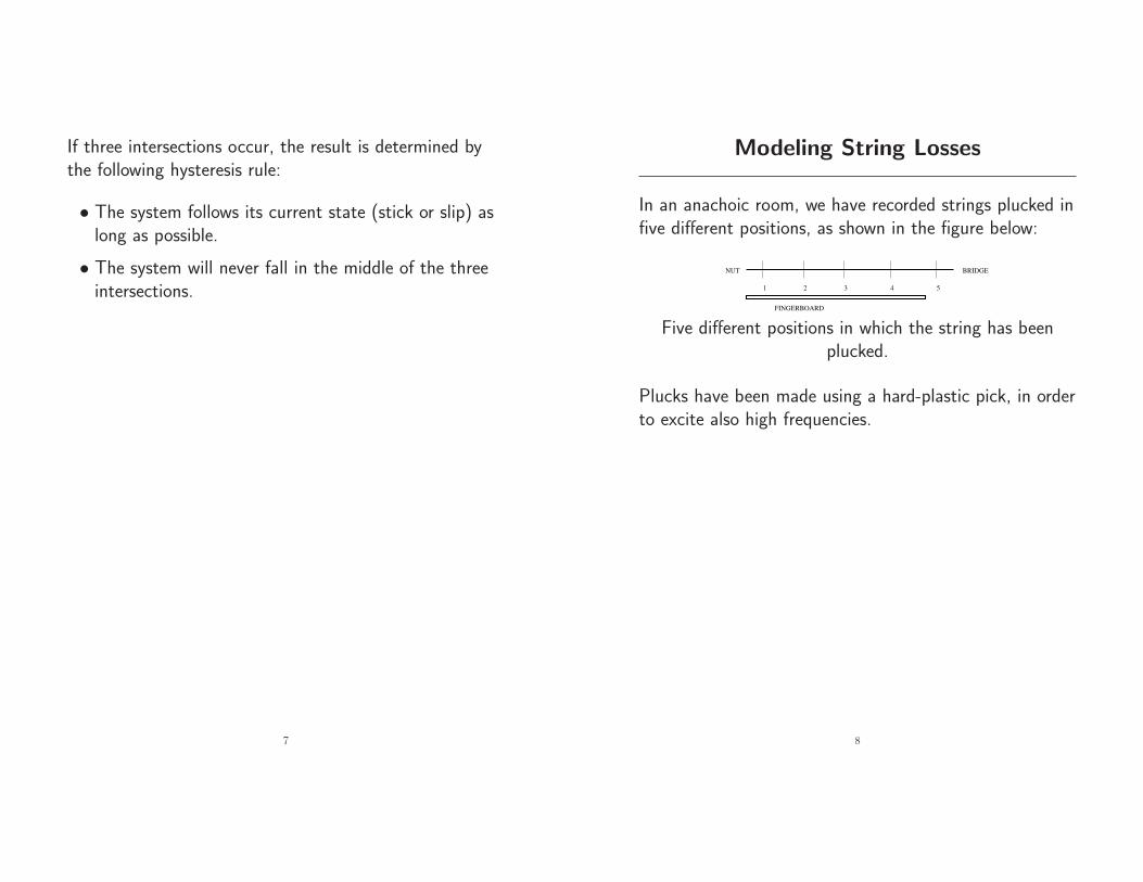
Modeling String Losses

In an anachoic room, we have recorded strings plucked infive different positions, as shown in the figure below:

1 2 3 54

BRIDGENUT

FINGERBOARD

Five different positions in which the string has beenplucked.

Plucks have been made using a hard-plastic pick, in orderto excite also high frequencies.

8

Analysis by Energy Decay Relief (EDR)

Violin G string

0

5

10

15

20

25 0

2

4

6

8

10−120

−100

−80

−60

−40

−20

0

20

40

Time (frames)

SOL1.wav − Energy Decay Relief

Frequency (kHz)

Magnitude (

dB

)

Plucked violin G string.

0

5

10

15

20

25 0

2

4

6

8

10−100

−80

−60

−40

−20

0

20

40

Time (frames)

sol1wf.wav − Energy Decay Relief

Frequency (kHz)

Magnitude (

dB

)

Plucked violin G string, with the nut side damped.

9

0

5

10

15

20

25 0

2

4

6

8

10−100

−80

−60

−40

−20

0

20

40

Time (frames)

la1.wav − Energy Decay Relief

Frequency (kHz)

Magnitude (

dB

)

Plucked violin A string.

0

5

10

15

20

25 0

2

4

6

8

10−120

−100

−80

−60

−40

−20

0

20

40

Time (frames)

la1wf.wav − Energy Decay Relief

Frequency (kHz)

Magnitude (

dB

)

Plucked violin A string, with the nut side damped.

10

Calculation of the decay rate of thepartials

• We calculate the slope of every partial in a db scale,to get the decay rate.

• The decay time is used to obtain the low-pass filtersthat estimate losses.

11

Accounting for Torsional Waves

Torsional waves can be modeled as an additional coupleof waveguides whose speed is about 5.2 times thetransverse wave speed.

vh = vin + vib + vint + vibt

von = vib +f

2Z

vob = vin +f

2Z

vont = vibt +f

2Zt

vobt = vint +f

2Zt

String String Bridge

BOW

vbpbvb

Control parameters

String Bridge

−1

−1String

(nut side,

trasversal waves)

(nut side,

torsional waves) trasversal waves)

(bridge side,

(bridge side,

torsional waves)

Structure of the basic model with filter in the nut sideand torsional waves.

12

where f = applied force

Z = string transverse wave impedance

Zt = string torsional wave impedance,

Torsional waves facilitate the establishment of Helmholtzmotion because they are more damped than thetransversal waves.Their contribution at the bow point can be modeled intwo ways:

1. Changing the slope of the straight line:

Zs =1

12Z + 1

2Zt

2. Changing the inclination of the friction curve

v-vb

f

13

Modeling the stiffness of the string

The stretching of the frequencies of the partials can becalculated as:

fn = nf0√1 +Bn2

where B = π3Ed4

64l2T=inharmonicity factor,

f0 =fundamental frequency of the string.

E=Young modulus of elasticity, d=diameter.

0 5 10 15 20 25 30 35 40 45 500

1000

2000

3000

4000

5000

6000

7000

8000

9000

10000

Shift of partials for a cello D string, f0=147 Hz,B=3e-4.x-axis: partial number, y-axis: frequency (Hz)

14

Physical constants of a Dominant violin string, fromPickering

String E (N/m) d(m) l (m) T B

E 15.7 0.000307 0.565 72.56 5.1627e-15A 7.470 0.000676 0.59 56.25 6.5418e-14D 6.4 0.000795 0.567 43.72 1.5707e-12G 6.035 0.000803 0.567 44.57 1.4963e-12

Physical constants of a gut violin string, from Schelleng.

String B

E 1.5598e-05A 4.8527e-05D 2.4841e-04G 1.3e-3

15

Designing allpass filters for dispersionsimulation

We choose a numerical filter made of a delay line delayline qτ−τ0, and a n-order stable all-pass filter:

H(q) = qnP (q−1)/P (q)

where

P (q) = p0 + . . . + pn−1qn−1 + qn

and τ and n are appropiately chosen.

We minimize the infinity-norm of a particular frequencyweighting of the error between the internal loop phaseand its approximation by the filter cascade:

δD = minp1,...,pm

‖WD(Ω)[ϕd(Ω)− (ϕD(Ω) + τΩ)]‖∞

where ϕD(Ω) =phase of H(ejΩ),WD(Ω) = frequency weigthing (WD(Ω) is zero outsidethe frequency range), i.e. [Ωc,ΩN ].

16

Results

The figure below shows the results given by thealgorithm, for a cello string (147 Hz) with B = 3e− 4.

0 1000 2000 3000 4000 5000 6000 7000 8000 9000 10000−10

−8

−6

−4

−2

0

2

4

6

8

10Erreur frequentielle finale sur les partiels

Frequency error (in cent) after the allpass filter approximation, for a cello D string..

17

0 1000 2000 3000 4000 5000 6000 7000 8000 9000 10000−10

−8

−6

−4

−2

0

2

4

6

8

10Erreur frequentielle finale sur les partiels

Frequency error (in cent) after the allpass filter approximation, for a violin A string, with

B = 4.8527e− 5.

String String Bridge

BOW

vbpbvb

Control parameters

String BridgeString

(nut side,

trasversal waves)

(nut side,

torsional waves) trasversal waves)

(bridge side,

(bridge side,

torsional waves)

Dispersion−1

−1

18

The friction models used in these simulations are:

• an hyperbola

µ = µd +(µs − µd)v0

v0 + v − vb

µd = 0.3 , µs = 0.8.

a sum of decaying exponentials:

µ = 0.4 ev−vb0.01 + 0.45 e

v−vb0.1 + 0.35

19

• a plastic model recently proposed by JimWoodhouse, who discovered that friction does notdepend only on the relative velocity between the bowand the string.

0.17 0.172 0.174 0.176 0.178-0.3

-0.25

-0.2

-0.15

-0.1

-0.05

0

0.05

0.1

Time0.12 0.13 0.14 0.15 0.16 0.17

2

2.2

2.4

2.6

2.8

3

3.2

3.4

3.6

3.8

4

Time

0.12 0.13 0.14 0.15 0.16 0.170.4

0.45

0.5

0.55

0.6

0.65

0.7

0.75

Time-0.4 -0.3 -0.2 -0.1 0 0.11

1.02

1.04

1.06

1.08

1.1

1.12

1.14

1.16

Velocity

20

µ =Aky(T )

Nsgn(v)

where

A = contact area between the bow and the string

N = normal load

ky(T ) = shear yield stress as a function of the bow-string contact

• In the plastic model the key state variable governingthe friction force is the temperature of the contactregion.

• The notion of coefficient of friction is kept, butinstead of depending on sliding speed it depends oncontact temperature.

• The contact temperature, in turn, depends on thesliding velocity (recent history).

21

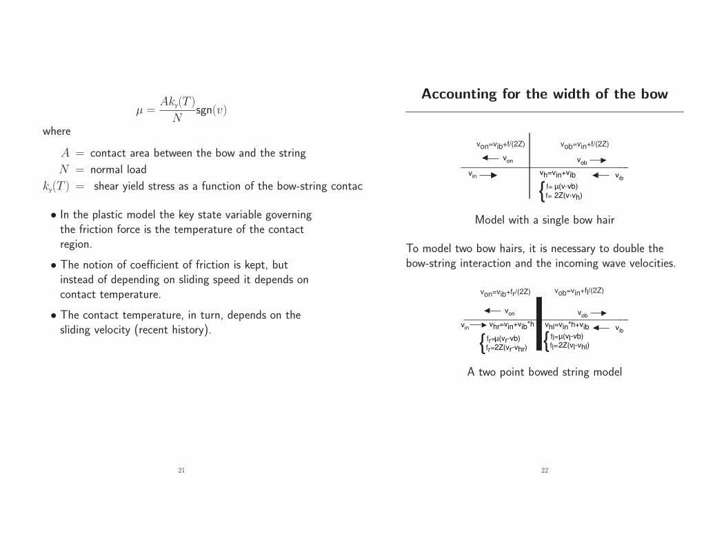
Accounting for the width of the bow

von vob

vibvin

vh=vin+vib

f= µ(v-vb)

2Z(v-vh)f=

vob=vin+f/(2Z)von=vib+f/(2Z)

Model with a single bow hair

To model two bow hairs, it is necessary to double thebow-string interaction and the incoming wave velocities.

von vob

vibvin

vhl=vin*h+vib

fl=µ(vl-vb)

2Z(vl-vhl)fl=

vob=vin+fl/(2Z)

fr=µ(vr-vb)

2Z(vr-vhr)fr=

von=vib+fr/(2Z)

vhr=vin+vib*h

A two point bowed string model

22

4000 4500 5000 5500 6000 6500 7000 7500 8000

−0.2

0

0.2A

mp

litu

de

4000 4500 5000 5500 6000 6500 7000 7500 8000

−0.2

0

0.2

4000 4500 5000 5500 6000 6500 7000 7500 8000

−0.2

0

0.2

4000 4500 5000 5500 6000 6500 7000 7500 8000−0.4

−0.2

0

0.2

Time (samples)

Simulation results from top to bottom: basic model,basic model with torsional waves, basic model with

torsional waves and string stiffness, model with torsionalwaves, string stiffness and bow width.

23

Calculation of the playability

What does playability mean?

“Playability” can be defined as the region of amultidimensional space given by the parameters of themodel where a good tone is obtained, where by goodtone, we usually mean the Helmholtz motion.

3

51

4

26

7

8

• The string sticks to the bow for most of the time,slipping backwards just once per vibration period.

24

• String motion:

Time

0

Str

ing v

eloci

ty

Time

Bri

dg

e fo

rce

Motion of a bowed string during an ideal Helmholtzmotion. String velocity at the bowed point and

trasverse force exerted by the string on the bridge.

25

Other kinds of motions

(pictures from the computer simulated model)

• Multiple slipsThe bow force is not high enough to allow the bow tostick throughout the nominal sticking period of theHelmholtz motion.

0 500 1000 1500 2000 2500 3000 3500-0.25

-0.2

-0.15

-0.1

-0.05

0

0.05

0.1

0.15

0.2

0.25

• Anomalous low frequencyA periodic note with a lower pitch can be producedwith a control of the bow force that makes thetransversal waves to miss a slip opportunity few timesin the stick-slip motion.

0 500 1000 1500 2000 2500 3000 3500-5

-4

-3

-2

-1

0

1

2

3

4

26

• Non-periodic motionsIrregular motion obtained when the bow force is toohigh.

0 500 1000 1500 2000 2500 3000 3500-1.5

-1

-0.5

0

0.5

1

1.5

27

Toward a Measure of Playability

The Schelleng diagram (1973)

Minimum bow force

Maximum bow force

Sul ponticello

Brilliant

Sul tasto

0.01 0.02 0.04 0.06 0.1

0.001

0.1

1

Relative position of bow, ß

Re

lative

fo

rce

RAUCOUS

NORMAL

0.2

0.01

HIGHER MODES

Inside the two straight line is the region where theHelmholtz motion is obtained.

28

Formulas for the Schelleng diagram

fmax =2Zvb

(µs − µd)β

fmin =Z2

2r1· vb

(µs − µd)β2

where µs=coefficient of static frictionµd=coefficient of dynamic frictionvb=bow velocityβ=bow positionZ=characteristic impedance of the string,Z =

√Tρ

r1=term that represents losses of the string

29

Simulation Parameters

• In the first simulations we examine a cello D string,with bending stiffness B = 0.0004 N m2.

• The string, starting from rest, is excited by a constantbow velocity vb = 0.05m/s.

• The Schelleng diagram is computed by varying thebow force fb from 0.005 to 5N , and the normalizeddistance β of the bow from the bridge is variedbetween 0.02 and 0.4 (where 0.5 would be the middleof the bow).

• A classifier routine examines the shape of theestablished waveforms.

In the second simulations we fix the bow position to 0.08,where 0 represents the bridge while 1 represents the nut,and we vary bow velocity and bow force.

30

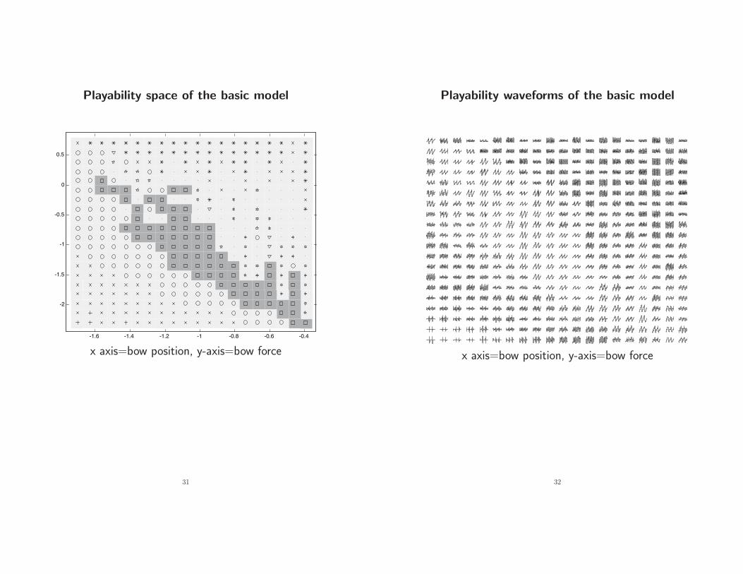
Playability space of the basic model

-1.6 -1.4 -1.2 -1 -0.8 -0.6 -0.4

-2

-1.5

-1

-0.5

0

0.5

x axis=bow position, y-axis=bow force

31

Playability waveforms of the basic model

x axis=bow position, y-axis=bow force

32

Velocity versus force playability space of thebasic model

-1.6 -1.4 -1.2 -1 -0.8 -0.6 -0.4

-2

-1.5

-1

-0.5

0

0.5

x-axis=bow velocity, y-axis=bow force

33

3D playability space of the basic model

−2

−1.5

−1

−0.5

0

−2

−1.5

−1

−0.5

0

0.5

1

0

0.2

0.4

0.6

0.8

1

log10(beta)log10(force)

(ve

locity)

34

-1.6 -1.4 -1.2 -1 -0.8 -0.6 -0.4

-2

-1.5

-1

-0.5

0

0.5

x-axis: bow position, y-axis:bow force

35

Velocity versus force playability space of thedamped model

-1.6 -1.4 -1.2 -1 -0.8 -0.6 -0.4

-2

-1.5

-1

-0.5

0

0.5

x-axis= bow velocity, y-axis= bow force

36

Playability space of the model with torsionalwaves

-1.6 -1.4 -1.2 -1 -0.8 -0.6 -0.4

-2

-1.5

-1

-0.5

0

0.5

x axis=bow position, y-axis=bow force

37

Waveforms playability space of the model withtorsional waves

x-axis=bow position, y-axis bow force

38

Velocity versus force playability space of themodel with torsional waves

-1.6 -1.4 -1.2 -1 -0.8 -0.6 -0.4

-2

-1.5

-1

-0.5

0

0.5

x-axis=bow velocity, y-axis=bow force

39

3D playability of the model with torsional waves

−2

−1.5

−1

−0.5

0

−1

−0.5

0

0.5

10

0.2

0.4

0.6

0.8

1

log10(beta)log10(force)

log

10

(ve

locity)

40

Velocity versus force playability of the modelwith stiffness

-1.6 -1.4 -1.2 -1 -0.8 -0.6 -0.4

-2

-1.5

-1

-0.5

0

0.5

Playability of the model with stiffness, x-axis=bowvelocity, y-axis=bow force

41

Playability of the model with stiffness

x-axis= bow position, y-axis= bow force

42

3D playability of the model with stiffness

−1.8−1.6

−1.4−1.2

−1−0.8

−0.6

−2

−1.5

−1

−0.5

0

0.5

1

0

0.1

0.2

0.3

0.4

0.5

0.6

0.7

0.8

0.9

log10(beta)log10(force)

log10(v

elo

city)

43

Conclusions

• Refined models of a bowed string are nowadayspossible.

• In this document we did not present a model for thebody of the instrument.

• The bow hair compliance can be further improved bycreating a finite-difference bow-width model.

44