Impact of whitecap coverage derived from a wave model on theassimilation of radiances from microwave imagers

Louis-François Meuniera, Stephen Englishb, and Peter Janssenb

aMétéo-France and CNRS,CNRM-GAME/GMAP, Toulouse, FrancebEuropean Centre for Medium-Range Weather Forecasts, Reading, United Kingdom

June 3, 2014

Abstract The assimilation of radiances from microwave imagers, relies on an accuraterepresentation of the surface properties in a radiative transfer model. The ECMWF IFS 4D-Var assimilation system uses the RTTOV radiative transfer model where microwave surfaceemissivity over oceans is computed by the FASTEMmodel. The ocean emissivity is influencedby the emissivity of the salted-water, the wave properties and also the whitecap coverage. Ithas been shown that, at large wind speeds, RTTOV exhibits an important bias for radiancesfrom microwave imagers that could be linked to a misrepresentation of the satellite pixelfraction covered by foam.The current FASTEM whitecap fraction depends only upon the 10m wind speed. Severalstudies have shown that it also depends on other parameters, such as the sea state. In theIFS, the atmospheric and wave models are coupled. Therefore, a comprehensive informationon the sea state is readily available to RTTOV. This capability has been used to implementa new whitecap fraction parametrisation depending upon observation time and location.Given the lack of global in situ observations of the whitecap fraction, the new parametrisationis evaluated within an assimilation experiment where the whitecap fraction estimate is usedby RTTOV. Positive results are noticed regarding the first-guess departure biases but thestandard deviations are slightly degraded. In order to understand these results, a retrieval ofwhitecap fraction has been set-up to act as a reference. The analysis of the results unveilsdeficiencies in other components of the FASTEM model and most likely in the foam emissivityparametrisation.Acknowledgement This study has been carried out within the context of the EUMETSATSatellite Application Facility on Numerical Weather Prediction (NWP SAF). The full reportof the Visiting Scientist mission (NWP_VS12_02) is availlable on the NWP SAF website(http://www.nwpsaf.eu/).

1 Introduction

In current data assimilation systems, satellite observations give the most important contribution tothe atmospheric analysis especially over data sparse area such as oceans. For each observation, amodel equivalent has to be calculated. Regarding satellite data, brightness temperatures have to becomputed from the data assimilation system a priori information using a radiative transfer model.

At ECMWF, in the IFS numerical weather prediction system, an incremental 4D-Var formulationis used (see [Courtier et al., 1994] and [Rabier et al., 2000]). The a priori information comes froma short range forecast started from the previous analysis. In order to assimilate satellite brightnesstemperatures, the observation equivalent is calculated using the RTTOV radiative transfer code

1/18

(see [Saunders et al., 1999]). At a given frequency in the microwave region, depending on thepolarization and viewing angle, the simulated brightness temperature can be expressed as follows:

TB = τrT↓ + τeTs + T↑, (1)

where TB is the simulated brightness temperature, τ is the atmospheric transmission from thesurface to space, e is the surface emissivity, r is the surface reflectivity (often assumed to be equalto 1 − e), T↓ is the atmospheric downward radiation (expressed as a brightness temperature), Ts isthe surface skin temperature and T↑ is the atmospheric upward radiation (expressed as a brightnesstemperature). τ , T↓, T↑ are computed from the model temperature and humidity profiles. Ts istaken from the background state and, over sea, e and r are calculated by the Fastem emissivitymodel (see [English and Hewison, 1998] and [Liu et al., 2011]).

Microwave imagers such as SSMI/S aboard DMSP satellites give a valuable information abouttemperature and moisture near the surface. At these frequencies the atmospheric absorption takesplace near the surface in a relatively thin layer of the atmosphere, hence the atmospheric transmis-sion to space τ is high. From Eq. (1) one can see that because of the high value of τ , a significantfraction of the brightness temperature measured by the satellite originates from the surface. Conse-quently, in order to obtain a useful information from these channels, it is crucial to have an accuratemodeling of the surface characteristics (e, r, and Ts).

Over sea, the Fastem model (currently version 5) is used to estimate the surface emissivity. Ittakes into account the emissivity of salted water but also the emissivity of the foam that may covera significant portion of the satellite footprint:

e = (1 −W )ewater +Wefoam, (2)

where W is the foam coverage, efoam is the foam emissivity and ewater is the foam-free sea wateremissivity.

• ewater is calculated from the Fresnel equation for a flat specular water surface (surface tem-perature and salinity being accounted for in the permittivity calculation). Then a two-scalecorrection is applied to take into account the effect of the surface roughness. The small scalecorrection, aims to parametrise the effect of small-scale ocean waves that are responsible forBragg scattering of the signal. The large scale correction is designed to account for reflec-tions due to large scale waves (as computed by a geometric optics model integrated overall wave slope facets). Apart from a viewing angle, polarization and frequency dependence,the two-scale correction is driven by the 10 meters wind speed1. The reader may refer to[Liu et al., 2011] for more details.

• efoam comes from an empirical parametrisation based on field measurements.

• W is parametrized using the 10 meter wind speed (see [Monahan and O’Muircheartaigh, 1986]).

At frequencies used by microwave imagers, the foam-free water emissivity is relatively low (es-pecially for the horizontally polarized channels) while the foam emissivity is close to one (on bothvertically and horizontally polarized channels). Consequently, even with a small amount of foamthe contribution on the total emissivity and to the simulated brightness temperature is large.

An attempt to improve the whitecap fraction parametrisation have been made in Fastem-4(see [Liu et al., 2011]). Nonetheless, Fastem-5 reverted back to the previous formulation (cited

1The large scale correction is not only depending on the wind speed but also on the stage of development of thelarge scale waves, e.g. on the wave age. This is ignored in Fastem.

2/18

above). [Bormann et al., 2012] show that with any of these parametrisations a significant biasremains in high wind speed areas, especially for microwave imagers. Therefore, whitecap fractionparametrisation needs to be further addressed in order to improve the skills of microwave oceansurface emissivity models at high wind speed.

In this document, we examine the impact of a new foam coverage parametrisation on simulatedbrightness temperatures and evaluate its effect on the accuracy of the atmospheric analyses. Inthe first part we focus on the foam coverage parametrisation itself and highlight the differencesbetween the current Fastem-5 parametrisation and the proposed formulation. In the second part,we discuss the impact of the new parametrisation on simulated brightness temperatures. The lastpart shows some promising results of a first attempt to retrieve the whitecap fraction from satellitemeasurements.

2 Whitecap fraction parametrisation

2.1 Whitecap fraction calculation from wave model fields

[Anguelova and Webster, 2006] made an extensive survey of wind speed driven foam fraction parametri-sations. All are obtained by fitting a wind speed function to an observational dataset. These variousparametrisations exhibit a very large spread in modelled whitecap coverage (variations of severalorders of magnitude for a given wind speed). Several hypotheses are given to explain such largediscrepancies :

• Whitecap fraction parametrisations based on wind speed alone do not account for manyfactors affecting the whitecap coverage: sea state (swell, significant wave height, wave age,...), surface currents, atmospheric stability near the surface, salinity, sea surface temperature,surface surfactant concentration...

• Observational datasets used to establish the wind speed based parametrisations can be ob-tained in very different conditions (warm or cold seas, open ocean or fetch limited areas, ...).This can partly explains the large differences between the various formulations. Moreoverthese datasets do not cover the whole globe: most of them were obtained in coastal areas andfew observations are available in the southern hemisphere;

• The whitecap fraction measurement itself (usually based on photographic analysis) can alsolead to uncertainties.

Other parametrisations have been developed in order to better take into account the sea state(see [Goddijn-Murphy et al., 2011] for a review of these parametrisations). In this study we examinea new parametrisation based on wave model outputs. Such models give a detailed description ofthe full wave spectrum which in turns can be used to provide information on the sea state. Wavemodels such as the WAMmodel coupled to IFS (see [Janssen et al., 2005]) are based on the followingequation:

DF (ω, θ)

Dt= Sin(ω, θ) + Snl(ω, θ) + Sds(ω, θ), (3)

where F is the wave variance spectrum (that depends on the frequency, ω, and direction, θ), Sin isthe source term for wind input, Snl is for the nonlinear interactions and Sds is the energy dissipation.Bottom friction set aside, it is assumed that wave breaking is the dominant mechanism for energy

3/18

dissipation and that each breaking event produces whitecaps. The energy flux from waves to oceanis given by:

Φoc = ρwg

∫Sdsdθdω. (4)

Following [Kraan et al., 1996], it is possible to calculate the whitecap fraction from the modelledenergy flux from waves to ocean:

Φoc = −γρwgWωpE, (5)

where, E is the total wave variance, ωp is the angular peak frequency, W is the whitecap fraction,γ is the average fraction of the total wave energy dissipated per whitecapping event. Melville andRapp (1985) suggested a value of γ = 0.005. This constant value has been chosen in our firstattempt to calculate the whitecap fraction.

From eq. (4) and (5), W can be written as:

W = − Φoc

γρwgEωp, (6)

where Φoc, E and ωp are calculated by the wave model.

It should be noted that:

• Since the peak angular frequency may jump from one mode to another when wind sea andswells are combined, in practice, ωp is assumed to be equal to the mean angular frequency ofthe wind-sea.

• E is linked to the significant wave height HS by E = HS2/16.

W can also be expressed as a combination of normalized variables:

W = −εmχγE∗

, (7)

where ε = ρa/ρw, E∗ is the dimensionless wave variance E∗ = g2E/u4∗ (u∗ being the frictionvelocity), m is the normalised dissipation m = −Φoc/ (ρau

3∗) and χ is the wave age χ = g/(ωpu∗).

In this whitecap fraction parametrisation, the dependence on the sea state is driven by Φoc,E and ωp. There is no direct dependence on the wind speed, but the modeled Φoc is influencedby it. Restriction to the case of pure wind sea, one can demonstrate that this parametrisation isconsistent with the one introduced in [Kraan et al., 1996] where W is roughly proportional to χ−2.Small values of χ indicate young wind-seas whereas large values of χ indicate well developed seas.Consequently, the parametrisation ofW defined in Eq. (6) gives higher whitecap fractions for youngwind-seas.

This parametrisation based on wave energy dissipation should be able to better represent thewhitecap fraction variability compared to the Fastem-5 parametrisation that is solely based on the10m wind speed. Nonetheless, parameters like atmospheric stability, salinity, sea surface tempera-ture or surface currents are not taken into account which can lead to noticeable differences betweendiagnosed and observed whitecap fraction. Even though a few parameters are neglected, becauseit is linked to the amount of dissipated energy, the new parametrisation should have good skill atpredicting the amount of newly generated whitecap (often referred as Stage A foam). On the otherhand, the amount of decaying foam (Stage B foam) will be less accurately predicted since the foamdecay time greatly vary with parameters such as the surface surfactant concentration or the seasurface temperature (see [Callaghan et al., 2012]).

4/18

2.2 Whitecap fraction calculation from IFS/WAM fields

All the necessary input fields are readily available from the ECMWF operational archive. Usingshort terms forecasts, we have calculated whitecap fraction fields every 6 hours over a 2 monthsand a half period from 1st October 2012 to 14th December 2012. Mean whitecap fraction fields arepresented in Figure 1 using the mean frequency of the wind-sea (a).

0°

20°N

40°N

60°N

0°

20°S

40°S

60°S

0° 60°E 120°E180° 180°120°W 60°W 0°0°60°W120°W180° 180°

ECWAM: 01/10/12 12h to 14/12/12 18h - Mean

0.0

0.4

0.8

1.2

1.6

2.0

2.4

Whit

eca

p f

. (w

ith fws)

(%

)

(a) Using the mean frequency of the wind sea

0°

20°N

40°N

60°N

0°

20°S

40°S

60°S

0° 60°E 120°E180° 180°120°W 60°W 0°0°60°W120°W180° 180°

ECWAM: 01/10/12 12h to 14/12/12 18h - Mean

0.0

0.4

0.8

1.2

1.6

2.0

2.4

Whit

eca

p f

. M

M8

6 (

%)

(b) Using the 10m wind speed ([Monahan and O’Muircheartaigh, 1986])

Figure 1: Mean whitecap fraction cubic root field between 1st October 2012 and 14th December 2012, based onshort term forecasts of IFS/WAM, computed from various formulations.

Overall, the geographical distribution of the whitecap fraction diagnosed using the WAM model(Fig. 1.a) is close to the one given by the formula based on the wind speed (Fig. 1.b). Near thecoasts (Alaska), in sheltered area (Caribbean sea, North Sea, Mediterranean sea, Japan Sea) andin some regions where the ocean is relatively shallow (South of Argentina, North of the China sea),whitecap amounts diagnosed using the WAM model are higher. In those regions, because of thesmall fetch distance and of finite depth, the wave model produces steeper waves which in turnsdissipate more energy.

The wave model based parametrisation, shows a saturation of the whitecap fraction at high windspeeds (see Figure 2). This is in good agreement with the findings of [Goddijn-Murphy et al., 2011]who noticed evidences of such a saturation in field experiment measurements.

2.3 Conclusion

Because of the lack of global measurements of the whitecap fraction, it is difficult at this pointto determine which whitecap parametrisation and wave model performs best. The effect of thenew whitecap fraction parametrisation on the simulated brightness temperatures can be seen as anindirect validation.

5/18

0.0

0.5

1.0

1.5

2.0

2.5

[Whit

eca

p f

ract

ion (

%)]

1/3

Monahan and O'Muircheartaigh (1986)

Goddjin-Murphy (2011)

From wave model (using fws)

0 2 4 6 8 10 12 14 16 18 20 22 2410m windspeed (m/s)

0e+001e+062e+063e+064e+065e+066e+06

ECMWF: 01/10/12 12h to 14/12/12 18h

Figure 2: Mean whitecap fraction cubic root, with respect to wind speed, between 1st October 2012 and 14thDecember 2012. Based on short term forecasts of IFS/WAM. Error bars show the standard deviation.

The IFS code has been modified to allow the online calculation of the whitecap fraction fromthe wave model fields. Since the atmospheric model and wave model are fully coupled in the IFS,the diagnosed whitecap fraction is available at each model time-step. It can consequently be usedby Fastem during the surface emissivity calculation in an assimilation experiment.

3 Impact on the simulated brightness temperatures in IFS

3.1 Experiments setup

A version of IFS based on cycle 38r2 e-suite has been used. It also includes improved scatteringcoefficients for the microwave radiative transfer (see [Geer, 2013]). Compared to operations, theatmospheric model has been run at a lower truncation (T511L91) and in the incremental 4D-varalgorithm three outer loops have been performed at respectively T95, T159 and T255.

All the observations currently assimilated at ECMWF are used. Regarding satellite data, in-frared and microwave sounders are assimilated in clear sky conditions only, whereas microwave im-agers are also used in thick and precipitating clouds (see [Bauer et al., 2010] and [Geer et al., 2010]).For satellite and aircraft data, the variational bias correction (VarBC) is used (see [Dee, 2005]). Weuse the same predictors as in the operational IFS, but we have turned on the passive monitoring onall TRMM/TMI, Coriolis/Windsat and DMSP-F18/SSMIS channels.

Over the period of 1 October 2012 00UTC to the 14 December 2012 12UTC, two experimentshave been run:

6/18

• fwas (also referred as control): a baseline using the current wind-based whitecap fractionparametrisation of Fastem-5.

• fw76 (also referred as new): a experiment using the whitecap fraction parametrisation intro-duced in the previous section, based on the mean frequency of wind sea.

Because of the addition of new monitored channels and of the change for the emissivity cal-culation in the new experiment, the VarBC coefficients needs a few assimilation cycles to adjust.Based on an examination of the VarBC coefficients time-series (not shown) we discarded the firstnine days. The comparison between the two experiments will therefore start from the 10 October2012 00UTC.

3.2 Overall results

When dealing with data going through the Allsky route, one can define three cloudiness categoriessummarized in Table 1. For non-cloudy observations, the measured brightness temperature is verysensitive to the surface emissivity. For rainy observations, the atmosphere is nearly opaque. Ideally,in order to evaluate the whitecap fraction impact, one would like to use only non-cloudy observation.However, this sample exhibit a bias toward low wind speed values where the whitecap amount isknown to be small. Because of this trade-off between surface sensitivity and 10m wind speedsampling, we have chosen to focus on all the non-rainy observations.

LWP threshold SI threshold Approx. % of the totalNon-cloudy < 0.5kg/m2 < 40K 40%Non-rainy < 40K 90%Active 100%

Table 1: Cloudiness categories for Allsky observations. (LWP stands for the Liquid Water Path calculated from the22Ghz V and 37Ghz V channels. SI stands for the scattering index defined as the brightness temperature differencebetween the 37Ghz V and 37Ghz H channels.)

Results for the TMI imager are shown in Figure 3. At all wind speeds, the mean bias correctedfirst-guess departure is nearly unchanged. However, for low frequencies at high wind speeds the first-guess departures standard deviation are degraded when the new whitecap fraction parametrisationis used. This is not the case for the high frequency channels (around 90GHz) that are less sensitiveto the surface.

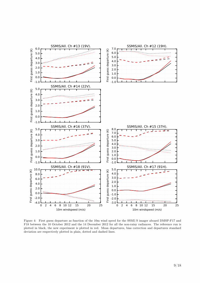
Results for the SSMI/S imaging channels aboard DMSP F17 and F18 are shown in Figure 4.SSMI/S has a global coverage whereas TMI only covers the area between 40°S and 40°N. SSMI/Sextended coverage allows to sample more high wind speed scenes so that the statistics for the 20-25m/s wind speed bin are shown in the plots of Figure 4. Statistics for SSMI/S and TMI arequite similar. The statistics for the highest wind speeds confirms that the new whitecap fractionparametrisation gives slightly degraded results especially for the low frequency channels that arealso the more sensitive to the surface emission.

For both TMI and SSMI/S, the plots show that overall, at low frequencies, the bias correctionbecomes less dependent on the 10m wind speed. This is backed up by the fact that VarBC coefficientsfor the 10m wind speed predictor are smaller in the experiment using the new whitecap fractionparametrisation.

7/18

0 2 4 6 8 10 12 15 20 2510m windspeed (m/s)

-2.0

0.0

2.0

4.0

6.0

8.0

10.0

Firs

t gue

ss d

epar

ture

(K)

TMI/TRMM. Ch #9 (86H).

0 2 4 6 8 10 12 15 20 2510m windspeed (m/s)

-0.5 0.0 0.5 1.0 1.5 2.0 2.5 3.0 3.5 4.0

Firs

t gue

ss d

epar

ture

(K)

TMI/TRMM. Ch #8 (86V).-4.0-2.0 0.0 2.0 4.0 6.0 8.010.0

Firs

t gue

ss d

epar

ture

(K)

TMI/TRMM. Ch #7 (37H).

-2.0-1.0 0.0 1.0 2.0 3.0 4.0 5.0

Firs

t gue

ss d

epar

ture

(K)

TMI/TRMM. Ch #6 (37V).-0.5 0.0 0.5 1.0 1.5 2.0 2.5 3.0 3.5

Firs

t gue

ss d

epar

ture

(K)

TMI/TRMM. Ch #5 (21V).-1.0 0.0 1.0 2.0 3.0 4.0 5.0 6.0

Firs

t gue

ss d

epar

ture

(K)

TMI/TRMM. Ch #4 (19H).

-0.5 0.0 0.5 1.0 1.5 2.0 2.5 3.0 3.5

Firs

t gue

ss d

epar

ture

(K)

TMI/TRMM. Ch #3 (19V).-2.0

-1.0

0.0

1.0

2.0

3.0

4.0

Firs

t gue

ss d

epar

ture

(K)

TMI/TRMM. Ch #2 (11H).

-2.0

-1.0

0.0

1.0

2.0

3.0Fi

rst g

uess

dep

artu

re (K

)TMI/TRMM. Ch #1 (11V).

Figure 3: First guess departure as function of the 10m wind speed for the TRMM/TMI imager between the 10October 2012 and the 14 December 2012 for all the non-rainy radiances. The reference run is plotted in black, thenew experiment is plotted in red. Mean departures, bias correction and departures standard deviation are respectivelyplotted in plain, dotted and dashed lines.

8/18

0 2 4 6 8 10 12 15 20 2510m windspeed (m/s)

-4.0-2.0 0.0 2.0 4.0 6.0 8.010.0

Firs

t gue

ss d

epar

ture

(K)

SSMIS/All. Ch #18 (91V).

0 2 4 6 8 10 12 15 20 2510m windspeed (m/s)

-3.0-2.0-1.0 0.0 1.0 2.0 3.0 4.0 5.0

Firs

t gue

ss d

epar

ture

(K)

SSMIS/All. Ch #17 (91H).-1.0

0.0

1.0

2.0

3.0

4.0

5.0

Firs

t gue

ss d

epar

ture

(K)

SSMIS/All. Ch #16 (37V).

-1.0 0.0 1.0 2.0 3.0 4.0 5.0 6.0 7.0 8.0

Firs

t gue

ss d

epar

ture

(K)

SSMIS/All. Ch #15 (37H).-1.0

0.0

1.0

2.0

3.0

4.0

5.0

Firs

t gue

ss d

epar

ture

(K)

SSMIS/All. Ch #14 (22V).-1.0 0.0 1.0 2.0 3.0 4.0 5.0 6.0

Firs

t gue

ss d

epar

ture

(K)

SSMIS/All. Ch #13 (19V).

-1.0 0.0 1.0 2.0 3.0 4.0 5.0 6.0 7.0

Firs

t gue

ss d

epar

ture

(K)

SSMIS/All. Ch #12 (19H).

Figure 4: First guess departure as function of the 10m wind speed for the SSMI/S imager aboard DMSP-F17 andF18 between the 10 October 2012 and the 14 December 2012 for all the non-rainy radiances. The reference run isplotted in black, the new experiment is plotted in red. Mean departures, bias correction and departures standarddeviation are respectively plotted in plain, dotted and dashed lines.

9/18

3.3 Geographical distribution

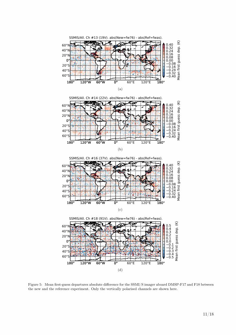
Statistics for TMI and SSMI/S have been aggregated on a 2.5°x2.5° lat/lon grid during the trialperiod (from 10 October 2012 to 14 December 2012). For the SSMI/S imaging channels (verticalpolarisation only), Figure 5 shows the difference of the absolute values of the bias corrected first-guess departure between the new and the reference experiment. At frequencies between 19 and37GHz, for both polarisations, the mean first guess departure is increasing in several coastal areasand/or sheltered seas (Caribbean Sea, Tip of Argentina, China sea, Mediterranean sea).

Over the North Atlantic ocean and the South Indian ocean, the standard deviation of the first-guess departures tends to increase when the new whitecap fraction parametrisation is used (mapsnot shown). This is in good agreement with Figure 4 since high wind speed values are usuallyobserved in those regions

Statistics from TMI (maps not shown) lead to similar conclusions.

3.4 Summary

The use of a whitecap fraction diagnosed from the wave model outputs, gives us promising resultsregarding the bias of the radiative transfer simulations with respect to the wind speed. However,the whitecap fraction parametrisation still needs to be improved. The degradation of the first-guessdepartures standard deviation at high wind speed, might be reduced by a better tuning of theparametrisation.

The increase of the first-guess departures biases in coastal and sheltered areas is probably linkedto an excess of whitecap. In section 2.2, this has been explained by the fact that, in such areas,waves are steeper which leads to a higher amount of dissipated energy. Since, the γ parameterin Eq. 5 has been set to a constant value in our experiment, this translates directly into higheramounts of whitecap. Therefore, a way to tune the whitecap fraction parametrisation would be toconsider γ as a function of the wave steepness or more generally of the sea state.

4 Whitecap fraction retrieval

4.1 Retrieval method and experiment setup

Whitecap fraction retrievals from microwave imager measurements have already been successfullyused to derive statistics on the global whitecap coverage (see [Anguelova and Webster, 2006]). InFastem-5, the emissivity is calculated as follows:

e = (1 −W )ewater +Wefoam, (8)

where, ewater and efoam are either calculated or empirically parametrised in Fastem. [Prigent et al., 2005]and [Karbou et al., 2006] have demonstrated that it was possible to retrieve the total emissivity fromsatellite measurements. Therefore, given our knowledge of ewater and efoam it is possible to retrievethe whitecap fraction W .

The IFS experiment used for the whitecap retrieval (fwl6) is configured in a similar manner tothe new experiment (fw76) described in section 3.1. However, in the VarBC setup, the use of the10m wind speed predictor has been removed. Using the 10m wind speed predictor would lead tounrealistic whitecap fraction estimates since the observed brightness temperature used during theemissivity retrieval would be bias corrected for the whitecap fraction parametrisation deficiencies.

10/18

0°

20°N

40°N

60°N

0°

20°S

40°S

60°S

0° 60°E 120°E180° 180°120°W 60°W 0°0°60°W120°W180° 180°

SSMIS/All. Ch #13 (19V). abs(New=fw76) - abs(Ref=fwas).

0.400.320.240.160.08

0.000.080.160.240.320.40

Mean f

irst

guess

dep.

(K)

(a)

0°

20°N

40°N

60°N

0°

20°S

40°S

60°S

0° 60°E 120°E180° 180°120°W 60°W 0°0°60°W120°W180° 180°

SSMIS/All. Ch #14 (22V). abs(New=fw76) - abs(Ref=fwas).

0.400.320.240.160.08

0.000.080.160.240.320.40

Mean f

irst

guess

dep.

(K)

(b)

0°

20°N

40°N

60°N

0°

20°S

40°S

60°S

0° 60°E 120°E180° 180°120°W 60°W 0°0°60°W120°W180° 180°

SSMIS/All. Ch #16 (37V). abs(New=fw76) - abs(Ref=fwas).

0.400.320.240.160.08

0.000.080.160.240.320.40

Mean f

irst

guess

dep. (K

)

(c)

0°

20°N

40°N

60°N

0°

20°S

40°S

60°S

0° 60°E 120°E180° 180°120°W 60°W 0°0°60°W120°W180° 180°

SSMIS/All. Ch #18 (91V). abs(New=fw76) - abs(Ref=fwas).

0.50.40.30.20.1

0.00.10.20.30.40.5

Mean f

irst

guess

dep.

(K)

(d)

Figure 5: Mean first-guess departures absolute difference for the SSMI/S imager aboard DMSP-F17 and F18 betweenthe new and the reference experiment. Only the vertically polarised channels are shown here.

11/18

The accuracy of the emissivity retrieval strongly depends on the accuracy of the IFS first guessand of the RTTOV simulation. To avoid cases where the atmosphere is nearly opaque, we willconsider only the non-rainy radiances (see Table 1) with a more stringent threshold on the scatteringindex (50K instead of 40K).

4.2 Validity of the results

For each sensor and frequency, the retrieved whitecap fraction can be averaged on a 2.5°x2.5°lat/lon grid for the experiment duration (between the 10 October 2012 and the 14 October 2012).Independently, we apply the same sampling to the whitecap fraction diagnosed from the wave model.

At low frequencies (10 to 22GHz), the geographical distribution of the mean retrieved whitecapfraction is in good agreement with the diagnosed whitecap fraction (see Figure 6). In this rangeof frequency, results are consistent across sensor types (TMI, SSMI/S and WindSat) and polarisa-tions. In section 3.3, when the new whitecap fraction parametrisation is used, we have noticed adegradation of the first-guess departures in some coastal and sheltered areas. That was linked toan increase in the whitecap amount compared to the wind-based formula. The whitecap fractionretrieval shows no evidence of such an increase in the whitecap amount which confirm the need ofre-tuning of the new whitecap fraction parametrisation.

At higher frequencies (37 and 90GHz), the whitecap retrievals are dominated by biases in theradiative transfer and model (not shown). At 37GHz, marine stratocumulus in the trade wind areasseem to be the main cause of bias. At 90GHz, excessive amount of whitecap are also diagnosed underthe thicker clouds around the ITCZ and PTCZ. Consequently, we will not use whitecap retrievalsat such high frequencies.

0°

20°N

40°N

60°N

0°

20°S

40°S

60°S

0° 60°E 120°E180° 180°120°W 60°W 0°0°60°W120°W180° 180°

SSMIS/All. Ch #13 (19V). Expver=fwl6.

0.00.30.60.91.21.51.82.12.4

Retr

ieved w

hit

eca

p f

.(%

)

(a) Retrieved whitecap fraction

0°

20°N

40°N

60°N

0°

20°S

40°S

60°S

0° 60°E 120°E180° 180°120°W 60°W 0°0°60°W120°W180° 180°

SSMIS/All. Ch #13 (19V). Expver=fwl6.

0.00.30.60.91.21.51.82.12.4

Dia

gnose

d w

hit

eca

p f

. (%

)

(b) Diagnosed whitecap fraction (from the wave model)

Figure 6: Mean retrieved and diagnosed whitecap fraction for SSMI/S channel 2 (19 GHz V) aboard DMSP F17and F18

12/18

Statistics with respect to the 10m wind speed (see Figure 7) show that uncorrected biases remainin the atmospheric model or radiative transfer code. Indeed, especially at low wind speeds, negativemean whitecap fractions are obtained: since in the retrieval experiment there is no VarBC predictorbased on the 10m wind speed, VarBC ensures that the bias is corrected when all wind speeds areconsidered but this does not guarantee that the bias is null for a given wind speed (notably at0m/s). This causes the offset on the whitecap fraction retrieval curves but does not affect theshape of the curves.

0 2 4 6 8 10 12 15 20 2510m windspeed (m/s)

2

0

2

4

6

8

Whit

eca

p f

ract

ion (

%)

WAM

19V

22V

37V

91V

0 2 4 6 8 10 12 15 20 2510m windspeed (m/s)

2

0

2

4

6

8WAM

19H

37H

91H

SSMIS/All. Expver=fwl6.

(a) SSMI/S aboard DMSP F17 and F18

0 2 4 6 8 10 12 15 20 2510m windspeed (m/s)

2

0

2

4

6

8

Whit

eca

p f

ract

ion (

%)

WAM

11V

19V

21V

37V

86V

0 2 4 6 8 10 12 15 20 2510m windspeed (m/s)

2

0

2

4

6

8WAM

11H

19H

37H

86H

TMI/TRMM. Expver=fwl6.

(b) TMI aboard TRMM

Figure 7: Retrieved whitecap fraction for the SSMI/S and TMI sensors with respect to the wind speed.

Figure 7 shows that the retrieved whitecap fraction varies with frequency and polarisation. Ata given frequency and for high incidence angle (around 53° for SSMI/S and TMI), the emissivityof the foam is significantly smaller for the horizontal polarisation than for the vertical one. Sucha difference between the two polarisations is taken into account in the Fastem foam emissivityparametrisation, however the comparison to laboratory measurements (see [Rose et al., 2002]) sug-gests that the emissivity for the horizontal polarisation might be overestimated in Fastem whichwould explain the lower amount of retrieved whitecap for the horizontal polarisations.

13/18

For a given polarisation, the retrieved whitecap fraction decreases with increasing frequencies.This could arise from an improper parametrisation of the foam emissivity in Fastem where theemissivity increases with the frequency. Indeed, [Rose et al., 2002] laboratory measurements at10.8 and 36.5GHz show no evidence of such an increase.

In this study, we have exclusively studied mean values of the retrieved whitecap fraction (forspecific wind speeds and locations). In theory, the retrieved whitecap fraction could give us anindication about the statistical distribution of the whitecap fraction for a given wind speed. Thiswould help to evaluate the ability of the wave model based parameterisation to take into accountthe sea state (that is currently ignored in Fastem). However, prior to such an evaluation, the errorof the whitecap fraction retrieval itself should be carefully examined. Indeed, the spread of theretrieved whitecap fraction is greatly influenced by the quality of the background fields used for theretrieval or by the quality of the other components of the radiative transfer model.

4.3 Summary

Emissivity retrievals are a valuable tool to evaluate the biases of whitecap parametrisations over agiven area. Moreover, the comparison between retrieved whitecap amounts at various frequenciesand polarisations gives an insight on the performances of the emissivity models for the foam andthe foam-free water.

Retrievals at low frequencies confirm results of section 3.3 in coastal and sheltered areas. More-over, overall statistics stress out the need of additional work on the emissivity model of the foam.The current parametrisation of the foam emissivity is based on Stogryn empirical model and hasbeen modified in Fastem-4. However, compared to laboratory measurements, differences remainand need to be addressed. This work on the foam emissivity would benefit to all whitecap parametri-sations.

5 Conclusion and perspectives

In the present study, a whitecap fraction parametrisation based on wave model outputs have beenapplied to the ECMWF wave model (WAM). This new parametrisation gives realistic results. How-ever the lack of in situ observations makes a direct evaluation of this parametrisation very difficult.

As an indirect validation, we have implemented this new whitecap fraction parametrisation ina development branch of the IFS model which allows us to run assimilation experiments using thenew whitecap fraction estimate in the RTTOV radiative transfer code. In terms of total bias, resultsare improved. However the standard deviation of the first guess departures are slightly degradedat high wind speeds for surface sensitive channels. Moreover, the new parametrisation seems togenerate excessive whitecap amounts in several coastal and sheltered areas.

In order to understand the new whitecap fraction parametrisation weaknesses and because of thelack of in situ observations, a whitecap fraction retrieval was attempted. It gives promising resultsfor low frequency imaging channels and allows us to confirm the new parametrisation deficiencies incoastal and sheltered areas. Unexpectedly, it also pointed out the need of a revised foam emissivityparametrisation within Fastem.

Recent laboratory measurements of the foam emissivity may be used to update the current empir-ical foam emissivity parametrisation. However, in the literature, measurements are usually availableonly at low frequencies. A more innovative approach would be to use physically-based foam emissiv-ity models such as the one developed at NRL (see [Anguelova, 2008] and [Anguelova et al., 2009]).

14/18

Physically-based models might be computationally too expensive to be integrated in Fastem butcould be used to derived a new regression-based parametrisation.

15/18

16/18

References

[Anguelova et al., 2009] Anguelova, M., Gaiser, P., and Raizer, V. (2009). Foam emissivity modelsfor microwave observations of oceans from space. In Geoscience and Remote Sensing Sympo-sium,2009 IEEE International,IGARSS 2009, volume 2, pages II–274–II–277.

[Anguelova, 2008] Anguelova, M. D. (2008). Complex dielectric constant of sea foam at microwavefrequencies. Journal of Geophysical Research: Oceans, 113(C8):n/a–n/a.

[Anguelova and Webster, 2006] Anguelova, M. D. and Webster, F. (2006). Whitecap coverage fromsatellite measurements: A first step toward modeling the variability of oceanic whitecaps. Journalof Geophysical Research: Oceans, 111(C3).

[Bauer et al., 2010] Bauer, P., Geer, A. J., Lopez, P., and Salmond, D. (2010). Direct 4d-var assim-ilation of all-sky radiances. part i: Implementation. Quarterly Journal of the Royal MeteorologicalSociety, 136(652):1868–1885.

[Bormann et al., 2012] Bormann, N., Geer, A., and English, S. (2012). Evaluation of the microwami-crowave ocean surface emissivity model FASTEM-5 in the IFS. Technical Report Memorandum667, Research Department, ECMWF, Reading, U. K.

[Callaghan et al., 2012] Callaghan, A. H., Deane, G. B., Stokes, M. D., and Ward, B. (2012).Observed variation in the decay time of oceanic whitecap foam. Journal of Geophysical Research:Oceans, 117(C9).

[Courtier et al., 1994] Courtier, P., Thépaut, J.-N., and Hollingsworth, A. (1994). A strategy foroperational implementation of 4d-var, using an incremental approach. Quarterly Journal of theRoyal Meteorological Society, 120(519):1367–1387.

[Dee, 2005] Dee, D. P. (2005). Bias and data assimilation. Quart. J. Roy. Meteor. Soc.,131(613):3323–3343.

[English and Hewison, 1998] English, S. J. and Hewison, T. J. (1998). Fast generic millimeter-waveemissivity model. Proc. SPIE, Microwave Remote Sensing of the Atmosphere and Environment,3508:288–300.

[Geer, 2013] Geer, A. J. (2013). All-sky assimilation: better snow-scattering radiative transfer andaddition of ssmis humidity sounding channels. Technical Report 706, ECMWF.

[Geer et al., 2010] Geer, A. J., Bauer, P., and Lopez, P. (2010). Direct 4d-var assimilation ofall-sky radiances. part ii: Assessment. Quarterly Journal of the Royal Meteorological Society,136(652):1886–1905.

[Goddijn-Murphy et al., 2011] Goddijn-Murphy, L., Woolf, D. K., and Callaghan, A. H. (2011).Parameterizations and algorithms for oceanic whitecap coverage. J. Phys. Oceanogr., 41(4):742–756.

[Janssen et al., 2005] Janssen, P., Bidlot, J.-R., Abdalla, S., and Hersbach, H. (2005). Progress inocean wave forecasting at ECMWF. Technical Report Memorandum 478, Research Department,ECMWF, Reading, U. K.

[Karbou et al., 2006] Karbou, F., Gérard, E., and Rabier, F. (2006). Microwave land emissivityand skin temperature for amsu-a and -b assimilation over land. Quarterly Journal of the RoyalMeteorological Society, 132(620):2333–2355.

17/18

[Kraan et al., 1996] Kraan, C., Oost, W., and Janssen, P. (1996). Wave energy dissipation bywhitecaps. Journal of Atmospheric and Oceanic Technology, 13(1):262–271.

[Liu et al., 2011] Liu, Q., Weng, F., and English, S. (2011). An improved fast microwave wateremissivity model. Geoscience and Remote Sensing, IEEE Transactions on, 49(4):1238–1250.

[Monahan and O’Muircheartaigh, 1986] Monahan, E. C. and O’Muircheartaigh, I. G. (1986).Whitecaps and the passive remote sensing of the ocean surface. International Journal of Re-mote Sensing, 7(5):627–642.

[Prigent et al., 2005] Prigent, C., Chevallier, F., Karbou, F., Bauer, P., and Kelly, G. (2005). Amsu-a land surface emissivity estimation for numerical weather prediction assimilation schemes. J.Appl. Meteor., 44(4):416–426.

[Rabier et al., 2000] Rabier, F., Järvinen, H., Klinker, E., Mahfouf, J.-F., and Simmons, A. (2000).The ecmwf operational implementation of four-dimensional variational assimilation. i: Experi-mental results with simplified physics. Quarterly Journal of the Royal Meteorological Society,126(564):1143–1170.

[Rose et al., 2002] Rose, L., Asher, W., Reising, S., Gaiser, P., St Germain, K., Dowgiallo, D.,Horgan, K., Farquharson, G., and Knapp, E. (2002). Radiometric measurements of the microwaveemissivity of foam. Geoscience and Remote Sensing, IEEE Transactions on, 40(12):2619–2625.

[Saunders et al., 1999] Saunders, R., Matricardi, M., and Brunel, P. (1999). An improved fastradiative transfer model for assimilation of satellite radiance observations. Quarterly Journal ofthe Royal Meteorological Society, 125(556):1407–1425.

18/18