Impacts and Adaptations to Climate Change in the Biodiversity Sector in

Southern Africa

A Final Report Submitted to Assessments of Impacts and Adaptations to Climate Change (AIACC), Project No. AF 04

(Page intentionally left blank)

Impacts and Adaptations to Climate Change in the Biodiversity Sector in

Southern Africa

A Final Report Submitted to Assessments of Impacts and Adaptations to Climate Change (AIACC), Project No. AF 04

Submitted by Robert J. Scholes CSIR, Environmentek, Pretoria, South Africa

2006

Published by

The International START Secretariat 2000 Florida Avenue, NW

Washington, DC 20009 USA www.start.org

Contents

About AIACC……………………………………………………………………………page vi Summary Project Information…………………………………………………………page vii Executive Summary…………………………….………………………………………..page ix

1 Introduction.............................................................................................................................................................. 1 2 Characterization of Current Climate and Scenarios of Future Climate Change................................... 4

2.1 ACTIVITIES CONDUCTED ................................................................................................................................. 4 3 Socio-Economic Futures ........................................................................................................................................ 5

3.1 ACTIVITIES CONDUCTED ................................................................................................................................. 5 4 Impacts and Vulnerability ................................................................................................................................... 6

4.1 ACTIVITIES CONDUCTED ................................................................................................................................. 6 4.2 DESCRIPTION OF SCIENTIFIC METHODS AND DATA..................................................................................... 6

4.2.1 Advances in bioclimatic niche based-modelling ............................................................................... 6 4.2.2 Climate scenarios ...................................................................................................................................... 6

4.3 RESULTS............................................................................................................................................................. 7 4.3.1 Fynbos Biome case study: Time slice models for species range shifts as constrained by dispersal assumptions ............................................................................................................................................ 7 4.3.1.1 Scientific method and data ................................................................................................................ 7 4.3.1.2 Fynbos Biome results .......................................................................................................................... 9 4.3.2 Karoo case study: the tortoise and the hare – synergistic species interactions ......................... 13 4.3.2.1 Scientific methods and data............................................................................................................. 13 4.3.2.2 Karoo case study results................................................................................................................... 15 4.3.3 Savanna case study: Modelling future primary production, habitat, and carrying capacity in African savanna ecosystems................................................................................................................................ 20 4.3.3.1 Introduction ........................................................................................................................................ 20 4.3.3.2 Results .................................................................................................................................................. 25 4.3.3.3 Preliminary conclusions of savanna case study.......................................................................... 32

4.4 HUMAN DEPENDENCIES ON BIODIVERSITY FROM THE SELECTED BIOMES ................................................ 32 4.5 CONCLUSIONS ................................................................................................................................................ 33

5 Adaptation .............................................................................................................................................................. 34 5.1 ACTIVITIES CONDUCTED ............................................................................................................................... 34 5.2 DESCRIPTION OF SCIENTIFIC METHODS AND DATA................................................................................... 34 5.3 RESULTS........................................................................................................................................................... 35 5.4 CONCLUSIONS ................................................................................................................................................ 49

6 Capacity Building Outcomes and Remaining Needs ................................................................................. 51 7 National Communications, Science-policy Linkages and Stakeholder Engagement ........................ 54 8 Outputs of the Project.......................................................................................................................................... 56 9 Policy Implications and Future Directions .................................................................................................... 57 10 References............................................................................................................................................................... 58

List of Tables Table 1: Impacts of climate change on the range size, range increase and extinctions of Cape Proteaceae

(climate scenario based on (Schulze & Perks, 1999), according to the 2050 projections for the Cape

Floristic Region from the General Circulation Model HadCM2). ................................................................. 9

Table 2: Once-off costs of acquiring different habitat types in the Cape Floristic Region. ............................ 37 Table 3: Habitat classes and associated management requirements for protected areas in the Cape

Floristic Region....................................................................................................................................................... 38

Table 4: Operating and capital costs for various park sizes. ......................... Error! Bookmark not defined.39 Table 5: Management costs in Cape Floristic Region for two different reserve sized bases on a James, et al

1999b and b Frazee et al (2003). .......................................................................................................................... 40

Table 6: The costs of clearing alien vegetation by density class (2003 rands). ................................................... 42 Table 7: The annual cost of expanding existing reserve system (with the capital cost discounted over 20

years). ....................................................................................................................................................................... 43 Table 8: The cost of matrix management based on the total opportunity cost of not farming plus costs for

conservation management (this is a worst case scenario for matrix management where effectively

the farm becomes a contract park managed by the farmer). ........................................................................ 45

Table 9: Landowner attitudes towards incentives for conservation. .................................................................. 46

Table 10: Attractiveness of incentives to landowners in the Overberg. .............................................................. 47

Table 11: Attractiveness of incentives to 39 landowners in the Overberg South Africa. ............................... 48 Table 12: The costs involved in ex-situ conservation. These costs are based on plants, but all biota need

preservation. Large numbers of individual specimens over a range of locations would be needed for

effective conservation. .......................................................................................................................................... 49

List of Figures Figure 1: Time course of range changes for wind dispersed (A) and ant/rodent dispersed (B) Proteaceae

species, given different dispersal assumptions; “full migration” (big dots) assumes no limitation to migration, “null migration” (small dots) assumes zero migration potential, and “dispersal limited” (circles) uses the methods described here to simulate either decadal dispersal events, or “one step” dispersal between 2000 and 2050 (open symbols offset from 2050). Rate of change (triangles, secondary axis) is the mean rate of range change between decadal time slices for the “dispersal

limited” assumption. Error bars represent standard errors. ........................................................................ 11 Figure 2: Land use intensity (left hand panel, increasing shading of brown) and the concentration of

dispersal chains for obligate dispersing Proteaceae species in the Cape Floristic Region (right hand panel, increasing incorporation of cells into useful dispersal chains indicated by red, and less useful

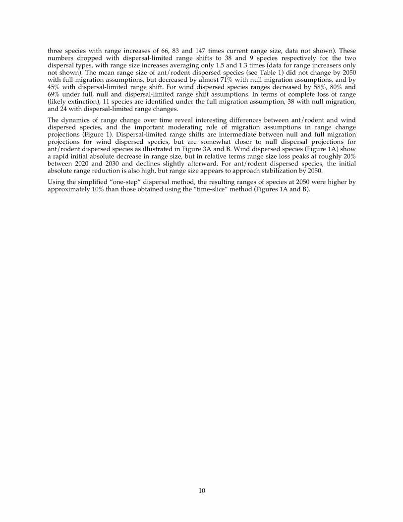
cells by blue). .......................................................................................................................................................... 12 Figure 3: The modeled potential distribution, of the Riverine Rabbit under current (top panels) and four

potential future (bottom panels) climate conditions, using bioclimate, food resources, vegetation

cover, land transformation and riparian habitat as determining factors of current range.................... 16 Figure 4: Modelled current ranges of Homopus signatus, Homopus signatus signatus and Homopus

signatus cafer excluding (a, b, c, respectively) and including (d, e, f, respectively) the forage resource

variable..................................................................................................................................................................... 18 Figure 5: Modelled future ranges of Homopus signatus, Homopus signatus signatus and Homopus

signatus cafer excluding (a, b, c, respectively) and including (d, e, f, respectively) the forage resource variable. Dark green areas indicate persistence in all four future climate scenarios with decreasing shades indicating persistence under fewer scenarios. Dark red areas indicate expansion in all 4

future scenarios with decreasing shades indicating expansion under fewer scenarios. ........................ 19 Figure 6: The components and interactions in a generalised savanna system. The ‘bowties’ are key

control points. Each linking arrow is represented by an equation. ............................................................ 21

Figure 7: Tree and grass trends, in the presence of fire, under a continuation of the current climate. ....... 26 Figure 8: Grazer and browser biomass trends under the current climate, but in the absence of carnivores

or elephants. ............................................................................................................................................................ 26

Figure 9: Carnivore response under continued normal climate. ....................................................................... 27

Figure 10: Plant response where elephants are included. ..................................................................................... 27

Figure 11: Elephant and medium-sized herbivore trends under the current climate. .................................... 28 Figure 12: Changes in production drivers given a B2 ( 550 ppm CO2 by 2080) scenario of climate change.

.................................................................................................................................................................................... 29 Figure 13: Changes in production drivers given a A2 (700 ppm CO2 by 2080) scenario of climate change.

.................................................................................................................................................................................... 29

Figure 14: Changes in vegetation structure given a B2 (Low) scenario of climate change. ........................... 30

Figure 15: Changes in vegetation structure given a A2 (High) scenario of climate change........................... 30

Figure 16: Changes in herbivore density given a B2 (low) scenario of climate change. ............................... 31 Figure 17: Changes in herbivore density given a A2 (high impact 700 ppm CO2) scenario of climate

change....................................................................................................................................................................... 31 Figure 18: A decision tree for selecting adaptation strategies for different surrogate species based on their

response to climate change (Adapted from Midgley et al in prep). ........................................................... 36

Figure 19: Operating costs for various park sizes. .................................................................................................. 40

Figure 20: Capital requirement for various park sizes. .......................................................................................... 41

vi

About AIACC Assessments of Impacts and Adaptations to Climate Change (AIACC) enhances capabilities in the developing world for responding to climate change by building scientific and technical capacity, advancing scientific knowledge, and linking scientific and policy communities. These activities are supporting the work of the United Nations Framework Convention on Climate Change (UNFCCC) by adding to the knowledge and expertise that are needed for national communications of parties to the Convention. Twenty-four regional assessments have been conducted under AIACC in Africa, Asia, Latin America and small island states of the Caribbean, Indian and Pacific Oceans. The regional assessments include investigations of climate change risks and adaptation options for agriculture, grazing lands, water resources, ecological systems, biodiversity, coastal settlements, food security, livelihoods, and human health. The regional assessments were executed over the period 2002-2005 by multidisciplinary, multi-institutional regional teams of investigators. The teams, selected through merit review of submitted proposals, were supported by the AIACC project with funding, technical assistance, mentoring and training. The network of AIACC regional teams also assisted each other through collaborations to share methods, data, climate change scenarios and expertise. More than 340 scientists, experts and students from 150 institutions in 50 developing and 12 developed countries participated in the project. The findings, methods and recommendations of the regional assessments are documented in the AIACC Final Reports series, as well as in numerous peer-reviewed and other publications. This report is one report in the series. AIACC, a project of the Global Environment Facility (GEF), is implemented by the United Nations Environment Programme (UNEP) and managed by the Global Change SysTem for Analysis, Research and Training (START) and the Third World Academy of Sciences (TWAS). The project concept and proposal was developed in collaboration with the Intergovernmental Panel on Climate Change (IPCC), which chairs the project steering committee. The primary funding for the project is provided by a grant from the GEF. In addition, AIACC receives funding from the Canadian International Development Agency, the U.S. Agency for International Development, the U.S. Environmental Protection Agency, and the Rockefeller Foundation. The developing country institutions that executed the regional assessments provided substantial in-kind support. For more information about the AIACC project, and to obtain electronic copies of AIACC Final Reports and other AIACC publications, please visit our website at www.aiaccproject.org.

vii

Summary Project Information

Regional Assessment Project Title and AIACC Project No. Impacts and adaptations to climate change by the biodiversity sector in southern Africa (AF 04).

Abstract Global climate change is predicted to have substantial impacts on South Africa’s unique and prolific biodiversity but consequences for conservation planning (adaptation) are poorly described. Five distinct technical innovations were developed to address the issue of adaptation of biodiversity to climate change. A case study approach was used to develop tools to better understand the likely response of biodiversity to climate change and how to incorporate this into strategic conservation planning. The economic implications of various adaptation option were developed to better understand what approaches are likely to be most affordable. The Proteaceae were used as an indicator group to investigate individual species response to climate change in the Cape Floristic Region. A ‘time-slice’ modelling approach was developed to investigate the migratory corridors needed for individual species to track climate change. Though most of the Protea species were projected to persist in the predicted climate of 2050, about 11% of species had no future habitat and 6% would need to move to new locations. Results from this study were used to review strategic conservation strategies for the region. In addition the data from this case study was used to investigate the use of economic models to better understand the cost effectiveness of various adaptation options, including expanding the reserve network, promotingconservation outside of the reserve network (matrix management), facilitated dispersal, ex-situ preservation or doing nothing. Tools to investigate the impacts of climate change on single animal species, based on, changes in food species availability was investigated for two species, the highly endangered riverine rabbit (Bunolagus monticularis) and padloper tortoise (Homopus singnatus). Climate change was found to increase the likelihood of extinction of the riverine rabbit, whilst it appears that the padloper tortoise appears far better able to persist, facilitating adaptation. Modelling approaches to investigate key functional properties (tree cover, fire frequency, grass and browse production and carrying capacity for major guilds of erbivores and carnivores) were investigated for the north-eastern lowveld savanna. This approach predicted slight increases in woodiness in the coming century. Elephant density and fire were found to be important variables controlling vegetation dynamics. Learning from the project was consolidated into a training manual that was presented as a short course to SADC delegates and is available as a web based training module. The learning was also used to influence South Africa’s UNFCCC COP9 negotiations.

Administering Institution

CSIR, Division of Water, Environment and Forest Technology (Environmentek), Pretoria, South Africa

Participating Stakeholder Institutions South African National Parks Board, South Africa; South African Department of Environmental Affairs and Tourism, South Africa

Countries of Primary Focus South Africa as primary focus, with relevance to the SADC region

Case Study Areas Fynbos biome, Western Cape Province, South Africa Succulent Karoo, West Coast of South Africa and Southern Namibia

viii

North Eastern Lowveld savanna, Limpopo and Mpumalanga Provinces, South Africa

Systems and Sectors Studied Biodiversity and Conservation sector Biodiversity at the species and ecosystem level in the: Fynbos (Cape Floral Kingdom) Succulent Karoo Savanna regions of the North Eastern Lowveld.

Groups Studied The study was primarily of the conservation implementation community and how it could adapt the systematic planning process to accommodate climate change. In South Africa conservation is represented through the National Department of Environmental Affairs and Tourism, which includes the National Parks Board and South African National Biodiversity Institute (SANBI) as well as through Provincial Departments of the Environment and in some cases Provincial Parks Boards.

Sources of Stress and Change The main sources of stress investigated were changes in mean monthly precipitation, temperature and evapo-transpiration. In addition changes in CO2 levels where also considered.

Project Funding and In-kind Support AIACC: US$195,000 grant; SANBI (NBI): US$ 57,000 in-kind contribution; CSIR: US$450,000 in-kind contribution in parallel research; National Parks Board, South Africa: US$ 5,000 in-kind contribution; University of Pretoria/ Wits/ Stellenbosh: US$ 25,000 in-kind contribution.

Investigators Principal Investigator: Dr Robert (Bob) J. Scholes, CSIR, Division of Water, Environment and Forest Technology (Environmentek), P.O. Box 395, Pretoria 0001, South Africa. Email: bscholes@csir.co.za Other Investigators: Graham von Maltitz, CSIR, South Africa; Dr Martin de Wit, CSIR, South Africa; Jenny Cooper, CSIR, South Africa; Caroline Geldenblom, CSIR, South Africa; Anthony Letsoalo, CSIR, South Africa; Sally Archibald, CSIR, South Africa; Belinda Reyers, CSIR, South Africa; Dr Albert van Jaarsveld, University of Stellenbosch (originally University of Pretoria), South Africa; Dr Barend Erasmus, University of the Witwatersrand (originally University of Pretoria), South Africa; Dr Guy Midgely, SANBI, South Africa; Greg Hughes, SANBI, South Africa; Dr Mike Rutherford, SANBI, South Africa.

ix

Executive Summary

Research problem and objectives The impetus for this project came out of work done in the late 1990’s under the umbrella of South African country studies on vulnerability to climate change (South Africa, 2000). One of the ‘sectors’ identified in those studies as being particularly at risk in South Africa was biodiversity. When the results of the relatively crude analyses done at that time were presented to officials in the leading conservation agencies, they were extremely concerned, and immediately asked the question ‘What should we do about it?’ The researchers involved in the impact studies had no ready answer. When we went back to the literature, we found that apparently nobody had any good answers to that question. The biodiversity conservation advocacy groups had focused on the issue of mitigating climate change because of its potential impacts, but had not really grappled with the practical steps that conservation authorities might take if faced with the actuality of climate change. However, the IPCC Third Assessment Report (2001) had made it clear that due to inertia in the climate system, further climate change was now inevitable, regardless of the mitigation strategy that was put in place. Therefore adaptation is essential and non-negotiable. Mitigation actions remain critically important, because they determine the rate and final extent of climate change, but they are no longer an alternitive to adaptation. The community of South African researchers, which had developed around the climate change impact work, therefore came together to work out the next steps, and fortuitously, the Analysis of Impacts and Adaptation to Climate Change (AIACC) funding opportunity arose at the same time. It soon became clear that the key next steps were:

1. to develop a conceptual framework within which to consider the adaptation of biodiversity to climate change; and

2. to develop, test, and transfer a set of tools for the use of officials with a mandate and responsibility for biodiversity conservation to apply in the analysis of response options.

The objectives of this project were to: 1. Develop and test methods to project the dynamic response of biodiversity to climatic change. 2. Develop conservation planning tools for the prioritization of conservation planning in an

environment, which is non-static, as a result of climate and land use change. 3. Evaluate, in terms of economic costs and effectiveness, adaptation options for biodiversity

conservation when faced with climate change and a fragmented landscape. This will involve the development of a cost-effectiveness evaluation method, and testing and illustrating it using diverse southern African examples as to how the climate change induced mitigation of biodiversity can be incorporated in the new move towards strategic conservation planning.

4. Collate, assess, summarise and publicise the information relating to potential impacts on South African biodiversity from the combination of climate and land use change in the 21st century.

5. Advance the field of dynamic biodiversity conservation and develop capacity in both the research and management communities to address climate change issues in a proactive and effective way.

This study is therefore about the vulnerability of aspects of biodiversity to climate change, and not per se about the resultant vulnerability of human populations dependent on biodiversity. That is a second step in the analysis that we did not take. By doing so, we are not expressing an opinion on the debate about whether the value of biodiversity is solely utilitarian (ie based on its usefulness to humans) or whether it is intrinsic (valuable in its own right). We are simply saying that before we can estimate the impacts on human societies, we must understand the impacts on organisms and ecosystems. In the context of South Africa, we take it as given that biodiversity has a large value to society, since society devotes considerable resources to its protection.

x

The first major innovation which this project introduced relative to prior work in South Africa was the view climate change as a transient (continuous) phenomenon, rather than as a equilibrium (step change) phenomenon. The key issue in autonomous adaptation of organisms to climate change is seldom whether a suitable climate exists in future scenarios, but whether the organisms can move at a sufficient rate to keep up with the changing spatial distribution of their preferred environment, and thus avoid range loss and increasing stochastic likelihood of extinction. To achieve this, we had to develop dynamic niche modelling tools, and approaches to doing conservation estate optimisation for non-stable climates. The second innovation was to introduce non-climate ‘global change’ factors into the analysis. Species need to move through a complex, fragmented landscape, with more-or-less hospitable or inhospitable attributes. Substrate, land use, climate change and other pressures are acting simultaneously on the organisms. The third innovation was to move beyond very simplistic approaches to niche envelope modelling, to more sophisticated ones involving more robust statistical approaches, multiple (but independent) dimensions, including niche dimensions such as substrate and the presence of synergistic species. Advances in computational power made it possible for us to perform such analyses on an unprecedented large number of species, making a ‘guild’ or ‘representative species’ approach largely unnecessary. We also developed approaches to modelling the functional attributes of biodiversity under climate change, rather than the purely compositional aspects. In other words, we addressed the questions like: what will the population sizes and productivities be in the future? The fourth innovation was to view biodiversity conservation as a continuum from strict protection in formal protected areas, through off-reserve protection on private lands, used to varying degrees fro other purposes, right through to ex situ protection in zoos, gardens or even gene banks. Conservation then becomes not a yes/no option, but a range of degrees of success and risk. At the same time, conservation strategies need not be limited to one option (proclaim a protected area), but consist of a portfolio of actions with different attributes, and the optimisation lies in the mix of the portfolio. The fifth innovation was to couch the adaptation strategies in an economic framework. There are many technical solutions, but in the real world, what is implementable is strongly influenced by cost. We did not try to do a strict cost-benefit analysis (ie answer the question: how much should society spend overall to conserve biodiversity?) but we did make progress towards answering the question: how much biodiversity do you protect for what cost?

Approach Three case studies were used to develop and test tools and methodologies for better understanding the response of species and ecosystems to the predicted impacts of climate change. In the case of our Fynbos case study, the results were used to investigate how to configure conservation areas to best achieve biodiversity conservation in a dynamic environment. Barring evolution, biological organisms effectively have four possible response options to changes in climate, and based on this we have grouped organisms into the following functional groups:

1. Persisters: These species that have the climate tolerance for the new climate. 2. Obligatory dispersers: These species have to move to now areas that maintain their current

climate envelope in the future. 3. Expanders: These are species that will find new habitats based on the new climates i.e. they can

expand into new climatic envelopes that where not previously available. 4. No hopers: If the species cannot do one of the above then they will become extinct. In other

words the future climate holds no suitable climatic envelopes for them to persist. Based on the response options available to individual species, the following potential adaptation options were identified:

• Do nothing (i.e. maintain the current conservation strategy).

• Reconfiguration of reserve system.

xi

• Matrix management. i.e. managing the biodiversity in areas outside of reserves.

• Translocation of species in to new habitats.

• Ex-situ conservation.

An economic analysis was undertaken on the costs of different conservation option based on the results from the Fynbos case study.

Scientific findings Rapid advances in individual species dispersion modelling techniques between our conceptualization of the project, and actual implementation, allowed us to develop methodologies based on individual species response, rather than habitat level responses. Initial models, though powerful, were very data intensive to parameterise. These models proved too complex to apply to large numbers of individual species. A simpler grid based approach was developed that made far simpler assumption on dispersal distances in any time period. Grids of 1 x 1 minute cells (average 1.85 x 1.55 km along their sides, area approximately 2.87 km2) were used, and each cell was parameterised in terms of climatic suitability and suitability in relationship to the extent of land transformation. Individual species were allocated dispersal distances per time period based on their seed dispersal biology. A time slice methodology was developed to predict individual species dispersal response to predicted climate change. The data rich Proteaceae distribution data was used to test the model for the Fynbos biome of the Western Cape. Wind dispersed species were given allowed to disperse three grid cells per 10 year time slice, whilst and dispersed species were limited to the distance of one grid cell. The model was able to identify important distribution corridors that would allow obligatory disperser species to track climate change. Though most of the Protea species were projected to persist in the predicted climate of 2050, about 11% of species had no future habitat and 6% would need to move to new locations. Results from this study were used to review strategic conservation strategies for the region. In addition the data from this case study was used to investigate the use of economic models to better understand the cost effectiveness of various adaptation options, including expanding the reserve network, promoting conservation outside of the reserve network (matrix management), facilitated dispersal, ex-situ preservation or doing nothing. Models to understand likely extinction of individual animal species, based on the impacts that climate change would have on habitat structure and food plants was investigated for two karoo species, the highly endangered riverine rabbit (Bunolagus monticularis) and the padloper tortoise (Homopus singnatus). The climate change scenarios investigated were found to increase the likelihood of extinction of the riverine rabbit, whilst it appears that the padloper tortoise will be able to persist, which will facilitate adaptation. Modelling approaches based on relatively simple procedure, based on empirical equations, for predicting the key functional properties of savannas (tree cover, fire frequency, grass and browse production and carrying capacity for major guilds of herbivores and carnivores) were developed for the north-eastern lowveld savanna. The modelling considered both the impacts of temperature and rainfall, as well as changes in CO2 on relative competitive advantage of grasses and trees. This approach predicted slight increases in woodiness in the coming centuary. Elephant density and fire were found to be important variables controlling vegetation dynamics. In determining the economic costs of adaptation options we made the up front assumption that benefits should be measured as the number of species that would be conserved using different adaptation strategies. This decision was made instead of attempting to derive a total economic value of saved species. Total economic valuation was discarded because a) there was no objective way to value of non-use values, b) many non-consumptive use values cannot be objectively distributed between different biota in any specific habitat and c) we did not want to find solutions based purely on current human values. The economic modelling found that the cost of expanding the conservation network was inversely related to the size of conservation areas. In most circumstances managing the biodiversity in farmlands outside of conservation area, what we termed matrix management, was found to be a more economically viable option than expansion of the reserve network. The exception to this is when land has the potential for high value crops such as grapes. In these circumstances placing the land in a reserve may be more economically viable provided that the area is relatively large. In all other situations a contractual

xii

relationship where the farmer is paid not to farm and is compensated at the opportunity cost of the lost production is a more economically viable option than establishing a formal reserve. Lower cost options that encourage biodiversity-friendly farming are also available for less critical areas. Ex-situ conservation will be required for species that have no suitable habitats in the future. The costs of ex-situ conservation cannot be directly compared with conventional conservation as it has different objectives. Due to uncertainty of climate change scenarios and poor understandings of how individual species will respond, ex-situ conservation should be considered as a safety strategy to protect extinction for all species. Strategies for individual species need to differ based on the adaptive capacity of any species. It is possible to re-configure protected areas either through reserves or matrix management to provide greater protection of biodiversity given climate change. There will still remain a necessity to intervene for specific species that will either have no available dispersal corridors and which will need assistance in migration, or which have no future habitat (in the 50 to 100 year time frame) and that will need ex-situ conservation until the impacts of climate change reverse. Simple strategies such as the protection of potential migratory corridors along environmental gradients are confirmed.

Capacity building outcomes and remaining needs A number of researchers from national research institutes and universities gained capacity in climate change and the vulnerability and adaptation options of biodiversity through direct involvement in the project. In addition, with the aid of a supplementary AIACC grant, we were able to present a training course to researches from 10 SADC counties and a number of South African institutions. Parts of our findings are already being used in postgraduate training. We have developed our training material into a Web Based training module that will be housed at the University of the Western Cape and will be available as a self learning module as well as being used as a component of postgraduate training module (http://planet.uwc.ac.za/nisl/AIACC).

National communications, science-policy linkages and stakeholder engagement A memorandum, based on AIACC activities in project AF04, was presented at a sitting of the National Cabinet of South Africa for consideration during 2004, and was revised in order to form the basis for a briefing paper for national team’s UNFCCC COP9 negotiations. This memo indirectly precipitated the increase in urgency in governmental concern in climate change threats to South Africa, and contributed to informing its negotiating position. Two of the core research team Dr have been actively involved in representing South Africa on IPCC WG panels in the following capacities:

• Dr Bob Scholes: IPCC WG3 group on agriculture

• Dr Guy Midgley IPCC WG2 on ecosystems. In addition both Dr Scholes and Dr Midgley are part of the South African negotiating team for UNFCCC meetings.

Policy implications and future directions National issues

1. Systematic biodiversity conservation needs to plan for change, and not assume that the future will be like the past.

2. Conservation biologists need to break from the old paradigm that species should only be located in areas where they historically occurred

3. The protected area system can be configured to improve the protection it provides against climate change, including making provision for species movement.

4. Given current economic and land use realities, it is unlikely that the protected area system can be sufficiently reconfigured to achive species conservation targets. Conservation authorities

xiii

therefore need to maximize off reserve conservation, which is both cost effective and provides more spatial options.

Regional issues 1. Transfrontier movement of biodiverisity will be important given climate change. 2. As a result, regional strategic conservation planning needs to consider park configuration to

best protect against the impacts of climate change. 3. Regional capacity building, especially in SADC countries other than South Africa is needed for

these countries to develop sufficient capacity to deal with adaptations to climate change. Global issues

1. The cost to biodiversity, in both utilitarian and intrinsic terms, of anthropogenic climate change is high, and needs to be better understood and communicated.

Future directions and research needs: 1. Consider the impacts of biodiversity loss on income and livelihood strategies 2. Move from case studies to national strategic assessment 3. Conduct sub-regional assessment of the level of threat 4. Undertake detailed studies on threatened genera 5. Build capacity in other SADC countries

1

1 Introduction The AIACC project on adaptation of biodiversity to climate change to the biodiversity sector in Southern Africa.

The impetus for this project came out of work done in the late 1990’s under the umbrella of South African country studies on vulnerability to climate change (South Africa, 2000). One of the ‘sectors’ identified in those studies as being particularly at risk in South Africa was biodiversity. When the results of the relatively crude analyses done at that time were presented to officials in the leading conservation agencies, they were extremely concerned, and immediately asked the question ‘What should we do about it?’ The researchers involved in the impact studies had no ready answer. When we went back to the literature, we found that apparently nobody had any good answers to that question. The biodiversity conservation advocacy groups had focused on the issue of mitigating climate change because of its potential impacts, but had not really grappled with the practical steps that conservation authorities might take if faced with the actuality of climate change. However, the IPCC Third Assessment Report (2001) had made it clear that due to inertia in the climate system, further climate change was now inevitable, regardless of the mitigation strategy that was put in place. Therefore adaptation is essential and non-negotiable. Mitigation actions remain critically important, because they determine the rate and final extent of climate change, but they are no longer an alternate to adaptation. The community of South African researchers which had developed around the climate change impact work therefore came together to work out the next steps, and fortuitously, the Analysis of Impacts and Adaptation to Climate Change (AIACC) funding opportunity arose at the same time. It soon became clear that the key next steps were:

1. to develop a conceptual framework within which to consider the adaptation of biodiversity to climate change; and

2. to develop, test, and transfer a set of tools for the use of officials with a mandate and responsibility for biodiversity conservation to apply in the analysis of response options.

The objectives of this project as per the original proposal were to: 1. Develop and test methods to project the dynamic response of biodiversity to climatic change 2. Develop conservation planning tools for the prioritization of conservation planning in an

environment which is non-static, as a result of climate and land use change 3. Evaluate, in terms of economic costs and effectiveness, adaptation options for biodiversity

conservation when faced with climate change and a fragmented landscape. This will involve the development of a cost-effectiveness evaluation method, and testing and illustrating it using diverse southern African examples as to how the climate change induced mitigation of biodiversity can be incorporated in the new move towards strategic conservation planning.

4. Collate, assess, summarise and publicise the information relating to potential impacts on South African biodiversity from the combination of climate and land use change in the 21st century.

5. Advance the field of dynamic biodiversity conservation and develop capacity in both the research and management communities to address climate change issues in a proactive and effective way.

The conceptual framework that we developed has several important features. Firstly, it is loosely based on the concept of ‘vulnerability’, in other words, the interaction of an impact of a given magnitude, with a response unit which has a particular coping capacity with respect to that impact. Vulnerability theory has been developed in the context of units of human organisation as the ‘responding unit’, and is particularly associated with a school of practice known as the ‘Livelihoods’ approach. The Livelihoods approach focuses on the family as a response unit, and take a holistic view of factors that impact on the viability of that unit. It also views the family as an extremely adaptive unit, which does not simply passively contend with changes in its environment, but actively and continuously adapts to its environment, and often adapts its environment to its needs.

2

In this study, aspects of biodiversity are the response unit. Biodiversity is conventionally seen as having several levels of organisation, ranging from the gene up to ecosystems. Our focus was at two levels: that of the species (ie set of populations of individuals with sufficient genetic similarity to allow reproduction), and that of the ecosystem (a set of interacting organisms of different species, within an environment with a defined range of abiotic attributes, and usually a defined spatial extent). Clearly, some of the vulnerability concepts can be adopted unchanged from the human system context, but others cannot. In particular, it is not possible to impute to biological systems the kinds of rational and preemptive actions that we expect from human systems. This study is therefore about the vulnerability of aspects of biodiversity to climate change, and not per se about the resultant vulnerability of human populations dependent on biodiversity. That is a second step in the analysis that we did not take. By doing so, we are not expressing an opinion on the debate about whether the value of biodiversity is solely utilitarian (ie based on its usefulness to humans) or whether it is intrinsic (valuable in its own right). We are simply saying that before we can estimate the impacts on human societies, we must understand the impacts on organisms and ecosystems. In the context of South Africa, we take it as given that biodiversity has a large value to society, since society devotes considerable resources to its protection. There is a significant biodiversity-based economic sector in southern Africa, including both the informal and formal sectors that rely on the products of natural ecosystems to generate value (for instance, wood, craft materials and medicines collected from the wild, and natural pasturage for domestic and wild livestock), and increasingly a booming service sector built on nature-based tourism. The ‘biodiversity sector’ is not explicit in national accounts, partly because much of it is in the informal sector, and partly because the formal part of it is distributed across the tourism, agriculture, forestry and fisheries sectors. Satellite accounts exist for the tourism sector overall, amounting to Billions of US$ per year, of which about half is directly attributable to nature based tourism. The first major innovation which this project introduced relative to prior work in South Africa was the view climate change as a transient (continuous) phenomenon, rather than as a equilibrium (step change) phenomenon. The key issue in autonomous adaptation of organisms to climate change is seldom whether a suitable climate exists in future scenarios, but whether the organisms can move at a sufficient rate to keep up with the changing spatial distribution of their preferred environment. To achieve this, we had to develop dynamic niche modelling tools, and approaches to doing conservation estate optimisation for non-stable climates. The second innovation was to introduce non-climate ‘global change’ factors into the analysis. Species need to move through a complex, fragmented landscape, with more-or-less hospitable or inhospitable attributes. Substrate, land use, climate change and other pressures are acting simultaneously on the organisms. The third innovation was to move beyond very simplistic approaches to niche envelope modelling, to more sophisticated ones involving more robust statistical approaches, multiple (but independent) dimensions, including niche dimensions such as substrate and the presence of synergistic species. Advances in computational power made it possible for us to perform such analyses on an unprecedented large number of species, making a ‘guild’ or ‘representative species’ approach largely unnecessary. We also developed approaches to modelling the functional attributes of biodiversity under climate change, rather than the purely compositional aspects. In other words, we addressed the questions like: what will the population sizes and productivities be in the future? The fourth innovation was to view biodiversity conservation as a continuum from strict protection in formal protected areas, through off-reserve protection on private lands, used to varying degrees fro other purposes, right through to ex situ protection in zoos, gardens or even gene banks. Conservation then becomes not a yes/no option, but a range of degrees of success and risk. At the same time, conservation strategies need not be limited to one option (proclaim a protected area), but consist of a portfolio of actions with different attributes, and the optimisation lies in the mix of the portfolio. The fifth innovation was to couch the adaptation strategies in an economic framework. There are many technical solutions, but in the real world, what is implementable is strongly influenced by cost. We did not try to do a strict cost-benefit analysis (ie answer the question: how much should society spend overall to conserve biodiversity?) but we did make progress towards answering the question: who much biodiversity do you protect for what cost?

3

The AIACC biodiversity adaptation project used three broad case studies to advance this work. The first was located in the extreme southwestern tip of South Africa, the ‘Fynbos biome’, which has very high levels of endemism in a very small area. The landscape is highly fragmented by both topography and land use, and has a unique (for southern Africa) winter rainfall regime. It also has an uniquely detailed plant distribution dataset, especially for the family Proteaceae. This case study was therefore used to explore conservation planning algorithms under non-stable climates, and to develop the dynamic species movement models. The second case study area was the succulent Karoo, on the west coast of Southern Africa. It also has a high endemic plant biodiversity, and a climate that is projected to change significantly in this century. This was a test area for a much sparser dataset, and for applying advanced niche modelling techniques involving substrate specificity, and inter-species relationships. The final case study area was the north-eastern Lowveld of South Africa, a savanna area famous for its large mammal wildlife populations. We used this to develop and test functional approaches to climate change impact modelling. The project ran a training course to disseminate knowledge gained to other practitioners and policy makers in the Southern African Region (SADC).

4

2 Characterization of Current Climate and Scenarios of Future Climate Change

2.1 Activities Conducted This project did not develop characterization models for climate, but rather relied on the existing Agricultural Atlas climate surface dataset (Schulze et al., 1999) at a resolution of 1 minute by 1 minute (~1.6 km at this latitude) to represent current climate along with recently constructed rainfall surfaces (Lynch, 2003). Future (~2050 and ~2080) climate predictions were produced by perturbing the current climatic data with anomalies derived from climatic simulations produced by the HADCM3 General Circulation Model using the A1F1, A2, B1 and B2 IPCC SRES scenarios (Nakicenovic & Swart 2000) in accordance with guidelines for climate impact assessment (IPCC-TGCIA 1999) utilizing a technique described by (Hewitson, 2003).

5

3 Socio-Economic Futures 3.1 Activities Conducted This study did not specifically conduct research on socio-economic futures. The principle investigator (Dr Bob Scholes) was, however, intimately involved in future scenario development as a component of the Millennium Assessment project that was run in parallel to this project (See Scholes and Biggs 2004 chapter 3).

6

4 Impacts and Vulnerability 4.1 Activities Conducted Three case studies were used as a mechanism to develop and test different tools for understanding impacts and vulnerability of biodiversity to climate change. A full literature review was conducted on existing methods and studies. This has been consolidated into a review paper (Midgley et al in prep).

4.2 Description of Scientific Methods and Data Three case studies where conducted as a mechanism to develop and test various approaches to predicting impacts of both individual species and functional groups of species to climate change. Each case study is presented separately below. The case studies were: 1. Use of the Proteaceae in the Fynbos (Cape Floral Kingdom) to develop time slice models to

investigate individual species responses to migration as a consequence of climate change. 2. Use of two animal species in the Succulent Karoo to investigate if they can track changes in food

sources as a consequence of climate change. 3. Use the savanna of the north eastern lowveld to investigate modelling tools for investigating the

response of functional groups to climate change. Details of methods and results are presented for each case study Results are presented with each case study.

4.2.1 Advances in bioclimatic niche based-modelling We addressed the first, second and third innovations mentioned above in our studies of the potential responses of components of biodiversity to global changes in the Fynbos and Succulent Karoo Biomes. In these studies we aimed to generate biologically and ecologically more realistic projections of temporally specific species range responses to climate change (in annual or decadal time steps) as opposed to static step change projections often carried out in such studies, in addition to taking into account simple assumptions of species potential migration rates and the presence of “synergistic species”. Study methods for these studies are given in detail in the attached manuscripts that have been accepted and submitted for publication or are in preparation. Possibly the most innovative part of this work was to develop a spatially explicit population level modelling approach that could be applied at a regional scale. However, we discovered that the parameterization requirements of this model exceeded the information base for almost all species. We therefore reverted to a simpler diffusion-type approach to model species potential range shifts, as this provides a tool that is more generally applicable with current information available to the potential users of this tool. We have termed this approach “time slice modelling” as described in Midgley et al (submitted). We are continuing to develop and refine the population level approach independently of the AIACC program.

4.2.2 Climate scenarios We used the same approach to climate scenario generation for the Fynbos and Succulent Karoo studies. The Agricultural Atlas climate surface dataset (Schulze et al., 1999) at a resolution of 1 minute by 1 minute (~1.6 km at this latitude) was used to represent current climate along with recently constructed rainfall surfaces (Lynch, 2003). Future (~2050 and ~2080) climate predictions were produced by perturbing the current climatic data with anomalies derived from climatic simulations produced by the HADCM3 General Circulation Model using the A1F1, A2, B1 and B2 IPCC SRES scenarios (Nakicenovic & Swart 2000) in accordance with guidelines for climate impact assessment (IPCC-TGCIA 1999) utilizing a technique described by (Hewitson, 2003). Owing to little experimental work having been undertaken on local indigenous plant species to guide in the choice of bioclimatically limiting variables, a suite of potential variables was selected for use. These included summer, winter and annual averages of precipitation, mean temperature, potential evapotranspiration, growing degree-days and heat units as well as the highest maximum and the lowest

7

minimum temperatures. Potential evapotranspiration estimates were calculated using the FAO 56 Penman Monteith combination equation (Allen et al. 1998). Winter temperature is likely to discriminate between species based on their ability to assimilate soil water and nutrients, and continue cell division, differentiation and tissue growth at low temperatures (lower limit), and chilling requirement for processes such as bud break and seed germination (upper limit). Potential evaporation discriminates through processes related to transpiration-driven water flow through the plant, and xylem vulnerability to cavitation and water transport efficiency.

4.3 Results

4.3.1 Fynbos Biome case study: Time slice models for species range shifts as constrained by dispersal assumptions

4.3.1.1 Scientific method and data

We considered the western part of the Cape Floristic Region extending to 20°48’ E and to 31°53’ S where it encompasses Fynbos communities. This is the part of the Cape Floristic Region that is most vulnerable to anthropogenic climate change (Midgley et al. 2002). We used a grid of 1 x 1 minute cells (average 1.85 x 1.55 km along their sides, area approximately 2.87 km2) because cells this size are small enough to be useful for practical planning and yet sufficiently large to be appropriate for modelling climate ((Pearson & Dawson, 2003)). Habitat transformation and changing land use compound the effects of climate change (e.g. (Peters, 1991; Peters & Darling, 1985; Travis, 2003)). Based on information from CSIR (1999), we estimated that transformation of habitat to an unsuitable state has exceeded 66% of the unit grid cell area for 6036 of the one-minute grid cells. The distribution data for the Proteaceae was set to zero for these cells. In contrast, we estimated that there was adequate existing protection for 1525 of the grid cells in statutory protected areas ((Rouget et al., 2003)). Species’ distribution data were taken from the Protea Atlas Project (PAP) database, which contains field-determined species presence and absence at more than 60,000 georeferenced sites. This is an unusually thorough sampling of localities totalling more than 250,000 species records for 340 taxa http://protea.worldonline.co.za/default.htm). Climate data were interpolated for the one-minute grid ((Schulze, 1997)). Future projections were based on Schulze and Perks ((1999)), according to the 2050 projections for the region from the General Circulation Model HadCM2 (http://cera-www.dkrz.de/IPCC_DDC/IS92a/Hadley-Centre/Readme.hadcm2), using IS92a emissions assumptions for CO2 equivalent greenhouse-gas concentrations, and excluding sulphate-cooling feedback. Soil categorization relating to fertility (high, medium, and low), pH (acid, neutral, and basic), and texture (sand and clay) were derived for the one-minute grid by interpolation of regional geology maps (R. Cowling and A. Rebelo, personal communication). Information on nomenclature and on species’ dispersal modes was taken from Rebelo ((2001)). Bioclimatic and Dispersal Time-slice Modelling

Expected distributions were modeled separately for individual Proteaceae species on the one-minute grid (Table 1) by considering both the changing environmental suitability for each species (depending primarily on climate: (Midgley et al., 2003)) and its particular dispersal constraints (depending primarily on the dispersal agent). We made time-slice distribution models for each species for each of the years 2000, 2010, 2020, 2030, 2040, and 2050. Distributions for the year 2000 were also modeled because the original sampling did not include all grid cells. Dispersal assumptions

Dispersal distances were assumed to be a maximum of one cell per time slice for ant- and rodent-dispersed species (which may be an overestimate), and a maximum of three cells per time slice for wind-dispersed species (corresponding to at least 4 km in 10 years or 400 m in 1 year, which may be considered long distance dispersal: (Cain et al., 2000)). According to these models, 282 of the 316 Proteaceae species modeled would be expected to persist from 2000 to 2050 within the region, occupying 17,677 cells with a total of 1,304,019 occurrences (ignoring habitat transformation).

8

Planning Framework and Goals

We identified important areas for conservation by using the planning framework described by Cowling and Pressey ((2003): their Table 1). Our method relates most directly to their stage 7: the selection of additional conservation areas to extend the existing protection . Continuous climate change response: the concept of “Dispersal Chains” for species

Our primary criterion for choosing areas was to minimize the distances species would be forced to disperse in order to promote each species’ probability of persistence. For some species, the minimum distance will be zero. We identified these persistence areas from a pattern of overlap of grid cells, where species are expected to continue to occur within the same cells in all six of our future time-slice models (without any implication for past or future persistence beyond the modeled time slices). Not all species can remain in persistence areas because habitat becomes unsuitable, so for the remaining (obligate disperser) species that will have to track the changing climate we sought to give them shortest possible dispersal distances. We identified these dispersal corridors from a pattern of chains of grid cells across time-slice models, which provided connectivity, either as stepping stones or as more continuous corridors of suitable areas, linked in space and time within the constraints of our dispersal models. We identified dispersal chains of grid cells for a species by (1) finding suitable cells within successive time slices that lie within the maximum permitted dispersal step (of one or three grid cells, as appropriate) from previously suitable cells (Fig. 1) and (2) reiterating to find all such dispersal chains linking all time slices. In practice, the search for chains (Fig. 1) started from the 2050 time slice and worked backward to earlier time slices, because it was more efficient as distributions generally tend to become narrower over time. For a dataset of this size, there are so many chains that it is impractical to store and select among them all on a personal computer. Therefore we stored a sample of up to 1000 of the shortest chains found for each species for the area-selection procedure. This sample size should be sufficiently large to increase efficiency by allowing the discovery of overlapping chains among the species during area selection. Less desirably, many of the chains for any one species overlapped in part, or even in total, because the dispersal jumps can occur between the same cells but between more than one pair of time slices. To ensure that we end up with 35 independent chains for each species, we retained only completely nonoverlapping chains for the subsequent area-selection procedure. Which particular chains are selected first for the sample will affect which subsequent chains are found to be nonoverlapping. The effect of this is not addressed here. Classical approaches in conservation biology: Area Selection

Our secondary criterion for choosing areas was to minimize the total cost to society required to represent all the species ((Faith & Walker, 1996; Williams et al., 2003)). Resources are limited, so minimizing the cost should reduce conflicts between conservation needs and society’s other needs. We used land area as a surrogate for cost because no more appropriate data were available. Cost-efficiency was achieved by selecting cells that are part of the most highly complementary sets of chains among species. The chains were sorted by length within the sample for each species so that the shorter chains could be chosen preferentially. The area-selection procedure consisted of three stages. First, for the species that have a maximum of 35 or fewer chains, we selected all of the unprotected cells within these chains. Selecting these goal-essential chains first is a modification of a procedure within popular heuristic algorithms that has been proven to increase efficiency. For species that could not achieve 35 nonoverlapping dispersal-constrained chains, we could have included other cells from partly overlapping chains as conservation areas. We did not do this, but these cells could be added by backtracking to search again for partly overlapping chains. Second, for species that did not reach the goal of 35 chains but could have, we identified all chains that were represented in part within the existing protected areas, or within the goal-essential cells selected at the first stage. We then selected cells to complete these chains for up to 35 chains per species. Tests with the obligate disperser species alone showed that including this stage increased area efficiency by 5-6%. Third, for any remaining species that still did not reach the goal of 35 chains (i.e. those that could reach 35 chains but did not have chains partly represented within the existing protected areas), we used an iterative heuristic algorithm to select a set of complementary areas. The chains-search and area-selection methods were written in the C programming language and implemented within the Worldmap software (see http://www.nhm.ac.uk/science/projects/worldmap/index.html).

9

4.3.1.2 Fynbos Biome results

Querying dispersal assumptions

Species range changes of modeled Proteaeceae at 2050 varied widely, with the greatest variability shown under the full migration assumption. With full migration, 255 species overall showed range decreases, and 81 showed increases, compared with 47 species that showed a range increase given dispersal-limited range shifts, and, by definition, no species with null migration assumptions (Table 1). Overall, mean species range sizes were reduced by climate change in 2050 by 29% with full migration, by 75% with null migration, and by an intermediate figure of 58% assuming dispersal-limited range shift (Table 1).

2000 (current modeled)

2050 full migration

2050 null migration

2050 dispersal-limited

Range size (# pixels)

All species (n = 336)

1898 (108) 1349 (165) 466 (54) 802 (104)

Wind dispersed (n = 134)

2364 (179) 982 (111) 478 (48) 724 (73)

Ant/rodent dispersed

(n = 202) 1590 (131) 1592 (264) 458 (84) 878 (166)

Range increasers (# species)

Wind dispersed 19 - 10

Ant/rodent dispersed 62 - 38

Extinctions (# species)

Wind dispersed 2 11 5

Ant/rodent dispersed 9 27 18

Table 1: Impacts of climate change on the range size, range increase and extinctions of Cape Proteaceae (climate scenario based on (Schulze & Perks, 1999), according to the 2050 projections for the Cape Floristic Region from the General Circulation Model HadCM2). Range shift results differed between ant/rodent and wind dispersed species. Overall, wind dispersed species had 49% larger modelled ranges under current climate conditions than did ant/rodent dispersed species. Under full migration assumptions, 62 of the 134 ant/rodent dispersed species showed mean range increases by 2050 of 13 times their current range size (Table 1). This average was strongly skewed by 5 species that increased range by more than 20 times, two species by more than 40 times and 1 species by almost 450 times, with the remainder showing relatively small range increases. Only 19 of 202 wind dispersed species showed increases in range, averaging 17.5 times their current range (but dominated by

10

three species with range increases of 66, 83 and 147 times current range size, data not shown). These numbers dropped with dispersal-limited range shifts to 38 and 9 species respectively for the two dispersal types, with range size increases averaging only 1.5 and 1.3 times (data for range increasers only not shown). The mean range size of ant/rodent dispersed species (see Table 1) did not change by 2050 with full migration assumptions, but decreased by almost 71% with null migration assumptions, and by 45% with dispersal-limited range shift. For wind dispersed species ranges decreased by 58%, 80% and 69% under full, null and dispersal-limited range shift assumptions. In terms of complete loss of range (likely extinction), 11 species are identified under the full migration assumption, 38 with null migration, and 24 with dispersal-limited range changes. The dynamics of range change over time reveal interesting differences between ant/rodent and wind dispersed species, and the important moderating role of migration assumptions in range change projections (Figure 1). Dispersal-limited range shifts are intermediate between null and full migration projections for wind dispersed species, but are somewhat closer to null dispersal projections for ant/rodent dispersed species as illustrated in Figure 3A and B. Wind dispersed species (Figure 1A) show a rapid initial absolute decrease in range size, but in relative terms range size loss peaks at roughly 20% between 2020 and 2030 and declines slightly afterward. For ant/rodent dispersed species, the initial absolute range reduction is also high, but range size appears to approach stabilization by 2050. Using the simplified “one-step” dispersal method, the resulting ranges of species at 2050 were higher by approximately 10% than those obtained using the “time-slice” method (Figures 1A and B).

11

Figure 1: Time course of range changes for wind dispersed (A) and ant/rodent dispersed (B) Proteaceae species, given different dispersal assumptions; “full migration” (big dots) assumes no limitation to migration, “null migration” (small dots) assumes zero migration potential, and “dispersal limited” (circles) uses the methods described here to simulate either decadal dispersal events, or “one step” dispersal between 2000 and 2050 (open symbols offset from 2050). Rate of change (triangles, secondary axis) is the mean rate of range change between decadal time slices for the “dispersal limited” assumption. Error bars represent standard errors.

Dispersal Chains

A total of 4.6 × 109 chains was found within the dispersal constraints for the 282 Proteaceae species among 11,649 untransformed grid cells with species presences. The search for these chains took 37.5

0

500

1000

1500

2000

2500

3000

1990 2000 2010 2020 2030 2040 2050 2060

Time (years)

Ran

ge s

ize (

R, # p

ixels

)

0

0.2

0.4

0.6

0.8

1

1.2

1.4

1.6

Rate

of

ran

ge c

han

ge

(1-R

(t)/

R(t

+1)

full migration

null migration

dispersal limited

rate of change

(dispersal limited)

A

0

200

400

600

800

1000

1200

1400

1600

1800

2000

1990 2000 2010 2020 2030 2040 2050 2060

Time (years)

Ra

ng

e s

ize

(R

, #

pix

els

)

0

0.2

0.4

0.6

0.8

1

1.2

1.4

1.6

Ra

te o

f ra

ng

e c

ha

ng

e

1-R

t/R

(t+

1)

B

12

hours on a 2 GHz Intel Pentium 4 personal computer with a Windows 2000 operating system. The largest total number of chains for a single species (Protea laurifolia) was 4.8 × 108. Large numbers of chains were found most often in extensive areas of overlap among expected distributions in the different time slices (e.g., for P. laurifolia there were 6471 cells in 2000 and 2285 cells in 2050, with an overlap of 2213 cells). For 262 of the species, there was sufficient overlap among all time slices for the shortest chains to be of zero length so that species could remain in at least one overlap cell without the need to disperse. There were only 18 obligate disperser species; that is, species that would be able to persist in the region, but only if they dispersed along chains of cells in every case. Two other species (Protea odorata, Serruria scoparia) could not be represented because habitat transformation removed all overlap cells and any possible chains within the dispersal constraints. Thirty-four species were not considered in the minimum-dispersal corridor analysis because, according to the models, they were expected to lose all suitable cells within the mapped region in at least one of the time slices, and therefore suffer extinction. The sample of nonoverlapping dispersal-constrained chains from all species included 74,157 chains. For these obligate dispersers, forced to disperse for all 35 chains, it was possible to find very short chains within the dispersal constraints that minimized the dispersal challenge. For Cape Proteaceae at the resolution of one-minute grid cells, selected areas were thus mostly persistence areas or dispersal corridors, with little need for longer chains of dispersal stepping stones with intervening gaps (gaps are assumed here to be up to two cells for wind-dispersed species). The geographical distribution of dispersal chains in the sample are shown in Figure 2, and this can be usefully compared with pressure of land use, for example, to begin assessing management responses to ensuring effective migration of species in these regions (given significant uncertainties is climate projections).

Figure 2: Land use intensity (left hand panel, increasing shading of brown) and the concentration of dispersal chains for obligate dispersing Proteaceae species in the Cape Floristic Region (right hand panel, increasing incorporation of cells into useful dispersal chains indicated by red, and less useful cells by blue).

Our procedure for representing 35 chains per species where possible was significantly more efficient than would be expected by chance. A simulation of picking at random 1602 cells to add to the 1631 cells with existing protection was repeated 1000 times. From this, we estimated the mean number of species expected to reach the goal of 35 chains (or if unachievable, the maximum number that they could achieve) by chance to be 172 species. The upper 1% tail of the distribution started at 177 species, much lower than the 280 species achieved with our procedure.

13

To examine the effect of overestimating the dispersal capabilities of the wind-dispersed species, which might only be able to disperse by one cell per time slice, we repeated the chains and selection methods for the same data (the modelling procedure in Table 1 was unmodified), but set the maximum dispersal step for all species to one cell. This reduced the total number of dispersal-constrained chains to 2 × 108 (a 95% reduction). A sample of 73,691 nonoverlapping chains was retained (a reduction of < 1%). The total number of new grid cells selected (using greedy richness) fell from 1602 to 1523, a reduction of just 5%. But suppose, instead, we were dealing with more freely dispersing species. We repeated the chains and selection methods with the same data but with the maximum dispersal constraint set to 3 cells for all species. This increased the total number of dispersal-constrained chains to 9 × 109 (a 95% increase). A sample of 74,730 nonoverlapping chains was retained (an increase of < 1%). The total number of new grid cells selected (using greedy richness) went up from 1602 to 1651, an increase of 3%. Therefore the number of new cells required is relatively insensitive to changing the maximum dispersal distance within this range of changes.

4.3.2 Karoo case study: the tortoise and the hare – synergistic species interactions

4.3.2.1 Scientific methods and data

Study species: Homopus signatus species cluster, padloper tortoise

Distribution data Point distributions of sighting localities for the two subspecies were compiled from a number of sources including, conservation agencies, museum records, literature surveys, online databases and field observations. Owing to the modelling technique requiring absence data and in order not to bias the modelling with the effects of prevalence (Manel et al., 2001), an equal number of pseudo-absence sites were inferred using the following technique. A grid of points was generated across the whole of South Africa in order to ensure that a complete response curve is generated as truncated response curves may lead to spurious results on projection (Thuiller et al., 2004). The presence observations were used to create a convex polygon, which by definition is the smallest convex set of points to include all of the points. Grid points within this convex polygon were excluded and a random sub sample of the remaining grid points was chosen such that an equal number of absence points were selected. Ecological data Recent literature was used to define the food sources on which Homopus signatus relies (Loehr, 2002a, In Press). Distributions of these key plant species were extracted from the Precis (Germishuizen & Meyer, 2003) and Ackdat (Rutherford et al., 2003) databases held by the South African National Biodiversity Institute. Ecological and environmental process knowledge is essential for the selection of biologically meaningful predictor variables in the compilation of the model (Austin et al., 1990). In addition, the appropriateness of the variables for projection of suitable range into the future also needs to be considered. As not much is known about the little studied Homopus signatus a suite of environmental parameters expected to have biological relevance to an herbivorous ectotherm were selected for use. These included summer, winter and annual averages of precipitation, relative humidity, mean temperature, growing degree-days, heat units and solar radiation as well as the highest maximum and the lowest minimum temperatures. Precipitation is an important factor, as it will affect the availability of water, either as free standing or plant water, which along with relative humidity will affect the homeostasis of this osmoregulating reptile (Zimmerman & Tracy, 1989). Temperature and thermal energy exchange with the environment are important for ectotherms not only for metabolic rates but also for digestive processes in the case of herbivorous ectotherms (Zimmerman & Tracy, 1989) but also for sexual differentiation, incubation time and posthatching survival (Lewis-Winokur & Winokur, 1995). Niche-based models Models relating species distributions to the bioclimatic variables were fitted using the BIOMOD framework (Thuiller 2003, 2004) on a random sample of the initial data (70%). For each species, generalised linear model (GLM), generalised additive model (GAM) and classification tree analysis (CTA) were calibrated. Then each model for each species was evaluated on the remaining 30% of the initial

14

dataset using the values obtained for the area under the curve (AUC) of a receiver operating characteristic (ROC) plot of sensitivity against (1-specificity) (Swets 1988). Sensitivity is defined as the proportion of true positives correctly predicted, whereas specificity is the proportion of true negatives correctly predicted. For each species, the GAM model was retained to project future distribution. In order to derive the index of potential food resources the untransformed probability scores for the plant species were summed for each pixel and rescaled to a value between 0 and 1. In order to investigate the impact of including this resource index into the habitat models defined for Homopus signatus the climate only niche based model for Homopus signatus was reformulated by including this cumulative probability of resource occurrence. The probabilities of occurrence from the Homopus signatus models, with and without the additional variables, were converted to presence/absence using a threshold maximising jointly the sensitivity and specificity (Pearce & Ferrier, 2000). Owing to the arid nature of the Homopus signatus habitat and the likelihood that only small changes in future solar radiation would be realised and the influence that this may exert on future projections of suitable habitat, these models were reformulated without solar radiation as a predictive environmental variable in order to investigate the difference that this would make to future persistence. Study Species: Bunolagus monticularis Riverine rabbit

The riverine rabbit is a lagomorph endemic to the arid central Karoo region of the western and northern Cape provinces of South Africa. Bunolagus monticularis inhabits dense scrubby riparian areas along ephemeral rivers, and has suffered a strong decline in populations between 1903 when the species was first described and was considered to be wide spread and the present, where they are considered to be endangered and have fewer than 250 mature adults in the wild are attributed to a number of factors. Habitat transformation to agriculturally exploit the fertile alluvial floodplains adjacent to their riparian habitat for winter wheat heads this list with in excess of 60% of this riparian habitat having been transformed. Habitat degradation as a function of fuel-wood collecting and overgrazing has lead to an increase in predation while the reduction in streamflow owing to the construction of dams upstream as well as hunting also play a role. Distribution data Point distributions of known populations were compiled from a number of surveys undertaken by conservation agencies and researchers as well as field observation. The presence records of a recently discovered Touws River population in the Fynbos biome were excluded from this study for two reasons. Firstly, research to date has centred on the Karoo populations and observations for these may not be valid for this southerly population e.g. food species observed for the central Karoo population do not occur in the Fynbos biome, and secondly, genetic research suggests that this southerly population is indeed distinct from the Karoo population. Owing to the modelling technique requiring absence data and in order not to bias the modelling with the effects of prevalence, an equal number of pseudo-absence sites were inferred using the following technique. A grid of points was generated across the whole of South Africa in order to ensure that a complete response curve is generated as truncated response curves may lead to spurious results on projection. The presence observations were used to create a convex polygon, which by definition is the smallest convex set of points to include all of the points. Grid points within this convex polygon were excluded if they occurred within one kilometre of ephemeral streams or occurred on terrain with a slope of less than 30%. A random sub sample of the remaining grid points was chosen such that an equal number of absence points were selected from within and without the convex polygon. Ecological Data

A thorough search of available literature along with field observations yielded the possible food sources on which the riverine rabbit relies as well as the plant species that it uses for cover from predation. Field observations identified Salsola glabrescens, Pteronia erythrochaeta and Osteospermum spinescens as food species as well as Eriocephalus spinescens and Lycium cinerium as the dominant cover plant species. Kochia pubescens (now Bassia salsoloides) and Mesembryanthemaceae have also been identified as preferred foods. While the term Mesembryanthemaceae encompasses a very broad family, with 182 species occurring within the range of Bunolagus monticularis, they may well be important sources of moisture and it was felt that we should attempt to include representative species. Comparative analysis of detailed plant survey information with the Bunolagus monticularis locality data yielded a small list of likely mesembs. Of these Psilocaulon coriarium and Trichodiadema barbatum were selected as other

15

studies had found browsing of these by Smith's Red Rock rabbit, Pronologus rupestris Distributions of the 8 key plant species were extracted from the Précis (Germishuizen & Meyer, 2003) and Ackdat (Rutherford et al., 2003) databases held by the South African National Biodiversity Institute. Additional habitat data Data on land transformation at a resolution of 1 minute by 1 minute were resampled from the 0.5 minute resolution “Human Footprint” dataset (Sanderson et al., 2002). At present this represents the most consistent source of land transformation on a National basis. Riparian areas were delineated by buffering a 1:250 000 scale rivers coverage by 800 metres which is believed to be reasonable as the Riverine rabbit is closely associated with riparian areas and has an average range size of just 15 hectares (Duthie & Robinson, 1990). All locality data were accounted for by this delineation. While Bunolagus monticularis appears to be closely associated with first and second order streams (Strahler/Horton method), this observation was not included into the model as the relationship between this variable and rabbit distribution is unclear and may be a function of land transformation with first and second order streams not producing alluvial floodplains large enough to be agriculturally exploited or some other factor e.g. soils stability for burrow excavation. Habitat models

Generalised additive models (GAM) relating the plant species distributions as well as the riverine rabbit distribution to the seven bioclimatic variables were calibrated using a random sample of the initial data (70%) and a stepwise selection methodology with the most parsimonious model being selected using the Akaike Information Criterion (AIC). GAM’s relating the riverine rabbit distribution to the bioclimatic variables, selected in the initial process, and combinations of the three environmental variables were calibrated using a random sample of the initial data (70%). The predictive power of each model was evaluated on the remaining 30% of the initial dataset using the values obtained for the area under the curve (AUC) of a receiver operating characteristic (ROC) plot of sensitivity against (1-specificity)(Swets, 1988) and the value maximising the Cohen’s Kappa statistic (Fielding & Bell, 1997). Sensitivity is defined as the proportion of true positives correctly predicted, whereas specificity is the proportion of true negatives correctly predicted. The probabilities of occurrence from the Bunolagus monticularis models, with and without the additional variables, were converted to presence/absence using three thresholds, namely 90% sensitivity (Pearson et al., 2004), Cohen’s Kappa statistic (Fielding & Bell, 1997) and a threshold maximising the percentage of presence and absence correctly predicted (Pearce & Ferrier, 2000). Selection of the appropriate threshold from these three was a function of summary statistics, visual analysis and model validation. The descriptive power of the models was evaluated with the Akaike Information Criterion, which assesses the fit of the model versus the complexity of the model, corrected for small sample size and associated metrics (Johnson & Omland, 2004; Rushton et al., 2004). The model that incorporated both strong explanatory and descriptive power was selected as the best model. Habitat model scenarios The identification and inclusion of resource predictor variables, measured, modelled or inferred, in landscape scale habitat models is not uncommon, with examples including soil hardness for burrow excavation (Calvete et al., 2004), tree cavity availability (Lawler & Edwards, 2002), prey density (Glenz et al., 2001; Palomares et al., 2001) and potential fruit production (Pearce et al., 2001). In this study we attempt a novel approach where plant species which afford the riverine rabbit cover from predation and its primary food sources are modelled utilising the same technique and are included as a predictor variable in the habitat model for both current and future projections of potential habitat. Land transformation and riparian areas were also added as proximal predictor variables.

4.3.2.2 Karoo case study results

Study Species: Bunolagus monticularis Riverine rabbit Modelling of the current food and cover resources suggested that riverine rabbit habitat was potentially extensive at present. However, the current range of the riverine rabbit appeared to be concentrated only within the highest probability zones (Figure 3). The future food and cover resources under the 4 storylines for enission scenarios as implemented by the HADCM3 GCM suggested that these would decrease radically by 2050 in both extent and probability of occurrence, suggesting significant potential impacts on the persistence of this species, and a potential geographic range shift of this species towards the east (Figure 3). Such a range shift has major conservation implications, if conservationists are to follow this projection and introduce the species into potential new range.

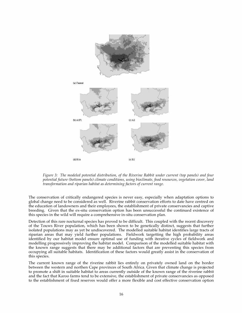
16

Figure 3: The modeled potential distribution, of the Riverine Rabbit under current (top panels) and four potential future (bottom panels) climate conditions, using bioclimate, food resources, vegetation cover, land transformation and riparian habitat as determining factors of current range.

The conservation of critically endangered species is never easy, especially when adaptation options to global change need to be considered as well. Riverine rabbit conservation efforts to date have centred on the education of landowners and their employees, the establishment of private conservancies and captive breeding. Given that the ex-situ conservation option has been unsuccessful the continued existence of this species in the wild will require a comprehensive in-situ conservation plan. Detection of this rare nocturnal species has proved to be difficult. This coupled with the recent discovery of the Touws River population, which has been shown to be genetically distinct, suggests that further isolated populations may as yet be undiscovered. The modelled suitable habitat identifies large tracts of riparian areas that may yield further populations. Fieldwork targetting the high probability areas identified by our habitat model ensure optimal use of funding with iterative cycles of fieldwork and modelling progressively improving the habitat model. Comparison of the modelled suitable habitat with the known range suggests that there may be additional factors that are preventing this species from occupying all suitable habitats. Identification of these factors would greatly assist in the conservation of this species. The current known range of the riverine rabbit lies entirely on privately owned land on the border between the western and northen Cape provinces of South Africa. Given that climate change is projected to promote a shift in suitable habitat to areas currently outside of the known range of the riverine rabbit and the fact that Karoo farms tend to be extensive, the establishment of private conservancies as opposed to the establishment of fixed reserves would offer a more flexible and cost effective conservation option

17

and should continue to be pursued. Whether this option will be able to afford the levels of protection that this critically endangered species will require for persistence in the wild will need to be assessed, especially as hunting by farm employees and their dogs has been highlighted as a significant threat. With imminent legislation allowing for landowners to be compensated for limiting further development and employing conservation practices high priority areas of suitable habitat for both current and future climate should be identified as soon as possible. The model results from this study would be able to guide conservation authorities in this regard. Semi-arid regions in southern Africa have an under-representation of hydro-meteorological stations and as such care should be taken when interpreting these modelled results as they are based in part on interpolated current climatic surfaces as well as modelled future climate with its concomitant uncertainty. It is also recommended that other GCM’s be investigated as the HADCM3 model is acknowledged as providing a pessimistic view of future climate for the southern African region. Owing to the fact that modelled current and future suitable habitat areas are disjunct a translocation of this species is likely to be needed. Translocation of mammals between conservation areas has a long-standing history in conservation. However, recent concerns about the selection of populations to ensure success, the consequences of introducing novel genetic material and the unintended consequences of introduction, for example, invasion will need to be considered. Continued inter-provincial conservation agency co-operation will be a key factor in the short term survival of the riverine rabbit, especially as a third provincial agency will need to be included in deliberations of adaptation to climate change with the bulk of the future suitable habitat projected to lie in the eastern Cape. Given that the population numbers of this species have dipped alarming in the last decade, the amount of conservation planning that is still needed and the complications that climate change will introduce it is suggested that the cryo-preservation of genetic material be promoted as a safe-guard against the permanent disappearance if this species. Homopus signatus: Padloper tortoise

The results of the three modelling techniques applied to this set of subspecies indicate that the predicted distributions are robust regardless of the technique. AUC values of greater than 0.8 indicate that all models are good and would be suitable to undertake investigations into environmental factors driving Homopus signatus distribution as well as projection of these models to investigate future climate change impacts. Environmental variables

The environmental variables highlighted by the three techniques suggest that seasonal patterns of solar radiation, moisture availability and environmental temperature expressed as either mean temperature or heat units are important environmental factors driving, at least in part, the distribution of Homopus signatus. These variables are not unexpected and are a confirmation of the a priori biological and ecological knowledge that was utilised for variable selection. Of note is the selection of winter solar radiation and summer precipitation in all models and suggests that these variables might be significant drivers of Homopus signatus distribution. In the case of winter solar radiation, it is difficult to assess the significance, as it may be directly, i.e. a function of the energy balance of the herbivorous ectotherm that utilises basking to elevate body temperatures above that of the ambient environment, or indirectly related, i.e. related to the July-September flowering season, to the tortoise distribution. While tortoise activity in autumn and winter has been noted for Homopus signatus cafer further clarity is needed for the northerly sub-species. These periods may well be exploited by Homopus signatus as well. It is likewise difficult to assess the significance of summer precipitation as it too could be directly, i.e. summer activity of tortoises following rainfall in search of water to re-establish osmotic homeostasis following a spring diet rich in electrolytes, or indirectly, i.e. summer rainfall may affect the quality of the autumn-winter-spring flowering seasons, related to the tortoise distribution. The models that were reformulated without solar radiation as a predictive environmental variable become almost exclusively a function of moisture availability with seasonal precipitation and humidity being dominant variables.

18

Modelled currently suitable habitat

Evaluation of the habitat suitability model calibrated for all species confirms that the models are robust. The predicted suitable habitat (Figure 4) covers the known distribution and in addition predicts suitable areas predominantly within the Western Mountain, Tankwa and Little Karoo’s. It is uncertain if this identifies possible range that has not been surveyed or if it is the result of over-prediction by the model. Incorporation of the resource variable into the model does not significantly improve or weaken the predictive power or the predicted suitable habitat of the model (Figure 4). Comparison of these ranges with the Succulent Karoo biome constructed from a recently compiled vegetation map indicate a large degree of congruence suggesting that despite these tortoises being restricted to, but being well distributed across, the Namaqualand region of the Succulent Karoo the climatic conditions within this sub-biome are sufficiently similar with those of the remainder of the biome. The fact that Namaqualand is separated from the Tankwa and ergo the other portions of the Succulent Karoo by a watershed divide running from Calvinia to Nieuwhoudtville suggests that the realised niche of Homopus signatus signatus may be a function of a biogeographical divide. The range of a related rocky outcrop species, Homopus boulengeri, occupies portions of the Little, Western Mountain and Tankwa Karoo’s at the eastern edge of the predicted range (see Figure 4).

Figure 4: Modelled current ranges of Homopus signatus, Homopus signatus signatus and Homopus signatus cafer excluding (a, b, c, respectively) and including (d, e, f, respectively) the forage resource variable.

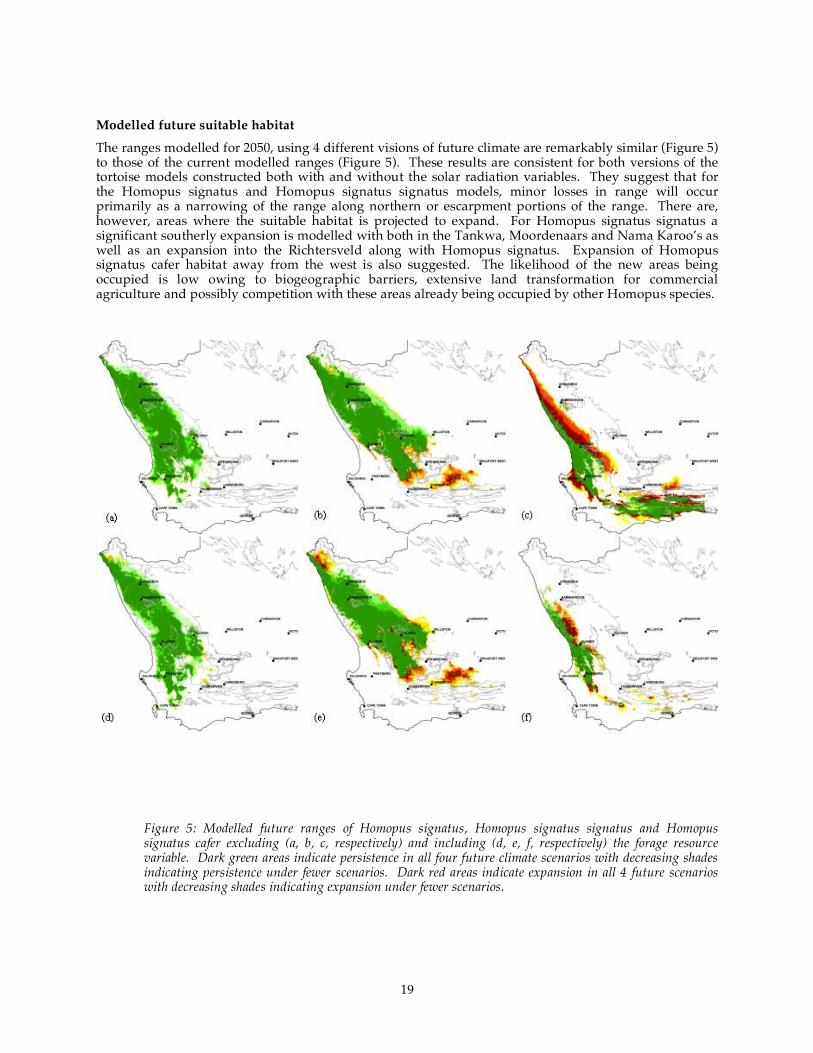
19

Modelled future suitable habitat

The ranges modelled for 2050, using 4 different visions of future climate are remarkably similar (Figure 5) to those of the current modelled ranges (Figure 5). These results are consistent for both versions of the tortoise models constructed both with and without the solar radiation variables. They suggest that for the Homopus signatus and Homopus signatus signatus models, minor losses in range will occur primarily as a narrowing of the range along northern or escarpment portions of the range. There are, however, areas where the suitable habitat is projected to expand. For Homopus signatus signatus a significant southerly expansion is modelled with both in the Tankwa, Moordenaars and Nama Karoo’s as well as an expansion into the Richtersveld along with Homopus signatus. Expansion of Homopus signatus cafer habitat away from the west is also suggested. The likelihood of the new areas being occupied is low owing to biogeographic barriers, extensive land transformation for commercial agriculture and possibly competition with these areas already being occupied by other Homopus species.

Figure 5: Modelled future ranges of Homopus signatus, Homopus signatus signatus and Homopus signatus cafer excluding (a, b, c, respectively) and including (d, e, f, respectively) the forage resource variable. Dark green areas indicate persistence in all four future climate scenarios with decreasing shades indicating persistence under fewer scenarios. Dark red areas indicate expansion in all 4 future scenarios with decreasing shades indicating expansion under fewer scenarios.

20

4.3.3 Savanna case study: Modelling future primary production, habitat, and carrying capacity in African savanna ecosystems

4.3.3.1 Introduction

The natural vegetation cover over about two-thirds of Sub-Saharan Africa is savanna, and the majority of the area in Africa that is primarily managed for biodiversity conservation and nature-based tourism falls in savannas. Thus the capability to predict changes in habitat conditions and wildlife stocking rate and species mix in savannas, under 21st century scenarios of climate and atmospheric change, is important both for the managers of those areas and for the tourism sector which they support. This section outlines a relatively simple procedure, based on empirical equations, for predicting the key functional properties of savannas (tree cover, fire frequency, grass and browse production and carrying capacity for major guilds of herbivores and carnivores). The equations are generally ‘reduced forms’ ie simplified versions of more complex underlying mechanistic models. They are valid for modest changes in rainfall (+15%), temperature (up to 5°C above the 1960-1990 climate normal) and atmospheric carbon dioxide concentration (up to 700 ppm). The ‘ecosystem function’ approach described here is complementary to species-based climate niche modelling. Niche modelling tells you if a species is likely to exist in a given location in the future, whereas ecosystem function models tell you how it is likely to perform. This section attempts to seamlessly hybridise the two approaches. Once the capacity to support a given guild has been calculated, the species composition within that guild is calculated from the niche requirements of individual representative species. The input data and computational requirements have been deliberately kept very simple: the equations can be executed in a spreadsheet, with minimal modelling training and no specialist software. The equations apply to a single, homogeneous location whose spatial extent is not defined, but would conceptually be between 1 and 10000 km2. If a representation of spatial heterogeneity within the study area is considered necessary (for instance, if it spans a major soil or climate contrast), the equations can be solved for a number of different combinations of climate and soil type, and then weighted by the fraction of the total area represented by that combination. If it is desired to simulate a higher degree of spatial heterogeneity (tens to hundreds of unique combinations, rather than two to ten), then it is probably be more efficient to code the equations into a raster-based geographic information system (GIS). Note that the apparent precision gained by such an approach is almost certainly greater than the uncertainty in the equations, which is overall about 25%. It would therefore only be justified if you need to solve an explicitly spatial question, such as species migration. The climate inputs are designed to be directly extractable from the IPCC data directory. All that is required is, summertime (DJF) and wintertime (JJA) mean maximum and minimum temperature and rainfall anomalies (the difference between their future and ‘normal’ values1) at one or more given times in the future. An appropriate time horizon for practical nature conservation management and for the modelling approach outlined here is fifty to one hundred years. Changes over the one to two decade timeframe are likely to be so small as to be lost in the interannual variability. Values for CO2 concentration in the atmosphere at the future times is also needed, and can be estimated from the IPCC Special Report on Emission Scenarios (Nakicenovic et al 2000). For a given emission scenario, the CO2 concentration is approximately the same all over the world, and does not vary appreciably (for this purpose) month-to-month. The CO2, temperatures and rainfall are linearly interpolated for the years

1 Note that temperature and rainfall anomalies are typically averaged over a period of at least a decade, and expressed as the absolute deviation from the climate model calculation of the mean in the 1960-1990 period. This works well for temperature, since the modeled 1960-1990 temperature is quite close to the observed, but can lead to negative rainfall predictions! The rainfall representation in the models is much less accurate. It is better to express rainfall anomalies as relative to the modeled 1960-90 rainfall, ie Ryear –RGCMnormal/RGCMnormal, but the readily accessible data are seldom expressed this way.

21

between each period for which GCM data have been extracted. For each simulated location, you will also need to have the latitude, longitude and altitude of the site, the sand content of the soil, initial values for the tree basal area and stocking rate of various mammals, as well as the mean monthly values for maximum and minimum temperature and rainfall under the current climate. Procedure

The ‘conceptual model’ on which this approach is based is represented in Figure 6.

Figure 6: The components and interactions in a generalised savanna system. The ‘bowties’ are key control points. Each linking arrow is represented by an equation.

Abbrevitions

Subscript indices

normal average for the climate normal period, usually 1960-1990

month month of the year

year year AD

final last year in simulation period

Variables

A basal area of woody plants (m2/ha) B biomass (gDM/m2 for plants, LSU/km2 for mammals, kg LM/km2 for others) C constant in an equation [CO2] annual average atmospheric carbon dioxide concentration (ppm)

Temperature

CO2

Rainfall

Sand %

Tree cover

Sour grass

Tree prodnMixed

Browsers

Coarse graz

Fine grazers

Insects

Small herbiv

Reptiles

Granivore

Insectivore

Raptor

Carnivore

Fire freq

Sweet grass

Frugivore

Temperature

CO2

Rainfall

Sand %

Tree cover

Sour grass

Tree prodnMixed

Browsers

Coarse graz

Fine grazers

Insects

Small herbiv

Reptiles

Granivore

Insectivore

Raptor

Carnivore

Fire freq

Sweet grass

Frugivore

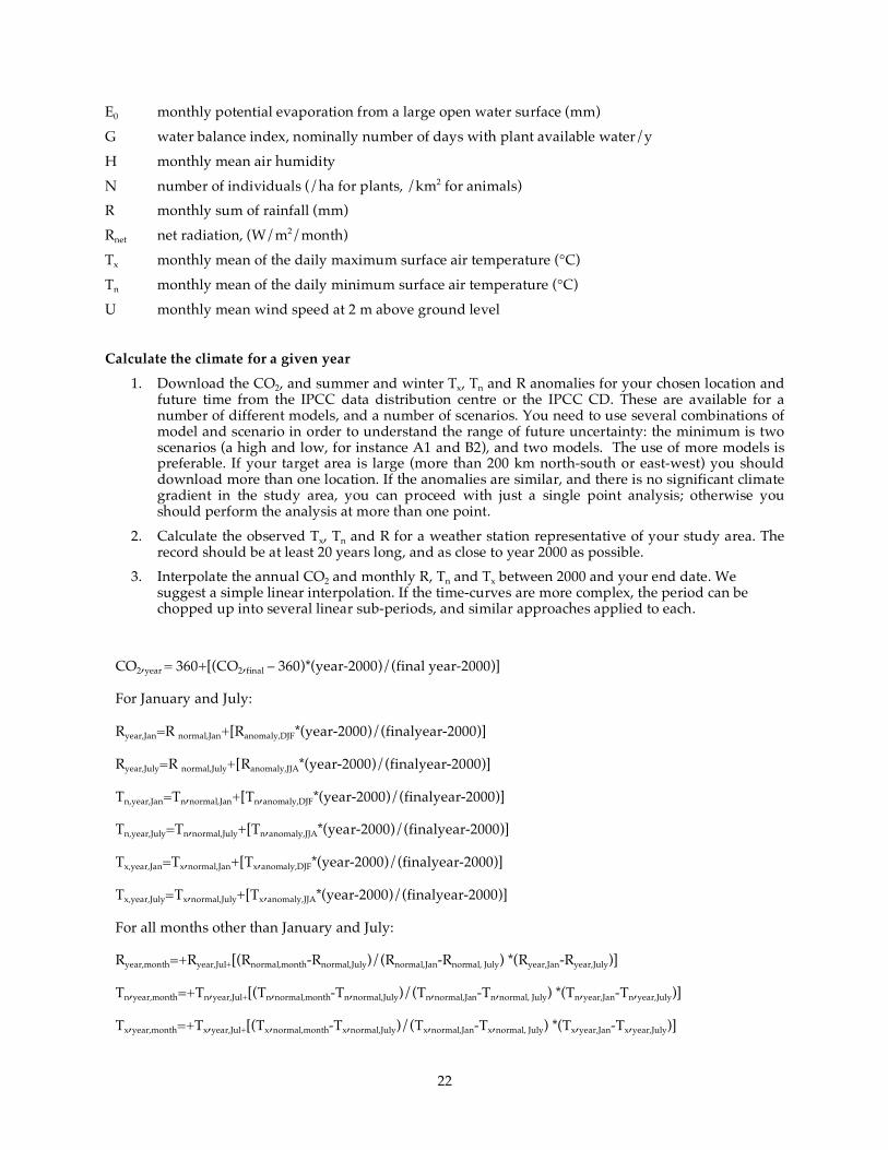
22

E0 monthly potential evaporation from a large open water surface (mm) G water balance index, nominally number of days with plant available water/y

H monthly mean air humidity N number of individuals (/ha for plants, /km2 for animals) R monthly sum of rainfall (mm) Rnet net radiation, (W/m2/month) Tx monthly mean of the daily maximum surface air temperature (°C) Tn monthly mean of the daily minimum surface air temperature (°C) U monthly mean wind speed at 2 m above ground level

Calculate the climate for a given year

1. Download the CO2, and summer and winter Tx, Tn and R anomalies for your chosen location and future time from the IPCC data distribution centre or the IPCC CD. These are available for a number of different models, and a number of scenarios. You need to use several combinations of model and scenario in order to understand the range of future uncertainty: the minimum is two scenarios (a high and low, for instance A1 and B2), and two models. The use of more models is preferable. If your target area is large (more than 200 km north-south or east-west) you should download more than one location. If the anomalies are similar, and there is no significant climate gradient in the study area, you can proceed with just a single point analysis; otherwise you should perform the analysis at more than one point.

2. Calculate the observed Tx, Tn and R for a weather station representative of your study area. The record should be at least 20 years long, and as close to year 2000 as possible.

3. Interpolate the annual CO2 and monthly R, Tn and Tx between 2000 and your end date. We suggest a simple linear interpolation. If the time-curves are more complex, the period can be chopped up into several linear sub-periods, and similar approaches applied to each.

CO2,year = 360+[(CO2,final – 360)*(year-2000)/(final year-2000)]

For January and July:

Ryear,Jan=R normal,Jan+[Ranomaly,DJF*(year-2000)/(finalyear-2000)]

Ryear,July=R normal,July+[Ranomaly,JJA*(year-2000)/(finalyear-2000)]

Tn,year,Jan=Tn,normal,Jan+[Tn,anomaly,DJF*(year-2000)/(finalyear-2000)]

Tn,year,July=Tn,normal,July+[Tn,anomaly,JJA*(year-2000)/(finalyear-2000)]

Tx,year,Jan=Tx,normal,Jan+[Tx,anomaly,DJF*(year-2000)/(finalyear-2000)]

Tx,year,July=Tx,normal,July+[Tx,anomaly,JJA*(year-2000)/(finalyear-2000)]

For all months other than January and July:

Ryear,month=+Ryear,Jul+[(Rnormal,month-Rnormal,July)/(Rnormal,Jan-Rnormal, July) *(Ryear,Jan-Ryear,July)]

Tn,year,month=+Tn,year,Jul+[(Tn,normal,month-Tn,normal,July)/(Tn,normal,Jan-Tn,normal, July) *(Tn,year,Jan-Tn,year,July)]

Tx,year,month=+Tx,year,Jul+[(Tx,normal,month-Tx,normal,July)/(Tx,normal,Jan-Tx,normal, July) *(Tx,year,Jan-Tx,year,July)]

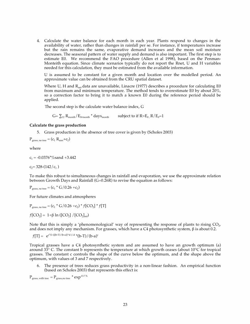
23

4. Calculate the water balance for each month in each year. Plants respond to changes in the availability of water, rather than changes in rainfall per se. For instance, if temperatures increase but the rain remains the same, evaporative demand increases and the mean soil moisture decreases. The seasonal pattern of water supply and demand is also important. The first step is to estimate E0. We recommend the FAO procedure (Allen et al 1998), based on the Penman-Monteith equation. Since climate scenarios typically do not report the Rnet, U and H variables needed for this calculation, they must be estimated from the available information. U is assumed to be constant for a given month and location over the modelled period. An approximate value can be obtained from the CRU spatial dataset. Where U, H and Rnet data are unavailable, Linacre (1977) describes a procedure for calculating E0 from maximum and minimum temperature. The method tends to overestimate E0 by about 20%, so a correction factor to bring it to match a known E0 during the reference period should be applied. The second step is the calculate water balance index, G

G= ∑12 Rmonth/E0,month * daysmonth subject to if R>E0 , R/E0=1

Calculate the grass production

5. Grass production in the absence of tree cover is given by (Scholes 2003) Pgrass, no tree = (c1 Rann+c2)

where

c1 = -0.0376*%sand +3.442

c2= 328-(142/c1 )

To make this robust to simultaneous changes in rainfall and evaporation, we use the approximate relation between Growth Days and Rainfall (G=0.26R) to revise the equation as follows: Pgrass, no tree = (c1 * G/0.26 +c2)

For future climates and atmospheres

Pgrass, no tree = (c1 * G/0.26 +c2) * ƒ[CO2] * ƒ[T]

ƒ[CO2] = 1+β ln ([CO2] /[CO2]ref)

Note that this is simply a ‘phenomenological’ way of representing the response of plants to rising CO2, and does not imply any mechanism. For grasses, which have a C4 photosynthetic system, β is about 0.2.

ƒ[T] = ec*(1-{[(b-T)/(b-a)]^d }/d *(b-T)/(b-a)c

Tropical grasses have a C4 photosynthetic system and are assumed to have an growth optimum (a) around 33° C. The constant b represents the temperature at which growth ceases (about 10°C for tropical grasses. The constant c controls the shape of the curve below the optimum, and d the shape above the optimum, with values of 3 and 7 respectively.

6. The presence of trees reduces grass productivity in a non-linear fashion. An empirical function (based on Scholes 2003) that represents this effect is:

Pgrass, with tree = Pgrass,no tree * exp-0.1*A

24

Calculate the tree production

7. The annual growth in tree basal area is given by the following equation (Scholes and Shackleton, in prep)

ΔA = [1.12*(1-exp-x*d) * (1-A/Amax)] * ƒ[CO2] * ƒ[T]

where

Amax = f*G+i

D= A/ntrees

ƒ[CO2] = 1+β ln ([CO2] /[CO2]ref)

For trees, which have a C3 photosynthetic system, β is about 0.4.

ƒ[T] = ec*(1-{[(b-T)/(b-a)]^d }/d *(b-T)/(b-a)c

Trees have a C3 photosynthetic system and are assumed to have an growth optimum (a) around 28° C. The constant b represents the temperature at which growth ceases (about 5°C for tropical trees. The constant c controls the shape of the curve below the optimum, and d the shape above the optimum, with values of 3 and 7 respectively.

8. The production of tree leaf is given by

Pbrowse = ntrees * m*d2

Where m is 0.01 kg/cm2.

Calculate the biomass per animal guild

9. The same basic equations (conceptually based on Lotka-Volterra predator-prey equations and logistic growth curves) are used for simulating the population sizes of all mammal guilds. Note that ‘predator’ just means the guild at a higher tropic level: grazers are predators on grass.

Bpredator, t+1 = Bpredator t * r

r = r predator,max (B predator,t * a/ Bprey)

where rmax is the intrinsic growth rate of the species (itself typically a function of mean body mass) and a is a factor including both the wastefulness of consumption of the prey and the degree to which finding prey becomes more difficult as it becomes scarcer. The tropic web defined above for savannas is relatively complicated, and it is hard to keep all the guilds in the system at the same time. Mathematical ecology theory teaches that competitors can only exist under certain conditions. Firstly, if they use slightly different resources, and are therefore not in full competition. For this reason a ‘palatable grass’ and an ‘unpalatable grass’ resource are defined, whose proportions depend on the soil sand content. The coarse grazers preferentially use the unpalatable grass, and the fine grazers the palatable grass. Secondly, where more than one prey guild is consumed by one predator guild, the system will only be stable if the better competitor between the prey species is also the more preferred prey by the predator. This notion is included in the model by making predator preference an increasing function of prey biomass proportion. Note that elephants have no top predator, and tend to increase to high biomass densities before food limitation sets in. An elephant ‘predator’, in the form of a removal rule, can be imposed.

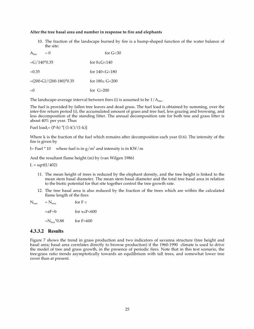
25

Alter the tree basal area and number in response to fire and elephants

10. The fraction of the landscape burned by fire is a hump-shaped function of the water balance of the site:

Afire = 0 for G<30

=G/140*0.35 for 0≤G<140

=0.35 for 140<G<180

=(200-G)/(200-180)*0.35 for 180≤ G<200

=0 for G>200

The landscape-average interval between fires (i) is assumed to be 1/Afire. The fuel is provided by fallen tree leaves and dead grass. The fuel load is obtained by summing, over the inter-fire return period (i), the accumulated amount of grass and tree fuel, less grazing and browsing, and less decomposition of the standing litter. The annual decomposition rate for both tree and grass litter is about 40% per year. Thus Fuel loadi= (P-h) *[ (1-ki)/(1-k)]

Where k is the fraction of the fuel which remains after decomposition each year (0.6). The intensity of the fire is given by I= Fuel * 10 where fuel is in g/m2 and intensity is in KW/m

And the resultant flame height (m) by (van Wilgen 1986) L = sqrt(I/402)

11. The mean height of trees is reduced by the elephant density, and the tree height is linked to the mean stem basal diameter. The mean stem basal diameter and the total tree basal area in relation to the biotic potential for that site together control the tree growth rate.

12. The tree basal area is also reduced by the fraction of the trees which are within the calculated flame length of the fires

Ntree = Ntree for F <

=aF+b for x≤F<600

=Ntree*0.88 for F>600

4.3.3.2 Results

Figure 7 shows the trend in grass production and two indicators of savanna structure (tree height and basal area; basal area correlates directly to browse production) if the 1960-1990 climate is used to drive the model of tree and grass growth, in the presence of periodic fires. Note that in this test scenario, the tree:grass ratio trends asymptotically towards an equilibrium with tall trees, and somewhat lower tree cover than at present.

26

Figure 7: Tree and grass trends, in the presence of fire, under a continuation of the current climate.

When medium-sized mammalian herbivores are added to the ecosystem (both grazers and browsers, but excluding system-altering ‘megaherbivores’, such as elephants), the grazer biomass rises steadily through the simulation period, tracking the increase in grass production, while the browsers initially increase, and then begin to fall as the tree basal area declines (fig 8).

Figure 8: Grazer and browser biomass trends under the current climate, but in the absence of carnivores or elephants.

0

10

20

30

40

50

60

2000 2020 2040 2060 2080 2100

Year

Pla

nts

(m

2/h

a),

(g/m

2),

(m)

Basal Area

Grass prod

Tree ht

0

1 Year

500

1000

1500

2000

2500

3000

2000 2020 2040 2060 2080 2100

Her

bivo

res

(kg/

km2)

Elephants

Coarse

Fine

Browser

Mixed

27

When carnivores (lions, leopards, cheetah and hyenas) are added to the system (Figure 9), their numbers oscillate initially, and then equilibrate with the prey food supply.

Figure 9: Carnivore response under continued normal climate.

Figure 10: Plant response where elephants are included.

When elephants are introduced to the ecosystem, the vegetation structure (Fig 10) and the herbivore guild composition change completely. Elephant biomass rises to four times the current density, showing signs of equilibration with a transformed vegetation towards the end of the century. The trees become short (coppiced) forms, with a basal area about half the current basal area. Grass biomass increased, and then equilibrated with the new basal area. Even so, the grass and browse consumption by the elephants drove the other herbivores to extinction (Fig 11), given that they were subject to carnivore pressure, while elephants are not.

0

5

10

15

20

25

2000 2020 2040 2060 2080 2100

Year

Ca

rniv

ore

s (

kg

/km

2)

0

10

20

30

40

50

60

2000 2020 2040 2060 2080 2100

Year

Pla

nts

(m

2/h

a),

(g/m

2),

(m)

Basal Area

Grass prod

Tree ht

28

Figure 11: Elephant and medium-sized herbivore trends under the current climate.

This completes the ‘reasonability test’ of the model, when run under current climate. All the modelled behaviours are consistent with what is known regarding ecosystem dynamics in the study area. The model is now ready to be explored using climate change scenarios. Figures 12 and 13 show the changes in the drivers of tree and grass production under a high and low scenario of climate change. Note that in both scenarios, the positive effect of elevated CO2 on plant growth is cancelled out or overwhelmed by the negative effects of rising temperature and falling soil water availability. These latter effects are stronger for trees than for grasses, and the result is that unlike the simulations under ‘normal’ climate, where the grasses increased at the expense of the trees, the reverse occurred under climate change (fig 14). This goes contrary to the ‘received wisdom’ that elevated CO2 has a stronger effect on trees than grasses, and therefore trees will tend to take over, and is a new finding that needs more rigorous exploration. The patterns were qualitatively the same for both climate scenarios, suggesting that adaptation is now imperative, since strenuous mitigation efforts will only delay the outcome somewhat.

0

1000

2000

3000

4000

5000

2000 2020 2040 2060 2080 2100

Year

He

rbiv

ore

s (

kg

/km

2)

Elephants

Coarse

Fine

Browser

Mixed

29

Figure 12: Changes in production drivers given a B2 ( 550 ppm CO2 by 2080) scenario of climate change.

Figure 13: Changes in production drivers given a A2 (700 ppm CO2 by 2080) scenario of climate change.

0.0

0.5

1.0

1.5

2.0

2000 2020 2040 2060 2080 2100

Year

Pro

du

cti

on

driv

ers

Water balance

f(CO2)g

f(CO2)t

f(T)g

f(T)t

0.0

0.5

1.0

1.5

2.0

2000 2020 2040 2060 2080 2100

Year

Pro

du

cti

on

driv

ers

Water balance

f(CO2)g

f(CO2)t

f(T)g

f(T)t

30

Figure 14: Changes in vegetation structure given a B2 (Low) scenario of climate change.

Figure 15: Changes in vegetation structure given a A2 (High) scenario of climate change.

0 10

20

30

40

50

60

2000 2020 2040 2060 2080 2100

Year

Plan

ts

(m2/

ha),(

g/m

2),(m

) Basal Area

Grass prod

Tree ht

0

10

20

30

40

50

2000 2020 2040 2060 2080 2100

Year

Pla

nts

(m

2/h

a),

(g/m

2),

(m)

Basal Area

Grass prod

Tree ht

31

When browsers and grazers are added, the patterns are similar to those shown in the ‘normal’ climate scenario, but exaggerated. Under the high rate of climate change scenario, grazer biomass begins to fall after mid-century, due to the declining grass production (figs 16 and 17). Adding elephants again led to profound structural changes.

Figure 16: Changes in herbivore density given a B2 (low) scenario of climate change.

Figure 17: Changes in herbivore density given a A2 (high impact 700 ppm CO2) scenario of climate change.

0

500

1000

1500

2000

2500

3000

2000 2020 2040 2060 2080 2100

Year

He

rbiv

ore

s (

kg

/km

2)

Elephants

Coarse

Fine

Browser

Mixed

0

500

1000 1500

2000

2500

2000 2020 2040 2060 2080 2100

Year

Her

bivo

res

(kg/

km2)

Elephants Coarse Fine Browser Mixed

32

4.3.3.3 Preliminary conclusions of savanna case study

• Water availability and temperature consequences of climate change may overwhelm the elevated CO2 effect on both overall plant production, and vegetation structure.

• Substantial (>20%) decreases in herbivore stocking rate are possible by mid-century as a result of climate change.

• Elephants at high density put the tree cover into a stable coppice state, and this has profoundly negative consequences for the populations of medium-sized browsers and grazers, and therefore carnivores. This effect overshadows the climate change effect, and is partly mediated by fire.

• Therefore, the outcome of climate-change induced habitat change depends on how you manage fires and elephants.

4.4 Human dependencies on biodiversity from the selected biomes

Biodiversity has an intrinsic value, but also a direct and indirect human benefit value. It currently contributes to human livelihoods in the succulent karoo, Fynbos and savanna, and to human well-being of people who live outside these areas, but who, for instance visit them as tourists, or use medicinal or horticultural products derived from them. The value of biodiversity to human well-being is poorly researched. An initial attempt is made to predict some impacts on predicted biodiversity change on livelihoods based on current biodiversity use patterns and the resultant changes in biodiversity based livelihoods per biome. Succulent karoo

This near-desert area has low plant production potential and a very low population density. It has historically been used prominently for livestock grazing, though even with borehole suplied water it is still an inhospitable environment. Stocking rates have decreased over the last two decades and this is attributed to species changes in response to herbivory leading to low palatability of usable production (Dean and McDoanals 1994, Milton et al 1997). It can be assumed that with increasing aridity as predicted by most climate models, that this area will become less suited to livestock production. Changes in the global economics of livestock production are likely to exacerbate this impact. A growing use of the area has been the tourism industry based on the annual wild flower blooms. These are annuals, mostly if the families Asteraceae, Liliaceae and Mesembryanthemaceae. The extent of these blooms is related to seasonal rainfall. A decline in rainfall may therefore directly impact on this industry, as will a shift to more summer rainfall. Fynbos

The Fynbos is an area of high human population, especially on the plains, though the mountains have relatively low population density as they are declared water catchment areas and therefore de facto biodiversity protection areas. Transformation of the area into agricultural and settlement areas has had strong impacts on biodiversity, but natural biodiversity per se is not the basis of the main economic activity in the biome. Individual species of the Fynbos are extensively used for the cut flower and dry flower industry, for flavouring brandy (buchu) and for herbal tea (rooibos tea). The vegetation is also used for fuelwood, though much of this is from alien invasive species. Changes in availability and location of the commercialisable species will impact directly on these industries. In addition, the Fynbos is a major tourist attraction, though how closely tourism can be linked to actual species biodiversity is unclear. It is unlikely to be a linear relationship. Loss of biodiversity is unlikely to be measured in direct loss of tourism. The role of Fynbos clad catchments for water supply in this area is critical. Invasion of alien vegetation has a high negative impact on water yield, and this has been a long standing political driver for biodiversity conservation. Climate change could accelerate the rate of alien invasion. Savanna biome

The savanna biome is used predominantly for livestock grazing or wildlife management, including nature-based tourism. There is a growing literature on the importance of the savannas for the provision of

33

livelihood benefits to improvised rural communities (e.g. Campbell 1992, Shackleton et al, 1994). Within South Africa most of the communally-managed areas occur in the savannas, and these have extensive rural communities who derive large proportions of their livelihoods from the natural biodiversity of the savanna. This trend is even more prevalent in other southern African countries where there is less of a cash economy and a poorer state social support network. By far the most important resource from the savannas to these subsistence communities is fuel wood and grazing, though many other resources including construction timber, edible plants, medicinal plants and craft material are also collected. Although species may change as a consequence of climate change, it is likely that the range of services derived from savannas will still be maintained (though possibly at a somewhat lower level). Because the climate of these areas may become less hospitable to crop production the reliance on natural products may increase. The potential of the savannas to support a wildlife based tourism industry is also not envisaged as collapsing as a consequence of climate change. The same is probably true of the livestock industry, though climate change may accelerate the current change that is being observes from livestock to wildlife management. This is predicted due to the greater resilience of wildlife in a hot and dry environment and the possibility of increased problems for cattle from pathogens.

4.5 Conclusions During the conceptualization phase of this project, simple niche-based ecosystem-level habitat models were considered as the methods to use. Rapid advances in individual species modelling approaches allowed us to rather develop detailed approaches based on individual species responses. These approaches let us better understand conservation options based on the actual migratory corridors of individual species. Our objective was not to develop definitive solutions for biodiversity conservation, but rather to explore a range of tools and techniques as a way of better understanding options for more detailed research. In this regard we were able to develop and test very complex models for individual species predictions. These powerful models should be considered as techniques where impacts are already predicted. We would recommend that far simpler envelope-based screening techniques should be applied to an area first to confirm that there are likely to be major biodiversity impacts, before detailed individual species approaches are considered. The savanna case study takes a very different approach to understanding climatic impacts. Rather than considering individual species, it concentrates on functional ecosystem level attributes of the area given climate change. These two approaches should be seen as complimentary rather than competing.

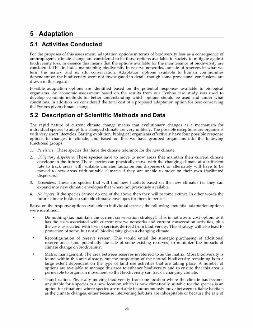
34

5 Adaptation 5.1 Activities Conducted For the proposes of this assessment, adaptation options in terms of biodiversity loss as a consequence of anthropogenic climate change are considered to be those options available to society to mitigate against biodiversity loss. In essence this means that the options available for the maintenance of biodiversity are considered. This includes maintaining biodiversity in reserve networks, outside of reserves in what we term the matrix, and ex situ conservation. Adaptation options available to human communities dependant on the biodiversity were not investigated in detail, though some provisional conclusions are drawn in this regard. Possible adaptation options are identified based on the potential responses available to biological organisms. An economic assessment based on the results from our Fynbos case study was used to develop economic methods for better understanding which options should be used and under what conditions. In addition we considered the total cost of a proposed adaptation option for best conserving the Fynbos given climate change.

5.2 Description of Scientific Methods and Data The rapid nature of current climate change means that evolutionary changes as a mechanism for individual species to adapt to a changed climate are very unlikely. The possible exceptions are organisms with very short lifecycles. Barring evolution, biological organisms effectively have four possible response options to changes in climate, and based on this we have grouped organisms into the following functional groups: 1. Persisters. These species that have the climate tolerance for the new climate. 2. Obligatory dispersers. These species have to move to now areas that maintain their current climate

envelope in the future. These species can physically move with the changing climate at a sufficient rate to track areas with suitable climates (autonomous dispersers), or alternately will have to be moved to new areas with suitable climates if they are unable to move on their own (facilitated dispersers).

3. Expanders. These are species that will find new habitats based on the new climates i.e. they can expand into new climatic envelopes that where not previously available.

4. No hopers. If the species cannot do one of the above then they will become extinct. In other words the future climate holds no suitable climatic envelopes for them to persist.

Based on the response options available to individual species, the following potential adaptation options were identified:

• Do nothing (i.e. maintain the current conservation strategy). This is not a zero cost option, as it has the costs associated with current reserve networks and current conservation activities, plus the costs associated with loss of services derived from biodiversity. This strategy will also lead to protection of some, but not all biodiversity given a changing climate.

• Reconfiguration of reserve system. This would entail the strategic purchasing of additional reserve areas (and potentially the sale of some existing reserves) to minimize the impacts of climate change on biodiversity.

• Matrix management. The area between reserves is referred to as the matrix. Most biodiversity is found within this area already, but the proportion of the natural biodiversity remaining is to a large extent dependant on the type of land use activities that are taking place. A number of options are available to manage this area to enhance biodiversity and to ensure that this area is permeable to organism movement so that biodiversity can track a changing climate.

• Translocation. Physically moving biodiversity from one location where the climate has become unsuitable for a species to a new location which is now climatically suitable for the species is an option for situations where species are not able to autonomously move between suitable habitats as the climate changes, either because intervening habitats are inhospitable or because the rate of

35

migration is too slow, or the distance too long. This is currently a common practice for large animals but is seldom used for plants and insects.

• Ex-situ conservation. If the future holds no suitable habitats for a species to persist naturally then the only mechanism left to prevent extinction will be ex-situ conservation. This could be in zoos, botanical gardens, seedbanks or by means of cryo-preservation.

An economic analysis was undertaken on the costs of different conservation option. The Fynbos case study (Williams et al 2004 and as presented above) was used as the basis for the analysis. The Western Cape was an ideal test site because of the extensive data that has already been collected during the GEF funded Cape Action Programme for the Environment. In determining the economic costs of adaptation options we made the up-front assumption that benefits should be measured as the number of species that would be conserved using different adaptation strategies. This decision was made instead of attempting to derive a total economic value of saved species. Total economic valuation was discarded because a) there was no objective way to value non-use values, b) many non-consumptive use values cannot be objectively distributed between different biota in any specific habitat and c) we did not want to find solutions based purely on current human values.

5.3 Results Clearly, where a species persists under future climates in large populations in already-conserved areas, there is no basis for concern. If the global population inside and outside of protected areas under future climates is too small to be viable, then there is a need for ex situ conservation actions, even though the protected areas may still fall within the climate niche of the species. Where a species needs to move to a new habitat outside of its current range, or where the future habitats are all outside protected areas, or where the future holds no suitable habitats, then human intervention is likely to be needed to ensure that the species does not become extinct. There are a number of adaptation options available to help minimise the species loss as a consequence of climate change. For obligatory dispersers there are basically two scenarios, one where the species can reach a new habitat through natural dispersal mechanisms, at a rate sufficient to keep up with the shifting climate; and the other where natural dispersal is inadequate for the species to reach a new habitat. In the first instance a climatically and environmentally suitable pathway exists to allow the species to move through the landscape to track the changing climate. We will refer to these as autonomous obligatory dispersers, in comparison to the facilitated obligatory dispersers in the alternative scenario. For autonomous obligatory dispersers, the key question is: Are there suitable migratory pathways that will allow the species to move from its current location to a future protected area? There are two options for protecting migratory pathways. The first is to expand the existing reserve network to protect the migratory pathways. This is often referred to as creating protected corridors. The second is to ensure that the matrix is sufficiently protected to allow the species to travel through the area sufficiently freely to ensure its survival. For facilitated obligatory dispersers the only option to prevent extinction is to physically move the species to the new suitable habitat. Movement of large mammals and birds is a well-established practice in conservation circles, regularly undertaken throughout the sub-region. However, it is usually undertaken to reintroduce species to locations where they are extinct or threatened within what is believed to be their historical range. Introduction of species to places where they probably did not exist within the recorded past is frowned upon. To conservators, pre-emptive facilitated movement, especially of plants and insects, is a new concept. Facilitated dispersal will have ethical and practical considerations such as:

• What size population needs to be moved to re-establish a new viable population? • Under what circumstances should a species be moved to an area where it did not historically

exist, and what impact will this have on the species currently occurring in that area?

• Which species need to be moved together, in order to preserve the community structure? • How is the pattern of genetic variability within the population to be maintained?

36

For the no-hopers the only non-fatalistic option is to maintain the biodiversity in artificial situations such as zoos, botanical gardens, seed banks and through cryo-preservation. Some autonomous dispersers, and some facilitated dispersers, are likely to become ‘weeds’, ie overabundant in their new habitats, to the detriment of other species. The most likely candidates are primary succession species that are well adapted to dispersal into new habitats. Weed outbreaks, including from alien species from other continents, will be further encouraged by the disruption of communities in the receiving environment, directly or indirectly due to climate change, and by the possibility that the invasive species will travel faster than their natural competitors and controlling agents. Range expansion is a potential threat to the species currently established in the new areas. A further concern is that climate change may well favour introduced exotic species which may become invasive. Control of invasive species may be needed to protect the vegetation indigenous to an area and to provide opportunity for less aggressive species to establish in new areas. The optimal adaptation strategy differs for different species dependant on the level of threat placed on them by climate change, and on the ability of the species to move to new, suitable habitats. Figure 18 gives and overview of the adaptation strategies to be considered for different species.

Surrogate

species

Range

expanders

No hopers

Persisters

Obligatory

dispersers

Endemic alien

potential

Limited invasion

potential

Alien control

No response

Ex-Situ

conservation

Minimal range

reduction

IUCN Red Data

range reduction

No response

Existing PA's

Adjunct to

existing PA's

Matrix

management

Autonomouse

dispersers

Facilitated

dispersers

Expand

existing PA's

Matrix

management

New PA's

Ex-Situ

conservation

Assisted

migration/

translocation

Existing

reserves

New reserves

Matrix

Disjunct to

existing PA's

Figure 18: A decision tree for selecting adaptation strategies for different surrogate species based on their response to climate change (Adapted from Midgley et al in prep).

37

Economic considerations relating to adaptation options

The Fynbos biome, and particularly the conservation of members of the Proteaceae, was used as a case study to investigate the costs and benefit of the various adaptation options discussed above. (Letsoalo et al in prep). A modelling process was used to identify the areas critical for conserving migratory pathways, as well as identifying disjunct habitats and no-hoper species (see the fynebos case study above and Williams et al 2004). Land acquisition cost

The costs of land acquisition vary according to different habitat types and Table 2 shows once-off costs of acquiring different habitat types in the Cape Floristic Region. Land prices are to a large extend related to the economic potential of the land. The cost of acquiring land in dry mountain Fynbos and karoo is relatively low, but these areas have limited production potential other than for extensive grazing of livestock. . Lowland Fynbos is extensively transformed for crop production of which winter wheat is the most common crop, especially in the dryer areas. Costal Fynbos is the most valuable land. Grapes for wine making are an important intensive land use.

Source: Frazee, et al. (2003)

a Land not transformed by agriculture, urbanisation and dense stands of invasive alien plants.

Table 2: Once-off costs of acquiring different habitat types in the Cape Floristic Region.

Operating cost and capital requirement costs Per hectare costs decrease rapidly as protected area (PA) size increases (Frazee et al. 2003, Balmford et al. 2003, Vreugdenhil 2003, ART 1998) because larger areas benefit from number of factors. These factors include economies of scale in management, more area that is protected by inaccessibility, and that large protected areas suffer less from edge effects and are more likely to be ecologically self-sustaining (Gascon et al. 2000, Nepstad et al. 1999). Thus, small-protected areas usually cost more to manage per unit area than larger ones, owing to management complexity and economies of scale (Shafer, 1990; Howard and Young, 1995; Press et al. 1996; Bowers, 1997; Young and Gunningham, 1997; Hoctor et al. 2000). From a literature review conducted and specifically a study undertaken in the Cape Floristic Region (CFR) by Frazee et al. (2003), it was established that size was the most important predictor of management costs of protected areas in the CFR. There are strong relationships between total required expenditure per ha and some of the physical and biological attributes of protected areas. Table 3 shows that management requirement vary with habitat classes. Management requirement include amongst others control of invasive alien species and fire

Cost of all remaining extant habitat in the Cape Floristic Region (CFR)a

Hectare Value of Cost (US$) Cost (US$)

per hectare

Coastal 214421 183020916 853.6

Lowland 1660142 634509691 382.2

Dry mountain Fynbos 897859 23942899 26.7

Wet mountain Fynbos 1230471 55348180 45.0

Karoo 1053936 28104955 26.7

Forest and thicket 153465 130905645 853

38

management. It is evident that coastal areas have higher management requirements compared to mountain Fynbos and karoo. Lowland and wet mountain Fynbos have medium management requirement.

Habitat class

Primary BHU representeda Management requirements

Control of

invasive alien species

Wildfire control

Prescribed burning

Ecological monitoring requirements

Coastal Dune pioneer, Fynbos/Thicket Mosaic, Strandveld

High High Medium High

Lowland Sand Plain Fynbos, Limestone Fynbos, Grassy Fynboss, Fynbos/Renosterveld Mosaic, Coast Renosterveld, Inland Renosterveld

High Medium Medium Medium

Forest and thicket

Afrom on tane Forest, Indian Ocean Forest, Mesic Succulent Thicket

Medium Low Low High

Wet Mountain Fynbos

Mountain complex Medium Medium Medium Medium

Dry Mountain Fynbos

Inland Renosterveld, Mountain Complex

Low Low Low Low

Karoo Vygieveld, Broken Veld, Xeric Succulent Thicket

Low Low Low Low

Source: Frazee, et al. (2003).

Table 3: Habitat classes and associated management requirements for protected areas in the Cape Floristic Region. Martin (2003) and Frazee, et al. (2003) has shown that increasing conservation area significantly lead to reduction in management costs. This relationship is non-linear: the unit costs of management requirement escalated dramatically at protected area sizes smaller than 10 km2 (see Table 3). Therefore, unless one can incorporate small areas into larger protected areas or the area that is very important for biodiversity conservation purposes, land acquisition of smaller areas is unlikely to be economically and financially viable to buy and hence, should not be considered. Not only are small protected areas expensive to manage relative to larger reserves, they are also not able to support species with extensive habitat requirements (Noss and Cooperrider, 1994; Terborgh et al., 1999; Kerley et al., 2003) and are too small to maintain many ecological and evolutionary processes (Pickett and Thompson, 1978; Balmford et al., 1998). Operational costs in conservation budgets include salaries, field allowances, equipment, transport and maintenance costs and also includes provisions for senior field and research staff (Martin, 2003). These costs exclude the cost of alien species eradication. Martin (2003) used the following formulas to estimate

39

the annual recurrent expenditure/km2 (operating cost) and total capital expenditure/ km2 required for various parks sizes in South Africa.

Annual recurrent expenditure/km2 )

321(50$

AAUSC

R++=

And total capital expenditure/km2 )

111(500$

AAUSC

C++=

Where A is expressed in thousands of square kilometres.

Table 5 and Figure 19 and 20 shows the operating and capital requirement for various park sizes in South Africa. The units used in the table are US dollars per square kilometre and can be easily converted to hectares as outlined below Table 4. The operating costs for an area of 10 km2 is US$115 500 per km2 per year while the capital requirement is US$555 000 per km2. The operating costs for 100 km2 is US$152 434 per km2 per year while the capital requirement is US$708 114 per km2. The operating cost and capital requirement decline as the area under protected area network increases. Table 5 presents management costs using price per hectare as suggested by Frazee, et al. (2003) and James, et al, (1999b) and the figures appear to be much higher than the values derived using method by Martin (2003). This study will adopt a conservative approach and use the values derived using method by Martin (2003). Figures 1 and 2, shows that both operating costs and capital requirement decline as the park size increases because mainly economies of scale and other related factors. Therefore, it becomes relatively cheaper to establish bigger parks than smaller ones.

Source: Martin (2003), compiled for South African National Parks.

Note: 1 km2 = 1 00 hectare (www.metric-conversions.org).

Table 4: Operating and capital costs for various park sizes.

Park size

(KM2)

Number of

staff needed

Operating costs

(US$/KM2/year

Total operating

costs(US$/year)

Capital costs

(US$/KM2)

Total capital costs

US$

1 1 104 793 104 793 516 311 516 311

2 1 53 404 106 808 261 680 523 361

5 2 22 171 110 857 107 571 537 855

10 3 11 550 115 500 55 500 555 000

20 4 6 111 122 213 29 036 580 711

50 7 2 721 136 041 12 736 636 803

62 8 2 271 140 386 10 599 655 228

100 10 1 524 152 434 7 081 708 114

200 14 885 177 082 4 118 823 607

500 22 462 231 066 2 207 1 103 553

1 000 32 300 300 000 1 500 1 500 000

2 000 45 206 412 132 1 104 2 207 107

2 415 49 188 453 812 1 029 2 484 229

2 476 50 186 459 868 1 020 2 525 022

5 000 71 137 685 410 824 4 118 034

10 000 100 107 1 074 342 708 7 081 139

20 000 141 89 1 770 820 637 12 736 068

50 000 224 73 3 660 660 581 29 035 534

100 000 316 66 6 600 000 555 55 500 000

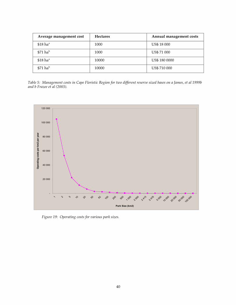
40

Average management cost Hectares Annual management costs

$18 haa 1000 US$ 18 000

$71 hab 1000 US$ 71 000

$18 haa 10000 US$ 180 0000

$71 hab 10000 US$ 710 000

Table 5: Management costs in Cape Floristic Region for two different reserve sized bases on a James, et al 1999b and b Frazee et al (2003).

Figure 19: Operating costs for various park sizes.

-

20 000

40 000

60 000

80 000

100 000

120 000

1

2

5

10

20

50

62

100

200

500

1 0

00

2 0

00

2 4

15

2 4

76

5 0

00

10 0

00

20 0

00

50 0

00

100 0

00

Park Size (km2)

Op

era

tin

g c

os

ts p

er

km

2 p

er

ye

ar

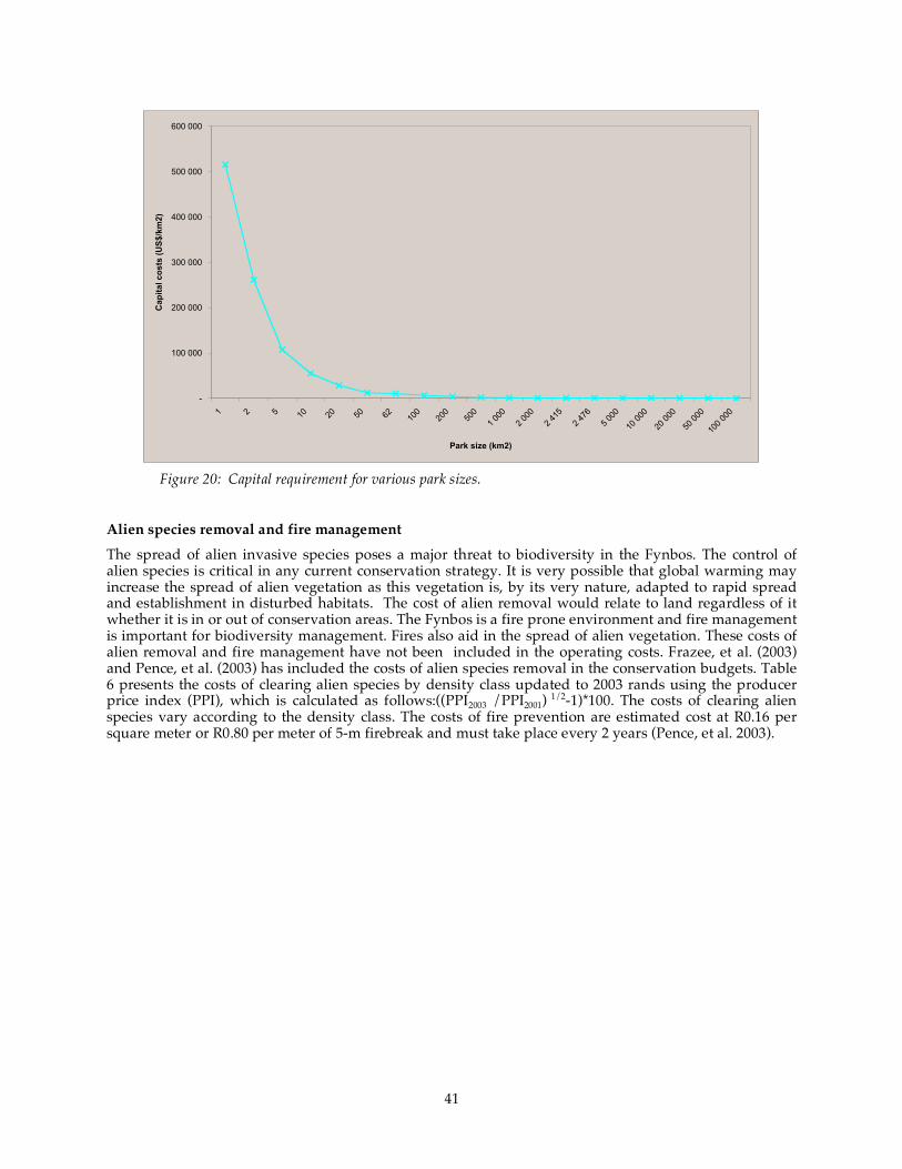
41

Figure 20: Capital requirement for various park sizes.

Alien species removal and fire management

The spread of alien invasive species poses a major threat to biodiversity in the Fynbos. The control of alien species is critical in any current conservation strategy. It is very possible that global warming may increase the spread of alien vegetation as this vegetation is, by its very nature, adapted to rapid spread and establishment in disturbed habitats. The cost of alien removal would relate to land regardless of it whether it is in or out of conservation areas. The Fynbos is a fire prone environment and fire management is important for biodiversity management. Fires also aid in the spread of alien vegetation. These costs of alien removal and fire management have not been included in the operating costs. Frazee, et al. (2003) and Pence, et al. (2003) has included the costs of alien species removal in the conservation budgets. Table 6 presents the costs of clearing alien species by density class updated to 2003 rands using the producer price index (PPI), which is calculated as follows:((PPI2003 /PPI2001) 1/2-1)*100. The costs of clearing alien species vary according to the density class. The costs of fire prevention are estimated cost at R0.16 per square meter or R0.80 per meter of 5-m firebreak and must take place every 2 years (Pence, et al. 2003).

-

100 000

200 000

300 000

400 000

500 000

600 000

1

2

5

10

20

50

62

100

200

500

1 0

00

2 0

00

2 4

15

2 4

76

5 0

00

10 0

00

20 0

00

50 0

00

100 0

00

Park size (km2)

Ca

pit

al

co

sts

(U

S$

/km

2)

42

Density class (% cover) Initial cost/ha

Increase factor for follow-up

Total follow-up cost/ha

Year of follow-up included in total

0 – 1 R 121.78 1.39 R 170 4

1 – 5 R 316.84 1.32 R 419 6

5 – 25 R 786.72 2.32 R 1 822 12

25 – 50 R 1 855.80 2.51 R 4 664 16

50 – 75 R 3 410.92 2.82 R 9 615 22

75 – 100 R 5 460.71 1.83 R 10 009 28

Source: Pence et al. (2003)

Table 6: The costs of clearing alien vegetation by density class (2003 rands).

Total costs of reserve expansion Table 7 presents the conservation budget of expanding the existing reserve system after taking into account the various costs involved in reconfiguration of the reserve system. These costs have been estimated per each habitat class per hectare. The cost of land acquisition has been discounted over 20 year using a 10% discount rate.

43

No of ha

Land acquisition $/ha 100 1 000 10 000 100 000 1 000 000

Coastal 854 26 614 266 144 2 661 436 26 614 365 266 143 646

Lowland 382 11 917 119 172 1 191 724 11 917 241 119 172 409

Dry mountain Fynbos 27 831 8 315 83 148 831 479 8 314 790

Maintenance cost

Operating cost 104 793 115 500 152 434 300 000 1 074 342

Capital cost 160 988 173 052 220 793 1 500 000 7 081 139

Fire management

Brush clearing 96 302 955 3 021 9 552

5m firebreak 478 1510 4776 15 103 47 761

Total cost 100 1 000 10 000 100 000 1 000 000

Coastal 292 969 556 508 3 040 395 28 432 489 274 356 440

Lowland 278 272 409 536 1 570 683 13 735 365 127 385 203

Dry mountain Fynbos 267 186 298 679 462 107 2 649 603 16 527 584

Table 7: The annual cost of expanding existing reserve system (with the capital cost discounted over 20 years).

Off-reserve conservation (Matrix management)

The recommendation that 10% of the land area be protected (IUCN 1993) was intended as a general rule of thumb, and implicitly assumes that the protected area is representative. However, it has been shown for a savanna landscape example that this guideline may only represent 60% of species in an area, and exclude up to 65% of rare and endangered species (Reyers et al. 2002). Up to 50% of the land area may be needed to preserve a representative portion of species (Soule & Sanjayan 1998). It is clear that areas outside formal reserves generally contain a significant portion of the biodiversity, and often contain most of it (see also Gascon et al 1999, Scholes and Biggs in press). As such, they play a pivotal role, with the protected area network, in our ability to adequately conserve our biodiversity. Systematic conservation planning has come of age in providing land-parsimonious algorithms to prioritise new areas quantitatively for addition to the existing reserve network (Reyers 2004, Pressey & Taffs 2001, Pressey et al 2000, Pressey et al 2001, Rodriguez et al 2004). High human densities have been shown to coincide with biodiverse areas (Balmford et al 2001, Van Rensburg et al 2004), so it is very likely that some of these priority areas outside reserves are under pressure from anthropogenic land transformation. The process of becoming a formally protected area is a lengthy one, and during this time biodiversity loss from these priority sites needs to be minimised (Cowling et al 1999). Even without the threat of land transformation,

44

logistical, financial or social considerations may prevent conversion to a formally protected area. Either way, the conservation of areas outside reserves is of paramount importance to maintain the effectiveness of our existing, but flawed, reserve networks. This clear distinction between conserved areas and the matrix creates the impression that there are distinct structural boundaries and hard edges between reserves and the matrix. Although this is sometimes the case, such edges are more often differentially permeable to water, matter, species and energy fluxes, and instead of quantifying the biological effects of a fragmented landscape (Saunders et al 1991), we should consider a dynamic landscape with patch edges that act as species- and flux-specific filters at multiple scales. The process of forming such a landscape has been termed habitat variegation (McIntyre & Barrett 1992), and it echoes the sentiments of Murphy & Lovett-Doust (2004) that a binary approach of suitable habitat vs the matrix is not a true reflection of landscape dynamics. These spatial linkages of energy, matter and species fluxes across edges provide additional support for biodiversity-friendly matrix management as part of formal reserve management. The management of the matrix becomes even more crucial when considering the likely impacts of climate change. Biodiversity responses to climate change may take a variety of forms (reviewed in Walther et al 2002, McCarty 2001, Hughes 2000, Parmesan & Yohe 2003, Root et al 2003). Here we will focus on the matrix management practices that will facilitate the anticipated range changes in many species. These somewhat independent range changes will result in novel species assemblages. The outcomes of these novel assemblages fall beyond the scope of this review. Matrix management practices need to anticipate an increased movement of species through the landscape, and therefore connectivity between suitable habitat patches is important. This connectivity may translate into buffer zones around existing suitable patches, or linear corridor features that link suitable patches. The effects of habitat fragmentation have been reviewed elsewhere (Saunders et al 1991); for this paper we take fragmented landscapes as given, and explore options to maximise its usefulness to species movement. Costs of matrix management

The cost of managing the matrix is in effect the opportunity cost to the farmer of not practicing an alternative, biodiversity unfriendly farming practice. To estimate the maximum opportunity cost we have considered the net margins from common farming practices. In other words the opportunity cost would be the cost of not farming. This is done for a high valued crop (grapes) on high valued land, extensive dryland cropping (wheat) on medium valued land and rangeland grazing on low value land. The opportunity cost model as presented is a ‘worst case’ cost scenario as many matrix management options do not require total non-cropping. Many less costly matrix management option exist where less expensive insentivs can be used to enhance more biodiversity friendly resource management (see table X). The opportunity cost to the state of biodiversity protection was calculated as the sum of net margins per each land use (per hectare) plus administration costs (management and monitoring costs) plus alien species removal and fire management. Table 8 shows the costs of matrix management.

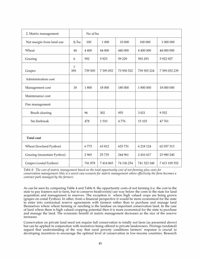
45

2. Matrix management No of ha

Net margin from land use $/ha 100 1 000 10 000 100 000 1 000 000

Wheat 44 4 400 44 000 440 000 4 400 000 44 000 000

Grazing 6 592 5 923 59 229 592 293 5 922 927

Grapes 7

395 739 505 7 395 052 73 950 522 739 505 224 7 395 052 239

Administration cost

Management cost 18 1 800 18 000 180 000 1 800 000 18 000 000

Maintenance cost

Fire management

Brush clearing 96 302 955 3 021 9 552

5m firebreak 478 1 510 4 776 15 103 47 761

Total cost

Wheat (lowland Fynbos) 6 773 63 812 625 731 6 218 124 62 057 313

Grazing (mountain Fynbos) 2 965 25 735 244 961 2 410 417 23 980 240

Grapes (costal Fynbos) 741 878 7 414 865 74 136 254 741 323 348 7 413 109 552

Table 8: The cost of matrix management based on the total opportunity cost of not farming plus costs for conservation management (this is a worst case scenario for matrix management where effectively the farm becomes a contract park managed by the farmer). As can be seen by comparing Table 4 and Table 8. the opportunity costs of not farming (i.e. the cost to the state to pay framers not to farm, but to conserve biodiversity) are way below the costs to the state for land acquisition and management in reserves. The exception is where high valued crops are being grown (grapes on costal Fynbos). In other, from a financial perspective it would be more economical for the state to enter into contractual reserve agreements with farmers rather than to purchase and manage land themselves where wheat farming or ranching is the landuse on important conservation land. In the case of land where there is high valued cropping potential then it is more economical for the state to purchase and manage the land. The economic benefit of matrix management decreases as the size of the reserve increases. Conservation on private land need not require full conservation to totally not farm (as presented above) but can be applied in conjunction with incentives being offered to private landowners. Perrings (undated) argued that understanding of the way that rural poverty conditions farmers’ response is crucial to developing incentives to encourage the optimal level of conservation in low-income countries. Research

46

conducted by Winter (2003) on landowner attitudes towards incentives for conservation, shows that an overwhelming majority of farmers were of the opinion that incentives were a good for promoting conservation on private land. Over 85% of the landowners questioned also regarded the protection of biodiversity outside of reserves as their responsibility, although, not as many respondents (over 35%) were prepared to bear the costs for that responsibility (Table 9) (Winter, 2003). More than 92 percent agreed that offering landowners incentives is a good idea for promoting conservation on private land.

Source: Winter (2003).

Note: N = 40 respondents.

Table 9: landowner attitudes towards incentives for conservation

Table 10 presents the attractiveness of incentives to landowners for promoting conservation on private land. Of the 14 incentive presented to private landowners, assistance with fencing and land management came first, followed by Assistance with alien vegetation clearing and third being rates relief for land conserved. Advice on legal compliance procedures and Public/community recognition came last. This response by private landowners shows that there is a high possibility of conservation on private land and private landowners will response positively to incentives. Therefore, incentives will foster conservation behaviour amongst private landowners.

∑

∑

Statement from questionnaire Agree (%)

Unsure (%)

Disagree (%)

Offering landowners incentives is a good idea for promoting conservation on private land

92.5 2.5 5

∑ Protection of plants and animals outside of reserves should be the responsibility of landowners

87.5 5 7.5

CNC or another government organization should bear the costs for the conservation of renosterveld property

57.5 7.5 35

47

Source: Winter (2003).

Note: N = 39 respondents.

Table 10: Attractiveness of incentives to landowners in the Overberg. Furthermore, when questioned about what prevents landowners from conserving more land on their property, 62% of the landowners sampled cited financial constraints as the reason, while only 5% of respondents considered the limitation to be management related. Matrix management would appear to be the most cost-effective mechanism for ensuring conservation in most circumstances. In essence the cost of managing the land for conservation will be the opportunity cost to the farmer of not using the land for the most profitable alternative land use activity minus the benefits that can be gained from the conservation based land use (e.g. tourism, cut flower sales). This cost will vary greatly, based on the most suitable land use options for the area. It will be very low for extensive rangelands, low for dryland grain production, but high for irrigated crops and speciality crops such as horticulture. In many instances, rangeland management is already biodiversity-friendly to many species, and to achieve the matrix management objective may require little or no intervention. Somewhat reduced stocking rates or minor changes in management practices (for instance, withholding grazing during a critical period) may be sufficient to achieve the desired results. Where dryland cropping is involved, a spatially-explicit strategic approach would be needed to ensure that viable biodiversity corridors are achieved. There are a multitude of mechanism through which matrix management could be supported including:

• Education of landowners. • Prestige-related incentives, including social recognition and peer-pressure.

• Financial incentives, such as rates reductions or direct payments. • Assistance with management costs associated with managing for biodiversity conservation (e.g

alien vegetation removal). Table 11 reports the results of a survey conducted among landowners in one of the affected areas, regarding the attractiveness of various incentives.

Incentive Percentage of

respondents (%)

Frequency

1. Assistance with fencing and land management 72.5 29

2. Assistance with alien vegetation clearing 67.5 27

3. Rates relief for land conserved 67.5 27

4. Grants or subsidies for conservation 65 26

5. Tax deductions 47.5 19

6. Access to scientific advice 45 18

7. Tourism incentives 40 16

8. Law enforcement 32.5 13

9. Access to farm planning and management support 32.5 13

10. Assistance with fire management 30 12

11. Free access to all WCNCB parks and reserves 27.5 11

12. Discounts for accommodation at WCNCB resorts 27.5 11

13. Advice on legal compliance procedures 17.5 7

14. Public/community recognition 15 6

48

Source: Winter (2003).

Table 11: Attractiveness of incentives to 39 landowners in the Overberg South Africa. Facilitated translocation

Costs for facilitated translocations cannot be compared directly with autonomous translocations, as the approach is only likely to be used where autonomous dispersal is not an option. The cost is very dependent on the type of organism, number of organisms translocated and the establishment costs involved. Simultaneous translocation of communities of mutually-interdependent organisms may have to be considered, including pollinators, and seed dispersers in the case of plants. Other than for large mammals, there is no current practice of translocation of biodiversity, and it is therefore difficult to estimate the costs that would be involved. Ex situ conservation

Gene-banking and other ex situ conservation are very unlikely to achieve the same level of biodiversity conservation as is achieved through in situ conservation, but remain a fall-back position when other opportunities are not available, and an insurance measure when they are. A common target for in situ is the conservation of at least 10% of the historical population. Ex situ conservation is likely to be able to conserve a small number of organisms for each species, therefore good representation of the genetic variation in the population is essential. Gene fingerprinting to ensure that the collection represents the broader population is therefore a significant cost consideration. Ex-situ conservation includes conservation in gene and/or seed banks, Zoo’s and botanical gardens. However, this paper only focuses on gene and seed banking. The data available for the costs of gene banking or seed banking is for research purpose only and should be applied as such. The costs of gene/seed banking are the costs incurred by the researcher during either DNA extraction or genetic fingerprinting, and collecting and recording seeds. Tables X7 shows in detail the costs of gene banking and seed banking.

Incentive Percentage of

respondents (%)

Frequency

1. Assistance with fencing and land management 72.5 29

2. Assistance with alien vegetation clearing 67.5 27

3. Rates relief for land conserved 67.5 27

4. Grants or subsidies for conservation 65 26

5. Tax deductions 47.5 19

6. Access to scientific advice 45 18

7. Tourism incentives 40 16

8. Law enforcement 32.5 13

9. Access to farm planning and management support 32.5 13

10. Assistance with fire management 30 12

11. Free access to all WCNCB parks and reserves 27.5 11

12. Discounts for accommodation at WCNCB resorts 27.5 11

13. Advice on legal compliance procedures 17.5 7

14. Public/community recognition 15 6

49

Costs per species (US$)

Number of samples

Gene banking 75 000 100 000 200 000 500 000 700 000

Start-up cost 26 620

Consumable cost per DNA extraction per species 22 1 679 104 2 238 806 4 477 612 11 194 030 15 671 642

Genetic fingerprinting for plants per fingerprint 30 2 238 806 2 985 075 5 970 149 14 925 373 20 895 522

Total cost 3 944 530 5 250 500 10 474 381 26 146 023 36 593 784

Seed banking Based on 7500 species

Average recording & collection costs Per species 184 1 376 865 1 376 865 1 376 865 1 376 865 1 376 865

Cost to re-establish plants in a plantation/ botanical garden per plant 1.49 111 940 149 253 298 507 746 268 1 044 776

Total cost 1 488 805 1 526 118 1 675 372 2 123 133 2 421 641

Table 12: The costs involved in ex-situ conservation. These costs are based on plants, but all biota need preservation. Large numbers of individual specimens over a range of locations would be needed for effective conservation.

Table 12 shows that the cost per DNA extraction per specimen is US$ 22 and for genetic fingerprinting is US$ 30. According to gene banking expert, it is anybody’s guess as to how many fingerprints need to be collected in order to sufficiently conserve/preserve a particular plant species. The operational and capital costs requirement for gene banking runs in excess of US$ 26 600. The average recording and collection costs per species are estimated at US$ 180 and the costs of re-establishing plants in plantation/ botanical garden costs per plant are estimated at US$ 1.49. This cost does not consider land acquisition for the botanical gardens, but assumes there is space. This may not be true if large numbers of species are involved.

50

5.4 Conclusions Adaptation options fall into two categories: adaptation option to conserve biodiversity in the natural habitat; and adaptation options to conserve biodiversity ex-situ in gene banks, zoos and botanical gardens. An economic comparison between these two options is not valid as it is a classic case of comparing apples and oranges. Conservation in natural habitats normally attempts to conserve 10% or more of the distribution of each species as well as the ecosystem processes. Ex-situ conservation only aims to conserve a minimum viable genetic sample of the population. Conserving biodiversity in the natural environments conserves not only the species, but the interaction between the species and the habitat, as well as ecosystem function. In addition thousands if not millions of individuals of a species may be conserves. Conserving species ex-situ is a last resource option when it is impossible to conserve the species in the natural habitat, and is also an insurance policy against unpredictable losses of species due to climate change or other impacts. Ex-situ conservation can only conserve a small number of individuals of any one species, and looses the conservation of symbiotic interactions between the conserves species and other species. Current models on both climatic and species responses to climatic change are still very crude and ignore many aspects. It is therefore impossible to predict with certainty which species will become extinct as a consequence of climate change and the safest option would be to try and set up a conserved genetic bank for all species. This cannot, however replace the need for conserving the species in its natural habitat wherever possible. From an economic perspective, the conservation of the matrix, i.e. those areas outside of the formal nature reserves is seen as the most cost effective mechanism to ensure protection of additional areas against consequences of climate change. The exception to this is when there is a high opportunity cost to conservation such as in areas with high valued agricultural crops such as grapes.

51

6 Capacity Building Outcomes and Remaining Needs A number of capacity building activities were conducted as a component of this research. The primary capacity building activity was the conducting of a four day course on tools and approaches to strategic conservation planning in a climatically changing environment. Details of this course are presented below. The course material has been prepared as a training file, and is also being set up as a self-training Web-based module hosted by the University of the Western Cape. This is available at the following web site http://planet.uwc.ac.za/nisl/AIACC. Aspects of this course have also been used in postgraduate training at the University of the Witwatersrand. Both the University of the Witwatersrand and the University of the Western Cape have expressed interest in using the course as a module in their postgraduate curricula next year. The following team members attended AIACC workshops and training sessions:

Workshop Participants Date

Nairobi. Global Kick-off Workshop

Bob Scholes 11-15 February 2002

Pretoria South Africa. Africa Regional Workshop

Bob Scholes Guy Midgely Barend Erasmus Jenny Cooper Graham von Maltitz Alet Visser Mike Rutherford

10 – 13 March 2003

Trieste Italy. Climate Change Vulnerability and Adaptation: AIACC Project Development Workshop

Jenny Cooper 3 – 14 June 2004

Dakar Senagal. Africa Regional Workshop

Graham von Maltitz Peter Novelli (stakeholder representative) Mark Botha (stakeholder representative)

Guy Midgely Alice Olwoch

24 – 27 March 2004

Belagio Italy. Vulnerability Workshop

Graham von Maltitz February 2005

Capacity building

The main capacity building component of this project was to run a training course on findings from our study, and to incorporate this into a web based training module. A report on the training course is given below.

52

Report on a short course on Tools and approaches to strategic conservation planning in a climatically changing environment: Ensuring sustainable protection of biodiversity in response to global climatic change using a strategic conservation planning approach.

University of the Western Cape, Cape Town, South Africa 22-25 February 2005

Assessments of Impacts and Adaptations to Climate Change (AIACC) is a global initiative developed in collaboration with the UNEP/WMO Intergovernmental Panel on Climate Change (IPCC) and funded by the Global Environment Facility (GEF) to advance scientific understanding of climate change vulnerabilities and adaptation options in developing countries. (http://www.start.org/project_pages/aiacc.html) AIACC project AF04 (Impacts and adoption to climatic change by the biodiversity sector in Southern Africa) presented a short course as a way of transferring the methods that had been developed during the project to the user community. The course was open to conservation planning professionals from South Africa, SADC countries, and a few participants from African and Indian Ocean countries. The course preparation was funded through the AIACC program. A supplementary grant from AIACC assisted with the costs of attendance by delegates from outside South Africa. In total 12 SADC delegates attended the course from the following 10 SADC countries. Botswana, Malawi, Namibia, Congo, Zimbabwe, Seychelles, Madagascar, Mozambique, Lesotho and Tanzania. In addition a further 17 participants and 7 presenters attended from South Africa, representing South African National Parks, South African National Biodiversity Institute, Council for Scientific and Industrial Research, Agricultural Research Council, Department of Water Affairs and Forestry, Gauteng Nature Conservation, Ezemvelo KZN Wildlife, the Maloti-Drakensberg Transfrontier Park, University of the Western Cape, University of the Witwatersrand and University of Stellenbosch. The objective of the course was to introduce participants to a number of tools that could be used to better understand impacts of climate change on biodiversity and how best to mitigate these impacts. Participants were introduced to datasets and methods in a hands-on approach using the computer facilities of the University of the Western Cape. Useful data and methods were presented to the participants on CD format to allow them to run their own assessments in their home institutions. A revised workshop manual, plus a multi-media pack including the lectures with voice-over from the presenters, is under preparation. Topics covered included:

• Introduction to workshop objectives (Dr Bob Scholes, CSIR Environmentek) • Climate change scenarios for Africa (Dr Bruce Hewitson, University of Cape Town) • Introduction to digital global change datasets (Mr Greg Hughes, South African National

Biodiversity Institute)

• Biodiversity responses to past changes in climate (Dr Guy Midgley, South African National Biodiversity Institute)

• Adaptation of biodiversity to climate change (Mr Graham von Maltitz, CSIR Environmentek) • Sources and limitations of African biodiversity data (Dr Belinda Reyers, CSIR Environmentek) • Review of datasets on computers (Dr Belinda Reyers, & Mr Greg Hughes) • Approaches to niche based modelling (theory and practical) (Dr Barend Erasmus, University of

the Witwatersrand, & Mr Greg Hughes)

• Putting dynamics into niche models. Demonstration (Dr Barend Erasmus, University of the Witwatersrand, & Mr Greg Hughes

• Field trip, where a climatic gradient experiment has been established on a mountain slope near Cape Town

• Ecosystem function under climate change (Dr Bob Scholes)

53

• Economic analysis of conservation response options to climate change (Mr Anthony Letswoalo, CSIR Environmentek)

• Implications for strategic conservation planning (Dr Belinda Reyers) • Closure (Dr Bob Scholes)

Overall a very positive response was received from all participants. The participants differed greatly in their need for training. To some the theory and background was most useful, whilst to others the actual hands on training was most useful. The participants from outside of South Africa, in particular, noted that they needed a longer exposure to the techniques in order to be able to apply them effectively, and that many of their colleagues would also benefit from the training. They urged a second round of training, preferably conducted in-country, so that a larger number of trainees could be reached. Remaining needs South Africa has extensive technical capacity to conduct further research into the impacts of climate change on biodiversity. Providing that funding is made available, it is likely that the South African Scientists will continue to develop world-class science that will expand our knowledge in this regard. Within South Africa the competence to interpret and implement these results at the National and Provincial level varies greatly between regions. The South African National Parks Board, as well as a few of the provincial parks boards have reasonable technical capabilities, but in the remaining parks boards there is limited capacity. Within SADC, with the possible exception of Namibia, the technical capacity to take this work forward is very limited. Out training was sufficient to introduce a number of individuals to the concepts and tools, but greater in country training was identified as a need by the workshop participants at our training course.

54

7 National Communications, Science-policy Linkages and Stakeholder Engagement

The following memorandum, based on AIACC activities in project AF04, was presented at a sitting of the National Cabinet of South Africa for consideration during 2004, and was revised in order to form the basis for a briefing paper for national team’s UNFCCC COP9 negotiations. This memo indirectly precipitated the increase in urgency in governmental concern in climate change threats to South Africa, and contributed to informing its negotiating position. Background

Acknowledging the uncertainty in the science of climate change prediction, but recognizing that uncertainty is reducing steadily as more evidence of unremitting climate change accumulates and as model projections increase in sophistication and credibility. Recognizing that IPCC Third Assessment Report findings increased the range of warming expected, and that very recent results raise these levels even more and suggest that future global warming of at least 2.4ºC is assured and up to as high as 11ºC could result from CO2 doubling from pre-industrial levels. Recognizing that these more extreme projections are likely to worsen the negative impacts projected by the SA Country Study on Climate Change, and therefore that this study requires urgent updating and broadening to a greater spread of potentially affected sectors. Implications for biodiversity Recent research carried out by the SA National Biodiversity Institute confirms SA Country Study results that climate change represents a real and significant threat to biodiversity in South Africa. South Africa’s biodiversity directly provides livelihoods for a significant portion of rural South Africans who are currently victims of poverty. Biodiversity also underpins a vibrant and growing source of revenue derived from the tourism and ecotourism industries. Maintenance of biodiversity is critical to the future economic well-being of these and many other stakeholders. New approaches to assessing climate change impacts (funded in significant part by Conservation International, Washington DC and the GEF-sponsored AIACC project) have allowed development of projections that address previously ignored complexity to derive credible future biodiversity scenarios, and to develop adaptation options. Potential impacts identified include the potential extinction of significant numbers of plant and animal species concentrated in the world-renowned winter rainfall biodiversity hotspots, especially those that are currently rare and those threatened by changes in land use. Other changes include shifts in the structure of vegetation, such as bush and tree encroachment into productive grasslands in summer rainfall regions, changes that threaten current use of ecosystem services and wildlife management strategies and that may cause erosion of biodiversity in the national protected areas estate which has been established and maintained at considerable cost. Adaptation options do exist, as long as the rate of climate change is not excessive, and range in their potential costs depending on the rate of climate change and ultimate point of stabilization. Natural adaptation by wild species and ecosystems is NOT sufficient to ensure the persistence of all biodiversity in the face of climate change in human-dominated landscapes – a hands-off approach will doom many species to extinction in the coming decades. Gene banking is a useful way of safely preserving some genetic variability of wild species, but in no way satisfies nature conservation requirements for functioning ecosystems. Active interventions to translocate species threatened by climate change to safer habitats in the wild are risky, costly and may be almost ineffective for plants, and appear viable only under exceptional circumstances (though more research is needed to assess this option more fully). Expansion of protected areas in targeted areas will be an important adaptation option, but a major viable alternative is to manage biodiversity with active collaboration between land-owners and conservationists to ensure as sympathetic a land use regime as possible to facilitate species persistence and natural migration. This strategy is an important outcome of new legislation contained in South Africa’s

55

Biodiversity Bill, which establishes bioregional planning as a legal requirement for regional development initiatives. The establishment of the SANBI to oversee bioregional planning activities is therefore a key contribution to climate change adaptation, in addition to its main aims and objectives. South Africa has thus established some of the most forward-looking strategies in this regard, which can contribute substantially to South-South initiatives to adapt to climate change in developing nations. This institutional capacity is supported by leading scenario development and modelling capability. Conservation International and AIACC funded activities have been central to the initial development of this world-leading capacity, and should be supported in further investments in capacity for adaptation to climate change in the developing world. Finally, with increasing climate change the range of adaptation options narrows, and costs increase until no strategy is economically or practically viable. It is therefore critical to support international efforts to limit greenhouse gas emissions as far as possible to ensure minimal further changes to climate and avoid increasingly dangerous levels of climate change. Two of the core research team Dr have been actively involved in representing South Africa on IPCC WG panels in the following capacities:

• Dr Bob Scholes: IPCC WG3 group on agriculture • Dr Guy Midgley IPCC WG2 on ecosystems. • In addition both Dr Scholes and Dr Midgley are part of the South African negotiating team

for UNFCCC meetings.

56

8 Outputs of the Project Peer reviewed journal publications Williams, P., Hannah, L., Andelman, S., Midgley, G.F., Araujo, M., Hughes, G., Manne, L., Martinez-Meyer, E. & Pearson, R. (in press) Planning for Climate Change: Identifying Minimum-Dispersal Corridors for the Cape Proteaceae. Conservation Biology Midgley, G.F., Hughes, G.O., Thuiller, W., Rebelo, A.G. (submitted) Migration rate limitations on climate change induced range shifts in Cape Proteaceae. Global Ecology and Biogeography Hughes, G.O., Thuiller, W., Midgley, G.F., Collins, K. (submitted) A fait accompli? Environmental change hastens the demise of the critically endangered riverine rabbit (Bunolagus monticularis). Biological Conservation Other outputs and papers in prep

van Jaarsveld, A.S., G.F. Midgley, R.J. Scholes, and B. Reyers. 2003. “Conservation management in a changing world.” In N. Allsopp, A.R. Palmer, S.J. Milton, K.P. Kirkman, G.I.H. Kerley, C.R. Hurt, and C.J. Brown, eds., Proceedings of the VIIth International Rangelands Congress, 26 July – 1 August 2003, Durban, South Africa. Hughes, G.O., Loehr, V.J.T., Thuiller, W., Midgley, G.F., Leuteritz, T.E.J. (in prep) Global change and an arid zone chelonian: The case of Homopus signatus: Environmental factors affecting modelled current and future distributions of Homopus signatus an arid zone chelonian endemic to South Africa. Letsoalo, A., Reyers, B., Hughes, G. Midgley, G. Maltitz, G.P. de Wit M (in Prep) Economic cost of alternative conservation response options to climate change: the case of Cape Floral Region (CFR) CSIR, Environmentek, Pretoria, South Africa. Midgley GF, B Erasmus, C Gelderblom, GO Hughes,, MJ Rutherford, RJ Scholes, A van Jaarsveld, GP von Maltitz, Authors (no order yet) (in Prep) Adapting biodiversity conservation strategy and practice for climate change. RJ Scholes1, G von Maltitz1, M de Wit1, GO Hughes2, G Midgley2 and B Erasmus3 (2004) Helping biodiversity adapt to climate change. SciDevNetwork Von Maltitz, G.P. Scholes, R.J., Erasmus, B. and Letsoalo, A. (in Prep) Adapting conservation strategies to accommodate impacts of climate change. Prepared for the AIACC Navasha, Kenya Adaptation workshop. Von Maltitz G. P. and Scholes, R. J. (in Prep) Vulnerability of Southern African Fauna and Flora to Climate Change. Paper prepared for the AIACC vulnerability workshop in Bellagion Italy.

57

9 Policy Implications and Future Directions

National issues

• Systematic biodiversity conservation needs to plan for changing climate and the impacts it will have on biodiversity. and not assume that the future will be like the past.

• Conservation biologists need to break from the old paradigm that species should only be located in areas where they historically occurred

• The protected area system can be configured to improve the protection it provides against climate change, including making provision for species movement.

• Off-reserve conservation needs to be increased, both as a cost effective way of increasing the impact of the reserve area, but also because climate change makes off reserve conservation more important.

• Policy makers need to consider the impacts of biodiversity loss on income and livelihood strategies to vulnarble groups.

• Given current economic and land use realities, it is unlikely that the protected area system can be sufficiently reconfigured to achive species conservation targets. Conservation authorities therefore need to maximize off reserve conservation, which is both cost effective and provides more spatial options.

Regional issues

• Tran-frontier movement of biodiverisity will be important given climate change. • As a result regional strategic conservation planning needs to consider park configuration to best

protect against the impacts of climate change. • Regional capacity building, especially in SADC countries other than South Africa is needed for

these countries to develop sufficient capacity to deal with adaptations to climate change. Global issues

• The cost to biodiversity, in both utilitarian and intrinsic terms, of anthropogenic climate change is high, and needs to be better understood and communicated.

Future directions and research needs

• Move from case studies to national strategic assessment. • Conduct sub-regional assessment of the level of threat. • Need to improve our scientific understanding on how individual species will responded to predicted climate changes.

• Need to scan for potentially threatened biota. • Undertake detailed studies on threatened genera. • Build capacity in SADC countries to conduct effective research and to undertake effective

adaptation relating to biodiversity and climate change.

58

10 References Allen, RG, LS periera, D Raes, and M Smith 1998 Crop evapotranspiration – Guidelines for computing

crop water requirements. FAO Irrigation and Drainage Paper 56, Food and Agriculture Organisation, Rome.

Austin, M.P., Nicholls, A.O., & Margules, C.R. (1990) Measurement of the Realized Qualitative Niche: Environmental Niches of Five Eucalyptus Species. Ecological Monographs, 60, 161-177.

Balmford, A. (2001) "Conservation Conflicts Across Africa." Science 291 (2001): 2616-19.

Balmford, A., Gaston, K.J., Blyth, S., James, A., and Kapos, V. 2003. Global variation in terrestrial conservation costs, conservation benefits, and unmet conservation needs. PNAS, VOL. 100, No 3.

Bowers, D.1997. Policy instruments for conservation of remnant vegetation: A British perspective. CSIRO Resource Futures Programme, Canberra.

Cain, M.L., Milligan, B.G., & Strand, A.E. (2000) Long-distance seed dispersal in plant populations. American Journal of Botany, 87, 1217-1227.

Calvete, C., Estrada, R., Angulo, E., & S., C.-R. (2004) Habitat factors related to wild rabbit conservation in an agricultural landscape. Landscape Ecology, 19, 531-542.

Cape Floristic Region. Biological Conservation, 112, 87-97. Cowling, R.M. & Pressey, R.L. (2003) Introduction to systematic conservation planning in the Cape

Floristic Region. Biological Conservation, 112, 1-13. Duthie, A.G. & Robinson, T.J. (1990). The African rabbits. In Rabbits, Hares and Pikas: Status Survey and

Conservation Action Plan (eds J.A. Chapman & J.E.C. Flux), pp. 121-127. IUCN/SSC Lagomorph Specialist Group.

Faith, D.P. & Walker, P.A. (1996) Integrating conservation and development: effective trade-offs between biodiversity and cost in the selection of protected areas. Biodiversity and Conservation, 5, 431-446.

Fielding, A.H. & Bell, J.F. (1997) A review of methods for the assessment of prediction errors in conservation presence/absence models. Environmental Conservation, 24, 38-49.

Frazee, S., Cowling, R.M., Pressey, R.L., Turpie, J.K., Lindenberg, N., 2003. Estimating the costs of conserving a biodiversity hotspot: a case study of the Cape Floristic Region, South Africa. Biological Conservation 112, 275–290.

Germishuizen, G. & Meyer, N.L. (2003) Plants of southern Africa: an annotated checklist National Botanical Institute, Cape Town, South Africa.

Glenz, C., Massolo, A., Kuonen, D., & Schlaepfer, R. (2001) A wolf habitat suitability prediction study in Valais (Switzerland). 55, 55.

Hewitson, B. (2003) Developing perturbations for climate change impact assessments. EOS, 84, 337-339.

Hoctor, T.S., Carr, M.H., Zwick, P.D., 2000. Identifying a linked reserve system using a regional landscape approach: the Florida Ecological Network. Conservation Biology 14, 984–1000.

Howard, B.M., Young, M.D., 1995. Selecting and Costing a Representative Expansion of the NSW Protected Area Network. CSIRO Resource Futures Programme, Canberra.

Hughes, L. (2000) "Biological Consequences of Global Warming: Is the Signal Already Apparent?” Trends in Ecology and Evolution 15, no.2.

James, A.N., Green, M.J., Paine, J.R., 1999. A Global Review of Protected Area Budgets and Staffing. World Conservation Monitoring Center, Cambridge.

Johnson, J.B. & Omland, K.S. (2004) Model selection in ecology and evolution. 19, 101.

Kerley, G.I.H., Pressey, R.L., Cowling, R.M., Bosho., A.F., Sims- Castley, R., 2003. Options for the conservation of large- and medium-sized mammals in the Cape Floristic Region. Biological Conservation 112, 169–190.

59

Lawler, J.J. & Edwards, T.C.J. (2002) Landscape patterns as predictors of nesting habitat: building and testing models for four species of cavity-nesting birds. Landscape Ecology, 17, 233-245.

Letsoalo, A., Reyers, B., Hughes, G. Midgley, G. Maltitz, G.P. de Wit M (in prep) Economic cost of alternative conservation response options to climate change: the case of Cape Floral Region (CFR) CSIR, Environmentek, Pretoria, South Africa.

Lewis-Winokur, V. & Winokur, R.M. (1995) Incubation temperature affects sexual differentiation, incubation time and posthatching survival in desert tortoises (Gopherus agassizi). Canadian Journal of Zoology, 73, 2091-2097.

Lineacre, ET (1977) A simple formula for estimating evaporation rates in various climates, using temperature data alone. Agricultural Meteorology 18, 409-429.

Loehr, V.J.T. (2002a) Diet of the Namaqualand speckled padloper, Homopus signatus signatus, in early spring. African Journal of Herpetology, 51, 47-55.

Loehr, V.J.T. (In Press) Diet of the Namaqualand Speckled Padloper (Homopus signatus signatus) revisited. Chelonian Conservation and Biology, Lunenberg.

Manel, S., Williams, H.C., & Ormerod, S.J. (2001) Evaluating presence-absence models in ecology: the need to account for prevalence. Journal of Applied Ecology, 38, 921-931.

Martin, R. 2003, Annual recurrent expenditure for conservation and management: A preliminary investigation of the use of a spreadsheet model to generate staff establishment and operating budget for individual parks. South African National Parks.

McCarty, J. P. "Ecological Consequences of Recent Climate Change." Conservation Biology 15, no. 2 (2001): 320-31.

McIntyre, S. and G.W. Barret. "Habitat Variegation, an Alternative to Fragmentation." Conservation Biology 6, no. 1 (1992): 146-47.

Midgley, G.F., Hannah, L., Millar, D., Thuiller, W., & Booth, A. (2003) Developing regional and species-level assessments of climate change impacts on biodiversity in theMurphy, H.T. and J. Lovett-Doust. "Context and Connectivity in Plant Metapopulations and Landscape Mosaics: Does the Matrix Matter?" OIKOS 105 (2004): 3-14.

Nakiccenovic, N et al (2000) Special Report on Emission Scenarios. Intergovernmental Panel on Climate Change, Geneva/ Cambridge University Press, Cambridge UK. 599pp.

Noss, R.F., Cooperrider, A., 1994. Saving Nature’s Legacy: Protecting and Restoring Biodiversity. Defenders of Wildlife and Island Press, Washington DC.

Palomares, F., Delibes, M., Revilla, E., Calzada, J., & Fedriani, J.M. (2001) Spatial ecology of the Iberian lynx and abundance of its primary prey, the European rabbit, in a heterogeneous environment. Wildlife Monographs, 148, 1-36.

Parmesan, C. and G. Yohe. "A Globally Coherent Fingerprint of Climate Change Impacts Across Natural Systems." Nature 421 (2003): 37-42.

Pearce, J. & Ferrier, S. (2000) Evaluating the predictive performance of habitat models developed using logistic regression. Ecological Modelling, 133, 225-245.

Pearce, J.L., Cherry, K., Drielsma, M., Ferrier, S., & Whish, G. (2001) Incorporating expert opinion and fine-scale vegetation mapping into statistical models of faunal distribution. Journal of Applied Ecology, 38, 412-424.

Pearson, R.G. & Dawson, T.P. (2003) Predicting the impacts of climate change on the distribution of species: Are bioclimate envelope models useful? Global Ecology and Biogeography, 12, 361-371.

Pence, G., Botha, M., Turpie, J.K., 2003. Evaluating combinations of on-and off-reserve conservation strategies for the Agulhas Plain, South Africa: financial perspective. Biological Conservation 112, 253–273.

Peters, R.L. & Darling, J.D. (1985) The green-house effect and nature reserves. BioScience, 35, 707.

60

Peters, R.L. (1991). Consequences of global warming for biological diversity. In Global climate change and life on Earth (eds R.L. Wyman), pp. 99-118. Chapman and Hall, New York.

Pickett, S.T.A., Thompson, J.N., 1978. Patch dynamics and the design of nature reserves. Biological Conservation 13, 27-37.

Press, D., Doak, D.F., Steinberg, P., 1996. The role of local government in the conservation of rare species. Conservation Biology 10, 1538–1548.

Pressey, R. L. and K.H. Taffs. "Scheduling Conservation Action in Production Landscapes: priority Areas in Western New South Wales Defined. Byirreplaceability and Vulnerability to Vegetation Loss." Biological Conservation 100 (2001): 355-76.

Pressey, R. L., R. M. Cowling and M. Rouget. "Formulating Conservation Targets for Biodiversity Pattern Andprocess in the Cape Floristic Region, South Africa." Biological Conservation 112 (2001): 99-127.

Pressey, R.L, Hager, T.C., Ryan, K.M., Scharz, J., Wall, S., Ferrier, S. & Creaser P.M. “Using abiotic data for conservation assessments over extended regions: quantitative methods applied across New South Wales, Australia.” Biological Conservation 96 (2000):55-82.

Programme. School of Bioresources Engineering and Environmental Hydrology, University of Natal, Pietermaritzburg, South Africa.

Rebelo, A.G. (2001) Sasol, Proteas, a field guide to the Proteas of Southern Africa, 2nd edn. Fernwood Press, Cape Town.

Reyers, B. "Incorporating Anthropogenic Threats Into Evaluations of Regional Biodiversity and Prioritisation of Conservation Areas in the Limpopo Province, South Africa." Biological Conservation 118 (2004): 521-31.

Root, T. L., J. T. Price, K. R. Hall, S. H. Schneider, C. Rosenzweig and A. J. Pounds. "Fingerprints of Global Warming on Wild Animals and Plants." Nature 421 (2003): 57-60.

Rouget, M., Richardson, D.M., & Cowling, R.M.C. (2003) The current configuration of protected areas in the Cape Floristic Region, South Africa - reservation bias and representation of biodiversity patterns and processes. Biological Conservation, 112, 129-145.

Rozemeijer and van der Jagt 2001. BOTSWANA CASE STUDY: Community-based natural resource management (CBNRM) in Botswana: How community-based is CBNRM in Botswana? In Schacklton and Campbell (eds) Empowering Communities To Manage Natural Resources: Case Studies From Southern Africa. USAID’s Regional Centre for Southern Africa’s “SADC NRM Project” The European Union’s “Action in Favour of Tropical Forests” and CSIR Pretoria.

Rushton, S.P., Ormerod, S.J., & Kerby, G. (2004) New paradigms for modelling species distributions? 41, 193.

Rutherford, M.C., Powrie, L.W., & Midgley, G.F. (2003) ACKDAT: a digital spatial database of distributions of South African plant species and species assemblages. South African Journal of Botany, 69, 99-104.

Rutherford. M.C. , Midgeley, G.F. Bond, W.J, Powrie, L.W., Roberts, R and L. Allsopp. 1999. Plant Biodiversity: vulnerability andadaptation assessment. South African Country Study on Climate Change. National Botanical Institute. Cape Town.

Sanderson, E.W., Jaiteh, M., Levy, M.A., Redford, K.H., Wannebo, A.V., & Woolmer, G. (2002) The human footprint and the last of the wild. BioScience, 52, 891-904.

Saunders, D.A., R. J. Hobbs and C. R. Margules. "Biological Consequences of Ecosystem Fragmentation: A Review." Conservation Biology 5, no. 1 (1991): 18-32.

Scholes, RJ (2003) Convex relationships in ecosystems containing mixtures of trees and grass. Environmental and Resource Economics 26, 559-574.

Scholes, RJ and Shackleton, CM (in prep) Controls on tree growth in South African savannas. J Applied Ecology.

61

Schulze, R.E. & Perks, L.A. (1999). Assessment of the impact of climate. School of Bioresources Engineering and Environmental Hydrology. University of Natal, Pietermaritzburg, South Africa.

Schulze, R.E. & Perks, L.A. (1999). Assessment of the impact of climate. Final report to the South African Country Studies Climate Change.

Schulze, R.E. (1997). South African atlas of agrohydrology and climatology. Water Research Commission Report TT82/96, Pretoria, South Africa.

Shafer, C.L., 1990. Nature Reserves: Island Theory and Practice. Smithsonian Institution Press, Washington, DC.

Swets, K.A. (1988) Measuring the accuracy of diagnostic systems. Science, 240, 1285-1293.

Terborgh, J., Estes, J.A., Paquet, P., Ralls, K., Boyd-Heger, D., Miller, B.J., Noss, R.F., 1999. The role of top carnivores in regulating terrestrial ecosystems. In: Soule´, M.E., Terborgh, J. (Eds.), Continental Conservation. Scientific Foundation of Regional Reserve Networks. Island Press, Washington DC, pp. 65–98.

Thuiller, W., Brotons, L., Araújo, M.B., & Lavorel, S. (2004) Effects of restricting environmental range of data to project current and future species distributions. Ecography, 27, 165-172.

Travis, J.M.J. (2003) Climate change and habitat destruction: A deadly anthropogenic cocktail. Proceedings of the Royal Society of London, series B, 270, 467-473.

Turpie, J., Winkler, H., Spalding-Fecher, R, Midgley, G. 2002. Economic impacts of climate change in South Africa: A preliminary analysis of unmitigated damage costs, Energy and Development Research Centre, University of Cape Town.

van Rensburg, B. J. and et al. "Conservation During Times of Change: Correlations Between Birds, Climate and People in South Africa." South African Journal of Scienc e 100 (2004): 266-72.

van Wilgen, BW (1986) A simple relationship for estimating the intensity of fire in natural vegetation SA J Botany 52, 384-385.

Walther, G. R., E. Post, P. Convey, A. Menzel, C. Parmesan, T. J. C. Beebee, J. M. Fromentin, O. Hoegh-Guldberg and F. Bairlein. "Ecological Responses to Recent Climate Change." Nature 416 (2002): 389-95.

Williams, p. Hannah, L., Andelman, S. Midgley, G., Araujo, M., Hughes, G., Manne, L, Marinez-Meyer, E. and R Pearson. Planning for climate change: identificying minimum-dispersal corridors from the Cape Proteaceae.

Williams, P.H., Moore, J.L., Kamden Toham, A., Brooks, T.M., Strand, H., D'Amico, J., Wisz, M., Burgess, N.D., Balmford, A., & Rahbek, C. (2003) Integrating biodiversity priorities with conflicting socio-economic values in the Guinean-Congolian forest region. Biodiversity and Conservation, 12, 1297-1320.

Winter, S. 2003. Attitudes and behaviour of landowners towards the conservation of renosterveld, a threatened vegetation types in the Cape Floral Kingdom, Unpublished Masters dissertation, University of Stellenbosch.

Young, M.D., Gunningham, N., 1997. Mixing instruments and institutional arrangements for optimal biodiversity conservation. In: Hale, P., Lamb, D. (Eds.), Conservation Outside Nature Reserves. Centre for Conservation Biology, University of Queensland, pp. 123–135.

Zimmerman, L.C. & Tracy, C.R. (1989) Interactions between the environment and ectothermy and herbivory in reptiles. Physiological Zoology, 62, 374-409.

(Page intentionally left blank)

For copies of final reports from the AIACC project and other information about the project, please contact:

AIACC Project Office

The International START Secretariat 2000 Florida Avenue, NW, Suite 200

Washington, DC 20009 USA Tel. +1 202 462 2213 Fax. +1 202 457 5859 Email: aiacc@agu.org

Or visit the AIACC website at:

www.aiaccproject.org