CBMS-FAO | 1

Impacts of Climate Change on Household Food Security in the Philippines

Celia Reyes, Joel Bancolita, Novee Lor Leyso and Steffie Joi Calubayan

December 2014

1. Introduction

The increasing complexity of shocks (global, economic and political crises, calamities and disasters, and

threats of climate change among others), and the limited, if not depleting capacities among poor and

vulnerable segments of the population to assessment that can be used as basis for better design and

implementation of policies and programs to mitigate and cushion the negative impacts of these shocks.

One of the emerging development concerns in recent years is that of the adverse implications of climate

change. In the Philippines, where extreme weather conditions during El Nino and La Nina is already

common, what makes climate change a threat in the country’s agriculture sector though is the undefined

shifting of climatic events such as rainfall, humidity and rising temperatures. This leads to the confusion of

farmers on when to plant especially without proper scientific guidance which in turn affects the food

security of the country.

Food security is defined as a state wherein all people have, at all times, physical, social and economic access

to sufficient, safe and nutritious food that meets their dietary energy requirements and food preferences for

an active and healthy lifestyle1. Being one of the goals of the agriculture sector under the Philippine

Development Plan (PDP) 2011-2016, the national government thru the Department of Agriculture launched

the Food Staples Sufficiency Program. Increasing productivity of the food staples such as rice corn, banana,

cassava and sweet potato, as well as rural income, is necessary in achieving food security and reduction of

poverty.

Appropriate policy measures need to be put in place to support the vulnerable population amidst problems

of growing poverty incidence aggravated further by the threats and impacts of climate change on food

security as well as on other human development outcomes. Consequently, it is important to examine

existing data that can facilitate the design of informed policy-decisions and well-targeted safety net

programs.

The community-based monitoring system (CBMS) is an important tool in monitoring the impacts of shocks

at the micro level. It can facilitate the conduct of vulnerability and risk assessment and mapping as it

generates the necessary disaggregated data (sub-national and household level data on socioeconomic

variables and poverty indicators) for identifying and profiling the vulnerable population. The system can

facilitate a better understanding of the nature and extent of exposure and vulnerability to shocks such as

that of climate-change and in examining their capacities to mitigate and cope with the adverse implications

of these shocks to their well-being and communities over time. Data from CBMS has been used in earlier

studies to examine the impacts on poverty of the increase in rice and fuel prices (Reyes, et al. 2009), of the

global financial crisis (Reyes, et al. 2010), and to monitor household coping responses during periods of

complex shocks.

This technical report aims to: (1) examine the nature and extent of vulnerability of households in the

Philippines to the impacts of climate change on food security; (2) profile vulnerable groups using available

data; (3) analyze available regional, provincial, municipal/city, and household level indicators of

1 FAO, Right to Food Glossary

CBMS-FAO | 2

vulnerability to food insecurity; (4) identify channels and indicators of the impacts of climate change on

food security; (5) and assess the relative efficiency of different policy tools or adaptation measures

simulating a range of policy options. To tackle these objectives, Section 2 elaborates on existing policies

and programs related to climate change’s impact on food security while Section 3 discusses related studies

on the topic. Section 4 tackles the methodology employed to generate the results presented in Section 5.

Finally, Section 6 discusses conclusion and recommendation.

2. Policies and Programs Addressing Climate Change’s Impacts on Food Security

2.1. National Climate Change Action Plan (NCCAP)

In 2009, Climate Change Act or Republic Act 9279 has been enacted to mainstream climate change into

government policy formulations and establish the framework strategy and program on climate change. This

act has also established an organizational structure called the Climate Change Commission. Its functions

include formulating a framework strategy and program which was translated into the National Climate

Change Action Plan in 2011 wherein one of the priorities is food security. Aside from that, the commission

is also involved in mainstreaming of climate risk reduction into national, sector and local development

plans and programs and recommending policies and key development investments in climate-sensitive

sectors.

The threat of climate change to food security in the Philippines has called the attention of the national

government to implement activities that will ensure availability, stability, accessibility and affordability of

safe and health food, which is the intermediate outcome of the plan. In order to achieve this, figure 1 shows

the immediate outcomes, as well as the outputs and the different activities that will be implemented until

2028:

CBMS-FAO | 3

Figure 1. Strategic Actions on Food Security for 2011-2028

Lifted from NCCAP Technical Document, 2011

The ability to provide adaptation measures that are well targeted and site-specific to the Philippine’s

food production sector is currently lacking which may be due to the lack of scientific information

on vulnerability and adaptation technologies. Given this, the NCCAP identified several activities

that will enhance the knowledge on the vulnerability of agriculture and fisheries.

First step in enhancing the knowledge on food production sector’s vulnerability is through the

“conduct of provincial-level vulnerability and risk assessments for agriculture and fisheries. In this

assessment, “site-specific adaptation and mitigation interventions including the research and

development agenda to test technologies and measures will be identified”. As of November 2011,

various studies have been conducted on vulnerability and risk assessments. According to the

Inventory of Methods for Climate Change Adaptation Project, a total of 40 studies have been

conducted so far which covered coastal and farming communities, crop specific studies on rice and

corn, and assessment of various watersheds found in the country.

The Philippines Research and Development Agenda in support of the NCCAP, did an initial

scoping of researches that might be classified under food security from the government agencies

and found out that food security, is ranked second with approximately 160 researches – with

Mindanao having the most number of researches. The following are some of the examples on

technical physical researches conducted:

CBMS-FAO | 4

Traditional rice landraces for wet and dry season cropping in Benguet (Benguet State

University)

Sweet potato cultivars for drought condition (Benguet State University)

Cruciferous vegetable production under water stress condition (Benguet State University)

Ecosystem based fisheries management to sustain fish catch (UP MSI

Installation of solar powered backyard aquaponics system for vegetable-tilapia-prawn-

catfish polyculture (CLSU-ICCEM)

On-farm plant genetic resources, conservation development and use for climate change

adaptation (Rice and Corn) (SeaRice)

Effect of CC on reproduction and early development of economically important

aquaculture species (SEAFDEC)

Hermetic Storage of rice seeds (PhilRice)

Rice Variety Development (drought tolerant, water submergence, salinity) (PhilRice)

However, gaps based from these researches were identified. Since rice and corn are the two most

important crops in the country, most VA studies focus on them only. Other gaps that were identified

are as follows: a.) lack of data on cost-effectiveness of mitigation and adaptation practices; b.) lack

of site-specific studies; c.) lack of harmonize VA tools with high precision; d.) lack of hatchery and

breeding techniques for marine species; e.) lack of interface with industry/community-based

enterprises to upscale research results; and f.) lack of enabling mechanisms to translate scientific

findings to policies. Furthermore, most of the studies on agriculture system and processes are land-

based which leaves the fishery sector less well understood.

After the researches are done, “studies and simulation models will be done based on the

vulnerability assessments and down-scaled climate scenarios, on the impacts of changing climates

on major crops, livestock and fisheries production. The research and development agenda sector

on climate change will be developed in order to conduct more specific short and long-term studies

on climate-resilient crop varieties, climate-smart crop, livestock management, and best practices.

These best practices will also be tested in fisheries and coastal management.”

The information that will be gathered from these studies will be developed and disseminated thru

the “climate information and database for agriculture and fisheries”. Lastly, “a resource network is

planned to be established wherein technical assistance on adaptation planning to local communities

and appropriate adaptation approaches to both men and women farmers and fishers can be

provided”.

A policy requiring the national and local governments to include climate change into their

respective plans and programs was passed in 2009. The NCCAP identified the formulation of

climate-sensitive agriculture and fisheries policies, plans and programs as one of its outputs in

ensuring food security. In order to achieve this, “the following activities are lined-up until 2028: a)

Integration of gender-responsive CC adaptation and mitigation in agriculture and fisheries plans,

programs, and budgets; and b) prioritization and enactment of a national land use law. The National

Land Use Bill will institutionalize land use and physical planning at the national and local levels,

and promote responsible and equitable allocation and administration of land and its corresponding

natural resources. Under the bill, critical areas (such as national parks, upland watershed areas, and

strategic agricultural and fisheries zones) will be identified and set aside.”

In order to enhance the social protection for farming and fishing communities the implementation

of risk transfer and social protection mechanisms for agriculture and fishery has been on-going via

the following programs:

CBMS-FAO | 5

Agrarian Reform Beneficiaries-Agriculture Insurance Program (ARB-AIP) A program being implemented by Department of Agriculture (DA) and Department of

Agrarian Reform (DAR) in partnership with the Philippine Crop Insurance Corporation

(PCIC) which aims to protect agrarian reform beneficiaries against losses due to pest and

disease infestations, natural calamities and extreme weather conditions brought about by

climate change. The national government allocated PhP 1 Billion for agricultural insurance

coverage of at least 224,036 agrarian reform beneficiaries nationwide.

Weather-index Based Insurance

It is an agriculture risk transfer mechanism for climate change adaptation and risk reduction

in the Philippines. Weather index insurance (WII) is a risk transfer instrument that pays

out compensation based not on actual losses experienced by an insured individual,

organization or institution, but once a weather index is triggered. After an extreme weather

event such as floods or drought, an insured person or organization is assured of immediate

compensation as long as a weather index is breached such as rainfall (if the amount of

rainfall exceeded the normal amount), wind speed (the velocity of the wind exceeded the

average wind speed passing through a particular locality) or dry days (number of days

without rain has exceeded the average within a municipality).

This program was just recently rolled-out in the Philippines by the Bankers Assurance

Corporation (BAC) under the name of Credit Asenso. It offers lending institutions security

for their operation or loan portfolio especially since the country is visited by typhoons at

least 20 times per year. Some of these fall within the trigger events defined by the product.

It uses a state-of-the-art satellite technology that determines event triggers for rainfall and

wind speed. This technology ensures that claims are determined on a real time basis or can

be viewed online thus there is no need for lengthy and time consuming claims

investigations and loss adjustments. Based on their location in the Philippines, trigger

indices for wind speed and rainfall have been developed for each municipality, which

makes it an innovative product in the Philippine’s micro-financing sector.

2.2. The Department of Agriculture Climate Change Program

Being the lead government agency in ensuring that the NCCAP’s listed outcomes on food security can be

achieved by 2028, the Department of Agriculture (DA) formulated specific programs and plans such as the

following:

“2.2.1. Climate Information System for Agriculture and Fisheries

It shall be established in different attached agencies to generate timely and reliable information to aid

in disaster risk reduction and management. Vulnerability and risk assessment mapping of productive

areas will be done wherein the map-based ex-ante analysis could be done before the onset of cropping

season. Aside from this, early warning systems will be established by improving meteorological

predictions in partnership with PAGASA. Improvement of agromet stations will be spread out not just

in regional/provincial level but also in major watershed, research centers, State Universities and

Colleges and other stations. Lastly, pest population surveys of the Bureau of Plant Industry will be

continued and a unit shall be established to develop predictive models to anticipate the resurgence of

pests.

This program has just finished its Climate Change Vulnerability Mapping under the National Irrigation

Authority (NIA) project and is currently undergoing project documentation for the release of funds.

2.2.2. Research and development for adaptive tools, technologies and practices

CBMS-FAO | 6

This is in line with the first expected output of the NCCAP which is to ensure site-specific knowledge

on the vulnerability of agriculture and fisheries. DA has outlined specific plans and programs such as

the following:

New designs and construction protocols for agri-fishery infrastructure that can withstand strong

winds, water intrusion and erosion, and other adverse impacts of the weather shall be developed.

Breeding and screening for climate resilient crops: crops suited to changing weather patterns

shall be developed such as early maturing crops, drought tolerant crops, crops that can

withstand limited as well as excessive moisture, etc.

Breeding and screening for heat tolerant livestock and poultry

Agro-reforestation: Species trials involving fruit and multipurpose trees shall be conducted on

representative upland watershed areas classified in accordance with the vulnerability and risk

assessment maps

Precision agriculture: Precision agriculture refers to a fine-tuned agricultural production that

takes into consideration planting dates based on weather predictions, planting design that

considers sun and wind exposures, varieties highly suited to the soil and weather patterns, and

the delivery of water and other inputs at the right time and at the right amounts. Research on

this area shall be done on a crop by crop or for livestock production and aquaculture

species/breed by species/breed basis as well as by location including urban areas

Urban agriculture: Vegetable farming especially during the rainy season in urban areas will

ensure reliable supply. There is a need to develop manageable vegetable farming systems on

urban structures as well as on limited urban spaces

Organic farming practices: There is need to develop crop varieties, livestock breeds and fish

strains suitable for organic production as well as effective organic inputs that will improve

productivity and make organic produce less expensive.

2.2.3. Fully engaged Extension System

This includes the following:

Early warning systems (EWS) for weather changesImprovedagri-fishery infrastructure

design standards and construction protocols

Soil moisture retention practices such as mulching, use of cover crops

Balanced fertilization

Organic farming tools and practices

Highly efficient farm irrigation methods such as drip irrigation for fruit trees, intermittent

irrigation for paddy rice, etc.

Credit and grants programs for climate change

Insurance programs for climate change

2.2.4.Repair and improvement of irrigation systems and establishment of SWIPS and SFRs

The National Irrigation Administration (NIA) with partner LGUs and irrigators associations shall see

that national and communal irrigation systems are repaired and improved upon to reduce leakage and

ensure efficient delivery of irrigation water at the right time and in the required amounts. SWIPS and

SFRs shall be established to maximize water harvesting and minimize losses.

As of 2012, the Corn Program of DA has already installed shallow-tube wells in areas with pronounced

dry season (Regions CAR, I, II and III). Aside from that, they have already facilitated supply of

alternative irrigation water especially during the El Niño phenomenon.”

2.3. Philippine Development Plan

CBMS-FAO | 7

Agriculture and Fisheries is one of the sectors included in the Philippine Development Plan for 2011-2016.

This sector being the provider of food and vital raw materials for the rest of the economy should be

competitive and sustainable. Two out of the three goals in order to achieve a competitive, sustainable and

technology-based agriculture and fisheries sector are the following:

“2.3.1. Improved security and increased rural incomes

One of the programs under this goal that is related to climate change is the establishment of climate resilient

agriculture infrastructure through enhanced technical design of irrigation and drainage systems and

facilities, farm-to-market roads (FMRs), postharvest facilities (PHF), trading posts, among others

2.3.2.. Increased sector resilience to climate change risks

In order to adapt to the threats of climate change and extreme weather events in the agriculture and fisheries

sector, sound scientific advice is needed regarding appropriate crop varieties, cropping patterns, and

climate-vulnerable structures, including irrigation systems. The following are the strategies in order to

achieve the goal in increasing resilience to climate change risks:

2.3.2.1. Reduce climate change-related risks and the vulnerability of natural ecosystems and

biodiversity through ecosystem-based management approaches, conservation efforts, and sustainable

environment and natural resources-based economic endeavors such as agri-ecotourism

2.3.2.2. Increase the resilience of agriculture communities through the development of climate change-

sensitive technologies, establishment of climate-resilient agricultural infrastructure and climate-

responsive food production systems and provision of support services to the most vulnerable

communities

2.3.2.3. Incorporate natural hazards and climate risk in the agricultural land use plan or the

Comprehensive Land Use Plan (CLUP)

2.3.2.4.Strengthen the capacity of communities to respond effectively to climate risks and natural

hazards

2.3.2.5. Continue vulnerability and adaptation assessments especially in food production areas”

2.4. Department of Agrarian Reform (DAR) Interventions on Climate Change Adaptation and

Mitigation

The Agrarian Reform Beneficiaries (ARBs) are not spared from the effect of the climate change. “It was

estimated that more or less 1M ARBs will be hit by climate change. The department have predicted the

following provinces, where most of their beneficiaries reside, to be flood-prone: Pangasinan, Pampanga,

Masbate and Leyte. On the other hand, the following provinces are predicted to be landslide-prone: Benguet,

Zambales, Nueva Vizcaya, Samar and Pangasinan. To minimize or completely eliminate the impacts of

climate change, DAR formulated mitigation and adaptation interventions”.

For their climate change adaptation, DAR will partner with various climate change implementing agencies

and institutions for training in climate change concepts and adaptation measures. There is also an “on-going

review and revision of Agrarian Reform Communities (ARC) Development Plans incorporating climate

change adaptation and mitigation. Under this, the following will be conducted: a.) development of tools for

assessment and planning; b.) conduct of consultation workshops. Another intervention is development of

the Crop-based Farmer Field School Curriculum and extension in coordination with farmer groups. Soil

and Water Conservation Technologies will also be introduced. One of the technologies to be introduced is

the Sloping Agricultural Land Technology (SALT). Organic Vegetable Growing is under this and as of

CBMS-FAO | 8

date, around 13, 622 ARBs in 259 ARCs are already adopting this practice. Lastly, susceptibility maps and

disaster preparedness materials based from the Mines and Geosciences Bureau and PAG-ASA.”

For the mitigation interventions, the following are the plans and programs that are currently being

conducted by the department or will be conducted in the coming years: “a.) National Greening Program ;

b.) Reduced Tillage Technology; c.) Integrated Farming Bio-System (IFBS) – it is the use of appropriate

environment-friendly and sustainable farming technologies and the provision of adequate extension and

support services. Around 16,161 are already adopters in 11 ARCs as of September 2011”.

3. Review of Related Literature

Food security

The UN’s Food and Agriculture Organization (FAO 2008), defines food security as a situation “when most

people are able, by themselves, to obtain the food they need for an active and healthy life, and where social

safety nets ensure that those who lack resources still get enough to eat” (Anbumozhi and Portugal, 2011,

p.5). The FAO identifies four main dimensions of food security: physical availability of food, economic

and physical access to food, food utilization and stability of the other three dimensions over time. According

to the FAO, “for food security objectives to be realized, all four dimensions must be fulfilled simultaneously”

(FAO, 2008).

Echoed by Anbumozhi and Portugal (2011), they argue that in looking at food systems these four

dimensions of food security identified by FAO should be taken into consideration. Food availability refers

to the global and regional food supply. Food accessibility on the other hand refers to the ability of

individuals to purchase food in sufficient quantities and quality. Food stability refers to the maintenance of

the continuity of food supply of seasonal production, while food utilization refers to the food consumption

patterns, malnutrition, pest contaminations, diseases and people’s capacity to obtain necessary nutrients

from the food they consume.

Building on the FAO definition of food security, Pinstrup-Andersen (2009) suggests that “a household is

considered food secure if it has the ability to acquire the food needed by its members to be food secure”.

He makes a distinction between transitory and permanent food insecurity, where the former describes

“periodic food insecurity as for example seasonal food insecurity, while the latter describes a long-term

lack of access to sufficient food”. He adopts the USDA measure of household food security which “is based

on household self-declarations, differentiates between low and very low food security…on the household-

level resource constraints” (i.e. does the household have the resources to acquire the food needed?).

Ziervogel, et al. (2006) looked at food security in terms of availability, access, utilization, and livelihoods.

They argue that a livelihoods understanding in defining food security is useful because “it emphasizes the

importance of looking at an individual’s capacity for managing risks, as well as the external threats to

livelihood security, such as drought” (p.8).

According to Anbumozhi and Portugal, “Food security can be evaluated under two different perspectives:

from a micro and a macro level. The micro-level food security refers to household and individual levels

and evaluates the nutritional well-being of individuals, whereas the macro-level food security focus at a

national policy level and assesses regular supplies of food in national, regional, and local markets.” (p.5).

FAO refers to vulnerability in terms of food security as the “group of factors that places people in a situation

where they are at risk of food insecurity, including factors that undermine people's capacity to deal with the

situation” (FAO, 2000).

CBMS-FAO | 9

Lovendal and Knowles (2006) linked food security and vulnerability in their research. They provide a

definition of vulnerability in terms of food security. They define vulnerability “relative to the negative

outcome of food security and define as vulnerability people’s propensity to fall, or stay, below the food

security threshold within a certain time frame”. They offered a framework for understanding food security

by including risks and the ability at different levels to manage these to reduce the probability of people

being food insecure in the future. The suggested framework looks at present characteristics of food security

status, risks such as shocks, trends and seasonality, and risk management to predict future food security

status which is measured by food availability, access to food, food consumption, food utilization and

nutritional status.

Figure 2. Framework for vulnerability to food security

Source: Lovendal and Knowles, 2006

At the macro-level, according to the ADB report on Food Security and Climate Change in the Pacific (2008),

the factor influencing food security include food importation, global food and fuel prices, disasters and

Pre

sen

t ch

arac

teri

stic

s

Risks

(Shocks, trends,

seasonality)

Type

Level

Frequency

Timing

Severity

Risk

management

Actors

Level

Market/non-

market

Ex ante/ex post

Food

availability

Access to

food

Food

consumption

Food

utilization

Nu

trit

ion

al s

tatu

s

Present food

security status to

Events to-t1 Expected future food

security status

t1

Food consumption ( FIES)

Malnutrition prevalence (CBMS)

CBMS-FAO | 10

emergencies, and factors such as traditional and subsistence agriculture, land and water resources, increased

urbanization and globalization, technological constraints to agricultural production and private investment

on agricultural production.

Echoing the importance of looking at food importation, Gingrich, et al. (2001) showed in their study that

foreign exchange availability greatly affects food security in food-importing countries such as Indonesia

and the Philippines. They argue that a combination of foreign exchange supplies, cereal prices and domestic

cereal production determine the relative cost of food security imports. One implication, according to them,

is that both countries should further diversify their export sectors to help stabilize export revenues.

On the other hand, Hoddinott and Yohannes (2002) suggest an alternative measure of food security. Using

data from India, the Philippines, Mozambique, Mexico, Bangladesh, Egypt, Mali, Malawi, Ghana, and

Kenya, they suggested using dietary diversity as an alternative measure because of four reasons, “1) a more

varied diet is a valid outcome in its own right; 2) a more varied diet, either directly or indirectly through

improved acquisition of micronutrients, is associated with a number of improved outcomes in areas such

as birth weight, child anthropometric status, improved hemoglobin concentrations, reduced incidence of

hypertension, reduced risk of mortality from cardiovascular disease and cancer; 3) such questions can be

asked at the household or individual level, making it possible to examine food security and the household

and intra household levels and 4) obtaining these data is relatively straightforward”.

They define dietary diversity as the number of unique foods – foods were divided into categories: basic

staples, luxury staples, vitamin-A rich, other roots and tubers, other fruits, other vegetables, beverages,

spices and others. This was included with four other indicators of food security (per capita expenditures,

caloric availability, caloric availability from staples, and caloric availability from non-staples). They

concluded that the use of dietary diversity as an alternative measure is feasible and has uses.

Gittelson, et al. (1998) note that while “food security has long been used as an important macro-level

indicator of agricultural stability and progress for both agricultural and economic researchers, little work

has been done to operationalize the concept at the household level” (p.210). They argue that household food

security as a concept should integrate “environmental, economic, and cultural factors” (p.210).

Sanchez (2000) suggests an integrated natural resource management approach that aims to address issues

of food security while addressing poverty reduction while satisfying societal objectives for environment

protection. The approach includes “identifying and quantifying the extent of food insecurity, rural poverty

and resource degradation problems to be addressed in a given region, enhancing the direct utilitarian

functions of natural resources, which consist of food, raw materials and income in the case of agriculture,

enhancing the ecosystem functions of natural resources, such as carbon, nutrient and water cycling, erosion

control and biodiversity, assessment of trade-offs between the options that enhance the food and income

functions of systems and those options that enhance the ecosystem functions” and dissemination.

Webb, et al. (2006) expands the discussion on how to measure food security by suggesting a more

qualitative approach. They suggest that measures for food insecurity should “1.) shift from using measures

of food availability and utilization to measuring “inadequate access” (key to access is purchasing power

and varies in relation to market integration, price policies and temporal market conditions) ; 2.) shift from

a focus on objective to subjective measures; and 3.) emphasize fundamental measurement as opposed to

reliance on distal, proxy measures”.

Building on the FAO definition of food security Napoli (2010) notes that “an integral part of the multi-

dimensional nature of food security is the nutritional dimension” (p.19) and that as mentioned earlier food

security consists of four essential parts: food availability, food access, food utilization and stability.

CBMS-FAO | 11

On the other hand, the United States National Food Security Measure employs a more micro-level approach

by looking at the dietary intake, nutritional status and physical well-being of individuals. The measure also

assesses the “cognitive and affective components of uncertainty, unacceptability or unsustainability”

(Wolfe and Frongillo, 2001, p.6) such as insecurity over future intake. Growth status is also used as an

indicator, as well as precursors to food security such as income, total expenditure, and coping strategies.

Wolfe and Frongillo (2001), in this regard, suggest that the experience of food insecurity itself is an

important measure.

Anriquez, et al. (2012) offers a “guideline to construct household specific dietary energy requirements, in

a way which is consistent both with the different needs of populations according to their physical

constitution, age and gender; and consistent with the way FAO calculates energy requirements”. They

suggest that to be able to determine which household or individual is food insecure and to be able to quantify

food energy gap, “actual household (individual) calorie intake should be compared with a relevant energy

requirement threshold” which quantifies the necessary (minimum) or the recommended (average) energy

requirement, to balance the energy expenditures needed to maintain body size and composition, and a level

of necessary (minimum) or desirable (average) physical activity that is consistent with good health in the

long run (Anriquez, et al., 2012).

Sarris and Karfakis (2010) developed a measure of rural household vulnerability which estimates

idiosyncratic shocks. The methodology “integrates a major source of covariate shocks, with established

techniques for estimating idiosyncratic shocks to estimate vulnerability of rural households in two regions

of Tanzania”. The findings suggest that the “major covariate risk relates to weather induced production

variations as well as price variations that give rise to agricultural income variations” which make

households vulnerable and forces them to adopt strategies such as “income and crop diversification” and

“consumption smoothing strategies”.

Capaldo, et al. (2010) proposed a vulnerability model to food security that sees vulnerability “result of a

recursive process: current socio‐economic characteristics and exposure to risks determine households’

future characteristics and their risk‐management capacity. This framework builds on the framework put

forward by Lovendal and Knowles (2006) (see Figure 2).

The Food Insecurity and Vulnerability Information and Mapping System (FIVIMS) is broadly defined to

“include any information system – or network of systems – that monitors the situation of people who are

poor or vulnerable to transitory and/or chronic food insecurity”. According to Weissman, et al., (2002), the

FIVIMS “are networks of systems that assemble, analyse and disseminate information about the problem

of food insecurity and vulnerability” which aims to raise awareness about food security issues, improve the

quality of food security-related data and analysis, promote donor collaboration on food security information

systems at country level, encourage better action programmes on poverty and hunger, and to improve access

to information through networking and sharing” (p.278). According to Fresco and Baudoin (2002), “at the

international level, FIVIMS implements diverse activities in support of national information systems, to

enable them to become part of an international information exchange network” and “at the country level,

FIVIMS works with a network of information systems that gather and analyse relevant national and sub-

national data that measure food insecurity and vulnerability.

Building on the FIVIMS, Devereux, et al. (2004) proposes a FIVIMS Integrated Livelihoods Security

Information System’ (FILSIS) which supports a “two-track approach to fighting both food insecurity (i.e.

dealing with shocks) and underlying household income poverty (i.e. strengthening livelihoods)” and

focuses on livelihoods rather than poverty. Devereux, et al. (2004) suggests that a livelihood approach to

food security “might provide a practical toolkit for linking the analysis of food insecurity with a multi-

dimensional and people-centred analysis of poverty – looking beyond income and consumption levels to

include an assessment of people’s strategies, assets and capabilities”.

CBMS-FAO | 12

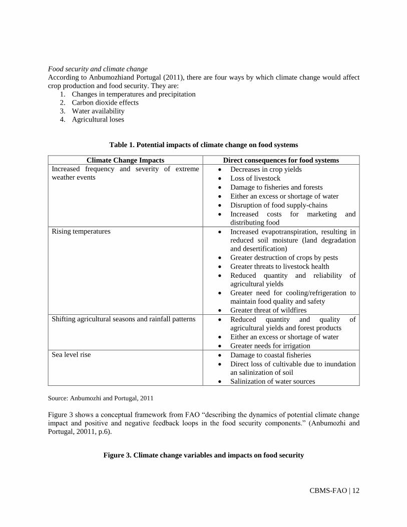
Food security and climate change

According to Anbumozhiand Portugal (2011), there are four ways by which climate change would affect

crop production and food security. They are:

1. Changes in temperatures and precipitation

2. Carbon dioxide effects

3. Water availability

4. Agricultural loses

Table 1. Potential impacts of climate change on food systems

Climate Change Impacts Direct consequences for food systems

Increased frequency and severity of extreme

weather events Decreases in crop yields

Loss of livestock

Damage to fisheries and forests

Either an excess or shortage of water

Disruption of food supply-chains

Increased costs for marketing and

distributing food

Rising temperatures Increased evapotranspiration, resulting in

reduced soil moisture (land degradation

and desertification)

Greater destruction of crops by pests

Greater threats to livestock health

Reduced quantity and reliability of

agricultural yields

Greater need for cooling/refrigeration to

maintain food quality and safety

Greater threat of wildfires

Shifting agricultural seasons and rainfall patterns Reduced quantity and quality of

agricultural yields and forest products

Either an excess or shortage of water

Greater needs for irrigation

Sea level rise Damage to coastal fisheries

Direct loss of cultivable due to inundation

an salinization of soil

Salinization of water sources

Source: Anbumozhi and Portugal, 2011

Figure 3 shows a conceptual framework from FAO “describing the dynamics of potential climate change

impact and positive and negative feedback loops in the food security components.” (Anbumozhi and

Portugal, 20011, p.6).

Figure 3. Climate change variables and impacts on food security

CBMS-FAO | 13

Source:Anbumozhi and Portugal, 2011

Lobell, et al., looked at crop specifically to assess the impacts of climate change on food security. According

to Lobell, et al. (2008), “crops which have relative strong dependence of historical production on rainfall

were considered cases with uncertainties” suggesting that it is not sure whether or not climate change would

have effect on these crops).”To ascertain which crops would most likely be affected by climate change,

they expressed the need for more precise projection of rainfall. Finally, they suggested putting investment

(prioritize) on crops that will be least affected by climate change, not a simple changing of planting dates

or shifting to other crops.

In an earlier work, Rosenzweig and Parry (1994) looked at the potential effects on agricultural production

(and hence food security) of climate change. They used a world food trade model to simulate the economic

consequences of potential changes in crop yields to estimate changes in world food prices and in the number

of people at risk of hunger. One finding is that there seems to be a big disparity between developed and

developing countries in terms of agricultural vulnerability. General Circulation Models (GCMs) were tested

in terms of CO2 levels, yield changes estimates, and farm-level adaptations. Adaptation included were

changes in planting date, variety, crops, and applications of irrigation and fertilizer. In the world food trade

model, it is predicted that in the climate change scenario, without direct CO2 effects, world cereal

production would be reduced by 11 to 20 percent. Upon inclusion of CO2 effects, yield decreases between

1 to 8 percent. Price increases are estimated to be between ~24-145 percent and the number of hungry

people would increase by ~1 percent for every 2-2.5 percent increase in prices. People at risk of hunger

increase by 10 percent to almost 60 percent. Upon inclusion of farm adaptation in the world food trade

model, world production levels are restored.

Scenarios near the high end of the IPCC range of doubled CO2 warming exerted slight to moderate negative

on cereal production. The only scenario that yielded positive cereal production was one involving major

and costly changes in agricultural systems (i.e., installation of irrigation). In sum, climate change is found

to increase disparities in cereal production between developed and developing countries.

Building on Rosenzweig and Parry (1994), Parry, et.al (2004) suggests that changes in regional crop yields

under each scenario are the result of the interactions among temperature and precipitation effects, direct

physiological effects of CO2, and effectiveness and availability of adaptations.

Arnell, et al. (2004) on the other hand suggests that “the future impacts of climate change will depend to a

large extent on the future economic, demographic, social and political characteristics of the world”. The

paper downscaled the IPCC’s Special Report on Emissions Scenarios (SRES) world-region population and

Drivers of

Global

Warming

Climate change variables:

-CO2 fertilization effects

-Increase in global mean

temperature

-Gradual changes in

precipitation

-Increase in frequency of

extreme weather events

-Greater weather variability

Adaptive response

of food systems

Changes in

food system

assets

Changes in

food system

activities

Changes in

components of

food security

Possible changes in

food consumption

patterns

Possible

changes in

human health

Possible changes

in nutrition status

CBMS-FAO | 14

economic data scenarios to the national and sub-national scales for a global climate impact assessment of

future food scarcity, water stress, exposure to malaria, coastal flood risk and wetland loss and terrestrial

ecosystems. They suggested that urban and rural growth rates be considered. Two limitations of the SRES

scenarios were identified: first, “there are considerable difficulties involved in moving from the scale at

which the SRES scenarios were produced (11–13 world regions) to the much finer spatial resolution

required by impacts models. A number of rather major assumptions had to be made, most specifically that

all parts of a region would change at the same rate: this was applied to population, GDP and land cover”

and; second, “whilst the SRES land cover trends are consistent with the narrative storylines, they are

inconsistent with recent trends. Under none of the storylines is there a sustained continued deforestation,

for example, and crop areas decrease under all of them”.

Ziervogel and Eriksen (2010) offer a framework for assessing the impacts of climate change on food

security. They discussed linkages between climate change (temperature, precipitation, and extreme

weather events), food security (availability, accessibility, stability and utilization) and its drivers (cycles

for consistency, agricultural management, socio-economic variables, demographic change, cultural and

political variables and science and technology).

Figure 4. Linkages between climate change and food security

Source: Chart taken from Ziervogel and Eriksen, 2010

According to them, the key issues that should be addressed to respond to food insecurity and managing

transitions or innovation in cropping system include: chronic poverty, functioning markets, farmer attitudes

toward managing risks, and reforming or improving the institutions responsible for managing food and

agricultural systems.

In the Philippines, the Department of Agriculture expects the following impacts of different climatic events

as shown in the table 2:

Table 2. Expected impacts of global climate change in the Philippine agricultural sector

No Climatic Events Impact Source/Assumptions

1 Rainfall Decrease by 20 percent, but

increase in intensity. Increase

IPCC 2007

Godilano, E.C. 2005

FAO (2006)

Climate change

Temperature

Precipitation

Extreme weather

events

Food security drivers

Cycles for consistency

Agricultural management

Socio-economic variables

Demographic change

Cultural and political variables

Science and technology

Food security

Availability

Accessibility

Stability

Utilization

CBMS-FAO | 15

risk of soil erosion and

occurrence of landslides.

2 Rainy Days Decrease rainy days but intensity

will be higher than normal,

growing periods may shorten by

approximately 30 days

Rosenzweig and Parry,

1994

IPCC 2007

3 Cyclone Increase intensity and occurrence

and may trigger landslides and

flooding of coastal areas.

IPCC 2007

4 Maximum temperature Increase by three percent, more

frequent and persistent El Niño

episodes, and increased

evaporation. Crop duration

shortened between one and four

weeks. Drought will be longer

and more intense, heat waves

occurrence.

IPCC 2007

NOAA, 2007

5 Flooding Increase flooding depth,

frequency, intensity, and severe

landslides. Submergence of

coastal communities and coastal

erosion

IPCC 2007,

Brackenridge, G.R. and

Anderson, E. (2004)

Dartmouth Flood

Observatory USA (2009)

6 Ground Water Potential

(GWP)

Decrease water availability, poor

quality, and salt intrusion

IPCC 2007

Godilano, E.C. 2005

8 Cloudiness Increase in total cloud cover,

decrease photosynthesis. Clouds

regulate the amount of sunlight

received by the surface and so

influence evaporation from the

surface, which in turn influences

cloud formation

NOAA, 2007

NASA Water Vapor

Project (NVAP) 1992

Source: Department of Agriculture Policy and Implementation Program on Climate Change

Impacts on crops

As to how the production of crops would be affected most by climate change, results vary. Most argue,

however, that climate change would affect different crops differently. Lobell and Field (2007) note that for

crops that rely too much on water such as rice and soybean, precipitation would be key in explaining the

effect of climate change but for other crops, temperature should be considered.

In the Philippines, agricultural production, according to Buan, et al. (1996), is “traditionally concentrated

on a few main crops [with] rice and corn [as] the major food crops” (p.42) and corn acts as a major substitute

for rice especially for Central Luzon and “is the main ingredient for livestock feeds, food products, and is

important in industrial uses.” (p.42). On the other hand, “coconut and sugarcane are the major commercial

crops that constitute important export commodities” (p.42). Buan, et al. (1996) note that both rice and corn

CBMS-FAO | 16

crops are “highly vulnerable to climate variability”. Climate-related occurrences have historically affected

rice and corn production losses between 1968 and 1990 according to Buan, et al. (1996). The study showed

that for all scenarios there will be consistent decrease in corn yield, while for rice, results were rather more

varied.

In a study on the relationship between yields for soybean and corn and climate trends, Kucharik and Serbin

(2008) noted that temperature and precipitation both affected corn yields while for soybean yields,

precipitation “had a slightly larger impact on the overall multiple regression results” (p.7).

Alexandrov, et al. (2002) also note the varied impacts of climate change on different crops. They showed

that “the increase in simulated soybean seed yield for the next century was caused primarily by the positive

impact of warming and especially by the beneficial direct CO2 effect” (p.379). On the other hand, decrease

in the winter wheat yield “was caused primarily by a shortened growing season owing to projected warming

and some increases in precipitation during the crop-growing season” (p.379). However, increasing the level

of CO2 in the scenarios showed an increase in the yield of winter wheat. Comparing the two, if the CO2

levels increase, soybean yield will show a decline and winter wheat yield will increase.

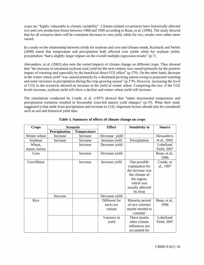
The simulations conducted by Conde, et al. (1997) showed that “under incremental temperature and

precipitation scenarios resulted in favourable (rain-fed maize) yield changes” (p.19). What their study

suggested is that aside from precipitation and increase in CO2, important factors should also be considered

such as soil and historical yield data.

Table 3. Summary of effects of climate change on crops

Crops Scenario Effect Sensitivity to Source

Precipitation Temperature

Winter wheat Increase Increase Decrease yield Alexandrov,

et al., 2002 Soybean Increase Increase Increase yield Precipitation

Wheat,

maize, barley

Increase Decrease yield Lobelland

Field, 2007

Corn Increase Decrease yield Buan, et al.,

1996

Corn/Maize Increase Increase yield One possible

explanation for

the increase was

the climate of

the region,

which was

usually affected

by frost

Conde, et

al., 1997

Increase Decrease yield

Rice Different for

each rice

variant

Maturity period

of rice varieties

maybe needed to

consider

Buan, et al.,

1996

Variance in

yield

There maybe

other climate

influences not

accounted for

Lobelland

Field, 2007

CBMS-FAO | 17

Increase

(minimum

temperature

in July-

August)

Increase/Decr

ease in July –

August

Increase yield But in general

an increase in

temperature by

as small as 0.3C

is associated

with a decline in

yield, though

there may be

increase in yield

if temperature

increase by 1.5C

and 3.0C,

demand for

irrigation water

would be

induced (evapo-

transpiration

Mahmood,

et al., 2012

Increase

(maximum

temperature

in July-

August)

Decrease yield

Decrease

(minimum

temperature

in September-

October)

Increase yield

Decrease

(maximum

temperature

in September-

October)

Decrease yield

Decrease

(min and max

temperatures

in September-

October)

Increase Decrease yield

Adaptation to climate change

A survey of the literature showed that oft-cited short-term adaptation strategies include “changes in planting

dates and cultivars; changes in external input such as irrigation; techniques in order to conserve soil water”

(Alexandrov, et al. (2002), p.383). For example, for Austria, Alexandrov, et al. (2002) suggested that spring

crops be sown earlier “in order to reduce yield loss or to further increase the projected gain resulting from

an increase in temperature” (p.384).

Conde, et.al (1997) assessed the potential increase in production costs as a result of the implementation of

adaptive measures to reduce climate change impacts. They suggested fertilization as a measure for adapting

to climate change in Mexico. However, they noted the importance of subsidies from governments to be able

to continue both maize production and fund the use of fertilizers. However they also noted that “under a

non-subsidy policy, the application of this adaptive measure would become unfeasible due to the high

production costs involved, since profits would be reduced and losses could even occur” (p.21).

Burke and Lobell (2010), on the other hand, differentiated between ex-ante and ex-post measure. While ex-

ante measures refers to the action taken in “anticipation of a given climate realization” which often center

around diversification of crops among others, ex-post measures are responses “undertaken after the event

is realized” which include “drawing down cash reserves or stores of grain, borrowing from formal or

informal credit markets or family, selling assets such as livestock, or migrating elsewhere in search for

work in non-affected regions” (p.135). However, Burke and Lobell (2010) argued that not all strategies for

adaptation are available to farmers. They noted that “existence of social safety nets and functioning financial

CBMS-FAO | 18

markets ensure that farmers are either insured against losses, can borrow around them, or can receive help

from the government to maintain livelihoods during bad times” (p.135).

4. Methodology

The methodology builds on the framework of Lovendal and Knowles (2006) and the study by Karfakis, et

al. (2010). Consistent with the literature, food insecurity will be measured in terms of (1) food expenditure

and (2) malnutrition. Correspondingly, two datasets are employed, namely: the 2009 Family Income and

Expenditure Survey (FIES) and the 2007-2010 pooled Community Based Monitoring System (CBMS) data

of 16 provinces. The model specification and estimation methodology will depend on the available

variables and measure of food security available from each of the datasets. The following subsection

presents the matching of variables across different surveys with the variables used by Karfakis, et al (2010)

in their study.

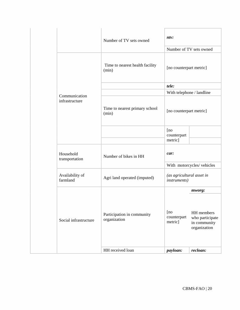
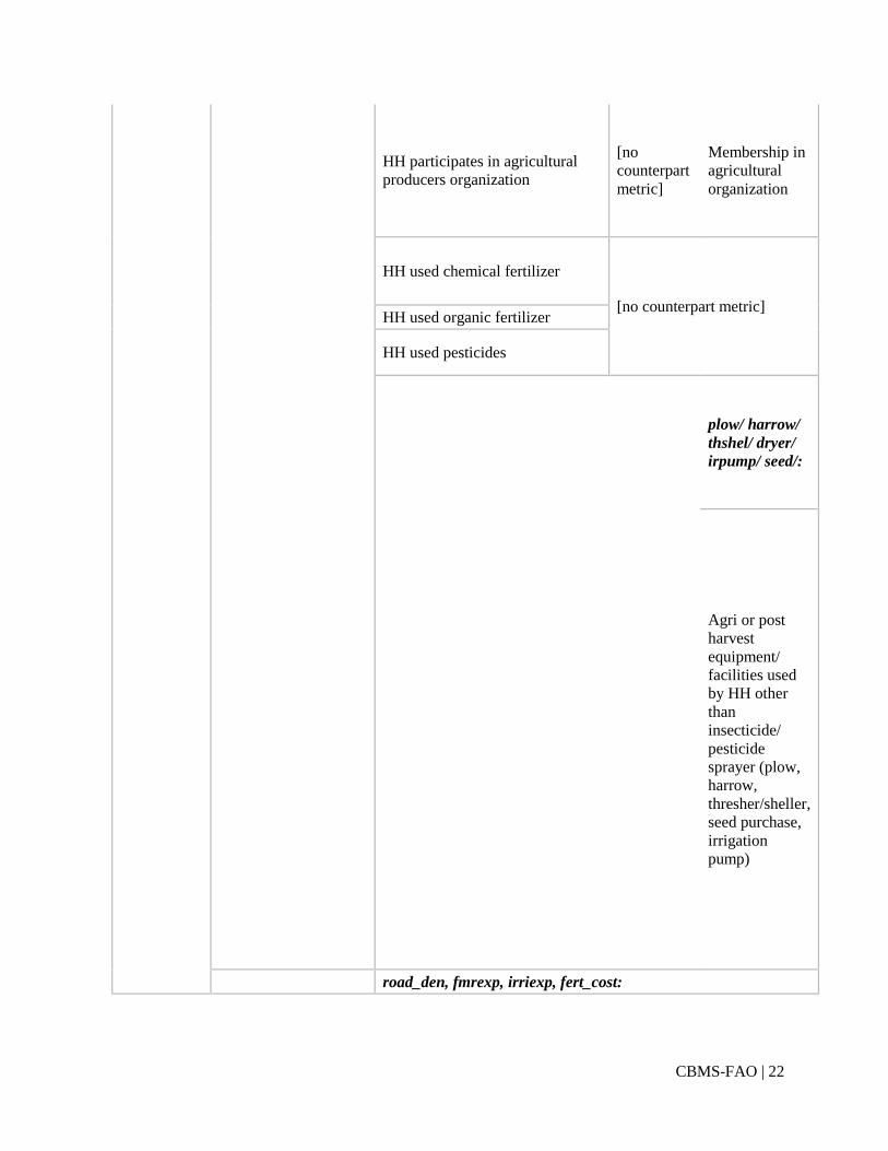
Data mapping

Identifying the variables for the model as executed in the FAO study is almost straightforward for the

national survey of the Philippines which is the FIES as well as for the CBMS data of local government units

(LGUs). Table 4 shows mapping of the variables (dependent, explanatory and instruments) used in the

FAO study with FIES and CBMS data.

Table 4. Data and variable mapping and initial variables

Model variable

Metrics or substitute metrics

FAO model FIES data CBMS data

Dependent

variable Food security

Value of food consumed per adult

equivalent

foodexp: malnutrition

Per capita

expenditure

on food

With

malnourished

children 0-5

years old

Explanatory

variables

Agricultural

productivity

Value of agri production per acre cropinc:

Income from crop farming

Characteristics of the

head of the household

Age of HH head age_yr:

Age of HH head

Years of education of HH head educlvl :

CBMS-FAO | 19

Categorized educational

attainment

Female Head fhead:

Female Head

Indigenous HH

[no

counterpart

metric]

ipindHH:

Indigenous HH

Access to migration

channels Access to HH migration network

migrnet: migrnet:

With

amount of

cash

receipts,

gifts, relief

and

assistance

from

abroad

With amount of

cash receipts,

gifts, relief and

assistance from

abroad

(remittance

from OFWs

combined with

other support

from abroad)

Characteristic of

household dwelling

Number of rooms in dwelling [no counterpart metric]

mshous:

HH with strong construction

materials of walls and roof

Access to information

and non-agri assets

HH has access to safe water sws:

HH has access to safe water

Number of radios owned nradio:

Number of radios owned

CBMS-FAO | 20

Number of TV sets owned ntv:

Number of TV sets owned

Communication

infrastructure

Time to nearest health facility

(min) [no counterpart metric]

tele:

With telephone / landline

Time to nearest primary school

(min) [no counterpart metric]

[no

counterpart

metric]

Household

transportation Number of bikes in HH

car:

With motorcycles/ vehicles

Availability of

farmland Agri land operated (imputed)

(as agricultural asset in

instruments)

Social infrastructure

Participation in community

organization

[no

counterpart

metric]

mworg:

HH members

who participate

in community

organization

HH received loan payloan: recloan:

CBMS-FAO | 21

Indicator

on HH

Cash loan

payments

Household

access to credit

programs

Social protection

Number of government programs

accessed

[no

counterpart

metric]

Number of NGO prgrams

accessed

[no

counterpart

metric]

privpind:

NGO prgrams

accessed

payprem:

Indicator

on HH

expenditure

on life

insurance

and

retirement

premiums

Illness shock

[no

counterpart

metric]

illshock:

At least one

member of HH

got sick

Instruments Climate variables Temperature (change)

drfyr, dseasonrf, dvolrf,

dtmin, dtmax:

Temperature, rainfall from

Philippine Atmospheric,

Geophysical and

Astronomical Services

Administration (PAGASA)

Agricultural Assets agriorg:

CBMS-FAO | 22

HH participates in agricultural

producers organization

[no

counterpart

metric]

Membership in

agricultural

organization

HH used chemical fertilizer

[no counterpart metric] HH used organic fertilizer

HH used pesticides

plow/ harrow/

thshel/ dryer/

irpump/ seed/:

Agri or post

harvest

equipment/

facilities used

by HH other

than

insecticide/

pesticide

sprayer (plow,

harrow,

thresher/sheller,

seed purchase,

irrigation

pump)

road_den, fmrexp, irriexp, fert_cost:

CBMS-FAO | 23

Agricultural

assistance/

infrastructure

Road density, expenditure on farm to market roads, expenditure

on irrigation, cost of fertilizer policy variables (Secondary data)

1 In the case of this study, agriculture production is potentially endogenous in explaining food consumption.

1 The first stage equation includes dummy for time (quarter) to control for the pooled time-series.

The variables in Table 4 will be the initial set of variables in estimating the models as discussed in the

following model scenarios.

Model scenarios

Consider the following model

food security = 𝑓

(

𝑎𝑔𝑟𝑖 𝑖𝑛𝑐𝑜𝑚𝑒, ℎℎ ℎ𝑒𝑎𝑑 𝑐ℎ𝑎𝑟𝑎𝑐𝑡𝑒𝑟𝑖𝑠𝑡𝑖𝑐𝑠,

𝑎𝑐𝑐𝑒𝑠𝑠 𝑡𝑜 𝑚𝑖𝑔𝑟𝑎𝑡𝑖𝑜𝑛 𝑐ℎ𝑎𝑛𝑛𝑒𝑙𝑠,

ℎ𝑜𝑢𝑠𝑒ℎ𝑜𝑙𝑑 𝑑𝑤𝑒𝑙𝑙𝑖𝑛𝑔, 𝑛𝑜𝑛 − 𝑎𝑔𝑟𝑖𝑐𝑢𝑙𝑡𝑢𝑟𝑎𝑙 𝑎𝑠𝑠𝑒𝑡𝑠,

𝑐𝑜𝑚𝑚𝑢𝑛𝑖𝑐𝑎𝑡𝑖𝑜𝑛 𝑖𝑛𝑓𝑟𝑎,

ℎ𝑜𝑢𝑠𝑒ℎ𝑜𝑙𝑑 𝑡𝑟𝑎𝑛𝑠𝑝𝑜𝑟𝑡, 𝑠𝑜𝑐𝑖𝑎𝑙 𝑖𝑛𝑓𝑟𝑎, 𝑠𝑜𝑐𝑖𝑎𝑙 𝑝𝑟𝑜𝑡𝑒𝑐𝑡𝑖𝑜𝑛)

+ 𝑢 (1)

agri income = 𝑓

(

[𝑐𝑙𝑖𝑚𝑎𝑡𝑜𝑙𝑜𝑔𝑦: 𝑟𝑎𝑖𝑛𝑓𝑎𝑙𝑙, 𝑠𝑒𝑎𝑠𝑜𝑛𝑎𝑙𝑖𝑡𝑦,

𝑣𝑜𝑙𝑎𝑡𝑖𝑙𝑖𝑡𝑦, 𝑡𝑒𝑚𝑝𝑒𝑟𝑎𝑡𝑢𝑟𝑒],

𝑎𝑔𝑟𝑖 𝑎𝑠𝑠𝑒𝑡𝑠, 𝑎𝑔𝑟𝑖 𝑎𝑠𝑠𝑖𝑠𝑡𝑎𝑛𝑐𝑒 𝑜𝑟

𝑖𝑛𝑓𝑟𝑎𝑠𝑡𝑟𝑢𝑐𝑡𝑢𝑟𝑒, 𝑒𝑡𝑐. ,[𝑠𝑒𝑐𝑜𝑛𝑑 𝑠𝑡𝑎𝑔𝑒 𝑣𝑎𝑟𝑖𝑎𝑏𝑙𝑒𝑠] )

+ 𝑣 (2)

where the dependent variable has finite mean and the explanatory variables can be continuous or categorical.

By assumption, the error terms u and v have zero mean and zero correlation with any of the explanatory

variables.

In the event that at least one of the explanatory variables, say agricultural productivity, is correlated with

the error term, estimates for the coefficients of the independent variables can be inconsistent2.

Instrumental variables (IV) method addresses this by introducing observable variable that is uncorrelated

with the error term but partially correlated with the endogenous variable.

Similar to FAO study of Karfakis, et al. (201), modeling using FIES dataset will work around the two-

stage least squares (2SLS) method in estimating the coefficients of the following model as analog to

equation (1).

2 In the case of this study, agriculture production is potentially endogenous in explaining food consumption.

CBMS-FAO | 24

food expenditure = 𝑓

(

𝑎𝑔𝑟𝑖 𝑖𝑛𝑐𝑜𝑚𝑒, ℎℎ ℎ𝑒𝑎𝑑 𝑐ℎ𝑎𝑟𝑎𝑐𝑡𝑒𝑟𝑖𝑠𝑡𝑖𝑐𝑠,

𝑎𝑐𝑐𝑒𝑠𝑠 𝑡𝑜 𝑚𝑖𝑔𝑟𝑎𝑡𝑖𝑜𝑛 𝑐ℎ𝑎𝑛𝑛𝑒𝑙𝑠,

ℎ𝑜𝑢𝑠𝑒ℎ𝑜𝑙𝑑 𝑑𝑤𝑒𝑙𝑙𝑖𝑛𝑔, 𝑛𝑜𝑛 − 𝑎𝑔𝑟𝑖𝑐𝑢𝑙𝑡𝑢𝑟𝑎𝑙 𝑎𝑠𝑠𝑒𝑡𝑠,

𝑐𝑜𝑚𝑚𝑢𝑛𝑖𝑐𝑎𝑡𝑖𝑜𝑛 𝑖𝑛𝑓𝑟𝑎,

ℎ𝑜𝑢𝑠𝑒ℎ𝑜𝑙𝑑 𝑡𝑟𝑎𝑛𝑠𝑝𝑜𝑟𝑡, 𝑠𝑜𝑐𝑖𝑎𝑙 𝑖𝑛𝑓𝑟𝑎, 𝑠𝑜𝑐𝑖𝑎𝑙 𝑝𝑟𝑜𝑡𝑒𝑐𝑡𝑖𝑜𝑛)

+ 𝑢 (3)

where the same function for agricultural income. On the other hand, IV probit regression will be

implemented on CBMS data with dependent variable malnutrition,3

Pr (malnutrition) = 𝑓

(

𝑎𝑔𝑟𝑖 𝑖𝑛𝑐𝑜𝑚𝑒, ℎℎ ℎ𝑒𝑎𝑑 𝑐ℎ𝑎𝑟𝑎𝑐𝑡𝑒𝑟𝑖𝑠𝑡𝑖𝑐𝑠,

𝑎𝑐𝑐𝑒𝑠𝑠 𝑡𝑜 𝑚𝑖𝑔𝑟𝑎𝑡𝑖𝑜𝑛 𝑐ℎ𝑎𝑛𝑛𝑒𝑙𝑠,

ℎ𝑜𝑢𝑠𝑒ℎ𝑜𝑙𝑑 𝑑𝑤𝑒𝑙𝑙𝑖𝑛𝑔, 𝑛𝑜𝑛 − 𝑎𝑔𝑟𝑖𝑐𝑢𝑙𝑡𝑢𝑟𝑎𝑙 𝑎𝑠𝑠𝑒𝑡𝑠,

𝑐𝑜𝑚𝑚𝑢𝑛𝑖𝑐𝑎𝑡𝑖𝑜𝑛 𝑖𝑛𝑓𝑟𝑎,

ℎ𝑜𝑢𝑠𝑒ℎ𝑜𝑙𝑑 𝑡𝑟𝑎𝑛𝑠𝑝𝑜𝑟𝑡, 𝑠𝑜𝑐𝑖𝑎𝑙 𝑖𝑛𝑓𝑟𝑎, 𝑠𝑜𝑐𝑖𝑎𝑙 𝑝𝑟𝑜𝑡𝑒𝑐𝑡𝑖𝑜𝑛)

+ 𝑢 (4)

This is operationalized by focusing on households engaged in crop farming and gardening. They are

approximately 30 percent of the original dataset, i.e. 12,000 households for FIES and 500,000 for CBMS.

In the case of CBMS malnutrition, the focus will be on households with members 0-5 years old or 40% of

the agricultural households, or about 220,000 households.

Climatology measures

Climate elements, in terms of rainfall and temperature, impact food insecurity through agricultural

production (farming income). To operationally represent them, three measures of rainfall and two

measures of temperature were explored: absolute level of rainfall, rainfall volatility, rainfall seasonality,

minimum temperature and maximum temperature. Absolute level of rainfall is a function of the (moving)

average of the monthly values of the climate variables, i.e.

𝑅𝐹̅̅ ̅̅ 𝑡 =1

12𝑡∑𝑅𝐹𝑖

12𝑡

𝑖=1

Given the average rainfall, the standard deviation can be represented by

𝑆𝐷𝑡 = √1

12𝑡 − 1∑(𝑅𝐹𝑖 − 𝑅𝐹̅̅ ̅̅ 𝑡)

2

12𝑡

𝑖=1

where 𝑅𝐹𝑖 represents the rainfall value at month i and t is the number of years. Now, volatility is the

3 The first stage equation includes dummy for time (quarter) to control for the pooled time-series.

CBMS-FAO | 25

coefficient of variation given the number of years

𝐶𝑉𝑡 =𝑆𝐷𝑡

𝑅𝐹̅̅ ̅̅ 𝑡

where 𝑆𝐷𝑡 is the standard deviation while the seasonality index takes on Walsh and Lawler’s (1981)

measure

𝑆𝐼𝑦 =1

𝑅𝐹̅̅ ̅̅ 1|𝑦∑|𝑅𝐹𝑖|𝑦 −

𝑅𝐹̅̅ ̅̅ 1|𝑦

12|

12

𝑖=1

That is, for a given year y, 𝑅𝐹̅̅ ̅̅ 1|𝑦 is the average for the year and 𝑅𝐹𝑖|𝑦 is the value of rainfall on the ith month.

The seasonality measure for a collection of years 𝑦 is the average of all seasonality indices across those

years,

𝑆𝐼𝑦 =1

𝑛(𝑦)∑ 𝑆𝐼𝑦

𝑦𝑛(𝑦)

𝑖=𝑦1

The seasonality index facilitates measurement of the variability of rainfall in terms of seasonality over the

year. Sumner, et al (2001) provides indicative classification based on 𝑆𝐼𝑦 as shown in Table 5.

Table 5. Rainfall seasonality based on 𝑺𝑰𝒚

<0.19 Precipitation spread throughout the year

0.20–0.39 Precipitation spread throughout the year, but with a definite wetter season

0.40–0.59 Rather seasonal with a short drier season

0.60–0.79 Seasonal

0.80–0.99 Markedly seasonal with a long dry season

1.00–1.19 Most precipitation in <3 months

>1.20 Extreme seasonality, with almost all precipitation in 1–2 months

Given the aforementioned formulas, the climate shocks are measured through change in each climate

variable for each year compared to long run average which is set as 1979-2006. These were computed

using the following:

1. Change in current year average rainfall to long run average in 1979-2006:

𝑑𝑅𝐹𝑦 = 100(𝑅𝐹̅̅ ̅̅ 1|𝑦

𝑅𝐹̅̅ ̅̅ 28|1979−2006− 1)

2. Change in current year rainfall seasonality relative to long run seasonality in 1979-2006:

CBMS-FAO | 26

𝑑𝑆𝐼𝑦 = 100 (𝑆𝐼𝑦

𝑆𝐼1979−2006− 1)

3. Change in current year rainfall volatility relative to long run volatility in 1979-2006:

𝑑𝐶𝑉𝑦 = 100(𝐶𝑉1|𝑦

𝐶𝑉28|1979−2006− 1)

4. Change in maximum/minimum temperature in current year compared to long run average in

1979-2006:

𝑑𝑇𝑀𝐴𝑋𝑦 = max𝑦(𝑇𝑀𝐴𝑋) −

1

28∑ max

𝑖(𝑇𝑀𝐴𝑋)

2006

𝑖=1979

𝑑𝑇𝑀𝐼𝑁𝑦 = min𝑦(𝑇𝑀𝐼𝑁) −

1

28∑ min

𝑖(𝑇𝑀𝐼𝑁)

2006

𝑖=1979

Where max𝑖(𝑇𝑀𝐴𝑋) and min

𝑖(𝑇𝑀𝐴𝑋) are maximum and minimum temperature at year i,

respectively.

Estimation

The final model specification varies according to the underlying trend in each dataset. Hence, the choice

of level or form of measurement is essential in coming up with the final model. Take, for example, the

climatology measures, including each of the climate variables without transformation is taken generally as

assuming that the relationship between income from agriculture and say change in rainfall is linear. In this

subsection, the objective is to establish the fact that the relationship is non-linear and interpretation of the

trend will be deferred until the specific datasets since there are other explanatory variables.

CBMS-FAO | 27

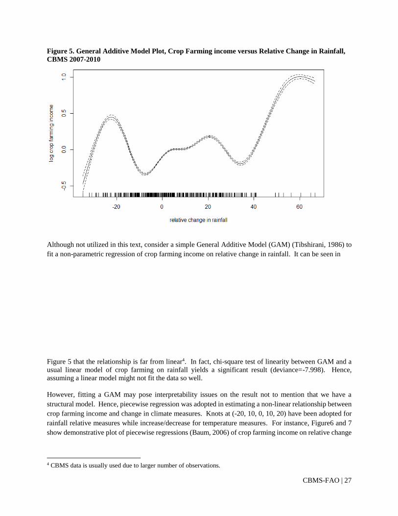
Figure 5. General Additive Model Plot, Crop Farming income versus Relative Change in Rainfall,

CBMS 2007-2010

Although not utilized in this text, consider a simple General Additive Model (GAM) (Tibshirani, 1986) to

fit a non-parametric regression of crop farming income on relative change in rainfall. It can be seen in

Figure 5 that the relationship is far from linear4. In fact, chi-square test of linearity between GAM and a

usual linear model of crop farming on rainfall yields a significant result (deviance=-7.998). Hence,

assuming a linear model might not fit the data so well.

However, fitting a GAM may pose interpretability issues on the result not to mention that we have a

structural model. Hence, piecewise regression was adopted in estimating a non-linear relationship between

crop farming income and change in climate measures. Knots at (-20, 10, 0, 10, 20) have been adopted for

rainfall relative measures while increase/decrease for temperature measures. For instance, Figure6 and 7

show demonstrative plot of piecewise regressions (Baum, 2006) of crop farming income on relative change

4 CBMS data is usually used due to larger number of observations.

CBMS-FAO | 28

in rainfall and temperature. Note that indeed the effects change locally. Furthermore, the choice of measure

consequently assumes jumps between the knots and the magnitude of jumps are significantly different.

Figure 6. Fitted values of regression without (left chart) and with spline dummy (right chart),

Change in Rainfall, CBMS 2007-2010

Note: F-test for equality of dummies significant

Figure 7. Fitted values of regression without (left) and with spline dummy (right), Change in TMIN,

CBMS 2007-2010

Note: F-test for equality of dummies significant

Another challenge on interpretability is collinearity between climate variables. For example, the three

measures of rainfall change are inherently correlated since they are first and second order measures of

rainfall (average and dispersion). This leads us to have four models for each of the dataset, which will be

discussed in the results.

Standard assumptions on the error terms are to be validated and tests for weak instrument, exogeneity and

overidentification are to be undertaken through the instrumental variable regression module in Stata (see

appendix). It is inevitable in some cases to encounter violation of assumptions but are taken as it is either

due to data issues or due to interpretability. For instance, overidentification may be a problem in FIES

dataset (Sargan’s statistic) which might be due to the number of instruments. Outliers can be menacing in

CBMS-FAO | 29

this case and have been identified using Cook’s distances. Many of them are ignored in order to balance

the regions, provinces and municipalities to be retained which is an integral element of the objectives in

this study.

Given the estimation procedure, this paper presents the eight models—four independent climate variable

models for each data set. The results will be discussed in the succeeding section.

5. Results

Having different set of samples with different set of time periods may show different trends in the effects

of climate shocks as well as its covariates. It is important however, to depict the expected change in climate

variables in the future to facilitate interpretation of the manifestation of changes in climate.

Changes in climate

Table 6 shows the general changes in the measures of climate change used in this study. It can be noted

that, overall, all of the climate variables will increase in the future except for the rainfall seasonality.

However, only the maximum temperature and minimum temperature will have a significant change, at 37

percent and 47 percent respectively. A closer inspection across provinces will show that there are varying

changes in the inspected climate variables.

Table 6. Change in climate variables 1979-2006 and 2011-2040, Philippines

Climate variable Mean

Change 1979-2010 2011-2040

Mean cumulative annual rainfall 2693.2 2827.7 5.0%

Mean rainfall seasonality 0.50 0.50 0.3%

Volatility of rainfall 0.65 0.67 3.7%

Mean maximum annual temperature

(degree C) 32.10 32.47 37.0%

Mean minimum annual temperature

(degree C) 20.16 20.63 47.0%

Figure shows the provinces covered by CBMS in comparison with the country average. It shows that

although Philippines is expected to have increased rainfall in the future, CBMS coverage includes some

provinces that decreased in rainfall. Similarly, it can be seen in Figure9 that still, many provinces in the

CBMS dataset will likely experience lower increase in minimum temperature than the country average.

CBMS-FAO | 30

Figure 8. Difference in rainfall (1979-2006, 2011-2040)

Source: Provincial estimates provided by PAGASA-AMICAF Project Team based on the MPEH5 estimates using the Global

Climate Model

Figure 9. Relative differences in minimum (left) and maximum (right) temperature (1979-2006,

2011-2040)

Source: Provincial estimates provided by PAGASA-AMICAF Project Team based on the MPEH5 estimates using the Global

Climate Model

-5 0 5 10 15

Surigao Del Sur

Sarangani

Surigao Del Norte

Northern Samar

Agusan Del Norte

Camiguin

Camarines Sur

Batanes

Philippines

Kalinga

Romblon

Tarlac

Occidental Mindoro

Oriental Mindoro

Marinduque

Batangas

Benguet

0 1 2 3 4

Camiguin

Surigao Del Sur

Romblon

Surigao Del Norte

Northern Samar

Oriental Mindoro

Kalinga

Agusan Del Norte

Batanes

Tarlac

Philippines

Marinduque

Camarines Sur

Sarangani

Batangas

Occidental Mindoro

Benguet

0 0.5 1 1.5

Surigao Del Norte

Surigao Del Sur

Northern Samar

Sarangani

Marinduque

Kalinga

Agusan Del Norte

Occidental Mindoro

Benguet

Philippines

Tarlac

Camarines Sur

Romblon

Batangas

Camiguin

Oriental Mindoro

Batanes

CBMS-FAO | 31

Different data, different results

These findings serve as guidance on the expected differences in trends in the national and CBMS results.

Hence, although general trends of effects of climate on crop farming income and eventually on vulnerability

to food insecurity maybe expected to be consistent, there is an expected disparity in trends as well in some

of the factors that will be exhibited in later parts of this paper. It is worth mentioning that 2009 marks the

year of Ondoy and higher rainfall can be expected in this year compared to other years. This is also coupled

with differences in time periods (2009 and 2007-2010), differences in scope (national sample and censuses

from 16 provinces), and differences in food insecurity measures (value of food consumption and

malnutrition).

A. Family Income and Expenditure Survey 2009

Effect of climate variables on income from crop farming and gardening and vulnerability

Using the data of Family Income and Expenditure Survey for 2009, the different measures of rainfall and

temperature have varying effects on crop farming and income and subsequently on food insecurity. Table

7 shows the effect of percent change in level of rainfall, seasonality, volatility, decrease in minimum

temperature and increase in maximum tempearture on income from crop farming and gardening.

Table 7. Effect of different climate variables on income from crop farming and gardening, FIES

2009

Categories

ln of income from farming and gardening

Rainfall Seasonality Volatility Temperature

Coef. Std.

Err. Coef.

Std.

Err. Coef.

Std.

Err. Coef.

Std.

Err.

<-20%

0.017**

* 0.001

0.014**

* 0.001

<=20% - <-10% -0.072 0.086 -0.016 0.015

-10% - <0% 0.166**

* 0.015

0.047**

* 0.011 -0.014* 0.007

0%-<10% 0.031**

* 0.012 -0.026** 0.012

0.043**

* 0.012

10% - <20% -0.015** 0.007

0.053**

* 0.014 -0.209** 0.098

>=20%

-

0.005**

* 0.001 -0.026. 0.017 0.007 0.007

Dummies

<-20% -0.058 0.530

0.932**

* 0.262

<=2-0% - <-10% -1.992* 1.195 -0.215 0.330

-10% - <0% 0.866**

* 0.088 -0.614 0.533 0.304 0.262

0%-<10%

-

0.261**

* 0.093 0.744 0.532 -0.038 0.266

10% - <20% -0.094

0.119

-

1.651**

* 0.566 3.328** 1.536

Decrease in min temp

0.990**

* 0.338

CBMS-FAO | 32

Increase in max temp

-

0.249**

* 0.064

Dummies

Decrease in min temp

0.728**

* 0.078

Increase in max temp 0.028 0.029

ln per capita food expenditure

ln of income from farming and

gardening

0.141**

* 0.014

0.131**

* 0.014

0.167**

* 0.016

0.169**

* 0.016

Sig. codes *** 2.5% ** 5% * 10% . 15% Percent change in rainfall

Change in level of rainfall expressed in terms of percent change in current level of rainfall relative to 1979-

2006 average rainfall has varying effect on income from crop farming and gardening as well as on food

insecurity. Small relative changes in level of rainfall increase income from crop farming and gardening and

expectedly extreme increase in level of rainfall (i.e. more than 10%) decreases income from crop farming

and gardening. In particular, decrease in rainfall, translated to greater than zero to 10 percent relative change,

tends to significantly increase income. Similarly, income increases when level of rainfall increases up to

less than 10 percent. However, significant decrease in income is observed when percent change in rainfall

is equal or more than 10 percent.

Percent change in seasonality

Different ranges of percent change in seasonality of rainfall give mixed impact on income from crop

farming and gardening. For more than 20 percent decrease in seasonality of rainfall, income significantly

increases. The same trend is true when the decrease in seasonality is more than zero to 10 percent and more

than 10 percent to less than 20 percent. When percent change in seasonality falls between -20 percent to -

10 percent and 0 percent to 10 percent or more than 20 percent, income will decrease. Generally, crop

farming and gardening income increases when rainfall is less seasonal. However, more seasonal rainfall

have mixed effects on crop farming income.

Percent change in volatility

Mixed effects are observed when there are relatively small changes in rainfall volatility. Decrease in

volatilty translated to 0-10 percent change will significantly reduce income from crop farming and

gardening. The same trend is also observed when volatility increases between 10 to less than 20 percent.

Increase in volatility between 0-10 percent significantly increases income. However, extreme negative

change in rainfall volatility (e.i., more than 20%) increases crop farming income.

Temperature

Minimum and maximum temperatures have opposite effects on crop farming and gardening income.

Decrease in 2009 minimum temperature relative to the 1979-2006 average minimum temperature is

significant and positive with regard to income from crop farming and gardening. On the other hand, increase

in maximum temperature affects income negatively and significantly. These effects imply that hotter

temperature means lower crop farming income while colder temperature means higher farming income.

CBMS-FAO | 33

Effects of crop farming income on food insecurity as measured by per capita food expenditure are consistent

across the models. Increase in crop farming and income will lead to increased per capita food expenditure

hence will reduce vulnerability of population to food insecurity.

Covariates

Demographic characteristics

Across all climate shocks, age of the head of the family is negatively correlated with income from crop

farming and gardening. Female headed family is also negatively associated with income. Educational

attainment of the head of the family generally has negative effect on income which indicates that lower

educational attainment is associated with higher reduction in income. Age, sex and educational attainment

of the head of the family with regard to food expenditure is positive and significant. A year added on age

of the head of the family increases food expenditure by .006. In addition, as level of educational attainment

increases, food expenditure also increases..

Assets

Proxy variables of non-agricutural assets such as strong materials of walls and roof and access to safe water

have different effect on income. Dwelling unit with strong walls and roof has positive effect on income,

however families with access to safe water supply have negative effect. With regard to food expenditure,

both have significant positive effect. In particular, there is about 5 percent increase in food expenditure

among those families with strong materials of walls and roof as compared to those made from

light/makeshift materials. Similarly, expenditure on food is higher by 6 percent among families with access

to safe water.

Family’s access to information as approximated by ownership of radio and TV significantly influences

income from crop farming and gardening as well as food expenditure. Income of families with radio is 13-

15 percent higher than the income of families without radio. Families who own a TV have higher income

of about 6-9 percent as compared to those families who do not own a TV. Both the ownership of radio and

TV increase food expenditure by 2 percent and 9 percent, respectively.

Ownership of car and motorcycle as proxies to family’s access to transportation is significantly associated

with both income and food expenditure. Ownership of car tends to increase income by almost 51-54 percent

and thus increases spending on food by 15-17 percent. Onwership of motorcycle also gives higher income

by 16-20 percent therefore food spending increases by 6-7 percent.

Infrastructure

Included in the models are several variables that are proxies of communication infrastructure (ownership

of telephone), financial infrastructure (cash loan payments) and social welfare infrastructure (expenditure

on insurance and premiums). These variables, however, tend to have different effect on income. For

instance, both ownership of telephone and payments to loan affect income positively while expenditure

on social welfare affects income negatively. With respect to spending on food, both ownership of telephone

and expenditure on social welfare are associated with higher spending on food while expenditure on loan

decreases spending on food but not significant.

CBMS-FAO | 34

Policy Variables

Both policy variables included in the models are significantly associated with income from crop farming

and gardening. Across all models, a unit increase in spending on farm-to-market roads will increase income

by 0.1 percent. Also, a unit increase in spending on irrigation for palay significantly increases income by

2-3 percent. These results imply that policies directed toward agriculture infrastructures will provide

farmers higher income and as a result will increase food expenditure that will lead to reduce food insecurity.

Location

Location of familes as either in rural or urban areas significantly affect income from crop farming and

gardening. For instance, income from crop farming and gardening of those families living in rural area is

higher than those families in urban areas at about 10-13 percent.

Effects of climate shocks on the likelihood of being food insecure

Level of rainfall and temperature as climate shocks have opposite effects on food insecurity in the future.

At the national level, proportion of food insecure families due to temperature shock will increase by 0.43

percent while relative change in level of rainfall will reduce proportion of food insecure families in the

future by 0.18 percent.Variations on the effects of climate shocks are more pronounced at the regional level

as shown in table 8. For rainfall shock, there are regions that are negatively affected but there are also

regions that are positively affected. In particular, Caraga region will experience increase in proportion of

familes who are food insecure in the future. However, nine regions namely Ilocos, Cagayan Valley, Bicol,

Central and Eastern Visayas, Zamboanga, Northern Mindanao, Davao and ARMM will benefit from the

change in rainfall and in turn lower proportion of food insecure families (Map 1). On the other hand,

temperature shock will negatively affect almost all regions leading to increase in food insecure families as

shown in Map 2.

Table 8. Predicted and projected vulnerability, rainfall and temperature model, FIES 2009

Region

Rainfall Temperature

Predicted

2009

Projected (2011-

2040)

Predicted 2009 Projected (2011-

2040)

Philippines 13.45% 13.27% 13.45% 13.88%

I - Ilocos Region 3.80% 3.80% 3.80% 4.05%

II - Cagayan Valley 1.68% 1.57% 1.57% 2.13%

III - Central Luzon 1.90% 1.90% 1.90% 2.47%

IVA - CALABARZON 5.52% 5.52% 5.52% 5.71%

V - Bicol Region 11.31% 10.89% 11.31% 12.15%

VI - Western Visayas 8.65% 8.65% 8.65% 9.16%

VII - Central Visayas 27.94% 27.33% 28.06% 28.43%

VIII - Eastern Visayas 17.40% 17.30% 17.30% 17.82%

IX - Zamboanga Peninsula 29.33% 29.07% 29.33% 29.33%

X - Northern Mindanao 21.48% 21.19% 21.34% 21.77%

CBMS-FAO | 35

XI – Davao 17.70% 17.33% 17.70% 17.94%

XII - SOCCSKSARGEN 14.74% 14.74% 14.74% 14.74%

CAR 7.27% 7.27% 7.27% 8.55%

ARMM 8.74% 8.21% 8.95% 8.95%

XII – Caraga 22.19% 22.49% 22.19% 22.64%

IVB – MIMAROPA 14.53% 14.29% 14.53% 15.02% Source of basic data: Philippine Statistics Authority – Food and Income Expenditure Survey 2009

Source of basic data: Philippine Statistics Authority – Food and Income Expenditure Survey

Chronic and transient food insecurity due to rainfall and temperature shock

At least 8 in every 10 families who are food secure today will still remain food secure in the future, given

rainfall and temperature as climate shocks. Proportion of families who are chronically food insecure due to

changes in level of rainfall and temperature are about 13.2 and 13.5 percent, respectively. Furthermore,

transitory food insecure due to rainfall is about 0.2 percent and slightly higher for temperature shock at 0.4

percent. Across the regions, Zamboanga region has the highest proportion of families who are chronically

food insecure (both in rainfall level and temperature) with almost 30 percent of the families in the region

experiencing this. Proportion of never food insecure families is highest in Cagayan Valley region where 9

in every 10 families did not experience and will not experience food insecurity in the future. On the other

hand, Central Visayas and Davao regions will have the highest proportion of families who are transitory

food insecure given level of rainfall as the climate shock. It is worth noting that more than 1 percent of the

families in CAR region are transitory food insecure due changes in temperature in the future.

Map 1. Change in predicted and projected

vulnerability, rainfall model, FIES 2009

Map 2. Change in predicted and projected

vulnerability, temperature model, FIES

2009

CBMS-FAO | 36

Table 9. Characteristics of families in chronic and transient food insecurity by region , FIES 2009

Province

Rainfall Temperature

Never food

insecure

Transitory

food

insecure

Chronically

food

insecure

Never food

insecure

Transitory

food

insecure

Chronically

food insecure

Philippines 86.52% 0.24% 13.24% 86.12% 0.43%

13.45%

I - Ilocos Region 96.20% 0.00% 3.80% 95.95% 0.25% 3.80%

II - Cagayan Valley 98.32% 0.11% 1.57% 97.87% 0.56% 1.57%

III - Central Luzon 98.10% 0.00% 1.90% 97.53% 0.57% 1.90%

IVA - CALABARZON 94.48% 0.00% 5.52% 94.29% 0.19% 5.52%

V - Bicol Region 88.69% 0.42% 10.89% 87.85% 0.84% 11.31%

VI - Western Visayas 91.35% 0.00% 8.65% 90.84% 0.52% 8.65%

VII - Central Visayas 72.06% 0.61% 27.33% 71.57% 0.37% 28.06%

VIII - Eastern Visayas 82.49% 0.31% 17.19% 82.18% 0.52% 17.30%

IX - Zamboanga

Peninsula 70.67% 0.27% 29.07% 70.67% 0.00% 29.33%

X - Northern Mindanao 78.52% 0.29% 21.19% 78.23% 0.44% 21.34%

XI - Davao 82.18% 0.61% 17.21% 82.06% 0.24% 17.70%

XII - SOCCSKSARGEN 85.26% 0.00% 14.74% 85.26% 0.00% 14.74%

CAR 92.73% 0.00% 7.27% 91.45% 1.27% 7.27%

ARMM 91.26% 0.53% 8.21% 91.05% 0.00% 8.95%

XII - Caraga 77.51% 0.30% 22.19% 77.36% 0.45% 22.19%

IVB - MIMAROPA 85.47% 0.25% 14.29% 84.98% 0.49% 14.53%

Source of basic data: Philippine Statistics Authority – Food and Income Expenditure Survey

Characteristics of vulnerable families

Differences on the characteristics of families among the never food insecure, transient food insecure and

chronically food insecure are also evident as shown in table 10. Families who are chronically food insecure

have relatively higher dependence on crop farming and gardening. However, it is worth noting that

transitory food insecure families affected by rainfall shock have relatively higher dependence on crop

farming and gardening income at about 40 percent. Food insecurity is likely to be experienced by families

with younger heads. Table 10 shows that average age of head among never food insecure families is higher

than those families who are transitory food insecure and permanently food insecure. Families with higher

household size have higher tendency to be food insecure. For instance, transitory food insecure and

permanently food insecure families have higher household size as compared to those permanently food

secure families. Lower educational attainment of the head of the family is also associated with food

insecurity. Dwelling unit with strong materials of walls and roof lessens the tendency of being food insecure.

CBMS-FAO | 37

Permanently food secure families have the highest proportion with strong walls and roof among the three

groups. Families with more assets such as TV, radio, telephone, car, and motorcycle are more likely to be

food secure. Access to social welfare such as insurance/retirement and access to credit lessen the tendency

of being food insecure.

Table 10. Characteristics of chronic and transient food insecure families, FIES 2009

Characteristic Rainfall Temperature

All Never food

insecure

Transitory

food

insecure

Chronically

food insecure

Never

food

insecure

Transitory

food

insecure

Chronically

food

insecure

Share of crop farming

income to total income 35.85% 35.46% 41.37% 38.35% 35.46% 33.36% 38.43%

Female headed 11.82% 4.66% 6.66% 6.61% 12.50% 7.41% 7.57%

Age of head 51.6 52.3 50.7 46.9 52.4 47.4 46.9

Family size 4.9 12.5 6.5 7.5 4.7 6.6 6.6

With strong house 61.37% 66.29% 25.81% 29.92% 66.32% 50.00% 30.03%

With radio 51.35% 54.04% 45.16% 33.91% 54.08% 46.30% 34.08%

With telephone 53.00% 58.13% 22.58% 20.08% 58.23% 35.19% 20.12%

With tv set 54.60% 60.44% 25.81% 16.98% 60.56% 33.33% 17.13%

With car 4.23% 4.89% - - 4.90% 1.85% -

With motorcycle 15.97% 18.13% 3.23% 2.09% 18.18% 5.56% 2.17%

Urbanity(rural) 84.99% 83.97% 87.10% 91.60% 83.95% 87.04% 91.55%

No grade 6.04% 5.17% 12.90% 11.62% 5.17% 5.56% 11.67%

Elementary level 33.16% 30.60% 51.61% 49.52% 30.61% 29.63% 49.62%

Elementary graduate 24.35% 24.67% 6.45% 22.59% 24.61% 33.33% 22.40%

High school level 11.64% 12.13% 16.13% 8.40% 12.15% 11.11% 8.45%

High school graduate 14.82% 16.11% 12.90% 6.38% 16.11% 18.52% 6.39%

College level 6.13% 6.88% - 1.37% 6.90% 1.85% 1.35%

College and post

graduate 3.87% 4.45% - 0.12% 4.44% - 0.12%

With remittance 19.04% 21.38% - 4.05% 21.45% 7.41% 3.99%

With safe water 69.32% 72.43% 35.48% 49.58% 72.43% 72.22% 49.27%

With cash loan

payments

25.36%

27.03% 19.35% 14.54%

27.05% 25.93% 14.49%

With expenditure on

insurance and

retirement

14.77% 16.80% - 1.79% 16.87% - 1.76%

Source of basic data: Philippine Statistics Authority – Food and Income Expenditure Survey

Policy Options

CBMS-FAO | 38

Based on the models, projected changes in temperature will lead to about 60% percent decrease in crop

farming income. Such impact on income will definetly put farmers at risk in terms of food security. This

impact, however, can be mitigated by policy interventions. Using our model, policy interventions can be in

the form of increased expenditures on agricultural infrastructure such as farm to market roads and irrigation

for palay (Figure 10). At the family level, increase in level of education of head of the family, ownership

of radio and access to remittances can also be usedto mitigate the negative effects of changes in temperature

(Figure 11).

Figure 10. Increasing expenditure on farm-to-market road and irrigation of palay at current value

of temperature, FIES 2009

Figure 11. Increasing ownership of asset, and access to remittance and enhancing education at

current value of temperature, FIES 2009

B. CBMS 2007-2010

Climate shocks

Models of food insecurity using CBMS 2007-2010 data suggest the expected general trend that higher

rainfall or hotter temperatures means lower crop farming income. Furthermore, small relative changes in

rainfall effect increase in crop farming and gardening although in different pace. It is notable, however,

that higher increase in rainfall still means lower crop farming income. On the other hand, seasonality and

volatility have varied effects such that small changes have positive effects on crop farming income. Finally,

CBMS-FAO | 39

temperature model suggests that increase in minimum temperature increases crop farming income to some

extent while maximum temperature decreases income from farming and gardening to some extent as well.

This means that temperature must not be too cold (too low minimum temperature) and must not be too hot

(too high maximum temperature).

Table 11. Effect of different climate shocks on income from crop farming and gardening, CBMS

2007-2010

Effect on

Malnutrition model

Income from crop farming (log)

-0.248*** -0.258*** -0.256*** -0.253***

Climate Variables Rainfall Rainfall

seasonality

Rainfall volatity

Temperature

Coef. Robust

SE

Coef. Robust

SE

Coef. Robust

SE

Coef. Robust

SE

Percent change

<=-20% -0.07*** 0.006 0.003*** 0.001 0.02*** 0.001

>-20% - <=-10% 0.03*** 0.004 0.02*** 0.005 0.02*** 0.002

>-10% - <=0% 0.03*** 0.004 -0.003 0.003 0.01*** 0.002

>0% - <=10% 0.01*** 0.004 0.001 0.004 0.03*** 0.003

>10% - <=20% 0.03*** 0.003 0.003 0.004 0.005 0.004

>20% 0.01*** 0.001 0.01*** 0.001 0.01*** 0.003

Percent change

intercept

<=-20% base

base

base

>-20% - <=-10% 1.70*** 0.157 0.23*** 0.069 -0.16*** 0.042

>-10% - <=0% 1.52*** 0.148 0.02 0.035 -0.37*** 0.032

>0% - <=10% 1.57*** 0.146 0.02 0.036 -0.71*** 0.036

>10% - <=20% 1.32*** 0.149 0.06 0.067 -0.53*** 0.068

>20% 1.42*** 0.151 -0.08* 0.045 -0.74*** 0.081

Change in

temperatures

Change in minimum

temperature

0.64*** 0.044

Decrease in minimum

temperature (dummy)

-0.33*** 0.049

Change in maximum

temperature

-0.09*** 0.021

Increase in maximum

temp (dummy)

0.09*** 0.027

Sig. codes *** 2.5% ** 5% * 10% . 15%

Change in rainfall

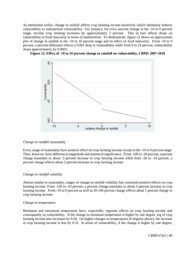
CBMS-FAO | 40

As mentioned earlier, change in rainfall affects crop farming income positively which ultimately reduces

vulnerability to malnutrition vulnerability. For instance, for every percent change in the -10 to 0 percent

range, income crop farming increases by approximately 3 percent. This in turn affects drops on

vulnerability to food insecurity in terms of malnutrition. To demonstrate, figure 12 shows an approximate

plot of change in rainfall in the -10 to 10 percent range and its effect on food insecurity. From -10 to 0

percent, a percent difference effects a 0.001 drop in vulnerability while from 0 to 10 percent, vulnerability

drops approximately by 0.0003.

Figure 12. Effect of -10 to 10 percent change in rainfall on vulnerability, CBMS 2007-2010

Change in rainfall seasonality

Every range of seasonality have positive effect on crop farming income except in the -10 to 0 percent range.

They, however, have different in magnitude and statistical significance. From -100 to -20 percent, a percent

change translates to about .3 percent increase in crop farming income while from -20 to -10 percent, a

percent change effects about 2 percent increase in crop farming income.

Change in rainfall volatility

Almost similar to seasonality, ranges of change in rainfall volatility has consistent positive effects on crop

farming income. From -100 to -10 percent, a percent change translates to about 2 percent increase in crop

farming income. From -10 to 0 percent as well as 20-100 percent change effects about 1 percent change in

crop farming income.

Change in temperature

Minimum and maximum temperature have, expectedly, opposite effects on crop farming income and

consequently on vulnerability. If the change in minimum temperature is higher by one degree, log of crop

farming income also increases by 0.64. On higher changes in temperatures (0 degrees above), the increase

in crop farming income is less by 0.33. In terms of vulnerability, if the change is higher by one degree,

CBMS-FAO | 41

there is approximately 0.02 reduction in vulnerability (see Figure 13). This reduction becomes slower in

higher positive changes in temperature, about 0.01.

Changes in maximum temperature demonstrates effects contrary to minimum. A degree higher change in

maximum temperature effects about 0.02 drop in log crop farming income. On higher changes in maximum

temperatures (0 degrees above), the drop in crop farming income is less by .01. These effects in turn

translates to approximately 0.002 increase in vulnerability, although the rate becomes slower by 0.002 in

higher changes.

Figure 13. Effect of change in minimum and maximum temperature on vulnerability, CBMS 2007-

2010

Covariates

Demographic characteristics

Age of the household head is consistently associated with lower probability of being malnourished across

all climate shocks. In addition female-headed households are less likely to have malnourished children.

On the other hand, households with indigenous member are more likely to have malnourished children as

well as those who have experienced illness in their households. Higher educational attainment of the

household head appear to reduce probability of malnourished children.

Household assets and infrastructure

Ownership of assets and access to infrastructure have mitigating effects on vulnerability to food insecurity

in terms of malnutrition. Those with safe water are less likely to have malnourished children compared to

those without safe water. Access to communication such as cellphone and telephone also reduces the

likelihood of having malnourished children. This is also similar with those who have access to media and

information such as radio. On the other hand, access to government programs is likely associated with

malnutrition as well as higher prices of food.

Policy Variables

Agricultural assets shows a robust effect on agricultural income and in turn on food insecurity. For instance

those with agricultural organization, thresher, dryer or irrigation pump will likely have more income on

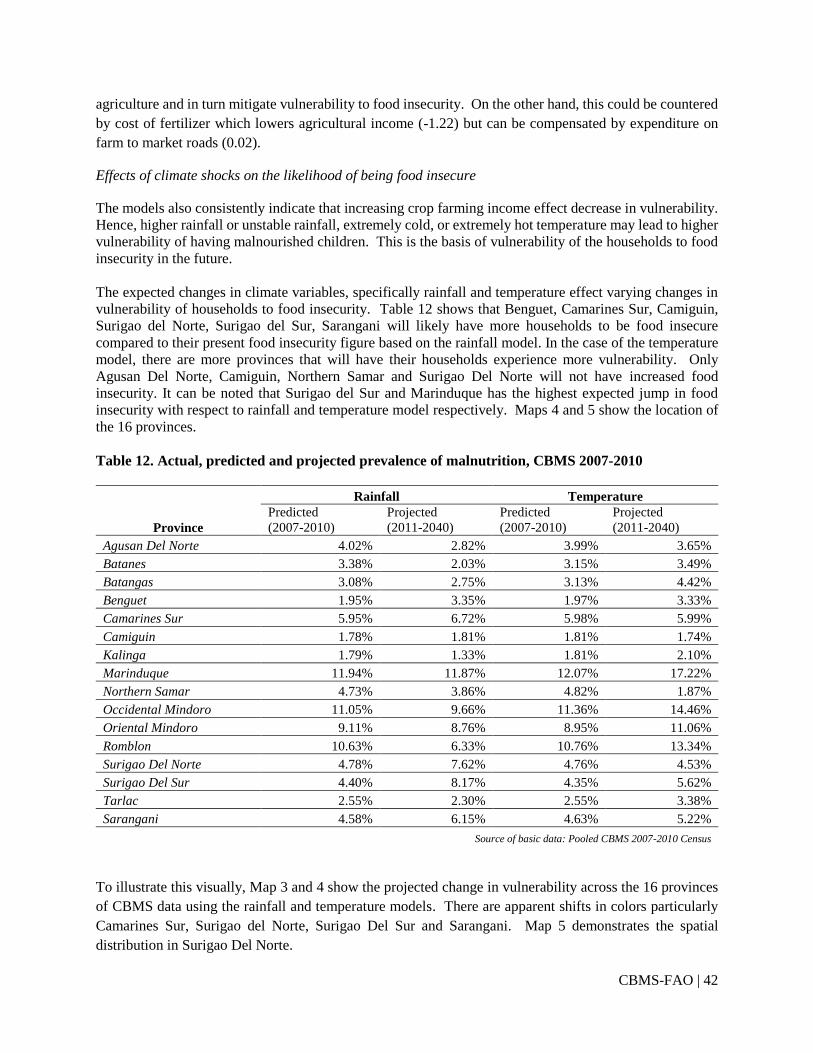
CBMS-FAO | 42

agriculture and in turn mitigate vulnerability to food insecurity. On the other hand, this could be countered

by cost of fertilizer which lowers agricultural income (-1.22) but can be compensated by expenditure on

farm to market roads (0.02).

Effects of climate shocks on the likelihood of being food insecure

The models also consistently indicate that increasing crop farming income effect decrease in vulnerability.

Hence, higher rainfall or unstable rainfall, extremely cold, or extremely hot temperature may lead to higher

vulnerability of having malnourished children. This is the basis of vulnerability of the households to food

insecurity in the future.

The expected changes in climate variables, specifically rainfall and temperature effect varying changes in

vulnerability of households to food insecurity. Table 12 shows that Benguet, Camarines Sur, Camiguin,

Surigao del Norte, Surigao del Sur, Sarangani will likely have more households to be food insecure

compared to their present food insecurity figure based on the rainfall model. In the case of the temperature

model, there are more provinces that will have their households experience more vulnerability. Only

Agusan Del Norte, Camiguin, Northern Samar and Surigao Del Norte will not have increased food

insecurity. It can be noted that Surigao del Sur and Marinduque has the highest expected jump in food

insecurity with respect to rainfall and temperature model respectively. Maps 4 and 5 show the location of

the 16 provinces.

Table 12. Actual, predicted and projected prevalence of malnutrition, CBMS 2007-2010

Province

Rainfall Temperature

Predicted

(2007-2010)

Projected

(2011-2040)

Predicted

(2007-2010)

Projected

(2011-2040)

Agusan Del Norte 4.02% 2.82% 3.99% 3.65%

Batanes 3.38% 2.03% 3.15% 3.49%

Batangas 3.08% 2.75% 3.13% 4.42%

Benguet 1.95% 3.35% 1.97% 3.33%

Camarines Sur 5.95% 6.72% 5.98% 5.99%

Camiguin 1.78% 1.81% 1.81% 1.74%

Kalinga 1.79% 1.33% 1.81% 2.10%

Marinduque 11.94% 11.87% 12.07% 17.22%

Northern Samar 4.73% 3.86% 4.82% 1.87%

Occidental Mindoro 11.05% 9.66% 11.36% 14.46%

Oriental Mindoro 9.11% 8.76% 8.95% 11.06%

Romblon 10.63% 6.33% 10.76% 13.34%

Surigao Del Norte 4.78% 7.62% 4.76% 4.53%

Surigao Del Sur 4.40% 8.17% 4.35% 5.62%

Tarlac 2.55% 2.30% 2.55% 3.38%

Sarangani 4.58% 6.15% 4.63% 5.22%

Source of basic data: Pooled CBMS 2007-2010 Census

To illustrate this visually, Map 3 and 4 show the projected change in vulnerability across the 16 provinces

of CBMS data using the rainfall and temperature models. There are apparent shifts in colors particularly

Camarines Sur, Surigao del Norte, Surigao Del Sur and Sarangani. Map 5 demonstrates the spatial

distribution in Surigao Del Norte.

CBMS-FAO | 43

Map 3. Predicted (left) and projected (right) vulnerability, rainfall model, CBMS 2007-2010

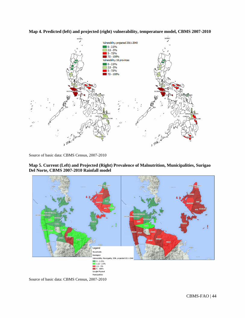
CBMS-FAO | 44

Map 4. Predicted (left) and projected (right) vulnerability, temperature model, CBMS 2007-2010

Source of basic data: CBMS Census, 2007-2010

Map 5. Current (Left) and Projected (Right) Prevalence of Malnutrition, Municipalities, Surigao

Del Norte, CBMS 2007-2010 Rainfall model

Source of basic data: CBMS Census, 2007-2010

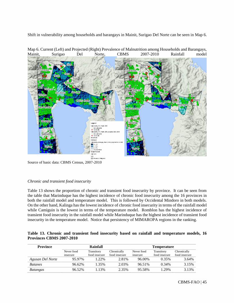
CBMS-FAO | 45

Shift in vulnerability among households and barangays in Mainit, Surigao Del Norte can be seen in Map 6.

Map 6. Current (Left) and Projected (Right) Prevalence of Malnutrition among Households and Barangays,

Mainit, Surigao Del Norte, CBMS 2007-2010 Rainfall model

Source of basic data: CBMS Census, 2007-2010

Chronic and transient food insecurity

Table 13 shows the proportion of chronic and transient food insecurity by province. It can be seen from

the table that Marinduque has the highest incidence of chronic food insecurity among the 16 provinces in

both the rainfall model and temperature model. This is followed by Occidental Mindoro in both models.

On the other hand, Kalinga has the lowest incidence of chronic food insecurity in terms of the rainfall model

while Camiguin is the lowest in terms of the temperature model. Romblon has the highest incidence of

transient food insecurity in the rainfall model while Marinduque has the highest incidence of transient food

insecurity in the temperature model. Notice that persistency of MIMAROPA regions in the ranking.

Table 13. Chronic and transient food insecurity based on rainfall and temperature models, 16

Provinces CBMS 2007-2010

Province Rainfall Temperature

Never food

insecure

Transitory

food insecure

Chronically

food insecure

Never food

insecure

Transitory

food insecure

Chronically

food insecure

Agusan Del Norte 95.97% 1.22% 2.81% 96.00% 0.35% 3.64%

Batanes 96.62% 1.35% 2.03% 96.51% 0.34% 3.15%

Batangas 96.52% 1.13% 2.35% 95.58% 1.29% 3.13%

CBMS-FAO | 46

Benguet 96.16% 2.39% 1.46% 96.65% 1.40% 1.95%

Camarines Sur 93.11% 1.12% 5.77% 93.71% 0.61% 5.68%

Camiguin 98.03% 0.34% 1.63% 98. 15% 0.15% 1.70%

Kalinga 98.12% 0.64% 1.24% 97.90% 0.29% 1.81%

Marinduque 87.36% 1.47% 11.17% 82.78% 5.15% 12.07%

Northern Samar 95.11% 1.19% 3.70% 95.06% 3.20% 1.74%

Occidental

Mindoro

88.42% 2.45% 9.13% 85.54% 3.10% 11.36%

Oriental Mindoro 90.89% 0.36% 8.76% 88.94% 2.11% 8.95%

Romblon 89.37% 4.29% 6.33% 86.66% 2.58% 10.76%

Surigao Del Norte 91.93% 3.74% 4.33% 94.72% 1.27% 4.01%

Surigao Del Sur 91.75% 3.92% 4.33% 94.35% 1.34% 4.31%

Tarlac 97.45% 0.25% 2.30% 96.62% 0.83% 2.55%

Sarangani 93.79% 1.69% 4.52% 94.61% 0.94% 4.45%

Source of basic data: Pooled CBMS 2007-2010 Census

Table 14 shows the characteristics of households in terms of their current food insecurity in comparison to

their future. Comparing the three statuses, it can be seen that chronically food insecure households tend to

have youngest and least educated heads. They also have highest share of dependents, have the biggest

households and most likely to have indigenous member. In addition to that, they are most likely to

experience illness in the household. These households also are least likely to have strong house, electricity,

radio, vehicles and cellphone. A notable characteristic is that they can be found most likely in the rural

areas, and most dependent on crop farming income yet they tend to least likely have agricultural

organization, thresher, dryer or irrigation pump. These trends are consistent across the rainfall and

temperature models.

Table 147. Characteristics of households in chronic and transient food insecurity based on rainfall

temperature models, 16 Provinces CBMS 2007-2010

Characteristic All Rainfall Temperature

Never food

insecure

Transitory food

insecure

Chronically

food insecure

Never food

insecure

Transitory

food insecure

Chronically

food insecure

Share of crop farming

income to total income

43.11% 42.93% 45.65% 46.06% 42.97% 44.96% 45.46%

Female headed 6.21% 6.43% 2.51% 2.95% 6.42% 2.75% 3.09%

Age of head 40.94 41.24 36.83 36.12 41.26 36.45 36.11

Share of dependents

(0-14, 65 and above)

49.40% 48.86% 56.90% 58.33% 48.85% 57.29% 58.01%

Household size 5.85 5.76 7.16 7.38 5.76 7.09 7.28

IP indicator 25.11% 22.98% 53.29% 60.67% 22.86% 46.06% 64.07%

With strong house 42.26% 43.85% 21.74% 15.43% 43.91% 20.95% 15.77%

Owned house 58.25% 58.47% 52.53% 55.61% 58.41% 55.44% 55.92%

With electricity 62.75% 64.96% 33.70% 25.82% 65.12% 31.61% 24.97%

With radio 41.52% 43.01% 19.33% 17.66% 43.02% 18.99% 18.64%

With telephone 2.11% 2.24% 0.06% 0.19% 2.24% 0.00% 0.20%

With cellphone 36.09% 38.12% 4.85% 4.01% 38.19% 4.34% 4.16%

With vehicles 15.17% 15.97% 2.74% 2.62% 16.00% 2.84% 2.66%

Availed govt prog 30.82% 28.93% 56.90% 62.45% 28.98% 56.52% 59.98%

CBMS-FAO | 47

Illness shock 41.76% 40.03% 63.34% 71.09% 39.93% 66.45% 70.62%

Urbanity 11.70% 12.29% 2.88% 2.21% 12.33% 1.67% 2.29%

No grade 5.90% 3.77% 23.37% 46.33% 3.65% 26.52% 45.61%

Elementary level 33.52% 32.99% 51.71% 38.02% 33.03% 51.80% 37.15%

Elementary

graduate

18.79% 19.36% 13.60% 8.20% 19.38% 11.78% 8.94%

High school level 14.34% 14.90% 8.04% 4.55% 14.92% 6.77% 5.05%

High school

graduate

15.87% 16.73% 2.60% 2.13% 16.74% 2.64% 2.41%

College level 8.06% 8.52% 0.62% 0.67% 8.54% 0.50% 0.73%

College and post

garduate

3.51% 3.73% 0.06% 0.10% 3.74% 0.00% 0.10%

Income from crop

farming (log)

9.46 9.49 9.13 8.94 9.50 9.03 8.89

With agri org 2.79% 2.84% 2.65% 1.89% 2.86% 1.70% 1.75%

With thresher 21.46% 22.48% 6.58% 4.35% 22.50% 5.51% 5.13%

With dryer 8.20% 8.68% 0.99% 0.62% 8.69% 0.76% 0.74%

With irrigation

pump

11.80% 12.46% 1.44% 1.04% 12.47% 1.58% 1.28%

Source of basic data: Pooled CBMS 2007-2010 Census

Source of basic data: CBMS Census, 2007-2010

Policy options

The results likely depict a grim picture of food insecurity in some parts of the country given the 16 CBMS

provinces. The models suggest some of the policy options to adopt as counter measure in case of rise in

vulnerability. Some of these are:

Human capital in terms of education;

Government expenditure on agriculture in terms of farm to market road;

Government assistance in terms of subsidy on fertilizers; and

Enhanced agricultural infrastructure

Figure 14. Increasing farm-to-market road expenditure and subsidy on fertilizer at current value

of rainfall, CBMS 2007-2010

Source of basic: Pooled CBMS 2007-2010 Census

5.20%

5.25%

5.30%

5.35%

5.40%

5.45%

5.50%

Actual 10 20 30 40 50 60 70 80 90 100

Vu

lne

rab

ility

% increase in farm to market road expenditure

0.00%

1.00%

2.00%

3.00%

4.00%

5.00%

6.00%

Actual 10 20 30 40 50 60 70 80 90 100

Vu

lne

rab

ility

% subsidy on fertilizer

CBMS-FAO | 48

Figure 15 shows the expected results in adopting some of the policy options at current values of rainfall.

For instance, increasing farm to market road expenditure by 20 percent might likely lead to a 0.05 percent

reduction in vulnerability. On the other hand, subsidizing 30 percent of fertilizer cost might likely lead to

about 1.25 percentage point reduction in vulnerability. Similarly, investing in human capital also reduces

vulnerability. Enabling farming households’ heads finish at least high school level might reduce the actual

vulnerability on the average. Furthermore, providing enhanced agricultural facilities or infrastructure can

lead to reduced vulnerability. Having a thresher has the highest impact on vulnerability reduction followed

by irrigation pump, dryer and having agricultural organization.

Figure 15. Providing more agricultural infrastructure and enhancing educationat current value of

rainfall, CBMS 2007-2010

Source of basic: Pooled CBMS 2007-2010 Census

6. Conclusions and recommendations

Although having different datasets at different points in time, the study reveals that change in climate

variables likely transmit its effects on the households through farming income in the form of food insecurity.

The effects have been shown to be statistically significant to effect change in farming income together with

other factors that are available such as government expenditure on agriculture, farm inputs, and

infrastructure. Farming income then tends to significantly affect vulnerability to food insecurity given other

idiosyncratic factors of the households such as education, demography, access to infrastructure and housing.

Hence, images of food insecurity can be depicted using the structural models established in this study.

Rainfall levels and stability and extreme temperatures affect crop farming consistently across models.

Extreme increase in level of rainfall decreases income from crop farming and gardening and consequently

increases vulnerability to food insecurity. Higher temperatures, albeit having opposite effects with respect

to minimum and maximum, tend to eventually decrease farming income and will likely effect increse in

vulnerability to food insecurity. This means that temperature must not be too cold (too low minimum

temperature) and must not be too hot (too high maximum temperature). This explains that at the national

level, changes in temperature lead to increased vulnerability to food insecurity which is also true in some

of the provinces. However, changes in level of rainfall will increase vulnerability in some parts of the

country.

4.40%

4.60%

4.80%

5.00%

5.20%

5.40%

5.60%

Actual Agri org Dryer Irrigationpump

Thresher

Vu

lner

abili

ty

Agri Assets

0.00%

1.00%

2.00%

3.00%

4.00%

5.00%

6.00%

7.00%

8.00%

9.00%

Actual Nograde

Elemlevel

Elemgrad

HS level HS Grad Colllevel

Collgrad

Vu

lner

abili

ty

Education of the head

CBMS-FAO | 49

Having measures of vulnerability in the future allowed the projection of households who will be never food

insecure, transitory food insecure, and chronically food insecure. Consistent findings drawn from

projections convey that chronically food insecure households tend to have younger and less educated heads.

They also have the biggest family or household size. In addition, these households also are less likely to

have strong house, and less access to assets (including agricultural assets) and information. Also, they can

be found most likely in the rural areas and relatively more dependent on crop farming income. These

measures and findings open for a more incisive targeting in order to arrest food insecurity efficiently and

these were demonstrated in the maps.

Aside from the characteristics at the household level, the models suggest some policy options to be adopted

as counter measure in case of rise in vulnerability. These include: enhancing human capital in terms of

education; increasing government expenditure on agriculture in terms of farm to market road, irrigation of

palay or subsidy on fertilizer; and increasing household or family access to assets including agricultural

assets.

CBMS-FAO | 50

References

Agresti, A.An Introduction to Categorical Data Analysis.Wiley Series in Probability and Statistics.Wiley,

2007.

Alexandrov, V., Eitzinger, J., Cajic, V. and Oberforster, M. (2002). Potential Impact of Climate Change on

Selected Agricultural Crops in North-Eastern Austria. Global Change Biology, Vol.8, 372-389.

Anbumozhi, V. and Portugal, J. (2011). Adapting to climate change and achieving food security: Prospects

and frameworks. Presented during the ADBI-APO-KPC Workshop on Climate Change and Its

Impact on Agriculture, December 13-16, Seoul, South Korea.

Anriquez, G., Karfakis, P., Daidone, S. and Mane, E. (2010).Measuring Dietary Energy Deficiency and the

Impact of Food Price Variations at the Household Level.ESA Working Paper No.10-02.

Arnell, N. W., Livermore, M. L., Kovats, S., Levy, P. E., Nicholls, R., Parry, M., et al. (2004). Climate and

socio-economic scenarios for global-scale climate change impacts assessments: characterising the

SRES storylines. Global Environmental Change , 3-20.

Baum, C.F., An Introduction to Modern Econometrics Using Stata, Taylor and Francis, 2006.

Buan, R.D., Maglinao, A.R., Evangelista, P.P. and Pajuelas, B.G. (1996). Vulnerability of Rice and Corn to

CLimate Change in the Philippines. Water, Air and Soil Pollution, Vol.92, 41-51.

Capaldo, J., Karfakis, P., Knowles, M. and Smulders, M. (2010). A Model of Vulnerability to Food

Insecurity. ESA Working Paper, No.10-03, Food and Agriculture Organization.

Conde, C., Liverman, D., Flores, M., Ferrer, R., Araujo, R., Betancourt, E., Villareal, G. and Gay, C. (1997).

Vulnerability of Rainfed Maize Crops in Mexico to Climate Change. Climate Research, Vol.9, 17-

23.

Devereux, S., Baulch, B., Hussein, K., Shoham, J., Sida, H., Wilcock, D. (2004). Improving the Analysis

of Food Insecurity: Food Insecurity Measurement, LivelihoodsApproaches and Policy:

Applications in FIVIMS. Rome: FAO FIVIMS.

Food and Agriculture Organization (2008). An Introduction to the Basic Concepts of Food Security. , Food

and Agriculture Organization.

Fresco, L., and Baudoin, W. (2002). Food and Nutrition Security Towards Human Security. Paper presented

during the International Conference on Vegetables, Food and Nutrition Security Towards Human

Security.

Gingrich, C. D., Horst, C. D., and Umidha, C. (2001). Foreign Exchange, Food Security, and Financial

Crisis in Indonesia and the Philippines. ASEAN Economic Bulletin , 305-319.

Gittelsohn, J., Mookherji, S. and Pelto, G. (1998). Operationalizing Household Food Security in Rural

Nepal. Food and Nutrition Bulletin, Vol.19, No.3, pp. 210-222.

Hoddinott, J., and Yohannes, Y. (2002). Dietary Diversity as a Food Security Indicator. FCND Discussion

Paper .

CBMS-FAO | 51

Hosmer, David W., and Lemeshow, S. Applied Logistic Regression, 2nd ed. John Wiley and Sons,

Canada, 2000.

Khmaladze, Estate V. Statistical Analysis of Electricity Prices. Journal of Data Science. 2007.

Kim, M.K. (N.d.) Rice Yield Falls and Its Variability Rises Under Global Warming in Southeast Asia.

Accessed from FARMD <https://www.agriskmanagementforum.org/content/rice-yield-falls-and-

its-variability-rises-under-global-warming-southeast-asia> on July, 22, 2013.

Lobell, D. B., Burke, M. B., Tebaldi, C., Mastrandrea, M. D., Falcon, W. P., and Naylor, R. L. (2008).

Prioritizing Climate Change Adaptation Needs for Food Security in 2030. Science , 607-610.

Lobell, D. and Field, C. (2007). Global Scale Climate-Crop Yield Relationships and the Impacts of Recent

Warming. Environmental Research Letters, Vol.2, 1-7.

Lovendal, C. R., and Knowles, M. (2006). Tomorrow's hunger: A framework for analysing vulnerability to

food security. UNU-Wider Research Paper .

Mahmood, N., Ahmad, B., Hassan, S. and Bakhsh, K. (2012). Impact of Temperature and Precipitation on

Rice Productivity in Rice-Wheat Cropping System of Punjab Province. The Journal of Animal and

Plant Sciences, Vol.22, No.4, pp.993-997.

Melgar-Quinonez, H. R., Zubieta, A. C., MkNelly, B., Nteziyaremye, A., Gerardo, M. F., and Dunford, C.

(2006). Household Food Insecurity and Food Expenditure in Bolivia, Burkina Faso, and the

Philippines. The Journal of Nutrition .

Napoli, M. (2010). Towards a Food Insecurity Multidimensional Index (FIMI). Universita Degli Studi.

Parry, M. L., Rosenzweig, C., Iglesias, A., Livermore, M., and Fischer, G. (2004). Effects of climate change

on global food production under SRES emissions and socio-economic scenarios. Global

Environmental Change , 53-67.

Karfakis, P., Knowles, M., Smulders, M., andCapaldo, J. (2010) Effects of global warming on vulnerability

to food insecurity in rural Nicaragua.ESA Working Papers 11-18, Food and Agriculture

Organization.

Pinstrup-Andersen, P. (2009). Food security: definition and measurement. Springer Science.

Reyes, C.M. et al (2009), Impacts of Changes in Prices of Rice and Fuel on Poverty in the Philippines.

Retrieved from (http://www.pep-

net.org/fileadmin/medias/pdf/CBMS_country_proj_profiles/Philippines/policy_briefs_conf_09/P

B_PriceShocks_Phils.pdf).

Reyes, C. M., Sobreviñas, A., and De Jesus, J. (2010), The Impact of the Global Financial and Economic

Crisis on Poverty in the Philippines. Retrieved from (http://www.pep-

net.org/fileadmin/medias/pdf/CBMS_country_proj_profiles/Philippines/policy_briefs_conf_09/P

B_GFC_Phils.pdf)

Rosenzweig, C., and Parry, M. (1994). Potential Impact of Climate Change on World Food Supply. Nature .

Sanchez, P. A. (2000). Linking climate change research with food security and poverty reduction in the

tropics. Agriculture, Ecosystems and Environment , 371-383.

CBMS-FAO | 52

Sarris, A., andKarfakis, P. (2010).Vulnerability to Covariate and Idiosyncratic Shocks and Safety Net

Targeting of Rural Households with an Application to Rural Tanzania.ERD Conference on Social

Safety Nets.

Schmidhumber, J. and Tubiello, F. (2007). Global Food Security Under Climate Change.

(http://www.pnas.org/content/104/50/19703.full.pdf.)

Sheather, Simon J. A. A Modern Approach to Regression with R. Springer Science+Business Media,

LLC, New York, USA, 2009.

T. Hastie and R. Tibshirani. Generalized additive models. Statistical Science, 1(3):297{310, 1986..

Stata Press. Stata Base Reference Manual: Release 12. Stata release 12. StatacorpLp, 2011.

Sumner, G., Homar, V., and Ramis, C. (2001). Precipitation Seasonality In Eastern And Southern Coastal

Spain. International Journal Of Climatology, 21, 219-247.

Webb, P., Coates, J., Frongillo, E. A., Rogers, B. L., Swindale, A., and Bilinsky, P. (2006). Measuring

Household Food Insecurity: Why It’s So Important and Yet So Difficult to Do. The Journal of

Nutrition .

Wooldridge, J. (2002) Econometric Analysis of Cross Section and Panel Data. Econometric Analysis of

Cross Section and Panel Data.Massachusetts Institute of Technology 2002.

Weismann, D., von Braun, J., andFeldbriigge, T. (2002). An International Nutrition Index: A Big Picture

of Successes and Failures in Addressing Hunger and Malnutrition. Quarterly Journal of

International Agriculture, Vol.4, No. 4, pp.277-296.

Ziervogel, G., Nyong, A., Osman, B. Conde, C. Cortes, S. and Downing, T. (2006). Climate variability and

change: implications for household food security. AIACC Working Paper No. 20.

Ziervogel, G., and Ericksen, P. J. (2010). Adapting to climate change to sustain food security. Advanced

Review , 525-540.

Annex 1. Models

CBMS-FAO | 53

Table 1. Rainfall model, FIES 2009

2009

ln of income from farming ln of food expenditure per capita

Coef. Sig. Std. Err. Coef. Sig. Std. Err.

ln of income from farming 0.141 *** 0.014

Age of HH -0.004 *** 0.001 0.006 *** 0.000

Female Head -0.360 *** 0.032 0.118 *** 0.012

Highest Educational Attainment of HH head

No Grade

Elem undergraduate_2 -0.205 *** 0.044 0.103 *** 0.016

Elem graduate_3 -0.147 *** 0.046 0.163 *** 0.016

HS undergraduate _4 -0.164 *** 0.051 0.171 *** 0.018

HS graduate_5 -0.174 *** 0.051 0.242 *** 0.018

College undergraduate_6 -0.137 ** 0.061 0.288 *** 0.021

College graduate_7 0.054 0.074 0.425 *** 0.026

HH with cash received from abroad -0.073 *** 0.027 0.138 *** 0.009

HH with strong construction materials

of walls and roof 0.190 *** 0.023 0.052 *** 0.008

HH has safe water -0.146 *** 0.023 0.059 *** 0.008

HH with radio 0.130 *** 0.020 0.024 *** 0.007

HH with TV sets 0.087 *** 0.025 0.095 *** 0.009

HH with telephones 0.132 *** 0.023 0.028 *** 0.008

HH with cars 0.512 *** 0.054 0.167 *** 0.020

HH with motorcycles 0.206 *** 0.029 0.067 *** 0.010

HH with cash loan payments 0.136 *** 0.023 -0.010 0.008

HH with expenditure on insurance and premiums -0.210 *** 0.031 0.156 *** 0.011

CPI of food 0.253 0.203 0.006 0.065

% change in rainfall

-10% - <0% 0.166 *** 0.015

0%-<10% 0.031 *** 0.012

10% - <20% -0.015 ** 0.007

>=20% -0.005 *** 0.001

dummy % change in rainfall

-10% - <0% 0.866 *** 0.088

0%-<10% -0.261 *** 0.093

10% - <20% -0.094 0.119

FMR spending 0.001 *** 0.000

Irrigation spending on palay 0.026 *** 0.002

Urban 0.128 *** 0.028

Constant 8.861 *** 0.290 4.893 *** 0.155

CBMS-FAO | 54

Table 2. Seasonality model, FIES 2009

2009

ln of income from farming ln of food expenditure per capita

Coef. Sig. Std. Err. Coef. Sig. Std. Err.

ln of income from farming 0.131 *** 0.014

Age of HH -0.004 *** 0.001 0.006 *** 0.000

Female Head -0.355 *** 0.032 0.114 *** 0.012

Highest Educational Attainment of HH head

No Grade

Elem undergraduate_2 -0.266 *** 0.044 0.099 *** 0.016

Elem graduate_3 -0.222 *** 0.046 0.160 *** 0.016

HS undergraduate _4 -0.244 *** 0.051 0.168 *** 0.018

HS graduate_5 -0.255 *** 0.050 0.240 *** 0.018

College undergraduate_6 -0.217 *** 0.061 0.285 *** 0.021

College graduate_7 -0.050 0.074 0.424 *** 0.025

HH with cash received from abroad -0.083 *** 0.027 0.138 *** 0.009

HH with strong construction materials of walls and roof 0.178 *** 0.023 0.055 *** 0.008

HH has safe water -0.144 *** 0.022 0.057 *** 0.008

HH with radio 0.137 *** 0.020 0.026 *** 0.007

HH with TV sets 0.070 *** 0.025 0.096 *** 0.009

HH with telephones 0.140 *** 0.023 0.029 *** 0.008

HH with cars 0.526 *** 0.054 0.173 *** 0.020

HH with motorcycles 0.204 *** 0.029 0.070 *** 0.010

HH with cash loan payments 0.132 *** 0.023 -0.008 0.008

HH with expenditure on insurance and

premiums -0.184 *** 0.031 0.153 *** 0.011

CPI of food 1.839 *** 0.214 0.016 0.064

% change in seasonality index

<-20% 0.017 *** 0.001

<=2-0% - <-10% -0.072 0.086

-10% - <0% 0.047 *** 0.011

0%-<10% -0.026 ** 0.012

10% - <20% 0.053 *** 0.014

>=20% -0.026 . 0.017

dummy % change in seasonality index

<-20% -0.058 0.530

<=2-0% - <-10% -1.992 * 1.195

-10% - <0% -0.614 0.533

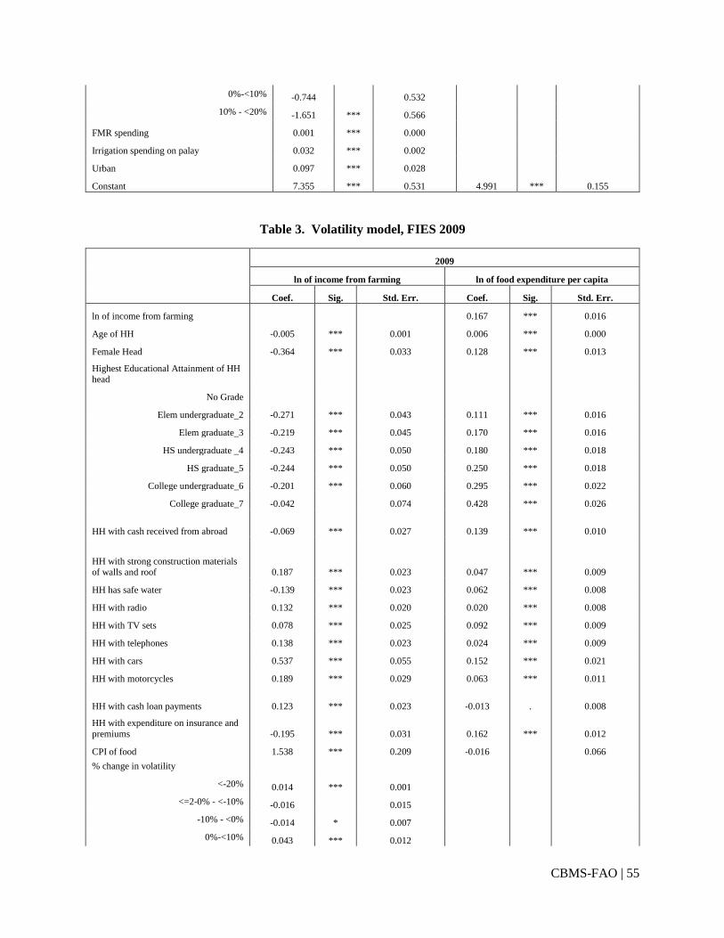
CBMS-FAO | 55

0%-<10% -0.744 0.532

10% - <20% -1.651 *** 0.566

FMR spending 0.001 *** 0.000

Irrigation spending on palay 0.032 *** 0.002

Urban 0.097 *** 0.028

Constant 7.355 *** 0.531 4.991 *** 0.155

Table 3. Volatility model, FIES 2009

2009

ln of income from farming ln of food expenditure per capita

Coef. Sig. Std. Err. Coef. Sig. Std. Err.

ln of income from farming 0.167 *** 0.016

Age of HH -0.005 *** 0.001 0.006 *** 0.000

Female Head -0.364 *** 0.033 0.128 *** 0.013

Highest Educational Attainment of HH head

No Grade

Elem undergraduate_2 -0.271 *** 0.043 0.111 *** 0.016

Elem graduate_3 -0.219 *** 0.045 0.170 *** 0.016

HS undergraduate _4 -0.243 *** 0.050 0.180 *** 0.018

HS graduate_5 -0.244 *** 0.050 0.250 *** 0.018

College undergraduate_6 -0.201 *** 0.060 0.295 *** 0.022

College graduate_7 -0.042 0.074 0.428 *** 0.026

HH with cash received from abroad -0.069 *** 0.027 0.139 *** 0.010

HH with strong construction materials of walls and roof 0.187 *** 0.023 0.047 *** 0.009

HH has safe water -0.139 *** 0.023 0.062 *** 0.008

HH with radio 0.132 *** 0.020 0.020 *** 0.008

HH with TV sets 0.078 *** 0.025 0.092 *** 0.009

HH with telephones 0.138 *** 0.023 0.024 *** 0.009

HH with cars 0.537 *** 0.055 0.152 *** 0.021

HH with motorcycles 0.189 *** 0.029 0.063 *** 0.011

HH with cash loan payments 0.123 *** 0.023 -0.013 . 0.008

HH with expenditure on insurance and

premiums -0.195 *** 0.031 0.162 *** 0.012

CPI of food 1.538 *** 0.209 -0.016 0.066

% change in volatility

<-20% 0.014 *** 0.001

<=2-0% - <-10% -0.016 0.015

-10% - <0% -0.014 * 0.007

0%-<10% 0.043 *** 0.012

CBMS-FAO | 56

10% - <20% -0.209 ** 0.098

>=20% 0.007 0.007

dummy % change in volatility

<-20% 0.932 *** 0.262

<=2-0% - <-10% -0.215 0.330

-10% - <0% 0.304 0.262

0%-<10% -0.038 0.266

10% - <20% 3.328 ** 1.536

FMR spending 0.001 *** 0.000

Irrigation spending on palay 0.022 *** 0.002

Urban 0.115 *** 0.028

Constant 6.969 *** 0.376 4.654 *** 0.167

Table 4. Temperature model, FIES 2009

2009.000

ln of income from farming ln of food expenditure per capita

Coef. Sig. Std. Err. Coef. Sig. Std. Err.

ln of income from farming 0.169 *** 0.016

Age of HH -0.005 *** 0.001 0.006 *** 0.000

Female Head -0.360 *** 0.033 0.129 *** 0.013

Highest Educational Attainment of HH head

No Grade

Elem undergraduate_2 -0.308 *** 0.043 0.112 *** 0.016

Elem graduate_3 -0.264 *** 0.045 0.171 *** 0.016

HS undergraduate _4 -0.280 *** 0.050 0.180 *** 0.018

HS graduate_5 -0.293 *** 0.050 0.251 *** 0.018

College undergraduate_6 -0.257 *** 0.060 0.295 *** 0.022

College graduate_7 -0.082 0.074 0.429 *** 0.026

HH with cash received from abroad -0.088 *** 0.027 0.139 *** 0.010

HH with strong construction materials of walls and roof 0.193 *** 0.023 0.046 *** 0.009

HH has safe water -0.172 *** 0.022 0.063 *** 0.008

HH with radio 0.145 *** 0.020 0.020 *** 0.008

HH with TV sets 0.057 *** 0.025 0.092 *** 0.009

HH with telephones 0.149 *** 0.023 0.024 *** 0.009

HH with cars 0.537 *** 0.054 0.152 *** 0.021

HH with motorcycles 0.186 *** 0.029 0.062 *** 0.011

HH with cash loan payments 0.121 *** 0.023 -0.013 . 0.008

HH with expenditure on insurance and

premiums -0.175 *** 0.031 0.162 *** 0.012

CBMS-FAO | 57

CPI of food 0.018 *** 0.002 0.000 0.001

Temperature

Decrease in min temp 0.990 *** 0.338

Increase in max temp -0.249 *** 0.064

Dummy Temperature

Decrease in min temp 0.728 *** 0.078

Increase in max temp 0.028 0.029

FMR spending 0.001 *** 0.000

Irrigation spending on palay 0.021 *** 0.002

Urban 0.108 *** 0.028

Constant 7.156 *** 0.271 4.638 *** 0.169

Table 5. IV validation tests, FIES 2009

Adjus

ted

model Rainfall Seasonality Volatility Temperature

Normality

Swilk

z

Prob>

z z

Prob>

z z

Prob>

z z

Prob>

z

9.046 0 8.734 0 9.223 0 9.341 0

Sktest

chi2(2)

Prob>

chi2 chi2(2)

Prob>

chi2 chi2(2)

Prob>

chi2 chi2(2)

Prob>

chi2

203.8 0 179.9 0 218.7 0 229.2 0

Sfranc

ia

z

Prob>

z z

Prob>

z z

Prob>

z z

Prob>

z

0.658 0.255 0.635 0.263 0.67 0.251 0.677 0.249

Test

Statistic

p-

value

Test

Statistic

p-

value

Test

Statistic

p-

value

Test

Statistic

p-

value

Underidentification

Ander

son

Chi-

sq(10)=550.

33 0

Chi-

sq(14)=551.

94 0

Chi-

sq(14)=500.

78 0

Chi-

sq(7)=475.

42 0

Cragg

-

Donal

d

Chi-

sq(10)=575.

34 0

Chi-

sq(14)=577.

10 0

Chi-

sq(14)=521.

40 0

Chi-

sq(7)=493.

97 0

Weak Instrument

Cragg

-

Donal

d

Wald 57.4 41.11 37.14 70.42

Ander

son-

Rubin

Wald

F(10,12631)

=33.33 0

F(14,12627)

=27.39 0

F(14,12627)

=26.50 0

F(7,12634)

=44.31 0

CBMS-FAO | 58

Ander

son-

Rubin

Wald

Chi-

sq(10)=334.

09 0

Chi-

sq(14)=384.

46 0

Chi-

sq(14)=372.

06 0

Chi-

sq(7)=310.

81 0

Overidentification

Sarga

n

Chi-

sq(9)=191.7 0

Chi-

sq(13)=259.

1 0

Chi-

sq(13)=222.

4 0

Chi-

sq(6)=166.

6 0

Ivendog

Wu-

Haus

man

F(1,12639)

=62.12 0

F(1,12639)

=44.8 0

F(1,12639)

=60.14 0

F(1,12639)

=62.12 0

Durbi

n-Wu-

Haus

man

Chi-

sq(1)=61.92 0

Chi-

sq(1)=44.4 0

Chi-

sq(1)=59.96 0

Chi-

sq(1)=61.9

2 0

Table 6. Rainfall model, CBMS 2007-2010

Variable Income from crop farming (log) With malnourished

Coe

f.

Std.

Err.

Sig

code

Robu

st SE

Robus

t Sig

Co

ef.

Std.

Err.

Sig

code

Robu

st SE

Robus

t Sig

Income from crop

farming (log)

-

0.2

48

0.01

1

*** 0.012 ***

Female head -

0.21

3

0.01

1

*** 0.012 *** -

0.0

57

0.02

2

*** 0.022 ***

Age of head 0.00

6

0.00

0

*** 0.000 *** -

0.0

07

0.00

0

*** 0.000 ***

Household size 0.02

6

0.00

1

*** 0.001 *** 0.0

54

0.00

2

*** 0.002 ***

IP indicator -

0.26

3

0.00

8

*** 0.008 *** 0.0

96

0.01

1

*** 0.011 ***

With OFW -

0.01

4

0.01

0

0.011

-

0.0

86

0.02

2

*** 0.022 ***

CBMS-FAO | 59

With safe water 0.05

6

0.00

6

*** 0.006 *** -

0.0

33

0.01

1

*** 0.011 ***

With radio 0.10

9

0.00

6

*** 0.006 *** -

0.0

48

0.01

0

*** 0.010 ***

With telephone 0.25

0

0.01

8

*** 0.021 *** -

0.1

72

0.04

5

*** 0.046 ***

With cellphone 0.18

2

0.00

6

*** 0.006 *** -

0.1

32

0.01

2

*** 0.013 ***

Availed govt prog -

0.04

9

0.00

6

*** 0.006 *** 0.1

41

0.01

0

*** 0.010 ***

Illness shock -

0.06

5

0.00

5

*** 0.005 *** 0.1

32

0.01

0

*** 0.010 ***

Urban 0.00

0

0.00

8

0.009

-

0.1

49

0.01

7

*** 0.017 ***

CPI - food 4.56

0

0.09

2

*** 0.095 *** 0.1

05

0.05

7

* 0.057 *

Education of head

Below elementary base

Elem level 0.14

2

0.01

2

*** 0.012 *** -

0.1

62

0.01

8

*** 0.018 ***

Elem grad 0.20

1

0.01

3

*** 0.013 *** -

0.2

06

0.02

1

*** 0.020 ***

HS level 0.17

3

0.01

4

*** 0.013 *** -

0.2

30

0.02

2

*** 0.021 ***

CBMS-FAO | 60

HS Grad 0.20

0

0.01

4

*** 0.013 *** -

0.2

93

0.02

2

*** 0.022 ***

Coll level 0.27

5

0.01

5

*** 0.015 *** -

0.2

88

0.02

7

*** 0.026 ***

Coll grad 0.37

1

0.01

9

*** 0.020 *** -

0.3

43

0.03

9

*** 0.039 ***

With agri org 0.13

6

0.01

6

*** 0.015 ***

With thresher 0.31

3

0.00

7

*** 0.007 ***

With dryer 0.21

2

0.01

1

*** 0.010 ***

With irrigation pump 0.27

8

0.01

0

*** 0.009 ***

Relative change in

rainfall

<-20% -

0.07

0

0.00

6

*** 0.006 ***

<=-20% - <-10% 0.02

7

0.00

4

*** 0.004 ***

-10% - <0% 0.03

1

0.00

4

*** 0.004 ***

0%-<10% 0.01

1

0.00

3

*** 0.004 ***

10% - <20% 0.02

5

0.00

3

*** 0.003 ***

>=20% 0.01

3

0.00

1

*** 0.001 ***

CBMS-FAO | 61

Relative change in rainfall

(dummies)

<-20% base

<=-20% - <-10% 1.69

7

0.15

5

*** 0.157 ***

-10% - <0% 1.52

0

0.14

6

*** 0.148 ***

0%-<10% 1.56

9

0.14

5

*** 0.146 ***

10% - <20% 1.31

5

0.14

8

*** 0.149 ***

>=20% 1.42

0

0.14

9

*** 0.151 ***

Cost of fertilizer -

1.41

8

0.03

6

*** 0.040 ***

Expenditure on farm

to market road

0.05

72

0.01

27

*** 0.013

8

***

Road density

category

4.25-6.31 base

6.31-6.37 -

0.65

50

0.01

82

*** 0.018

6

***

6.37-7.51 -

1.31

10

0.02

27

*** 0.023

0

***

7.51-7.62 -

0.79

20

0.01

88

*** 0.019

4

***

7.62-9.42 -

1.63

60

0.03

44

*** 0.038

0

***

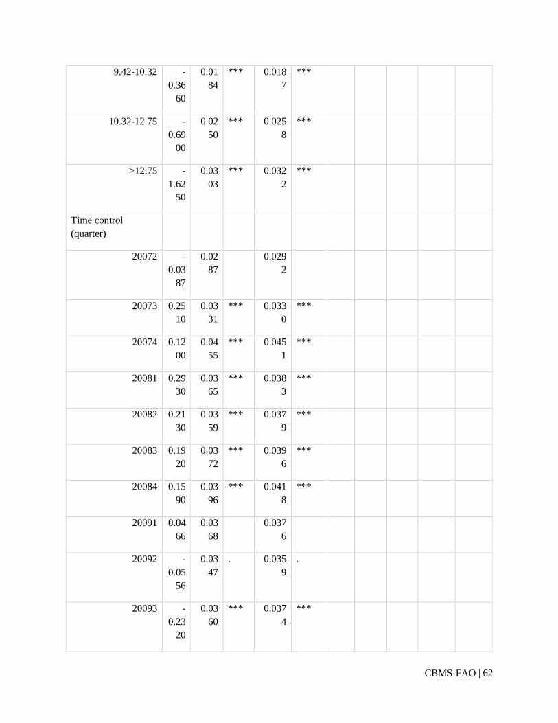
CBMS-FAO | 62

9.42-10.32 -

0.36

60

0.01

84

*** 0.018

7

***

10.32-12.75 -

0.69

00

0.02

50

*** 0.025

8

***

>12.75 -

1.62

50

0.03

03

*** 0.032

2

***

Time control

(quarter)

20072 -

0.03

87

0.02

87

0.029

2

20073 0.25

10

0.03

31

*** 0.033

0

***

20074 0.12

00

0.04

55

*** 0.045

1

***

20081 0.29

30

0.03

65

*** 0.038

3

***

20082 0.21

30

0.03

59

*** 0.037

9

***

20083 0.19

20

0.03

72

*** 0.039

6

***

20084 0.15

90

0.03

96

*** 0.041

8

***

20091 0.04

66

0.03

68

0.037

6

20092 -

0.05

56

0.03

47

. 0.035

9

.

20093 -

0.23

20

0.03

60

*** 0.037

4

***

CBMS-FAO | 63

20094 -

0.21

80

0.03

92

*** 0.040

8

***

20101 -

0.52

00

0.04

19

*** 0.043

6

***

20102 -

0.31

20

0.04

07

*** 0.042

1

***

20103 -

0.39

80

0.04

12

*** 0.043

1

***

20104 -

0.19

80

0.04

23

*** 0.044

7

***

adjustment -

0.03

16

0.01

63

* 0.017

3

*

Intercept 4.10

60

0.17

90

*** 0.181

0

*** 0.7

05

0.10

3

*** 0.114 ***

Wald's Chi-test for

exogeneity

315.

9

*** 249.1 ***

Sig. codes *** 2.5% ** 5% * 10% . 15%

Table 7. Rainfall seasonality model, CBMS 2007-2010

Variable Income from crop farming (log) With malnourished

Coe

f.

Std.

Err.

Sig

code

Robus

t SE

Robus

t Sig

Co

ef.

Std.

Err.

Sig

code

Robus

t SE

Robus

t Sig

Income from crop

farming (log)

-

0.2

58

0.011 *** 0.012 ***

CBMS-FAO | 64

Female head -

0.21

7

0.011 *** 0.012 *** -

0.0

60

0.022 *** 0.022 ***

Age of head 0.00

6

0.000 *** 0.000 *** -

0.0

07

0.000 *** 0.000 ***

Household size 0.02

5

0.001 *** 0.001 *** 0.0

54

0.002 *** 0.002 ***

IP indicator -

0.23

9

0.008 *** 0.008 *** 0.0

99

0.011 *** 0.011 ***

With OFW -

0.01

8

0.010 * 0.011 . -

0.0

87

0.022 *** 0.022 ***

With safe water 0.06

0

0.006 *** 0.006 *** -

0.0

32

0.011 *** 0.011 ***

With radio 0.11

8

0.006 *** 0.006 *** -

0.0

46

0.010 *** 0.010 ***

With telephone 0.24

6

0.018 *** 0.021 *** -

0.1

69

0.045 *** 0.045 ***

With cellphone 0.19

3

0.006 *** 0.006 *** -

0.1

29

0.012 *** 0.013 ***

Availed govt prog -

0.05

4

0.006 *** 0.006 *** 0.1

40

0.010 *** 0.010 ***

Illness shock -

0.06

4

0.005 *** 0.005 *** 0.1

31

0.010 *** 0.010 ***

Urban -

0.00

1

0.008

0.009

-

0.1

48

0.017 *** 0.017 ***

CBMS-FAO | 65

CPI - food 4.23

2

0.092 *** 0.095 *** 0.1

23

0.057 ** 0.057 **

Education of head

Below elementary base

Elem level 0.14

0

0.012 *** 0.012 *** -

0.1

59

0.018 *** 0.018 ***

Elem grad 0.20

0

0.013 *** 0.013 *** -

0.2

03

0.021 *** 0.020 ***

HS level 0.16

9

0.014 *** 0.013 *** -

0.2

27

0.022 *** 0.021 ***

HS Grad 0.19

4

0.014 *** 0.013 *** -

0.2

89

0.022 *** 0.022 ***

Coll level 0.26

5

0.015 *** 0.015 *** -

0.2

82

0.027 *** 0.026 ***

Coll grad 0.35

4

0.019 *** 0.020 *** -

0.3

36

0.039 *** 0.039 ***

With agri org 0.15

3

0.016 *** 0.016 ***

With thresher 0.32

5

0.007 *** 0.007 ***

With dryer 0.21

2

0.011 *** 0.010 ***

With irrigation

pump

0.28

1

0.010 *** 0.009 ***

Relative change in rainfall

seasonality

CBMS-FAO | 66

<-20% 0.00

3

0.001 *** 0.001 ***

<=-20% - <-10% 0.02

3

0.005 *** 0.005 ***

-10% - <0% -

0.00

3

0.003

0.003

0%-<10% 0.00

1

0.004

0.004

10% - <20% 0.00

3

0.004

0.004

>=20% 0.01

2

0.001 *** 0.001 ***

Relative change in rainfall

seasonality (dummies)

<-20% base

<=-20% - <-10% 0.22

8

0.069 *** 0.069 ***

-10% - <0% 0.02

0

0.034

0.035

0%-<10% 0.01

6

0.035

0.036

10% - <20% 0.05

5

0.064

0.067

>=20% -

0.07

8

0.044 * 0.045 *

Cost of fertilizer -

1.23

8

0.032 *** 0.035 ***

Road density

category

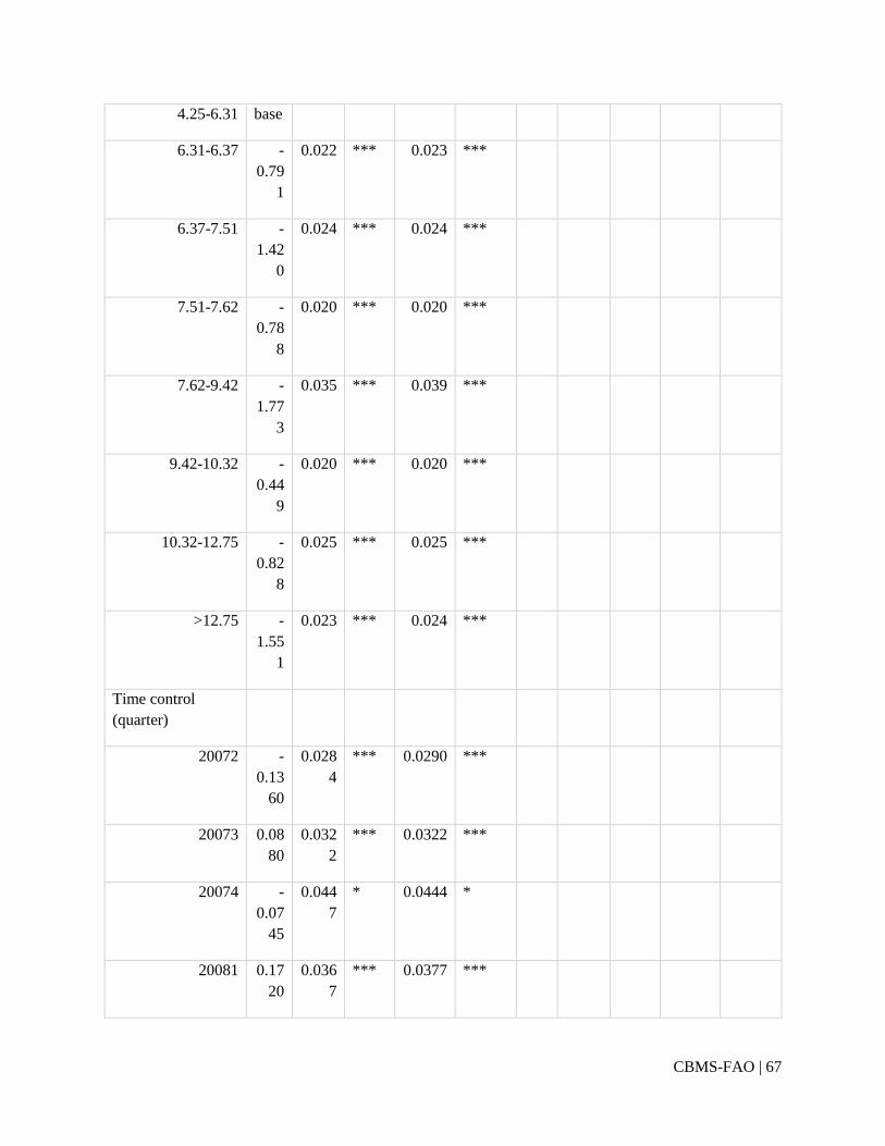
CBMS-FAO | 67

4.25-6.31 base

6.31-6.37 -

0.79

1

0.022 *** 0.023 ***

6.37-7.51 -

1.42

0

0.024 *** 0.024 ***

7.51-7.62 -

0.78

8

0.020 *** 0.020 ***

7.62-9.42 -

1.77

3

0.035 *** 0.039 ***

9.42-10.32 -

0.44

9

0.020 *** 0.020 ***

10.32-12.75 -

0.82

8

0.025 *** 0.025 ***

>12.75 -

1.55

1

0.023 *** 0.024 ***

Time control

(quarter)

20072 -

0.13

60

0.028

4

*** 0.0290 ***

20073 0.08

80

0.032

2

*** 0.0322 ***

20074 -

0.07

45

0.044

7

* 0.0444 *

20081 0.17

20

0.036

7

*** 0.0377 ***

CBMS-FAO | 68

20082 0.18

00

0.036

1

*** 0.0374 ***

20083 0.16

10

0.037

5

*** 0.0389 ***

20084 0.04

57

0.040

6

0.0419

20091 0.15

70

0.038

2

*** 0.0389 ***

20092 0.00

03

0.038

5

0.0395

20093 -

0.06

82

0.035

7

* 0.0366 *

20094 0.06

19

0.037

0

* 0.0380 .

20101 -

0.32

80

0.041

6

*** 0.0431 ***

20102 -

0.29

90

0.041

2

*** 0.0426 ***

20103 -

0.50

60

0.039

6

*** 0.0415 ***

20104 -

0.16

80

0.039

9

*** 0.0420 ***

adjustment -

0.00

79

0.016

7

0.0177

Intercept 5.93

10

0.102

0

*** 0.1050 *** 0.7

68

0.103 *** 0.115 ***

CBMS-FAO | 69

Wald's Chi-test for

exogeneity

336.7 *** 259.9 ***

Sig. codes *** 2.5% ** 5% * 10% . 15%

Table 8. Rainfall volatility model, CBMS 2007-2010

Variable Income from crop farming (log) With malnourished

Coe

f.

Std.

Err.

Sig

code

Robus

t SE

Robus

t Sig

Co

ef.

Std.

Err.

Sig

code

Robus

t SE

Robus

t Sig

Income from crop

farming (log)

-

0.2

56

0.011 *** 0.012 ***

Female head -

0.21

6

0.011 *** 0.012 *** -

0.0

60

0.022 *** 0.022 ***

Age of head 0.00

6

0.000 *** 0.000 *** -

0.0

07

0.000 *** 0.000 ***

Household size 0.02

4

0.001 *** 0.001 *** 0.0

54

0.002 *** 0.002 ***

IP indicator -

0.21

1

0.008 *** 0.008 *** 0.1

02

0.011 *** 0.011 ***

With OFW -

0.02

0

0.010 * 0.011 * -

0.0

87

0.022 *** 0.022 ***

With safe water 0.04

8

0.006 *** 0.006 *** -

0.0

33

0.011 *** 0.011 ***

With radio 0.12

5

0.006 *** 0.006 *** -

0.0

46

0.010 *** 0.010 ***

CBMS-FAO | 70

With telephone 0.24

0

0.018 *** 0.021 *** -

0.1

69

0.045 *** 0.046 ***

With cellphone 0.20

4

0.006 *** 0.006 *** -

0.1

29

0.012 *** 0.013 ***

Availed govt prog -

0.05

9

0.006 *** 0.006 *** 0.1

40

0.010 *** 0.010 ***

Illness shock -

0.06

7

0.005 *** 0.005 *** 0.1

31

0.010 *** 0.010 ***

Urban 0.01

1

0.008

0.009

-

0.1

48

0.017 *** 0.017 ***

CPI - food 3.98

2

0.095 *** 0.098 *** 0.1

27

0.058 ** 0.057 **

Education of head

Below elementary base

Elem level 0.15

3

0.012 *** 0.012 *** -

0.1

58

0.018 *** 0.018 ***

Elem grad 0.21

7

0.013 *** 0.013 *** -

0.2

01

0.021 *** 0.020 ***

HS level 0.18

4

0.014 *** 0.013 *** -

0.2

25

0.022 *** 0.021 ***

HS Grad 0.20

9

0.014 *** 0.013 *** -

0.2

88

0.022 *** 0.022 ***

Coll level 0.27

6

0.015 *** 0.015 *** -

0.2

82

0.027 *** 0.026 ***

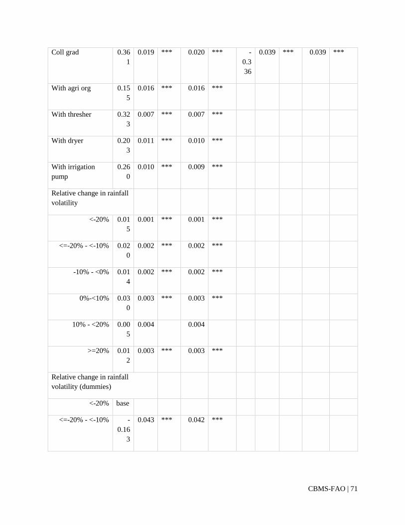
CBMS-FAO | 71

Coll grad 0.36

1

0.019 *** 0.020 *** -

0.3

36

0.039 *** 0.039 ***

With agri org 0.15

5

0.016 *** 0.016 ***

With thresher 0.32

3

0.007 *** 0.007 ***

With dryer 0.20

3

0.011 *** 0.010 ***

With irrigation

pump

0.26

0

0.010 *** 0.009 ***

Relative change in rainfall

volatility

<-20% 0.01

5

0.001 *** 0.001 ***

<=-20% - <-10% 0.02

0

0.002 *** 0.002 ***

-10% - <0% 0.01

4

0.002 *** 0.002 ***

0%-<10% 0.03

0

0.003 *** 0.003 ***

10% - <20% 0.00

5

0.004

0.004

>=20% 0.01

2

0.003 *** 0.003 ***

Relative change in rainfall

volatility (dummies)

<-20% base

<=-20% - <-10% -

0.16

3

0.043 *** 0.042 ***

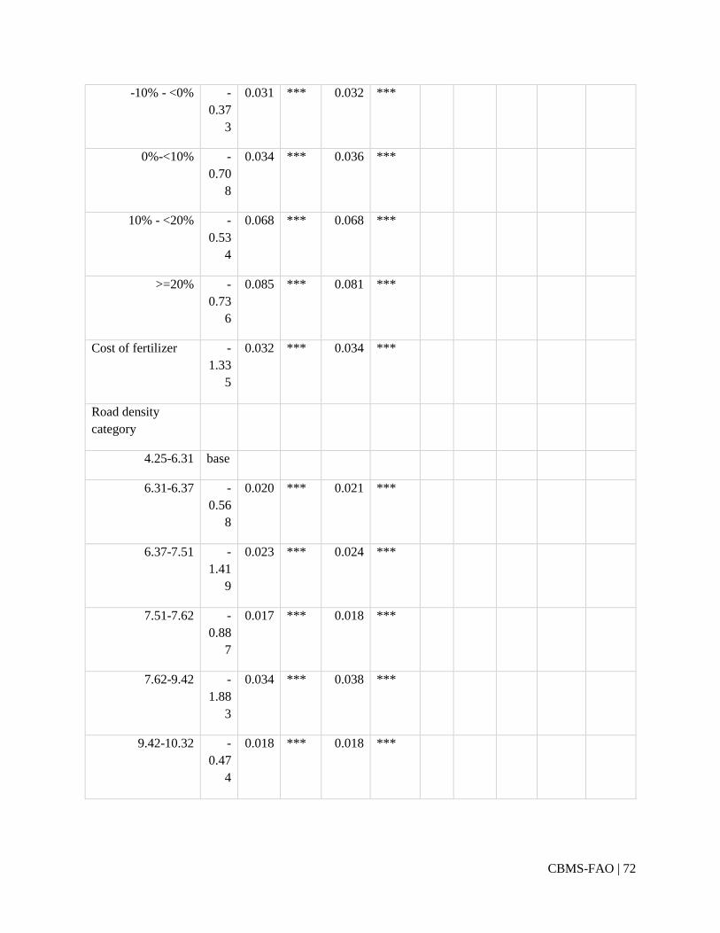
CBMS-FAO | 72

-10% - <0% -

0.37

3

0.031 *** 0.032 ***

0%-<10% -

0.70

8

0.034 *** 0.036 ***

10% - <20% -

0.53

4

0.068 *** 0.068 ***

>=20% -

0.73

6

0.085 *** 0.081 ***

Cost of fertilizer -

1.33

5

0.032 *** 0.034 ***

Road density

category

4.25-6.31 base

6.31-6.37 -

0.56

8

0.020 *** 0.021 ***

6.37-7.51 -

1.41

9

0.023 *** 0.024 ***

7.51-7.62 -

0.88

7

0.017 *** 0.018 ***

7.62-9.42 -

1.88

3

0.034 *** 0.038 ***

9.42-10.32 -

0.47

4

0.018 *** 0.018 ***

CBMS-FAO | 73

10.32-12.75 -

0.90

5

0.021 *** 0.021 ***

>12.75 -

1.71

5

0.022 *** 0.022 ***

Time control

(quarter)

20072 -

0.20

70

0.029

5

*** 0.0302 ***

20073 0.13

30

0.035

2

*** 0.0358 ***

20074 -

0.05

90

0.046

1

0.0458

20081 0.36

50

0.039

0

*** 0.0402 ***

20082 0.32

20

0.038

5

*** 0.0399 ***

20083 0.37

70

0.039

6

*** 0.0412 ***

20084 0.24

20

0.041

8

*** 0.0433 ***

20091 0.40

50

0.038

7

*** 0.0392 ***

20092 0.42

10

0.038

8

*** 0.0398 ***

20093 0.20

80

0.038

1

*** 0.0390 ***

20094 0.42

20

0.037

6

*** 0.0384 ***

CBMS-FAO | 74

20101 0.06

56

0.044

2

. 0.0455 .

20102 -

0.00

46

0.044

8

0.0461

20103 -

0.23

10

0.045

7

*** 0.0477 ***

20104 0.06

78

0.043

6

. 0.0454 .

adjustment -

0.08

27

0.016

1

*** 0.0171 ***

Intercept 6.67

40

0.107

0

*** 0.1110 *** 0.7

45

0.102 *** 0.114 ***

Wald's Chi-test for

exogeneity

330.8 *** 255.9 ***

Sig. codes *** 2.5% ** 5% * 10% . 15%

Table 9. Temperature model, CBMS 2007-2010

Variable Income from crop farming (log) With malnourished

Co

ef.

Std.

Err.

Sig

code

Robus

t SE

Robus

t Sig

Co

ef.

Std.

Err.

Sig

code

Robus

t SE

Robus

t Sig

Income from crop

farming (log)

-

0.2

53

0.011 *** 0.012 ***

Female head -

0.2

16

0.011 *** 0.012 *** -

0.0

59

0.022 *** 0.022 ***

CBMS-FAO | 75

Age of head 0.0

06

0.000 *** 0.000 *** -

0.0

07

0.000 *** 0.000 ***

Household size 0.0

25

0.001 *** 0.001 *** 0.0

54

0.002 *** 0.002 ***

IP indicator -

0.2

75

0.008 *** 0.008 *** 0.0

99

0.011 *** 0.011 ***

With OFW -

0.0

15

0.010

0.011

-

0.0

86

0.022 *** 0.022 ***

With safe water 0.0

43

0.006 *** 0.006 *** -

0.0

34

0.011 *** 0.011 ***

With radio 0.1

14

0.006 *** 0.006 *** -

0.0

47

0.010 *** 0.010 ***

With telephone 0.2

48

0.018 *** 0.021 *** -

0.1

70

0.045 *** 0.046 ***

With cellphone 0.1

97

0.006 *** 0.006 *** -

0.1

30

0.012 *** 0.013 ***

Availed govt prog -

0.0

52

0.006 *** 0.006 *** 0.1

41

0.010 *** 0.010 ***

Illness shock -

0.0

76

0.005 *** 0.005 *** 0.1

31

0.010 *** 0.010 ***

Urban 0.0

03

0.008

0.009

-

0.1

49

0.017 *** 0.017 ***

CPI - food 4.1

86

0.093 *** 0.095 *** 0.1

17

0.058 ** 0.057 **

Education of head

CBMS-FAO | 76

Below elementary bas

e

Elem level 0.1

49

0.012 *** 0.012 *** -

0.1

60

0.018 *** 0.018 ***

Elem grad 0.2

08

0.013 *** 0.013 *** -

0.2

03

0.021 *** 0.020 ***

HS level 0.1

71

0.014 *** 0.013 *** -

0.2

27

0.022 *** 0.021 ***

HS Grad 0.2

00

0.014 *** 0.013 *** -

0.2

90

0.022 *** 0.022 ***

Coll level 0.2

64

0.015 *** 0.015 *** -

0.2

84

0.027 *** 0.026 ***

Coll grad 0.3

49

0.019 *** 0.020 *** -

0.3

38

0.039 *** 0.039 ***

With agri org 0.1

46

0.016 *** 0.016 ***

With thresher 0.3

02

0.007 *** 0.007 ***

With dryer 0.2

05

0.011 *** 0.010 ***

With irrigation pump 0.2

45

0.010 *** 0.009 ***

Change in

temperatures

Change in minimum

temperature

0.6

39

0.042 *** 0.044 ***

CBMS-FAO | 77

Increase in minimum

temperature

-

0.3

33

0.047 *** 0.049 ***

Change in maximum

temperature

-

0.0

93

0.022 *** 0.021 ***

Increase in maximum

temp

0.0

89

0.028 *** 0.027 ***

Cost of fertilizer -

1.2

22

0.033 *** 0.035 ***

Expenditure on farm

to market road

0.0

19

0.013

0.014

Road density

category

4.25-6.31 bas

e

6.31-6.37 -

0.5

38

0.018 *** 0.019 ***

6.37-7.51 -

1.1

67

0.021 *** 0.021 ***

7.51-7.62 -

0.8

83

0.018 *** 0.019 ***

7.62-9.42 -

1.6

58

0.035 *** 0.038 ***

9.42-10.32 -

0.5

55

0.019 *** 0.019 ***

10.32-12.75 -

0.6

73

0.024 *** 0.026 ***

CBMS-FAO | 78

>12.75 -

1.7

23

0.032 *** 0.034 ***

Time control

(quarter)

20072 0.0

60

0.028 ** 0.028 **

20073 0.3

39

0.031 *** 0.030 ***

20074 0.2

19

0.044 *** 0.042 ***

20081 0.5

50

0.035 *** 0.036 ***

20082 0.5

13

0.034 *** 0.036 ***

20083 0.4

41

0.036 *** 0.038 ***

20084 0.2

70

0.039 *** 0.040 ***

20091 0.3

61

0.035 *** 0.035 ***

20092 0.2

28

0.033 *** 0.034 ***

20093 0.2

02

0.033 *** 0.034 ***

20094 0.5

19

0.033 *** 0.034 ***

20101 0.2

48

0.038 *** 0.039 ***

20102 0.3

98

0.040 *** 0.041 ***

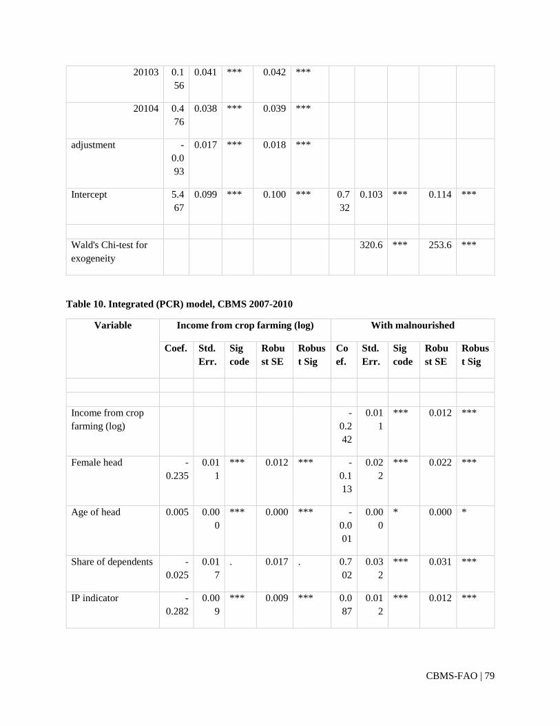
CBMS-FAO | 79

20103 0.1

56

0.041 *** 0.042 ***

20104 0.4

76

0.038 *** 0.039 ***

adjustment -

0.0

93

0.017 *** 0.018 ***

Intercept 5.4

67

0.099 *** 0.100 *** 0.7

32

0.103 *** 0.114 ***

Wald's Chi-test for

exogeneity

320.6 *** 253.6 ***

Table 10. Integrated (PCR) model, CBMS 2007-2010

Variable Income from crop farming (log) With malnourished

Coef. Std.

Err.

Sig

code

Robu

st SE

Robus

t Sig

Co

ef.

Std.

Err.

Sig

code

Robu

st SE

Robus

t Sig

Income from crop

farming (log)

-

0.2

42

0.01

1

*** 0.012 ***

Female head -

0.235

0.01

1

*** 0.012 *** -

0.1

13

0.02

2

*** 0.022 ***

Age of head 0.005 0.00

0

*** 0.000 *** -

0.0

01

0.00

0

* 0.000 *

Share of dependents -

0.025

0.01

7

. 0.017 . 0.7

02

0.03

2

*** 0.031 ***

IP indicator -

0.282

0.00

9

*** 0.009 *** 0.0

87

0.01

2

*** 0.012 ***

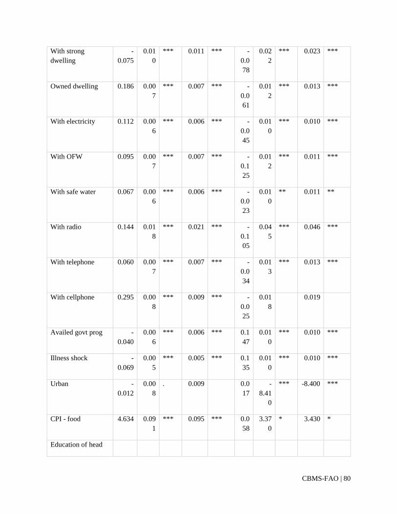
CBMS-FAO | 80

With strong

dwelling

-

0.075

0.01

0

*** 0.011 *** -

0.0

78

0.02

2

*** 0.023 ***

Owned dwelling 0.186 0.00

7

*** 0.007 *** -

0.0

61

0.01

2

*** 0.013 ***

With electricity 0.112 0.00

6

*** 0.006 *** -

0.0

45

0.01

0

*** 0.010 ***

With OFW 0.095 0.00

7

*** 0.007 *** -

0.1

25

0.01

2

*** 0.011 ***

With safe water 0.067 0.00

6

*** 0.006 *** -

0.0

23

0.01

0

** 0.011 **

With radio 0.144 0.01

8

*** 0.021 *** -

0.1

05

0.04

5

*** 0.046 ***

With telephone 0.060 0.00

7

*** 0.007 *** -

0.0

34

0.01

3

*** 0.013 ***

With cellphone 0.295 0.00

8

*** 0.009 *** -

0.0

25

0.01

8

0.019

Availed govt prog -

0.040

0.00

6

*** 0.006 *** 0.1

47

0.01

0

*** 0.010 ***

Illness shock -

0.069

0.00

5

*** 0.005 *** 0.1

35

0.01

0

*** 0.010 ***

Urban -

0.012

0.00

8

. 0.009

0.0

17

-

8.41

0

*** -8.400 ***

CPI - food 4.634 0.09

1

*** 0.095 *** 0.0

58

3.37

0

* 3.430 *

Education of head

CBMS-FAO | 81

Below elementary base

Elem level 0.127 0.01

2

*** 0.012 *** -

0.1

41

0.01

8

*** 0.018 ***

Elem grad 0.160 0.01

3

*** 0.160

-

0.1

71

0.02

1

*** 0.020 ***

HS level 0.110 0.01

4

*** 0.110

-

0.1

96

0.02

2

*** 0.021 ***

HS Grad 0.109 0.01

4

*** 0.109

-

0.2

59

0.02

2

*** 0.022 ***

Coll level 0.129 0.01

5

*** 0.129

-

0.2

51

0.02

7

*** 0.026 ***

Coll grad 0.165 0.01

9

*** 0.165

-

0.3

03

0.03

9

*** 0.039 ***

With agri org 0.123 0.01

6

*** 0.015 ***

With thresher 0.296 0.00

7

*** 0.007 ***

With dryer 0.191 0.01

1

*** 0.010 ***

With irrigation

pump

0.235 0.01

0

*** 0.009 ***

Principal

Components

1 0.043 0.00

2

*** 0.002 ***

2 0.080 0.00

3

*** 0.003 ***

CBMS-FAO | 82

3 -

0.033

0.00

3

*** 0.003 ***

4 -

0.065

0.00

3

*** 0.003 ***

5 -

0.030

0.00

3

*** 0.003 ***

Cost of fertilizer -

1.271

0.03

4

*** 0.037 ***

Expenditure on farm

to market road

0.046 0.01

3

*** 0.014 ***

Irrigation

expenditure

0.004 0.00

1

*** 0.001 ***

Road density

category

4.25-6.31 base

6.31-6.37 -

0.762

0.02

1

*** 0.021 ***

6.37-7.51 -

1.377

0.02

3

*** 0.023 ***

7.51-7.62 -

0.791

0.01

8

*** 0.018 ***

7.62-9.42 -

1.666

0.03

3

*** 0.037 ***

9.42-10.32 -

0.542

0.02

3

*** 0.024 ***

10.32-12.75 -

0.685

0.02

4

*** 0.025 ***

>12.75 -

1.669

0.03

2

*** 0.034 ***

Time control

(quarter)

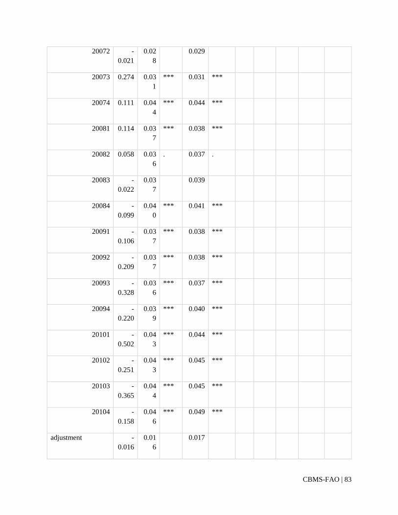
CBMS-FAO | 83

20072 -

0.021

0.02

8

0.029

20073 0.274 0.03

1

*** 0.031 ***

20074 0.111 0.04

4

*** 0.044 ***

20081 0.114 0.03

7

*** 0.038 ***

20082 0.058 0.03

6

. 0.037 .

20083 -

0.022

0.03

7

0.039

20084 -

0.099

0.04

0

*** 0.041 ***

20091 -

0.106

0.03

7

*** 0.038 ***

20092 -

0.209

0.03

7

*** 0.038 ***

20093 -

0.328

0.03

6

*** 0.037 ***

20094 -

0.220

0.03

9

*** 0.040 ***

20101 -

0.502

0.04

3

*** 0.044 ***

20102 -

0.251

0.04

3

*** 0.045 ***

20103 -

0.365

0.04

4

*** 0.045 ***

20104 -

0.158

0.04

6

*** 0.049 ***

adjustment -

0.016

0.01

6

0.017

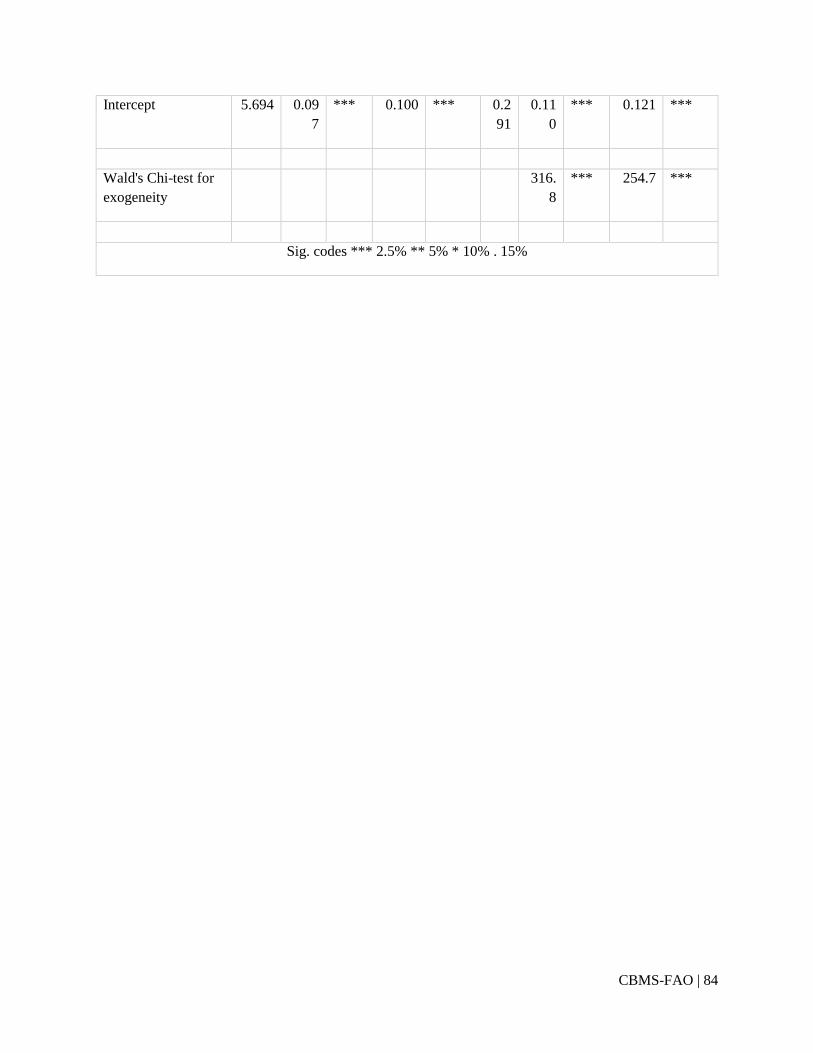
CBMS-FAO | 84

Intercept 5.694 0.09

7

*** 0.100 *** 0.2

91

0.11

0

*** 0.121 ***

Wald's Chi-test for

exogeneity

316.

8

*** 254.7 ***

Sig. codes *** 2.5% ** 5% * 10% . 15%

CBMS-FAO | 85

Table 11. Summary of diagnostics checking for FIES Data, 2009

Without

Outliers

Ori

gin

al

dat

a

Rainfall Seasonality Volatility Temperature

Number of Provinces

1st stage 80 72 66 60 74

2nd

stage 80 78 78 78 78

Number of Observations

1st

stage 12675 10768 10251 9448 10953

2nd

stage 12675 11690 11,043 11671 11011

Normality

Swilk z Prob>z z Prob>z z Prob>z z Prob>z

1st stage 14.62 0 14.66 0 14.63 0 14.55 0

2nd

stage 9.379 0 8.643 0 9.486 0 8.755 0

Sktest chi2(2)

Prob>c

hi2 chi2(2)

Prob>c

hi2 chi2(2)

Prob>c

hi2 chi2(2)

Prob>c

hi2

1st

stage 1593 0 1601 0 1571 0 1537 0

2nd stage 232.9 0 173.7 0 243 0 181.6 0

Sfranci

a z Prob>z z Prob>z z Prob>z z Prob>z

1st stage 0.824 0.205 0.824 0.205 0.824 0.205 0.823 0.205

2nd

stage 0.68 0.248 0.628 0.265 0.686 0.246 0.637 0.262

IVVIF

2nd stage

Variable VIF

IVHETTEST

Initial

Model

Pagan-Hall TS p-value

Pagan-Hall

TS p-value

Pagan-Hall

TS p-value

Pagan-Hall

TS p-value

Chi-

sq(30)=268.7 0

Chi-

sq(34)=244.1 0

Chi-

sq(34)=175.3 0

Chi-

sq(27)=159.6 0

NORMALITY

Test Statistic p-value Test Statistic p-value Test Statistic p-value Test Statistic p-value

Underidentification

Anders

on

Chi-

sq(10)=513.14 0

Chi-

sq(14)=502.48 0

Chi-

sq(14)=457.18 0

Chi-

sq(7)=437.37 0

Cragg-

Donald

Chi-

sq(10)=534.82 0

Chi-

sq(14)=523.25 0

Chi-

sq(14)=474.31 0

Chi-

sq(7)=453.02 0

Weak Instrument

Cragg-

Donald

Wald 53.36 37.27 33.79 64.58

Anderson-

Rubin

Wald

F(10,12631)=4

4.90 0

F(14,12627)=3

1.78 0

F(14,12627)=3

2.99 0

F(7,12634)=5

4.14 0

Anders

on-

Chi-

sq(10)=450.10 0

Chi-

sq(14)=446.18 0

Chi-

sq(14)=463.17 0

Chi-

sq(7)=379.77 0

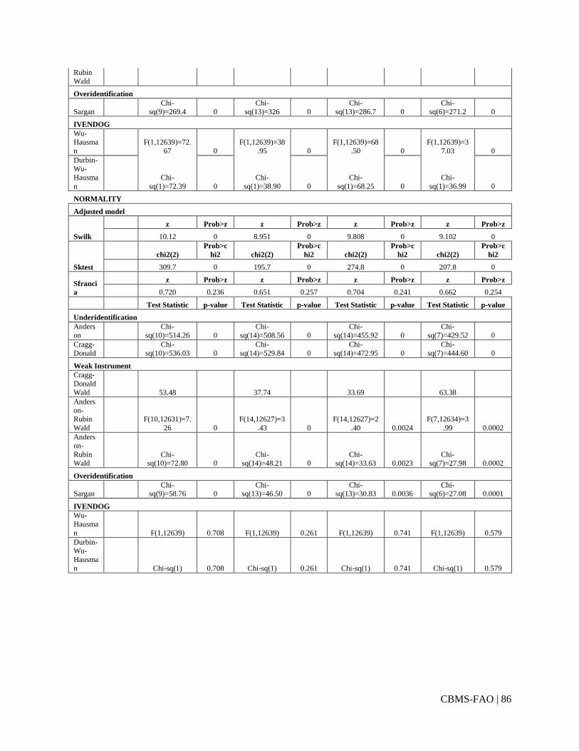
CBMS-FAO | 86

Rubin

Wald

Overidentification

Sargan

Chi-

sq(9)=269.4 0

Chi-

sq(13)=326 0

Chi-

sq(13)=286.7 0

Chi-

sq(6)=271.2 0

IVENDOG

Wu-Hausma

n

F(1,12639)=72.

67 0

F(1,12639)=38

.95 0

F(1,12639)=68

.50 0

F(1,12639)=3

7.03 0

Durbin-

Wu-Hausma

n

Chi-

sq(1)=72.39 0

Chi-

sq(1)=38.90 0

Chi-

sq(1)=68.25 0

Chi-

sq(1)=36.99 0

NORMALITY

Adjusted model

Swilk

z Prob>z z Prob>z z Prob>z z Prob>z

10.12 0 8.951 0 9.808 0 9.102 0

Sktest

chi2(2)

Prob>c

hi2 chi2(2)

Prob>c

hi2 chi2(2)

Prob>c

hi2 chi2(2)

Prob>c

hi2

309.7 0 195.7 0 274.8 0 207.8 0

Sfranci

a

z Prob>z z Prob>z z Prob>z z Prob>z

0.720 0.236 0.651 0.257 0.704 0.241 0.662 0.254

Test Statistic p-value Test Statistic p-value Test Statistic p-value Test Statistic p-value

Underidentification

Anders

on

Chi-

sq(10)=514.26 0

Chi-

sq(14)=508.56 0

Chi-

sq(14)=455.92 0

Chi-

sq(7)=429.52 0

Cragg-

Donald

Chi-

sq(10)=536.03 0

Chi-

sq(14)=529.84 0

Chi-

sq(14)=472.95 0

Chi-

sq(7)=444.60 0

Weak Instrument

Cragg-

Donald

Wald 53.48 37.74 33.69 63.38

Anders

on-

Rubin

Wald

F(10,12631)=7.

26 0

F(14,12627)=3

.43 0

F(14,12627)=2

.40 0.0024

F(7,12634)=3

.99 0.0002

Anders

on-

Rubin Wald

Chi-sq(10)=72.80 0

Chi-sq(14)=48.21 0

Chi-sq(14)=33.63 0.0023

Chi-sq(7)=27.98 0.0002

Overidentification

Sargan Chi-

sq(9)=58.76 0 Chi-

sq(13)=46.50 0 Chi-

sq(13)=30.83 0.0036 Chi-

sq(6)=27.08 0.0001

IVENDOG

Wu-

Hausma

n F(1,12639) 0.708 F(1,12639) 0.261 F(1,12639) 0.741 F(1,12639) 0.579

Durbin-Wu-

Hausma

n Chi-sq(1) 0.708 Chi-sq(1) 0.261 Chi-sq(1) 0.741 Chi-sq(1) 0.579

CBMS-FAO | 87

Table 12. Variance Inflation Factors, CBMS 2007-2010 model

Variable Rainfall Rainfall

seasonality

Rainfall

volatility

Temperatu

re

VIF 1/VI

F

VIF 1/VIF VIF 1/VIF VIF 1/VI

F

Female head 1.08 0.93 1.08 0.93 1.08 0.93 1.08 0.93

Age of head 1.44 0.70 1.43 0.70 1.43 0.70 1.43 0.70

Household size 1.23 0.81 1.23 0.82 1.23 0.81 1.23 0.82

IP indicator 1.62 0.62 1.50 0.67 1.47 0.68 1.70 0.59

With OFW 1.12 0.89 1.12 0.89 1.12 0.89 1.12 0.90

With safe water 1.15 0.87 1.14 0.87 1.14 0.87 1.14 0.88

With radio 1.11 0.90 1.11 0.90 1.10 0.91 1.11 0.90

With telephone 1.04 0.97 1.04 0.97 1.04 0.97 1.04 0.97

With cellphone 1.35 0.74 1.33 0.75 1.32 0.76 1.33 0.75

Availed govt prog 1.10 0.91 1.11 0.90 1.11 0.90 1.10 0.91

Illness shock 1.03 0.97 1.04 0.96 1.04 0.96 1.03 0.97

Urban 1.07 0.94 1.06 0.94 1.07 0.94 1.06 0.94

CPI - food 4.23 0.24 4.09 0.24 3.81 0.26 3.75 0.27

Education of head 1.09 0.91 1.10 0.91 1.10 0.91 1.09 0.92

Below elementary (base)

Elem level 4.83 0.21 4.77 0.21 4.75 0.21 4.80 0.21

Elem grad 4.10 0.24 4.04 0.25 4.02 0.25 4.08 0.25

HS level 3.46 0.29 3.41 0.29 3.39 0.30 3.43 0.29

HS Grad 3.92 0.25 3.86 0.26 3.84 0.26 3.89 0.26

Coll level 2.61 0.38 2.57 0.39 2.56 0.39 2.59 0.39

Coll grad 1.74 0.57 1.72 0.58 1.72 0.58 1.73 0.58

With agri org 1.02 0.98 1.02 0.98 1.02 0.98 1.02 0.98

With thresher 1.30 0.77 1.29 0.78 1.29 0.77 1.29 0.78

With dryer 1.32 0.76 1.32 0.76 1.32 0.76 1.32 0.76

With irrigation pump 1.44 0.69 1.45 0.69 1.44 0.69 1.44 0.69

<-20% 1.48 0.68 5.44 0.18 3.55 0.28

<=-20% - <-10% 1.65 0.61 1.56 0.64 1.71 0.58

-10% - <0% 2.72 0.37 4.15 0.24 2.04 0.49

0%-<10% 3.26 0.31 1.97 0.51 1.48 0.68

10% - <20% 3.52 0.28 2.69 0.37 1.33 0.75

>=20% 2.73 0.37 2.98 0.34 1.40 0.71

Decrease in TMIN

1.30 0.77

Increase in TMAX

1.46 0.68

Irrigation 3.58 0.28 1.76 0.57 2.28 0.44 1.80 0.55

Expenditure on farm to market

road

1.66 0.60 2.17 0.46 2.17 0.46 1.58 0.63

Mean VIF 2.15

2.19

1.99

1.90

CBMS-FAO | 88

Annex 2 – CBMS poverty maps based on predicted and projected malnutrition, rainfall and

temperature models

Map 7. Predicted and projected malnutrition using the rainfall model, Agusan del Norte

Map 8. Predicted and projected malnutrition using the temperature model, Agusan del Norte

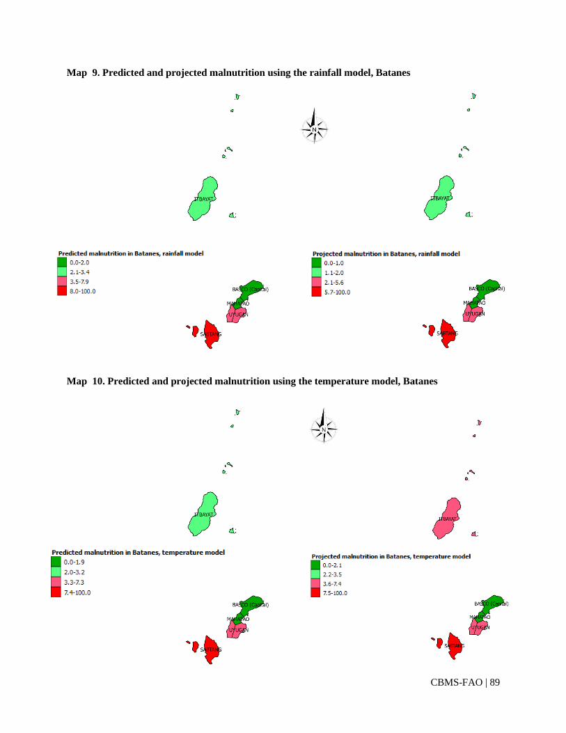
CBMS-FAO | 89

Map 9. Predicted and projected malnutrition using the rainfall model, Batanes

Map 10. Predicted and projected malnutrition using the temperature model, Batanes

CBMS-FAO | 90

Map 11. Predicted and projected malnutrition using the rainfall model, Batangas

Map 12. Predicted and projected malnutrition using the temperature model, Batangas

Map 12. Predicted and projected malnutrition using the temperature model, Batangas

CBMS-FAO | 91

Map 13. Predicted and projected malnutrition using the rainfall model, Benguet

Map 14. Predicted and projected malnutrition using the temperature model, Benguet

CBMS-FAO | 92

Map 15. Predicted and projected malnutrition using the rainfall model, Camarines Sur

Map 16. Predicted and projected malnutrition using the rainfall model, Camarines Sur

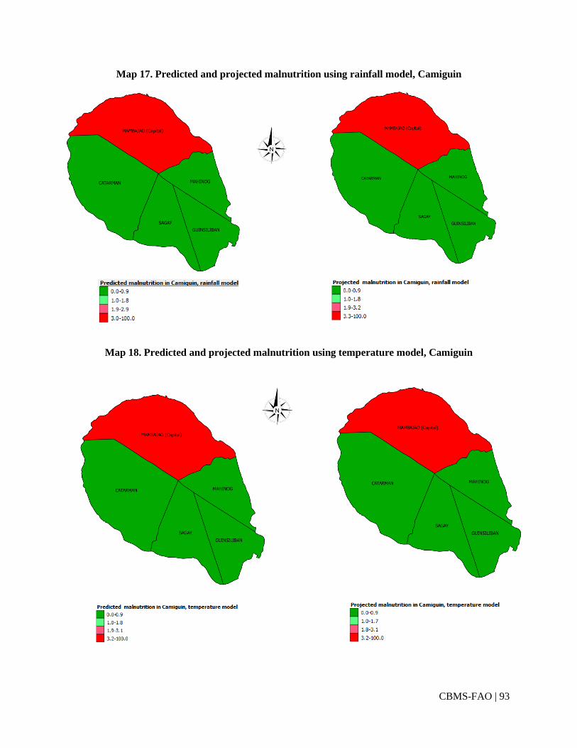
CBMS-FAO | 93

Map 17. Predicted and projected malnutrition using rainfall model, Camiguin

Map 18. Predicted and projected malnutrition using temperature model, Camiguin

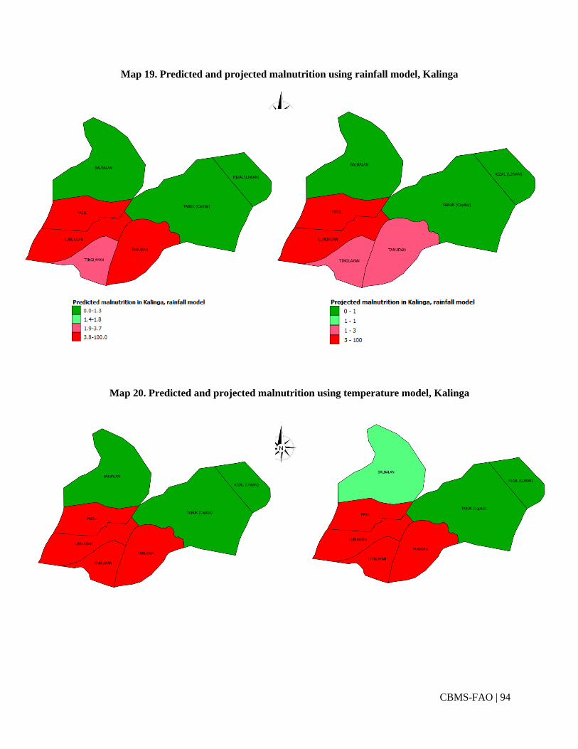
CBMS-FAO | 94

Map 19. Predicted and projected malnutrition using rainfall model, Kalinga

Map 20. Predicted and projected malnutrition using temperature model, Kalinga

CBMS-FAO | 95

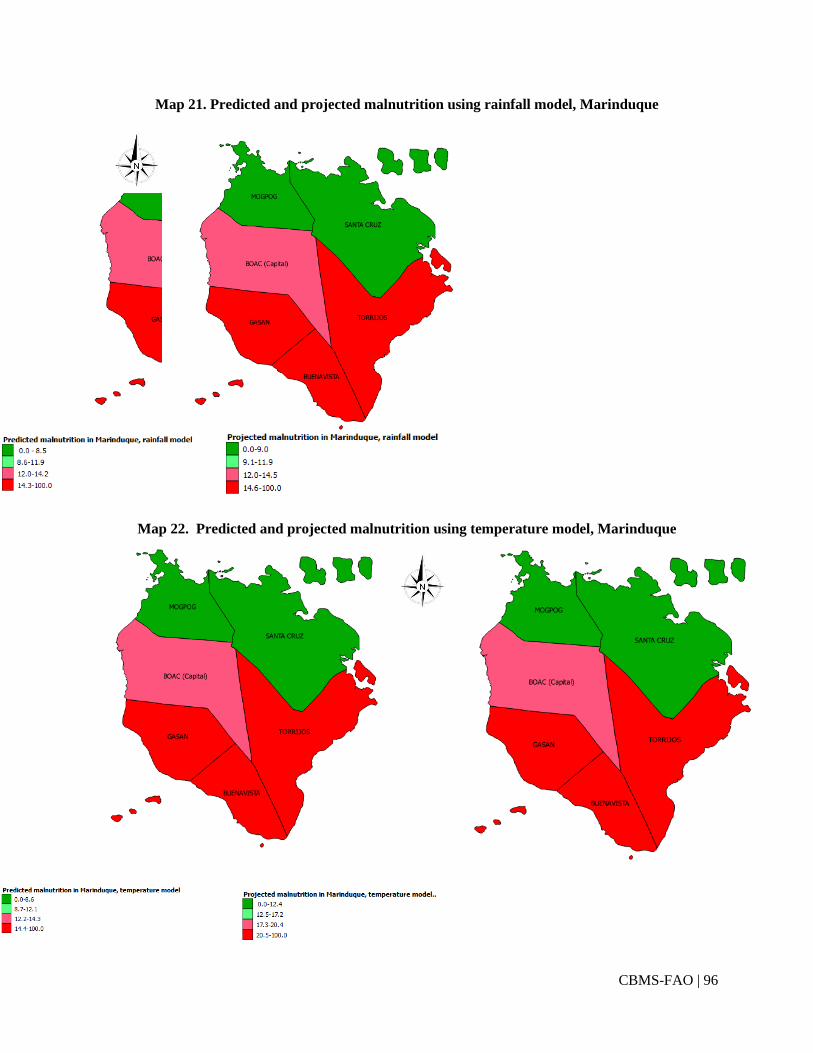
CBMS-FAO | 96

Map 21. Predicted and projected malnutrition using rainfall model, Marinduque

Map 22. Predicted and projected malnutrition using temperature model, Marinduque

CBMS-FAO | 97

Map 23. Predicted and projected malnutrition using rainfall model, Northern Samar

Map 24. Predicted and projected malnutrition using temperature model, Northern Samar

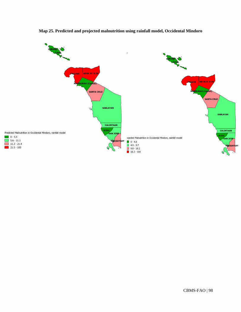
CBMS-FAO | 98

Map 25. Predicted and projected malnutrition using rainfall model, Occidental Mindoro

CBMS-FAO | 99

Map 26. Predicted and projected malnutrition using temperature model, Occidental Mindoro

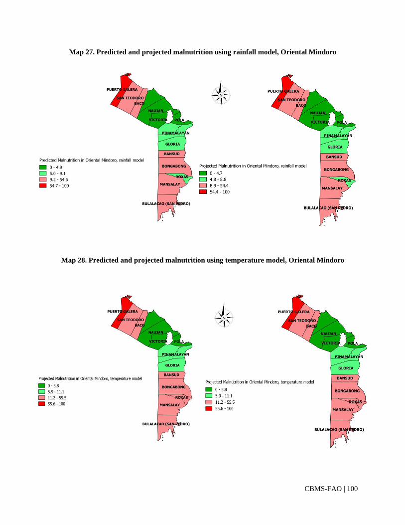
CBMS-FAO | 100

Map 27. Predicted and projected malnutrition using rainfall model, Oriental Mindoro

Map 28. Predicted and projected malnutrition using temperature model, Oriental Mindoro

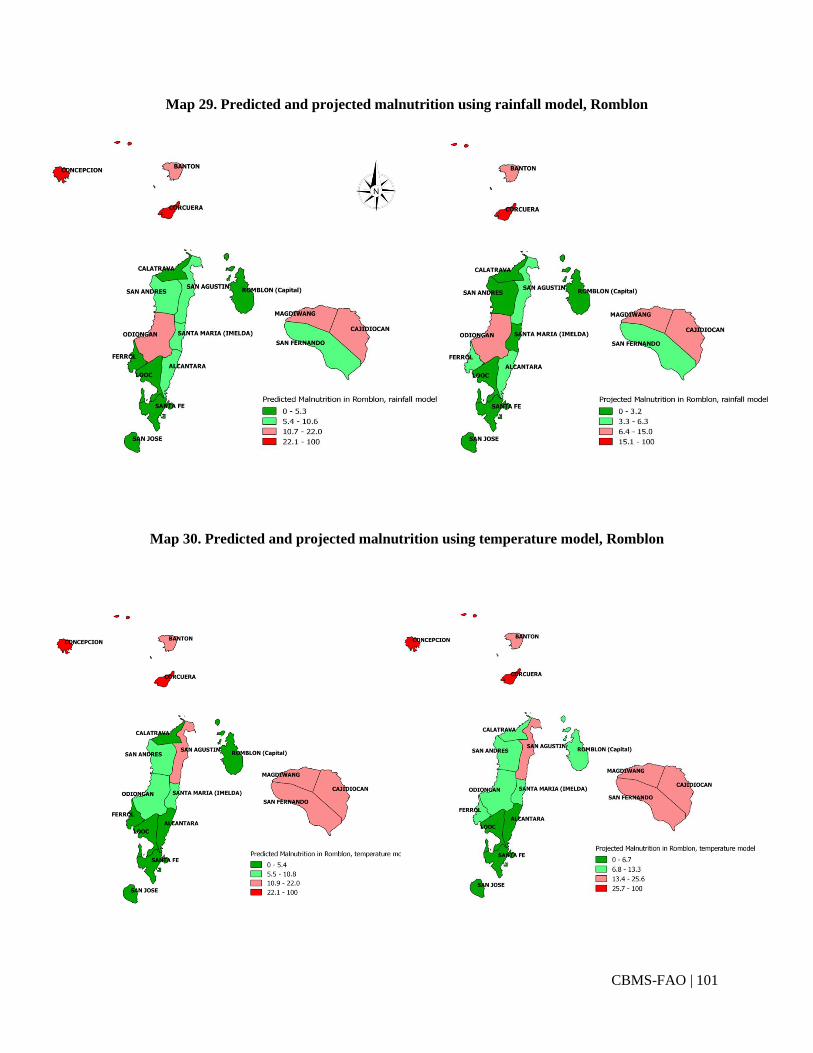
CBMS-FAO | 101

Map 29. Predicted and projected malnutrition using rainfall model, Romblon

Map 30. Predicted and projected malnutrition using temperature model, Romblon

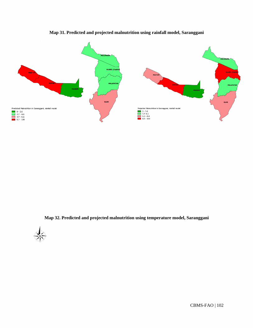
CBMS-FAO | 102

Map 31. Predicted and projected malnutrition using rainfall model, Saranggani

Map 32. Predicted and projected malnutrition using temperature model, Saranggani

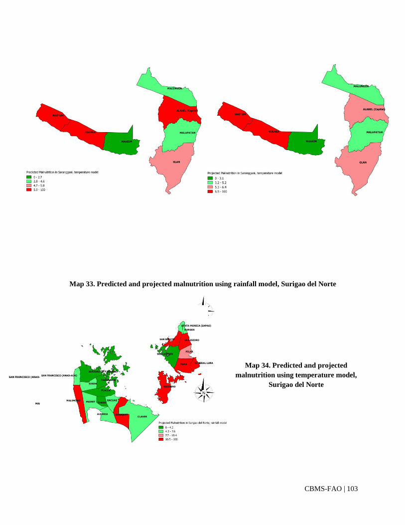
CBMS-FAO | 103

Map 33. Predicted and projected malnutrition using rainfall model, Surigao del Norte

Map 34. Predicted and projected

malnutrition using temperature model,

Surigao del Norte

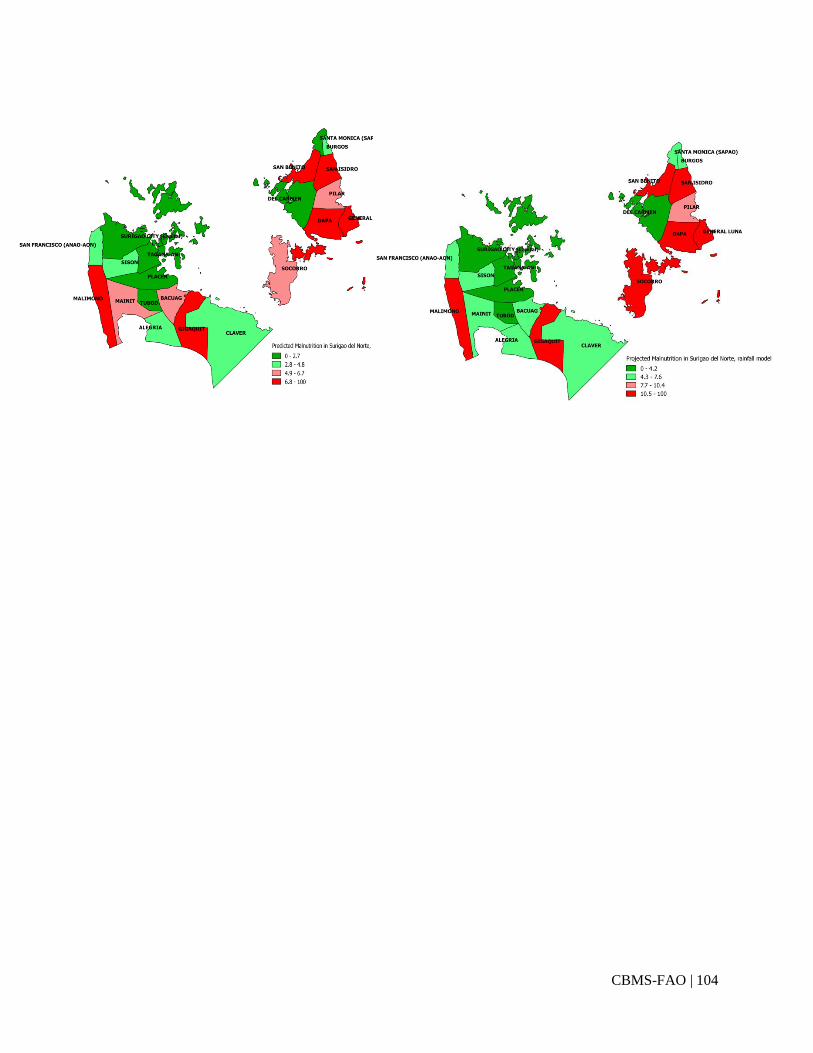
CBMS-FAO | 104

CBMS-FAO | 105

Map 35. Predicted and projected malnutrition using rainfall model, Surigao del Sur

Map 36. Predicted and projected malnutrition using temeprature model, Surigao del Sur

CBMS-FAO | 106

Map 37. Predicted and projected malnutrition using rainfall model, Tarlac

Map 38. Predicted and projected malnutrition using temperature model, Tarlac