Impacts of Climate Change on the Global Forest Sector

JOHN PEREZ-GARCIA1, LINDA A. JOYCE2, A.DAVID. MCGUIRE3 AND XIANGMING XIAO4

1Associate Professor, Center for International Trade in Forest Products, University of Washington, Seattle, WA 98195-2100, USA. 2Project Leader, Rocky Mountain Research Station, USDA Forest Service, Fort Collins, CO, 80526-2098, USA. 3Associate Professor, U. S. Geological Survey, Alaska Cooperative Fish and Wildlife Research Unit, University of Alaska, Fairbanks, AK 99775, USA. 4Research Assistant Professor Complex Systems Research Center, Institute for the Study of Earth, Oceans, and Space, University of New Hampshire, Durham, NH 03824, USA.

• George Perkins Marsh• Man and Nature Or, Physical Geography as

Modified by Human Action

• Originally published in 1864

Man’s Impact on Climate

Nordhaus: To Slow or Not To SlowGreenhouse Gas Emissions

What Has Been Done with Global Forest Sector

• Binkley et al. 1988

• Joyce et al. 1995

• Sohngen and Mendelsohn. 1998

Process Modeling Logic

CO2 Atmosphere Increase

Future climate regimes

Altered growth of forests

Impact on forest inventories

Changing economic timber supplies

Changes in production, consumption, prices and trade

Process Modeling Logic

CO2 Atmosphere Increase

Future climate regimes

Altered growth of forests

Impact on forest inventories

Changing economic timber supplies

Changes in production, consumption, prices and trade

EPPA/IGSM/GCMs

TEM

CGTM

Work with CGTM

• GCM and EPPA/IGSM

• TEM– NPP– Vegetative carbon

• Global in scope

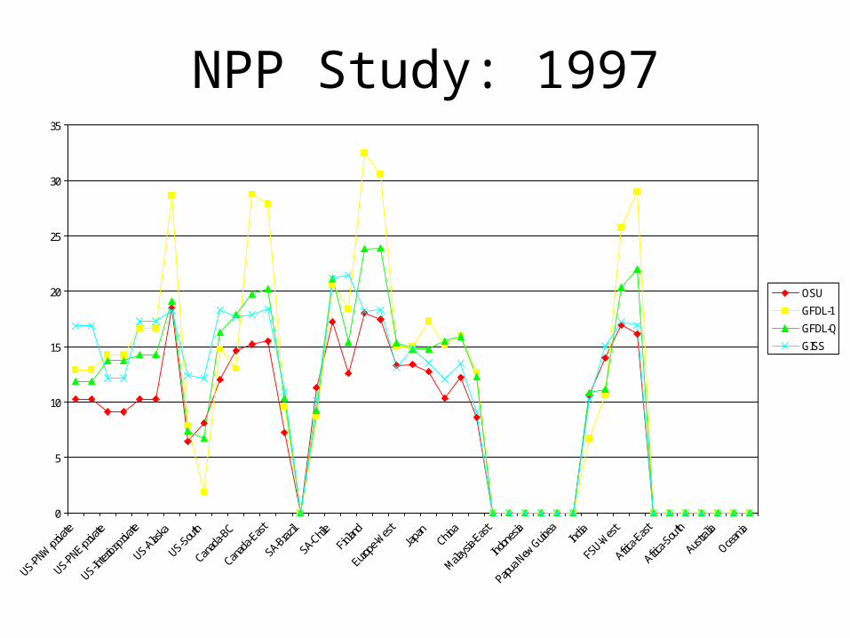
NPP Study: 1997

0

5

10

15

20

25

30

35

OSU

GFDL-1

GFDL-Q

GISS

Changes in Economic Surplus

-1.5

-1

-0.5

0

0.5

1

1.5

2

2.5

US Canada Chile Europe Japan NewZealand

Bil

lio

n U

S $

Timber Owners Mill Processors Consumers

Alternative Perspective: Annual Change versus Change from One Steady State to Another

0.00000.00020.00040.00060.00080.00100.00120.00140.00160.00180.0020

RRR 1

RRR 5

RRR 10

RRR 50

Global Economic Welfare Changes

0

2

4

6

8

10

12

14

16

18

20

LLHIntensive

LLHExtensive

RRRIntensive

RRRExtensive

HHLIntensive

HHLExtensive

Bil

lio

n $

"True" Transient Psuedo-Transient

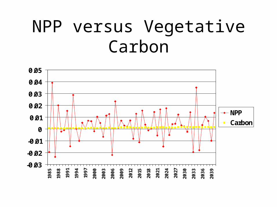
NPP versus Vegetative Carbon

-0.03

-0.02

-0.01

0

0.01

0.02

0.03

0.04

0.05

1985

1988

1991

1994

1997

2000

2003

2006

2009

2012

2015

2018

2021

2024

2027

2030

2033

2036

2039

NPPCarbon

Global Average NPP vs. Vegetative Carbon Over Time

0.00

0.05

0.10

0.15

0.20

0.25

nppcarbon

Harvests under NPP and Vegetative Carbon

0.000

0.005

0.010

0.015

0.020

0.025

0.030

CarbonNPP

What Do We Do

• Evaluate potential economic responses of the global forest sector to different scenarios of climate change produced from alternative levels of greenhouse gas emissions

• Economic baseline includes recent collapse of Asian economy and fall in production and consumption of wood products in Russia

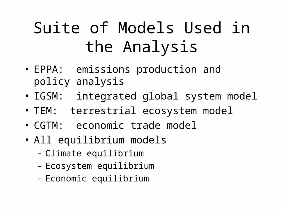
Suite of Models Used in the Analysis

• EPPA: emissions production and policy analysis• IGSM: integrated global system model• TEM: terrestrial ecosystem model• CGTM: economic trade model• All equilibrium models

– Climate equilibrium

– Ecosystem equilibrium

– Economic equilibrium

Climate Equilibrium

• Previously used 4 GCM’s– Did not consider atmospheric-ocean coupling– Did not consider atmospheric aerosols

• Doubling of CO2 climate

– Did not consider annual fluctuations

• Different treatment of radiative forcing associated with elevated CO2

Ecosystem Equilibrium

• Vegetation is in equilibrium– Responses are based on time-dependant

simulations of terrestrial biogeochemical models

• No successional dynamics

• No species migration dynamics

• No disturbance dynamics

Economic Equilibrium

• Partial equilibrium model

• Explicitly considers wood costs

• Explicitly considers trade in forest products

• Does not consider forest sector feedbacks to other economic sectors

• Does not consider carbon sequestration effects

IGSM

• Takes information from EPPA and creates transient climate change scenarios (Prinn et al., 1999).

• We use 3 of these scenarios RRR, HHL and LLH, where the reference set of parameters and assumptions generates the RRR scenario.

RRR

• Similar to the IS92a scenarios of IPPC

LLH

• Based on lower CO2 emissions from EPPA• Faster diffusion of heat into the ocean• Larger effects of cooling associated with

atmospheric aerosol• Largest heating effects associated with the

radiative forcing of increasing CO2• Leads to a smaller temperature change

relative to RRR

HHL

• Higher CO2 emissions from EPPA model• Slower diffusion of heat into the ocean• Smaller effects of cooling associated with

atmospheric aerosols• Smaller heating effects associated with

radiative forcing of doubling CO2• Leads to larger changes in temperature

relative to RRR

CGTM

• TEM-based changes in vegetative carbon are aggregated by timber types (softwood and hardwood).

• An index of proportional annual change in timber growing stock associated with changes in CO2 and climate for each grid cell in TEM is calculated.

CGTM Regions

United States (see Map 2)

Canada (see Map 3)

Central Americaand Mexico (CAM)

Northern South America (SAN)

Brazil (BRA)

Southern South America (SAS)

Chile (CHI)

Western Europe (EUW)

Sweden (SWE)

Finland (FIN)

Eastern Europe (EUE)

Japan (JPN)

Korea (KOR)China (CHN)Taiwan-Hong Kong (THK)

Former Soviet Union, West and East (SUW, SUE)

Middle East (MDE)

India (IND)Indochina (ICH)

Malaysia West (MAW) Malaysia East (MAE)Indonesia (IDN)

Papua New Guinea (PNG)

Australia (AUS)

Rest of Oceania (OCN)

New Zealand (NWZ)

East Africa (AFE)

Africa West (AFW)

Africa South (AFS)

Africa North (AFN)

Philippines (PHL)

Economic Variability

• Intensive economic margin or upward sloping supply curve– Constrain harvest to economic baseline for non-

responsive regions

• Extensive economic margin– Relaxes constrain on harvest for non-responsive

regions

General Results: More Production (More Growing Stock)

Prices

Quantity

General Results: Lower Prices (More Production)

Prices

Quantity

General Results: Greater Welfare

Prices

Quantity

HHL Climate Scenario

Intensive Margin Extensive Margin

Price Change -2.91% -3.09%

Harvest Change 2.73% 2.45%

Total Welfare Change 0.41% ($15.0 Billion) 0.44% ($15.8 Billion)

RRR Climate Scenario

Price Change -2.30% -2.44%

Harvest Change 2.36% 2.20%

Total Welfare Change 0.32% ($11.6 Billion) 0.32% ($11.6 Billion)

LLH Climate Scenario

Price Change -0.83% -0.86%

Harvest Change 1.49% 1.49%

Total Welfare Change 0.11%($3.9 Billion) 0.04%($1.8 Billion)

However

There is a lot of Regional Variability

Regional Variability

-0.05

0

0.05

0.1

0.15

0.2SWE

FIN

SAS

EUW

CHI

CBC

NWZ

CIN

CAM

INV

INB

ESB

WSV

WSB

ESV

AUS

CEA

JPN

EUE

CAL

USS

USN

IND

AFE

KOR

Which

Leads to Regional Price Changes

-8%

-7%

-6%

-5%

-4%

-3%

-2%

-1%

0%

US

Wes

t

US

So

uth

Can

ada

Ch

ile

Jap

an

Sca

nd

inav

ia

Wes

t E

uro

pe

Per

cen

t C

han

ge

ove

r B

asel

ine

HHL Extensive

HHL Intensive

RRR Extensive

RRR Intensive

LLH Extensive

LLH Intensive

From Left to Right

And

Regional Harvest Changes

-4%

-2%

0%

2%

4%

6%

8%

10%

12%

14%

US

Wes

t

US

So

uth

Can

ada

Ch

ile

Jap

an

Sca

nd

inav

ia

Wes

t E

uro

pe

Per

cen

t C

han

ge

ove

r B

asel

ine

HHL Extensive

HHL Intensive

RRR Extensive

RRR Intensive

LLH Extensive

LLH Intensive

From Left to Right

As A Result

Regional Welfare Changes

Climate and Economic Scenario LLH RRR HHL

Intensive Extensive Intensive Extensive Intensive Extensive Canada

PS Log (141.31) (150.05) (408.32) (403.20) (501.90) (469.64)

PS Product

(2,079.94) (1,826.15) (13,015.07) (12,153.60) (17,417.06) (15,905.72)

CS Product

420.71 472.49 2,674.10 3,064.06 3,607.84 4,079.74

Total (1,800.54) (1,503.71) (10,749.30) (9,492.74) (14,311.12) (12,295.61)

US South

PS Log (4,264.76) (4,204.01) (5,148.63) (4,744.64) (5,443.83) (4,681.10)

PS Product

(977.12) (1,593.15) (68.98) (953.29) 347.10 (620.82)

CS Product

929.18 1,546.86 6,937.38 7,500.80 9,449.16 9,762.38

Total (4,312.70) (4,250.30) 1,719.77 1,802.87 4,352.43 4,460.46

US West

PS Log (141.65) (392.31) (1,069.55) (990.57) (1,451.44) (1,597.59)

PS Product

902.79 756.45 6,354.85 5,927.72 8,623.98 7,898.11

CS Product

211.26 470.02 6.84 302.72 26.87 456.77

Total 972.41 834.16 5,292.14 5,239.87 7,199.41 6,757.29

Climate and Economic Scenario LLH RRR HHL

Intensive Extensive Intensive Extensive Intensive Extensive Chile

PS Log 4,651.67 2,607.28 3,878.78 1,704.07 3,461.73 1,310.97

PS Product

301.07 184.99 394.22 193.35 357.94 198.51

CS Product

52.48 285.68 350.86 633.65 473.40 740.39

Total 5,005.23 3,077.94 4,623.86 2,531.08 4,293.07 2,249.87

Japan

PS Log (267.87) (237.55) (1,426.67) (1,354.87) (2,004.41) (1,815.15)

PS Product

93.07 47.52 324.83 366.57 409.87 545.08

CS Product

415.24 188.76 2,524.34 2,303.96 3,591.51 3,102.81

Total 240.43 (1.26) 1,422.50 1,315.66 1,996.97 1,832.75

New Zealand

PS Log 2,334.25 1,197.51 1,850.93 724.93 1,511.43 419.14

PS Product

174.24 151.02 333.70 175.41 317.35 167.13

CS Product

30.96 6.05 293.56 251.97 394.18 334.01

Total 2,539.46 1,354.58 2,478.19 1,152.30 2,222.96 920.27

Climate and Economic Scenario LLH RRR HHL

Intensive Extensive Intensive Extensive Intensive Extensive West Europe

PS Log (514.66) (550.80) (643.81) (1,135.18) (713.30) (1,464.20)

PS Product

54.94 144.22 119.89 (308.87) 151.06 (526.80)

CS Product

1,097.11 1,927.21 1,701.45 5,141.96 1,996.60 6,796.51

Total 637.39 1,520.64 1,177.52 3,697.91 1,434.36 4,805.51

Finland

PS Log (244.59) (70.28) (353.33) (222.99) (407.77) (297.16)

PS Product

99.29 69.64 113.91 (14.37) 120.89 (78.05)

CS Product

52.97 163.92 75.76 289.36 87.21 358.37

Total (92.34) 163.28 (163.65) 52.00 (199.67) (16.84)

Sweden

PS Log (146.12) (186.46) (240.03) (488.95) (288.72) (654.34)

PS Product

201.79 264.58 294.23 247.63 342.08 224.43

CS Product

72.39 160.00 103.07 307.71 118.78 386.69

Total 128.06 238.11 157.27 66.39 172.14 (43.21)

Some Future Directions

soil Csoil N

Anthropogenic EmissionsPrediction and Policy

Analysis Model_________________

12 regions

agriculturalproduction

CO2, CH4, N2O, NOx,SOx, CO, CFCs

NaturalEmissions

Model______________

1deg x 1deg2.5 deg x 2.5 deg

Coupled

AtmosphericChemistry

and

Climate Model_________________

2D land-ocean(7.8 deg x 9 levels)

temperaturerainfall

oceanCO2

uptake

nutrients,pollutants

temperaturerainfall, clouds, CO2

TerrestrailEcosystem Model

___________________0.5 deg x 0.5 deg

landvegetation

change

landCO2

uptake

sealevel

CH4N2O

Forest ProductTrade Model

_______________

43 timber supply regions33 product demand regions

Perez-Garcia et al., submitted

ProposedResearchLinks

foresteconomics

changes ininventory

forestryland-uses