impacts of climate change scenarios on terrestrial...

I

Sara Filipa Marques Nunes Aparício

Licenciatura em Ciências de Engenharia do Ambiente

Impacts of Climate Change Scenarios on

Terrestrial Productivity and Biomass for

Energy in the Iberian Peninsula:

Assessment through the JSBACH model

Dissertação para obtenção do Grau de Mestre em Engenharia

do Ambiente, Perfil de Gestão e Sistemas Ambientais

Orientador: Maria Júlia Fonseca de Seixas, Ph.D, FCT-UNL

Coorientador: Nuno Miguel Matias Carvalhais, Ph.D., FCT-UNL

Júri:

Presidente: Prof. Doutora Maria Teresa Calvão Rodrigues

Arguente: Prof. Doutor João Manuel Dias dos Santos Pereira

Vogal: Prof. Doutora Maria Júlia Fonseca de Seixas

Vogal: Nuno Miguel Matias Carvalhais

Outubro, 2012

III

COPYRIGHT

The Faculty of Science and Technology and the New University of Lisbon entitled,

perpetual and without geographic boundaries, archive and publish this dissertation

through printed copies reproduced on paper or digital form, or by any other means

known or to be invented, and through the promotion scientific repositories and admit

your copying and distribution of educational objectives or research, not commercial, as

long as credit is given to the author and publisher.

V

Calvin : “You can't just turn on creativity like a

faucet. You have to be in the right mood”.

Hobbes : “What mood is that?”

Calvin : “Last-minute panic”.

In Calvin & Hobbes

VII

ACKNOWLEDGMENTS

I would like in first place to address my deep gratitude to my coordinator Júlia Seixas.

Thank you for guiding me throughout this thesis and for all your help in so many

fields, from recommending helpful literature review; to providing of a working space

and a computer (<with a blessing speed). Thank you as well for being so patient and

kind in the beginning, during my ramblings on the thesis project I would choose.

I would like as well to thank with equal gratitude to my sub-coordinator, Nuno

Carvalhais without whom this work wouldn’t be possible. Thank you for your

availability and for all the work that you have done in order to provide me the

JSBACH data. Thank you for sharing your knowledge in fruitful and enthusiastic

discussions.

My many thanks go to Christian Beer from the Max-Plank-Institut für Meteorologie,

who processed and share the JSBACH data upon which all my practical work was

based on.

I would like to express my gratitude to all my friends who supported me, and asked

me countless times about my thesis progress (well<grateful is not necessarily the word

for the last part), and I am sorry for not mention your names (this thesis is already big

enough, ok?). Nevertheless, I would like to address my special thanks to those who

had a particular and direct impact throughout the development of this thesis.

To Gonçalo and Favinha, for inviting me countless times to the catacombs of their

department, where day is night, creating the ideal atmosphere distractions-avoidant.

To Lina and Miguel – to the first, because part of this thesis was written inside Marineta

(beautiful specimen of camper) in Picos de Europa, and to the later because it had to be

recorded somewhere my blessing to your marriage (80 years from now). Please, choose

a shady place for the ceremony.

To Kathi, my sister-in-arms, despite the mere distance that separate us (2.750 km are

nothing), it was a pleasure to share small victories and huge sighs during our thesis

VIII

construction. Hopefully we will celebrate everything with Justin and Joela somewhere

in Europe?

To André, for being at this precise moment looking over my shoulder, helping me to

make sure (within last-minute pressure on writing the Acknowledgements) that, I will

not commit another horrible attack to English Grammar.

Thank you, my wonderful Grandparents and beautiful Mom (renewable and

inexhaustible sources of love and affection), and Sofia (my Sister since the Beginning of

Times). Thank you for supporting me with infinite patient.

I also want to thank my greatest life model< I have immense pride in being your

daughter.

IX

ABSTRACT Greenhouse gas abatement policies (as a measure of preventing further

contribution to global warming) are expected to increase the demand for renewable

sources of energy driving a growing attention on Biomass as a valuable option as a

renewable source of energy able to reduce CO2 emissions, by displacing fossil fuel use.

The vulnerability of the Iberian Peninsula (IP) to climate changes, along with the fact

that it is a water-limited region, drive a great concern and interest in understand the

potentials of biomass for energy production under projected climate changes, since

water shortage is a projected consequence of it.

Henceforth the goals stated for this work include the understanding of the impact

magnitude that climate changes and the solely effect of rising CO2 (in accordance to the

prescribed in A1B scenario from IPPC) have on biomass and productivity over the IP;

the modeling of the interannual variability in terrestrial productivity and biomass

across de region (having the period 1960-1990 as reference) and the energy potentials

derived by biomass in future scenarios (2060-2090 and 2070-2100 periods). The carbon

fluxes were modeled by JSBACH model and its results were handled using GIS and

statistical analysis. A better understanding of the applicability (and reliability) of this

model on achieving the latter stated goals was another goal purposed in this work.

IP has shown a broadly positive response to climate change, i.e. increased productivity

under scenarios admitting elevation of atmospheric CO2 concentration (increases in

GPP by ~41%; in forest NPP by ~54% and herbaceous NPP by ~36%, for 2060-2090

period), and smaller and negative response under scenarios disregarding rising CO2

levels (i.e. CO2 constant at 296ppm). The productivity and biomass correlation with

changing climate variables also differed between different CO2 scenarios. The increase

of water-use efficiency by 58% was as a result of CO2 fertilization effect, could explain

the increase of productivity, although many limitations of the model (such as disregard

of nitrogen cycle and land-use dynamics) poses many considerations to the

acceptability of results and the overestimating productivity comparatively to many

projections for the IP. Notwithstanding the comparison of changes in climate variables,

showed a great correlation of results with other authors.

A comprehensive analysis of biomass supply and its availability during scenarios with

elevated CO2, shown that by 2060-2090, residues from thinning and logging activities

over forest biomass have a potential of 0,165 and 0,495 EJ, and residues from

agricultural activities (herbaceous biomass) have a potential of 0,346 EJ under a HIGH-

YIELD scenario (assuming 40% of residues removal rate), corresponding to a share of

current energy consumption of 13, 42 and 30%, respectively. The reasonability of these

results was assessed by comparing with similar studies during the reference period.

Key Words: Biomass, Vulnerability, Climate Change, A1B IPCC Scenario,

Productivity, CO2 Fertilization & Water-use efficiency,

XI

RESUMO A Biomassa tem tido uma crescente atenção como opção relevante de fonte

energia renovável e emissor neutro de CO2 dadas as políticas de redução de gases de

efeito estufa (visando a prevenção do aquecimento global). A vulnerabilidade da

Península Ibérica (IP) face às mudanças climáticas, aliada ao facto de consistir numa

região onde a água é um factor limitante, levam a um grande interesse em

compreender as potencialidades da biomassa para produção energética em alterações

climáticas previstas, visto que a escassez de água é uma das consequências esperadas.

Os objectivos deste trabalho incluem assim a compreensão da magnitude dos impactos

que as mudanças climáticas e o efeito individual do aumento de CO2 (de acordo com o

prescrito no cenário A1B do IPPC) têm sobre a biomassa e produtividade sobre a IP; a

modelação da variabilidade interanual da produtividade terrestre e da biomassa

(tendo o período 1960-1990 como referência) e os potenciais energéticos de biomassa

em cenários futuros (períodos de 2060-2090 e 2070-2100). Os fluxos de carbono foram

modelados pelo modelo de JSBACH e os resultados foram tratados com SIG e análise

estatística. Uma melhor compreensão da aplicabilidade (e confiabilidade) deste modelo

na consecução das metas estabelecidas foi outro objectivo proposto neste trabalho.

A IP mostrou uma resposta amplamente positiva face a mudanças climáticas, ou seja,

aumento de GPP em ~ 41%; NPP florestal em ~ 54% e NPP de herbáceas em ~ 36%,

para período 2060-2090). Para cenários desconsiderando o aumento dos níveis de CO2

a resposta foi menor e negativa. A produtividade de biomassa e correlação com

variáveis climáticas mudança também diferiram entre os diferentes cenários de CO2. O

aumento da eficiência do uso da água em 58%, resultado de efeito de fertilização de

CO2, poderia explicar o aumento da produtividade, embora muitas limitações do

modelo (tais como a desconsideração do ciclo de nitrogénio e dinâmica do coberto

vegetal) coloca muitas considerações para quanto à aceitabilidade dos resultados,

dados os valores obtidos serem sobrestimados comparativamente a muitas projecções.

Não obstante a validação de mudanças em variáveis climáticas, mostrou uma grande

correlação de resultados com outros autores.

Uma análise detalhada disponibilidade de biomassa durante a cenários com CO2

elevado, mostraram, resíduos de desbaste e actividade madeireira (sobre biomassa

florestal) tem um potencial de 0.165 e 0.495 EJ, e resíduos de actividades agrícolas têm

um potencial de 0.346 EJ sob um cenário de alto rendimento (supondo uma taxa de

40% remoção de resíduos), correspondente a uma quota de consumo de energia actual,

de 13, 42 e 30%, respectivamente. A razoabilidade destes resultados foi validada

comparando com estudos semelhantes durante o período de referência.

Palavras-chave: Biomassa, Vulnerabilidade, Mudanças Climáticas, A1B Cenário

IPCC, Fertilização Produtividade, CO2 e do uso da água, eficiência

XIII

INDEX OF CONTENTS

Acknowledgments VII

Abstract XIX

Resumo XI

Index of Contents XIII

Index of Figures XV

Index of Tables XXI

tonnesAbbreviations XXV

1. Introduction

2. Climate change and Biomass for Energy

2.1. Climate Change Scenarios

2.2. Climate Change Impact on Energy Systems

2.3. Biomass as Energy Resources

2.3.1. Biomass definition and properties

2.3.2. Biomass resources for energy

2.3.3. Biomass contribution for mitigation of CO2 emission

2.3.4. Potential of Biomass for Energy

2.3.5. Biomass for Energy Competition Factors

2.4. Terrestrial Productivity and its relationship with Biomass

2.4.1. Absorbed photosynthetically active radiation (APAR)

2.4.2. Gross and Net Primary productivity

2.4.3. Carbon cycle

2.5. Impacts of Climate Change on Biomass potential

2.5.1. Temperature increase

2.5.2. Changes in precipitation patterns

2.5.3. Global NPP perspectives under water limitations

2.5.4. Elevated CO2 concentration

2.6. Assessing Terrestrial Productivity and Biomass

2.6.1. Dynamic Global Vegetation Models (DGVMs)

2.6.2. Main pitfalls and differences between DGVMs

3. Methodology to Estimate Productivity and Biomass Potential under

Climate Change

3.1. Study Area: the Iberian Peninsula

3.1.1. Bioclimatic patterns and zones

3.1.2. Climate Variability

3.1.3. Vegetation Cover

3.2. Modeling Tool: JSBACH

3.2.1. JSBACH overall description

3.2.2. BETHY module: Plant Functional Types (PFTs)

3.2.3. CBALANCE module

3.3. Model variables: inputs and outputs

3.4. Model datasets

3.4.1. WATCH data sets

1

7

7

11

13

14

18

24

27

36

42

43

47

49

51

53

54

56

59

59

63

64

68

71

71

73

76

79

79

82

90

90

92

92

XIV

3.4.2. ERA interim data sets

3.5. Simulation Condition and Scenarios

3.6. Data handling and treatment

3.6.1. Time aggregation

3.6.2. GIS Analysis

3.6.3. Statistical Analysis

3.7. Estimations of the potential of biomass for energy potentials

3.7.1. Biomass potentials

3.7.2. Biomass potential as resource

3.7.3. Biomass energy potential – Conversion into energy

4. Results and Discussion

4.1. Climate variables analysis – Reference Period

4.1.1. Land Surface Temperature (T)

4.1.2. Water Balance

4.1.3. Radiation Balance

4.1.4. Climate variables interaction

4.2. Carbon balance analysis – Reference Period

4.2.1. Gross Primary Production (GPP)

4.2.2. Net Primary Production (NPP)

4.2.3. Biomass

4.3. Climate changes analysis – Future Scenarios

4.3.1. Land Surface Temperature (T)

4.3.2. Water Balance

4.3.3. Radiation Balance

4.3.4. Climate variables interaction

4.4. Carbon balance analysis – Future Scenarios

4.4.1. Gross Primary Production (GPP)

4.4.2. Net Primary Production (NPP)

4.4.3. Biomass Potentials in Future Scenarios

4.5. Biomass Energy Potentials

5. Conclusions

5.1. Climate change and CO2 fertilization impact on productivity and

biomass

5.2. Biomass energy potentials

5.3. Considerations about the model and future research

6. References

7. Appendix

92

93

95

98

101

103

104

104

105

107

111

112

112

113

120

123

128

128

134

136

145

145

150

159

163

164

179

184

192

197

203

203

206

208

211

233

XV

INDEX OF FIGURES

Figure 1 - IPCCs' Representative concentrations pathways (RCPs) Source: adapted from Inman

(2011) ............................................................................................................................................ 8

Figure 2 - Schematic illustration of SRES scenarios. (Source: IPCC, 2000) .................................... 9

Figure 3 - CO2 emissions per year for the SRES scenarios (Source: IPCC, 2007) ........................ 10

Figure 4 - Atmospheric CO2 concentration projected under the 6 SRES marker and illustrative

scenarios assessed by to carbon cycle models: BERN (solid lines) and ISAM (dashed). (Source:

IPCC, 2001) .................................................................................................................................. 10

Figure 5 - Biomass model (Source: Gielen et al., 2001) .............................................................. 14

Figure 6 – The moisture percentage affects significantly the combustion quality and calorific

power of Forest Biomass (Source: Adapted from Brand, 2007) ................................................. 16

Figure 7 – The biomass components of a tree (Source: Redrawn from Juverics (2010)) ........... 20

Figure 8 - Dedicated cropping potential with perennials on released agricultural land in 2020

under reference and sustainability scenarios from Biomass Futures project (Source: Adapted

from Elbersen et al., 2012) .......................................................................................................... 35

Figure 9 - Relationship between above-ground net primary productivity (NPP) and above-

ground biomass (AGB) (Source: O’Neill & Angelis, 1981) ........................................................... 43

Figure 10 - Photosynthesis, respiration and Net Primary Productivity along temperature and

CO2 flux changes (Source: Whittaker & Likens, 1973) ................................................................ 45

Figure 11 – Relationships between NPP and temperature (a) and precipitation (b). (Source:

Whittaker & Likens, 1973) ........................................................................................................... 46

Figure 12- The changes of carbon balance and stocks from present o future –condition (Source:

Adapted from Ito & Oikawa, 2002) ............................................................................................. 51

Figure 13 - Stomata scheme (Source: Bonan, 2002) ................................................................... 55

Figure 15 – NPP under different scenarios: at the Present; assuming climate change; and

assuming climate and CO2 levels change (Source: Adapted from Rost et al., 2009). ................. 60

Figure 16 – DGMV scheme (Source: Cramer et al., 2001)........................................................... 66

Figure 17 – Map of the Iberian Peninsula – the darker brown is assigned to heights over

1000m; light brown is assigned to heights ranging between 500 and 1000m (i.e. high plateaus)

and the greenish color are assigned to heights lower than 500m (Source: Solarnavigator.net)

..................................................................................................................................................... 72

Figure 18- Köppen-Geiger Climate Classification for the Iberian Peninsula and the Balearic

Islands (Source: AEMET, 2000) .................................................................................................... 73

Figure 19 -Iberian Peninsula Bioclimatic zones - In accordance with Rivas-Martìnez et al. (2004)

..................................................................................................................................................... 75

Figure 20 - Monthly mean precipitation and temperature of temperate zone (left) and

Mediterranean zone (right) ......................................................................................................... 75

Figure 21 - Interactions between JSBACH and ECHAM5 ............................................................. 80

Figure 22 - JSBACH modules scheme .......................................................................................... 81

Figure 23 –BETHY scheme ........................................................................................................... 83

Figure 24 - Gridl cell example ...................................................................................................... 84

Figure 25 - Examples of soft traits and associated functions (Source: Canadell et al., 2007) .... 85

Figure 26 - The tilling approach (Source: Adapted from Brovnik et al., 2009) ........................... 86

Figure 27- Cover Type per tile ..................................................................................................... 89

XVI

Figure 28 - Scheme of different Carbon pools for different PFTs ............................................... 90

Figure 29 - CBALCANCE Carbon Pool model ............................................................................... 91

Figure 30 – Global carbon dioxide emissions (Gt(C)/year) for scenarios A1F1, A1R and A1B

(IPCC, 2000) ................................................................................................................................. 95

Figure 31 - Reference Period and Future Scenarios considered for the results ......................... 96

Figure 32 - Atmospheric CO2 concentrations during the Reference Period and the Future

Scenarios ..................................................................................................................................... 96

Figure 33 - Assessments from possible comparisons between Scenarios C1, C2, E1, E2 and the

Reference Period ......................................................................................................................... 97

Figure 34 - Overall Methodology Scheme ................................................................................. 100

Figure 35 - Flowchart: creating an image with different units - example for temperature

(degrees Kelvin to degrees Celsius conversion example) ......................................................... 101

Figure 36 – Procedure to evaluate percentage change of land surface temperature between

Temperature C1 (Scenario C1) and Temperature C2 (Scenario C2) .......................................... 102

Figure 37 - Procedure to evaluate ratios GPP between reference period and scenario C1 ..... 103

Figure 38 - Methodology applied to assessment of residue and energy potentials for forest

biomass sources (Tree) and Herbaceous biomass sources (Grasses) ....................................... 109

Figure 39 – Mean Annual Land Surface Temperature during the Reference Period [1060-1990]

................................................................................................................................................... 112

Figure 40 – Histogram and Statistical analysis of Mean Annual Land Surface Temperature over

the Iberian Peninsula during the Reference Period [1960-1990] ............................................. 113

Figure 41 – Mean Annual Precipitation during the Reference Period [1060-1990] ................. 113

Figure 42 - Histogram and Statistical analysis of Mean Annual Precipitation over the Iberian

Peninsula during the Reference Period [1960-1990] ................................................................ 115

Figure 43 – Histogram of soil moisture content of layer I [m] of layers 1,2,3,4 and 5 during

[1960-1990] ............................................................................................................................... 116

Figure 44-Mean Annual Soil Moisture Content during the Reference Period [1060-1990] and

comparison with the Iberian River Basins (Source: ) ................................................................ 117

Figure 45 - Histogram and Statistical analysis of Mean Annual Water Soil Content over the

Iberian Peninsula during the Reference Period [1960-1990].................................................... 118

Figure 46 – Mean Annual Evapotranspiration during the Reference Period [1060-1990] ....... 119

Figure 47 - Histogram and Statistical analysis of Mean Annual Evapotranspiration over the

Iberian Peninsula during the Reference Period [1960-1990].................................................... 120

Figure 48 - Mean Annual Photosynthetically Active Radiation map during the Reference

Scenario ..................................................................................................................................... 120

Figure 49 - - Mean Annual Absorbed Photosynthetically Active Radiation during the Reference

Period ........................................................................................................................................ 122

Figure 50 - Histogram and Statistical analysis of Mean Annual APAR over the Iberian Peninsula

during the Reference Period [1960-1990] ................................................................................ 122

Figure 51 - Ratio APAR/PAR during the Reference Period ........................................................ 123

Figure 52 - Correlation between climate variables during the Reference Period .................... 127

Figure 53 – Mean Annual Gross Primary Production (GPP) during the Reference Period [1960-

1990] ......................................................................................................................................... 128

Figure 54 - Relationship between GPP and Precipitation and GPP and Evapotranspiration


XVII

Figure 55 - Comparison of spatial distribution between GPP, P and ET during [1960-1990] ... 130

Figure 56 –The relationship between GPP and APAR at the IP during the 1960-1990 period. 131

Figure 57 - Mean Annual WUE during reference period........................................................... 132

Figure 58 - Mean Annual LUE during the Reference Period ..................................................... 133

Figure 59- Mean Annual Forest Net Primary Production (NPP) during the Reference Period

[1960-1990] ............................................................................................................................... 134

Figure 60 - Mean Annual Herbaceous Net Primary Production (NPP) during the Reference

Period [1960-1990] ................................................................................................................... 135

Figure 61 - Regression analysis between mean annual GPP and NPP (from all biomass) over the

Iberian Peninsula during the Reference Period ........................................................................ 136

Figure 62 - Mean Annual Forest Biomass Density during Reference Period [1960-1990] ........ 136

Figure 63 - Mean Annual Herbaceous Biomass Density during Reference Period [1960-1990]

................................................................................................................................................... 137

Figure 64 - Statistical analysis of Mean Annual Forest Biomass during [1960-1990] ............... 138

Figure 65 - Statistical analysis of Mean Annual Herbaceous Biomass during [1960-1990] ...... 138

Figure 66 - Percentage and absolute values of Forest and Herbaceous Biomass during the

Reference Period [1960-1990] .................................................................................................. 139

Figure 67 - Estimations of Biomass assigned to each PFT, during the Reference Period [1960-

1990] ......................................................................................................................................... 140

Figure 68 - Correlation between mean annual temperature and herbaceous/forest biomass


Figure 69 - Correlation between mean annual precipitation and herbaceous/forest biomass


Figure 70 - Correlation between mean annual ET and herbaceous/forest biomass during the


Figure 71 - Correlation between mean annual SWC and herbaceous/forest biomass during the


Figure 72 - Correlation between radiation variables and herbaceous/forest biomass during the


Figure 73 - Mean Annual Land Surface Temperature projected for scenario C1 [2060-2090] . 146

Figure 74 – Histograms and Statistical analysis of Land Surface Temperature for Scenarios C1

and C2 ........................................................................................................................................ 147

Figure 75 – Multi-Model Averages and Assessed Ranges for Surface Warming (Source: Adapted

from IPCC, 2007) ....................................................................................................................... 147

Figure 76 - Percentage Change of Mean Annual Land Surface Temperature between Reference

Period [1960-1990] and Scenario C1 [2060-2090] .................................................................... 148

Figure 77 - Percentage Change of Mean Annual Land Surface Temperature between Scenario

C1 [2060-2090] and Scenario C2 [2070-2100] .......................................................................... 149

Figure 78 - Annual Mean Precipitation during Scenario C1 [2060-2090] ................................. 150

Figure 79 - Histograms and Statistical analysis of Precipitation for Scenarios C1 and C2 ........ 150

Figure 80 - Percentage Change of Mean Annual Precipitation between Reference Period [1960-

1990] and Scenarios C1 (upper image) and Scenario C2 (bottom). In this case, positive change

refers to decrease in precipitation. Redish areas present higher decreases in precipitation and

greenish areas present lower decreases in precipitation. ........................................................ 151

Figure 81 - min c1~5,2 mm/m2/year min c24,8 ....................................................................... 152

XVIII

Figure 82 – Number of models which simulate a precipitation increase between the time

periods 2080-2099 and 1980-1999 for the scenario A1B (Source: Höschel et al., n.d.) ........... 153

Figure 83 - Time series of globally averaged precipitation change (%) from various coupled

models for Scenario A1B and E1, relative to the 1980-199 annual average (Source: Adapted

from Höschel et al., n.d.) ........................................................................................................... 153

Figure 84 - Mean Annual Soil Moisture Content during Scenario C1 [2060-2090] ................... 154

Figure 85 - Histograms and Statistical Analysis of Mean Annual SWC during Scenarios C1, C2, E1

and E2 ........................................................................................................................................ 155

Figure 86 - Multi-model (10 models) mean change in soil moisture content (%). Changes are

annual means for the SRES A1B scenario for the period 2080 to 2099 relative to 1980 to 1999.

The stippled marks the locations where at least 80% of models agree on the sign of the mean

change (Source: IPCC, 2007) ..................................................................................................... 156

Figure 87 - Mean Annual Evapotranspiration during Scenario C1 [2060-2090] ....................... 156

Figure 88 - Histograms and Statistical Analysis of Mean Annual Evapotranspiration during

Scenarios C1, C2, E1 and E2 ...................................................................................................... 157

Figure 89 - Differences between global mean ET during the period 1960-1990 and 2070-2100.

Simulation results from ECHAM5 with IPCC climate scenario A1B (Source: Kim et al., 2002) . 158

Figure 90 - Percentage Change of Mean Annual PAR between the Reference Period and

Scenario C1 [2060-2090] ........................................................................................................... 159

Figure 91 - Mean Annual APAR during Scenarios C1 and Scenario E1 [2060-2090] ................. 160

Figure 92 -Histograms and Statistical Analysis of Mean Annual APAR during Scenarios C1, C2,

E1 and E2 ................................................................................................................................... 161

Figure 93 - Percentage Change of Mean Annual APAR between the Scenario E1 and E2 and the

Reference Period ....................................................................................................................... 162

Figure 94 - Mean Annual GPP during the Scenario C1 [CO2] = 296 ppm (top) and during the

Scenario E1 [CO2] = 556 pm (botom) ........................................................................................ 164

Figure 97 - Histograms and Statistical Analysis of the differences of GPP between Scenarios E1

and C1 (top) and Scenarios E2 and C2 ...................................................................................... 166

Figure 98 - Percentage Change of Mean Annual GPP between Scenario E1 and C1 ................ 166

Figure 99 - Histograms and Statistical analysis of percentage change of GPP in period 2060-

2090 (left) and 2070-2100 (right) .............................................................................................. 167

Figure 100 – Correlation between interannual variability of mean annual GPP and mean annual

variables from water balance (i.e. precipitation (top); evapotranspiration (middle); soil

moisture content (bottom) – between Scenarios E1 and C1 and Reference Period [1960-1990]

................................................................................................................................................... 170

Figure 101 - Correlation between interannual variability of mean annual GPP and mean annual

temperature (top) and variables from radiation balance (i.e. PAR (middle) and APAR (bottom) –

between Scenarios E1 and C1 and Reference Period [1960-1990]........................................... 171

Figure 102 - Mean Annual WUE during scenario C1 (top) and Scenario C2 (bottom) .............. 173

Figure 103 - Mean Annual WUE during scenario E1 (top) and Scenario E2 (bottom) .............. 174

Figure 104 - Mean Annual LUE during Scenario C1 (top) and Scenario C2 (bottom) ............... 177

Figure 105 - Mean Annual LUE during Scenario E1 (top) and Scenario E2 (bottom) ................ 178

Figure 106 - Mean Annual Forest NPP during Scenario C1 (top) and Scenario E1 (bottom) .... 179

Figure 107 - Figure 106 - Mean Annual Herbaceous NPP during Scenario C1 (top) and Scenario

E1 (bottom) ............................................................................................................................... 180

XIX

Figure 108 - Percentage change of forest (top) and herbaceous (bottom) NPP between

Scenario E1 and C1 .................................................................................................................... 181

Figure 109 - Histograms and statistical analysis of Percentage Change of Forest (left) and

Herbaceous (right) NPP between Scenario E1 and C1 .............................................................. 182

Figure 110 - Regression analysis and coefficients of determination between NPP and GPP

during Future Scenarios ............................................................................................................ 183

Figure 111 –Share of Herbaceous and Forest Biomass to the overall amount during Scenarios

“C” (left) and Scenarios “E” (right) ............................................................................................ 185

Figure 112 – Comparison of Absolute Amounts of Forest Biomass between Reference Period

and Scenarios “C” (left) and between Reference Period and Scenarios “E”(right) segregated by

PFTs ........................................................................................................................................... 186

Figure 113 – Comparison of Absolute Amounts of Herbaceous Biomass between Reference

Period and Scenarios “C” (left) and between Reference Period and Scenarios “E”(right)

segregated by PFTs .................................................................................................................... 186

Figure 114 – Percentage of Change of Forest Biomass between Scenario E1 [CO2]=556ppm and

Scenario C1 [CO2]=296ppm ...................................................................................................... 189

Figure 115 – Histograms and Statistical Analysis of Percentage Change of Forest Biomass

between Scenarios E1 and C1 (left) and between Scenarios E2 and C2 (right) ........................ 190

Figure 116 - Percentage of Change of Herbaceous Biomass between Scenario E1

[CO2]=556ppm and Scenario C1 [CO2]=296ppm ...................................................................... 190

Figure 117 - Histograms and Statistical Analysis of Percentage Change of Herbaceous Biomass


Figure 118 - Percentage of Change of Total Biomass between Scenario E1 [CO2]=556ppm and

Scenario C1 [CO2]=296ppm ...................................................................................................... 191

Figure 119 - Histograms and Statistical Analysis of Percentage Change of Total Biomass


Figure 120- Correlation between interannual variability of Forest Biomass and climate variables

– between Scenario C1 and Ref. Period (top six) and between Scenario E1 and Ref. Period

(bottom six) ............................................................................................................................... 194

Figure 121 - Correlation between interannual variability of Herbaceous Biomass and climate

variables – between Scenario C1 and Ref. Period (top six) and between Scenario E1 and Ref.

Period (bottom six) .................................................................................................................... 195

Figure 122- Percentage Change of Biomass Energy Potential from Forest Biomass under a "Max

Potential" approach .................................................................................................................. 198

Figure 123 – Comparison of Forest and Herbaceous Biomass changes between futures

scenarios and reference period (left) and between elevated atmospheric CO2 concentration

scenarios (E1 & E2) and constant atmospheric CO2 concentration (C1 and C2) (right)............ 204

Figure 124 - Potential biomass energy share in total electric consumption of Iberian Peninsula

for the Scenario E1 through combustion (top) and gasification (bottom) as conversion pathway

processes. .................................................................................................................................. 207

XXI

INDEX OF TABLES

Table 1 - Extra electricity demand driven by climate change ..................................................... 11

Table 2 - Mechanisms of Climate Impacts on Energy Supplies (Source: Adapted from IEA, 2004)

..................................................................................................................................................... 13

Table 3 - Cellulose and Lignin contents (Source: McKendry, 2002EUBIA, 2007) ........................ 15

Table 4 - Proximate analysis of some biomass feedstock (dry weight basis) (Sources: McKendry,

2002) ........................................................................................................................................... 17

Table 5 - Plant species for energy crops (Source: Hogan et al., 2010; Hall, 2002; McKendry,

2002; Haber et al., 2011) ............................................................................................................. 18

Table 6 - Residual forestry ratios by activity, type of residue and plant ..................................... 21

Table 7 - Main agricultural and forestry by-products by categories and activities (Hall, 2002,

BISYPLAN, 2012 ........................................................................................................................... 22

Table 8 –Residue to Product Ratios (kg/kg) utilized for the selected crops ............................... 23

Table 9 - Technical potentials and biomass use (in EJ/year) compared to primary energy

consumption (PEC) from fossil fuels & hydro (Source: Adapted from Kaltschmit, 2009) .......... 27

Table 10 – Current global biomass use (Compilation after Haberl et al., 2011) ......................... 28

Table 11 - Current level of global energy use (Source: Compilation of estimates by Haberl et al.,

2011) ........................................................................................................................................... 28

Table 12 –Compilation of projected future level of global biomass and energy use and global

terrestrial NPP: a compilation of estimates ................................................................................ 29

Table 13 - World Land Area and a Potential for Energy from Biomass (Source: Reilly & Paltsev,

2008) ........................................................................................................................................... 30

Table 14 – Compilation of projected future level of biomass potentials for Europe ................. 33

Table 15 – European Energy demand from biomass 20% scenario for 2020 ............................. 34

Table 16 - EU-25 Energy statistics (in 2002) (Source: EUROSTAT, 2002) .................................... 34

Table 17 - Land available for biomass crop production in the EU-25 (Source: Wiegmann et al.

2005) ........................................................................................................................................... 34

Table 18 - Share of agricultural land per biomass type in EU (Source: Elbersen et al., 2008) .... 34

Table 19 - Potentials (EJ) of rotational and perennial crops for Iberian Peninsula based on time

period and scenario (Source: calculated after Elbersen et al., 2012) ......................................... 36

Table 20 - Food supply in 2000 and two assumptions for the year 2050: A “business-as-usual”

forecast (BAU) as well as “fair and frugal” diet (“fair”) assuming a switch to equitable food

distribution and less meat consumption. Absolute numbers are in MJ/cap/day (Source:

adapted from Haberl et al. 2011) ................................................................................................ 41

Table 21 - Global carbon budget, in GtC/year (IPCC 4th Assessment Report, 2007).................. 49

Table 22 - Modeled climate impact on cropland yields in 2050 with and without CO2

fertilization (Source: Haberl et al., 2011) .................................................................................... 61

Table 23 - Iberian Peninsula Bioclimatic zones - In accordance with Rivas-Martínez et al. (2004)

..................................................................................................................................................... 74

Table 24 – Sensitivity of Bioclimatic zones: expected climate change and potential impacts

(Source: Adapted from Lindner et al. (2008)) ............................................................................. 78

Table 25- BETHY processes ......................................................................................................... 82

Table 26 - Plant Functional Types considered by JSBACH ........................................................... 87

XXII

Table 27- Major species existing in Iberian Peninsula assigned to forest type (Source: Alcaraz et

al., 2006)...................................................................................................................................... 88

Table 28 – Climate input variables .............................................................................................. 92

Table 29 - Overview of main driving forces and CO2 emissions across the years for A1B Scenario

(Source: IPCC, 2000) .................................................................................................................... 95

Table 30 - Work flow of the three main stages of data treatment ............................................. 98

Table 31- Work flow of the three main stages of data treatment (cont.) .................................. 99

Table 32 – Product/residue ratio (wet basis) of main agriculture crop residues for Southern

Europe ....................................................................................................................................... 105

Table 33- Scenarios to assess the effect of selected environmental policy and resource

management options on soil organic matter levels in the EU for the 2030 horizon ................ 106

Table 34 –Electrical efficiencies of conversions biomass types (Source: Nikolau et al., 2003) 108

Table 35 - Lower Heating Values (LHV) of selected biomass .................................................... 108

Table 36 – Thicknesses and mid layer depth of the 5 layers of soil .......................................... 116

Table 37 - Coefficient correlation between climate variables estimated by JSBACH model for

the Reference period ................................................................................................................ 124

Table 38- Correlation coefficients for GPP and climate variables during the Reference Period

[1960-1990] ............................................................................................................................... 129

Table 39 - Correlation coefficients between Biomass and Climate Variables during the

Reference Period ....................................................................................................................... 141

Table 40 – Comparison of Correlation coefficients for GPP and Climate Variables during the

Reference Period and the Future Scenarios ............................................................................. 168

Table 41 - Correlation coefficients for variability of GPP in response to varying climate variables

................................................................................................................................................... 169

Table 42 - Parson's coefficients between NPP and GPP over the IP, during Future Scenarios . 182

Table 45 –Absolute amounts of Forest and Herbaceous Biomass (tonnes) during the Future

Scenarios C1, C2, E1 and E2 ...................................................................................................... 185

Table 46 Percentage of Change of Forest and Herbaceous Biomass between Scenarios “C” and

Scenarios “E” – Effect of rising CO2 levels ................................................................................. 187

Table 47 - Correlation coefficients between Changing Biomass and Changing Climate Variables

................................................................................................................................................... 192

Table 49 –Biomass and Herbaceous Energy Potential from Clear Cutting activities (Max

Potential) for all scenarios......................................................................................................... 197

Table 50- Plausible approach results for Forest and Herbaceous Biomass under scenarios

assuming climate change and elevated CO2............................................................................. 199

Table 51 - Comparison between assessments on biomass resources (data in EJ/year) estimated

by other authors and for the reference period ......................................................................... 200

Table 53 - Energy consumption in 2010 in Portugal and Spain (Source.INE, 2010; Pordata, 2012)

................................................................................................................................................... 206

XXIII

ABREVIATIONS

AGB Above-ground biomass

APAR Absorbed Photosynthetically Active Radiation

BEE Biomass Energy Europe

CC Climate change

CCS Carbon capture and storage

CEEC Central and Eastern Europe Countries

CO2 Carbon dioxide

CV

dmt

Calorific value

Dry matter tones

DGVM Dynamic Global Vegetation Model

EEA Environmental Energy Agency

EC European commission

ECHAM5 European Centre Hamburg Model 5

ECMWF European Centre for Medium-Range Weather Forecasts

ET Evapotranspiration

ETS Emissions trading scheme

EU European Union

iLUC Indirect land use change

IPCC Intergovernmental Panel on Climate Change

FF Fossil fuels

GCM Global climate model

GDP Gross demand product

GHG Greenhouse gas

GIS Geographic Information System

GPP- Gross Primary Production

HVV Higher heating value

IP Iberian Peninsula

JSBACH Jena Scheme for Biosphere-Atmosphere Coupling in Hamburg

MPI Max Plank Institute

MPIMET Max Plank Institute for Meteorology

NPP Net Primary Production

NREAP National Renewable Energy Action Plans

P Precipitation

PAR Photosynthetically active radiation

PEC Primary Energy Product

ppm parts per million

LAI Leaf area index

LHV Lower heating values

LPJ Lund-Postdam Jena

LUE Light-Use Efficiency

RED Renewable Energy Directive

RCP - Representative carbon pathways

RPR Residue to product ratio

SRES - Special Report on Emission Scenarios

T Temperature

XXIV

toe Tones Oil Equivalent

WATCH Water and Atmosphere Change

WEC World energy council

SWC Soil water content

WUE Water-Use Efficiency

1

1. Introduction

In order to push further in development and ultimately well-being, humankind has

reached technological revolutions regardless the negative impacts that most of its

actions have had on the quality of the ecosystems. This overall behavior played by

humanity throughout times, overlooked the health of the ecosystems in many ways

whether due to the lack of possibility of being less harmful (such as highly inefficient

pollutant processes); due to a reckless conduct (motivated by the disrespect to the

environment) or simply - just due to ignorance.

The world is continuously facing a growing demand for food, fiber and energy. This

ever-increasing demand leads to a high pressure on the ecosystems which lead in turn

to several forms of degradation. Hence, the generation of those three components

above cited, result in land-use change affecting the local biodiversity, runoff patterns,

and the buffering capacity of the ecosystems leading to soil and ecosystem

degradation, as well as many other adverse effects (Haberl et al., 2011). Moreover,

worsening this scenario is the fact that, along with the pressures already mentioned,

according to the United Nations (2007), the global population is estimated to grow up

to 9 billion by the year of 2050 and if the current emissions path is kept, the amount of

energy services that will be required to sustain the economic growth, are predicted to

triple the annual greenhouse gas emissions (GHG). Thus, emissions are projected to

rise (Ebinger & Vergara, 2011) contributing thus to the so-called Climate Change

phenomenon.

2

According to the Third Assessment Report of the Intergovernmental Panel on Climate

Change (IPCC, 2001), the term climate can be defined as a synthesis of meteorological

conditions at a given point in time or location – and more specifically this term consists

in a statistical description of the characteristics of weather conditions over a given

period of time – which classically has a length of 30 years. On the other hand, climate

change consists in a concept which has been addressed by multiple definitions. For

instance, the United Nations Framework Convention on Climate Change (UNFCC)

defines it has “a change of climate which is attributed directly or indirectly to human activity

that alters the composition of the global atmosphere and which is in addition to natural climate

variability observed over comparable time periods”. On the other hand, according with the

newest definition brought by the IPCC, climate change can be defined has “A change in

the state of the climate that can be identified (e.g., by using statistical tests) by changes in the

mean and/or the variability of its properties and that persists for an extended period, typically

decades or longer” (IPCC, 2011). Even though both definitions are similar, the later

assumes that climate change may be due to whether natural processes or to persistent

anthropogenic changes in the atmospheric composition or land use.

Many international efforts have been made in order to prevent or mitigate climate

change, throughout global treaties and other policy frameworks, including such

agreements as the United Nations Framework Convention on Climate Change

(UNFCCC) with the currently over passed Kyoto Protocol (KP); the Convention on

Biological Diversity; the UN Framework on Forest and others (Zomer et al., 2008).

Based in general circulation models of climate trends and several evidences collected

by observations, it is predicted that all regions of the world will suffer an increase in

temperature. Polar areas and mountain regions will be relativity marked and coastal

lowland areas will experience the impact of sea level rise as a result of temperature

increase. (Ebinger & Vergara, 2011). Hence, the concept of climate change includes

changes in precipitation and temperature levels and patterns, which forces the urgent

need of adaptation. Besides that, there are several aspects such as the effects of

increased atmospheric carbon dioxide (CO2) concentrations as well many other

3

changes on atmospheric composition which are not completely understood

(Whitmarsh & Govindjee, 1995; Haberl et al., 2011).

Fact Box A: Carbon Dioxide Concentrations and Trends

In accordance with Delmas et al. (1980) and Neftel et al. (1983) (as quoted by

Mayeux et al., (1997)), the information obtained from air bubbles trapped in ice

cores, have shown that the atmospheric CO2 concentration during the Last

Glacial Era (i.e. ~18.000 years ago) ranged between 160 and 200 parts per

million (ppm) and rose up to 275 at 10.000 years ago . However, since two

hundred years ago, - around the Industrial Revolution the levels of atmospheric

CO2 have escalated much rapidly: they have increased from about 290 ppm to its

current level of 360 ppm (Whitmarsh & Govindjee, 1995). This increase of CO2

emissions continues: direct measurements have shown that each year the

atmospheric carbon content is increasing by about 3 x 1015 grams. In fact, there

are evidences that CO2 level will reach 700 ppm within the next century

(Whitmarsh & Govindjee, 1995). The consequences of this abrupt CO2

atmospheric concentration levels are not fully known. Some climate models

have predicted that due to increased greenhouse effect driven by increased CO2

emissions, the temperature of the atmosphere will increase by 2 – 8 ⁰C. By 2100 it

is expected an average global surface temperature rise ranging between 1, 8 and

4˚C (IPCC, 2007). This sudden rise of temperate could lead to significant changes

in rainfall patterns. The impact of this as well as of many other climate change

related issues are unknown in what concerns to plant communities and crops

(Whitmarsh & Govindjee, 1995).

In fact, the increase of atmospheric CO2 concentrations (as well as other GHG) has been

one of the variables which have been drawing the major concern on anthropogenic

change in the climate system (Smeets & Faaij, 2007), since it is widely stated that

anthropogenic emissions of GHG are a direct cause for climate change (Ebinger &

Vergara, 2011). The main source of GHG emissions – about 70 percent, is fossil fuel

combustion for electricity generation for industries and buildings and for

transportation (Ebinger & Vergara, 2011), whereas the rest of it is result of

deforestation. Thus, several efforts on preventing further increases have been widely

studied (e.g. EEA, 2006; Berndes & Hanson, 2007; Smeets & Faaij, 2007; Reilly &

Paltsev, 2008; Bossetti et al., 2012) in order to address the energy sector since it is closed

linked to GHG emissions.

Due to what was previously explained, it is a major concern to take action in what

comes to control GHG emissions – more specifically CO2 emissions. In addition,

4

climate consequences such as weather variability and extreme weather events will

imply the need of adaption. Hence, the understanding of potential vulnerabilities and

stresses on energy services due climate consequences will help to support future plans

and sustainable consumption patterns, allowing the avoidance of a carbon intensive

based energy supply.

In order to fulfill the projected energy demand without compromising any further the

environment, i.e. by contributing with CO2 emissions, the hope relays on the

conversion of the energy sector into a more renewable based and efficient energy

system. An energy resource that has been drawing an increasing attention as an option

to meet those conditions is the so-called biomass. Besides being a renewable source,

biomass enables a pathway of energy generation which contributes to the mitigation of

CO2 emission – as it is able to replace the combustion of fuel fossils. Hence, this

dissertation is aiming to assess the impact of expected climate changes on the biomass

potentials over the Iberian Peninsula (IP) by the periods 2060-2090 and 2070-2100. The

A1B scenario developed by the Intergovernmental Panel on Climate Change (IPCC,

2000) is assumed and a coupled biosphere-atmosphere model named JSBACH is used.

Several issues and their intrinsic complexity such as climate change and forecasted rise

in CO2 concentration (to which IP is said to be highly sensitive) hamper a direct

assessment of biomass potentials. Therefore, this work has the following goals:

i) To model the interannual variability in biomass and productivity fluxes of

terrestrial ecosystems over the IP, following a bottom –up approach –

having as reference, the period 1960-1990, and to assess the energy

potentials derived from biomass.

ii) To understand the magnitude of the impact on productivity and biomass

that the solely effect of rising CO2, will have on different plants response

across the IP, since multiple studies (e.g. Tubiello et al., 2007; Rost et al.,

2009) suggest that direct effects of elevated CO2 lead to higher production

rates.

5

iii) To clarify the interaction between soil, water and vegetation

preconditioning biomass production and to present an overview of water

productivity (or water-use efficiency) tendency across the IP. This interest is

driven by the fact that warming temperatures as a result of climate change

may lead to water-scarce conditions driving hence a great concern

regarding water availability.

iv) To gain knowledge regarding the applicability of the JSBACH model on

answering the former questions and to compare its climate changes outputs

with other studies regarding the same A1B scenario and to recommend

further improvements to the model.

The present dissertation is divided in five main chapters. Chapter 2 comprises the

theory background concerning the climate changes and the use of biomass as a way of

energy source with a CO2 mitigation background. Chapter 3 presents the methodology

used which translates the strategy followed to answer the goals set. In Chapter 4, the

results from the JSBACH are present and discussed and finally, in Chapter 5 the overall

conclusions are presented as well as recommendations for further research.

7

2. Climate Change and Biomass for Energy

In addition to the negative consequences triggered by climate changes briefly refereed

in section 1 (e.g. impacts on several key factors such as water availability; food

production and physical safety (Bonan, 2002)), climate changes also plays a major

impact on energy resources as well as on seasonal demand for energy services (Ebinger

& Vergara, 2011). Due to its interest for the aiming of this study, both climate change

impact on energy systems and on biomass as an energy source are addressed in this

section. Hence, biomass properties, types and biggest constraints for energy

production (posed by competition for food or land) are described too. In order to

understand the dynamics of this natural resource, this section briefly addresses the

biological processes related to biomass growth along with the climate factors that are

responsible for affecting it. Some tools of assessment of biomass and productivity are

also regarded.

2.1 Climate Change Scenarios

In order to allow a better understanding of what will mean the climate change in the

future, i.e. how it will affect the future in terms of environmental and social factors

some organizations such as the IPCC (2000) or Millennium Assessment (2001), have

drawn different scenarios, each assigned to a projected future GHG emissions (Morita

et al., 2001). These scenarios are alternative images of how the future might unfold

enabling thus to analyze how driving forces may influence future emission outcomes

(IPCC, 2000). These scenarios are socioeconomic-based and hence they require several

8

estimations implicit to an admitted social background (e.g. future population levels,

social values, technological change or economic activity) (Morita et al., 2001).

The newest approach to scenarios by IPCC is based on a set of four emissions

trajectories named as representative carbon pathways (RCPs) which consist in the new

basis for running the latest climate models (Inman, 2011). Each RCP is labeled

according to the amount of heat they would generate at the end of the century, i.e. 8,5 ,

6, 4,5 and 2,6 watts per square meter (W/m2) (Figure 1).

The range convered by the RCPs

is wide and includes two

considerable distant an unlikely

to happen, future scenarios,

namely the 8,5 the 4,5 W/m2. The

later is highly optimist and it

would be the result of a

continuous decrease of GHG

emissions (which would in fact

reach 0 emssions by 2070). On the

other hand, the 8,5 W/m2 would

be the result of carbon dioxide

levels above 1300 parts per million (ppm) by 2100 – an unlikely result according to Jean

Laherrère, cited by Inman (2011).

Prior to this new set of climate change scenarios, IPCC had other scenarios whithin the

Special Report on Emission Scenarios (SRES), the so-called A1,A2, B1 and B2 scenarios

(IPCC, 2001). The SRES developed into the RCP, thanks to the changes in the

understanding of the driving forces of emssions (such as the carbon itensity of energy

supply or income gap between devoped and developing countries) as well as the

methodologies to be adressed). Nonetheless, these previous scenarios were widely

used in many studies which are mentioned later (e.g. Raddatz et al., 2007) and in

addition, this dissertatation itself will be partly based in one of this scenarios.

Figure 1 - IPCCs' Representative concentrations pathways

(RCPs) Source: adapted from Inman (2011)

9

Each scenario correspond to a qualitative storyline yielding the so-called scenarios

named as “family” which in turn all together developed in six scenario groups as

illustrated in Figure 2.

Figure 2 - Schematic illustration of SRES scenarios. (Source: IPCC, 2000)

The A1 storylins and scenario family regards a future world of very rapid economic

growth with new and more efficient technologies. The growing global population is

assumed to decline after the mid-century. Hence, each scenario distinguishes a certain

type of technologic development: fossil intesive (A1F1), non-fossil energy sources

(A1T) and a balance across all sources (A1B) (IPCC, 2000). The latter scenario will be

afterwards more closely described, since it is of main of interest within the scope of the

model used during this dissertation. The remaing scenarios, namely A2, B1 and B3,

regard respectively, a very heterogeneous world with slower technological change and

a continuosly growing global population; a world with cleaner and resources-efficient

technologies (but with the same behaviour in global population described in A1) and

finally, a world with once again a ever growing global population and a intermediate

level of economic developemnt along with a less rapid and more diverse technological

change than in the storylines B1 and A1. Figure 3 provides the emissions estimated for

each one of these scenarios:

10

Figure 3 - CO2 emissions per year for the SRES scenarios (Source: IPCC, 2007)

The following graph (Figure 4) shows the CO2 concentration projections underlying

each SRES scenario. The worsened scenario, namely A1F1 accounts with CO2 reaching

up to nearly 1000 ppm by the end of the century. The A1B scenario was modeled to

present an atmospheric CO2 concentration around 500ppm by 2050 and nearly 700ppm

by 2100. This is the least extreme scenario and its concentrations are in accordance with

several CO2 projections (e.g. Whitmarsh & Govindjee, 1995).

Figure 4 - Atmospheric CO2 concentration projected under the 6 SRES marker and illustrative scenarios

assessed by to carbon cycle models: BERN (solid lines) and ISAM (dashed). (Source: IPCC, 2001)

11

2.2 Climate Change Impacts on Energy Systems

The energy supply chain is highly vulnerable to climate variability, namely to several

changes in climatic factors such as temperature, wind speed, precipitation pattern and

cloud cover. Thus, the forecasted frequent extreme events can have a significant impact

on energy systems, i.e. resources and supplies as well as seasonal demand for energy

(EPA, 2010; Ebinger & Vergara, 2011).

Electricity demand is under a strong influence of climate variables (IPCC, 2007). In fact,

already today, the energy sector is threatened by impacts of current and anticipated

climate change trends which affect this sector by many ways starting with the fact that

the energy demand changes as temperatures rise (EPA, 2010; IPCC, 2007; Ebinger &

Vergara, 2011), as it can be perceived from the Table 1.

Table 1 - Extra electricity demand driven by climate change

COUNTRY YEAR EXTRA DEMAND (%) AUTHOR

USA 2010-2055 14 – 23% Linder et al. (1990)

USA 2025 24% Ruth & Lin (2006)

GRECE 2080 3,6-5,6 % Mirasgedis et al. (2007)

ISRAEL n/a* (+ 4ºC) 10% (peak summer) Segal et al. (1992)

TAHILAND 2020

2050

2080

1,5-3,1

3,7-8,3

6,6-15,3

Parkpoom & Harrison

(2008)

It is important to notice that there is a different shift on energy demand whereas it is

being under consideration cooling or heating demand (Parkpoom & Harrison, 2008),

i.e. cooling demand tends to increase while heating demands tend to decrease.

However, the decreases in heating demand are unlikely to offset the increase in cooling

demand as it was shown throughout many studies (Cartalis et al., 2001; Hulme et al.,

2002; Venäläinen, et al., 2004).

12

Fact box B: How temperature shift changes electricity demand

In developed countries, a warmer climate will likely change the amount and

type of energy consumed. For instance, in North America an increase of 1,8⁰C

would increase in about 5-20% the demand of energy (i.e. electricity for air

conditioned) used for cooling while the energy used for heating (e.g. natural gas,

oil or wood) would decrease by 3-15% (USGCRP, 2009). Furthermore, a 6,3 to

9⁰C increase in temperature would result in an increase of the need for

additional electricity generating capacity by nearly 10-20% by 2050 (CCSP,

2006).

Besides changes in energy demand, climate changes also have considerable impacts on

energy supply. In fact, in 2005 the energy productivity was affected by 13 % due to

climate extremes alone, in developing countries (World Bank, 2009). The efficiency of

power production of fossil fuel and many nuclear power plants can be compromised

by warmer climate since, these plants require cooling water (because the efficiency of

the generator decreases with higher water temperatures). Hence, the increase in

temperature of both air and water can reduce the efficiency with which those plants

convert fuel into electricity (CCSP, 2007; USGCRP, 2009).

Table 2 depicts some of the energy sectors, which are likely to be affected.

Nevertheless, although many sectors may have a direct negative impact from changing

climate patterns, in some cases renewable energy potential can also increase (e.g. solar

and wind). Moreover, besides the extra pressure in energy supply caused by changing

demand, it should be also take into account that other social factors – such as the fuel

prices changes, drive an almost constant change in energy systems (Gielen et al., 2003).

13

Table 2 - Mechanisms of Climate Impacts on Energy Supplies (Source: Adapted from IEA, 2004)

ENERGY IMPACT SUPPLIES CLIMATE IMPACTS MECHANISMS F

OS

SIL

FU

EL

S COAL Cooling water quantity and quality (T), cooling efficiency (T,W,H),

erosion in surface mining

NATURAL GAS Cooling water quantity and quality (T), cooling efficiency (T,W,H),

disruption of off-shore extractions (E)

PETROLEUM Cooling water quantity and quality (T), cooling efficiency (T,W,H),

disruption of off-shore extractions and transport(E)

NUCLEAR Cooling water quantity and quality (T), cooling efficiency (T,W,H),

RE

NW

AB

LE

S HYDROPOWER Water availability and quality, temperature-related stresses, operation

modification from extreme weather (floods/droughts), (T,E)

BIOMASS Wood and

forest

products

Possible short-term impacts from timber kills or long-

term impacts from timber kills and changes in tree

growth rates (T,P,H,E,CO2 levels)

Waste n/a

Agricultural

resources

Changes in food crop residue and dedicated energy crop

growth rates (T,P,H,E,CO2 levels)

WIND Wind resource changes (intensity and duration), damage from extreme

weather

SOLAR Insulation changes (clouds), damage from extreme weather

GEOTHERMAL Cooling efficiency for air-cooled geothermal (T)

T= water/air temperature, W= wind, H= humidity, P= precipitation and E= extreme events

2.3 Biomass as Energy Resource

Biomass is a renewable source of energy and thus a valuable option for CO2 emission

reduction, due to its noticeable potential of displacing fossil fuels (Gielen et al., 2001;

Berndes & Hanson, 2007; Smeets & Faaij, 2007; Reilly & Paltsev, 2008). By substituting

them, less combustion will take place diminishing the release of GHG emissions. The

contribution for the mitigation of CO2 emission will be closely addressed along with

the potentials of biomass energy source at a Global, European and Iberian scale.

This section also depicts different types of biomass in what comes to properties and

resources which define its suitability to energy purposes – as well as the competition

triggered by the need of productive land for other purposes than energy production

(such as food and fiber).

14

2.3.1 Biomass definition and properties

Quoting the Renewable Energy Directive (RED), biomass is by definition “the

biodegradable fraction of products, waste and residues from biological origin from agriculture

(including vegetal and animal substances), forestry and related industries including fisheries

and aquaculture, as well as the biodegradable fraction of industrial and municipal waste”. Plant

biomass is commonly referred in terms of the weight of biomass dry matter dried to

constant moisture, and it can be measured whether on a plant or unit of land basis

(O’Connor, 2003).

The organic matter that composes biomass can be converted into energy – or bioenergy.

It can be made of algae, food crops, energy crops, crop residues; wood, wood waste

and byproducts or even animal wastes (Riedy & Stone, 2010) (Figure 5), Researchers

characterize the various types of biomass in different ways but one simple method

defines four main types, namely: woody plants; herbaceous plants/grasses; aquatic

plants and manures (McKendry, 2002). However, taking in consideration the scope of

the present work, from now one, the term biomass will be addressed solely for

terrestrial plants sources, i.e. henceforth; this term will be not including biomass from

aquatic environments or animal sources.

Figure 5 - Biomass model (Source: Gielen et al., 2001)

15

Each plant species has a different set of characteristics – or properties, which determines

their suitability as an energy crop within a specific conversion process selected. The

main material properties of interest include:

i) Cellulose/lignin ratio

ii) Moisture content;

iii) Calorific value

iv) Proportions of fixe carbon and volatiles;

v) Ash/residue content

vi) Alkali metal content

Each specie has a different amount of cellulose, hemicellulose and lignin. For instance,

woody plants have far tightly bound fibers than herbaceous plants, due to a higher

proportion of lignin (responsible for binding together cellulosic fibers), resulting thus

in different energy potentials within the conversion process. The cellulose component

generally accounts with 40-50% of the biomass weight (while hemi-cellulose portion

represents 20-40% of the material by weight (McKendry, 2002) (Table 3).

Table 3 - Cellulose and Lignin contents (Source: McKendry, 2002EUBIA, 2007)

Biomass Lignin (%) Cellulose (%) Hemi-cellulose (%)

Softwood 27-30 35-40 25-30

Hardwood 20-25 45-50 20-25

Wheat straw 15-20- 33-40 20-25

Switch grass 5-20 30-50 10-40

The intrinsic moisture content1 and calorific value, two properties tightly correlated

(Brito & Barrichelo, 1983; McKendry 2002), will be addressed, due to its interest for this

study, conversely to other properties. Moisture content is inversely proportional to

calorific value (Figure 6), since that per each kg of wood water content, it is needed

around 600 kcal of energy (heat) in order to being evaporated which thereby must be

deducted from their calorific value (Brito & Barrichelo, 1983).

1 Intrinsic moisture: the moisture content of the material without the influence of weather effects (McKendry, 2002)

2 Also known as net CV (GV)17,3

3 Also known as gross CV (GCV)18,5

4 NPP – Net primary production. This concept is addressed in following chapter 2.4

16

Figure 6 – The moisture percentage affects significantly the combustion quality and calorific power of

Forest Biomass (Source: Adapted from Brand, 2007)

Calorific value (CV) is defined by the amount of heat (thermal energy) released during

a complete combustion of a unit of mass or volume of a certain fuel (Nogueira & Lora,

2003), it hence consists in the expression of the energy content (or heat value) released

when burnt in air (McKendry, 2002). Thus, within the scope of biomass energy

production, it can be either measured in terms of energy content per volume (kJ/m3) or

per unit mass (MJ/kg)(McKendry, 2002; Nogueira & Lora, 2003).

CV can also be expressed as lower heating value (LHV) 2or higher heating value

(HHV)3. The latter regards the total energy released when the fuel is burnt (in air), i.e. it

includes the latent heat contained in water vapor, representing the maximum amount

of energy that is potentially recoverable from a certain biomass source ). However, the

latent heat contained in water vapor cannot be used effectively and hence, the LHV is

the appropriate value to use for the energy available for subsequent use (since LHV

does not accounts with that amount of energy)(McKendry, 2002).

Generally, when the CV of a set of biomass is presented, the moisture should be

explicit, since it reduces the available energy from the biomass. Moreover, it is a

common practice to quote both the CV and crop yield on the basis of dry matter tones

(dmt), where moist content is assumed to be zero (McKendry, 2002) - hence, when

2 Also known as net CV (GV)17,3

3 Also known as gross CV (GCV)18,5

17

moisture is present, this reduces the CV proportionally to the moisture content. Table 4

shows the analysis of the lower heating values of some biomass feedstock (on a dry

weight basis), which is relevant for forward estimations of biomass energy potentials.

Table 4 - Proximate analysis of some biomass feedstock (dry weight basis) (Sources: McKendry, 2002)

SOURCE TYPE/SPECIE LOWER HEATING

VALUE

(dry weight basis)

AUTHOR*

ENERGY CROPS

Herbaceous Crops

Miscanthus 17.8 - 18.1 (2)

switchgrass 16.8 - 18.6 (2)

Other grasses 16.9 - 17.3 (2)

Woody Crops

Black locust 18.5 (2)

Eucalyptus 18.0 (1)

Hybrid poplar 17.7 (2)

Willow 16.7 - 18.4 (1,2)

AGRO-FORESTRY RESIDUES

Forest Residues

Hardwood wood (1,)

Softwood wood 17.5 - 20.8 (1,2,3,4)

Agricultural Residues

Corn stalks/stove 16.8 - 18.1 (1)

Sugarcane bagasse 17.7 - 17.9 (1)

Wheat straw 15.1 - 17.7 (1)

Cereal straw 15,2 (5)

*Authors: 1- Jenkins, (1993); 2 – Jenkins et al., (1998); 3 – Tilman, (1978); 4 – Bushnell (1989); 5 – Voivontas et

al., 2001

Biomass can be converted into three main types of products, namely electrical/heat

energy; transport fuel and chemical feedstock (McKendry, 2002), however the

generation of electricity is of particular interest in this study - notwithstanding the

other products will also be briefly regarded. Biomass is converted into bioenergy

through different pathways. The main conversion is oxidation (combustion) of biomass

(mainly composed by carbon and hydrogen) resulting in a conversion of chemical

energy into thermal energy (Sterner & Fritsche, 2011), which is currently the most used

process (AEBIOM, 2011). The other key conversions routes are gasification and

fermentation, where thermo-chemical and bio-chemical conversion occurs, respectively

(Sterner & Fritsche, 2011).

18

Thus, besides LHV values it is important to take also into account the efficiency of

conversion for biomass energy estimates. The overall efficiency of conversion of

biomass to electricity is low, about 20%, although it can reach up to 35 – 40% of

efficiency, when it is considered a combustion process using high efficiency, multi-

pass, steam turbines to produce electricity (McKendry, 2002). Low efficiency

conversion implies that it is required considerable land take in order to produce a

relatively modest energy output as electricity, when compared with other sources.

2.3.2 Biomass resources for energy

Biomass resources for energy production can have two main types of origins: energy

crops, which consist in dedicated production of biomass for energy purpose

(comprising either short-rotation woody crops or herbaceous energy crops), or agro-

forestry residues (as a result from productive activity for food and forestry) (Hall, 2002;

McKendry, 2002; Latzka, 2009).

The main advantage of energy crops is that they can be grown for energy in large

quantities, just as food crops are (Latzka, 2009). However, due to the differences

existing between the properties of different biomass types described in the previous

section, there are resources more suitable for energy crops than others. Woody plants,

herbaceous plants and grasses are the main types of interest for dedicated production

of biomass for energy production. Some of these plant types are depicted in Table 5:

Table 5 - Plant species for energy crops (Source: Hogan et al., 2010; Hall, 2002; McKendry, 2002; Haber

et al., 2011)

High dmt/ha (set aside) Moderate dmt/ha

(marginal/degraded land) Woody species Herbaceous

Poplar (Populus);

Willow (Salix);

Eucalyptus(Eucalyptus spp)

Sweet sorghum;

Sugar cane;

Miscanthus;

Switchgrass (Panicum

virgatum);

Cord grasses

Alder;

Black locust;

Birch;

Castanea saturia;

Plantanus;

Nicotania

19

Typically, biomass has been made available for electricity production mostly as a waste

of other product stream (Hughes, 2000; Yoshida & Suzuki, 2010), such as agricultural

and forest field by-products (Latzka et al., 2009; Esteban et al., 2010; Esteban et al.,

2008). These agro-forestry by-products consist of those vegetal materials produced in

croplands and forests which have experienced, up to the present date little or null

commercial demand (Esteban et al., 2010;Esteban et al., 2008; Yoshida & Suzuki, 2010).

Even though most of these residues are left in the field in order to avoid soil erosion,

some can be used to produce energy without even harming the soil (Hall, 2002; Latzka,

2009).

Fact Box C: The contributions of residues to biomass energy

potentials The study conducted by Wit & Faiij (2010) regarding the estimations of

feedstock supply of dedicated bioenergy crop for Europe (EU-27), ranges

between 1,7 and 12,8 EJ/year. This values increased by 3,1 – 3,9 EJ/year and 1,4 –

5,4 EJ/year if agricultural residues and forestry residues, respectively were

added to the scheme. According to Haber et al. (2011)’s study bioenergy

potential on agricultural land might be in the order of magnitude of 100 EJ

(when considering the current diet trajectories and a “food first” approach and

taking into account agricultural residues). In fact, this potential could rise up to

60% if a poorer diet is chosen. Haberl et al. (2011) encourage further deeper

studies on energy options that could combine both bioenergy production and

soil fertility management.

Forest residues

Forest residues consist in by-products from the forest industry (Esteban et al., 2010;

Yoshida & Suzuki, 2010) which are collected after operations such as forest cleaning,

logging and pruning – when used for energy purposes (Yoshida & Suzuki, 2010). These

by-products consist mostly of branches, tops, bushes, understory vegetation, and, in

general, wood which was not exploited for conventional uses such as timber sawing,

pulp, and board production (Hall, 2002; Esteban et al., 2010; Esteban et al., 2008;

Yoshida & Suzuki, 2010). As it is shown in Table 7, different processes generate

20

different forest by-products (Esteban et al., 2010; Esteban et al., 2008; Yoshida & Suzuki,

2010).

Only a percentage of biomass is

merchantable (Figure 7) and because

of that (and the properties of this type

of resource) biomass of non-

merchantable biomass trees consists in

the main potential biomass source for

energy (Yoshida & Suzuki, 2010).

Conventionally, forestry systems

mainly yield biomass for energy

solely as a by-product of timber

production systems; which means

that only in certain circumstances biomass is produced for energy as a primary product

(Hall, 2002). Forest residues usually constitute 25 to 45% of the harvested wood, so

implementation of biomass production in such forestry systems represents a valuable

decision since with would mean a considerable yield biomass by-product usable for

energy generation(Hall, 2002). At present, in Europe only in Scandinavia these residues

are captured to any significant extent, whereas in the remaining countries of EU these

fractions are largely left in the forest (Hogan et al.,2010).

The estimation of potential available residues require to know the percentage of total

harvested tree volume expected to be left on site, and the proportion of residues which

is recoverable. The recovery rates can be dependent on available technology; costs;

environmental constraints and other factors (such as tree form, stand quality and use

limits) (Jurevics, 2010). Knowing the residue to production ratio (RPR) enables the

assessment of biomass actually available for energy generation. Table 6 presents some

of the amount of residues yielded from forestry industry and maintenance.

Figure 7 – The biomass components of a tree (Source:

Redrawn from Juverics (2010))

21

Table 6 - Residual forestry ratios by activity, type of residue and plant

Woody biomass

use

Plant Type of

residues

RPR* (%) Source

Logging Residues

Logging residues

Rubber tree Plantation

(PRT) (Hevea brasiliensis)

Top or

branches

30 Yoshida & Suzuki

(2010)

Clear cuting

Pine (Pinus merkusii) Top and

branches

10 Yoshida & Suzuki

(2010)

Natural Wood

production

n.d.

cracked

and hollow

logs

20-67 Yoshida & Suzuki

(2010)

Industrial wood residues

Sawmill

Teak (Tectona grandis) n.d. 50-40 Yoshida & Suzuki

(2010)

Plywood

Natural Teak n.d. 45 Yoshida & Suzuki

(2010) Planted Teak n.d. 62

Plywood

Rosewood (Dalbergia) &

Meranti (Shorea)

n.d. 40 Yoshida & Suzuki

(2010)

Sawmill Rubber tree Plantation

(PRT) (Hevea brasiliensis)

n.d. 57 Yoshida & Suzuki

(2010) *RPR – Residue Production Ratio; n.d. – not disclosed, it can be empty fruit bunches (EFB), fronds, and trunks.

In some cases, final residues consist in residues from the so-called primary residues

produced within some wood industry. Primary residues consist of sawdust, sander

dust, log core, bark and edges, (which can be afterwards be laminated and used for

packing material for instance) (Hogan et al., 2010; Yoshida & Suzuki, 2010). Thereby,

the remaining residues from this process became the secondary residues (which are the

ones being addressed in the Table 6. In many developing countries, the secondary

residues are actually directly used as household fuel (for the boiler, etc) and it is

completely free of charge (Yoshida & Suzuki, 2010).

Agricultural residues

Agricultural land could provide residues from crops that are being grown for food

purposes, for instance. Thus, in what concerns agricultural biomass residues, this term

refers to waste generated by agricultural activities (Latzka, 2009). Residues from

agricultural industry can be divided in two main categories: herbaceous by-products

and woody by-products. Herbaceous by-products are considered to be those crop

residues which are left in the field after the crop’s harvesting process, so they nature is

22

quite diverse (i.e. it will depend on the type of crop; or the method applying during the

harvesting process and so on). The woody by-products are those which were produced

after pruning and regenerating orchards, vineyards and olives (Esteban et al., 2010;

Esteban et al., 2008). Table 7 presents the main agricultural by-products from activities

as well as the main type of plants.

Table 7 - Main agricultural and forestry by-products by categories and activities (Hall, 2002,

BISYPLAN, 2012

CATEGORY ACTIVITY BY PRODUCTS LOCATION

FORESTRY

STAND

ENHANCEMENT

Pre-commercial

thinning

Brush cleanings

Pruning

Small trees

Small branches

Biomass from

understory: shrubs

and secondary tree

species

TIMBER FORESTS

Natural forests

Plantations

LOGGING

Commercial thinning

Final cuttings

Thinning young

stands

Cutting older stands

for timber or

pulpwood

Logging slash:

crowns, small bowls,

decayed, etc

Stumps

Tops and limbs and

unutilized cull trees

Tops and branches

AGRICULTURE

HERBACEOUS CROPS

HARVEST

Straw, bagasse, etc;

Whole plant

Husks

Stover

Stalks

Cobs and leaves

HERBACEOUS CROP

LAND

Cereals (corn, wheat,

rice, barley, oats, etc;

Cotton;

Oilseed crop

(sunflower, rape)

TREE PRUNING

Small branches

TREE FRUIT CROP

LAND

Olive, orange, apple,

vineyard, nits, etc

Herbaceous crops such as, cereals, rape, maize, rice, and others, have in common the

fact that the whole above ground biomass is cut every year. Usually the product

harvested is the grain (or the fruit), while the rest of the plant is considered a residue or

a by-product (Esteban et al., 2010; Esteban et al., 2008). Hence, similarly to what

happens with forest residues, RPR is used to estimate the use of residual biomass

(Esteban et al., 2010; Esteban et al., 2008). The crops selected as more interesting for

biomass by-product production and the utilized RPR are shown in Table 8 for Spain

and Portugal.

23

Table 8 –Residue to Product Ratios (kg/kg) utilized for the selected crops

Agro-residue Spain Portugal

Barley 0,94 1

Durum

wheat

1,19 0,7

Soft wheat 1,19 0,7

Rye 1,3 1,3

Soya 2,12 2,12

Sunflower 1,33 1,5

Rape 3,8 3,8

Maize 1 1

Cotton 1,8 1,8

Rice 0,6 0,7

Vineyard 0,2 0,3

Orchard 0,28 0,27

Olive 0,5 0,5

It should be noticed that even though that RPRs are key numbers in every evaluation

of this genre, these values should be addressed carefully, since they are typically

applicable only at a regional or local level (Esteban et al., 2008; Esteban et al., 2010).

Frequently, under estimations of agricultural by-products, it is assumed a constant

ratio of straw to grain. However, this assumption may not always be accurate since

straw/grain ratios can vary greatly across environments and genotypes, two examples

are provided in the following “Fact Box”.

Fact Box: D Changing RPR in changing conditions Engel et al (2003) concluded that straw/grain ratios were affected by many

environmental conditions such as water, nitrogen, and cultivar selection, having

thus a wide range: from 0,91 to 2,37. The straw to product ratios were higher in

Central and Northern EU than in Southern EU countries, as concluded Nikolau et

al. (2003). In fact, this was corroborated by Di Blasi et al. (1997) who conducted a

study which results showed that those ratios were higher ratios in wet climates

than in dry ones.

24

2.3.3 Biomass contribution for mitigation of CO2 emission

Since industrial revolution, the share of bioenergy has declined in favor of coal, oil and

natural gas (i.e. fuel fossils). However, this decrease in bioenergy use is not trendy

(Gielen et al. 2001; Elbersen et al., 2012). Until few decades ago, biomass was usually

perceived as a fuel from the past and it was commonly associated to poverty, and

hence it tended to be left behind as the country developed (Hall & Scrase, 1998).

Although, contrary to this perception, the World Energy Council (WEC); the United

Nations Commission on Environment and Development (UNCED), the

Intergovernmental Panel on Climate Change (IPCC), Greenpeace and Shell

International as well as many other authors (Hall & Scrase, 1998; McKendry, 2002;

Berndes & Hansson, 2007; Dornburg & Faaij, 2007; Smeets & Faaij, 2007; Reilly &

Paltsev, 2008; Elbersen et al., 2012), predict an expansion in global use of biomass for

energy in the next century. Hall and Scrase (1998) expect biomass to remain an

important source of energy and they predict that biomass use will be greatly expanded

in future – in fact, during the last three decades the interest in bioenergy has increased

steadily (Hall and Scrase, 1998; Gielen et al., 2001; Dornburg & Faaij, 2007) (meaning

that global demand for bioproductive land is also expected to increase) (Gielen et al.,

2001; Johansson & Azar, 2007; Dornburg & Faaij, 2007; Campbell et al., 2008).

This changing path on biomass perception is, mainly due to its potential to reduce

GHG emissions (Gielen et al., 2001; McKendry, 2002; Gielen et al., 2003; Smeets & Faaij,

2007) which is seen as the main benefit. Besides that, an expanded use of biomass for

energetic purpose can inclusively be substantially encouraged as a result of policies to

curb growing emissions of CO2 (Gielen et al., 2003; Johansson & Azar, 2007; Dornburg

& Faaij, 2007; Elbersen et al., 2012).

25

Fact Box E : Changing biomass perception

Nowadays biomass is stated as the largest renewable energy source, having a

contribution around 10% (46 EJ) of global primary energy demand of 489 EJ in 2005

(Dornburg & Faaij, 2007) (which bulk is dominated by fuel fossils sources accounting

with 388 EJ/year). By 2008 this contribution rose up to 10,2 % (50,3 EJ/yr) of the annual

global primary energy supply (IPCC, 2011), while other forms of energy such as water or

nuclear energy account only with 26 EJ (each). The major use of biomass (37 EJ) is non-

commercial and is related to cooking and space heating, manly by the poorer population

from developing countries (Dornburg & Faaij, 2007). However, the modern use of

bioenergy (i.e. for electricity, industry and transport) has been increasing in the past

years: 2005 it accounted with a significant contribution of 9 EJ.

Biomass energy is a useful option to avoid greenhouse gas emissions since it provides

equivalent energy forms (electricity, transportation fuels and heat) as fuel fossils

(Gielen et al., 2001; Berndes & Hanson, 2007; Smeets & Faaij, 2007; Reilly & Paltsev,

2008, IPCC, 2011). According to IPCC (2011), bioenergy is able to deliver 80 to 90%

emission reductions compared to the fossil energy baseline, in a scenario considering

current systems (and future options such as perennial cropping systems) and

considering the use of biomass residues and wastes as well as advanced conversion

systems.

Plants play a notable role on achieving decreases (or avoiding further increases in

atmospheric CO2 atmospheric concentrations), since they have the potential to uptake

CO2 from the atmosphere and thus sequester the carbon in their biomass for long

periods of time (Jansson et al., 2010). In fact, 90% of biomass is resulting from the

incorporation of carbon into organic compounds throughout the photosynthetic

process (O’Connor, 2003). When produced by sustainable means, biomass emits

roughly the same amount of carbon during conversion as taken up during plant

growth (theoretically offsetting the combustible CO2 (O’Connor, 2003), meaning that

the use of biomass does contribute to a buildup of CO2 in the atmosphere but with

“recent” carbon – instead of fuel fossils which release on the atmosphere carbon which

has been steady for million years(McKendry, 2002). Hence, the basis for all biomass

strategies laid on the fact that carbon and energy are fixed during the biomass growth

stage, leading to the reduction of CO2 from emissions. Afterwards this biomass can be

used as a renewable resource, accounting for zero CO2 emissions according to some

authors’ perspective (e.g. Gielen et al., 2001).

26

Around half of the total terrestrial carbon stock is stored in forests and forest soils –

which consists in roughly 1146 Gt C (Dixon et al., 1994; Smeets & Faaij, 2007). Due to

this potential, carbon sequestration by forests has being receiving widespread attention

in the past decades (Berndes & Hanson, 2007), and for that reason, the bioenergy sector

has been proposed to have a central role in the future, where a more sustainable energy

scenario is desired ((Riedy & Stone, 2010). The rising fuel prices, along with the

environmental concerns, have been leading policymakers to adopt legislation aiming to

encourage biomass conversion into electricity (and liquid fuels) (Riedy & Stone, 2010),

motivated by the current undesirable dependence on fuel fossils and the possibility of

curbing GHG emissions from fuel fossils use (Hall & Scrase, 1998; Haberl et al., 2011).

Other major factors responsible for boosting a growing attention and acceptance of

biomass, resulting in an improvement of biomass competitiveness in the energy

market, are the rising prices of fossil fuels; the development of CO2 markets (ETS) and

the economic incentives for production, use and trade of biomass for energy, driven by

the awareness of CO2 emission and its impact on climate change (Hall & Scrase, 1998;

McKendry, 2002, Dornburg & Faaij, 2007; Reilly & Paltsev, 2008; Haberl et al., 2011).

A main goal of biomass use for energy purpose is the target net reduction of GHG

gases compared to energy from fuel fossils. Furthermore, the current technological

developments related to conversion, crop production and all the other processes

involved promise the application of biomass at lower cost and with higher conversion

efficiency than was possible before (McKendry, 2002) –contributing thus to the increase

of competitiveness in energy markets. Moreover, at the local level if the economical

scheme is favorable, biomass is very attractive because it is an indigenous energy

source. And, in developing countries it generates labor-intensive activity (Yoshida &

Suzuki, 2010). There is also the carbon capture and storage (CCS) technologies, which if

applied on a large scale, might be an important option to achieve negative GHG

emissions. Hence, this would be a good help on aiming to respect the limit global

warming to 2⁰C until 2100 – which is the goal thought to be required to reduce the risk

of catastrophic runaway events (Haberl et al., 2011).

27

Fact Box F : Carbon Capture and Storage –Mitigation

According to the report Energy Technology Perspectives from IEA (IEA, 2010), CCS

could account for approximately one-fifth of the emissions reduction required to

cut GHG emissions from energy use in half by 2050. Moreover, Biomass Energy

CCS (BECCS) is highlighted by IEA (2012) as being of special interest, since “it

offers the potential not only to reduce emissions, but also to actually remove

CO2 from the atmosphere, thereby reducing atmospheric GHG concentrations

and directly counteracting one of the main drivers of climate change”(p.7).

Hence, theoretically, BECCS can achieve negative emissions. BECCS aims to

reduce the rate of atmospheric CO2 concentration by following the cycle:

production of biomass which will sequester CO2 from air as the plant grows and

it will be stored as part of the biomass; combustion and finally placement of C

underground. (IEA, 2012).

2.3.4 Potential of Biomass for Energy

According to CCSP (2006), global energy use is expected to increase from about 400

EJ/year in 2000 (McKendry, 2002; Ebinger & Vergara, 2011) to 700-1000 EJ/year in 2050

and to 1275-1500 EJ/year in 2100, highlighting the importance of understanding

potential vulnerabilities and stresses on energy resources and demands due the climate

change impacts (Ebinger & Vergara, 2011). Table 9 demonstrates both current

potentials and uses of biomass from the world and Europe. This lower use percentage

is justified by a lower exploitation due to poor matching between demand and

resources, as well as many other constraints such as high costs (comparing to other

energy exploitation)(EUBIA, 2007).

Table 9 - Technical potentials and biomass use (in EJ/year) compared to primary energy consumption

(PEC) from fossil fuels & hydro (Source: Adapted from Kaltschmit, 2009)

Fossil fuel (FF)

& Hydro

Bioenergy

use

Bioenergy

potential

Use/potential Use/

FF

Potential/

FF

Europe 74,8 EJ/year 2 EJ/year 8,9 EJ/year 22% 3% 12%

World 339,5 EJ/year 39,7 EJ/year 103,1 EJ/year

30 EJ/year*

39% 12% 30%

*According to McKendry (2002)

According to Haber et al. (2007) and Krausmann et al. (2008), the total amount of

biomass harvested reached up to 310 EJ/year – from which 225 EJ/year were actually

used. The total amount of biomass harvested consists hence in a considerable fraction

of the current aboveground biomass (around 25%) since it accounts with 1241 EJ/year.

28

In accordance with EUBIA (2007), the estimations made by IPCC concluded that by

2050, bioenergy could actually supply around 250 – 450 EJ/year, which represents

relatively a quarter of global energy demand. Similar results are presented in the table

since potential of bioenergy reach 30% of global energy demand.

Furthermore, it can be concluded by the comparison between the Table 10 and Table

11, that some of the primary biomass potentials provided from many studies are

considerable, taking in consideration the previously mentioned total amount of above

ground NPP4 as well the current levels of human harvests and use of biomass.

Table 10 – Current global biomass use (Compilation after Haberl et al., 2011)

Current global NPP and its human use

(gross calorific value)

Energy flow

(EJ/year)

Year Sources

Total NPP of plant (land) 2191

2000

Haberl et al. (2007)

Above ground NPP of plant (land) 1241 Haberl et al. (2007)

Human harvest of NPP including by-flows, total 346 Haberl et al. (2007);

Krausmann et al. (2008)

Human harvest of NPP including by-flows,

aboveground 310 Haberl et al. (2007);


NPP harvested and actually used 225 Haberl et al. (2007);


Table 11 - Current level of global energy use (Source: Compilation of estimates by Haberl et al., 2011)

Global energy use (physical energy content) Energy flow

(EJ/year)

Year Sources

Fossil fuels (coal, oil, natural gas), gross calorific value 453 2008 BP (2006)

Nuclear heat (assumed efficiency of nuclear plants: 33%) 30 2008 BP (2006)

Hydropower (assumed efficiency: 100%) 11 2008 BP (2006)

Wind, solar and tidal energy (assumed efficiency: 100%) 1 2006 IEA (2008)

Geothermal (10% efficiency for electricity, 50% for heat) 2 2006 IEA (2008)

Biomass (plus biogenic wastes), gross calorific value 54 2006 IEA (2008)

Total (physical energy content, gross calorific value) 551 2006-2008 BP (2006); IEA

(2008)

4 NPP – Net primary production. This concept is addressed in following chapter 2.4

29

World Potential

The range of estimations of biomass energy potential is considerable wide (Table 12).

Table 12 –Compilation of projected future level of global biomass and energy use and global terrestrial

NPP: a compilation of estimates

Estimates of global bioenergy potentials or

scenarios

Energy flow

(EJ/year) Year Sources

Bioenergy crops and residues : excludes forestry 64 - 161 2050 Haber et al. (2011)

Mid-term potential biomass 94 - 280 2050 Turkenburg et al. 2000

Review of mid-term potentials biomass 35 - 450 2050 OECD (2008)

Mid-term potential biomass 370 – 450 2050 Fischer &

Schrattenholzer (2001)

Potential biomass 33 – 1135 2050 Hoogwijk et al. (2003)

Potential biomass 200 2050 Price (1998)

IPCC-SRES scenarios mid-term 52 – 193 2050 Nakicenovic & Swart

R (2000)

Bioenergy potential on abandoned farmland 27 – 41 2050 Field et al. (2008) CB

Bioenergy potential from forestry 32 - 52 2050 Smeets et al. (2004)

Bioenergy potentials in forests 0 – 71 2050 Smeets & Faaij (2007)

Surplus agricultural land (not needed for food and feed) 215 – 1272 2050 Smeets et al.(2007)

Bioenergy crops (second generation) 34 - 120 2050 WBGU (2009)

Bioenergy potential on surplus agricultural land 215 - 1272 2100

Hoogwik et al. (2005) Bioenergy production from agricultural and forestry residue

& waste 76 - 96 2050

Total theoretical global bioenergy production potentials 71 2050 Smeets & Faaij (2006)

Bioenergy potential from wood produced for bioenergy 107 2050 Sørensen (1999) Global increase in biomass production (ref. scenario) 30 2050

Reilly & Paltsev (2008) Global increase in biomass production 180 2100

Agricultural residues + bioenergy. in surplus

agricultural lands 273 - 1471 2050 Smeets et al. (2004)

The considerable differences between the presented estimations can be due to a wide

number of reasons – as a result of such a complex system, namely: the different

methodologies used; the socio-economic scenarios assumed (e.g. land use patter for

food production; agricultural management systems, wood demand evolution;

production technologies used; natural forest growth), or even the type of biomass

source (EUBIA, 2007; Haberl et al., 2011; Smeets & Faaij, 2007). The studies presenting

higher values (Hoogwijk et al., 2003; Smeets et al., 2007) did not considered for instance

the links between food, feed and bioenergy.

Moreover, these comparisons should be addressed very carefully, since the definitions

of potential also greatly differ among the studies, regarding the different potentials

30

types i.e. whether it is theoretical, technical, economic and ecological potential. The

three last poses additional considerations to the theoretical potential and hence they

actually tend to decrease within the order they were mentioned (EUBIA, 2007).

Table 13 presents rough estimations of global potential for energy from biomass based

on the total land area expected by 2050. In this projection (made by IPCC (2001), the

average total energy yield was set to be 300 GJ/ha/year. The areas which were not

suitable for cultivation (i.e. tropical savannas, deserts and semi-deserts, tundra and

wetlands) represent about half of the total Earth land. The estimations predicted a

global potential of around 2100 EJ/year from biomass, using the indicator of converting

area in hectares into energy yield.

Table 13 - World Land Area and a Potential for Energy from Biomass (Source: Reilly & Paltsev, 2008)

Area (Gha) Bioenergy

(dry)(EJ)

Bioenergy

(Liquid)(EJ)

Tropical forest 1,76 528 211

Temperate forest 1,04 312 125

Boreal forest 1,37 411 164

Tropical Savannas 2,25 0 0

Temperate grassland 1,25 375 150

Deserts and Semi deserts 4,55 0 0

Tundra 0,95 0 0

Wetlands 0,35 0 0

Croplands 1,60 480 192

Total 15,12 2106 842

Despite the importance of the studies already made, such as providing useful

benchmarks, they take market conditions as given, but prices and markets will

Fact Box G: Case study example: EUBIA’s projections of the

“theoretical” biomass VS “technical” biomass use and demand

The European Biomass Industry Association (EUBIA) states that bioenergy could in fact

provide the global energy needs. This estimate regards a theoretical approach. However

within a technical and economic perspective, the potential would drop and become

considerable lower. Currently and theoretically, the biomass potentials could reach the

2900 EJ/year, while a technical would drop to just 270 EJ/year.

31

eventually change in the future and will depend on new policies such as GHG

mitigation policies which could create additional incentives for biomass production for

energy purposes (Reilly & Paltsev, 2008).

The Europe Challenge

The European Environmental Agency (EEA)(2006) estimated that, for 2020, biomass

would be able to contribute with 13% (or 236 million tones oil equivalent (toe)5) of the

energy demand (1,8 billion toe). This share is nearly 3,5 times the value provided back

in 2003 (69 million toe6). The Impact Assessment of the Renewable Energy Roadmap

(IARER) has also gotten similar conclusions, since the lower scenario presented a

biomass potential of 195 million toe7, and the higher, of 230 million toe8.

However, both studies discriminate two stage patterns. One concerns a short or

medium term, where biomass is partly from waste, forestry and residue while the

other pattern is a longer run, and most of the genuine growth in biomass potential will

have forcedly to come from agriculture or agricultural products. Hence, according to

those predictions, the Agriculture and Rural Development department from European

Commission has presently stated that in 2020, biomass will contribute with two-thirds

of the renewable energy target, which means that the in order to reach this rate,

biomass would have to double.

In order to decrease the dependency on energy supply, one of the main energy policy

targets in EU is to double the RES in gross inland consumption, and the major

contribution is expected to come from biomass. The Renewable Energy Directive

2009/28/EC (RED) adopted by the European Council in April 2009, states that by 2020

20% of the gross final consumption of energy should come from renewable sources as

well as 10% of EU transport fuel (see Fact Box H). According to European Biomass

5 236 Mtoe ≈ 9,88 EJ;

6 69 Mtoe ≈ 2,89 EJ

7 195 Mtoe ≈ 8,16 EJ

8 230 Mtoe ≈ 9,63 EJ

32

Association (AEBIOM, 2011) biomass will remain the most important source for

renewable energy in the EU (accounting for 57% of the total) – although this share is

less than originally predicted by the European Commission, i.e. two-thirds of the

renewable energy supply in 2020. The biggest increase is projected to come from

agriculture (such as energy crops, biofuels crops and biomass). Actually the

breakdown of EU-25 gross energy consumption by 2005, showed that biomass had a

share of 66% from renewable energy, which represents 6% of the total energy

consumed (EC, 2005).

Fact Box H: Member States’ National Renewable Energy Action Plans

(NREAP) Target year

2020

20% - of gross final consumption = renewable source

10% - of EU transport fuel= renewable source

37% . of electricity = renewable source

According to the Biomass Energy Europe (BEE) project, which compares over than 70

assessments regarding biomass potential, most of the studies converge in two main

points: (1) biomass potentials from waste and forestry are relatively stable over time

and (2) the biggest uncertainties rise upon the question addressing how much biomass

for energy would EU agriculture be able to supply. Table 14 summarizes some of the

projected biomass potentials for Europe.

33

Table 14 – Compilation of projected future level of biomass potentials for Europe

Estimates of bioenergy potentials for Europe

(EU-25)

Energy flow

(EJ/year) Year Sources

Potential bioenergy resource 16 - 17 2020 Elbersen et al. (2012)

Potential bioenergy resource 15 - 18 2030

Agriculture, forestry, energy crops 100 - 400 n.d. Panoutsou,(n.d)

Potential from energy crop from agriculture 5,96 2020 EEA (2006)

Potential from wood biomass 1,62 2030

Potential from energy crop from agriculture 2,51 2020 LOT 5


Potential from energy crop from agriculture 2,09 2020 IIE (2006)


Total (wood from forest + waste and residues +

energy crops from agriculture

9,84 2020 EUROSTAT ( 2003)

1,24 2030

Biomass potential 8,4 2020 EUBIA (2008)

Biomass potential 16,7 2030

Forest biomass, crop residues and energy crops 7,7 – 9,2 2030 Ericsson & Nilsson

(2004) Forest biomass, crop residues and energy crops 15,7 – 18,9 2050

Agricultural residues + bioen. in surplus agric lands –

West EU

8 – 25 2050 Smeets et al. (2004)

Agricultural residues + bioen. in surplus agric lands –

East EU

4 - 29 2050

Raw feedstock from dedicated bioenergy crops 3,3 – 12,2 2030 Wit & Faaij (2008)

Potential from energy crops+residues+surplus forest -

CEEC

2 – 11,7 n.d. Dam et al. (2007)

Between the WEC9 and CEEC10, the latter present the higher production potential (i.e.

in countries such as Poland, Bulgaria, Romania and Ukraine). Moreover, in most

CEEC, the production potentials of biomass are larger than the actual current energy

use in the more favorable scenarios (Dam et al., 2007).Nevertheless, France, Germany

and Spain also present a considerable potential within the WEC (de Wit & Faaij, 2008).

According to energy projection, the use of biomass for energy generation in Europe

should reach annually between 9 and 10 EJ/year in order to meet the European

renewable energy targets (EC, 2006)(Table 15). Table 16 shows some of the energy

statistics regarding the current energy panorama.

9 The Western European Countries (WEC) is an OECD term for the group of countries comprising theUnited Kingdom,

France, Netherlands, Belgium, Luxembourg, Germany, Italy, Ireland, Denmark, Norway, Iceland, Sweden, Finland,

Austria, Switzerland, Portugal, Spain, Greece, Vatican City, San Marino, Monaco, Andorra and Liechtenstein, and Malta 10

The Central and Eastern European Countries (CEECs) is an OECD term for the group of countries comprising

Albania, Bulgaria, Croatia, the Czech Republic, Hungary, Poland, Romania, the Slovak Republic, Slovenia, and the three

Baltic States: Estonia, Latvia and Lithuania.

34

Table 15 – European Energy demand from biomass 20% scenario for 2020

Maximum biomass contribution needed 9,63 EJ/year

With 15% of imports, maximum contribution from EU 8,16 EJ/year

Maximum contribution from agricultural crops: 2,64 EJ/year

Maximum contribution from other than agricultural biomass 5.53 EJ/year

Table 16 - EU-25 Energy statistics (in 2002) (Source: EUROSTAT, 2002)

Annual gross inland consumption (GIC) 70,3 EJ/year

Share of renewable energy sources in GIC 4,0 EJ/year

Share of bioenergy in GIC 2,6 EJ/year

European Commission – Agriculture and Rural Development - is confident that overall

the EU has a great potential for increased production of biomass and moreover, that

targets can be met without disrupting food and feed markets, although it is required a

more efficient mobilization of forest resources though. In addition, according to

Wiegmann et al. (2005), the land available for biomass crop production is expected to

increase within the next two decades (Table 17).

Table 17 - Land available for biomass crop production in the EU-25 (Source: Wiegmann et al. 2005)

Land available (*1000 ha) 2010 2020 2030

EU-15 8 089,9 10 569 12 135

EU-8 5 846 7 392 8 029

Total 13 945 17 952 20 164

In fact, already in the period from 2004 to 2006, the European Commission estimated

that the agricultural land use for energy in the EU increased drastically: from 0,3 to 1,3,

of which the share per biomass type can be found in the Table 18. The energy crops

accounted solely with 3-4% of the EU-25 arable area. The land use needed to meet the

10% biofuels production in 2020 where estimated to be around 17,5 Mil ha(15%) from

the total arable land (i.e. 113,8 M ha) (Elbersen et al., 2008).

Table 18 - Share of agricultural land per biomass type in EU (Source: Elbersen et al., 2008)

Rapeseed Wheat Other Cereals Sunflower SRC Grasses Other

75 % 3% 5% 2% 1% 2% 12%

Total: 100%

35

Elbersen et al. (2012) have mapped the potentials (in ktoe) within the Biomass Futures

project for many classes of bioenergy which allow showing relative opportunities in

the different Member States. For instance, Figure 8 presents the potential of dedicated

perennial crops and agricultural residues under a reference scenario and a

sustainability scenario (the reference scenario assumes that the current legislative

requirements regarding the sourcing of biomass are met, while the sustainability

scenario applies more stringent criteria in order to extend the requirement to deliver

explicit GHG savings to all bioenergy consumed in the EU). The fact that these maps

are broken down to at least the national level provides valuable information about the

biomass opportunities, a crucial step for policy making.

Figure 8 - Dedicated cropping potential with perennials on released agricultural land in 2020 under

reference and sustainability scenarios from Biomass Futures project (Source: Adapted from Elbersen et

al., 2012)

Generally, the countries presenting larger potentials are the biggest and have the

largest forest area; population as well as agricultural sector. However, most of the

countries belonging to this group (such as Germany and Italy) are likely to decline

their potential, conversely to other countries such as Spain.

36

The case of the Iberian Peninsula

Regarding solely the Iberian Peninsula, it presented a share of 8% of potentials in 2020

(Portugal accounted with 1% and Spain with 7%) (Elbersen et al., 2012), that would

result in the potentials shown in the Table 19.

Table 19 - Potentials (EJ) of rotational and perennial crops for Iberian Peninsula based on time period

and scenario (Source: calculated after Elbersen et al., 2012)

Class of bioenergy resource Description of the

class (examples of

biomass sources

included)

Current

availability

2020

use

(ref.)

2020

use

(sus.)

2030

use

(ref.)

2030

use

(sus.)

Rotational

crops

Crops grown meet

bioenergy needs

(e.g. maize for

biogas) and crops

used as biofuel

feedstock (e.g.

rape)

Spain 0 0,050 0 0,059 0

Portugal 0,001 0,007 0 0,008 0

Iberian Peninsula

(total) 0,030 0,057 0 0,067 0

Perennial

crops

Dedicated energy

crops providing

lingo cellulosic

material

Spain 0 0,170 0,152 0,144 0,108

Portugal 0 0,024 0,021 0,021 0,015

Iberian Peninsula

(total) 0 0,194 0,174 0,164 0,124

Smeets & Faaij (2007) have also made a study consisting in a bottom-up analysis of

energy production potential for woody biomass (or wood fuel) from forestry in 2050,

throughout an extensive review of key drivers which enabled to determine the

potentials. The results showed that woody biomass (from plantations, forests, trees

outside forests and wood logging) can theoretically provide a large source of bioenergy

in 2050 up to 8,5 Gm3 (98 EJ) and 9,6 Gm3 (111 EJ) with and without deforestation,

respectively.

2.3.5 Biomass for Energy Competition factors

As previously said in section 2.3.3, biomass use is expected to increase, so it is global

demand for bioproductive land. However, besides biomass forecasted expansion, food

and fiber are also expected to increase since global population will raise leading to a

growing demand of food and animal products demand (Johansson & Azar, 1997;

Gielen et al. 2003, Rost et al., 2009). Hence, the increased use of biomass for energy

production has been triggering a heated debate about sustainability since, the land

37

required for energy purposes generate competition with food and feed production

(Dornburg & Faaij, 2007; Johansson & Azar, 2007; Campbell et al., 2008; Reilly &

Paltsev, 2008; Rost et al., 2009; IPCC, 2001; Harbel, 2011). For instance, when it comes to

land, we can say that there is a competition when there is the need of land to grow

energy crops and land for food and wood production, and no surplus land is available

(Reilly & Paltsev,2008) – an explicit example is provided in the following Fact Box.

Fact Box I: Land competition between biomass for energy

Already in Europe, more specifically in Belgium, biofuels objective of 5,75% by 2012

(using local resources), imply that more than 20% of used agricultural land had to be

dedicated to biofuel (Pohl, n.d.)

Therefore, the rapid expansion of agricultural land dedicated to bioenergy, poses

several consequences for global climate ecosystems as well food security. The use of

food agriculture lands for bioenergy purposes can lead to the increase of food-insecure

people worldwide and extra environmental pressures (Campbell et al., 2008). These

pressures can affect directly (such as economic affection of production, consumption

and trade) or indirectly, through the creation of new markets. These markets are for

products that can be used as biomass feedstock providing substitutes for the

petroleum-based fuels (FAO, 2006).

Land Competition

Besides deforestation and land use changes, (which will ultimately result in an increase

in the potential of positive feedback of CO2 release) (Dornburg & Faaij, 2007), one of

the most challenging aspect faced by biomass for energy production is its large-scale

requirements for land, water and other production factors (IPCC, 2011). Moreover,

energy crop and food production compete as well for water and many other factors

(IPCC, 2011). A reckless land management can thus lead to overexploitation and

resource degradation (IPCC, 2011). Hence, land availability (besides biomass yield) can

be responsible for limiting the amount of biomass (Gielen et al., 2001).

38

Due to the previous given reasons, the competition between land and resources

destination requires an urgent need of a better understanding of the ecological

processes involved, in order to enable a good planning and management – as well a

correct policy deployment (Rost et al., 2009). In fact, Haberl et al. (2011) predict that in

the year 2050, the magnitude of global bioenergy potential is strongly affected by food

production requirement for livestock and that biomass flows in the food system should

be carefully addressed in order to derive realistic potentials for future bioenergy

supply.

The magnitude of the potential of biomass resource greatly depends on the priority

given to bioenergy products against other products obtained from the land such as

food, fodder, fiber and other products from forest. Another aspect on which the

potential of biomass resource is dependent is the amount of total biomass that can be

mobilized in agriculture and forestry. This last factor is affected by several conditions

such as: natural conditions (like climate, soil and topography); by forest and agronomy

practices; and by how nature conservation and protection is prioritized and thus how

this priorities shape the production systems (IPCC, 2011). Hence, it is highly urgent to

model and understand the magnitude as well as the spatial patterns of global

bioenergy potentials (Haberl et al., 2011). Also the interrelations between the supply of

food, fiber and bioenergy have to be understood since these three products compete

directly for land-use.

Fact Box J : Land competition assessed by Smeets & Faaij (2007) Land competition can be seen in Smeets and Faaij (2007) study that has

estimated a global theoretical potential of biomass from forestry in 2050 of 112

EJ/year. However, this value got reduced to 71 EJ/year after taking into

consideration the demand for other uses of biomass than bioenergy use (e.g.

wood production for furniture). Moreover, after considering economic

considerations in their analysis, this number has decrease even more to 15

EJ/year. For Europe solely, in order to reach the EU targets for biofuel it would

be required 11,2 Mha by 2010 corresponding to 13,6 % of total arable land (in the

EU25).

39

According to Tubiello, et al. (2007), developing countries are likely to have some

agricultural land expansions, namely in sub-Saharan Africa and Latin America and

crop yields are expected to continue to rise (from 2.7 t/ha today to 3.8 t/ha in 2050).

Approximately 10 % of the ≈14 billion hectares of ice-free land on our planet are used

for crop cultivation and 25 percent is used for pasture. According to Tubiello et al.

(2007), every year food and feed production reaches over 2 billion tonnes of grains,

which corresponds to two-thirds of the total direct and indirect protein intake. In

regards to Europe, an IEA (2003) study estimated that a use of 38% of total acreage in

the EU15 would be required in order to replace 10 % of fossil fuels by bioenergy by

2020 – whereas based on land requirements for food production and nature

conservation, the availability of land for non-food production in Europe is large at 90

Mha (on a total of 158 Mha arable land and 77 Mha pasture, overall share 38% by 2030)

(de Wit & Faaij, 2008).

Fact Box K:Overcoming land competition throughout the use of

degraded land

Clearing forest land for new bioenergy crops can lead to CO2 emissions from

terrestrial carbon pools which are substantially greater than any GHG benefit

provided by biofuels. Thus, raising new bioenergy crops on degraded land that

once was agricultural land is emerging as a sustainable approach to bioenergy

providing environmental benefits and contributing to climate change mitigation

without having to compete food production (Johansson & Azar, 2007;

Campbell et al., 2008) or even leading to extra release of carbon stored in forests

(Campbell et al., 2008).

Food Competition

Questions regarding potential of world agriculture are increasingly pertinent, namely

those related with food security and environmental implications (FAO, 2006). These

prospects raise a great concern: for instance, could improvements in food consumption

and nutrition be achieved in the foreseeable future? (FAO, 2006). The overall

conclusion is that the scale of energy use in the world relative to biomass potential is so

large, that land use and conventional agricultural markets are expect to be highly

affected by bioenergy industry demand (Reilly & Paltsev, 2008).

40

FAO projections for 2050 (2006), help to establish how much food and related

agricultural resources may be required by the world population, for each country. This

data consists in fact in a very valuable perception when it comes to evaluate the driver

of agricultural resource to other uses (and what can this imply for food security) (FAO,

2006). The United Nations World Population Prospects-the 2002 Revision, predicts a

drastic slowdown in world demographic growth. In 2000, the world population was

6,071 billion, and it is projected to grow up to 8,920 by 2050. However, even though the

growth rate is expected to suffer a considerable fall, the annual increments in

population continue to be very large, mostly in developing countries (FAO, 2006).

Once global demand for food is predicted to double within the next 40 years, it will

lead to a competition between agricultural land use and biomass generation land use

(Reilly & Paltsev, 2008). However, this competition is not likely affecting every

country.

Fact Box L : Western Europe agricultural production is exceeding

food and fodder demand

According to Gielen et al. (2001), fortunately for Western Europe has reached a

condition where its agricultural production potential exceeds the food and

fodder demand due the steadily increasing agricultural productivity. If the

trend persists, a considerable amount (10 – 20 percent of the agricultural land)

can be shifted towards other purposes instead of food production. Furthermore,

if that land would receive a high-yield biomass crop, it could yield up to 500 Mt

biomass per year – constituting thus an important option for GHG emission

reduction (Gielen et al., 2001).

One of the major consequences from food competition is the food commodities prices

(Johansson & Azar, 2007) which are a consequence of cases similar to the one presented

in Fact Box L. Since food and fiber are considered as the big constraint for bioenergy

production, the creation of policies concerning bioenergy production will provide

security regarding unintended food prices rising as well as environmental pressures

(Haberl et al., 2011).

41

Fact Box M: Shifting between food crop and energy crop

In Sweden, (unless agricultural commodity prices increase), farmers shift

toward energy crop cultivation as soon as profits from biomass plantations

exceeds profits from food production. This is one of the reasons justifying

competition between biomass and food that will ultimately lead to increased

food commodity prices (Johansson & Azar, 2007).

Even though the several studies regarding energy potentials (see Table 12 and Table

14) (Berndes et al., 2003; ; Hoogwijk et al., 2005; Smeets et al.,2007; Reilly & Paltsev,

2008), the interrelations between food and bioenergy (and their driven competition)

have not been satisfactorily addressed. However, in order to overcome this lack

observed on other approaches, Haber et al. (2011) has also included the interrelations

between food and bioenergy through a socioeconomic approach, by developing a

biomass balance model linking supply and demand of agricultural biomass.

For instance, estimating projections for bioenergy potentials for 2050, Haber et al. (2011)

have assumed an approach where food demand is stated a priority. Hence, in order to

calculate the area available for producing bioenergy on cropland, they subtracted the

required for food, feed and fiber which were calculated within the biomass-balance

model presented in the figure below.

Table 20 - Food supply in 2000 and two assumptions for the year 2050: A “business-as-usual” forecast

(BAU) as well as “fair and frugal” diet (“fair”) assuming a switch to equitable food distribution and

less meat consumption. Absolute numbers are in MJ/cap/day (Source: adapted from Haberl et al. 2011)

Total

food

supply

2000

Share of

animal

products

2000

Total

food

BAU

2050

Change in

total BAU

2050/2000

[MJ/cap/day]

or %

Share

animal

products

BAY

Total

food

“fair

2050

Change

in total

“fair”

2050/2000

Share

animal

products

“fair”

W.

Europe

14,36 31% 14,75 3% 32% 11,72 -18% 7%

E & S.-E

Europe

12,86 25% 13,62 6% 27% 11,72 -9% 9%

World 11,67 16% 12,53 7% 16% 11,72 0% 8%

42

Biomass availability for energy is thereby highly dependent on: (1) the future demand

for food (which is driven by population growth and diet); (2) the type of food

production system; (3) the productivity of forest and energy crops; (4) the change in the

use of bio-materials and finally (5) the availability for degraded land and (6)

competition among land use types (Hoogwik et al., 2003). Hence, besides the already

mentioned needs of a deeper understand of bioenergy potential and its sensitivity and

affection under feedbacks it is of great interest and importance to assess as well the

interrelations between bioenergy and food and fiber.(Whitmarsh & Govindjee, 1995;

Harverl et al., 2011; Schaphoff et al., 2006).

2.4 Terrestrial Productivity and its relationship with Biomass

Productivity is the rate at which new biomass is generated, mainly due to

photosynthesis. It is commonly expressed in units of mass per unit surface (or volume)

per unit time, and the mass unit can refer to dry matter or mass of generated carbon

(Allaby, 2006) (e.g. grams of Carbon per square meter per year (gC/m2/year).

Based in empirical observations, it is assumed a relationship between productivity and

biomass and thus, biomass is said to be a direct function of productivity (O’Connor,

2003; Allaby, 2006; Keeling & Phillips, 2007). These observations consist of the fact that

both productivity and biomass are limited by similar ecologic factors such as

temperature, nutrient and moisture availability (Keeling & Phillips, 2007). However,

contrarily to what would be expected (within an intuitive perspective) both

productivity and biomass do not behave in a proportionally manner in space and time

under comparisons or simulations of future high-productivity ecosystems (Keeling &

Phillips, 2007). In other words, carbon storage does not evolve in a monotonically

manner, i.e. it does not necessarily increases with increasing productivity. For instance,

despite the highest rates of productivity in tropical areas, the most massive forests are

found in temperate climates. Hence, besides growth rates (or productivity levels), there

are other factors strongly related to biomass levels (Keeling & Phillips, 2007), such as

the changing regimes which can affect the ability of accumulating carbon (Pregitzer &

Euskirchen, 2004).

43

Despite its importance to the development of vegetation models, the empirical

relationship between productivity and biomass has in fact been very poorly addressed

in studies. However, few studies (Whittaker & Likens, 1973; O’Neill & Angelis, 1981),

have shown a linear correlation between above-ground net primary productivity

(ANPP) and above-ground biomass (AGB) (as illustrated in Figure 9), although, both

studies were not regarding natural high-productivity sites.

Figure 9 - Relationship between above-ground net primary productivity (NPP) and above-ground

biomass (AGB) (Source: O’Neill & Angelis, 1981)

2.4.1 Gross and Net primary productivity

Within the scope of this study, biomass is only related to plants which are autotrophs

beings (and hence primary producers) (Amthor & Baldocchi, 2001; Allaby, 2006), this

productivity is called primary productivity - or production (Allaby, 2006). Primary

production refers to the synthesis of new organic material from inorganic molecules

(such as H2O and CO2), and this procedure is ruled by the so-called photosynthesis

process (which is hereafter addressed more closely in Fact Box N) (Allaby, 2006).

44

Fact Box N: The photosynthesis process

Photosynthesis occurs in the leaves of plants and any other green tissue (such as

stems) (O’Connor, 2003). Terrestrial vegetation responds to weather and climate

through multiple processes which will determine where and how plant species

grow; their composition, and structure of vegetation change over time. These

processes are: (1) physiological (e.g. uptake and translocation of CO2, nutrients

and water); (2) demographic (e.g. growth, mortality and reproduction of plants

and (3) ecosystem nutrients (e.g. linking of the biotic and abiotic environments

through the cycling of carbon, nutrients and water between soil and vegetation

(Bonan, 2002).

In order to grow and survive plants produce carbohydrates (e.g. glucose, a six-

carbon sugar) which provide energy, structural material and building blocks for

other molecules. Its synthesis is possible through carbon dioxide (CO2), water

(H2O) and light energy (i.e. radiation wavelengths ranging between 0.4 μm and

0.7 μm,) absorbed by plants. This consists in a complex chemical reaction,

named as oxygenic photosynthesis, which can be simplified with the following

equation:

→ ( ) (Equation 1)

where n stands for the number of CO2 molecules that combine with water in

order to form carbohydrates (CH2O)n, leading to the release of n oxygen (O2)

molecules to the atmosphere (Whitmarsh & Govindjee, 1995; Bonan, 2002). The

overall oxygenic photosynthesis occurs in the chloroplasts of leaves and during

three main processes called dark reactions, light reactions and diffusion (Whitmarsh

& Govindjee, 1995; Bonan, 2002).

During the light reactions plats produce chemical energy converted from light

through electron and proton transfer reactions. After, while dark reactions

occurs the chemical energy earlier produced during light reactions is used to

reduce CO2 to carbohydrates through enzymatic processes. The third process,

i.e. diffusion consists in the opening of stomata to allow CO2 to diffuse into

leaves from the surrounding air (Whitmarsh & Govindjee, 1995; Bonan, 2002).

The Gross Primary Production (GPP) refers to the rate at which photosynthetic

organisms capture and store a certain amount of chemical energy as biomass within a

certain period of time (Amthor & Baldocchi, 2001). Some of the energy captured is

afterwards used by primary producers for the respiration process, (as well as

maintenance of tissues and reproduction of the primary producers). Thus the captured

energy remaining is referred to as Net Primary Production (NPP) (Amthor &

Baldocchi, 2001). Summing up, NPP is defined as GPP less autotrophic respiration

(Amthor & Baldocchi, 2001; Running et al., 2001; Sitch et al., 2003; Knorr & Kattge, 2005;

Rost et al., 2009), and can be stated as follows:

45

(Equation 2)

were Ra is autotrophic respiration. The figure below illustrates the relationship

between NPP, GPP and temperature:

Figure 10 - Photosynthesis, respiration and Net Primary Productivity along temperature and CO2 flux

changes (Source: Whittaker & Likens, 1973)

NPP thus consists in the rate at which plants in a given ecosystem produces useful

chemical energy (Amthor & Baldocchi, 2001), or in other words, the amount of energy

trapped in organic matter during a specified interval (not accounting with the amount

that is lost during respiration) (Rost et al., 2009). Hence, both NPP and GPP units is the

same, earlier present for productivity (Amthor & Baldocchi, 2001).

Net primary production (NPP) is widely used as a concept for meaning the amount of

biomass produced by green plants through photosynthesis (as it was used in prior

chapter 3.3- tables 5 and 6). The human appropriation of NPP (i.e. HANPP) concept,

enables to record changes in biomass balance of terrestrial ecosystems resulting mainly

by human-induced changes in NPP.

The change in terrestrial biological productivity may be one of the most fundamental

measures of “global change” with the highest partial interest to humankind, since it is

the source of all food, fiber and fuel (Running et al., 2000). In fact the NPP varies

considerably according to the ecosystem type, for instance, evergreen tropical rain

forests present about 1000 gC/m2, while this value drops to less than 30 gC/m2 for

deserts (Running et al., 2000). NPP is also strongly constrained by climatic factors,

46

which are closely related to photosynthesis such as temperature and precipitation, as it

is shown in Figure 11.

Temperature plays a major role in

terrestrial productivity: at cold

temperatures, both photosynthesis and

respiration are very low which means a

negligible CO2 uptake. In warmer

temperatures enzymes are more active and

uptake exceeds loss for a net CO2 gain.

However, after reaching optimal

temperature, photosynthesis declines and

besides that, greater respiration at warm

temperatures leads to net photosynthesis

declination (Bonan, 2002).

NPP over large areas may change with increased atmospheric carbon dioxide (CO2)

and global climate change (Running et al., 2000). Knowing the GPP and NPP changes

in time, has a strong practical utility, since it is a measure of crop yield, as well as range

forage and forest production. Economically and socially has a significant interest to

assess and predict vegetation growth, for global policy and economic decision making

(Running et al., 2000). Due to photosynthesis process the amount of CO2 removed from

the atmosphere per year is considerable. It is estimated that photosynthetic organisms

remove 100 x 1015 grams of carbon (C)/year which equates to 4 x 1018 kJ of free energy

stored in reduce carbon (i.e. roughly 0,1 percent of the incident visible radiant energy

incident on the earth per year. (Whitmarsh & Govindjee, 1995).

Figure 11 – Relationships between NPP and

temperature (a) and precipitation (b). (Source:

Whittaker & Likens, 1973)

47

2.4.2 Absorbed Photosynthetically active radiation (APAR)

Another essential limiting factor affecting photosynthesis is light. Insufficient light

incident on plants (i.e. when irradiance is below a certain level) leads to decrease of

photosynthesis since, during the “light reactions” there is not enough chemical energy

to fuel the “dark reactions” and thus, CO2 uptake during photosynthesis is balanced by

CO2 respiration: net assimilation is zero. Hence, photosynthetic rates increase with

greater irradiance until a certain light level (when increased light no longer enhances

photosynthesis). After this “light saturation”, the rate of photosynthesis is then more

affected – or limited by the amount of CO2 and rubisco instead (available for the dark

reactions) (Bonan, 2002).

When annual crop plants are well-watered and fertilized, the NPP is linearly related to

the amount of solar energy absorbed by them (Running et al., 2000). In fact, the growth

rate is proportional to the amount of solar radiation received – when it is assumed that

other environmental parameters are not limiting the growth rate (Kania & Giacomelli,

2002).

The fraction of the solar radiation called as visible light, which is a composite of

wavelengths ranging between 400 and 700 nanometers (nm) can be defined as

“absorbed photosynthetically active radiation” (APAR) is responsible for providing the

light energy that the plants will use on their biochemical processes in photosynthesis in

order to be converted into biomass (Kania & Giacomelli, 2002).

The APAR includes implicitly the amount of leaf area which is absorbing radiation,

which is called the leaf area index (LAI) (Running et al., 2000), and can be measured in

radiometric units (W/m2) – to determine its total energy value or it may also be

measured in quantum terms (μmol s-1 m-2) to calculate the amount of the sunlight

specifically available for plant growth during a specific growth period (mol/m2).

Light-Use Efficiency

Light-use efficiency (LUE) is the ability of canopy to use light for photosynthesis.

Along with many other features LUE provides a physical basis for scaling carbon

48

uptake processes from the stand to the global scale. A better understanding of the

factors that control LUE will hence result in enhanced estimates of carbon uptake from

the terrestrial biosphere (Chasmer et al., 2008).

LUE can be defined as the ratio of GPP to absorbed photosynthetically active radiation

(Chasmer et al., 2008; Polley et al., 2011) (APAR),i.e.:

(Equation 3)

LUE is typically estimated over averaging periods (like all the other variables, 30 years

at the present case). Therefore, this ratio enables to describe the ability of vegetation to

use light for photosynthesis. The LUE was in 1998 summarized by Dewar et al. in the

following manner: “(1) LUE is constant during vegetation growth when water supply

is non-limiting; (2) the use of carbon for gross photosynthesis (carbon-use efficiency;

CUE) is constant across species; and (3) APAR is positively correlated with increased

leaf nitrogen”. The previous generalization enable thus to aggregate LUE and

vegetation productivity at many scales, throughout ecosystem models and land-cover

types (Turner et al. 2002).

Effects of the environment on LUE may differ though among years, interannual

dynamics of GPP and LUE are determined more by differences in weather patterns

expressed over years, than by brief changes in the environment (Polley et al., 2011). For

this reason, LUE is affected by environmental “stresses” such as extreme temperatures

or water shortages, since it is reduced lower than its potential value (Polley et al., 2011).

Multiple studies have also shown that LUE varies both linearly and nonlinearly with:

changes in air temperature; vapor pressure deficit (VPD), soil fertility and soil water

content (depending on vegetation type and so forth)(Chasmer et al., 2008). Therefore,

similarly to other ratios, LUE should not be addressed as a simple function of

meteorological driving mechanisms. The efficiency with which vegetation uses light

may change with increased air temperatures and drying, which is considered as to be

one outcome of climate change in the IP. For instance, radiation can have a large but

varying influence on LUE at two different sites, depending on canopy structural

characteristics.

49

2.4.3 Carbon Cycle

Carbon can be stored in the atmosphere, oceans, biosphere and lithosphere and it

exchange among these stores in the gas form (i.e. as carbon dioxide). This cycle of

carbon exchange, can hence be characterized by emissions and uptakes (and pool

storages). The net carbon uptake process represents the balance composed by two

terms: the extra carbon emitted (due to fire emissions and ongoing land use change -

(such as tropical deforestation) and carbon taken up by ecosystems through natural

processes (Schaphoff et al., 2006). The net uptake of carbon occurs essentially due to

gains (resulting from increased growth or decreased decomposition outweigh losses),

while net release of carbon (from biosphere may be resulted from soil decomposition

rates in a warmer climate beginning to exceed the productivity of plants or where

changes in vegetation composition implies a loss of woody biomass) (Schaphoff et al.,

2006).

Some studies of net carbon uptake by the land and ocean have estimated values of 2,6

and 2,2 GtC/year, respectively. On the other hand, according to Schaphoff et al. (2006),

around the 1900s, fossil fuel burning accounted an average of 6,4 GtC/year of carbon

emissions mainly by fossil fuel industries – whereas emissions by land use changes

accounted with 1,6 GtC/year (Dixon et al., 1994). The status of carbon in each store is

controlled by forest management and climate changes, resulting in changes with time

as can be accessed in Table 21. By convention, CO2 “sinks”, i.e. CO2 fluxes leaving the

atmosphere reservoir have a negative sign

Table 21 - Global carbon budget, in GtC/year (IPCC 4th Assessment Report, 2007)

1980s 1990s 2000-2005

ATMOSPHERIC INCREASE 3,3 ±0,1 3,2 ±0,1 4,1 ±0,1

EMISSIONS 5,4 ±0,3 6,4 ±0,3 7,0 ±0,2

OCEAN-ATMOSPHERE FLUXE -1,8 ±0,8 2,2 ±0,4 -2,2 ±0,3

LAND USE CHANGE 1,3 1,6 ± N.A ±

RESIDUAL LAND SINK -1,6 -2,6 ± N.A. ±

N.A.=No information available

In the previous century, the ocean and the land biosphere were both responsible for the

uptake of the CO2 released in the atmosphere by anthropogenic sources. However, this

50

continued uptake CO2 remains highly uncertain due to the increase expected for CO2

emissions for this century (Prentice et al., 2001).

According to Whitmarsh & Govindjee (1995), more than 10 percent of the total

atmospheric carbon dioxide is reduced to carbohydrate by photosynthetic organisms,

each year. Major part of all the reduced carbon returns to the atmosphere as carbon

dioxide by microbial, plant and animal metabolism and also through biomass

combustion. Some estimations say that nearly 200 billion tonnes of CO2 are converted

to biomass annually, where 40% is by marine plankton while the remaining 60% from

photosynthetic process (O’Connor, 2003). The amount of CO2 released by the biota is

about 1 – 2 x 1015 grams of carbon/year while fire emissions contribute with 5 x 1015

grams of carbon/year. The oceans mitigate a considerable amount (which is estimated

to be around 2 x 1015 grams of carbon /year)(Whitmarsh & Govindjee, 1995). In fact, in

accordance with Cramer et al., 2001, both oceanic and terrestrial uptake of CO2 account

each self to a quarter to a third of anthropogenic CO2 emissions (although with

uncertainty about the major location of the terrestrial sinks and with a strong

interannual variability) (Cramer et al., 2001).

The carbon cycle and climate have a great positive feedback since the expected effect of

warming leads to a reduction in carbon sequestration in the biosphere, which may

result in an amplified climate warming since net release of carbon to the atmosphere

increases (Schaphoff et al., 2006). This increase of CO2 release is related to the effect that

warming temperatures have on plant respiration: respiration increases in response to

an increase in temperature (Atkin & Tjoelker, 2003) Thus, biosphere is strongly affected

by climate change (Schaphoff et al., 2006). Figure 12 presents the changes of carbon

balances and stocks from present to future condition, after 70 years under twice time of

CO2 atmospheric concentration and an increase in temperature by 2,1˚C estimated by

the model Sim-CYCLE (Ito & Oikawa, 2002):

51

Figure 12- The changes of carbon balance and stocks from present o future –condition (Source: Adapted

from Ito & Oikawa, 2002)

Terrestrial ecosystems are thus a fundamental component within the global carbon

cycle and thus it is required a deeper understanding of the decadal to century-scale

carbon balance dynamics in order to interpret observed variations in carbon exchanges

between biosphere and atmosphere exchanges (Cramer et al., 2001).

2.5 Impacts of Climate Change on Biomass

As previously described, the environmental factors directly affect and define the

productivity of plants, as well as their carbon storage capacity. Productivity is

influenced by both biotic and abiotic factors (Singh et al., 2000). Plants, carry out all of

their functions mainly through the availability of the so-called abiotic factors e.g.

radiation, water and nutrients availability (Singh et al., 2000). Hence, even though

plants rarely reach their full biomass potential, the environmental limits to biomass

accumulation come into effect rather before than genetic limits, by affecting the

photosynthetic process (O’Connor, 2003). Therefore, the biomass resource potential can

be influenced by impact of climate change.

As such, climate change (e.g. increases in atmospheric CO2 concentration; higher

temperatures; altered precipitation and transpiration regimes; increased frequency of

52

extreme temperature and precipitation events and weed; longer growing seasons

;floods and droughts as well as pest and pathogen pressure will affect plant

development, growth, yield resulting in crop and pasture production impacts (IPCC,

2007; Haverl et al., 2011; Whitmarsh & Govindjee, 1995; Bonan, 2002; Schaphoff et al.,

2006; IPCC, 2007; Tubiello et al., 2007).

Global bioenergy potential on croplands (and forests) is therefore highly dependent on

the (uncertain) effect of climate change on future global yields on agricultural areas.

Moreover, Haberl et al. (2011) found the potential of primary bioenergy on cropland to

be more sensitive to climate change than potential on grazing areas or residue

potential, increasing thus the awareness of how climate change could affect energy

crops potentials. Moreover, despite the high uncertainty related to the magnitude and

spatial pattern of climate change, it is present a high confidence that climate change

can influence technical potentials (Haber et al., 2011).

Nitrogen is also another component with a relevant in photosynthetic rate, since is one

of the constituent of chlorophyll and rubisco, and hence, greater amounts of nitrogen

lead to higher rates of photosynthesis (Bonan, 2002). Even though these interactions

still poorly understood it is predicted strong differences between different regions

(IPCC, 2011). Moreover, the vegetation also interacts with biotic factors: in fact, their

root system present is under the direct influence of a diverse group of micro-organisms

which play an eminent role on the plant productivity. In fact, more than 90% of

terrestrial plants are colonized by these organisms (in this case the mycorrhizal fungi).

Even though the impacts of climate change may negatively affect crop and pasture

yields (and hence livestock) (Whitmarsh & Govindjee, 1995; Tubiello et al., 2007), in

some cases there are increases of yields and growth rates. In fact, the agro-ecosystems

might be considerable affected by climate change but still, there is the idea that there

can be both negative and positives effects on yields in different regions of the world

(Haberl et al., 2011). Hence, some of the known variables affecting the responses of crop

and pasture: i.e. biogeographically changes in vegetation distribution and composition,

are following described.

53

2.5.1 Temperature Increase

Temperature is one of the factor that affects net photosynthesis, since a certain range of

temperature is required in order to allow biological activity Hence within this range,

photosynthetic rate increases with temperature rise, until a certain temperature,

beyond which afterwards will lead to lowers photosynthesis rates (Bonan, 2002) (as

regarded in Figure 11). These ranges are very variable according to the natural

environment of the plant and its specie. For instance, most of C3 plants have an

optimum temperature range from 15 up to 30 ⁰C, while arctic and desert plants

photosynthesize with below 0 or over 40⁰C, respectively (Bonan, 2002).

Moreover, one relevant consequence of rising temperatures is the declination of soil

moisture which has strongly negative impact in crop production (Rost et al., 2009),

since it will decrease the water available to roots. Another relevant process driven by

the warming of climate, is the fact that it leads to increase of transpiration water

requirement which in turn leads to water use efficiency increase (through the increased

stomatal closure) under a scenario of elevated atmospheric CO2 concentrations (IPCC,

2011).

Fact Box O :The isolated effect of warming temperatures

According to the Intergovernmental Panel on Climate Change (IPPC) report

(IPCC, 2007), at the plot level and without regarding changes in the frequency of

extreme events, the moderate warming which occurred during the first half

from the previous century might have increased crop and pasture yields in

temperate regions and decreased yields in semiarid and tropical regions

(Tubiello et al., 2007). This increased yield in temperate regions occurred under

temperature rising up to 1-3⁰C and associated CO2 as well rainfall changes, on

the other hand the negative yield impact in tropical regions occurred for the

major cereals even though with moderate temperature increases – 1-2⁰C

(Whitmarsh & Govindjee, 1995; IPCC, 2007 and Tubiello et al., 2007).

Some high-resolution regional climate models (RCMs) have their ability to capture

accurately certain observable climate conditions affected somehow. It may be mainly

due to the fact that they share temperature-dependent biases (Bober & Christensen,

54

2012). Hence many present climate models may be overestimating regional

amplification of global warming. For instance, Bober & Christensen (2012) have

concluded that the Mediterranean summer temperature projections are reduced by

nearly one degree. Moreover, some individual models may be overestimating increases

in temperature by several degrees.

In those regions where NPP is mainly constrained by too low temperatures (such as in

the northern high latitudes) Several predictions agree uniformly in that it is expected a

positive climate-change effect on crop yields there by 2050 (Haberl et al., 2011).

2.5.2 Changes in precipitation pattern

Decreased precipitation events predicted in many climate change scenarios, lead to

replacement of some tropical forest areas by grasslands which will ultimately lead to a

reduction of tropical NPP (Cramer et al., 2001). However, precipitations patterns

consist in one of the less consistent and reliable aspects of current climate models

(Cramer et al., 2001).

The lack of water – or water deficits, poses challenges to plant in what concerns

productivity whether in dry season or growing season. During the first, lack of soil

water leads to a nutritional stress since concentration of protein are low and also due to

the lower dry matter digestibility of dead plant tissue (McCown & Williams, 1990).

Although less common, the lack of water during the growing season results in feed

shortages in the subsequent dry season (McCown & Williams, 1990).

The current world population consumes over than 8.000 km3/year of water –

downscaling to a single person: an individual requires on average a 1.300 m3/cap/year

to produce food (assuming a 3000 kcal/cap/day with a 20% share of meat) (Rost et al.,

2009).However, in accordance with IPCC’s SRES A2r scenario, the global population is

expected to rise up to 10 billion in 2050 (which would imply more 5000 km3/year of

water to fulfill water needs) (Rost et al., 2009).

Around 16% of the total cropland is equipped with irrigation. This water demand is

expected to increase further, since during the last century, the “blue” water

55

withdrawals (e.g. from aquifers, lakes and rivers) has increased in order to provide

irrigation systems as well for other purposes. Moreover, it is important to notice that

the rate of increase of blue water withdrawal has been higher than the actual growth

rate of the world population (Shiklomanov, 1993).

Photosynthesis decreases with the decrease of foliage water potential which could

happen when transpiration is exceeding root uptake leading to the desiccated of the

leaf (Bonan, 2002). Due to water essential role, photosynthesis decreases sharply when

stomata close after the leaf water content falling below a minimal value. Stomata

inclusively close under high vapor pressures deficits in order to reduce water loss

during transpiration (Bonan, 2002).

Fact Box P :The role of stomata in photosynthesis

The plant feature which allows both CO2 uptakes and water loss control during

transpiration is the stomata which

have evolved in order to maximize

CO2 uptake and minimize water

loss as well (Bonan, 2002).Different

irradiances; nutrient

concentrations; ambient CO2

concentrations; and leaf water

potentials over different plants,

leads to different and large

variation in photosynthetic rate and

stomatal conductance which vary

proportionally i.e.: net

photosynthesis increases with

increases in stomatal conductance.

In fact, there is a positive

correlation between maximum

stomatal conductance and

maximum rate of photosynthesis.

Figure 13 - Stomata scheme (Source: Bonan,

2002)

56

2.5.3 Global NPP perspectives under water limitations

The maximum achievable global crop NPP (admitting crop transpiration to be at its

maximum value) was estimated to be 23,5 Gt in the absence of water limitation.

Although 16% of global cropland has irrigation systems deployed and hence, this

earlier theoretical potential drops around 50% (i.e. 11,4 Gt) when no irrigation is

assumed (Rost et al., 2009). Nevertheless, the existing irrigation allows reaching an

increase in global crop NPP by 17% up to 13,3, Gt is currently achieved (Rost et al.,

2009).

The Rost et al. (2009)’s study, allow to understand that some regions of the world,

namely those with lower ratio of NPP and NPP assuming that it is always under

saturated soil, are strongly water limited and hence regions with this ratio closer to 0

are strongly water-limited whereas regions with regions showing values closer to 1 are

the opposite. Both northern and central Europe presents a small water limitation, while

Mediterranean countries present stronger water limitation. In fact, in Iberian Peninsula,

roughly speaking, Spain present lower water limitations (ranging between 0,25 and

0.5) while Portugal exhibited the same rations in the South, and higher rations (ranging

between 0,5 and 0,75) for the center and the North (Rost et al., 2009).

Many studies present several results showing that such a decrease in crop production

by 17% and on irrigated land by 54% in the absence of irrigation (Siebert & Döll, 2009).

Water scarcity poses great challenges for many countries placed in North Africa was

well as Middle East and South Asia, since future food self-sufficiency is likely to

remain unachievable (Rost et al., 2009). In fact, the global population which lives in

countries without enough blue and green water (on present cropland) for producing a

healthy diet increases from 2,3 billion to roughly 6 billion by the 2050s. Hence, the

associated additional water demand was estimated to be around 4500 km3/year (Rost et

al., 2009). Whereas there is a water-stressed situation, stomata are further closed until

transpiration reaches a specific root supply rate which depends on soil moisture (Knorr

& Kattge, 2005).

57

In accordance with Falkenmark et al. (1990), all forms of agriculture can be described

was being water-dependent land use. Which means, that crop growth is conditioned

by the availability of substantial volumes of root zone water for evapotranspiration.

For that reason, water consists in the main limiting factor in biomass production

(Falkenmark et al., 1990). Therefore, an important issue driven within this context, is

the need of developing a deeper understanding of water and soil interactions in

biomass production. This knowledge can support the attempt of increase water

productivity (or water-use efficiency), i.e. to produce more biomass per unit of water –

which is necessary if agricultural productions is threaten by climate change, and more

specifically, by a water-scarce condition (Rockström et al., 2007).

The decreased biomass productivity is usually correlated to the declination in plant-

available soil moisture and nutrients, along with fertility depletion, leading to a

productivity crisis in the agriculture. Since that both water and soil are finite resources,

the only way of increasing biomass production in agriculture is throughout the

increase of water productivity, i.e. the water use efficiency (WUE) which means: more

biomass per unit of water.

Water-Use Efficiency (WUE)

As previously found throughout the analysis of water balance, the climate change

expected for the futures scenarios aggravate the problem of water shortages. When

temperature rises and precipitation decreases, water requirements increase and being

necessary to evaluate this increase. The changes suffered by herbaceous plants and

forest as a consequence of the changing environmental patterns referring to yield are

mainly caused by variations in water availability (when CO2 elevation is disregarded).

Therefore, one of the main concerns drawn by the variability in precipitation events

pattern is the threat of desertification throughout the Iberian Peninsula (Puebla, 1998).

One pathway to assess this concern is throughout the water use efficiency (WUE).

The WUE consists in the ratio of carbon gain during plant photosynthesis to water loss

during evapotranspiration (ET). In other words, WUE can be defined as the gross

58

carbon uptake (i.e. the GPP) per amount of water lost from the ecosystem, coupling

thus carbon and water cycles (Xiao & Chen, n.d.) ,i.e.:

(Equation 4)

where WUE stands for water-use efficiency, GPP stands for gross primary production

and ET stands for evapotranspiration. Stewart (2001) also defines WUE as “the units of a

crop produced from each unit of available water”. Hence, the more crop yield that is

produced per unit of water, the greater is the WUE.

The WUE consists thus, in A valuable concept for studying the interactions between

the two previously assessed carbon and water cycles (Xiao & Chen, n.d.), (although the

definition of WUE made by Gregory (1989) was more complex since it took into

account all the water flows which compose the hydrological cycle involved in biomass

production). Therefore, similarly to the other variables, the spatial patterns, magnitude

and interannual variability of the WUE (equation 4) over the IP will be hereafter

addressed.

The physiological response to the increase of atmospheric CO2 concentration that

drives the hydrological cycle and ecosystem productivity is believed to be an increase

in carbon uptake. This response is driven either by a stronger CO2 gradient between

stomata and the atmosphere or by an increase of Rubisco activity (Gelfand &

Robertson, n.d.). The increase of WUE in plants might be a consequence of a stronger

CO2 gradient between stomata and the atmosphere (however the evidences of that

increase have been, in accordance with Gelfand & Robertson, (n.d.) mostly based on

modeling studies and FACE11 experiments). Hence, these results agree with Gelfand &

Robertson (n.d.), findings: that an increase in atmospheric CO2 concentration will have

positive effect on ecosystem productivity and WUE.

11

FACE stands for Free-Air Carbon Dioxide Enrichment

59

2.5.4 Elevated CO2 concentration

The CO2 fertilization (along with water-use efficiency) are said to lead to increased

vegetation growth (Amthor, 1998; DeLucia et al., 1999; Schaphoff et al., 2006). Several

studies regarding the direct effects of elevated CO2 suggested that it leads to higher

production rates (Tubiello et al., 2007; Rost et al., 2009) although, the magnitude of this

effects is not yet well understood, which poses a great debate (Rost et al., 2009).

Some studies encompassing the trends of vegetation growth across the globe, shown

that in some places – in particular tropical croplands – yields are uniformly expected to

experience decreases – when CO2 effect is ignored. However, when CO2 fertilization is

assumed to occur, the overall studies do not uniformly reached the same conclusions in

what concerns these decreasing tendency in crop yields (e.g. Haber et al., 2011).

Rost et al. (2009) predicted a decrease in NPP under the effect of climate change (i.e.

considering only the impact of climate change and disregarding CO2 impact). . Their

results are due mainly to the decrease of regional precipitation and generally higher

temperatures that will ultimately lead to higher crop water limitation, as well as more

direct crop damage. Additionally, quoting Rost et al. (2009), similar results were

obtained by Parry et al. (2004). However, Rost et al. (2009) has also concluded that the

global joint effect of climate and CO2 change will lead to increase in NPP. In fact,

according to the same study, the isolated effect of rising CO2 atmospheric

concentration was enough to drive an increase in global crop by 28%, by 2050.

Moreover, in the same study, in simulations regarding both climate change and

elevated CO2, the addition of irrigation could be responsible for increasing NPP by 16%

to 17 Gt (Rost et al., 2009). After the latest bibliography review (in particular Gerten et

al., 2007; Rost et al., 2009) it is thus noteworthy to highlight that the CO2 effect more

than offsets the global NPP decrease induced by climate change as it is shown in the

picture below.

60

Figure 14 – NPP under different scenarios: at the Present; assuming climate change; and assuming

climate and CO2 levels change (Source: Adapted from Rost et al., 2009).

Therefore, even though rising atmospheric [CO2] consists in the driving force behind

temperature rise and water stress – which are responsible for threatening crop yields

(by reducing it), atmospheric [CO2] has been proven to have a great potential to

positively benefic crop physiology (Leakey, 2009).The studies that support this

conclusion were done under several conditions such as greenhouses, controlled

environment closed chambers, open and closed field top chambers and free-air carbon

dioxide enrichment (FACE) experiments (Tubiello et al., 2007).

The role of CO2 as a source of carbon for vegetation has been proven 132 years ago by

Justus von Liebig (Erbs & Fangmeier, 2006) and the atmospheric CO2 beneficial effect

on the growth of plants was discovered in the early eighteen century (de Sassure 1804;

cited in Erbs & Fangmeier, 2006). Hence, CO2 enrichment has been used to promote the

growth of vegetables for more than 50 years.

Taking into account the evolution of atmospheric CO2 concentration levels, over the

past two centuries it has became important and subject of great interest to evaluate or

understand the response of vegetation (and ecosystems) to CO2 enrichment, which had

lead to numerous studies regarding biosphere-atmosphere interactions with respect

61

CO2 through experimentation and modeling. However, the growing awareness about

atmospheric CO2 concentrations at a global scale, started to draw an increase

concerning and hence started to be monitored, only in the middle of the nineteen

century. The first study regarding specifically CO2 enrichment effects on crops is

attributed to Cure & Acock (1986) (cited in Erbs & Fangmeier, 2006), who reported an

average increase in C3 crop yield after doubling CO2 around 41 percent.

The increase in yield verified under elevated CO2 experiments is due the fact that

higher concentrations of CO2 in the air enhance photosynthesis rate (Bonan, 2002).

However, this behavior varies with the plant type. For instance, for C3 plants an

increase in CO2 concentrations lead to photorespiration reduction by increasing the

ration of CO2/O2 reacting with rubisco (Bonan, 2002).

Fact Box Q: Crop yield response across the globe

assuming/disregarding CO2 fertilization

Crop yield are expected to increase in all 11 regions of the globe if full CO2

fertilization is assumed. However, the range of growth varies widely between

different regions (from 0,74% up to 28,22&)(Haberl et al., 2011). Although, when

the CO2 was switched within the same study, many losses were predicted even

though that there were still some regions that benefit some yield growth as

stated in next table.

Table 22 - Modeled climate impact on cropland yields in 2050 with and without CO2

fertilization (Source: Haberl et al., 2011)

62

Furthermore, growth stimulations were as expected larger under well-watered

conditions. Even under conditions of low soil nitrogen elevated CO2 has stimulated

growth stimulations. Woody perennials present larger growth responses to elevated

CO2 (and their reductions in stomatal conductance were smaller) (Kimball et al.,

2002).In what concerns to tissue compounds concentrations, tissue nitrogen and both

carbohydrate and carbon-based compound react differently: while the latter went up

due the increase CO2, the tissue nitrogen concentrations went down (foliage and leaves

were the most affected organs) (Kimball et al., 2002).

More than a hundred FACE studies have been carried out allowing study the effects of

high concentrations of CO2 (475-600 ppm) on plants under natural conditions (i.e.

without enclosure). The results have shown light saturated carbon uptake resulting in

growth and above-ground production increase. On the other hand, with the same

concentrations of CO2, specific leaf area and stomatal conductance has decreased

(Ainsworth & Long, 2005).

Similarly to what occurs with photosynthetic rate response to light, there is also a

certain point or “saturation point” in CO2 concentrations beyond which photosynthetic

rate no longer increases and remains constant (Bonan, 2002). After this CO2 saturation

point, photosynthesis is now limited by the supply of NADPH and ATP (the

previously called chemical energy in the chapter regarding photosynthesis) from the

“Light reactions” (Bonan, 2002). This saturation point varies among species. For

instance, FACE experiments concluded that trees were more sensitive to elevated CO2

concentrations, than herbaceous species (C4 showed little response for instance) and

grain crop yield had a considerable low increase. The following Fact Box discloses

further examples.

63

Fact Box R :FACE experiments on different crops

Free-air CO2 enrichment (FACE) experiments have been conducted on several

agricultural crops: on C3 and C4 grasses, C3 legume and woody perennials. These

FACE experiments have shown different magnitude of responses according to

the functional type of plant (among other conditions such as soil nitrogen and

water status). Like many previous studies and hence, as expected, the elevated

CO2 present lead to a high increase of photosynthesis and biomass production

and yield. Although, this increase was far more substantial in C3 species than

in C4 species. (However, both C3 and C4 presented a decreasing on stomatal

conductance as well in transpiration. Both species have also shown improved

water-use efficiency (Kimball et al., 2002)).

The different photosynthetic yield behavior under the same environmental

conditions relies on the different photosynthetic response to environmental

factors. For example, C3 plants light and CO2 have a strong photosynthetic

interaction (e.g. under high irradiance net photosynthetic increases more at high

rather than low CO2 concentrations). However, C4 plants reach much earlier the

so-called “CO2 saturation point” – which occurs in these plants at 400ppm

regardless of light (Bonan, 2002). Despite some differences in overall results, the

FACE and chamber results have been consistent, giving a considerably high

confidence those conclusions drawn from either FACE or chamber experiments

are accurate (Kimball et al., 2002; Ainsworth & Long, 2005).

Nevertheless, as corroborated by Rost et al. (2009), regardless the rate or approach

taken when simulating the positive CO2 impact on productivity levels, it should always

be interpreted as the top effect i.e. the maximum effect possible. This interpretation

represents a great challenge since there are several and complex interaction between

yields, photosynthesis as well as limitations to crop growth through nutrient and water

availability - in addiction to soil degradation, diseases, weeds and pests (as mentioned

earlier from Ainsworth et al. (2008)). One valuable example is the nitrogen feedbacks

which are expected to strongly constraint the positive response of productivity to

increased atmospheric CO2 concentration (Zaehle et al., 2010).

2.6 Assessing Terrestrial Productivity and Biomass

The impetus for conducting assessments of terrestrial productivity is the need for

better understanding of terrestrial biosphere since it provides key services to humanity

(e.g. food, water, shelter), and plays a great affection over the global carbon cycle

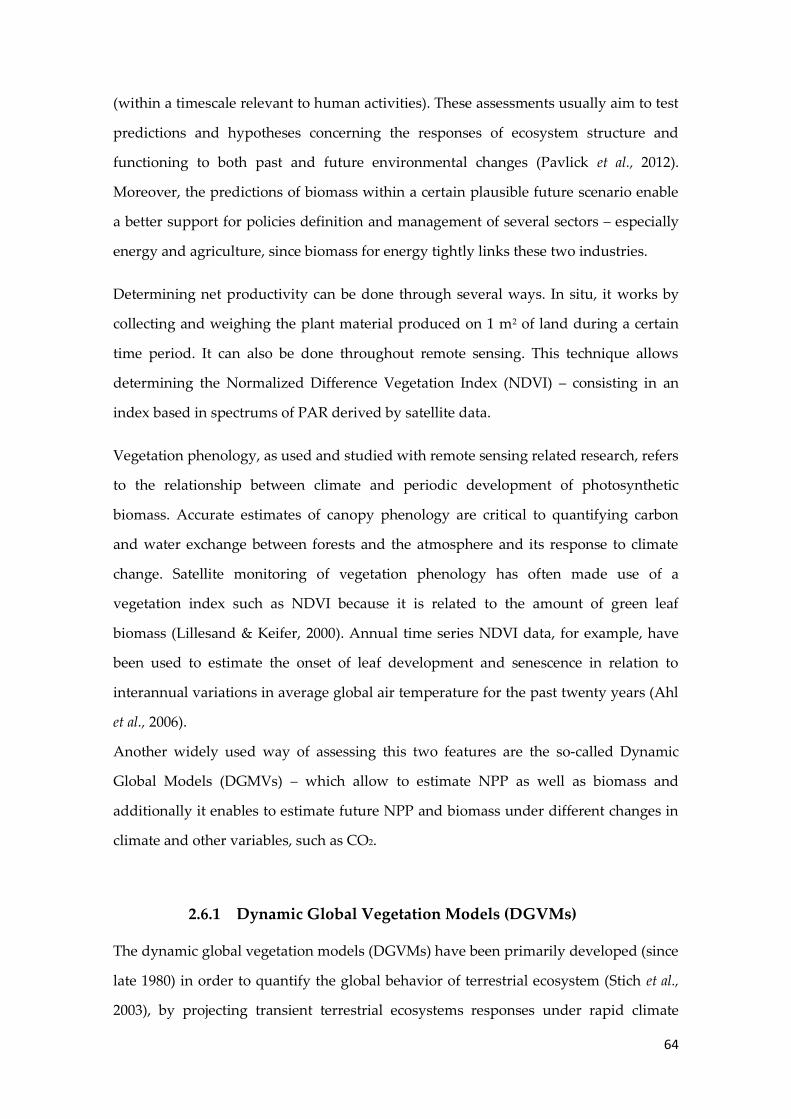
64

(within a timescale relevant to human activities). These assessments usually aim to test

predictions and hypotheses concerning the responses of ecosystem structure and

functioning to both past and future environmental changes (Pavlick et al., 2012).

Moreover, the predictions of biomass within a certain plausible future scenario enable

a better support for policies definition and management of several sectors – especially

energy and agriculture, since biomass for energy tightly links these two industries.

Determining net productivity can be done through several ways. In situ, it works by

collecting and weighing the plant material produced on 1 m2 of land during a certain

time period. It can also be done throughout remote sensing. This technique allows

determining the Normalized Difference Vegetation Index (NDVI) – consisting in an

index based in spectrums of PAR derived by satellite data.

Vegetation phenology, as used and studied with remote sensing related research, refers

to the relationship between climate and periodic development of photosynthetic

biomass. Accurate estimates of canopy phenology are critical to quantifying carbon

and water exchange between forests and the atmosphere and its response to climate

change. Satellite monitoring of vegetation phenology has often made use of a

vegetation index such as NDVI because it is related to the amount of green leaf

biomass (Lillesand & Keifer, 2000). Annual time series NDVI data, for example, have

been used to estimate the onset of leaf development and senescence in relation to

interannual variations in average global air temperature for the past twenty years (Ahl

et al., 2006).

Another widely used way of assessing this two features are the so-called Dynamic

Global Models (DGMVs) – which allow to estimate NPP as well as biomass and

additionally it enables to estimate future NPP and biomass under different changes in

climate and other variables, such as CO2.

2.6.1 Dynamic Global Vegetation Models (DGVMs)

The dynamic global vegetation models (DGVMs) have been primarily developed (since

late 1980) in order to quantify the global behavior of terrestrial ecosystem (Stich et al.,

2003), by projecting transient terrestrial ecosystems responses under rapid climate

http://www.sciencedirect.com/science/article/pii/S003442570600188X#bib15

65

change (Cramer et al., 2001; Pavlick et al., 2012). These models allow the combination of

both biogeochemical processes and vegetation dynamic structures and composition

(and hence changes in ecosystem geography) (Cramer al., 2001; Sitch et al. 2003) and

they have been widely applied to problems regarding global carbon cycle and climate

change.

The DVGM consist of mechanistic, process-based, numerical models, which enable the

simulation at the large-scale dynamics of terrestrial ecosystems (Pavlick et al., 2012).

They simulate the vegetation structure (i.e. distribution, physiognomy) and linked

changes in ecosystem function such as water, energy and carbon exchange, in response

to a scenario of changes in CO2 concentration and climate obtained with the coupled

atmosphere-ocean general circulation models(Cramer et al., 2001).

Soil texture as well as vegetation biophysical processes will affect soil hydrology that

influences the behavior of plant (e.g. its physiology and phenology) and soil (e.g. its

respiration as well as nitrogen mineralization (Cramer et al., 2001). For that reason, the

DGVM include physiological, biophysical and biogeochemical processes, through

mechanistic representations of photosynthesis, respiration and canopy energy balance,

the controls of stomatal conductance and canopy boundary-layer conductance, as well

as the allocation of carbon and nitrogen within the plant (Cramer et al., 2001). Hence,

DGVMs are inclusively embedded within comprehensive Earth System Models (ESMs)

allowing capturing biogeochemical and biogeophysical feedbacks between the

terrestrial biosphere and the physical climate system (Pavlick et al., 2012).

However, each model gives a specific attention to certain processes, i.e. emphasis a

particular detailed description of a process (e.g. plant physiological process including

coupled atmosphere-biosphere model (Cramer et al., 2001). The several existing models

present different complexities as well as different suitability for certain functionalities

(Cramer et al, 2001). In fact, Cramer et al. (2001), have made a parallel evaluation on six

different models (HYBRID, IBIS, SDGVM, TRIFFID, VECODE and LPJ), in order to

point out significant variations between each one in order to represent potential

sources of uncertainty. Moreover, according to Stich et al. (2008), the comparison

66

between several studies results based on DGVMs usually present a wide divergence

between the results regarding the terrestrial biosphere and its function as a driver of

the global carbon cycle under different assumed climate change scenario. The main

uncertainty is mainly the response of the terrestrial carbon balance. Hence, it is fair to

say that each DGVM, has a different degree of complexity and suitability for specific

tasks. It should be taking into account that one of the possible reasons for the

considerable existing divergences may be due to the course of each model or even to a

different plant functional diversity (Stich et al., 2008; Pavlick et al., 2012). The following

sections provide general information about three widely used DGVMs

The figure below (Figure 15) shows the development of a DGVM for a visual (a clearer)

interpretation of it. As it is shown, the DGVMs integrate four main groups of

processes: (1) plant geography, (2) biogeochemistry, (3) biophysics and (4) vegetation

dynamics.

Figure 15 – DGMV scheme (Source: Cramer et al., 2001)

67

Lund-Postdam-Jena (LPJ) Model

The Lund-Postdam-Jena (LPJ) Model, is considered of intermediate complexity and it

is suitable for addressing several global issues. A feature that differs LPJ from other

models is an explicit representation of vegetation structure, dynamics and competition

between PFT population as well as soil biogeochemistry (Sitch et al., 2003).

LPJ model provides a vegetation dynamic response to specific scenario of climate

change. It has an individual-level scale process to the grid cell, where it is employed

biophysical and physiological process parameterizations (as in equilibrium model

BIOME3)(Cramer et al., 2001). Vegetation dynamics are based both on annual net

primary production (ANPP) and biomass growth and include: competition among

PFT; probabilities of natural disturbance (e.g. fire) and succession following

disturbance i.e. replacement of PFT. These processes are simulated explicitly by LPJ


LPJmL was developed in order to simulate two main features: (1) the composition and

distribution of vegetation and (2) stocks and land-atmosphere exchange flows of

carbon and water atmosphere. This model computes processes such as photosynthesis,

plant growth, maintenance and regeneration losses, fire disturbance, soil moisture,

runoff, evapotranspiration, irrigation and vegetation structure through the

combination of ecophysiological relations, generalized empirically established

functions and plant trait parameters (PIK, 2012).

Physiological Principles Predicting Growth (3PG)

The Physiological Principles Predicting Growth (3PG) Model, models the general forest

carbon allocation, published by Landsberg & Waring (1997). The model runs within

simple and readily available input data (e.g. weather records; edaphic variables and

others) and derives monthly estimates of GPP, carbon allocation as well as stand

growth.

The 3PG has also been coupled to satellite imagery of canopy photosynthetic capacity

to model forest growth across landscapes. Similar to other models, 3PG is under

68

constant revision in order to incorporate new research data. In what concerns to its

weaknesses, the allocation and belowground processes are the least developed features

of 3PG. 3PG’s belowground processes.

Jena Scheme for Biosphere –Atmosphere Coupling in Hamburg (JSBACH)

Jena Scheme for Biosphere-Atmosphere Coupling in Hamburg (JSBACH) consists in a

modular land surface scheme which is based on the biosphere model BETHY (Knorr,

2000). It is usually combined with the European Center Hamburg Model 5 (ECHAM5)

soil scheme (Knorr, 2000; Knorr & Kattge, 2005; Thum et al., 2011)enabling the study of

the response of soil organic carbon to climate change, for instance (Thum et al., 2011).

JSBACH enables a better understanding over the feedbacks between the physical

climate system and land surface processes, since it provides a better understanding of

processes that lead to major changes of wither regional or global climates. It bases in

present (or recent past) climate system, allowing thus to comprehend the coupled

climate system.

2.6.2 Main pitfalls and differences between DGVMs

The degree of processes’ complexity also varies among each model Cramer et al., 2001).

One of the several pitfalls of DGVMs, could be pointed out as to be the inexistence of

spatially treatment of seeds dispersal since in accordance with Cramer et al. (2001) the

migration of dominant plants species involves the development of mature individuals

producing seeds besides merely dispersal. Hence, this development would imply

additional delays due to growth and competition processes, since the lack of these

factors on vegetation dynamics, may cause lags of a century or more in the response of

vegetation to climate change, since the results presented are considering stand

development without dispersal.

Another considerable pitfall is the no inclusion of increased nitrogen deposition

(resulting from industrial and agricultural activity) in the DGVM. This lack is

considerable important, since the impacts caused by nitrogen are potentially important

69

to the carbon cycle through changes in plant nutrient availability. Furthermore, it will

also contribute with negative impacts for parallel changes in tropospheric ozone


Despite the uncertainties as well as different complexities and functionalities that

characterizes each model, all of them treat vegetation cover as a fractional

representation consisting of different types (Cramer et al., 2001) the so-called Plant

Functional Types (PFT).

71

3. Methodology to Estimate Productivity and Biomass

Potential under Climate Change

The present goals were addressed by the carbon cycle model JSBACH (Jena Scheme for

Biosphere-Atmosphere Coupling in Hamburg) which ran upon the input data

provided by the climate model ECHAM5 (European Center-Hamburg-Model 5).

JSBACH was expected to provide valuable results regarding the response of terrestrial

productivity and carbon uptake to climate variables change. This carbon model

enabled thus to model how a range of climatic conditions would affect the bioclimatic

areas present in the study area, and therefore, to estimate how their productivity rates

could change in response to a changing climate and atmospheric CO2 concentration - as

well as to understand how significant is the difference of response onto given different

levels of CO2 concentration. Ultimately the results treatment is expected to drive an

understanding of the reliability and value of that model when downscaling the results

at the scale of the Iberian Peninsula, and to comprehend its major limitations.

3.1.Study Area: the Iberian Peninsula

The study area covers the Iberian Peninsula (hereafter IP), the Balearic Islands and a

small portion of North Africa, although a big emphasis was made upon the IP. The

Iberian Peninsula is located in the western-most mainland Europe and it comprises

three nations: Portugal, Andorra and Gibraltar with an area of ~580.000 km2. The

biggest of them, Spain, borders Portugal to the west and to the south of the region of

Galicia. To the south it borders Gibraltar and to the northeast, along the Pyrenees

72

mountain range it borders France and the small principality of Andorra. The south and

eastern continental shelves are bathed by the Mediterranean Sea, whereas the northern

and western continental region it is bordered by the Atlantic Ocean. Figure 16,

illustrates the main regions in which the IP territory is divided as well as the

topographic scheme.

Figure 16 – Map of the Iberian Peninsula – the darker brown is assigned to heights over 1000m; light

brown is assigned to heights ranging between 500 and 1000m (i.e. high plateaus) and the greenish color

are assigned to heights lower than 500m (Source: Solarnavigator.net)

The most common orographic feature prevailing in the IP is high plateaus, which are

divided by the Central Mountain System, into Northern and Southern Plateaus. These

plateaus are isolated from the sea by the so-called Cantabria Mountains in the north

and by the Baetic Mountains at the south. The Iberian Mountain System covers the

north-eastern area and it is parallel to the Ebro River which flowing to Mediterranean

Sea (whereas the remaining rivers flow to the Atlantic Ocean).

In what concerns the flora pattern, the Iberian Peninsula presents a mosaic of forests

except in the most extreme habitats (e.g. alpine environments and arid zones in the

73

Southeast of the Peninsula where conditions struggle a proper tree growth and

survival). Furthermore, human disturbance greatly contributes to unforested areas

since the Neolithic (Blanco et al., 1998).

3.1.1. Bioclimatic patterns and zones

The bioclimatic zones enable to depict the distribution of species across the area

(Guisan & Zimmermann, 2000). Hence, the Iberian territory could be distributed in

several “zones” – which can vary depending on author. For example, the Köpen

classification accounts with five main zones (subdivided in turn in other divisions),

and it is based as well on five vegetation groups (as it is shown in Figure 17) (Kottek et

al., 2006). In order to identify different climates, this climate classification system define

them using average monthly values for precipitation and air temperature, based on

their influence on the distribution of vegetation and human activity (Essenwanger,

2001).

Figure 17- Köppen-Geiger Climate Classification for the Iberian Peninsula and the Balearic Islands (Source: AEMET, 2000)

74

Hence, the Iberian Peninsula, due to its geographical and orographic conditions,

crosses three main types of climates: the “Mediterranean climate” which is the

dominant and comprises two varieties (Csa and Csb); the “Oceanic climate” (named as

Cfb); and the “Semiarid climate” (comprising the varieties Bsh and Bsk)(Kottek et al.,

2006; AEMET, 2011).

Even though that this Köppen-Geiger Climate Classification was created roughly 100

years ago (Kottek et al., 2006), it continues to be one of the most widely used for climate

studies purposes (AEMET, 2011). Table 23 provides a wider description of the varieties

of climate present in the IP.

Table 23 - Iberian Peninsula Bioclimatic zones - In accordance with Rivas-Martínez et al. (2004)

Type Sub-type Main characteristics and locations

B

Arid and

Semi-arid

(Dry)

Climates

P=20(T+7):

P=20 T

P=20(T+14):

BWk* - Hot desert

climate

Or “Hot Desert” and “Cold Desert”. Small areas in the SW of IP.

Spanish provinces of Almeria, Murica and Alicate, coinciding

with minimum rainfall values for the IP. BWh* - Cold desert

climate

Bsh* - Warm semi-arid

climate.

Or “Hot steppe” and “Cold steppe”. Southeast of IP and Ebro

Valley, less in the southern central plateau region, Extremadura

and the Balearic Islands. In Portugal they cover only a small

region of Baixo Alentejo, in the district of Beja Bsk* - Cold semi-arid

climate

C

Temperate

Climates

0˚C

<ATC<18˚C

Csa* - Warm

Mediterranean climate.

Temperate with dry or hot summer. Occupies ~40% of IP area,

southern central coastal region

Csb* - Temperate

Mediterranean climate.

Temperate with dry or temperature summer. NE of the IP ad

west cost of Mainland Portugal and mountainous regions within

the IP

Cfa – Warm oceanic

climate.

Or “humid subtropical climate”. Temperate with dry season and

hot summer. NE of the IP, area of medium altitude surrounding

the Pyrenees

Cfb* - Temperate

oceanic climate.

Temperate with a dry season and temperate summer Cantabrian

Mountain, in Iberian M.R. Pyrenees

D

Cold

Climates

ATC < 0˚C

ATH>10˚C

Dsb – Temperate

continental climate.

Or “Mediterranean continental climate”. Cold with temperature

and dry summer Small areas of the mountains regions at higher

altitudes in the Cantabrian, Iberian and Central M.R. and Sierra

Nevada.

Dsc – Cold continental

climate

Cold with dry and fresh summer. Cold with temperature and

dry summer Small areas of the mountains regions at higher

altitudes in the Cantabrian, Iberian and Central Mountain

Ranges and Sierra Nevada.

E

Polar

Climates

ATH< 0˚C

ET – Tundra Small areas at high altitudes in mountainous regions (Central

Pyrenees and Cantabrian M.R.

ATC – average temperature in coldest month; ATH – average temperature in hottest month; * - Main climates

75

Although, one of the most common and simplest bioclimatic divisions is made in two

macro bioclimatic areas: the Mediterranean zone which occupies a large area of the

centre and south of the peninsula and the Temperate zone, occupying mainly the

northern area (Rivas-Martínez et al., 2004)(Figure 18). The latter has colder

temperatures and higher precipitation than the Mediterranean zone.

Conversely to the Atlantic region, the climate existing in the Mediterranean region is

greatly characterized by a long period of summer drought (commonly lasting between

two to four months). Rainfall can range from 1500 mm to less than 350mm, and

temperatures are widely varying from regions where there is no frost to regions where

winter temperatures drop further than -20ºC. Figure 19 illustrates the mean

precipitation and

temperature of

both zones along

the year:

Figure 19 - Monthly

mean precipitation

and temperature of

temperate zone (left)

and Mediterranean

zone (right)

Figure 18 -Iberian Peninsula Bioclimatic zones - In accordance with Rivas-Martìnez et

al. (2004)

76

3.1.2. Vegetation Cover

In the Atlantic zone, the forests are composed mainly by deciduous trees, more

specifically by oak forests (followed by beech, birch and fir) (Lindner et al., 2008). The

main species account with the Quercus petraea (Sessile oaks), Quercus robur (English

oaks), Fraxinus excelsior (European Ash), hazels, birches (more specifically Betula

species) and Abies alba (Siver Firs) in the Pyrenees , although for higher altitudes, the fir

forests are replaced by Pinus uncinata (the Black Pine). Due to a bit of Mediterranean

influence throughout the area, the presence of Quercus ilex (Holm Oaks) with laurel is

very common. The north Castilla inland sand dunes of the Iberian plateaus host

dominantly stone pine and maritime pine (Pinus pinea and Pinus pinaster, respectively)

(Bacaria et al., 1999; Bohn & Hettwer, 2000) and consist in a very valuable source in

what concerns within a socio-economic perspective as well as a conservation point of

view (Regato-Pajares, 2004)..

The region that occupies the rest of the Iberian territory, i.e. Mediterranean region is

mainly characterized by broadleaf evergreen trees, (as well as thermophilous

deciduous forest; xerophytes coniferous forest; plantations and self shown exotic

forest)(Lindner et al., 2008). Within the shift from the Mediterranean vegetation to the

Atlantic vegetation, the Quercus pyrenaica (also known as Pyrenean Oak) stands as a

great importance in what concerns the widen area covered in the Iberian Peninsula.

The resistance of this oak enables it to prosper along the mountain ranges in the centre

of the Peninsula, as well as along the interior of Galicia to the south of the Cantabrian

Cordillera and throughout the Central System reaching inclusively the south – Sierra

Nevada and Cádiz. The main forests in Mediterranean forests are oak forests (where

Quercus ilex is common), cork oaks, wild olives or juniper (to name few). The Pinus

halepensis (or Aleppo Pine) is responsible for replace these trees in the warmer regions.

For the areas characterized by sandy ground, forest of Stone Pine and juniper enable

the sand dunes fixing.

The Central plateaus, valleys and low plains of the interior portion of the IP are mainly

covered by sclerophyllous and semi-deciduous forests. Due to their more continental

climate, the northern plateau was primarily evergreen broadleaf and conifer canopy

77

species, but to several degradation factors, it has currently turned into secondary,

dense shrub land, or into agro-forestry landscapes mainly constituted by scattered

trees on grasslands or crops. In the western part of the region, mixed cork oak (Quercus

suber) and holm oak sylvopastoral woodlands are frequent.

The southeastern part of the IP, along with the Ebro valley, is covered by woodlands of

juniper(Juniperus thurifera, J. phoenicea), Aleppo pine (Pinus halepensis) and holly oak

(Quercus coccifera) mixed forests. These forests and woodlands alternate though with

extensive steppe grasslands (such as Stipa tenacissima, Lygeum spartium and shrub

communities (Artemisia herba-alba, Thymelaea hirsuta, Ononistridentata, Helianthemum

squamatum, Thymus mastigophorus) resulting thus in a complex mosaic-like landscape

(Bacaria et al., 1999; Bohn & Hettwer, 2000).The southern part of the region and the

river canyons of the Douro and Tejo river have a wide distribution of wild olive (Olea

europaea) and carob (Ceratonia siliqua) woodlands as well as maquis – this plants have

been strongly domesticated in order to produce food crops and olive oil.

In what concerns the herbaceous species (such as Arisarum vulgare, Vinca difformis,

Allium triquetrum, and Ballota hispanica ), those also frequently appear within the dense

and shady tree layer. A wide range of the vegetated regions have been widely and

intensively transformed into agricultural land of extensive wheat crops, vineyards,

almond and olive groves, fruit tree orchards and other irrigated crops (Bacaria et al.,

1999; Bohn & Hettwer, 2000). Hence, the southwestern part of the region is highly

characterized by manmade, semi-natural sylvopastoral woodlands known as

“montados” in Portugal or “dehesas” in Spain (Regato-Pajares, 2004).

3.1.3. Climate Vulnerability

The IP presents high climate vulnerability caused b its peculiar complex environment

and location in the transition area between subtropical and temperate climates (IPCC,

2007; Jerez et al., 2012). In this context, vulnerability is defined as the degree to which

the IP is susceptible to be affected by adverse effects of climate change. Under a climate

change scenario, the climate fragility of the IP is altered and there are evidences of

observed and predicted increases of temperature and decreases in projected

78

precipitation (IPCC, 2007). For the Temperate zone, annual mean temperature

increases are projected to drive extreme and more frequent events are (such as floods,

and higher volumes and intensities of precipitation in winter), whereas The

Mediterranean zone is projected suffer droughts as result from forecasted decrease in

annual precipitation (Lindner et al., 2008). The table below shows some an overall

assessment of the IP bioclimatic regions under a bio-geographical perspective (Table

24):

Table 24 – Sensitivity of Bioclimatic zones: expected climate change and potential impacts (Source:

Adapted from Lindner et al. (2008))

TEMPERATE OCEANIC ZONE

Expected climate

change

Temperature increase +2.5 - +3.5°C (by the end of the century;

Hotter and dryer summers;

More frequent extreme events;

Higher volumes and intensities of precipitation in winter

Potential impacts

and key treats

Tree growth rates may increase but also decrease in water limited areas

Extreme events such as storms, droughts, flooding, and heat waves

Risk and frequency of wind damage increase

Shifting natural species distribution ranges may negatively impact

especially rare species living in isolated habitats

Biotic pests are expected to have increased damage potential

MEDITERRANEAN ZONE

Expected climate

change

Temperature increases +3 - +4 °C, larger increases during the summer

(+4 - +5 °C) and smaller increase in winter

Annual rainfall is expected to decline up to 20% with even stronger reduction in

summer

Precipitation increase in winter

Extreme events such as heat waves and heavy precipitation events more frequent

Potential impacts

and key treats

The extreme forest fire risk

Tree growth is expected to decline in large areas due to more severe

drought limitations

Increasing drought limitations are threatening the survival of many species

One of the most concerning consequences is the fact that these changes can be

responsible for worsening the drought conditions c leading to aggravated water-

scarcity conditions(IPCC, 2007). Making it necessary to estimate and predict the

temporal variability of meteorological drought events over the IP, in order to project

the severity of dry and wet conditions over 30 years-mean period.

Some major signs which support the latter concerns were found in summer season

which in accordance with some studies (e.g. Jerez et al., 2012) have been showing a

strengthening in the increase projected for both mean temperature and temperature

79

variability as a consequence of soil moisture-temperature feedback. Thus, such

influence of the land-surface processes – such as the soil moisture, draws a growing

attention and need of wider assessments, when projecting the future changes for

temperature, precipitation and wind over a complex are as the IP.

Parallel to this phenomenon of warming temperatures, the decrease in precipitation,

soil moisture and evapotranspiration draw great concerns about vegetation

productivity over the IP, since that in most of the IP territory (mainly the

Mediterranean zone) the vegetation is water-limited(Rios-Enteza & Miguez-Macho,

2010, Jung et al. (2011). Most of the tree species under climate change vulnerability are

mainly affected by drought (such as the Eucalyptus spp, Pinus spp and oaks).

3.2.Modeling Tool: JSBACH

The goals stated for this work, were achieved by handling data results yielded

by the JSBACH model which were processed by Christian Beer (Max-Planck-

Institut für Meteorologie Hamburg (MPIBGC)) and post processed by Nuno

Carvalhais (MPIBGC and Faculty of Sciences and Technology of New

University of Lisbon (FCT-UNL)). This section addresses a more detailed

description of the model along with the variables analyzed and data input

sources.

3.2.1. JSBACH overall description

JSBACH consists in a modular land surface scheme. It enables to understand the

interaction between the assimilation rate and stomatal conductance, which are

explicitly modeled and dependent on temperature, soil moisture, water vapor,

absorption of solar visible radiation as well as ambient CO2 concentration (Raddatz et

al., 2007). The vegetation phenology is driven by temperature, soil moisture and NPP.

JSBACH aims to model land carbon fluxes throughout biologically control and

therefore, other natural processes such as fires, leaching or weathering (Thum et al.,

2011) nutrient limitations (Raddatz et al., 2007) and competition among plants derived

80

by climate change are not encompassed by the model. The carbon balance regards

hence the cycle of carbon storage along the growth and death of the plant, and the

model also accounts with anthropogenic impact on the land carbon cycle through land

cover maps (Thum et al., 2011).

JSBACH runs having as input data basis a global climate model (GCM), named as

ECAHM developed by the Max Plank Institute (MPI) for Meteorology. More

specifically, the ECHAM5 consists in an atmosphere/ocean general circulation model

(AOGCM) and was created upon the modification of a previously developed global

forecast model by the European Centre for Medium-Range Weather Forecasts

(ECMWF) (Raddatz et al., 2007). The interaction between JSBACH and ECHAM is

multilateral and encompasses many parameters. For a clear interpretation of the

coupled models setup, an illustrative overview is presented below (

).

The JSBACH climate components include atmosphere-biosphere interactions as well as

soil-biosphere and land-atmosphere

interactions (Brovkin et al., 2009; Reick,

2009). The boundary land-atmosphere poses

on many features which are directly affected

by the presence of vegetation: such as CO2

exchange; surface roughness, albedo and

surface temperature, as well as

evapotranspiration and heat latent flux

(Reick, 2009). As a technically modular

framework, JSBACH model contains the

following components:

Land surface scheme – in order to

describe soil heat and moisture interactions;

Figure 20 - Interactions between JSBACH and

ECHAM5

81

Fast vegetation processes – which derive carbon fluxes from photosynthesis in

diurnal cycle embedded in the full land surface energy balance, accounting for

plant phonological changes and respiration;

Slow vegetation processes – which provide the description of long-term

interaction between climate and vegetation.

JSBACH Modules

The estimations and modeled processes that JSBACH perform are possible since they

are based on many other models – or modules (Figure 21). I.e., in what concerns to the

vegetation processes, for the fast processes JSBACH is based on the BETHY scheme (or

“stomata model”), which holds a description of photosynthesis embedded in the full

land surface energy ecosystem balance as well as plant respiration and phenology

scheme (Knorr, 2003; Thum et al., 2011). Moreover, the actual soil carbon module used

is called CBALANCE

(or “carbon flow

model”), which in fact

consists in the original

soil carbon ever used

for JSBACH (Thum et

al., 2011).

Besides the stomata and the carbon flow models (which will be addressed more closely

afterwards), JSBACH also encompasses the phenology model (related to the Leaf Index

Area (LAI)); the dynamic land cover; and the soil model: ECHAM5. The later regards

surface and soil hydrology; energy balance and mosaic approach for surface properties

.The dynamic land cover concerns the determination of the type of vegetation cover.

Figure 21 - JSBACH

modules scheme

82

3.2.2. BETHY module: Plant Functional Types (PFTs)

Generally speaking, the BETHY model is responsible for simulating the water cycle

throughout transpiration (i.e. assessing the stomatal conductance sensitivity to CO2 in

ambient air) and for the carbon cycle throughout the photosynthesis process, i.e. NPP

or carbon assimilation (Knorr & Kattge, 2005; Raddatz et al., 2007Reick, 2009).

BETHY scheme simulates coupled photosynthesis and energy balance processes

throughout simulations of the CO2, water and energy exchanges between the

atmosphere and plant canopy and it also computes absorption of PAR as well as the

response of canopy conductance to PAR (Knorr & Kattge, 2005; Raddatz et al., 2007).

Moreover, the BETHY model enables the calculation of evapotranspiration and heat

fluxes (Monteith, 1965). Some of the processes are computed upon many other authors,

listed in the Table 25.

Table 25- BETHY processes

Parameters Source

Transpiration Penman-Monteith equation by Monteith, 1965

Sensible heat fluxes

Carbon uptake for C3 plants Model by Farquhar et al. (1980) GPP

Carbon uptake for C4 plants Model by Collatz et al., (1992)

Stomata and canopy model Canopy simulation in response to PAR by Knorr

(2000)

The model parameters are: photosynthesis, carbon balance, stomatal control as well as

energy and radiation balance. The GPP estimations are provided throughout C3 and

C4 photosynthesis and stomatal conductance processes; plant respiration is throughout

growth respiration (~NPP) and maintenance respiration; soil respiration is throughout

fast/slow pool response, temperature and moisture balance and finally, carbon balance,

is simulated throughout average NPP at each grid point (Knorr, 2000).

83

Hence, the BETHY scheme (Figure 22)

confers one of the main features that

actually characterize JSBACH approach to

production estimations: the fact that these

are made, following an up scaling

approach, i.e. from leaf to canopy. The Fact

Box S below shows the processes. These

processes and fluxes occurred at the level

of each specific Plant Functional Types

existing in the 0,5˚ x 0,5˚ grid cell deployed

over the European region.

BOX: S Scaling production from leaf to canopy (Source: Reick,

2009)

Having A as assimilation; Rd as dark respiration; Rg as growth

respiration; Rg as maintenance respiration; Rh as heterotrophic (soil)

respiration and LAI as leaf area index, hence:

From photosynthesis: ( ( ) ( ))

Gross primary

productivity: ( ( ) ( )

Net primary productivity: –

Maintenance respiration: ∫

Construction costs:

(5 C are needed to allocate 4C)

( ) * | +

and

Net Ecosystem Exchange (NEE):

Figure 22 –BETHY scheme

84

Plant Functional Types (PFT) in JSBACH

In JSBACH, the vegetation (which allocated in a grid cell) is described in terms of

different Plant Functional Types (PFTs) (Sitch et al., 2003). PFTs symbolize broad

phonological, biogeographically and morphological aggregations within every

parameter value is held temporally and spatially constant and responses to physical

and biotic factors are assumed to be similar (Prentice et al., 2007). They enable thus, to

account generally the variety of structure and function among plants (e.g. woody such

as tropical, temperate and boreal; herbaceous) (Sitch et al., 2003), by aggregating the

biogeochemical fluxes and vegetation

properties within each grid cell (Pavlick et al.,

2012). For that reason the average of a PFT

consists in the fundamental entity simulated

in JSBACH since this concept enables to

deploy the processes run at the level of the

plants individually within their PFT which

will ultimately scaled up to the “population” over the grid-cell (Figure 23).

PFT are a main feature in a DGVM mainly due to two reasons. Firstly, to each PFT a set

of parameterizations is assigned, concerning the ecosystem processes (such as (1)

phenology; (2)leaf thickness; (3) minimum stomatal conductance; (4) photosynthetic

pathway; (5) carboxylation rate; (6) maximum electron transport rate; (7) specific leaf

area carbon content, and (8) phenotype, to name few) (Cramer et al., 2001; Raddatz et

al., 2007), and thus the segregation of vegetation in groups assigned to range of similar

behavior regarding responses to environmental conditions enables a simplification of

the existing plant complexity. Moreover, it is also very useful for modeling in a

mapping context such as when applying the DVGM (Lavorel et al., 2007). Secondly, the

structural characteristics of the vegetation can be defined by the representation of

different PFTs at a certain point in time and space (Cramer et al., 2001; Lavorel et al.,

2007) which will ultimately enable the monitoring effects of global change or

management on vegetation distribution and ecosystem processes (Lavorell et al., 2007).

Figure 23 - Gridl cell example

85

It is important to notice that the classification applied to each PFT, depends on the

ability of association between vegetation traits and function on model (see Figure 24

for examples) and ultimately it depends on the objectives of the modeling purpose.

Figure 24 - Examples of soft traits and associated functions (Source: Canadell et al., 2007)

In fact, some authors have categorized agriculture according to crop functional type

based on management practices (besides phenology and physiological parameters);

while others have performed a hierarchical classification based on response of

vegetation to fire disturbances. Nevertheless, PFT schemes used by DGVMs use to be

criticized for ignoring much of the knowledge about comparative plant ecology

(Harrison et al., 2010). Furthermore, several plant features present a considerable

variation within PFTs and in fact, for many important features that variation can even

become greater within PFT rather that between different PFT (Pavlick, et al., 2012 ).

The grid cell simulation runs after the insertion of input data which includes seasonal

(e.g. daily time scales) climatology; soil type and atmospheric CO2 concentration which

driven daily potential evapotranspiration and monthly soil temperatures. Thus,

seasonal course of leaf phenology is calculated for each PFTs (Sitch et al., 2003). The

obtained results allow illustrating (within one particular scenario of atmospheric

composition and climate change), the range of responses of state-of-the-art terrestrial

biosphere models (Cramer et al., 2001).

86

Each model grid cell is divided into tiles, and then, the surface condition and fluxes are

calculated separately for each tile – which holds a single PFT. Afterwards, the grid cell

average is given to the atmosphere (Figure 25).

Figure 25 - The tilling approach (Source: Adapted from Brovnik et al., 2009)

Summing up, the vegetation was described in a grid cell of different PFT, based on

attributes which control the physiology and dynamics to which each PFT was

assigned. Within this model 21 PFT were defined, as listed in the Table 26.

87

Table 26 - Plant Functional Types considered by JSBACH

No. PFT Biomass type

1 Glacier -

2 Tropical evergreen trees “Forest” Biomass

3 Tropical deciduous trees “Forest” Biomass

4 Extra-tropical evergreen trees “Forest” Biomass

5 Extra-tropical deciduous trees “Forest” Biomass

6 Temperate broadleaf evergreen trees “Forest” Biomass

7 Temperate broadleaf deciduous trees “Forest” Biomass

8 Coniferous evergreen trees “Forest” Biomass

9 Coniferous deciduous trees “Forest” Biomass

10 Rain green shrubs “Forest” Biomass

11 Deciduous shrubs “Forest” Biomass

12 C3 grass “Herbaceous” Biomass

13 C3 grass “Herbaceous” Biomass

14 Pasture “Herbaceous” Biomass

15 C3 Pasture “Herbaceous” Biomass

16 C4 Pasture “Herbaceous” Biomass

17 Tundra -

18 Swamp -

19 Crops “Herbaceous” Biomass

20 C3 crop “Herbaceous” Biomass

21 C4 crop “Herbaceous” Biomass

The cover types of PFT for each one of four tiles existing in each grid cell, is presented

in Figure 26 since the discrimination of vegetation type distribution might be useful for

further interpretation of output data. (As explained before, the spatial distribution of

PFT across the Iberian Peninsula is constant along the time, since JSBACH does not

assume land use dynamics. Additionally for simplification matters, the results were

aggregated in three main groups: (1) “Forest biomass “which includes the PFT listed

from 2 to 11 (and hence trees and shrubs were accounted together); (2)“Herbaceous

biomass”, which comprises the rest of PFT excluding glacier, swamps and tundra and

88

(3)”All” - which regards all PFT together. Table 27 depicts some of the species that are

found in IP, assigned to the major PFT from forest biomass :

Table 27- Major species existing in Iberian Peninsula assigned to forest type (Source: Alcaraz et al.,

2006)

PLANT FUNCTIONAL TYPE SPECIES IN IBERIAN PENINSULA

Coniferous evergreen trees Pine (Pinus spp), junipers (Abies spp), firs and spruces (Picea spp)

Temperate broadleaf trees ; Quercus suber; Quercus ilex; Quercus petraea; Quercus cerris;

Eucalyptus globulus; Populus; Fagus sylvatica

Temperate Broadleaf deciduous trees Castanea sativa

In Appendix A it can be found further information regarding the most common crops

existing in the Iberian Peninsula, along with their spatial distribution.

89

Figure 26- Cover Type per tile

90

3.2.3. CBALANCE module

The CBALANCE module regards the heterotrophic respiration (from soil), the net CO2

exchange with atmosphere (NEP) and it also accounts with carbon in plants and soil

pools, the so-called C-pools . Throughout this model, JSBACH simulates the carbon

flow, more specifically the storage of carbon on land within five “pools” which are

measured in mole of carbon per square meter (mol(C)/m2(canopy)) – translating thus in

carbon density per square meter of canopy. However, only some of them (three, in fact)

are regarded in this dissertation, namely the “Green pool”, the “Wood pool” and the

“Reserve pool” – which consists of the state variables of the model (Reick, 2009).

The segregation of carbon pool is made upon the rate of carbon storage which is

different from tissue to tissue within the same plant (Figure 27). The green pool is

composed by the living parts of plants such as the leaves, the fine roots and sapwood

and does not take into account reserves. The reserve pool is hence composed by sugar

and starches that plants store as an energy reserve. Finally, the wood pool consists of

the woody part of the plants, comprising thereby the stems, the branches and the roots.

Figure 27 - Scheme of different Carbon pools for different PFTs

The green and reserve pools have a higher rate of carbon intake compared to wood

pools, which are hence slower carbon pools. Thus, the JSBACH model simulates the

growth of vegetation assuming certain percentage values of NPP assigned to each the

pool composing each PFT in different percentages.

Figure 28 provides an illustrative interpretation of this explanation.

91

Figure 28 - CBALCANCE Carbon Pool model

The calculated NPP (from BETHY module) is hence assigned to the three carbon pools.

Each vegetation carbon pool will afterwards be assigned to other soil carbon pools: fast

or slow soil pool (as it is shown in

Figure 28) which is dependent on carbon pool, soil humidity surface temperature and

time. Finally, these two soil carbon pools will contribute with carbon release onto the

atmosphere, i.e., soil respiration (Reick, 2009). Therefore, the input data for

CBALANCE model consists of NPP; LAI; soil moisture and temperature (Reick, 2009).

92

3.3.Model variables: inputs and outputs

The input data of JSBACH model (consisting in the mean annual climatology) used for

this work is composed by six variables listed in Table 28, upon which the simulation in

every single cell will be driven by – as illustrated in Figure 25:

Table 28 – Climate input variables

No. Variable Time

1 Air temperature at 2m above ground 30 min.

2 Downwards long-wave (infra-red) radiation flux 30 min.

3 Downwards short-wave (solar) radiation flux 30 min.

4 Precipitation (Rainfall) 30 min.

5 Specific humidity at 2m above ground 30 min.

6 Wind speed at 10m above ground 30 min.

The relevant output for this dissertation include: Gross Primary Productivity; Net

Primary Productivity and Biomass.

3.4.Model datasets

The complete data set that composes the scheme supporting JSBACH, consisted of a

fusion between the data sets provided by the Water and Global Change (WATCH)

project and by the ERA INTERIM. The conjunction of both datasets comprises the

climatic parameters which will be used as input data enabling thus to run the JSBACH.

The nature of both data sets regards some attention, since a considerable part of

JSBACH results reliability is dependent of the accuracy of forecasted results.

3.4.1. WATCH data sets

The Water and Global Change (WATCH) Project (which consisted in an Integrated

Project funded under the Sixth Framework Program of European Union) gathers data

regarding the components of current and future global water cycles as well as water

resources states – for the recent past and the future. In short, the WATCH program

provides an extensive analysis of the global water resources it also evaluates their

93

uncertainties and overall vulnerability of global water resources related to the main

societal and economic sectors (Harding et al., 2011).

WATCH was developed after having a consistent set of climate data input throughout

an acquired understanding of water cycle in recent past. Therefore, the WACTH

project comprises two different data set regarding past climate scenarios and predicted

climate/hydrological scenarios, namely, “WATCH Forcing Data” and “WATCH

Driving Data”, respectively.

The “WATCH Forcing data” covers the period 1901-2001 and it is based on a global 0,5

x 0,5 degree (approximately 50x50km) grid and the eight essential climate variables are

comprised within it. These data result from merging observational dataset along the

period; adding further observational procedures and are also subject of local validation

against hourly meteorological data. These data can be hence, be used as input in

several models, such as hydrological models which enable to produce comprehensive

global water cycle data sets.

On the other hand, the “WATCH Driving Data” is covering the period 2001-2100,

composing thus the 21st century data set. This data was created employing a novel bias-

correction methodology which was trained on the 20th century WATCH Forcing Data.

Hence, the WATCH Driving Data provides the same variables as the WATCH Forcing

Data and use the same grid as well. These forecasted applied have been created from

three well-established climate models which are running under two IPCC future

emissions scenarios (Harding et al., 2011). Hence, generally speaking, it evaluates the

terrestrial water cycle throughout the use of land surface models as well as general

hydrological models in order to asses significant variables (such as evaporation, runoff

and soil moisture).

3.4.2. ERA interim data sets

Era-Interim consists in the latest global atmospheric reanalysis developed by the

European Centre for Medium-Range Weather Forecasts (ECMWF). The ERA-Interim

94

project incorporates a forecast model with three fully coupled components for the

atmosphere, land surface and ocean waves. It computes variation analysis of the basic

upper air atmospheric fields (such as temperature, wind, humidity, ozone and surface

pressure) as well as near-surface parameters (such as 2m temperature and 2m

humidity); soil moisture and temperature; snow and ocean waves (Dee et al., 2011).

Similarly to WATCH, ERA-Interim also covers a time period back at the 20th century

(specifically from 1989 onwards) and it is extended forward in near-real time (Dee et

al., 2011). The data is also aggregated in a gridded scheme basis including 3-hourly

surface parameters, although these parameters includes a bit wider range of

parameters natures (e.g., such as the weather; the ocean-wave and land-surface

conditions. The upper-air parameters (which cover both troposphere and stratosphere

are run over a 6-hour scheme (Dee et al., 2011). The forecasted information is possible

through the model equations which enable extrapolating data from observed

parameters, resulting in physically meaningful forecasted results. Reanalysis data

provides a spatially complete and multivariate record of the global atmospheric

circulation, and it is produced with a single version of a data assimilation system

which includes the forecasted model used. This reanalysis provided by ERA-Interim

was produced with a sequential assimilation scheme, advancing forward in time

forward in time using hourly cycles.

JSBACH Storyline

The input data provided by the datasets, was selected according to the SRES scenario

A1B, already mentioned. The A1 family was chosen, since it has the highest rates of

technological change and economic development. Moreover, the trend of the global

population growth is similar to some studies that regard these predictions (i.e. a

growing population which peaks in the mid-century declining afterwards) (IPCC,

2000).

The A1 family and storyline also predicts a future world of rapid economic growth as

well as the rapid introduction of new and more efficient technologies (IPCC; 2007).

Although, the scenario A1B, (also known as the “balanced” scenario), in fact balances

95

across all energy sources. Hence, by being “balanced” means that this scenario does

not rely too heavily on one particular energy source, assuming thus similar

improvements rates applied to all energy supply and end-use technologies. This

scenario, predicts a CO2 increase until around 2050 and then decreasing after that

(Figure 29).

Table 29 depicts some of the main driving forces responsible for the estimations of CO2

emissions presented in the previous figure.

Figure 29 – Global carbon dioxide emissions (Gt(C)/year) for scenarios A1F1, A1R and A1B (IPCC, 2000)

Table 29 - Overview of main driving forces and CO2 emissions across the years for A1B Scenario

(Source: IPCC, 2000)

Future Reference: 1990 A1B Scenarios

Population (billion)

2020

2050

2100

5,3

7,5

8,7

7,1

World GDP (1012

1990US$/yr)

2020

2050

2100

21

56

181

529

Per capita countries

income ratio: Annex-I 12

to Non-Annex-I 13

2020

2050

2100

16,1

6,4

2,8

1,6

CO2 fossil fuels (GtC/yr)

2020

2050

2100

6,0

12,1

16,0

13,1

3.5 Simulation Condition and Scenarios

12

Developed countries and economies in transition 13

Developing countries

96

In order to accomplish the goals set for the present work, four different scenarios were

considered as it is shown in Figure 30. The [1960-1990] period – hereafter also referred

as “Reference Period” consists in a base time period regarding the recent past which

will serve as a comparison period during the assessment of change in climate or carbon

balance projected for future scenarios. Moreover, this reference period also enables to

evaluate the model’s accuracy having recorded data for comparison purposes.

Figure 30 - Reference Period and Future Scenarios considered for the results

For the future prospects, two time periods were considered: covering the period from

2060 to 2090, and from 2070 to 2100. To each time period, two different conditions in

atmospheric CO2 concentration were assumed. The scenarios “C”, namely scenarios C1

(2060-2090) and C2 (2070-2100) assume constant atmospheric CO2 concentrations, i.e.

these scenarios maintain

the same CO2 levels

existing during the

reference period

~296ppm. Conversely, the

scenarios “E” account

with a rise of CO2 levels,

namely of 88% in scenario

E1(2060-2090) and 99% in Figure 31 - Atmospheric CO2 concentrations during the

Reference Period and the Future Scenarios

97

scenario E2 (2070-2100) from reference period (Figure 31). Nevertheless both C and E

scenarios assume the same climate changes.

The climate conditions characterizing the future scenario are in accordance with

JSBACH storyline, (i.e. the A1B SRES scenario) meaning that climate changes are

projected to occur in 2060-2090 and 2070-2100 and that both scenarios “C” and “E” are

under the same changing climate conditions. The only difference (or varying variable)

between “C” and “E” scenarios is thereby the concentration of atmospheric CO2 and

therefore the comparison analysis between a scenario of Constant CO2 and a scenario

of Elevated CO2, enable to assess the solely impact of the CO2 variable on an output

result (Figure 32):

Figure 32 - Assessments from possible comparisons between Scenarios C1, C2, E1, E2 and the Reference

Period

Figure 32 helps to illustrate the information that can be depicted from the comparison

between a pair of scenarios. The comparisons between the output results from different

scenarios (which consist in the variable mean of 30-years period scenario, over the IP)

will be dependent on the information that it is expected to take from it. When it is

aimed to understand the impact of CO2 variation in productivity enhancement or

biomass difference, for instance, the pairs of comparison are scenarios C1 and E1, and

scenarios C2 and E2 (as there is no other variable varying between the scenarios

besides CO2). For realistic approaches, such as the assessment of biomass resource

potential in future energy market, the comparisons rely on the E1 and E2 scenarios, as

they meet the most likely future conditions (i.e. increase of CO2 besides the changing

climate variables).

98

3.6 Data handling and treatment

Data handling concerned the treatment of results regarding both the reference period

and future scenarios: namely the results from climate variables and carbon balance

variables yielded by JSBACH model. Table 30 and Table 31, describes the overall

scheme setup of the work-flow concerning data handing and analysis:

Table 30 - Work flow of the three main stages of data treatment

I –Reference Period: Climate variables* analysis

1 - Quantitative and qualitative analysis of

spatial distribution of each climate variable

during the period [1960-1990];

2 - Spatial and qualitative comparison

between climate patterns;

3 - Assessment of correlation between

spatial distributions of climate variables

variable.

*APAR and SWC are not climate variables

[1960-1990]

Variables under study:

Land surface temperature

Precipitation

Evapotranspiration

Soil moisture

Radiation (PAR and APAR)

II – Reference Period: Carbon balance assessment

1 - Quantitative and qualitative analysis of

spatial distribution of each carbon-related

variable during the period [1960-1990];

2 - Spatial and qualitative comparison

between climate patterns and PFT locations;

3 - Assessment of correlation existing spatial

distribution of GPP and climate variables;

4 - Accounting of total biomass existing

during the Reference period and

discrimination of each PFT contribution;

5 - Assessment of correlation existing spatial

distribution of Biomass and climate variables;

[1960-1990]


GPP

NPP

Biomass (Herbaceous and Forest)

WUE

LUE

99

Table 31- Work flow of the three main stages of data treatment (cont.)

III – Future Scenarios: Climate Change Assessment

1 - Spatial distribution comparison/analysis

of quantitative alterations estimated for

scenarios “C1”, “C2”, “E1”, “E2” and

reference period;

2 - Analysis of differences and the

magnitude of the annual mean changes of

each variable;

3 - Statistical comparison between results

from future scenarios and Comparison of

results with predictions studies made at

global scale or IP scale, within the A1B

scheme.

([2060-2090] & [2070-2100])/ [1960-1990]


Δ Land surface temperature

Δ Precipitation

Δ Evapotranspiration

Δ Soil moisture

Δ Radiation (PAR and APAR)

Climate Changes comparisons:

IV – Future Scenarios: Carbon balance assessment

1 - Spatial distribution comparison/analysis

of quantitative alterations estimated for

scenarios “C1”, “C2”, “E1”, “E2” and

[1960-1990] time aggregation;

2- Comparison of the magnitude of the

annual mean change of change of

variables;

3- Analysis of correlation (between all Δ

climate variable for ΔGPP and ; Forest and

Herbaceous Biomass;

4 -Statistical comparison between scenarios

“Future C” and “Future E” (Δ GPP; ΔNPP

and Δ Biomass

5 – Predictions of biomass energy

potentials (EJ) and analysis in terms of

significance to the current energy system.

([2060-2090] & [2070-2100])/ [1960-1990]


Δ GPP

ΔNPP

Δ Biomass

ΔWUE

ΔLUE

Comparisons between scenarios:

An overall setup of the methodology in regards to data treatment and final results is

illustrated in Figure 33:

100

Figure 33 - Overall Methodology Scheme

101

3.6.1 GIS Analysis

The images created by JSBACH model as arithmetic variables were processed

throughout map algebra operations under a GIS (Geographic Information System) tool

(IDRISI-Taiga), enabling spatial modeling and visualization. In the following section,

selected GIS analyses are presented to illustrate how JSBACH data was handled in a

GIS.

Units Conversion

A major task performed in the GIS refers to units’ conversion. For example, maps for

Mean Surface Temperature units in Kelvin, were converted to maps in degree Celsius.

Hence, as illustrated in the following IDRISI flowchart (Figure 34), a raster image

(having the same spatial parameters than every map) was firstly created with initial

single value set to be “273.15”.

Afterwards, this new map (273map) was combined with the map of Mean Surface

Temperature (in Kelvin) throughout a overlay operation enabling to create another map,

by subtracting to each grid cell from the original map in Kelvin the value of 273,15

(since 1 degree Celsius corresponds to 273,15 degree Kelvin), resulting in a map unit of

degree Celsius.

Figure 34 - Flowchart: creating an image with different units - example for temperature (degrees Kelvin

to degrees Celsius conversion example)

The same procedure was applied for the differente time agreggations, and after

building up the new map. GIS also provide a graphic frequency histogram and

statiscits of the cell values for each image (Eastman, 2009), through the module histo.

The number of classes and widths were defined similarly to each set of parameter, in

order to facilitate visual interpretation and comparisons between eventual changes of

statically distribution.

102

A similar approach was made in order to convert precipitation and evapotranspiration

maps (which units were initially expressed in kg/m2/s – and were converted to

mm/year); as well as GPP; NPP and biomass maps (which was initially expressed in

mol(CO2)/m2. . In some cases, such as soil moisture maps and biomass maps, the overlay

module was also used in order to add or “sum” maps. In the case of soil moisture,

several layers were added creating the final soil moisture map, whereas for the

biomass map, overlay was applied to the three carbon pool of biomass (i.e. wood, green

and reserve).

The overlay operations, also enable to create indexes based on prior maps. For example,

to understand the water productivity over the IP during a certain time period – i.e.

how much biomass would be created for a certain amount of water, the maps

containing the evapotranspiration distribution and the GPP maps were related by

using the division process.

Assessing percentage changes

In order to understand the scale of change between two different scenarios, map

algebra operations (imagediff) were performed as shown in Figure 35, enabling to

compare two quantitative images of the same variable for different dates (Eastman,

2009), to assess the percentage change between each image.

Figure 35 – Procedure to evaluate percentage change of land surface temperature between Temperature

C1 (Scenario C1) and Temperature C2 (Scenario C2)

These procedures were used to assess the difference between a future scenario and the

reference scenario, such as for instance the precipitation maps –which enable hence to

understand “how less mm would rain within a 100 year time difference”.

103

Assessing images ratio changes: GPP example

Another procedure taken to assess changing variables over the time, was throughout

the ratio between the later image (from a future scenario for instance), and the

reference period. Figure 36 is illustrating this procedure as used for the visualization of

overall changes (in terms of “positive” and “negative changes), such as increases or

decreases of GPP over the Iberian Peninsula. This step as used whenever it was needed

an clear visualization of overall changes (in terms of “positive” and “negative”

changes), such increases or decreases of GPP over the Iberian Peninsula.

Figure 36 - Procedure to evaluate ratios GPP between reference period and scenario C1

3.6.2 Statistical Analysis

To evaluate the ecosystem response to climate variability, correlation analysis were

performed between the mean annual carbon variables (i.e. GPP, NPP, forest and

herbaceous biomass) and the mean annual climate variables, i.e. land surface

temperature (T), precipitation (P), evapotranspiration (ET), soil water content (SWC),

PAR and APAR, using data from each scenario. The results (i.e. correlation coefficients

and determination coefficients) enabled to assess the relationship between the

interannual variability in the carbon fluxes and climate variables, as well as the spatial

pattern of pairs of variables during the reference period (e.g. between climate

variables). The histograms created by the GIS tool, also enabled the statistical analyzes

of the maps handled from the JSBACH model.

104

3.7 Estimations of the Potential Biomass for energy potentials

The estimations of biomass potentials were based in data from the literature, along

with the biomass estimates yielded by JSBACH model. As explained before, the overall

set of PFTs was segregated in two biomass types (“Forest” and “Herbaceous”). For

each biomass type, JSBACH provided three types of maps (expressed in

mol(C)/m2(grid box)) for each carbon pool (i.e. “green pool”, “reserve pool” and “wood

pool” although for “herbaceous” biomass related maps, the wood pool had zero

values).

3.7.1 Biomass Potentials

Each set of maps of carbon pools from each biomass type, were summed up, providing

the overall biomass assigned to a biomass type for each scenario, expressed in

section.3.5 In order to obtain biomass in terms of mass, the value of carbon molecular

weight was used (Molar Mass of Carbon = 12,0107 g/mol, (Chang, 2005)).

Hence, multiplying the molar mass value by each value from the maps, biomass could

now be expressed in terms of g(C)/m2 – which represents the “areal density” of

biomass. Afterwards, in order to depict the absolute values of biomass potentials, the

following steps were taken:

i) Since each grid box contains 4 tiles, and to every single tile a different PFT

cover – with varying size is assigned, hence each cover fraction was

multiplied against the value of the area of the corresponded grid box (this

measure was necessary, since the grid box have different areas due to the

curvature of the Earth), obtaining the total areas covered by each PFT

(hereafter called as PFT areas).

ii) PFT areas were multiplied by the value of “forest” or “herbaceous” biomass

density assigned to that grid box – depending on the group that the PFT

belongs to, obtaining the values of carbon mass that each PFT has.

iii) The overall masses of each of the four tiles were summed up, resulting in

the total amount of biomass of a certain PFT over the entire region under

study (in terms of mass of C).

105

iv) Finally, the final results obtained in the third step were multiplied by 2,

since typically the carbon account up to approximately one-half of the dry

“weight” of plants tissues (Broadmeadow & Matthews, 2003) obtaining thus

the actual mass (or commonly referred as “weight”) of each total biomass

assigned to each PFT.

3.7.2 Biomass Potential as Energy Resource

The effective potential contribute of biomass to energy production, was estimated after

taking into account the amount of available residues recoverable for that purpose. For

simplicity, the energy carrier considered for estimations is only electricity, although

other energy uses can be considered from biomass. The data collected from literature

(earlier presented in Table 8) regarded the rates of residues yielded from agriculture

segregated by species. However, applying these ratios directly to the overall biomass

yielded by JSBACH to each PFT after estimating the share of each species, would be

subject of multiple uncertainties. Therefore, a wider approach was taken by

considering the major residue produced in crop (straw) for the herbaceous biomass,

while for forest biomass only two types of activity and residue (already reviewed in

literature from Table 6), were taken as shown in Table 32.

Table 32 – Product/residue ratio (wet basis) of main agriculture crop residues for Southern Europe

PRODUCT/ACTIVITY RESIDUE RPR AUTHORS

HERBACEOUS

BIOMASS

Cereals Straw 0,9 Dalianis & Panoutsou (1995)

FOREST

BIOMASS

Thinning Top and Branches 0,1 Yoshida & Suzuki (2010)

Logging residues Top and Branches 0,3 Yoshida & Suzuki (2010)

Recovery rates vary with local practices as well as species, (for instance, according to

BISYPLAN (2012) for maize residues values as low as 35% and as high as 75% have

been reported, depending on the harvesting method employed). Thereby, no consistent

data was found in literature regarding the recovery rates of residues for Iberian

Peninsula. The rates of residues are dependent on multiple environmental, technical,

social and economic constraints that reduce the amount of biomass that can be

extracted from agriculture or forest. For that reason, the estimations were conducted

106

within two wide and general approaches aiming to explore the potential effects of

selected environmental policy and resource management issues on land. The first

approach, named as Max Potential, aimed to estimate the maximum theoretical electric

potential possible, assessing thus the maximum contribution that forest biomass could

have in electricity, by estimating the maximum electricity supply possible through the

entire available potential of forest biomass from clear cuttings. However, it should be

notice though that this approach is fairly unrealistic due to its inconceivability.

The other approach, named as Plausible Potentials, estimates the contribution of forest

and agricultural residues under a set of three different scenarios assuming different

rates of residues recovered for electricity production. These scenarios (namely BAU,

Low-Yield and High-Yield) allow for plausible quantified projections, and therefore they

do not intend to predict the future. Their purpose is to illustrate “what-would-happen-

if” type of situations. The estimations of residues available for energy productivity

were based on Table 33. It was assumed a removal rate of 90% for Max Potential

approaches, since in accordance with Yoshida & Suzuki (2010), clear cuttings activities

harvest 90% of biomass (Table 6).

Table 33- Scenarios to assess the effect of selected environmental policy and resource management

options on soil organic matter levels in the EU for the 2030 horizon

Policy/Resource

management issue

Plant Functional Type Forests – resource management issues

Max Potential Plausible Potential

BAU* Low-Yield High-Yield

Wood production All forest biomass 90%

Forest residues use

for bioenergy

T. B. evergreen trees

10%

20%

40% T. B. deciduous trees

C. evergreen trees

Rain green shrubs

Deciduous shrubs

Agriculture – resource management issues

Crop residues and

straw use for bioenergy

C3 crop

10%

20%

40%

C4 crop

Grass residues

(straw) use for been.

C3 grass

C4 grass

*According to IEA

The BAU scenario (which stands for “business-as-usual”) assumes a continuation of the

current recovery rates of residues from major food crops and forestry industry

107

(assumed in IEA, (2003) study). On the other hand, both Low-Yield and High-Yield

scenarios simulate ratios occurring in the future with increasing values, comparatively

to the BAU scenario (since recovery of agro-forestry industry, are projected to increase.

However, the magnitude of increase differs considerably between both scenarios. The

Low-Yield scenario assumes lower residues recover rates than High-Yield scenario, being

both inspired in Hogan et al. (2010) as follows. The later assumes an optimistic

development of policy and resources management, which support the increase of

residue collection. Hence, this scenario was mainly inspired in the forecasted forestry

residue collection expected for Scandinavia (i.e. 40%) by 2030, while the Low-yield

scenario assumes the projections for continental Europe (Hogan et al., 2010).

Afterwards, using the values provided in Table 33, the amount of residues recovered

for energy production purpose from each PFT was estimated, throughout the following

equations:

(Equation 5)

and

BIOMASSRR = BIOMASSR x RR (Equation 6)

where BIOMASS is the total biomass assigned to each PFT (in tonnes); RPR is the

residue production ratio (in %); BIOMASSR is the total amount of residue yielded; RR is

the recovery rate of residues (in %) and BIOMASSRR is the total amount of residues

recovered for energy production (in tonnes).

3.7.3 Biomass energy Potential – Conversion into energy

The total amounts of projected residues recoverable for electricity generation

(BIOMASSRR), refers to potential energy, computed by applying the following

equation:

(Equation 7)

where Ee is the electric energy; LHV represents the lower heating value and ηe

represents the efficiency of the conversion pathway to generate electricity. Concerning

108

efficiency, it was assumed two different values (presented in Table 34) according to

two different conversion pathways that can be deployed for these types of biomass:

Table 34 –Electrical efficiencies of conversions biomass types (Source: Nikolau et al., 2003)

Conversion pathway Electrical Efficiency

(ηe)

Central combustion: 25%.

Gasification cycle combined: 35%

The range of the LHV values is wide due to the dependence of LHV on several factors.

Even though the energy content of biomass (assuming a dry, ash-free basis) is similar

to all plant species (i.e. lying in the range of 17-21 MJ/kg), it was assigned different

LHV for the different biomass types – although not as specific as in the literature from

Table 4, once again to avoid an increase of uncertainty. Thereby, LHV values used in

Equation 7, were based in Table 35, allowing a more general approach to this

assessment. As it is a common practice in literature, some general biomass properties

(such as dry weight basis) were assumed in order to enable simpler estimations (and

LHV assignments to each biomass type).

Table 35 - Lower Heating Values (LHV) of selected biomass

Biomass type FOREST

BIOMASS

(wood)

FOREST

BIOMASS

(forest residues)

HERBACEOUS

BIOMASS

(crop residues)

HERBACEOUS

BIOMASS

(grasses)

Moisture

content

dry basis dry basis dry basis dry basis

Lower heating

value (MJ/kg)

19,6 MJ/kg

15 MJ/kg

19* MJ/kg

17,6 MJ/kg

16,3 MJ/kg

Authors HARC

ESSOM

HARC

ESSOM

EEA (2006)*,

RENREW(2007)*,

Esteban et al.(2010)

*

Nikolau et al. (2003)

EEA (2006)

RENEW (2007)

Esteban et al. (2010)

HARC

ESSOM

The LHV of crops residues is lower than of wood, since they have a lower carbon

content (about 45 percent) and higher oxygen content. The value presented for this

type of energy resource consists in the average energy value of ash-free, oven-dry

annual plant residues. For straw (as a result of crop residues) an average heating value

of 15,2 MJ/kg was assumed, reported by Khan (2009), being very similar to the LHV of

109

three of the most widely produced crops in Iberian Peninsula (namely, wheat, barley

and rice) and on the other hand, Nikolau et al. (2003), EEA (2006), RENEW (2007),

Esteban et al. (2010) applied 17,5 to what they referred t be agricultural residues. The

following Figure 37 illustrates the overall scheme of methodology applied to assess

potential biomass resources for energy.

Figure 37 - Methodology applied to assessment of residue and energy potentials for forest biomass

sources (Tree) and Herbaceous biomass sources (Grasses)

111

4. Results and Discussion

This chapter presents the whole set of results obtained and handled according to the

methodology previously presented. The results yielded by the JSBACH model are

hereafter considered separately by periods: the “Reference Period”, and the “Future

Scenarios” (which comprises the two future scenarios of constant CO2 levels – namely

scenarios C1, C2, and the two future scenarios of elevated CO2 - namely, E1 and E2 as

described in section 3.6). The results for the Reference Period and the Future Scenarios

are presented in a similar way. Firstly the spatial distributions patterns analyzes of the

climatic variables (such as land surface temperature (LST), precipitation,

evapotranspiration and photosynthetically active radiation (PAR)),under study across

the Iberian Peninsula. The same study was applied to the other relevant environmental

variables such as soil moisture and absorbed PAR (i.e. APAR). These sets of variables

are assigned to three main groups starting with the land surface temperature, followed

by the variables comprising the water balance and finally by those composing the

radiation balance. The same scheme of results presentation is applied to the carbon

balance variables.. Moreover a special focus is made on biomass response to climate

change as well as on biomass energy potential under CO2 fertilization scenarios.

It should be noticed that all climate variables (aside from evapotranspiration and soil

moisture) were model input data, whereas the variables belonging to the carbon

112

balance analysis consists in model data output (along with evapotranspiration and soil

moisture).

4.1 Climatic variables analysis – Reference Period

The analysis of the climate variables analysis during the 1960-1990 aims to disclose

their spatial distribution as well as to understand their correlation with the orographic

features characterizing the area under study and the correlation between them.

4.1.1 Land Surface Temperature (T)

For the Reference Period the geographic pattern of annual mean temperatures tended

to have lower values at higher latitudes as shown in Figure 38. Land surface is strongly

related to altitude (which coincides with Lutgens & Tarbuck (1995)), since it decreases

at regions of high altitudes (as it can be compared with the Figure 16). Therefore, the

lower temperatures (which are assigned to green) match the location of the many

mountain ranges present in the territory of Spain (namely the Cantabrian Mountain

Range and Central and Iberian Systems and the Penibetic Mountain Range in the

Southeast region).

Figure 38 – Mean Annual Land Surface Temperature during the Reference Period [1060-1990]

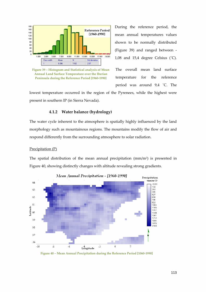
113

During the reference period, the

mean annual temperatures values

shown to be normally distributed

(Figure 39) and ranged between -

1,08 and 15,4 degree Celsius (˚C).

The overall mean land surface

temperature for the reference

period was around 9,4 ˚C. The

lowest temperature occurred in the region of the Pyrenees, while the highest were

present in southern IP (in Sierra Nevada).

4.1.2 Water balance (hydrology)

The water cycle inherent to the atmosphere is spatially highly influenced by the land

morphology such as mountainous regions. The mountains modify the flow of air and

respond differently from the surrounding atmosphere to solar radiation.

Precipitation (P)

The spatial distribution of the mean annual precipitation (mm/m2) is presented in

Figure 40, showing distinctly changes with altitude revealing strong gradients.

Figure 39 – Histogram and Statistical analysis of Mean

Annual Land Surface Temperature over the Iberian

Peninsula during the Reference Period [1960-1990]

Figure 40 – Mean Annual Precipitation during the Reference Period [1060-1990]

114

The precipitation is enhanced in some of the mountainous environments present at the

IP, having thus higher values in the west and the north of the IP as well as the Pyrenees

(over 1.000 mm/year), and lower values (<400 mm/year) at lower latitudes, i.e. obtained

toward the southeast of the IP.

There are also inland regions with a relatively low precipitation regime. The regions of

Central Mountain Range and the Estrela Saw have also presented high precipitation

values (agreeing with Daly et al. (1994) and Haiden & Postotnik (2008), which

concluded that generally, precipitation increases with elevation - although the rate

varies substantially). Moreover it is also interesting to notice the great variability of

precipitation values in close regions: the region of northern Portugal and the Galicia

region, as well as the orographic precipitation patterns in the Cantabrian region

present values widely ranging: from ~500 up to ~2.100 mm/year. However, the

relationship between precipitation and high altitudes reported in the northern regions

is different at lower latitudes, i.e., there are regions where precipitation decreases in

mountains environments. This difference of precipitation behavior relays on a

phenomenon called blocking (Houze, 2012).

FACT BOX T: The Blocking Effect description

The so-called blocking effect occurs when an air mass flowing toward mountains flows

up and over the mountain or slows down and turn to flow around them. The two

difference scenarios are dependent on height of the topography along with the moisture

content and resistance of air to rising causing different precipitation events. Generally,

warmer air is less resistant to rising as it contains a bigger moisture content than colder

air. When air flows over the mountains precipitation tends to concentrate in the wind

facing side, leading to precipitation on this side. When moist air is forced up the

windward slope it cools and expands causing water droplets to condense when the air

is saturated triggering could formation which are responsible for rain (or snow)

production over the windward side of the range (Houze, 2012).

The northern part of the IP is under conditions of consistent wind direction providing

moist air continuously and where elevations are moderate (i.e. less than 2.500 meters),

resulting in the previously discussed relationship existing between precipitation and

topography (Houze, 2012). Moreover, the Coriolis effect acting over the trade winds

115

forces the air to turn when it slows (after approaching the topography), leading to

increased precipitation on the windward side of the range - and decreased on the lee

side (Houze, 2012).

Conversely, the precipitation decreases along the range of Iberian Mountain Range and

Betic from northwest to southeast can be reflecting the decreasing of moisture supply

as winds flows over the range (Houze, 2012). On the other hand, the higher

precipitation rates located at the Northwest region of the IP are a fair example of

blocked winds by the Cantabrian Mountain Ranges (which has higher latitudes than

Iberian Mountain Range, for instance).

Conversely to what happened with the mean annual land surface temperature

variable, annual mean precipitation values are not normally distributed (Figure 41) and

instead of that the shape of the histogram suggests that this variable is lognormally

distributed. The overall mean annual precipitation estimated during the 1960-1990

period for the IP region was ~767mm/year, and values ranged between 232 and 2.107

mm/year. The lowest value occurred in the southwest region of the Peninsula, in the

region of Andalucía and in the region of Castilla y Léon located over the Central

Upland. Part of the regions of Aragon, Catalonia and Castilla-La Mancha presented as

well low values (P < 500 mm/year). These areas are another example of air moisture

loss throughout flowing air masses.

Figure 41 - Histogram and Statistical analysis of Mean Annual

Precipitation over the Iberian Peninsula during the Reference

Period [1960-1990]

116

Soil moisture (SWC)

The mean annual water content in the soil (SWC), or in other words soil moisture, was

firstly analyzed at five vertical (layers), with the thicknesses and soil depths (of mid of

the layer) disclosed in the following table:

Table 36 – Thicknesses and mid layer depth of the 5 layers of soil

Layer 1 Layer 2 Layer 3 Layer 4 Layer 5

Thickness (m) 0,065 0,254 0,913 2,902 5,700

Mid depth (m) 0,033 0,192 0,775 2,683 6,984

It should be taken into account that, despite the soil layers in the model are always the

same, if one layer is only 2 m deep, the following depths (deeper than 2 m) are not

simulated. Therefore, the thicknesses of the soil vary, and the model uses this

information for calculations. During the [1960-1990] period, the range of this variable

has gotten notoriously wider as depth increases, and the pixel distribution changes

considerably between each layer (Figure 42).

Figure 42 –

Histogram

of soil

moisture

content of

layer I [m]

of layers

1,2,3,4 and

5 during

[1960-1990]

117

One of the most glaring differences consists of the absence of pixels with value “0” for

the first two layers, contrarily to the considerable high amount existing in the layer 5,

for instance. This translates a considerable decrease of water content as depth

increases. The mean value tend to increase with depth, although the last layer (the

fifth) had a lower value than the previous one.

Figure 43 presents the spatial pattern of the mean annual soil moisture over the IP,

consisting in the combination of the soil water content from the five different layers,

resulting thus in a general layer with 9, 8 meters depth. Conversely to precipitation, the

pattern of soil moisture does not seems to be related with the altitude. In fact, despites

its lack of smooth change between SWC values, the pattern strongly resembles the

shape of the several river basins present at the IP: in center of Portugal, the highest

darker colors would be placed over the Lower Tajo Basin; in the south of mainland

Spain and spread towards the northeast direction, the shape of this wetter soil

resembles the shape of the Guadalquivir basin, while the upper shapes further up

Figure 43-Mean Annual Soil Moisture Content

during the Reference Period [1060-1990] and

comparison with the Iberian River Basins (Source: )

118

resemble the Tajo basin and upper north the Douro Basin. Close to the Pyrenees but

not has demarked as the latter shapes, it would be the influence of the Ebro basin.

It is quite noticeable the very low SWC coming inwards from the northern shore,

which is located over a region with high SWC (roughly were Asturias would sit). In

fact, the lowest SWC values went lower than 0,015 m over that place, similarly to what

occurred nearby the locations with the highest SWC in Portugal mainland. The higher

SWC values occurred in Spain, namely over Asturias and Cantabria regions, where

SWC reached up to 2,92m. The overall average annual soil water content in the IP

during the Reference Period was estimated to be ~1,1m. The values from mean annual

SWC variable, were not normally distributed, as shown in Figure 44.

Evapotranspiration (ET)

It is a common practice to set negative signal for all vertical upward fluxes as it is the

meteorological convention ( Bromwich, 2000), however, in order to enable a clear

interpretation of results, the positive signal was assigned to upward fluxes in the map

showing the mean annual evapotranspiration (ET)(mm/m2)(Figure 45). Hence, having

this present, the lowest evaporation values can be found spread in several regions:

roughly along the east Portuguese border (as well as in the south of this country) and

in southeast region of Spain and in its central region as well. The higher values can be

found in the northern regions of both countries.

Figure 44 - Histogram and Statistical analysis of Mean Annual Water

Soil Content over the Iberian Peninsula during the Reference Period

[1960-1990]

119

As a first approach, the spatial distribution of ET is moderately different from the

rainfall (i.e. precipitation distribution), but it is also correlated with altitude. The mean

annual ET distribution pattern slightly recall the spatial pattern of temperature (Figure

38), plus it also demonstrated a high correlation with the land cover type (Figure 26)

Moreover, the location and shape of lower ET values, match the same existing in the

SWC map (Figure 43).

Evaporation is also affected by the morphology since, the air consequently flows down

the lee side, contracting and warming leading to the evaporation of the water droplets,

suppressing thus precipitation (Houze, 2012).

ET changes from greater than 200 mm/year at the foot of the mountainous systems to

about 700 mm/year at the highest locations, (whereas the precipitation changed from

less than 200 mm/year at the foot of the mountain to more than 1.000 mm/year at the

tops of the mountain. An important factor affecting this variable is the type and

location of vegetation (described in Figure 26), since partly of this variable is composed

by mainly transpiration (sourced by plants). For that reason this map should be

addressed carefully since it comprises the transpiration rate as well, which is

dependent on biologic factors (such as vegetation cover transpiration processes).

Figure 45 – Mean Annual Evapotranspiration during the Reference Period [1060-1990]

120

Hence, the regions with coniferous

evergreen trees and temperate

broadleaf deciduous trees had the

highest values, (with ET > 600

mm/year) whereas the ET in crop

regions was relatively low (i.e.

ET≈150 mm/year). Finally, the

Iberian Peninsula presented a less

wide (in comparison to precipitation) range of values of mean annual

evapotranspiration (between 160 and 761 mm/year) during the annual mean for the

period from 1960 to 1990. The overall mean annual evapotranspiration was 474

mm/year (Figure 46).

4.1.3 Radiation balance

Photosynthetically Active Radiation (PAR)

The physical variable photosynthetically active radiation (PAR) over the IP is shown in

Figure 48.

Figure 47 - Mean Annual Photosynthetically Active Radiation map during the Reference Scenario

Figure 46 - Histogram and Statistical analysis of Mean

Annual Evapotranspiration over the Iberian Peninsula

during the Reference Period [1960-1990]

121

This variable can be measured either in radiometric units (W/m2) - to determine its total

energy value, or it can be measured in quantum terms, i.e. in terms of mol produced

towards photosynthesis per square meter of canopy per year (mol/m2/year) - in order

to calculate the amount of the sunlight specifically available for plant growth during a

year (Kania & Giacomelli., 2002).

Henceforth, the Figure 48 presents the spatial distribution of energy ranging between

the 400 and 700 nm along the Iberian Peninsula, for the period of 1960-1990, in

quantum terms.

The ranges of PAR values are uniformly and smoothly distributed along the latitudes,

by increasing as latitudes increases and roughly maintaining constant along the

longitudes. The lowest PAR value estimated was approximately 8.901

mol(photosynthesis)/m2(canopy)/year while the highest value was ~12.852

mol(photosynthesis)/m2(canopy)/year.

Absorbed Photosynthetically Active Radiation (APAR)

The pattern of the photosynthetically active radiation APAR (Figure 48) greatly differs

from later image presented (PAR), since it is dependent on the existence of vegetation,

as well as many other inherent factors to it (e.g. such as LAI or other features which

characterizes each type of PFT, for instance). As it can be seen from the Figure 48, the

pattern shows defined regions with higher or lower APAR values, in opposition to the

smoothness characterizing the spatial pattern of the PAR values. As a matter of fact the

pattern shown in this map strongly resembles the patterns existing in the ET map (as

well in GPP map, which will be shown afterwards).

The north and center of Portugal shown to have high rates o absorbed PAR, since

throughout roughly the entire area, APAR was above 5.205(mol

(photosynthesis)/m2(canopy)/year). In what concerns the largest areas of lower APAR

values, these regions match the same regions pointed out in Figure 41, as regions with

some of the lowest precipitation rate values.

122

Figure 48 - - Mean Annual Absorbed Photosynthetically Active Radiation during the Reference Period

The values estimated by the model, do not show a normal distribution. The lowest

value obtained for the period 1960-1990 was ~1.434 mol (photosynthesis/m2/year) and

the highest value was ~7.974 (mol (photosynthesis)/m2(canopy)/year). The overall mean

absorbed photosynthetically active radiation throughout the entire Peninsula during

the reference period was around 3.979 mol (photosynthesis)/m2(canopy)/year)(Figure

49).

Figure 49 - Histogram and Statistical analysis of Mean Annual APAR over the Iberian

Peninsula during the Reference Period [1960-1990]

123

In some areas – (such as the reddish over the Northern region of Portugal) the rate of

absorbed by canopy goes up to 60% of the maximum of PAR incident, while in other

areas – such as the blue ones in Spain presents values under the 20% of absorption of

total PAR over the place (Figure 50).

Figure 50 - Ratio APAR/PAR during the Reference Period

4.1.4 Climate variables interactions

In this section, the spatial correlation between each pair of climatic variables, over the

Iberian Peninsula during the 1960-1990 period is analyzed. Therefore, Table 37 presents

the Pearson’s Correlation Coefficients (R) between each possible combination of the

previously analyzed variables (where stronger correlations are highlighted in bold). It

should be taken into account that this correlation coefficient consists in a simplified

manner of measuring the strength of the association between two quantitative and

continuous variables – as is the case.

124

Table 37 - Coefficient correlation between climate variables estimated by JSBACH model for the

Reference period

Temperature

(T)

PAR APAR Precipitation

(P)

Evapotranspiration

(ET)

T

PAR 0,63

APAR - 0,10 - 0,11

P - 0,40 - 0,53 0,55

ET - 0,22 - 0,28 0,54 0,49

SWC - 0,12 - 0,13 - 0,12 0,06 0,3

Temperature and other variables correlation

The mean annual land surface temperature extracted across the Iberian Peninsula

during the 1960-1990 period showed a positive (+) and significant (R = 0,63) interaction

with the mean annual PAR. Roughly speaking, there was an increase of temperature

by 5 degrees driven by each increase of 1.000 mol (photosynthesis)/m2/year of PAR, as

it can be seen from the figure (Figure 51).This positive relationship was expected since

increased income of solar radiation boosts an increase of land surface temperature as a

result of radiation absorption. Furthermore, it is easily perceived from the comparison

between both PAR and T map (Figure 48 and Figure 39), that mean values tend to

increase at southern latitudes. The results of the correlation between land surface

temperature and the rest of the variables i.e., APAR, precipitation, evapotranspiration

and soil moisture presented a negative (-) and les strong relationship.

Another moderate (but less strong) correlation is the interaction between temperature-

precipitation, which is shown in Figure 51. The result of this negative relationship also

makes sense since these two variables are closely related due to being strongly

dependent on each other. Comparing the temperature and precipitation maps (Figure

38 and Figure 40), the highest precipitation occurred roughly in the regions with lower

mean annual land surface temperature such as at higher latitudes, and vice-versa for

southern regions. The strength of this relationship (i.e., the fact of being moderate

R=0,40) results from the fact that there are multiple places where higher temperatures

do not imply lower precipitations

125

Nevertheless, temperature and precipitation spatial patterns should be interpreted

considering the strong co variability that exists (Kevin et al., 2005). In order to rain the

temperature needs to rise so that water evaporates generating clouds formation

(Buishand & Brandsa, 1999). However, as it can be seen in the south Portugal and the

region of Andalusia, higher temperature did not lead to higher precipitation. The

explanation for this fact could rely on the fact that higher temperatures lead to higher

saturate vapor levels causing a higher capacity of the warm air to contain higher

moisture amount than cold air

The negative (even though small) relationship existing between temperature and

evapotranspiration, is a reasonable result, since higher rates of evapotranspiration

promote cloud formation causing less radiation penetration into the atmosphere

resulting in lower land surface temperatures. Similarly to others, this interaction is no

linear since there are many other factors affecting both variables such as the

precipitation and heat latent flux, for instance.

PAR, APAR and other variables correlation

The second stronger relationship occurred between PAR and precipitation (R=-0,53),

being negatively correlatd. As it can be interpreted from the comparison of Figure 41

and 48, higher rates of income PAR over certain areas, driven lower precipitation rates

there.

The PAR and APAR relationship is positive (+)– since the latter consist in the amount

from PAR which was actually absorbed by the plant, hence higher incomes of PAR will

enhance photosynthetic processes resulting in greater amounts of radiation being

absorbed during that process. These two variables are moderately correlated (R=0,55),

since the spatial distribution of APAR is constrained mostly by vegetation cover – thus,

APAR spatial distribution do not follow the same patter as PAR.

The positive (+) relationship existing between both precipitation and

evapotranspiration and the APAR variable, is expected, since APAR denotes the

existence of vegetation. Hence, more precipitation will enhance photosynthesis,

triggering the increase of photosynthetically active radiation being absorbed by plants

126

leading to a. higher the rate of photosynthetically processes and ultimately a higher

transpiration rate by plants as a consequence of that process.

Evapotranspiration and other variables correlation

Finally, the comparison of the spatial patterns of mean annual precipitation and mean

annual evapotranspiration (Figure 40 and Figure 45) shows that areas where

precipitation rate is higher evapotranspiration rate tend to be higher: the higher the

water supply throughout rainfall processes, the bigger the amount of water possible to

be evapotranspirated resulting in a positive and moderate relationship (R=0,49). As it

can be seen from the Figure 51, this interaction is stronger when precipitation rate

ranges between ~250 and ~800 mm/m2/year.

127

Figure 51 - Correlation between climate variables during the Reference Period

128

4.2 Carbon balance analysis – Reference Period

The analysis of the carbon balance during the reference period aims to assess the

spatial distribution of carbon uptake and productivity of vegetation across the Iberian

Peninsula. The variables taken into account are the gross primary production, the net

primary production and biomass spatial distribution during the 1960-1990 period. Both

productivity and biomass are segregated by herbaceous and forest biomass types. This

set of results will serve as reference to the assessment of change in vegetation response

to the climate changes projected in future scenarios. The spatial correlation of carbon

variables and climate variables are also assessed for the reference period.

4.2.1 Gross Primary Production (GPP)

Corroborating Polley et al. (2011), the gross primary productivity (GPP) map consists in

a key component of the carbon (C) cycle, enabling the understanding of spatial

patterns in C fluxes. Consequently, the map shown below (Figure 52), depicts the areas

with higher carbon production (and therefore higher carbon uptakes). The highest

rates of GPP are located in the north of Portugal (more specifically the region above the

Tejo river); in Galicia, along the north shore of Spain (including the Pyrenees) and

along the Central Mountain System. This pattern resembles thus the temperate zone,

Figure 52 – Mean Annual Gross Primary Production (GPP) during the Reference Period [1960-1990]

129

which matches the areas of higher precipitation and APAR rates. The mean annual

GPP during the Reference period ranged between ~1.141 and ~9.373 g(CO2)/m2, having

an overall mean of ~4.422 g(CO2)/m2.

Environmental Controls on GPP

In order to assess how is GPP controlled by the previously regarded climate factors, the

spatial correlations between GPP and temperature, precipitation, evapotranspiration,

soil moisture, PAR and APAR were evaluated by calculating the correlation

coefficients (R) over the Iberian Peninsula (Table 38), enabling hence to take

conclusions regarding the strength of relationship of their spatial patterns.

Table 38- Correlation coefficients for GPP and climate variables during the Reference Period [1960-

1990]

Temperature Water Balance Radiation

P ET SWC PAR APAR

GPP -0.25 0.65 0.76 0.12 -0.36 0.81

Among all the factors, precipitation, evapotranspiration and APAR were more strongly

correlated with GPP during the 1060-1990 period. On the other hand, the impact of

land surface temperature (T) and PAR had a weak and negative (-) correlation with the

GPP, meaning that these environmental variables were the least significant among all.

The negative relationship means that, spatially, the GPP increased in regions where

temperature and PAR mean values lowered.

In what concerns soil moisture or soil water content (SWC), the resulting relationship

was considerably lower than expected (since soil water content plays such an

important role on productivity). The relationship is positive (+) and one of the most

probable reasons for the evident low relationship, is the fact that this variable is not

regarding merely the amount of water which is actually available to the roots.

Moreover, the relationship between GPP and soil water content vary: trees are able to

store water and nutrients and to tap water from deeper soil horizons (Davis et al., 1998;

Oliveira et al., 2005). For the same reason earlier explained, precipitation is not equal to

water available to vegetation (Liu et al., 2011) and hence that would explain the less

strong correlation between the pair GPP vs precipitation than the pairs GPP vs ET and

130

GPP vs APAR - even though water is known to be a limiting factor in this environment

and that it plays a great impact on the interannual variability. Notwithstanding this

variable was shown to be linearly correlated with GPP (Figure 53) and its coefficient of

determination R2 shows in fact that this linear regression fits moderately to the

relationship between GPP and P.

Figure 53 - Relationship between GPP and Precipitation and GPP and Evapotranspiration during the

Reference Period [1960-1990]

The strong relationship between GPP

and ET is explained by the fact that

plant transpiration and photosynthesis

are strongly coupled as well as due the

fact that stomata are the pathway for

absorbing CO2 and releasing water

vapor by transpiration. Hence this

strong and positive correlation is in

accordance with the expected (i.e. high GPP corresponding with high ET, and vice

versa (Lu & Zhuanf, 2010; Running & Zhao, 2005). The correlation between these two

variables will hence be used as another source of information to depict the water use

efficiency, i.e. the ratio of GPP to ET, in a forthcoming chapter. Looking closely to the

pattern of ET and P maps (Figure 40 and Figure 45) and comparing them with the GPP

map (Figure 52), in fact the ET pattern is noticeable far more resembling (namely the

existing areas of considerable lower values from both variables)(Figure 54).

Moreover, as it can be also seen, the southeastern quadrant of the P map, lacks some

patterns that are present in ET and P maps. Similarly to the precipitation variable, the

Figure 54 - Comparison of spatial distribution between

GPP, P and ET during [1960-1990]

131

evapotranspiration also present a linear correlation with GPP (Figure 53), although it is

less well explained by the linear functions (since the coefficient of determination is

smaller, i.e. R2 = 0,42). The coefficients correlations between annual GPP, precipitation

and temperature are in accordance with Jung et al. (2011) (since these correlations are

positive and higher than 0,4.

The strongest relationship (i.e. correlation between GPP and APAR) is expected, since

GPP describes the total light energy that has been converted to plant biomass

(Anderson et al., 2009). Furthermore, GPP and APAR can be combined as

(Equation 8)

(where ε stands for conversion efficiency which is dependent upon vegetation type

(Anderson et al., 2009.)). Since GPP is proportional to the APAR (Monteith, 1972; Xiao

et al., 2005) these two variables showed - not surprisingly – to be strongly and

positively correlated (R=0,81) (Figure 55) and present the greatest R2 among all

variables relationship. The evident strong relationship among these two variables has

also driven the interest on studying forwardly, the so-called light-use efficiency (LUE),

which is derived from empirical observations of GPP and APAR (Monteith, 1972).

Figure 55 –The relationship between GPP and APAR at the IP during the 1960-1990 period.

132

Water-Use Efficiency (WUE) during the Reference Period

The water-use efficiency across the IP, during the [1960-1990] period is found in Figure

56 and it is expressed in terms of grams of CO2 uptake for each mm of water from

evapotranspiration flux. By visual interpretation of Figure 26, the plant functional type

is an important factor to determine the spatial pattern. For the northern region of

Portugal (which is a C3 grass dominated system – followed by coniferous evergreen

trees) the WUE showed higher values – greater than 11 g(CO2)/mm(H2O). The region

located in the south and southwestern part of the IP (bordered by the Baetic Mountain

Range and the Central Mountain System), showed evenly WUE values ranging

between 8 and 9 g(CO2)/mm(H2O) consisting thus in a significant difference between

this C4 grass and C3 crop dominated site and the site firstly addressed. These WUE

differences are because of PFT-oriented parameterizations .

The right half of the IP presented mainly lower WUE values (consisting mainly in a C3

crop dominated site), but there are also areas of great WUE (greater than 14

g(CO2)/mm(H2O). The overall mean value of WUE over the area of study was around

9,2 g(CO2)/mm(H2O).

Figure 56 - Mean Annual WUE during reference period

133

Hence, these results mean that even though that mean annual precipitation and ET are

similar over these areas, the higher WUE existing over some region, enable them to

uptake more carbon during the growing seasons than regions with lower WUE values.

Another important result that can be taken from here is that once again the ecosystem

difference in atmospheric CO2 concentration as well as CO2 and water fluxes, have

important management implications including primary productivity, C sequestration

and rangeland health.

Light-Use Efficiency (LUE)during the Reference Period

There were significant differences in LUE occurred during the 1960-1990 period over

the territory due to differences in soil water content (as it resembles this map, when it

comes to pattern distribution) (Figure 43). It also corroborates the findings of Polley et

al. (2011), who have depicted the existence of a great relationship among these LUE

and soil water content.

Figure 57 - Mean Annual LUE during the Reference Period

134

For the reference period, the values of LUE varied between 0.34 and 1.62

g(CO2)/mol(photosynthesis) and the overall mean LUE was ~1.16

g(CO2)/mol(photosynthesis)(Figure 57).

4.2.2 Net Primary Production (NPP)

The results regarding the Net Primary Production (NPP) are segregated by forest and

herbaceous biomass (Figure 59 and Figure 60) – and NPP is expressed similarly to GPP.

The spatial patterns of both biomass types are considerably different. The NPP from

forest biomass varies more abruptly and the higher values are located along the

Temperate zone of the IP. The herbaceous biomass has shown to be more evenly

distributed across the territory, showing less evidently the pattern of bioclimatic zones,

although it discriminates better locations with lower annual SWC and

evapotranspiration regions (which could mean that grasses are more responsive to

water scarcity than forest biomass).

The highest mean annual NPP for forest biomass were found in the northwest part of

the Iberian Peninsula (accounting with ~2.699 g(CO2)/m2(grid box) whereas in some

areas namely over the Southern Plateau showed no existence of NPP. The overall mean

annual NPP over the IP during the reference period was approximately 450

g(CO2)/m2(grid box).

Figure 58- Mean Annual Forest Net Primary Production (NPP) during the Reference Period [1960-1990]

135

The mean annual NPP underlying the herbaceous biomass during the same period,

reached higher values (up to 2.890 g(CO2)/m2(grid box) and having an overall mean of

~1.531 g(CO2)/m2(grid box).

Figure 59 - Mean Annual Herbaceous Net Primary Production (NPP) during the Reference Period [1960-

1990]

The spatial distribution of NPP did not show the same pattern as ET across this large

elevation range.. These different spatial patterns might be due several processes, such

as the autotrophic respiration and the intersectional water loss and evaporation from

soil (Sun et al., 2004).

NPP and GPP correlation

The mean annual NPP of all biomass present at the IP (i.e. both herbaceous and forest

biomass) was, as expected, strongly and positively correlated with the mean annual

GPP, having a great coefficient correlation, R = 0,88. From the picture below (Figure

60), (along with the coefficient of determination R2) denotes that the linear association

between NPP and GPP is very strong since (R2 = 78%).

136

Figure 60 - Regression analysis between mean annual GPP and NPP (from all biomass) over the Iberian

Peninsula during the Reference Period

4.2.3 Biomass

The followings figures, present the biomass estimations over the IP, segregated in

“Forest” biomass (Figure 61) and “Herbaceous” biomass (Figure 62). These maps do

not present biomass in absolute terms, but in “areal density” of biomass, since it

expresses the amount of mass of carbon per unit area.

Figure 61 - Mean Annual Forest Biomass Density during Reference Period [1960-1990]

137

Figure 62 - Mean Annual Herbaceous Biomass Density during Reference Period [1960-1990]

The regions with higher densities of forest biomass (i.e. amounting above 5.500

g(C)/m2) are located in the northern IP; in the northern regions of Portugal and at the

highest altitudes from the Central Mountain Range, matching the Temperate

bioclimatic zone (Figure 17), where mean annual precipitation values were above 1.000

mm/year. The Mediterranean regions present hence lower densities of forest biomass

density. The locations with lower density values are shown to be over the Central

Plateau and also over the river basins of Tejo, Douro, Ebro and Guadalquivir rivers

(see Figure 43 for comparison), with values below 600 g(C)/m2. Although some

variables have a similar pattern (such as mean annual APAR), the mean annual

precipitation spatial pattern (Figure 40) has the most similar pattern to forest biomass

areal density.

Multiple cells (537), corresponding nearly to 50% of the Iberian territory, have shown

values densities of forest biomass to be zero g(C)/m2) – which denotes an absence of

forest biomass. The maximum value of annual mean forest biomass during the

reference period was ~9.744 g(C)/m2 and the overall mean was ~1.503 g(C)/m2 (Figure

63).

138

Figure 63 - Statistical analysis of Mean Annual Forest Biomass during [1960-1990]

The spatial pattern of herbaceous aerial densities did not show to be correlated with

bioclimatic zones as forest biomass did. Both northern part and southeastern quadrant

of the IP shown to have low values of herbaceous biomass density, and the lowest

values were located in the territory of Portugal. The location of low densities of

herbaceous biomass strongly resembles the map of the spatial pattern of mean annual

soil moisture and evapotranspiration (Figure 43 and Figure 45), which could indicate

that these type of biomass is strongly affected by water scarcity. The highest values

accounted with ~353g (C)/m2 while the lowest densities of herbaceous biomass were

~10 g (C)/m2. The overall mean annual herbaceous biomass density during the

reference period was ~190 g(C)/m2 (Figure 64).

Figure 64 - Statistical analysis of Mean Annual Herbaceous Biomass during [1960-1990]

139

In terms of absolute biomass, i.e. total amount of biomass estimated for the 1960-1990

period in terms of mass, as fairly expected, the “Forest” biomass presented a much

larger contribute (up to 78%) than “Herbaceous” biomass, which accounted with 22%

of the total biomass estimated over the Iberian Peninsula during the Reference period.

Figure 65 shows a chart pie summarizing the overall results from “Forest” biomass and

“Herbaceous” biomass. Despite the large land areas with agriculture, the higher

enrichment in fibber of trees results in a much greater mass.

Figure 65 - Percentage and absolute values of Forest and Herbaceous Biomass during the Reference

Period [1960-1990]

The mass of biomass discriminated for each PFT presented in IP is shown in Figure 66.

The greater biomass contributing to the overall scheme, are from Coniferous evergreen

tress (which accounted in 1960-1990 period with ~4,24 x108 tonnes) and broadleaf

deciduous trees (accounting with 3,02 x108 tonnes). In fact, together these two PFT

accounted with 95% of the overall “Forest” biomass type. Within the same biomass

type, both temperate broadleaf evergreen trees and rain green shrubs accounted each

one of them with 2% of the overall biomass from forests. In last place comes the

deciduous shrubs, which contribute was almost negligible.

140

Figure 66 - Estimations of Biomass assigned to each PFT, during the Reference Period [1960-1990]

In what concerns the “Herbaceous” biomass, the contribution of each PFT to the

overall amount of biomass was more even: 45, 26, 20 and 9% for C3 crops, C3 grasses,

C4 grasses and C4 crops, respectively.

Environmental Controls on Forest and Herbaceous Biomass

Similarly to the section assessing the environmental controls on GPP, this section

assesses how climate variables are correlated (in spatial patterns) to both sets of

biomass (herbaceous and forest biomass) through the correlation coefficient R (as well

as the graphic visualization of each variable against the other). These comparisons

enable to understand the strength of the relationships between the two sets of biomass

and climate variables existing back in 1960-1990 period – and their differences. Table 39

shows the summary of the coefficient correlation each climate variable-biomass type

pair (the strongest correlations are highlighted in bold).

141

Table 39 - Correlation coefficients between Biomass and Climate Variables during the Reference Period

Water Balance Radiation

T P ET SWC PAR APAR FOREST BIOMASS -0,436 0,692 -0,457 0,184 -0,536 0,702

HERBACEOUS BIOMASS 0,175 0,097 -0,059 -0,049 -0,024 0,028

Forest biomass shown to be moderately and negatively correlated with land surface

temperature distribution (Table 39) which is explained by the fact that the locations

with higher amounts of forest biomass which are located in the temperate zone –

where mean annual temperatures are lower (Figure 38). These areas of lower

temperatures (i.e. T<9˚C) are wider and more disperse than the locations with high

densities of forest biomass. Herbaceous biomass shown to have a weak (and positive)

relationship with land surface temperature.

The comparison of the correlation coefficients between precipitation-forest biomass

and precipitation-herbaceous biomass (Table 39), confirms the assumption earlier

made in 4.2.3, i.e. forest biomass is likely to be more strongly spatially affected by

precipitation than herbaceous biomass. Forest biomass shows hence a negative and

moderate correlation with mean annual evapotranspiration (while herbaceous biomass

relationship was negligible).

Hence, summarizing and rating all the significant correlations (i.e. which upward the

value of 0,4), it comes that forest biomass mostly depends on APAR, followed closely

by precipitation and then PAR, temperature and finally evapotranspiration, having a

negative relationship with the three later. On the other hand, herbaceous biomass

showed to be no meaningfully correlated with the climate variables (Table 39).

Figures 68, 69, 70, 71 and 72 provide a graphical analyzes of the correlation between

the climate and environmental variables and the biomass variables. Henceforth, The

correlation of mean annual land surface temperature and the amount of biomass

modeled for the reference period, showed that both biomass types are likely to be able

to harvest carbon, (i.e. to generate biomass) under a optimal range of annual land

surface temperature between 10 and 15˚C degrees – (the extremes of this range in fact

nearly match the total and maximum mean temperature verified during 1960-1990).

142

However for the herbaceous biomass, the amount of biomass does not seem to vary

considerable during this range of temperatures. On the other hand, the forest biomass

seems to have higher rates of biomass generation between ~6 and 9 ˚C degrees, and

after the 14˚C biomass rates tend to decrease (Figure 67). For the biomass-precipitation

interaction, it is noticeable a difference of the response between the herbaceous and

forest biomass to the mean annual precipitation during the reference period. The

interaction of the herbaceous biomass resembles a logarithmic behavior – the biomass

increase rapidly until the ~600 mm/year and after this, the maximum values tend to

stabilize (Figure 69). Forest biomass increases less rapidly for small mean annual

precipitation values, (i.e. until ~500 mm/year) after which it starts to increase reaching

the maximum values between the ~1.000 and ~4.000 mm/year of precipitation (Figure

69).

In what concerns the response of biomass to the mean annual evapotranspiration, the

herbaceous biomass behaves smoothly having a biomass rate ranging between ~9 and

~28 mol(C)/m2 within the approximate rage of evapotranspiration 700 and -500

mm/year, after which tends to decrease (Figure 70). Conversely, the forest biomass

showed a general decrease tendency of biomass values as evaporation rates decrease.

Furthermore, for values higher than 600 mm/year, the biomass values are greater than

100 mol(C)/m2, however, after this evaporation values, the range of biomass becomes

wider (reaching the lowest values estimated for biomass). The maximum values of

biomass for forest biomass were estimated to occur for evaporation rates ranging

between 600 and 500 mm/m2 (Figure 70).

Finally, for soil water content, both herbaceous and forest biomass, showed to be

poorly related to this variable, since it the values ranged around the same values.

Forest biomass showed though three peaks of lower biomass values for the ranges

~0,25-0,500, ~1,00-1,30 and 1,60-1,75 m of soil water content (for the first soil layer).

Finally, the response of herbaceous to mean annual PAR seems was barely noticeable,

conversely to forest biomass which seems to have slight increase of biomass

production for lower values of PAR (i.e., the highest biomass values were found to

occur within the range of ~8.900 and 11.000 mol(C)/m2 of PAR). For APAR variable

143

(and similarly to what occurred with the response to the annual precipitation rate

variable), the herbaceous biomass response to APAR resemble a logarithmic behavior

while the forest transpired an tendency of increasing biomass values with increasing

APAR rates resembling a exponential behavior. Forest biomass shows increasingly

higher values after the ~4.000 mol (photosynthesis)/m2. After the ~6500 mol

(photosynthesis)/m2 biomass values are higher than 200 mol(C)/m2 (Figure 72).

Figure 67 - Correlation between mean annual temperature and herbaceous/forest biomass during the


Figure 68 - Correlation between mean annual precipitation and herbaceous/forest biomass during the


144

Figure 69 - Correlation between mean annual ET and herbaceous/forest biomass during the Reference

Period [1960-1990]

Figure 71 - Correlation between radiation variables and herbaceous/forest biomass during the Reference

Period [1960-1990]

Figure 70 - Correlation between mean annual SWC and herbaceous/forest biomass during the Reference

Period [1960-1990]

145

4.3 Climate Variables Change Analysis – Futures Scenarios

The climate variable change analysis performed in this section assesses the changes

occurred for each climate (and environmental) variable earlier addressed, projected for

the future time periods, in comparison with the reference period. Hence, (similarly as

in the climate variables analysis for the reference period), the spatial pattern of each

projected climate variable is analyzed along with its magnitude of change. In some

cases (whenever meaningful) its absolute difference from reference period is also

analyzed. These analyzes enable to assess the locations subject of greater changes

which will ultimately enable the understanding of how these changes in climate will

likely affect future vegetation productivity and biomass (which will be addressed in

the carbon balance analysis for future scenarios).

It should be noticed though that the variables that are model data inputs refer to two

future scenarios, namely 2060-2090 and 2070-2100. However, the climate variables that

are model data outputs (e.g. soil moisture, evapotranspiration, APAR, productivity

and biomass variables) are regarded in four future scenarios, namely 2060-2090 and

2070-2100 whit CO2 levels assumed to be constant (C1 and C2 scenarios, respectively),

and future scenarios 2060-2090 and 2070-2100 with CO2 levels considered to rise (E1

and E2 scenarios, respectively). After each climate variable change analysis, a

comparison of other studies (which regarded climate variables for the same IPCC

scenario, i.e. A1B scenario) was made at an Iberian and global scale, allowing

understanding how different or accurate JSBACH results are in comparison with

literature results.

4.3.1 Land surface temperature (T)

The mean annual land surface temperature variable is projected to maintain the same

general geographic pattern existing in the 1960-1990 period, as it can be compared with

Figure 38, for both future time aggregations scenarios 2060-2090 and 2070-2100 (which

will be hereafter addressed as C1 and C2 scenario whenever the CO2 level is not

relevant as is the case of every variable consisting in model data input). Although, the

main difference between these two scenarios and the reference period, consists in the

fact that the mean land surface temperature values have increased throughout the

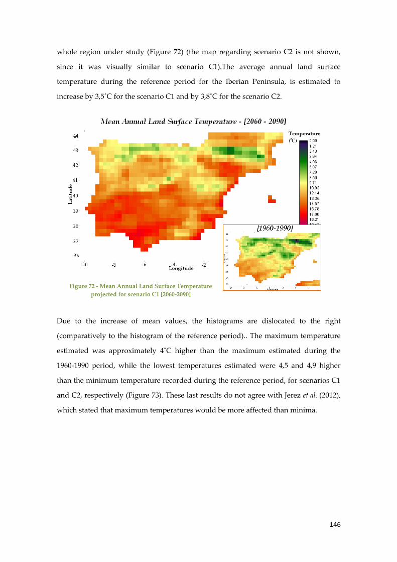
146

whole region under study (Figure 72) (the map regarding scenario C2 is not shown,

since it was visually similar to scenario C1).The average annual land surface

temperature during the reference period for the Iberian Peninsula, is estimated to

increase by 3,5˚C for the scenario C1 and by 3,8˚C for the scenario C2.

Due to the increase of mean values, the histograms are dislocated to the right

(comparatively to the histogram of the reference period).. The maximum temperature

estimated was approximately 4˚C higher than the maximum estimated during the

1960-1990 period, while the lowest temperatures estimated were 4,5 and 4,9 higher

than the minimum temperature recorded during the reference period, for scenarios C1

and C2, respectively (Figure 73). These last results do not agree with Jerez et al. (2012),

which stated that maximum temperatures would be more affected than minima.

Figure 72 - Mean Annual Land Surface Temperature

projected for scenario C1 [2060-2090]

147

As shown in Figure 74, under the scenario C1, the overall increase of annual mean land

surface temperature over the IP,is higher than the global temperatures predicted

within the A1B scenario for global surface warming (which ranges between 2,3 and

2,8⁰C) (IPCC, 2007). Furthermore, Figure 74 enables as well to understand that the

highest changes in temperature are expected to occur in the center and Northeast

region of the Iberian Peninsula, while the smaller changes are associated to regions

closer to the shore.

Figure 74 – Multi-Model Averages and Assessed Ranges for Surface Warming (Source: Adapted from

IPCC, 2007)

The Pyrenees and the highest points of the Iberian Peninsula exhibit considerable

strong mean annual land surface temperature changes. Some pixels of the image

showed a percentage change upper than 100% in Scenario C1, when comparing to the

reference period. The image below (Figure 75) shows the difference in percentages

Figure 73 – Histograms and Statistical analysis of Land Surface Temperature for Scenarios C1 and C2

148

between future scenarios against the reference period. Moreover, the results show that

in fact, the temperature rise occurs in all parts of the region under study.

Both

maps regarding the percentage changes of differences between the future period

scenarios [2060-2090] and [2070-2100] and the reference period ranges from 16 up to

nearly 300%. The strongest changes occurred mainly over the mountain ranges existing

in mainland Spain (being spatially wider in Iberian Mountain Range) as well as in the

Pyrenees. Warming temperatures are thus, likely to become more pronounced in the

mid continental areas at higher altitudes; whereas the lower rises are located in the

North and South Portuguese shore (ranging roughly between 17 and 25%).

Figure 76 presents the pattern of change between both future scenarios, showing that

the areas with greater percentage changes are wider over the mountain ranges. The

maximum change occurring between 2060-2090 and 2070-2100 periods is around 11 %.

Figure 75 - Percentage Change of Mean Annual Land Surface Temperature between Reference

Period [1960-1990] and Scenario C1 [2060-2090]

149

The overall mean of percentage change of land surface temperature for the scenario C1

in comparison to the reference period was estimated to be around 38% (and 41% for

scenario C2-Reference period comparison). In coastal areas the percentage change has a

percentage changes ranging between 17 and 25% approximately, while the inner land

areas have stronger changes, between 40 and 55%. Although the most accentuated

changes occurred at regions with higher altitudes such as the highest points in the

cordilleras (with temperature changes going further than 170% percentage change of

temperature), and basically along the Pyrenees. In fact there were verified the highest

temperature changes of the Iberian Peninsula (some grid cells presented values around

200%). The percentage change of land surface between the scenario 2 and 1 has also

verified positive changes although considerably lower than the first comparison, with

values ranging between ~1% and 11%. The mean change between the two futures

scenarios was ~3% and the pattern of percentage change was similar to the previously

addressed.

Figure 76 - Percentage Change of Mean Annual Land Surface Temperature between Scenario C1

[2060-2090] and Scenario C2 [2070-2100]

150

4.3.2 Water balance

Precipitation (P)

Similarly to the previous variable, the mean annual precipitation during both future C1

and C2 scenarios across the Iberian Peninsula keeps the same pattern as in reference

period (Figure 77). Despite the same pattern, annual precipitation is projected to

decrease. Overally, across the Iberian Peninsula, the mean rate was estimated to drop

by ~195 and ~206 mm by 2060-2090 and 2070-2100, respectively.

The

histogramsare dislocated to the left – since the mean precipitation rates decreases in

2060-2090 and 2070-2100 peridos (Figure 78), but still they maintain a shape resembling

a lognormal distribution.

Figure 78 - Histograms and Statistical analysis of Precipitation for Scenarios C1 and C2

Figure 77 - Annual Mean Precipitation during

Scenario C1 [2060-2090]

151

The following images (Figure 79), presents the percentage change existing between the

reference period, and each of the future scenarios. The percentages are represented as

positive values, and they translate into the amount of the precipitation rate that has

decreased from the reference period. For instance, if the value of a grid cell existing in

the reference period decreased its precipitation rate from 1.000 mm/m2/year to 200

mm/year, which would imply a decrease of precipitation rate (within that grid cell) of

80%.

The

entire southern and most of eastern quadrant of Spain, were the regions with the

biggest decreases in precipitation rate from reference period to scenarios C1 and C2. In

fact, in the latter period, the decrease in precipitation went up to 70% of the

precipitation value existing during the reference period.

Figure 79 - Percentage Change of Mean Annual Precipitation between Reference Period [1960-1990]

and Scenarios C1 (upper image) and Scenario C2 (bottom). In this case, positive change refers to

decrease in precipitation. Redish areas present higher decreases in precipitation and greenish areas

present lower decreases in precipitation.

152

The northern regions – matching with the Iberian Temperate Climate region consisted

thus in the region with the least changes – ranging between ~5 to ~30%. The low range

of change at these places may be due to the fact, that those areas had in fact the highest

precipitation rates in the Iberian Peninsula during the reference period - and thus, in

terms of absolute values, a considerable decrease will not result in terms of percentage,

in a significant change when compared to a place with lower precipitation rates (Figure

79). In what concerns the summary statistics (Figure 80), the overall change results

across the entire Peninsula are that the mean annual precipitation is expected to

decrease in roughly 37% of its value from the 1960-1990 period, while this value

decreases for up to nearly 40% by 2070-2100. Furthermore, the entire area will have a

decrease of at least 5% of the average annual precipitation existing during the reference

period.

The previous results for Iberian Peninsula are contrary to some published results. As it

can be seen from the picture below (Figure 81), at least one climate model has

predicted rises in precipitation (i.e. ΔP>0) rates for the northern part of the IP region

(orange color is assigned to one model).

Figure 80 - min c1~5,2 mm/m2/year min c24,8

153

Figure 81 – Number of models which simulate a precipitation increase between the time periods 2080-

2099 and 1980-1999 for the scenario A1B (Source: Höschel et al., n.d.)

Moreover, comparing the trends of mean annual global precipitation and mean annual

global precipitation over the IP by the next century and under a A1B scenarios

projections, the results are considerable different (Figure 82): they predicted an overall

increase in precipitation by 5 and 4,5% between the period 2060-2090 and the period

1980-1990 and between the period 2070-2100 and the period 1980-1990, respectively.

Figure 82 - Time series of globally averaged precipitation change (%) from various coupled

models for Scenario A1B and E1, relative to the 1980-199 annual average (Source: Adapted

from Höschel et al., n.d.)

154

Soil moisture (SWC)

The mean annual soil moisture modeled by JSBACH model for the scenario C1 (Figure

83) does not present great visual differences from the remaining scenarios C2, E1 and

E2. The maximum values of SWC have decreased for the scenarios “C”: from 2,74 to

2,72m – corresponding to scenarios C1 and C2; and remained roughly constant for both

scenarios E1 and E2 (i.e. SWC ≈ 2,82m). The minimum values remained roughly

constant as well, for the overall set of future scenarios (i.e. SWC≈ 0,013m).

Figure 83 - Mean Annual Soil Moisture Content during Scenario

C1 [2060-2090]

The overall mean annual SWC values, have also

decreased for all scenarios even though the scenarios “C” showed higher decreases,

namely 0,86 and 0,84 for C1 and C2, respectively – and 0,93 to 0,91 from scenario E1 to

E2 (Figure 84).

155

Figure 84 - Histograms and Statistical Analysis of Mean Annual SWC during Scenarios C1, C2, E1 and

E2

Hence, regarding now the overall average magnitude of change, there was a notable

reduction of average SWC over the IP in the Scenario C1 and C2 – i.e. -22% and 25%,

having the 1960-1990 as basis. Although not so strong, the decline of SWC also

occurred for Scenarios “E” (a reduction by 16 and 18% of decline, for scenario E1 and

E2, respectively). Comparing now the Scenarios “E” and “C”, the scenarios assuming

rising CO2 depict hence a less strong loss of soil water content than the scenarios of

constant atmospheric CO2. The difference between scenario E1 and C1, and the

scenarios E2 and C2 were respectively 8 and 9%.

The overall tendency of decreasing soil moisture was fairly expected, due to the

decrease of water input (since precipitation rates were projected to decrease was well

i.e. this variable is mainly controlled by water supply). In fact, the percentage changes

of both precipitation and SWC for 2060-2090 and 2070-2100 periods are in the same

order of magnitude (i.e. above 20% of change).

In comparison with IPCC (2007), the results modeled by JSBACH model were

substantially the same: as it can be depicted from the Figure 85, the IP region was

modeled to suffer a decline by 20% (reddish colors in the map),

156

Figure 85 - Multi-model (10 models) mean change in soil moisture content (%). Changes are annual

means for the SRES A1B scenario for the period 2080 to 2099 relative to 1980 to 1999. The stippled

marks the locations where at least 80% of models agree on the sign of the mean change (Source: IPCC,

2007)

Evapotranspiration (ET)

In the mean annual evapotranspiration forecasted for scenarios C1, C2, E1 and E2

scenarios, the Spanish territory verifies the most accentuated changes, mainly in the

regions of Castilla y Léon, Aragon, Castilla-La Mancha, Estremadura and Andalucía

(as it can be seen in the Figure 86 the color became “brighter”, meaning a decrease

evapotranspiration over the region)

Figure 86 - Mean Annual Evapotranspiration during

Scenario C1 [2060-2090]

157

The changes consisted mainly in the decrease of evapotranspiration in the regions

mentioned above – for the Scenario C1 the overall annual mean evapotranspiration

was projected to be ~415 mm/year, and ~407 mm/year for Scenario C2, whereas for the

E1 and E2 scenarios these values drop to ~401 and ~393mm/year (Figure 87). The

difference between the maximum and minimum value of evapotranspiration rate,

became wider during the scenario C1 (ranging approximately between ~125 and 810

mm/year) (while for the scenario C2 the values ranged between ~118 and ~809

mm/year), which means, that the minimum rate value became lower and the maximum

rate value became higher. In other words, the rates became more extreme. While for

the E1 and E2 scenarios the evapotranspiration variable ranges between [123 –

776]mm/year and [116-769]mm/year, respectively.

Figure 87 - Histograms and Statistical Analysis of Mean Annual Evapotranspiration during Scenarios

C1, C2, E1 and E2

The overall decrease trend can be due to the fact that evapotranspiration are

potentially driven by changes in mean temperature and precipitation (besides other

factors). Therefore, since as presented in earlier results, once that that precipitation is

decreasing and temperature are rising it could lead to less water supply resulting in

lower levels of evapotranspiration processes (lower levels of evapotranspiration lead to

less cloud formation, boosting the income of radiation). In terms of magnitude of

change (i.e. in percentage change), the scenarios C1 and C2 showed a decrease of 15

and 16%, respectively whereas the scenarios E1 and E2 had a higher decrease: -16 and -

158

18% of the mean annual evapotranspiration during the reference period. Comparing

this to other values, the overall trend of decreasing evapotranspiration rate across the

IP is similar to what was forecasted by Kim et al.(2002.)(Figure 88).

Figure 88 - Differences between global mean ET during the period 1960-1990 and 2070-2100. Simulation

results from ECHAM5 with IPCC climate scenario A1B (Source: Kim et al., 2002)

The greenish-blue color even though it is hard to define by the greenish-blue color over

the IP region, the value ranges match approximately the same range that the previous

map presented (i.e. decrease of evapotranspiration around ~70mm/year). However, the

changes in evapotranspiration rate have different behaviors throughout the rest of the

world, due to the different hydrological (and biological factor presents in each one of

them (Kim et al., 2002)).

A plausible reason that could explain the differences between the Scenarios “C” and

“E” (i.e., the higher decreases in the scenarios assuming elevation of atmospheric CO2

concentration compared to “C” scenarios) could be the direct effect of atmospheric CO2

enrichment. Under elevated CO2 concentrations conditions, the plants do not open

their leaf stomatal pores as wide as they do, under lower levels of atmospheric CO2

concentration. Moreover, they also tend to produce less stomata per unit area of leaf

surface at higher levels of atmospheric CO2. Both changes will hence reduce the rate of

transpiration, implying does the greater decrease forecasted to Scenarios “E” in

comparison the scenarios “C”, where CO2 rise is not taken into account.

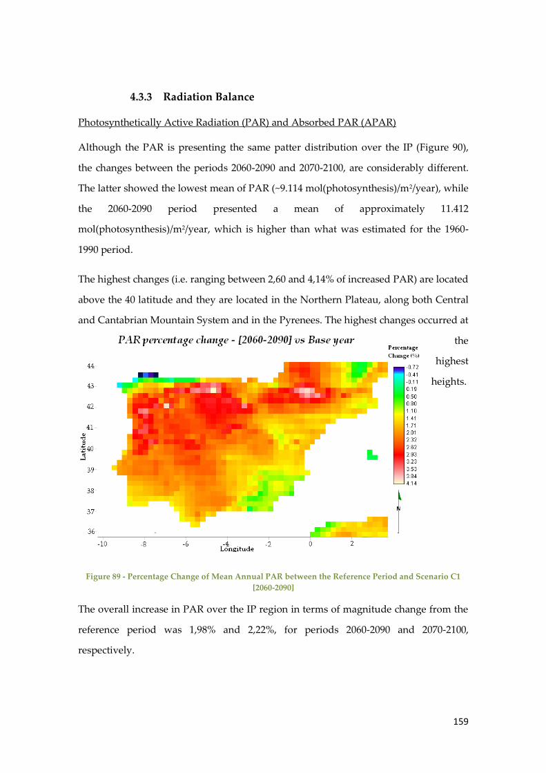
159

4.3.3 Radiation Balance

Photosynthetically Active Radiation (PAR) and Absorbed PAR (APAR)

Although the PAR is presenting the same patter distribution over the IP (Figure 90),

the changes between the periods 2060-2090 and 2070-2100, are considerably different.

The latter showed the lowest mean of PAR (~9.114 mol(photosynthesis)/m2/year), while

the 2060-2090 period presented a mean of approximately 11.412

mol(photosynthesis)/m2/year, which is higher than what was estimated for the 1960-

1990 period.

The highest changes (i.e. ranging between 2,60 and 4,14% of increased PAR) are located

above the 40 latitude and they are located in the Northern Plateau, along both Central

and Cantabrian Mountain System and in the Pyrenees. The highest changes occurred at

the

highest

heights.

Figure 89 - Percentage Change of Mean Annual PAR between the Reference Period and Scenario C1

[2060-2090]

The overall increase in PAR over the IP region in terms of magnitude change from the

reference period was 1,98% and 2,22%, for periods 2060-2090 and 2070-2100,

respectively.

160

One of the likely explanations for the increase in those areas might be linked to the

changes in mean annual evapotranspiration, due to the lower water available cause by

lower precipitation rates. The less water vapor (and therefore clouds) in the

atmosphere will enable a higher rate of solar radiation to go toward, which could

explain as well the boosting temperatures earlier verified for this area. Similarly to

what happen with the PAR variable, the same pattern of APAR remained for the

simulations of the four future scenarios. There were very small changes between the

scenarios and the

reference period, –

and between the

future scenarios

themselves. As it

can be seen from the

Figure 90, the

changes are barely

perceived.

For the scenarios C1 and E1, the mean absorbed PAR rate modeled by JSBACH was

~3.938 and 4.103 mol (photosynthesis)/m2/year by 2060-2090, respectively) and ~3.936

and 4.131 mol(photosynthesis)/m2/year (for the scenarios C2 and E2).

Figure 90 - Mean Annual APAR during Scenarios

C1 and Scenario E1 [2060-2090]

161

Furthermore, within the Scenarios “C”, the minimum APAR values have decreased

while the maximum values have increase from the reference period to the scenario C1,

and slightly decrease from scenario C1 to scenario C2. Conversely, the Scenarios “E”,

disclosed an increase of maximum values and an increase between the maximum from

reference period to scenario E1, and a decrease from scenario E1 to scenario E2.

In what concerns the distribution pattern of the difference of APAR between the

scenarios E1 and E2 and the reference period in means of percentage change, the

following images (Figure 92) shows the spatial and quantitative percentage changes.

Both scenarios were estimated to undergo positive and negatives changes i.e. to have

increases and reductions of absorbed PAR rates at different places. As such, the

Scenario E1 shows changes ranging between approximately -16 and 36%, while for the

Scenario E2, this range becomes a bit wider: -20 to 38% of change compared to the

reference period.

Figure 91 -Histograms and Statistical Analysis of Mean Annual APAR during Scenarios C1, C2, E1 and E2

162

The areas with higher positive changes (assigned to reddish areas) lie in northern

regions of the Peninsula, as well as in the regions of South Portugal and Alentejo

region in the same country.. For the negative percentage changes, i.e. decrease in

APAR rates, the greenish areas are spread all over the Peninsula, although the highest

decreases are likely to occur in three different spots across the boundary between

Portugal and Spain (dark and light blue areas).

Hence the model has simulated a small decrease of the mean value (~-1%) for the

scenarios admitting constant atmospheric CO2.concentration. For the scenarios E1 and

E2, the change of APAR was positive and a bit higher (~3 and 4%, respectively).

Figure 92 - Percentage Change of Mean Annual APAR between the Scenario E1 and E2

and the Reference Period

163

Reference period The different behaviors of APAR tendency in scenarios “C” and “E”

is likely to be the result from an increase of vegetation productivity (since the higher

the rate of production, the higher the photosynthetically processes, and hence, the

higher the solar radiation absorbed). Although this issue will be carefully addressed in

forthcoming chapter.

4.4 Carbon Balance Analysis– Future Scenarios

The approach made to the variables belonging to the carbon balance (GPP, NPP and

biomass) is similar to the one made when assessing changes in climate and

environmental variables for the future scenarios. This chapter presents the assessment

of the spatial patterns and magnitudes of change (having the reference period as basis),

although it is empathized the role of carbon dioxide in those changes. Hence, this final

section aims to assess biomass and vegetation productivity response to changes in

climate variables (and how strongly are they correlated) and aims to understand and

quantify the effect of fertilization of CO2, i.e. to understand how this physical variable

is affecting vegetation – namely herbaceous and forest biomass.

The potential biomass (from herbaceous and forest resources) modeled by JSBACH

will also be addressed in means of energy source by computing the energy potentials

of biomass modeled by JSBACH assuming the most plausible scenario, i.e. assuming

the increase of atmospheric CO2 concentration (and the climate change scenario A1B),

under different approaches assuming different politic and management of resources.

164

4.4.1 Gross Primary Production (GPP)

The maps projected by JSBACH regarding the Gross Primary Production for both

constant and changing atmospheric CO2 scenarios present the same pattern

distribution as in Figure 52. The average productivity as well as the maximum and

minimum GPP values vary considerably between each other, as well as between the

GPP estimated during the reference period. According to the results from the model,

during the scenario C1, in general, the GPP decreases its rates values (Figure 94). The

mean annual GPP decreases hence from 4.422 to ~4.007 g(CO2)/m2/year. The actual

maximum for this scenario is ~8.764 g(CO2)/m2/year and the actual minimum modeled

was~715 g(CO2)/m2/year.

Figure 93 - Mean Annual GPP during the

Scenario C1 [CO2] = 296 ppm (top) and during the

Scenario E1 [CO2] = 556 pm (botom)

165

Conversely to what JSBACH modeled for the Scenario C1, the Scenario E1 presents a

different trend on GPP change – instead of decreasing, it increases substantially.

Hence, the mean productivity projected for a scenario admitting and increase by 88%

of atmospheric CO2 concentration is ~5.575 g(CO2)/m2/year. The actual maximum and

minimum estimated change considerably as well: ~12.456 and 1.131 g(CO2)/m2/year,

respectively (Figure 95).

As it can be perceived from the Figure 96, the greatest differences occurred at higher

latitudes – approximately above the latitude 40 and associated to topographic features

– namely associated to the mountain ranges presented in the territory.

Figure 95 - Histograms and Statistical Analysis of GPP during the Future Scenarios C1, C2, E1 and #E2

Figure 96 - Mean Annual GPP differences between Scenario E1 [C02]=556ppm and

Scenario C1[C02]=296ppm

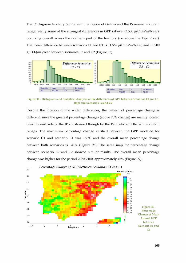
166

The Portuguese territory (along with the region of Galicia and the Pyrenees mountain

range) verify some of the strongest differences in GPP (above ~3.500 g(CO2)/m2/year),

occurring overall across the northern part of the territory (i.e. above the Tejo River).

The mean difference between scenarios E1 and C1 is ~1.567 g(CO2)/m2/year, and ~1.700

g(CO2)/m2/year between scenarios E2 and C2 (Figure 97).

Figure 94 - Histograms and Statistical Analysis of the differences of GPP between Scenarios E1 and C1

(top) and Scenarios E2 and C2

Despite the location of the wider differences, the pattern of percentage change is

different, since the greatest percentage changes (above 70% change) are mainly located

over the east side of the IP constrained though by the Penibetic and Iberian mountain

ranges. The maximum percentage change verified between the GPP modeled for

scenario C1 and scenario E1 was ~83% and the overall mean percentage change

between both scenarios is ~41% (Figure 95). The same map for percentage change

between scenario E2 and C2 showed similar results. The overall mean percentage

change was higher for the period 2070-2100: approximately 45% (Figure 99).

Figure 95 -

Percentage

Change of Mean

Annual GPP

between

Scenario E1 and

C1

167

The considerably higher CO2 uptake was thus a result of elevated atmospheric CO2,

since it was the only variable changed between the two scenarios meaning that the

results yielded by JSBACH model are in accordance with several authors (e.g. Amthor,

1998; DeLucia et al., 1999; Schaphoff et al., 2006, and many others).

Hence, despite the overall decreases of water supply (through precipitation) expected

to occur within roughly almost a century, the fertilization effect was modeled by

JSBACH, since plants uptake more CO2 from the atmosphere – resulting in increased

yields. Moreover, taking in consideration the former results from evapotranspiration

(i.e. the decreasing tendency in evapotranspiration mean annual values), these results

are also corroborated by Kimball et al. (2002), whom have concluded that as a result of

CO2 fertilization – the stomatal conductance tend to decrease, leading to decreases in

evapotranspiration. Furthermore, Kimball et al.(2002) (along with many other authors,

such as Amthor, 1998; DeLucia et al., 1999; Schaphoff et al., 2006) have also depicted an

improvement of water-use efficiency (as a result from what was explained) – which

drawn even more interested to get this variable analyzed (in following chapter).

Changing Environmental Controls on GPP

From the correlation coefficients presented in Table 40, the relationship between mean

annual GPP and every variable climate (aside from mean annual temperature and

APAR), tend to get considerably stronger for future scenarios assuming elevated CO2

and constant CO2 levels – although during the later scenarios the increase of correlation

was more considerable. The mean annual temperature correlation with mean annual

Figure 96 - Histograms and Statistical analysis of percentage change of GPP in period 2060-2090 (left) and

2070-2100 (right)

168

GPP showed a slightly different trend: despite the relationship got stronger for future

scenarios, the relationship was stronger for scenarios of elevated CO2.The mean annual

APAR stands out, since it was the only variable which got less spatially correlated with

GPP for future scenarios (and even lesser for scenarios elevated CO2. Every

relationship kept the same signal than in the reference period for all climate variables

(Table 40).

Table 40 – Comparison of Correlation coefficients for GPP and Climate Variables during the Reference

Period and the Future Scenarios

Response

variable

Water Cycle Radiation

T P ET SWC PAR APAR

Ref. Period

GPP

-0.25 0.65 0.76 0.12 -0.36 0.81

C1 -0.40 0.73 0.88 0.32 -0.40 0.79

C2 -0.42 0.73 0.89 0.35 -0.41 0.79

E1 -0.42 0.68 0.84 0.23 -0.39 0.78

E2 -0.43 0.67 0.85 0.26 -0.39 0.78

Table 41 presents the correlation analysis related to the interannual variability of the

mean annual GPP to the climate variables, showing thus the relationship between the

interannual variability of GPP and climate change (under scenarios of elevated and

constant CO2 levels). GPP was highly and positively correlated with changing ET

(RC1=0,79 and RC2=0,80) and APAR (RC1=0,79 and RC2=0,78) variables for scenarios where

atmospheric CO2 rising is disregarded. For scenarios assuming elevated CO2, GPP stills

highly correlated with ET and APAR, although the relationships are less strong. These

findings, i.e. the strong influence of ET and APAR in the interannual variability of GPP

are in accordance with Liu et al. (2011).

169

Table 41 - Correlation coefficients for variability of GPP in response to varying climate variables

Δ SCENARIOS Response

variable

Water Balance Radiation

ΔT ΔP ΔET ΔSWC ΔAPAR ΔPAR

C1-Ref. Period

ΔGPP

-0.30 -0.02 0.79 0.15 0.79 0.02

C2- Ref. Period -0.30 0.05 0.80 0.11 0.78 0.00

C2-C1 -0.30 0.52 0.83 0.12 0.72 -0.05

E1- Ref. Period -0.47 -0.32 0.65 0.10 0.62 0.18

E2- Ref. Period -0.47 -0.27 0.65 0.08 0.61 0.20

E2-E1 -0.36 0.27 0.70 -0.07 0.73 0.06

Despite the fact that mean annual precipitation has a great impact on the interannual

variability of primary production (Liu et al., 2011), this variable is not equal to water

available to vegetation. For that reason, the changing precipitation events throughout

the future scenarios and the reference period shown to be poorly and negatively

correlated under both “E” and “C” scenarios (although GPP was fairly more sensitive

to changing mean annual precipitation under scenarios of elevated CO2).

The negligible R computed for mean annual PAR suggests that GPP has a null

relationship with changing mean values of PAR. The almost absent relationship could

be due the fact that this variable does not go under considerable changes. Conversely

to APAR, SWC is subject of considerable changes although there is also an almost null

relationship with GPP (which can be explained as well by the same reason given for

weak correlation between mean annual precipitation and mean annual GPP). The

graphical correlation assessed in Table 40 and Table 41, are found in Figure 97 and

Figure 98. These graphics regard the variability between scenario C1 and the reference

period (i.e. 2060-2090/1960-1990), under scenarios assuming constant CO2 levels and

elevated CO2 levels (296ppm and 556ppm, respectively).

Among the variables composing the water balance, the correlation between

evapotranspiration and GPP resembles a linear correlation – the greater the values of

170

evapotranspiration variations between the scenario C1 and the reference period, the

greater the amount of GPP variability, i.e. evapotranspiration decrease, GPP also

decreases which shows its sensitivity to the variability of this climate variable. Both

precipitation and soil moisture (besides their lack of defined pattern), drove more

positive values for GPP (reflecting a greater increase in GPP during the [2060-

2090/1960-1990] period considered) for the scenario assuming rising CO2. (i.e. scenario

E1).

Figure 97 – Correlation between interannual variability of mean annual GPP and mean annual

variables from water balance (i.e. precipitation (top); evapotranspiration (middle); soil moisture content

(bottom) – between Scenarios E1 and C1 and Reference Period [1960-1990]

171

Similarly to the mean annual precipitation and mean annual soil moisture, both mean

annul temperature and PAR variables shown a similar tendency, (i.e. lack of pattern,

but a wider locations with increased GPP under the scenario E1). As expected the mean

annual APAR variability is likely linearly correlated with GPP Figure 98 .

Figure 98 - Correlation between interannual variability of mean annual GPP and mean annual

temperature (top) and variables from radiation balance (i.e. PAR (middle) and APAR (bottom) –

between Scenarios E1 and C1 and Reference Period [1960-1990]

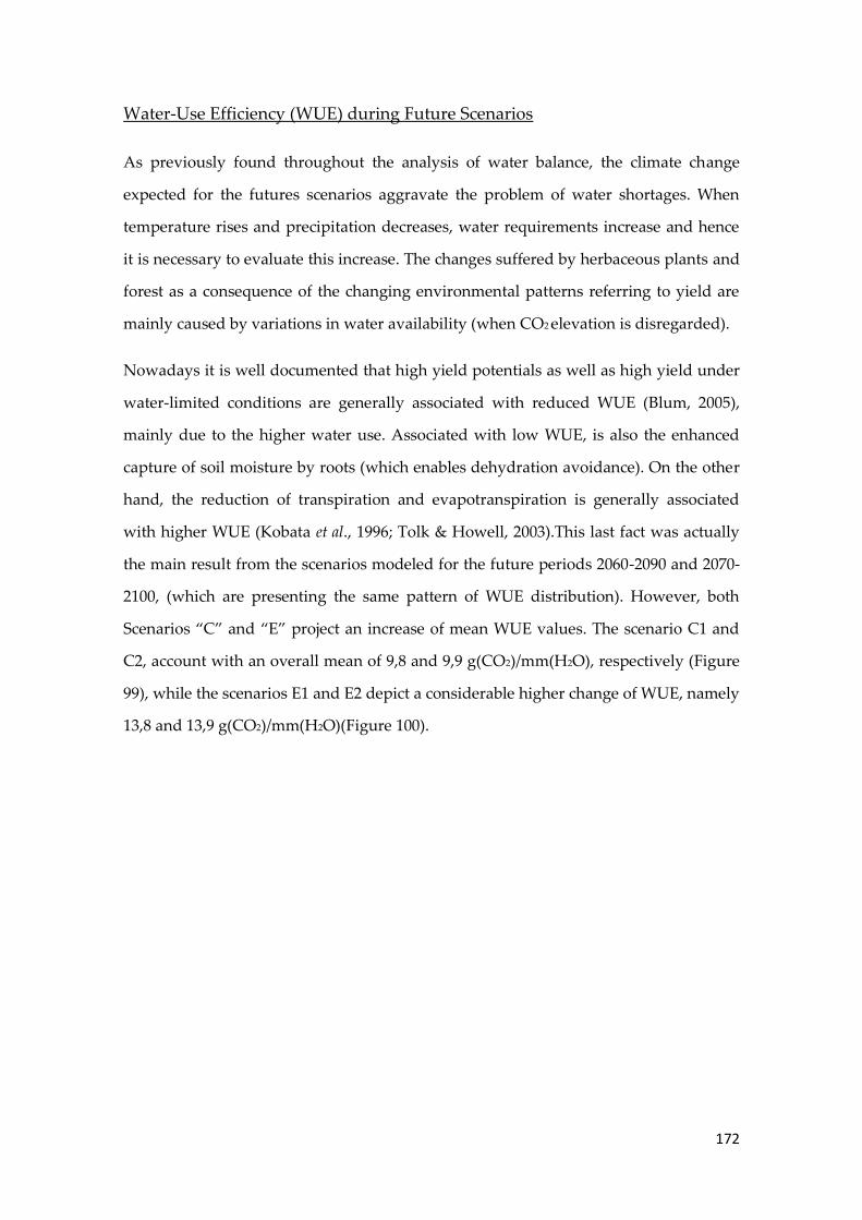
172

Water-Use Efficiency (WUE) during Future Scenarios

As previously found throughout the analysis of water balance, the climate change

expected for the futures scenarios aggravate the problem of water shortages. When

temperature rises and precipitation decreases, water requirements increase and hence

it is necessary to evaluate this increase. The changes suffered by herbaceous plants and

forest as a consequence of the changing environmental patterns referring to yield are

mainly caused by variations in water availability (when CO2 elevation is disregarded).

Nowadays it is well documented that high yield potentials as well as high yield under

water-limited conditions are generally associated with reduced WUE (Blum, 2005),

mainly due to the higher water use. Associated with low WUE, is also the enhanced

capture of soil moisture by roots (which enables dehydration avoidance). On the other

hand, the reduction of transpiration and evapotranspiration is generally associated

with higher WUE (Kobata et al., 1996; Tolk & Howell, 2003).This last fact was actually

the main result from the scenarios modeled for the future periods 2060-2090 and 2070-

2100, (which are presenting the same pattern of WUE distribution). However, both

Scenarios “C” and “E” project an increase of mean WUE values. The scenario C1 and

C2, account with an overall mean of 9,8 and 9,9 g(CO2)/mm(H2O), respectively (Figure

99), while the scenarios E1 and E2 depict a considerable higher change of WUE, namely

13,8 and 13,9 g(CO2)/mm(H2O)(Figure 100).

173

Figure 99 - Mean Annual WUE during scenario C1 (top)

and Scenario C2 (bottom)

174

The minimum WUE values have also increased in 2060-2090 (4,48 and 6,17

g(CO2)/mm(H2O), for scenarios C1 and E1, respectively) and slightly decreased in the

2070-2100 period (4,76 and 6,16 6,17 g(CO2)/mm(H2O) – scenarios C2 and E2,

respectively). The maximum values of WUE presented a similar tendency (máxWUEC1=

18,9; máxWUEC2=19,2; máxWUEE1=27,4; máxWUEE2=26,1 – all in g(CO2)/mm(H2O)).

In terms of magnitude of change in respect to the Reference period, the overall mean

WUE over the IP tend to increase by 6 and 7%, for the scenarios admitting constant

atmospheric CO2 concentration (for scenarios C1 and C2, respectively), whereas for the

for the scenarios E1 and E2, WUE greatly changes it tendency: it also increases but the

Figure 100 - Mean Annual WUE during scenario E1

(top) and Scenario E2 (bottom)

175

difference is substantial - 48 and 50%. Hence, comparing Scenarios “C” against

Scenarios “E”, the effect of rising atmospheric CO2 contributes to an increase of WUE

by 40% from scenario E1 to scenario C1 (within the 2060-2090 period), and 41% for the

2070-2100 period.

From these results, there is clear evidence that the CO2 elevation does have - within its

complex interactions with the water cycle and the productivity - a considerable

influence on water use efficiency. As it was previously explained for decreasing

evapotranspiration rates, this tendency of rising WUE levels is due, to the two changes

driven by atmospheric CO2 enrichment, i.e., the smaller stomata opening and lower

produce of stomata per unit of leaf area, which tend to reduce the rate of transpiration

whereas the amount of carbon hey gain per unit of water lost (i.e. the WUE) rises –

which will greatly increase their ability to withstand drought.

Other valuables explanations of how will the atmospheric CO2 enrichment improve the

relationship between plant and water, are (1) the increase of plant turgor: the leaf

osmotic potential is enhanced by leaf carbohydrate concentration, which is CO2

induced, and ultimately helps to maintain a proper leaf water content for continued

photosynthesis and growth – facing thus the decay of soil moisture availability); and

the (2) reduced water use (WU). Plants were designed by evolution to be cable of

controlling – and hence reduce the WU under drought stress. Moreover, even though

its genetics influence, when a plant is exposed to dry soil conditions, root morphology

and growth can change (i.e. increase under drought stress) to the extent that the

potential root length becomes irrelevant (Blum, 2005). One of the main reasons can rely

on the so-called “dehydration avoidance”, which is defined as the plant capacity to

sustain high cellular hydration under the effect of drought. This mechanism enables

that plant avoid dehydration by enhancing for instance the capture of soil moisture, by

limiting crop water loss, and also by retaining cellular hydration despite the overall

reduction in plant water potential (Blum, 2005).

Hence, regardless the CO2 variability, the overall water use efficiency of the Iberian

Peninsula tends to increase considering the climate changes modeled by JSBACH.

176

When the atmospheric CO2 elevation is taken into account the water-use efficiency

doubles its overall value. Which mean, that the increase of nearly 88% of the

concentration of dioxide carbon in the atmosphere, leads to a doubled biomass

production per unit of water. According to Emmrich (2007) the C4 grasses have higher

water-use efficiency (WUE) than do C3 shrubs, although on the other hand, the C4

plants are believed to lose this known advantage (Emmrich, 2007) due to the rising

atmospheric CO2 concentration. Even though, for that reason, the C4-grass-dominated

ecosystems are usually expected to present a higher WUE than C3-shrub dominated

ecosystems under same CO2 concentration and climatic variability (Emmrich, 2007).

Despite the previous findings it should be noticed that due to the multiple

environmental factors influencing the WUE and the complex relationship existing

between the carbon and water cycles, the spatial dynamics (as well as the variability

between each time period) should be addressed carefully (Tian et al., 2010). For

instance, WUE can be affected by soil fertility (which is linked to roots and water and

nutrients availability)(Stewart, 2001). Nevertheless, several studies corroborate these

results. In fact, Policy et al. (1993), have found results indicating that the increase in CO2

since the Glacial time to at the time (1993) CO2 concentrations have enhanced

biospheric carbon fixation by increasing the WUE of biomass production of C3 plants

(the bulk of the vegetation of the Earth). It also matches some other findings that

predict that an increase in atmospheric CO2 concentration is proposed to have an effect

on both the hydrological cycle and ecosystem productivity (Gelfand & Robertson, n.d.).

Light-Use Efficiency (LUE) during Future Scenarios

For the scenarios assuming constant atmospheric CO2 concentration, the light-use

efficiency tend to decrease contrarily to what happened with the scenarios E1 and E2,

where LUE shown to increase. Hence, the overall mean of LUE for scenarios C1 and C2

are projected to be ~1.00 and 0.98 g(CO2)/mol(photosynthesis)(Figure 101), representing

a decrease of -13 and -15%, respectively, from the reference period. This decrease

means that within these scenarios, there is a lower carbon uptake per unit of absorbed

photosynthetically radiation –which means that in order to produce the same amount

177

of carbons than during the reference period, there is a need of more ~13 and 15% of

APAR during the future scenarios (assuming that the other conditions maintains).

Figure 101 - Mean Annual LUE during Scenario

C1 (top) and Scenario C2 (bottom)

178

On the other hand, the scenarios E1 and E2 (Figure 102), depict increases of 26 and 28%

compared to the Reference period (meaning LUE values of 1.46 and 1.48, respectively).

Thereby, for the same amount of APAR, the vegetation over IP during these scenarios

produces more 26 and 28% of carbon.

Light-use efficiency was not greatly affected by the transition between the periods of

2060-2090 and 2070-2100, whether it was assumed a constant level of atmospheric CO2

concentration, or not. Hence, between the scenario C1 and C2, LUE resisted a decrease

of 2%, while for the scenarios E1 and E2 this difference was only 1%. Although the

magnitude of difference between scenarios “C” and “E” was considerable: between

Figure 102 - Mean Annual LUE during Scenario E1

(top) and Scenario E2 (bottom)

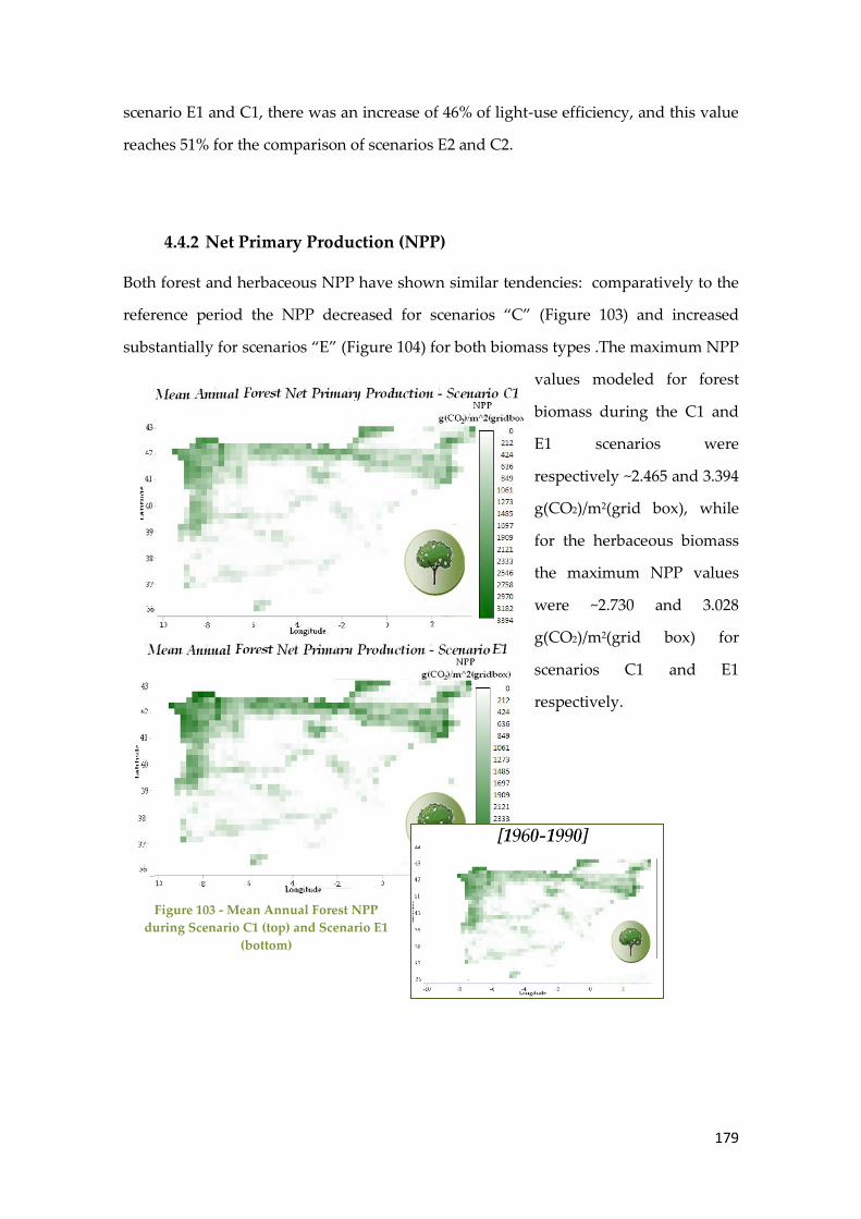
179

scenario E1 and C1, there was an increase of 46% of light-use efficiency, and this value

reaches 51% for the comparison of scenarios E2 and C2.

4.4.2 Net Primary Production (NPP)

Both forest and herbaceous NPP have shown similar tendencies: comparatively to the

reference period the NPP decreased for scenarios “C” (Figure 103) and increased

substantially for scenarios “E” (Figure 104) for both biomass types .The maximum NPP

values modeled for forest

biomass during the C1 and

E1 scenarios were

respectively ~2.465 and 3.394

g(CO2)/m2(grid box), while

for the herbaceous biomass

the maximum NPP values

were ~2.730 and 3.028

g(CO2)/m2(grid box) for

scenarios C1 and E1

respectively.

Figure 103 - Mean Annual Forest NPP

during Scenario C1 (top) and Scenario E1

(bottom)

180

Both biomass types had a considerable increment in the overall mean NPP. From the

scenario C1 to the scenario E1: herbaceous biomass’ NPP increased from 1.260 to 2.028

g(CO2)/m2(grid box), whereas for forest biomass it increased from 389 to 539

g(CO2)/m2(grid box).

The difference in both biomass types in means of percentage is shown in Figure 105.

The NPP underlying forest biomass verified more impact of CO2, as the maximum

Figure 104 - Figure 106 - Mean Annual Herbaceous

NPP during Scenario C1 (top) and Scenario E1

(bottom)

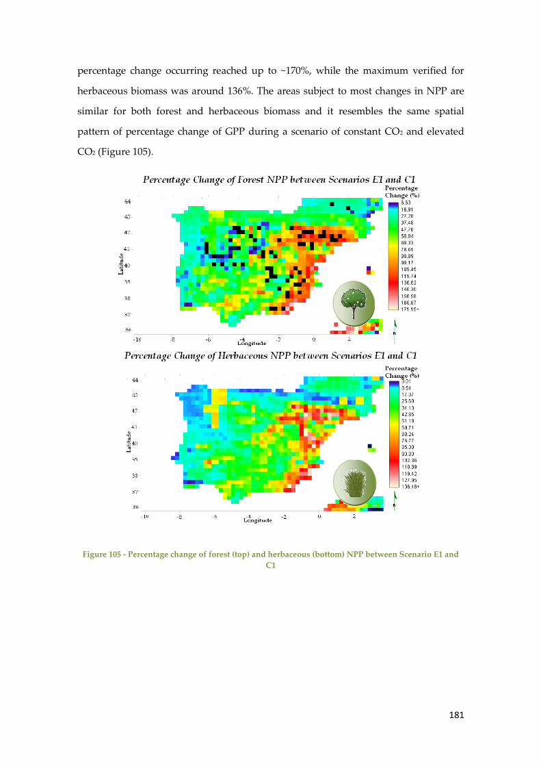
181

percentage change occurring reached up to ~170%, while the maximum verified for

herbaceous biomass was around 136%. The areas subject to most changes in NPP are

similar for both forest and herbaceous biomass and it resembles the same spatial

pattern of percentage change of GPP during a scenario of constant CO2 and elevated

CO2 (Figure 105).

Figure 105 - Percentage change of forest (top) and herbaceous (bottom) NPP between Scenario E1 and

C1

182

Figure 106 - Histograms and statistical analysis of Percentage Change of Forest (left) and Herbaceous

(right) NPP between Scenario E1 and C1

NPP and GPP interannual correlation

From the analysis of coefficient correlations (provided in Table 42) between the mean

annual NPP and the mean annual GPP (considering all biomass) over the IP during the

future scenarios, it is noticeable an increase of strength of the relationship of these two

variables in comparison to the reference period. The scenarios disregarding CO2 rise

are those where NPP and GPP are more correlated, although there is not a considerable

change between each period (i.e. 2060-2090 and 2070-2100).

Table 42 - Parson's coefficients between NPP and GPP over the IP, during Future Scenarios

SCENARIOS

Reference

Period C1 C2 E1 E2

Coefficient of Correlation”R” 0,88 0.91 0.92 0.89 0.89

Figure 107 also enables to understand (through the value of R2), that the NPP and GPP

relationship can be “more explained” as a linear relationship, as the regression line fits

better the correlation between these two variables. The considerable change in NPP

and GPP correlation might be linked to the response of autotrophic respiration to

climate change. This process is an important component of vegetation carbon balance

(as well as the CO2 budget), although so far the autotrophic respiration response to

increasing concentrations of CO2 in the atmosphere is not fully understood (Bunce,

2004).

183

Figure 107 - Regression analysis and coefficients of determination between NPP and GPP during

Future Scenarios

Comparison of results with other studies

The conclusions concerning productivity response to climate change in regions such as

Iberian Peninsula widely different from author to author. For instance, the IPCC (2001)

stated with a medium confidence14 that the increase of agricultural yields for most

crops as a result of increasing atmospheric CO2 concentration would be counteracted

by the risk of water shortage in southern and Eastern Europe, and hence this regions

would have decreases in productivity. These projections are supported by other

authors (e.g. Rost et al., 2009). On the other hand, Reyer & Gutsch (n.d.) stated that in

the Mediterranean forests, the effect of elevated concentration of atmospheric CO2 on

stomatal conductance, will lead to enhanced water-use-efficiency (which is consistent

with the findings present in section regarding the WUE during future scenarios)

resulting in increased productivity and biomass production. Reyer & Gutsch (n.d.) also

stated that despite the key limiting factors for each forest (such as temperature for

Temperate forests or water availability for Mediterranean forest), both biomes’

14

The authors of the report assign a confidence level that represents the degree of belief among the authors in the validity of a conclusion. A quantitative confidence level of 33-67%, was assigned to “medium confidence level”.

184

responsiveness to [CO2] reveal to be very consistent and positively related to

productivity and biomass changes.

Since despite the decreases in ET, rainfall and soil moisture, the productivity is

expected to increase considerably, perhaps we could assume that the JSBACH model

hence, attributes a considerable weight on CO2 fertilization (at least high enough to

offset the water scarcity conditions), comparatively to other studies.

4.4.3 Biomass Potentials for Future Scenarios

Both sets of herbaceous and biomass maps results provided by the JSBACH model,

have no visual expression in what concerns a perceptible change in aerial densities as

they look similar to the maps obtained in Figure 61 and Figure 62, respectively, and

hence they are not here disclosed Notwithstanding, the results of forest and

herbaceous biomass are significantly different in future scenarios when compared to

the reference period.

In terms of absolute biomass, the shares of forest and herbaceous biomass differed

from what was estimated for the 1960-1990 period (i.e. 78% and 22% for forest and

herbaceous biomass, respectively). For both scenarios C1 and C2, the contribution of

herbaceous biomass has decreased by 6% compared to the reference period, while the

forest biomass accounted with more of the same percentage for the overall biomass

over the IP. On the other hand, for the scenarios assuming elevated concentrations of

atmospheric CO2, the change in contribution of each biomass type to the overall

scheme just differed by 1% from the reference period (decreasing for herbaceous and

increasing for forest biomass) (Figure 108). In terms of absolute biomass values, these

values can be found in the table below (Table 43).

185

Figure 108 –Share of Herbaceous and Forest Biomass to the overall amount during Scenarios “C” (left)

and Scenarios “E” (right)

Table 43 –Absolute amounts of Forest and Herbaceous Biomass (tonnes) during the Future Scenarios

C1, C2, E1 and E2

C1 C2 E1 E2 “E” / “C”

FOREST

BIOMASS

7,46 x 108

(tones)

7,42 x 108

(tones)

8,68 x 108

(tones)

8,73 x 108

(tones)

16-17%

HERBACEOUS

BIOMASS

1,43 x 108

(tones)

1,36 x 108

(tones)

2,26 x 108

(tones)

2,25 x 108

(tones)

55-65%

The comparison between the forest biomass from the reference period and the futures

scenarios “C” and “E” discriminated by PFT (Figure 109), enable to understand that the

major differences occurred in temperate broadleaf deciduous trees and coniferous

evergreen trees. These two PFT showed a considerable increase in biomass in response

to elevation of CO2 levels, especially the latter, which biomass increased over

50.000.000 tonnes between the reference period and the both future scenarios E1 and

E2. The most significant difference in biomass from the reference period to the future

scenarios with constant CO2 levels occurred for the coniferous evergreen trees, which

verified a reduction by approximately 25.000.000 tonnes, whereas the remaining PFT

presented a considerably lower change (even though the temperate broadleaf

deciduous trees had an almost negligible increase).

186

Figure 109 – Comparison of Absolute Amounts of Forest Biomass between Reference Period and

Scenarios “C” (left) and between Reference Period and Scenarios “E”(right) segregated by PFTs

The amount of herbaceous biomass presented noticeable differences for the future

scenarios assuming constant CO2. All the four PFTs considered, shown decreases in

biomass (Figure 110), being the C3 crops the one most affected by the climate variables,

having decreases of approximately 40.000.000 tonnes. This PFT was also the most

affected by the variable CO2 concentration, showing as response to that, an increase of

~10.000.000 tonnes (from the reference period). The remaining PFT did not present

significant changes in their biomass: C4 grasses continued to present a decrease as in

the constant CO2 assumptions (although considerably lower), while the C3 grasses and

C4 crops have both presented small increases.

Figure 110 – Comparison of Absolute Amounts of Herbaceous Biomass between Reference Period and

Scenarios “C” (left) and between Reference Period and Scenarios “E”(right) segregated by PFTs

Since the scenarios “C” and scenarios “E” differ on the concentration of atmospheric

CO2, the comparison of biomass change between these scenarios enable to depict

187

differences between the responses of each PFT to the rising CO2 (since the climate

variables are assumed to be changing equally). The Table 44 shows the percentage of

change between the scenarios C1 and E1 and scenarios C2 and E2. All PFT (aside

deciduous shrubs) showed higher changes for the period 2070-2100 (i.e. between C2

and E2) than the period 2060-2090. The percentage changes of biomass forest and

herbaceous biomass between scenarios assuming constant CO2 and elevated CO2

concentrations, is disclosed in the Table 44 by PFT.

Table 44 Percentage of Change of Forest and Herbaceous Biomass between Scenarios “C” and

Scenarios “E” – Effect of rising CO2 levels

(%) CHANGE E1 vs C1 E2 vs C2

FOREST BIOMASS

Temperate broadleaf evergreen trees 11% 13%

Temperate broadleaf deciduous trees 22% 23%

Coniferous evergreen trees 13% 14%

Rain green shrubs 13% 15%

Deciduous shrubs 5% 5%

HERBACEOUS BIOMASS

C3 grass 41% 45%

C4 grass 52% 61%

C3 Crops 69% 79%

C4 Crops 67% 76%

The PFT from forest biomass with higher impacts of elevated CO2 were the temperate

broadleaf deciduous trees, followed by rain green shrubs, coniferous evergreen trees,

temperate broadleaf evergreen trees and finally deciduous shrubs. By 2060-2090 (C1),

approximately 22% of the deciduous forest growth could be attributed to the variation

in CO2 – whereas for deciduous shrubs only 5% of its biomass increase resulted from

that.

A possible reason for these tendencies showing different sensitivity of these forests to

CO2 change, could rely on the type and structure of the ecosystem. The results are in

accordance with many authors (e.g. Hui et al., 2003; Richardson et al., 2007)), since their

studies have ordered the decrease of impact on forest in the following way: deciduous

forest, mixed forest, coniferous and peat land – although they refer to environmental

changes in general (not highlighting the solely effect of CO2). For that reason the

188

findings disclosed in Table 44 should not be compared straightforwardly with the later

studies.

Herbaceous biomass showed to be highly CO2-responsive. The PFTs with higher

responses were by order, C3 crops, C4 crops, C4 grasses and C3 grasses. Typically C3

plants are responding better to atmospheric CO2 increasing, due to the CO2 saturation

effect on C4 leaves . For instance Wand et al. (1999) estimated biomass enhancements of

44 and 33%, respectively, for C3 and C4 plants for a doubling atmospheric CO2

concentration; while Poorter (1993) and Wand et al. (1999) concluded that on average

the growth stimulation of C4 plants in response to a doubling ambient CO2 was about

22-33%, compared with 40-44% for C3 plant. Those studies do not correspond to the

findings on Table 44: firstly, the increases in biomass (where CO2 almost reaches the

doubling concentrations from the reference period) present at the table are

considerably higher, and the other noticeable difference regards the grasses response

(i.e. C4 grasses were more sensitive to CO2 than C3 grasses).

An advantage that may come to C4 grasses (explaining their enhanced CO2-

responsiveness compared to C3 grasses), could be the fact that the ongoing rise in the

air (which was verified in ) enhances the ability of C4 grass to increase its uptake for

some nutrients (BassiriRad et al. ,1998). Moreover, Poorter (1993) and Wand et al. (1999)

concluded that the magnitude of the growth stimulation of C4 plants to elevated CO2

increases with decreasing soil water availability. Therefore, those results and the

findings in Table 44 cannot be considered mutually exclusive in terms of final

conclusions (since SWC is projected to decrease Figure 43 and Figure 84). In fact, Wand

et al. (1999) suggested that under water-stress conditions, C4 species end up to be more

competitive than C3 – which in fact characterize the region in the IP where this

conditions are more likely to occur (as can be compared from Figure 26 and Figure 84).

Many authors (e.g. Berry & Downton, 1982; Cure & Acock, 1986), generally assumed

that C4 plants do not respond to elevated CO2 under well-watered conditions. C4

plants are known to better cope with water stress (Wand et al., 1999), which may be the

reason why Campbell et al. (2000) concluded that the growth of C4 species in

grasslands is more responsive to CO2 concentration than C3 species.

189

The magnitude of biomass change (i.e. values and patterns) is different between forest

biomass and herbaceous biomass meaning that they have different responses to

changes in climate variables and atmospheric CO2 levels. For the 2060-2090 period,

forest biomass showed considerable changes between scenarios C1 and E1, and it

present higher values for the later scenario. The highest changes (ranging between

approximately 70 and 100%) occur in several areas located along the eastern region of

Spain as it can be depicted from the map (Figure 111).

The

green colored area existing evenly along the entire north of Spain (green zone), shows

that the forest biomass located at the Temperate zone responded with increases of 20-

30% to the elevation of CO2. The central and southeastern of the IP shows very low

percentage changes, lower than 6%. The mean percentage change of biomass response

to elevated CO2 is 23%. The pattern and magnitude change between scenarios C2 and

E2 had similar results), although the overall percentage increase is higher (~25%)

(Figure 112).

Figure 111 – Percentage of Change of Forest Biomass between Scenario E1 [CO2]=556ppm and

Scenario C1 [CO2]=296ppm

190

The results of magnitude of change of herbaceous biomass between a scenario of

elevated and constant atmospheric CO2 was considerably greater than in the previous

case. The pattern also seems to be smoother between percentage changes. Almost the

entire territory of Portugal verified percentage changes smaller than 7% between

scenarios C1 and E1 (Figure 113) as well as the Temperate zone (aside from that area

coming inwards from the northern shore (close to Asturias) which has presented lower

SWC and evapotranspiration values (Figure 43 and Figure 45)). In this area (as well in

the southeast shore and Aragón and Cataluña regions) JSBACH modeled a change by

over 215% of herbaceous biomass. In some areas, this biomass type has reached over

500% of percentage of increase (between a scenario of constant and elevated CO2 levels.

Figure 113 - Percentage of Change of Herbaceous Biomass between Scenario E1 [CO2]=556ppm and

Scenario C1 [CO2]=296ppm

The overall mean of increase in herbaceous biomass for a elevated CO2 scenario for the

period 2060-2090 was around 89%, although the values of percentage increase more

common ranged around 30% (Figure 114). The map of percentage change of

Figure 112 – Histograms and Statistical Analysis of Percentage Change of Forest Biomass between

Scenarios E1 and C1 (left) and between Scenarios E2 and C2 (right)

191

herbaceous biomass between scenarios E2 and C2 had similar results (and for that

reason they are not here disclosed). The herbaceous biomass of IP for the period 2070-

2100, showed an overall mean of ~100% increase of biomass as a response to elevated

atmospheric CO2 concentration (Figure 114).

Figure 114 - Histograms and Statistical Analysis of Percentage Change of Herbaceous Biomass between


In terms of percentage change of all biomass across the IP between the scenarios

assuming constant and elevated CO2 levels, the set of all PFT has presented an increase

of biomass for the later scenarios (Figure 115). The map for the percentage change

between scenarios E2 and C2 has presented a similar pattern.

Figure 115 - Percentage of Change of Total Biomass between Scenario E1 [CO2]=556ppm and Scenario

C1 [CO2]=296ppm

The map above, is considering both biomass types together and for that reason the

overall mean percentage change of biomass is higher than when considering solely

192

forest biomass and lower than considering only herbaceous biomass, i.e. ~49% (Figure

116). For the period 2070-2100, this value reaches up to ~56%.

Figure 116 - Histograms and Statistical Analysis of Percentage Change of Total Biomass between


4.5 Biomass Response to Climate Change

This section aims to understand how changing climate variables are projected to affect

both forest and herbaceous biomass changes under scenarios with constant CO2 and

elevated CO2 levels. Table 45 presents the correlations coefficients between the

variation of each climate variable and the variation of biomass density (in gC/m2) (this

variation regards changes between future scenarios and the reference period). The

stronger correlations (i.e. R >0,4) are highlighted in bold).

Table 45 - Correlation coefficients between Changing Biomass and Changing Climate Variables

Scenarios Biomass Climate variables

ΔFOREST

ΔT ΔP ΔET ΔSWC ΔPAR ΔAPAR

Constant

CO2

C1[2060-2090] – Ref 0,13 0,11 0,38 -0,02 0,03 0,44

C2[2070-2100] – Ref 0,11 0,13 0,39 -0,04 0,00 0,44

Elevated

CO2

E1[2060-2090 ]– Ref -0,37 -0,07 0,53 0,18 -0,11 0,49

E2[2070-2100 ]– Ref -0,36 0,00 0,52 0,20 -0,06 0,45

ΔHERBACEOUS ΔT ΔP ΔET ΔSWC ΔPAR ΔAPAR

Constant

CO2

C1[2060-2090] – Ref -0,51 -0,04 0,77 0,21 -0,0041 0,58

C2[2070-2100] – Ref -0,51 0,02 0,76 0,21 -0,02 0,55

Elevated

CO2

E1[2060-2090 ]– Ref -0,10 0,27 0,39 0,00 -0,03 0,31

E2[2070-2100 ]– Ref -0,10 0,30 0,38 -0,03 -0,11 0,31

Forest biomass presents stronger (and positive) relationships with APAR and

evapotranspiration and these relationships are likely to become even stronger under

193

scenarios assuming the CO2 fertilization effect. On the other hand, the strongest

responses of herbaceous biomass occur for changes in ET, APAR and temperature

(having a negative relationship with the later) and these variables are (conversely to

forest biomass) considerably stronger under scenarios assuming constant CO2 and the

impact of changing precipitation, SWC and PAR on herbaceous biomass trend is,

according to the model, negligible. Figure 17 and Figure 118 illustrate the correlation

between variation of each biomass type and variations in climate variables - between

the period 2060-2090 and the reference period, and under scenarios of constant and

rising CO2 levels (scenarios C1 and E1, respectively).

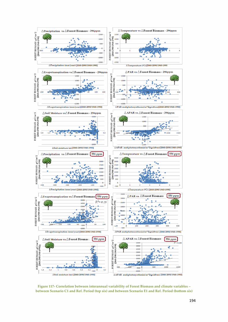
194

Figure 117- Correlation between interannual variability of Forest Biomass and climate variables –

between Scenario C1 and Ref. Period (top six) and between Scenario E1 and Ref. Period (bottom six)

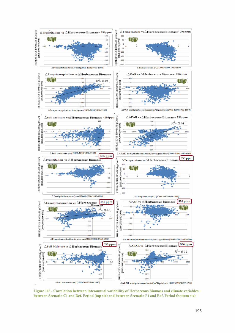
195

Figure 118 - Correlation between interannual variability of Herbaceous Biomass and climate variables –

between Scenario C1 and Ref. Period (top six) and between Scenario E1 and Ref. Period (bottom six)

196

Regarding firstly the responses of biomass to warming temperature, herbaceous

biomass presented in stronger correlation between its interannual variability and

interannual change in temperature for scenarios of constant CO2 levels. The correlation

present in the top right graph in Figure 118, roughly resembles a linear relationship.

Forest biomass shows no pattern for scenarios of constant CO2 levels, justifying the

negligible correlation between it and temperature (R=0,13). For scenarios of elevated

CO2 the response of interannual variability of forest biomass to warming temperatures

suffers a considerably shift as it can be depicted form the Figure 120 – where data

points above the line illustrates a positive response to warming temperatures.

In what concerns the water balance variables (i.e. precipitation, evapotranspiration and

soil moisture), as excepted from previous results for impact of climate variables in

GPP, the graphs showing the correlation between these variables showed no

resembling pattern with exception to the evapotranspiration, which presented a

roughly linear shaped pattern. However, the only significant determination coefficient

was assigned to the relationship between changing herbaceous biomass and changing

evapotranspiration for scenarios assuming constant CO2 (R2 = 0,59). Despite the

negligible correlations with soil moisture, both forest and herbaceous biomass, showed

to be more responsive to smaller decreases in soil moisture (i.e. around -0,2m of SWC),

although herbaceous were more negatively affected, by decreasing its biomass whereas

forest showed mostly increases.

The responses to the variable PAR, lacked a traceable pattern for responses of both

forest and herbaceous biomass. From the graphs present in Figure 117 (third graph

from the right top, and bottom right graph), for positive change in APAR, the response

of forest biomass seems to be roughly linear (although its determination coefficients R2

negligible). Herbaceous biomass presented higher R2 (although very small), since its

interannual variability shows a smooth linear relationship with interannual variability

of APAR (Figure 118).

197

4.6 Biomass energy Potentials

As described in methodology, the assessment of biomass energy potentials was

conducted under two distinct approaches: “Max Potentials” consisting in the

estimations of forest biomass energy potential derived from clear cuttings activities

and “Plausible Potentials”, a more realistic approach assuming several scenarios of

forest and herbaceous residues use for energy purposes.

Max potential

The “Max Potential” approach was broken at the level of some PFT (or group of PFT)

depending on being or not subject of interest to be analyzed. The main results can be

found in Table 46:

Table 46 –Biomass and Herbaceous Energy Potential from Clear Cutting activities (Max Potential) for

all scenarios

BIOMASS

TYPE

PFT CONVERSION

PATHWAY POTENTIAL ENERGY (EJ)

Ref. C1 C2 E1 E2

FOREST

BIOMASS

(Clear

cutting)

ALL* Combustion 3,362 3,289 3,274 3,828 3,850

Gasification 4,706 4,604 4,583 5,359 5,389

Temperate Broadleaf

Deciduous Trees

Combustion 1,333 1,345 1,346 1,639 1,656

Gasification 1,866 1,883 1,884 2,295 2,318

Coniferous evergreen trees Combustion 1,868 1,796 1,783 2,023 2,029

Gasification

2,616 2,515 2,496 2,833 2,840

*ALL = “All” stands for all the PFT belonging to the biomass type.

The coniferous evergreen trees consist in the PFT accounting with more energy

potential, followed by the temperate broadleaf deciduous trees. As expected from the

earlier assessment of biomass potential for scenarios C and E, the later present a

considerable rise in energy potential when compared to the reference period or

scenarios disregarding elevated CO2. As a result from rising atmospheric CO2

concentration, the energy potential from a “max potential” perspective increase by 13%

from the reference period – and decreases by 2% when CO2 is assumed to remain

constant (Figure 122), considering all forest biomass (i.e. all PTF are accounted).

198

Figure 119- Percentage Change of Biomass Energy Potential from Forest Biomass under a "Max

Potential" approach

The energy potential assessment made through the Max Potential shows that the forest

of the Iberian Peninsula contain an overall mean energy potential of approximately 3,8

EJ for the scenario E1 (when assuming combustion as the conversion pathway).

Plausible Potentials

The biomass energy potential assessment (within a plausible approach) is presented in

Table 47, regarding only the scenarios E1 and E2 since they represent the most

probable future conditions (in regard of climate variables as well atmospheric CO2

concentration)(similar tables regarding the results achieved for reference period and

scenarios C1 and C2 can be found in Appendix B). The forest residues were accounted

separately, in order to avoid double-counting of residues from both activities (i.e.

thinning and logging). The energy potentials do not verify a great change between the

periods 2060-2090 and 2070-2100. Within the forest biomass group, the PFT comprising

shrubs, had the lowest contribute to overall results while the temperate broadleaf

deciduous trees and coniferous evergreen trees accounted for most of the total result.

The herbaceous biomass has a much lower energy potential due to its considerable

lower biomass potential (even though this biomass produces a higher amount of

residue per unit of biomass). The crops are among the herbaceous biomass, the PFT

with higher energy potential once again due to its greater biomass potential along with

its higher LHV value.

199

Table 47- Plausible approach results for Forest and Herbaceous Biomass under scenarios assuming

climate change and elevated CO2

RESIDUE REMOVAL

SCENARIO

BIOMASS

TYPE

SOURCE PFT

ENERGY POTENTIAL (EJ)

SCENARIO E1 SCENARIO E2 Combustion Gasification Combustion Gasification

BAU

(10%)

FOREST

RESIDUES

(Top and

branches from

thinning)

All 0,041 0,058 0,041 0,058

T. B. Deciduous Trees 0,018 0,025 0,018 0,025

C. evergreen trees 0,022 0,031 0,022 0,031

LOW-YIELD

(20%)

All 0,082 0,115 0,083 0,116



HIGH-

YIELD

(40%)

All 0,165 0,231 0,166 0,1232

T. B. Deciduous Trees 0.071 0,099 0,071 0,100


BAU

(10%)

FOREST

RESIDUES

(Logging

residues)

All 0,124 0,173 0,124 0,174



LOW-YIELD

(20%)

All 0,247 0,346 0,249 0,348



HIGH-

YIELD

(40%)

All 0,495 0,693 0,498 0,697



BAU

(10%)

HERBACEOUS

RESIDUES

(Straw from

agriculture)

All 0,086 0,121 0,086 0,121

C3 and C4 grass 0,037 0,051 0,037 0,051

C3 and C4 crops 0,050 0,070 0,050 0,070

LOW-YIELD

(20%)

All 0,173 0,242 0,173 0,242

C3 and C4 grass 0,073 0,103 0,073 0,102

C3 and C4 crops 0,099 0,139 0,099 0,139

HIGH-

YIELD

(40%)

All 0,346 0,484 0,345 0,483

C3 and C4 grass 0,147 0,206 0,146 0,205

C3 and C4 crops 0,199 0,279 0,199 0,278

Comparison with other studies

Table 48 contains results of energy potentials from forest and agricultural residues

estimated for the Iberian Peninsula from four studies. The first one was conducted by

CRES (Nikolau et al., 2003), the second by the European Environment Agency (EEA,

2006); the third by the RENEW project and the last and more recent one by CHRIGAS

(Esteban et al., 2008; Esteban et al., 2010). Despite the use of the same LHV values, the

several studies should not be straightforwardly compared due to the lack of

information on the methodology followed in most of the works and production values

used for the crops involved. Moreover, different time periods are being regarded. In

order to compare more proximate results from this dissertation, the table is presenting

200

the results obtained from biomass residues available during the reference period, since

the amount of biomass available then is likely to be similar to the studies (instead of the

future biomass potentials where CO2 has enhanced further biomass generation). This

table serve hence as a raw approach to the evaluation of the reliability of the achieved

results.

Table 48 - Comparison between assessments on biomass resources (data in EJ/year) estimated by other

authors and for the reference period

FOREST RESIDUES Authors Energy Potential (EJ)

Nikolau et al. (2003) 0,126

EEA (2006) 0,081

RENEW (n.d.) 0,068

Esteban et al. (2010) 0,103

Aparício (2012)

Results from: Reference Period [1960-1990]

Conversion Pathway: Combustion

SCENARIOS Thinning Logging

BAU 0.036 0.109

LOW-YIELD 0.072 0.217

HIGH-YIELD 0.142 0.435

AGRICULTURAL RESIDUES Authors Energy Potential (EJ)

Nikolau et al. (2003) 0,150

EEA (2006) 0,392

RENEW 0,128

Esteban et al. (2010) 0,266

Aparício (2012) SCENARIOS Agriculture

Results from: Reference Period [1960-1990]

Conversion Pathway: Combustion

BAU 0,082

LOW-YIELD 0,164

HIGH-YIELD 0,327

Concerning forestry, in the present work the values obtained for the available biomass

assuming the BAU scenario are generally lower than the obtained by other authors. For

LOW-YIELD scenarios, the energy potential assessed for the reference period is in the

range of the other studies, whereas for HIGH-YIELD scenarios the results from are

considerably higher (which is fairly reasonable, since the removal rates assumed in

HIGH-YIELD were not applied in Iberian Peninsula at the time that the other studies

were developed). Generally, these comparisons state the reasonability of the

estimations achieved at the present work.

203

5 Conclusions

The goals stated for this work include: (1) the understanding of the magnitude of the

impact that climate changes and the solely effect of rising CO2 (in accordance to the

prescribed in A1B scenario from IPPC) have in biomass and productivity over the

Iberian Peninsula (IP), by (2) modeling the interannual variability in terrestrial

productivity and biomass across de region (having the period 1960-1990 as reference)

depicting from there (3) the energy potentials derived by biomass in future scenarios

(2060-2090 and 2070-2100 periods). The carbon fluxes were modeled by JSBACH model

and its results were handled using GIS and statistical analysis. A better understanding

of the applicability (and reliability) of this model on achieving the latter stated goals

was gained (by comparisons of some results with other authors), reaching this way

another goal purposed in this work. This chapter presents the main conclusions

achieved regarding those goals.

5.1 Climate change and CO2 fertilization impact on productivity and biomass

The scenarios “E1” and “E2” (2060-2090 and 2070-2100 periods, respectively) were

modeled taking into account the CO2 fertilization effect while scenarios “C1” and “C2”

(2060-2090 and 2070-2100 periods, respectively) kept atmospheric CO2 constant at 296

ppm. In the latter case, productivity changes were only driven by the modeled changes

in climate variables, whereas the first case the full effect of changes in temperature,

precipitation and atmospheric CO2 level is taken into account.

204

According to the JSBACH model, most regions experience significant increases in

productivity (GPP and NPP) under assumed CO2 fertilization, while for scenarios

disregarding elevated CO2 the productivity and biomass were modeled to decrease

(although not as significantly as in scenarios of elevated CO2). The Temperate Zone

presented considerably higher productivity rates comparatively to the Mediterranean

zone, due to the greater concentration of forest biomass in the first. Although the

spatial distribution of changes in GPP, NPP and biomass across the IP are very similar,

(i.e. higher changes were modeled to occur in the eastern and southeastern quadrant of

the region), the magnitude of change varied considerably among these three variables.

The comparison between “E” and “C” scenarios enabled the understanding of the

magnitude of the impact that roughly doubling the CO2 from 296ppm to 556 ppm and

to 598ppm (scenario E1 and E2, respectively) had on productivity. The GPP had an

overall mean annual increase by ~41 and ~45% across the IP, whereas forest biomass

NPP increased by ~54% and herbaceous biomass NPP by ~36% (between scenarios E1

and C1. In what concerns to the percentage change in forest and herbaceous biomass,

Figure 120 illustrates the changes between future scenarios and the reference period, as

well as the change in biomass between scenarios assuming constant CO2 and scenarios

accounting with rising CO2.

Figure 120 – Comparison of Forest and Herbaceous Biomass changes between futures scenarios and

reference period (left) and between elevated atmospheric CO2 concentration scenarios (E1 & E2) and

constant atmospheric CO2 concentration (C1 and C2) (right)

205

The climate variables affecting productivity were mostly APAR, followed by

evapotranspiration (ET) and precipitation, whereas forest biomass shown to be more

affected by APAR, followed by precipitation, ET and temperature. Another major

difference was the greater susceptibility of herbaceous biomass to increased

temperature (which showed a moderate negative response) under constant CO2

scenarios, while for forest biomass this correlation was less strong, and positive, under

elevated CO2 scenarios. Despite that, generally the JSBACH model did not enabled to

understand the relationship between environmental factors and herbaceous biomass,

since the correlations achieved among them were mostly negligible, which could be

interpreted as one limitation of the model. Scenarios “C” and “E” also presented

differences concerning how productivity (and biomass) were related with climate

variables, and how strongly is the variation productivity affected by the variation of

climate. GPP showed to be strongly correlated with climate variables for scenarios of

constant CO2, although GPP interannual variation shown to be strongly affected by ET

and APAR changes.

The water-use efficiency (WUE) increased for both futures scenarios “C” and “E”

comparatively to the reference period. However, the increase verified for elevated CO2

scenarios was considerably higher than the for constant CO2 scenarios (WUE > 58%

and WUE > 7%, respectively). This rise in WUE explains the great increase in

productivity. On the other hand, the light-use efficiency (LUE) decreased for scenarios

“C” (LUE< -13%) and increased considerably for scenarios “E” (LUE > 28%). Although

WUE tendencies were in accordance with multiple authors, the findings concerning the

increase of productivity as a result of the CO2 fertilization effect over the IP, were not in

accordance with multiple authors that predicted instead, lowering productivity rates

for the region as a consequence of water shortage driven by climate change.

Henceforth, it has to be noted that the beneficial effect of CO2 fertilization is subject to

heavy debate, specially taking into account that the model (comparatively with other

research results, is considerably overestimating the effect of CO2 fertilization), since the

IP region is stated as being water-limited and the decrease in water supply (for rising

206

CO2 scenarios) is not evidently affecting productivity and biomass growth. On the

other hand, besides the assessment of carbon fluxes, the modeled output climate

variables (i.e. ET, APAR and soil moisture) enabled to assess the model in what

concerns its applicability to projected climate variables (as these results were compared

with other authors which considered as well the A1B scenario). Hence, based on these

comparisons, the JSBACH model showed an acceptable reliability.

5.2 Biomass Energy Potentials

Under a scenario of elevated CO2 (the likely trend in future), the biomass energy

potentials did not greatly differ between the periods 2060-2090 and 2070-2100.

Therefore, for the scenario E1 (2060-2090 period), and assuming combustion as the

energy conversion pathway (since this shown to be the one providing more proximate

results to other similar studies for the reference period), from forest biomass, the

estimations for thinning activities accounted for 0,041 and 0,165 EJ (under BAU and

HIGH-YIELD scenarios – which assume 10 and 40% of removal rate, respectively). For

logging activities the estimations under the same scenarios were 0,124 and 0,495 EJ,

respectively and the potential biomass energy estimated for herbaceous biomass, as a

result of agricultural activities were 0,086 and 0,346 EJ, under scenarios BAU and

HIGH-YIELD. Since these results concern annual averages, herbaceous biomass results

are more meaningful for future projections, since unlikely forest biomass activities,

agricultural activities mostly have an annual seasonality (i.e. thinning and logging

activities are not commonly an annual process).

Assuming the stabilization of both population and consumption per capita for the year

2011 for the next century (i.e. Table 49), just for comparison purposes, the potential

energy results would have the share in the total electric consumption presented in

Figure 124.

Table 49 - Energy consumption in 2010 in Portugal and Spain (Source.INE, 2010; Pordata, 2012)

PORTUGAL SPAIN

Population (millions of inhabitants 10,6 44,7

Consumption per capita 4.772 (kWh/inhabitant) 6.000 (kWh/inhabitant)

Total annual consumption (EJ) 1,14 EJ

207

From the overall results provided in Figure 121, in accordance with the results of the

present work, the EU target of 20% of renewable energy share in total consumption for

the short-term (2020) appears to be achieved assuming a LOW-YIELD scenario using

solely the herbaceous residues by the time period of 2060-2090 (when gasification is

assumed as the conversion pathway of biomass into energy). Nevertheless, in addition

to modeling uncertainties, it should be bear in mind that, the methodology applied,

along with the assigned dry weight conditions; LHV values and removal rates are

subjected of considerable uncertainty as well. On top of that, the total energy

consumption upon which the shares of biomass potentials were estimated, refer to

2010 and 2012 demographic and energy consumption in Portugal and Spain,

Figure 121 - Potential biomass energy share in total electric consumption of

Iberian Peninsula for the Scenario E1 through combustion (top) and gasification

(bottom) as conversion pathway processes.

208

respectively, and hence they are assumed to remain constant, which is fairly unlikely to

happen.

Being bioenergy a strong driver to decarbonize European economies in the long-term,

and taking into account the role of biomass, one can states that the HIGH-YIELD

scenario should be considered in the future, as well as more efficient technologies like

gasification. The results achieved with this work show that, an elevated CO2

concentration will induce an overall increase of the contribution from biomass (both

from forestry and herbaceous) to energy use of about 14% and 15% for forest biomass -

an increase of EJ (i.e. energy from biomass source) by 2060-2090 and 2070-2100,

respectively, when compared with the reference period estimations, and 6% for

herbaceous biomass for both future periods. It should also be notice, that the solely

effect of CO2 fertilization has a meaningful contribute to the increase of EJ, i.e. nearly

doubling CO2 concentration drives an increase around 16% and 38% for forest and

herbaceous biomass potential energy comparatively to the reference period.

5.3 Considerations about the model and further research

Besides uncertainties in future developments of drivers (such as climate change, CO2

fertilization effect, management, technological change), modeling of forest and

herbaceous productivity at large scales encompasses an overall uncertainty as many

processes are necessarily implemented in a simplified manner. Some of the

uncertainties of productivity and biomass results are justified by limitations of the

JSBACH model. For instance, according to Alton (2011), current PFT schemes are

insufficient for representing the full variability of vegetation parameters necessary to

accurately represent carbon cycle processes.

Another constraint of the model is the fact that it does not regards land-use dynamics.

Therefore it does not accommodates changes in vegetation cover derived by

temperature (e.g. IPCC (2007) stated that a temperature increase greater than 2 °C can

result in desert and grassland expansion at the expense of shrublands, as mixed

deciduous forest expansion at the expense of evergreen conifer forest); nor competition

209

between plants; nor decay due to pests benefiting with warmer temperatures. Other

limitations of the model include the disregard of the contribution from anthropogenic

CO2 emissions; and the ocean carbon cycle.

Another limitation of the JSBACH model is the absence of nitrogen cycle which also

poses great constraints to the acceptance of results. The CO2 fertilization effect was

responsible for broadly increase vegetation yields due to enhanced carbon assimilation

rates as well as improved water-use efficiency. However, increased carbon assimilation

rates can only be converted into productive plant tissue or the harvested storage

organs, if sufficient nutrients are available to sustain additional growth. Hence, even

though water supply decreases, the model does not accommodates the less nutrient

availability resulting from that, and therefore plant growth is only being constrained

by water and not nutrient availability as well. Giving the considerable increase of

productivity over the entire region of the IP, it also contributes to the concern whether

the model is overestimating the CO2 fertilization effect or not.

The results of the magnitude of energy potential from biomass resource by 2060-2090

and 2070-2100 periods is likely to be strongly affected by the need to produce feed for

livestock, as a result for food competition – and hence, in future research it is

recommended careful considerations of biomass in the Iberian food system, in

particular in the livestock system – since it is highly important in deriving realistic

potentials for future energy from biomass resources supply, i.e. it should be considered

a “food first” approach. It is also recommended analysis of carbon fluxes but

segregated monthly means, in order to understand as well in annual variability of

productivity.

211

6 References

AEMET - Agencia Estatal de Climatologia. (2012). (Agencia Estatal de Climatologia).

<http://www.aemet.es/es/serviciosclimaticos/datosclimatologicos> (visited 21,

September, 2012).

Ahl, D. E., Gower, S. T., Burrows, S. N., a, Sean Shabanov, N. V., Myneni, R. B. &

Knyazikhin, Y. (2006). Monitoring spring canopy phenology of a deciduous

broadleaf forest using MODIS.Remote Sensing of Environment, 104, 88–95.

AEBIOM - European Biomass Association (AEBIOM) (2011). Annual Statistical Report

on the contribution of Biomass to the Energy System in the EU27.

<http://pt.scribd.com/doc/73012151/2011-AEBIOM-Annual-Statistical-Report>.

(visited 5, May, 2012).

Ainsworth, E. A. & Long, S. P. (2005). What have we learned from 15 years of free-air

CO2 enrichment (FACE)? A meta-analytic review of the responses of

photosynthesis, canopy properties and plant production to rising CO2. The New

Phytologist, 165, 351-71.

Alcaraz, D., Paruelo, J. & Cabello, J. (2006). Identification of current ecosystem

functional types in the Iberian Peninsula. Global Ecology and Biogeography, 15, 200

– 212.

Alton, P. B. (2011). How useful are plant functional types in global simulations of the

carbon, water and energy cycles? J. Geophys. Res.,116, G01030.

Amthor, J.S. et al. (1998). Terrestrial Ecosystem Responses to Global Change: a research

strategy. ORNL Technical Memorandum 1998/27, Oak Ridge National

Laboratory, Oak Ridge, Tennessee. 37 pp.

http://www.aemet.es/es/serviciosclimaticos/datosclimatologicos

http://www.sciencedirect.com/science/journal/00344257

http://pt.scribd.com/doc/73012151/2011-AEBIOM-Annual-Statistical-Report

http://ukpmc.ac.uk/search/?page=1&query=ISSN:%220028-646X%22

http://ukpmc.ac.uk/search/?page=1&query=ISSN:%220028-646X%22

212

Amthor, J.S. & Baldocchi, D.D. (2001) Terrestrial Higher Plant Respiration and Net

Primary Production. Terrestrial Global Productivity, [in Academic Press], 35 – 59.

Anderson, J., Tibbitts, J. & Weber, K. T. (2009). 2007 Range Vegetation Assessment at the

O’Neal Ecological Reserve, Idaho. Pages 3 – 14 in K.T. Weber and K. Davis (Eds.),

Final Report: Comparing Effects of Management Practices on Rageland Health

with Geospatial Technologies (NNX06QE47G), 168 pp.

Atkin, O. K. & Tjoelker, M. G. (2003). Thermal acclimation and the dynamic response of

plant respiration to temperature. Trends Plant Sci., 8 (7), 343 – 51.

Bacaria, J. et al. (1999). Environmental Atlas of the Mediterranean. Fundaciò Territori i

Paisatge Eds.

BassiriRad, H., Reynolds, J. F., Virginia, R. A. & Brunelle, M. H. (1998). Growth and

root No-3 and Po-42 uptake capacity of three desert species in response to

atmospheric CO2 enrichment. Australian Journal of Plant Physiology, 24, 353 – 358.

Berndes, G. (2003) The contribution of biomass in the future global energy supply: a

review of 17 studies. Biomass and Bioenergy, 25, (1), 1- 28.

Berndes, G. & Hanson, J. (2007). Bioenergy expansion in the EU: Cost-effective climate

change mitigation, employment creation and reduced dependency on imported

fuels. Energy Policy, 35, 5965-5979.

Berry, J. A. & Downton, J. S. (1982). Environmental regulation of the photosynthesis. In

Photosynthesis, Development, Carbon Metabolism and Plant Productivity (ed.

Govindgee), Academic Press, New York, pp. 263 – 343.

BISYPLAN Web-based Handbook. (2012). <http://bisyplan.bioenarea.eu/> (visited

27th,September, 2012).

Blum, A. (2005). Drought resistance, water-use efficiency, and yield potential – are they

compatible, dissonant, or mutually exclusive? Australian Journal of Agricultural

Research, 2005, 1159 – 1168.

Boberg, F. & Christensen, J. H. (2012). Overestimation of Mediterranean summer

temperature projections due to model deficiencies. Nature Climate Change, 2, 433 –

436.

Boer, G. J. (1993). Climate change and the regulation of the surface moisture and

energy budgets. Clim Dyn, 8, 225–239.

http://bisyplan.bioenarea.eu/

213

Bohn, U., Gollub, G. & Hettwer, C. (2000). Reduced general map of the natural vegetation of

Europe. 1:10 million. Bonn-Bad Godesberg.

Bonan, G. B. (2002). Ecological Climatology: Concepts and Applications. Cambridge:

Cambridge University Press, 678 pp.

Bondeau, A., Smith, P.C., Zaehle, S., Schaphoff, S., Lucht, W., Cramer, W., Gerten, D.,

Lotze-Campen, H., Müller, C., Reichstein, M., Smith, B. (2007). Modelling the role

of agriculture for the 20th century global terrestrial carbon balance. Glob. Change

Biol, 13, 679- 706.

Bosetti, V., Paltsev, S., Reilly, J. & Carraro, C. (2012). Emissions Pricing to Stabiliza

Global Climate. MIT Join Program on the Science and Policy of Global Change, Report

211.

Bowes G. (1991). Growth at elevated CO2: photosynthetic responses mediated through

Rubisco. Plant Cell Environ, 14,795–806.

BP (2006). Quantifying energy BP Statistical Review of World Energy.

<http://www.bp.com/liveassets/bp_internet/russia/bp_russia_english/STAGING/l

ocal_assets/downloads_pdfs/s/Stat_Rev_2006_eng.pdf> (visited 6, May, 2012).

Blanco, E., Casado, M.A., Costa, M., Escribano, R., García, M., Génova, M., Gómez, A.,

Gómez, F., Moreno, J. C., Morla, C., Regato, P., Sainz, H. & Sain Ollero, H. (1998)

Los bosques ibéricos., Barcelona: Geoplaneta.

Brand, M. A. (2007). Fontes de biomassa para a geração de energia, Brasil: Universidade do

Estado de Santa CatarinaBrito, J.O. & Barrichelo, L.E.G. Química da madeira.

Piracicaba: ESALQ/DS, (1983): 136pp..

Buishand & Brandsa. (1999) Dependence of precipitation on temperature at Florence

and Livorno (Italy). Clim Res, 12, 53–63.

Broadmeadow, M. & Matthews, R. (2003). Forests, Carbon and Climate Change: the UK

Contribution. Information Note 48. Edinburgh: Forestry Commission.

Bromwich, D. H., Rogers, A. N., Kallberg, P., Cullather, R. I., White, J. W. C., <<kreutz,

K. J. (2000). Journal of Climate, 13, 1406 – 1420.

Bushnell, D.J., Haluzok, C. & Dadkhah-Nikoo, A. (1989). Biomass fuel characterization,

testing and evaluating the combustion characteristics of selected biomass fuels.

Bonneville Power Administration, Corvallis, OR.

http://www.bp.com/liveassets/bp_internet/russia/bp_russia_english/STAGING/local_assets/downloads_pdfs/s/Stat_Rev_2006_eng.pdf

http://www.bp.com/liveassets/bp_internet/russia/bp_russia_english/STAGING/local_assets/downloads_pdfs/s/Stat_Rev_2006_eng.pdf

214

Campbell, J. E., Lobell, D. B., Genova, R. C., Field, C. B. (2008) The global potential of

bioenergy on abandoned agriculture lands. Environ Sci Technol, 42 (15), 5791–

5794.

Campbell, B. D., Stafford, S., Ash, D. M., Fuhrer, J. Gifford, R. M., Hiernaux, P.,

Howden, S. M., Jones, M. B., Ludwig, J. A., Manderscheid, R., Morgan, J. A.,

Newton, P. C. D., Nosberger, J., Owensby, C. E., Soussana, J. F., Tuba, Z. &

ZuoZhong, C. (2000). A synthesis of recent global change research on pasture and

rangeland production: reduced uncertainties and their management implications.

Agriculture, Ecosystems and Environment, 82, 39 – 55.

Canadell, J.G., Pataki, D., Gifford, R., Houghton, R. A., Lou, Y, Raupach, M. R., Smith,

P. & Steffen, W. (2007) in Terrestrial Ecosystems in a Changing World, International

Geosphere–Biosphere Programme Series, eds Canadell, J. G., Pataki. D., Pitelka,

L. Berlin: Springer, 59–78 pp.

Cartalis, C., Synodinou, A., Proedrou, M., Tsangrassoulis, A. & Santamouris, M.

(2001). Modifications in energy demand in urban areas as a result of climate

changes: An assessment for the southeast Mediterranean region. Energy

Conversion and Management, 42 (14), 1647-1656.

Chang, R. (2005). Chemistry, Williams College, 8 ed.

Chasmer, L., C. Hopkinson, P. Treitz, H. McCaughey, A. Barr, and A. Black. (2008). A

lidar-based hierarchical approach for assessing MODIS fPAR. Remote Sensing of

Environment, 112, 4344–4357.

Climate Change Science Program (CCSP) L. Clarke et al. (2006). CCSP Synthesis and

Assessment Product 2.1, Part A: Scenarios of Greenhouse Gas Emissions and

Atmospheric Concentrations., US Climate Change Science Program, Draft for

CCSP Review.

Collatz, G. J., Ribas-Carbo M. & Berry, J. A. (1992) Coupled photosyn-thesis-stomatal

conductance model for leaves of C4 plants. AustJ Plant Physiol, 19, 519 – 538.

Cramer, W., Bondeau, A., Woodward, I., Prentice, C., Betts, R., Brovkin, V., Cox, P.,

Fisher, V., Foley, J., Friend, A., Kucharik, C., Lomas, M., Ramankutty, N., Sitch,

S., Smith, B., White, A. & Young, C. (2001). Global response of terrestrial

215

ecosystem structure and function to CO2 and climate change: results from six

dynamic global vegetation models. Global Change Biology, 7, 357-373.

Cure, J. D. & Acock, B. (1986). Crop responses to carbon dioxide doubling: a literature

survey. Agriculture and Forest Meteorology, 38, 127 – 145.

Dam, J. M. C., Faaij, A. P. C., Lewandowski, I. M.& Fischer, G. (2007). Biomass

production potentials in Central and Eastern Europe under different scenarios.

Biomass & Bioenergy, 31 (6), 345-417.

Dalianis, C. & Panoutsou, C. (1995). Energy potential of agricultural residues in EY.

EUREC Network on Biomass (Bioelectrecity) Final Report. Contract No: RENA

CT 94-0053.

Daly, C., Neilson, R. P. & Phillips, D. L. (1994). A statistical-topographic model for

mapping climatological precipitation over mountainous terrain. J. Appl. Meteor.,

33, 113 - 120Davis, M. A., Wrage, K. J., & Reich, P. B. (1998). Competition between

tree seedlings and herbaceous vegetation: support for a theory of resource supply

and demand. Journal of Ecology, 86 (4), 652–661, 1998.

De Saussure, T. (1804) Recherches chimiques sur la végétation. Chez la Ve Nyon, Paris.

Dee, D. et al., (2011) The ERA-Interim reanalysis: Configuration and performance

of the data assimilation system. Quart. J. Roy. Meteor. Soc., 137, 553-597.

Delmas, R. J., Ascencio, J. M. & Legrand, M. (1980). Polar ice evidence that atmospheric

CO2 concentration 20.000 year BP was 50% of present. Nature, 285, 155-157.

DeLucia, E. H., Hamilton, J. G., Naidu, S. L., Thomas, R. B., Andrews, J. A., Finzi, A.,

Lavine, M., Matamala, R., Mohan, J. E., Hendrey, G. R. & Schlesinger, W. H.

(1999). Net primary production of a forest ecosystem with experimental

CO2enrichment. Science,284 , 1177-1179.

Di Blasi, C., Tanzi, V., Lanzetta, M. (1997), A study for the production of agricultural

residues in Italy.Biomass and Bioenergy, 12, 321-331.

Dixon, R. K., Brown, S., Houghton, R. A., Solomon, A. M., Trexler, M. C. & Wisniewski,

J. (1994). Carbon pools and flux of global forest ecosystems. Science, 263, 185–190.

Dornburg, V. & Faaij, A. P. C. (2007). Review of biomass potential studies and their

links to food, water, biodiversity, energy modeling and economy. Scientific

Assessment and Policy Analysis for Climate Change (WAB).

216

Eastman, J. R. (2009). IDRISI 16: The Taiga Edition. Worcester, MA: Clark University

Ebinger, J. & Vergara, W. (2010). Climate Impacts on Energy Systems: Key Issues for Energy

Sector Adaptation. World Bank Study. Washington DC: World Bank

Publications.

European Environmental Agency (EEA). (2006). How much bioenergy can Europe~

produce without harming the environment? Copenhagen, Report No.

EPA (2010). Inventory of U.S. Greenhouse Gas Emissions and Sinks: 1990-2008 (PDF). U.S.

Environmental Protection Agency (EPA).

Elbersen, B., Boywer, C. & Kretschmer, B. (2012). Atlas of EU biomass potentials:

Summary for policy makers – Policy briefing under D6.4. Biomass Futures project.

Emmerich, W. E. (2007). Ecosystem Water Use Efficiency in a Semiarid Shrubland and

Graassland Community. Rangeland Ecol Manage, 60, 464 – 470.

Engel, R. E., Long, D. S. & Carlson, G. R. (2003). Predicting Straw Yield of Hard Red

Spring Wheat. Agron. J., 95, 1454 – 1460.

Erbs, M. & Fangmeier, A. (2006). Atmospheric carbon dioxide enrichment effects on

ecosystems — experiments and the real world. Progress in Botany, 67 (5), 441 –

459.

Ericsson, K. & Nilson, J. (2004). International Biofuel Trade – A Study of the Swedish

Import. Biomasse & Bioenergy, 24 , 205 – 220.

Essenwanger, O. M. (2001) Classification of Climates, World Survey of Climatology 1C

General Climatology – Amsterdam: Elsevier, 102 pp.

Esteban, L. S., Ciria, P. & Carrasco, J. E. (2008). Surveying sustainable biomass.

BioResources, 3 (3), 910 -928.

Esteban, L. S., Ciria, P., Maletta, E., García, R. & Carrasco. (2010). Biomass Resources

and Costs in Spain and Southern EU Countries. Clean Hydrogen-rich Synthesis Gas

(CHRISGAS), Report Deliverable D36.

EUBIA - European Biomass Industry Association. (2007). <www.eubia.org> (visited 7,

June, 2012).

EUROSTAT (2003) – EUROSTAT Yearbook 2003 - The statistical guide to Europe, publishe.

Luxembourg: Office for Official Publications of the European Communities.

http://www.epa.gov/climatechange/Downloads/ghgemissions/508_Complete_GHG_1990_2008.pdf

https://springerlink3.metapress.com/content/?Author=Martin+Erbs

https://springerlink3.metapress.com/content/?Author=Andreas+Fangmeier

https://springerlink3.metapress.com/content/h101250681015243/

https://springerlink3.metapress.com/content/h101250681015243/

https://springerlink3.metapress.com/content/0340-4773/

http://www.eubia.org/

217

Falkenmark, M. (1990). Global Water Issues Facing Humanity. Journal of Peace Research,

27, (2), 177-190.

Farquhar, G. D.,von Caemmerer, S. & Berry, J. A. (1980). A biochemical model of

photosynthetic CO2 assimilation in leaves of C3 species. Planta, 149, 78 – 90.

FAO 2006 – Food and Agriculture Organization (FAO) The State of Food Insecurity in the

World 2006. Eradicating world hunger – taking stock ten years after the World Food

Summit.

Fischer G. & Schrattenholzer, L. (2001) Global bioenergy potentials through 2050.

Biomass Bioenergy, 20(3), 151–159.

Field et al. (2008). Biomass energy: the scale of the potential resource. Trends Ecol. Evol.,

23 (2), 65 – 72.

Gelfand, I. & Robertson, G. P. (n.d.) Positive feedback between increase of CO2 concentration

in the atmosphere and ecosystem productivity, in Kellogg Biological Station and

Long-Term Ecological Research <http://lter.kbs.msu.edu/abstracts/330> (visited 28,

August, 2012).

Gerten, D., Heinke, J., Hoff, H., Biemans, H., Fader, M., Waha, K. (2011). Global water

availability and requirements for future food production. J. Hydrometeor, 12, 885-

899.

Gerten, D., Schaphoff, S. & Lucht, W. (2007). Potential future changes in water

limitations of the terrestrial biosphere. Climatic Change, 80, 277-299.

Gielen, D.J. , de Feber, M. A. P. C., Bos, A. J. M. & Gerlagh T. (2001) Biomass for energy

or materials? A Western European systems engineering perspective. Energy

Policy, 29, 29 – 302.

Gielen, D., Fujino, J., Hashimoto, S. & Moriguchi, Y. (2003). Modeling of global biomass

policies. Biomass and Bioenergy, 25 , 177 – 195.

Grainger, A. (1988). Estimating areas of degraded tropical lands requiring

replenishment of forest cover. Int. Tree Crops J, 5, 31 – 61.

Guisan, A. & Zimmermann, N. E. (2000). Predictive habitat distribution models in

ecology. Ecological Modelling, 135, 147 – 186.

http://lter.kbs.msu.edu/abstracts/330

218

Gregory, P.J. (1989). Water-Use-Efficiency of crops in the semi-arid tropics. In: Soil,

Crop and Water Management in the Soudano-Sahelian zone. ICRISAT. Patancheru,

India, 85 – 98.

Haberl, H., Erb, K-H., Krausmann, F., Bondeau, A., Lauk, C., Müller, C., Plutzar, C. &

Steinberger, J. K. (2011). Global bioenergy potentials from agricultural land in

2050: Sensitivity to climate change, diets and yields. Biomass and Bioenergy, 35,

4753 – 4769.

Haberl, H., Erb, K-H., Krausmann, F., Gaube, V., Bondeau, A. Plutzar, C., et al. (2007).

Quantifying and mapping the human appropriation of net primary production in

earth’s terrestrial ecosystems. Proc Natl Acad Sci, 104 , 12942-7.

Haiden, T. & Pistotnik, G. (2008). Parameterization of elevation effects in short-

duration precipitation analysis. Preprints, 13th Conference on Mountain Meteorology,

Amer. Meteor. Soc., Whistler, Canada, 4pp.Hall, J. Peter. (2002). Sustainable

production of forest biomass for energy. The Forestry Chronicle, 78(3)1-6.

Hall, D. O. & Scrase, J. I. (1998). Will Biomass be the Envrionmentally Friendly Fuel of

the Future. Biomass and Bioenergy, 15 (4/5), 357-367.

Hogan, M., Otterstedt, J., Morin, R. & Wilde, J. (Eds.). 2010. Biomass for Heat and

Power. Opportunity and economics. European Commission . Report from the

Commission to the Council and the European Parliament on sustainability

requirements for the use of solid and gaseous biomass sources in electricity,

heating and cooling. 72 pp.

Hogan, M.. (2011). Encyclopedia of Earth. Eds. Mark McGinley and C.J.Cleveland.

National Council for Science and the Environment, Washington DC.

Hongqing, W., Halla, C. A. S., Scatenab, F. N., Fetcherc, N. & Wu, W. (2003). Modeling

the spatial and temporal variability in climate and primary productivity across

the Luquillo Mountains, Puerto Rico. Forest Ecology and Management, 179, 69 – 94.

Hoogwijk, M., Faaij, A., van den Broek, R., Berndes, G., Gielen, D., & Turkenburg, W.

(2003) Exploration of the ranges of the global potential of biomass for energy.

Biomass Bioenergy, 25(2), 119–133.

http://www.eoearth.org/article/Respiration?topic=74360

http://www.eoearth.org/article/Respiration?topic=74360

219

Hoogwijk, M., Faaij, A., Eickhout, B., de Vries, B. & Turkenburg, W. (2005). Potential of

biomass energy out to 2100, for four IPCC SRES land-use scenarios. Biomass

Bioenergy, 29(4), 225–257.

Houghton, R. A. (1990). The future-role of tropical forests in affecting the carbon-

dioxide concentration of the atmosphere. Ambio, 19 (4), 4 204 – 210.

Houze, R. A. (2012). Orographic effects on precipitating clouds. Rev. Gephys., 50,

RG1001.

Höschel, I., Körper, J. & Cubasch, U (n.d.) Temperature and Precipitation Response in

Scenarios A1B and E1 (WP2A.3).EU FP6 Integrated Project ESSEMBLES Freie

Universität Berlin.

Hui, D., Luo, Y. & Katul, G. (2003). Partitioning interannual variability in net ecosystem

exchange between climatic variability and functional change, Tree Physiol., 23, 433

– 442.

Hughes, E. (2000). Biomass coffering: economics, policy, and opportunities. Biomass and

Bioenergy, 19 (6), 457-465.

Hulme, M. (1994). Validation of large-scale precipitation fields in general circulation

models. NATO ASI Series I: Global environmental change, 26, 389–405.

Hulme, M., Osborn, T. J., Johns, T. C. (1998). Precipitation sensitivity to global

warming: comparison of observations with HadCM2 simulations. Geophys Res

Lett, 25, 3379–3382.

Hulme, M., Jenkins, G J., Lu, X., Turnpenny, J. R., Mitchell, T. D., Jones, R. G, Lowe, J.,

Murphy, J. M., Hassell, D., Boorman, P., McDonald, R. & Hill, S. (2002). Climate

Change Scenarios for the United Kingdom: The UKCIP02 Scientific Report.

Norwich, UK: Tyndall Centre for Climate Change Research.

IEA - International Energy Agency. (2003): Renewables for Power Generation. France: IEA

Publications.

IEA - International Energy Agency. (2008).Energy Technology Perspectives – In

support of the G8 Plan of Action: Scenarios & Strategies to 2050. France: IEA

Publications.

INE – Instituto Nacional de Estadística <www.ine.es>. (visited 3; August; 2012).

220

Inman, M. (2011). Opening the future – Box 1: Representative concentrations pathways.

Nature Climate Change, 1, 7 -9.

Intergovernmental Panel on Climate Change - IPCC (1990) Climate change: the IPCC

scientific assessment. Houghton JT, Jenkins GJ, Ephraums JJ (eds). Cambridge:

Cambridge University Press.

Intergovernmental Panel on Climate Change - IPCC (1992) Climate change 1992: the

supplementary report to the IPCC scientific assessment. Houghton JT, Callander BA,

Varney SK (eds). Cambridge: Cambridge University Press.

Intergovernmental Panel on Climate Change - IPCC (2000) Special Report on Emissions

Scenarios: A Special Report of Working Group III of the Intergovernmental Panel on

Climate Change, N. Nakicenovic, and R. Swart, Eds., Cambridge: Cambridge

University Press.

Intergovernmental Panel on Climate Change - IPCC (2001). Third Assessment Report

Annex B. Glossary of Terms Cambridge: Cambridge University Press.

Intergovernmental Panel on Climate Change – IPCC. Easterling, W.E., P.K. Aggarwal,

P. Batima, K.M. Brander, L. Erda, S.M. Howden, A. Kirilenko, J. Morton, J.-F.

Soussana, J. Schmidhuber and F.N. Tubiello, 2007: Food, fibre and forest

products. Climate Change 2007: Impacts, Adaptation and Vulnerability. Contribution

of Working Group II to the Fourth Assessment Report of the Intergovernmental Panel on

Climate Change, M.L. Parry, O.F. Canziani, J.P. Palutikof, P.J. van der Linden and

C.E. Hanson, Eds., Cambridge: Cambridge University Press., 273-313.

Intergovernmental Panel on Climate Change – IPCC (2011). O. Edenhofer, R. Pichs-

Madruga, Y. Sokona, K. Seyboth, P. Matschoss, S. Kadner, T. Zwickel, P.

Eickemeier, G. Hansen, S. Schlömer, C. von Stechow (eds). IPCC Special Report on

Renewable Energy Sources and Climate Change Mitigation. Prepared by Working

Group III of the Intergovernmental Panel on Climate Change. Cambridge

University Press, Cambridge, United Kingdom and New York, NY, USA, 1075

pp.

Ito, A. & Oikawa, T. (2002) A simulation model of the carbon cycle in land ecosystems

(Sim-CYCLE): A description based on dry-matter production theory and plot-

scale validation. Ecological Modelling,, 151, 147-179.

221

Jansson, C., Wullschleger, S D., Kalluri, U. C. & Tuskan, G. A. (2010).

Phytosequestration: Carbon Biosequestration by Plants and the Prospects of

Genetic Engineering. BioScience, 60, 685 – 696.

Jenkins, B.M. (1993). Properties of biomass. In: Wiltsee, G. (ed), Biomass energy

fundamentals, 22: Appendices. EPRI TR-102107, Electric Power Research

Institute, Palo Alto, California.

Jenkins, B. M, Baxter, L.L,, Miles, T. R. & Miles, T. R. (1998). Combustion properties of

biomass. Fuel Process. Technol., 54, 17 – 46.

Jerez, S., Montavez, J. P., Gomez-Navarro, J. J., Jimenez, P. A., Jimenez-Guerrero, P.,

Lorente, R. & Gonzalez-Rouco, J. F. (2012). The role of the land-surface model for

climate change projections over the Iberian Peninsula. Journal of Geophysical

Research, 11, 1109-15.

Johansson, D. J. A. & Azar, C. (2007). A scenario based analysis of land competition

between food and bioenergy production in the US. Climatic Change, 82 (4), 267 –

291.

Jung, M. et al. (2011). Global patterns of land-atmosphere fluxes of carbon dioxide,

latent heat, and sensible heat derived from eddy covariance, satellite and

meteorological observations. Journal of Geophysical Research, 116, G00J07.

Jurevics, A. (2010). A comparison of harvesting residue yield and recovery rates for energy

policy development. Second cycle, A2E University essay from SLU/Southern

Swedish Forest Research Centre, North Carolina State University, 26 pp.

Kaltschmitt M, Hartmann H, Hofbauer H (eds) (2009) Energie aus Biomasse:

Grundlagen, Techniken und Verfahren, 2nd ed. Springer, Dordrecht.

Kania, S. & Giacomelli, G. (2002). Solar Radiation Availability for Plant Growth in

Arizona controlled environment Agriculture Systems. CCEA Newsletter, 11 (2), 2 –

8.

Kevin, E., Trenberth, K. E. & Dennis J. Shea, D. J. (2005). Relationships between

precipitation and surface temperature. Geophysical Research Letters, 32.

Keeling, H. C. & Phillips, O. P. (2007). The global relationship between forest

productivity and biomass. Global Ecology and Biogeography, 16, 618 – 631.

222

Khan, A. A. (2009). Potential to use biomass for bio-energy in Ontario. Guelph

Engineerng Journal, 2, 39-44.

Kim, J., T.-K. Kim, R.W. Arritt, & N.L. Miller, (2002). Impacts of increased atmospheric

CO2 on the hydroclimate of the Western United States. J. Clim., 15(14), 1926–1942

Kimball, B. A., Kobayashi, K. & Bindi, M. (2002). Response of agricultural crops to free-

air CO2 enrichment. Advances in Agronomy, 77, 293 – 368.

Kimball, B. A., Zhu, J., Cheng, L., Kobayashi, K. & Bindi M. (2002). Responses of

agricultural crops of free-air CO2 enrichment. Ying Yong Sheng Tai Xue Bao., 10,

1323-38.

Kobata, T., Okuno, T. & Yamamoto, T. (1996). Contributions of capacity for soil water

extraction and water use efficiency to maintenance of dry matter production in

rice subjected to drought. Nihon Sakumotsu Gakkai Kiji, 65, 652 – 662.

Knorr, W. (2000). Annual and interannual CO2 exchanges of the terrestrial biosphere:

process-based simulations and uncertainties. Global Ecol. Biogeogr. 9, 225–252.

Knorr, W. & Kattge, J. (2005). Inversion of terrestrial ecosystem model parameter

values against eddy covariance measurements by Monte Carlo sampling. Global

Change Biology, 11, 1333-1351.

Kosa, P. (2009). Air Temperature and Actual Evapotranspiration Correlation Using

Landsat 5 TM Satellite Imagery. Nat. Sci., 43, 605 – 611.

Kottek, M., Grieser, J., Beck, C., Rudolf, B. & Rubel, F. (2006). World Map of the

Köppen-Geiger climate classification updated. Meteorologische Zeitschrift, 15 (3), 3

259 -263.

Krausmann, F., Gingrich, S., Lauk, C. & Haberl, H. (2008). Global patterns of

socioeconomic biomass flows in the year 2000: a comprehensive assessment of

supply, consumption and constraints. Ecol Econ, 65, 471-87.

Landsberg, J.J. & Waring, R.H. (1997). A generalized model of forest productivity using

simplified concepts of radiation-use efficiency, carbon balance and partitioning.

For. Ecol. Manage., 95, 209-228.

Latzka, A. (2009). Estimating the Potential Supply of Biomass for Cofiring in Electricity

Production in New York State, Honors Thesis Presented to the College of

http://www.ncbi.nlm.nih.gov/pubmed?term=%22Kimball%20BA%22%5BAuthor%5D

http://www.ncbi.nlm.nih.gov/pubmed?term=%22Zhu%20J%22%5BAuthor%5D

http://www.ncbi.nlm.nih.gov/pubmed?term=%22Cheng%20L%22%5BAuthor%5D

http://www.ncbi.nlm.nih.gov/pubmed?term=%22Kobayashi%20K%22%5BAuthor%5D

http://www.ncbi.nlm.nih.gov/pubmed?term=%22Bindi%20M%22%5BAuthor%5D

http://www.ncbi.nlm.nih.gov/pubmed/12557686

223

Agriculture and Life Science, Social Sciences of Cornell University in Partial

Fulfillment of the Requirements for the Research Honors Program

Lavorel, S., Díaz, S., Cornelissen, J.H.C., Garnier, E., Harrison, S.P., McIntyre, S.,

Pausas, J.G., Pérez-Harguindeguy, N., Roumet, C. & Urcelay, C. (2007). Plant

Functional Types: Are We Getting Any Closer to the Holy Grail? In: Canadell,

J.G., Pitelka, L.F. and Pataki, D. (eds.) Terrestrial Ecosystems in a Changing World.

The IGBP Series, Springer-Verlag, Berlin Heidelberg.

Leakey, A. D. B. (2009). Rising atmospheric carbon dioxide concentration and the

future of C4 crops for food and fuel. Proc Biol Sci,276 (1666), 2333 – 2343.

Leonidas, P.A., Gilberto, C., Sediyama, Everardo C. Mantovain & Martinez, M. A.

(2011). Tendências recentes nos elementos do clima e suas implicações na

evapotranspiração da agricultura do milho em Viçosa. Eng. Agríc, 31 (4), 631-642.

Linder, K. P., et al. (1990). National impacts of climate change on electric utilities. The

Potential Effects of Global Warming on the United States, J. B. Smith and D. A.

Tirpak, Eds., Washington, D.C.: Environmental Protection Agency.

Lillesand, T. M. & Kiefer, R. W. (2000). Remote Sensing and Image Interpretation,763 5th

ed., New York: Wiley & Sons.

Liu, S., Oliver, A., Chadwick, D., Roberts, A. & Chris, J. (2011). Relationships between

GPP, Satellite Measures of Greenness and Canopy Water Content with Soil

Moisture in Mediterranean-Climate Grassland and Oak Savanna. Applied and

Environmental Soil Science, 14 pp.

LOT5. (2003): Bioenergy’s role in the EU Energy Market. Biomass availability in

Europe. Report to the European Commission. CRES, BTG, ESD.

Lu, X., & Zhuang, Q. (2010). Evaluating evapotranspiration and water-use efficiency of

terrestrial ecosystems in the conterminous United States using MODIS and

AmeriFlux data. Remote Sensing of Environment, 114, 1924–1939.

Lutgens, F. K. & Tarbuck, E. J. (1995). Increase of precipitation with altitude. Mon

Weather Rev, 47, 33–41.

Mayeux, H. S., Johnson, H. B., Polley, H. W. & Malone, S. R. (1997). Yield of wheat

across a subambient carbon dioxide gradient. Global Change Biology, 3, 269 – 278.

http://www.hindawi.com/51202315/



224

McCown, R. L. & Williams, J. (1990). Savanna Ecology and Management: Australian

Perspectives and Intercontinental Comparisons. Journal of Biogeography, 17 (4), 513

– 520.

McKendry, P. (2002). Energy production from biomass (part 1): overview of biomass.

Bioresource Technology, 83, 37-46.

Mirasgedis, S., Sarafidis, Y., Gerogopoulou, E., Kotroni, V., Lagouvarods, K. & Lala, D.

P. (2007). Modeling Framework for estimating impacts of climate change on

electricity demanda t regional level: Case of Greece. Energy Conversion and

Management, 48, 1737 – 1750.

Monfreda, C., Ramankutty, N. & Foley, J. A. (2008). Farming the planet: 2. geographic

distribution of crop areas, yields, physiological types, and net primary

production in the year 2000. Glob. Biogeochem. Cycles, 22, GB1022.

Monteith, J. L. (1965) Evaporation and environment: the state and movement of water

in living organisms. Symp. Soc. Exp. Biol., 19, 250 – 234.

Morita, T. et al. (2010).Greenhouse Gas Emission Mitigation Scenarios and Implications.

in Climate Change 2001: Mitigation, Contribution of Working Group III to the Third

Assessment Report of the Intergovernmental Panel on Climate Change. Cambridge

University Press, Cambridge, U.K., and New York, N.Y., U.S.A.

Nakicenovic, N., J. Alcamo, G. Davis, B. de Vries, J. Fenham, S. Gaffin, K. Gregory, A.

Grübler, T.-Y. Jung, T. Kram, E.L. La Rovere, L. Michaelis, S. Mori, T. Morita, W.

Pepper, H. Pitcher, L. Price, K. Riahi, A. Reohrl, H.H. Rogner, A. Sankovski, M.

Schlesinger, P. Shukla, S. Smith, R. Swart, S. van Rooijen, N. Victor, and Z. Dadi,

(2000). Special report on emissions scenarios. Working Group III, Intergovernmental

Panel on Climate Change (IPCC). Cambridge: Cambridge University Press, 595

pp.

Neftel, A., Oeschger, H., Staffelbacj, T. & Stayffer, B. (1988). CO2 record in the Byrd ice

core 50.000 year BP. Nature, 331, 609-611.

Nikolau, A., Remrova, M. & Jeliazkov, L. (2003). Biomass availability in Europe. <

http://www.biomatnet.org/publications/2119rep.pdf> (visited 12, September,

2012).

http://www.biomatnet.org/publications/2119rep.pdf

225

Nogueira, L.A.H. & Lora, E.E.S.(2003). Dendoenergia: fundamentos e aplicações - 2 ed.,

Rio de Janeiro: Interciência

Norby, R. J. et al. (2005). Forest response to elevated CO2 is conserved a broad range of

productivity. Proc. Natl Acad. Sci., 102, 18052 – 06.

O'Connor, E. (2003). Energy Crops | Biomass production. Encyclopedia of Applied Plant

Sciences, 266-273.

O’Neill, R.V. & De Angelis, D.L. (1981). Comparative productivity and biomass

relations of forest ecosystems. Dynamic properties of forest ecosystems.

Cambridge: Cambridge University Press,[ed. by D.E. Reichle] pp. 411– 449.

OECD. (2000). Agricultural Policies in OECD Countries: Monitoring and Evaluation:

Glossary of Agricultural Policy Terms.

Oldeman, L. R., Hakkeling, R. T. A. & Sombroek, W. G. (1990) World Map of the Status

of Human-Induced Soil Degradation – An Explanatory Note (Global Assessment

of Soil Degradation GLASOD). ISRIC: Wageningen.

Oliveira, R. S., Bezerra, L, Davidson, E. A. et al. (2005). Deep root function in soil water

dynamics in cerrado savannas of central Brazil. Functional Ecology, 19 (4), 574–

581.

Panoutsou, Calliope (n.d.) Biomass potentials of Europe Imperial College London, <

http://213.133.109.5/video/energy1tv/Jan%20NEU/Konferenz/Wirtschaft/FNR_BT

L_08/T1/3_Roh/1_Panoutsou.pdf> (visted 14, September, 2012).

Parkpoom, S. & Harrison, G. P. (2008). Analyzing the Impact of Climate Change on

Future Electricity Demand in Thailand. IEEE Transactions on Power Systems, 23

(3), 1441 – 1448.

Parry, M. L., Rosenzweig, C., Iglesias, A., Livermore, M. & Fischer, G. (2004). Effects of

climate change on global food production under SRES emissions and socio-

economic scenarios. Glob. Environ. Change, 14, 53 – 67.

Pavlick, R., Drewry, D. T., Bohn, K., Reu, B. & Kleidon, A. (2012). The Jena Diversity-

Dynamic Global Vegetation Model (JeDI-DGVM): a diverse approach to

representing terrestrial biogeography and biogeochemistry based on plant

functional trade-offs. Biogeosciences Discuss, 9, 4627-4726.

http://213.133.109.5/video/energy1tv/Jan%20NEU/Konferenz/Wirtschaft/FNR_BTL_08/T1/3_Roh/1_Panoutsou.pdf

http://213.133.109.5/video/energy1tv/Jan%20NEU/Konferenz/Wirtschaft/FNR_BTL_08/T1/3_Roh/1_Panoutsou.pdf

226

PIK – Postdam Institute for Climate Impact Research. (2012). <http://www.pik-

potsdam.de/research/climate-impacts-and-vulnerabilities/models/lpjml> (visited

2, June, 2012).

Policy, H., W., Johnson, H. B. & Marinot, B.D., et al. (1993). Increase in C3 plant water-

use efficiency and biomass over Glacial to present CO2 concentrations. Nature,

361, 61 – 64.

Polley, H. W., Phillips, R. L., Frank, A. B., Bradford, J. A., Sims, P. L. Morgan, J. A. &

Kiniry, J. R. (2011). Variability in Light-Use Efficiency for Gross Primary

Productivity on Great Plains Grasslands. Ecosystems, 14, 15 – 27.

Poorter, H. (1993). Interspecific variation in the growth response of plants to an

elevated ambient CO2 concentration. Vegetatio, 104/105, 77 – 97.

PORDATA – Base de Dados Portugal Contemporâneo. Available at <www.pordata.pt>

(visited3rd, August, 2012).

Potter, C., J. Randerson, C. Field, P. A. Matson, P. Vitousek, H. Mooney & Klooster, S.

(1993). Terrestrial ecosystem production: A process model based on global

satellite and surface data. Global Biogeochemical Cycles, 7 (4), 811 – 841.

Potter, C. S. & Klooster, S. A. (1997). Global model estimates of carbon and nitrogen

storage in litter and soil pools: response to changes in vegetation quality and

biomass allocation. Tellus B, 49 (1), 1 – 17.

Potter, C. S., Davidson, E., Klooster, S., Nepstad, D., Negreiros, G. & Brooks, V. (1998).

Regional application of an ecosystem production model for studies of

biogeochemistry in Brazilian Amazonia. Global Change Biology, 4, 315 – 333.

Potter, C., Genovese, V. B., Klooster, S., Bobo, M. & Torregrosa, A. (2001). Biomass

burning losses of carbon estimated from ecosystem modeling and satellite data

analysis for the Brazilian Amazon region. Atmospheric Environment, 35, 1773 –

1781.

Pregitzer, K. S. & Euskirchen, E. S. (2004). Carbon cycling and storage in world forests:

biome patterns related to forest age. Glob Change Biol, 10, 2052–2077.

Prentice, I. C. et al. (2001). The carbon cycle and atmospheric CO. In: Houghton J. T.,

Yihui, D., (eds) The Intergovernmental Panel on Climate Change (IPCC) Thirdh

Assessment Report. New York: Cambridge University Press, 3 , 185 – 237.

http://www.pik-potsdam.de/research/climate-impacts-and-vulnerabilities/models/lpjml

http://www.pik-potsdam.de/research/climate-impacts-and-vulnerabilities/models/lpjml

227

Prentice, I. C., Bondeau, A., Cramer, W., Harrison, S. P., Hickler, T., Lucht,W., Sitch, S.,

Smith, B. & Sykes, M.T. (2007) Dynamic vegetationmodelling: quantifying

terrestrial ecosystem responses to largescale environmental change. In: Canadell

J, Pitelka LF, Pataki D. (eds) Terrestrial ecosystems in a changing world. Berlin:

Springer, 175–192.

Puebla C. R., Encinas, A. H., Nieto S., & Garmendia, J. (1998). Spatial and temporal

patterns over the Iberian Peninsula. Int. J. Climatol, 18, 299–316.

Raddatz, T. J., Reick, C. H., Knorr, W., Kattge, J., Roeckner, E., Schnur, R., Schnitzler, K.

G., Wetzel, P. & Jungclaus, J. (2007). Will the tropical land biosphere dominate

the climate-carbon cycle feddback during the twenty-first century. Climate

Dynamics, 29, 565-574.

Ramankutty, N., Evan, A. T., Monfreda, C. & Foley, J. A. (2008). Farming the planet.

Part 1: the geographic distribution of global agricultural lands in the year 2000.

Glob. Biogeochem. Cycles, 22.

Raven, J.A. & Edwards, D. (2001). Roots: evolutionary origins and biogeochemical

significance. Journal of Experimental Botany, 52, 381–401.

Renewable Energy Directive (RED) 2009/28/EC, April 2009.

Regato-Pajares, P., et al. (2004). Recent landscape evolution in Dehesa woodlands of

Western Spain. In: S. Mazzoleni, P. et al. (editors), Recent Dynamics of the

Mediterranean Vegetation and Landscape. Gordon and Breach Pub., Reading,

U.K.

Reyer, C. & Gutsch, M. (n.d.).Meta-analysis of simulated forest productivity and

biomass changes under global change. PIK Research Domain II: Climate Impacts &

Vulnerabilities.

<http://www.isa.utl.pt/def/fp0603forestmodels/PDF/Posters/Reyer.pdf> (visited

29, August, 2012).

Riedy, M. J. & Stone, T. C. (2010). Defining Biomass – A Comparison Of Definitions In

Legislation. Mintz, Levin, Cohn, Ferris, Glovsky, and Popeo, P. C.

Rios-Enteza, A. & Miguez-Macho. (2012). Moisture recycling and the maximum of

precipitation in the Spring in the Iberian Peninsula. Geophysical Research Abstracts,

12, EGU2010-14072.

228

Reick, C. (2009). The JSBACH Model or The Land-Biosphere on the COSMOS Model.

Research Unit Global Vegetation Modelling. Max Planck Institute for

Meteorology Hamburg. < http://issmes.enes.org/uploads/media/reick.pdf>

(visited 28, April, 2012).

Reilly, J. & Paltsev, S. (2008). Biomass Energy and Competition for Land. Joint Program

on the Science and Policy of Global Change, Working Paper No. 46.

Reilly, J. & Paltsev, S. (2008) Biomass Energy and Competition for Land, Joint Program on

the Science and Policy for Global Change, GTAP Working Paper No. 46 [Chapter

8 of the book Economic Analysis of Land Use in Global Climate Change Policy].

Richardson, A. D., Hollinger, A. Y., Aber, J. D., Ollinger, S. V. & Braswell, B. H. (2007).

Environmental variation is directly responsible for short – but not long-term

variation in forest-atmosphere carbon exchange. Global Change Biol., 13, 788 – 803.

Rivas-Martínez, S., Penas, A. & Díaz, T. E. (2004). Bioclimatic Map of Europe. Cartographic

Service. Universitity of León, Spain.

Rockström, J., M. Falkenmark, & M. Lannerstad. (2007). Assessing the water challenge

of a new green revolution in developing countries. Proceedings of the National

Academy of Sciences, 104, 6253–6260.

Rojstaczer, S., Sterling, S. M. & Moore, N. J. (2001). Human appropriation of

photosynthesis products. Science, 294, 2549 – 52.

Rost, S., Gerten, D., Bondeau, A., Lucht, W., Rohwer, J. & Schaphoff, S. (2008). Agri-

cultural green and blue water consumption and its influence on the global water

system. Water Resource, 44.

Rost, S., Gerten, D., Hoff, H., Lucht, W., Falkenmark, M. & Rockström, J. (2009) Global

potential to increase crop production through water management in rainfed

agriculture. Environ. Res. Lett., 4, 1 – 9.

Running, S. W., Thornton, P. E., Nemani, R. R., & Glassy, J. (2000). Global Terrestrial

Gross and Net Primary Productivity from the Earth Observing System. Methods

in Ecosystem Science, 3, 44-45.

Running, S. W. & Zhao, M. (2005). Global Primary Production and Evapotranspiration.

Ecological Applications, 15 (3), 954–969.

http://issmes.enes.org/uploads/media/reick.pdf

http://www.ntsg.umt.edu/biblio/author/18




229

Ruth, M. & Lin, A. C. (2006). Regional energy demand and adaptations to climate

change: Methodology and application to the state of Maryland, USA. Energy

Policy, 34, 2820 – 2833.

Schaphoff, S., Lucht, W., Gerten, D., Stich, S., Cramer, W. & Prentice, C. (2006).

Terrestrial Biosphere Carbon Storage under alternative Climate Projections.

Climatic Change, 74, 97-122.

Segal, M., Shafir, H., Mandel, M., Alpert, P. & Balmor, Y. (1992). Climatic-related

evaluations of the summer peak-hours’ electric load in Israel. J. Applied

Metereology, 31 (12), 1492 – 1498.

Henderson-Sellers,. A., Howe, W. & McGuffie, K. (1995). The MECCA analysis project.

Global Planet Change, 10, 3–21.

Shiklomanov, I. A. (1993). World fresh Water Resources. Water in Crisis: A Guide to the

World’s Fresh Water Resources. New York: Oxford Univ. Press., 12 – 24pp.

Siebert, S. & Döll, P. (2009). Quantifying blue and green virtual water contents in global

crop production as well as potential production losses without irrigation. J.

Hydrol., 384, 198 – 217.

Singh, A., Sharma, J., Rexer, K. & Varma, A. (2000) Plant productivity determinants

beyond minerals, water and light: Piriformospora indica – A revolutionary plant

growth promoting fungus. Current Science, 79 (11), 1548 – 1554.

Sitch, S., Smith, B., Prentice, I C., Arneth, A., Bondeau, A., Cramer, W., Kaplans, J.O.,

Levis, S., Lucht, W., Sykes, M. T., Thonicke, K. & Venevsky, S.(2003). Evaluation

of ecosystem dynamics, plant geography and terrestrial carbon cycling in the LPJ

dynamic global vegetation model. Global Change Biology, 9, 161-185.

Smeets, E., Faaij, A. & Lewandowski, I. (2004). A quickscan of global bio-energy

potentials to 2050: An analysis of the regional availability of biomass resources

for export in relation to the underlying factors. Netherlands Organization for Energy

and the Environment Report NWS (2004): 0 – 121.

Smeets, E. & Faaij, A. (2007). Bioenergy potentials from forestry in 2050: An assessment

of the drivers that determine the potentials. Climatic Change, 81, 353 – 390.

230

Smeets, E. M., Faaij, A. P., Lewandowski, I. M., Turkenburg, W. C. (2007) A bottom-up

assessment and review of global bio-energy potentials to 2050. Prog Energy

Combust Sci 33(1), 56–106.

Smeets, E. M. & Faaij, A. P. (2007) Bioenergy potentials from forestry in 2050. Clim

Change, 81(3), 353–390.

Sørensen, B. (1999). Long-term scenarios for global energy demand and supply: Four

global greenhouse mitigation scenarios. Energy & Environment Group Roskilde:

Roskilde University, 426 pp.

Sterner, M. & Fritsche, U. (2011). Greenhouse gas balances and mitigation costs of 70

modern Germany-focused and 4 traditional biomass pathways including land-

use change effects. Biomass and Bioenergy, 35, 4797 – 4814.

Stewart, B.A. & Nielsen, D. R. (1990). Irrigation of agricultural crops. Agron. Monogr. 20

(4), 341 – 342.

Stewart, W. M. (2001). Balanced fertilization increases water use efficiency. News &

Views. Potash & Phosphate Institute. GA. <

http://www.ipni.net/ppiweb/ppinews.nsf/$webcontents/736A94E12DC4646D852

56A0300522826/$file/Water+Use+Efficiency.pdf>.

Tolk, J. A. & Howell, H. A. (2003). Water use efficiencies of grain sorghum grown in

three USA southern Great Plains soils. Agricultural Water Management, 59, 97 –

111.

Thum, T., Räisänen, P., Sevanto, S., Tuomi, M., Reick, C., Vesala, T., Raddatz, T., Aalto,

T., Järvinen, H., Altimir, N., Pilegaard, K., Nagy, Z., Rambal, S. & Lski, J. (2011).

Soil carbon model alternatives for ECHAM5/JSBACH climate model: Evaluation

and impacts on global carbon cycle estimates. Journal of Geophysical Research:

Biogeosciences, 116(G2), G02028.

Tian, H., et al.,(2010). Environmental controls over carbon dioxide and water vapor

exchange of terrestrial vegetation. Agric. For. Meteor., 113, 97 – 120.

Tilman, D. A. (1978). Wood as an energy resource. New York: Academic Press, 252 pp.

Tubiello, F. N., Soussana, J. F. & Howden, S. M. (2007). Climate change and food

security special feature: crop and pasture response to climate change. Proc Natl

Acad Sci, 104, 19686 - 90.

231

Turkenburg, W. C. (2000). Renewable energy technologies. World Energy Assessment.

J. Goldemberg. Washington, D.C., U.S.A., UNPD: 220-72.

Turner, W., S. Specter, N. Gardiner, M. Fladeland, E. Sterling, & M. Steininger. (2003).

Remote sensing for biodiversity science and conservation. Trends in Ecology &

Evolution, 18, 306–314.

United Nations, Department of Economic and Social Affairs, Population Division

(2007). World Population Prospects: The 2006 Revision, vol. I Comprehensive Tables

(United publications, Sales No. E.07.XIII.2).

United States Global Change Research Program - USGRP. (2009). Global Climate

Change Impacts in the United States (2009).

Venäläinen, A., Tammelin, B., Tuomenvirta, H., Jylhä, K., Koskela, J., Turunen, M. A.,

Vehviläinen, B., Forsius, J. & Järvinen, P. (2004). The influence of climate change

on energy production and heating energy demand in Finland. Energy and

Environment, 15(1), 93-109.

Voivontas, D., Assimacopoulos, D. & Koukios, E. G. (2001). Assessment of biomass

potential for power production: a GIS based method. Biom. Bioenergy, 20, 101-112.

Wang, P., Yamanaka, T., Qiu, G. Y. (2012). Causes of decreased reference

evapotranspiration and pan evaporation in the Jinghe River catchment, northern

China. Environmentalist, 32, 1–10.

Harding, R. et al. (2011). Current Knowledge of the Terrestrial Global Water Cycle.

J. Hydrometeor, 12, 1149–1156.

Wand, S. J. E., Midgley, G. F, Jones, M. H. & Curtis, P. S. (1999). Responses of wild C4

and C3 grass (Poaceae) species to elevated atmospheric CO2 concentration: a test

of current theories and perceptions. Global Change Biology, 5, 723 – 741.

Wiegmann, K., Fritsche, U. & Elberse, B. (2005). Environmentally compatible biomass

potential from agriculture. Consultancy report to the EEA.

Whitmarsh, J. & Govindjee. (1995). Concepts in Photobiology: Photosynthesis and

Photomorphogenesis. Encyclopedia of Applied Physics, 13, 513-532.

Whittaker, R.H. & Likens, G.E. (1973). Carbon in the biota. Carbon and the biosphere:

proceedings of the 24th Brookhaven Symposium in Biology, Upton, N.Y., May 16

–18, 1972 (ed. by G.M.).

232

Whitmarsh, J. & Govindjee. (1995). Concepts in Photobiology: Photosynthesis and

Photomorphogenesis. Encyclopedia of Applied Physics, 13, 513-532.

Wit, M. P. & Faaij, A. P. C. (2008) Potential and Related Costs: Assessment of the EU-

27, Switzerland, Norway and Ukraine. Refuel Work Package 3 final report.

de Wit, M. & Faaij, A. (2010). European biomass resource potential and costs. Biomass

and Bioenergy, 34 (2), 188 – 202.

World Bank Annual Report (2009) – Year in review. Cathy Lips (ed.): Washington DC

Xiao, X., Zhang, Q., Hollinger, D., Aber, J. & Moore, B. (2005). Modeling gross primary

production of an evergreen needleaf forest using modis and climate data. Nature,

361, 61 – 64.

Xiao, J. & Chen, j., Global Patterns and Interannual Variability of Water Use Efficiency,

(n.d.). <

http://www.fluxdata.org/DataInfo/Paperwriting%20Proposals/Xiao%20Global%2

0Patterns%20and%20Interannual%20Variability%20of%20Water%20Use%20Effic

iency.pdf>(visited 27, August, 2012).

Xu, C. Y., Gong, L. B., Tong, J. & Chen, D. L. (2006) Ecreasing reference

evapotranspiration in a warming climate - A case of Changjiang (Yangtze) River

catchment during 1970-2000. Advances in Atmospheric Sciences, 23 (4),513-520.

Yoshida & Suzuki, H. (2010). Current Status of Woody Biomass Utilization in ASEAN

Countries., Biomass, Ed. Maggy Ndombo Benteke Momba, Available format

<http://www.intechopen.com/books/biomass/current-status-of-woody-biomass-

utilization-in-asean-countries>Zaehle, S., Friedlingstein, P. & Friend, D.

Terrestrial nitrogen feedbacks may accelerate future climate change. Geophysical

Research Letters, 37, L01401.

Zomer, R. J., Trabuco, A., Verchot, L. V. & Muys, B. Land. (2008). Area Eligible for

Afforestation and Reforestation within the Clean Development Mechanism: A

Global Analysis of the Impact of Forest Definition. Mitigation and Adaptation

Strategies for Global Change, 13 (3), 219 – 239.



http://www.fluxdata.org/DataInfo/Paperwriting%20Proposals/Xiao%20Global%20Patterns%20and%20Interannual%20Variability%20of%20Water%20Use%20Efficiency.pdf#>(visited



http://adsabs.harvard.edu/cgi-bin/author_form?author=Xu,+C&fullauthor=Xu,%20C.%20Y.&charset=UTF-8&db_key=PHY

http://adsabs.harvard.edu/cgi-bin/author_form?author=Gong,+L&fullauthor=Gong,%20L.%20B.&charset=UTF-8&db_key=PHY

http://adsabs.harvard.edu/cgi-bin/author_form?author=Tong,+J&fullauthor=Tong,%20J.&charset=UTF-8&db_key=PHY

http://adsabs.harvard.edu/cgi-bin/author_form?author=Chen,+D&fullauthor=Chen,%20D.%20L.&charset=UTF-8&db_key=PHY

http://www.intechopen.com/books/biomass/current-status-of-woody-biomass-utilization-in-asean-countries

http://www.intechopen.com/books/biomass/current-status-of-woody-biomass-utilization-in-asean-countries

233

7 . Appendix

APPENDIX A

Crops in Iberian Peninsula

In Portugal the main crops grown are cereals (namely, wheat, barley, corn and rice),

potatoes, grapes (for wine), tomatoes and olives (Portugal-live.net). Other crops widely

produced are green vegetables, oilseeds, nuts and cherries. Crops of wheat and barley

are mostly located in three regions, highlighting the Alentejo (which presents a

cultivated are of more than 180.000 hectares). The barley crop is restricted to the

Alentejo and Lisboa and Tejo Valley). Contrarily to the two previous, corn crop can be

found in all regions of Portugal – having more importance in Minho, Beira Litoral,

Lisbon and Alentejo (accounting with respective weight percentages of 26, 23, 22 and

14%). The potato crop as also a wide location, even though it predominates in Trás-os-

Montes (28%), in Beira Litoral (24%) and Lisboa and Tejo Valley (20%). The beet crop is

done almost exclusively in the regions of Lisbon and Tejo Valley (58%) and Alentejo

(39%).

The most abundant agricultural residues in Spain come from cereal straw, sunflower

stalks, vine shoots, cotton stalks, olive, orange and peach tree prunings as well as other

horticultural and related residues – amounting to 50 million tonnes per year (Jiménez

& Rodríguez, 2010).

234

Agro-forestry map for Spain: Forestry map (re-classified into 18 families)(top). Crop map

(bottom)(Source: Gómez et al., 2010)

235

APPENDIX B

Estimations for Logging Activities

Scenario Efficiency PFT

Reference period C1 C2 E1 E2

combustion BAU 0,25 T.B. evergreen tree 0,003 0,002 0,002 0,003 0,003

combustion BAU 0,25 T.B.deciduous tree 0,043 0,043 0,044 0,053 0,054

combustion BAU 0,25 C. evergreen tree 0,060 0,058 0,058 0,065 0,066

combustion BAU 0,25 Rain green shrubs 0,002 0,002 0,002 0,003 0,003

combustion BAU 0,25 Deciduous shrubs 0,000 0,000 0,000 0,000 0,000

combustion BAU 0,25 ALL 0,109 0,106 0,106 0,124 0,124

combustion LOW-YIELD 0,25

T.B. evergreen tree 0,005 0,005 0,005 0,005 0,005


T.B.deciduous tree 0,086 0,087 0,087 0,106 0,107


C. evergreen tree 0,121 0,116 0,115 0,131 0,131


Rain green shrubs 0,005 0,004 0,004 0,005 0,005


Deciduous shrubs 0,000 0,000 0,000 0,000 0,000

combustion LOW-YIELD 0,25 ALL 0,217 0,213 0,212 0,247 0,249

combustion HIGH-YIELD 0,25





C. evergreen tree 0,242 0,232 0,230 0,262 0,262





combustion HIGH-YIELD 0,25 ALL 0,435 0,425 0,423 0,495 0,498

Scenario Eff. PFT


gasification BAU 0,35 T.B. evergreen tree 0,004 0,003 0,003 0,004 0,004

gasification BAU 0,35 T.B.deciduous tree 0,060 0,061 0,061 0,074 0,075

gasification BAU 0,35 C. evergreen tree 0,085 0,081 0,081 0,092 0,092

gasification BAU 0,35 Rain green shrubs 0,003 0,003 0,003 0,004 0,004

236

gasification BAU 0,35 Deciduous shrubs 0,000 0,000 0,000 0,000 0,000

gasification BAU 0,35 ALL 0,152 0,149 0,148 0,173 0,174

gasification LOW-YIELD 0,35





C. evergreen tree 0,169 0,163 0,161 0,183 0,184





gasification LOW-YIELD 0,35 ALL 0,304 0,298 0,296 0,346 0,348

gasification HIGH-YIELD 0,35





C. evergreen tree 0,338 0,325 0,323 0,366 0,367





gasification HIGH-YIELD 0,35 ALL 0,608 0,595 0,592 0,693 0,697

237

Estimations for Thinning activities

Scenario Eff. PFT


combustion BAU 0,25 T.B. evergreen tree 0,001 0,001 0,001 0,001 0,001

combustion BAU 0,25 T.B.deciduous tree 0,014 0,014 0,015 0,018 0,018

combustion BAU 0,25 C. evergreen tree 0,020 0,019 0,019 0,022 0,022

combustion BAU 0,25 Rain green shrubs 0,001 0,001 0,001 0,001 0,001

combustion BAU 0,25 Deciduous shrubs 0,000 0,000 0,000 0,000 0,000

combustion BAU 0,25 ALL 0,036 0,035 0,035 0,041 0,041





combustion LOW-YIELD 0,25 C. evergreen tree 0,040 0,039 0,038 0,044 0,044





combustion LOW-YIELD 0,25 ALL 0,072 0,071 0,071 0,082 0,083





combustion HIGH-YIELD 0,25 C. evergreen tree 0,081 0,077 0,077 0,087 0,087





combustion HIGH-YIELD 0,25 ALL 0,145 0,142 0,141 0,165 0,166

Scenario Eff. PFT


gasification BAU 0,35 T.B. evergreen tree 0,001 0,001 0,001 0,001 0,001

gasification BAU 0,35 T.B.deciduous tree 0,020 0,020 0,020 0,025 0,025

gasification BAU 0,35 C. evergreen tree 0,028 0,027 0,027 0,031 0,031

gasification BAU 0,35 Rain green shrubs 0,001 0,001 0,001 0,001 0,001

gasification BAU 0,35 Deciduous shrubs 0,000 0,000 0,000 0,000 0,000

238

gasification BAU 0,35 ALL 0,051 0,050 0,049 0,058 0,058





gasification LOW-YIELD 0,35 C. evergreen tree 0,056 0,054 0,054 0,061 0,061





gasification LOW-YIELD 0,35 ALL 0,101 0,099 0,099 0,115 0,116





gasification HIGH-YIELD 0,35 C. evergreen tree 0,113 0,108 0,108 0,122 0,122





gasification HIGH-YIELD 0,35 ALL 0,203 0,198 0,197 0,231 0,232

239

Agriculture Activities Scenario Eff PFT Ref C1 C2 E1 E2

BAU 0,25 C3 grass 0,020 0,015 0,015 0,021 0,021

BAU 0,25 C4 grass 0,016 0,010 0,010 0,016 0,015

BAU 0,25 C3 Crops 0,038 0,025 0,023 0,042 0,042

BAU 0,25 C4 Crops 0,007 0,005 0,005 0,008 0,008

BAU 0,25 all 0,082 0,055 0,052 0,086 0,086

LOW-YIELD 0,25 C3 grass 0,041 0,030 0,029 0,042 0,042

LOW-YIELD 0,25 C4 grass 0,031 0,021 0,019 0,031 0,031

LOW-YIELD 0,25 C3 Crops 0,076 0,049 0,047 0,083 0,083

LOW-YIELD 0,25 C4 Crops 0,015 0,010 0,009 0,016 0,016

LOW-YIELD 0,25 all 0,164 0,109 0,104 0,173 0,173

HIGH-YIELD 0,25 C3 grass 0,082 0,060 0,058 0,084 0,084


HIGH-YIELD 0,25 C3 Crops 0,153 0,098 0,093 0,167 0,167


HIGH-YIELD 0,25 all 0,327 0,219 0,208 0,346 0,345

BAU 0,35 C3 grass 0,02867 0,020923 0,020337 0,029531 0,02947

BAU 0,35 C4 grass 0,02193 0,014378 0,013507 0,021861 0,02168

BAU 0,35 C3 Crops 0,05341 0,034433 0,032653 0,058321 0,0583

BAU 0,35 C4 Crops 0,01047 0,006771 0,006431 0,011314 0,01132

BAU 0,35 all 0,11447 0,076504 0,072927 0,121027 0,12078

LOW-YIELD 0,35 C3 grass 0,05733 0,041845 0,040673 0,059063 0,05895

LOW-YIELD 0,35 C4 grass 0,04386 0,028757 0,027013 0,043722 0,04337

LOW-YIELD 0,35 C3 Crops 0,10683 0,068866 0,065305 0,116641 0,1166

LOW-YIELD 0,35 C4 Crops 0,02093 0,013541 0,012862 0,022628 0,02264

LOW-YIELD 0,35 all 0,22895 0,153009 0,145854 0,242054 0,24156





HIGH-YIELD 0,35 all 0,45789 0,306018 0,291709 0,484107 0,48313

impacts of climate change scenarios on terrestrial...

Documents