Impedance Determination in Frequency Domain for

Energy Cables by FEM and TLM

Q.Nguyen-Duc2,3

, Y. Le Menach1, S. Clenet

2

L2EP

University of Lille1

Arts & Metiers Paris tech2

Lille, France

D.Vizireanu3, V. Costan

3

EDF R&D3

Clamart, France

Abstract—This article deals with the study of the description of

phenomena occurring in high frequency domain in two-wires

Unshielded and Shielded Energy Cables. First, the finite element

model of the cable is presented for calculating the lumped-

parameters which depend on the frequency range, especially for

the resistance with the phenomenon of skin effect and proximity

effect. Then the Transmission Line Method (TLM) is used to

determine the impedance of the cable according to the frequency.

The numerical results are compared with the experimental

results.

Keywords- Finite element method; frequency-domain analysis;

power cable; transmission line models; skin and proximity effect.

I. INTRODUCTION

Modeling cables and power lines are studied over several

decades [1]. Currently, more isolated generators or generating

farms are connected to power networks. These new sources of

electric energy are connected to the network by means of

cables and power electronic converters [2], [3]. To avoid

disruptions cause by negative resonance frequencies it is

necessary to precisely model the behavior of the cable.

However, the modeling of energy cables presents some

difficulties. This is due to several factors. The properties of

materials, thicknesses of insulation and shielding are not fully

known. In addition, electrical wires and frame are twisted

(sometimes in opposite sense). These physical parameters are

insufficient to model a cable in the frequency domain, it is

necessary to take into account the electromagnetic phenomena

such that the skin effect and the proximity effects. Software,

such as EMTP, offers models of cables based on an analytical

approach to determine the parameters (lumped or distributed)

of cable [4]. Usually with this approach, the skin and the

proximity effects are often idealized.

To correctly model these both effects depending highly on

the characteristics of the materials and also on the geometry,

we propose to use the Finite Element Method (FEM) [5], [6],

[7]. The number of simulations by finite element method will

vary depending on the number of present electrical conductors

in the cable. Each simulation will provide an energy value that

will allow us to determine the lumped parameter (capacity,

resistance and inductance) matrices. In addition, these

simulations will be performed for several frequencies to

capture the evolution of the skin and proximity effects. The

design model is carried out by Salome platform, the

computation by code_Carmel3D (co developed by laboratory

L2EP and EDF R&D) [8], [9].

Once the lumped parameter matrices are obtained, the

modal decomposition method is used to extend the model of

cable to higher frequencies. To validate the proposed method a

comparison is made between simulation results and

measurements extracted from [10]. A particular attention is

paid on evolution according to frequency of the impedance of

the cable in open-circuit and short-circuit operation modes.

II. METHODS

In this section, the formulations used to calculate the lumped parameters are introduced. Based on energy method, the lumped parameters are obtained from the finite element model. It is also shown how impedances matrices are obtained from all performed simulations. The Transmission Line Method (TLM) and modal decomposition are also briefly presented. Finally, the method used to reduce matrices [R] [L] [C] is discussed, by presenting the matrix of connections that allow calculating impedances in the same configurations (short circuit, open circuit, common mode and differential mode) as cable impedance measurement

A. Formulations and Finite Element Method

In this study, the value of the capacitance matrix is supposed to be not frequency dependent. Thus, the capacitance between the wires is calculated using the electric scalar potential formulation. However, for the resistance and inductance matrices which vary with the frequency, the two magnetoharmonic potential formulations are used.

Electrostatic case

To determine the capacitance between the conductors we must be solve an electrostatic problem free of space charges. The computation can be carried out with the electric scalar

potential formulation which can be written as

This work is realized under the MEDEE project with financial Assistance of European Regional Development Fund and the region Nord-Pas-de-Calais,

supported by Company Electricity of France (EDF).

IX Symposium Industrial Electronics INDEL 2012, Banja Luka, November 0103, 2012

152

divgrad - divgradS

with the electric permittivity and I, S the electric scalar potential unknown and source. The boundary condition Exn =0

on the border ΓE is prescribed by imposing (gradS) × n = 0

and (gradI) × n = 0 on the border ΓE.

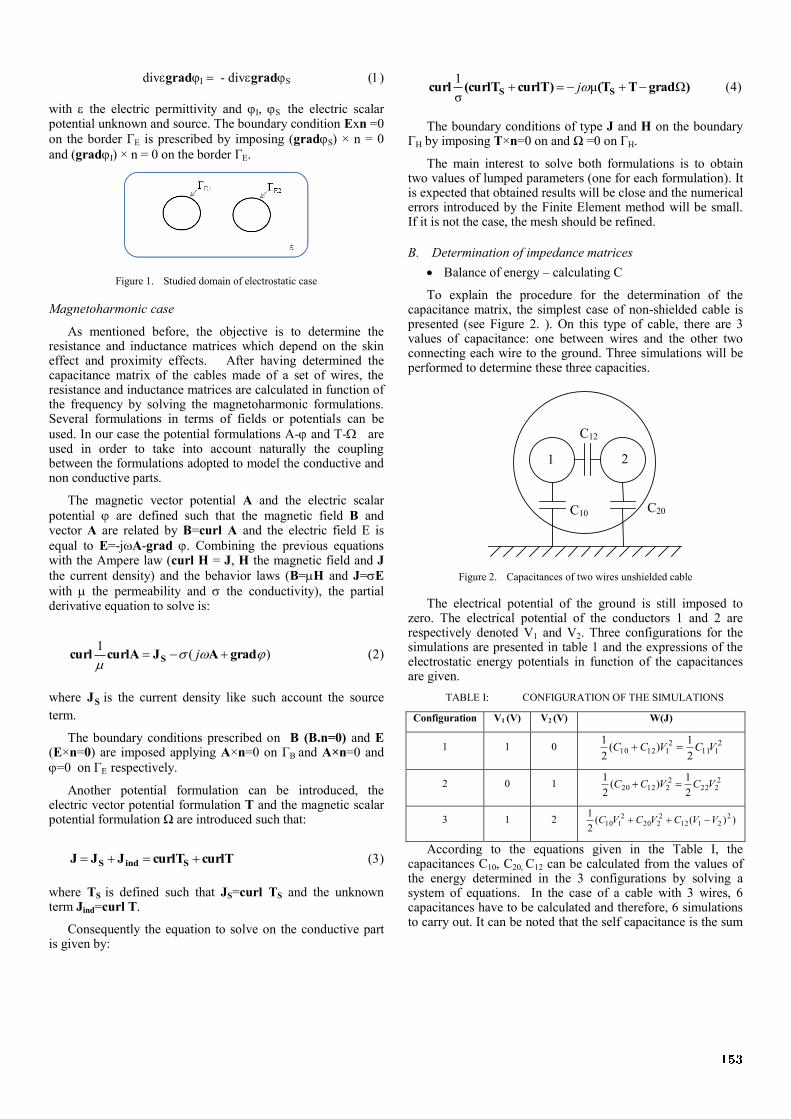
Figure 1. Studied domain of electrostatic case

Magnetoharmonic case

As mentioned before, the objective is to determine the resistance and inductance matrices which depend on the skin effect and proximity effects. After having determined the capacitance matrix of the cables made of a set of wires, the resistance and inductance matrices are calculated in function of the frequency by solving the magnetoharmonic formulations. Several formulations in terms of fields or potentials can be

used. In our case the potential formulations A- and T- are used in order to take into account naturally the coupling between the formulations adopted to model the conductive and non conductive parts.

The magnetic vector potential A and the electric scalar

potential are defined such that the magnetic field B and vector A are related by B=curl A and the electric field E is

equal to E=-jA-grad . Combining the previous equations with the Ampere law (curl H = J, H the magnetic field and J

the current density) and the behavior laws (B=H and J=E

with the permeability and the conductivity), the partial derivative equation to solve is:

)(1

gradAJcurlAcurl S j

where SJ is the current density like such account the source

term.

The boundary conditions prescribed on B (B.n=0) and E (E×n=0) are imposed applying A×n=0 on ΓB and A×n=0 and

=0 on ΓE respectively.

Another potential formulation can be introduced, the electric vector potential formulation T and the magnetic scalar potential formulation Ω are introduced such that:

curlTcurlTJJJ SindS

where TS is defined such that JS=curl TS and the unknown term Jind=curl T.

Consequently the equation to solve on the conductive part is given by:

)gradT(TcurlT)(curlTcurl SS Ωμσ

1 j

The boundary conditions of type J and H on the boundary ΓH by imposing T×n=0 on and Ω =0 on ΓH.

The main interest to solve both formulations is to obtain two values of lumped parameters (one for each formulation). It is expected that obtained results will be close and the numerical errors introduced by the Finite Element method will be small. If it is not the case, the mesh should be refined.

B. Determination of impedance matrices

Balance of energy – calculating C

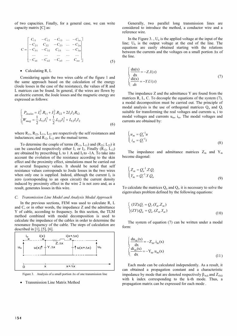
To explain the procedure for the determination of the capacitance matrix, the simplest case of non-shielded cable is presented (see Figure 2. ). On this type of cable, there are 3 values of capacitance: one between wires and the other two connecting each wire to the ground. Three simulations will be performed to determine these three capacities.

C12

C10 C20

1 2

Figure 2. Capacitances of two wires unshielded cable

The electrical potential of the ground is still imposed to zero. The electrical potential of the conductors 1 and 2 are respectively denoted V1 and V2. Three configurations for the simulations are presented in table 1 and the expressions of the electrostatic energy potentials in function of the capacitances are given.

TABLE I: CONFIGURATION OF THE SIMULATIONS

Configuration V1 (V) V2 (V) W(J)

1 1 0 2111

211210

2

1)(

2

1VCVCC

2 0 1 2222

221220

2

1)(

2

1VCVCC

3 1 2 ))((2

1 22112

2220

2110 VVCVCVC

According to the equations given in the Table I, the capacitances C10, C20, C12 can be calculated from the values of the energy determined in the 3 configurations by solving a system of equations. In the case of a cable with 3 wires, 6 capacitances have to be calculated and therefore, 6 simulations to carry out. It can be noted that the self capacitance is the sum

153

of two capacities. Finally, for a general case, we can write capacity matrix [C] as:

nnnnn

n

n

n

CCCC

CCCC

CCCC

CCCC

C

...

...............

...

...

...

321

3333231

2232221

1131211

Calculating R, L

Considering again the two wires cable of the figure 1 and the same approach based on the calculation of the energy (Joule losses in the case of the resistance), the values of R and L matrices can be found. In general, if the wires are flown by an electric current, the Joule losses and the magnetic energy are expressed as follows:

21122222

2111

1221222211

21

.2

1.

2

1

2..

IILILILW

RIIRIRIP

mag

Joules

where R11, R22, L11, L22 are respectively the self resistances and inductances; and R12, L12 are the mutual terms.

To determine the couple of terms (R11, L11) and (R22; L22) it can be canceled respectively either I1 or I2. Finally (R12, L12) are obtained by prescribing I1 to 1 A and I2 to -1A. To take into account the evolution of the resistance according to the skin effect and the proximity effect, simulations must be carried out at several frequency values. It should be noted that self resistance values corresponds to Joule losses in the two wires when only one is supplied. Indeed, although the current I2 is zero (corresponding to an open circuit) the current density induced by proximity effect in the wire 2 is not zero and, as a result, generates losses in this wire.

C. Transmission Line Model and Analysis Modal Approach

In the previous sections, FEM was used to calculate R, L and C, or in other words, the impedance Z and the admittance Y of cable, according to frequency. In this section, the TLM method combined with modal decomposition is used to calculate the impedance of the cables in order to determine the resonance frequency of the cable. The steps of calculation are described in [1], [5], [6].

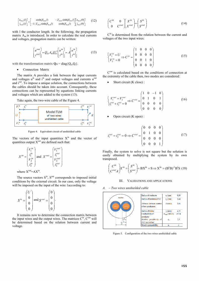
Figure 3. Analysis of a small portion ∆x of one transmission line

Transmission Line Matrix Method

Generally, two parallel long transmission lines are considered to introduce the method, a conductor wire and a reference wire.

In the Figure 3. , Ua is the applied voltage at the input of the line; Ub is the output voltage at the end of the line. The equations are easily obtained starting with the relations between the currents and the voltages on a small portion ∆x of the line.

)(.i(x)d

)(.dx

du(x)

xUYdx

xIZ

The impedance Z and the admittance Y are found from the

matrices R, L, C. To decouple the equations of the system (7),

a modal decomposition must be carried out. The principle of

modal analysis is the use of orthogonal matrices Qu and Qi

suitable for transforming the real voltages and currents u, i to

modal voltages and currents um, im. The modal voltages and

currents are obtained by:

iQi

uQu

im

um

1

1

The impedance and admittance matrices Zm and Ym

become diagonal:

uim

ium

QYQY

QZQZ

..

..1

1

(9)

To calculate the matrices Qu and Qi, it is necessary to solve the

eigenvalues problem defined by the following equations:

)..().(

)..().(

mmuu

mmii

YZQQZY

ZYQQYZ

The system of equation (7) can be written under a modal

form:

(x).uYdx

(x)di

(x).iZdx

(x)du

mmm

mmm

Each mode can be calculated independently. As a result, it

can obtained a propagation constant and a characteristic

impedance by mode that are denoted respectively m,k and Zch,k

with k index corresponding to the k-th mode. Thus, a

propagation matrix can be expressed for each mode .

154

)0(

)0(

)cosh()sinh(/1

)sinh()cosh(

)(

)(

,

,

,,

,,

,

,

km

km

kmkmch,k

kmch,kkm

km

km

i

u

llZ

lZl

li

lu

(12)

with l the conductor length. In the following, the propagation matrix Am is introduced. In order to calculate the real currents and voltages, propagation matrix can be written:

in

in

in

in

uimuiout

out

i

uA

i

uQAQ

i

u 1 (13)

with the transformation matrix Qui = diagQu,Qi.

Connection Matrix

The matrix A provides a link between the input currents

and voltages uin

and iin

and output voltages and currents uout

and iout

. To impose a unique solution, the connections between

the cables should be taken into account. Consequently, these

connections can be represented by equations linking currents

and voltages which are added to the system (13).

Take again, the two-wire cable of the Figure 4.

Figure 4. Equivalent circuit of unshielded cable

The vectors of the input quantities Xin

and the vector of

quantities output Xout

are defined such that:

in

in

in

in

in

i

V

i

V

X

2

2

1

1

and

out

out

out

out

out

i

V

i

V

X

2

2

1

1

where Xout

=AXin

.

The source vectors Sin

, Sout

corresponds to imposed initial

conditions by the external circuit. In our case, only the voltage

will be imposed on the input of the wire 1according to:

0

0

0

U

S in and

0

0

0

0

outS .

It remains now to determine the connection matrix between the input wires and the output wires. The matrices C

in, C

out will

be determined based on the relation between current and voltage.

out

in

out

in

out

in

S

S

X

X

C

C

0

0

Cin

is determined from the relation between the current and voltages of the two input wires:

0000

0100

0000

0001

02

1 in

in

in

CV

UV

Cout

is calculated based on the conditions of connection at the extremity of the cable then, two modes are considered:

Short circuit (K close) :

0000

0000

1010

0101

021

21 out

outout

outout

Cii

VV

Open circuit (K open) :

1000

0000

0010

0000

021

outoutout Cii

Finally, the system to solve is not square but the solution is easily obtained by multiplying the system by its own transposed.

SBB)B(XSBX t1-tinin

out

inin

out

in

S

SX

AC

C (18)

III. VALIDATIONS AND APPLICATIONS

A. – Two wires unshielded cable

Figure 5. Configuration of the two wires unshielded cable

155

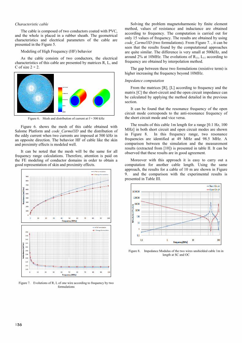
Characteristic cable

The cable is composed of two conductors coated with PVC, and the whole is placed in a rubber sheath. The geometrical characteristics and electrical parameters of the cable are presented in the Figure 5.

Modeling of High Frequency (HF) behavior

As the cable consists of two conductors, the electrical characteristics of this cable are presented by matrices R, L, and C of size 2 × 2.

Figure 6. Mesh and distribution of current at f = 500 kHz

Figure 6. shows the mesh of this cable obtained with Salome Platform and code_Carmel3D and the distribution of the eddy current when two currents are imposed at 500 kHz in an opposite direction. The behavior HF of cable like the skin and proximity effects is modeled well.

It can be noted that the mesh will be the same for all frequency range calculations. Therefore, attention is paid on the FE modeling of conductor domains in order to obtain a good representation of skin and proximity effects.

Figure 7. Evolutions of R, L of one wire according to frequency by two

formulations

Solving the problem magnetoharmonic by finite element

method, values of resistance and inductance are obtained

according to frequency. The computation is carried out for

only 15 values of frequency. The results are obtained by using

code_Carmel3D (two formulations). From Figure 7. , it can be

seen that the results found by the computational approaches

are quite similar. The difference is very small at 500kHz, and

around 2% at 10MHz. The evolutions of R11, L11 according to

frequency are obtained by interpolation method.

The gap between these two formulations (resistive term) is

higher increasing the frequency beyond 10MHz.

Impedance computation

From the matrices [R], [L] according to frequency and the

matrix [C] the short-circuit and the open circuit impedance can

be calculated by applying the method detailed in the previous

section.

It can be found that the resonance frequency of the open circuit mode corresponds to the anti-resonance frequency of the short circuit mode and vice versa.

The results of this cable 1m length for a range [0.1 Hz, 100

MHz] in both short circuit and open circuit modes are shown

in Figure 8. In this frequency range, two resonance

frequencies are identified at 49 MHz and 98.5 MHz. A

comparison between the simulation and the measurement

results (extracted from [10]) is presented in table II. It can be

observed that these results are in good agreement.

Moreover with this approach it is easy to carry out a

computation for another cable length. Using the same

approach, the results for a cable of 10 m are shown in Figure

9. and the comparison with the experimental results is

presented in Table III.

Figure 8. Impedance Modulus of the two wires unshielded cable 1m in

length at SC and OC

156

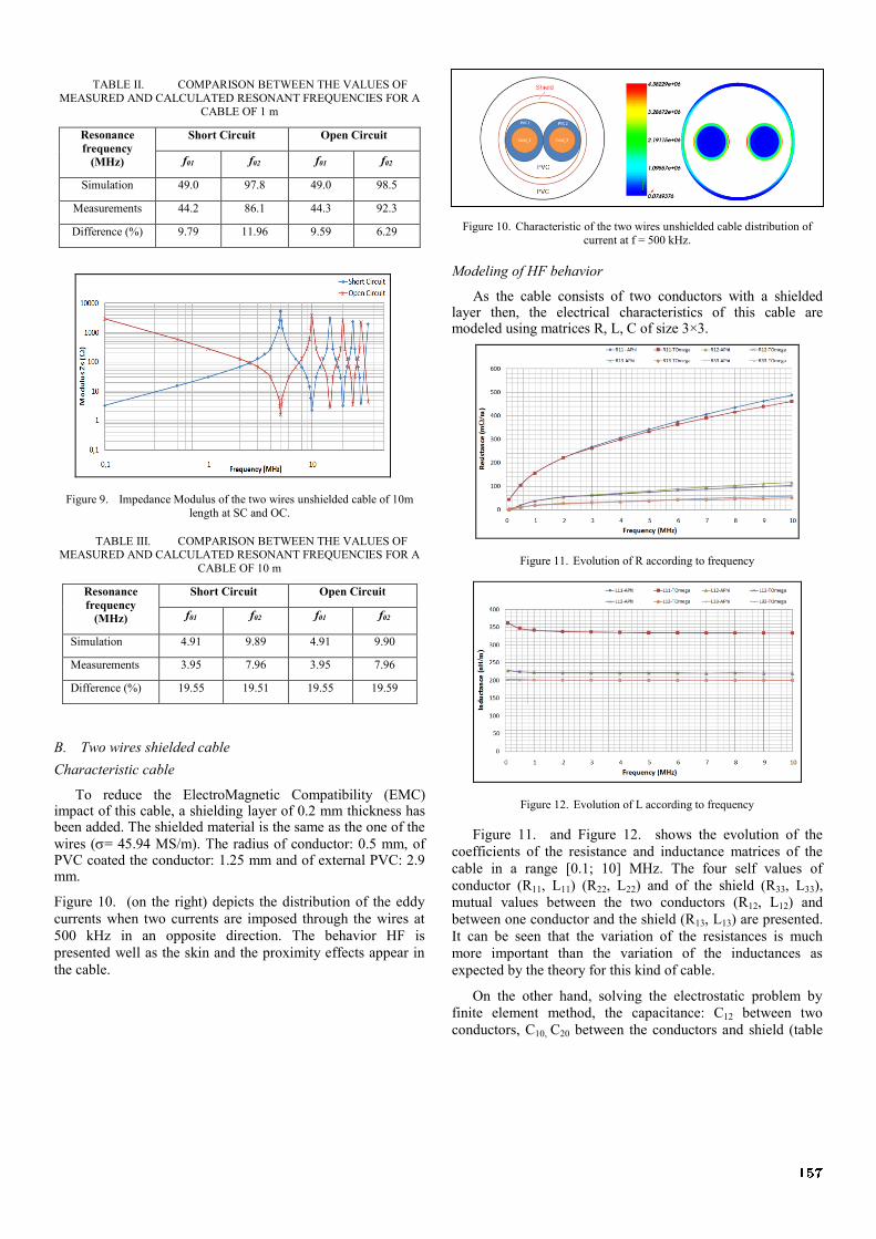
TABLE II. COMPARISON BETWEEN THE VALUES OF

MEASURED AND CALCULATED RESONANT FREQUENCIES FOR A CABLE OF 1 m

Resonance

frequency

(MHz)

Short Circuit Open Circuit

f01 f02 f01 f02

Simulation 49.0 97.8 49.0 98.5

Measurements 44.2 86.1 44.3 92.3

Difference (%) 9.79 11.96 9.59 6.29

Figure 9. Impedance Modulus of the two wires unshielded cable of 10m

length at SC and OC.

TABLE III. COMPARISON BETWEEN THE VALUES OF MEASURED AND CALCULATED RESONANT FREQUENCIES FOR A

CABLE OF 10 m

Resonance

frequency

(MHz)

Short Circuit Open Circuit

f01 f02 f01 f02

Simulation 4.91 9.89 4.91 9.90

Measurements 3.95 7.96 3.95 7.96

Difference (%) 19.55 19.51 19.55 19.59

B. Two wires shielded cable

Characteristic cable

To reduce the ElectroMagnetic Compatibility (EMC) impact of this cable, a shielding layer of 0.2 mm thickness has been added. The shielded material is the same as the one of the

wires (= 45.94 MS/m). The radius of conductor: 0.5 mm, of PVC coated the conductor: 1.25 mm and of external PVC: 2.9 mm.

Figure 10. (on the right) depicts the distribution of the eddy

currents when two currents are imposed through the wires at

500 kHz in an opposite direction. The behavior HF is

presented well as the skin and the proximity effects appear in

the cable.

Figure 10. Characteristic of the two wires unshielded cable distribution of

current at f = 500 kHz.

Modeling of HF behavior

As the cable consists of two conductors with a shielded layer then, the electrical characteristics of this cable are modeled using matrices R, L, C of size 3×3.

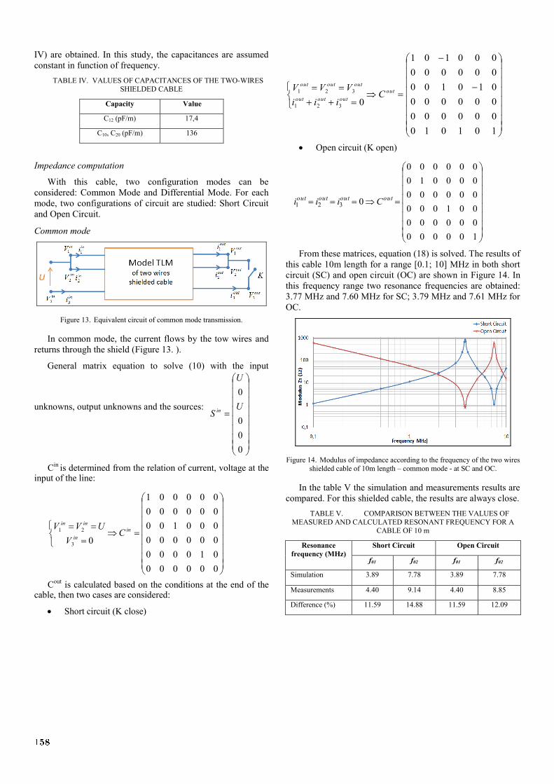
Figure 11. Evolution of R according to frequency

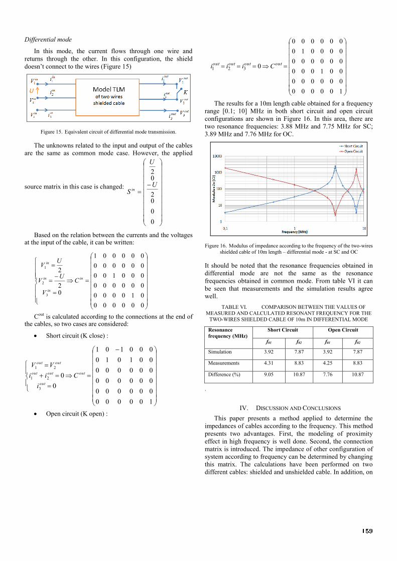
Figure 12. Evolution of L according to frequency

Figure 11. and Figure 12. shows the evolution of the

coefficients of the resistance and inductance matrices of the

cable in a range [0.1; 10] MHz. The four self values of

conductor (R11, L11) (R22, L22) and of the shield (R33, L33),

mutual values between the two conductors (R12, L12) and

between one conductor and the shield (R13, L13) are presented.

It can be seen that the variation of the resistances is much

more important than the variation of the inductances as

expected by the theory for this kind of cable.

On the other hand, solving the electrostatic problem by

finite element method, the capacitance: C12 between two

conductors, C10, C20 between the conductors and shield (table

157

IV) are obtained. In this study, the capacitances are assumed

constant in function of frequency.

TABLE IV. VALUES OF CAPACITANCES OF THE TWO-WIRES

SHIELDED CABLE

Capacity Value

C12 (pF/m) 17,4

C10, C20 (pF/m) 136

Impedance computation

With this cable, two configuration modes can be

considered: Common Mode and Differential Mode. For each

mode, two configurations of circuit are studied: Short Circuit

and Open Circuit.

Common mode

Figure 13. Equivalent circuit of common mode transmission.

In common mode, the current flows by the tow wires and

returns through the shield (Figure 13. ).

General matrix equation to solve (10) with the input

unknowns, output unknowns and the sources:

0

0

0

0

U

U

S in

Cin

is determined from the relation of current, voltage at the input of the line:

000000

010000

000000

000100

000000

000001

03

21 in

in

inin

CV

UVV

Cout

is calculated based on the conditions at the end of the cable, then two cases are considered:

Short circuit (K close)

101010

000000

000000

010100

000000

000101

0321

321 out

outoutout

outoutout

Ciii

VVV

Open circuit (K open)

100000

000000

001000

000000

000010

000000

0321outoutoutout Ciii

From these matrices, equation (18) is solved. The results of

this cable 10m length for a range [0.1; 10] MHz in both short

circuit (SC) and open circuit (OC) are shown in Figure 14. In

this frequency range two resonance frequencies are obtained:

3.77 MHz and 7.60 MHz for SC; 3.79 MHz and 7.61 MHz for

OC.

Figure 14. Modulus of impedance according to the frequency of the two wires

shielded cable of 10m length – common mode - at SC and OC.

In the table V the simulation and measurements results are

compared. For this shielded cable, the results are always close.

TABLE V. COMPARISON BETWEEN THE VALUES OF

MEASURED AND CALCULATED RESONANT FREQUENCY FOR A CABLE OF 10 m

Resonance

frequency (MHz)

Short Circuit Open Circuit

f01 f02 f01 f02

Simulation 3.89 7.78 3.89 7.78

Measurements 4.40 9.14 4.40 8.85

Difference (%) 11.59 14.88 11.59 12.09

158

Differential mode

In this mode, the current flows through one wire and

returns through the other. In this configuration, the shield

doesn’t connect to the wires (Figure 15)

Figure 15. Equivalent circuit of differential mode transmission.

The unknowns related to the input and output of the cables

are the same as common mode case. However, the applied

source matrix in this case is changed:

0

0

02

02

U

U

S in

Based on the relation between the currents and the voltages at the input of the cable, it can be written:

000000

010000

000000

000100

000000

000001

02

2

3

2

1

in

in

in

in

C

V

UV

UV

Cout

is calculated according to the connections at the end of the cables, so two cases are considered:

Short circuit (K close) :

100000

000000

000000

000000

001010

000101

0

0

3

21

21

out

out

outout

outout

C

i

ii

VV

Open circuit (K open) :

100000

000000

001000

000000

000010

000000

0321outoutoutout Ciii

The results for a 10m length cable obtained for a frequency

range [0.1; 10] MHz in both short circuit and open circuit

configurations are shown in Figure 16. In this area, there are

two resonance frequencies: 3.88 MHz and 7.75 MHz for SC;

3.89 MHz and 7.76 MHz for OC.

Figure 16. Modulus of impedance according to the frequency of the two-wires

shielded cable of 10m length – differential mode - at SC and OC

It should be noted that the resonance frequencies obtained in

differential mode are not the same as the resonance

frequencies obtained in common mode. From table VI it can

be seen that measurements and the simulation results agree

well.

TABLE VI. COMPARISON BETWEEN THE VALUES OF

MEASURED AND CALCULATED RESONANT FREQUENCY FOR THE

TWO-WIRES SHIELDED CABLE OF 10m IN DIFFERENTIAL MODE

Resonance

frequency (MHz)

Short Circuit Open Circuit

f01 f02 f01 f02

Simulation 3.92 7.87 3.92 7.87

Measurements 4.31 8.83 4.25 8.83

Difference (%) 9.05 10.87 7.76 10.87

.

IV. DISCUSSION AND CONCLUSIONS

This paper presents a method applied to determine the

impedances of cables according to the frequency. This method

presents two advantages. First, the modeling of proximity

effect in high frequency is well done. Second, the connection

matrix is introduced. The impedance of other configuration of

system according to frequency can be determined by changing

this matrix. The calculations have been performed on two

different cables: shielded and unshielded cable. In addition, on

159

the shielded cable, computations have been carried out taking

into account the two operation modes: common mode and

differential mode. Comparison of simulations with the

measurements on the value of the frequency of resonance

showed that the method gives good results. Moreover, this

method can be applied to calculate the resonant frequency for

other systems such that the three phase cable in the grid, the

four wire HVDC cable. The presented models will be

introduced in software EMTP.

ACKNOWLEDGMENT

This work is realized under the MEDEE project with

financial Assistance of European Regional Development Fund

and the region Nord-Pas-de-Calais, supported by Company

Electricity of France (EDF).

REFERENCES

[1] L. Marti, « Simulation of transients in underground cables with

frequency-dependent modal transformation matrices », IEEE

Transactions on Power Delivery, vol. 3, no. 3, pp. 1099 -1110,

july 1988.

[2] L. Haydock, R. P. Allcock, and R. N. Hampton, « Application

of a finite element technique to model an electrical power

cable », Magnetics, IEEE Transactions on, vol. 30, no. 5, pp.

3741 -3744, sept. 1994.

[3] D. da Silva, G. Fernandez, and R. A. Rivas, « Calculation of

Frequency-Dependent Parameters of Pipe-Type Cables:

Comparison of Methods », in Transmission Distribution

Conference and Exposition: Latin America, 2006. TDC ’06.

IEEE/PES, 2006, pp. 1 -6.

[4] B. Gustavsen, J. A. Martinez, and D. Durbak, « Parameter

determination for modeling system transients-Part II: Insulated

cables », IEEE Transactions on Power Delivery, vol. 20, no. 3,

pp. 2045 - 2050, july 2005.

[5] H. De Gersem, O. Henze, T. Weiland, and A. Binder,

« Transmission-line modelling of wave propagation effects in

machine windings », in Power Electronics and Motion Control

Conference, 2008. EPE-PEMC 2008. 13th, 2008, pp. 2385 -

2392.

[6] H. De Gersem and A. Muetze, « Finite-Element Supported

Transmission-Line Models for Calculating High-Frequency

Effects in Machine Windings », Magnetics, IEEE Transactions

on, vol. 48, no. 2, pp. 787 -790, feb. 2012.

[7] B. Gustavsen, A. Bruaset, J. J. Bremnes, and A. Hassel, « A

Finite-Element Approach for Calculating Electrical Parameters

of Umbilical Cables », Power Delivery, IEEE Transactions on,

vol. 24, no. 4, pp. 2375 -2384, oct. 2009.

[8] N. Bereux, « code_Carmel3D Programmer Manual version

1.5 », France, Rapport de EDF R&D, nov. 2010.

[9] N. Bereux, « code_Carmel3D Reference Manual version 1.6 »,

Rapport de EDF R&D, nov. 2010.

[10] Y. Weens, N. Idir, R. Bausiere, and J. J. Franchaud, « Modeling

and simulation of unshielded and shielded energy cables in

frequency and time domains », Magnetics, IEEE Transactions

on, vol. 42, no. 7, pp. 1876 - 1882, july 2006.

160