imperfections and self testing in prepare-and-measure
TRANSCRIPT
Imperfections and self testing inprepare-and-measure quantum key
distribution
Erik Woodhead
Laboratoire d’Information Quantique
Universite libre de Bruxelles
9 December 2014
Promoteur de these:
Serge Massar
Co-promoteur:
Stefano Pironio
Jury:
Nicolas Cerf
Pascal Kockaert
Antonio Acın
Nicolas Brunner

Abstract
Quantum key distribution (QKD) protocols are intended to allow crypto-graphic keys to be generated and distributed in a way that is provably securebased on inherent limitations, such as the no-cloning principle, imposed byquantum mechanics. This unique advantage compared with classical cryp-tography comes with an added difficulty: key bits in QKD protocols areencoded in analogue quantum states and their preparation is consequentlysubject to the usual imprecisions inevitable in any real world experiment.The negative impact of such imprecisions is illustrated for the BB84 QKDprotocol. Following this, the main part of this thesis is concerned with theincorporation of such imprecisions in security proofs of the BB84 and twosemi-device-independent protocols against the class of collective attacks. Ona technical level, by contrast with the vast majority of security proofs de-veloped since the turn of the century, in which recasting the protocol intoan equivalent entanglement-based form features heavily in the analysis, themain results obtained here are approached directly from the prepare-and-measure perspective and in particular the connection with the no-cloningtheorem and an early security proof by Fuchs et al. against the class ofindividual attacks is emphasised.
This thesis also summarises, as an appendix, a separate project which intro-duces and defines a hierarchy of polytopes intermediate between the localand no-signalling polytopes from the field of Bell nonlocality.

Contents
1 Introduction 51.1 Quantum key distribution . . . . . . . . . . . . . . . . . . . . 5
1.1.1 General background . . . . . . . . . . . . . . . . . . . 51.1.2 Contribution and outline of this thesis . . . . . . . . . 7
1.2 The BB84 protocol . . . . . . . . . . . . . . . . . . . . . . . . 101.2.1 Prepare-and-measure version . . . . . . . . . . . . . . 101.2.2 Entanglement-based version . . . . . . . . . . . . . . . 131.2.3 Correspondence . . . . . . . . . . . . . . . . . . . . . . 141.2.4 Alternatives to BB84 . . . . . . . . . . . . . . . . . . . 16
1.3 Implementation imperfections . . . . . . . . . . . . . . . . . . 171.3.1 Channel/detection noise . . . . . . . . . . . . . . . . . 171.3.2 State imprecisions . . . . . . . . . . . . . . . . . . . . 19
1.4 Security of the BB84 protocol . . . . . . . . . . . . . . . . . . 201.4.1 The no-cloning theorem . . . . . . . . . . . . . . . . . 201.4.2 Monogamy of entanglement . . . . . . . . . . . . . . . 211.4.3 Attack models . . . . . . . . . . . . . . . . . . . . . . 221.4.4 Security against individual attacks . . . . . . . . . . . 241.4.5 Security against collective attacks . . . . . . . . . . . 301.4.6 Unconditional security . . . . . . . . . . . . . . . . . . 32
1.A Comparing quantum states . . . . . . . . . . . . . . . . . . . 331.A.1 The trace norm . . . . . . . . . . . . . . . . . . . . . . 331.A.2 The trace distance . . . . . . . . . . . . . . . . . . . . 361.A.3 The fidelity . . . . . . . . . . . . . . . . . . . . . . . . 39
1.B Miscellaneous tools . . . . . . . . . . . . . . . . . . . . . . . . 401.B.1 Swap trick . . . . . . . . . . . . . . . . . . . . . . . . . 401.B.2 Schmidt decomposition . . . . . . . . . . . . . . . . . 421.B.3 von Neumann trace inequality . . . . . . . . . . . . . 42
2 Impact of device imprecisions on security 452.1 Introduction . . . . . . . . . . . . . . . . . . . . . . . . . . . . 452.2 Results . . . . . . . . . . . . . . . . . . . . . . . . . . . . . . . 48
2.2.1 Problem definition . . . . . . . . . . . . . . . . . . . . 482.2.2 Optimisation results . . . . . . . . . . . . . . . . . . . 502.2.3 Discussion . . . . . . . . . . . . . . . . . . . . . . . . . 52
1

2.3 Technical details . . . . . . . . . . . . . . . . . . . . . . . . . 532.3.1 Eve’s interaction . . . . . . . . . . . . . . . . . . . . . 532.3.2 Eve’s error rate . . . . . . . . . . . . . . . . . . . . . . 552.3.3 Inherent error rate . . . . . . . . . . . . . . . . . . . . 582.3.4 Transformation and constraints . . . . . . . . . . . . . 592.3.5 Optimisation . . . . . . . . . . . . . . . . . . . . . . . 60
2.A Partial analytic solution . . . . . . . . . . . . . . . . . . . . . 61
3 Security from cloning bounds 663.1 Introduction . . . . . . . . . . . . . . . . . . . . . . . . . . . . 67
3.1.1 Outline . . . . . . . . . . . . . . . . . . . . . . . . . . 673.1.2 Scenario and sketch of approach . . . . . . . . . . . . 68
3.2 Conditional entropy bounds . . . . . . . . . . . . . . . . . . . 703.2.1 Asymptotic key-rate bound without preprocessing . . 703.2.2 Incorporating local randomisation . . . . . . . . . . . 713.2.3 Bounding the min-entropy . . . . . . . . . . . . . . . . 73
3.3 BB84 with ideal source . . . . . . . . . . . . . . . . . . . . . . 743.4 BB84 with arbitrary source states . . . . . . . . . . . . . . . . 75
3.4.1 Derivation of fidelity bound . . . . . . . . . . . . . . . 753.4.2 Resulting key rate . . . . . . . . . . . . . . . . . . . . 763.4.3 Optimality . . . . . . . . . . . . . . . . . . . . . . . . 78
3.5 BB84 with arbitrary qubit states . . . . . . . . . . . . . . . . 813.5.1 Arbitrary measurements . . . . . . . . . . . . . . . . . 813.5.2 Qubit source and detector . . . . . . . . . . . . . . . . 86
3.A Convexity of entropy bound . . . . . . . . . . . . . . . . . . . 89
4 Semi-device-independent QKD 914.1 Introduction . . . . . . . . . . . . . . . . . . . . . . . . . . . . 914.2 Notation . . . . . . . . . . . . . . . . . . . . . . . . . . . . . . 954.3 Correlator as source characterisation . . . . . . . . . . . . . . 954.4 Correlator as channel test . . . . . . . . . . . . . . . . . . . . 98
4.4.1 Outline . . . . . . . . . . . . . . . . . . . . . . . . . . 984.4.2 Derivation of qubit y-basis bound . . . . . . . . . . . . 1004.4.3 Trace-distance bound . . . . . . . . . . . . . . . . . . 1044.4.4 Optimal collective attack . . . . . . . . . . . . . . . . 105
4.5 Comparison for depolarising channel . . . . . . . . . . . . . . 1064.A Orthogonal source states . . . . . . . . . . . . . . . . . . . . . 1074.B Convexity of asymmetric entropy bound . . . . . . . . . . . . 1094.C Characterisation of g∗ . . . . . . . . . . . . . . . . . . . . . . 110
5 Conclusion 113
A Partially deterministic polytopes 118A.1 Introduction . . . . . . . . . . . . . . . . . . . . . . . . . . . . 118
2
A.2 Preliminaries . . . . . . . . . . . . . . . . . . . . . . . . . . . 120A.2.1 Scenarios and behaviours . . . . . . . . . . . . . . . . 120A.2.2 Device-independent randomness . . . . . . . . . . . . 125A.2.3 Operations for behaviours . . . . . . . . . . . . . . . . 126
A.3 Partial determinism . . . . . . . . . . . . . . . . . . . . . . . 130A.3.1 Definition and basic properties . . . . . . . . . . . . . 130A.3.2 Local projections . . . . . . . . . . . . . . . . . . . . . 133A.3.3 The D1122(3322) polytope . . . . . . . . . . . . . . . . 136
A.A Relevant known local facets . . . . . . . . . . . . . . . . . . . 139A.A.1 Facets of the 3322 local polytope . . . . . . . . . . . . 139A.A.2 Facets of the 4322 local polytope . . . . . . . . . . . . 139
A.B Example polymake sessions . . . . . . . . . . . . . . . . . . 140
Bibliography 142
3

Foreword
This thesis reports research I was involved in during doctoral studies un-dertaken at the Laboratoire d’information quantique at the Universite librede Bruxelles during the period October 2010 – October 2014. I had theopportunity to work in a well-connected research group in quantum infor-mation theory with capable colleagues and where I was granted considerableautonomy to pursue research ideas that attracted my interest.
Doctoral research is not conducted in isolation. I would like to thank mycurrent and former colleagues and office mates of the past four years – JonSilman, Ross Duncan, Fred Ezerman, Manas Patra, Olmo Nieto Silleras,Cedric Bamps, and Damian Pitalua-Garcıa – for various combinations ofinteresting and insightful discussions, keeping me motivated to get this thesiscompleted, and sometimes encouraging me to maintain some appearance ofa social life. My co-supervisor, Stefano Pironio, followed my progress themost closely since I shared his office during the first year as a PhD student.As well as the sheer amount I learned through him simply by osmosis, I amalso indebted to him for guiding me through some of the “tools of the trade”as a beginning researcher, notably navigating the publication process andrefereeing. My thesis supervisor, Serge Massar, introduced me to the fieldof quantum information and encouraged me to start this PhD in the firstplace.
The final version of this thesis includes amendments recommended by thejury members: Nicolas Cerf, Pascal Kockaert, Nicolas Brunner, and AntonioAcın, as well as Serge Massar and Stefano Pironio.
Financially, these four years of doctoral studies were made possible by aBelgian Fonds pour la Formation a la Recherche dans l’Industrie et dansl’Agriculture (F.R.I.A.) doctoral grant.
4

Chapter 1
Introduction
1.1 Quantum key distribution
1.1.1 General background
Quantum key distribution (QKD) [1, 2] is an approach to the problem ofgenerating and distributing cryptographic keys for use in data encryption ina way that can be proved secure based on limitations inherent to quantumphysics. Since its original proposal by Charles H. Bennett and Gilles Bras-sard in 1984 [3], QKD has emerged as one of the most promising practicalapplications exploiting features of quantum physics and among the mostmature subfields of quantum information theory. QKD systems have beencommercially available since around 2004 and are, at the time of writing,offered by at least four companies [4–7].
An overview of the motivation for QKD can be found in [8]. Briefly, in thesetting considered, two spatially separated parties, traditionally called “Al-ice” and “Bob” in the literature, wish to be able to communicate privately.There are already various (classical) encryption schemes widely in use today,such as the RSA protocol commonly used to implement public key cryptog-raphy, however their security is subject to assumptions about an adver-sary’s technological and computational power and/or unproven conjecturesconcerning the difficulty of solving certain mathematical problems (e.g., inthe case of RSA, prime factorisation). There are realistic circumstances inwhich this state of affairs could be considered unsatisfactory, particularlywhere long term secrecy is a requirement, as this requires encryption thatcan reasonably be expected to remain secure against even future technology
5

of a priori unknown capability. If, for instance, a message encrypted today isto remain secret for a period of, say, fifty years, the encryption scheme mustremain practically unbreakable following any technological breakthroughsthat may occur in the next half century, which may include the develop-ment of scalable quantum computers capable of, for instance, implementingShor’s prime factorisation algorithm [9].
A resolution is to use an unconditionally secure encryption algorithm such asthe one-time pad, in which successive bits of the message to be encrypted (ifexpressed in binary) are xored with the corresponding bits of a sufficientlylong key. This, however, substitutes one problem for another: such uncon-ditionally secure algorithms require an encryption key of the same length asthe message to be encrypted, and a new encryption key must be generatedand distributed – securely – every time a new message is to be transmitted.
The problem of regular and practical distribution of secret keys is whereQKD is targeted. In its simplest description, the intent of a QKD protocol isthat a cryptographic key randomly generated by one party (“Alice”) can betransmitted to a second distant party (“Bob”) in such a way that tamperingby an adversary (usually called “Eve” in the literature) can be detected.This is achieved by Alice encoding her key bits on different nonorthogonalquantum states in such a way that any attempt to extract information byan eavesdropper will, with very high probability, disturb the transmissionof information from Alice to Bob in a visible and detectable way. Since thedistributed key should be random and in itself meaningless, failure of thistest – indicating that an eavesdropper may have learned information aboutthe key – is not fatal: Alice and Bob simply abort the protocol and mayattempt to distribute a new key at some later time.
Exploiting fundamental physical limitations implied by quantum physics,such as the measurement-disturbance tradeoff or the no-cloning principle[10, 11], the use of quantum systems promises levels of security unachiev-able with any classical system when applied to the accomplishment of cryp-tographic tasks. With these benefits, however, comes an added difficulty.Unlike classical protocols intended for execution on a digital computing de-vice and whose security is a property of a mathematically-defined algorithm,quantum protocols are specifications of physical systems that need to be im-plemented. The security of a real QKD implementation is thus dependenton the implementation closely matching the theoretical specification, and agap between theory and practice can result in the security being compro-mised. This was most strikingly demonstrated by proof-of-principle hacksof commercial QKD systems [12, 13] at the beginning of the decade, whichexploited specific properties of the components used that could allow anadversary to remotely tamper with or outright control their behaviour.
6

Implementation flaws permitting such hacks can in principle be fixed byimproving the implementation to better correspond to the theoretical spec-ification. Not all imperfections can be addressed in this way, however. AnyQKD system, as with any experiment, will always be subject to finite pre-cision of the implementation. In particular, the states prepared and thequantum measurements performed will never be exactly those required bythe theoretical specification, the channel between Alice and Bob will neverbe perfectly noiseless or lossless, and Bob’s measurement devices will neverhave perfect detection efficiency. Such imperfections must thus be expectedand accepted to some degree in any real QKD system and it is at the levelof the theoretical security analysis that they must be accounted for.
1.1.2 Contribution and outline of this thesis
The main part of this thesis is concerned with the problem of state and mea-surement imprecisions in the case of the BB84 QKD protocol, the originalprotocol proposed by Bennett and Brassard in 1984 [3]. A second, more con-ceptual motivation was the development of techniques allowing the securityof BB84-like protocols to be understood more directly from the prepare-and-measure perspective; this is by contrast with the majority of securityanalyses since around the year 2000 which recast the protocol under con-sideration into an entanglement-based form as a first step in the proof. Inparticular, the techniques that will be introduced in chapter 3 were originallyinspired by an early security proof by Fuchs et al. [14] of the prepare-and-measure BB84 protocol against a restricted class of attacks called individualattacks, and it will be shown that security proofs against the larger class ofcollective attacks can be developed in a similar style.
The remainder of this chapter consists of an introduction to the aspects ofQKD relevant to this thesis. This is not intended as a general introductionto QKD, which is already the subject of dedicated review articles [1, 2].Experimental advances (covered in [15]) and protocols other than the BB84protocol are not, for the most part, discussed here. The intent is rather tomotivate and to place the main results of this thesis in context. Section 1.2introduces and contrasts the prepare-and-measure and entanglement-basedversions of the BB84 protocol and discusses both the correspondence be-tween them and the limitations of this correspondence. Section 1.3 brieflydiscusses implementation imperfections. The emphasis is on the consider-ation of channel noise, which is standard in essentially all modern securityproofs, and source state and measurement imprecisions, which compara-tively few authors have studied. Section 1.4 is a brief introduction to thesecurity of the BB84 protocol. The section begins with the no-cloning prin-
7

ciple as it was originally formulated by Wootters and Zurek [10] and Dieks[11] in 1982, which can be considered the intuition behind the security ofthe prepare-and-measure BB84 protocol. This is contrasted with the prin-ciple of monogamy of entanglement, which can be considered the basis forthe security of the entanglement-based variant. Following this, a simplifiedderivation of the Fuchs et al. [14] security bound against individual attacksis given in the notation used later in this thesis and its connection withthe no-cloning theorem is commented on. The problem of proving securityagainst collective attacks is introduced and, finally, unconditional security(which will not be a goal in this thesis) is briefly commented on. Finally, thisintroductory chapter includes two appendices summarising a few useful defi-nitions and relations relevant to this thesis. The material should be familiarto anyone with a previous background in quantum information theory andis, for the most part, covered in textbooks and lecture notes on the subject,such as [16–18].
The main results of this thesis are collected into three chapters:
Chapter 2 first demonstrates the necessity of accounting for source stateand measurement alignment imprecisions in practical QKD securityproofs. This is achieved by demonstrating, by means of a numericaloptimisation, the existence of attacks that would allow an adversaryto learn more about the key in the presence of alignment imprecisionsthan existing security proofs where these are not accounted for wouldimply. The chapter is based on a published article, Ref. [19].
Chapter 3 introduces security proof techniques for the prepare-and-meas-ure BB84 protocol that can account for source state and measurementimprecisions against the class of collective attacks. The approach fol-lowed demonstrates that, at least for collective attacks, both knownand new security results can be derived from the prepare-and-measureperspective in a relatively straightforward way. The main result is akey rate closely resembling one derived by Marøy et al. [20] for a BB84implementation in which the source emits four arbitrary pure states(which may span a four-dimensional Hilbert space) and in which thedetectors are left uncharacterised. The key rate can be further im-proved if a preprocessing procedure called local randomisation, pro-posed in [21], is applied, and the result is shown to be tight withthe source characterisation used. As secondary results, a more spe-cific key rate is derived for arbitrary qubit source states and a furtherimproved key rate is derived if Bob’s measurements are additionallyassumed two-dimensional. The chapter is drawn from Refs. [22, 23],
Chapter 4 explores two ways in which the BB84 protocol can be modified
8

to add a degree of self certification. The protocols differ in whethereither Alice or Bob perform measurements intended to estimate aCHSH-type correlator, and their security against collective attacks isproved subject to the assumption of a two-dimensional source. Theproblem is inspired by device-independent QKD [24, 25] and a proof-of-principle prepare-and-measure semi-device-independent protocol [26].An early version of part of this work is reported in a conference pro-ceeding [27]; the remainder of this work is the subject of an articlecurrently in preparation [28] at the time of writing.
In addition, a self-contained appendix summarises work that went beyondthe theme – the security of prepare-and-measure BB84-like protocols – ofthe main part of this thesis:
Appendix A is more exploratory in nature and defines and investigates aclass of polytopes in the space of joint probability distributions inter-mediate between the local and no-signalling polytopes from the field ofBell nonlocality. This work is the subject of an article in preparation[29] at the time of writing.
The publications in question are
[19] E. Woodhead and S. Pironio, “Effects of preparation andmeasurement misalignments on the security of the Bennett-Brassard1984 quantum-key-distribution protocol”, Phys. Rev. A 87, 032315(2013).
[22] E. Woodhead, “Quantum cloning bound and application toquantum key distribution”, Phys. Rev. A 88, 012331 (2013).
[23] E. Woodhead, “Tight asymptotic key rate for the Bennett-Brassard1984 protocol with local randomization and device imprecisions”,Phys. Rev. A 90, 022306 (2014).
[27] E. Woodhead, C. C. W. Lim, and S. Pironio,“Semi-device-independent QKD Based on BB84 and a CHSH-TypeEstimation”, Theory of Quantum Computation, Communication, andCryptography, Lecture Notes in Computer Science, vol. 7582(Springer, Berlin, Heidelberg, 2013), pp. 107–115.
The articles in preparation (titles provisional) are
[28] E. Woodhead and S. Pironio, “Secrecy in prepare-and-measureCHSH games with a qubit bound”.
[29] E. Woodhead, J. Silman, and S. Pironio, “Partially deterministicpolytopes”.
9
1.2 The BB84 protocol
1.2.1 Prepare-and-measure version
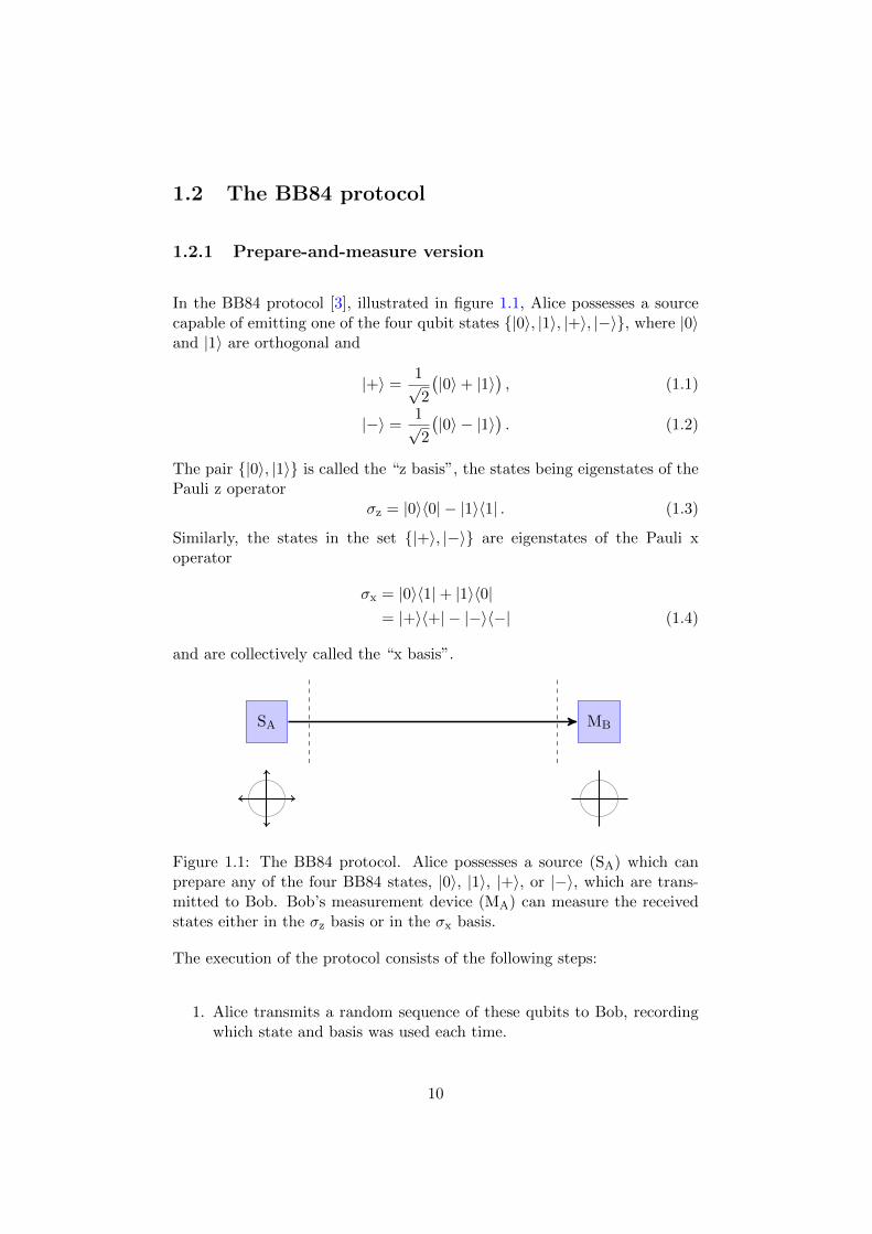
In the BB84 protocol [3], illustrated in figure 1.1, Alice possesses a sourcecapable of emitting one of the four qubit states {|0〉, |1〉, |+〉, |−〉}, where |0〉and |1〉 are orthogonal and
|+〉 =1√2
(|0〉+ |1〉
), (1.1)
|−〉 =1√2
(|0〉 − |1〉
). (1.2)
The pair {|0〉, |1〉} is called the “z basis”, the states being eigenstates of thePauli z operator
σz = |0〉〈0| − |1〉〈1| . (1.3)
Similarly, the states in the set {|+〉, |−〉} are eigenstates of the Pauli xoperator
σx = |0〉〈1|+ |1〉〈0|= |+〉〈+| − |−〉〈−| (1.4)
and are collectively called the “x basis”.
SA MB
Figure 1.1: The BB84 protocol. Alice possesses a source (SA) which canprepare any of the four BB84 states, |0〉, |1〉, |+〉, or |−〉, which are trans-mitted to Bob. Bob’s measurement device (MA) can measure the receivedstates either in the σz basis or in the σx basis.
The execution of the protocol consists of the following steps:
1. Alice transmits a random sequence of these qubits to Bob, recordingwhich state and basis was used each time.
10

2. Upon reception of each qubit, Bob randomly measures in either the σz
or σx basis, recording both the choice of basis and the result obtainedeach time.
3. Alice and Bob publicly reveal which bases they used and discard thecases where they used different bases.
4. Alice and Bob sacrifice and publicly reveal a randomly selected subsetof their results. These are used to estimate the average error rates δz
and δx in their z- and x-basis results.
At the end of this procedure, Alice and Bob each have two (random) bitstrings ZA and XA, and ZB and XB, which are their versions of the z- andx-basis keys. From the publicly revealed information in step 4, Alice and
Bob obtain an estimate of the joint prior probability distributions p(z)AB(a, b)
and p(x)AB(a, b), a, b ∈ {0, 1}, where the x-basis results + and − can be taken
to correspond to 0 and 1. The error rates are defined in terms of these by
δz = p(z)AB(0, 1) + p
(z)AB(1, 0) , (1.5)
δx = p(x)AB(0, 1) + p
(x)AB(1, 0) . (1.6)
In the cases where Bob used the same basis as Alice, their results should beperfectly correlated. In particular, if Alice chose between the two states ineach basis equiprobably, one should have
p(z)AB(0, 0) = p
(z)AB(1, 1) = p
(x)AB(0, 0) = p
(x)AB(1, 1) = 1/2 (1.7)
and δz = δx = 0.
The key feature of the BB84 protocol from which security can be guaranteedis Alice’s use of two conjugate (z and x) bases to encode the informationtransmitted to Bob. Because the four possible source states are nonorthogo-nal, no quantum measurement can perfectly distinguish between them, andan adversary attempting to gain information about the key this way willinevitably introduce errors that will reveal their presence. For example, ifan adversary attempted to learn the z-basis key bits by measuring in the σz
basis, the same operation would completely destroy any information aboutwhether Alice transmitted |+〉 or |−〉 in the cases where the x basis wasused and the adversary’s tampering would be revealed in the form of errorsbetween Alice’s and Bob’s x-basis key bits.
It is possible to prove that if the x-basis error rate δx is zero, then anadversary can have only negligible information about the z-basis key bits,and vice versa. As a first attempt at a security criterion, however, this is
11

insufficient: real world experimental implementations are never perfect and anonzero error rate is a practical inevitability. By contrast, because the intentof QKD is provable security based only on the laws of physics (as opposed tosecurity against an adversary limited by contemporary technology), for thepurpose of security analysis a nonzero error rate must always be regardedas evidence of an adversary’s presence.
Because the error rate observed in a BB84 implementation will always benonzero, then, in practice one will never be able to rule out the presence ofan adversary who may have obtained partial information about the key bits.Practically by definition, Alice and Bob will also very likely not share thesame key. This was remedied with the proposal by Bennett, Brassard, andRobert of incorporating privacy amplification [30] as well as error correctioninto the definition of the protocol:
5. If the error rates are not too high, Alice and Bob extract a (gener-ally shorter) secret key by error correction and privacy amplification.Otherwise, the protocol is aborted.
The purpose of the additional postprocessing is to allow Alice and Bobto extract a final, generally shorter, key in which the errors are corrected(Alice and Bob should share the same final key) and which is secret (aneavesdropper should have no information about the final key).
Whether and how such postprocessing can be done is a subject of researchin itself. Fortunately, sufficient criteria have been derived which reducethe problem to evaluating or bounding measures of relative randomnessor information shared between Alice, Bob, and Eve. This allows one toinvestigate the security of a QKD protocol without the need to concernoneself with the details of classical postprocessing. We will mainly use acriterion for the key rate credited to Devetak and Winter [31], which gives asimple expression for the key rate extractable by one-way1 postprocessing inthe asymptotic limit under the assumption of an individually and identicallyrepeated attack by the eavesdropper (a similar result was obtained by Kraus,Gisin, and Renner [21, 32, 33]). In the earlier part of this thesis we will alsouse an older result by Csiszar and Korner [34] from classical informationtheory, which holds for a weaker security definition.
It should be noted that there is more than one variant of the BB84 protocolthat follows the basic procedure outlined here. In the original proposal,
1This is a type of postprocessing scheme in which only one party transmits a checksumto the other. Two-way postprocessing schemes, by contrast, may involve multiple roundsof public discussion both ways.
12

for instance, Alice and Bob both select equiprobably between the z and xbases, in which case the bases will be mismatched and the results discardedhalf the time. In an alternative version proposed in [35], Alice and Bob useone basis (e.g., the z basis) the vast majority of the time for the actual keygeneration, and only occasionally use the complementary (e.g., x) basis forthe purpose of testing for the presence of an eavesdropper . In this version,the fraction of results used for key generation can be made arbitrarily closeto 1. Other variants of the BB84 protocol add additional steps to thoselisted above. It is sometimes suggested that Alice and Bob should agree onand apply a random permutation to their key bits before the postprocessingis applied, which can simplify certain security proofs [33]. A more involvedexample concerns the common case of a practical QKD system in which thekey bits are encoded on different photon (e.g., polarisation) states and anideal single-photon source is approximated by weak laser pulses attenuatedto the point that less that one photon is emitted on average in each pulse.In such an implementation there is always some probability that a givenpulse will contain two or more photons in the same state, one of which aneavesdropper could intercept without introducing any visible disturbance(the photon-number-splitting attack [36, 37]). The decoy-state technique[38, 39], which was proposed to mitigate this vulnerability, requires thatAlice select randomly between different pulse intensities during the courseof the protocol, allowing additional tests of the quantum channel.
1.2.2 Entanglement-based version
The BB84 protocol also exists in an entanglement-based version, which wasproposed by Bennett, Brassard and Mermin in 1992 [40] following a schemebased on the use of entangled states proposed by Ekert [41]. In this versionof the protocol, Alice and Bob would ideally share a number of quantumsystems each in the entangled state
|Φ+〉AB = 1√2
(|0〉A|0〉B + |1〉A|1〉B
)(1.8)
which could, for instance, be distributed by a source located midway betweenthem, and now both Alice and Bob choose randomly between performing σz
and σx measurements. Note that the entangled state also be expressed inthe x basis as
|Φ+〉AB = 1√2
(|+〉A|+〉B + |−〉A|−〉B
), (1.9)
meaning that Alice and Bob should detect perfect correlations in both thecases where they both measure in the z basis and when they both measurein the x basis. For the purpose of security analysis, the source of entangledstates is untrusted (the eavesdropper is assumed to be in control of it). In
13

this case, the eavesdropper may “attack” the protocol by preparing anddistributing a tripartite state |ψ〉ABE ∈ HA ⊗HB ⊗HE in which Eve’s partmay be entangled with Alice’s and Bob’s. The estimation of the z- andx-basis error rates is intended to detect such an attack.
1.2.3 Correspondence
There is a well known equivalence between the entanglement-based andprepare-and-measure versions of the BB84 protocol, pointed out in [40], thatis based on the following observations. First, in the prepare-and-measureversion, one way that Alice could both randomly choose and prepare eitherof the z- or x-basis states is by preparing an entangled |Φ+〉 state in herlab and measuring one part of the state in either the σz or σx bases. Thiswould project the second part of the state randomly onto one of the σz orσx eigenstates, respectively, which can then be transmitted to Bob. Second,in this implementation, Alice could just as well transmit the second part ofthe state to Bob before measuring σz or σx on her part. Third, finally, itcan only be advantageous to Eve if Eve is granted control of the source ofentangled states rather than Alice, which is recovers the entanglement-basedversion of the protocol. Specifically, this is because if Alice is in possessionof the source of Φ+ states, the best Eve could achieve with a unitary attackon the part transmitted to Bob is to transform the initial Φ+ state to atripartite state of the form
|Φ+〉AB = 1√2
(|0〉A|0〉BE + |1〉A|1〉BE
)(1.10)
for some orthogonal states |0〉BE, |1〉BE ∈ HB ⊗ HE, which is still a Φ+
state, while if Eve is in possession of the source she could substitute anytripartite state |ψ〉ABE as her attack. It follows that a security proof ofthe entanglement-based BB84 protocol would also imply the security of theprepare-and-measure version of the protocol.
To some extent, the converse may also hold. The reason for this is that anytripartite state |ψ〉ABE in which HA is two dimensional can be decomposedin the form
|ψ〉ABE =√p|0〉A|α〉BE +
√p′|1〉A|α′〉BE , (1.11)
with√p|α〉BE = (〈0|A ⊗ 1BE)|ψABE〉 and
√p′|α′〉BE = (〈1|A ⊗ 1BE)|ψABE〉,
where 1BE is the identity operator acting on HB⊗HE, such that |α〉BE and|α′〉BE are normalised and p+ p′ = 1. The same state can also be expressedin an analogous form in terms of the σx-basis states,
|ψ〉ABE =√q|+〉A|β〉BE +
√q′|−〉A|β′〉BE , (1.12)
14
with
√q|β〉 =
√p
2|α〉+
√p′
2|α′〉 , (1.13)
√q′|β′〉 =
√p
2|α〉 −
√p′
2|α′〉 . (1.14)
These relations imply constraints between the probability coefficients p, p′,q, and q′ and the inner products 〈α|α′〉 and 〈β|β′〉,
q = 12 +
√pp′Re
[〈α|α′〉
], (1.15)
q′ = 12 −
√pp′Re
[〈α|α′〉
], (1.16)
and √qq′〈β|β′〉 =
p− p′
2− i√pp′ Im
[〈α|α′〉
]. (1.17)
Note that the probability coefficients can be estimated by Alice in theentanglement-based version. In the typical case where p = p′ = q = q′ = 1/2– which Alice could verify – the constraints above simplify to
|β〉 =1√2
(|α〉+ |α′〉
), (1.18)
|β′〉 =1√2
(|α〉 − |α′〉
), (1.19)
and
Re[〈α|α′〉
]= Re
[〈β|β′〉
]= 0 , (1.20)
Im[〈α|α′〉
]= Im
[〈β|β′〉
]. (1.21)
The only difference with the situation considered in the prepare-and-measureBB84 version is that the inner products 〈α|α′〉 and 〈β|β′〉may have a nonzeroimaginary part. A security proof of the prepare-and-measure BB84 protocolmay thus also imply the security of the entanglement-based version if thenormally assumed orthogonality of the z- and x-basis source states is neverused in the security proof.
While the correspondence described above holds for the prepare-and-measureversion of the BB84 protocol as it was described in section 1.2.1, constraintsof the type described above mean that the correspondence may no longerhold for generalised versions of the protocol. In general, if Alice performsthe positive operator-valued measure (POVM) {Πa}a on her part of an ini-tial state ρABE, the part shared by Bob and Eve is projected onto a state
ρ(a)BE with probability pa given by
paρ(a)BE = TrA
[ΠaρABE
]. (1.22)
15

Using the defining property∑
a Πa = 1A for any POVM, the average overprojected states is ∑
a
paρ(a)BE =
∑a
TrA
[ΠaρABE
]= TrA[ρABE]
= ρBE , (1.23)
which is the same regardless of the measurement performed (as one shouldexpect from the no-signalling principle). Applied to the entanglement-basedversion of the BB84 protocol and in terms of the notation introduced above,this implies that the relation
p|α〉〈α|+ p′|α〉〈α| = q|β〉〈β|+ q′|β′〉〈β′| , (1.24)
called basis independence in [42], must necessarily hold between the pro-jected z- and x-basis states, even if the states are prepared by more generalmeasurements than σz and σx.
1.2.4 Alternatives to BB84
The BB84 protocol was the first QKD protocol to be proposed and remainsone of the simplest and most studied in the literature and is the protocol thatthe majority of this thesis will be concerned with. Here, we summarise a fewother notable protocols and approaches to QKD that have been proposedsince 1984.
In addition to BB84, notable “traditional” schemes include B92 [43], the six-state protocol [44, 45], and the SARG04 protocol [46]. These are similarlybased on the use of nonorthogonal source states and have various tradeoffscompared with BB84. The B92 protocol, proposed by Bennett in 1992, canbe considered the minimal QKD protocol – only two nonorthogonal sourcestates are used to encode Alice’s key bits – but has very low tolerance tonoise. The six-state protocol is identical to the BB84 protocol with the dif-ference that Alice and Bob both use the σy basis in addition to the σz andσx bases; the additional basis makes the implementation more complicatedbut permits a more thorough characterisation of the channel which slightlyimproves the six-state protocol’s tolerance to noise compared with BB84.SARG04 is intended to be more robust in implementations where the sourceimperfectly approximates a single-photon source. The protocol is based onidentical hardware to the BB84 protocol – Alice’s source ideally prepares thesame BB84 source states and Bob performs the same σx and σz measure-ments – but uses a different and more sophisticated sifting procedure than
16

BB84’s public reveal of basis choices. Other approaches, including protocolswhich use continuous degrees of freedom for encoding such as continuous-variable QKD (CV-QKD) and the coherent one-way (COW) protocol, canbe found in [2].
In the last decade, alternative proposals have appeared which aim to min-imise the assumptions needed to guarantee security, usually by introducingsome degree of self-testing as part of a protocol. The most ambitious suchproposal is so-called device-independent QKD, in which the detection ofBell-nonlocal correlations is used to certify the security and correct func-tioning of a protocol [25]; in this case, security is no longer dependent onany explicit characterisation of the devices. Intermediate approaches be-tween traditional and fully device-independent QKD also exist. These in-clude semi-device-independent QKD [26], in which the security of a prepare-and-measure scheme depends only on the assumption of a dimension boundon the devices, and measurement-device-independent QKD [47], a “reverseentanglement” scheme based on an (a priori untrusted) entangling measure-ment.
1.3 Implementation imperfections
Since its original proposal three decades ago, QKD implementations haveadvanced from lab demonstrations over less than a metre to long-distanceexperiments over ranges of a few hundred kilometres [15]. Theoretical anal-yses have progressed from the early consideration of simple intercept-resendattacks [48] to finite-key [49] unconditional security proofs based on univer-sally composable [50, 51] security definitions. The gap between theory andpractice, however, remains problematic (see [52] for a discussion publisheda few years ago). This section briefly discusses two types of imperfection –channel/detection noise and state imprecisions – that affect real QKD im-plementations. It should be stressed that, unlike the implementation flawsrevealed by the hacking attacks [12, 13] cited earlier, these are inevitable tosome degree in any real QKD system and, consequently, simply building abetter implementation will not eliminate them entirely.
1.3.1 Channel/detection noise
Historically, the first imperfection to receive explicit attention was the in-evitability of a nonzero noise rate, with the proposal of privacy amplificationmentioned in the previous section. Essentially, the idea is that if the noise
17

rate is sufficiently small, the worst case is that an adversary may have ob-tained a limited amount of information about the key to be distributed.Provided this information is limited, it may nevertheless be possible to ex-tract a shorter key in which the adversary’s information (if present) is effec-tively erased (“privacy amplification”) and relative errors between Alice’sand Bob’s versions of the key are removed (“error correction”, which willbe necessary practically by definition if we are expecting any nonzero noiserate). Consideration of noise has long been standard and expected in theo-retical work; the main purpose of a modern security proof of a given QKDprotocol is to determine whether a secret key can be extracted given that acertain noise rate has been observed (usually assuming all of the observednoise is due to an adversary’s tampering), and, if so, give an explicit lowerbound on the length of the key that can safely be extracted using knownclassical protocols for error correction and privacy amplification.
As early examples, two security results for the BB84 protocol that accountfor noise are cited here that will be relevant later in this thesis. The first isthe key rate
r = h(
12 +
√δ(1− δ)
)− h(δ) (1.25)
derived by Fuchs, Gisin, Griffiths, Niu, and Peres in 1997 [14] (hereafter the“FGGNP rate”, for convenience). In (1.25), the quantity δ is the averageerror rate observed during the execution of the protocol, h is a function calledthe binary entropy and is defined by h(x) = −x log(x)− (1− x) log(1− x),and here and throughout this thesis, we use log to denote the logarithmfunction in base 2 such that the final result is a quantity expressed in bits.The second is the Shor-Preskill key rate
r = 1− 2h(δ) (1.26)
which was first derived by Shor and Preskill in the year 2000 [53] and issimilarly expressed in terms of the average error rate δ and the binary en-tropy function h. In both cases, the key rate r (which is never greater than1 here) is the average number of key bits that can securely be extracted persignal, and in the asymptotic limit, following one-way error correction andprivacy amplification. In both cases, r = 1 if δ = 0, indicating, as one mightexpect, that the key transmitted by Alice to Bob is already secure (and nofurther postprocessing is necessary) if no errors are observed which couldbe attributed to the presence of an eavesdropper. Both key rates become 0at a certain threshold error rate (specifically δ ≈ 14.64% and δ ≈ 11.00%,for the FGGNP and Shor-Preskill rates, respectively). This can roughly bethought of as the point where an eavesdropper may have learned as muchinformation about Alice’s initial version of the key as Bob did, beyond whichthe extraction of a secret key by one-way postprocessing is no longer safe.
18

The reason we could quote two key rates for the BB84 protocol is that(1.25) and (1.26) were derived based on different underlying security defini-tions. Specifically, the authors of [14] considered a restricted class of attacks– called individual attacks in the literature – in which the eavesdropper isassumed to attack each quantum state in transit from Alice to Bob individu-ally and identically and immediately measures each state to obtain a result.The eavesdropper’s end result is their best guess of the key. The final key,following the postprocessing, is “secure” in the sense that Alice and Bobshare a uniformly random key that is completely uncorrelated from Eve’sfinal guess of the key. The Shor-Preskill rate, by contrast, was obtained asthe result of a so-called unconditional security proof, meaning that Eve’sattack is no longer assumed to be individually and identically performedon each transmitted state. More importantly, Eve is also allowed to delayher measurement indefinitely, for instance until after the postprocessing isapplied, and may even wait to find out what the key is used for before de-ciding which measurement to perform. In this case, the final key is securein the stronger sense that it is uncorrelated with any quantum informationEve might possess.
It should be noted that the gap between the threshold error rates of 11.00%and 14.64% is not fully understood. In particular, it was found in [21, 32]that the lower bound of 11% could be increased to around 12.41% if Aliceadds additional random noise to her version of the key (a preprocessingprocedure called local randomisation). Smith et al. have shown that thiscan be further increased to 12.92% with more sophisticated preprocessing[54]. In the case of two-way postprocessing, the threshold error rate is knownto be bounded between 20% and 25% [55, 56].
1.3.2 State imprecisions
A limitation of both the FGGNP and Shor-Preskill rates cited above is thatthey are derived assuming that the source states and/or measurement pro-jection operators exactly satisfy the BB84 relations described in section 1.2,i.e., in some suitable basis they exactly coincide with the σz and σx eigen-states. As a result, the cited security results are not robust in the face ofsource and/or measurement imprecisions, and the question arises as to howthey generalise in the case of source states and measurements that deviatefrom the ideal BB84 relations. This is a main theme of this thesis.
By contrast with channel noise, comparatively few theoretical security anal-yses have explicitly considered state and measurement imprecisions and itwas only earlier this year that such imprecisions were given explicit consider-
19

ation in an experimental work [57]. Security analyses of the entanglement-based BB84 protocol (or the prepare-and measure protocol with a basis-independence assumption) can be found in [42, 49, 58–60] which partiallyor fully relax the assumptions made about Alice’s and/or Bob’s measure-ments. In particular, Ref. [59] gives a generalisation of the Shor-Preskillkey rate which holds for arbitrary imprecisions on both sides in the asymp-totic limit, derived based on an entropic tradeoff relation dependent on aparameter characterising Alice’s measurement. This approach was adaptedto the case of finite statistics in [49, 60]. An early security analysis of theprepare-and-measure BB84 protocol which relaxes the basis-independenceassumption can be found in [61]. A later approach by Koashi [62], who con-sidered a source emitting arbitrary states and a perfect detector on Bob’sside, was modified by Marøy, Lydersen, and Skaar [20] to obtain a securityresult in which Alice’s source emits arbitrary states and Bob’s device is leftuncharacterised.
One of the main results of chapter 3 will be a comparatively simple deriva-tion of a key rate closely resembling the Marøy et al. key rate, complementedwith a demonstration of its optimality for the particular source charaterisa-tion used (and, technically, in the Devetak-Winter security framework thatwill be introduced in section 1.4.5).
1.4 Security of the BB84 protocol
1.4.1 The no-cloning theorem
The no-cloning theorem asserts that one cannot construct a cloning machinecapable of making multiple perfect copies of arbitrary input quantum states,i.e., there is no physical system consistent with quantum physics capable ofimplementing the operation
|ψ〉 7→ |ψ〉|ψ〉 (1.27)
that works for all input states without knowledge of the state in advance.The impossibility of perfect state cloning is obviously closely connected tothe security of QKD, in that if an eavesdropper could make perfect copiesof the quantum states in transit from Alice to Bob, they could learn theentire key by measuring their copy (if necessary, after the bases are revealed)without introducing any disturbance.
The original proof of the no-cloning theorem, by Wootters and Zurek [10]and Dieks [11], is by a counterexample based on essentially the same scenario
20

encountered in the BB84 protocol. Specifically, one considers a hypotheti-cal cloning machine designed to output perfect copies of the z-basis states,according to
|0〉A 7→ |0〉B|0〉E , (1.28)
|1〉A 7→ |1〉B|1〉E , (1.29)
in which |0〉B, |1〉B ∈ HB and |0〉E, |1〉E ∈ HE are orthonormal. Such acloner is in principle allowed in quantum physics as it satisfies unitarity,i.e., 〈0|0〉A = 〈0|0〉B〈0|0〉E = 1, 〈1|1〉A = 〈1|1〉B〈1|1〉E = 1, and 〈0|1〉A =〈0|1〉B〈0|1〉E = 0. Applying the relations
|+〉 = 1√2
(|0〉+ |1〉
), (1.30)
|−〉 = 1√2
(|0〉 − |1〉
), (1.31)
linearity of quantum operations however implies that the same cloning ma-chine necessarily transforms the x-basis states to
|+〉A 7→1√2
(|0〉B|0〉E + |1〉B|1〉E
), (1.32)
|−〉A 7→1√2
(|0〉B|0〉E − |1〉B|1〉E
), (1.33)
which differ from |+〉B|+〉E and |−〉B|−〉E, respectively. Furthermore, bothBob and Eve receive the maximally mixed density operator 1
21 = 12 |+〉〈+|+
12 |−〉〈−| regardless of whichever of |+〉A or |−〉A is used as the input. Acloner designed to output perfect duplicate copies of the two z-basis stateswould thus inevitably fail to make duplicate copies of the x-basis states, tothe point that both Bob and Eve would be completely unable to distinguishbetween the two possible input x states.
1.4.2 Monogamy of entanglement
In the entanglement-based version of the BB84 protocol, one considers theworst-case situation in which Alice, Bob, and Eve share a tripartite state|ψ〉ABE. Alice and Bob perform σz and σx measurements on their partρAB = TrE
[|ψ〉〈ψ|ABE
]of this state and estimate the z- and x-basis error
rates, whose expectation values can be expressed as
δz = 12 −
12〈σz ⊗ σz〉ρAB , (1.34)
δx = 12 −
12〈σx ⊗ σx〉ρAB , (1.35)
where in general the expectation value of an operator is given by 〈A〉ρ =Tr[Aρ]. In the ideal, noiseless situation, the security of the entanglement-based protocol can be understood in the following way. It is possible to
21

show that the only quantum state that reproduces δz = 0 and δx = 0 isthe maximally entangled pure state |Φ+〉AB =
(|0〉A|0〉B + |1〉A|1〉B
)/√
2.Essentially the only possibility in case is that Alice, Bob, and Eve shared astate of the form |Ψ〉ABE = |Φ+〉AB⊗|χ〉E, with Eve completely uncorrelatedwith Alice and Bob. This is an example of a general property of entangledstates called the monogamy of entanglement : if Alice’s and Bob’s systemsare maximally entangled with one another, which in the BB84 protocol iscertified by verifying that δz = δx = 0, then neither can be entangled at allwith a system in Eve’s possession. This rules out that Eve can learn anyinformation from her system about Alice’s or Bob’s key bits.
A simple way to see that Alice and Bob must share a Φ+ state if δz = δx = 0is to consider the sum
δz + δx = 1− 12〈σz ⊗ σz〉ρAB − 1
2〈σx ⊗ σx〉ρAB , (1.36)
which one can rearrange to
12〈W 〉ρAB = 1− δz − δx (1.37)
for the expectation value of the entanglement witness
W = σz ⊗ σz + σx ⊗ σx . (1.38)
The entanglement witness W has the two nondegenerate nonzero eigenvalues2 and −2, associated respectively with the entangled eigenstates
|Φ+〉AB =1√2
(|0〉A|0〉B + |1〉A|1〉B
), (1.39)
|Ψ−〉AB =1√2
(|0〉A|1〉B − |1〉A|0〉B
). (1.40)
Put differently, W has the spectral decomposition W = 2(|Φ+〉〈Φ+|AB −
|Ψ−〉〈Ψ−|AB
). It follows that the ideal noiseless situation δz = δx = 0, which
is equivalent to the maximal expectation value 〈W 〉ρAB = 2 for the entan-glement witness W , can only be obtained with the corresponding eigenstateρAB = |Φ+〉〈Φ+|AB.
1.4.3 Attack models
As mentioned in section 1.3.1, useful security proofs of the BB84 protocolaccount for channel noise which, from the point of view of security analysis,is treated as a side effect of tampering by an eavesdropper. Accountingfor noise, the ultimate goal of security analysis is to produce a so-called
22

“unconditional” security proof, i.e., a proof that a cryptographic key canbe extracted by error correction and privacy amplification and guaranteedsecure against any attack allowed by quantum physics that an eavesdroppermay have implemented that is compatible with some given observed errorrate. Due to the difficulty of this problem, many security analyses considerintermediate, more restricted classes of attacks in which the eavesdropperis not granted unlimited power to tamper with the channel. There aretwo such classes of attacks that we will be concerned with that appearregularly in the literature: individual and collective attacks. In both cases,the security analysis is restricted to an i.i.d. (individually and identicallydistributed) problem, in that the adversary is assumed to intercept eachstate transmitted from Alice to Bob separately and in exactly the same way,as illustrated in figure 1.2.
Alice U Bob
Eveemits
ρ
ρ′
σσ′
recvs.ρB
σ′B σB
ρ′B
recvs.ρE
σ′E σE
ρ′E
Figure 1.2: The i.i.d. unitary attack model common to both individual andcollective attacks. Alice’s source may emit any among the four BB84 statesρ = |0〉〈0|, ρ′ = |1〉〈1|, σ = |+〉〈+|, or σ′ = |−〉〈−|. Eve applies somefixed unitary operation U : H ⊇ HA → HB ⊗HE to each state individuallyemitted by Alice. Following the attack, Bob and Eve respectively receivethe corresponding state ρB, ρ′B, σB, or σ′B; and ρE, ρ′E, σE, or σ′E; dependingon which state Alice emitted.
The two attack classes, and the difference between them, can be summarisedas follows:
• In an individual attack, Eve intercepts each state emitted by Aliceseparately and applies a unitary operation with the intent of partiallycloning it. Eve then measures her intercepted part of each state, againindividually and identically, and records a classical result that willserve as her best guess of Alice’s corresponding key bit.
• In a collective attack, Eve attacks each state unitarily and individuallyand identically, as in the individual attack scenario, but no assump-tion is made on her subsequent measurement. Unlike the individualattack scenario, Eve may delay her measurement until the very end of
23

the protocol (even after error correction and privacy amplification areapplied) and may perform any joint measurement on the full collectionof intercepted states.
In an unconditional security proof, also called a security proof against a gen-eral or coherent attack, all restrictions on Eve’s allowed attack are removed.In the following subsections, we discuss individual and collective attacks,and the security of the BB84 protocol against these classes of attacks, inmore detail.
1.4.4 Security against individual attacks
In this section, we give a simplified derivation of the FGGNP rate, alreadymentioned in section 1.3.1, which was first obtained by Fuchs et al. as asecurity bound for the BB84 protocol against individual attacks. This willserve to introduce some of the notations and techniques that will be usedthoughout the remainder of this thesis.
As mentioned earlier, in the individual attack scenario, an adversary is as-sumed to attack and measure her intercepted part of each quantum statetransmitted from Alice to Bob individually and identically and before thepostprocessing is applied. For simplicity, we will consider the case whereonly the z-basis results are used to generate the key. In this case, the corre-lation between Alice’s, Bob’s, and Eve’s z-basis key bits before the postpro-cessing is described by the n-fold product of a joint probability distributionpABE(a, b, e), a, b ∈ {0, 1} which depends on the unitary attack and on Bob’sand Eve’s measurements.
The starting ingredient is a security criterion credited to Csiszar and Korner[34] stating that, in the asymptotic limit, a secret key can be extracted byone-way postprocessing from Alice to Bob at a rate which can be expressedas the difference between two conditional Shannon entropies associated withthe probability distribution pABE(a, b, e):
r = H(ZA | ZE)−H(ZA | ZB) . (1.41)
In general, the conditional Shannon entropy H(X | Y ) associated with tworandom variables X and Y is defined by
H(X | Y ) = H(XY )−H(Y ) , (1.42)
24

with the Shannon entropies H(XY ) and H(Y ) in turn defined in terms ofthe associated probability distributions by
H(XY ) = −∑xy
pXY (x, y) log(pXY (x, y)
), (1.43)
H(Y ) = −∑y
pY (y) log(pY (y)
). (1.44)
Intuitively, the conditional entropy H(ZA | ZE) is a measure of how ran-dom Alice’s record of z-basis bits is from Eve’s perspective, measuring theaverage number of key bits that can be extracted by privacy amplification.H(ZA | ZB) is similarly a measure of how random Alice’s record is fromBob’s perspective, and quantifies the key loss due to error correction. Thefinal key kA after the postprocessing, of length n ≈ rN where N is the initialnumber of z bits, is secure in the sense that the joint probability distributionis of the form
pABE(kA,kB, e) ≈(
1nδkA,kB
)pE(e) (1.45)
where
δkA,kB=
{1 : kA = kB
0 : kA 6= kB
(1.46)
is the Kronecker delta, the approximation approaching an equality in thelimit N →∞.
The problem now is to obtain a lower bound on the Csiszar-Korner rate(1.41). The conditional entropy H(ZA | ZB) presents no difficulty as itis a function of the joint probability distribution pAB(a, b) associated withAlice and Bob’s results. This can simply be estimated directly, thoughfor simplicity and anticipating that the relative errors would usually besymmetric we will replace it with h(δz), where we recall that the binaryentropy function is h(x) = −x log(x)−(1−x) log(1−x) and δz = pAB(0, 1)+pAB(1, 0) is the z-basis error rate. The less trivial problem is to derive a lowerbound for H(ZA | ZE), as this depends on the joint probability distributionpAE(a, e) which is a priori unknown. In the following we will show that theconditional entropy is lower bounded in terms of the x-basis error rate byH(ZA | ZE) ≥ h
(12 +
√δx(1− δx)
). Combining these, we will have obtained
the lower boundr ≥ h
(12 +
√δx(1− δx)
)− h(δz) (1.47)
for the Csiszar-Korner rate. The expression (1.25) given in section 1.3.1 isthe same rate in the special case where the error rates are the same, withδ = δz = δx. In this case, the FGGNP rate becomes 0 for the threshold errorrate δ = 1
2 −1
2√
2≈ 14.64%.
25

For the purpose of evaluating the conditional entropy, it will be convenientnote that it can alternatively be expressed as
H(X | Y ) = −∑x,y
pXY (x, y) log(pXY (x, y)
)+∑x
pY (y) log(pY (y)
)= −
∑x,y
pXY (x, y)[log(pXY (x, y)
)− log
(pY (y)
)]= −
∑x,y
pXY (x, y) log(pX|Y (x | y)
)=∑y
pY (y)[−∑x
pX|Y (x | y) log(pX|Y (x | y)
)]=∑y
pY (y)H(X | y) , (1.48)
where we used that pY (y) =∑
x pXY (x, y) to obtain the second line and thatpXY (x, y) = pX|Y (x | y)pY (y) to obtain the third and fourth lines. Thisestablishes that the conditional entropy H(X | Y ) is simply the averageShannon entropy of X conditioned on Y . We note that this allows for asimple derivation of an upper bound for H(ZA | ZB) in terms of δz:
H(ZA | ZB) =∑b
pB(b)H(ZA | b)
= pB(0)h(pA|B(1 | 0)
)+ pB(1)h
(pA|B(0 | 1)
)≤ h
(pB(0)pA|B(1 | 0) + pB(1)pA|B(0 | 1)
)= h(δz) , (1.49)
with the inequality on the third line following from the well known (and eas-ily verified) property of concavity of the binary entropy function. The upperbound H(ZA | ZB) ≤ h(δz) confirms that h(δz) can safely be substituted inplace of H(ZA | ZB) in the expression above for the Csiszar-Korner rate.
We now turn to the main problem of obtaining a lower bound on the con-ditional entropy H(ZA | ZE) between Alice and Eve. We begin by applying(1.48) to reexpress the entropy as
H(ZA | ZE) =∑e
pE(e)H(ZA | e)
=∑e
pE(e)h(pA|E(a | e)
)(1.50)
(for either value of a, since h(pA|E(0 | e)
)= h
(pA|E(1 | e)
)). For the purpose
of obtaining a lower bound, it will be convenient to introduce a new variableDz|e such that
H(ZA | ZE) =∑e
pE(e)h(
12 + 1
2Dz|e). (1.51)
26

The quantity Dz|e, called the “information gain” in [14], is defined by
Dz|e =∣∣pA|E(0 | e)− pA|E(1 | e)
∣∣ , (1.52)
which, using that pA|E(0 | e) + pA|E(1 | e) = 1, rearranges to
max(pA|E(0 | e), pA|E(1 | e)
)= 1
2 + 12Dz|e . (1.53)
The goal now is to determine the tradeoff between Dz|e and the x-basiserror rate δx for any unitary attack. Since a unitary operation preservesthe relative relations (inner products) between states, it is possible and willbe convenient to simply treat the source Hilbert space HA as if it were asubspace of the joint subspace shared by Bob and Eve, i.e., HA ⊂ HB⊗HE.Calling the density operators corresponding to the z-basis states ρ = |0〉〈0|and ρ′ = |1〉〈1|, the states received by Eve are the partial traces ρE = TrB[ρ]and ρ′E = TrB[ρ′]. The (conditional) probability of Eve obtaining the resulte, of corresponding POVM element Me, is then given by
pE|A(e | 0) = Tr[MeρE] or pE|A(e | 1) = Tr[Meρ′E] , (1.54)
depending on which of the z-basis states Alice sent. Assuming that Aliceselects equiprobably between them, such that pA(0) = pA(1) = 1/2, Dz|ecan be developed as
pE(e)Dz|e = |pAE(0, e)− pAE(1, e)|=∣∣1
2 Tr[MeρE]− 12 Tr[Meρ
′E]∣∣
=∣∣1
2 Tr[(1B ⊗Me)Z
]∣∣=∣∣1
2〈+|1B ⊗Me|−〉+ 12〈−|1B ⊗Me|+〉
∣∣= |Re[〈+|1B ⊗Me|−〉]| (1.55)
where Z = ρ− ρ′ = |0〉〈0| − |1〉〈1| = |+〉〈−|+ |−〉〈+|. In this way, we haveexplicitly introduced the x-basis source states into the expression for Dz|e.Representing Bob’s x-basis measurement by the POVM {F, F ′}, the x-basismeasurement can also be explicitly introduced using that 1B = F +F ′, withthe result
pE(e)Dz|e =∣∣Re[〈+|F ⊗Me|−〉] + Re[〈+|F ′ ⊗Me|−〉]
∣∣ . (1.56)
This result can be upper bounded by
pE(e)Dz|e ≤∣∣〈+|F ⊗Me|−〉
∣∣+∣∣〈+|F ′ ⊗Me|−〉
∣∣≤√〈+|F ⊗Me|+〉
√〈−|F ⊗Me|−〉
+√〈+|F ′ ⊗Me|+〉
√〈−|F ′ ⊗Me|−〉 , (1.57)
27

where the second line follows from applying the Cauchy-Schwarz inequalityto, e.g., the inner product of
√F ⊗
√Me|+〉 and
√F ⊗
√Me|−〉. (Because
the operators F , F ′, and Me are Hermitian and positive semidefinite asPOVM elements, their square roots are well defined.) Note that the resulthas the form
√a√b+√c√d; any expression of this type can be viewed as a
scalar product and, again by the Cauchy-Schwarz inequality, can be upperbounded by either
√a+ c
√b+ d or
√a+ d
√b+ c. Applying this,
pE(e)Dz|e ≤√〈+|F ⊗Me|+〉+ 〈−|F ′ ⊗Me|−〉×√〈−|F ⊗Me|−〉+ 〈+|F ′ ⊗Me|+〉
=√
Tr[(F ⊗Me)σ
]+ Tr
[(F ′ ⊗Me)σ′
]×√
Tr[(F ⊗Me)σ′
]+ Tr
[(F ′ ⊗Me)σ
], (1.58)
where we have introduced the density operators σ = |+〉〈+| and σ′ = |−〉〈−|for the x-basis states. We note that, for the four terms appearing under thesquare roots, the sum is proportional to the probability of Eve obtaining theresult e:
pE(e) = 12 Tr
[(F ⊗Me)σ
]+ 1
2 Tr[(F ′ ⊗Me)σ
]+ 1
2 Tr[(F ⊗Me)σ
′]+ 12 Tr
[(F ′ ⊗Me)σ
′] . (1.59)
We now introduce a variable δx|e defined such that
pE(e)δx|e = 12 Tr
[(F ′ ⊗Me)σ
]+ 1
2 Tr[(F ⊗Me)σ
′] , (1.60)
pE(e)(1− δx|e) = 12 Tr
[(F ⊗Me)σ
]+ 1
2 Tr[(F ′ ⊗Me)σ
′] . (1.61)
The quantity δx|e can be interpreted as the rate at which Alice and Bobwould detect errors in the x basis conditioned on Eve obtaining the result e,if Eve had measured the POVM {Me}. A property that will be importantis that they average to the x-basis error rate:∑
e
pE(e)δx|e = 12 Tr[F ′σB] + 1
2 Tr[Fσ′B] = δx . (1.62)
Applying (1.60) and (1.61) to (1.58), we find that
pE(e)Dz|e ≤√
2pE(e)δx|e
√2pE(e)(1− δx|e) , (1.63)
which simplifies to an upper bound on Dz|e that depends only on δx|e:
Dz|e ≤ 2√δx|e(1− δx|e) . (1.64)
We now return to the conditional entropy. Explicitly inserting the upperbound (1.64) forDz|e into the lower bound (1.50) for the conditional Shannonentropy,
H(ZA | ZE) ≥∑e
pE(e)h(
12 +
√δx|e(1− δx|e)
). (1.65)
28

Finally, using that the function x 7→ h(
12 +
√x(1− x)
)is convex, we obtain
the desired lower bound
H(ZA | ZE) ≥ h(
12 +
√δx(1− δx)
), (1.66)
for the conditional entropy, from which the FGGNP rate bound (1.47) abovefollows.
At this point, we have proved the security of the BB84 protocol against theclass of individual attacks under the assumption that the source states sat-isfy the ideal BB84 relations, which was used in (1.55). A worthwhile remarkis that the end result holds independently of Bob’s measurements: the condi-tional entropy H(ZA | ZB) is simply a function of the joint probability asso-ciated with Alice’s and Bob’s z-basis bits independently of the measurementperformed, while in the derivation of the lower bound on H(ZA | ZE) weused only that Bob’s x-basis measurement is an unspecified binary-outcomePOVM {F, F ′}. The authors of [14] also explicitly derived a family of op-timal unitary attacks and measurement for which the Csiszar-Korner ratecoincides with the FGGNP bound, demonstrating that the bound is in facttight.
Note that while we used the BB84 relations |±〉 = (|0〉 ± |1〉)/√
2 in orderto obtain the fourth line of (1.55), we never actually used the orthogonalityrelation 〈0|1〉 = 0, and in particular the derivation of the FGGNP rate stillholds if 〈0|1〉 is allowed a nonzero imaginary part. Following the discussionin section 1.2.3, the same rate still holds for the entanglement-based versionof the BB84 protocol.
To end this section, we remark on a connection between the derivation givenhere and the no-cloning theorem as it was outlined in section 1.4.1. First, acorollary of (1.64) that was pointed out in [14] is that∑
e
pE(e)Dz|e ≤ 2√δx(1− δx) , (1.67)
which follows because the function x 7→ 2√x(1− x) is concave. The left-
hand side can be expressed as∑e
pE(e)Dz|e =∑e
∣∣pAE(0, e)− pAE(1, e)∣∣
=∑e
12
∣∣pE|A(e | 0)− pE|A(e | 1)∣∣ . (1.68)
The second line coincides with the definition of the total variation distance(or statistical distance) between two probability distributions, which we de-note by D(pE|0, pE|1) for the probability distributions pE|0 and pE|1 of ele-ments pE|A(e | 0) and pE|A(e | 1) respectively. In terms of Eve’s marginals
29

of the z-basis states and the POVM {Me}, its quantum value is
D(pE|0, pE|1) =∑e
12
∣∣Tr[Me(ρE − ρ′E)]∣∣ . (1.69)
The maximum of (1.69) over all POVMs {Me} is a distance between thedensity operators ρE and ρ′E, which we denote by D(ρE, ρ
′E), called the trace
distance. The lowest possible x-basis error rate δx, with the minimisationtaken over all POVMs {F, F ′} Bob could perform, can likewise be expressedin terms of the trace distance between Bob’s marginals σB and σ′B of thex-basis states by δx = 1
2 −12D(σB, σ
′B). Since the tradeoff relation (1.67)
holds regardless of the measurements performed by Bob and Eve, it holdsfor the optimal measurements for which D(pE|0, pE|1) = D(ρE, ρ
′E) and δx =
12 −
12D(σB, σ
′B). Substituting these into (1.67) and rearranging, we obtain
the alternative expression
D(ρE, ρ′E)2 +D(σB, σ
′B)2 ≤ 1 (1.70)
for the tradeoff relation with the explicit appearance of the measurementoperators removed. If we define the operators Z = ρ − ρ′ and X = σ − σ′,the result can also be expressed as
14‖ZE‖ 2
1 + 14‖XB‖ 2
1 ≤ 1 (1.71)
in terms of an operator norm ‖·‖1 called the trace norm, which the tracedistance is typically defined in terms of. The counterexample used as aproof of the no-cloning theorem in section 1.4.1 is captured by the fact thatif 1
2‖XB‖1 = 1, then (1.71) implies 12‖ZE‖1 = 0, i.e., if Bob can perfectly
distinguish between the two x-basis states emitted by Alice, then Eve has noability to distinguish between the two z-basis states. Conversely, if 1
2‖ZE‖1 =1, i.e., if Eve attacks in such a way as to be able to perfectly distinguishthe z-basis states, then 1
2‖XB‖1 = 0, i.e., Bob will be unable to distinguishbetween the x states and the error rate δx will be 1/2.
1.4.5 Security against collective attacks
As mentioned in section 1.4.3, the class of collective attacks (first definedby Biham et al. [63]) is defined similarly to the class of individual attacksin that an adversary is still assumed to attack the states in transit fromAlice to Bob individually and identically. The important difference is that,in a collective attack, Eve is allowed to store her part of the quantum state(“quantum side information”) indefinitely in a quantum memory. In par-ticular, Eve may perform any collective measurement on all the quantumstates acquired via the unitary attacks and may delay her measurement until
30

after the postprocessing is applied. For this class of attacks, a lower boundon the asymptotic secret key rate extractable by one-way postprocessing isgiven by the Devetak-Winter rate [31]
r = H(ZA | E)−H(ZA | ZB) , (1.72)
The Devetak-Winter rate can be considered the analogue of the Csiszar-Korner rate which applies to the class of individual attacks. The differenceis that the conditional Shannon entropy H(ZA | ZE) which appeared inthe Csiszar-Korner rate is now replaced by the conditional von Neumannentropy H(ZA | E). This is defined by
H(ZA | E) = S(τZE)− S(τE) , (1.73)
where the von Neumann entropy is generally defined by S(ρ) = Tr[ρ log(ρ)]and (1.73) is evaluated on the classical-quantum state
τZE = pA(0)|0〉〈0|Z ⊗ ρE + pA(1)|1〉〈1|Z ⊗ ρ′E , (1.74)
where the orthogonal states |0〉Z and |1〉Z denote the state of a classical reg-ister in Alice’s possession and ρE and ρ′E are Eve’s partial traces of the z-basisstates emitted by Alice with probabilities pA(0) and pA(1) respectively, as inthe previous subsection. The state (1.74) describes the correlation betweenAlice’s record of which z-basis state was transmitted and the correspondingquantum state that Eve has managed to acquire, and replaces the joint prob-ability distribution pAE(a, e) of the previous subsection (which is no longernecessarily assumed to exist at all). The final key is secure in the strongersense that the classical-quantum state τKAKBE describing the correlationbetween Alice’s and Bob’s final keys and Eve’s quantum side informationhas the approximate form
τKAKBE ≈( ∑k∈{0,1}n
1
n|k〉〈k|KA
⊗ |k〉〈k|KB
)⊗ σE , (1.75)
with the approximation again becoming an equality in the asymptotic limit.
If the Devetak-Winter rate (1.72) is minimised for the prepare-and-measureBB84 protocol over all possible unitary attacks (or all pre-measurementtripartite states |ψ〉ABE for the entanglement-based version) for fixed errorrates δz and δx, the result is the Shor-Preskill rate
r ≥ 1− h(δx)− h(δz) . (1.76)
(The version r = 1 − 2h(δ) quoted in section 1.3.1 is a special case withδz = δx = δ.) The minimising unitary attack is, in fact, the same as theunitary part of the optimal attack that was derived by Fuchs et al. for theCsiszar-Korner rate.
31

There are several derivations of the Shor-Preskill rate as a security boundfor the BB84 protocol. The original derivation, by Shor and Preskill, wasderived based on results from the theory of entanglement purification andquantum error correction codes [53]. The first derivation as a lower boundon the Devetak-Winter or a similar rate was by Renner, Gisin, and Kraus[32]. Here, we highlight a particularly simple derivation based on a tradeoffrelation,
H(XA | B) +H(ZA | E) ≥ 1 , (1.77)
conjectured by Renes and Boileau [64] and later proved by Berta et al.[59] which holds following σx and σz measurements on the HA part of anytripartite density operator ρABE acting on HA ⊗HB ⊗HE. This allows theconditional entropy H(ZA | E) appearing in the Devetak-Winter rate tobe bounded in terms of quantities estimable by Alice and Bob working incooperation:
r = H(ZA | E)−H(ZA | ZB)
≥ 1−H(XA | B)−H(ZA | ZB)
≥ 1−H(XA | XB)−H(ZA | ZB)
≥ 1− h(δx)− h(δz) . (1.78)
Note that, in each case, the Shor-Preskill rate was derived from the entangle-ment-based perspective, i.e., the key rate was derived for the entanglement-based version of the BB84 protocol and uses the equivalence explained insection 1.2.2 in order to claim the result as a security bound for the prepare-and-measure version. In chapter 3, we will investigate how key rates canbe derived directly from the prepare-and-measure perspective, in a stylesimilar to the derivation of the FGGNP rate given in section 1.4.4, whichwill include the Shor-Preskill key rate as a special case.
1.4.6 Unconditional security
In an unconditional security proof, no assumptions are made about an ad-versary’s attack. In the asymptotic limit, the security of the BB84 protocolagainst general attacks is known to be the same as for collective attacks,i.e., the Shor-Preskill rate is still known to apply as a security bound. Itsoriginal derivation by Shor and Preskill was, in fact, in the context of anunconditional security proof. (Mayers, who is usually credited with the firstproof of unconditional security of the BB84 protocol, derived a bound onthe tolerable channel noise that was lower than the Shor-Preskill bound ofabout 11% [65]).
32

For entanglement-based QKD protocols and prepare-and-measure protocolsthat satisfy the basis-independence condition, security against collective at-tacks is known to imply unconditional security with the same key rate in theasymptotic limit. Security proofs based on the Devetak-Winter bound or asimilar result typically establish this via the exponential quantum de Finettitheorem [66] or the related postselection technique [67] for a version of theBB84 protocol in which Alice and Bob apply a random permutation to theirraw key bits. Note that such a step is necessary for security proofs basedon the Devetak-Winter rate, which was itself derived assuming an identicaland independent distribution of the underlying shared state.
The reduction to collective attacks for prepare-and-measure protocols hasnot to date received such explicit consideration. As such, the results derivedin chapters 3 and 4, which are based on the Devetak-Winter bound, aregiven as security bounds applicable to collective attacks and the question ofwhether or how they translate to unconditional security proofs will not beexplicitly addressed here.
1.A Comparing quantum states
The similarity or distinguishability of two pure quantum states |ψ〉 and |φ〉is naturally characterised by their inner product 〈φ|ψ〉. There is more thanone possible way to generalise this concept to density operators, each withdifferent uses. In this section we define and describe two ways of comparingquantum states, the trace distance and the fidelity, which are widely usedin quantum information theory and which will frequently be used in thisthesis. Both can be defined in terms of an operator norm called the tracenorm.
1.A.1 The trace norm
Definition
The trace norm of a linear operator A : H → H′, noted ‖A‖1, is defined by
‖A‖1 = Tr[|A|], (1.79)
with |A| in turn defined by |A| =√A†A. Note that A†A is positive semidef-
inite, i.e.,〈ψ|A†A|ψ〉 ≥ 0 , ∀ |ψ〉 ∈ H ; (1.80)
33

consequently its square root is well defined as the unique positive semidefi-nite operator such that
√A†A√A†A = A†A.
Alternative definitions
The trace norm admits a couple of useful equivalent alternative expressions.By the singular value decomposition theorem, there is an orthonormal ba-sis {|k〉} of H and an orthonormal basis {|k′〉} of H′ in which the operatorA takes the expression A =
∑k sk|k′〉〈k|, where the sk are real and non-
negative. In terms of this factorisation, |A| =∑
k sk|k〉〈k|, from which wefind
‖A‖1 =∑k
sk , (1.81)
i.e., the trace norm of an operator is simply the sum of its singular values.
The operator A can also be expressed in terms of |A| by A = U |A| (itspolar decomposition), where the change of basis is achieved with the unitaryU =
∑k|k′〉〈k|. Applied to (1.79), this means that there always exists a
unitary U such that‖A‖1 = Tr[UA] . (1.82)
It is possible to prove that the unitary operation above maximises the right-hand side of (1.82), from which we obtain a second expression for the tracenorm:
‖A‖1 = maxU
∣∣Tr[UA]∣∣ . (1.83)
The upper bound∣∣Tr[UA]
∣∣ ≤ ‖A‖1 is a special case of a more general in-equality. Specifically, if A and B are two linear operators (with the samedomain and codomain), then∣∣Tr[A†B]
∣∣ ≤∑k
sktk , (1.84)
where {sk} and {tk} are respectively the singular values of A and B, orderedsuch that sk ≥ sk+1 and tk ≥ tk+1.
Basic properties
It is easy to see from the various expressions given here that the trace normis indeed a matrix norm. For instance the condition ‖A‖1 = 0 ⇒ A = 0 is
34

evident from (1.82), while the property ‖A + B‖1 ≤ ‖A‖1 + ‖B‖1 followseasily from (1.83):
‖A+B‖1 = maxU
∣∣Tr[U(A+B)]∣∣
≤ maxU
(∣∣Tr[UA]∣∣+∣∣Tr[UB]
∣∣)≤ max
U
∣∣Tr[UA]∣∣+ max
U
∣∣Tr[UB]∣∣
= ‖A‖1 + ‖B‖1 . (1.85)
From (1.81), it is also clear that ‖A‖1 = ‖A†‖1.
Hermitian operators
In the case where A is Hermitian, i.e., H′ = H and A† = A, its trace norm issimply the sum of the absolute values of its eigenvalues. If A =
∑k ak|k〉〈k|
is a diagonalised expression for A, with {|k〉} forming an orthonormal basis,then |A| =
∑k|ak||k〉〈k| and
‖A‖1 =∑k
|ak| . (1.86)
The operator U appearing in (1.82) is also Hermitian in this case, and canbe obtained by U = P −Q where, for instance P and Q can be defined by
P =∑
k, ak≥0
|k〉〈k| , (1.87)
Q =∑
k, ak<0
|k〉〈k| . (1.88)
Defined this way, A = U |A|. Note that P 2 = P , Q2 = Q, PQ = QP = 0,and P + Q = 1, i.e., U is simply the difference between two orthogonalprojectors corresponding to the positive and negative eigenvalue subspacesof A. For A Hermitian, then, its trace norm can be identified by
‖A‖1 = maxU
Tr[UA] , (1.89)
where, the maximisation this time is taken over the set of Hermitian unitariesU = U †. Note that it is no longer necessary to take the absolute value, asTr[UA] is always real in this case and if U is unitary then its negation −Uis also a unitary operator. Inserting U = 2P − 1, where P is a projector,the trace norm can equivalently be obtained by
12‖A‖1 = max
PTr[PA]− 1
2 Tr[A] , (1.90)
35

with the maximisation over all projectors acting on H. Finally, we note thatthe result is unaffected if the maximisation is extended over the set of allPOVM elements:
12‖A‖1 = max
MTr[MA]− 1
2 Tr[A] , (1.91)
with M † = M and 0 ≤ M ≤ 1. To see this, it is sufficient to verifythat for any POVM element M , one can construct a projection operator Psuch that Tr[MA] ≤ Tr[PA]. Expressing M in its spectral decompositionM =
∑kmk|k〉〈k|, with 0 ≤ mk ≤ 1, the trace becomes
Tr[MA] =∑k
mk〈k|A|k〉 . (1.92)
For each value of k, 〈k|A|k〉 is either positive, in which case mk〈k|A|k〉 ≤〈k|A|k〉, or 〈k|A|k〉 is negative or zero, in which case 〈k|A|k〉 ≤ 0 by defini-tion. It follows that the sum in (1.92) is upper bounded by
∑k pk〈k|A|k〉,
with
pk =
{1 : 〈k|A|k〉 > 0
0 : 〈k|A|k〉 ≤ 0, (1.93)
and Tr[MA] ≤ Tr[PA] with P =∑
k pk|k〉〈k|.
1.A.2 The trace distance
Definition
The trace distance between two density operators ρ and σ is defined by
D(ρ, σ) = 12‖ρ− σ‖1 . (1.94)
For pure states ψ = |ψ〉〈ψ| and φ = |φ〉〈φ|, the trace distance reduces to afunction
D(ψ, φ) =√
1− |〈ψ|φ〉|2 (1.95)
of the inner product.
Basic properties of the trace distance
The trace distance satisfies the general properties of a distance measure,most of which follow from properties of the trace norm discussed above. Forinstance,
D(ρ, σ) = 0⇒ ‖ρ− σ‖1 = 0⇒ ρ− σ = 0⇒ ρ = σ . (1.96)
36

From the property ‖A+B‖1 ≤ ‖A‖1 + ‖B‖1, we obtain
D(ρ, τ) = 12‖(ρ− σ) + (σ − τ)‖1 ≤ D(ρ, σ) +D(σ, τ) (1.97)
andD(ρ, σ) ≤ 1
2‖ρ‖1 + 12‖σ‖1 = 1
2 Tr[ρ] + 12 Tr[σ] . (1.98)
The latter bound is attained if and only if ρ and σ are orthogonal. Accordingto the expression (1.94) for the trace norm of a Hermitian operator, thereexists a projection operator P for which
D(ρ, σ) = Tr[P (ρ− σ)]− 12 Tr[ρ− σ] . (1.99)
Requiring D(ρ, σ) = 12 Tr[ρ+ σ], we extract
Tr[Pρ]− Tr[Pσ] = Tr[ρ] . (1.100)
Because Tr[Pρ] ≤ ‖ρ‖1 = Tr[ρ] and Tr[Pσ] = Tr[PσP ] ≥ 0 (because PσPis positive semidefinite), (1.100) implies Tr[PρP ] = Tr[ρ] and Tr[PσP ] = 0.Similarly, for the projector Q = 1−P , Tr[QρQ] = 0 and Tr[QσQ]. Workingwith ρ and using that QρQ ≥ 0, Tr[QρQ] = 0 implies QρQ = 0, which inturn implies Q
√ρ =
√ρQ = 0. Multiplying again by
√ρ and reinserting
Q = 1− P , we obtain
PρP = ρ , (1.101)
QρQ = 0 . (1.102)
Similarly for σ,
PσP = 0 , (1.103)
QσQ = σ . (1.104)
ρ and σ are thus orthogonal in the sense that their support is on orthogonalsubspaces.
If ρ and σ are properly normalised, i.e., if Tr[ρ] = Tr[σ] = 1, then the factorof 1/2 in (1.94) guarantees D(ρ, σ) ≤ 1, again with equality if and only if ρand σ are orthogonal.
Finally, a useful property of the trace distance is that it can only decreasefollowing partial tracing, i.e., if ρA = Tr[ρAB] and σA = TrB[σAB], then
D(ρA, σA) ≤ D(ρAB, σAB) . (1.105)
37
This is easily seen by expressing the trace distance as a maximisation overprojection operators:
D(ρA, σA) = maxPA
Tr[PA(ρA − σA)
]= max
PA
Tr[(PA ⊗ 1B)(ρAB − σAB)
]≤ max
PAB
Tr[PAB(ρAB − σAB)
]= D(ρAB, σAB) . (1.106)
Relevance to state discrimination
The trace distance has a well known operational significance in the context ofstate discrimination. Specifically, suppose one wishes to distinguish betweentwo density operators ρ and σ, drawn with equal probability, i.e., p(ρ) =p(σ) = 1/2, with a binary outcome measurement described by a POVM{M,N}. IfM is intended to detect the state ρ andN the state σ, the averageprobability of correctly guessing the state (called the “guessing probability”)is given by
Pguess = p(ρ,M) + p(σ,N)
= 12p(M | ρ) + 1
2p(N | σ)
= 12 Tr[Mρ] + 1
2 Tr[Nσ]
= 12 + 1
2 Tr[M(ρ− σ)
], (1.107)
where we inserted N = 1−M to obtain the final line. From the expression(1.91) for the trace norm, and noting that Tr[ρ−σ] = 0, we obtain a versionof the Helstrom bound [68]:
Pguess ≤ 12 + 1
2D(ρ, σ) . (1.108)
The lower bound Pguess ≥ 12 −
12D(ρ, σ) can be obtained in a similar way.
In QKD, it is more conventional to express security bounds in terms of theerror rate δ, i.e., the average probability of incorrectly identifying the state.In anticipation of this, we note that the Helstrom bound can equivalentlybe given for the error rate:
12 −
12D(ρ, σ) ≤ δ ≤ 1
2 + 12D(ρ, σ) , (1.109)
which can be obtained by essentially the same derivation as the Helstrombound for Pguess given above, or simply by using that δ = 1 − Pguess. Notethat the lower and upper bounds in (1.109) can be rearranged to give
D(ρ, σ) ≥ |1− 2δ| . (1.110)
38

Expressed this way, the average error rate provides a lower bound on thetrace distance between ρ and σ.
If the states ρ and σ are drawn with prior probabilities p(ρ) = p and p(σ) =q = 1− p, the Helstrom bound generalises to
12 −
12‖pρ− qσ‖1 ≤ Pguess ≤ 1
2 + 12‖pρ− qσ‖1 (1.111)
and‖pρ− qσ‖1 ≥ |1− 2Pguess| . (1.112)
1.A.3 The fidelity
Definition
The fidelity is a comparison measure between density operators that wasintroduced by Josza [69]. Unlike the trace distance, it does not have anobvious operational significance, however it will prove useful as an interme-diate quantity in certain derivations. In this thesis, for two density operatorsρ and σ we will take the fidelity to be defined by
F (ρ, σ) = ‖√ρ√σ‖1 . (1.113)
It should be noted that it is sometimes the square of (1.113) that is called the“fidelity” in the literature. By contrast with the trace distance, the fidelity isa measure of “closeness” of two states in the sense that F (ρ, σ) = 1 if ρ = σand F (ρ, σ) = 0 if ρ and σ are orthogonal. If ψ = |ψ〉〈ψ| and φ = |φ〉〈φ| arepure states, the fidelity reduces to the inner product F (ψ, φ) = |〈ψ|φ〉|.
Uhlmann’s theorem
An important alternative definition of the fidelity is given by Uhlmann’stheorem, which states that
F (ρ, σ) = maxψ,φ
∣∣〈ψ|φ〉∣∣ , (1.114)
with the maximisation taken over all purifications |ψ〉 and |φ〉 of the densityoperators ρ and σ, i.e., subject to the constraints ρA = TrB
[|ψ〉〈ψ|AB
]and
σA = TrB
[|φ〉〈φ|AB
]if ρ and σ are taken to act on the Hilbert space HA
and |ψ〉 and |φ〉 are vectors in an extended Hilbert space HA ⊗HB.
39

Uhlmann’s theorem can be proved in the following way. We express ρand σ in terms of their spectral decompositions ρ =
∑k pk|αk〉〈αk| and
σ =∑
j qj |βk〉〈βk|, which we use to define the (unnormalised) state |Φ+〉 =∑k|αk〉|k〉 for any arbitrary basis {|k〉} of an auxiliary Hilbert space and
the unitary V =∑
k|βk〉〈αk|. In terms of these, note that
|ψ〉 =√ρ⊗ 1|Φ+〉 , (1.115)
|φ〉 = (√σV )⊗ 1|Φ+〉 , (1.116)
are purifications of ρ and σ, respectively, which expand to their Schmidtdecompositions. In terms of these, for the fidelity we obtain
F (ρ, σ) = maxU
∣∣Tr[U√ρ√σ]∣∣ (1.117)
= maxU
∣∣Tr[U√ρ√σV]∣∣ (1.118)
= maxU
∣∣〈Φ+|(√ρ√σV )⊗ Uᵀ|Φ+〉
∣∣ (1.119)
= maxU
∣∣〈ψ|1⊗ U |φ〉∣∣ . (1.120)
Since 1 ⊗ U |φ〉 is still a purification of σ for any unitary U , and all pu-rifications of a density operator are related by unitaries on the auxiliary(purifying) Hilbert space, the final line is simply a maximisation over allpurifications of ρ and σ.
Relation to the trace distance
Uhlmann’s theorem can be used to derive an upper bound [70],
D(ρ, σ) ≤√
1− F (ρ, σ)2 , (1.121)
on the trace distance in terms of the fidelity. To see this, we take |ψ〉 and|φ〉 to be purifications of ρ and σ such that F (ρ, σ) = |〈ψ|φ〉|. Using thatthe trace distance can only decrease as a result of partial tracing,
D(ρ, σ) ≤ D(ψ, φ) =√
1− |〈ψ|φ〉|2 =√
1− F (ρ, σ)2 . (1.122)
1.B Miscellaneous tools
1.B.1 Swap trick
Given a maximally entangled bipartite state
|Φ+〉 =1√N
N∑k=1
|k〉A|k〉B ∈ HA ⊗HB (1.123)
40

and any operator A acting on HA, a useful identity is
A⊗ 1|Φ+〉 = 1⊗Aᵀ|Φ+〉 . (1.124)
The transpose in (1.124) is taken relative to the basis in which the |Φ+〉state is defined. Specifically, if the operator A has matrix elements 〈j|A|k〉,then Aᵀ is taken to be the operator such that 〈j|Aᵀ|k〉 = 〈k|A|j〉. The proofproceeds by inserting the identity 1A =
∑j |j〉〈j|A and rearranging terms:
√NA⊗ 1|Φ+〉 =
(∑j
|j〉〈j|A)A⊗ 1
(∑k
|k〉A|k〉B)
=∑jk
|j〉A〈j|A|k〉A|k〉B
=∑jk
|j〉A|k〉B〈k|Aᵀ|j〉B
=∑j
1⊗Aᵀ|j〉A|j〉B . (1.125)
A related identity, for the trace of the product of two operators, is
Tr[AB] = N〈Φ+|A⊗Bᵀ|Φ+〉 , (1.126)
which can be obtained by a similar derivation as (1.124):
Tr[AB] =∑k
〈k|AB|k〉
=∑jk
〈k|A|j〉〈j|B|k〉
=∑jk
〈k|A|j〉A〈k|Bᵀ|j〉B
=(∑
k
〈k|A〈k|B)A⊗Bᵀ
(∑j
|j〉A|j〉B)
= N〈Φ+|A⊗Bᵀ|Φ+〉 . (1.127)
The relations above can be useful in problems involving a maximisation overa given set of operators, especially where the set as a whole is invariant undertransposition. For instance, the transpose of a Hermitian operator is stillHermitian and the transpose of a unitary operator is still unitary.
41

1.B.2 Schmidt decomposition
It is possible to show that any bipartite pure state |ψ〉 ∈ HA ⊗HB admitsan expression of the form
|ψ〉 =∑k
λk|k〉A|k〉B , (1.128)
in which {|k〉A} and {|k〉B} are, respectively, orthonormal bases of HA andHB and all the coefficients λk are real and nonnegative.
The Schmidt decomposition can be arrived at in the following way: first,we find the marginal density operator ρ = TrB
[|ψ〉〈ψ|
], which we express in
terms of its spectral decomposition ρ =∑
k pk|k〉〈k|A. We then expand |ψ〉in the basis {|k〉A} composed of its eigenstates, obtaining
|ψ〉 =(∑
k
|k〉〈k|A ⊗ 1B
)|ψ〉 =
∑k
|k〉A|k〉B , (1.129)
where |k〉B =(〈k|A ⊗ 1B
)|ψ〉. Finally evaluating ρ again,
ρ =∑jk
|j〉〈k|A〈k|j〉B , (1.130)
which only recovers the spectral decomposition of ρ if 〈j|k〉B = pkδjk. TheSchmidt decomposition is obtained by substituting |k〉B =
√pk|k〉B and√
pk = λk.
A corollary of the derivation of the Schmidt decomposition given here isthat all purifications of a density operator ρ, i.e., pure states |ψ〉 ∈ HA⊗HB
such that ρ = TrB
[|ψ〉〈ψ|
], differ only by unitary operations acting on the
auxiliary Hilbert space. if |ψ〉 and |ψ′〉 are two purifications of ρ, accordingto the derivation given above they can be expressed in terms of their Schmidtdecompositions |ψ〉 =
∑k
√pk|k〉A|k〉B and |ψ′〉 =
∑k
√pk|k〉A|k′〉B for the
same set {|k〉A} of eigenstates of ρ. |ψ〉 and |ψ′〉 are then related by |ψ′〉 =1⊗U |ψ〉 for the unitary U =
∑k|k′〉〈k|B. Conversely, if |ψ〉 is a purification
of ρ and U a unitary operation, then |ψ′〉 = 1⊗ U |ψ〉 is still a purification:TrB
[|ψ′〉〈ψ′|
]= TrB
[U |ψ〉〈ψ|U †
]= TrB
[|ψ〉〈ψ|
]= ρ.
1.B.3 von Neumann trace inequality
For A, B Hermitian, the trace of their product is upper bounded by
Tr[AB] ≤∑k
akbk , (1.131)
42
in which ak and bk are the eigenvalues of A and B respectively, listedin decreasing order such that ak ≥ ak+1 and bk ≥ bk+1. This can beobtained by substituting spectral decompositions A =
∑j aj |αj〉〈αj | and
B =∑
k bk|βk〉〈βk| for A and B:
Tr[AB] =∑jk
ajbk∣∣〈αj |βk〉∣∣2
=∑jk
ajSjkbk
= aᵀSb , (1.132)
where we have introduced the matrix S of elements Sij =∣∣〈αj |βk〉∣∣2, and a
and b are the column matrices of elements aj and bk, respectively. Note that∑j Sjk =
∑k Sjk = 1 and Sjk ≥ 0, meaning that S is a doubly stochastic
matrix and thus (by the Birkhoff-von Neumann theorem) can be expressedas a convex sum of permutation matrices
S =∑σ
pσΠσ , (1.133)
with pσ ≥ 0,∑
σ pσ = 1, and the permutation matrix Πσ is of elements
Π(σ)jk = δj,σ(k). Consequently,
Tr[AB] =∑σ
pσaᵀΠσb
≤ maxσ
aᵀΠσb
= maxσ
∑jk
δj,σ(k)ajbk
= maxσ
∑k
aσ(k)bk
=∑k
akbk . (1.134)
Because the spectrum of a Hermitian operator is a unitary invariant (in thesense thatA and UAU † have the same eigenvalues), an alternative expressionis
maxU
Tr[AUBU †] =∑k
akbk . (1.135)
The equality Tr[AUBU †] =∑
k akbk is clearly attainable with U =∑
k|αk〉〈βk|,for which UBU † is diagonal in the same basis as A.
More generally for, operators A,B : H → H′, a similar inequality creditedto John von Neumann [71] holds in terms of their singular values {sj} and
43

{tk}: ∣∣Tr[A†B]∣∣ ≤∑
k
sktk , (1.136)
with the singular values similarly listed in decreasing order. The analogueof (1.135) is
maxU,V
∣∣Tr[A†UBV †]∣∣ =
∑k
sktk , (1.137)
with the maximisation taken over unitaries U : H → H and V : H′ → H′.
A simple corollary of the von Neumann trace inequality is that
|Tr[AB]| ≤ ‖A‖1‖B‖∞ , (1.138)
with the ∞-norm defined by ‖B‖∞ = limp→∞Tr[|B|p
]1/p, i.e., the maxi-
mum singular value of B.
44

Chapter 2
Impact of deviceimprecisions on security
The main purpose of this chapter is to demonstrate the negative impact ofsource and measurement imprecisions on the security of the BB84 protocol.This is achieved by numerically minimising the key rate against an adversaryrestricted to individual attacks, for which necessary and sufficient conditionsare known, which is shown to decrease in cases where Alice’s and Bob’s basesare allowed to differ from σz and σx. With the exception of section 2.A, thework presented here was earlier reported in [19], on which this chapter is based.The project itself originated from a loose collaboration with the authors of[72, 73], who similarly explored the effect of imperfections in the alignmentof measurement bases on the characterisation of quantum resources throughquantum state tomography and entanglement witnesses. In the context of thisthesis, this chapter motivates and establishes the necessity of the work detailedin chapters 3 and 4.
While working on the project, it was initially attempted to derive the the key rateanalytically. An early partial result in this direction is included as appendix 2.Aat the end of this chapter, as it may be of interest in itself.
2.1 Introduction
In the BB84 protocol, Alice emits one of two states |α〉 or |α′〉, which wecollectively call the “z basis”, or one of the two states |β〉 or |β′〉, which we
45

collectively call the “x basis”. The other party (“Bob”) then randomly mea-sures each qubit he receives in one of two bases {|A〉, |A′〉} or {|B〉, |B′〉}. Asdiscussed in section 1.2.1, in its ideal formulation, the states {|α〉, |α′〉} and{|β〉, |β′〉} prepared by Alice are supposed to constitute orthogonal bases,i.e., the states should satisfy the orthogonality relations
〈α|α′〉 = 〈β|β′〉 = 0 . (2.1)
Furthermore, the two bases on Alice’s and on Bob’s sides are supposed tobe mutually unbiased, i.e., they should differ exactly by an angle of π/2, orsatisfy the relations1
|β〉 = 1√2
[|α〉+ |α′〉
], (2.2a)
|β′〉 = 1√2
[|α〉 − |α′〉
], (2.2b)
and
|B〉 = 1√2
[|A〉+ |A′〉
], (2.3a)
|B′〉 = 1√2
[|A〉 − |A′〉
]. (2.3b)
While existing security proofs for BB84 routinely account for channel noise,most security analyses take for granted that the source states and measure-ment precisely satisfy the conditions (2.1), (2.2), and (2.3). As was stressedin the introduction, imprecisions are inevitable in a realistic implementationof the protocol. For instance, the measurement of a polarisation qubit maynot be more precise than, say, 2◦ or 4◦ (on the Bloch sphere) due to the in-trinsic uncertainty of the polarisation rotator used. Such imperfections mayallow an eavesdropper to gain more information about the shared key thanexisting security proofs would imply. While some theoretical security anal-yses have relaxed these assumptions, such as those cited in section 1.3.2,they were generally not applied to experimental QKD demonstrations atthe time the work outlined here was originally undertaken [74] and it is onlyvery recently that such imprecisions were given explicit consideration in anexperimental project [57].
The main purpose of this chapter is to illustrate the negative impact of stateand measurement alignment imprecisions on the performance of a QKDprotocol, specifically in the case of the BB84 protocol with one-way post-processing. Instead of deriving a new security proof, the aim is rather to
1In addition, in the ideal formulation, the bases on Alice’s and Bob’s sides are usuallytaken to be perfectly aligned, i.e., |α〉 = |A〉, |α′〉 = |A′〉, |β〉 = |B〉, and |β′〉 = |B′〉.This is a non issue from the point of view of security analysis, however, as any relativemisalignment between Alice’s and Bob’s bases can be absorbed into the adversary’s unitaryattack.
46

demonstrate an explicit advantage gained by an eavesdropper. For this pur-pose, the analysis is restricted to individual attacks for which necessary andsufficient conditions for security are known, for which we optimise over allpossible unitary individual attacks in the presence of imperfections.
Note that this approach contrasts with existing security proofs which ac-count for device imprecisions, such as those mentioned in section 1.3.2. Suchsecurity proofs derive lower bounds on the secret key rate, i.e., they boundthe security “from below” (ruling out possible successful attacks by an eaves-dropper below a certain threshold) and is not a priori clear whether and towhat extent any reduction in the key rate is genuine and not an artefact ofa suboptimal security proof or overly demanding security definition. Sincethe key rates given in this chapter were obtained by minimising over anadversary’s possible individual attacks, i.e., security was bounded “fromabove”, they represent an upper bound on security in that nonideal BB84implementations of the type considered here are proved insecure beyonda certain threshold. Any reduction in the key rate below known securitybounds proved for an ideal BB84 implementation thus indicates a genuineadvantage that could be exploited by an eavesdropper.
For simplicity, the analysis is restricted to the case where the states emittedby Alice still form two orthonormal bases as in (2.1). (Any deviation from(2.1) can only reinforce the effects of imperfections that will be illustratehere.) We suppose, however, that Alice’s preparation and Bob’s measure-ment bases are not exactly mutually unbiased, but that they differ by anglesϕA and ϕB, respectively, different from π/2. That is, we suppose instead of(2.2) and (2.3) that
|β〉 = cos(ϕA
2
)|α〉+ sin
(ϕA2
)|α′〉 , (2.4a)
|β′〉 = cos(ϕA
2
)|α′〉 − sin
(ϕA2
)|α〉 , (2.4b)
and
|B〉 = cos(ϕB
2
)|α〉+ sin
(ϕB2
)|α′〉 , (2.5a)
|B′〉 = cos(ϕB
2
)|α′〉 − sin
(ϕB2
)|α〉 . (2.5b)
It is clear that such errors will in general reduce the security of BB84.For example, in the extreme case where the two bases accidentally coincide(ϕA, ϕB = 0), an eavesdropper could perfectly clone the states sent by Alicewithout revealing her presence. In this chapter, we will demonstrate moregenerally a reduction in the extractable secret key rate of the BB84 protocolagainst individual attacks, for a given error rate, when ϕA, ϕB 6= π/2.
Though the reduction in the key rate that we observe is small for deviationsfrom the ideal situation expected in realistic implementations, the results,
47

given in section 2.2, nevertheless show that Alice and Bob can erroneouslyconclude that they have established a secure key if the inevitable experimen-tal errors in the alignment of the bases are not taken into account. Technicaldetails concerning the derivation of the results presented in section 2.2 aredeferred to section 2.3.
2.2 Results
2.2.1 Problem definition
As explained in section 1.4.4, in the case of one-way communication fromAlice to Bob, the asymptotic key rate secure against individual attacks isgiven by the Csiszar-Korner bound, which we express as
r = H(KA | KE)−H(KA | KB) (2.6)
in terms of the conditional Shannon entropies H(KA | KE) and H(KA | KE)between Alice and Eve and between Alice and Bob, respectively. We willmainly consider the original version of the BB84 protocol in which Aliceand Bob both use the z and x bases equiprobably and the sifted results fromboth bases are used to generate the final key. In order to accommodate thisin (2.6) we formally treat the choice of basis (which is public knowledge) aspart of the key, i.e. KA = (A,U) and KB = (B, V ). In this case, for instancefor the conditional entropy between Alice and Bob,
H(KA | KB) = H(AU | BV )
= H(ABUV )−H(BV )
= H(A | B;UV ) +H(BUV )−H(BV ) . (2.7)
Since we are considering only the results where Alice and Bob chose thesame basis, for our purposes V = U , in which case (2.7) simplifies to
H(KA | KB) = H(A | B;U)
=∑u
pU (u)H(A | B;U = u)
= pzH(ZA | ZB) + pxH(XA | XB) , (2.8)
where pz and px (pz + px = 1) are the probabilities that Alice and Bob usethe z and x bases, respectively. A similar result holds for H(KA | KE). Theresult, as one might expect, is that the key rate is simply the average of theCsiszar-Korner rates in each basis:
r = (rz + rx)/2 , (2.9)
48

where
rz = H(ZA | ZE)−H(ZA | ZB) , (2.10)
rx = H(XA | XE)−H(XA | XB) , (2.11)
and we inserted explicitly pz = px = 1/2.
Recall that, in the case of individual attacks, Eve performs the same unitaryattack and measures her intercepted part of each state individually. Follow-ing Fuchs et al. [14], we also allow Eve to possess a quantum memory and todelay her measurements on the states in her possession until after the basesare revealed (but not until after the postprocessing). In this case, as wasmentioned in 1.4.4, the asymptotic key rate under conditions (2.1), (2.2),(2.3) is given in terms of δ by
r = h(
12 +
√δ(1− δ)
)− h(δ) , (2.12)
where h = −x log(x) − (1 − x) log(1 − x) is the binary entropy functionexpressed in bits.
Our task is to minimise the expression (2.6) for a given average error rateδ using the preparation and measurement bases defined by (2.4) and (2.5)rather than the ideal ones. To simplify the analysis we will assume that theerrors observed between Alice and Bob are symmetric, i.e.,
p(z)AB(0, 1) = p
(z)AB(1, 0) = p
(x)AB(0, 1) = p
(x)AB(1, 0) , (2.13)
in which case the error rates in the z and x bases, δz and δx, are the same.Given our assumptions about the symmetries in the errors observed by Aliceand Bob, H(KA | KB) is a simple function of δ:
H(KA | KB) = H(ZA | ZB) = H(XA | XB) = h(δ) . (2.14)
In general there need not be such symmetries in the joint probabilities
p(u)AE(a, e) shared between Alice and Eve, and H(KA | KE) is accordingly
more complicated. In each basis it will be convenient to parameterise thesequantities in terms of an error ∆u dependent on the basis u ∈ {z, x} analo-gous to the error rate, and an offset υu:
p(u)AE(0, 0) = 1
2(1−∆u − υu) , (2.15a)
p(u)AE(0, 1) = 1
2(∆u + υu) , (2.15b)
p(u)AE(1, 0) = 1
2(∆u − υu) , (2.15c)
p(u)AE(1, 1) = 1
2(1−∆u + υu) . (2.15d)
49

The inverse relations are ∆u = p(u)AE(0, 1) + p
(u)AE(1, 0) and υu = p
(u)AE(0, 1) −
p(u)AE(1, 0). The conditional entropy between Alice and Eve is given by
H(KA | KE) = 12
(H(ZA | ZE) +H(XA | XE)
), (2.16)
with H(ZA | ZE) given by
H(ZA | ZE) = h(∆z)− h(
12 + υz
)+ (1−∆z)h
[12
(1 + υz
1−∆z
)]+ ∆zh
[12
(1 + υz
∆z
)](2.17)
and H(XA | XE) given by a similar expression in terms of ∆x and υx.
Results for the numerical optimisation of this problem are presented in thenext subsection. Details of the parameterisation and techniques employedare deferred to section 2.3.
2.2.2 Optimisation results
In numerically evaluating the key rate, it generally seemed to be the case, asone might expect, that the minimal key rate is found for a unitary interactionthat gives Eve symmetric information about the bits in Alice’s possession. Interms of the parameterisation introduced at the end of the previous section,this is the case where υz = υx = 0 and ∆z = ∆x = ∆. The key rate is thena simple function of δ and ∆:
r = h(∆)− h(δ) . (2.18)
Supported by a few test cases, this simplification was applied in the resultsthat are now presented. (Note that even if Eve’s optimal attack does notgenerally satisfy this symmetry, our results still represent an upper bound onthe secure key rate, which conclusively shows that Eve can gain informationby exploiting preparation and measurement imperfections with respect tothe ideal case.)
Figure 2.1 is a plot of the optimised key rate as a function of δ for a fewfixed values of ϕA = ϕB = ϕ. The values of ϕ used are 90◦ (the idealcase), 80◦, and 70◦. The latter two are the worst-case scenarios if there areabsolute experimental errors of respectively 5◦ and 10◦ on the orientationsof the bases both used by Alice and measured by Bob. That is, if Alice andBob know, say, that their devices are accurate to within five degrees, i.e.,80◦ ≤ ϕA, ϕB ≤ 90◦, then the worst key rate that we have found correspondsto the situation ϕA = ϕB = ϕ = 80◦. The worst-case scenario is thus thatthe largest possible error on the orientation of the devices is systematic.
50

δ
r
0 0.1
1
Figure 2.1: Variation of key rate (r) as a function of error rate (δ) for sourceand measurement-basis angles ϕ = 90◦, 80◦, and 70◦, corresponding to theworst-case scenarios for errors of 0◦, 5◦, and 10◦ respectively.
∆ϕ
r
0−50◦ 50◦
0.7
Figure 2.2: Variation of key rate (r) as a function of the deviation ∆ϕ =90◦−ϕ from the ideal BB84 relations, for error rates δ = 1
4δ0, 12δ0, and 3
4δ0,where δ0 ≈ 0.1464 is the upper secure bound on the error rate.
51

Figure 2.2 is a plot of the minimised key rate as a function of the devia-tion ∆ϕ = π/2 − ϕ from the ideal case, for error rates of 1
4δ0, 12δ0, and
34δ0, where δ0 = 1
2 −14
√2 ≈ 0.1464 is the threshold error rate for an ideal
implementation.
S-P
∆ϕ
δ
0−90◦ 90◦
0.1
Figure 2.3: Maximum secure error rate – i.e., the error rate δ for which thekey rate r becomes zero – as a function of the deviation ∆ϕ = 90◦−ϕ fromthe ideal BB84 relations. The horizontal dashed line (S-P) corresponds tothe Shor-Preskill bound of about 0.11.
Finally, figure 2.3 is a plot of the upper secure bound on the error rate as afunction of the deviation ∆ϕ = π/2−ϕ. The Shor-Preskill bound of around0.11 [53], representing the best known threshold error rate below which anideal BB84 implementation is known to be secure against arbitrary attacks,is added for comparison.
2.2.3 Discussion
Assuming that Alice and Bob observe errors that are symmetric, accordingto (2.13), using a combination of analytical and numerical techniques wehave determined upper bounds on the key rate for preparation and measure-ment devices characterised by the misalignment angles ϕA and ϕB defined in(2.4) and (2.5). As soon as ϕA, ϕB 6= π/2, we find that these upper boundsare lower than the optimal key rate (2.12) for a given error rate δ, thereforeshowing that imperfections in the preparation and measurement devices canbe exploited by an eavesdropper if they are not taken into account in thesecurity proof. We also draw attention to the fact that the threshold errorrate illustrated in figure 2.3 drops below the Shor-Preskill bound of about
52

0.11 for deviation angles larger than about 20.7◦, demonstrating that theShor-Preskill key rate is certainly insecure in this case.
The upper bounds that we have obtained correspond to the best individualattack that is symmetric, i.e., that satisfies υz = υx = 0 and ∆z = ∆x =∆. We have numerically verified in a few test cases that the best overallindividual attack satisfies this symmetry condition. We thus expect ourupper bounds on the key rate to actually correspond to the optimal keyrates in the presence of imperfections of the type we consider.
If Alice and Bob know that their devices are accurate to within a givenprecision ∆ϕ, they should assume, for the purpose of proving security, thattheir devices are characterised by the angles ϕA and ϕB compatible withthis precision that yield the worst-case key rate. We verified in a few testcases that this happens for the smallest angles ϕA and ϕB consistent withthe set error, at least in the case where the set error is the same on Alice’sand Bob’s devices. It is for this reason that the above figures are plotted forvalues of the angles satisfying ϕA = ϕB = ϕ = π/2−∆ϕ.
All the results that we have presented here were obtained for the case whereboth bases are used to establish the secret key. One may also consider thevariant of BB84 in which only one basis is used to generate the key [35].In the ideal case, this results in a key rate that is asymptotically twice ashigh, as the sifting step, where half of the results are discarded, is no longernecessary. We have also adapted our analysis to this situation and havefound that for high error rates the two-basis protocol results in a higher keyrate than the single-basis one, suggesting that the former is more robustagainst alignment errors.
Finally, we remind the reader that the results are derived with the assump-tion that the states prepared by by Alice form an orthonormal basis, i.e.,satisfy (2.1). Relaxing this condition could only strengthen the effects ofimperfections observed here.
2.3 Technical details
2.3.1 Eve’s interaction
The model applied here is a straightforward adaptation of the one consideredin [14] and summarised in section 1.4.4. In the worst-case scenario theeavesdropper (Eve) has replaced the quantum channel between Alice and
53
Bob with a lossless channel, before appending an ancilla to the state sentby Alice and applying a unitary operation with the intent of cloning thecommunication. We express the interaction as
|α〉|anc〉 7→ |α〉BE , (2.19a)
|α′〉|anc〉 7→ |α′〉BE , (2.19b)
in the z basis, and similarly
|β〉|anc〉 7→ |β〉BE , (2.20a)
|β′〉|anc〉 7→ |β′〉BE , (2.20b)
in the x basis. Unitarity and linearity of the interaction implies that thestates appearing on the right-hand sides, which exist in the Hilbert spaceHB ⊗HE of states accessible to Bob and Eve, satisfy the same relations as(2.4). Because of this, in the following we will simply identify the statesshared by Bob and Eve with the corresponding source states.
In order to parameterise the interaction, we set
|α〉 = |A〉(|a〉+ |b〉
)+ |A′〉
(|c〉+ |d〉
), (2.21a)
|α′〉 = |A′〉(|a〉 − |b〉
)+ |A〉
(|c〉 − |d〉
), (2.21b)
and
|β〉 = |B〉(|a′〉+ |b′〉
)+ |B′〉
(|c′〉+ |d′〉
), (2.22a)
|β′〉 = |B′〉(|a′〉 − |b′〉
)+ |B〉
(|c′〉 − |d′〉
), (2.22b)
where |a〉, |b〉, |c〉, |d〉 ∈ HE are (not necessarily normalised) states accessibleto Eve whose “metric” γij = 〈i|j〉, i, j ∈ {a, b, c, d} completely defines Eve’sinteraction. Combining (2.21) and (2.22) with (2.4) and (2.5), we extractthe relations
|a′〉 = cos(ϕ)|a〉+ sin(ϕ)|d〉 , (2.23a)
|d′〉 = cos(ϕ)|d〉 − sin(ϕ)|a〉 , (2.23b)
and
|b′〉 = cos(ϕ)|b〉+ sin(ϕ)|c〉 , (2.24a)
|c′〉 = cos(ϕ)|c〉 − sin(ϕ)|b〉 , (2.24b)
where we have set
ϕ =ϕB − ϕA
2, (2.25a)
ϕ =ϕB + ϕA
2. (2.25b)
54

The problem now is to identify the metric γij which will maximise the infor-mation Eve is able to gain about Alice’s raw key. Note that this informationalso depends on the measurements Eve performs on her part of the states sheshares with Bob. In general these will be positive operator-valued measures(POVMs) which are allowed to depend on the basis (since we allow Eveto possess a quantum memory). We call the POVMs {Fu, F ′u}, u ∈ {z, x},with Fu + F ′u = 1E. As will be explained in a the next subsection, we willbe able to eliminate the explicit appearance of the POVM elements in ouroptimisation problem.
2.3.2 Eve’s error rate
As stated in the introduction to this section, we wish to minimise the ex-tractable secret key rate, which involves maximising the mutual informa-tion H(KA | KE). As a stepping stone to optimising this quantity we willconsider the average error rate in Eve’s inference of Alice’s bits, ∆, firstintroduced in section 2.1, in (2.15). Working in a single basis u for now, thisquantity is given by
∆u = p(u)AE(0, 1) + p
(u)AE(1, 0) . (2.26)
In general the conditional entropy depends on both this error ∆u and theasymmetry υu also introduced in (2.15), and is an increasing function as ∆u
approaches 1/2 for fixed υu. Rather than attempting to directly optimisethe mutual information in terms of ∆u and υu, we instead turn our attentionto the combination
∆u(εu) = (1 + εu)p(u)AE(0, 1) + (1− εu)p
(u)AE(1, 0) . (2.27)
In terms of ∆u and υu this is
∆u(ε) = ∆u + εuυu . (2.28)
Optimising this quantity yields a υu, dependent on the weighting parameterεu, and an optimal ∆u given υu. By varying εu one may hope to sweep therange of values of υu and obtain a profile of minimised ∆u as a function ofεu. The motivation for this approach becomes apparent when we express∆u(εu) in terms of Eve’s unitary attack and POVM elements.
In terms of Eve’s interaction and measurement,
p(z)AE(0, 1) = 1
2 Tr[ρEF′z] , p
(z)AE(1, 0) = 1
2 Tr[ρ′EFz] , (2.29a)
p(x)AE(0, 1) = 1
2 Tr[σEF′x] , p
(x)AE(1, 0) = 1
2 Tr[σ′EFx] , (2.29b)
55

where we introduce the density operators ρ = |α〉〈α|, ρ′ = |α′〉〈α′|, σ =|β〉〈β|, and σ′ = |β′〉〈β′|, and e.g. ρE = TrB[ρ] where TrB is the partial traceover HB, and Fu, F
′u, u ∈ {z, x} are Eve’s POVM elements as discussed at
the end of the previous subsection. Substituting into (2.27) and using thatF ′u = 1− Fu, we obtain, e.g. for u = z,
∆z(εz) = 12(1 + εz)− 1
2 Tr[(
(ρE − ρ′E) + εz(ρE + ρ′E))Fz
]. (2.30)
This expression is minimised by taking for Fz a projector which selects thepositive eigenvalue part of the operator in the trace (the Helstrom bound), asdiscussed in section 1.A.1. The result of optimising over Eve’s measurementis
∆z(εz) = 12 −
14
∥∥(ρE − ρ′E) + εu(ρE + ρ′E)∥∥
1, (2.31)
where for an arbitrary operator A we recall that the trace norm is defined by‖A‖1 = Tr
[√A†A
]. This replaces the explicit appearance of Eve’s POVM
with an eigenvalue problem, leaving only an optimisation over Eve’s inter-action. Note that this would not be possible if we instead attempted tooptimise ∆u for fixed υu, since in that case the POVM element Fz wouldappear explicitly in the constraint as well as in the expression to optimise.
Continuing with the z basis as an example, we now describe how we approachthe problem of maximising ∆z(εz) and how we extract the correspondingvalues of ∆z and υz. In terms of the four states |a〉, |b〉, |c〉 and |d〉 introducedearlier in order to parameterise the unitary attack,
12(ρE − ρ′E) = |a〉〈b|+ |b〉〈a|+ |c〉〈d|+ |d〉〈c| , (2.32a)12(ρE + ρ′E) = |a〉〈a|+ |b〉〈b|+ |c〉〈c|+ |d〉〈d| . (2.32b)
In general our problem is to extract the eigenvalues of an operator A givenits decomposition
A = Aij |i〉〈j| (2.33)
in terms of the states |i〉, i ∈ {a, b, c, d} (where we adopt the convention ofsumming over repeated indices). Explicitly decomposing a vector |u〉 on thesame basis as |u〉 = ui|i〉, the action of A on |u〉 is
A|u〉 = Aij |i〉〈j|uk|k〉= Aijγjku
k|i〉 . (2.34)
It is not difficult to see that determining the eigenvalues and eigenstates of Ais equivalent to determining the eigenvalues and eigenvectors of the matrixAΓ, where A = (Aij) and Γ = (γij). (This remains true even in the casewhere the vectors {|i〉} are not linearly independent.) The matrix whose
56

eigenvalues we wish to determine may be expressed as D + εΓ, where
D =
γba b2 γbc γdca2 γab γac γadγda γdb γdc d2
γca γcb c2 γcd
, (2.35)
Γ =
a2 γab γac γadγba b2 γbc γdcγca γcb c2 γcdγda γdb γdc d2
, (2.36)
and a2 = γaa, and so on. Let the eigenvalues of this matrix be {λp} and thecorresponding (not necessarily normalised) eigenvectors be {vp}, such that
(D + εΓ)vp = λpvp . (2.37)
In terms of the set of corresponding eigenstates, the operator Fz has theexpression
Fz =∑λp>0
|vp〉〈vp|〈vp|vp〉
, (2.38)
where |vp〉 = vip|i〉, i ∈ {a, b, c, d} and the sum is over the indices p for whichλp > 0. Using this and that the |vp〉 are orthogonal, we obtain a matrixexpression for the trace of an arbitrary operator A multiplied by Fz:
Tr[AFz
]=∑λp>0
〈vp|A|vp〉〈vp|vp〉
=∑λp>0
v†pΓAΓvp
v†pΓvp, (2.39)
The explicit expressions for ∆z and υz are
∆z = 12 −
∑λp>0
v†pΓDvp
v†pΓvp, (2.40)
υz = 12 −
∑λp>0
v†pΓ2vp
v†pΓvp. (2.41)
With ∆z and υz determined, we have an optimised value of H(ZA | ZE) forfixed υz, and all that remains is to optimise H(ZA | ZE) over εz.
Finally, the generalisation when we consider two bases is straightforward:we will approach the optimisation of H(KA | KE) by introducing threeweighting parameters εz, εx, and ε, instead of one, optimising the quantity
∆(εz, εx, ε) = 12(1 + ε)∆z(εz) + 1
2(1− ε)∆x(εx) , (2.42)
and then optimising H(KA,KE) over (ε0, ε1, ε).
57

2.3.3 Inherent error rate
All that remains now, before being able to optimise (2.42) over all of Eve’spossible unitary interactions, is to determine the full set of constraints on themetric γij , since not all metrics will represent a unitary interaction, and todetermine the relationship between the metrics γij and γ′ij in the two bases(which depends only on the angles ϕ and ϕ). This is done in the next sub-section. Before this, we demonstrate that there is a minimum nonzero errorrate if ϕA 6= ϕB (in which case Alice and Bob’s bases cannot be perfectlyaligned). This is easily verified by expressing the error rate δ in terms of anorthogonal basis {|γ〉, |γ′〉} intermediate between {|α〉, |α′〉} and {|β〉, |β′〉},and a basis {|C〉, |C′〉} midway between {|A〉, |A′〉} and {|B〉, |B′〉}. Specifi-cally,
|γ〉 = cos(ϕA
4
)|α〉+ sin
(ϕA4
)|α′〉 , (2.43a)
|γ′〉 = cos(ϕA
4
)|α′〉 − sin
(ϕA4
)|α〉 , (2.43b)
and
|C〉 = cos(ϕB
4
)|A〉+ sin
(ϕB4
)|A′〉 , (2.44a)
|C′〉 = cos(ϕB
4
)|A′〉 − sin
(ϕB4
)|A〉 . (2.44b)
Setting
Σz = |γ〉〈γ| − |γ′〉〈γ′| , (2.45a)
Σx = |γ〉〈γ′|+ |γ′〉〈γ| , (2.45b)
and
σz = |C〉〈C| − |C′〉〈C′| , (2.46a)
σx = |C〉〈C′|+ |C′〉〈C| , (2.46b)
then with this choice of basis the expression we find for the error rate is
δ = 12 −
14 cos
(ϕA2
)cos(ϕB
2
)Tr[Σz(σz ⊗ 1E)
]− 1
4 sin(ϕA
2
)sin(ϕB
2
)Tr[Σx(σx ⊗ 1E)
]. (2.47)
Clearly, −2 ≤ Tr[Σz(σz ⊗ 1E)
]≤ 2 and −2 ≤ Tr
[Σx(σx ⊗ 1E)
]≤ 2, and we
find the boundδ ≥ 1
2 −12 max{|cos(ϕ)|, |cos(ϕ)|} , (2.48)
with ϕ and ϕ defined as in (2.25) (this bound is also saturated, e.g. ifEve does not interfere with the channel, in which case Σz,x = σz,x). Thecorresponding upper bound is
δ ≤ 12 + 1
2 max{|cos(ϕ)|, |cos(ϕ)|} . (2.49)
58

2.3.4 Transformation and constraints
We now determine the full set of constraints on the metric elements γij .First, we impose that the error rate is fixed at δ. This, combined with〈α|α〉 = 〈α′|α′〉 = 1, imposes
a2 + b2 = 1− δ , (2.50a)
c2 + d2 = δ , (2.50b)
and Re[γab] = Re[γcd] = 0 for the z basis, with analogous constraints for thex basis. The components γab, γac, γbd, and γcd transform between the twobases according to
γ′ab = cos(ϕ) cos(ϕ)γab + cos(ϕ) sin(ϕ)γac
+ sin(ϕ) cos(ϕ)γdb + sin(ϕ) cos(ϕ)γdc , (2.51a)
γ′ac = cos(ϕ) cos(ϕ)γac − cos(ϕ) sin(ϕ)γab
+ sin(ϕ) cos(ϕ)γdc − sin(ϕ) sin(ϕ)γdb , (2.51b)
γ′db = cos(ϕ) cos(ϕ)γdb + cos(ϕ) sin(ϕ)γdc
− sin(ϕ) cos(ϕ)γab − sin(ϕ) sin(ϕ)γac , (2.51c)
γ′dc = cos(ϕ) cos(ϕ)γdc − cos(ϕ) sin(ϕ)γdb
− sin(ϕ) cos(ϕ)γac + sin(ϕ) sin(ϕ)γab . (2.51d)
The transformation from [γab, γac, γdb, γdc]T to [γ′ab, γ
′ac, γ
′db, γ
′dc]
T can beexpressed as [
cos(ϕ) sin(ϕ)− sin(ϕ) cos(ϕ)
]⊗[
cos(ϕ) sin(ϕ)− sin(ϕ) cos(ϕ)
]. (2.52)
(2.51a) and (2.51d) together with the constraint Re[γab] = Re[γcd] = 0 implyRe[γac] = Re[γbd] = 0.
For a′ and d′, we find
a′2 = cos(ϕ)2a2 + sin(ϕ)2d2 + sin(2ϕ) Re[γad] , (2.53a)
d′2 = cos(ϕ)2d2 + sin(ϕ)2a2 − sin(2ϕ) Re[γad] , (2.53b)
from which we immediately see that a′2 + d′2 = a2 + d2. From (2.53), andtaking the real and imaginary parts of
γ′ad = −12 sin(2ϕ)(a2 − d2) + cos(ϕ)2γad − sin(ϕ)2γda , (2.54)
we find
δ′ad = cos(2ϕ)δad + sin(2ϕ) Re[γad] , (2.55a)
Re[γ′ad] = cos(2ϕ) Re[γad]− sin(2ϕ)δad , (2.55b)
Im[γ′ad] = Im[γad] , (2.55c)
59

where δad = a2−d22 . Similarly, b′2 + c′2 = b2 + c2 and
δ′bc = cos(2ϕ)δbc + sin(2ϕ) Re[γbc] , (2.56a)
Re[γ′bc] = cos(2ϕ) Re[γbc]− sin(2ϕ)δbc , (2.56b)
Im[γ′bc] = Im[γbc] , (2.56c)
with δbc = b2−c22 . Orthogonality of |α〉 and |α′〉 implies Im[γbc] = Im[γad].
We still require a′2 ≤ 1− δ and d′2 ≤ δ individually, which impose
cos(ϕ)2a2 + sin(ϕ)2d2 + sin(2ϕ) Re[γad] ≤ 1− δ , (2.57a)
cos(ϕ)2d2 + sin(ϕ)2a2 − sin(2ϕ) Re[γad] ≤ δ . (2.57b)
Equation (2.57a) is automatically satisfied, in the sense that there are nonew restrictions on a2, d2, or Re[γad], if δ ≥ 1
2 −12 |cos(ϕ)|. Equation (2.57b)
is automatically satisfied if δ ≤ 12 + 1
2 |cos(ϕ)|. Similarly, we automaticallyhave b′2 ≤ 1− δ and c′2 ≤ δ as long as 1
2 −12 |cos(ϕ)| ≤ δ ≤ 1
2 + 12 |cos(ϕ)|.
Finally, using a′2 + b′2 = a2 + b2 and c′2 + d′2 = c2 + d2, we obtain theconstraint
sin(2ϕ) Re[γad] + sin(2ϕ) Re[γbc]
= sin(ϕ)2(a2 − d2) + sin(ϕ)2(b2 − c2) . (2.58)
2.3.5 Optimisation
The plots given in figures 2.1 and 2.2 were generated by numerically max-imising ∆ = ∆(εz = εx = ε = 0), defined by equation (2.42), using MAT-LAB’s fmincon routine, over all metrics γij respecting the constraints de-rived in the preceding subsection for the reported angles ϕ and values of δand with ϕ = 0, and calculating the corresponding value of H(KA | KE).For simplicity, no systematic optimisation was performed over (εz, εx, ε).Optimising over (εz, εx, ε) in a few test cases generally supported the expec-tation that the minimal key rate would be obtained for the maximal valueof ∆ with a symmetric attack (υz = υx = 0 and ∆z = ∆x). Similarly,investigating test cases generally found that the minimal key rate, given acommon error bound on the deviation of ϕA and ϕB from 90◦, was obtainedby setting both to the worst case such that ϕA = ϕB = ϕ and ϕ = 0. As aresult, the key rates given in section 2.2.2 are an upper bound on the securekey rate (which is sufficient to demonstrate a degradation in performance)which we believe are very likely the optimal key rates.
60
The maximum tolerable error rates reported in figure 2.3 are those for which∆ = δ for the angles ϕ considered, again with ϕ = 0.
In addition to the key rates reported in section 2.2.2, we also similarlyinvestigated the case in which only one basis is used to generate the key, bymaximising only ∆z. In this case, the resulting key rates (not accountingfor sifting) are lower than those obtained for the case in which both basesare used, for the same parameters. This suggests that implementations ofBB84 in which both bases are used to generate the key are likely to be morerobust against implementation errors, as we alluded to in section 2.2.3.
2.A Partial analytic solution
It is possible to go some way toward deriving an analytical result for theoptimal key rate in the case where ϕA = ϕB = ϕ. The steps described herewere not employed in the numerical optimisation whose results are presentedin section 2.2. The derivation is incomplete and only given here in case itlater become useful.
Numerical optimisation suggests that H(KA | KE) is minimised for theglobal minimum of ∆, which is found by setting ε = 0, and correspondsto υ = 0. In this case the optimum satisfies γab = γac = γdb = γdc = 0.This simplifies the problem sufficiently that an analytical expression for theeigenvalues of the matrix D may be obtained. With these simplifications,
D =
0 b2 γbc 0a2 0 0 γadγda 0 0 d2
0 γcb c2 0
. (2.59)
The characteristic polynomial associated with this matrix is
P (λ) = λ4 −(a2b2 + c2d2 + 2 Re[γadγ
∗bc])λ2
+(a2d2 − |γad|2
)(b2c2 − |γbc|2
). (2.60)
The positive eigenvalues are
λ 2± =
x±√x2 − 4y
2(2.61)
where
x = a2b2 + c2d2 + 2 Re[γadγ∗bc] (2.62)
y =(a2d2 − |γad|2
)(b2c2 − |γbc|2
). (2.63)
61

The quantity we wish to optimise is the sum of the positive eigenvalues,which simplifies to
λ+ + λ− =[x+ 2y1/2
]1/2, (2.64)
or, reintroducing the metric components,
(λ+ + λ−)2 = a2b2 + c2d2 + 2 Re[γadγ∗bc]
+ 2√(
a2d2 − |γad|2)(b2c2 − |γbc|2
). (2.65)
When we switch basis, the only quantity to change is γbc 7→ −γ∗bc. Setting
X = a2b2 + c2d2 + 2 Im[γad] Im[γbc] + 2√y , (2.66)
Y = 2 Re[γad] Re[γbc] , (2.67)
the average of the sum of the positive eigenvalues squared is
1
4
(√X + Y +
√X − Y
)2=X
2+
√X2 − Y 2
2, (2.68)
which is clearly maximised for Re[γad] = 0 such that Y = 0, simplifying tojust
X = a2b2 + c2d2 + 2 Im[γad]2
+ 2√(
a2d2 − Im[γad]2)(b2c2 − Re[γbc]2 − Im[γad]2
). (2.69)
since Im[γad] = Im[γbc]. The derivative of this quantity is zero either whereIm[γad] = 0 or a2d2 = b2c2 − Re[γbc]
2 (in which case X is independent ofIm[γad]). Setting A2 = a2b2 and B2 = b2c2 − Re[γbc]
2, Im[γad] is the globalmaximum wherever
A
B+B
A≥ 2 , (2.70)
which is always the case. Equation (2.69) thus simplifies to
X = a2b2 + c2d2 + 2ad√b2c2 − Re[γbc]2 . (2.71)
In terms of this parameter, Eve’s error is ∆ = 12 −√X, and since the
optimum always seems to be symmetric, the key rate is simply
r = h(∆)− h(δ) . (2.72)
In the case we are considering, where ϕ = 0, (2.58) reduces to an equalityinvolving only Re[γbc], b, and c,
Re[γbc] = 12 tan(ϕ)(b2 − c2) = 1
2 tan(ϕ)(bc− c
b
)bc , (2.73)
62

which can be substituted into (2.71). Combining this with the constraint−bc ≤ Re[γbc] ≤ bc, we obtain a constraint between b and c which rearrangesto
|csc(ϕ)| − |cot(ϕ)| ≤ b
c≤ |csc(ϕ)|+ |cot(ϕ)| . (2.74)
For at least some angles ϕ and error rates δ, an optimal or near-optimalattack seems to be obtained by saturating the constraint above, i.e. takingbc = |csc(ϕ)| + |cot(ϕ)|, and taking the maximal value c2 = δ for c. In thiscase, d2 = 0, b2 = λc2, a2 = 1− δ − λϕc2, and X simplifies to
X = a2b2 =(1− (1 + λϕ)δ
)λϕδ , (2.75)
where we set
λϕ =(|csc(ϕ)|+ |cot(ϕ)|
)2=
1 + |cos(ϕ)|1− |cos(ϕ)|
. (2.76)
Eve’s error rate is then
∆ = 12 −
√λϕδ
(1− (1 + λϕ)δ
). (2.77)
The corresponding key rate is
r = h(
12 +
√λϕδ
(1− (1 + λϕ)δ
))− h(δ) , (2.78)
which seems to closely recover the numerically obtained rates well for anglesϕ less than about 80◦. Solving for ∆ = δ, the threshold error for this familyof attacks is found by
δ0 =1− |cos(ϕ)|4 + 2|sin(ϕ)|
. (2.79)
Figures 2.4, 2.5, and 2.6 give an overview of how the analytic rate (2.78)compares to the rates that can be obtained numerically following the ap-proach in this chapter. Figure 2.4 gives a side-by-side comparison betweenthe analytic and numerically-derived key rate for a source and measurement-basis angle ϕ = α = β of 85◦. The two rates match well for error rates belowabout δ ≈ 0.07. Figure 2.5 is a plot of the difference between the analyticand numerically-derived key rates for angles ϕ = 90◦, 85◦, and 80◦, illus-trating how the two key rates begin to coincide for smaller angles. Finally,figure 2.6 gives a side-by-side comparison between analytic threshold errorrate (2.79) and the numerically-derived threshold error rate already given infigure 2.3 for deviations ∆ϕ = 90◦−ϕ from the ideal angle of 90◦. The curvesessentially coincide for deviations ∆ϕ greater than about 18◦, correspondingto ϕ . 72◦.
63
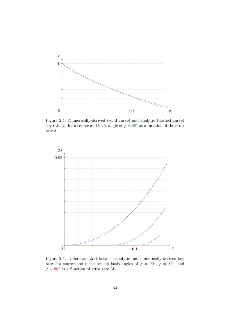
δ
r
0 0.1
1
Figure 2.4: Numerically-derived (solid curve) and analytic (dashed curve)key rate (r) for a source and basis angle of ϕ = 85◦ as a function of the errorrate δ.
δ
∆r
0 0.1
0.08
Figure 2.5: Difference (∆r) between analytic and numerically-derived keyrates for source and measurement-basis angles of ϕ = 90◦, ϕ = 85◦, andϕ = 80◦ as a function of error rate (δ).
64

∆ϕ
δ
0−90◦ 90◦
0.1
Figure 2.6: Threshold error rate (δ) obtained numerically (solid curve) andfor the analytic key rate for deviations ∆ϕ = 90◦ − ϕ from the ideal case.
65

Chapter 3
Security from cloning bounds
This chapter introduces techniques which can be applied to relatively straight-forward security proofs of the BB84 protocol against collective attacks from theprepare-and-measure perspective. The approach can account for imprecisions inboth the source states and Bob’s measurements and can incorporate the localrandomisation preprocessing procedure proposed in [21]. The main result is akey rate for a BB84 implementation in which the source emits four arbitrarypure states (which need not necessarily be qubits) and Bob’s detector is leftuncharacterised. The key rate is shown to be a tight bound on the Devetak-Winter rate with the source characterisation used. With the local randomisationomitted, the key rate closely resembles the Marøy et al. key rate [20].
In addition, more specific secondary results are derived for arbitrary qubit sourcestates using an alternative source characterisation that will be more convenientfor the semi-device-independent protocols studied in the next chapter. Specifi-cally, a key rate is derived for a BB84 implementation emitting arbitrary qubitstates with the detector left uncharacterised on Bob’s side, and an improvedkey rate is derived in the case where both the source and detector are assumedtwo dimensional.
The exposition and results in this chapter are based on Refs. [22, 23].
66

3.1 Introduction
3.1.1 Outline
The previous chapter established the necessity of accounting for device im-precisions in QKD security proofs. This chapter introduces an approachthat can account for such imprecisions in asymptotic security proofs of theprepare-and-measure BB84 protocol against collective attacks. In particu-lar, the source states do not have to satisfy the basis-independence conditionexplained in section 1.2.3.
Most security proofs of the BB84 protocol, and especially those addressingcollective or general attacks, have been developed from the entanglement-based perspective. In some cases where device imprecisions were considered,such as in [49], the result was claimed to account for source imprecisionsin the prepare-and-measure scenario in full generality without noting thebasis-independence limitation. Even the security proofs of the prepare-and-measure BB84 protocol [20, 61, 62] cited in section 1.3.2 that explicitlyrelax the basis-independence condition first recast the BB84 protocol intoan entanglement-based form as a first step in the security analysis. Theauthors of [20, 61], for instance, considered a “virtual” entanglement-basedprotocol in which Alice’s bit and basis choices are both determined by theoutcome of a single four-outcome measurement on an entangled “coin” stateof the form
|Ψ〉 = 1√2
(|z〉|Ψz〉+ |x〉|Ψx〉
), (3.1)
defined in terms of entangled states |Ψz〉 and |Ψx〉 of the form
|Ψz〉 =√p|0〉A|α〉BE
√p′|1〉A|α′〉BE , (3.2)
|Ψx〉 =√q′|+〉A|β〉BE +
√q′|−〉A|β′〉BE . (3.3)
In this virtual protocol, Alice’s measurement in the basis of states |z〉|0〉,|z〉|1〉, |x〉|+〉, and |x〉|−〉 determines which of the four states |α〉, |α′〉, |β〉,and |β′〉 is distributed to Bob (and Eve), and the security proof assumes alower bound on the inner product 〈Ψz|Ψx〉. In this chapter, we will avoidthis detour.
This chapter’s main result is a secret key rate for a BB84 implementationin which the source emits four given but arbitrary pure states and which islargely device-independent on Bob’s side, incorporating the local randomi-sation preprocessing procedure introduced in [21]. The key rate, both withand without local randomisation, is shown to be a tight lower bound on theDevetak-Winter rate with the particular source charaterisation used. For
67

an ideal BB84 source, the previously known threshold error rates of 12.41%and 11%, with and without the preprocessing respectively, are recovered asspecial cases. The key rate without the preprocessing is similar to the keyrate derived by Marøy, Lydersen, and Skaar [20], one of the few previousresults that had accounted for arbitrary imprecisions in both the source anddetector.
Additionally, partially in anticipation of the semi-device-independent pro-tocols studied in the next chapter, a second key rate is derived in the morerestricted case where the source is assumed to emit only arbitrary qubitstates. If Bob’s detector measurements are also assumed two dimensional,the key-rate bound can be further improved to the point that, if no errorsare observed, the key rate is 1.
3.1.2 Scenario and sketch of approach
Here we outline the type of scenario that we will consider and the generalapproach that will be followed in this chapter. We consider a BB84 imple-mentation in which Alice possesses a source which, depending on a choiceof bit and “basis”, emits one of four different quantum states which is sentto Bob. Similar to the notation in the previous chapter, we will consistentlycall the two “z-basis” states |α〉 and |α′〉, and the two “x-basis” states |β〉and |β′〉 (note that this nomenclature is not intended to imply that thesestates are necessarily really the σz and σx eigenstates). We denote thecorresponding density operators by ρ = |α〉〈α|, ρ = |α′〉〈α′|, σ = |β〉〈β|,and σ′ = |β′〉〈β′|. Following a unitary attack by a potential eavesdropper(“Eve”), these states are contained in some Hilbert space HA ⊂ HB ⊗HE,where HB and HE respectively denote the Hilbert spaces accessible to Boband Eve. Upon reception of the states emitted by Alice, Bob performs one oftwo binary-outcome measurements (a “z-basis” or “x-basis” measurement,though we do not assume Bob is necessarily measuring σz or σx) in order tocompute his version of the raw key.
By contrast with the previous chapter, we consider the BB84 variant whereonly the z-basis results are used to generate the key. In this case, as explainedin section 1.4.5, assuming an adversary restricted to collective attacks a lowerbound on the key rate that can securely be extracted by one-way postpro-cessing is given by the Devetak-Winter bound. In the general approachfollowed in this chapter, this problem is broken into two parts.
Section 3.2 first describes how the conditional entropy can be lower boundedin various situations in terms of the fidelity F (ρE, ρ
′E) between the parts of
68

the z-basis states accessible to the adversary. The simplest resulting boundon the key rate, for an unbiased source and without local randomisation, is
r ≥ 1− h(
12 + 1
2F (ρE, ρ′E))− h(δz) , (3.4)
in which the fidelity is defined by F (ρ, σ) = ‖√ρ√σ‖1, h(x) = −x log(x)−
(1 − x) log(1 − x) is the binary entropy, all logarithms are in base 2, andsubscripts indicate partial tracing in the usual way (e.g., ρE = TrB[ρ]).The section also gives a generalisation of (3.4) if Alice randomly flips afraction η of her key bits (the local randomisation preprocessing procedure)and derives a relation for the conditional min-entropy in terms of the tracedistance which will be useful in the next chapter.
In this way, the problem of lower bounding the key rate is generally reducedto lower bounding the fidelity F (ρE, ρ
′E), which is addressed in subsequent
sections of this chapter. We use the fact that Alice and Bob working incooperation can lower bound the trace distances D(ρB, ρ
′B) and D(σB, σ
′B)
in terms of the observed bit error rates via the Helstrom bound (see sec-tion 1.A.2):
D(ρB, ρ′B) ≥ |1− 2δz| , (3.5)
D(σB, σ′B) ≥ |1− 2δx| . (3.6)
The lower bounds for the fidelity will be derived in terms of the trace distanceD(σB, σ
′B) (and, in section 3.5.2, D(ρB, ρ
′B)). Such bounds can be viewed as
a characterisation of the degree to which quantum states can be cloned.
The bounds that will be derived in sections 3.3, 3.4, and 3.5 depend onrelations between the source states |α〉, |α′〉, |β〉, and |β′〉 emitted by thesource. In section 3.4 for instance, similar to the authors of [20, 61] wewill consider the case where the four source states (which may span a four-dimensional Hilbert space in this case) are characterised by a “basis overlap”angle θ, which we define such that√
1 + |sin(θ)| = 12
∣∣〈α|β〉+ 〈α′|β〉+ 〈α|β′〉 − 〈α′|β′〉∣∣ (3.7)
wherever the right-hand side is greater than 1. The cloning bound we willobtain in this case is
F (ρE, ρ′E) ≥ fθ
(D(σB, σ
′B)), (3.8)
with the function fθ defined by
fθ(x) =
{|sin(θ)|x− |cos(θ)|
√1− x2 : x ≥ |cos(θ)|
0 : x ≤ |cos(θ)|, (3.9)
69
which provides a lower bound on F (ρE, ρ′E) wherever the right-hand side of
(3.7) is greater than 1. In this case, substituting (3.8) and D(σB, σ′B) ≥
|1− 2δx| into (3.4), the resulting key rate is
r ≥ 1− h(
12 + 1
2fθ(|1− 2δx|))− h(δz) , (3.10)
which coincides with the key rate given in [20] for this particular scenario.A generalisation of this key rate with local randomisation incorporated willalso be shown to be tight. Section 3.5 will give fidelity bounds in the morerestricted case of a source emitting arbitrary qubit states using a differentsource characterisation than (3.7).
3.2 Conditional entropy bounds
3.2.1 Asymptotic key-rate bound without preprocessing
In this subsection, we derive (3.4). The starting point is the Devetak-Winterbound
r ≥ H(ZA | E)−H(ZA | ZB) . (3.11)
As shown in section 1.4.4, the conditional Shannon entropy H(ZA | ZB),which quantifies the key loss due to error correction, is upper bounded byh(δz) (with equality in the typical case of symmetric errors). The conditionalvon Neumann entropy H(ZA | E) quantifies the amount of key that canbe extracted securely by privacy amplification, which we evaluate on theclassical-quantum state
τZE = 12
(|0〉〈0|Z ⊗ ρE + |1〉〈1|Z ⊗ ρ′E
), (3.12)
where ρ and ρ′ are the z-basis states emitted by Alice, and |0〉Z and |1〉Zdenote the state of a classical register in her possession.
In order to arrive at (3.4), we use that H(ZA | E) ≥ H(ZA | EE′) forany extension of the state (3.12) to a larger Hilbert space HZ ⊗HE ⊗HE′
(formally this follows from the property of strong subadditivity of the vonNeumann entropy [75]). In particular, we use this to replace ρE and ρ′E in(3.12) with purifications |ψ〉 and |ψ′〉 ∈ HE ⊗HE′ . Applying the definitionof the conditional von Neumann entropy, we find
H(ZA | E) ≥ H(ZA | EE′)
= 1− S[
12
(|ψ〉〈ψ|+ |ψ′〉〈ψ′|
)]= 1− h
[12
(1 + |〈ψ|ψ′〉|
)], (3.13)
70

where S(ρ) = −Tr[ρ log(ρ)]. Since by Uhlmann’s theorem we can choose|ψ〉 and |ψ′〉 such that F (ρE, ρ
′E) = |〈ψ|ψ′〉|, we find
H(ZA | E) ≥ 1− h(
12 + 1
2F (ρE, ρ′E)), (3.14)
which completes the derivation of (3.4). Note that (3.14) is equivalent toan analogous bound on the Holevo quantity derived in [76].
The proof given here holds with the assumption that Alice emits the zstates |α〉 and |α′〉 with equal probability. If we wish to account for thepossibility of a biased source, as was considered in [20] for instance, then itis straightforward to adapt the derivation of (3.4). In particular, if the twoz-basis states are emitted with probabilities p = (1+ε)/2 and p′ = (1−ε)/2respectively, (3.14) generalises to
H(ZA | E) ≥ h(p)− h[
12 + 1
2
√ε2 + (1− ε2)F (ρE, ρ
′E)2]. (3.15)
The key rates obtained later will hold essentially unmodified if there is abias in the x basis, provided the observed coincidence statistics are used tocorrectly bound the trace distance D(σB, σ
′B). Note that this is a departure
from the approach used by the authors of [20, 61, 62], where any bias in thesource was included in their analogue of the source characterisation (3.7).This way we obtain a generally better result. For instance, for an otherwiseideal BB84 implementation and in the absence of errors, we obtain the bestpossible key rate of r = h(p).
3.2.2 Incorporating local randomisation
If Alice applies local randomisation, i.e., flips a fraction η of her z-basis keybits, this has the effect of transforming the classical-quantum state (3.12) to
τZE = 12
((1− η)|0〉〈0|Z + η|1〉〈1|Z
)⊗ ρE
+ 12
(η|0〉〈0|Z + (1− η)|1〉〈1|Z
)⊗ ρ′E , (3.16)
which expresses that the z-basis states in Eve’s possession are now correlatedwith a probabilistic mixture of Alice’s (new) z-basis bits. In order to derivea lower bound on H(ZA | E), we first reexpress the classical-quantum state(3.16) as
τZE = 12 |0〉〈0|Z ⊗ ρE + 1
2 |1〉〈1|Z ⊗ ρ′E , (3.17)
where ρE = TrB[ρ] and ρ′E = TrB[ρ′], and we have set
ρ = (1− η)ρ + ηρ′ , (3.18)
ρ′ = ηρ + (1− η)ρ′ , (3.19)
71

The conditional von Neumann entropy, evaluated directly on the classical-quantum state (3.17), simplifies to
H(ZA | E) = 1 + 12
(S(ρE) + S(ρ′E)
)− S
(12(ρE + ρ′E)
), (3.20)
with S(ρ) = −Tr[ρ log(ρ)]. Following the approach in the preceding sub-section, we use that H(ZA | E) ≥ H(ZA | EE′) for any extension τZEE′ ofthe state (3.17) to a larger Hilbert space in order to replace ρE and ρ′E withpurifications |ψ〉 and |ψ′〉 chosen such that F (ρE, ρ
′E) = 〈ψ|ψ′〉. With this
substitution,
H(ZA | E) ≥ 1 + 12S((1− η)|ψ〉〈ψ|+ η|ψ′〉〈ψ′|
)+ 1
2S(η|ψ〉〈ψ|+ (1− η)|ψ′〉〈ψ′|
)− S
(12(|ψ〉〈ψ|+ |ψ′〉〈ψ′|)
). (3.21)
The eigenvalues of the operator (1− η)|ψ〉〈ψ|+ η|ψ′〉〈ψ′| are easily found tobe 1
2 ±12
√1− 4η(1− η)(1− |〈ψ|ψ′〉|2). Consequently,
H(ZA | E) ≥ 1− h(
12 + 1
2F (ρE, ρ′E))
+ h(
12 + 1
2
√1− 4η(1− η)
(1− F (ρE, ρ
′E)2)). (3.22)
In appendix 3.A, the right-hand side of (3.22) is shown to be an increasingfunction of the fidelity. Given a lower bound F (ρE, ρ
′E) ≥ Fz on the fidelity,
then, we obtain the analytic lower bound
r ≥ 1 + h(
12 + 1
2
√1− 4η(1− η)
(1− F 2
z
))− h(
12 + 1
2Fz
)− h((1− η)δz + η(1− δz)
)(3.23)
for the key rate.
The best result for the key rate is obtained by maximising the right-hand sideof (3.23) over η, which, if necessary, is readily done numerically. Typically,as the channel noise approaches the maximal threshold, the optimal fractionη approaches 1/2. In this regime, the behaviour of the key-rate bound can bestudied by substituting η = (1−ε)/2 and expanding the resulting expressionin powers of ε. The result, to the first non-trivial order in ε, is
r &
(−1− F 2
z
4Fzlog
(1 + Fz
1− Fz
)+
(1− 2δz)2
2 ln(2)
)ε2 , (3.24)
where ln is the natural logarithm. Consequently, threshold error rates canbe obtained by identifying corresponding roots of the expression(
1− F 2z
)ln
(1 + Fz
1− Fz
)− 2Fz(1− 2δz)
2 . (3.25)
72

3.2.3 Bounding the min-entropy
As alluded to above, the Devetak-Winter bound, and consequently thebound (3.4) on the key rate that we will use in the remainder of this thesis,is only guaranteed to hold in the asymptotic limit of an infinitely long key.In the realistic finite-key case, a finite-key result can be derived based on a“one shot” version of the Devetak-Winter rate [60] where the main problemin obtaining a security proof is reduced to lower bounding the conditionalmin-entropy Hmin(ZA | E) [77], defined by
Hmin(ZA | E) = maxσE
sup{λ ∈ R : 2−λ1Z ⊗ σE ≥ τZE
}, (3.26)
rather than the von Neumann entropy H(ZA | E). To obtain a resultthat converges asymptotically to the key rate given by the Devetak-Winterbound, the min-entropy should ideally be evaluated with a smoothing pa-rameter, which can roughly be interpreted as a small additional probabilityof failure traded in exchange for a higher key rate, and which can be madearbitrarily small in the asymptotic limit. We refer to [49, 78] for a discussionof the details.
Whether and how the smooth min-entropy can be bounded in such a way asto recover (3.14) asymptotically will be left as a problem for future work andwill not be further addressed. Here, we show that the min-entropy (withoutsmoothing), which in any case may be useful as a lower bound on the vonNeumann entropy, has an exact expression in terms of the trace distance.To obtain this, we insert the expression (3.12) for τZE into the condition2−λ1Z ⊗ σE − τZE ≥ 0 appearing in (3.26). This expands to
|0〉〈0|Z ⊗(2−λσE − 1
2ρE
)+ |1〉〈1| ⊗
(2−λσE − 1
2ρ′E
)≥ 0 , (3.27)
from which we extract the conditions 21−λσE ≥ ρE and 21−λσE ≥ ρ′E. Thetightest fit is obtained with
21−λσE = 12(ρE + ρ′E) + 1
2 |ρE − ρ′E| . (3.28)
We determine λ = Hmin(ZA | E) by taking the trace of both sides:
21−λ = 1 + 12 Tr
[|ρE − ρ′E|
]= 1 +D(ρE, ρ
′E) , (3.29)
which rearranges to
Hmin(ZA | E) = 1− log(1 +D(ρE, ρ
′E)). (3.30)
The end result (3.30) is a special case of the min-entropy’s expression interms of the guessing probability [77]. Applying the bound D(ρE, ρ
′E) ≤
73

√1− F (ρE, ρ
′E)2, we can alternatively bound the min-entropy in terms of
the fidelity. While the result would be less than optimal and still limitedto collective attacks, it is worth noting that using (3.30) in place of (3.14)would already allow the obtention of finite-key bounds using the generalapproach explored in this chapter.
3.3 BB84 with ideal source
In the special case of an ideal BB84 source, characterised by θ = π/2, thegeneral cloning bound (3.8) reduces to
F (ρE, ρ′E) ≥ D(σB, σ
′B) , (3.31)
and we recover the famous key rate r ≥ 1 − h(δx) − h(δz) due to Shor andPreskill [53]. While the proof of (3.8) is not complicated, a direct proof of(3.31) is especially simple and will serve to introduce our techniques.
In an ideal BB84 implementation, the source states form two mutually un-biased orthogonal bases, i.e., satisfy
〈α|α′〉 = 〈β|β′〉 = 0 (3.32)
and, in an appropriate phase convention,
|α〉 = 1√2
(|β〉+ |β′〉
),
|α′〉 = 1√2
(|β〉 − |β′〉
). (3.33)
Equivalently, one can identify Z = ρ − ρ′ and X = σ − σ′ with the Pauli zand x operators. With this notation, D(ρB, ρ
′B) = 1
2‖ZB‖1 and D(σB, σ′B) =
12‖XB‖1.
We obtain (3.31) as follows. Let UB be the (Hermitian) unitary operatoracting on HB such that 1
2‖XB‖1 = 12 TrB[UBXB]. Then,
D(σB, σ′B) = 1
2 TrB[UBXB]
= 12 Tr
[(UB ⊗ 1E)
]= 1
2
(〈α|UB ⊗ 1E|α′〉+ 〈α′|UB ⊗ 1E|α〉
)= Re
[〈α|UB ⊗ 1E|α′〉
]≤∣∣〈α|UB ⊗ 1E|α′〉
∣∣ . (3.34)
Now, |α〉 and |α′〉 are by definition purifications of ρE and ρ′E, and since UB⊗1E acts nontrivially only on HB, the state UB ⊗ 1E|α′〉 is still a purification
74
of ρ′E. Thus, by Uhlmann’s theorem, the last line of (3.34) provides a lowerbound on the fidelity between ρE and ρ′E, which concludes our proof. Notethat, similar to the derivation in section 1.4.4, we never actually used theorthogonality relations in the proof above, meaning that the proof also holdsfor the entanglement-based BB84 variant.
We conclude this discussion of the ideal BB84 scenario by noting that (3.31)can be seen as a strengthened version the tradeoff relation,
D(ρE, ρ′E)2 +D(σB, σ
′B)2 ≤ 1 . (3.35)
cited as a corollary of the derivation of the FGGNP bound summarisedin section 1.4.4. Specifically, (3.35) follows by applying the upper boundD(ρE, ρ
′E) ≤
√1− F (ρE, ρ
′E)2 to (3.31).
3.4 BB84 with arbitrary source states
3.4.1 Derivation of fidelity bound
We now derive (3.8). Our starting point is the quantity
∆ = 12√
2
(〈α|β〉+ 〈α′|β〉+ 〈α|β′〉 − 〈α′|β′〉
). (3.36)
Note that (3.36) as expressed above is dependent on physically irrelevantphase factors (e.g. |α〉 and eiφ|α〉 denote the same state); to obtain the bestresult, one should adopt the phase convention that maximises (3.36), whichcan then always be taken to be real.
Let P and Q be orthogonal projectors such that P −Q = U and P +Q = 1,where U = UB ⊗ 1E is the Hermitian unitary such that 1
2 Tr[U(σ − σ′)] =D(σB, σ
′B), as in the proof of (3.31). For convenience, we also define the
(generally not normalised) states |α±〉 = (|α〉 ± |α′〉)/√
2. Then,
2∆ = 〈α+|(P +Q)|β〉+ 〈α−|(P +Q)|β′〉≤ |〈α+|P |β〉|+ |〈α+|Q|β〉|
+ |〈α−|P |β′〉|+ |〈α−|Q|β′〉| . (3.37)
Applying the Cauchy-Schwarz inequality twice on the first and fourth termson the right-hand side,
|〈α+|P |β〉|+ |〈α−|Q|β′〉|≤√〈α+|P |α+〉
√〈β|P |β〉+
√〈α−|Q|α−〉
√〈β′|Q|β′〉
≤√〈α+|P |α+〉+ 〈α−|Q|α−〉
√〈β|P |β〉+ 〈β′|Q|β′〉
=√
1 + Re[〈α|U |α′〉]√
1 +D(σB, σ′B) . (3.38)
75

In a similar manner, |〈α+|Q|β〉| + |〈α−|P |β′〉| provides a lower bound on√1− Re[〈α|U |α′〉]
√1−D(σB, σ
′B). We thus obtain
∆ ≤√
12 + 1
2 Re[〈α|U |α′〉]√
12 + 1
2D(σB, σ′B)
+√
12 −
12 Re[〈α|U |α′〉]
√12 −
12D(σB, σ
′B) , (3.39)
where Re[〈α|U |α′〉] in turn provides a lower bound on F (ρE, ρ′E), as in the
proof of (3.31). Substituting ∆ =√
1 + |sin(θ)|/√
2 and rearranging, wearrive at (3.8).
3.4.2 Resulting key rate
Explicitly combining these with the generic key-rate expression (3.23), weobtain the bound
r ≥ 1 + h(
12 + 1
2
√1− 4η(1− η)
(1− fθ(|1− 2δx|)2
))− h(
12 + 1
2fθ(|1− 2δx|))− h(δz) , (3.40)
with δz = (1− η)δz + η(1− δz) and fθ defined by
fθ(x) =
{|sin(θ)|x− |cos(θ)|
√1− x2 : x ≥ |cos(θ)|
0 : x ≤ |cos(θ)|, (3.41)
for the key rate with local randomisation applied. For η = 0, we recover thekey rate
r ≥ 1− h(
12 + 1
2fθ(|1− 2δx|))− h(δz) (3.42)
given earlier, which itself coincides with the rate derived in [20] in the settingunder consideration here.
The rates (3.40) and (3.42) (with and without local randomisation, respec-tively) are illustrated for a few values of θ in figure 3.1, assuming symmetricerrors (i.e., δz = δx = δ) for simplicity. The depicted rates with localrandomisation were found by numerically maximising (3.40) over η. Forθ = π/2 = 90◦, corresponding to an ideal BB84 source, we recover the Shor-Preskill rate [53] and the improvement with local randomisation depicted infigure 2 of Ref. [32].
The threshold error rates, i.e., the error rates for which the key rates (3.42)without preprocessing and (3.40) with optimal local randomisation becomezero, again for δz = δx = δ, are depicted in figure 3.2 as a function of θ.The threshold curve with local randomisation was found by identifying the
76

δ
r
0 0.1
1
Figure 3.1: Key rate (3.40) secure against collective attacks for a BB84implementation of source characterisation angle θ = 90◦, θ = 80◦, and θ =70◦, with (dashed curves) and without (solid curves) local randomisation,for δ = δz = δx.
θ
δ
0 90◦
0.1
Figure 3.2: Threshold error rate, i.e., the error rate δ = δz = δx for which thekey-rate bound (3.40) becomes zero, with (dashed curve) and without (solidcurve) local randomisation, for source characterisation angles 0 ≤ θ ≤ 90◦.
77

corresponding root of (3.25). For θ = π/2 = 90◦ we recover the thresholderror rates of δ ≈ 12.4120% and δ ≈ 11.0028% originally found in Refs. [21]and [53], respectively. For an ideal BB84 implementation, this correspondsto a relative increase of around 12.81% to the provably tolerable channelnoise. This difference becomes more significant as θ decreases: for instancethe relative improvement becomes around 20.00% (δ ≈ 7.5191% comparedwith δ ≈ 6.2660%) for θ = 70◦, around 33.84% (δ ≈ 3.1120% vs δ ≈2.3251%) for θ = 45◦, and around 83.38% (δ ≈ 0.1538% vs δ ≈ 0.08390%)if θ is as low as 10◦, indicating that the benefit of additional preprocessingbecomes more pronounced for a realistic BB84 implementation expected tosuffer from device imprecisions.
Finally, if dimHA = 2 and the source states form two orthogonal bases, thenθ as defined by (3.7) coincides with the angle separating the bases on theBloch sphere. In this particular case, the source is basis independent (i.e.,12ρ+ 1
2ρ′ = 1
2σ+ 12σ′), and we note that the key rate (3.42) is an improvement
over the key rate predicted by the uncertainty relation [59, 60], which forcomparison is
r ≥ 1− log(1 + |cos(θ)|)− h(δx)− h(δz) . (3.43)
3.4.3 Optimality
For the nonideal BB84 implementation considered in the preceding section,the key-rate bound (3.40) is tight in the sense that the Devetak-Winterrate (3.11) can be attained for all values of the independent variables θ,δz, δx, and η. This is demonstrated here by the explicit construction of afamily of source states and optimal unitary attacks. Equality between theright-hand sides of (3.11) and (3.40) requires the conditional von Neumannentropy bound (3.22) and the fidelity bound (3.8) to hold with equalitysimultaneously, which helps in the determination of an optimal attack. First,note that in the case of an equality, (3.8) rearranges to
|sin(θ)| = FzDx +√
1− F 2z
√1−D 2
x , (3.44)
with Fz = F (ρE, ρ′E) and Dx = D(σB, σ
′B) and the condition Fz ≤ Dx.
Equation (3.44) can equivalently be reexpressed as√1 + |sin(θ)| = 1√
2
(√1 + Fz
√1 +Dx +
√1− Fz
√1−Dx
). (3.45)
Consequently, our goal will be to construct source states such that the defini-tion of the source characterisation (3.7) equals the right-hand side of (3.45).
78

Requiring D(ρB, ρ′B) = Dz suggests setting the z-basis states to the form
|α〉 =√
1+Dz2 |0〉B|ψ0〉E +
√1−Dz
2 |1〉B|ψ′1〉E , (3.46)
|α′〉 =√
1−Dz2 |0〉B|ψ1〉E +
√1+Dz
2 |1〉B|ψ′0〉E , (3.47)
with |0〉B and |1〉B orthonormal. The trace distance D(ρB, ρ′B) will equal
Dz if 〈ψ0|ψ′1〉 = 〈ψ1|ψ′0〉 = 0. In order for the fidelity F (ρE, ρ′E) to equal
Fz, and in such a way that the von Neumann entropy bound (3.22) be-comes an equality, we additionally require 〈ψ0|ψ1〉 = 〈ψ′0|ψ′1〉 = 0 and〈ψ0|ψ′0〉 = 〈ψ1|ψ′1〉 = Fz ∈ R+, such that {|ψ0〉, |ψ′0〉} and {|ψ1〉, |ψ′1〉} spantwo mutually orthogonal subspaces. Note that, with these definitions, |α〉and |α′〉 are normalised and orthogonal.
The right-hand side of the source characterisation (3.7) can be reexpressedas 1√
2
∣∣〈α+|β〉 + 〈α−|β′〉∣∣ with |α±〉 = 1√
2
(|α〉 ± |α′〉
). Introducing, for con-
venience, the states
|αk〉 = |0〉B|ψk〉E , |α′k〉 = |1〉B|ψ′k〉E , (3.48)
and |α±k 〉 = 1√2
(|αk〉 ± |α′k〉
), k ∈ {0, 1}, we find
|α+k 〉 =
√1+Fz
2 |+〉B|ψ+k 〉E +
√1−Fz
2 |−〉B|ψ−k 〉E , (3.49)
|α−k 〉 =√
1−Fz2 |+〉B|ψ
−k 〉E +
√1+Fz
2 |−〉B|ψ+k 〉E , (3.50)
where |±〉B = 1√2
(|0〉B + |1〉B
)and the states
|ψ±k 〉E =|ψk〉E ± |ψ′k〉E√
2± 2Fz(3.51)
are orthonormal. In terms of |α±k 〉,
|α+〉 =√
1+Dz2 |α
+0 〉+
√1−Dz
2 |α+1 〉 , (3.52)
|α−〉 =√
1+Dz2 |α
−0 〉 −
√1−Dz
2 |α−1 〉 . (3.53)
It is then fairly straightforward to construct x-basis states for which theright-hand side of the source characterisation (3.7) will take the form of theright-hand side of (3.45). We set
|βk〉 =√
1+Dx2 |+〉B|ψ+
k 〉E +√
1−Dx2 |−〉B|ψ−k 〉E , (3.54)
|β′k〉 =√
1−Dx2 |+〉B|ψ−k 〉E +
√1+Dx
2 |−〉B|ψ+k 〉E , (3.55)
79

and
|β〉 =√
1+Dz2 |β0〉+
√1−Dz
2 |β1〉 , (3.56)
|β′〉 =√
1+Dz2 |β
′0〉 −
√1−Dz
2 |β′1〉 . (3.57)
With these definitions we find
〈α+|β〉 = 〈α−|β′〉 =1
2
(√1 + Fz
√1 +Dx +
√1− Fz
√1−Dx
), (3.58)
independently of Dz, from which we recover the right-hand side of the rear-rangement (3.45) of the fidelity bound (3.8).
Explicitly, from the expressions (3.46), (3.47), (3.56), and (3.57) for the z-and x-basis states, Bob’s marginals are given by
ρB = 1+Dz2 |0〉〈0|B + 1−Dz
2 |1〉〈1|B , (3.59)
ρ′B = 1−Dz2 |0〉〈0|B + 1+Dz
2 |1〉〈1|B , (3.60)
σB = 1+Dx2 |+〉〈+|B + 1−Dx
2 |−〉〈−|B , (3.61)
σ′B = 1−Dx2 |+〉〈+|B + 1+Dx
2 |−〉〈−|B . (3.62)
Consequently, Alice and Bob detect errors at the rates δz = 12 −
12Dz and
δx = 12 −
12Dx if Bob measures (optimally) in the σz and σx bases. Likewise,
Eve’s marginals of the z states are given by
ρE = 1+Dz2 |ψ0〉〈ψ0|E + 1−Dz
2 |ψ′1〉〈ψ′1|E , (3.63)
ρ′E = 1−Dz2 |ψ1〉〈ψ1|E + 1+Dz
2 |ψ′0〉〈ψ′0|E , (3.64)
for which one can readily verify that F (ρE, ρ′E) = ‖
√ρE
√ρ′E‖1 = Fz and,
for any p, q ≥ 0 and p+ q = 1,
S(pρE + qρ′E
)= h
(12 + 1
2Dz
)+ 1+Dz
2 S(p|ψ0〉〈ψ0|E + q|ψ′0〉〈ψ′0|E
)+ 1−Dz
2 S(p|ψ′1〉〈ψ′1|E + q|ψ1〉〈ψ1|E
)= h
(12 + 1
2Dz
)+ h(
12 + 1
2
√1− 4pq(1− F 2
z )). (3.65)
Using (3.65) to directly evaluate the expression (3.20) for the conditionalvon Neumann entropy H(ZA | E), we find that its bound (3.22) in terms offidelity F (ρE, ρ
′E) is attained with equality for the entire family of sources
and attacks just constructed.
Equations (3.46), (3.47), (3.56), and (3.57) give the optimal attack for afamily of sources identified by the relations
〈α|α′〉 = 〈β|β′〉 = 0 (3.66)
80

and
〈α|β〉 = 〈α′|β〉 = 〈α|β′〉 = −〈α′|β′〉 =
√1+|sin(θ)|
2 , (3.67)
for which the bound (3.40) on the Devetak-Winter rate is attained withequality independently of the fraction η of bits flipped by Alice in the localrandomisation preprocessing step. The family of optimal attacks given heregeneralises the optimal individual attack derived for an ideal BB84 source in[14], which is recovered for |sin(θ)| = 1 or, equivalently, by setting Fz = Dx.Another extreme worth noting is the case Fz = 0 and Dz = Dx = 1, inwhich case |sin(θ)| = 0 and
|α〉 = |0〉B|0〉E , |α′〉 = |1〉B|1〉E , (3.68)
|β〉 = |+〉B|+〉E , |β′〉 = |−〉B|+〉E , (3.69)
i.e., the adversary acquires perfect copies of Bob’s z-basis states withoutintroducing any errors.
3.5 BB84 with arbitrary qubit states
3.5.1 Arbitrary measurements
We now turn to a more detailed study of qubit sources. It will be convenientto characterise such a source in terms of three parameters: an angle ϕrepresenting the angle between the two bases on the Bloch sphere, and anglesα and β measuring the nonorthogonality of the states constituting eachbasis and defined by |sin(α)| = |〈α|α′〉| and |sin(β)| = |〈β|β′〉| respectively.With this characterisation, the differences between the z- and x-basis densityoperators can be expressed as
ρ− ρ′ = cos(α)Z , (3.70)
σ − σ′ = cos(β)X , (3.71)
where Z and X are Pauli-type operators (i.e., two dimensional and of eigen-values +1 and −1) and separated by an angle ϕ on the Bloch sphere suchthat their anticommutator satisfies 1
2{Z, X} = cos(ϕ)1A.
In order to bound the distinguishability between ρE and ρ′E, we first intro-duce another Pauli-type operator W orthogonal to Z on the Bloch sphereand in the same plane as Z and X in such a way that X can be expressedas
X = cos(ϕ)Z + sin(ϕ)W . (3.72)
81

With a suitable choice of basis, Z and W can be identified with σz andσx, respectively. The trace norm 1
2‖WB‖1 is a priori unknown, since it isnot the difference between two states that are actually prepared by Alice ormeasured by Bob. It can, however, be bounded in terms of 1
2‖XB‖1, which isin turn lower bounded in terms of the x-basis error rate. To see this, similarto the preceding subsections, let U = UB ⊗ 1E be the Hermitian unitaryoperator such that 1
2‖XB‖1 = 12 Tr[UX]. Then,
12‖XB‖1 = 1
2
∥∥cos(ϕ)ZB + sin(ϕ)WB
∥∥1
≤ |cos(ϕ)|12∣∣Tr[UZ]
∣∣+ |sin(ϕ)|12∣∣Tr[UW ]
∣∣≤ |cos(ϕ)|
√1− 1
4 Tr[UW ]2 + |sin(ϕ)|12∣∣Tr[UW ]
∣∣ , (3.73)
where we used that 14 Tr[UZ]2 + 1
4 Tr[UW ]2 ≤ 1. Rearranging the final lineand using 1
2
∣∣Tr[UW ]∣∣ as a lower bound on 1
2‖WB‖1, we obtain
12‖WB‖1 ≥ |sin(ϕ)|12‖XB‖1 − |cos(ϕ)|
√1− 1
4‖XB‖12 . (3.74)
Since 12‖WB‖1 is also necessarily positive, the lower can be expressed as
12‖WB‖1 ≥ fϕ
(12‖XB‖1
), (3.75)
where f is the same function earlier defined in (3.41), except that we usethe angle ϕ between the bases in place of the basis overlap angle θ definedin (3.7).
If we are content with obtaining a lower bound on the min-entropy, whichdepends on the trace distance D(ρE, ρ
′E) we simply use that D(ρE, ρ
′E) =
|cos(α)|12‖ZE‖1. Using that 14‖ZE‖12+ 1
4‖WB‖12 ≤ 1, which was first derivedin section 1.4.4 and recovered as (3.35) in section 3.3, 1
2‖ZE‖1 can be upperbounded by
12‖ZE‖1 ≤ |cos(ϕ)|‖XB‖1 + |sin(ϕ)|
√1− 1
4‖XB‖12 , (3.76)
provided that 12‖XB‖1 ≥ |cos(ϕ)|.
Deriving a lower bound on the conditional von Neumann entropy via itslower bound on the fidelity F (ρE, ρ
′E) requires additional work. If |α〉 and |α′〉
happen to be orthogonal, i.e., if sin(α) = 0, then according to (3.31) Eve’sfidelity is simply bounded by F (ρE, ρ
′E) ≥ 1
2‖WB‖1. This, however, doesnot hold more generally: a numerical minimisation of F (ρE, ρ
′E) − 1
2‖WB‖1will easily find counterexamples. Nor is this an artefact of bounding thefidelity as an intermediate step in bounding the key rate, as one can likewisefind cases where H(ZA | E) � 1 − h
(12 + 1
4‖WB‖1)
when minimising theconditional von Neumann entropy directly.
82

It follows that a generally valid bound will depend explicitly on the non-orthogonality measured by the angle α. In the following, we will show that
F (ρE, ρ′E) ≥ gα
(12‖WB‖1
), (3.77)
with the function gα defined by
gα(x) =
{(1 + |sin(α)|)x− |sin(α)| : x ≥ 2|sin(α)|
1+|sin(α)||sin(α)| : x ≤ 2|sin(α)|
1+|sin(α)|. (3.78)
Combining (3.75) and (3.77), we obtain
F (ρE, ρ′E) ≥ gα ◦ fϕ
(D(σB,σ
′B)
|cos(β)|
), (3.79)
where we have used that σ − σ′ = cos(β)X. We see here that explicitlyintroducing the non-orthogonality of the x-basis states can only improve thekey rate bound. This is not surprising since the x-basis states are only usedfor the purpose of testing the channel. Explicitly writing the resulting keyrate,
r ≥ 1− h[
12 + 1
2gα ◦ fϕ(|1−2δx||cos(β)|
)]− h(δz) . (3.80)
The remainder of this section will be devoted to the determination of thefunction gα. We first express |α〉 and |α′〉 as
|α〉 = cos(α2 )|z〉+ eiφ sin(α2 )|z′〉 , (3.81)
|α′〉 = sin(α2 )|z〉+ eiφ cos(α2 )|z′〉 (3.82)
in terms of the (orthogonal) eigenstates |z〉 and |z′〉 of the operator Z definedat the beginning of this subsection, such that 〈α|α′〉 = sin(α) and ρ − ρ′ =cos(α)
(|z〉〈z| − |z′〉〈z′|
). We define the Hermitian unitary U = UB⊗1E such
that 12‖WB‖1 = 1
2 Tr[UW ] = Re[〈z|U |z′〉]. Without loss of generality, we cantake the quantity Γ = 〈z|U |z′〉 to be real (if necessary, this can be achievedby absorbing its phase into the phase φ already present in (3.81)). A lowerbound is already given by
F (ρE, ρ′E) ≥
∣∣〈α|U |α′〉∣∣ , (3.83)
however the result this would produce is not optimal. In order to obtain abetter result, note that any unitary of the form UB⊗1E can be used in placeof U in (3.83). In particular, since U is Hermitian, the family of operators
U(γ) = i sin(γ)1+ cos(γ)U (3.84)
83

are unitary and satisfy this requirement. Evaluating 〈α|U(γ)|α′〉, we find
〈α|U(γ)|α′〉 = 12 sin(α)
(〈z|U(γ)|z〉+ 〈z′|U(γ)|z′〉
)+ eiφ cos(α2 )2〈z|U(γ)|z′〉+ e−iφ sin(α2 )2〈z′|U(γ)|z〉
= i sin(γ) sin(α) + cos(γ) sin(α)K
+ cos(γ)(cos(φ) + i cos(α) sin(φ)
)Γ , (3.85)
where we have set K = 12(〈z|U |z〉+ 〈z′|U |z′〉). Squaring the last line,∣∣〈α|U(γ)|α′〉
∣∣2 = cos(γ)2(sin(α)K + cos(φ)Γ
)2+(sin(γ) sin(α) + cos(γ) cos(α) sin(φ)Γ
)2. (3.86)
Our task now is to maximise this quantity over γ and minimise over possiblevalues of K and φ. We begin by minimising over K for fixed γ and φ. First,note that |K|+Γ ≤ 1 (this can be inferred by evaluating (3.86) for γ = φ = 0and α = ±π/2 and noting that the result should never exceed 1). With thisconstraint, we wish to minimise Q = |sin(α)K+ cos(φ)Γ|. If Γ is sufficientlysmall, we are able to choose K such that this quantity is zero. Otherwise,we simply set |K| = 1 − Γ. Calling Q∗ the minimum possible value of|sin(α)K + cos(φ)Γ|, we have
Q∗ =
{(|sin(α)|+ |cos(φ)|
)Γ− |sin(α)| : Γ ≥ |sin(α)|
|sin(α)|+|cos(φ)|0 : Γ ≤ |sin(α)|
|sin(α)|+|cos(φ)|, (3.87)
The next step is the maximisation over γ. Since Q∗ has no dependence onγ, this is straightforward. For the optimal value γ∗ of γ, we find∣∣〈α|U(γ∗)|α′〉
∣∣2 = 12
(Q 2∗ + cos(α)2 sin(φ)2Γ2 + sin(α)2
)+ 1
2
{(Q 2∗ + cos(α)2 sin(φ)2Γ2 − sin(α)2
)2+ 4 sin(α)2 cos(α)2 sin(φ)2Γ2
}1/2. (3.88)
Finally, we minimise over φ. For values of φ such that |cos(φ)| ≤ |sin(α)|1−ΓΓ ,
we set Q∗ = 0, and (3.88) simplifies to∣∣〈α|U(γ∗)|α′〉∣∣2 = sin(α)2 + cos(α)2 sin(φ)2Γ2 . (3.89)
If Γ ≤ |sin(α)|1+|sin(α)| , then Q∗ = 0 regardless of φ, and the minimum of (3.89) is∣∣〈α|U(γ∗)|α′〉
∣∣ = |sin(α)| . (3.90)
84

Otherwise, the minimum of (3.86) for values of φ where Q∗ = 0 is found byusing the minimum allowed value of |sin(φ)| in (3.89), which simplifies to∣∣〈α|U(γ∗)|α′〉
∣∣ = sin(α)2 + cos(α)2Γ . (3.91)
If Γ > |sin(α)|1+|sin(α)| , then we must separately consider the range of possible val-
ues of φ for which |cos(φ)| > |sin(α)|1−ΓΓ , where Q∗ = (|sin(α)|+ |cos(φ)|)−
|sin(α)|. We have
Q 2∗ + cos(α)2 sin(φ)2Γ2 = Y Γ(Y Γ− 2) + 2 cos(α)2Γ + sin(α)2 , (3.92)
where we have set Y = 1 + |sin(α)||cos(φ)|. Then,∣∣〈α|U(γ∗)|α′〉∣∣2 = sin(α)2 + cos(α)2Γ + 1
2Y Γ(Y Γ− 2)
+ 12Γ((Y (Y Γ− 2) + 2 cos(α)2
)2+ 4 sin(α)2 cos(α)2 sin(φ)2
)1/2, (3.93)
which we can simplify down to∣∣〈α|U(γ∗)|α′〉∣∣2 = sin(α)2 + cos(α)2Γ + 1
2Y Γ(Y Γ− 2)
+ 12Y Γ
√(Y Γ− 2)2 + 4 cos(α)2(Γ− 1) . (3.94)
This is a decreasing function in Y and is therefore minimised by taking|cos(φ)| = 1, or Y∗ = 1 + |sin(α)|. We find∣∣〈α|U(γ∗)|α′〉
∣∣2 = sin(α)2 + cos(α)2Γ
+ 12Y∗Γ
[Y∗Γ− 2 +
∣∣Y∗Γ− 2|sin(α)|∣∣] . (3.95)
If Γ ≥ 2|sin(α)|1+|sin(α)| , then the minimum we find is∣∣〈α|U(γ∗)|α′〉
∣∣ =(1 + |sin(α)|
)Γ− |sin(α)| . (3.96)
Otherwise, the minimum is simply |sin(α)|. Since (3.96) is always less than(3.91), our final result is
∣∣〈α|U(γ∗)|α′〉∣∣ ≥ {(1 + |sin(α)|
)Γ− |sin(α)| : Γ ≥ 2|sin(α)|
1+|sin(α)||sin(α)| : Γ ≤ 2|sin(α)|
1+|sin(α)|. (3.97)
Recalling that F (ρE, ρ′E) ≥ |〈α|U(γ∗)|α′〉| and that we defined Γ = 1
2‖WB‖1,this concludes the proof of (3.77).
85

3.5.2 Qubit source and detector
In most security analyses of the BB84 protocol accounting for device align-ment errors, including the results derived in sections 3.4 and 3.5.1, only thex-basis error rate is used to bound the information an eavesdropper couldhave about the key. This leaves open the possibility that we could derivebetter results if the z-basis error rate were also used for this purpose. Here,we will illustrate how such a result can be derived in the case where Al-ice’s source emits qubit states and Bob’s detector is assumed to performtwo-dimensional measurements.
As in section 3.5.1, we take ρ−ρ′ ∝ Z and σ−σ′ ∝ X, where X = cos(ϕ)Z+sin(ϕ)W , and Z and W can be identified with the Pauli z and x operators.The error rates provide lower bounds on D(ρB, ρ
′B) = |cos(α)|12‖ZB‖1 and
D(σB, σ′B) = |cos(β)|12‖XB‖1. The main intuition for deriving an improved
key rate is that, if dimHB = 2, the quantities 12‖ZB‖1, 1
2‖XB‖1, and 12‖WB‖1
are constrained in the values they can take. Specifically, we will be able toshow that√
1− 14‖XB‖ 2
1 ≥ |sin(ϕ)|√
1− 14‖WB‖ 2
1 − |cos(ϕ)|√
1− 14‖ZB‖ 2
1 . (3.98)
Since we have F (ρE, ρ′E) ≥ gα
(12‖WB‖1
)from (3.77), (3.98) provides a sec-
ond bound on the fidelity to complement (3.79). Our end result is similarin form to (3.79):
F (ρE, ρ′E) ≥ gα ◦ f (2)
ϕ
(D(ρB,ρ
′B)
|cos(α)| ,D(σB,σ
′B)
|cos(β)|
), (3.99)
with the function f(2)ϕ defined piecewise by
f (2)ϕ (z, x) =
{hϕ(z, x) : q(z, x) ≥ |cos(ϕ)|fϕ(x) : q(z, x) ≤ |cos(ϕ)|
, (3.100)
in turn with hϕ defined such that
|sin(ϕ)|√
1− hϕ(z, x)2 =√
1− x2 + |cos(ϕ)|√
1− z2 , (3.101)
fϕ as in (3.41), and q by
q(z, x) = zx−√
(1− z2)(1− x2) . (3.102)
The resulting key rate is
r ≥ 1− h[
12 + 1
2gα ◦ f(2)ϕ
(|1−2δz||cos(α)| ,
|1−2δx||cos(β)|
)]− h(δz) . (3.103)
86
We note that, provided sin(ϕ) 6= 0, if 12‖ZB‖1 = 1 and 1
2‖XB‖1 = 1 then(3.98) implies 1
2‖WB‖1 = 1. Thus, except in the pathological case where thez and x bases coincide, if δz = (1 − |cos(α)|)/2 and δx = (1 − |cos(β)|)/2(the minimum possible error rates) we certify that Bob is in full control ofAlice’s source space and we find H(ZA | E) = 1 and r ≥ 1− h(δz) (i.e., theonly reduction in the key rate is due to error correction).
We now prove (3.98). Our strategy will be to derive an upper bound on12‖XB‖1 given 1
2‖ZB‖1 and 12‖WB‖1, and then invert the resulting bound
for 12‖WB‖1. Where HB is two dimensional, this is especially easy as all
three operators are expressible as combinations of Pauli operators. We setZB = z · σ, XB = x · σ, and WB = w · σ, with ‖z‖, ‖x‖, ‖v‖ ≤ 1. Forsimplicity of notation we will generally denote by e.g. a the norm ‖a‖ of avector a. Because a = ‖a‖ = 1
2‖a·σ‖1, deriving the desired bound is reducedto bounding x in terms of z and w. Using that XB = cos(ϕ)ZB + sin(ϕ)WB,we have
x = 12‖XB‖1
= 12‖cos(ϕ)ZB + sin(ϕ)WB‖1
= ‖cos(ϕ)z + sin(ϕ)w‖ . (3.104)
Squaring this and developing,
x2 = 12(z2 + w2) + 1
2 cos(2ϕ)(z2 − w2) + sin(2ϕ)w · z . (3.105)
Now, while we are working with a given value of ϕ, we can arrive at anontrivial bound on x by noting that 1
2‖cos(ϕ)ZB + sin(ϕ)WB‖1 must beless than 1 for all values of ϕ. The maximum value of (3.105), if ϕ isallowed to take any value, is given by
x 2max = 1
2(z2 + w2) +√
14(z2 − w2)2 + (w · z)2 . (3.106)
Requiring that the right-hand side is less than 1, we find
(2− z2 − w2)2 ≥ (z2 − w2)2 + 4(w · z)2 , (3.107)
which simplifies to|w · z| ≤
√(1− z2)(1− w2) . (3.108)
From this, we deduce that
x2 ≤ 12(z2 +w2)+ 1
2 cos(2ϕ)(z2−w2)+|sin(2ϕ)|√
(1− z2)(1− w2) , (3.109)
or equivalently,√1− x2 ≥
∣∣|cos(ϕ)|√
1− z2 − |sin(ϕ)|√
1− w2∣∣ . (3.110)
87

Invoking the triangle inequality on (3.104), we also trivially have
x ≤ |cos(ϕ)|z + |sin(ϕ)|w (3.111)
andx ≥
∣∣|cos(ϕ)|z − |sin(ϕ)|w∣∣ . (3.112)
Inverting these, we find two lower bounds on w:
|sin(ϕ)|√
1− w2 ≤√
1− x2 + |cos(ϕ)|√
1− z2 (3.113)
and|sin(ϕ)|w ≥
∣∣x− |cos(ϕ)|z∣∣ , (3.114)
and the bound on w we are seeking is simply whichever is the stronger ofthe two, which depends on z and x. Specifically, we should use (3.113) ifzx−
√(1− z2)(1− x2) ≥ |cos(ϕ)|, and (3.114) otherwise.
Equation (3.113) is just a rearrangement of (3.98), and for sufficiently goodbounds on z and x provides a better bound on F (ρE, ρ
′E) than (3.77). Equa-
tion (3.114), by contrast, proves to be of little interest as in practice wehave only lower bounds of the form z ≥ z0 and x ≥ x0 on z and x. Because(3.114) is always a decreasing function of either z or x, we cannot safelysubstitute lower bounds z0 and x0 in their place.
For the sake of completeness, we show here that (3.113) and (3.114) togetherare no more useful than (3.113) and (3.77) in this respect. First, note that wecertify nothing if x0 ≤ |cos(ϕ)|, as this permits x = |cos(ϕ)| and z = 1, forwhich both (3.113) and (3.114) reduce to x ≥ 0. If v0 > |cos(ϕ)|, then (3.114)is minimised by maximising z (i.e. setting z = 1) and minimising x (i.e.,setting x = x0). The lower bound on w implied by (3.113) is minimised byminimising both z and x. In both cases we can safely substitute x = x0. If z0
is such that z0x0−√
(1− z 20 )(1− x 2
0 ) ≥ |cos(ϕ)|, then we simply use z = z0
in (3.113). Otherwise, we use z = |cos(ϕ)|x0 + |sin(ϕ)|√
1− x 20 in either
(3.113) or (3.114), which both reduce to w ≥ |sin(ϕ)|x0− |cos(ϕ)|√
1− x 20 .
To summarise, given lower bounds z0 and x0 on z = 12‖ZB‖1 and x = ‖XB‖1,
respectively, we have shown that
w = 12‖WB‖1 ≥ f (2)
ϕ (z0, x0) , (3.115)
with the function f(2)ϕ defined in (3.100) above. This concludes the derivation
of (3.99).
88

3.A Convexity of entropy bound
The right-hand side of (3.22) has the form
H(F ) = 1 + φ(R)− φ(F ) , (3.116)
where, for convenience, we have set
R =√λ+ µF 2 , (3.117)
λ = (1 − 2η)2 and µ = 4η(1 − η) (such that 0 ≤ λ, µ ≤ 1 and λ + µ = 1),and the function φ is defined by
φ(x) = h(12 + 1
2x)
= 1− 12(1 + x) log(1 + x)
− 12(1− x) log(1− x) (3.118)
for −1 < x < 1 and φ(1) = φ(−1) = 0.
If µ = 1 (and λ = 0), (3.116) reduces to H(F ) = 1. In the following weshow that, for µ < 1, H is a convex function by showing that its secondderivative in F is nonnegative. Since its global minimum is H(0) = 0, it willfollow that H is an increasing function over the range 0 ≤ F ≤ 1.
We first evaluate the first and second derivatives of φ; respectively, they are
φ′(x) = −12 log
(1 + x
1− x
)(3.119)
and
φ′′(x) = − 1
ln(2)
1
1− x2. (3.120)
For the first and second derivatives of R (viewed as a function of F ), weobtain R′ = µF/R and R′′ = λµ/R3. In terms of φ and its derivatives andR, the first and second derivatives of H are
H ′(F ) = φ′(R)µF
R− φ′(F ) , (3.121)
and
H ′′(F ) = φ′′(R)µ2F 2
R2+ φ′(R)
λµ
R3− φ′′(F ) . (3.122)
Using that φ′′(F ) = µφ′′(R) and that µF 2 − R2 = µ− 1 = −λ, (3.122) canbe rearranged to
H ′′(F ) =λµ
R3
(−Rφ′′(R) + φ′(R)
)=
1
ln(2)
λµ
R3
[R
1−R2− 1
2 ln
(1 +R
1−R
)]=
1
4 ln(2)
λµ
R3
(Z − 1
Z− 2 ln(Z)
), (3.123)
89

where we set Z = (1 +R)/(1−R) and we used that
4R
1−R2=
(1 +R)2 − (1−R)2
(1 +R)(1−R)= Z − 1
Z. (3.124)
Finally, we note that (λµ)/(4 ln(2)R3) ≥ 0 and that, for Z ≥ 1,
Z − 1
Z− 2 ln(Z) =
∫ Z
1dz(
1 +1
z2
)− 2
∫ Z
1dz
1
z
=
∫ Z
1dz(
1− 1
z
)2
≥ 0 , (3.125)
which together imply H ′′(F ) ≥ 0.
From (3.121), we see that H ′(0) = 0, confirming that F = 0 is at least alocal extremum. Since H is convex, the only possibility is that F = 0 is, infact, the global minimum, in turn implying that H is an increasing functionof F over the range 0 ≤ F ≤ 1.
90
Chapter 4
Semi-device-independentQKD
This chapter presents two semi-device-independent BB84-like protocols in whichsecurity is based on the estimation of a CHSH-like correlator and the assump-tion that Alice’s source emits (a priori unknown) qubit states. The protocolsdiffer in whether Alice or Bob perform the additional measurements neededto estimate the correlator. The first protocol, mostly reported in [27], differsonly from the BB84 protocol in that Alice performs additional CHSH-type mea-surements. The estimated CHSH-type correlator value is used to bound thesource characterisation angles that were introduced in section 3.5, which in thesemi-device-independent protocol no longer need to be assumed a priori. In thesecond, the subject of an article in preparation [28], the CHSH-type correlatoris estimated by measurements performed by Bob and serves both the purposesof testing the channel and (implicitly) characterising the source. Both protocolsare proved secure against collective attacks.
4.1 Introduction
So-called device-independent cryptographic protocols aim to establish se-curity or correct functioning based on limited or no assumptions on thedetailed functioning of the devices used. The first proposed and most wellknown example is device-independent quantum key distribution (DIQKD)[25], in which an entanglement-based QKD protocol includes a CHSH Belltest to certify the absence of an adversary. A principal interest in device-independence is that it adds a level of self-certification to a protocol, in that
91

the security no longer depends on assumptions about the functioning of thedevices (such as the source characterisation angles θ or ϕ, α, and β of theprevious chapter). Faulty construction, for instance, or simply natural wearand degradation in performance over time is automatically detected duringthe execution of the protocol. This advantage comes at the cost of addedcomplexity (DIQKD specifically requires entanglement as well as additionalmeasurements compared with the BB84 protocol) and reduced tolerance tochannel noise and losses.
Fully trusted and fully device-independent protocols represent two extremeson a range of possible approaches to cryptography. One may also considerintermediate, partially device-independent schemes. We have already seenan example with the BB84 protocol itself in the previous chapter, in thatthe main security bounds that were derived hold with minimal assumptionsmade about Bob’s measurements. In this chapter, we will consider theextent to which a prepare-and-measure BB84-like protocol can be madedevice-independent.
It is clear that a prepare-and-measure protocol cannot be made fully device-independent, as this would in principle allow a source that could simplytransmit any necessary classical information about Alice’s choice of statepreparation which could easily be intercepted and copied by an adversary.We will thus need to make an a priori assumption about the source. Specif-ically, we will consider how security can be certified in a QKD protocol ifAlice’s source is assumed to be two dimensional, as was first proposed byPaw lowski and Brunner [26].
We will outline two ways in which the BB84 protocol can be modified in sucha way that its security (at least against collective attacks) can be proved ifthe source is assumed two-dimensional. Both are based on the estimationof a correlator, which we define by
S =1
2
∑abxy
(−1)a+b+xyP (b | axy) , (4.1)
in which a, x ∈ {0, 1} are binary variables chosen by Alice correspondingto a choice of one of four possible source states, y ∈ {0, 1} corresponds toa choice between one of two possible measurements, and b ∈ {0, 1} is abinary measurement outcome. The correlator defined in (4.1) was presentedas a dimension witness in [26] and can be viewed as a prepare-and-measureversion of the CHSH Bell correlator [79].
The protocols differ in where the measurements are made and how the es-timation of S is used. In section 4.3, we consider a modified version of the
92

SA MA MB
Figure 4.1: Semi-device-independent protocol with local CHSH-type testdepicted with the ideal states and measurements. Alice’s source (SA) canemit one of four (a priori unknown) qubit states. Some of the emitted statesare intercepted by Alice’s measurement device (MA) which performs the twomeasurements required for the local CHSH-type test. The remaining statesare detected at Bob’s measurement device (MB), which performs measure-ments which serve the same purpose as in the BB84 protocol.
BB84 protocol in which Alice estimates the value of the correlator (4.1)locally, measuring a fraction of the emitted source states rather than trans-mitting them to Bob, in order to obtain information about the source, asillustrated in figure 4.1. (The idea is similar to the entanglement-basedDIQKD protocol based on a local Bell test proposed in [80].) Specifically,we will show that the expectation value of S is related to the angles ϕ, α,and β defined in section 3.5.1 by
|cos(α)||cos(β)||sin(ϕ)| ≥ S2/4− 1 . (4.2)
This can then be used to complement the results obtained in section 3.5for the BB84 protocol with the assumption of qubit source states, whichdepended explicitly on the angles ϕ, α, and β that are now constrained bythe estimation of S according to (4.2).
In section 4.4, we consider a protocol more closely analogous to the DIQKDprotocol considered in [25], in which Bob performs the measurements nec-essary for the estimation of S, as illustrated in figure 4.2. In this case, theCHSH-type test fulfills both the purposes of testing the channel and (indi-rectly) characterising the source, and the two measurements performed byBob replace the x-basis measurement used in the BB84 protocol, which is nolonger used. The main result we will derive in this case is an upper boundon the adversary’s ability to distinguish the z-basis states as measured bythe trace distance:
D(ρE, ρ′E) ≤
√2− S2/4 . (4.3)
Applying this result to the expression (3.30) for the min-entropy derived in
93

SA MB
Figure 4.2: Semi-device-independent QKD protocol with the CHSH-typecorrelator used as a channel test depicted with the ideal states and mea-surements. Alice’s source (SA) can emit one of four different qubit states.Bob’s measurement device (MB) performs three measurements: one mea-surement intended for key generation and two measurements intended forthe CHSH-type estimation.
the previous chapter, one obtains a lower bound on the min-entropy,
Hmin(ZA | E) ≥ 1− log(1 +
√2− S2/4
), (4.4)
that depends only on S and does not explicitly depend on any assumptionsabout the source states beyond that they are constrained to a qubit Hilbertspace. This result is the subject of an article still in preparation at the timeof writing [28].
In both cases, we will mainly concentrate on obtaining a lower bound onthe conditional min-entropy for simplicity. We recall that the min-entropyprovides a lower bound on the conditional von Neumann entropy whichappears in the Devetak-Winter rate.
Before discussing the semi-device-independent protocols in more detail, it isworth stressing that the assumption of a two-dimensional source is necessaryin order to prove security. For instance, the protocols are completely brokenif the source emits the states
|α〉 = |0〉B|0〉E , |α′〉 = |1〉B|1〉E , (4.5)
|β〉 = |+〉B|+〉E , |β′〉 = |−〉B|−〉E , (4.6)
in which |0〉 and |1〉 are orthonormal and |±〉 = 1√2[|0〉 ± |1〉]. These states
span a three-dimensional space (one can readily verify that |α〉 + |α′〉 =|β〉 + |β′〉) and always result in the adversary holding a perfect copy ofwhichever ideal BB84 state Bob received. The protocols are thus completelyinsecure if the source is allowed to be three dimensional.
94

4.2 Notation
We use the same notations as in section 3.5. The z-basis and x-basis statesand corresponding density operators are noted ρ = |α〉〈α|, ρ′ = |α′〉〈α′|,σ = |β〉〈β|, and σ′ = |β′〉〈β′|. The Pauli operators Z and X are defined by
ρ− ρ′ = cos(α)Z ,
σ − σ′ = cos(β)X , (4.7)
with angles α and β, defined by |sin(α)| = 〈α|α′〉 and |sin(β)| = 〈β|β′〉,measuring the nonorthogonality between the z and x states, respectively.Note that Z and X are traceless and have eigenvalues +1 and −1. Forconvenience we also introduce the states |z〉 and |z′〉, defined such that
Z = |z〉〈z| − |z′〉〈z′| (4.8)
with 〈z|z′〉 = 0, as in section 3.5.
The measurements needed for the CHSH-type correlator estimation are rep-resented by operators U and V given as the difference between to POVMelements
U = M −M ′ , (4.9)
V = N −N ′ , (4.10)
In section 4.4, where Bob performs the additional measurements, we add asubscript ‘B’ so that the operators are noted UB and VB.
4.3 Correlator as source characterisation
We now proceed to derive the source characterisation bound (4.2). First,we expand the sum over the indices a and b in order to insert the operatorsZ and X:
S =1
2
∑xy
(−1)xy(P (0 | 0xy)− P (1 | 0xy)− P (0 | 1xy) + P (1 | 1xy)
)=
1
2cos(α) Tr[UZ + V Z] +
1
2sin(α) Tr[UX − V X] ,
=1
2Tr[UZα + V Zα + UXβ − V Xβ] , (4.11)
95

where, in the last line, we set Zα = cos(α)Z and Xβ = cos(β)X for con-venience. Using the identity (1.126) described in section 1.B.1, which for aqubit Hilbert space is
Tr[AB] = 2〈Φ+|A⊗Bᵀ|Φ+〉 , (4.12)
we can rewrite S as the expectation value of an operator S in a |Φ+〉 state:
S = 〈S〉Φ+ =⟨Zα ⊗ Uᵀ + Zα ⊗ V ᵀ +Xβ ⊗ Uᵀ −Xβ ⊗ V ᵀ⟩
Φ+ . (4.13)
In order to obtain the desired source characterisation, we proceed in a man-ner analogous to a simple derivation of the CHSH inequality’s Tsirelsonbound [81] (its maximal quantum violation of 2
√2) given in [82, 83]. Specif-
ically, we use thatS2 = 〈S〉 2
Φ+ ≤ 〈S2〉Φ+ . (4.14)
Inserting the expression for S in (4.13) and expanding S2, we find
S2 = O − [Zα, Xβ]⊗ [Uᵀ, V ᵀ] , (4.15)
where we have collected most of the terms into an operator O given by
O =(Z 2α +X 2
β
)⊗((Uᵀ)2 + (V ᵀ)2
)+(Z 2α −X
2β
)⊗ {U, V }ᵀ
+ {Zα, Xβ} ⊗((Uᵀ)2 − (V ᵀ)2
), (4.16)
and we used the notation [A, B] = AB−BA, and {A, B} = AB+BA for thecommutator and anticommutator, respectively. Rearranging the resultinginequality for S and using that −[Uᵀ, V ᵀ] = [U, V ]ᵀ,⟨
[Zα, Xβ]⊗ [U, V ]ᵀ⟩
Φ+ ≥ S2 − 〈O〉Φ+ , (4.17)
or, reapplying (4.12) to the left-hand side,
12 Tr
[[Zα, Xβ][U, V ]
]≥ S2 − 〈O〉Φ+ . (4.18)
In order to make use of (4.18), we need to determine an upper bound on〈O〉Φ+ . Specifically, we find that 〈O〉Φ+ ≤ 4. In order to show this, it is suf-ficient to show that O satisfies the operator inequality O ≤ 41. Rearrangingthe terms in (4.16),
O =(Zα +Xβ
)2 ⊗ (Uᵀ)2 +(Zα −Xβ
)2 ⊗ (V ᵀ)2
+(Z 2α −X
2β
)⊗ {U, V }ᵀ
≤(Zα +Xα
)2 ⊗ 1+(Zα −Xβ
)2 ⊗ 1+∣∣Z 2
α −X2
β
∣∣⊗ 21
= 2(Z 2α +X 2
β +∣∣Z 2
α −X2
β
∣∣)⊗ 1 . (4.19)
96

Because the operators Zα and Xβ are traceless, we can express them aslinear combinations
Zα = z · σ , Xβ = x · σ (4.20)
of Pauli operators, for vectors z and x with ‖z‖, ‖x‖ ≤ 1. Using this,
Z 2α +X 2
β +∣∣Z 2
α −X2
β
∣∣ =(‖z‖2 + ‖x‖2 +
∣∣‖z‖2 − ‖x‖2∣∣)1≤ 21 , (4.21)
which, applied to (4.19), implies O ≤ 41.
We have thus arrived at
12 Tr
[[Z, X][U, V ]
]≥ S2 − 4 . (4.22)
Using now that∣∣[U, V ]
∣∣ ≤ 21, and using that for arbitrary operators A andB, Tr[AB] ≤ ‖A‖1‖B‖∞, we obtain a constraint involving only [Zα, Xβ]:∥∥[Zα, Xβ]
∥∥1≥ S2 − 4 . (4.23)
Finally, using that [Zα, Xβ] = 2i(z × x) · σ, we arrive at
‖z × x‖ ≥ S2/4− 1 . (4.24)
Recalling that ‖z‖ = |cos(α)| and ‖x‖ = |cos(β)| and that ‖z × x‖ =‖z‖‖x‖|sin(ϕ)|, we obtain the alternative expression
|cos(α)||cos(β)||sin(ϕ)| ≥ S2/4− 1 (4.25)
already given above.
Note that, if S attains its maximal value of 2√
2, this implies |cos(α)| =|cos(β)| = |sin(ϕ)| = 1, which would certify that Alice was emitting statessatisfying the ideal BB84 relations. More generally, any value S > 2 willprovide some nontrivial characterisation of the source states.
The source characterisation derived here can be combined with an analysisof the sort already done in sections 3.5.1 or 3.5.2 in order to obtain anasymptotic security result. The simplest approach is to derive a lower boundon the min-entropy, as this depends on a trace-distance bound which doesnot require the “penalty” function gα derived in section 3.5.1 for the fidelity.In particular, the distinguishability of Eve’s marginal z-basis states can bebounded by
D(ρE, ρ′E) ≤ |cos(ϕ)|D(σB, σ
′B) + |sin(ϕ)|
√1−D(σB, σ
′B)2 , (4.26)
97

which can be used in the expression Hmin(ZA | E) = 1− log(1−D(ρE, ρ
′E))
for the min-entropy and with |sin(ϕ)| ≥ S2/4− 1 substituted in as a boundon the angle ϕ. Note that the use of (4.26) produces a better result thanwas originally reported in [27].
The fidelity, and thus the conditional von Neumann entropy, could likewisebe lower bounded by, for instance, minimising the right-hand side of theinequality
F (ρE, ρ′E) ≥ gα ◦ fϕ
(D(σB, σ
′B))
(4.27)
subject to |sin(α)||cos(ϕ)| ≥ S2/4− 1. This proved difficult to solve analyt-ically, however the minimisation can easily be solved numerically if desired.
4.4 Correlator as channel test
4.4.1 Outline
In this section we describe how to obtain the bound
D(ρE, ρ′E) ≤
√2− S2/4 (4.28)
on Eve’s ability to distinguish the z-basis states, as measured by the tracedistance, mentioned in this chapter’s introduction. Combined with the ex-pression given in section 3.2.3, this implies the lower bound
Hmin(ZA | E) ≥ 1− log(1 +
√2− S2/4
). (4.29)
for the min-entropy. We note that a relation with the same form as (4.29)was first derived in the context of DIQKD in [84] (and earlier for device-independent randomness generation in the supplementary information to[85]). The main result of this section can be viewed as the analogous resultfor the prepare-and-measure scenario.
Because the derivation is somewhat lengthy, we begin by briefly outliningthe main ideas and approach followed. The starting point is the CHSH-typecorrelator, whose expression,
S = 12 Tr
[(cos(α)ZB + cos(β)XB
)UB +
(cos(α)ZB − cos(β)XB
)VB
], (4.30)
is similar to (4.11). The only difference is that, because the measurementsare performed by Bob, it is the partial traces ZB and XB of Z and X thatappear in (4.30). The main idea in the approach is to reexpress (4.30) interms of a new orthonormal basis (the “y basis”) {|y〉, |y′〉} defined such that
98

the operator Y = |y〉〈y|−|y′〉〈y′| is orthogonal to both Z and X on the Blochsphere. In the special case where Bob is restricted to qubit measurements,and if we consider the case |cos(α)| = |cos(β)| = 1 for simplicity, it is nottoo difficult to show that the bound
12‖YB‖1 ≥
√S2/4− 1 (4.31)
holds by constructing a Hermitian unitary operator WB with the prop-erty that 1
2 Tr[WBYB] ≥√S2/4− 1 (recalling that, for any such operator,
12‖YB‖1 ≥ 1
2 Tr[WBYB]). Recalling that the trace distance can alternativelybe expressed as D(ρE, ρ
′E) = |cos(α)|12‖ZE‖1 ≤ ‖ZE‖1, the upper bound
(4.28) follows by applying a version of the bound (3.35) derived in section 3.3for ideal BB84-type source states, which we express here as
14‖YB‖ 2
1 + 14‖ZE‖ 2
1 ≤ 1 . (4.32)
The lower bound on 12‖YB‖1 also lends itself to lower bounding the condi-
tional von Neumann entropy. For instance, if the z-basis states are assumedto be orthogonal, the relation F (ρE, ρ
′E) ≥ 1
2‖YB‖1 holds and can be used toobtain the lower bound
H(ZA | E) ≥ 1− h(
12 + 1
2
√S2/4− 1
), (4.33)
which has the same form as the security bound obtained for the DIQKDprotocol against collective attacks in [25].
In order to show that the trace-distance bound (4.28) still holds if Bob’smeasurements are not restricted to two dimensions, we will use the Jor-dan lemma [86] to break the problem into considering orthogonal two-dimensional subspaces on Bob’s side. The derivation we will follow willbe more complicated than that outlined above in two ways. First, whilewe will obtain an analogue of (4.31) in each qubit subspace, the function√S2/4− 1 is unfortunately concave in S (it would need to be convex in or-
der for (4.31) – a lower bound – to hold in general). Because of this, (4.31)does not hold if Bob’s measurements are more than two dimensional, andin general the best bound that can be obtained is the linear interpolation12‖YB‖1 ≥ (S − 2)/(2
√2 − 2). Second, while our main goal is the trace-
distance bound, in order to keep open the possibility of deriving a usefullower bound on the fidelity we will also explicitly keep track of the factors|cos(α)| and |cos(β)|. Rather than deriving (4.31), we will show that, foreach two-dimensional subspace (indexed by a variable k), there is a Hermi-tian unitary operator Wk = W k
B ⊗ 1E such that
12pk
Tr[W kBYB] ≥
√(Sk/pk)2/4− 1
|cos(α)|, (4.34)
99

where Sk is the contribution to S from the kth subspace (with∑
k Sk =S) and pk = 1
2 Tr[1kBIB] is a probabilistic weight associated with the kthsubspace (with
∑k pk = 1), defined in terms of the identity 1kB in the kth
subspace and IB = TrE[I], where I = |z〉〈z| + |z′〉〈z′| is the identity inAlice’s source space. Finally, we will use concavity to get from (4.34) to thetrace-distance bound (4.28).
If we restrict ourselves to the case of qubit measurements on Bob’s side,(4.34) simplifies to 1
2‖YB‖1 ≥√S2/4− 1/|cos(α)|. Applying the results of
section 3.5.1, it is possible to obtain a lower bound on the fidelity, which weexpress as
F (ρE, ρ′E) ≥ g∗
(√S2/4− 1
). (4.35)
The function g∗ is defined in terms of the function gα derived in section 3.5.1by g∗(x) = minα gα(x/|cos(α)|), the minimisation over α reflecting the factthat α is treated as a priori unknown in the semi-device-independent pro-tocol we are considering. A precise characterisation of g∗ is given in ap-pendix 4.C.
It is probably the case that the resulting bound on the conditional vonNeumann entropy,
H(ZA | E) ≥ 1− h[
12 + 1
2g∗(√
S2/4− 1)], (4.36)
or a bound resembling it still holds in general (i.e., if the restriction to qubitmeasurements is removed). This proved difficult to show in general, howeveras a partial result in this direction, in appendix 4.A we show that the boundH(ZA | E) ≥ 1 − h
(12 + 1
2
√S2/4− 1
)holds in the special case where the
z-basis states are assumed to be orthogonal.
4.4.2 Derivation of qubit y-basis bound
In this section we derive the intermediate result (4.34) from the outlineabove. After breaking the problem into qubit subspaces, the approach fol-lowed will be to determine an upper bound on the contribution Sk to S fromeach qubit subspace k in terms of the quantities appearing in (4.34), andthen to rearrange the final result.
Anticipating that the final bound (4.28) we will obtain is a decreasing func-tion of S, and because Eve’s information about the z-basis states does notdepend on Bob’s measurements, we will consider the maximal value of S forfixed source states and a fixed unitary attack. This can be expressed as
S = 12‖cos(α)ZB + cos(β)XB‖1 + 1
2‖cos(α)ZB − cos(β)XB‖1 , (4.37)
100

which is attained if UB and VB in (4.30) are Hermitian unitary operatorscorresponding to the projective measurements which maximise (4.30).
Since UB and VB are Hermitian unitaries, the admit a common block diag-onalisation
UB =⊕k
UkB , VB =⊕k
V kB , (4.38)
in which UkB and V kB are still Hermitian and unitary and of dimension at
most 2, ∀k (the Jordan lemma, see Lemma 2 of [87] for a short proof). Foreach subspace k, we define the corresponding contribution to S by
Sk = 12 cos(α) Tr[(UkB + V k
B )ZB] + 12 cos(β) Tr[(UkB − V k
B )XB]
= 12 cos(α) Tr[(Uk + Vk)Z] + 1
2 cos(β) Tr[(Uk − Vk)X] , (4.39)
such that S =∑
k Sk, where we have set Uk = UkB ⊗ 1E and Vk = V kB ⊗ 1E
in the second line.
If Z and X are separated by an angle ϕ on the Bloch sphere, then there isan orthonormal basis {|y〉, |y′〉} (the “y basis” alluded to in the outline) inwhich Z and X take the expressions
Z = eiϕ2 |y〉〈y′|+ e−i
ϕ2 |y′〉〈y| , (4.40)
X = e−iϕ2 |y〉〈y′|+ ei
ϕ2 |y′〉〈y| . (4.41)
Note that Z and X are orthogonal to the operator Y = |y〉〈y|−|y′〉〈y′|. Thecorrect relations between these operators can be verified by checking that{Z, Y } = {X, Y } = 0, [Z, X] = 2i sin(ϕ)Y , and {Z, X} = cos(ϕ)I whereI = |y〉〈y|+ |y′〉〈y′| is the identity in the qubit source space. In the basis ofy states, Sk becomes
Sk = cos(α) Re[〈y|e−i
ϕ2 (Uk + Vk)|y′〉
]+ cos(β) Re
[〈y|ei
ϕ2 (Uk − Vk)|y′〉
]. (4.42)
In each subspace k, the only interesting case is where both UkB and V kB are
two-dimensional and of eigenvalues +1 and −1. In this case, if UkB andV k
B are separated by an angle γk on the Bloch sphere, one can choose anorthonormal basis {|wk〉B, |w′k〉B} in which
UkB + V kB = 2 cos
(γk2
)(|wk〉〈w′k|B + |w′k〉〈wk|B
), (4.43)
UkB − V kB = −2 sin
(γk2
)(−i|wk〉〈w′k|B + i|w′k〉〈wk|B
). (4.44)
Inserting this into (4.42), we obtain
Sk/2 = Re[〈y|(λk|wk〉〈w′k|B + µk|w′k〉〈wk|B
)⊗ 1E|y′〉
], (4.45)
101

where we have collected the various angles into
λk = cos(α) cos(γk
2
)e−i
ϕ2 + i cos(β) sin
(γk2
)eiϕ2 ,
µk = cos(α) cos(γk
2
)e−i
ϕ2 − i cos(β) sin
(γk2
)eiϕ2 (4.46)
for convenience. Introducing now the vectors
|Ak〉 = (〈wk|B ⊗ 1E)|y〉 , |A′k〉 = (〈w′k|B ⊗ 1E)|y′〉 , (4.47)
|Bk〉 = (〈w′k|B ⊗ 1E)|y〉 , |B′k〉 = (〈wk|B ⊗ 1E)|y′〉 (4.48)
(in HE), the expression for Sk can be simplified to
Sk/2 = Re[λk〈Ak|A′k〉+ µk〈Bk|B′k〉
]. (4.49)
Finally, in order to reexpress Sk in a form better suited for determining anupper bound, we introduce new coefficients
ξk = cos(γk+ϕ
2
)+ i sin
(γk−ϕ2
), (4.50)
νk = cos(γk−ϕ
2
)− i sin
(γk+ϕ2
), (4.51)
andc± = 1
2
(cos(α)± cos(β)
), (4.52)
such that
λk = c+ξk + c−νk , (4.53)
µk = c+νk + c−ξk . (4.54)
Inserting these into the expression for Sk,
Sk/2 = Re[ξk(c+〈Ak|A′k〉+ c−〈Bk|B′k〉
)+ νk
(c−〈Ak|A′k〉+ c+〈Bk|B′k〉
)]. (4.55)
In order to obtain a useful upper bound on Sk, we begin by taking theabsolute value of the various terms in (4.55), obtaining
Sk/2 ≤ |ξk|(|c+||〈Ak|A′k〉|+ |c−||〈Bk|B′k〉|
)+ |νk|
(|c−|
∣∣〈Ak|A′k〉∣∣+ |c+|
∣∣〈Bk|B′k〉∣∣) . (4.56)
Applying the Cauchy-Schwarz inequality, using that |ξk|2 + |νk|2 = 2, anddeveloping,
S 2k /4 ≤ 2
(|c+|
∣∣〈Ak|A′k〉∣∣+ |c−|
∣∣〈Bk|B′k〉∣∣)2
+ 2(|c−|
∣∣〈Ak|A′k〉∣∣+ |c+|
∣∣〈Bk|B′k〉∣∣)2
= 2(c 2+ + c 2
− )(∣∣〈Ak|A′k〉
∣∣2 +∣∣〈Bk|B′k〉
∣∣2)+ 8|c+c−|
∣∣〈Ak|A′k〉∣∣∣∣〈Bk|B′k〉
∣∣≤ 2(c 2
+ + c 2− )(‖Ak‖2‖A′k‖2 + ‖Bk‖2‖B′k‖2
)+ 8|c+c−|‖Ak‖‖A′k‖‖Bk‖‖B′k‖ , (4.57)
102

where we used the Cauchy-Schwarz inequality again to substitute |〈Ak|A′k〉| ≤‖Ak‖‖A′k‖ and |〈Bk|B′k〉| ≤ ‖Bk‖‖B′k‖. Using now that, e.g., 2‖Ak‖‖A′k‖ ≤‖Ak‖2 + ‖A′k‖2,
S 2k /4 ≤ 1
2(c 2+ + c 2
− )[(‖Ak‖2 + ‖A′k‖2
)2+(‖Bk‖2 + ‖B′k‖2
)2]+ 2|c+c−|
(‖Ak‖2 + ‖A′k‖2
)(‖Bk‖2 + ‖B′k‖2
). (4.58)
We now reintroduce the definitions of the vectors |Ak〉, |A′k〉, |Bk〉, and |B′k〉.We first note that
‖Ak‖2 + ‖A′k‖2 = 12 Tr[1kBIB] + 1
2 Tr[W kBYB] , (4.59)
‖Bk‖2 + ‖B′k‖2 = 12 Tr[1kBIB]− 1
2 Tr[W kBYB] , (4.60)
where we recall that we defined
I = |y〉〈y|+ |y′〉〈y′| , (4.61)
Y = |y〉〈y| − |y′〉〈y′| , (4.62)
IB = TrE[I], YB = TrE[Y ], and we have introduced
1kB = |wk〉〈wk|B + |w′k〉〈w′k|B , (4.63)
W kB = |wk〉〈wk|B − |w′k〉〈w′k|B . (4.64)
Inserting (4.59) and (4.60) into (4.58) gets us
S 2k /4 ≤ (c 2
+ + c 2− )(
14 Tr[1kBIB]2 + 1
4 Tr[W kBYB]2
)+ 2|c+c−|
(14 Tr[1kBIB]2 − 1
4 Tr[W kBYB]2
), (4.65)
and, simplifying, we arrive at
S 2k /4 ≤ min
(cos(α)2, cos(β)2
)14 Tr[W k
BYB]2
+ max(cos(α)2, cos(β)2
)14 Tr[1kBIB]2 . (4.66)
Since the x basis is only used for the purpose of testing the channel, weuse that min
(cos(α)2, cos(β)2
)≤ cos(α)2 and max
(cos(α)2, cos(β)2
)≤ 1 to
eliminate the factor cos(β) from the above upper bound, obtaining
S 2k /4 ≤ cos(α)2 1
4 Tr[W kBYB]2 + p 2
k , (4.67)
where we have set pk = 12 Tr[1kBIB]. Rearranging (4.67), we arrive at the
intermediate result (4.34) asserted in the outline. (If 12 Tr[W k
BYB] is negative,we simply redefine W k
B 7→ −W kB.)
In the special case where Bob’s measurements are two dimensional, the indexk is redundant, 1
2 Tr[1BIB] = 1, 12 Tr[W k
BYB] ≤ 12‖YB‖1, and we arrive at the
lower bound
12‖YB‖1 ≥
√S2/4− 1
|cos(α)|(4.68)
103

for 12‖YB‖1, from which the lower bound (4.35) given for the fidelity in the
outline follows after minimisation over α.
Finally, before deriving the trace-distance bound, we note that, because12 Tr[W k
BYB] ≤ pk, Sk as given in (4.66) is upper bounded by
Sk ≤ 2√
cos(α)2 + cos(β)2pk . (4.69)
Summing over k, we obtain the correct tight upper bound for S,
S ≤ 2√
cos(α)2 + cos(β)2 , (4.70)
which indicates that the bound (4.34) is tight.
4.4.3 Trace-distance bound
The derivation of the trace-distance bound (4.28) is done in a manner similarto the derivation of the “information gain” for the BB84 protocol givenin section 1.4.4 in the introduction. We set UE (not to be confused withUB from the previous subsection) to be the Hermitian unitary such that12‖ZE‖1 = 1
2 Tr[UEZE], which we decompose into its positive and negativeprojections PE and QE such that PE −QE = UE and PE +QE = 1E. Using
that Y can be expressed as Y = eiϕ2 |z〉〈z′| + e−i
ϕ2 |z′〉〈z| in terms of the z
basis states and developing,
12 Tr[W k
BYB] = Re[e−iϕ2 〈z|W k
B ⊗ 1E|z′〉]
= Re[e−iϕ2 〈z|W k
B ⊗ PE|z′〉] + Re[e−iϕ〈z|W kB ⊗QE|z′〉]
≤∣∣〈z|W k
B ⊗ PE|z′〉∣∣+∣∣〈z|W k
B ⊗QE|z′〉∣∣
≤√〈z|1kB ⊗ PE|z〉
√〈z′|1kB ⊗ PE|z′〉
+√〈z|1kB ⊗QE|z〉
√〈z′|1kB ⊗QE|z′〉
≤√〈z|1kB ⊗ PE|z〉+ 〈z′|1kB ⊗QE|z′〉
×√〈z′|1kB ⊗ PE|z′〉+ 〈z|1kB ⊗QE|z〉
=√pk + 1
2 Tr[(1kB ⊗ UE)Z
]√pk − 1
2 Tr[(1kB ⊗ UE)Z
]=
√p 2k −
14 Tr
[(1kB ⊗ UE)Z
]2, (4.71)
which rearranges to a per-qubit-subspace version of the bound (4.32) citedin the outline for BB84-type states:
14 Tr[W k
BYB]2 + 14 Tr
[(1kB ⊗ UE)Z
]2 ≤ p 2k . (4.72)
104
Rearranging again and inserting the lower bound (4.67) (with the replace-ment cos(α)2 ≤ 1),
14 Tr
[(1kB ⊗ UE)Z
]2 ≤ 2p 2k − S 2
k /4 , (4.73)
or12 Tr
[(1kB ⊗ UE)Z
]≤ pk
√2− (Sk/pk)2/4 . (4.74)
Finally, summing over k and using that the function x 7→√
2− x2/4 isconcave,
12‖ZB‖1 =
∑k
12 Tr
[(1kB ⊗ UE)Z
]≤∑k
pk√
2− (Sk/pk)2/4
≤√
2−(∑
k Sk)2/4
=√
2− S2/4 . (4.75)
The trace-distance bound D(ρE, ρ′E) ≤
√2− S2/4 then follows from the
fact that D(ρE, ρ′E) = |cos(α)|12‖ZB‖1 ≤ 1
2‖ZB‖1.
4.4.4 Optimal collective attack
The trace-distance bound (4.28) is tight and is attained with a prepare-and-measure version of the optimal collective attack described in [25], which wedescribe here. We set the z states to
|α〉 = |0〉B|ψ〉E , |α′〉 = |1〉B|ψ′〉E , (4.76)
in which |0〉B and |1〉B are orthonormal and |ψ〉E and |ψ′〉E are normalisedand we set 〈ψ|ψ′〉 = Fz for some real constant 0 ≤ Fz ≤ 1. We define the xstates in terms of the z states by
|β〉 =1√2
(|α〉+ |α′〉
), (4.77)
|β′〉 =1√2
(|α〉 − |α′〉
). (4.78)
With these definitions, |α〉, |α′〉, |β〉, and |β′〉 span a qubit subspace. Notethat 〈α|α′〉 = 〈β|β′〉 = 0, such that |cos(α)| = |cos(β)| = 1.
From the expression we gave for the z states, ρ′E = |ψ〉〈ψ|E and ρE =|ψ′〉〈ψ′|E, and
D(ρE, ρ′E) =
√1− F 2
z . (4.79)
105

For the operators Z = |α〉〈α|− |α′〉〈α′| and X = |β〉〈β|− |β′〉〈β′| = |α〉〈α′|+|α′〉〈α|, we find the partial traces
ZB = |0〉〈0|B − |1〉〈1|B = σz (4.80)
andXB = Fz
(|0〉〈1|B + |1〉〈0|B
)= Fzσx . (4.81)
With the optimal measurements on Bob’s side,
S = 12‖ZB +XB‖1 + 1
2‖ZB −XB‖1= 1
2‖σz + Fzσx‖1 + 12‖σz − Fzσx‖1
= 2√
1 + F 2z , (4.82)
which rearranges toFz =
√S2/4− 1 . (4.83)
Substituting this into (4.79), we find that D(ρE, ρ′E) =
√2− S2/4.
4.5 Comparison for depolarising channel
The two protocols studied here have different advantages. Specifically, theversion in which Alice performs the CHSH-type correlator estimation re-quires a more complicated implementation, since both Alice and Bob mustbe able to perform measurements and Alice must be able to select betweenmeasuring her states and transmitting them to Bob, but may better toleratechannel noise. This is illustrated here in the case of a depolarising channelin which any state |ψ〉 transmitted by Alice to Bob is mixed with white noiseaccording to
|ψ〉〈ψ| 7→ (1− p)|ψ〉〈ψ|+ p1 (4.84)
for some parameter p. For simplicity, we assume the implementation isotherwise perfect, i.e., the source states perfectly satisfy the BB84 relationsand Bob and Alice perform any measurements ideally, and we compare thekey-rate bounds obtained via the min-entropy.
In the first protocol, in which Alice performs the CHSH measurements, theideal result S = 2
√2 implies |sin(ϕ)| = 1, in which case the upper bound
(4.26) on the trace distance reduces to
D(ρE, ρ′E) ≤
√1−D(σB, σ
′B)2 . (4.85)
106
Following the action of the depolarising channel, D(σB, σ′B) = 1 − p and
the z-basis error rate is given by δz = p/2. The resulting lower bound as afunction of p is then
r ≥ 1− log(1−
√2p− p2
)− h(p/2) , (4.86)
which becomes zero for p ≈ 0.1516, or the equivalent of an error rate ofabout δ ≈ 7.58%.
In the version where Bob performs the CHSH-type test, the expectationvalue of the correlator is reduced to S = 2
√2(1− p), in which case
r ≥ 1− log(1−
√4p− 2p2
)− h(p/2) , (4.87)
which is worse than (4.86), with a threshold channel noise parameter ofp ≈ 0.1045.
As is generally the case with protocols featuring partial or full device inde-pendence, both protocols are vulnerable to the detection loophole and thusimpractical with current technology, with similar relative performance.
4.A Orthogonal source states
In this appendix, we show that the tight bound H(ZA | E) ≥ 1 − h(
12 +
12
√S2/4− 1
)for the conditional von Neumann entropy holds if Bob’s mea-
surements are no longer two dimensional, provided that the z-basis statesare orthogonal. The approach is similar to the approach used to bound thetrace distance, though it is complicated by the fact that the fidelity boundF (ρE, ρ
′E) ≥
√S2/4− 1 is not convex in S. The main idea is to derive a
per-qubit-subspace bound for the conditional entropy which will turn out tobe convex in Sk.
In the case we are considering, |α〉 = |z〉 and |α′〉 = |z′〉, where |z〉 and|z′〉 are the eigenstates of the operator Z used throughout this chapter.We recall that the operator Y can be expressed in terms of these states as
Y = eiϕ2 |z〉〈z′| + e−i
ϕ2 |z′〉〈z|. We insert this into the quantity 1
2 Tr[W kBYB],
for which we derived a lower bound on in section 4.4.2, obtaining
12 Tr[W k
BYB] = Re[e−i
ϕ2 〈z|W k
B ⊗ 1E|z′〉]
≤∣∣〈z|W k
B ⊗ 1E|z′〉∣∣
=∣∣〈z|(1kB ⊗ 1E)(W k
B ⊗ 1E)|z′〉∣∣ , (4.88)
107

where W kB and 1kB were defined in (4.64) and (4.63). By Uhlmann’s theorem,
the last line of (4.88) provides a lower bound on the fidelity between two
states ρ(k)E and ρ
′(k)E obtained as partial traces of (1kB ⊗ 1E)|z〉 and (W k
B ⊗1E)|z′〉. With the correct normalisation factored out, these are
pk(1 + εk)ρ(k)E = TrB
[(1kB ⊗ 1E)|z〉〈z|
], (4.89)
pk(1− εk)ρ′(k)E = TrB
[(1kB ⊗ 1E)|z′〉〈z′|
], (4.90)
where pk = 12 Tr[1kBIB] as in section 4.4.2 and
pk(1 + εk) = 〈z|1kB ⊗ 1E|z〉 , (4.91)
pk(1− εk) = 〈z′|1kB ⊗ 1E|z′〉 . (4.92)
Note that∑
k pk =∑
k pk(1 + εk) = pk(1− εk) = 1 and that∑k
pk(1 + εk)ρ(k)E = ρE , (4.93)∑
k
pk(1− εk)ρ′(k)E = ρ′E . (4.94)
For these states, (4.88) and Uhlmann’s theorem together imply that
F (ρ(k)E , ρ
′(k)E ) ≥ 1√
1−ε 2k
12pk
Tr[W kBYB] . (4.95)
Note that, because the fidelity can never exceed 1 for normalised states, theasymmetry εk is limited by ε 2
k ≤ 1− 14p 2k
Tr[W kBYB]2 ≤ 2− (Sk/pk)
2/4.
Our goal is to find a lower bound for the conditional von Neumann entropyH(ZA | E), which we recall should be evaluated on the classical-quantumstate
τZE = 12
(|0〉〈0|Z ⊗ ρE + |1〉〈1|Z ⊗ ρ′E
). (4.96)
Because the conditional von Neumann entropy is concave in the state it isevaluated on,
H(ZA | E) ≥∑k
pkH(ZA | E)τ(k)ZE
, (4.97)
where H(ZA | E)τ(k)ZE
is the conditional entropy evaluated on
τ(k)ZE = 1+εk
2 |0〉〈0|Z ⊗ ρ(k)E + 1−εk
2 |1〉〈1|Z ⊗ ρ′(k)E , (4.98)
and εk, ρ(k)E , and ρ
′(k)E are as defined in (4.91) and (4.92) above, such that∑
k pkτ(k)ZE = τZE. In order to use (4.95), we use the lower bound
H(ZA | E)τ(k)ZE
≥ h(
1+εk2
)− h(
12 + 1
2
√ε 2k + (1− ε 2
k )F(ρ
(k)E , ρ
′(k)E
)2)(4.99)
108

for the conditional entropy that was obtained for a classical-quantum stateof the type (4.98) in section 3.2.1. Using the lower bound (4.95) on thefidelity,
H(ZA | E)τ(k)ZE
≥ h(
1+εk2
)− h(
12 + 1
2
√ε 2k + 1
4p 2k
Tr[W kBYB]2
). (4.100)
In appendix 4.B, we show that (4.100) is convex in εk with its global mini-mum at εk = 0. Applying this simplifies the lower bound to
H(ZA | E)τ(k)ZE
≥ 1− h(
12 + 1
4pkTr[W k
BYB]). (4.101)
Finally, summing over k again,
H(ZA | E) ≥∑k
pk
(1− h
(12 + 1
4pkTr[WkY ]
))≥∑k
pk
(1− h
(12 + 1
2
√(Sk/pk)2/4− 1
))≥ 1− h
(12 + 1
2
√S2/4− 1
), (4.102)
where the end result follows from convexity of the function x 7→ 1− h(
12 +
12
√x2/4− 1
).
4.B Convexity of asymmetric entropy bound
We consider the function
f(ε) = h(
12 + ε
2
)− h(
12 + 1
2
√ε2 + µ2
)(4.103)
with ε2 +µ2 ≤ 1. In order to avoid carrying an extra factor of ln(2) around,we define the binary entropy in nats rather than bits:
h(x) = −x ln(x)− (1− x) ln(1− x) . (4.104)
The derivative of h is
h′(x) = − ln(x) + ln(1− x) = − ln(
x1−x), (4.105)
Using this, the first derivative of f is
f ′(ε) = −1
2ln
(1 + ε
1− ε
)+
1
2ln
(1 +
√ε2 + µ2
1−√ε2 + µ2
)ε√
ε2 + µ2. (4.106)
109

We see that f ′(0) = 0, confirming already that ε = 0 is at least a localextremum. Proceeding with the evaluation of the second derivative, weobtain
f ′′(ε) = − 1
1− ε2+
1
1− ε2 − µ2
ε2
ε2 + µ2
+1
2ln
(1 +
√ε2 + µ2
1−√ε2 + µ2
)µ2
(ε2 + µ2)3/2. (4.107)
Using now that ln(1+|x|
1−|x|)≥ 2|x| and simplifying,
f ′′(ε) ≥ − 1
1− ε2+
1
1− ε2 − µ2
ε2
ε2 + µ2+
µ2
ε2 + µ2
= − 1
1− ε2+
1
ε2 + µ2
ε2 + µ2 − µ2(ε2 + µ2)
1− ε2 − µ2
= − 1
1− ε2+
1− µ2
1− ε2 − µ2
=ε2µ2
(1− ε2)(1− ε2 − µ2)
≥ 0 , (4.108)
with equality if and only if µ = 0. The function f is thus strictly convexunless µ = 0, in which case f(ε) = 0,∀ε, which implies that the localextremum at ε = 0 is in fact the global minimum. We have thus shown that
f(ε) ≥ f(0) = ln(2)− h(
12 + 1
2 |µ|). (4.109)
4.C Characterisation of g∗
The bound (4.35) on the fidelity is given in terms of a “penalty” function
g∗(x) = minαgα(x/|cos(α)|
), (4.110)
accounting for the possibility that the z-basis states may not be orthogonal,with gα defined by (3.78) in section 3.5.1. The angle α can be restrictedto the range [0, π/2], in which case both sin(α) and cos(α) are nonnegative.Explicitly,
g∗(x) = minα∈[0,π/2]
{sin(α) : x ≤ 2 sin(α) cos(α)
1+sin(α)1+sin(α)
cos(α) x− sin(α) : x ≥ 2 sin(α) cos(α)1+sin(α)
. (4.111)
110

x
g∗(x)
0 1
1
Figure 4.3: Graph of g∗(x).
111

For some values of x, the minimum is simply the minimum of the functionhx(α) = 1+sin(α)
cos(α) x− sin(α), whose derivative is
h′x(α) =x
1− sin(α)− cos(α) . (4.112)
In these cases, the minimum is obtained with the angle α such that
cos(α)(1− sin(α)
)= x . (4.113)
The values of x for which this is the minimum are those for which α in(4.113) satisfies
1− sin(α) ≥ 2 sin(α)
1 + sin(α), (4.114)
or sin(α) ≤ sin(α0) =√
2− 1, for which x ≥ x0 = 2√
5√
2− 7 and g∗(x) ≥g0 =
√2−1. Otherwise, g∗(x) is simply obtained with the angle α such that
x =2 sin(α) cos(α)
1 + sin(α)= 2 sin(α)
√1− sin(α)
1 + sin(α). (4.115)
In this way, we obtain a profile of the graph(x, g∗(x)
). The part for which
x ≤ x0 and g∗(x) ≤ g0 is given by
x = 2 sin(α)
√1− sin(α)
1 + sin(α)
g∗(x) = sin(α) , (4.116)
while the part for which x ≥ x0 and g∗(x) ≥ g0 is given by
x = cos(α)(1− sin(α)
)g∗(x) = cos(α)2 − sin(α) , (4.117)
in both cases for 0 ≤ α ≤ α0. The graph obtained from (4.115) and (4.116)is depicted in Fig. 4.3.
From (4.115) and (4.116), we have sin(α) = g∗(x) and sin(α) = 12
(−1 +√
5− 4g∗(x)), respectively, which allows x to be expressed in terms of g∗(x).
With some further work, g∗(x) can be identified with the roots of a pair ofpolynomials. Specifically, if 0 ≤ x ≤ x0, g∗(x) is the (unique) real rootPx(g∗(x)
)= 0 in the range [0, g0] of the cubic polynomial
Px(g) = 4g3 − 4g2 + x2g + x2 , (4.118)
while for x0 ≤ x ≤ 1, g∗(x) is the real root Qx(g∗(x)
)= 0 in the range [g0, 1]
of the quartic polynomial
Qx(g) = g4 + 2g3 + 2x2g2 − 2(7x2 + 1)g + x4 + 11x2 − 1 . (4.119)
112

Chapter 5
Conclusion
The main theme of the work presented in chapters 2, 3, and 4 was the se-curity of prepare-and-measure BB84-like protocols with source and detectoralignment imprecisions against individual and collective attacks. Chapter 2demonstrated the advantage an adversary could gain by exploiting sourceand detector measurement imprecisions, emphasising the necessity of ac-counting for such imprecisions in security analyses of QKD protocols. Thetwo subsequent chapters gave security results for the BB84 protocol withsource and detector imprecisions and for two semi-device-independent pro-tocols, both against collective attacks.
Table 5.1 summarises the conditions for which the main results obtained inchapter 3 apply. Section 3.4 presented a key rate for a BB84 variant, forwhich the four possible (pure) source states may be arbitrary provided asingle source characterisation angle θ was known, and gave a proof of itsoptimality. For the optimal attack derived in section 3.4.3, it is worth re-marking that the key-rate bound is attained if Bob performs the ideal σz
and σx measurements and that there are no “cross correlations” between thetwo bases, i.e., Bob obtains a completely random result if he measures (e.g.)one of the z-basis source sates in the x basis. This suggests there is littlepotential to improve the result by introducing a characterisation of Bob’s de-tector or using estimated parameters, such as correlations from mismatchedbasis choices, in addition to the x- and z-basis error rates. Section 3.5 de-veloped tools for the more specific case of a qubit source. In this specialcase, the result of section 3.5.1 can slightly outperform the more general keyrate for arbitrary source states and the result of 3.5.2 gives a significantlybetter result if Bob’s measurements are additionally assumed constrained toa two-dimensional Hilbert space. In the case of a characterised qubit source,
113

Sec. Source states Measurements Key rate
3.4 arbitrary uncharacterised r = rθ(δx, δz)(θ known)
3.5.1 qubit uncharacterised r = rϕ,α,β(δx, δz)(ϕ, α, β known)
3.5.2 qubit uncharacterised qubit r = rϕ,α,β(δx, δz)(ϕ, α, β known)
Table 5.1: Summary of conditions for which the security results for the BB84protocol derived in chapter 3 hold. For the source states, “arbitrary” meansthat the set Src = {|α〉, |α′〉, |β〉, |β′〉} of source states may span a Hilbertspace of dimension up to four; “qubit” means that Src is constrained toa Hilbert space of dimension two; θ is the angular source characterisationparameter defined in (3.7); ϕ, α, and β are the qubit source characterisationangles defined at the beginning of section 3.5.1. For Bob’s measurements,“uncharacterised” means that Bob performs either of two binary-outcomemeasurements separately on each received state that are otherwise unchar-acterised; “uncharacterised qubit” means that Bob’s measurements are, ad-ditionally, assumed to be restricted to a two-dimensional Hilbert space. The“key rate” column summarises the form of the resulting key-rate bound: thesubscripted indices (θ, ϕ, α, β) are assumed a priori while the parameters inparentheses (the error rates δx and δz) are estimated during the executionof the protocol.
114

Sec. Alice’s meas. Bob’s meas. Key rate
4.3 CHSH x, z r = r(S, δx, δz)
4.4 / CHSH, z r = r(S, δz)
Table 5.2: Overview of semi-device-independent protocols considered inchapter 4. In both protocols, Alice’s source is assumed to emit four a pri-ori unknown qubit states, Alice’s (if any) and Bob’s measurements are leftuncharacterised, and the “z-basis” key bits are used to generate the finalkey. The two protocols differ in the measurements performed by Alice andby Bob: “/” indicates that a party performs no measurements, “CHSH”indicates that a party performs the measurements required for the esti-mation of the CHSH correlator S, and “x” and “z” indicate that a partyshould perform the “x-basis” and “z-basis” measurements, respectively. The“key rate” column summarises the dependence of the key-rate bound on theCHSH correlator value S and the x- and z-basis error rates δx and δz thatare estimated in the course of the protocol.
however, there will typically be correlations in the results for mismatchedbasis choices. No attempt was made to exploit this – the key rates werebounded only in terms of the usual x- and z-basis error rates – and there islikely significant room for improvement in both results.
Table 5.2 gives an overview of the two semi-device-independent protocolsconsidered in chapter 4, which differ in implementation mainly in which mea-surements are performed by each party. In both protocols, Alice’s source isassumed to emit (a priori unknown) qubit states, and their security is testedbased on the estimation of a CHSH-like correlator. (For the main resultswhich give a lower bound on the min-entropy, the qubit source assumptioncan be slightly relaxed to requiring only that the two operators ρ − ρ′ andσ − σ′ share their support on a common two-dimensional Hilbert space.)In both cases, Alice’s (if any) and Bob’s measurements are uncharacterisedand may be of unbounded dimension. The protocol considered in section 4.3uses the CHSH value, estimated entirely by Alice, as a partial source char-acterisation. The resulting key rate is obtained simply by substituting theresulting source characterisation into a lower bound for the min-entropythat was derived in section 3.5.1. Because of this, like the main result ofsection 3.5.1, there is no guarantee of optimality for the resulting key rate.In the second protocol, studied in section 4.4, the CHSH-like correlator isestimated by Alice and Bob working in cooperation and serves the purposeof testing the channel between the two parties. Compared with the BB84protocol, the CHSH estimation replaces the x-basis measurement for thispurpose, which is no longer used. Based on the example comparison in sec-tion 4.5, one may expect a possible tradeoff between the two approaches to
115

semi-device-independent QKD considered in this chapter: in particular, thesource characterisation protocol has the potential to better tolerate channelnoise and possibly detector losses, but requires a more complicated imple-mentation in that Alice must have the ability to switch at will betweenmeasuring her states and transmitting them to Bob. In practice, both pro-tocols are likely to be impractical in the near future due to the requirementof high detection efficiencies. The security analysis should strictly also bemade more robust with regard to the qubit source assumption: even a single-photon state is infinite-dimensional and one will never be able to guaranteethat four differently-prepared photon states are prepared in exactly the sametwo-dimensional subspace.
Aside from the key rates themselves, the approach followed in chapter 3showed that the security of the prepare-and-measure BB84 protocol can berelated in a particularly simple way to a particular characterisation of the no-cloning principle introduced for this purpose. In this respect, the approachis similar to that explored in [59, 60] in that security was related as closelyas possible to a simple generic characterisation of the structure of quantumphysics, with the tradeoff bounds such as (3.8) playing a role analogousto the entropic tradeoff relations of [59, 60]. Notably, in a departure fromrecent security analyses, we saw that a much more direct treatment of theprepare-and-measure scenario is possible, without the need to recast theprotocol into its entanglement-based form as part of the analysis. There is apossibility that some of the techniques introduced in chapters 3 and 4 maybe useful for prepare-and-measure randomness protocols, such as [88].
The main security results in chapters 3 and 4 hold with Bob’s device leftlargely uncharacterised. Specifically, the key rates hold wherever the Hel-strom bound does, which is at least wherever Bob’s measurement operatorsare separable (i.e., Bob measures each state sent by Alice individually). Thisis in line with a trend in recent security analyses featuring automatic “one-sided device independence” [89]. (See also [90] for a recent security proofof BB84 that is completely device-independent on Bob’s side.) Since thismakes the results susceptible to the detection loophole, a more refined con-sideration of losses, such as the approach in [20] in which nondetection wastreated as a third possible measurement outcome, may be necessary.
The main limitation of these security results, which use the Devetak-Winterbound as a starting point, is the restriction to collective attacks, in whichthe eavesdropper is assumed to attack each qubit unitarily individually andidentically. The extension to general attacks is left as a problem for futurework. One way this may possibly be addressed is by adapting the quantumde Finetti theorem [66] or the related post-selection technique of [67], whichis already used in entanglement-based QKD. The more recent security proof
116

of the entanglement-based BB84 protocol in [49], based on a “one shot”version of the entropic inequality for the smooth min- and max-entropiesin [60], however gives some hope that an analogously simple approach maybe possible in the prepare-and-measure scenario. In this case the questionarises as to how tradeoff relations such as (3.8) should be generalised andhow the smooth min-entropy should be bounded in such a way as to re-cover lower bounds for the conditional von Neumann entropy such as (3.14)asymptotically.
117

Appendix A
Partially deterministicpolytopes
This appendix summarises research work concerning classes of probabilistic cor-relations – the partially deterministic polytopes – intermediate between the localand no-signalling polytopes of the theory of Bell nonlocality. They have a possi-ble application as relaxations of the local polytope for which membership testing– an NP complete problem for the local polytope – is more easily accomplished.The work presented in this appendix is the subject of an article currently inpreparation [29] and should, to some degree, be read as work in progress. Inparticular, some formulations and proofs may not be as streamlined as theycould be, and the connection between the partially deterministic polytopes andthe problem of device-independent randomness certification is currently onlyexplicitly discussed in the simplest cases where the local and global guessingprobabilities – corresponding to two of the most relaxed polytopes with one ortwo deterministic measurements – are used as the figure of merit.
A.1 Introduction
Two sets of behaviours widely studied in the field of Bell nonlocality (see[91] for a review) are the sets of local and no-signalling behaviours, both ofwhich are contrasted from the set of quantum behaviours. In the two-partycase, the local set is comprised of probability distributions P =
(P (ab | xy)
)that admit a factorisation in the form of a locally causal model
P (ab | xy) =
∫dλ ρ(λ)PA(a | x;λ)PB(b | y;λ) ⇔ P ∈ L . (A.1)
118

The no-signalling set NS is the (generally larger) set of behaviours satisfyingthe no-signalling constraints∑
b
P (ab | xy) =∑b
P (ab | x0) = PA(a | x) , (A.2)∑a
P (ab | xy) =∑a
P (ab | 0y) = PB(b | y) ⇔ P ∈ NS , (A.3)
such that the marginal distributions PA(a | x) and PB(b | y) do not dependon y and x respectively. Though we will not generally be concerned withthe quantum set Q, it can be defined as the set of behaviours compatiblewith the Born rule, i.e.,
P (ab | xy) = Tr[M (x)a ⊗N (y)
b ρAB
]⇔ P ∈ Q , (A.4)
in which ρAB is a density operator and {M (x)a }a and {N (y)
b }b are POVMs. Inall but the most trivial Bell scenarios, a core theorem is the strict hierarchyL ⊂ Q ⊂ NS. That in general L 6= Q was effectively first proved by Bell[92], while the inequivalence Q 6= NS was illustrated by a counterexamplein [82, 93, 94]. In the simplest nontrivial scenario (two parties with binaryinputs and dichotomic outcomes), these distinctions can be established bycomparing the respective maximal values of the CHSH correlator,
S = I · P =∑abxy
IabxyP (ab | xy) , (A.5)
with Iabxy = (−1)a+b+xy, a, b, x, y ∈ {0, 1}. The well known results are that
maxP∈L
I · P = 2 , (A.6)
maxP∈Q
I · P = 2√
2 , (A.7)
maxP∈NS
I · P = 4 , (A.8)
which were determined in [79, 81, 82, 93, 94].
Aside from its foundational interest (Bell’s concept of locality was moti-vated by relativistic causality [95, 96] and originated in a response [92] toan argument against the completeness of quantum mechanics by Einstein,Podolsky, and Rosen [97]), Bell nonlocality has a more pragmatic interestas a resource for device-independent cryptography [25, 98, 99] and the re-lated problem of randomness generation [85]. In the case of an adversarylimited by quantum mechanics, the amount of randomness that can be cer-tified device-independently for a given behaviour P , as measured by theadversary’s worst-case guessing probability, can be determined by solvinga family of semidefinite programs [100, 101] corresponding to a hierarchy
119

of relaxations that converge to the quantum set [102–104]. For an adver-sary restricted only by the no-signalling principle, evaluating the device-independent guessing probability reduces to solving a linear program.
This work introduces a hierarchy of sets of behaviours – the partially de-terministic polytopes – intermediate between the local and no-signallingsets and proves some simple relations between them. Their characterisa-tion can be considered the complementary problem to device-independentrandomness certification in the no-signalling scenario in that the partiallydeterministic polytopes are precisely the sets of behaviours against whichrandomness cannot be certified on a given set of measurements against ano-signalling adversary. For small numbers of measurements, membershipof a behaviour in a partially deterministic polytope can be tested by de-termining whether the corresponding guessing probability – the solution toa comparatively small linear program – is 1. Membership testing becomesprogressively more difficult as the number of deterministic measurements isincreased and the corresponding partially deterministic polytope convergesto the local set (for which membership testing is an NP-complete problem[105]).
A.2 Preliminaries
A.2.1 Scenarios and behaviours
Bell scenarios
In general, a (two-party or bipartite) Bell scenario is characterised by setsof inputs X = {0, . . . ,mA− 1} and Y = {0, . . . ,mB− 1} that the respectiveparties (“Alice” and “Bob”) can select, and corresponding sets of outputs.It will be convenient to associate to each of Alice’s and Bob’s inputs x ∈ Xand y ∈ Y the symbols Ax and By respectively, which we also take to be thenames of the corresponding sets of outputs
Ax = {0, . . . , dA − 1} , x ∈ X , (A.9)
By = {0, . . . , dB − 1} , y ∈ Y . (A.10)
For a given Bell scenario, we denote A = {Ax}x∈X and B = {By}y∈Y the setsof all Alice’s and Bob’s input symbols and S = A∪B = {A0,A1, . . . ,B0,B1, . . . }the set of all inputs.
120

Note that, in general, the numbers dA = dA(x) and dB = dB(y) of possibleoutputs may be allowed to depend on the inputs x ∈ X and y ∈ Y. Wewill refer any two-party Bell scenario in which dA and dB are independentof x and y as a “mAmBdAdB scenario”. For instance, the 3322 scenario isthe Bell scenario where Alice and Bob can each select from one of threedifferent inputs with corresponding dichotomic outputs, in which case S ={A0,A1,A2,B0,B1,B2} and Ax = By = {0, 1}, ∀x, y ∈ {0, 1, 2}.
Behaviours
In a Bell scenario of inputs S, A behaviour is a probability distributionP =
(P (ab | xy)
)of elements
P (ab | xy) , a ∈ Ax, b ∈ By, Ax,By ∈ S . (A.11)
It will be implicit that anything called a “probability distribution” satisfiesthe necessary defining normalisation (
∑ab P (ab | xy) = 1) and positivity
(P (ab | xy) ≥ 0) constraints.
Marginal and conditional behaviours will be denoted with subscripts A, B,etc., in the usual way, such that PA(a | xy) =
∑b P (ab | xy) and P (ab |
xy) = PA|B(a | bxy)PB(b | xy). For no-signalling probability distributions,the inputs of “traced out” parties becomes redundant and will be excluded,for instance PA(a | xy) = PA(a | x). Conversely, a behaviour compatiblewith a given marginal will be called an extension of that marginal. Forinstance, if a bipartite behaviour PAB is a marginal of a tripartite behaviourPABE, then PABE is an extension of PAB.
Where necessary, behaviours can conveniently be expressed in the tablenotation
P =
P (00 | 00) P (01 | 00) · · · P (00 | 01) · · ·P (10 | 00) P (11 | 00) P (10 | 01)
.... . .
.... . .
P (00 | 10) P (01 | 10) · · · P (00 | 11) · · ·...
. . ....
. . .
. (A.12)
For instance, the Popescu-Rohrlich (PR) box [82, 93, 94], defined in the 2222scenario by
PPR(ab | xy) =
{1/2 if a+ b = xy mod 2
0 otherwise, (A.13)
121

is represented by the table
P PR =
1/2 0 1/2 00 1/2 0 1/2
1/2 0 0 1/20 1/2 1/2 0
. (A.14)
The no-signalling polytope
The largest sets of behaviours that we will be concerned with are the no-signalling polytopes, whose elements satisfy no-signalling constraints of thetype given in section A.1. For a Bell scenario S = A ∪ B, we call thecorresponding no-signalling polytope NS(S), though the input set may beomitted where the scenario is clear from context. Note that, if a behaviourP is contained in a given no-signalling polytope, its marginal after a partyis removed is in the corresponding no-signalling polytope. For instance, ifPABE ∈ NS(A ∪ B ∪ E) in a tripartite Bell scenario, then the marginalPAB ∈ NS(A ∪ B).
That NS is a polytope is mostly evident from its definition in terms of afinite number of linear equality (normalisation and no-signalling) constraintsand a finite number of inequality (positivity) constraints (which constituteits facets). (That NS is closed is evident from the fact that any behaviouris contained in the box 0 ≤ P (ab | xy) ≤ 1, ∀a, b, x, y.) In a mAmBdAdB
scenario, the inequality constraints mean that the no-signalling polytope isconstrained to a plane of dimension mA(dA−1)+mB(dB−1)+mAmB(dA−1)(dB − 1). This can be seen from the fact that a behaviour in this casecan be reconstructed from its elements P (ab | xy) and marginals PA(a | x)and PB(b | y) for all but one of the outputs on each side (the Collins-Gisinprojection [106]).
For a single party (e.g., Alice), the no-signalling polytope NS(A) reduces tothe set of marginal behaviours
{PA =
(PA(a | x)
)}. For the empty input
set, we adopt the convention that NS(∅) = {1}.
The local polytope
As was first shown by Fine [107], the response functions PA(a | x;λ) andPB(b | y;λ) appearing in the definition of a local model cited in section A.1can be taken to be deterministic without any loss of generality, i.e., a (bipar-tite) local set L(A∪B) can equivalently be defined as the set of behaviours
122

P which admit a decomposition of the form
P (ab | xy) =∑a,b
pabDA(a | x;a)DB(b | y; b) , (A.15)
with the sum taken over all vectors
a = (ax) ∈ AΠ = A0 ×A1 × · · · , (A.16)
b = (by) ∈ BΠ = B0 × B1 × · · · (A.17)
describing deterministic mappings x 7→ ax and y 7→ by of inputs to outputsand where the corresponding deterministic response functions are definedby
DA(a | x;a) = δa,ax , (A.18)
DB(b | y; b) = δb,by , (A.19)
δ is the Kronecker delta, and the coefficients pab satisfy pab ≥ 0 and∑ab pab = 1. The local set is thus a polytope, being the convex hull of
a finite number of local deterministic behaviours which constitute its ver-tices. Its (non positivity) facets correspond to tight Bell inequalities.
In general, one can restrict to just summing over (say) Alice’s deterministicstrategies. Setting pab = pb|apa with pa =
∑b pab,
P (ab | xy) =∑a
paDA(a | x;a)∑b
pb|aDB(b | y; b) . (A.20)
Recognising that PB(b | y;a) =∑
b pb|aDB(b | y; b) is a probability distri-bution, we find that all local points admit an expression of the form
P (ab | xy) =∑a
paDA(a | x;a)PB(b | y;a) . (A.21)
Similar to the no-signalling polytope, the local polytope for a single partyreduces to the set of marginal behaviours, such that L(A) = NS(A) andL(B) = NS(B). We also set L(∅) = {1}.
Facets for dichotomic outputs
Because any polytope containing only no-signalling behaviours is constrainedto the no-signalling plane, there is no unique format for expressing its facets.For instance, the CHSH and CH74 [108] inequalities correspond to the same
123

facet of the local polytope in the 2222 scenario and can be derived from eachother by substituting the normalisation and no-signalling constraints. Thesimplest way to constrain the expression of a facet is to work in a projectionof the set of behaviours with the same dimension as the no-signalling plane.In the case where all the outputs are dichotomic – the only case we willexplicitly derive facets for – we will use the projection of expectation valuesdefined by
〈Ax〉 = PA(0 | x)− PA(1 | x) , (A.22)
〈By〉 = PB(0 | y)− PA(1 | y) , (A.23)
〈AxBy〉 = P (00 | xy)− P (01 | xy)
− P (10 | xy) + P (11 | xy) . (A.24)
Given the expectation values, the full probability distribution can be recon-structed from the inverse relations
P (00 | xy) =1
4
(1 + 〈Ax〉+ 〈By〉+ 〈AxBy〉
), (A.25)
P (01 | xy) =1
4
(1 + 〈Ax〉 − 〈By〉 − 〈AxBy〉
), (A.26)
P (10 | xy) =1
4
(1− 〈Ax〉+ 〈By〉 − 〈AxBy〉
), (A.27)
P (11 | xy) =1
4
(1− 〈Ax〉 − 〈By〉+ 〈AxBy〉
). (A.28)
With this projection, linear inequalities can be expressed in the form∑x
IAx 〈Ax〉+
∑y
IBy 〈By〉+
∑xy
Ixy〈AxBy〉 ≤ I0 . (A.29)
We will express inequalities in the table form
N ×
IB0 IB
1 · · ·IA
0 I00 I01 · · ·IA
1 I10 I11...
.... . .
≤ I0 , (A.30)
similar to the table notation for behaviours introduced earlier. N , if indi-cated, is the multiplicity, i.e., the number of facets that are equivalent tothe one indicated up to relabelling of inputs and outputs. (Since we willconsider examples where Alice and Bob have different numbers of inputs,we will count facets related by interchanging Alice and Bob separately.) Forinstance, the CHSH inequality, which is
〈A0B0〉+ 〈A0B1〉+ 〈A1B0〉 − 〈A1B1〉 ≤ 2 (A.31)
124
in the expectation value projection, could be expressed as
8×0 0
0 1 10 1 −1
≤ 2 , (A.32)
for the 2222 scenario. For convenience, full lists of facets for the 3322 and4322 local polytopes have been given in appendix A.A
A.2.2 Device-independent randomness
In a bipartite Bell scenario A∪B, the device-independent guessing probabil-ity is the worst-case probability with which a third party (Eve) can correctlyguess an output. There are two main guessing probabilities – the local andglobal guessing probabilities – that we will be concerned with.
Local guessing probability
For a given behaviour P ∈ NS(A ∪ B) and for (say) one of Alice’s inputsAx ∈ A, we define the local guessing probability as
GAx(P ) = maxPABE
∑a
PAE(aa | x) , (A.33)
where the minimisation is taken over all tripartite no-signalling extensionsPABE ∈ NS(A∪B∪{E}) of PAB for which Eve’s (only) input E is a copy ofAlice’s input, i.e., a ∈ Ax ⇔ a ∈ E. Using that PAE(ae | x) = PE(e)PA|E(a |x; e), the local guessing probability can alternatively and equivalently bedefined by
GAx(P ) = max{pe,P (e)
AB}
∑a
paP(a)A (a | x) , (A.34)
with the minimisation taken over decompositions {pe,P (e)AB}e∈Ax satisfying∑
e peP(e)AB(ab | xy) = P (ab | xy), ∀a, b, x, y.
Global guessing probability
For a pair of inputs {Ax,By}, we define the global guessing probability by
GAxBy(P ) = maxPABE
∑ab
PABE(ab(ab) | xy) , (A.35)
125

with the minimisation taken over all extensions PABE ∈ NS(A ∪ B ∪ {E})in which E ' Ax × By, i.e., a ∈ Ax, b ∈ By ⇔ (ab) ∈ E. Similar to the casewith the local guessing probability, GAxBy can equivalently be expressed as
GAxBy(P ) = max{pe,P (e)
AB}
∑ab
pabP(ab)(ab | xy) , (A.36)
with e ∈ Ax×By, subject to the constraint∑
e peP(e)AB(ab | xy) = P (ab | xy).
Convex guessing set
For P k ∈ NS(A∪B) and convex coefficients pk, it is not difficult to see that
GI
(∑k
pkP k
)≥∑k
pkGI(P k) (A.37)
for both the local (I = {Ax}) and global (I = {Ax,By}) guessing proba-bilites. A consequence is that, for a probability 0 ≤ p ≤ 1, the set
GI(S)p ={P ∈ NS(S) | GI(P ) ≥ p
}(A.38)
is convex.
A.2.3 Operations for behaviours
Products of behaviours
For two bipartite Bell scenarios of input sets I and J which are disjoint(i.e., I ∩ J = ∅), we introduce a product
∗ : NS(I)×NS(J )→ NS(I ∪ J ) , (A.39)
with the product behaviour P ∗Q, for P ∈ NS(I) and Q ∈ NS(J ), definedby the elements
(P ∗Q)(ab | xy) = P (ab | xy) , Ax,By ∈ I ,(P ∗Q)(ab | xυ) = PA(a | x)QB(b | υ) , Ax ∈ I, Bυ ∈ J ,(P ∗Q)(ab | ξy) = QA(a | ξ)PB(b | y) , Aξ ∈ J , By ∈ I ,(P ∗Q)(ab | ξυ) = Q(ab | ξυ) Aξ,Bυ ∈ J . (A.40)
Note that the definition still applies if either I or J or both contain inputs byonly one party. For instance, if I = {A0, . . .} contains only inputs available
126

to Alice (in which case, PA ∈ NS(I) is a marginal behaviour of elementsPA(a | x), Ax ∈ I), the product definition simply reduces to the second andfourth lines of (A.40). If I does not contain any of Bob’s inputs and J doesnot contain any of Alice’s inputs, then the product PA ∗PB of PA ∈ NS(I)and PB ∈ NS(J ) is the uncorrelated behaviour of elements
(PA ∗ PB)(ab | xy) = PA(a | x)PB(b | y) Ax ∈ I, By ∈ J . (A.41)
If I and J both only contain (say) Alice’s inputs, we take the combinationPA ∗QA to be defined such that
(PA ∗QA)(a | x) = PA(a | x) , Ax ∈ I ,(PA ∗QA)(a | ξ) = QA(a | ξ) , Aξ ∈ J . (A.42)
If one of the input sets is empty, e.g., J = ∅ in which case NS(∅) = 1,P ∗ 1 = P . Note that, in all cases, the product is bilinear in the sense that(∑
j
pjP j
)∗(∑
k
qkQk
)=∑jk
pjqkP j ∗Qk (A.43)
for convex coefficients satisfying∑
j pj =∑
k qk = 1. We also take ∗ to becommutative, i.e., we do not make a distinction between P ∗Q and Q ∗P .
For sets P ⊆ NS(I) and Q ⊆ NS(J ) of behaviours, the product P ∗Q canbe defined in the obvious way by
P ∗Q ={P ∗Q | P ∈ P, Q ∈ Q
}. (A.44)
If P and Q are convex, it does not generally follow that P ∗ Q is convex.Accordingly, we introduce a convex product ∗c obtained simply by takingthe convex hull
P ∗c Q = Conv(P ∗Q) . (A.45)
Products of polytopes are polytopes
If P ⊆ NS(I) and Q ⊆ NS(J ) are polytopes, then P ∗c Q ⊆ NS(I ∪ J ) islikewise a polytope. Furthermore, if we call VertP the set of vertices of apolytope P, the vertices of the convex product P ∗c Q are given by
Vert(P ∗c Q) = VertP ∗VertQ . (A.46)
To see this, note that since P ∗cQ is by construction convex, any behaviourR ∈ P ∗c Q can be expressed as a convex combination
R =∑λ
rλP λ ∗Qλ (A.47)
127

of elements P λ ∗ Qλ ∈ P ∗ Q. Since P and Q are polytopes, P λ and Qλ
admit convex decompositions P λ =∑
j pλj U j and Qλ =
∑k q
λk V k in terms
of vertices U j ∈ VertP and V k ∈ VertQ. R can thus be expressed as
R =∑λ
∑jk
rλpλj qλk U j ∗ V k
=∑jk
sjkU j ∗ V k , (A.48)
in terms of the convex coefficients sjk =∑
λ rλ pλj qλk .
Local polytope construction
The local polytope admits a simple construction in terms of the behaviourproduct we have just defined. Specifically, if A = {Ax}x and B = {By}y areAlice’s and Bob’s input sets and L(A) and L(B) are the respective sets ofmarginal behaviours
{PA =
(PA(a | x)
)}and
{PB =
(PB(b | y)
)}, then as
we remarked above, L(A) ∗ L(B) is the set
L(A) ∗ L(B) ={PA ∗ PB =
(PA(a | x)QB(b | y)
)}(A.49)
of uncorrelated behaviours and the identity
L(A ∪ B) = L(A) ∗c L(B) (A.50)
is a simple restatement of the definition of the local set given in section A.1.From the fact that L(A) = NS(A) and L(B) = NS(B) are polytopes, theconstruction (A.50) is a simple way to see that the local set L(A ∪ B) is,as was mentioned earlier, indeed a polytope. L(A) and L(B) can be furtherdecomposed as
L(A) = L(A0) ∗c L(A1) ∗c · · · ∗c L(AmA−1) , (A.51)
L(B) = L(B0) ∗c L(B1) ∗c · · · ∗c L(BmB−1) , (A.52)
meaning that L(A ∪ B) can be fully decomposed as
L(A ∪ B) = L(A0) ∗c · · · ∗c L(AmA−1) ∗c L(B0) ∗c · · · ∗c L(BmB−1) . (A.53)
It follows that the convex product of any two disjoint local polytopes, ofinput sets I and J , is another local polytope:
L(I) ∗c L(J ) = L(I ∪ J ) . (A.54)
128

Projections of behaviours
For an input subset I ⊆ S we define a projection operation ΠI such that,for a behaviour P ∈ NS(S), ΠIP ∈ NS(I) is defined by the elements
(ΠIP )(ab | ξυ) = P (ab | ξυ) , Aξ,Bυ ∈ I . (A.55)
If I contains only one party’s inputs, we take ΠIP to be the correspondingmarginal. For instance, if I ⊆ A,
(ΠIP )(a | ξ) = PA(a | ξ) , Aξ ∈ I . (A.56)
For the empty set of inputs, we define Π∅P = 1. For a set P ⊆ NS(S), itsprojection is the image
ΠIP = {ΠIP | P ∈ P} . (A.57)
Projecting product behaviours
The projection plays nicely with the behaviour product defined in the pre-vious subsection. For P ∈ NS(I) and Q ∈ NS(J ) with I ∩J = ∅, it is easyto see that
ΠI(P ∗Q) = P , ΠJ (P ∗Q) = Q . (A.58)
More generally, for an input set K ⊆ I ∪ J ,
ΠK(P ∗Q) =(ΠK∩IP
)∗(ΠK∩JQ
). (A.59)
Using that R ∈ P ∗c Q admits a decomposition R =∑
λ rλP λ ∗Qλ,
ΠKR =∑λ
rλ ΠK(P λ ∗Qλ) =∑λ
rλ(ΠK∩IP λ
)∗(ΠK∩JQλ
), (A.60)
which establishes that
ΠK(P ∗c Q) =(ΠK∩IP
)∗c(ΠK∩JQ
). (A.61)
Projections of no-signalling and local polytopes are always no-signalling andlocal polytopes, respectively. Specifically,
ΠIL(S) = L(I) , (A.62)
ΠINS(S) = NS(I) . (A.63)
129

A.3 Partial determinism
A.3.1 Definition and basic properties
Deterministic points
In order to define the partially deterministic polytopes for a (bipartite) Bellscenario S = A ∪ B, we first define a class of deterministic behaviours. Fora given behaviour P ∈ NS(S) in (say) a bipartite Bell scenario, we willsay that P is deterministic on an input (say) Ax ∈ S if the correspond-ing marginal is deterministic, i.e., if PA(a | x) ∈ {0, 1} or, equivalently,ΠAxP ∈ VertL(Ax). We call the corresponding set of deterministic pointsDetPtsAx(S). More generally, we will say that P is deterministic on a setI ⊆ S of inputs if P is deterministic on each input in I, and we call thecorresponding set DetPtsI(S), such that
P ∈ DetPtsI ⇔ PA(a | ξ), PB(b | υ) ∈ {0, 1} , ∀Aξ,Bυ ∈ I , (A.64)
or equivalently,
P ∈ DetPtsI ⇔ ΠAξP ∈ VertL(Aξ) ,
ΠBυP ∈ VertL(Bυ) , ∀Aξ,Bυ ∈ I . (A.65)
By convention, we will consider every no-signalling behaviour to be deter-ministic on the empty set I = ∅, such that DetPts∅(S) = NS(S). Note thatif I,J ⊆ S are two sets of inputs, then
DetPtsI∪J = DetPtsI ∩DetPtsJ . (A.66)
In particular, a trivial restatement of the definition of DetPtsI is that it canbe identified as the intersection of the sets of behaviours that are determin-istic on each input in I:
DetPtsI =⋂C∈I
DetPtsC . (A.67)
The sets of deterministic behaviours can be constructed from the behaviourproduct operation. To see this, consider a point P ∈ DetPtsI(S) and aninput Aξ ∈ I, and call aξ ∈ Aξ the output for which DA(aξ | ξ) =
∑b P (ab |
ξy) = 1. For the other outputs, normalisation implies
DA(a | ξ) =∑b
P (ab | ξy) = 0 , ∀a 6= aξ (A.68)
130

from which we extract
P (ab | ξy) = 0 ∀a 6= aξ . (A.69)
The relationPB(b | y) =
∑a
P (ab | ξy) = P (aξb | ξy) (A.70)
for Bob’s marginal then implies that, for both a = aξ and a 6= aξ,
P (ab | ξy) = DA(a | ξ)PB(b | y) . (A.71)
A similar result holds for any of Bob’s inputs in I. Combining these, we findthat P is completely determined by the deterministic marginals DB(a | ξ)and DB(b | υ) for Aξ,Bυ ∈ I and the projection ΠS\IP on the remaininginputs S \ I:
P (ab | ξυ) = DA(a | ξ)DB(b | υ) , Aξ, Bυ ∈ I , (A.72)
P (ab | ξy) = DA(a | ξ)PB(b | y) , Aξ ∈ I, By ∈ S \ I , (A.73)
P (ab | xυ) = PA(a | x)DB(b | υ) , Ax ∈ S \ I, Bυ ∈ I . (A.74)
Put differently, P =(ΠIP
)∗(ΠS\IP
), with ΠIP ∈ VertL(I). The sets of
deterministic points can thus be expressed as
DetPtsI(S) = VertL(I) ∗NS(S \ I) . (A.75)
The partially deterministic polytopes
We finally define the partially deterministic polytope DI(S) for an inputset I ⊆ S and Bell scenario S = A ∪ B simply as the convex hull of thecorresponding set of deterministic points DetPtsI :
DI(S) = ConvDetPtsI(S) . (A.76)
Taking the convex hull of (A.75), the partially deterministic polytopes canalso be expressed as products of local and no-signalling polytopes:
DI(S) = L(I) ∗c NS(S \ I) . (A.77)
From either expression, we see that we recover both the local and no-signalling polytopes as special cases:
D∅(S) = NS(S) , (A.78)
DS(S) = L(S) . (A.79)
From the relationDetPtsI∪J (S) = DetPtsI(S)∩DetPtsJ (S) and using thatin general Conv(P ∪ Q) ⊆ Conv(P) ∩ Conv(Q), we find that the partiallydeterministic polytopes form a hierarchy in the sense that
DI∪J (S) ⊆ DI(S) ∩DJ (S) . (A.80)
131

Projection and relation to local polytope
Expressing DI(S) in the product form (A.77) this way allows a few prop-erties of the partially deterministic polytopes to be derived from propertiesof the behaviour product and projection operations derived earlier. For in-stance, it is sufficient to impose determinism on all but one of only (say)Alice’s inputs in order to recover the local polytope. For an excluded inputA ∈ A,
DA\A(A ∪ B) = L(A \A) ∗c NS(A ∪ B)
= L(A \A) ∗c L(A ∪ B)
= L(A ∪ B) , (A.81)
where we used that, with only one input A on Alice’s side, the distinctionbetween the no-signalling and local polytopes NS(A ∪ B) and L(A ∪ B)collapses. Projections of partially deterministic polytopes are also partiallydeterministic polytopes. For I,J ⊆ S,
ΠJDI(S) = ΠJ(L(I) ∗c NS(S \ I)
)=(ΠJ∩IL(I)
)∗c(ΠJ∩(S\I)NS(S \ I)
)= L(J ∩ I) ∗c NS
(J ∩ (S \ I)
)= DJ∩I
((J ∩ I) ∪ [J ∩ (S \ I)]
)= DJ∩I(J ∩ S) . (A.82)
For a subset A′ ⊂ A of Alice’s inputs, projecting with an additional inputA ∈ A \ A′ on Alice’s side always results in a local polytope:
ΠA∪A′∪BDA′(S) = DA′(A ∪ A′ ∪ B)
= L(A′) ∗c NS(A ∪ B)
= L(A ∪ A′ ∪ B) . (A.83)
Relevance to device-independent randomness
The partially deterministic polytopesDA0 andDA0B0 are precisely the sets ofbehaviours for which no randomness, as measured by the respective guessingprobabilities, can be certified device independently. Specifically,
GA0(S)1 = DA0(S) , (A.84)
GA0B0(S)1 = DA0B0(S) . (A.85)
132

The equivalence is easily seen simply by expressing that, for instance forP ∈ GA0(S)1, P by definition admits a decomposition {pe,P (e)} such that
GA0(P ) =∑a
paP(a)A (a | 0) = 1 , (A.86)
which necessarily implies that P(e)A (a | 0) = δae. This implies that any
P ∈ GA0 can be expressed as a convex sum of deterministic points P (e) ∈DetPtsA0(S), i.e., that P ∈ ConvDetPtsA0(S) = DA0(S). Conversely, ifD ∈ DA0(S) is a deterministic point on A0, then 1 ≥ GA0(D) ≥ maxaDA(a |0) = 1. Since GA0(S) is convex, P ∈ DA0(S)⇒ P ∈ GA0(S).
The equivalence GA0B0(S)1 = DA0B0(S) can be shown in an analogous man-ner.
A.3.2 Local projections
One fixed input
Earlier, for A′ ⊂ A, we showed as (A.83) that projections of the typeΠA∪A′∪BDA′(S) for A ∈ A \ A′ are local polytopes. In the special casewhere only one input is fixed, for instance A′ = {A0}, we will show that thisfully characterises the partially deterministic polytope, i.e., we demonstratethe equivalence
P ∈ DA0(A ∪ B) ⇔ ΠA0∪Aξ∪BP ∈ L(A0 ∪Aξ ∪ B) , ∀Aξ ∈ A \A0 .(A.87)
To this end, suppose P ∈ NS(A∪B) is such that each projection ΠA0∪Aξ∪BPfor Aξ ∈ A\A0 is local. Applying the expression (A.21) for a local behaviourfor each input Aξ, it follows that the elements of P admit a decompositionof the form
P (ab | xy) =∑a0,aξ
p(ξ)(a0, aξ)δa,axP(ξ)B (b | y; a0, aξ) , (A.88)
with the index ξ indicating that the local model may depend on the inputAξ. Setting p(ξ)(a0, aξ) = p(ξ)(a0)p(ξ)(aξ | a0),
P (ab | xy) =∑a0
p(ξ)(a0)∑aξ
p(ξ)(aξ | a0)δa,axP(ξ)B (b | y; a0, aξ) . (A.89)
133

The marginal PA(a | 0) evaluates to p(ξ)(a0). Since this should be inde-pendent of ξ, the index can be discarded. Evaluating (A.89) separately forx = 0 and x = ξ, we find
P (ab | 0y) = p(a)∑aξ
p(ξ)(aξ | a)P(ξ)B (b | y; a, aξ) , (A.90)
P (ab | ξy) =∑a0
p(a0)p(ξ)(a | a0)P(ξ)B (b | y; a0, a) , (A.91)
with p(a) = PA(a | 0). Inserting the deterministic distributions DλA ∈
VertL(A0) of elements DλA(a | 0) = δa,λ into (A.90) and renaming some of
the indices,
P (ab | 0y) =∑λ
p(λ)DλA(a | 0)
∑a′
p(ξ)(a′ | λ)P (ξ)(b | y;λ, a′) , (A.92)
P (ab | ξy) =∑λ
p(λ) p(ξ)(a | λ)P (ξ)(b | y;λ, a) . (A.93)
We set P λ ∈ NS(A ∪ B \A0) to be the behaviour of elements
P λ(ab | ξy) = p(ξ)(a | λ)P(ξ)B (b | y;λ, a) . (A.94)
That P λ is a no-signalling distribution can be verified by checking themarginals. We find that P λA(a | ξ) = p(ξ)(a | λ), which is independent
of y. The marginal P λB(b | y) =∑
a p(ξ)(a | λ)P
(ξ)B (b | y;λ, a) is likewise
independent of ξ, as can be seen from its appearance in (A.90) which doesnot depend on ξ. The elements of P (ab | xy) thus simplify to
P (ab | 0y) =∑λ
p(λ)DλA(a | 0)P λB(b | y) , (A.95)
P (ab | ξy) =∑λ
p(λ)P λ(ab | ξy) . (A.96)
More compactly, we have shown that P can be expressed in the form
P =∑λ
p(λ)DλA ∗ P λ , (A.97)
with
DλA ∗ P λ ∈ VertL(A0) ∗NS(A ∪ B \A0)
= DetPtsA0(A ∪ B) , (A.98)
confirming that P ∈ DA0(A ∪ B).
134

Counterexample for two fixed inputs
The previous result does not generalise for projections ΠA∪A′∪BDA′(A∪B)for which A′ ⊂ A contains more than one of Alice’s inputs. We demonstratethis by an explicit counterexample. The smallest candidate case, whichproved to be sufficient, is the D22(4322) = DA0A1(4322) polytope in thescenario S = 4322 = {A0,A1,A2,A3,B0,B1,B2} in which all the measure-ments are dichotomic, i.e., Ax,By ' {0, 1}. We demonstrate this by showingthat D22(4322) has facets that are not facets of the L(3322) local polytope,indicating that, in order to tell whether a behaviour P is in D22(4322), it isnot sufficient to check that the two projections ΠS\A2
P and ΠS\A3P of P
are in the corresponding local polytopes L(S \A2) and L(S \A3).
The facets of L(3322) and L(4322) are all known and are listed for conve-nience in appendix A.A. Deriving all the facets ofD22(4322) given its verticesVertL(22)∗VertNS(2322) proved to be infeasible. Instead, we exhibited thecounterexample in the following way: we first used polymake [109] (whichitself uses cddlib [110]) to generate all the facets of L(4322), which arelisted in appendix A.A.2. We then generated all the vertices of D22(4322),tested each vertex against each facet of L(4322), and removed those facetswhich were violated by a partially deterministic vertex. We finally groupedthe remaining facets into equivalence classes, where we consider two facetsto be equivalent if one can be obtained from the other by arbitrary per-mutations of outputs and arbitrary permutations within the sets {A0,A1},{A2,A3}, and {B0,B1,B2} of inputs.
Representative facets from each remaining class, listed with multiplicity, are:
1536×
1 1 1
1 −1 −1 −10 1 −1 00 1 0 −10 0 1 −1
≤ 5 , (A.99)
768×
0 0 0
0 2 1 10 0 1 −11 1 −1 −11 −1 1 1
≤ 6 , (A.100)
768×
1 1 0
1 −1 −1 10 1 −1 01 −1 −1 −10 0 0 0
≤ 4 , (A.101)
135

384×
1 1 0
1 −1 −1 11 −1 −1 −10 1 −1 00 0 0 0
≤ 4 , (A.102)
96×
0 0 0
0 1 1 00 0 0 00 1 −1 00 0 0 0
≤ 2 , (A.103)
24×
0 0 0
0 1 1 00 1 −1 00 0 0 00 0 0 0
≤ 2 , (A.104)
24×
1 0 0
0 0 0 00 0 0 01 −1 0 00 0 0 0
≤ 1 , (A.105)
24×
1 0 0
1 −1 0 00 0 0 00 0 0 00 0 0 0
≤ 1 . (A.106)
In particular, the facet classes (A.99) and (A.100) involve all four of Alice’sinputs and are not L(3322) facets.
A.3.3 The D1122(3322) polytope
Earlier we showed that, for input sets I,J ∈ S, the partially deterministicpolytopes form a hierarchy in that DI∪J (S) ⊆ DI(S) ∩DJ (S). Generally,the inclusion is strict, i.e., generally, DI∪J (S) 6= DI(S) ∩DJ (S). We havealready given an example in the previous subsection, in that we found thatDA0A1(4322) possesses facets which are not facets of either DA0(4322) orDA1(4322) (the latter possess only CHSH-type facets). Here, we show thatDA0B0(3322) 6= DA0(3322) ∩DB0(3322). This is done in two ways: we firstused polymake to determine the vertices of DA0(3322) ∩ DB0(3322). Thefirst vertex P ∗ found this way – a behaviour for which GA0(P ) = 1 andGB0(P ) = 1 but GA0B0(P ) 6= 1 – was not a vertex of DA0B0(3322). We alsogive a complete characterisation of D1122(3322) in terms of its facets.
136

Vertex of DA0 ∩DB0
We determined the vertices of DA0 ∩DB0 by taking the union of the facetsof DA0 and DB0 and solving for the vertices. The first vertex found was thebehaviour
P ∗ =
1/3 1/3 1/3 1/3 0 2/31/3 0 0 1/3 1/3 0
1/3 0 0 1/3 0 1/31/3 1/3 1/3 1/3 1/3 1/3
0 1/3 0 1/3 0 1/32/3 0 1/3 1/3 1/3 1/3
. (A.107)
It is easy to verify that this point is in (for instance) DA0 analytically.Specifically, it can be uniquely decomposed as
2
3
1/2 1/2 1/2 1/2 0 10 0 0 0 0 0
1/2 0 0 1/2 0 1/20 1/2 1/2 0 0 1/2
0 1/2 0 1/2 0 1/21/2 0 1/2 0 1/2 0
+1
3
0 0 0 0 0 01 0 0 1 1 0
0 0 0 0 0 01 0 0 1 1 0
0 0 0 0 0 01 0 0 1 1 0
.(A.108)
Since both terms are deterministic on the input A0, GA0(P ∗) = 1. P ∗ issymmetric under exchange of the two parties and admits a similar decom-position for which the input B0 becomes deterministic, i.e., we also haveGB0(P ∗) = 1. In either case, P ∗ cannot be further decomposed (the firstterm above contains a PR box which fixes the rest of the table), whichimplies that GA0B0(P ∗) 6= 1.
Facets of D1122(3322)
We used polymake to compute the facets of D1122(3322) given its verticesVertL(1122) ∗VertNS(2222). Grouped into equivalence classes, the full listof facets is
256×
1 1 0
1 −1 −2 01 −2 2 10 0 1 −1
≤ 6 , (A.109)
128×
1 0 0
1 −1 2 01 −1 −1 11 −1 −1 −1
≤ 5 , (A.110)
137

128×
1 1 1
1 −1 −1 −10 2 −1 −10 0 1 −1
≤ 5 , (A.111)
256×
1 1 0
1 −1 −1 11 −1 −1 −10 1 −1 0
≤ 4 , (A.112)
64×
0 1 1
0 0 1 −11 1 −1 −11 −1 −1 −1
≤ 4 , (A.113)
32×
0 0 0
0 1 1 00 1 −1 00 0 0 0
≤ 2 , (A.114)
16×
0 0 0
0 0 0 00 1 1 00 1 −1 0
≤ 2 , (A.115)
16×
0 0 0
0 0 1 10 0 1 −10 0 0 0
≤ 2 , (A.116)
4×
1 0 0
1 −1 0 00 0 0 00 0 0 0
≤ 1 , (A.117)
8×
1 0 0
0 0 0 01 −1 0 00 0 0 0
≤ 1 , (A.118)
8×
0 1 0
1 0 −1 00 0 0 00 0 0 0
≤ 1 , (A.119)
16×
0 1 0
0 0 0 01 0 −1 00 0 0 0
≤ 1 . (A.120)
138

In total there are 932 facets, of which a total of 512 facets in 3 equivalenceclasses [equations (A.109), (A.110), and (A.111)] are not local facets.
A.A Relevant known local facets
A.A.1 Facets of the 3322 local polytope
The 3322 local polytope was first fully characterised in terms of its facetsby Froissart [111]. It has a total of 684 facets. Up to permutations of inputsand outputs these form three equivalence classes (the Froissart/I3322, CHSH,and positivity facets). In the expectation value projection these are:
576×
1 1 0
1 −1 −1 11 −1 −1 −10 1 −1 0
≤ 4 , (A.121)
72×
0 0 0
0 1 1 00 1 −1 00 0 0 0
≤ 2 , (A.122)
36×
1 0 0
1 −1 0 00 0 0 00 0 0 0
≤ 1 . (A.123)
A.A.2 Facets of the 4322 local polytope
Collins and Gisin gave the full list of facets for the 4322 local polytope in[106]. In total it has 12480 facets in 6 distinct equivalence classes. In theexpectation value projection, these are:
2304×
2 0 0
1 −1 1 11 −1 1 −11 −1 −1 11 −1 −1 −1
≤ 6 , (A.124)
139
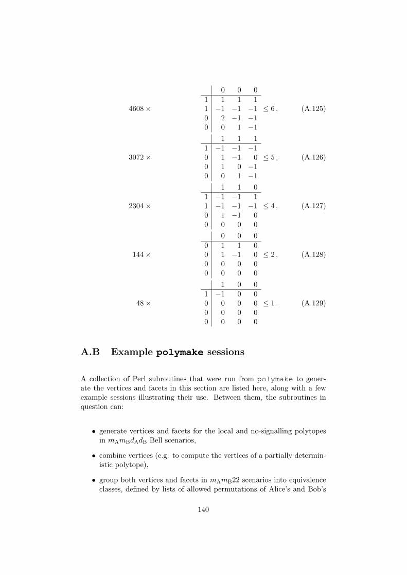
4608×
0 0 0
1 1 1 11 −1 −1 −10 2 −1 −10 0 1 −1
≤ 6 , (A.125)
3072×
1 1 1
1 −1 −1 −10 1 −1 00 1 0 −10 0 1 −1
≤ 5 , (A.126)
2304×
1 1 0
1 −1 −1 11 −1 −1 −10 1 −1 00 0 0 0
≤ 4 , (A.127)
144×
0 0 0
0 1 1 00 1 −1 00 0 0 00 0 0 0
≤ 2 , (A.128)
48×
1 0 0
1 −1 0 00 0 0 00 0 0 00 0 0 0
≤ 1 . (A.129)
A.B Example polymake sessions
A collection of Perl subroutines that were run from polymake to gener-ate the vertices and facets in this section are listed here, along with a fewexample sessions illustrating their use. Between them, the subroutines inquestion can:
• generate vertices and facets for the local and no-signalling polytopesin mAmBdAdB Bell scenarios,
• combine vertices (e.g. to compute the vertices of a partially determin-istic polytope),
• group both vertices and facets in mAmB22 scenarios into equivalenceclasses, defined by lists of allowed permutations of Alice’s and Bob’s
140

inputs (e.g.,{{A0}, {A1,A2}
}and
{{B0}, {B1,B2}
}).
• print and generate LATEX output for vertices and (for dichotomic out-puts) facets.
The code in question is not intended to be particularly elegant or efficient. Aworthwhile longer-term approach may be to incorporate some of the neededfunctionality described here into the faacets project [112, 113]. The re-mainder of this section gives a few example polymake sessions illustratingthe use of the subroutines.
The CHSH and positivity facets of L(2222) can be obtained, sorted intoequivalence classes, and printed out with the following sequence of com-mands:
polytope > $vL22 = vert_L_CG(2, 2, 2, 2) * prob_CGtoX(2, 2);polytope > $L22 = new Polytope(VERTICES=>$vL22);polytope > $fL22 = $L22->FACETS;polytope > $orbits = vec_classes_X($fL22, [[0, 1]], [[0, 1]]);polytope > $reps = fac_reps_X($orbits, 2, 2);polytope > print_ineqs_X($reps, 2, 2);
<A_0> + <B_0> - <A_0 B_0> <= 1
<A_0 B_0> + <A_0 B_1> + <A_1 B_0> - <A_1 B_1> <= 2
The following set of commands obtains and sorts the vertices of NS(2222)from its facets and prints out one of the PR boxes:
polytope > $fNS22 = fac_NS_CG(2, 2, 2, 2) * transpose(prob_XtoCG(2, 2));polytope > $NS22 = new Polytope(FACETS=>$fNS22);polytope > $vNS22 = $NS22->VERTICES;polytope > $orbits = vec_classes_X($vNS22, [[0, 1]], [[0, 1]]);polytope > $reps = prob_reps_X($orbits, 2, 2);polytope > $P = $reps * prob_XtoP(2, 2);polytope > print $P;1 1 0 1 0 0 0 0 0 1 0 1 0 0 0 0 01 1/2 0 1/2 0 0 1/2 0 1/2 1/2 0 0 1/2 0 1/2 1/2 0polytope > table_prob_P($P->row(1), 2, 2, 2, 2, "txt");+----------+----------+| 1/2 0 | 1/2 0 || 0 1/2 | 0 1/2 |+----------+----------+| 1/2 0 | 0 1/2 || 0 1/2 | 1/2 0 |+----------+----------+
The following example finds the facets of L(3322), composes the list of facetsof the intersection of DA0(3322) and DB0(3322), and displays one of the 1248vertices:
141

polytope > $vL33 = vert_L_CG(3, 3, 2, 2) * prob_CGtoX(3, 3);polytope > $fL33 = new Polytope(VERTICES=>$vL33)->FACETS;polytope > $orbits = vec_classes_X($fL33, [[0], [1, 2]], [[0], [1, 2]]);polytope > print fac_reps_X($orbits, 3, 3);...polytope > $f_ict = $orbits->[4] / $orbits->[5] / $orbits->[6] / $orbits
->[8] / $orbits->[9] / $orbits->[10] / $orbits->[11];polytope > $v_ict = new Polytope(FACETS=>$f_ict)->VERTICES;polytope > print $v_ict->rows;1248polytope > $orbits = vec_classes_X($v_ict, [[0], [1, 2]], [[0], [1, 2]]);polytope > $reps = prob_reps_X($orbits, 3, 3);polytope > table_prob_P($reps->[0] * prob_XtoP(3, 3), 3, 3, 2, 2, "txt");+----------+----------+----------+| 1/3 1/3 | 2/3 0 | 1/3 1/3 || 1/3 0 | 0 1/3 | 1/3 0 |+----------+----------+----------+| 2/3 0 | 1/3 1/3 | 1/3 1/3 || 0 1/3 | 1/3 0 | 1/3 0 |+----------+----------+----------+| 1/3 1/3 | 1/3 1/3 | 1/3 1/3 || 1/3 0 | 1/3 0 | 1/3 0 |+----------+----------+----------+
Finally, the following sequence sorts and prints LATEX source for the 932facets of the D1122(3322) polytope:
polytope > $vL11 = vert_L_CG(1, 1, 2, 2) * prob_CGtoX(1, 1);polytope > $fNS22 = fac_NS_CG(2, 2, 2, 2) * transpose(prob_XtoCG(2, 2));polytope > $vNS22 = new Polytope(FACETS=>$fNS22)->VERTICES;polytope > $vD33 = combine_all($vL11, $vNS22, 1, 1, 2, 2, 2, 2);polytope > $fD33 = new Polytope(VERTICES=>$vD33)->FACETS;polytope > print $fD33->rows;932polytope > $orbits = vec_classes_X($fD33, [[0], [1, 2]], [[0], [1, 2]]);polytope > $reps = fac_reps_X($orbits, 3, 3);polytope > table_ineqs_X($reps, 3, 3, "tex");\begin{array}{c|ccc}
& \phneg 1 & \phneg 1 & \phneg 0 \\ \hline\phneg 1 & - 1 & - 2 & \phneg 0 \\\phneg 1 & - 2 & \phneg 2 & \phneg 1 \\\phneg 0 & \phneg 0 & \phneg 1 & - 1 \\
\end{array} \leq 6...
(in the LATEX source for this document, \phneg is a macro defined by\newcommand{\phneg}{\phantom{-}}.)
142

Bibliography
[1] N. Gisin, G. Ribordy, W. Tittel, and H. Zbinden, Rev. Mod. Phys.74, 145 (2002).
[2] V. Scarani, H. Bechmann-Pasquinucci, N. J. Cerf, M. Dusek,N. Lutkenhaus, and M. Peev, Rev. Mod. Phys. 81, 1301 (2009).
[3] C. H. Bennett and G. Brassard, in Proceedings of IEEE InternationalConference on Computers, Systems and Signal Processing (IEEE, NewYork, 1984) pp. 175–179.
[4] I. Quantique, “Home,” http://www.idquantique.com/.[5] I. MagiQ Technologies, “Home,” http://www.magiqtech.com/
Home.html.[6] QuintessenceLabs Inc., “QuintessenceLabs Inc.” http:
//quintessencelabs.com/.[7] SeQureNet, “SeQureNet,” http://www.sequrenet.com/.[8] D. Stebila, M. Mosca, and N. Lutkenhaus, in Quantum Communi-
cation and Quantum Networking , Lecture Notes of the Institute forComputer Sciences, Social Informatics and Telecommunications Engi-neering, Vol. 36 (Springer, Berlin, Heidelberg, 2010) pp. 283–296.
[9] P. Shor, SIAM J. Comput. 26, 1484 (1997).[10] W. K. Wootters and W. H. Zurek, Nature 299, 802 (1982).[11] D. Dieks, Phys. Lett. A 92, 271 (1982).[12] F. Xu, B. Qi, and H.-K. Lo, New J. Phys. 12, 113026 (2010).[13] L. Lydersen, C. Wiechers, C. Wittmann, D. Elser, J. Skaar, and
V. Makarov, Nature Photon. 4, 686 (2010).[14] C. A. Fuchs, N. Gisin, R. B. Griffiths, C.-S. Niu, and A. Peres, Phys.
Rev. A 56, 1163 (1997).[15] H.-K. Lo, M. Curty, and K. Tamaki, Nature Photon. 8, 595 (2014).[16] M. A. Nielsen and I. L. Chuang, Quantum Computation and Quantum
Information (Cambridge University Press, 2000).[17] J. Preskill, “Lecture notes for physics 229: Quantum infor-
mation and computation,” http://www.theory.caltech.edu/people/preskill/ph229/ (1998), lecture notes.
[18] M. Christandl, “Quantum information theory,” http://www.itp.phys.ethz.ch/education/hs12/qsit (2012), lecture notes,
143

based on lecture notes by R. Renner.[19] E. Woodhead and S. Pironio, Phys. Rev. A 87, 032315 (2013).[20] Ø. Marøy, L. Lydersen, and J. Skaar, Phys. Rev. A 82, 032337 (2010).[21] B. Kraus, N. Gisin, and R. Renner, Phys. Rev. Lett 95, 080501 (2005).[22] E. Woodhead, Phys. Rev. A 88, 012331 (2013).[23] E. Woodhead, Phys. Rev. A 90, 022306 (2014).[24] D. Mayers and A. Yao, Quantum Inf. Comput. 4, 273 (2004).[25] A. Acın, N. Brunner, N. Gisin, S. Massar, S. Pironio, and V. Scarani,
Phys. Rev. Lett 98, 230501 (2007).[26] M. Paw lowski and N. Brunner, Phys. Rev. A 84, 010302(R) (2011).[27] E. Woodhead, C. C. W. Lim, and S. Pironio, in Theory of Quantum
Computation, Communication, and Cryptography , Lecture Notes inComputer Science, Vol. 7582 (Springer, Berlin, Heidelberg, 2013) pp.107–115.
[28] E. Woodhead and S. Pironio, “Secrecy in prepare-and-measure CHSHgames with a qubit bound,” Article in preparation.
[29] E. Woodhead, J. Silman, and S. Pironio, “Partially deterministicpolytopes,” Article in preparation.
[30] C. H. Bennett, G. Brassard, and J.-M. Robert, SIAM J. Comput. 17,210 (1988).
[31] I. Devetak and A. Winter, Proc. R. Soc. A 461, 207 (2005).[32] R. Renner, N. Gisin, and B. Kraus, Phys. Rev. A 72, 012332 (2005).[33] R. Renner, Security of Quantum Key Distribution, Ph.D. thesis, ETH
Zurich (2005), arXiv:quant-ph/0512258 .[34] I. Csiszar and J. Korner, IEEE Trans. Inf. Th. 24, 339 (1978).[35] H.-K. Lo, H. F. Chau, and M. Ardehali, J. Cryptology 18, 133 (2005).[36] B. Huttner, N. Imoto, N. Gisin, and T. Mor, Phys. Rev. A 51, 1863
(1995).[37] G. Brassard, N. Lutkenhaus, T. Mor, and B. C. Sanders, Phys. Rev.
Lett 85, 1330 (2000).[38] W.-Y. Hwang, Phys. Rev. Lett 91, 057901 (2003).[39] H.-K. Lo, X. Ma, and K. Chen, Phys. Rev. Lett 94, 230504 (2005).[40] C. H. Bennett, G. Brassard, and N. D. Mermin, Phys. Rev. Lett 68,
557 (1992).[41] A. K. Ekert, Phys. Rev. Lett 67, 661 (1991).[42] M. Koashi and J. Preskill, Phys. Rev. Lett 90, 057902 (2003).[43] C. H. Bennett, Phys. Rev. Lett 68, 3121 (1992).[44] D. Bruß, Phys. Rev. Lett 81, 3018 (1998).[45] H. Bechmann-Pasquinucci and N. Gisin, Phys. Rev. A 59, 4238 (1999).[46] V. Scarani, A. Acın, G. Ribordy, and N. Gisin, Phys. Rev. Lett 92,
057901 (2004).[47] H.-K. Lo, M. Curty, and B. Qi, Phys. Rev. Lett 108, 130503 (2012).[48] B. Huttner and A. K. Ekert, J. Mod. Opt. 41, 2455 (1994).[49] M. Tomamichel, C. C. W. Lim, N. Gisin, and R. Renner, Nat. Com-
144

mun. 3, 634 (2012).[50] M. Ben-Or, M. Horodecki, D. W. Leung, D. Mayers, and J. Oppen-
heim, in Theory of Cryptography , Lecture Notes in Computer Science,Vol. 3378, edited by J. Kilian (Springer, Berlin, Heidelberg, 2005) pp.386–406.
[51] R. Renner and R. Konig, in Theory of Cryptography , Lecture Notesin Computer Science, Vol. 3378, edited by J. Kilian (Springer, Berlin,Heidelberg, 2005) pp. 407–425.
[52] V. Scarani and C. Kurtsiefer, “The black paper of quantum cryp-tography: real implementation problems,” (2009), arXiv:0906.4547[quant-ph] .
[53] P. W. Shor and J. Preskill, Phys. Rev. Lett 85, 441 (2000).[54] G. Smith, J. M. Renes, and J. A. Smolin, Phys. Rev. Lett 100, 170502
(2008).[55] J. Bae and A. Acın, Phys. Rev. A 75, 012334 (2007).[56] M. Mertz, H. Kampermann, Z. Shadman, and D. Bruß, Phys. Rev.
A 87, 042312 (2013).[57] F. Xu, S. Sajeed, S. Kaiser, Z. Tang, L. Qian, V. Makarov,
and H.-K. Lo, “Experimental quantum key distribution with sourceflaws and tight finite-key analysis,” (2014), QCrypt 2014 presen-tation slides available via http://2014.qcrypt.net/program/,arXiv:1408.3667 [quant-ph] .
[58] D. Mayers and A. Yao, in Proceedings of the 39th Annual Symposiumon Foundations of Computer Science (IEEE Computer Society, LosAlamitos, 1998) pp. 503–509.
[59] M. Berta, M. Christandl, R. Colbeck, J. M. Renes, and R. Renner,Nature Phys. 6, 659 (2010).
[60] M. Tomamichel and R. Renner, Phys. Rev. Lett 106, 110506 (2011).[61] D. Gottesman, H.-K. Lo, N. Lutkenhaus, and J. Preskill, Quantum
Inf. Comput. 4, 325 (2004).[62] M. Koashi, New J. Phys. 11, 045018 (2009).[63] E. Biham, M. Boyer, G. Brassard, J. van de Graaf, and T. Mor,
Algorithmica 34, 372 (2002).[64] J. M. Renes and J.-C. Boileau, Phys. Rev. Lett 103, 020402 (2009).[65] D. Mayers, J. ACM 48, 351 (2001).[66] R. Renner, Nature Phys. 3, 645 (2007).[67] M. Christandl, R. Konig, and R. Renner, Phys. Rev. Lett 102, 020504
(2009).[68] C. W. Helstrom, Quantum detection and estimation theory (Academic
Press, New York, 1976).[69] R. Jozsa, J. Mod. Opt. 41, 2315 (1994).[70] C. A. Fuchs and J. van de Graaf, IEEE Trans. Inf. Th. 45, 1216 (1999).[71] L. Mirsky, Monatsh. Math. 79, 303 (1975).[72] J.-D. Bancal, N. Gisin, Y.-C. Liang, and S. Pironio, Phys. Rev. Lett
145

106, 250404 (2011).[73] D. Rosset, R. Ferretti-Schobitz, J.-D. Bancal, N. Gisin, and Y.-C.
Liang, Phys. Rev. A 86, 062325 (2012).[74] N. Gisin, (2011), private communication.[75] E. H. Lieb and M. B. Ruskai, J. Math. Phys. 14, 1938 (1973).[76] W. Roga, M. Fannes, and K. Zyczkowski, Phys. Rev. Lett 105, 040505
(2010).[77] R. Konig, R. Renner, and C. Schaffner, IEEE Trans. Inf. Th. 55, 4337
(2009).[78] M. Tomamichel, A Framework for Non-Asymptotic Quantum Infor-
mation Theory, Ph.D. thesis, ETH Zurich (2012), arXiv:1203.2142[quant-ph] .
[79] J. F. Clauser, M. A. Horne, A. Shimony, and R. A. Holt, Phys. Rev.Lett 23, 880 (1969).
[80] C. C. W. Lim, C. Portmann, M. Tomamichel, R. Renner, andN. Gisin, Phys. Rev. X 3, 031006 (2013).
[81] B. S. Cirel’son, Lett. Math. Phys. 4, 93 (1980).[82] L. A. Khalfin and B. S. Tsirelson, in Symposium on the Foundations
of Modern Physics (World Scientific, Singapore, 1985) pp. 441–460.[83] L. J. Landau, Phys. Lett. A 120, 54 (1987).[84] L. Masanes, S. Pironio, and A. Acın, Nat. Commun. 2, 238 (2011).[85] S. Pironio, A. Acın, S. Massar, A. Boyer de La Giroday, D. N. Mat-
sukevich, P. Maunz, S. Olmschenk, D. Hayes, L. Luo, T. A. Manning,and C. Monroe, Nature 464, 1021 (2010).
[86] C. Jordan, Bull. Soc. Math. Fr. 3, 103 (1875).[87] S. Pironio, A. Acın, N. Brunner, N. Gisin, S. Massar, and V. Scarani,
New J. Phys. 11, 045021 (2009).[88] T. Lunghi, J. Bohr Brask, C. C. W. Lim, Q. Lavigne, J. Bowles,
A. Martin, H. Zbinden, and N. Brunner, “A self-testing quantumrandom number generator,” (2014), arXiv:1410.2790 [quant-ph] .
[89] C. Branciard, E. G. Cavalcanti, S. P. Walborn, V. Scarani, and H. M.Wiseman, Phys. Rev. A 85, 010301 (2012).
[90] M. Tomamichel, F. Fehr, J. Kaniewski, and S. Wehner, New J. Phys.15, 103002 (2013).
[91] N. Brunner, D. Cavalcanti, S. Pironio, V. Scarani, and S. Wehner,Rev. Mod. Phys. 86, 419 (2014).
[92] J. S. Bell, Physics 1, 195 (1964).[93] P. Rastall, Found. Phys. 15, 963 (1985).[94] S. Popescu and D. Rohrlich, Found. Phys. 24, 379 (1994).[95] J. S. Bell, The theory of local beables, Ref.TH.2053-CERN (CERN,
1975).[96] T. Norsen, Am. J. Phys. 79, 1261 (2011).[97] A. Einstein, B. Podolsky, and N. Rosen, Phys. Rev. 47, 777 (1935).[98] J. Barrett, L. Hardy, and A. Kent, Phys. Rev. Lett 95, 010503 (2005).
146

[99] A. Acın, S. Massar, and S. Pironio, New J. Phys. 8, 126 (2006).[100] O. Nieto Silleras, S. Pironio, and J. Silman, New J. Phys. 16, 013035
(2014).[101] J.-D. Bancal, L. Sheridan, and V. Scarani, New J. Phys. 16, 033011
(2014).[102] M. Navascues, S. Pironio, and A. Acın, Phys. Rev. Lett 98, 010401
(2007).[103] M. Navascues, S. Pironio, and A. Acın, New J. Phys. 10, 073013
(2008).[104] M. Navascues, S. Pironio, and A. Acın, in Handbook on Semidefi-
nite, Conic and Polynomial Optimization, International Series in Op-erations Research & Management Science, Vol. 166, edited by M. F.Anjos and J. B. Lasserre (Springer US, 2012) pp. 601–634.
[105] I. Pitowsky, Math. Prog. 50, 395 (1991).[106] D. Collins and N. Gisin, J. Phys. A: Math. Gen. 37, 1775 (2004).[107] A. Fine, Phys. Rev. Lett 48, 291 (1982).[108] J. F. Clauser and M. A. Horne, Phys. Rev. D 10, 526 (1974).[109] E. Gawrilow and M. Joswig, in Polytopes — Combinatorics and Com-
putation, DMV Seminar, Vol. 29, edited by G. Kalai and G. M. Ziegler(Birkhauser, 2000) pp. 43–74.
[110] K. Fukuda, “cdd and cddplus Homepage,” http://www.inf.ethz.ch/personal/fukudak/cdd_home/cdd.html.
[111] M. Froissart, Nuovo Cimento B 64, 241 (1981).[112] D. Rosset, J.-D. Bancal, and N. Gisin, J. Phys. A: Math. Theor. 47,
424022 (2014).[113] J.-D. Bancal and D. Rosset, “Faacets - Faacets.com,” http://www.
faacets.com/, source code available at https://github.com/denisrosset/faacets.
147