imperial college of science, technology & medicine

Imperial College of Science, Technology & Medicine

University of London

Exploiting the Laser Scanning Facility for VibrationMeasurements

Milena Martarelli

A thesis submitted to the University of Londonfor the degree of Doctor of Philosophy

May 2001

I

Abstract

The aim of this research was to explore a vibration measurement technique

based on the use of a non-contacting response transducer which can be set

continuously scanning over the surface of a sinusoidally-excited structure.

Specifically in this context, a laser Doppler vibrometer (LDV) was employed as

a remote velocity transducer so that the specific testing technique studies was

classified as continuous scanning laser Doppler vibrometry (CSLDV).

This technique is a type of “spatial field” measurement (such as is holography)

that aims to overtake the essential limitation of conventional vibration tests, i.e.

the number of measured points is limited by the set of transducers that can be

physically attached to the structure so that the spatial resolution of mode

shapes derived from such measurements is limited. By using an optical non-

contacting transducer which scans continuously across the area under test,

vibration information can be derived at each point of the scanned pattern

without any physical restriction.

II

Basically, the work is divided into two main sections. The first section presents

an introduction to laser vibrometry, while the second concentrates on both

theoretical and practical aspects of the CSLDV method.

When an LDV is scanned continuously along an arbitrarily line, the LDV output

is an amplitude-modulated sine wave according to the structure operational

deflection shape (combination of mode shapes). Smooth mode shapes, which

can be defined by polynomial functions across the scanned area, may be

recovered as a set of polynomial coefficients derived from the LDV output

analysed in the frequency domain, which spectrum comprises sidebands

centred on the excitation frequency and spaced at multiples of the scan

frequency(ies). When the extent of the scanned line reduces until it becomes

shorter than the wavelength of the vibration pattern, the number of sidebands

decreases to a single pair only, from which angular and translational vibration

responses at the point addressed can be recovered.

The methodical approach of the research investigation consisted of a theoretical

analysis of the continuous scanning technique, the numerical simulation

(virtual testing) and the experimental validation on simple experimental

models. Software for control, data-acquisition and post-processing was

developed in order to build a user-friendly laboratory tool to apply the CSLDV

in all its facets. Finally, the techniques were shown to work successfully in

practical test conditions, by applying them to complex structures taken from

industrial case studies.

III

Acknowledgements

I wish to express my gratitude to my supervisor Professor D. J. Ewins for his

interest in this project, his strategic guidance concerning the scientific

development of this work and for his philosophical suggestions during the

writing up of this thesis.

Special thanks are due to Mr A. B. Stanbridge for his fundamental teaching and

useful discussion throughout the duration of this research. I would like to thank

also my former colleagues Drs Götz Von Groll and Saeed Ziaei-Rad for their

friendship over the years and their scientific and technical assistance in solving

practical problems.

I thank the entire Dynamics group for the cooperation and the encouraging

support during my stay at Imperial College, especially Ms Liz Savage for her

help and friendly advise.

I acknowledge the financial support of the BRITE/EURAM VALSE project

which entirely funded this research. I would like to thank all the partners

involved in the project and, in particular, Dr Paolo Castellini, Professors E. P.

Tomasini and N. Paone from University of Ancona, Dr Karl Bendel from Bosch,

Dr David Storer from CRF and Dr Fernando Baldoni from

Bridgestone/Firestone.

IV

Contents

List of Figures XI

List f Tables XXVII

1. Introduction 1

1.1. Background . . . . . . . . . . . . . . . . . . . . . . . . . . . . . . . . . . . . . . . . . . . . 1

1.2. Test Requirements for Advanced Applications . . . . . . . . . . . . . . 3

1.2.1 Introduction . . . . . . . . . . . . . . . . . . . . . . . . . . . . . . . . . . . . 3

1.2.2 Need for Non –Contact Measurement Devices . . . . . . 4

1.2.3 Need for Spatially–Dense Measurements . . . . . . . . . . . 4

1.2.4 Need for Continuous–Field Measurements . . . . . . . . . 6

1.2.5 Need for Multiple DOFs Measurements . . . . . . . . . . . . 6

1.3. Objectives of Research Project . . . . . . . . . . . . . . . . . . . . . . . . . . . . 7

1.4. Literature Review . . . . . . . . . . . . . . . . . . . . . . . . . . . . . . . . . . . . . . . 8

1.5. Structure of Thesis . . . . . . . . . . . . . . . . . . . . . . . . . . . . . . . . . . . . . . . 8

2. LDV Theory 12

2.1. Introduction . . . . . . . . . . . . . . . . . . . . . . . . . . . . . . . . . . . . . . . . . . . . 12

V

2.2. Doppler Effect . . . . . . . . . . . . . . . . . . . . . . . . . . . . . . . . . . . . . . . . . . 15

2.2.1 Introduction . . . . . . . . . . . . . . . . . . . . . . . . . . . . . . . . . . . . 15

2.2.2 Stationary Source - Moving Observer . . . . . . . . . . . . . . 15

2.2.3 Moving Source - Stationary Observer . . . . . . . . . . . . . . 16

2.2.4 Scattering Condition . . . . . . . . . . . . . . . . . . . . . . . . . . . . . 16

2.3. Laser Light . . . . . . . . . . . . . . . . . . . . . . . . . . . . . . . . . . . . . . . . . . . . . 19

2.4. Laser Speckle . . . . . . . . . . . . . . . . . . . . . . . . . . . . . . . . . . . . . . . . . . . 23

2.5. Frequency Broadening related to the Laser Speckle . . . . . . . . . . 31

2.6. Michelson’s Interferometer . . . . . . . . . . . . . . . . . . . . . . . . . . . . . . . 47

2.7. Mach-Zender Interferometer . . . . . . . . . . . . . . . . . . . . . . . . . . . . . . 50

2.8. Velocity direction investigation . . . . . . . . . . . . . . . . . . . . . . . . . . . 52

2.9. Polytec Laser Doppler Vibrometer . . . . . . . . . . . . . . . . . . . . . . . . 58

2.10. Ometron Laser Doppler Vibrometer . . . . . . . . . . . . . . . . . . . . . . . 63

2.11. Conclusions . . . . . . . . . . . . . . . . . . . . . . . . . . . . . . . . . . . . . . . . . . . . 70

3. SLDV Theory 72

3.1. Introduction . . . . . . . . . . . . . . . . . . . . . . . . . . . . . . . . . . . . . . . . . . . . 72

3.2. Basics of SLDV Technology . . . . . . . . . . . . . . . . . . . . . . . . . . . . . . . 74

3.3. Scanning Mirror System . . . . . . . . . . . . . . . . . . . . . . . . . . . . . . . . . . 75

3.4. Polytec Discrete Scanning Utility . . . . . . . . . . . . . . . . . . . . . . . . . . 79

3.5. Speckle Noise and its Improvement by the Exploitation of

Commercial Devices (Tracking filter and Signal Enhancement

Facility) . . . . . . . . . . . . . . . . . . . . . . . . . . . . . . . . . . . . . . . . . . . . . . . . 79

3.6. Vibration Measurements By Discrete Scanning . . . . . . . . . . . . . . 81

3.7. Fast Scan Option . . . . . . . . . . . . . . . . . . . . . . . . . . . . . . . . . . . . . . . . 89

3.8. Conclusions. . . . . . . . . . . . . . . . . . . . . . . . . . . . . . . . . . . . . . . . . . . . . 90

VI

4. Continuous Scanning Technique Applied on MDOF Vibration

Response Measurements 92

4.1. Measurement Methodology. . . . . . . . . . . . . . . . . . . . . . . . . . . . . . 92

4.2. Analysis of Linear Scan and Experimental Validation . . . . . . . . 100

4.3. Analysis of Circular Scan and Experimental Validation . . . . . . . 105

4.4. Analysis of Conical Scan and Experimental Validation . . . . . . . 109

4.5. Analysis of Conical –Circular Scan and Experimental Validation 124

4.6. Calibration of Continous Scanning Techniques . . . . . . . . . . . . . . 136

4.6.1 Mirror Calibration . . . . . . . . . . . . . . . . . . . . . . . . . . . . . . . 136

4.6.2 Line-Scan Calibration . . . . . . . . . . . . . . . . . . . . . . . . . . . . 142

4.6.3 Circular-Scan Calibration . . . . . . . . . . . . . . . . . . . . . . . . . 144

4.6.4 Conical-Scan Calibration . . . . . . . . . . . . . . . . . . . . . . . . . 145

4.7. Conclusions . . . . . . . . . . . . . . . . . . . . . . . . . . . . . . . . . . . . . . . . . . . . 146

5. Continuous Scanning Technique Applied to Operational Deflection

Shape Measurements 147

5.1. Introduction . . . . . . . . . . . . . . . . . . . . . . . . . . . . . . . . . . . . . . . . . . . . 147

5.2. Measurement Methodology . . . . . . . . . . . . . . . . . . . . . . . . . . . . . . 149

5.3. Analysis of Linear Scan . . . . . . . . . . . . . . . . . . . . . . . . . . . . . . . . . . 151

5.3.1 Introduction . . . . . . . . . . . . . . . . . . . . . . . . . . . . . . . . . . . . 151

5.3.2 Uniform Straight-Line Scan . . . . . . . . . . . . . . . . . . . . . . . 151

5.3.2.1 Numerical Simulation . . . . . . . . . . . . . . . . . . . . 151

5.3.2.2 Experimental Validation . . . . . . . . . . . . . . . . . . 156

5.3.3 Sinusoidal Straight-Line Scan . . . . . . . . . . . . . . . . . . . . . 161

5.3.3.1 Mathematical Investigation. . . . . . . . . . . . . . . 161

5.3.3.2 Numerical Simulation . . . . . . . . . . . . . . . . . . . 165

VII

5.3.3.2.1 Real Vibration Response. . . . . . . . . . . . . . 165

5.3.3.2.2 Complex Vibration Response. . . . . . . . . . 169

5.3.3.2.3 Mirror Delay Effect Investigation . . . . . . 173

5.3.3.3 Experimental Validation . . . . . . . . . . . . . . . . . 177

5.3.3.4 Experimental Investigation using the Point-by-

Point Technique . . . . . . . . . . . . . . . . . . . . . . . . . 181

5.4. Analysis of Circular Scan . . . . . . . . . . . . . . . . . . . . . . . . . . . . . . . . . 184

5.4.1 Introduction . . . . . . . . . . . . . . . . . . . . . . . . . . . . . . . . . . . . 184

5.4.2 Mathematical Investigation . . . . . . . . . . . . . . . . . . . . . . . 185

5.4.3 Numerical Simulation on a Rectangular Plate . . . . . . . 187

5.4.4 Numerical Simulation on a Disc . . . . . . . . . . . . . . . . . . . 191

5.4.5 Experimental Investigtion on a Disc . . . . . . . . . . . . . . . 195

5.5. Analysis of Area Scan and Experimental Validation . . . . . . . . . 204

5.5.1 Introduction . . . . . . . . . . . . . . . . . . . . . . . . . . . . . . . . . . . . 204

5.5.2 Two-Dimensional Uniform Scan. . . . . . . . . . . . . . . . . . . 207

5.5.3 Sinusoidal Parallel Stright-Line Scans . . . . . . . . . . . . . . 209

5.5.4 Two-Dimensional Sinusoidal Scan . . . . . . . . . . . . . . . . . 210


5.5.4.2 Numerical Simulation . . . . . . . . . . . . . . . . . . . 214

5.5.4.2.1 Real Vibration Response. . . . . . . . . . . . . . 214

5.5.4.2.2 Complex Vibration Response. . . . . . . . . . 223

5.5.4.2.3 Mirror Delay Effect Investigation . . . . . . . 226


5.5.4.3.1 Experimental Set-upDescription. . . . . . . . 232

5.5.4.3.2 Test on the Plate at the Fourth Resonance . 234

VIII

5.5.4.3.3 Test on the Plate at the Fifth Resonance. . 242

5.5.5 Sinusoidal Scan on a Circular Area . . . . . . . . . . . . . . . . . 244


5.5.5.2 Numerical Simulation . . . . . . . . . . . . . . . . . . . . 248


5.6. Modal Analysis of ODSs derived by Area Scan . . . . . . . . . . . . . . 260

5.6.1 Introduction . . . . . . . . . . . . . . . . . . . . . . . . . . . . . . . . . . . . 260

5.6.2 Experimental Modal Analysis on the Garteur Structure 261

5.6.3 Concluding Remarks. . . . . . . . . . . . . . . . . . . . . . . . . . . . . 281

5.7. Conclusions . . . . . . . . . . . . . . . . . . . . . . . . . . . . . . . . . . . . . . . . . . . . 283

6. Virtual Testing 285

6.1. Introduction . . . . . . . . . . . . . . . . . . . . . . . . . . . . . . . . . . . . . . . . . . . . 285

6.2. Virtual Testing Technique . . . . . . . . . . . . . . . . . . . . . . . . . . . . . . . . . 286

6.3. Mathematical Model . . . . . . . . . . . . . . . . . . . . . . . . . . . . . . . . . . . . . 287

6.4. Speckle Model. . . . . . . . . . . . . . . . . . . . . . . . . . . . . . . . . . . . . . . . . . . 290

6.4.1 Introduction. . . . . . . . . . . . . . . . . . . . . . . . . . . . . . . . . . . . . 290

6.4.2 Theoretical Model of the Light Intensity Collected by the

Photodetector . . . . . . . . . . . . . . . . . . . . . . . . . . . . . . . . . . . 292

6.4.3 Experimental Speckle Noise Analysis . . . . . . . . . . . . . . 296

6.4.4 Simulated Speckle Noise . . . . . . . . . . . . . . . . . . . . . . . . . 303

6.5. Experiment Simulation by using the Model developed and

Comparison with the Real Measurement Data . . . . . . . . . . . . . . . 307

6.6. Averaging Procedure . . . . . . . . . . . . . . . . . . . . . . . . . . . . . . . . . . . . 311

6.7. Conclusions. . . . . . . . . . . . . . . . . . . . . . . . . . . . . . . . . . . . . . . . . . . . . 317

IX

7. Application of the Continuous Scanning Technique in Industrial

Cases 319

7.1 Introduction . . . . . . . . . . . . . . . . . . . . . . . . . . . . . . . . . . . . . . . . . . 319

7.2 Short-Line and Small-Circular Scanning Techniques Applied to

Practical Cases (RDOF or Angular Motion Measurement) . . . 320

7.2.1 Experimental Set-up Description . . . . . . . . . . . . . . . . . . 320

7.2.2 Test of the “1203” Structure . . . . . . . . . . . . . . . . . . . . . . . 324

7.2.3 Test of the “breadboard” Structure . . . . . . . . . . . . . . . . . 326

7.3 One-Dimensional Long - Scan Technique Application in Practical

Cases . . . . . . . . . . . . . . . . . . . . . . . . . . . . . . . . . . . . . . . . . . . . . . . . 337

7.3.1 Experimental Set-up Description . . . . . . . . . . . . . . . . . . 337

7.3.2 Uniform-Rate Straight-Line Scan on the IVECO DAILY

Rear Panel . . . . . . . . . . . . . . . . . . . . . . . . . . . . . . . . . . . . . . 339

7.3.3 Sinusoidal Straight-Line Scan on the IVECO DAILY Rear

Panel . . . . . . . . . . . . . . . . . . . . . . . . . . . . . . . . . . . . . . . . . . 347

7.3.4 Parallel Sinusoidal Straight-Line Scan on the FIAT PUNTO

Windscreen . . . . . . . . . . . . . . . . . . . . . . . . . . . . . . . . . . . . . 351

7.4 Two-Dimensional Long - Scan Technique Application to Practical

Cases . . . . . . . . . . . . . . . . . . . . . . . . . . . . . . . . . . . . . . . . . . . . . . . 355

8.2.1 Introduction . . . . . . . . . . . . . . . . . . . . . . . . . . . . . . . . . . . . 355

8.2.2 Two-dimensional Uniform-Rate Scan . . . . . . . . . . . . . . 356

8.2.3 Sinusoidal Two-dimensional Scan on the Rear Panel of the

IVECO Lorry Cab . . . . . . . . . . . . . . . . . . . . . . . . . . . . . . . 358

7.4 Conclusions. . . . . . . . . . . . . . . . . . . . . . . . . . . . . . . . . . . . . . . . . . . 364

8. Conclusions and Suggestion for Further Work 366

8.1. Overall Conclusions . . . . . . . . . . . . . . . . . . . . . . . . . . . . . . . . . . . . . 366

X

8.2. Summary of the Major Conclusions . . . . . . . . . . . . . . . . . . . . . . . 367

8.2.1 Development of the CLSDV Techniques for MDOF

Vibration Response and ODS Measurements. . . . . . . . 367

8.2.2 Simulation of the CLSDV Techniques. . . . . . . . . . . . . . 369

8.2.3 Experimental Validation of the CLSDV Techniques. . 370

8.2.4 Application of the CLSDV Techniques in Industrial Case

Studies . . . . . . . . . . . . . . . . . . . . . . . . . . . . . . . . . . . . . . . . . 371

8.3. Suggestions for Further Work. . . . . . . . . . . . . . . . . . . . . . . . . . . . . 372

9. References 373

Appendix i

A.1. LabVIEW Programs . . . . . . . . . . . . . . . . . . . . . . . . . . . . . . . . . . . . . i

A.1.1 Shaker Control . . . . . . . . . . . . . . . . . . . . . . . . . . . . . . . . . . i

A.1.2 Mirror Driver Control – Case of Scans at Uniform Rate ii

A.1.3 Acquisition Control . . . . . . . . . . . . . . . . . . . . . . . . . . . . . . iii

A.1.4 Demodulation Program . . . . . . . . . . . . . . . . . . . . . . . . . . . iv

A.1.5 Mirror Driver Control – Case of Sinusoidal Scans . . . . v

A.1.6 Spectrum Analyser Program . . . . . . . . . . . . . . . . . . . . . . vi

A.1.7 ODS Recovery Program . . . . . . . . . . . . . . . . . . . . . . . . . . vii

A.1.8 Automatic Shaker Control and Acquisition Control for

Step-Sine Tests . . . . . . . . . . . . . . . . . . . . . . . . . . . . . . . . . . ix

A.2. Measured FRF data from CSLDV Techniques.. . . . . . . . . . . . . . . xi

XI

List of Figures

1.1 Virtual transducers location along the laser beam scan line . . . . 5

2.1 Basic LDV arrangement . . . . . . . . . . . . . . . . . . . . . . . . . . . . . . . . . . . 13

2.2 Doppler effect (Stationary Source-Moving Observer) . . . . . . . . . 16

2.3 Doppler effect (Scattering Condition) . . . . . . . . . . . . . . . . . . . . . . . 17

2.4 Electric field fluctuation along its direction of propagation . . . . 20

2.5 Gaussian light beam profile . . . . . . . . . . . . . . . . . . . . . . . . . . . . . . . 22

2.6 Light scattering and light collection process . . . . . . . . . . . . . . . . . 25

2.7 Velocity Drop out . . . . . . . . . . . . . . . . . . . . . . . . . . . . . . . . . . . . . . . . . 29

2.8 Schematic of the laser optical path . . . . . . . . . . . . . . . . . . . . . . . . . 32

2.9 Gaussian function behavior varying the parameter w . . . . . . . . . . 39

2.10 Bessel function behavior depending on the factor γ0 . . . . . . . . . . . 40

2.11 Gaussian and Bessel functions in the first case study . . . . . . . . . . 41

2.12 Product of f1 and f2 for the first case study . . . . . . . . . . . . . . . . . . . 42

2.13 Gaussian and Bessel functions in the second case study . . . . . . . . 42

2.14 Product of f1 and f2 for the second case study . . . . . . . . . . . . . . . . . 43

2.15 Averaged power spectrum components for the two cases study . 44

2.16 Schematic representation of Michelson’s interferometer . . . . . . 48

XII

2.17 Schematic representation of Mach-Zehnder interferometer . . . . 51

2.18 Plot of the output signal from the first detector (blue) and the

output signals from the second detector (green) being fD

positive in the first picture and negative in the second one . 53

2.19 Schematic of the optical light split and phase shift between the

two channels and the mixing of the two outputs after a second

phase shift . 55

2.20 Frequency shifting and time-resolved velocity, [33] . . . . . . . . . . . 57

2.21 Polytec LDV arrangement . . . . . . . . . . . . . . . . . . . . . . . . . . . . . . . . 59

2.22 Quarter wave plate working principle . . . . . . . . . . . . . . . . . . . . . . . 61

2.23 Ometron VPI configuration . . . . . . . . . . . . . . . . . . . . . . . . . . . . . . . 64

2.24 Doppler signals at the two detectors being the target velocity

positive (first) and negative (second) . 68

2.25 Intensity output for positive (green) and negative (red) target

velocity . 69

3.1 Schematic representation of the mirrors rotation . . . . . . . . . . . . . . 76

3.2 Flow-chart of the feedback control action . . . . . . . . . . . . . . . . . . . 77

3.3 Experimental configuration . . . . . . . . . . . . . . . . . . . . . . . . . . . . . . . 82

3.4 Measurement points grid . . . . . . . . . . . . . . . . . . . . . . . . . . . . . . . . . . 82

3.5 Transfer mobility at point A . . . . . . . . . . . . . . . . . . . . . . . . . . . . . . . 85

3.6 ODS at 181.9 Hz . . . . . . . . . . . . . . . . . . . . . . . . . . . . . . . . . . . . . . . . . . 86

3.7 ODS at 239.1 Hz . . . . . . . . . . . . . . . . . . . . . . . . . . . . . . . . . . . . . . . . . 86

3.8 ODS at 181.9 Hz (4th Mode). . . . . . . . . . . . . . . . . . . . . . . . . . . . . . . . 87

3.9 ODS at 239.1 Hz (5th Mode). . . . . . . . . . . . . . . . . . . . . . . . . . . . . . . . 88

3.10 Measured and theoretical ODSs overlaid for mode 4th (left) and

mode 5th (right). . 88

3.11 ODS at 181.9 Hz . . . . . . . . . . . . . . . . . . . . . . . . . . . . . . . . . . . . . . . . . . 90

3.12 ODS at 239.1 Hz . . . . . . . . . . . . . . . . . . . . . . . . . . . . . . . . . . . . . . . . . . 90

4.1 Vibration decomposition in the cartesian system of coordinates . 94

4.2 Circular-Conical scan . . . . . . . . . . . . . . . . . . . . . . . . . . . . . . . . . . . . . 96

XIII

4.3 Mirror’s driver signals . . . . . . . . . . . . . . . . . . . . . . . . . . . . . . . . . . . . 97

4.4 Circular scan configuration . . . . . . . . . . . . . . . . . . . . . . . . . . . . . . . . 97

4.5 Schematic of the tested structure and the measurement

equipment . 99

4.6 Laser beam scan and vibration DOFs associated to the surface . . 100

4.7 Linear scan set up . . . . . . . . . . . . . . . . . . . . . . . . . . . . . . . . . . . . . . . . 103

4.8 LDV output and Mirror Drive Signal plotted together . . . . . . . . . 104

4.9 Circular scan configuration . . . . . . . . . . . . . . . . . . . . . . . . . . . . . . . . 106

4.10 Circular scan set up . . . . . . . . . . . . . . . . . . . . . . . . . . . . . . . . . . . . . . 108

4.11 Conical scan configuration . . . . . . . . . . . . . . . . . . . . . . . . . . . . . . . . 110

4.12 Conical scan set up . . . . . . . . . . . . . . . . . . . . . . . . . . . . . . . . . . . . . . . . 112

4.13 Lens deviation angle . . . . . . . . . . . . . . . . . . . . . . . . . . . . . . . . . . . . . 112

4.14 Cylindrical representation of vibration vector . . . . . . . . . . . . . . . . 114

4.15 Accelerometer/Shaker set-up for Conical Scan trial . . . . . . . . . . . 119

4.16 Vibration velocity amplitude measured with a conical scan

LDV and an accelerometer . 120

4.17 Conical scan set-up on the beam . . . . . . . . . . . . . . . . . . . . . . . . . . . . 121

4.18 Accuracy of Vibration Direction measured by Conical Scan . . . . 122

4.19 Noise floor outline . . . . . . . . . . . . . . . . . . . . . . . . . . . . . . . . . . . . . . . . 123

4.20 Conical-circular scan configuration . . . . . . . . . . . . . . . . . . . . . . . . . 125

4.21 Inside-focus conical-circular scan . . . . . . . . . . . . . . . . . . . . . . . . . . . 126

4.22 Outside-focus conical-circular scan . . . . . . . . . . . . . . . . . . . . . . . . . 129

4.23 Conical-circular scan degeneration for Φ going to zero . . . . . . . . 130

4.24 Conical-Circular scan set-up . . . . . . . . . . . . . . . . . . . . . . . . . . . . . . . 132

4.25 Single point measurements configuration . . . . . . . . . . . . . . . . . . . 133

4.26 LDV output signal before and after applying the mirror delay

correction . 138

4.27 Phase angles and relative time shifts plotted against the scan

frequency . 140

4.28 Phase angles and relative time shifts plotted against the scan

frequency . 141

XIV

4.29 Comparison of phase angles associated to the delay of both the

mirrors . 142

4.30 Conical scan configuration . . . . . . . . . . . . . . . . . . . . . . . . . . . . . . . . 145

5.1 Laser linear scan on the beam . . . . . . . . . . . . . . . . . . . . . . . . . . . . . . 152

5.2 Second mode deflection shape . . . . . . . . . . . . . . . . . . . . . . . . . . . . . 154

5.3 LDV output modulated by the bending mode shape of the

beam (red line) . 155

5.4 LDV output signal (blue) and mirror driving signal (red) . . . . . 157

5.5 In-phase and out-of-phase components of the ODS at 58 Hz . . . 158



5.8 Analytical mode shape and ODS at 58 Hz . . . . . . . . . . . . . . . . . . . 160

5.9 Analytical mode shape and ODS at 311 Hz . . . . . . . . . . . . . . . . . . 160

5.10 Analytical mode shape and ODS at 766 Hz . . . . . . . . . . . . . . . . . . 160

5.11 Vibration pattern at different time instants . . . . . . . . . . . . . . . . . . 166

5.12 Velocity response . . . . . . . . . . . . . . . . . . . . . . . . . . . . . . . . . . . . . . . . . 167

5.13 Velocity spectrum . . . . . . . . . . . . . . . . . . . . . . . . . . . . . . . . . . . . . . . . 167

5.14 Polynomial description of the real and imaginary components

of the vibration . 169

5.15 Vibration pattern at different time instants . . . . . . . . . . . . . . . . . . 170

5.16 Complex velocity response . . . . . . . . . . . . . . . . . . . . . . . . . . . . . . . 171

5.17 Velocity spectrum . . . . . . . . . . . . . . . . . . . . . . . . . . . . . . . . . . . . . . . . 171

5.18 LDV output in the case of ideal and real mirror plotted

together with the mirror driver signal . 175

5.19 LDV spectrum in the ideal situation . . . . . . . . . . . . . . . . . . . . . . . . 176

5.20 LDV spectrum in the real situation without considering the

mirror delay in the curve-fit . 176

5.21 LDV spectrum in the real situation considering the mirror

delay in the curve-fit . 177

5.22 Acquired time signals . . . . . . . . . . . . . . . . . . . . . . . . . . . . . . . . . . . . 178

5.23 LDV output spectrum without considering the mirror delay . . . 179

XV

5.24 Correct LDV output spectrum . . . . . . . . . . . . . . . . . . . . . . . . . . . . . 179

5.25 Analytical mode shape and measured ODS at 58 Hz . . . . . . . . . . 180

5.26 Analytical mode shape and measured ODS at 311 Hz . . . . . . . . . 181

5.27 Analytical mode shape and measured ODS at 766 Hz . . . . . . . . . 181

5.28 Single points location . . . . . . . . . . . . . . . . . . . . . . . . . . . . . . . . . . . . . 182

5.29 ODS corresponding to the first mode . . . . . . . . . . . . . . . . . . . . . . . 183

5.30 ODS corresponding to the third mode . . . . . . . . . . . . . . . . . . . . . . . 183

5.31 ODS corresponding to the fifth mode . . . . . . . . . . . . . . . . . . . . . . . 184

5.32 Cantilever square plate and disc together with the laser beam

trajectory . 185

5.33 Polynomial ODS along the rectified circle scanned on the plate . 188

5.34 LDV time history modulated by the circumferential mode

shape . 189

5.35 LDV output spectral components amplitude and phase (°) . . . . . 189

5.36 LDV output time history zoomed within a scan period (1 sec) . . 190

5.37 ODS of the plate around the circle where the laser beam scans . 191

5.38 Standing wave on the disc circumference, case of 3-diameter

mode . 192

5.39 Travelling wave on the disc circumference, case of 3-diameter

mode . 193

5.40 2-D view of the travelling wave on the disc circumference . . . . . 193

5.41 LDV output spectrum for VI n = 0 (top plot), VI n = VR n (central

plot) and VI n ≠ VR n ≠ 0 (bottom plot). . 194

5.42 Disc under direct excitation (pin-on-disc rig) . . . . . . . . . . . . . . . . . 196

5.43 LDV spectrum amplitude (V) at the excitation frequency of 128

Hz (left) and 130.9Hz (right). 1-nodal diameter ODS . 197

5.44 LDV spectrum amplitude (V) at the excitation frequency of 996

Hz (left) and 1016 Hz (right). 2-nodal diameter ODS . 198

5.45 LDV spectrum amplitude (V) at the excitation frequency of

2307 Hz. 3-nodal diameter ODS . 198

5.46 LDV spectrum amplitude (V) at the excitation frequency of

3887.68 Hz. 4-nodal diameter ODS . 199

XVI

5.47 Standing wave along the scanning circle (3-nodal diameter

ODS) . 200

5.48 Pin-on-disc rig– “squeal” excitation . . . . . . . . . . . . . . . . . . . . . . . . 201

5.49 LDV Time signal and mirror drive signal . . . . . . . . . . . . . . . . . . . 202

5.50 3-nodal diameter ODS at 2307 Hz. Standing wave with an

antinode at the pin position . 202

5.51 Experimental configuration . . . . . . . . . . . . . . . . . . . . . . . . . . . . . . . 205

5.52 Measurement points grid . . . . . . . . . . . . . . . . . . . . . . . . . . . . . . . . . . 206

5.53 Transfer FRF at point A on the plate . . . . . . . . . . . . . . . . . . . . . . . . 206

5.54 Scan pattern over the plate . . . . . . . . . . . . . . . . . . . . . . . . . . . . . . . . 208

5.55 ODS from demodulation of the LDV output signal with the

laser beam scanning at uniform rate across the plate surface . 208

5.56 Polynomial ODSs recovered from the LDV output signal in the

frequency domain with the laser beam scanning sinusoidally

along a set of parallel straight-lines covering the plate surface . 209

5.57 Analytical mode shape at the natural frequency of 202.4 Hz . . . 217

5.58 Simulated time histories of the velocity response, together with

the time-dependent position of the laser beam on the plate . 218

5.59 Laser beam pattern . . . . . . . . . . . . . . . . . . . . . . . . . . . . . . . . . . . . . . 219

5.60 Real and imaginary components (in V) of the LDV output

spectrum . 220

5.61 Magnitude (in V) and phase of the LDV output spectrum . . . . . 220

5.62 Association between the LDV spectral amplitudes and the

sideband matrix components . 221

5.63 Real and imaginary components of the LDV output spectrum . 223

5.64 Magnitude and phase of the LDV output spectrum . . . . . . . . . . . 224

5.65 Real components of the recovered ODS . . . . . . . . . . . . . . . . . . . . . 226

5.66 Imaginary components of the recovered ODS . . . . . . . . . . . . . . . . 226

5.67 LDV output signal for the ideal and real situation, considering

the delay of the mirrors, which are plotted as well (the x-mirror

is green and the y-mirror is red). . 228

5.68 LDV spectrum in the ideal situation . . . . . . . . . . . . . . . . . . . . . . . . 229

XVII

5.69 LDV spectrum in the real situation without considering the

mirror delay . 229

5.70 LDV spectrum in the real situation considering the mirror

delay . 230

5.71 x-group sidebands correction using different values for the

mirror delay . 231

5.72 Complete phase spectrum after the x-correction procedure . . . . 231

5.73 y- correction using different values for the mirror delay . . . . 232

5.74 Measured time signals and zoom on the acquisition initial time

instant which shows that the trigger signal employed is the x-

mirror driver signal (red line). . 234

5.75 LDV Output Spectrum . . . . . . . . . . . . . . . . . . . . . . . . . . . . . . . . . . . . 235

5.76 LDV Output Spectrum zoomed in the high frequency region . . . 236

5.77 LDV Output Spectrum zoomed in the region of interest

(around the excitation frequency). Left plot shows all the x-

sidebands groups (the last visible is the 6th one) while right plot

is a zoom arund the central group where sidebands are

important up to the 6th only again . 236

5.78 LDV output spectrum in magnitude and phase format . . . . . . . . 237

5.79 Real and imaginary components of the LDV output spectrum . 238

5.80 Plate ODS real component . . . . . . . . . . . . . . . . . . . . . . . . . . . . . . . . 238

5.81 Plate ODS imaginary component . . . . . . . . . . . . . . . . . . . . . . . . . . . 239

5.82 Amplitude and Phase spectrum of the LDV output obtained

for imaginary component minimising . 239

5.83 In-phase and Out-of-phase components of the LDV output

spectrum . 240

5.84 Vibration pattern from the contiuous area scan at 202.5 Hz . . . . 240

5.85 Vibration patterns at 202.5 Hz from continuous area scan and

the conventional Polytec step-point area scan . 241

5.86 Analytical 4th mode shape at 202.4 Hz . . . . . . . . . . . . . . . . . . . . . . . 242

5.87 Vibration pattern from the continuous area scan at 241.25 Hz . . 242

XVIII

5.88 Vibration patterns at 241.25 Hz from continuous area scan and

the conventional Polytec step-point area scan . 243

5.89 Analytical 5th mode shape at 242.68 Hz . . . . . . . . . . . . . . . . . . . . . . 243

5.90 Laser beam pattern on a disc-like component for

circumferential speed (1.1 Hz) lower than the radial (20 Hz)

(left), and vice versa (right). . 245

5.91 Annular disc clamped on inside and free on outside . . . . . . . . . . 248

5.92 Radial mode shape . . . . . . . . . . . . . . . . . . . . . . . . . . . . . . . . . . . . . . . . 250

5.93 Mode shape of the disc with two nodal diameters and one

nodal circumference . 251

5.94 LDV output time history when the laser beam scans in a spiral

pattern over the surface of the disc vibrating at the natural

frequency of 2026 Hz. The zoom shows clearly the signal

modulation given by the circumferential motion of the laser

beam . 252

5.95 LDV output time history when the laser beam scans in a daisy


frequency of 2026 Hz. The modulation due to the

circumferential motion of the laser beam is visible . 253

5.96 LDV output time history when the laser beam scans over a

spiral pattern on the surface of the disc vibrating at the

natural frequency of 2026 Hz . 253

5.97 LDV output time history when the laser beam scans in a daisy


frequency of 2026 Hz . 254

5.98 Curve fitted LDV output spectrum in amplitude and phase . 255

5.99 LDV signal spectrum for the daisy scan and excitation at 2271

Hz . 256

5.100 Sidebands spectral components of the LDV output . . . . . . . . . . . 257

5.101 Radial ODS at 2271 Hz along the radius of the annular disc . . . . 258

5.102 Two-dimensional ODS at 2271 Hz . . . . . . . . . . . . . . . . . . . . . . . . . 259

XIX

5.103 LDV signal spectrum for the spiral scan and excitation at 2271

Hz . 259

5.104 The GARTEUR structure . . . . . . . . . . . . . . . . . . . . . . . . . . . . . . . . . . 262

5.105 Excitation and LDV continuous-scan path . . . . . . . . . . . . . . . . . . . 262

5.106 Point Mobility FRF . . . . . . . . . . . . . . . . . . . . . . . . . . . . . . . . . . . . . . . . 263

5.107 LDV time-signal obtained by area scan; and x-axis and y-axis

mirror drive signals . 264

5.108 Area scan LDV signal spectrum components . . . . . . . . . . . . . . . . . 265

5.109 Real and imaginary ODS at 34.8 Hz . . . . . . . . . . . . . . . . . . . . . . . . 265

5.110 FRF relative to the central component of the LDV spectrum

(n = 0, m = 0) as emphasised in the top diagram . 267

5.111 FRF relative to the 4th sideband on the central sidebands group

in the LDV spectrum (n = 0, m = 4) as emphasised in the top

diagram . 267

5.112 FRF relative to the central component of the left sidebands

group in the LDV spectrum (n = 1, m = 0) as emphasised in

the top diagram . 268

5.113 FRF relative to the second sideband of the left sidebands group


diagram . 268

5.114 Waterfall diagram of all the sideband FRFs (amplitude) . . . . . . 269

5.115 Color map of the overall plot of the sideband FRFs in

magnitude (red color corresponds to the maximum vibration

response) . 269

5.116 Waterfall diagram of all the sideband FRFs (phase). . . . . . . . . . . . 270

5.117 Color map of the overall plot of the sideband FRFs in phase . . . 270

5.118 Conventional FRFs analysed by ICATS (FRF00, FRF01, ..., FRF07) . 273

5.119 Conventional FRFs analysed by ICATS (FRF10, FRF11, ..., FRF17) . 273

5.120 Modal Analysis by SDOF Line-fit (ICATS-MODENT) for FRF10 . 274

5.121 FRF regenerated from modal constant derived by SDOF line-fit

to FRF10 . 274

5.122 Modal Analysis by SDOF Line-fit (ICATS-MODENT) for FRF03 . 275

XX

5.123 FRF regenerated from modal constant derived by SDOF line-fit

to FRF03 . 275

5.124 Real part of the mode shape at the natural frequency of 34.86

Hz derived from original (left) and corrected (right) modal

constants . 279

5.125 Imaginary part of the mode shape at the natural frequency of

34.86 Hz derived from original (left) and corrected (right)

modal constants . 279

5.126 Real (left) and imaginary (right) part of the mode shape at the

natural frequency of 36.55 Hz derived from corrected modal

constants . 280

5.127 Real and imaginary ODS at 36.6 Hz . . . . . . . . . . . . . . . . . . . . . . . . 281

6.1 Simulated light intensity collected at the photodetector (which

is sensitive to current signals, i.e. Ampere) for phase

fluctuation zero (left) and non-zero (right) . 295

6.2 Experimental structure . . . . . . . . . . . . . . . . . . . . . . . . . . . . . . . . . . . . 297

6.3 Measured LDV output spectrum, case of laser beam scanning

sinusoidally . 298

6.4 Noise, plotted against the scan frequency – sinusoidal scan . . . . 298

6.5 Measured LDV spectrum, case of laser beam scanning at

uniform rate . 299

6.6 Noise, plotted against the scan speed – scan at uniform rate . . . . 299

6.7 Speckle noise level plotted against the scan frequency and its

harmonics for the different scan length . 301

6.8 Color-map of the speckle noise level simultaneously plotted

against the scan length and the scan frequency and its

harmonics . 302

6.9 Simulated LDV output time signal showing drop-outs and

corresponding Fourier spectrum . 303

6.10 Measured noise level data (black dots) and their polynomial

curve-fit (blue line). . 306

XXI

6.11 Simulated (left-hand plot) and measured (right-hand plot)

LDV output time histories plotted together with the 10 Hz

sinewave . 307

6.12 Simulated (left-hand plot) and measured (right-hand plot)

LDV output spectrum . 307

6.13 Third mode shape of the beam (311 Hz) derived from the

second equation of (5.8) - Timoshenko theory . 308

6.14 Measured (top) and simulated (bottom) LDV output time

histories . 309

6.15 Measured (top) and simulated (bottom) LDV output

magnitude spectra . 310

6.16 Measured (green) and simulated (blue) LDV output phase

spectra . 310

6.17 Measured LDV output spectrum (blue) shown together with

the mirror driver signal (green) in the left-hand plot and LDV

output spectrum magnitude in the right-hand – Resonance

frequency at 311 Hz . 312

6.18 Zoomed LDV output spectrum in the low-frequency range to

emphasize the harmonics of the scan frequency (10 Hz) . 312

6.19 Averaged time signal (blue) and mirror driver signal (green) . 313

6.20 Time history deprived of the periodic noise (blue) and mirror

driver signal (green) – Resonance frequency at 311 Hz . 313

6.21 Spectral components of the original time history (blue) and the

filtered one (green). The left plot is a zoom in the low-

frequency range – Resonance frequency at 311 Hz . 314

6.22 Fourier spectrum amplitude in dB for the original measured

signal (left) and the filtered one (right) – Resonance frequency

at 311 Hz . 315

6.23 Measured LDV output spectrum (blue) shown together with

the mirror driver signal (green) in the left-hand plot and LDV

output spectrum magnitude in the right-hand – Resonance

frequency at 766 Hz . 316

XXII

6.24 Time history deprived of the periodic noise (blue) after the

averaging process and mirror driver signal (green) in the left-

hand plot and its Fourier spectrum in the right-hand –

Resonance frequency at 766 Hz . 316

6.25 Fourier spectrum amplitude in dB for the original measured

signal (left) and the filtered one (right) . 317

7.1 Three-dimensional view of the test specimen . . . . . . . . . . . . . . . . 320

7.2 The brass plate . . . . . . . . . . . . . . . . . . . . . . . . . . . . . . . . . . . . . . . . . . . 321

7.3 The brass beam . . . . . . . . . . . . . . . . . . . . . . . . . . . . . . . . . . . . . . . . . . 321

7.4 Assembled structure seen from the laser head position . . . . . . . . 322

7.5 Schematic representation of measurement system . . . . . . . . . . . . 323

7.6 Plate bending mode and circular scan location . . . . . . . . . . . . . . . 324

7.7 Translation mobility amplitude . . . . . . . . . . . . . . . . . . . . . . . . . . . . 325

7.8 Angular mobilities amplitude . . . . . . . . . . . . . . . . . . . . . . . . . . . . . 326

7.9 Point measurement on the “breadboard” structure . . . . . . . . . . . 327

7.10 Point measurement position . . . . . . . . . . . . . . . . . . . . . . . . . . . . . . 327

7.11 Translation mobility 37z37z – amplitude (top) and phase

(bottom) . 328

7.12 RDOF mobilities about x- and y-direction calculated from

translational measurements around point 37 – amplitude (top)

and phase (bottom) . 329

7.13 Translation mobility amplitude and phase derived at point 37

by vertical line scan . 330

7.14 Rotation mobility in x-direction derived at point 37 by vertical

line scan – amplitude (top) and phase (bottom) . 330


by horizontal line scan with different scan length . 331

7.16 Rotation mobility in y-direction derived at point 37 by

horizontal line scans – amplitude (top) and phase (bottom) . 332


by circular scan with different scan radii . 333

XXIII

7.18 Rotation mobility in x-direction derived at point 37 by circular

scanning – amplitude (top) and phase (bottom) . 333

7.19 Rotation mobility in y-direction derived at point 37 by circular

scanning- amplitude (top) and phase (bottom) . 334


by circular scan with different scan speeds . 335

7.21 Rotation mobility in x-direction derived at point 37 by circular

scanning- amplitude (top) and phase (bottom) . 335

7.22 Rotation mobility in y-direction derived at point 37 by circular

scanning – amplitude (top) and phase (bottom) . 336

7.23 Vehicles used as case studies . . . . . . . . . . . . . . . . . . . . . . . . . . . . . . 337

7.24 Acquisition points grid –rear panel of the lory cab . . . . . . . . . . . 338

7.25 Acquisition points grid - windscreen . . . . . . . . . . . . . . . . . . . . . . . 339

7.26 Linear scan at the middle of the panel . . . . . . . . . . . . . . . . . . . . . . . 340

7.27 Line scan superimposed to the grid of points used in the point-

by-point technique . 340

7.28 Time histories (V) for 0.5Hz (left) and 1 Hz (right) scan speed –

LDV output (black), mirror driver signal (red). . 341

7.29 ODSs in-phase and out-of-phase components (mm/s) . . . . . . . . . 342

7.30 Profile selected . . . . . . . . . . . . . . . . . . . . . . . . . . . . . . . . . . . . . . . . . . 343

7.31 ODS Real component (mm/s) derived by demodulation (left)

and point-by-point scan (right, the vibration response is

measured at the marked points only, where the actual

measurements have been acquired) . 343

7.32 ODS Imaginary component (mm/s) derived by demodulation

(left) and point-by-point scan (right, the vibration response is



7.33 Line Scan on the panel. . . . . . . . . . . . . . . . . . . . . . . . . . . . . . . . . . . . 344

7.34 LDV output time history (V) at 57.5Hz resonant frequency . . . . 345

7.35 ODSs in-phase and out-of-phase components (mm/s) . . . . . . . . . 345

XXIV

7.36 ODS Real component (mm/s) derived by demodulation (left)

and point-by-point scan (right, the vibration response is



7.37 ODS Imaginary component (mm/s) derived by demodulation

(left) and point-by-point scan (right, the vibration response is



7.38 LDV output time history (V) . . . . . . . . . . . . . . . . . . . . . . . . . . . . . . 347

7.39 CSLDV output spectrum and its zoom around the excitation

frequency 57.5 Hz . 348

7.40 CSLDV output spectrum noise content . . . . . . . . . . . . . . . . . . . . . 348

7.41 LDV spectrum magnitude and for ±8 sidebands . . . . . . . . . . . . . . 349

7.42 LDV spectrum magnitude and phase for ±15 sidebands . . . . . . 349

7.43 ODS real part derived by polynomial series using 8 (left) and

15 (right) sidebands . 350

7.44 ODS imaginary part derived by polynomial series using 8 (left)

and 15 (right) sidebands . 350

7.45 In-Phase and Out-of-Phase ODS (V) derived by polynomial

series (± 15 sidebands) and demodulation . 351

7.46 Windscreen sketch . . . . . . . . . . . . . . . . . . . . . . . . . . . . . . . . . . . . . . . . 352

7.47 LDV time history (black) and mirror driver signal (red) in the

left-hand plot and LDV output spectrum the right-hand plot . 353

7.48 LDV spectrum magnitude and phase . . . . . . . . . . . . . . . . . . . . . . . 353

7.49 ODS Real and Imaginary components at the resonance of 142.5

Hz . 354

7.50 2-D ODS at 142.5Hz recovered by raster continuous scanning

technique . 354

7.51 2-D ODS at 142.5Hz recovered by point-by-point scanning

technique . 355

7.52 Scanned area over the plate surface . . . . . . . . . . . . . . . . . . . . . . . . 356

XXV

7.53 LDV output signal and mirrors driver signals within a

complete acquisition (25 s) in the top plot, and zoomed signals

in the bottom plot . 357

7.54 In-phase ( left ) and out-of-phase ( right ) components of the

ODS at 242 Hz . 357

7.55 Measurement set-up sketch . . . . . . . . . . . . . . . . . . . . . . . . . . . . . . . 358

7.56 LDV output and mirrors driver signals . . . . . . . . . . . . . . . . . . . . . . 359

7.57 LDV spectrum . . . . . . . . . . . . . . . . . . . . . . . . . . . . . . . . . . . . . . . . . . . 359

7.58 LDV spectrum amplitude (in V) and phase (in deg) . . . . . . . . . . 360

7.59 Real and Imaginary ODS at 85 Hz . . . . . . . . . . . . . . . . . . . . . . . . . . . 361

7.60 ODS derived by discrete scan, showing the area where the

continuous scan was performed . 361

7.61 Real and Imaginary ODS at 112.5 Hz . . . . . . . . . . . . . . . . . . . . . . . 362

7.62 Real and Imaginary ODS at 137.5Hz . . . . . . . . . . . . . . . . . . . . . . . 362


7.64 Real and Imaginary ODS at 185 Hz . . . . . . . . . . . . . . . . . . . . . . . 363



7.67 Real and Imaginary ODS at 230 Hz . . . . . . . . . . . . . . . . . . . . . . . 364

A.1 Shaker control panel . . . . . . . . . . . . . . . . . . . . . . . . . . . . . . . . . . . . . ii

A.2 Mirror driver control panel- case of triangular waves . . . . . . . . . iii

A.3 Acquisition control panel . . . . . . . . . . . . . . . . . . . . . . . . . . . . . . . . iv

A.4 Demodulation pogram control panel . . . . . . . . . . . . . . . . . . . . . . . v

A.5 Mirror driver control panel- case of sinewaves . . . . . . . . . . . . . . . vi

A.6 Spectrum analyser control panel . . . . . . . . . . . . . . . . . . . . . . . . . . . . vii

A.7 ODS recovery control panel – parameter settings and spectral

components visualisation . viii

A.8 ODS recovery control panel – ODS real and imaginary

components representation . ix

A.9 Step-sine test control panel . . . . . . . . . . . . . . . . . . . . . . . . . . . . . . . . x

A.10 Sideband FRF at the excitation frequency of 34 Hz . . . . . . . . . . . . xi

XXVI

A.11 Sideband FRF at the excitation frequency of 34.1 Hz . . . . . . . . . . xi

A.12 Sideband FRF at the excitation frequency of 34.2 Hz . . . . . . . . . . xi

A.13 Sideband FRF at the excitation frequency of 34.3 Hz . . . . . . . . . . xii



A.16 Sideband FRF at the excitation frequency of 34.6 Hz . . . . . . . . . . xiii



A.19 Sideband FRF at the excitation frequency of 34.9 Hz . . . . . . . . . . xiv

A.20 Sideband FRF at the excitation frequency of 35 Hz . . . . . . . . . . xiv

A.21 Sideband FRF at the excitation frequency of 35.1 Hz . . . . . . . . . . xiv

A.22 Sideband FRF at the excitation frequency of 35.2 Hz . . . . . . . . . . xv



A.25 Sideband FRF at the excitation frequency of 35.5 Hz . . . . . . . . . . xvi



A.28 Sideband FRF at the excitation frequency of 35.8 Hz . . . . . . . . . . xvii

A.29 Sideband FRF at the excitation frequency of 35.9 Hz . . . . . . . . . . xvii

XXVII

List of Tables

3.1 Characteriscs of mirrors employed in low-inertia scanners . . . . . 78

3.2 Performance of galvanometer scanners . . . . . . . . . . . . . . . . . . . . . . 78

4.1 Long scans . . . . . . . . . . . . . . . . . . . . . . . . . . . . . . . . . . . . . . . . . . . . . . . 93

4.2 Short scans . . . . . . . . . . . . . . . . . . . . . . . . . . . . . . . . . . . . . . . . . . . . . . . 93

4.3 2DOF measurement at point O via linear scan at 20Hz . . . . . 105

4.4 MDOF measurement at point O via circular scan at 20Hz . . . . . 109

4.5 MDOF measurement at point O via conical scan at 10Hz . . . . . . 113

4.6 Vibration velocity amplitudes measured with a conical scan

LDV and an accelerometer . 120

4.7 Measured angles using conical scan . . . . . . . . . . . . . . . . . . . . . . . . 122

4.8 Uncertainty associated with Conical Scan measurements . . . . . . 124

4.9 MDOF measurement at point O via conical-circular scan at

10Hz- Magnitude of the vibrational response . 134

4.10 MDOF measurement at point O via conical-circular scan at

10Hz - Phase of the vibrational response . 135

XXVIII

4.11 Phase angles and relative time shifts associated to the x-mirror

delay . 140

4.12 Phase angles and relative time shifts associated to the y-mirror

delay . 141

4.13 Line scan lengths and correspondent voltages feeding the

mirror . 143

5.1 Linear scan topics . . . . . . . . . . . . . . . . . . . . . . . . . . . . . . . . . . . . . . . . . 148

5.2 Circular scan topics . . . . . . . . . . . . . . . . . . . . . . . . . . . . . . . . . . . . . . 148

5.3 Area scan topics . . . . . . . . . . . . . . . . . . . . . . . . . . . . . . . . . . . . . . . . . 148

5.4 Modal analysis on CSLDV FRFs data . . . . . . . . . . . . . . . . . . . . . . . 149

5.5 Analytical natural frequencies . . . . . . . . . . . . . . . . . . . . . . . . . . . . . 159

5.6 Resonance frequencies observed in both the tests performed . . . 182

5.7 Analytical values of natural frequencies . . . . . . . . . . . . . . . . . . . . . 216

5.8 Identification of the conventional FRFs . . . . . . . . . . . . . . . . . . . . . . 272

5.9 Modal Constants in magnitude and phase format derived by

Modal Analysis . 276

5.10 Corrected Modal Constants in magnitude and phase format . . . 278

6.1 Noise reduction at high-frequency range . . . . . . . . . . . . . . . . . . . . . 302

6.2 Noise amplitude at the scan frequency and at high-frequency

harmonics, and relative reduction . 305

Chapter 1 Introduction

1.1. Background

The experimental approach to structural vibration is a fundamental activity

required for use in most engineering problems in order to control the vibration

nature and level of mechanical structures. Experimental observations have been

applied to structures for which a rigorous knowledge of dynamic characteristics

is essential because vibration is related to the structure’s performance and

cannot be reliably predicted. Unwanted structural vibrations lead to

malfunction during excessive motion or they cause disturbance or discomfort,

including noise. Then, the major objective of experimental studies is to observe

structural vibration behaviour which has not been predicted or, if mathematical

model has been produced, to tell how the prediction is accurate.

Structural dynamic measurements are often carried out to identify or to verify a

mathematical model of a test structure. Vibration modes deduced from analysis

of measured data can be compared with corresponding data generated by a

finite element model and the results are used to adjust or to correct the

theoretical model (Model Updating) by making it suitable for predictive design.

2

Vibration measurements for modeling purposes are called “Experimental

Modal Analysis” (EMA) or “Modal Testing” [1], which activity is focused on

determining a mathematical model of structure’s dynamic behaviour from

measured applied inputs and resulting outputs.

Undertaking a modal test requires expert knowledge of techniques of

instrumentation, signal processing and modal parameter estimation.

Essentially, the aspects of the measurement process which demand particular

attention are: experimental test rig preparation, correct transduction to measure

force input and vibration response, and signal conditioning and processing.

Great care must be taken in these aspects during the experiment in order to

acquire high-quality data. The first stage of test preparation involves some

mechanical topics such as the structure’s support and excitation conditions. The

second stage consists of transducer selection, which is related to the structure

characteristics and to environmental conditions. At the third stage, the vibration

response measurement takes place and the experimenter must pay particular

attention to acquisition accuracy and data quality. The last stage consists of a

detailed analysis of measurement data, including digital signal processing,

which should be appropriate to the type of test used.

A basic measurement set-up used for modal tests consists of three major items:

(i) an excitation device (attached shaker or hammer), (ii) a transduction system,

and (iii) an analyser which measures the signals in output from the transducers.

There are many different possibilities in the area of transduction mechanisms

but for the most part, piezoelectric transducers (such as accelerometers) are

widely used. As these devices are attached to the tested structure, they often

introduce a non-trivial mass loading, especially in light or small structures. In

these cases, non-contact transducers are required. Moreover, some applications

need vibration measurements to be made at many points in order to have a

high spatial resolution, for instance in detecting small-size structural faults [2].

Conventional transducers are often not suitable to perform this type of test.

3

1.2. Test Requirements for Advanced Applications

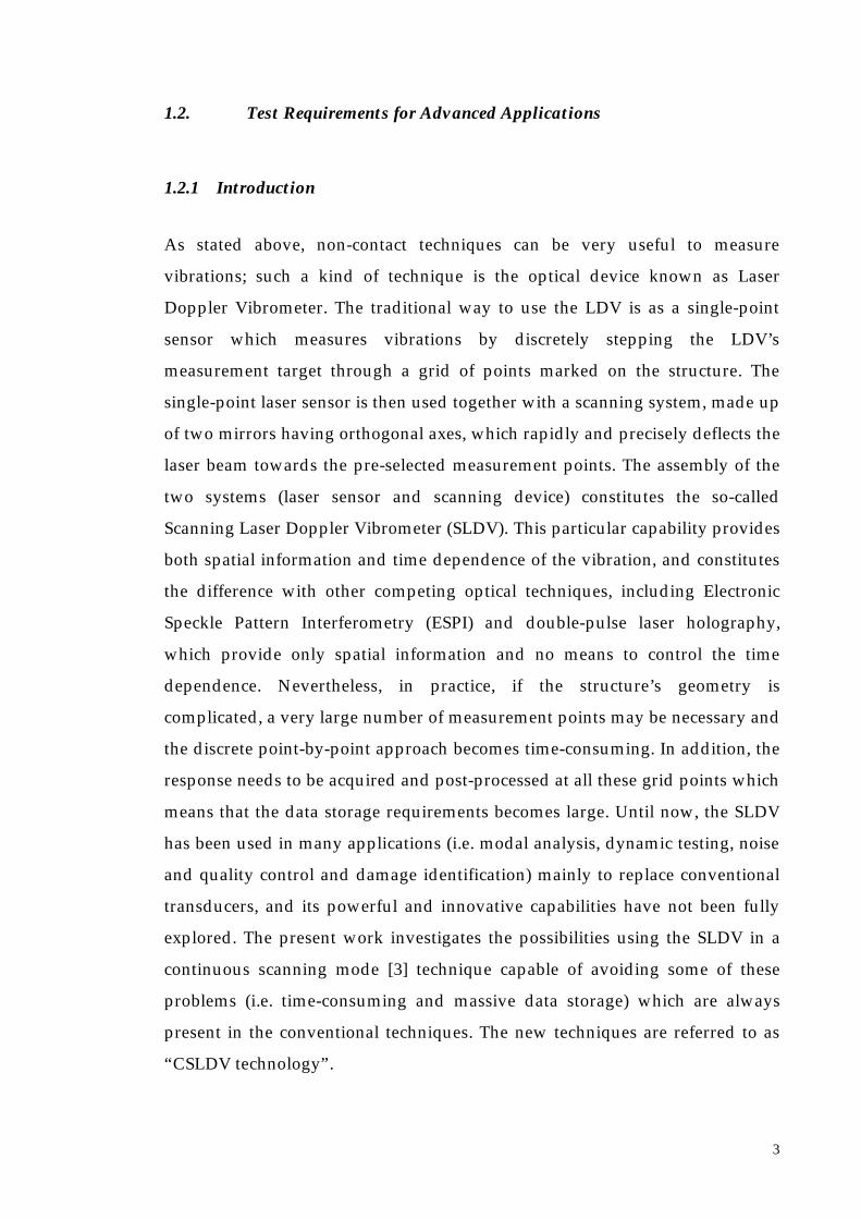
1.2.1 Introduction

As stated above, non-contact techniques can be very useful to measure

vibrations; such a kind of technique is the optical device known as Laser

Doppler Vibrometer. The traditional way to use the LDV is as a single-point

sensor which measures vibrations by discretely stepping the LDV’s

measurement target through a grid of points marked on the structure. The

single-point laser sensor is then used together with a scanning system, made up

of two mirrors having orthogonal axes, which rapidly and precisely deflects the

laser beam towards the pre-selected measurement points. The assembly of the

two systems (laser sensor and scanning device) constitutes the so-called

Scanning Laser Doppler Vibrometer (SLDV). This particular capability provides

both spatial information and time dependence of the vibration, and constitutes

the difference with other competing optical techniques, including Electronic

Speckle Pattern Interferometry (ESPI) and double-pulse laser holography,

which provide only spatial information and no means to control the time

dependence. Nevertheless, in practice, if the structure’s geometry is

complicated, a very large number of measurement points may be necessary and

the discrete point-by-point approach becomes time-consuming. In addition, the

response needs to be acquired and post-processed at all these grid points which

means that the data storage requirements becomes large. Until now, the SLDV

has been used in many applications (i.e. modal analysis, dynamic testing, noise

and quality control and damage identification) mainly to replace conventional

transducers, and its powerful and innovative capabilities have not been fully

explored. The present work investigates the possibilities using the SLDV in a

continuous scanning mode [3] technique capable of avoiding some of these

problems (i.e. time-consuming and massive data storage) which are always

present in the conventional techniques. The new techniques are referred to as

“CSLDV technology”.

4

1.2.2 Need for Non –Contact Measurements Devices

In conventional vibration tests, accelerometers are commonly used to acquire

acceleration time histories at selected locations. These devices are a source of

error when lightweight structures are examined because the local mass loading

of the sensor may distort the results or when fluid flows are studied since the

introduced transducer disturbs the flow itself. In the first case, a non-contact

sensor is essential and in the second a non-invasive transducer is needed. The

Laser Doppler Vibrometer (LDV) introduced by Yeh and Cummins (1964), [4],

is an optical velocity-measuring device which satisfies both the characteristics

demanded above. This device is based on the measurement of the Doppler shift

of the frequency of laser light scattered by a moving object. One of the first

applications of the LDV in vibration measurement fields was in the context of

extremely lightweight objects such as fibre velocities measurement in spinning

and drawing processes in man-made fibre production, [5].

1.2.3 Need for Spatially–Dense Measurements

Many applications of structural vibration tests require spatially dense

measurements, where a surface is surveyed with high spatial resolution and a

lot of points over the area need to be investigated. The velocity distribution

measured over the surface at a given frequency and referred to a reference

signal is called “Operating Deflection Shape” (ODS) or simply, less precisely,

“Mode Shape”. In this case the mode shape is the vibration pattern on the

surface and it is different from the normal modes or eigenvectors which

represent the free-vibration solution, together with the eigenvalues (natural

frequencies and damping factors). A two-dimensional ODS can be measured

over a grid of measurement points using several accelerometers or a SLDV (i.e.

the laser beam moves discretely point by point). The latter technique permits a

higher resolution because the laser spot dimension is smaller than an

accelerometer, but the measurement process is still time-consuming.

Alternatively, by using a CSLDV, scans along a line or across an area can be

performed enabling mode shapes to be defined along the line or over the area

5

with only one measurement, [3]. In this way, the LDV can simulate a multitude

of transducers located at the area where the scanning is acted, see Figure 1.1.

Note that when the laser is scanning continuously the red points become closer

and closer.

Figure 1. 1 Virtual transducers location along the laser beam scan line.

The result of the measurement process is a modulated velocity time history

with the spatial variation in vibration amplitude being the modulation signal.

The physical meaning of the continuous scan is evident if the line scan is seen as

a series of consecutive points where the laser beam is moving discretely. When

the number of points increases towards infinity the scan becomes continuous.

The first point in the scanning line is the first location and the laser returns to

this point every cycle, the period of which is the inverse of the scanning rate. In

the first cycle the laser measures the first sample of the first, second, third …

points along the scanning line; on the second cycle the second sample of the

same points is acquired and so on. Without scanning continuously, the velocity

sensor is just waiting between samples, on the other hand, with scanning

continuously, it scans a number of measurement locations during this waiting

period. The response for a number of locations requires the same time to obtain

a single response on the discrete scanning technique. Moreover, when a set of

transducers are employed and they are positioned at discrete points along the

scan line, as the red dots show in Figure 1.1, even if the accuracy of the

measurement at each point is 100 %, there will be always an inaccuracy where

the measurement is not performed (between the transducers). On the contrary,

by scanning continuously, the ODS along the line can be recovered from the

x

yODS along

the line scan

VIRTUALTRANSDUCER

6

time signal measured, after some signal processing. The spatial definition of the

measurement points is, ideally, like going to infinity. In reality, the resolution

will be determined by the number of samples used in the acquisition of the time

history which could be very large with current commercially-available data

acquisition boards (above 500 KSamples per second).

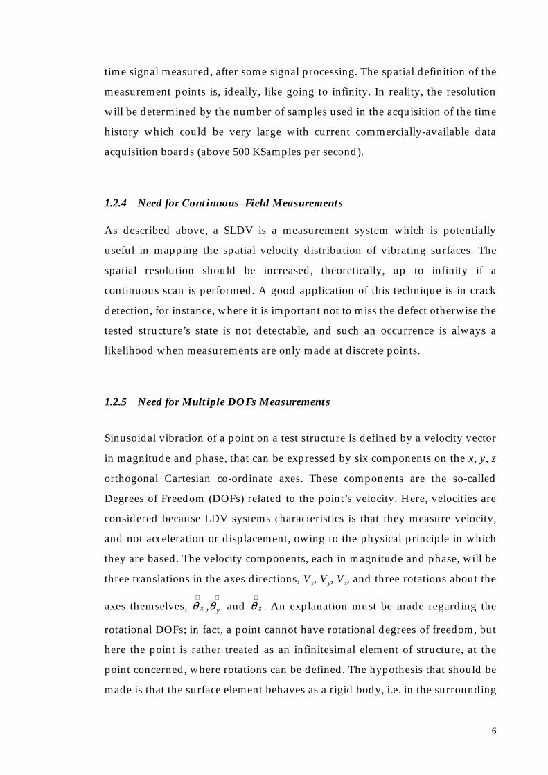
1.2.4 Need for Continuous–Field Measurements

As described above, a SLDV is a measurement system which is potentially

useful in mapping the spatial velocity distribution of vibrating surfaces. The

spatial resolution should be increased, theoretically, up to infinity if a

continuous scan is performed. A good application of this technique is in crack

detection, for instance, where it is important not to miss the defect otherwise the

tested structure’s state is not detectable, and such an occurrence is always a

likelihood when measurements are only made at discrete points.

1.2.5 Need for Multiple DOFs Measurements

Sinusoidal vibration of a point on a test structure is defined by a velocity vector

in magnitude and phase, that can be expressed by six components on the x, y, z

orthogonal Cartesian co-ordinate axes. These components are the so-called

Degrees of Freedom (DOFs) related to the point’s velocity. Here, velocities are

considered because LDV systems characteristics is that they measure velocity,

and not acceleration or displacement, owing to the physical principle in which

they are based. The velocity components, each in magnitude and phase, will be

three translations in the axes directions, Vx, Vy, Vz, and three rotations about the

axes themselves, ⋅⋅

yx θθ , and z

⋅θ . An explanation must be made regarding the

rotational DOFs; in fact, a point cannot have rotational degrees of freedom, but

here the point is rather treated as an infinitesimal element of structure, at the

point concerned, where rotations can be defined. The hypothesis that should be

made is that the surface element behaves as a rigid body, i.e. in the surrounding

7

of the specific point the surface is planar and is not subjected to any

deformation. Information related to the ‘rotational degrees of freedom’ (or

RDOF) is often required, for example when acquiring data for sub-structure

coupling calculations.

If an LDV beam scans continuously along a short line or around a circle over a

small element (with linear dimension sufficiently small, i.e. the surface is

treated as rigid body) of a harmonically-vibrating surface, its output will be

modulated in such a way that can be used to analyse structural vibration in

more than one DOF. Linear scanning enables two vibration components to be

measured: the translation velocity in the direction perpendicular to the surface

and the angular velocity about the direction lying on the surface plane and

perpendicular to the line scan. Using circular scanning, two angular vibration

DOFs about two mutual orthogonal axes lying in the plane of the test surface

can be derived directly from the frequency spectrum of the laser output,

together with the translational DOF in the direction perpendicular to the

surface itself. A further continuous scanning technique is one where the laser

beam scans on a circle over a short-focus lens so that the focal point is scanned

in a circular cone. This technique will be named conical scan and it will be

applied to recover three translation vibration DOFs at the point where the cone

vertex is hitting the test surface, i.e. the measurement point.

1.3. Objectives of Research Project

The specific objectives of this research work derive from the intention of

investigating the CSLDV technique which can be the answer to the demands of

the advanced applications highlighted in the previous section. These objectives

can be summarised as:

1. development of the CLSDV techniques for MDOF vibration response and

ODS measurements;

2. simulation of the CSLDV techniques;

3. experimental validation of the CSDLV techniques;

4. application of the CSLDV techniques in industrial cases

8

1.4. Literature Review

The aim of this thesis is to give a comprehensive description in both

mathematical and experimental points of view of continuous scanning laser

Doppler vibrometry. Moreover, the work done within this research includes the

development of the software to perform the control and the acquisition

processes during a CSLDV test.

Previous work found in the literature are mostly done by A. B. Stanbridge [49]

who first, used a microphone scanning on a circular pattern near a disc-like

structure in 1979, at Rolls-Royce Small Engine Division.

Early works concerning continuous scanning laser Doppler vibrometer were

realised by Sriram and al. in 1990-92 when the laser beam was made to scan by

means of an oscillating external mirror, [10], [11] and [12].

The use of an LDV was applied to the continuous circular scan performed on

rotating disc in 1994 by Bucher et al. in [6] and in 1995 by Stanbridge and

Ewins, [7]. MDOF vibration response measurements were first attempted in

1996 by Stanbridge and Ewins by using small linear and circular scans, [8], and

a conical scan [9]. The first stage of the research on ODS measurement was

carried out in 1996 [3].

Further investigations of the CSLDV technology were undertaken within the

BRITE/EURAM project VALSE, [13], by Stanbridge, Martarelli and Ewins and

the research developed were published in several papers ([14]- [19]) and

technical reports ([20]- [23]).

1.5. Structure of Thesis

The work reported in this thesis has been divided into four main sections:

a) an introduction to laser Doppler vibrometry, which is dealt in Chapter 2,

and, in particular, a critical assessment of the state-of-the-art of the scanning

laser Doppler technique as applied in some commercially-available LDV

such as the Polytec LDVs. The description of this is addressed in Chapter 3;

9

b) the analysis of the continuous scanning laser Doppler technology used for

MDOF vibration response measurement (described in Chapter 4) and for

ODS measurement (to which Chapter 5 is entirely devoted). This section

constitutes the heart of the thesis where each CSLDV technique is critically

analysed and validated being applied to simulated and experimental data;

c) the numerical simulation of a complete CSLDV test which is helpful to

rehearse the experiment before going to the laboratory. This operation, so-

called “virtual testing”, is described in Chapter 6;

d) the application of the CSLDV techniques to practical cases used to prove the

functionality of the techniques in operating conditions. Chapter 7 describes

the experimental cases studied and the different CSLDV techniques used.

A summary of each chapter is given here.

Chapter 2 describes, first, the principles on which the laser Doppler vibrometry

is based such as the Doppler effect and the laser light behaviour. Considerable

emphasis is given to the analysis of speckle noise, which is an unavoidable

phenomenon occurring when a coherent light beam is scattered back from an

optically rough surface. The effects produced on measured data by the speckle

noise are studied and, in particular, the frequency broadening of the LDV

output spectrum is addressed. This effect is markedly visible in the

experimental data, and so a through understanding of the phenomenon is

important. Secondly, the principal LDV configurations are presented: the

Michelson’s and the Mach-Zender interferometer. Finally, the working

principles of two LDV systems available on the market, the Polytec and the

Ometron LDVs, are outlined and a comparison between the two is deduced by

applying them to an identical experimental case.

Chapter 3 presents the scanning technology applied to the LDV systems and,

specifically, the technology used by the commercial system produced by

Polytec. This chapter aims to describe the state-of-the-art of the scanning LDV

where the term “scan” means that the laser beam moves point-by-point in a

10

grid of discrete points recording at each time the velocity of the point. The laser

beam acts as a transducer which measures at different positions over the tested

structure with the advantages of its non-contact nature and the automation of

the acquisition on the whole set of points. Several additional features available

in the Polytec system for improving the quality of measurement data are

addressed as well.

Chapter 4 is completely devoted to the mathematical investigation, simulation

and experimental validation of CSLDV techniques, when applied to MDOF

vibration response measurement. Since the laser beam is scanned continuously

along short pattern (lines or circles) in the proximity of the measurement target

point on the test structure in order to derive from the LDV output the

translational and angular vibration at that point, these CSLDV techniques are

classified as short scanning techniques. They include:

(i) short linear scan for measuring one translational and one angular

component of the velocity at a point;

(ii) small circular scan for measuring two translational and one angular

component of the velocity at a point;

(iii) conical scan for measuring the three translational components of the

velocity at a point;

(iv) conical-circular scan for measuring the three translational and two

angular components of the velocity at a point.

The calibration process of the technique is described, here, in order to provide a

definition of the performance of CSLDV technology and an outline of the

accuracy of the measured data. The analysis of speckle noise in relation to

experimental parameter settings as the scan speed is included, this noise being

the most important parameter affecting the accuracy of the measurement.

Chapter 5 is focused on the description of the CSLDV techniques used for ODS

measurement. In this case the laser beam is scanned continuously over a long

line or a large circle or even on a 2-dimensional pattern across a whole area.

While the laser beam travels along the test surface, the velocity measurement is

11

acquired continuously and from these data the ODS of this surface can be

derived. The final result, achieved in few seconds, is an ODS plotted with any

desired resolution over the measured surface. Different techniques (linear scan,

circular scan and area scan) are illustrated.

A large part of the chapter is devoted to the modal analysis applied to

“frequency response functions” (i.e. FRFs) data measured by the CSLDV

technique, with step-sine tests. The aim of this section is to prove the

advantages of using such kinds of FRF, specifically, the small amount of data

needed to be recorded and the time saving in both the acquisition and the

modal analysis processes.

Chapter 6 presents a numerical simulation of a complete CSLDV test. The

mathematical model of an ideal test is, first, derived and, subsequently, models

of the sources of noise are included with emphasis given to speckle noise.

Comparison between experimental simulated data and real measured data is

carried out in order to establish the level of agreement between numerical and

measured results.

Chapter 7 consists of a collection of experimental applications. Several

experimental structures were studied and different CSLDV techniques were

applied on them:

(i) short-line and small-circular scanning techniques for MDOF vibration

response measurement;

(ii) uniform-rate straight-line scan for ODS direct measurement via

demodulation of the LDV time history;

(iii) sinusoidal straight-line scan for polynomial ODS recovery;

(iv) parallel sinusoidal straight-line scan for 2-dimensional polynomial ODS

recovering;

(v) uniform-rate area scan for 2-dimensional ODS direct measurement via

demodulation;

(vi) sinusoidal area scan for 2-dimensional polynomial ODS determination.

Chapter 2 LDV Theory

2.1. Introduction

Laser Doppler Vibrometry is a well-established technique, based on the

Doppler effect, as its name suggests. This phenomenon appears in any form of

wave propagation where relative motion of source and receiver causes

frequency shifts related to the relative velocity; by measuring the frequency

change the velocity may be easily derived. In the LDV technique there is no

relative movement of source and receiver: the moving object is a solid surface

placed between them where the light is scattered. Rearranging the Doppler

formulae in the case of scattering the velocity of this surface, which constitutes

the tested object, can be recovered.

Only the invention of lasers made the exploitation of the Doppler technique to

measure velocities possible since the existing electromagnetic radiations (infra-

red, visible regions and beyond) could not be generated in a controlled way: by

using thermal sources, referring on the thermodynamics principles, there is

always a limit to the concentration of energy that imply random amplitude and

phase fluctuations of the emitted radiation. On the other hand, lasers are

13

suitable to produce single frequency and constant amplitude oscillations in the

optical region with an increased energy density and, more importantly, with a

long coherence length.

Velocity measurement based on the Doppler effect cannot be applied directly,

being velocities commonly encountered very small with respect to the light

velocity and then Doppler shifts produced are small. In fact, the Doppler

frequency resulting from a velocity v of a solid surface can be derived from the

following linear relationship

( )λ

ϑcos2vfD = (2. 1)

v cos (ϑ) being the velocity component along the direction of illumination of the

laser beam when it is directed at the tested surface, see Figure 2.1, where a

schematic configuration of a LDV (Michelson arrangement) is shown. In most

cases the light reflected by the moving target is collected by a detector placed on

the same part of the source with respect to the target. Such receptive modality is

defined as “backscattering”.

Figure 2. 1 Basic LDV arrangement.

Assuming the solid surface of the moving target to be perpendicular to the

optical axis of the laser source (cos (ϑ) = 0° ) and its velocity to be 1 m/s, λ being

the wavelength of the light (632.8 nm for a He-Ne laser source) the

correspondent Doppler shift will have a value of 3.17 106 Hz which is extremely

small in comparison to the He-Ne laser frequency 4.74 1014 Hz. Such a small

LASERSOURCE

BEAMSPLITTER

Referencebeam

Measuringbeam

PHOTODETECTORSPECTRUMANALYSER

MOVINGTARGET

v

ϑ

v cos(ϑ )

14

resolution can not be measured electronically; the highest resolution optical

spectrometer is neither suitable to detect such a small change in frequency.

Moreover, direct optical spectroscopy is an impractical technique, which is

exceptionally relegated to measure high velocities (i.e. supersonic). Only by

mixing the scattered light with a reference beam derived from the same

coherent source on the surface of a light detector producing an heterodyne or

beat of two frequencies in the output intensity, it is possible to recover from this

output the Doppler shift. In fact, the frequency of the signal coming from the

photodetector after the beating process is the difference between the two beam

frequencies and it is just the Doppler frequency. The photodetector is an opto-

electronic device which converts into an electrical signal proportional to the

variation of the optical signal intensity and therefore to the velocity of moving

scattering object. Using a conventional spectrum analyser, it is possible to

determine the beat frequency, bearing in mind that high frequency ranges may

be needed.

It is important to emphasize at this point that the optical beating technique can

be regarded as an interferometry principle and this is the reason why Laser

Doppler systems are usually called interferometers. Although this analogy

should be made only when optical surfaces are prepared in such a way to be

specularly reflective or, more likely, when tested objects move slowly, in the

thesis the term “interferometer” will generally be employed.

In this chapter, fundamental physical principles related with LDV methods are

addressed as the Doppler phenomenon (which constitutes the basis of the

measurement operation) and laser speckle, which is a property of coherent

monochromatic light scattered back from a rough surface on the scale of the

optical wavelength. The most common configurations of the LDV are then

described, i.e. Michelson and Mach-Zehnder Interferometer), together with

some devices, which are capable of discriminating the direction of the velocity

which is a peculiar problem in all beating techniques. Acousto-optic devices,

such as the Bragg cell, are the most commonly used for this purpose and they

15

are hereafter afforded special attention. In conclusion, the two LDVs, which are

commercially available are highlighted: Polytec and Ometron systems.

2.2. Doppler Effect

2.2.1 Introduction

The so-called “Doppler shift” is a phenomenon which arises when there is a

relative motion of the source and the receiver of a wave propagating from one

of them: the effect is a change in apparent frequency of the wave seen by the

receiver. Such situation may be achieved having a stationary source and a

moving observer or a moving source and a static observer but it can be

extended to the case where the moving part is an intermediate object through

which wave motion is transmitted from the source to the receiver. The latter is

the common phenomenon realised in Laser Doppler devices, [4].

2.2.2 Stationary Source-Moving Observer

A stationary source S of light waves of wavelength λ and velocity c and a

moving observer O, endued with velocity u are considered, see Figure 2.2. The

wave-front of the light in the neighborhood of O is supposed to be plane, the

distance SO being large. With the observer O travelling towards the source, it

will intercept the wave fronts at a higher frequency, the frequency shift being

∆f.

( ) ( )c

uf

uf

ϑλ

ϑ coscos ==∆ (2. 2)

where ϑ is the angle between the direction of the observer motion and the

direction of the wave propagation and f is the frequency of the emitted wave.

16

Figure 2. 2 Doppler effect (Stationary Source-Moving Observer).

2.2.3 Moving Source-Stationary Observer

The opposite situation deals with a moving source which transmits lightwaves

of frequency f and velocity c, to a stationary observer; the relative motion of

transmitter and receiver is the same in both cases but the formula describing the

frequency shift appears more complicated:

( )

( )ϑ

ϑ

cos1

cos

c

uc

u

f

f

−=∆

(2. 3)

This expression can be made to agree with the previous one, with the

assumption of u being small velocity compared with c, by expanding it in

Taylor power series in u/c and neglecting the higher order addends:

( ) ( ) ( ) ...coscoscos 33

22

+

+

+=∆ ϑϑϑ

c

u

c

u

c

u

f

f(2. 4)

2.2.4 Scattering Condition

The third Doppler situation occurs when a lightwave is emitted from a

stationary source and received by a moving object, which then retransmits to a

stationary observer. This circumstance can be visualised as split into two stages:

in the first step, there are a stationary source and a moving observer (which is

OS

uϑ

17

the inert object) and in the second step, the inert object behaves as moving

source, by reflecting to the receiver the incident wave. This is a combination of

the two previous configurations and can be described as a “double Doppler

shift” and is illustrated in Figure 2.3.

Figure 2. 3 Doppler effect (Scattering Condition).

The global situation can be decomposed into two configurations, i.e. (i) and (ii):

(i) A stationary source S emits lightwaves at frequency f and velocity c,

which are scattered by an observer T moving at velocity u. The wave

frequency received by this latter would be shifted following Equation

(2.1) and it will be f+∆f:

( ) ( )

+=+=∆+= 11 cos1cos’ ϑϑ

c

uf

c

ufffff (2. 5)

ϑ1 being the angle between the direction of motion and the direction of

waves coming from S.

(ii) Now the target T re-emits the light at frequency f ’ and it behaves as

moving source which is reflecting the waves towards the steady observer

O with a frequency shift given by Equation (2.2). The final frequency will

be:

O

TS

u

ϑ1

ϑ2

18

( )

( )

( )

( ) ( )

−=

−+=

−+=∆+=

22

2

2

2

cos1

1’

cos1

cos1’

cos1

cos’’’’’’

ϑϑ

ϑ

ϑ

ϑ

c

uf

c

uc

u

f

c

uc

u

fffff (2. 6)

Introducing Equation (2.3) into (2.6) the final Doppler frequency will

become:

( )

( )

−

+=

2

1

cos1

cos1’’

ϑ

ϑ

c

uc

u

ff (2. 7)

and, for small velocities compared with c, expansion in a Taylor power

series can be applied, so that, neglecting higher order terms:

( ) ( ) ( ) ( )

( )

( ) ( )( )c

u

c

u

c

u

c

u

c

u

c

u

c

ud

f

fd

c

u

c

ud

f

fd

f

f

c

u

c

u

c

u

21

0

2

2

2112

2

0

2

2

0

coscos1

cos1

coscos1coscos11

...

’’’’

1’’

ϑϑ

ϑ

ϑϑϑϑ

++=

=

−

++

−

+=

=+

+

+=

=

==

(2. 8)

The final expression for the scattering Doppler shift results as:

( ) ( )( )2

cos2

cos2

coscos’’ 212121

ϑϑϑϑλ

ϑϑ −+=+=−=∆ u

c

uffff (2. 9)

In the special case when the source and the receiver are positioned close to each

other, as in the LDV configurations available, ϑ1 and ϑ2 coincide and the

conventional formula returns:

19

ϑλ

cos2u

f =∆ (2. 10)

Velocity measurements made by means of an LDV exploit the above-illustrated

physical principle where the wave source is a laser and the receiver is a

photodetector which measures the target surface velocity related to the Doppler

shift.

2.3. Laser Light

Light is an electromagnetic wave arising from interaction of electric and

magnetic fields, although in optics magnetic component fluctuation is

negligible. The propagation of the light is, then, expressed by the solution of

Maxwell’s equations, which is, for a plane monochromatic wave of frequency f

and wavelength λ propagating in z direction, neglecting polarization effects:

( )

++= ϕπ

λπ

tfzEtzE 22

cos, 0 (2. 11)

where ϕ is a phase constant, E0 the amplitude of the electric field and 2π/λ is the

so-defined wave-number k. Such a wave is an idealisation, which is

satisfactorily approached by laser sources.

As the wave advances, the sinusoidal pattern moves along z at velocity c that

depends on the propagation medium. If it is the vacuum c will assume the

value of 2.997 108 m/s. The wave oscillation is described in Figure 2.4.

20

Figure 2. 4 Electric field fluctuation along its direction of propagation.

In lightwaves theory, in order to simplify the analytical dealing with the electric

field, a complex notation is introduced:

( ) ( )[ ] ϕπ ++= tfkziEtzE 2expRe, 0 (2. 12)

The physical quantity electric field is represented by the real part of the

complex expression E0 exp[i ( kz + 2π f t + ϕ )]. Calling A the complex amplitude

of the lightwave:

( ) ( )[ ]ϕ+= kziEzA exp0 (2. 13)

the analytical signal describing the electric field is

[ ]tfiA π2exp=Ε (2. 14)

whose real component represent the physical quantity.

Light is then regarded as the oscillation of the electric field described above. In

LDV techniques the light contains the sought velocity information; having this

oscillation too high frequency to be oserved by available detectors, it is usual to

0 0.2 0.4 0.6 0.8 1

-1

-0.8

-0.6

-0.4

-0.2

0

0.2

0.4

0.6

0.8

1E0

- E0

z

E

t t + ∆t

21

record its intensity that result to be proportional, by the light velocity, to the

square of its complex amplitude:

*AAI ∝ (2. 15)

In order to perform velocity measurements using the beating of two lightwaves

these latter must have long coherence length, that is the length of the optical

path in which a constant phase relation exists between the two lightwaves. In

fact interference phenomena can only be observed with coherent waveforms.

Another requirement for the light source is to be single frequency. The spectral

purity of the light source influences indeed the broadening of the measured

Doppler spectrum, together with other factors such as optical imperfections,

and velocity fluctuations. The broadening effect consists on a spread of the

Doppler signal spectrum around the Doppler frequency; if this widening of the

frequency peak becomes too large the spectrum can not be clearly interpreted to

give the velocity information.

Laser sources meet these requirements with their spatial and chromatic

coherence. They operate by the principle of Light Amplification by Stimulated

Emission of Radiation. The amplifying medium, commonly an atomic or

molecular gas at low pressure, is contained inside a long discharge tube. When

the electric discharge is operated the gas excitation becomes a light amplifier. A

cascade process starts: spontaneous emission causes stimulated emission which

is amplified as it reflects back and forth many times through the amplifying

medium by two high-reflectivity mirrors placed at the ends of the discharge

tube. The space contained between the two mirrors is called optical resonator

cavity. The resonator action of the optical cavity swamps out the random nature

of the spontaneous emission and the light passing through the end-mirrors

owns high spatial coherence. In practice lasers own a multi-mode frequency

output although there is a dominant transverse mode, which allows to neglect

all the others. This uniphase mode, so-called TEM00 , yields a Gaussian light

intensity distribution circularly symmetrical for the output beam. However

22

lasers operating in multi-mode are employed especially for large power

requirements.

A monochromatic electromagnetic radiation with Gaussian profile of width w

and radius of curvature σ at a point r in the space (r is the vector position), see

Figure 2.5, can be expressed as:

( )

−

= 2

22

0

rexp

rexpr

w2

ikEE (2. 16)

The width w at the point r away from the laser beam waist of the distance z

could be expressed as a function of w0 or beam width at its waist.

2

2

0 1a

zww += (2. 17)

where

λπ 2

0wa = (2. 18)

and λ is the laser wavelength.

Figure 2. 5 Gaussian light beam profile.

From the laser source w0

z

w Gaussiandistribution

23

2.4. Laser Speckle

When coherent light is scattered from an optically rough surface a laser speckle

pattern is formed in space in front of the target, [24]. Optically rough surface is

a requirement, which is accomplished when the micro-size of the surface

roughness is equal or bigger than the wavelength of the illuminating source,

according to the “Rayleigh criterion”, which says that a surface tend to be

effectively smooth only if the ratio between its irregularities height and the

wavelength of the incident beam tends to zero. Thus all but the quite highly

polished optical surfaces are candidate to realise the condition for speckle

pattern formation, hinting at the conclusion that speckle is unavoidable. The

usual appearance of speckle pattern is granular since it is produced by the

constructive and destructive interference of the coherent light scattered by the

optically rough surface within the illuminated area of the structure. The

phenomenon occurs because each microscopic element of the scattering surface

within the laser spot acts like a point source of coherent light. At a point in

space, individual scattered wavelets from these sources interfere constructively

or destructively to produce the bright or dark speckle observed on the screen.

The speckle pattern is a continuous random distribution of light amplitude and

phase although in practice the quantity observed is the corresponding intensity

distribution. The speckle effects are characteristic of monochromatic light and

are particularly noticeable with laser sources. When the light contains a broad

band of frequencies the speckle patterns for the different frequencies will differ

and the effect averages out.

In Speckle Interferometry laser speckles are the information carriers: when the

surface moves, the speckle created by the surface also moves, and the resulting

changes in phase relationships within individual speckles cause changes in the

speckle irradiances. In speckle interferometries, the irradiance change in each

speckle is used to measure the displacement (deformation) of the object at that

speckle. Thus the essence of the measurement is the monitoring of brightness

24

changes in each and every speckle, corresponding roughly to each pixel, in a

video image of the object.

On the other hand, Laser Doppler Vibrometry investigate the resultant Doppler

beat signal coming from the diffusely reflecting object. The signal is then

deteriorated by the so-called “speckle noise”, which appears as a dropouts of

the signal when the light intensity is low (“dark” speckle). The speckle pattern

dynamics, reducing accuracy of measurement, limits the performance of the

laser system, indeed.

The most important property of the speckle that influences LDV measurements

range is the speckle size1 defined as a statistical average of the distance between

adjacent regions of maximum and minimum brightness. This property can be

statistically estimated from the space correlation function of the light scattered

from a rough surface. Statistical properties of dynamic speckles produced by a

diffuse object, which undergoes constant velocity motion within its own plane,

have been intensively studied by E. Jackeman, J. G. McWhirter, [25], T. Asakura

and N. Takai, [26] and J. H. Churnside, [27]. It is important to remark that if the

object illuminated by the coherent light is motionless the scattered light forms a

“stationary speckle pattern” which becomes “dynamic” when the object starts

to move with an in-plane velocity. In fact the speckle pattern will move in the

same direction of the target motion.

As the diffuse reflecting object, where the light is scattered, a model of the deep

random phase screen is very often employed: recurring to light-scattering

theory, the deep random phase screen is defined as a thin scattering layer which

introduces randomly fluctuating path differences into an incident

electromagnetic wave. The random phase fluctuations are considered to be

Gaussian distributed. The diffuse object is supposed to move with a constant

velocity at the object plane. In this situation two different fundamental motions

of speckles are produced:

1 LDV measurements are also influenced by the speckle amplitude and, in particular, phase since mostcommercial instruments work with one speckle on the detector. If the speckle moves off the detector andis replaced by another, a dark speckle will produce a drop out. If a series of different bright speckles movewithin the detected area the phase distribution will change randomly [50].

25

1. for considerable displacement of the diffuse object the speckles move as

whole and their shape remains unchanged. This type of speckle motion is

called translation of speckles.

2. in other cases, as the diffuse object moves, the individual speckles deform,

disappear, and reappear without appreciable displacement of their

positions. This type of speckle motion is called boiling of speckles.

These motions are strictly related to the diffuse object movement but also to the

optical parameters (w, σ) and to the distance between the object and the

detector (R). In practise the speckle translation appears in near-field conditions

(observation position close to the object), while the boiling is predominant

when the detector is far apart from the moving target (far-field conditions).

Dynamic speckles are then investigated in the diffraction field with the Fresnel

diffraction approximation:

1. the distance between the observation plane, where the detector receiving the

scattered light from the object is placed, and the diffuse object is finite;

2. the distance between the observation plane and the diffuse object is greater

than the largest linear dimension of the lluminated region on the target; and

3. the propagating wave is assumed to be spherical.

A complex Gaussian beam, see Equation (2.16), will be employed for

illumination since such a Gaussian beam can be easily obtained with a TEM00

mode for the laser. The light scattering configuration is described in Figure 2.6.

Figure 2. 6 Light scattering and light collection process.

PhotodetectorLight collected

E(R)

w0

z

w

v

R

θ Rigid deeprandom-phasescreen

Incident Gaussian beam E0

LightscatterdE(r)

26

When the diffuse object moves with the in-plane velocity v the light emergingfrom it will be:

( ) ( ) ( )[ ] ( )

( )[ ] ( )tititw2

kiE

titiEtE

ωφ

ωφ

−−

−

=

=−−=

exprexpr

expr

exp

exprexprr,

2

22

0

0

v

v

(2. 19)

where φ(r) is the randomly varying position-dependent phase shift caused by

transmission through the moving screen and r being the position of the object

where the beam is scattered. The phase fluctuation φ produced by the diffuse

object is strictly related to its velocity v.

In accordance with the Huygens-Fresnel principle, [28], the field in the

observation point, defined by the vector position R (being R its amplitude), is:

( ) ( )( )∫∞

∞−

−+= rrRexpcos1r,

2

1R, 22

dR

itEtE

λπθ

λ (2. 20)

where the propagation in the mean between screen and detector is assumed in

the Fresnel approximation (i.e. the observing screen of the scattered wave is at a

finite distance from the scattering surface). The propagation function is then

expressed as:

( )

−= 2

rRexpRr,R

ih

λπ

(2. 21)

After some manipulations the field detected at R will become:

( ) ( ) ( ) ( )( ) rrRexpr

expr

exprexpexp2

cos1R, 22

2

2

20 d

R

i

2

ki

wtiti

EtE ∫

∞

∞−

−

−−−+=

λπφω

λθ

v

(2. 22)

27

Dependence on the angle θ, between the optical axis of the incident beam and

the detector direction, appears on the observed field expression.

The speckle intensity detected at the point R on the detector surface will

fluctuate randomly in space and in time being scattered by the diffuse object.

Under the hipotesys of incident Gaussian beam with zero mean the space-time

correlation of the speckle intensity detected can be formulated as:

( ) ( )τ+tEtE ;R;R 2*

1 (2. 23)

where ⟨⟩ stands for an ensamble average. The correlation is done between the

field in two points on the detector surface R1 and R2 and in two instants t and

t+τ.

Normalising the previous expression:

( ) ( ) ( )( ) ( )

( ) ( )( )tI

tEtE

tEtE

tEtEg

;0

;R;R

;0;0

;R;R;R,R

2*

12*

1

21

τττ

+=

+= (2. 24)

being

( ) ( )[ ] 2;0;0 tEtI = (2. 25)

and substituting Equation (2.22) in (2.24) the final formulation for the

correlation function can be derived:

( )

−−−

−= 2

1222

22

2

22

21 RRexpexp;R,R τλπττ v

R

w

w

vg (2. 26)

The in-plane velocity v of the screen appears in the previous expression thus it

is experienced by the detected light which constitue the signal output from the

detector.

28

The statistical properties generally analysed are the correlation time length τC

obtained by putting R1 and R2 equal zero in the space-time correlation function

(time-correlation function g(0,0;τ)) and the correlation length ∆x obtained by

setting τ equal zero in the same function, i.e. the space correlation function

g (R1 , R2 ;0) is derived.

The time correlation function will be

( )

−=

−−

−= 2

22

22

22

2

22

expexpexp;0,0cR

w

w

vg

τττ

λπττ v (2. 27)

from which the time correlation lenght τc can be derived. This parameter has

the phisycal meaning of the transit time of a single speckle across the detector

(i.e. time taken for a speckle grain to advance across the receiving area on the

detector by one speckle length).

The space correlation function will be

( )

−−= 2

1222

22

21 RRexp0;R,RR

wg

λπ

(2. 28)

where the quantity

w

RS

πλ= (2. 29)

is the correlation length which is strictly related to the speckle size formed in

the diffraction field. Within this correlation region the amplitude and phase of

the light may be assumed to be constant. In fact, intutitively, if the speckle is

larger (larger S) the two detectors placed in R1 and R2 will measure the same

speckle then the speckle intensity correlation is bigger. At points on the

29

observing screen closer than S there is a consistent phase relation between light

received from all scattering particles and thus the intensity of illumination is

substantially constant. For points far apart, phase correlation is lost and the

intensity is in general different. Thus “speckly” illumination is obtained.

For a Helium-Neon laser source of wavelength of 632.8 nm and beam width at

its waist of 0.08mm, if the laser source is placed at such a distance from the

object that the beam waist is away from it of the length of 300 mm, the laser

beam width on the object is 0.7556 mm (w). Placing the detector at 1 m from the

object it is easy to calculate the average speckle size which is 0.2667 mm.

To the speckle pattern is related the Laser noise which affects measurements in

fact, if the detector observes more than one speckle there is a large likelihood

that bright and dark areas are detected then the light intensity collected will

fluctuate between a minimum and a maximum. Because the device where the

analog velocity waveform is derived from the Doppler signal requires that the

Doppler signal exceeds an amplitude threshold, below this value the velocity

output will be dropped to zero or to a value less than reality and this effect is

called “drop-out”, see Figure 2.7.

Figure 2. 7 Velocity Drop out.

Signal dropouts affecting accuracy of the measurement appear if operation

distances are not optimal, the test surface is poor reflective or the measuring

beam is mis-focused, i.e. spot size on the object is large.

0 0.1 0.2 0.3 0.4 0.5 0.6 0.7 0.8-5

-4

-3

-2

-1

0

1

2

3

4

5

target velocityoscillation

drop out

velocityamplitude

time

30

The measurement laser spot should be as small as possible: the ideal situation is

achieved when the spot size is exactly the speckle size, allowing the detector to

receive just one bright speckle and the coherence to be maximum. Moreover if

the surface undergoes a sideways motion the illuminated area is changing

during the vibration and the speckle pattern varies at the same time. This

causes amplitude and phase detected become random. Increasing the

measuring spot size, the sensitivity to surface tilt increases as well, i.e.

maintaining the beam focused is an important task. An helpful expedient to

realise this task is to treat the structure’s surface in order to make it highly

diffusely retroreflective and then to increase the intensity of backscattered light.

The most commonly applied treatment is the surface coating with a developer

spray or retroreflective paper provided by LDV manufacturers. The result is

that the surface appear covered with fine matte particles which tend to

concentrate more of the scattered light into a restricted angle centered along the

laser beam line-of-sight. The Doppler signal level undergoes then an increase, in

average, which makes the signal itself more robust to changes in speckle

intensities resulting from the speckle motions generated during the motion of

the vibrating structure.

Because the speckle pattern, although random, does not change with time

unless the test surface is moved relative to the measuring beam, the occurrence

of dropouts is spatial and not temporal in nature, [29]. But there are cases where

the object is moving relatively to the beam (in-plain vibration or tilts) or vice

versa when the beam is scanning along the surface in which case the occurrence

of dropouts become periodic. If the surface is subjected to a sideways vibration

or if the laser beam is moving the speckle pattern will move with them. Then a

further kind of interference on the detected signal will occur: the so-called

speckle pattern motion, which is caused by the relative rotation or in-plane

translation of the illuminated area. The speckle motion will appear in the

output Doppler signal and it will affect the velocity measurement in such a way

as a pseudo-vibration, [50], is added to the true one, which is the target motion.

This motion mostly appears close to the structure nodes where the vibration is

31

almost zero but it involves rotation of the surface plane, then the sideways

motions are larger.

Speckle noise level found experimentally is always around 1% of the full scale

of measurement (-40 dB) as the application chapters show.

2.5. Frequency Broadening related to the Laser Speckle

The speckle intensity fluctuations produced in the diffraction field from an out-

of-plane vibrating object scattering a laser light (assumed to have a Gaussian

profile) is statistically investigated here. An effect strictly related to the speckle

can be identified which is the so-called “frequency broadening” of the detected

signal averaged power spectrum. This phenomenon is so-named since, under

certain conditions, the frequency spectrum of the LDV output contains not only

the component at the vibration frequency of the target, but also all its

harmonics. The analysis shows that the behaviour of the averaged spectrum is

determined by two physical parameters:

- the derivative value of the amplitude of the object vibration, and

- the beam width of light used for illumination.

It is especially noticed that the power spectral broadening width increases

linearly with the increase of these two factors.

Dynamic speckles were studied in detail by T. Asakura and N. Takay, [30],

since they were interested in applications to metrology. In fact, speckles

produced by a diffuse object contain information about its motion because the

space-time statistical properties of dynamic speckles depend on the velocity of

the moving object.

The intensity distribution of the speckle pattern formed at a certain receiving

plane (see Figure 2.8) in the diffraction field varies as a function of space and

time. This quantity is described in terms of:

32

- the intensity distribution of the illuminating beam arriving on the

moving object surface,

- the microscopic surface structure (roughness) of the illuminated object,

- the object vibration, and

- the propagation function of the linear optical system ( h(R,r) ), R and r

being the spatial position of the scattered laser light at the vibrating

object surface and the spatial position of the detected laser light on the

receiver surface, see Figure 2.8.

The illumination of the vibrating object will be modulated in two different

ways:

- one is a space-dependent phase modulation due to the surface roughness

of the object, and

- the second one is a space- and time-dependent phase modulation due to

the vibration of the object.

Figure 2. 8 Schematic of the laser optical path.

OUT-OF-PLANEVIBRATING OBJECT

RECEIVER PLANE

LINEAR OPTICALSYSTEMh(R,r)

R

r

33

The amplitude of speckle fluctuations detected at point r and time t may be

expressed as:

( ) ( ) ( )[ ] ( )[ ] ( )∫∞

∞−= dRrRhRtiRiRErte ,,expexp, 0 ψφ (2. 30)

where E0(R) denotes the amplitude distribution of laser light illuminating

the vibrating object,

φ(R) is a random phase variable obeying the microscopic random

structure of the surface roughness, i.e. it represents the space-

dependent phase modulation due to the surface roughness,

ψ(t , R) is the vibrating phase term linked to the object vibration,

i.e. it represents the space- and time-dependent phase modulation

due to the vibration of the moving object, and

h (R, r) is the propagation function of the point object from the

object plane to the receiving plane, characterising the light

propagation.

The vibrating phase term in cases of reflection can be given as:

( ) ( ) ( )00sin4

, θωλπψ += tRVRt (2. 31)

V(R) being the vibrating amplitude of the object,

ω0 the angular frequency of the vibration,

θ0 the initial phase of the vibrating object, and

λ the wavelength of light used for illumination.

Note that the spatial variation of ψ(t,R) depends on the vibration mode of the

object and is generally much less than the variation of φ(R) characterised by

the surface roughness of the object [30].

The intensity variation of the speckle will be given by:

34

( ) ( ) ( ) ( ) ( ) ( ) ( )[ ] ( ) ( )[ ] ( ) ( ) 212

*121

212*010

*

,,,,exp

exp,,,

dRdRrRhrRhRtRti

RRiRERErterterti

ψψ

φφ

−

−== ∫ ∫∞

∞− (2. 32)

Substituting Equation (2.31) into Equation (2.32), the term ψ(t,R) will appear as:

( ) ( )[ ] ( ) ( ) ( ) ( )[ ]

( ) ( ) ( )[ ] ( ) ( )[ ] ( )[ ]∑∞

−∞=

+

−=

−+=

=

+−+=−

nn tniRVRVJRVRVti

tRVtRViRtRti

00212100

00200121

exp4

sin4

exp

sinsin4

exp,,exp

θωλπθω

λπ

θωθωλπψψ

(2. 33)

where the exponential term is expanded with respect to time into the Bessel

series, which is:

( ) ( ) ( )∑∞

−∞=

=n

n inrJir θθ expsinexp (2. 34)

Jn(r) being the nth Bessel function of the first kind. If the vibration amplitude is

small within the illuminating light spot on the object the argument [V(R1)−

V(R2)] of the Bessel function can be approximated by

( ) ( ) ( )( ) ( ) ( ) ( )[ ]( ) ( ) ( )[ ] ...’’’

!3

1

’’2

1’

302

3010

202

201021021

+−−−+

+−−−+−=−

RRRRRV

RRRRRVRRRVRVRV(2. 35)

where V(R1) and V(R2) are expanded in a Taylor series around the central point

R0 of the beam. Assuming the vibration amplitude V(R) around R0 always

small, higher derivatives can be neglected, and Equation (2.32) becomes, then:

35

( ) ( )[ ] ( ) ( ) ( ) ( )[ ]

( ) ( ) ( ) 212*

1210

212*01000

,,4

expexp,

dRdRrRhrRhRRJ

RRiREREtinRti

n

n

−

−+= ∑ ∫ ∫∞

−∞=

∞

∞−

γλπ

φφθω(2. 36)

γ0 being the first derivative of the vibration amplitude of the object V’(R0) (i.e. its

vibration slope at the central position R0).

The power spectrum of the speckle intensity fluctuation detected at the point r

is obtained as:

( ) ( ) ( ) ( ) ( )[ ] ( ) ( )

( ) ( )[ ] ( ) ( ) ( )

( )[ ] ( ) ( ) ( )

( ) ( )[ ] ( ) ( ) ( ) 212*

121021

2*01000

212*

121021

2*01000

,,4

exp

expexp

,,4

exp

expexpexp,,

dRdRrRhrRhRRJRRi

EEdtintni

dRdRrRhrRhRRJRRi

REREdttintidttiRtirI

n

n

n

n

−−

−−

=

−−

+−=−=

∑ ∫ ∫∫

∑ ∫ ∫∫∫

∞

−∞=

∞

∞−

∞

∞−

∞

−∞=

∞

∞−

∞

∞−

∞

∞−

γλπφφ

ξξθωω

γλπφφ

θωωωω

(2. 37)

The time integral can be represented by the Dirac delta and Equation (2.37) can

be written as:

( ) ( ) ( ) ( ) ( )

( ) ( )[ ] ( ) ( ) ( ) 212*

121021

2*01000

,,4

exp

exp,

dRdRrRhrRhRRJRRi

REREinnrI

n

n

−−

−= ∑ ∫ ∫∞

−∞=

∞

∞−

γλπφφ

θωωδω(2. 38)

This is the power spectrum of the intensity of the speckle fluctuation at one

point at the detector surface; thus, in order to consider all the speckles an

averaged spectrum of the time-varying vibrating speckle intensity fluctuations

has to be performed:

36

( ) ( ) ( ) ( )[ ]

( ) ( ) ( ) ( )

( ) ( ) ( ) ( )[ ]

( ) ( )

( ) ( ) ( ) ( ) 432143*

2*

1

430’210

4321

4*0302

*010

’000

2

,,,,

44

exp

’exp’,

dRdRdRdRrRhrRhrRhrRh

RRJRRJ

RRRRi

RERERERE

nninnrI

nn

n n

−

−

+−−

−−−=

∫ ∫ ∫ ∫

∑ ∑∞

∞−

∞

−∞=

∞

−∞=

γλπγ

λπ

φφφφ

θωωδωωδω

(2. 39)

where the average is operated only in terms of the random phase variable

φ(R), which represents the roughness of the object surface. From the property of

the δ function the terms in the sum will be non-zero only if n = n’ and therefore

the averaged power spectrum will become:

( ) ( )

( ) ( ) ( ) ( )

( ) ( ) ( ) ( )[ ]

( )

( ) ( ) ( ) ( ) 432143*

2*

1

2102

4321

4*0302

*010

0

2

,,,,

4

exp

,


RRJ

RRRRi

RERERERE

nrI

n

n

−

+−−

−=

∫ ∫ ∫ ∫

∑∞

∞−

∞

−∞=

γλπ

φφφφ

ωωδω

(2. 40)

From the previous equation it can be seen that the averaged power spectrum

consists of discrete contributions of line spectra at angular frequencies as:

0ωω n= (2. 41)

which shows the property of periodically vibrating speckle intensity

fluctuations with the same periodicity as that of the vibrating object motion.

The magnitude of the averaged power spectrum at the spectral lines nω0 is:

37

( ) ( ) ( ) ( )

( ) ( ) ( ) ( )[ ]

( )

( ) ( ) ( ) ( ) 432143*

2*

1

2102

4321

4*0302

*010

,,,,

4

exp


RRJ

RRRRi

RERERERE

n

−

+−−

∫ ∫ ∫ ∫∞

∞−

γλπ

φφφφ(2. 42)

The amplitude of the Fourier components depends on the Bessel function of the

corresponding order and on the vibration slope γ0.

Equation (2.42) can be simplified by making some assumptions:

1. The phase variable φ(R) characterising the roughness of the vibrating object

surface follows a Gaussian behavior:

( ) ( )

−−=2

2

2exp

2

1

σµ

πσφ R

R (2. 43)

where ( ) ( )[ ] 2RR φφσ −= and ( )Rφµ = are the standard

deviation and the mean value of the distribution φ(ξ), respectively.

2. The random phase variable φ(R) is spatially stationary (i.e. σ and µ do not

depend on the spatial variable R ) and the surface is optically rough (i.e. the

roughness of the object surface is extremely fine compared to the size of the

illuminating beam). It can be then concluded that the phase variable φ(R )

has an extremely short correlation in space. Under these conditions, the

surface roughness is considered to have no correlation between two points,

which means that the normalised correlation may be set to

( ) ( )( )

≠=

=21

21

2

21

0

1

RRif

RRif

R

RR

φφφ

38

and the same can be written for the other positions (R3 and R4).

3. Under the hypothesis of the diffraction field, the propagation function

between the object and the receiving plane is given by:

( ) ( )

−

= 2exp, rR

R

irRh

λπ

(2. 44)

R being the distance between the object and the receiving plane and λ the

wavelength of the propagating light. The absolute value of this function

always equals unity whatever the receiving position is.

4. The illuminating light beam follows a Gaussian behaviour therefore the

intensity scattered out from the object will be:

( ) ( )

−−=

2

20

00 expw

RRII ξ 2. 45

where 0I and R0 are the central intensity and the central position of the

Gaussian beam, respectively, and w is the width of the beam at its

intersection with the object surface.

Equation (2.40), representing the averaged power spectrum of the speckle

fluctuation intensity, can be rewritten as [30]:

( ) ( ) ∫∑∞

∞−

∞

≠∞−=

−−= dRRJ

w

RInrI n

nn0

2

2

220

0,0

2 4exp, γ

λπωωδω (2. 46)

and its magnitude can be deduced as:

39

∫∑∞

∞−

∞

≠∞−=

− dRRJ

w

RI n

nn0

2

2

220

0,

4exp γ

λπ

(2. 47)

The parameters influencing the amplitude of the Fourier components are clearly

w and γ0 . No matter what values n assumes, if w (i.e. the size of the laser spot)

increases these Fourier amplitude components increase because the term

−

2

2

expw

R in Equation (2.47), see Figure 2.9.

Figure 2. 9 Gaussian function behavior varying the parameter w.

The parameter γ0 (the slope of the vibrating surface) is included within the

Bessel function that can be expressed as:

( )( )

sn

s

s

n Rsns

RJ2

00

0 2

4

!!

14+∞

=

+−=

∑ γ

λπγ

λπ

(2. 48)

-1 -0.5 0 0.5 10.3

0.4

0.5

0.6

0.7

0.8

0.9

1

−

2

2

expw

R

R

w

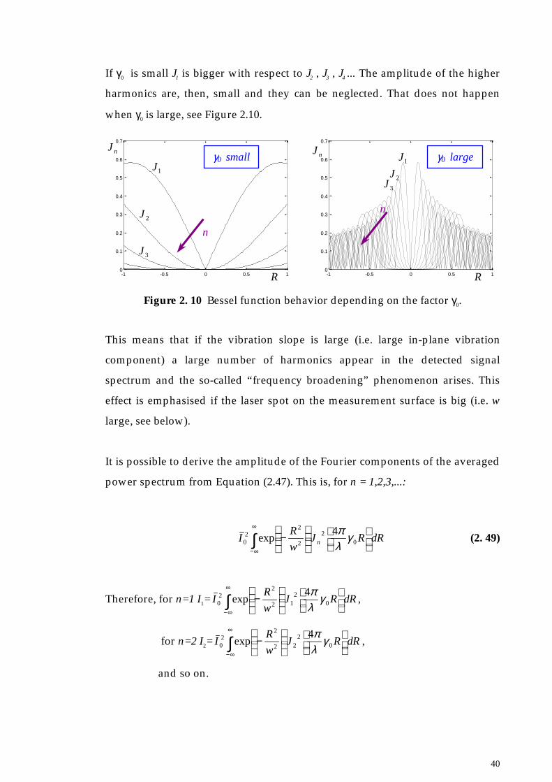
40

If γ0 is small J1 is bigger with respect to J2 , J3 , J4 ... The amplitude of the higher

harmonics are, then, small and they can be neglected. That does not happen

when γ0 is large, see Figure 2.10.

Figure 2. 10 Bessel function behavior depending on the factor γ0.

This means that if the vibration slope is large (i.e. large in-plane vibration

component) a large number of harmonics appear in the detected signal

spectrum and the so-called “frequency broadening” phenomenon arises. This

effect is emphasised if the laser spot on the measurement surface is big (i.e. w

large, see below).

It is possible to derive the amplitude of the Fourier components of the averaged

power spectrum from Equation (2.47). This is, for n = 1,2,3,...:

∫∞

∞−

− dRRJ

w

RI n 0

2

2

220

4exp γ

λπ

(2. 49)

Therefore, for n=1 I1= ∫∞

∞−

− dRRJ

w

RI 0

212

220

4exp γ

λπ

,

for n=2 I2= ∫∞

∞−

− dRRJ

w

RI 0

222

220

4exp γ

λπ

,

and so on.

-1 -0.5 0 0.5 10

0.1

0.2

0.3

0.4

0.5

0.6

0.7

R

nJ

1J

2J

3J

n

γ0 small

-1 -0.5 0 0.5 10

0.1

0.2

0.3

0.4

0.5

0.6

0.7

R

nJ1J

2J3J

n

γ0 large

41

Two cases are considered:

① w = 1 and γ0 = 1

② w = 10 and γ0 = 10

For the two cases the functions inside the integral are studied and they are:

−=

2

2

1 expw

Rf (2. 50)

and

= RJf n 0

22

4 γλπ

(2. 51)

Figure 2.11 shows the behaviour of f1 ( see the first plot) and f2 for n = 1, 2, 3 ( see

the second plot) in the first case (w = 1 and γ0 = 1). Figure 2.12 shows the

product f1 f2 and it is clear that this product quickly decreases as soon as n (the

order of the Fourier components) increases. In other words, the amplitude of

the averaged power spectrum is negligible for the higher harmonics.

Figure 2. 11 Gaussian and Bessel functions in the first case study.

-10 -5 0 5 100

0.1

0.2

0.3

0.4

0.5

0.6

0.7

0.8

0.9

1f1

R -10 -5 0 5 100

0.1

0.2

0.3

0.4

0.5

0.6

0.7

f2

R

n = 1

n = 2

n = 3

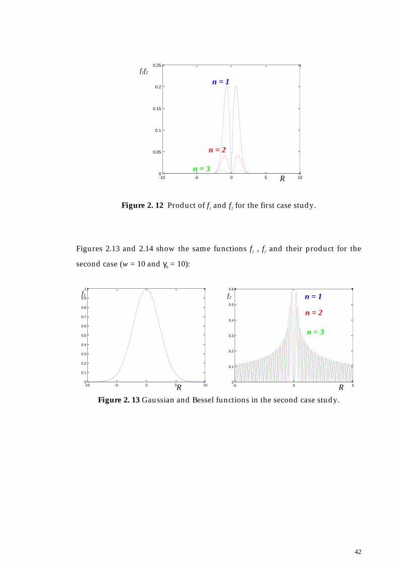
42

Figure 2. 12 Product of f1 and f2 for the first case study.

Figures 2.13 and 2.14 show the same functions f1 , f2 and their product for the

second case (w = 10 and γ0 = 10):

Figure 2. 13 Gaussian and Bessel functions in the second case study.

-10 -5 0 5 100

0.05

0.1

0.15

0.2

0.25

n = 1

n = 2

n = 3R

f1f2

-5 0 50

0.1

0.2

0.3

0.4

0.5

0.6

f2

R

n = 1

n = 2

n = 3

-10 -5 0 5 100

0.1

0.2

0.3

0.4

0.5

0.6

0.7

0.8

0.9

1

f1

R

43

Figure 2. 14 Product of f1 and f2 for the second case study.

It can be concluded that if w is small the spectral component at the fundamental

frequency (i.e. for n = 1) is dominant since the broadening of the Gaussian

function involved in the integral is small (see first plot in Figure 2.11). On the

other hand, for relatively large values of w the higher order spectral

components become more important as shown in Figure 2.14.

The amplitude of the averaged power spectrum is then shown for two more

realistic cases:

① w = 10 µm and γ0 = 0.0016 rad

② w = 100 µm and γ0 = 0.0028 rad

and Figure 2.15 shows the first 15 components of the averaged Fourier

spectrum. Note that in the second case the higher harmonics become significant.

The most important parameter which leads the analyisis is the laser beam

width, w. In fact, this latter governs the broadening of the Gaussian

function exp(-R2/w2). If the broadening of the Gaussian function is small it does

not matter how big the Bessel functions are (i.e. how large the vibration slope is)

-5 0 50

0.1

0.2

0.3

0.4

0.5

0.6

n = 1

n = 2

n = 3

R

f1 f2

44

because the product of the two functions (f1 f2) will emphasise only the centre of

the Bessel functions where the first order only has importance.

Figure 2. 15 Averaged power spectrum components for the two cases study.

Now, the laser beam illuminating the object plane is assumed to move along a

short straight line while the object vibrates out-of-plane at the frequency ω0. The

vibration experienced by the laser will be affected also by the rotation of the

object represented by the vibration slope γ.

The vibrating phase term as given by Equation (2.31) will be:

( ) ( ) ( ) ( ) ( ) ( )[ ]tRtltRVRt 00 sincossin4

, ωγωλπψ Ω+= (2. 52)

where V(R) is the vibration amplitude of the object,

γ(R) is the vibration slope,

ω0 is the angular frequency of the vibration,

Ω is the scan speed of the laser beam,

l is the scanned line length, and

λ is the wavelength of the light used for illumination.

θ0 is the initial phase datum, that is assumed zero.

Expanding out Equation (2.32) it will become:

0 1 2 3 4 5 6 7 8 9 10 11 12 13 14 150

0 1 2 3 4 5 6 7 8 9 10 11 12 13 14 150

n n

w = 10 µmγ0 = 0.0016 rad

w = 100 µmγ0 = 0.0028 rad

45

( ) ( ) ( ) ( ) ( )( ) ( )( )[ ]

−−++= ttR

ltRVRt ΩΩ 000 sinsin

2sin

4, ωωγω

λπψ (2. 53)

The exponential term including the vibration phase, ψ (R), examinated in

Equation (2.33) can be written as:

( ) ( )[ ] [ ( ) ( ) ( )[ ( )( )

( )( ) ] ( ) ( ) ( )[ ( )( ) ( )( ) ] ]

( ) ( ) ( )[ ] ( ) ( )[ ][ ( )( ) ( )( ) ]

( ) ( ) ( )[ ][ ]

( ) ( )[ ][ ( )( ) ( )( ) ][ ]

+−+−×

−=

=

+−+−+−=

=+−++−+

−++=−

ttRRl

i

RVRVti

ttRRl

RVRVti

ttRl

tRVt

tRl

tRViRtRti

ΩΩ

ΩΩ

ΩΩΩ

Ω

0021

210

0021210

002020

010121

sinsin2

4exp

sin4

exp

sinsin2

sin4

exp

sinsin2

sinsin

sin2

sin4

exp,,exp

ωωγγλπ

ωλπ

ωωγγωλπ

ωωγωω

ωγωλπψψ

(2. 54)

By applying the trasformation in Bessel series, Equation (2.54) becomes:

( ) ( )[ ] ( ) ( )[ ] ( )

( ) ( )[ ] ( )[ ]

( ) ( )[ ] ( )[ ]∑

∑

∑

∞

−∞=

∞

−∞=

∞

−∞=

−

−−×

+

−×

−=−

qq

ss

nn

tqiRRl

J

tsiRRl

J

tniRVRVJRtRti

Ω

Ω

021

021

02121

exp2

exp2

exp4

,,exp

ωγγλπ

ωγγλπ

ωλπψψ

(2. 55)

It is again assumed that the vibration amplitude can be approximated by the

slope and, moreover, that slope can be approximated by the curvature β0 = γ0’ =

V0’’ as seen in Equation (2.35). It can be, then, written:

( ) ( ) ( )( ) ( )21021021 ’ RRRRRVRVRV −=−=− γ (2. 56)

and

46

( ) ( ) ( )( ) ( )( ) ( )21021021021 ’’’ RRRRRVRRRRR −=−=−=− βγγγ (2. 57)

Substituting Equation (2.56) and (2.57) in Equation (2.55), this latter appears as:

( ) ( )[ ] ( ) ( )[ ]

( ) ( ) ( )

−−

−

−×

−+++=− ∑∑∑∞

−∞=

∞

−∞=

∞

−∞=

210210210

021

224

exp,,exp

RRl

JRRl

JRRJ

tqsqsniRtRti

qsn

qsn

βλπβ

λπγ

λπ

ωψψ Ω(2.58)

The speckle intensity fluctuation obtained in Equation (2.36) is now:

( ) ( ) ( )[ ]

( ) ( ) ( ) ( )[ ]

( ) ( ) ( )

( ) ( ) 212*

1

210210210

112*010

0

,,

224

exp

exp,

dRdRrRhrRh

RRl

JRRl

JRRJ

RRiRERE

tqsqsniRti

qsn

qsn

−

−

−

−

−+++=

∫ ∫

∑∑∑∞

∞−

∞

−∞=

∞

−∞=

∞

−∞=

βλπβ

λπγ

λπ

φφ

ω Ω

(2. 59)

From the intensity fluctuation the power spectrum is derived as the following

equation shows:

( ) ( ) ( )[ ]

( ) ( ) ( ) ( )[ ]

( ) ( ) ( )

( ) ( ) 212*

1

210210210

112*010

0

,,

224

exp

,

dRdRrRhrRh

RRl

JRRl

JRRJ

RRiRERE

qsqsnrI

qsn

qsn

−

−

−

−

−+++−=

∫ ∫

∑∑∑∞

∞−

∞

−∞=

∞

−∞=

∞

−∞=

βλπβ

λπγ

λπ

φφ

ωωδω Ω

(2. 60)

By applying the same approximations used above in this section, the averaged

power spectrum can be derived:

47

( ) ( ) ( )[ ]

∫

∑∑∑∞

∞−

∞

−∞=

∞

−∞=

∞

−∞=

−

−

−+++−=

dRRl

JRl

JRJw

RI

qsqsnrI

qsn

qsn

02

02

02

2

220

0

2

224exp

,

βλπβ

λπγ

λπ

ωωδω Ω

(2. 61)

It is immediate to notice that the amplitude of the Fourier components of the

averaged speckle intensity spectrum does not depend only on the laser beam

width, w, and the vibration slope, γ0, but also on the vibration curvature, β0, and

the line scan length, l. Larger the vibration slope and the line scan length are

bigger the amplitudes of the averaged power spectrum higher harmonics are.

However, as above stated, the most important factor determining the frequency

broadening of the averaged power spectrum is the laser beam width at its

intersection with the object surface (w). Consequently, if this latter can be

mantained small, by well-focusing the laser beam, the Gaussian function

exp(-R2/w2) will be enough sharp that its product with the Bessel functions - see

Equation (2.61) - will give emphasis to the first order of harmonic only.

2.6. Michelson’s Interferometer

The basic interferometer design (Figure 2.16) was developed by Michelson; it is

also called two beams interferometer and it allows detecting displacements,

velocities and surface shapes.

Light from the laser source is split by a beam splitter, namely a half-silvered

mirror, in the measuring and reference beam, both of them with the same

amplitude. The first is directed towards the moving surface velocity of which

must be measured, whereas the second one is diverted onto the fixed target.

The reflected beams pass again through the beam splitter and they go to feed

the photodetector where they are recombined. At this stage, then the optical

beating or heterodyning of the two laser beams takes place. The process of

optical heterodyning, well known in radio techniques, consists on adding two

48

signals in a non-linear circuit element such as a detector. The electrical non-

linearity of the detector means that its output is proportional to the intensity of

the incident light, i.e. to the square of the electrical field.

Figure 2. 16 Schematic representation of Michelson’s interferometer.

Considering the laser light produced by the source as a plane wave of

frequency f, at the time t its analytical expression [31] is:

( )tfiAtE π2exp)(0 = (2. 62)

where A is the complex amplitude of the electrical field.

The beam splitter divides this beam in two electrical fields of same amplitude

and they are the measuring beam (E1) and the reference beam (E2):

( )

( )tfiA

tE

tfiA

tE

π

π

2exp2

)(

2exp2

)(

2

1

=

=(2. 63)

After the beam splitter the two beams follow different optical paths: d being the

distance between the fixed target and the beam splitter the reference beam will

Referencebeam

PHOTODETECTOR

LASERSOURCE BEAM

SPLITTERMeasuring

beamMOVINGTARGET

FIXEDTARGET

d

d+∆d

49

travel a path long d; d+∆d being the distance between the moving target and the

beam splitter the measuring beam will cover the distance d+∆d. The global

difference of optical path traveled by the two beams will be 2∆d. Since the

tested surface is moving, say at velocity u, ∆d can be expressed, at the instant t,

as ut. The light incident on the photodiode will be:

( )

( )tfitfiA

tE

tfiA

tE

∆ππ

π

22exp2

)(

2exp2

)(

2

1

+=

=(2. 64)

where ∆t is the time necessary to the measuring beam to cover the path

difference 2∆d. Travelling the laser light at the velocity c this time interval

corresponds to 2∆d/c and, consequentially, 2ut/c. Taking into account the last

considerations, Equation (2.64) will became:

( )

+=

=

tc

uffi

AtE

tfiA

tE

22exp

2)(

2exp2

)(

2

1

π

π(2. 65)

The output intensity of the detector is the square of the result of the beating

between these two electrical fields:

( )

( )*

22exp

22exp

2

22exp

22exp

2)(

++×

++=

tc

uffi

Atfi

A

tc

uffi

Atfi

AKtI

ππ

ππ

(2. 66)

where K is the detector sensitivity constant related to its efficiency. Expanding

out:

50

−+

+= t

c

ufi

At

c

ufi

AAKtI

22exp

4

22exp

42)(

222

ππ (2. 67)

Introducing the Euler formula:

θθθ cos2=+ −ii ee (2. 68)

and considering that c/f = λ and I0 is the intensity of the original field, which

correspond to the square of its amplitude A, i.e. I0 = A2 :

+= t

uKItI

λπ 2

2cos12

1)( 0 (2. 69)

The output contains a beat frequency that is the Doppler frequency fD , see

Equation (2.10), and it holds the surface velocity information.

2.7. Mach-Zehnder Interferometer

A second slightly different LDV configuration is presented in this section, see

Figure 2.17. As the Michelson interferometer, this device can be named division

amplitude interferometer because the laser beam coming from the source is

split in two beams of same amplitude by a beam splitter. Then the measuring

beam is reflected by the moving object and the reference one by the fixed target

and both of them carry on their travel towards a second beam splitter which

directs them onto two photodetectors where they are made to beat. The beams

undergo a heterodyning process similar to the one illustrated in the previous

section. The difference with the Michelson interferometer consists on the use of

two photodetectors where the output intensities are out-of-phase each other.

Namely in the first detector will occur a constructive beating, by summing the

two incident electric fields (E1 and E2), while in the second a destructive

interference will take place by subtracting the same fields.

51

( )

( )

+=

=

++×

++=

tu

IK

tc

uffi

Atfi

A

tc

uffi

Atfi

AKtI

λπ

ππ

ππ

22cos1

2

1

22exp

22exp

2

22exp

22exp

2)(

01

*

11

(2. 70)

The intensity I2 at the second detector can be simply derived using the principle

of energy conservation, i.e. the output intensities from the second beam splitter

should be globally A2 at every point in time.

( )

( )

−=

=

+−×

+−=

tu

IK

tc

uffi

Atfi

A

tc

uffi

Atfi

AKtI

λπ

ππ

ππ

22cos1

2

1

22exp

22exp

2

22exp

22exp

2)(

02

*

22

(2. 71)

Therefore subtracting the two signals the common noise spoiling the system is

reduced.

Figure 2. 17 Schematic representation of Mach-Zehnder interferometer.

Referencebeam

PHOTODETECTOR 1

LASERSOURCE BEAM

SPLITTER 1

Measuringbeam

FIXEDTARGET

MOVINGTARGET

PHOTODETECTOR 2

BEAMSPLITTER 2

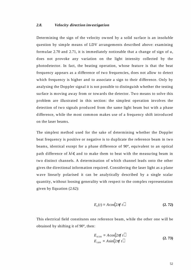
52

2.8. Velocity direction investigation

Determining the sign of the velocity owned by a solid surface is an insoluble

question by simple means of LDV arrangements described above: examining

formulae 2.70 and 2.71, it is immediately noticeable that a change of sign of u,

does not provoke any variation on the light intensity collected by the

photodetector. In fact, the beating operation, whose feature is that the beat

frequency appears as a difference of two frequencies, does not allow to detect

which frequency is higher and to associate a sign to their difference. Only by

analysing the Doppler signal it is not possible to distinguish whether the testing

surface is moving away from or towards the detector. Two means to solve this

problem are illustrated in this section: the simplest operation involves the

detection of two signals produced from the same light beam but with a phase

difference, while the most common makes use of a frequency shift introduced

on the laser beams.

The simplest method used for the sake of determining whether the Doppler

beat frequency is positive or negative is to duplicate the reference beam in two

beams, identical except for a phase difference of 90°, equivalent to an optical

path difference of λ/4, and to make them to beat with the measuring beam in

two distinct channels. A determination of which channel leads onto the other

gives the directional information required. Considering the laser light as a plane

wave linearly polarised it can be analytically described by a single scalar

quantity, without loosing generality with respect to the complex representation

given by Equation (2.62):

( )tfAtE π2cos)(0 = (2. 72)

This electrical field constitutes one reference beam, while the other one will be

obtained by shifting it of 90°, then:

( )( )tfAE

tfAE

SIN

COS

ππ

2sin

2cos

1

1

==

(2. 73)

53

The measuring beam will contain the target velocity information, in term of the

Doppler shift fD see Equation 2.65:

( )[ ]tffAE D+= π2cos2 (2. 74)

The first reference beam E1COS is directed to the first photodetector where the

beating with the measuring beam takes place. The same happens in the second

photodetector for the reference beam E1SIN. The first detector will collect a signal

due to the beating between E1COS and E2 , while the second one will collect the

beat between E1SIN and E2 , i.e.

( ) ( )[ ]( ) ( )[ ]tffAtfAEE

tffAtfAEE

DSIN

DCOS

++=+++=+

ππππ

2cos2sin

2cos2cos

21

21 (2. 75)

Plots of these two signals are shown in Figure 2.18: it is straightforward to

notice what channel is leading the other.

Figure 2. 18 Plot of the output signal from the first detector (blue) and the

output signals from the second detector (green) being fD positive

in the first picture and negative in the second one.

0 0.1 0.2 0.3 0.4 0.5

-2

-1.5

-1

-0.5

0

0.5

1

1.5

2

0 0.1 0.2 0.3 0.4 0.5

-2

-1.5

-1

-0.5

0

0.5

1

1.5

2

Time (s) Time (s)

Tim

e H

isto

ries

(V)

Tim

e H

isto

ries

(V)

54

From the previous figure it is clear that in the first case ( fD positive) the first

channel signal leads the second channel one while in the second case ( fD

negative) the opposite situation is realised.

Calculating the intensity output on the detector 1, whose sensitivity constant is

K1 , and taking into account trigonometric relationships:

( ) ( ) ( )( ) ( ) ( )( )[ ]( ) ( )( ) ( ) ( )( )

+++

+++

+=

=++++=+=

tfftftfftf

A

tfftftfftfAEEKI

DDD

DDCOS

22cos2cos2

4cos1

2

4cos1

2cos2cos22cos2cos

2

22222111

ππππππππ

(2. 76)

and neglecting high frequency components which the detector can not observe,

( )[ ]tfIKI Dπ2cos1011 += (2. 77)

A same process can be applied to the intensity recorded by the second

photodetector, of sensitivity constant K2:

( )[ ]tfIKI Dπ2sin1022 += (2. 78)

Again it can be noticed that the current variation in channel 2 leads that into

channel 1 by 90°, but if the Doppler frequency sign inverts into a negative value

the current oscillation in channel 2 becomes:

( )[ ]tfIKI Dπ2sin1022 −= (2. 79)

then it is channel 1, which leads into channel 2.

For this system to work it is indispensable that each channel receives exactly

similar samples of the scattered light which will be mixed with the reference

beams shifted in phase, in such a way that the phase difference between the

55

channels remains constant. Common optical paths for the two channels must be

used and their distinction will reside only in a different polarisation. Division of

scattered light into two channels phase-shifted is carried out in optical way, by

using a polarising beam splitter whose axes are oriented at 45° to the original

plane of polarisation of the light. Conventionally here the plane of polarisation

will be described as the plane containing the electric field and the direction of

propagation, bearing in mind that in electromagnetic theory an oscillating

electric field is always transverse to its propagation direction.

Figure 2. 19 Schematic of the optical light split and phase shift between the two

channels and the mixing of the two outputs after a second phase

shift.

It is easier to register the phase difference between the output signals from the

two diodes by mixing them: a phase shift of 90° is introduced then into the

output of one detector. The phase between the signals applied to the mixer will

then be 0° or 180°, depending on the direction of the velocity. The output of the

mixer results positive or negative according with the velocity sign. Some

smoothing of the output is needed to discriminate against noise but the

response must be rapid enough to follow the fluctuations of the tested surface

motion as closely as required.

The other method applied to remove velocity directional ambiguity is the so-

called frequency shifting technique because the reference beam or both the

reference and the measuring one undergo a change in frequency of some tens of

MHz. Only a detector is needed in this case and no modification to the optics

and signal processing should be made; an additional advantage is that it does

CHANNEL 1

INCOMINGLIGHT

CHANNEL 2

POLARISINGBEAM SPLITTER 90° PHASE

SHIFT

MIX

ER

56

not involve polarisation and, at the end, that it is suitable to follow any velocity

fluctuations smoothly through zero.

Producing a frequency shift of reference signal the initial frequency of the two

beams will differ of fS , see Equation (2.65):

( ) ( )[ ]

( ) ( )[ ]tffiA

tE

tffiA

tE

D

S

±=

+=

π

π

2exp2

2exp2

2

1

(2. 80)

The corresponding beat intensity is given by:

[ ][ ] ( )[ ] ( )[ ] tffI

tffA

EEEEI DSDS mm ππ 2cos12

2cos12

02

*2121 +=+=++=

(2.81)

where the beat frequencies are ( fS + fD ) and ( fS - fD ). This device eliminates the

ambiguity of the Doppler frequency sign making directional discrimination

possible. The use of a frequency shift greater than the Doppler shift frequency

corresponding to the maximum velocity occurring in a series of measurements

ensures that ( fS - fD ) does not change sign, enabling an unambiguous relation

between velocity and signal frequency to be obtained. Figure 2.20 shows the

spectrum of the detector intensity output: the shift frequency fD provides a

carrier frequency which is modulated from the targt surface velocity. Tracking

the frequency modulation a time-resolved analogue signal can be recorded in

both amplitude and phase.

57

Figure 2. 20 Frequency shifting and time-resolved velocity, [32].

The cheapest and straightforward technique of shifting the frequency of a laser

beam is to make it to pass through a rotating grating which diffracts the

incident light wave and makes it to emerge with a frequency change

proportional to the rotation speed by the diffraction order and the number of

lines of the grating. Tha main problem of this method is that high frequency

shifts can not be realised unless high rotational speeds are achieved, but there is

always a limit owing to vibration reasons. Then the maximum shift reachable is

5MHz.

When higher frequency shifts are requiered acousto-optic devices are

recommended. They are based upon the principle of diffraction of light by

acoustic waves that travel inside a cell the most common of which is called

Bragg cell. This device operats in the Bragg mode to yield one beam with a

frequency and direction different from the incident beam. The cell contains an

acousto-optic medium in which acoustic waves are travelling producing a

small-scale density variation. This effect generates inside the medium zones

with different refraction index and the optical beam travelling throught these

zones will be diffracted into several orders. This means that the incoming light

fS – fDfS

fS + fD

detector intensity output

time

surface velo

city

58

is divided in several beams deviated of an angle and undergone a frequency

shift proportional to the acoustic wave frequency. If the incident beam

intersects the acoustic waves at the Bragg angle the light intensity tends to be

concentrate in just one order of diffraction, specifically the first order for Quartz

media. In this way the emerging beam frequency undergoes a shift coincident

with the acoustic wave frequency. The commercially available solid medium

arrangements provide shifts around 40MHz which generally gives best results

and diffraction efficiency.

The Bragg cell introduction is usefull to avoid a further inconvinient: the

sensitivity of the system depends upon the phase shift between reference and

measuring beams, i.e. when the output intensity is maximum or zero the

sensitivity is zero. In fact that quantity is given by the intensity’s deviation

against the phase shift (that actually is the Doppler frequency):

[ ] )2sin(2

1)2cos(1

2

100 tftItfI

df

d

df

dIDD

DD

ππσ −=

+== (2. 82)

When I is maximum or zero (t = n π / fD where n = 0,1,2...I will be maximum for

even values of n and zero for odd values of n) σ is zero. Introducing a

frequency shift of fS , σ will depend on the sine of ( fS + fD ), i.e. it is never zero

although measured velocity is such.

2.9. Polytec Laser Doppler Vibrometer

Commercial LDV systems consist of two major components: the optical

sensor/controller processor and the scan control/data acquisition system. The

optical sensor contains the actual laser, the optical elements, and electrical

components needed to spatially position the laser beam. The controller

processor, containing the electronic components needed to process the velocity

information provided by the optical sensor, constitutes the interface between

59

the interferometer and the scan control/data acquisition computer. The scan

control/data acquisition system consists of the equipment and software needed

to manipulate the scan mirrors and to acquire the velocity data. In this section

only the first component will be treat, addressing the scan subject in the third

chapter.

Commercial systems nowadays available are essentially two: VPI Sensor

System manufactured by Ometron and the PSV Polytec product.

The Polytec system is a modified Mach-Zehnder interferometer (Figure 2.21),

which allow the laser beam to exit from the “inner” interferometer cell and to

hit the external target. A linearly polarised He-Ne laser is employed as a light

source, which has polarisation orientated at 45° to the horizontal plane.

Figure 2. 21 Polytec LDV arrangement.

Polytec uses as coherent light source a multi-mode (in the longitudinal

direction) Helium-Neon laser, linearly polarised with an output power between

2.2 and 3.0 mW. This fact means that there are several modes of oscillation, with

He-NeLASER

SOURCE

beam splitter3

quarterwaveplate

beam splitter1

beamsplitter 2

braggcell

measuringbeam

referencebeam

vibratingstructure

Photodetector 1

Photodetector 2

output signal

60

different wavelengths, in the laser length (longitudinal axis), while only a

transverse mode is dominant in the distribution of light across the beam and

this is the uniphase mode TEM00 (characterised by its Gaussian profile and

circular symmetry). It is important that in the transverse direction only one

mode occurs, since other transverse modes have frequencies slightly different

from the TEM00 mode and their beating may be then confused with the Doppler

signal. On the contrary the occurrence of multi-modes in the longitudinal

direction is not so critical, because they can be distinguished by their distinct

numbers of wavelengths within the laser length. In order to privilege one mode

(say the one with wavelength λ) the optical path length travelled by the wave

that is twice the cavity length (distance between the mirrors placed in the laser

oscillator system) must equal a whole number of wavelengths:

λnLc =2 (2. 83)

where Lc is the cavity length and n = 1, 2, ... .

In this case the wave passing backwards and forwards between the mirrors

reinforces itself each time around because each successive passage is in phase.

The cavity lenght in the Polytec laser head is 205 mm. In order to assure that the

same longitudinal mode will be enphasised during the travel of the laser beam

towards to and backwards from the object tested the path followed (Lp) must be

an integer multiple of the cavity length:

cp nLL = (2. 84)

wher now n = 2, 3, ... since te minimum optical path of the beam must be at least

twice the cavity length. Lp can be seen as a sort of ‘coherence repeat distance’

because is the length where the Doppler interference is maximum and the

signal output from the laser is so.

Therefore, if during the operation, a signal level minima is encountered, i.e.

fluctuations of signal level occur mostly in the course of the laser warm-up, a

61

change of the operating distance of half cavity length should resolve the

problem.

Configuration shown in Figure 2.17 is changed introducing at the place of the

actual moving target a third polarising beam splitter with a quarter wave plate

in order to realise a directional coupling: the light coming from the laser is

directed straight through the object, while the reflected beam is deflected

downwards to the second beamsplitter. The quarter wave plate is used as

optical insulator, in order to avoid that the light reflected by the target can

return towards the laser source. This optical element, also called retardation

plate, has the main characteristic to modify the polarisation of the wave

incident. In the case of quarter wave plate the polarisation direction is deviated

of λ/4, i.e. 45°. The entry beam, coming from the polariser beam splitter, see

Figure 2.22, owns a polarisation of 45° with respect to the plate axis, then it is

transformed in a circularly polarised beam inside the plate. Being reflected back

by the target surface the rotation is inverted and the travel across the plate will

transmit to the beam a polarisation of 45° but on the opposite direction. Owing

this polarisation the light can not pass again inside the beam splitter and it is

deviated downwards.

Figure 2. 22 Quarter wave plate working principle.

Therefore, a second difference with the Mach-Zehnder configuration is the

insertion of a Bragg cell as a device to discriminate the target velocity direction.

The frequency shift introduced is 40 MHz.

reflectingtarget

polarisationat 45°

polarisationat 45°

circularpolarisation

circularpolarisation

FOREWARD BEAM

BACKWARD BEAM

62

The light intensities I1 and I2 seen by the photodetectors can be derived by the

formulae written for the Mach-Zehnder interferometer - Equation (2.70) and

(2.71) - taking into account the presence of Bragg cell and then Equation (2.81).

( )[ ] tffIKI DS mπ2cos12

1011 += (2. 85)

( )[ ] tffIKI DS mπ2cos12

1022 −= (2. 86)

Both output signals from the photodetectors, which actually are photodiodes,

are converted to electrical signals. Combining them together using a differential

pre-amplifier stage the resulting output voltage is given:

( )[ ]tffKV DS += π2cos (2. 87)

where K indicated the conversion efficiency.

The voltage V constitutes the output signal of the interferometer and it is

transmitted to the processor controller where the Doppler signal is frequency

demodulated to extract the velocity information.To improve the signal quality,

affected by velocity drop-outs, the Polytec system has introduced in the

controller an optional device, which is the tracking filter2. The continuous

nature of the Doppler signal from a solid surface measurement allows

frequency tracking demodulation. To obtain real time demodulation of

photodetector signal giving voltage proportional to instantaneous velocity

component a tracking filter is activated instead of using a conventional

spectrum analyzer. The tracking scheme is applying the principle of PLL (phase

locked loop), where a Voltage-Controlled Oscillator (VCO), controlled via the

feedback loop, tracks the incoming Doppler signal. A mixer at the input stage

2 The frequency tracker allows demodulating the Doppler-signal in order to clean the signal itself from drop-outs. Therefore, it does not enhance signal qualityitself. The demodulator must be designed in such a way that it is able to distinguish between a signal drop-out and a vibration’s low level when the signaldisappears.

63

produces an “error” signal between the Doppler and VCO frequencies which is

band-pass filtered and weighted before being integrated and used to control the

oscillator to drive the error to a minimum. The feedback loop has an associated

“slew rate” which limits the frequency response of the processor. The overall

effect of the tracker is to act as a low pass filter, which output the VCO voltage

as a time, resolved voltage analogue of the changing frequency. The frequency

range of interest for most vibration measurements is well within the range of

this form of frequency demodulation. The tracker incorporates weighting

networks, which tailor the control of the VCO according to the signal to noise

ratios of the incoming signal. The network will hold the last value of Doppler

frequency being tracked if the amplitude of the signal drops below a pre-set

level. In this way the Doppler signal effectively drops out and careful

consideration must be given to the statistics of what is essentially a sampled

output, especially when high frequency information of the order of a dropout

period is required. Fortunately for most practical applications this period,

typically 0.2 µs, is negligible.

At last another option provided within the Polytec LDV is the auxiliary filter,

which is applied to the force-signal to compensate for filter gain and phase-

shifts. No such compensation is available in anyone else commercial instrument

2.10. Ometron Laser Doppler Vibrometer

The operating principle is based on the Michelson interferometer technique

with the only difference constituted by the introduction of a device to eliminate

the ambiguity on the velocity direction of the structural motion along the laser

line-of-sight. In the VPI sensor this is done by frequency shifting the frequency-

coded velocity information and the shift is accomplished by electronic mixing:

the recombined beam is split into two detection channels which are optically

configured in such a way that one channel receives interferometric modulation

that is effectively shifted by one-quarter wavelength (2π/4 = π/2 = 90°) relative

to the other channel. This results in a 90° phase shift between the channels,

64

which are denoted as “sin” and “cos”. The direction of motion is then

determined by which signal phasewise leads the other. Schematic of the VPI

Sensor unit is shown in Figure 2.23.

Light emitted by the source reaches the first beam splitter that splits it in two

beams of same amplitude, ideally. The first beam ① goes on towards a fixed

target (reference beam) while the second ② is deflected to the vibrating

structure (measuring beam). Then they are back reflected from the surfaces they

hit and they are recombined in the same beam splitter.

Figure 2. 23 Ometron VPI configuration.

Being the electric field produced by the laser source A exp (-iωt) , after the split

the two fields would have the same amplitude ½ A . Because they follow

different path, say the one towards the fixed target takes a time as Tr , while the

one towards the vibrating object Tr + Tm (Tm is named the time delay associated

to the measuring beam), the fields in ① and in ② would have the following

expression respectively:

SSBSCDoppler 1 Doppler 2AnalogVelocity

BALANCEDMODULATOR

FM

VIBRATINGSTRUCTURE

MEASURINGBEAM

REFERENCEBEAM

BEAMSPLITTER

He-NeLASER

SOURCE

¼ wavelengthBEAM SPLITTER

COS

SIN2 3

5

41

FIXED MIRROR

65

( ) ( )

( ) ( )[ ]mrm

rr

TTitiAE

TitiAE

+=

=

ωω

ωω

expexp2

1

expexp2

1

(2. 88)

After recombination ③ the field detected by the sensor is

( ) ( ) ( ) ( )[ ]

( ) ( ) ( )[ ]mr

mrrf

TiTitiA

TTitiATitiAE

ωωω

ωωωω

exp1expexp2

1

expexp2

1expexp

2

1

+=

=++=(2. 89)

where exp ( iωTr ) is a constant depending on the construction specifications of

the optical components and ωTm is the optical path difference between the

reference beam and the measuring one. If the path covered by the measuring

beam to shot the vibrating structure is larger than the one followed by the

reference beam to reach the fixed object and the difference is z , the

comprehensive distance would be 2z (for and backward). Then

λπ

λπω z

c

zcTm

422 == (2. 90)

being ω the light frequency (2π c/ λ ) , λ its wavelength and c the light velocity.

Besides Tm is the time the light needs to cover the distance 2z , being its speed c.

The distance z will depend upon the velocity of the vibrating object in the

straightforward way: z = v t. This leads to the final expression:

tftv

tvz

T Dm πλ

πλπ

λπω 2

22

44 ==== (2. 91)

where the Doppler frequency is easily recognizable fD = 2v / λ .

Substituting this value in the electric field formulation:

66

( ) ( ) ( )[ ]tfiTfitfiAE Drf πππ 2exp12exp2exp2

1 += (2.92)

which is the electric field at position ③ .

If the photodetector is placed at this point (without having any shift of the

beam) the intensity that will be decoded is:

( ) ( ) ( )[ ]

( ) ( ) ( )[ ]

( ) ( )[ ]12exp2exp14

1

2exp12exp2exp2

1

2exp12exp2exp2

1

2

*

+−++=

=

−+−−×

+==

tfitfiA

tfiTfitfiA

tfiTfitfiAEEI

DD

Dr

Drff

ππ

πππ

πππ

(2. 93)

From the Euler formulae the measured intensity expression can be simplified

as:

( )[ ] ( )[ ]tfItfAI DD ππ 2cos12

12cos22

4

10

2 +=+= (2. 94)

being I0 the intensity of the initial field. The intensity of the electrical field

measured is not sensitive to the sign of velocity, which does not produce

difference in frequency. The technique used here for the discrimination of the

velocity direction is the shifting the frequency of light beams.

The recombined beams are duplicated in two channels, identical except for a

phase difference of 90° equivalent to an optical path difference of λ/4,

introduced into one of the beams. A determination of which channel leads onto

the other gives the directional information required. This mode of operation is

similar to the working principle of frequency trackers manufactured by

Cambridge Consultants and by Communications and Electronics Ltd., [32]. The

67

photodetector signal (in this case Ef at position ③) is divided and mixed

separately with two components of a Voltage Control Oscillator (VCO), which

produce two outputs at the frequency f having a 90° phase relationship with

each other. The two mixed signals are low-pass filtered to remove the high

frequency components.

Calling the fields in the two channels ESIN and ECOS they would result from the

mix of the photodetector signal Ef and the outputs form the VCO.

( ) ( ) ( )[ ]

( ) ( ) ( )[ ] )2cos(2exp12exp2exp4

1

)2sin(2exp12exp2exp4

1

tftfiTfitfiAE

tftfiTfitfiAE

DrCOS

DrSIN

ππππ

ππππ

+=

+=(2.95)

Using the generalised Euler formula:

( ) ( ) ( )[ ] ( ) ( )[ ]

( ) ( ) ( )[ ] ( ) ( )[ ]tfitfitfiTfitfiAE

tfitfitfiTfitfiAi

E

DrCOS

DrSIN

πππππ

πππππ

2exp2exp2exp12exp2exp8

1

2exp2exp2exp12exp2exp8

1

−++=

−−+=

(2. 96)

Multiplying and filtering out the high frequency component:

( ) ( )[ ]

( ) ( )[ ]tfiTfiAE

tfiTfiAiE

DrCOS

DrSIN

ππ

ππ

2exp12exp8

1

2exp12exp8

1

+=

+=(2. 97)

This two signals are called Doppler 1 and Doppler 2 and can be derived as

output from the VPI sensor. Observing their plots in Figure 2.24 it is

straightforeward to notice what channel is leading the other.

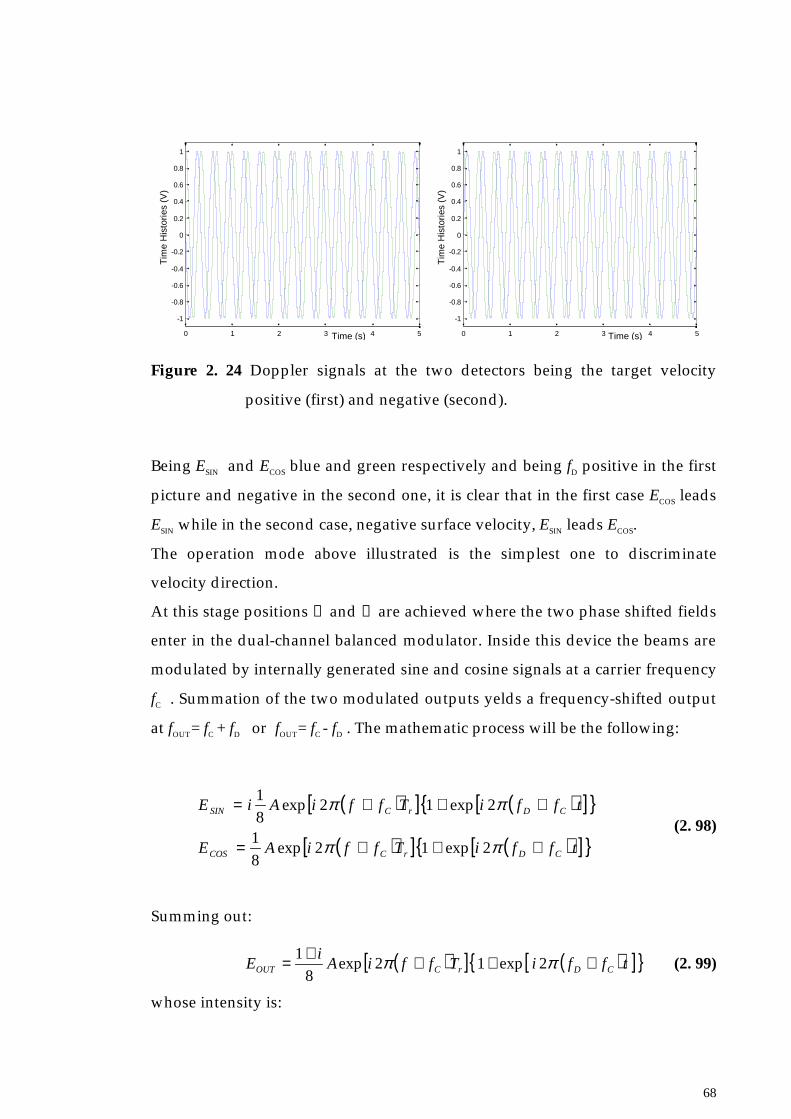
68

Figure 2. 24 Doppler signals at the two detectors being the target velocity

positive (first) and negative (second).

Being ESIN and ECOS blue and green respectively and being fD positive in the first

picture and negative in the second one, it is clear that in the first case ECOS leads

ESIN while in the second case, negative surface velocity, ESIN leads ECOS.

The operation mode above illustrated is the simplest one to discriminate

velocity direction.

At this stage positions ④ and ⑤ are achieved where the two phase shifted fields

enter in the dual-channel balanced modulator. Inside this device the beams are

modulated by internally generated sine and cosine signals at a carrier frequency

fC . Summation of the two modulated outputs yelds a frequency-shifted output

at fOUT= fC + fD or fOUT= fC - fD . The mathematic process will be the following:

( )[ ] ( )[ ]

( )[ ] ( )[ ] tffiTffiAE

tffiTffiAiE

CDrCCOS

CDrCSIN

+++=

+++=

ππ

ππ

2exp12exp8

1

2exp12exp8

1

(2. 98)

Summing out:

( )[ ] ( )[ ] tffiTffiAi

E CDrCOUT ++++= ππ 2exp12exp8

1(2. 99)

whose intensity is:

0 1 2 3 4 5

-1

-0.8

-0.6

-0.4

-0.2

0

0.2

0.4

0.6

0.8

1

0 1 2 3 4 5

-1

-0.8

-0.6

-0.4

-0.2

0

0.2

0.4

0.6

0.8

1

Tim

e H

isto

ries

(V)

Tim

e H

isto

ries

(V)

Time (s) Time (s)

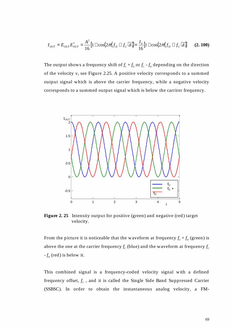
69

( )( )[ ] ( )( )[ ]tffI

tffA

EEI CDCDOUTOUTOUT ++=++== ππ 2cos116

2cos116

02

* (2. 100)

The output shows a frequency shift of fC + fD or fC - fD depending on the direction

of the velocity v, see Figure 2.25. A positive velocity corresponds to a summed

output signal which is above the carrier frequency, while a negative velocity

corresponds to a summed output signal which is below the carrirer frequency.

Figure 2. 25 Intensity output for positive (green) and negative (red) targetvelocity.

From the picture it is noticeable that the waveform at frequency fC + fD (green) is

above the one at the carrier frequency fC (blue) and the waveform at frequency fC

- fD (red) is below it.

This combined signal is a frequency-coded velocity signal with a defined

frequency offset, fC , and it is called the Single Side Band Suppressed Carrier

(SSBSC). In order to obtain the instantaneous analog velocity, a FM-

0 1 2 3 4 5

-0.5

0

0.5

1

1.5

2

ωC

ωC+ωDωC-ωD

IOUT

t

fCfC +

fD

70

demodulation circuit is employed. Instantaneous signals available to the user

are: Doppler 1, Doppler 2, Analog Velocity and the SSBSC.

In the VPI Sensor the device where the analog velocity waveform is derived

from the Doppler signal is a modulator-demodulator circuit which, as described

in the manual, require that the Doppler signal exceeds an amplitude threshold

(300 to 400 mV pk-pk referred to the external Doppler monitor sockets). Below

this value the velocity output will be dropped to zero or to a value less than

reality and this effect is the so-called dropout. As already stated, causes of

dropouts are: operation in between optimum distances, using a test surface

with poor reflectivity, misfocus of the measuring beam or operation at an

incorrect range.

2.11. Conclusions

This chapter has focused on a description of laser Doppler vibrometry with its

fundamental principles (i.e. Doppler effect and laser light).

Considerable emphasis has been given to an investigation into the main

problem affecting the measurement techniques, using coherent light as velocity

detector, which is the “speckle noise”. Section 2.4 is entirely devoted to the laser

speckle explaination as it can be found in literature, while Section 2.5 presents

the well-known effect of the speckle which can be seen also in the experimental

work done throughout this work (Chapters 5 and 7) and that is the frequency

broadening of the LDV output spectrum. Starting from the work done by T.

Asakura and N. Takai, [30], the treatement of the subject has been expanded in

order to lighten the dependence of the phenomenon on some parameters which

can be controlled during the experiment. In fact, it can be concluded that the

most significant factor influencing the speckle noise is the laser beam width at

its intersection with the tested object surface, which can be governed by

focusing the laser spot on the structure. Morever, the investigation has been

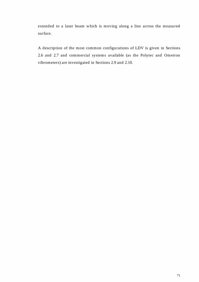
71

extended to a laser beam which is moving along a line across the measured

surface.

A description of the most common configurations of LDV is given in Sections

2.6 and 2.7 and commercial systems available (as the Polytec and Ometron

vibrometers) are investigated in Sections 2.9 and 2.10.

Chapter 3 SLDV Theory

3.1. Introduction

The main purpose of this thesis is to investigate the continuous LDV scanning

method of measuring vibration in all its facets, involving the short scan

performance (to recover simultaneously the vibration responses in different

directions at one point, see Chapter 4) and the long scan technique (to derive

the operating deflection shape of a line or a surface where the scan is

performed, see Chapter 5). In order to have a basis for comparison of the long

scan method, the traditional point-by-point scanning technique was taken into

consideration.

A definition of point-by-point and continuous scan would be helpful in

understanding the difference between the two techniques. The point-by-point

scan, also called “scanning technique at discrete points” or, simply, discrete or

traditional scanning, is a way to measure the vibration velocity of a whole

surface by measuring at a series of points, the geometric grid, on the surface

itself. The overall measurement consists of a series of vibration responses

(generally FRFs) obtained at each single point on the grid. The measurement

73

procedure starts with the laser beam pointing at the first point on the grid

where the acquisition of the vibration response takes place. When the

acquisition is finished, the laser beam moves to the next point and acquisition of

the FRF at the second point starts. The procedure automatically carries on until

the response at the last point on the grid is acquired. The test can be performed

with different kinds of excitation, i.e. sine, broad-band or random excitation.

The continuous scanning technique is a method to measure the vibration

velocity of a surface by sweeping it with a laser beam scanning continuously

over the surface. Ideally, all the points constituting the surface will then be

addressed, and a complete cycle of scan (in which the whole area is travelled)

would be sufficient to reconstruct the operating deflection shape. During the

scan, which can take few seconds, the acquisition of the time history measured

by the moving laser beam is performed. From the time signal the Fourier

coefficients can be recovered and transformed into polynomial coefficients

describing the shape of the surface’s vibration response. These data only are

needed for the analysis; therefore a very small amount of data must be stored,

depending on the order of the polynomial. From the recorded polynomial

coefficients the spatial ODS of the tested surface is reconstructed with an

arbitrary spatial resolution completely independent from the performed

measurement. This is an important advantage of the continuous scanning

technique, together with the small amount of stored data and the short

acquisition time. In fact with the point-by-point scanning technique the spatial

resolution defining the ODS derive from the number of points actually

measured. Consequently, increasing the spatial resolution implies a larger

amount of data to be recorded and a lengthening of the acquisition time. The

continuous scanning tests described in this thesis involve mono-frequency sine

excitations only and step-sine excitations when a range of frequencies is needed

for the vibration analysis, which can become more time-consuming. However,

continuous scanning techniques have been applied in structure excited with

different kind of excitations as impact, see references [33] and [14], narrow-

band, see references [3] and [8], and broad-band multi-sine excitation, [34].

74

In this chapter, the traditional scanning technique is addressed in order to

better understand its features, since in the next chapters (specifically in Chapter

5 and in Chapter 7, with regards to the applications of the continuous scanning

methods) the results of the point-by-point technique will be used for

comparison with the results derived from the continuous scanning techniques.

3.2. Basics of SLDV technology

Scanning Laser Doppler Vibrometry technology consists of an LDV with two

moving mirrors, driven by galvanometric actuators. This technique allows us to

measure accurately, from a remote position, selected point velocities where the

laser beam can be directed automatically. Such an instrument can perform a

series of velocity measurements across a grid of points defined over the surface

under test, providing reductions in the time needed to carry out vibration tests,

in contrast to traditional methods involving conventional transducers (i.e.

accelerometers).

The first prototype of an SLDV was assembled by Dr. Stoffregen and Felske

from Volkswagen AG in Germany, in 1981. They built a data acquisition and

processing system which was used to drive the laser beam emitting from a

conventional Laser Doppler sensor and process its velocity output. Moreover,

their system was supplied with an integral video camera which monitored the

location of the laser beam on the test item. The main advantage was that the

measured results could be overlaid on an image of the tested surface itself. This

design was found to be a significant help for SLDV applications and,

consequently, it has been adopted by most manufacturers of Laser Doppler

Vibrometers.

The system consists of a Laser Doppler sensor head, which performs the

velocity measurement, and two galvanometer scanners that aim the laser beam

at the pre-defined measurement position in two-dimensional space. Such a

75

vibrometer, which is now able to drive the beam by means of the two

galvanometer motors, is controlled by a specialised computer hardware and

software that complete the SLDV system. The computer drives the beam to

scan, pauses for the time needed to take the measurement at each acquisition

point, gathers signals proportional to velocity of the particular measurement

point relative to a reference, and averages these signals, if necessary. The

galvanometer-driven mirrors are then repositioned and data for the next

measurement point are acquired. The data acquisition system includes an

analogue-to-digital converter, which collects the analogue output voltage of the

laser sensor and stores it in a digital manner in order to process it later. The

result, obtained by video processing the acquired signals, is a bit-map of the

velocity data for the entire scan area with a resolution which is determined by

the user within the maximum range of the system (512 × 512 measurement

points for Polytec systems). Software is used to control the sensor and to

display the measurements in a variety of formats.

3.3. Scanning mirror system

The scanning operation is performed by leading the laser beam emitting from

the source towards two moving mirrors, which serve to aim the measuring

beam at the specified location on the test surface, see Figure 3.1. The mirrors are

driven by two galvanometer actuators: by applying a voltage to each of them,

the mirrors will rotate about their axes of two angles related to the voltages by

some constants defined via a prior calibration of the scanning system. Calling

the voltages supplied to the horizontal mirror and the vertical one, Vx and Vy

respectively, the mirrors’ rotation angles (indicated as αx and αy) will be

described by the following relationship:

yy

xx

VS

VS

==

αα

(3. 1)

76

S being the galvanometer static sensitivity (4 º/V from the manufacturer

specifications), [35].

Figure 3. 1 Schematic representation of the mirrors rotation.

The scanning angles, αx and αy, can be decided by software and used as inputs

for the scanner control which is basically an interface between the data

acquisition/processing computer and the mirror driver motors, constituting of

a digital-to-analogue converter (DAC). This transforms the digital value of the

angles to voltages. The latter are applied to the galvanometer actuators to give

the specific rotation to the mirrors and to deflect the laser beam to the sought

position on the test item. The galvanometer scanner not only consists of the

mirror and the actuator, but two further components are included in the device:

a built-in capacitive rotation sensor to measure the actual angular shaft position

of the mirror and a PID (Proportional, Integrative, Derivative) control system to

generate a feedback control signal. This means that the galvanometers work

within a closed loop control, as shown in the flow-chart illustrated in Figure 3.2,

which allows it to determine precisely the spatial relationship between the test

Vy

Vx

αy

αxbeam out of thescanner system laser beam to the

scanner system

y-mirror

x-mirror

77

structure and the SLDV system. It then accurately positions the laser beam on

the desired location, [36].

Figure 3. 2 Flow-chart of the feedback control action.

The dynamic performance of the scanner system is related to the rotor and

mirror inertias, actuator torque and PID control algorithm. Step response time

depends on torque to inertia ratio and PID parameters. Mirror dimensions

should be chosen as a compromise between the need for a large optical aperture

for the scanning, and mirror inertia, in order to have a fast response of the

mirror itself.

A typical optical scanner used by the SLDV manufacturers is model G325DT

from General Scanning Inc., whose common performance is reported in Table

3.1 and 3.2, [37].

angle fromsoftware

PID control

galvanometermotor

capacitivesensor

measuredangle

78

Mirror

Useable aperture. 20 mmMirror+Mount Inertia. 6.5 g- cm2

‘L’ Dimension. 29 mm‘H’ Dimension. 37 mm

Table 3. 1 Characteriscs of mirrors employed in low-inertia scanners.

Optical Scanner

ParametersNominal accuracy of the

motor/driver unit. 0.01 deg / 0.175 mrad.Specified scan resolution. 0.0025 deg / 0.045 mradPointing stability. typ. 0.0035 deg / 0.06 rad

(after 1 hour warm-up over a period of 25

Position repeatability. typ. 0.001 deg / 0.018 rad

Table 3. 2 Performance of galvanometer scanners.

At present, the SLDV is only applied to displace a laser beam on a static grid of

points, by driving the motors with discrete analogue voltages, which change

point by point. The measurement acquisition is done for each point

subsequently and only starts when the mirrors have come to rest. Because the

galvanometer scanners are supplied by direct current, it is possible to drive

them by voltages which vary continuously in order to make the laser beam

follow a pre-determined trajectory and perform the so-called continuous

scanning.

L

H

79

3.4. Polytec Discrete Scanning Utility

SLDVs consist of a single point laser Doppler vibrometer, a scan unit and a data

processing/management system.

The heart of the system is the optical sensor head (OFV-055) which consists of a

single-point interferometer which focuses the laser beam towards the x-y

scanner mirrors driven by the scanner driver electronics. Further, a compact

video camera is installed on the case of the head for the visual observation of

the test item and the scanning procedure. In fact, by means of a video control

box settled on the PSV computer, the grid of measurement points to be

followed over the structure surface is defined on top of the video image

displayed on the computer monitor. In order to perform a correct measurement,

the laser beam must be aligned to the video image and this is done by a

calibration routine included in the Polytec software (PSV-200). This routine

automatically corrects parallax errors and distortions to allow accurate

positioning of the beam. In conjunction with the optical head there is the

electronic signal processor/controller unit (OFV-3001-S) which controls the

measuring parameters and processes the output of the laser sensor in order to

derive the velocity information.

3.5. Speckle Noise and its Improvement by the Exploitation of

Commercial Devices (Tracking filter and Signal Enhancement

Facility)

Since speckle noise is an intrinsic physical effect linked to coherent light

backscattered from an optical rough surface, its occurrence cannot be avoided.

As seen in Chapter 2, it appears on the LDV signal as dropouts, i.e. sudden

drops in the laser light intensity, which deteriorates the signal, reducing the

accuracy of measurement.

The tracking filter is a device based on the PLL (Phase Locked Loop) principle

and it is used to bypass the signal losses owing to dropouts. At its heart is a

80

Voltage Controlled Oscillator whose output variations are the same as the

Doppler signal (i.e. it is locked to the signal). When a dropout occurs in the

signal intensity, the tracker freezes the frequency of the Voltage Controlled

Oscillator during the dropout period, then, as the signal reappears, it locks in

again to the signal. The tracker behaves as a “flywheel” that follows the signal

and holds its intensity as it was before the intermittence of a dropout occurs.

The device only works properly if the measurement area does not undergo

excessive accelerations, which are the product of frequency and velocity of the

surface vibration. Also, the losses of signal should not be too long, i.e. the signal

amplitude reduction is only limited to a small number of samples. The latter is

always realised in the case of the measurement of solid surface vibration by

using a steady laser beam as a sensor. Alternatively, when the beam is

sweeping across a vibrating surface (case of continuous scanning technique),

the output signal amplitude is modulated by the deflection shape of the surface

itself. When the beam is passing through areas which undergo a low vibration

level, the amplitude of the time signal will reduce to lower values and the

tracking filter will cease to work. In conclusion, the tracking filter is unhelpful

in the case of continuous scans.

An additional option incorporated in Polytec SLDV systems is the Signal

Enhancement system, a sophisticated routine which can improve data quality.

The most important cause of speckle noise is the change of speckle pattern

received by the detector during the measurement time. This change is strictly

related to the relative motion between tested structure and laser beam, usually a

sideways motion perpendicular to the laser line of sight. This occurrence is

practically unavoidable when the structure is vibrating because the laser spot

cannot be kept completely fixed at the specific position. With the Signal

Enhancement device activated the PSV software estimates the SNR of the actual

measured signal and, if this parameter is below a certain threshold level, the

laser beam is moved slightly from its position and the measurement taken

again. The measurement procedure can be repeated up to seven times at

different points around the actual measurement point chosen within the

81

geometric grid. By performing a weighting average of the measured data at the

different positions, the acquired signal quality is optimised, the only

disadvantage being an increase in measurement time.

Because this algorithm is incorporated in the PSV Software which can be used

exclusively in the fixed position mode of operation it is not possible to take

advantage of it, when a continuous scan is performed. However, its philosophy

could be applied to the continuous scanning technique by performing several

scans along, say, different lines which are slightly apart from each other and by

making an average of the signals acquired.

3.6. Vibration Measurements by Discrete Scanning

Two-dimensional vibration Operating Deflection Shapes (ODSs) of structures

can be derived by measuring FRFs on a grid of points selected over the test

structure. The measurement philosophy is the same as that which uses

accelerometers moved across the grid. The evident advantage is the use of a

non-contact transducer, as in a laser sensor, and the automation of the

measurement technique together with the time saving that can be achieved.

In order to understand the application of the point-by-point technique, an

experiment was performed on a simple steel rectangular plate, 174 × 199 mm,

cantilevered at one edge and excited in a range of frequencies between 0 and

2 kHz, using a pseudo-random excitation via an electromagnetic shaker

attached off-centre on the structure, as shown in Figure 3.3. The same structure

will be employed to test the continuous scanning method for deriving ODSs, as

will be shown in Chapter 5.

82

Figure 3. 3 Experimental configuration.

The laser was made to scan step by step over a grid of 546 points (see Figure

3.4).

Figure 3. 4 Measurement points grid.

The velocity range set for the velocity decoder was 125 mm/s/V which

represents the scale factor between the actual point velocity and the vibrometer

output voltage.

SHAKER

PLATE

CONSTRAINT

POINT A

POINT B

83

The acquisition was performed by activating the tracking filter and the ‘Signal

Enhancement’ routine to improve the signal quality. Furthermore, a third

option was selected via software: the so-called ‘Remeasure’ option whose

purpose is to reject measurement points which do not have a valid status (i.e.

during the acquisition there was an over-range or the signal level was low) and

to remeasure again in the same location until the signal quality is acceptable.

‘Signal Enhancement’ and ‘Remeasure’ routines have the sole disadvantage of

increasing the acquisition time of the test but it is worth using them to achieve

good output signals for most of the points on the grid. In order to minimise the

noise level, averages were also performed; in the experiment included here five

averagings were found to be sufficient to obtain the optimal output signals.

Vibrometer output signals and reference signals, acquired from a force

transducer attached to the plate, were measured at each point with an anti-

aliasing low-pass filter activated. The analogue signal had to be sampled for a

certain amount of time with a suitable sampling frequency, namely 2.56 times

bigger than the frequency bandwidth chosen for the measurement (2 kHz). The

number of samples which the analogue signal will be cut into are defined,

again, as 2.56 times the FFT lines set in the PSV data acquisition (6400 lines in

the actual experiment). From these data the time required to measure the

velocity at one point could be calculated as:

sfrequencysample

samplesofnumberwindowtime 2.3

56.22000

56.26400 =⋅⋅==

An important parameter, which is a comparison term between discrete and

continuous scans across an area, is the total time necessary for the test to be

completed. For an area scan, the total measurement time can be derived as the

following product:

hoursaveragingsofnpointstmeasuremenofnwindowtimetimetotal 43.255462.3.. =⋅⋅=××=

84

In reality, together with this ideal quantity, additional times must be

considered:

- time required for remeasuring measurement points which do not have a

valid status;

- time necessary for waiting until the scanner mirror is at rest, which is set

by default at 10 ms. The so-called settling time must be greatly

emphasised as the mirrors should be in a stable position before the

measurement starts, otherwise the laser spot on the structure will not be

steady on the selected measurement point and the relative motion

between laser beam and tested surface will produce speckle pattern

motions with consequential dropouts.

The measurement time will increase further if additional facilities for signal

quality improvement (i.e. signal enhancement) are selected. The total

acquisition time for the actual test (564 points) was in excess of 4 hours.

The further parameter used to compare discrete and continuous scanning

techniques is the ODS representation resolution, which coincides with the

number of grid points in the fixed position mode of operation. In the test

performed here, the geometry grid resolution consisted of 546 measurement

points.

During the acquisition, an on-line processing of the data could be carried out. In

the PSV software FRFs were stored for each point on the grid. They were

derived at each measurement point by dividing the Fourier spectrum of the

vibrometer output, at the actual acquisition point, by the reference signal,

taking into account the averages. Since the quantity measured by the laser is a

velocity, the resulting FRF will be a mobility, estimated with averaged

measurement values (H1 estimator), i.e. output noise on vibrometer channel is

suppressed. The transfer mobility between the measurement point A and the

excitation point B, illustrated in Figure 3.4, is shown in Figure 3.5.

85

0 200 400 600 800 1000 1200 1400 1600 1800 2000-50

0

50

Mag

nitu

de (d

B -

0 dB

= 0

.025

m/s

/N)

0 200 400 600 800 1000 1200 1400 1600 1800 2000-200

0

200

400

Frequency (Hz)

Pha

se (d

eg)

Figure 3. 5 Transfer mobility at point A.

After the area scan had taken place, FRFs for all valid measurement points

would be saved in order to be post-processed by using the standard PSV200

presentation module. Velocity maps for each resonance frequency chosen

within the average spectrum of all grid points could be displayed. These

patterns could be seen as ODSs at the selected frequency. Modal analysis was

not performed on the data acquired, and therefore it is not appropriate to use

the expression of “mode shapes”. Two frequencies were selected: 181.9 Hz (4th

resonance) and 239.1 Hz (5th resonance). ODSs at the same frequencies will be

derived with the continuous scan operation mode in Chapter 5.

Values of instantaneous velocity at each measurement point are shown in

Figures 3.6 and 3.7, plotted against the x and y coordinates of the points in a 3-D

reference system.

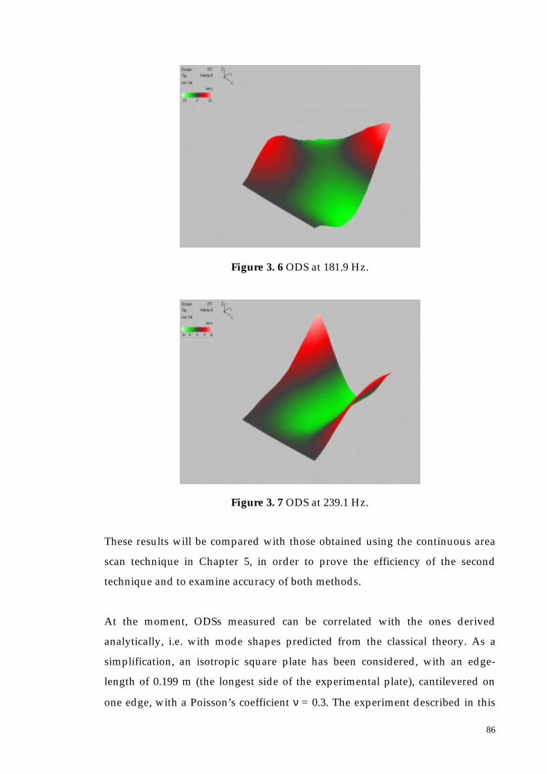
86

Figure 3. 6 ODS at 181.9 Hz.


These results will be compared with those obtained using the continuous area

scan technique in Chapter 5, in order to prove the efficiency of the second

technique and to examine accuracy of both methods.

At the moment, ODSs measured can be correlated with the ones derived

analytically, i.e. with mode shapes predicted from the classical theory. As a

simplification, an isotropic square plate has been considered, with an edge-

length of 0.199 m (the longest side of the experimental plate), cantilevered on

one edge, with a Poisson’s coefficient ν = 0.3. The experiment described in this

87

chapter was done in a different moment of the one described in Chapter 5, in

fact it can be noticed that the clamping conditions are different, specifically here

the plate was deeper-clamped (its length is 0.199 mm while in the experiment in

Chapter 5 the length is 0.244 mm). The analytical calculation was, then, made

with different parameters. The resonance frequencies changes as well, even if

slightly: 181.9 Hz and 239.1 Hz instead of 202.4 Hz and 242.68 Hz (see Section

5.5.4.2). The mode shapes are given by:

( )

+−−

+−++

−+= ∑ ∑

= =

l

y

l

x

l

x

l

x

l

y

l

y

l

y

l

yA

l

yAAyxW

mmm

mm

p

m

q

n

nnn

nnmnmm

εεαεε

εεαεε

sinsinhcoscosh

sinsinhcoscosh213,1 3

21 (3. 2)

where l is the plate dimension, Amn , αm, εm, αn, εn, are coefficients whose values

are given in Table 4.45 and 4.46 in reference [38]. Representations of mode 4 and

mode 5 are easily found numerically, using the same grid of coordinates (x, y)

applied for the plots of the mode shapes derived experimentally by Discrete

Area Scan.

Figure 3.8 and 3.9 show theoretical and experimental area-scan ODSs for the

two frequencies analysed.

Figure 3. 8 ODS at 181.9 Hz (4th Mode).

88

Figure 3. 9 ODS at 239.1 Hz (5th Mode).

For both modes, theoretical and PSV ODSs can be plotted together to emphasise

the areas on the plate where the measured data do not follow the prediction.

This is done in Figure 3.10.

Figure 3. 10 Measured and theoretical ODSs overlaid for mode 4th (left) and

mode 5th (right).

The maximum shift between the two sets of data is concentrated on the free-end

of the plate and on the right-side of the cantilevered end. The latter means that

the constraint is not perfectly realised.

89

3.7. Fast Scan Option

The Fast Scan procedure measures in a narrow band frequency only, centered

on the frequency selected. The frequency bandwidth can be chosen also and

will coincide with the bandpass filter bandwidth employed for acquisition.

Because Fast Scan aims to speed-up the measurement process, the options

‘Averagings’ and ‘Signal Enhancement’ are disabled.

With this capability activated, speeds up to 100 discrete points/sec can be

achieved.

In the PSV200 Presentation Mode there is no longer any need to select a

frequency band as the ODS at the central frequency will automatically be

displayed.

Acquisitions had been performed in this mode of operation by choosing center

frequencies close to the ones analysed in the previous section and a bandwidth

of 20 Hz, in such a way to be sure to include the resonance frequency. The first

scan was done at 185 Hz and the second one at 237 Hz. Measurement

parameters had been kept unchanged, i.e. the number of points on the grid is

still 546. Total time needed for the complete acquisition was 3 min and 30 sec

for the first scan and 2 min and 28 sec for the second one. Time had been

stretched because the option ‘Remeasure all invalid points’ was activated.

ODSs derived in the frequency bandwidth measured were displayed

automatically by opening Presentation Mode and they are shown in Figure 3.11

and 3.12. Note that they completely reproduce the ODS recovered by the

conventional Discrete Area Scan (Figure 3.6 and 3.7).

90



3.8. Conclusions

In summary, this chapter’s aim has been to describe the use of a commercially

available system, such as the Polytec scanning vibrometer, which is able to

measure operating deflection shapes of 3D structures. The system has been

employed to perform a vibration measurement on a test piece, such as a simple

plate, and the results obtained were compared with the ones obtained using the

91

continuous scanning technique as will be shown in the following Chapters of

this thesis.

Some early conclusions about the differences between the two techniques, i.e.

the point-by-point and the continuous scanning ones, can be drawn. The point-

by-point scanning technique is more time-consuming because measurements

must be made at a large number of points in order to have enough spatial

resolution, while in the continuous scanning technique the spatial resolution

used for the representation of the polynomial deflection shape is completely

independent of the acquisition. However the continuous scanning technique is

suitable with sine excitations only, at least as far as the work done in this thesis

is concerned. In this case we must compare the results with the ones obtained

by using the fast scan option included in the Polytec system, where the

measurement is performed at one frequency and the acquisition is greatly

speeded up (i.e. it could take seconds as the continuous technique does).

However, the spatial resolution of the recovered ODS always depends on the

geometric grid and an increase of the measurement points will slow down the

measurement itself, while the ODS derived by the continuous scanning

technique can be represented with an arbitrary resolution, indeed.

Chapter 4 Continuous Scanning TechniqueApplied on MDOF VibrationResponse Measurements

4.1. Measurement Methodology

Continuous Scanning Laser Doppler Vibrometry (CSLDV) is a further feature of

the scanning methodology applied to an optical sensor as a laser vibrometer,

with its intrinsic advantage of being non-contacting and non-invasive. The

philosophy of measuring vibration response of a structure by moving the

measurement position continuously across its surface can be applied with any

transducer, with the possibility to find in the future a sensor not sensitive to the

speckle noise which is the main disadvantage affecting laser vibrometers, see

references [8], [9], and [20]. Continuous scans can be made in different ways as

mentioned in Section 3.2, by driving the x, y, beam-deflection mirrors in the

LDV head with analog signals. A classification of the different trajectories the

laser beam can be made to follow is outlined in Tables 4.1 and 4.2. A first

distinction between them can be made in terms of long and short scan lengths,

i.e. large or small amplitudes of the waveforms applied to the mirrors.

93

MIRROR DRIVER SIGNALS SCAN TYPE APPLICATION

One sinewave or

triangular wave

Line scan • One-dimensional

structures (beams)

• Raster scans across a

plate

Two sinewaves at the

same frequency

Circular scan 2-D structures:

Circular scan on a plate

or a disc

Two sinewaves at

different frequencies not

fractionally related

Area scan

(Lissajous

trajectory)

2-D structures (plates)

Two triangular waves at

different frequencies not

fractionally related

Area scan 2-D structures (plates)

A triangular wave and a

sinewave at different

frequencies not

fractionally related in

polar coordinates

Circular area

scan

2-D structures (discs)

Table 4. 1 Long scans.

MIRROR DRIVER SIGNALS SCAN TYPE APPLICATION

One sinewave Line scan Point measurement:

Translational and one

angular vibration

recovering

Two sinewaves at the

same frequency

• Circular

scan

• Conical

scan

Point measurement:

• Translational and

two angular

vibrations

• Three translational

vibrations

Table 4. 2 Short scans.

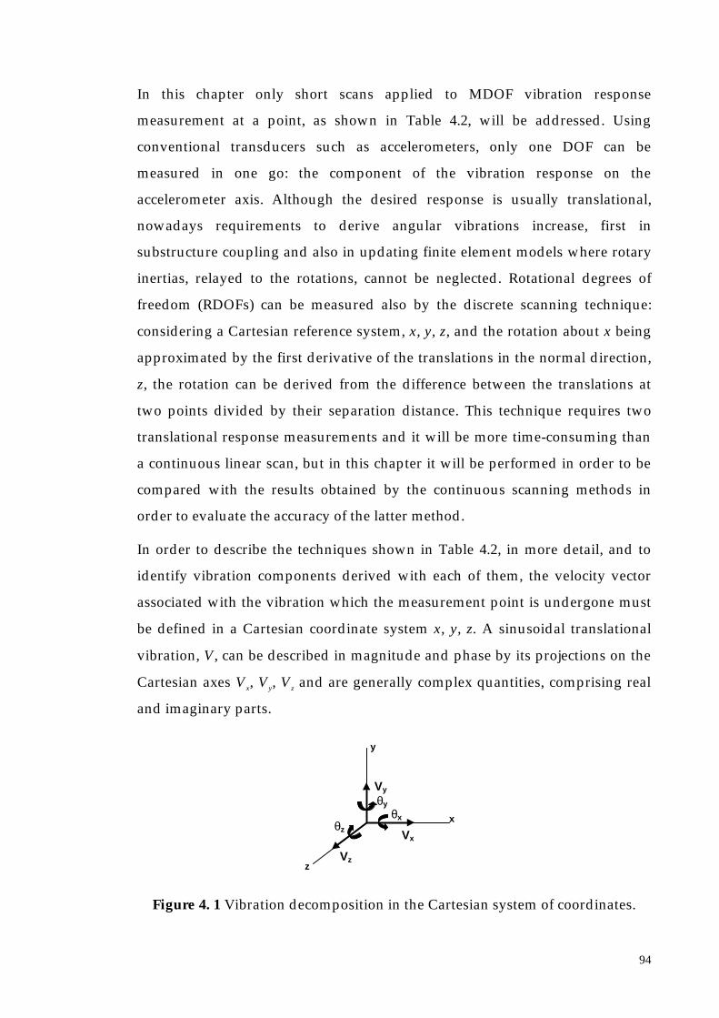
94

In this chapter only short scans applied to MDOF vibration response

measurement at a point, as shown in Table 4.2, will be addressed. Using

conventional transducers such as accelerometers, only one DOF can be

measured in one go: the component of the vibration response on the

accelerometer axis. Although the desired response is usually translational,

nowadays requirements to derive angular vibrations increase, first in

substructure coupling and also in updating finite element models where rotary

inertias, relayed to the rotations, cannot be neglected. Rotational degrees of

freedom (RDOFs) can be measured also by the discrete scanning technique:

considering a Cartesian reference system, x, y, z, and the rotation about x being

approximated by the first derivative of the translations in the normal direction,

z, the rotation can be derived from the difference between the translations at

two points divided by their separation distance. This technique requires two

translational response measurements and it will be more time-consuming than

a continuous linear scan, but in this chapter it will be performed in order to be

compared with the results obtained by the continuous scanning methods in

order to evaluate the accuracy of the latter method.

In order to describe the techniques shown in Table 4.2, in more detail, and to

identify vibration components derived with each of them, the velocity vector

associated with the vibration which the measurement point is undergone must

be defined in a Cartesian coordinate system x, y, z. A sinusoidal translational

vibration, V, can be described in magnitude and phase by its projections on the

Cartesian axes Vx, Vy, Vz and are generally complex quantities, comprising real

and imaginary parts.

Figure 4. 1 Vibration decomposition in the Cartesian system of coordinates.

y

x

z

Vy

Vx

Vz

θyθx

θz

95

Considering an infinitesimal element of structure at the point concerned, three

angular vibration components of the point can be also described. Assuming the

infinitesimal area to behave as a rigid body, i.e. to be a planar, non-deforming

surface, the rotational sinusoidal vibration components on the Cartesian system

θx, θy, θz can be defined (see Figure 4.1).

As shown in Table 4.2, three kinds of short scan can be realised:

- short line scans to recover one translational and one angular vibration,

e.g. Vz and θx , respectively, when the scan lies along the y - direction;

- small circular scans to derive one translational and two angular

vibrations, e.g. Vz and θx and θY respectively if the scanned circle is

contained in x,y plane;

- conical scans, i.e. circular scans on a short-focus lens which focuses the

beam on the point of interest. The laser beam is now moving in a cone

with the vertex in the addressed point, and because its characteristic is to

measure at the direction of its line of sight, the measurement direction is

continuously changing during the rotation. Since three different

directions independent from each other would be enough to derive the

three translational components of the velocity vector, by performing the

conical scan these three DOFs will be recovered in one go. The three

translational vibration components will be Vx, Vy, Vz.

The experimental procedures described above can also be combined together in

order to measure the greatest number of DOFs with the lowest possible number

of measurements. For instance, a conical-circular scan, see Figure 4.2, where the

structure is moved away from the lens focal plane in order to have a circular

path, will be addressed. This technique allows the measurement of 5 DOFs in

only two scans (i.e. the three translational vibration components Vx, Vy, Vz and

two angular vibration about two orthogonal axes lying in the plane of the tested

surface, say θx and θy).

96

Figure 4. 2 Circular-Conical scan.

These techniques suppose that the structure tested undergoes to a sinusoidal

vibration, say, at frequency ω, and it can be assumed to be such that all six DOF

responses are sinusoidal and at the same frequency (though not necessarily in

phase). In this case, describing the laser beam scan frequency as Ω, the LDV

response signal comprises three components: at frequencies ω, (ω + Ω) and

(ω − Ω). Since the Fourier component at (ω − Ω) is necessary for the analysis, it

is important that the LDV scan rate Ω is lower than the vibration frequency, or

else this component appears as a negative frequency, and is not picked up.

Furthermore, a low scan frequency is advantageous, in that it avoids excessive

mechanical loading on the mirror drive system, and minimises mirror-drive

phase shift or delays due to the inertia of the mirrors, an effect which becomes

more important at higher speeds of scanning. Scans in the range 5 Hz to 20 Hz

are generally most satisfactory.

In a continuous scan, the laser spot position is an important datum which needs

to be known. In long scans, whose goal is to recover the ODS along the

trajectory traveled by the beam, only by the identification of the instantaneous

measurement points on the trajectory is it possible to associate the velocity

output to the geometry scanned. In short scans, the position of the

measurement beam at the start of the data acquisition phase allows one to

determine the orientation of the x and y axes on the tested surface and to

identify the velocity vector components completely. This requirement is really

important in circular and conical scans where two angular vibrations or three

translations, respectively, are derived and they need to be distinguished by

relating them to the x and y directions. In the linear scan, it is straightforward to

recover the angular vibration without using any coordinate system convention:

97

the rotation will be simply about the axis perpendicular to the line scan

independently from the definition of x and y. In the circular scan the position of

the laser spot along the circle scanned can be tracked easily by triggering the

acquisition with one of the mirror driver signals. Now, a start position of the

spot in the circle must be defined. At this stage, it is assumed that the mirrors

do not have any inertia and they deflect the laser beam with the same law as the

one they are fed with, i.e. assume that the laser spot will move according to the

sinewaves that drive the mirrors, without any delay, see Figure 4.3. Then the

start point in the circle is point 1 in Figure 4.4 and the direction of the beam is

the one marked in the picture.

0 0.05 0.1 0.15 0.2

-1

-0.5

0

0.5

1

1.5

time (s)

Mirr

or D

river

sig

nal (

V)

x-mirror driver signaly-mirror driver signa

Figure 4. 3 Mirror’s driver signals.

Figure 4. 4 Circular scan configuration.

In order to start the acquisition when the laser spot is in position 1, the LDV

signal acquired must be triggered when the x-axis mirror signal has zero

x

y

point 1

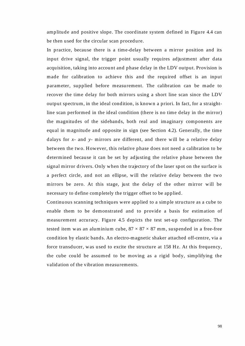
98

amplitude and positive slope. The coordinate system defined in Figure 4.4 can

be then used for the circular scan procedure.

In practice, because there is a time-delay between a mirror position and its

input drive signal, the trigger point usually requires adjustment after data

acquisition, taking into account and phase delay in the LDV output. Provision is

made for calibration to achieve this and the required offset is an input

parameter, supplied before measurement. The calibration can be made to

recover the time delay for both mirrors using a short line scan since the LDV

output spectrum, in the ideal condition, is known a priori. In fact, for a straight-

line scan performed in the ideal condition (there is no time delay in the mirror)

the magnitudes of the sidebands, both real and imaginary components are

equal in magnitude and opposite in sign (see Section 4.2). Generally, the time

dalays for x- and y- mirrors are different, and there will be a relative delay

between the two. However, this relative phase does not need a calibration to be

determined because it can be set by adjusting the relative phase between the

signal mirror drivers. Only when the trajectory of the laser spot on the surface is

a perfect circle, and not an ellipse, will the relative delay between the two

mirrors be zero. At this stage, just the delay of the other mirror will be

necessary to define completely the trigger offset to be applied.

Continuous scanning techniques were applied to a simple structure as a cube to

enable them to be demonstrated and to provide a basis for estimation of

measurement accuracy. Figure 4.5 depicts the test set-up configuration. The

tested item was an aluminium cube, 87 × 87 × 87 mm, suspended in a free-free

condition by elastic bands. An electro-magnetic shaker attached off-centre, via a

force transducer, was used to excite the structure at 158 Hz. At this frequency,

the cube could be assumed to be moving as a rigid body, simplifying the

validation of the vibration measurements.

99

Figure 4. 5 Schematic of the tested structure and the measurement equipment.

The equipment employed consisted of a Polytec Laser Doppler Vibrometer

(optical unit and controller) used as a velocity transducer and made to work as

a CSLDV by driving the scanning system with analogue signals: sinewaves, in

practice. An associated computer hardware and software controlled the scanner

system, driving an arbitrary waveform generator to provide the sinusoidal

excitation and performed the acquisition and the post-process of the measured

data. The output generator/data acquisition and post-processing PC was

provided with:

- a two-channel output card which produced suitable sinewaves to supply

the scanner control driver;

- a GPIB interface to control the sinusoidal force produced via the

arbitrary waveform generator;

- a four-channel input card to acquire the LDV output signal, carrying the

velocity information, the reference signal from the force transducer and

the mirror drive signals to derive the actual position of the laser spot on

the test surface.

In the following sections, the analysis of the LDV signal stored in order to

derive angular and translational vibration at the point of interest is addressed.

If the laser beam scans at frequency, Ω, this frequency will modulate the

forcetransducer

shaker

x

y

z

2 outputcard

4 inputcard

data acquisition andpost process system

mirror signaldriver

LDV output

force reference signal

arbitrarywaveformgenerator

GPIB

100

vibration response of the LDV, giving an output spectrum characteristic for the

occurrence of two sidebands apart from the excitation frequency of ±Ω. From

the response at the sideband frequencies angular deflections can be obtained,

while the translational component is straightforward measured from the

response at the center frequency, i.e. the excitation frequency, ω. Real and

imaginary components of the LDV output spectrum at the mentioned

frequencies, ω, (ω + Ω) and (ω − Ω), are automatically derived from the SLDV

time-record, without passing through a time-consuming FFT process. In fact,

the time history is multiplied by sine and cosine waves at each of these

frequencies in turn, since these frequencies are precisely known a priori. This

procedure has a further advantage which is the small amount of data required

to be stored: rather than record the whole LDV spectrum at each FFT line, only

three (complex) values need to be saved.

4.2. Analysis of Linear Scan and Experimental Validation

Scanning continuously with an LDV beam along a line on a vibrating surface,

the transducer’s output is a modulated signal which indicates the structure’s

vibration. If the mirror driving the beam is fed via a sine wave at frequency Ω,

and assuming the ideal condition where mirror delays can be neglected, the

laser spot will follow a straight line of length 2l over the surface (see Figure 4.6).

Figure 4. 6 Laser beam scan and vibration DOFs associated to the surface.

The position of the spot on the line can be defined at each time instant, t, by:

z

xO

vz

θy

vibratingsurface

LDVbeam

z

xO

2l

A Bstart point

101

tltx Ωcos)( = (4. 1)

A suitable Cartesian coordinate system can be introduced as shown in Figure

4.6: the origin O is at the scan mid-point, the z-direction is the LDV scan-beam

axis and the x- and y-axes are (if set up correctly) parallel to the LDV mirror

deflection axes. The structure vibration at the origin can be derived from the

LDV response, bearing in mind that the line scan must be sufficiently short such

that the structure may be assumed to vibrate as a plane surface. Point O in

Figure 4.6 is then supposed to undergo only to a translational velocity, vz , and

an angular velocity, θy . At a generic point along the line scan the total velocity

can be written as:

( ) yz xvxv θ+= (4. 2)

If a structure’s deflections are sinusoidal at frequency, ω, in general, at any

point:

tttVtVv yIyRyzIzRz ωωθωω sincossincos ΘΘ +=+= (4. 3)

Introducing Equations (4.1) and (4.3) into the Equation (4.2) the structure’s

velocity becomes:

( ) ( )( )tttltVtVtv yIyRzIzR ωωωω sincoscossincos ΘΘΩ +++= (4. 4)

After some manipulation, the response measured by the laser can be shown to

be as:

102

( ) ( )

( ) ( )tltl

tltl

tVtVtv

yRyI

yRyI

zIzR

ΩΘΩΘ

ΩΘΩΘ

+++−

+−−−+

++=

ωω

ωω

ωω

sin2

1cos

2

1

sin2

1cos

2

1

sincos)(

(4. 5)

The LDV output comprises components at the vibration frequency, whose real

and imaginary parts are labelled Rω and Iω, and at a pair of sidebands Rω−Ω and

Iω−Ω and Rω+Ω and Iω+Ω . The sideband components show a characteristic

behaviour: real parts of the left and right sidebands have the same magnitude

but opposite signs, and the same happens for the imaginary components. This

recurrence can be used to calibrate the mirrors, since it is not perfectly realised

when there is a delay of the mirror itself, see Section 4.6. The complex

components of the z-axis translation (VzR and VzI) and x-axis rotations (ΘxR , ΘxI )

may be derived from these Fourier components of the LDV spectrum:

l

R

l

R

l

I

l

I

IVRV

yIyR

zIzR

ΩΩΩΩ ΘΘ −+−+ =−=−==

==

ωωωω

ωω

2222 (4. 6)

Experiments have been carried out in the structure described in Section 4.1 and

illustrated in Figure 4.5. In order to validate the results and to estimate the

reliability of the continuous technique, the conventional discrete procedure has

been performed to measure the translational and angular velocities at point O,

by measuring with the non-scanning LDV at two points A and B (separated by

the same distance as the length of the scan, 2l, see Figure 4.6) using the force

signal as reference. In fact, the rotational DOF can be approximated by the first

derivative of the translations in the normal z-directions, the first derivative

approximation giving:

( ) ( )l

BvAv

y

v zzzy 2

−≈∂∂=θ (4. 7)

103

By measuring the LDV response (translational velocity along the z-axis) in two

steps using the single point LDV working in the conventional way, the RDOF at

the mid point in the conjunction of A and B can be derived. Moreover, the

translational response at O can be obtained as the average of the measurements

at A and B. Two DOFs are then obtained in three shots while the continuous

technique achieves the same result with only one measurement.

In order to compare both amplitude and phase of the two vibration DOFs

measured, it is customary to divide the response by the input forcing to obtain

the FRF, i.e. to refer the vibration to a time datum that is the sinusoidal

excitation. Therefore, forces applied in the continuous scan and in the discrete

point measurement must be acquired at the same time as the corresponding

velocity response.

In the experiments, a drive voltage has been applied to the y-axis laser beam

deflection mirror, so as to scan at 20 Hz along a vertical line 16 mm long,

centred on point O, see Figure 4.7. The translation DOF in the z-direction and

rotation about x were deduced from the ω, (ω + Ω) and (ω − Ω) complex

components using Equations (4.6).

Figure 4. 7 Linear scan set up.

Taking into account the mirror delay that always occurs in reality, by triggering

the acquisition of the LDV signal, this latter appeared to have a modulated time

Oscanline

x

y

z

A

B

excitation

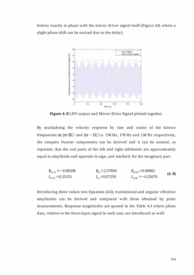
104

history exactly in phase with the mirror driver signal itself (Figure 4.8, where a

slight phase shift can be noticed due to the delay).

0 0.1 0.2 0.3 0.4 0.5

-3

-2

-1

0

1

2

3

4

5

time (s)

Vel

ocity

resp

onse

and

Mirr

or D

river

Sig

nal (

V)

LDV output Mirror Driver signal

Figure 4. 8 LDV output and Mirror Drive Signal plotted together.

By multiplying the velocity response by sine and cosine of the known

frequencies ω, (ω + Ω) and (ω − Ω), i.e. 158 Hz, 178 Hz and 138 Hz respectively,

the complex Fourier components can be derived and it can be noticed, as

expected, that the real parts of the left and right sidebands are approximately

equal in amplitude and opposite in sign, and similarly for the imaginary part.

25670.007259.025353.0

00682.057850.200508.0

−=====−=

+−

+−

ΩΩ

ΩΩ

ωωω

ωωω

III

RRR (4. 8)

Introducing these values into Equation (4.6), translational and angular vibration

amplitudes can be derived and compared with those obtained by point

measurements. Response magnitudes are quoted in the Table 4.3 where phase

data, relative to the force-input signal in each case, are introduced as well:

105

STEADYMEASUREMENT

SCANNINGMEASUREMENT

Translation in z (mag [mm/s]) 12.936 12.911

Translation in z (phase º) -116.89 -117.09

Rotation about x (mag [rad/s]) 0.151 0.159

Rotation about x (phase º) -116.99 -117.26

Table 4. 3 2DOF measurement at point O via linear scan at 20Hz.

The maximum absolute phase discrepancy was 0.27º on the phase of the x-

rotation (around 0.2%). The discrepancy in the measured velocity magnitude

was 0.025 mm/s on the z-translation, inducing again an error of 0.2%. Whereas

the percentage error related to the rotation magnitude was bigger (5.2%) and

this is due to the small amplitude of the angular rotation; in fact, the absolute

discrepancy in the measured rotation magnitude was 0.008 rad/s.

4.3. Analysis of Circular Scan and Experimental Validation

If the laser beam is scanned continuously at a speed, Ω, in a circle of radius, R,

centred on the nominal measurement point, the vibration response measured at

an arbitrary position on the circle, say, Q, of general coordinates x,y will be:

xyvyxv yxz θθ ++=),( (4. 9)

Positive directions of rotations θx and θy are shown in Figure 4.9.

106

Figure 4. 9 Circular scan configuration.

The laser spot is moving around the circle at speed, Ω, and so the angle swept

when it is passing through Q will be Ωt. The coordinates of the point Q

expressed in terms of scan speed are:

( )( )tRy

tRx

ΩΩ

cos

sin

==

(4. 10)

R being the circle radius. Equation (4.9) will then become:

tRtRvtv yxz ΩΩ sincos)( θθ ++= (4. 11)

If the surface vibration is harmonic, at frequency ω, the translational and

rotational components can be expressed as:

tttt

tVtVv

yIyRyxIxRx

zIzRz

ωωθωωθωω

sincossincos

sincos

ΘΘΘΘ +=+=+=

(4. 12)

So, Equation (4.11) can be rewritten as:

vz

rotx

roty

θx

θy

Q

Q’

x

y

z

RΩt

Q

x

y

H

K

rot x = θx × distance(Q’-x axis) = θx × QK = θx × y

rot y = θy × distance(Q’-y axis) = θy × QH = θy × x

startpoint

107

ttRttR

ttRttR

tVtVtv

yIyR

xIxR

zIzR

ΩΘΩΘΩΘΩΘ

sinsinsincos

cossincoscos

sincos)(

ωωωω

ωω

+++++

++=(4. 13)

Expanding:

tRtR

tRtR

tVtVtv

yRxIyIxR

yRxIyIxR

zIzR

)sin()(2

1)cos()(

2

1

)sin()(2

1)cos()(

2

1

sincos)(

ΩΘΘΩΘΘ

ΩΘΘΩΘΘ

++++−+

+−−+−++

++=

ωω

ωω

ωω

(4. 14)

whence,

−=

−=

+=

+=

==

+−−+

+−+−

R

RR

R

II

R

II

R

RR

IVRV

yIyR

xIxR

zIzR

ΩΩΩΩ

ΩΩΩΩ

ΘΘ

ΘΘ

ωωωω

ωωωω

ωω

(4. 15)

The real and imaginary components of the z-axis translation (VzR and VzI) and

the x- and y-axis rotations (ΘxR , ΘxI , ΘyR , ΘyI ) are easily derived from the real and

imaginary components of the LDV response using Equations (4.15) (the z-axis

being the central axis around which the laser scan rotates).

Measurements have been again made on the cube test piece to validate the

analysis of small-radius circular scanning. The same set up shown in Figure 4.5

has been used here. Drive voltages have been applied to the x- and y- laser

beam deflection mirrors, so as to scan the beam at 20 Hz around a circle of 16

mm diameter, centred on point O, see Figure 4.10.

108

Figure 4. 10 Circular scan set up.

The translation DOF, Vz , and the rotational DOFs Θx and Θy , were derived

using Equation (4.15) from the real and imaginary components of the LDV

output spectrum recovered by multiplying the time acquired history by sines

and cosines at the usual frequencies (138 Hz, 158 Hz and 178 Hz). The same

procedure followed in Section 4.2 to validate the continuous technique has been

applied here as well, i.e. via a non-scanning LDV, and translational vibration at

four points A, B, C, E (Figure 4.10) were measured using the force signal as

reference. The distances A-B and C-E were the same as the circle-scan diameter.

Translation and rotation DOF derivation using measurements from four points

is based on the same procedure as for two points (Section 4.2).

Steady measurements are compared with the results from the circular scan in

the Table 4.4 (phase data are again relative to the corresponding force input

signal stored in each case).

O

scancircle

x

y

z

A

excitation

B

E

C

109

STEADYMEASUREMENT

SCANNINGMEASUREMENT

Translation in z (mag [mm/s]) 12.970 13.101

Translation in z (phase º) -116.97 -117.05

Rotation about x (mag [rad/s]) 0.043 0.061

Rotation about x (phase º) 67.91 68.35

Rotation about y (mag [rad/s]) 0.290 0.299

Rotation about y (phase º) 62.87 64.32

Table 4. 4 MDOF measurement at point O via circular scan at 20Hz.

In these measurements, the difference in the measured translation velocity

magnitude was 0.131 mm/s ( 1.01 %), the maximum phase discrepancy was

1.45º (rotation about y). The worst rotation magnitude discrepancy was 0.018

rad/s (6.2%). Rotation measurement uncertainty obviously depends on the scan

radius; in this case 0.018 rad/s uncertainty in Θx corresponds to a translational

uncertainty of 0.14mm/s, 1.11% of the overall signal amplitude.

4.4. Analysis of Conical Scan and Experimental Validation

The three translational degrees of freedom at a point in a vibrating structure, Vx

Vy Vz, can be measured by a tri-axial accelerometer but the same result can be

achieved by using an LDV with the advantage of overtaking the well-known

mass-loading effect. The translational velocity components may be recovered

by performing three separate non-contact measurements at different directions

(each mutually independent, i.e. not belonging at the same plane) via a

conventional single-axis laser vibrometer focused to the same measurement

point. Moreover, an LDV can be directed at the target point while the laser

beam exercises a conical scan; the philosophy is the same as the three

directional measurements procedure but the three directions are now swept

with one shot.

In practice, the laser beam is scanned in a circle, at frequency Ω, the circular

scan being diverted by an annular mirror or a short-focus lens so that the focal

110

point is scanned in a circular cone with an angle of incidence Φ, as shown in

Figure 4.11.

Figure 4. 11 Conical scan configuration.

With the scan arranged as in Figure 4.11, specifically see detail (b), the vibration

signal detected at an arbitrary angular position, ϕ, along the scan cone is

ΦΦΦ sin)(cos)(sin)(sin)(cos)()( ttvttvtvtv yxz ϕϕϕ ++= (4. 16)

where, Φ, is the lens deviation angle (cone angle) and, ϕ, is the scanned angle or

Ωt, Ω being the scan speed. The mirrors are driven following again Equation

(4.10) with a suitable radius, R, in order to make the laser beam scan in a circle

inside the lens.

Considering the surface to be vibrating sinusoidally at frequency, ω, the three

translational components can be written as:

tVtVv

tVtVv

tVtVv

zIzRz

yIyRy

xIxRx

ωωωωωω

sincos

sincos

sincos

+=

+=+=

(4. 17)

ϕstartpoint

Q

vx

vy

x

y

vx sinϕ

vy cosϕ

(b) x-y plane projection

z

vz

vy cosϕ

vx sinϕ

vx sinϕ

vy cosϕ sinΦ

vz cosΦ

Q

Φ

(c) Q-z plane projection

(a) 2-D view

x

y

z

startpoint

ϕ

Φ

V

vx

vz

vy

Q-z plane

Q

111

Introducing the previous expressions in Equation (4.16), the vibration velocity

will appear as:

( ) ( )( ) ΦΩ

ΦΩΦsincossincos

sinsinsincoscossincos)(

ttVtV

ttVtVtVtVtv

yIyR

xIxRzIzR

ωωωωωω

+++++=

(4. 18)

Expanding:

tVVtVV

tVVrtVV

tVtVtv

yIxRxIyR

xRyIyRxI

zIzR

)sin(sin)(2

1)cos(sin)(

2

1

)sin(sin)(2

1)cos(sin)(

2

1

sincoscoscos)(

ΩΦΩΦ

ΩΦΩΦ

ΦΦ

++++−+

+−−+−++

++=

ωω

ωω

ωω

(4. 19)

The LDV output has a single sideband-pair spectrum and, using the same

notation as before, the real and imaginary components of the velocities in the

Cartesian system of reference may be derived:

ΦΦ

ΦΦ

ΦΦΩΩΩΩ

ΩΩΩΩ

coscos

sinsin

sinsin

ωω

ωωωω

ωωωω

IV

RV

IIV

RRV

RRV

IIV

zIzR

yIyR

xIxR

==

+=+=

−=−=

−++−

+−−+

(4. 20)

Translational velocity has been measured at a point O on the cube: the free-free

cube excited at the natural frequency of 158 Hz. The laser beam was scanned

continuously in a conical path directed at the target point, see Figure 4.12.

112

Figure 4. 12 Conical scan set up.

The conical scan was realised by employing a single-element 67 mm diameter,

plano-convex condenser lens with a focal length of about 45 mm. The maximum

scan angle, Φ, that could be achieved with this lens was 36.66°, when the scan

was performed at the lens edge as shown in Figure 4.13.

Figure 4. 13 Lens deviation angle.

The cone angle can be determined precisely by calibration, see Section 4.6, but it

was found that this angle was always fluctuating around 30º if the scan circle on

the lens was set at about 2 mm from its circumferential edge.

The laser beam was driven to follow a circular path by feeding the x- and y-

mirrors via two sinewaves 90º phase shifted described by Equations (4.10),

67 m

m

45 mm

fΦ

O

scancone

x

y

z

excitation

lens

113

where R is the scan circle radius (about 31.5 mm) and Ω is the scan speed that

was chosen to be 10 Hz.

The focusing process was easily carried out, in fact, since the laser beam is

constituted of coherent monochromatic light, and if it is made to scan around a

circle centred on the lens’s optical axis, no aberration fluctuations are produced.

The standoff distance was adjusted until, when scanning, the circle produced

on the illuminated surface degenerated to a point.

Curve fitting the modulated LDV output signal at 158 Hz and 158 ± 10 Hz real

and imaginary components at the excitation and sideband frequencies are

recovered (Rω , Iω , and Rω−Ω , Iω−Ω , Rω+Ω , Iω+Ω ). By applying Equation 4.20,

translational DOFs can be established in amplitude and phase relative to the

force input signal. Their values are reported in Table 4.5.

Amplitude (mm/s) Phase (º)

Translation in x 9.720 -124.03

Translation in y 0.926 56.16

Translation in z 6.517 -119.02

Table 4. 5 MDOF measurement at point O via conical scan at 10Hz.

An alternative analysis of the conical scanning technique in cylindrical

coordinates, see reference [9], may be helpful to facilitate the processing of the

data acquired. It is possible to derive the velocity magnitude, V, and its vector

orientation angles, γ and δ, knowing magnitude and phase values of the central

peak and sidebands in the velocity spectrum. In order to do this it is necessary

to transform the formulae previously derived in cylindrical coordinates into

Cartesian coordinates. The vibration vector, v, expressed by the coordinates (vx ,

vy , vz) in the Cartesian reference system, will be now identified by the

cylindrical co-ordinates (V, δ, γ ). A relationship between rectangular and

cylindrical coordinates can be easily established by geometrical considerations,

see Figure 4.14. Note that this visualisation can be made only if the vibration

velocity vector lies on a straight line in the x,y plane, i.e. if the x- and y-

components of the vibration response are in- or out-of-phase with each other.

114

Figure 4. 14 Cylindrical representation of vibration vector.

The velocity Cartesian components can be written in terms of the cylindrical

coordinates:

δγδγ

γ

sinsin

cossin

cos

Vv

Vv

Vv

y

x

z

===

(4. 21)

Because the amplitude vibration is harmonic, it can be represented as:

tVtVV IR ωω sincos += (4. 22)

Introducing Equation (4.22) into (4.21), and in Equation (4.16), the full

expression for the velocity at time t can be derived:

( )( )( ) Φ

ΦΦ

sin)(cossinsinsincos

sin)(sincossinsincos

coscossincos)(

ttVtV

ttVtV

tVtVtv

IR

IR

IR

ϕδγωωϕδγωω

γωωθ

+++++

++= (4. 23)

(a) 2-D view

x

y

z

V

vx

vz

vy

V-z planeV sinγ

δ

(d) x-y plane projection

vx

vy

x

y

V sinγ

δ

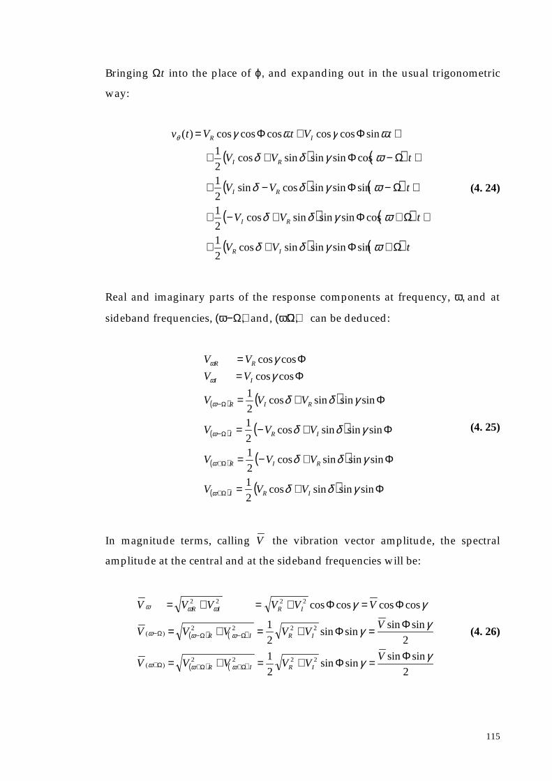
115

Bringing Ωt into the place of ϕ, and expanding out in the usual trigonometric

way:

( ) ( )

( ) ( )

( ) ( )

( ) ( )tVV

tVV

tVV

tVV

tVtVtv

IR

RI

RI

RI

IR

ΩΦ

ΩΦ

ΩΦ

ΩΦ

ΦΦ

+++

+++−+

+−−+

+−++

++=

ωγδδ

ωγδδ

ωγδδ

ωγδδ

ωγωγθ

sinsinsinsincos21

cossinsinsincos21

sinsinsincossin2

1

cossinsinsincos21

sincoscoscoscoscos)(

(4. 24)

Real and imaginary parts of the response components at frequency, ω, and at

sideband frequencies, (ω−Ω), and, (ω+Ω), can be deduced:

( ) ( )

( ) ( )

( ) ( )

( ) ( ) Φ

Φ

Φ

Φ

ΦΦ

Ω

Ω

Ω

Ω

sinsinsincos2

1

sinsinsincos2

1

sinsinsincos2

1

sinsinsincos2

1

coscos

coscos

γδδ

γδδ

γδδ

γδδ

γγ

ω

ω

ω

ω

ω

ω

IRI

RIR

IRI

RIR

II

RR

VVV

VVV

VVV

VVV

VV

VV

+=

+−=

+−=

+=

==

+

+

−

−

(4. 25)

In magnitude terms, calling V the vibration vector amplitude, the spectral

amplitude at the central and at the sideband frequencies will be:

( ) ( )

( ) ( ) 2

sinsinsinsin

2

1

2

sinsinsinsin

2

1

coscoscoscos

2222)(

2222)(

2222

γγ

γγ

γγ

ωωω

ωωω

ωωω

ΦΦ

ΦΦ

ΦΦ

ΩΩΩ

ΩΩΩ

VVVVVV

VVVVVV

VVVVVV

IRIR

IRIR

IRIR

=+=+=

=+=+=

=+=+=

+++

−−− (4. 26)

116

V and γ may be derived from the previous equations considering the following

relationships:

γ

γ

ωω

ω

sinsin

coscos

)()(V

VV

VV

=+

=

+−

Φ

ΦΩΩ

(4. 27)

By squaring and summing the previous two equations, the velocity vector

magnitude is deduced:

( ) ( )22

sincos

++

= +−

ΦΦΩΩ ωωω VVV

V (4. 28)

Using Equations (4.27), the angular position with respect the z-direction can be

established as well, by:

+= +−−

ΦΩΩ

tan

1tan )()(

ω

ωωγV

VV1 (4. 29)

Angle δ may be derived from the measured phase data at the sideband

frequencies. The calculation is made easier if the sinusoidal vibration -depicted

in Equation (4.22)- is written in terms of amplitude and phase instead of real

and imaginary components:

)cos( αω += tVV (4. 30)

α, being the response phase angle relative to a reference that is usually the

applied forcing input.

In order to make Equations (4.30) and (4.22) coincide, real and imaginary

components must be expressed in terms of magnitude and phase of the

vibration vector:

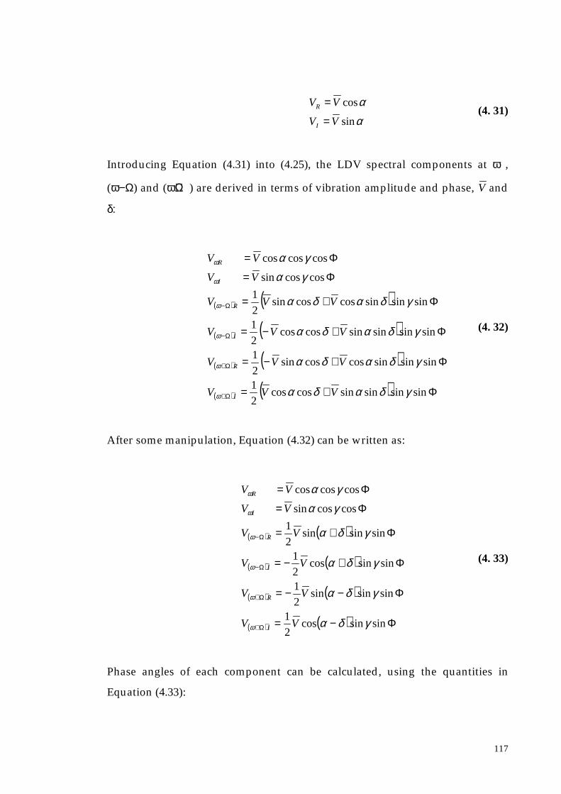
117

αα

sin

cos

VV

VV

I

R

=

=(4. 31)

Introducing Equation (4.31) into (4.25), the LDV spectral components at ω ,

(ω−Ω) and (ω+Ω) are derived in terms of vibration amplitude and phase, V and

δ:

( ) ( )

( ) ( )

( ) ( )

( ) ( ) Φ

Φ

Φ

Φ

Φ

Φ

Ω

Ω

Ω

Ω

sinsinsinsincoscos2

1

sinsinsincoscossin2

1

sinsinsinsincoscos2

1

sinsinsincoscossin2

1

coscossin

coscoscos

γδαδα

γδαδα

γδαδα

γδαδα

γαγα

ω

ω

ω

ω

ω

ω

VVV

VVV

VVV

VVV

VV

VV

I

R

I

R

I

R

+=

+−=

+−=

+=

=

=

+

+

−

−

(4. 32)

After some manipulation, Equation (4.32) can be written as:

( ) ( )

( ) ( )

( ) ( )

( ) ( ) Φ

Φ

Φ

Φ

Φ

Φ

Ω

Ω

Ω

Ω

sinsincos2

1

sinsinsin21

sinsincos2

1

sinsinsin2

1

coscossin

coscoscos

γδα

γδα

γδα

γδα

γαγα

ω

ω

ω

ω

ω

ω

−=

−−=

+−=

+=

=

=

+

+

−

−

VV

VV

VV

VV

VV

VV

I

R

I

R

I

R

(4. 33)

Phase angles of each component can be calculated, using the quantities in

Equation (4.33):

118

( )( )

( )

( )( )

( )

( )

( )( )

( )

( )( )

( )

( ) 22

cos

2sin

tansin

costantan

22

cos

2sin

tansin

costantan

cos

sintantantan

111

111

111

πδαδαπ

δαπ

δαδα

πδαδαπ

δαπ

δαδα

ααα

ω

ωω

ω

ωω

ω

ωω

−−=

−−

−−

−=

−−−=

=∠

−+=

+−

+−

−=

++−=

=∠

=

=

=

=∠

−−

+

+−+

−−

−

−−−

−−−

R

I

R

I

R

I

R

I

V

VV

V

VV

V

V

V

V

V

VV

Ω

ΩΩ

Ω

ΩΩ

(4. 34)

It can be noticed that the phase at the excitation frequency corresponds directly

to the vibration phase while the third angular coordinate of the vibration vector

is established from the difference of the phases at the sideband frequencies:

( ) ( )

2ΩΩ +− ∠−∠

= ωωδVV

(4. 35)

From Equations (4.28), (4.29) and (4.35) the three cylindrical components of the

vibration vector (V , γ, δ) can thus be obtained.

The accuracy of the method has been checked by comparing the conical

scanning results with corresponding velocities measured by a single-axis

accelerometer directly mounted on the vibrating platform of a shaker, see

Figure 4.15. With this set-up the velocity of the top surface of the accelerometer

was expected to be in a direction perpendicular to its surface. The point O,

shown in Figure 4.12, was, in this case, the centre point of the accelerometer’s

top surface.

119

Figure 4. 15 Accelerometer/Shaker set-up for Conical Scan trial.

Vibration velocities were measured simultaneously using both the

accelerometer and the conical-scanning LDV, changing the angle of incidence of

the laser beam axis to the surface of the accelerometer (γ) in order to visualise

the measurement accuracy at different direction of acquisition. For conical

scanning, the LDV beam was made to follow a circular trajectory by supplying

sine and cosine signals at 20 Hz to the mirror drive inputs, the voltages being

adjusted to scan in a circle near the periphery of the lens.

From Equation (4.20), vibration magnitudes Vx , Vy , Vz , in the x-, y-, z-directions

can be obtained combining real and imaginary components. The velocity vector

modulus V is:

222zyx VVVV ++= (4. 36)

This value was compared with the velocity magnitude derived from the

accelerometer with the results shown in Table 4.6. In Figure 4.16 the velocity

outputs of the LDV and of the accelerometer, listed in the second and third

columns of Table 4.6 respectively, are plotted against the incidence angle, γ.

(a) 2D view

x

y

z

lens

O

accelerometer

shaker

(b) Top view

Θ

V

accelerometer

γ

120

ANGLE(º)

From LDV OUTPUT(mm/s)

From ACCELEROMETER OUTPUT(mm/s)

DISCREPANCY(%)

0 29.049 28.404 2.278

5 30.215 28.562 5.784

10 30.507 28.615 6.612

15 30.753 28.545 7.735

20 27.924 27.473 1.641

25 28.309 26.224 7.951

30 27.578 26.223 5.163

35 28.828 28.443 1.353

40 29.008 28.615 1.373

45 29.094 28.478 2.163

50 27.88 28.439 1.965

Table 4. 6 Vibration velocity amplitudes measured with a conical scan LDV and

an accelerometer.

Figure 4. 16 Vibration velocity amplitude measured with a conical scan

LDV and an accelerometer.

With this test set-up, it was found that the vibration vector was not exactly in

the direction of the accelerometer’s axis. In fact, there were sidebands to the

LDV response even if the scan axis was perpendicular to the accelerometer’s top

surface. This means that the LDV was observing also sideways velocities Vx and

Vy. The reason was found to be because the motion of the shaker platform was

not exactly perpendicular to its mounting plane. The deviation varied with

excitation frequency, being as low as 2° at 400Hz. Therefore discrepancies

0 10 20 30 40 500

5

10

15

20

25

30

35

40

45

50

Vib

ratio

n ve

loci

ty (m

m/s

)

Incidence angle (deg)

LASERACCELEROMETER

121

between the two measurements appeared to be rather significant (up to around

8%).

In order to improve the accuracy test, a second check was performed with a

different test specimen and with the purpose in investigating the accuracy of

the angle (γ) measured. The alternative way of recovering the vibration vector

in cylindrical coordinates was used in this case, see Equation (4.29).

Tests were conducted using an aluminium cantilever beam, 25 mm wide, 6.5

mm thick and 180 mm long, clamped at one end to a heavy block to produce,

essentially, a simple cantilever, Figure 4.17. When excited at its lowest natural

frequency, 84.5Hz, the motion was expected to be perpendicular to the face of

the beam.

Figure 4. 17 Conical scan set-up on the beam.

The cantilever beam was inclined to the conical scan axis in a series of different

set-ups with angles of incidence between 0º and 55º in steps of 5º and at each

step the (corresponding) angle γ was calculated using Equation (4.29). The

results are listed in Table 4.7.

(a) 2D view

zlens

cantileverbeam

shaker

y

xO

Θ

V

cantileverbeam

γ

(b) Top view

122

TRUE ANGLE γ (º) MEASURED ANGLE γ (º) ERROR (º)

0 2.11 2.11

5 4.951 0.049

10 8.394 1.606

15 15.039 0.039

20 18.599 1.401

25 24.827 0.173

30 31.022 1.022

35 34.642 0.358

40 41.569 1.569

45 46.688 1.688

50 52.466 2.466

55 58.238 3.238

Table 4. 7 Measured angles using conical scan.

Measured values are plotted against the true ones in the following graph

(Figure 4.18):

Figure 4. 18 Accuracy of Vibration Direction measured by Conical Scan.

The worst discrepancies were obtained at the smallest and the largest angles.

Uncertainties associated with the measurements at high incidence angles may

be associated with an apparent increase in speckle noise in the LDV output. It is

clearly impossible to apply a conical scan at angles of incidence to a surface

greater than the cone scan angle. At high angles of incidence, the light returned

to the laser unit was reduced and the LDV signal was heavily polluted with

0 10 20 30 40 50 600

10

20

30

40

50

60

Incidence angle (deg)

Vib

ratio

n an

gle

(deg

)

MEASUREDTRUE

123

signal dropouts. The speckle noise was generally low below a nominal

incidence of 40º but increased above this (Figure 4.19), as the scan angle on one

side approached grazing incidence. There was also considerable difficulty in

focusing the laser spot on the test surface when its inclination to the cone axis

was high. Measurement accuracy was optimized by using retro-reflective tape

attached at the test point on the structure.

Figure 4. 19 Noise floor outline.

At small angles of inclination, the sidebands, which represent the test surface

rotation angle, are relatively small and the analysis error becomes larger, as the

sidebands become confused with the noise.

An accuracy analysis can be applied to the angle derived if the uncertainty of

the peak amplitudes in the LDV output spectrum is known. Ten measurements

of the central peak and sideband amplitudes were acquired using the set-up

shown in Figure 4.17, with an inclination angle of 10º. The errors relative to the

main value of each parameter have been calculated as a standard deviation and

are reported in Table 4.8:

0 10 20 30 40 50 600

0.02

0.04

0.06

0.08

0.1

0.12

0.14

0.16

0.18

Incidence angle(deg)

Flo

or n

oise

(V)

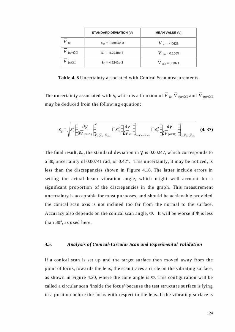
124

STANDARD DEVIATION (V) MEAN VALUE (V)

V ω εω = 3.8887e-3 V m = 4.0623

V (ω−Ω) ε- = 4.2239e-3 V m- = 0.1065

V (ω+Ω) ε+ = 4.2241e-3 V m+ = 0.1071

Table 4. 8 Uncertainty associated with Conical Scan measurements.

The uncertainty associated with γ, which is a function of V ω, V (ω−Ω), and V (ω−Ω),

may be deduced from the following equation:

2

,,)(

22

,,

2

2

,,)(

2

+−+−+−

∂

∂+

∂∂+

∂

∂=+

+−

−mmmmmmmmm VVVVVVVVV VVV ΩΩ ωω

ωω

γγεγεγεε (4. 37)

The final result, εγ , the standard deviation in γ, is 0.00247, which corresponds to

a 3εγ uncertainty of 0.00741 rad, or 0.42°. This uncertainty, it may be noticed, is

less than the discrepancies shown in Figure 4.18. The latter include errors in

setting the actual beam vibration angle, which might well account for a

significant proportion of the discrepancies in the graph. This measurement

uncertainty is acceptable for most purposes, and should be achievable provided

the conical scan axis is not inclined too far from the normal to the surface.

Accuracy also depends on the conical scan angle, Φ. It will be worse if Φ is less

than 30°, as used here.

4.5. Analysis of Conical-Circular Scan and Experimental Validation

If a conical scan is set up and the target surface then moved away from the

point of focus, towards the lens, the scan traces a circle on the vibrating surface,

as shown in Figure 4.20, where the cone angle is Φ. This configuration will be

called a circular scan ‘inside the focus’ because the test structure surface is lying

in a position before the focus with respect to the lens. If the vibrating surface is

125

moved away from the lens, a circular scan ‘outside the focus’ will be realised; in

fact, the test structure surface is now positioned beyond the focal plane of the

lens. If the distance between the focus and the structure surface in both the

configurations is the same (d), the circle scanned by the laser will be similar

(same radius R) but the start point in the circle will undergo to a shift of 180º. In

Figure 4.20 it can be noticed that the start point in the inside-focus configuration

is situated in the first quadrant while in the outside-focus configuration it is in

the third one.

Figure 4. 20 Conical-circular scan configuration.

Two measurements of this type enable z-axis translation and x-axis and y-axis

translation and rotation DOFs to be resolved.

For the inside-focus configuration, at time instant t, the laser spot will coincide

with the point QIN defined by its at angular position, ϕ(t). If the scan speed is Ω,

the angle ϕ is expressed by Ωt. At point QIN, the laser beam, whose

measurement direction is dictated by the cone angle Φ, will be then sensitive

to the three translational DOFs (vx, vy, vz) and the two rotation DOFs (θx , θy),

x

y

z

startpoint

QIN

ϕΦ

startpointIN

lensfocus

x

yz

startpointOUT

QOUT

ϕ Test surfaceoutside the focus

Test surfaceinside the focus

d

d

R

R

126

which are, in a vectorial representation, θxRcosϕ and θyRsinϕ: see Figure 4.9 in

Section 4.3. The velocity measured at point QIN will be:

ΦΦ

ΦΦΦ

cos)(sin)(cos)(cos)(

sin)(cos)(sin)(sin)(cos)()(

tRttRt

ttvttvtvtv

yx

yxzIN

ϕθϕθϕϕϕ

++

+++=(4. 38)

The complete vibration signal, given in the previous equation, can be deduced

geometrically as shown in Figure 4.21.

Figure 4. 21 Inside-focus conical-circular scan.

(a) 2-D view

x

z

y

startpoint

QIN

ϕΦ

V

vx

vz

vy

QIN-z plane

startpointIN θx

θy

R


x

ystartpointIN

QIN

ϕ

vx

vy

vx sinϕ

vy cosϕ

R

(c) QIN-z plane projection

vz

vy cosϕ

vx sinϕ

vx sinϕ sinΦ

vy cosϕ sinΦ

vz cosΦ

z

QIN

Φ

scan circle

θx Rcosϕ

θy Rsinϕ

θyRsinϕ cosΦ

θxRcosϕ cosΦ

127

Considering the test structure to be undergoing a complex sinusoidal motion,

the vibration DOFs, in terms of their real and imaginary components, can be

expressed as:

tVtVtv

ttttVtVtv

ttttVtVtv

zIzRz

yIyRyyIyRy

xIxRxxIxRx

ωωωωθωωωωθωω

sincos)(

sincos)(sincos)(

sincos)(sincos)(

+=

+=+=+=+=

ΘΘΘΘ

(4.39)

These quantities can be substituted into the vibration velocity expression given

by Equation (4.38) and the following relationship developed:

ttRttR

ttRttR

ttVttV

ttVttV

tVtVtv

yIyR

xIxR

yIyR

xIxR

zIzRIN

ΩΦΘΩΦΘΩΦΘΩΦΘ

ΩΦΩΦΩΦΩΦ

ΦΦ

sinsincossincoscos

cossincoscoscoscos

cossinsincoscossin

sinsinsinsincossin

sincoscoscos)(

ωωωω

ωωωω

ωω

+++++

++++++

++=

(4. 40)

where the quantity Ωt takes the place of the scanned angle, ϕ. Expanding out,

we obtain:

( ) ( ) ( )

( ) ( ) ( )

( ) ( ) ( )

( ) ( ) ( )tRVV

tR

VV

tR

VV

tR

VV

tVtVtv

yRxIxRyI

yIxRxIyR

yRxIxRyI

yIxRxIyR

zIzRIN

ΩΦΘΘΦ

ΩΦΘΘΦ

ΩΦΘΘΦ

ΩΦΘΘΦ

ΦΦ

+

++++

++

−+−+

+−

−+−+

+−

++++

++=

ω

ω

ω

ω

ωω

sincos2

sin2

1

coscos2

sin2

1

sincos2

sin2

1

coscos2

sin2

1

sincoscoscos)(

(4. 41)

128

The real (cosine term) and imaginary (sine term) parts of the components at the

centre and sideband LDV output frequencies are thus:

( ) ( ) ( )

( ) ( ) ( )

( ) ( ) ( )

( ) ( ) ( ) ΦΘΘΦ

ΦΘΘΦ

ΦΘΘΦ

ΦΘΘΦ

ΦΦ

Ω

Ω

Ω

Ω

cos2

sin2

1

cos2

sin2

1

cos2

sin2

1

cos2

sin2

1

coscos

yRxIxRyIIN

yIxRxIyRIN

yRxIxRyIIN

yIxRxIyRIN

zIINzRIN

RVVI

RVVR

RVVI

RVVR

VIVR

+++=

−+−=

−+−=

+++=

==

+

+

−

−

ω

ω

ω

ω

ωω

(4. 42)

In this system of equations there are eight unknowns (VxR , VxI , VyR , VyI , ΘxR , ΘxI

ΘyR, ΘyI) but only four equations. However by using ones derived for the second

conical-circular scan configuration (outside-focus configuration), a further four

equations are developed and the system can be solved. This situation is

described in Figure 4.22, where it is possible to note that at point QOUT the

sensitivity to vx, vy, and vz, are unchanged, but the responses to θx , and θy are

phase-reversed because the scanned point is at the opposite end of a diameter

of the scan circle.

Equation (4.38) therefore becomes:

ΦΦ

ΦΦΦ

cos)(sin)(cos)(cos)(

sin)(cos)(sin)(sin)(cos)()(

tRttRt

ttvttvtvtv

yx

yxzOUT

ϕθϕθϕϕϕ

−−

+++=(4. 43)

The LDV response components are hence given by a small modification of

Equations (4.42):

129

( ) ( ) ( )

( ) ( ) ( )

( ) ( ) ( )

( ) ( ) ( ) ΦΘΘΦ

ΦΘΘΦ

ΦΘΘΦ

ΦΘΘΦ

ΦΦ

Ω

Ω

Ω

Ω

cos2

sin2

1

cos2

sin2

1

cos2

sin2

1

cos2

sin2

1

coscos

yRxIxRyIOUT

yIxRxIyROUT

yRxIxRyIOUT

yIxRxIyROUT

zIOUTzROUT

RVVI

RVVR

RVVI

RVVR

VIVR

+−+=

−−−=

−−−=

+−+=

==

+

+

−

−

ω

ω

ω

ω

ωω

(4. 44)

Figure 4. 22 Outside-focus conical-circular scan.

(a) 2-D view

z

x

y

startpoint

QIN

ϕ

Φ

V

vx

vz

vy

QIN-z planestartpointIN

θx

θy

R


x

QOUT

y

startpointOUT

ϕ

vx

vy

vx sinϕ

vy cosϕ

R

(c) QIN-z plane projection

vz

vy cosϕ

vx sinϕ

vx sinϕ sinΦ

vy cosϕ sinΦ

vz cosΦ

z

QOUT

Φ

scan circle

θx Rcosϕ

θy Rsinϕ

θyRsinϕ cosΦ

θxRcosϕ cosΦ

130

Combining Equations (4.42) and (4.44) together, there is sufficient information

to extract the required five DOF vibration components, the unknowns Vx ,

Vy , Vz , Θx , and Θy.

ΦΘ

ΦΘ

ΦΘ

ΦΘ

ΦΦ

ΦΦ

ΦΦΦΦ

ΩΩΩΩΩΩΩΩ

ΩΩΩΩΩΩΩΩ

ΩΩΩΩΩΩΩΩ

ΩΩΩΩΩΩΩΩ

cos2cos2

cos2cos2

sin2sin2

sin2sin2

coscoscoscos

)()()()()()()()(

)()()()()()()()(

)()()()()()()()(

)()()()()()()()(

R

RRRR

R

IIIIR

IIII

R

RRRR

IIIIV

RRRRV

RRRRV

IIIIV

IIV

RRV

OUTOUTININyI

OUTOUTININyR

OUTOUTININxI

OUTOUTININxR

OUTOUTININyI

OUTOUTININyR

OUTOUTININxI

OUTOUTININxR

OUTINzI

OUTINzR

+−+−−+−+

−+−+−+−+

−+−+−+−+

−++−−+−+

+−−=

+−−=

−−+=

−−+=

+++=

+++=

+−−=

−+−=

====

ωωωωωωωω

ωωωωωωωω

ωωωωωωωω

ωωωωωωωω

ωωωω

(4. 45)

It is worth emphasising that circular and conical scans are special cases of the

conical-circular scan theory, and this section therefore serves as a derivation for

Equations (4.15) and (4.20) respectively.

If the cone angle, Φ, approaches zero, the test set up becomes equivalent to a

circular scan situation and Equations (4.45) will take the form of Equations

(4.15). The circular scan can thus be seen as a particular conical-circular scan

where the lens has a focal plane at infinite distance (see Figure 4.23). This

produces the effect of moving the outside-focus configuration to infinity as well

and then of preventing its use in the process.

Figure 4. 23 Conical-circular scan degeneration for Φ going to zero.

f

Φ

f ➀ f → ∞

INSIDE-FOCUS

OUTSIDE-FOCUS ➀

OUTSIDE-FOCUS

Φ → 0

OUTSIDE-FOCUS

→ ∞

131

Only Equation (4.41) will then be available but it will be sufficient to solve the

remaining DOFs VzR, VzI, ΘxR, ΘxI, ΘyR, ΘyI , since the other ones -VxR , VxI , VyR , VyI-

disappeared, being multiplied by sinΦ, which is zero. Therefore, Equation (4.41)

will become the same as Equation (4.14), representing the vibration velocity in

the case of a circular scan, and from it the relevant DOF components can be

derived.

Similarly, if the scan radius becomes zero, that leads to a conical scan, the two

circles degenerating to a point coincident with the lens focus, and Equations

(4.45) simplify to those of Equations (4.20) in Section 4.4. In fact, components in

the outside-focus configuration will assume the same values of the ones in the

inside-focus configuration: ( ) ( ) ,,, OUTINOUTINOUTIN RRIIRR ΩΩ −− === ωωωωωω

( ) ( ) ( ) ( ) ( ) ( ) ,,, OUTINOUTINOUTIN IIRRII ΩΩΩΩΩΩ ++++−− === ωωωωωω and then VxR, VxI, VyR,

VyI, VzR, VzI can be derived from Equations (4.20) while, if R = 0, the remaining

DOFs - ΘxR , ΘxI , ΘyR , ΘyI - will become meaningless.

In order to prove the validity of the mathematical derivation of the multiple

DOFs hereby described tests were conducted using both the set-ups described

in Figures 4.21 and 4.22. A lens moving between two positions and ó (see

Figure 4.24) was emploied in order to make the laser beam perform two circle

scans of the same scan radius, R. As in the previous experiments, the test

specimen was the aluminium cube excited at 158 Hz. The scan speed was set at

10 Hz, the measurement direction 30°, that is the deflection angle of the lens,

and the scan radius 8 mm in both the configuration (namely the outside-focus

and the inside focus). Two vibration signals were then acquired and post-

processed in order to recover the five DOFs by using Equations (4.45).

132

Figure 4. 24 Conical-Circular scan set-up.

In order to check the reliability of the technique, single point measurements

were performed with the LDV directed at three positions lying on the scan

circle (see Figure 4.25) . Moreover, for each position, measurements were taken

in two different directions, specifically at ± 45° with respect to the axis

perpendicular to the tested surface. From these six point velocities, all the DOFs

at point O (scan circle centre), can be derived and compared with ones obtained

by the continuous technique (i.e. conical-circular scan), where only two

acquisitions were required.

scancircle

x

y

z

excitation

lens-position OUTSIDE-FOCUS

lens-position óINSIDE-FOCUS

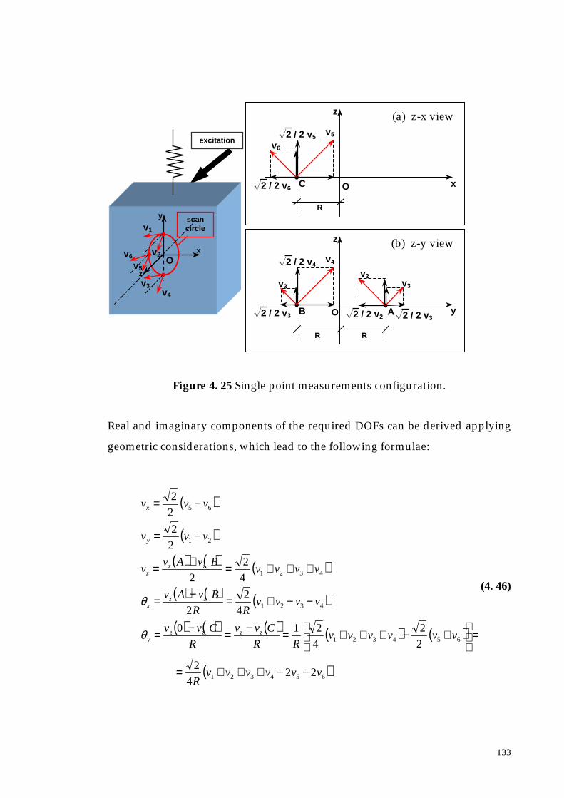
133

Figure 4. 25 Single point measurements configuration.

Real and imaginary components of the required DOFs can be derived applying

geometric considerations, which lead to the following formulae:

( )

( )

( ) ( ) ( )

( ) ( ) ( )

( ) ( ) ( ) ( ) ( )

( )654321

654321

4321

4321

21

65

224

2

2

2

4

210

4

2

2

4

2

2

2

2

2

2

vvvvvvR

vvvvvvRR

Cvv

R

Cvv

vvvvRR

BvAv

vvvvBvAv

v

vvv

vvv

zzzzy

zzx

zzz

y

x

−−+++=

=

+−+++=−=−=

−−+=−=

+++=+=

−=

−=

θ

θ(4. 46)

scancircle

x

y

z

excitation

v1

v2

v4

v3

v5

v6 O

C O

v6

v5

¥2 / 2 v6

¥2 / 2 v5

z

x

R

(a) z-x view

B O

v3

v4

¥2 / 2 v3

¥2 / 2 v4

z

y

R

A

v2

¥2 / 2 v2

R

v3

¥2 / 2 v3

(b) z-y view

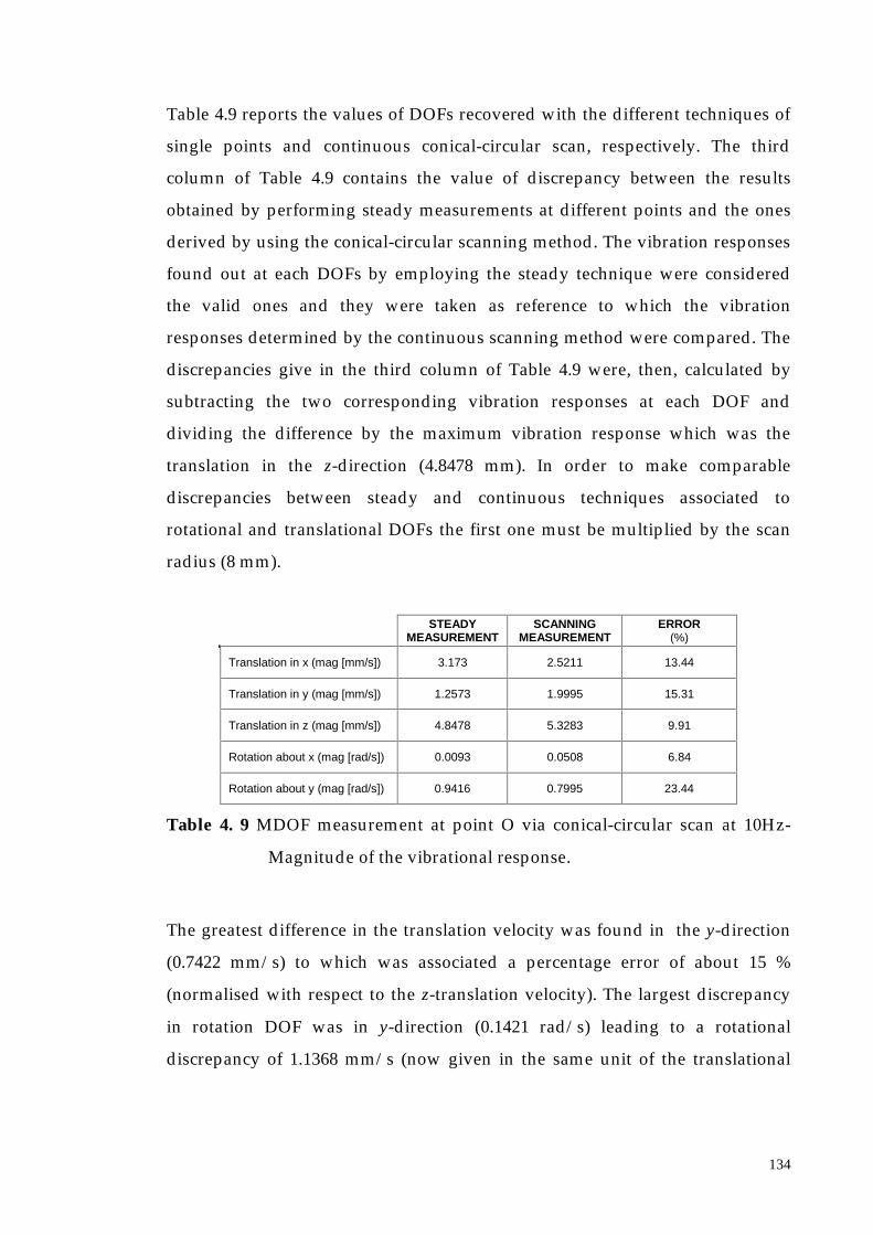
134

Table 4.9 reports the values of DOFs recovered with the different techniques of

single points and continuous conical-circular scan, respectively. The third

column of Table 4.9 contains the value of discrepancy between the results

obtained by performing steady measurements at different points and the ones

derived by using the conical-circular scanning method. The vibration responses

found out at each DOFs by employing the steady technique were considered

the valid ones and they were taken as reference to which the vibration

responses determined by the continuous scanning method were compared. The

discrepancies give in the third column of Table 4.9 were, then, calculated by

subtracting the two corresponding vibration responses at each DOF and

dividing the difference by the maximum vibration response which was the

translation in the z-direction (4.8478 mm). In order to make comparable

discrepancies between steady and continuous techniques associated to

rotational and translational DOFs the first one must be multiplied by the scan

radius (8 mm).

STEADYMEASUREMENT

SCANNINGMEASUREMENT

ERROR(%)

Translation in x (mag [mm/s]) 3.173 2.5211 13.44

Translation in y (mag [mm/s]) 1.2573 1.9995 15.31

Translation in z (mag [mm/s]) 4.8478 5.3283 9.91

Rotation about x (mag [rad/s]) 0.0093 0.0508 6.84

Rotation about y (mag [rad/s]) 0.9416 0.7995 23.44

Table 4. 9 MDOF measurement at point O via conical-circular scan at 10Hz-

Magnitude of the vibrational response.

The greatest difference in the translation velocity was found in the y-direction

(0.7422 mm/s) to which was associated a percentage error of about 15 %

(normalised with respect to the z-translation velocity). The largest discrepancy

in rotation DOF was in y-direction (0.1421 rad/s) leading to a rotational

discrepancy of 1.1368 mm/s (now given in the same unit of the translational

135

DOF). The percentage error is now, then, much higher, specifically of about 23

%.

Concerning the phase the maximum difference was 1.49° (translation in y-

direction) and all the phase responses and associated errors are reported in

Table 4.10.

STEADYMEASUREMENT

SCANNINGMEASUREMENT

ERROR(º)

Translation in x (phase º) 53. 87 55.29 1.42

Translation in y (phase º) -128.88 -130.37 1.49

Translation in z (phase º) -125.77 -124.81 0.96

Rotation about x (phase º) -119.92 -121.13 1.21

Rotation about y (phase º) 53.81 54.44 0.63

Table 4. 10 MDOF measurement at point O via conical-circular scan at 10Hz -

Phase of the vibrational response.

Errors can be due to the difficulties related to the setting of the single point

measurements. In fact, positioning the laser beam accurately in the different

directions required a major effort and it was difficult to guarantee that the laser

line-of-sight formed with the test specimen surface angles was exactly 45°.

From Table 4.10 it is possible to observe that the phase assumed approximately

the same value for each DOF, or it is shifted by 180°. This happens for the

special, but common, case where the mode shape is real, so that imaginary and

real components of Vx , Vy , Vz , Θx and Θy are all in the same ratio. Therefore, the

(temporal) phase angle, which is the inverse of the tangent of this ratio, will be

such that motion in all DOFs is in phase (or 180° out of phase).

136

4.6. Calibration of Continuous Scanning Techniques

4.6.1 Mirror Calibration

As emphasised in Section 4.1, a mirror calibration must be performed a priori in

order to derive the delay associated with these mechanical devices, together

with the rotors which drive them. In practice the delay is due to the global

inertia of both the mirror and the rotor.

In fact, considering the horizontal mirror, which moves the beam in the x-

direction, it is possible to show that, the sinewave, x(t), produced by the

software piloting the electronic card, whose output drives the mirror is

( ) ( )tVtx Ωπ2sin= (4. 47)

where V is the amplitude in volts and Ω is the scan frequency in Hz. Also if the

laser mirror is fed by x(t), the real position of the laser spot on the structure

depend on several others parameters associated to the chain of devices presents

in between the output of the electronic board and the scanning system.

Following each step of the process through which the driving signal passes, the

spot position can be related to x(t). The analog output of the electronic board,

x(t), is sent to the laser scanner placed in the laser head via an interface or

Analog-Digital converter which generates discrete data. The galvanometer

optical scanners are then driven by discrete voltages, which control the angular

movement of the mirror, α(t):

( ) ( )ϕπα += tVAt Ω2sin (4. 48)

In this relationship A represents the static sensitivity of the scanners and it is

expressed in (rad/V), being a ratio between mirror angle and driving signal,

137

while ϕ is the angular delay due to the scanner system inertia. It is worth noting

that if the interface produces discrete data, the mirrors are moving following a

typical ‘staircase’, but this stepwise characteristic is heavily filtered out by the

mirror inertia for the amplitudes and scan speeds commonly used. The angular

position of the mirror may be then related to the scanning plane coordinate

which defines the laser spot position on the target specimen by a geometrical

parameter, B, which depends on the mirrors’ position in the laser head and on

the optics characteristics, as the separation distance of the two mirrors surface

in the direction of the laser beam. The laser spot coordinate will be:

( ) ( )ϕπ += tVBAtx Ω2sin (4. 49)

where B is in mm/rad.

In Section 4.2, an ideal situation was assumed where the mirrors were not

subjected to any delay and the position of the laser spot was supposed to be,

simply:

( ) ( )tltxIDEAL Ωπ2sin= (4. 50)

l being the scan length. In order to make Equations (4.49) and (4.50) agree, and

to render Equation (4.50) general the parameters A, B and ϕ must be determined

a priori by calibration. Knowing the applied voltage V, the length of the scan on

the structure can be derived; although the amplitude calibration is not

important since a straight-line scan length is easily determined approximately

simply by using a scale on the scanned surface (idem for the radius on a circular

scan), see reference [36] and [40].

Instead what is necessary to determine exactly is the angular delay, which

defines the true position of the laser spot along the scan line or circle. Setting

ϕ at the value derived by calibration the start point of the continuous scan is the

point (called start point) marked in Figures 4.6, 4.9, 4.11, 4.20 for the different

138

situations (linear scan, circular scan, conical scan, conical - circular scan

respectively). It is possible to demonstrate that the mirror delay depends only

on the scan velocity because, considering the mirror together with its mounting

rotor as a rigid body with moment of inertia with respect to the rotation axis J,

the kinetic energy with which it reacts, when a rotational motion is imposed on

it, is:

2

2

1 ΩJT = (4. 51)

where Ω is the imposed scan speed. Then, a calibration process can be

performed varying only the scan speed, i.e. the rotation velocity of the mirror.

For each frequency a phase or time delay can be determined. This quantity will

be recovered by adjusting the relative phase of the LDV output time history and

the mirror signal, in order to make them perfectly in phase to each other, see

Figure 4.26.

Figure 4. 26 LDV output signal before and after applying the mirror delay

correction.

It can be noticed that in the second plot of Figure 4.26 the LDV output and the

sinewave indicating the laser spot position are in phase with each other because

the mirror delay correction has been performed. When this condition is reached,

both the real and the imaginary parts of the upper and lower sidebands of the

0 0.1 0.2 0.3 0.4 0.5

-3

-2

-1

0

1

2

3

Time (sec)0 0.1 0.2 0.3 0.4 0.5

-3

-2

-1

0

1

2

3

Time (sec)

Tim

e hi

stor

ies

(V)

Tim

e hi

stor

ies

(V)

139

LDV output, obtained by a line scan measurement, are equal but opposite in

sign, as was highlighted in Section 4.2. Following this recurrence, the calibration

can be preformed on the basis of a line scan test.

It is preferable to calibrate using a test piece, such as the cube used for the

demonstrations described in the previous sections, for which a pure rocking

mode can be established. The test set-up was the same as the one shown in

Figure 4.5 and the structure excitation was again at 158 Hz. To calibrate the x-

mirror, a small horizontal straight line scan of length of 18 mm was performed

by driving the x-scanning system with a sinewave of suitable amplitude and of

frequency set at different values (0.5, 0.7, 1, 1.5, 2, 3, 4, 5, 10, 15, 20, 25, 30 Hz).

The LDV acquisition was triggered with the mirror signal, i.e. when the

scanning sinewave passes through zero with positive slope and, therefore, if

there was no delay in the mirror, the laser spot position should follow perfectly

the driving signal and the LDV time history should be completely in phase with

the mirror signal, as shown in the right-hand plot in Figure 4.26. Then, by

performing a curve-fit of the LDV output, the derived sidebands’ complex

components must realise the recurrence above mentioned. In practice, this

recurrence does not happen at any scan speed imposed to the mirror driving

the laser beam, because a delay exists also at low frequencies. The LDV output

is then shifted by a phase angle, α, until its complex sideband components are

equal and opposite in sign: this angle represents the mirror delay. From this, the

time delay is simply deducible by dividing it by (360 Ω ), Ω being the scan

frequency.

The x-mirror delay values are listed in Table 4.11 and plotted against the scan

speed in Figure 4.27.

140

SCAN FREQUENCY(Hz)

PHASE ANGLE(°)

TIME DELAY(sec)

0.5 2.28 1.2667 10-2

1 2.77 7.6944 10-3

2 3.95 5.4861 10-3

3 5.14 4.7593 10-3

4 4.32 3.0000 10-3

5 6.33 3.5167 10-3

10 7.52 2.0889 10-3

15 10.83 2.0056 10-3

20 12.8 1.7778 10-3

25 14.32 1.5911 10-3

30 16.81 1.5565 10-3

Table 4. 11 Phase angles and relative time shifts associated to the x-mirror

delay.

Figure 4. 27 Phase angles and relative time shifts plotted against the scan

frequency.

The interpolation line shown in the first plot of Figure 4.27 is determined by a

least-squares method; if the line is

Ωbay += (4. 52)

the line coefficients are

0 5 10 15 20 25 300

10

20

30

40

50

60

70

80

90

Scan Frequency (Hz)

Pha

se A

mgl

e (d

eg)

Interpolation Line

0 5 10 15 20 25 300

0.01

0.02

0.03

0.04

0.05

0.06

0.07

0.08

0.09

0.1

Scan Frequency (Hz)

Tim

e D

elay

(sec

)

141

( ) ( )2222

2

and∑∑

∑∑∑∑∑

∑∑∑∑−

−=

−

−=

ii

iiii

ii

iiiii

n

nb

na

ΩΩ

ΩΩ

ΩΩ

ΩΩΩ αααα (4. 53)

where Ω is the scan frequency vector and α the phase angle vector consisting of

n elements (which are 11, see Table 4.11). The same procedure was conducted to

calibrate the y-mirror and Table 4.12 and Figure 4.28 show its behaviour.

SCAN FREQUENCY(Hz)

PHASE ANGLE(°)

TIME DELAY(sec)

0.5 2.68 1.4889 10-2

1 4.77 1.3250 10-2

2 5.95 8.2639 10-3

3 7.14 6.6111 10-3

4 4.32 3.0000 10-3

5 6.50 3.6111 10-3

10 5.42 1.5056 10-3

15 8.83 1.6352 10-3

20 9.05 1.2569 10-3

25 9.92 1.1022 10-3

30 12.49 1.1565 10-3

Table 4. 12 Phase angles and relative time shifts associated to the y-mirror

delay.

Figure 4. 28 Phase angles and relative time shifts plotted against the scan

frequency.

Comparing Table 4.11 and Table 4.12, it is possible to deduce that the x-mirror

is more sensitive to the scan speed increase: the delay increases faster, i.e. the

0 5 10 15 20 25 300

10

20

30

40

50

60

70

80

90

Scan Frequency (Hz)

Pha

se A

ngle

(deg

)

Interpolation Line

0 5 10 15 20 25 300

0.01

0.02

0.03

0.04

0.05

0.06

0.07

0.08

0.09

0.1

Scan Frequency (Hz)

Tim

e D

elay

(sec

)

142

slope of the line interpolating the angle values is greater by comparison with

the one associated with the y-mirror calibration values, see Figure 4.29.

0 5 10 15 20 25 300

10

20

30

40

50

60

70

80

90

Scan Frequency (Hz)

Inte

rpol

atio

n Li

ne (d

eg)

x-mirrory-mirror

Figure 4. 29 Comparison of phase angles associated to the delay of both the

mirrors.

The discrepancy between the two mirrors is unexpected, since the mirrors are

ostensibly identical and so their inertias should be alike. This difference can be

explained taking into account uncertainty sources connected to the hardware

systems as non-linearity of the galvanometer device and the position sensor

which constitutes the feedback control system, optical and mechanical

inaccuracy (i.e. mirrors misalignment) and electronic problems (such as errors

in D/A conversion).

In addition to the previous general calibration, additional ones must be

conducted for each scanning technique; some can be avoided, as the line scan

length derivation, since they can be easily determined by direct measurement,

but some are indispensable.

4.6.2 Line-Scan Calibration

In spite of what has been said above, however, it is difficult to measure the scan

line length to, say, 1% by this means. The angle of vibration can then be derived

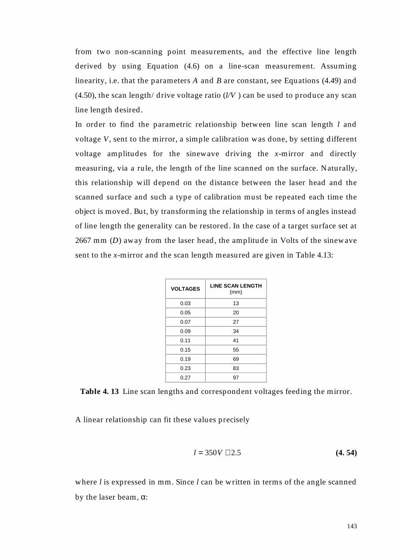
143

from two non-scanning point measurements, and the effective line length

derived by using Equation (4.6) on a line-scan measurement. Assuming

linearity, i.e. that the parameters A and B are constant, see Equations (4.49) and

(4.50), the scan length/drive voltage ratio (l/V ) can be used to produce any scan

line length desired.

In order to find the parametric relationship between line scan length l and

voltage V, sent to the mirror, a simple calibration was done, by setting different

voltage amplitudes for the sinewave driving the x-mirror and directly

measuring, via a rule, the length of the line scanned on the surface. Naturally,

this relationship will depend on the distance between the laser head and the

scanned surface and such a type of calibration must be repeated each time the

object is moved. But, by transforming the relationship in terms of angles instead

of line length the generality can be restored. In the case of a target surface set at

2667 mm (D) away from the laser head, the amplitude in Volts of the sinewave

sent to the x-mirror and the scan length measured are given in Table 4.13:

VOLTAGES LINE SCAN LENGTH(mm)

0.03 13

0.05 20

0.07 27

0.09 34

0.11 41

0.15 55

0.19 69

0.23 83

0.27 97

Table 4. 13 Line scan lengths and correspondent voltages feeding the mirror.

A linear relationship can fit these values precisely

5.2350 += Vl (4. 54)

where l is expressed in mm. Since l can be written in terms of the angle scanned

by the laser beam, α:

144

αα DDl 2tan2 == (4. 55)

α being small, due to the fact that D >> l, the more general relationship will

become:

026.0758.32

5.2

2

350 +=+= VD

VD

α (4. 56)

where α is expressed in degrees.

Equation (4.56) was found to be valid also for the y-mirror, and consequently

for circular scan.

As already stated, this calibration method must be repeated every time the

scanning LDV settings (specifically, the distance from the object) are changed.

However, the procedure is general and it is suitable for all the scanning laser

systems available in commerce.

4.6.3 Circular-Scan Calibration

As for a line scan, approximate scan circles can be arrived at by eye, adjusting

the x- and y-axis drive voltages and relative phase to suit. For best accuracy,

however, equal scan amplitudes should be set for both mirrors using the

straight-line scan procedure.

The phase shift in the mirror drive may not be exactly the same for both

mirrors. One method of countering this is to set the relative phase between x

and y mirror drives to produce a single diagonal line. The y-axis drive voltage is

then shifted by exactly 90° to achieve a circle.

It is assumed in the analysis carried out above that the direction of scan is

clockwise on the surface, viewed from the laser head. This can be conveniently

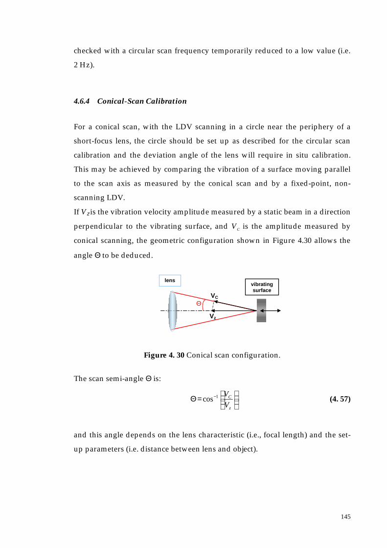
145

checked with a circular scan frequency temporarily reduced to a low value (i.e.

2 Hz).

4.6.4 Conical-Scan Calibration

For a conical scan, with the LDV scanning in a circle near the periphery of a

short-focus lens, the circle should be set up as described for the circular scan

calibration and the deviation angle of the lens will require in situ calibration.

This may be achieved by comparing the vibration of a surface moving parallel

to the scan axis as measured by the conical scan and by a fixed-point, non-

scanning LDV.

If Vz is the vibration velocity amplitude measured by a static beam in a direction

perpendicular to the vibrating surface, and VC is the amplitude measured by

conical scanning, the geometric configuration shown in Figure 4.30 allows the

angle Θ to be deduced.

Figure 4. 30 Conical scan configuration.

The scan semi-angle Θ is:

= −

z

C

V

V1cosΘ (4. 57)

and this angle depends on the lens characteristic (i.e., focal length) and the set-

up parameters (i.e. distance between lens and object).

Θ

Vz

vibratingsurface

VC

lens

146

4.7. Conclusions

Continuous scanning techniques for determining MDOF vibrational responses

have been described mathematically, simulated numerically and tested

experimentally on a simple laboratory specimen (an aluminum cube made for

the purpose) in this chapter.

The continuous scanning techniques have been applied the so-called ‘short

scan’ methods, where the laser is made to scan on different paths as (i) lines, (ii)

circles, (iii) cones. Different MDOF vibration measurements can, then, be

performed using the suitable type of scan:

1. Linear Scan for one translational and one angular DOFs recovery;

2. Circular Scan for one translational and two angular DOFs recovery;

3. Conical Scan for three translational DOFs recovery;

4. Conical-Circular Scan for three translational and two angular DOFs

recovery.

The accuracy of the CSLDV techniques have been studied by comparing the

experimental results with ones obtained by single-point measurements. The

greatest discrepancies found between the results from the two techniques were

around 10%. For a detailed comparison analysis, see Section 4.2 (short line

scans), Section 4.3 (small circular scans), Section 4.4 (conical scans) and Section

4.5 (conical-circular scans).

Problems related to the continuous scanning methods employed in the short

scan fashion were treated in detail, by giving the most emphasis to the mirror

scanning system calibration. Some practical applications on industrial case

study will be examined with particular detail in Section 7.2 in Chapter 7.

Chapter 5 Continuous ScanningTechnique Applied toOperational Deflection ShapeMeasurements

5.1. Introduction

This chapter investigates continuous scanning techniques when scans are

performed over long straight-lines, large circles or whole 2D surfaces (see Table

4.1, Chapter 4, for the schematic summary). In order to follow the development

of the chapter, a map of its structure can be helpful as a breakdown of the

treated topics.

First the linear scan is addressed and the analysis is split as shown in Table 5.1.

The second topic is the circular scan: its treatment breakdown is illustrated in

Table 5.2. Subsequently, in Section 5.5 the two-dimensional scan (area scan),

whose topics are summarised in Table 5.3, is described. The last major subject is

the Modal Analysis on FRF data acquired by using the continuous area

scanning technique and its breakdown is depicted in Table 5.4.

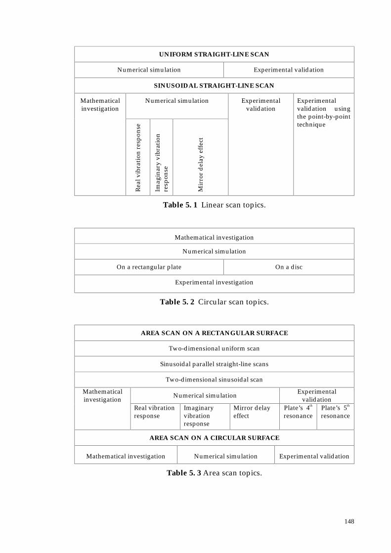
148

UNIFORM STRAIGHT-LINE SCAN

Numerical simulation Experimental validation

SINUSOIDAL STRAIGHT-LINE SCAN

Numerical simulationMathematicalinvestigation

Rea

l vib

rati

on r

espo

nse

Imag

inar

y vi

brat

ion

resp

onse

Mir

ror

del

ay e

ffec

t

Experimentalvalidation

Experimentalvalidation usingthe point-by-pointtechnique

Table 5. 1 Linear scan topics.

Mathematical investigation

Numerical simulation

On a rectangular plate On a disc

Experimental investigation

Table 5. 2 Circular scan topics.

AREA SCAN ON A RECTANGULAR SURFACE

Two-dimensional uniform scan

Sinusoidal parallel straight-line scans

Two-dimensional sinusoidal scan

Numerical simulation Experimentalvalidation

Mathematicalinvestigation

Real vibrationresponse

Imaginaryvibrationresponse

Mirror delayeffect

Plate’s 4th

resonancePlate’s 5th

resonance

AREA SCAN ON A CIRCULAR SURFACE

Mathematical investigation Numerical simulation Experimental validation

Table 5. 3 Area scan topics.

149

MODAL ANALYSIS ON CSLDV FRFs DATA

Experimental modal analysis on the GARTEUR structure

Concluding remarks

Table 5. 4 Modal analysis on CSLDV FRFs data.

5.2. Measurement Methodology

A number of new ODS measurement techniques are described here, applying

the LDV scanned continuously over the surface of a sinusoidally-excited

structure. Under these conditions, the LDV output is an amplitude-modulated

sinewave from which the ODS, defined along the scan pattern, can be derived.

If the scan speed is uniform, the structure’s deflection shape can be directly

recovered by demodulating the LDV output time history. Actually, in this case,

the ODS is the envelope of the modulated LDV output signal. Otherwise, if the

laser beam is scanning sinusoidally, the LDV output spectrum can be analysed

in the frequency domain where it is represented by spectral lines centered on

the excitation frequency and spaced at multiple of the scan frequency. It is

worth noting that the number of terms comprising the LDV output spectrum

will be limited only if the ODS is smooth, i.e. if no discontinuities occur within

the vibration pattern where the laser is scanning. The sideband amplitudes give

a series of coefficients for the mode shape defined along the scan path: Fourier

coefficients for a circular scan or, via a simple transform, polynomial

coefficients for a sinusoidal straight line or area scan.

Demodulation techniques will be addressed in this chapter for line and area

scans at uniform speed, obtained by driving one or both at the scanning mirrors

respectively, by triangular waveforms. Frequency-domain techniques described

here are straight-line and circular scans, in which the scanning mirrors, again

one or both of them, are fed with sinewaves. Applications of circular scans to

the measurement of vibration of rotating discs are included. The use of line scan

theory can then be widened to recover of two-dimensional ODSs that can be

150

produced either from sets of straight-line scans or by performing a continuous

two-dimensional sine scan.

Previous works done in the CSLDV technique can be found in literature, see

references [16], [41] and [42] for straight-line scanning techniques. As

concerning 2-dimensional ODS measurement previous developed works are

described in references [15] and [17]. [39]. For modal analysis on FRF data

measured by CSLDV see references [39] and [19].

All the continuous scanning techniques employed in ODS recovering involve

sinusoidal excitation of the structure: experimental structures are excited by

sinusoidal input forcing so that the response at any point, measured at any

direction, is also sinusoidal at the same frequency, assuming the structure to be

effectively linear. The response, in general, is not in-phase with the force and it

does not necessarily have a uniform phase across the scan.

By directly applying these techniques, ODSs can be determined, these being

forced vibration patterns of the structure and not natural or “normal” mode

shapes. In fact, ODSs have contributions from more than one natural mode,

each with a different mode shape and phase-shift between the motions in all the

measurement locations (if the mode is real, all the points are in phase with each

other or 180° out of phase). A perfectly real ODS is normally produced on

undamped structures, however, in the case of damped structures, it is possible

to generate a real ODS if a multiple-input normal mode test is made. However,

in practice, lightly-damped structures, vibrating at a frequency close to the

natural frequency, assume nearly real ODSs which are normally the same as the

undamped natural mode shapes. In other cases, particularly if there are close

natural frequencies, or with heavily-damped structures, an ODS may be

markedly complex. If frequency responses are available, modal analysis may be

applied, a process which eliminates the contributions from extraneous modes,

extracting the natural mode shapes.

151

5.3. Analysis of a Linear Scan

5.3.1 Introduction

This technique involves a one-dimensional scan along a line that can be swept

by the laser moving at a uniform speed or sinusoidally-varying. The first option

is the so-called demodulation method which is straightforward to apply since

the ODS along the line is directly derived by demodulating the LDV output in

the time domain. The second option is to work in the frequency domain and

employs a sinusoidal linear scan in order to avoid the discontinuities at the end

of each scan that otherwise occur whenever the scan direction reverses. In fact,

even if the scan speed is constant along the scan line, when the laser beam

changes direction it suddenly passes from a positive velocity to a negative one,

causing a discontinuity. In contrast, if the scan is sinusoidal, the velocity of the

laser beam reduces smoothly to zero at the ends of the scan line. This

arrangement allows it to work with Fourier spectra of the LDV output.

However, with the uniform rate scan, the LDV signal in the frequency domain

does not contain any useful information.

5.3.2 Uniform straight-line scan

5.3.2.1 Numerical Simulation

Firstly, the method applying the continuous scan at a uniform rate is studied

mathematically and simulated in order to foresee how a simple structure will

behave during vibration tests. An experimental case will be then analysed.

A simple specimen can be considered as a free-free beam undergoing a

sinusoidal vibration at a frequency ω, see Figure 5.1. The vibration, which is

expressed here as velocity in the z-direction, perpendicular to the beam surface

152

nominally in the x, y plane, and measured at a point x along the scan line, will

be:

txVtxVtxv IRz ωω sin)(cos)(),( += (5. 1)

VR and VI being the real and imaginary components of the vibration, relating to

some datum that is usually the input force.

If the laser beam is scanned continuously at a uniform rate, v, at each instant, t,

the position of the laser spot along the scanned line, can be represented by the

quantity x = vt, so that the vibration velocity can be considered as a function of

time only.

Figure 5. 1 Laser linear scan on the beam.

Assuming that the beam is vibrating at the second natural frequency, the

second mode shape can be simulated following the Timoshenko theory on

simple beam transverse vibrations theory for free-ends conditions, [43]. The

solution of the motion equation is:

( ) ( ) ( )kxkxCkxkxCxV sinhsincoshcos 21 +++= (5. 2)

Applying the boundary conditions for the free-ends beam, assumed to have a

unitary length of 1 m, constants k and the ratio C1 / C2 are derived as:

y

x

LINE SCAN

BEAM

153

99922.0

853.7

2

1 −=

=

C

C

k

The second bending mode shape is then described by Equation (5.2), by

introducing the constant values on it and it is visualised along the length of the

beam in Figure 5.2. Assuming that the mode is completely real, i.e. that VR(x) =

V(x) and VI (x) = 0, Equation (5.1) can be written as:

( )[ ]( )t

xxxxtxVtxvz

22cos

853.7sinh853.7sin853.7cosh853.7cos99922.0cos)(),(

πωω

×+++−==

(5. 3)

where ω2 is the natural frequency, which can be derived from the simple beam

theory.

A

EIk

ρπω

2

22

2 = (5. 4)

EI being the flexural rigidity of the beam, A its cross-section area, and ρ the

mass density of the material. Considering a beam of cross-section 0.005×0.05 m,

with the larger dimension in y-direction, and made of steel, the flexural rigidity

will be 114.58 Nm2 and the mass density 7810 kg/m2. The natural frequency

can therefore be calculated: ω2 = 472.43 Hz.

The beam position, x, depends on time, t, according to the following

relationship:

tlvtx Ω2== (5. 5)

where Ω is the scan frequency and l the beam length, i.e. within a complete scan

period the beam will be swept twice forward and backward. Substituting

154

Equation (5.5) in Equation (5.3), the vibration velocity can be expressed in

function of time only:

( ) ( )[ ] ( ) ( ) tf

tttttvz

2cos

853.72sinh853.72sin853.72cosh853.72cos99922.0)(

×⋅+⋅+⋅+⋅−= ΩΩΩΩ

(5. 6)

where the beam length is normalised to 1.

Figure 5. 2 Second mode deflection shape.

Deriving vz from Equation (5.3), with ω2 = 472.43 Hz, and assuming the laser

beam to scan at a frequency, Ω, of 0.5 Hz, a time signal is found, and this is the

signal at the output of the LDV whose laser beam is scanning along the length

of the beam. The vibration time vector is shown in Figure 5.3, where the

envelope modulation, i.e. the mode shape, is emphasised.

L

z

x

155

0 0.2 0.4 0.6 0.8 1time (s)

v z(t) (

m/s

)

Figure 5. 3 LDV output modulated by the bending mode shape of the

beam (red line).

From the simulation it can be deduced that the ODS may be obtained by

demodulating the SLDV output signal. A convenient method to perform the

demodulation is simply to multiply the LDV output signal alternately by

cosine and sine waves at the excitation frequency.

ttVttVtVttVtttV

ttVttVtVtttVttV

IRIIR

IRRIR

ωωωωω

ωωωωω

2cos)(2

12sin)(

2

1)(

2

1sin)(cossin)(

2sin)(2

12cos)(

2

1)(

2

1cossin)(cos)(

2

2

−+=+

++=+ (5. 7)

If the scan speed is sufficiently slow, the signal components at the frequency 2ω

can be removed by using a low-pass filter and the real and imaginary

coefficients of the ODS can be derived in the time domain. The complex

vibration pattern is then obtained with a resolution that depends on the

sampling rate set during the acquisition and the scan rate. In practice, cross-talk

interference may occur at the excitation frequency, so it is convenient to set the

filter cut-off below this frequency value.

156

5.3.2.2 Experimental Validation

The uniform straight-line scanning technique can be applied experimentally by

driving the horizontal scanning mirror with a triangular wave so that the laser

beam will sweep along a straight line alternately in opposite directions with

uniform speed.

Software for the control, data-acquisition and post processing has been

developed in LabVIEW in order to have in output of it directly the ODS real and

imaginary components. This routine is composed of several sub-routines,

consisting of:

- a control program which generates the sinewave to be sent to the shaker

for the structure’s excitation. The excitation frequency and amplitude are

the only parameters that are to be set (see Appendix A.1.1 for the control

panel of the LabVIEW program driving the shaker).

- a control program used to produce the triangular wave driving the

scanning mirror. The amplitude of the waveform should be set according

to the length of the scan required and the scan frequency must be

carefully chosen. It has to be sufficiently slow with respect to the

excitation frequency (see Appendix A.1.2 for the control panel of the

LabVIEW program driving the mirrors).

- an acquisition program where the sample rate chosen must follow the

Nyquist theorem and the number of samples to acquire must be set so

that the time length of the signal coincides exactly with the scan period.

In this situation the mode shape will be swept twice (see Appendix A.1.3

for the control panel of the LabVIEW program used for the acquisition).

- a post-process program which performs the multiplication of the signal

acquired by sine and cosine at the excitation frequency and applies a low

pass filter whose threshold frequency must be fixed (see Appendix A.1.4

for the control panel of the LabVIEW program performing the

demodulation procedure).

157

The last part of the program can also be performed using a Matlab routine,

leaving to the LabVIEW software only the tasks of control and acquisition.

An experimental example has been carried out using as a measurement

specimen a free-free steel beam, 32 mm wide, 10.05 mm thick and 1000 mm

long. Measurements involved a half-scan, from the centre to one end, for modes

1, 3, and 5 found experimentally at 58 Hz, 311 Hz and 766 Hz, respectively.

For the first ODS recovery, the scan frequency was set at 0.5 Hz and, since the

sample rate was chosen to be 1000 Hz, the LDV output signal was sampled with

2000 samples in order to have a time window as long as the scan period (i.e. 2

s). The time signal acquired is shown in Figure 5.4 while Figure 5.5 depicts the

in-phase and out-of-phase ODS components referred to an initial datum, which

is the phase of the vibration when its real component is maximum. Using this

procedure the phase is adjusted to minimise the output to give the effectively

zero imaginary part of the ODS and then, shifted by π/2, to give the real

component. The low-pass-filter frequency was fixed at 20 Hz.

0 0.5 1 1.5 2s

V

Figure 5. 4 LDV output signal (blue) and mirror driving signal (red).

158

Figure 5. 5 In-phase and out-of-phase components of the ODS at 58 Hz.

The same procedure was followed on the ODSs recovered at the higher

frequencies of 311 and 766 Hz. In-phase and out-of-phase components are

depicted in Figures 5.6 and 5.7.



scan length

mid

tip

scan length

mid

tip

scan length

tip

159

A comparison can be made between ODSs recovered by demodulation and

analytical mode shapes derived by Timoshenko theory, whose frequencies are

calculated from Equation (5.4), knowing the constant k. Table 5.5 summarises

values of k and natural frequencies ω, for modes 1, 3 and 5 the factor A

EI

ρ

assuming the value of 16.08 m2/s, with E and ρ the Young modulus and the

mass density of steel.

MODE NUMBER k (m-1) ω (Hz)EXPERIMENTAL FREQUENCY

(Hz)

1 4.730 57.28 58.00

3 10.996 309.57 311.00

5 17.279 764.42 766.00

Table 5. 5 Analytical natural frequencies.

Mode shapes are established by Equation (5.2) using for each mode the

corresponding constant k and ratio C1 /C2 . The vibration velocity will then be:

( )( )

( )xxxxxv

xxxxxv

xxxxxv

z

z

z

279.17sinh279.17sin9999999329.0279.17cosh279.17cos)(

996.10sinh996.10sin999966878.0996.10cosh996.10cos)(

73.4sinh73.4sin9822.073.4cosh73.4cos)(

+−+=+−+=

+−+=(5. 8)

which are for modes 1, 3 and 5 respectively. They are plotted together with the

ODSs derived by demodulation at the same frequency as Figures 5.8, 5.9 and

5.10 show.

It can be noticed that nodal points are coincident for each mode and the relative

ODSs since all of them are mostly real; on the other hand the amplitude is

different because the ODS represent the absolute deformed shape dependent on

the actual force applied. On the contrary, the mode shape is not dependent on

the measurement system being derived from an FRF namely the structure

vibration velocity divided by the input force.

160

Figure 5. 8 Analytical mode shape and ODS at 58 Hz.



0 0.1 0.2 0.3 0.4 0.5-3

Beam Length

Vib

ratio

n A

mpl

itude

Analytical Mode ShapeODS from Demodulation

0

(V)

5

0 0.1 0.2 0.3 0.4 0.5-4

Beam Length

Vib

ratio

n A

mpl

itude

Analytical Mode ShapeODS from Demodulation

0

(V)

4.5

0 0.1 0.2 0.3 0.4 0.5Beam Length

Vib

ratio

n A

mpl

itude Analytical Mode Shape

ODS from Demodulation

0

(V)

-2

2.5

161

A disadvantage of the uniform-rate straight-line scans is the instantaneous

reversal in velocity at each end of the sweep that taxes the capability of the

mirror drive electronics but, more importantly, provokes distortions near the

scan end-points. There are no such sudden reversals with a sinusoidal straight-

line scan but distortions can still occur, and may be particularly difficult to

detect.

5.3.3 Sinusoidal straight-line scan

5.3.3.1 Mathematical Investigation

The mode shape contributions VR (x) and VI (x) in Equation (5.1) can be

expanded as spatial Fourier series, along the scan line. However, if the laser

beam moves at uniform speed, difficulties can arise during the Fourier

transform because of the discontinuities at the end of the scan, where the scan

direction reverses. The end-point discontinuities can be avoided by employing

a sinusoidal linear scan so that the scan velocity reduces smoothly to zero at

these ends.

Assuming the complex operational deflection shape of the beam to be a smooth

deflection pattern, it can be described as a polynomial which is, in the general

case, of pth order. The vibration in the z-direction will consist then of two

components, real and imaginary:

( )

( ) ∑

∑

=

=

=

=

p

n

nInI

p

n

nRnR

xVxV

xVxV

0

0 (5. 9)

x being the normalised position vector representing all the points along the line.

It goes from –1 to 1 considering the zero position the center of the line and

162

normalising at 2 its total length. VRn is the nth polynomial coefficient describing

the velocity pattern along the line. The vibration can be written following the

principle of Equation (5.1):

( ) ( ) ( )∑∑==

+=p

n

nIn

p

n

nRnz txVtxVtxv

00

sincos, ωω (5. 10)

ω being the angular frequency of vibration. If the measurement points are

continuously scanned sinusoidally at frequency Ω along the line of length

normalised at 2, the instantaneous position of the laser spot over that line

would be represented by the sinewave of equation:

( ) ( )ttx Ωcos= (5. 11)

Consequently, Equation (5.10) becomes:

( ) ( ) ( ) ( ) ( )∑∑==

+=p

n

nIn

p

n

nRnz ttVttVtv

00

sincoscoscos ωω ΩΩ (5. 12)

Expanding out trigonometrically, multiple terms arise at frequencies (ω ± nΩ ),

which are called upper and lower sidebands. Their value, in magnitude and

phase, is the same for both the real and imaginary components, i.e. both the real

and the imaginary Fourier spectra are symmetrical with respect to the central

frequency or excitation one. The vibration can be expressed as:

( ) ( ) ( )[ ] ( ) ( )[ ]∑∑=

±=

± ±+±=p

nnI

p

nnRz tnAtnAtv

00

sincos ΩΩ ωω (5. 13)

AR0 being the spectrum component at the excitation frequency ω and AR±1

the spectrum sidebands amplitude at (ω ± Ω ), and so on up to n = p. Deriving

163

the sideband coefficients AR ,6n from the polynomial coefficients VRn it can be

shown that AR ,- n = AR ,+ n , see below. Then Equation (5.13) becomes:

( ) ( )[ ] ( )[ ]∑∑==

±+±=p

nnI

p

nnRz tnAtnAtv

00

sincos ΩΩ ωω (5. 14)

After some manipulations the sideband coefficients, AR and AI, can be seen as

related to the corresponding polynomial coefficients, VR and VI, by a simple

matrix transform [T].

[ ] [ ] II

RR

ATV

ATV

==

(5. 15)

where, for 15th order polynomials, [T] is:

[ ]

−−

−−

−−−−

−−−−

−−−−−−

−−−−−−

−−−−−−−−

=

32768000000000000000

01638400000000000000

122880081920000000000000

05734404096000000000000

1843200266240204800000000000

078848012288010240000000000

140800033280056320512000000000

05376001382402560025600000000

57600019968056320115201280000000

01881607168022400512064000000

1209605824024640864022403200000

0313601680080003200960160000

1120072804400240011204008000

0196014401000640360160400

3002602201801401006020

0202020202020201

T

(5. 16)

164

The matrix can be derived simply by expanding the real or the imaginary

component of Equation (5.12). In fact, considering n = 0...3, for each value of n

the equation addends will be:

( )

( )[ ]

( )[ ] ( )

( )[ ] ( )[ ]tVt

Vnfor

tV

tV

nfor

tV

nfor

tVnfor

RR

RR

R

R

ΩΩ

Ω

Ω

±+±=

+±=

±=

=

ωω

ωω

ω

ω

cos8

33cos

83

cos2

2cos4

2

cos2

1

cos0

33

22

1

0

For a generic n it can be written, [44]:

( )[ ] ( )( )[ ] ( )( )[ ]

])([cos2

1..

..4cos2

2cos1

cos2 )1(

tnn

tnn

tnn

tnV

nRn

Ω

ΩΩΩ

±

−+

+−±

+−±

+±−

ω

ωωω

In the frequency domain the LDV output will, then, have components at the

usual frequencies with the following amplitudes, called A (as mentioned above

the spectral amplitudes at the frequencies (ω ± nΩ) are the same):

83

42

8

3

2

2

33

22

311

200

RR

RR

RRR

RRR

VAat

VAat

VVAat

VVAat

=±

=±

+=±

+=

Ω

Ω

Ω

ω

ω

ω

ω

which can be written as

165

=

3

2

1

0

3

2

1

0

81000

04100

8302

10

02101

R

R

R

R

R

R

R

R

V

V

V

V

A

A

A

A

The polynomial coefficients can be expressed in function of the spectral

amplitude only by inverting the matrix transform, which will then, coincide

with [T].

Note that the sensitivity to higher polynomial components diminishes rapidly

as n increases.


5.3.3.2.1 Real Vibration Response

The vibration velocity vz(t) can be simulated, assuming it is associated with the

same beam shown in Figure 5.1, where the LDV is now scanning sinusoidally

along the straight line. The beam is again supposed to vibrate at the second

natural frequency, i.e. 472.43 Hz as derived above. First, the beam vibration is

considered to be real (standing wave on the beam), later (subsection 5.3.3.2.2)

the complex case (travelling wave along the beam) will be analysed, where the

vibration along z consists of two components, real and imaginary ones.

The second flapwise bending mode is again simulated using the Timoshenko

theory and Equation (5.2) with values for k and C1 /C2 given. Considering the

real component only:

( ) xxxxxVR 853.7sinh853.7sin853.7cosh853.7cos99922.0)( +++−= (5. 17)

this can be approximated by a polynomial of, say, the 10th order.

166

( )424343

5647849106

21.23949.584.46450.1419.2

5870.1010.38972.392.25601.026.2−−−

−−−

+−−++

−−++−=

exxexxe

xxexxexxexVR (5. 18)

The vibration response assumes the form of a standing wave, i.e. nodal points

are spatially fixed, as shown in Figure 5.11.

( ) ( ) ( )( )texxexxex

xexxexxetxVtxv Rz

ωω

cos)21.23949.584.46450.1419.25870.10

10.38972.392.25601.026.2(cos,4243435

647849106

−−−

−−−

+−−++−

+−++−==

(5. 19)

Figure 5. 11 Vibration pattern at different time instants.

If the measurement points are continuously scanned sinusoidally at a

frequency of 10 Hz along the beam assumed to have a length of 2 m, the

velocity will depend on time only.

( ) ( ) ( ) ( )( ) ( ) ( )( ) ( ) ( )

( ) ( )tet

tette

ttet

tettetvz

43.4722cos)21.2102cos3949.5

102cos84.4102cos6450.14102cos19.2

102cos5870.10102cos10.3102cos8972.3

102cos92.2102cos5601.0102cos26.2(

4

24343

5647

849106

πππππ

ππππππ

−

−−

−

−−

+−

+−++

+−−+

++−=

(5. 20)

where ω = 472.43 Hz.

L

z

x- 1 + 1

167

Considering a time vector sampled at a sample rate of 10000 Hz at 100000

points the LDV output signal vz(t) can be plotted as in Figure 5.12.

0 0.05 0.1 0.15 0.2-2.5

-2

-1.5

-1

-0.5

0

0.5

1

1.5

2

2.5

Time (s)

Vel

ocity

(m/s

)

Figure 5. 12 Velocity response.

Looking at the spectrum of the LDV time signal, sideband components appear

at frequencies far apart from the excitation 472.43 Hz of 10 Hz. Their phases, as

expected, are 0° or 180°, because a structure vibrating in a real mode will have

all the points constituting it vibrating in-phase or in anti-phase with each other.

Figure 5.13 shows magnitude and phase of the spectrum of the velocity time

signal.

350 400 450 500 550 6000

0.2

0.4

0.6

0.8

Mag

nitu

de (m

/s)

350 400 450 500 550 600-200

-150

-100

-50

0

50

Frequency (Hz)

Pha

se (d

eg)

Figure 5. 13 Velocity spectrum.

168

The amplitudes of the spectrum at the components 472.43 ± n 10 Hz, for n = 0 ...

10 (the polynomial being of the 10th order) are associated with a conventional

sign of + if their phase is 0° and – if it is –180°. They can be converted again in

polynomial coefficients applying the matrix transformation [T] as in Equation

(5.15).

The vector A is measured directly from the spectrum at the precisely known

frequencies:

A = 8.26 e-4 0.4138 4.59 e-4 0.7239 1.80 e-4 -0.1570 4.44 e-5 0.0206 4.12 e-5

-0.0010 4.00 e-5 (m/s)

and applying the transformation (5.14) the vector VR is recovered as

VR = 1.81 e-4 -5.3944 0.0019 14.6380 -0.0202 -10.5600 0.0714 3.8562

-0.0919 -0.5396 0.0410 (m/s)

that compared with the initial values

VR = 2.21 e-4 -5.3949 -4.84 e-4 14.6450 0.0022 -10.5870 -3.10 e-4 3.8972

-2.92 e-4 -0.5601 2.26 e-6 (m/s)

shows a real error of:

err = 0.0007 0.0090 0.0445 0.1190 0.4156 0.4985 1.3300 0.7611 1.7100

0.3802 0.7600 %

The error is calculated as

1001

×−

=initialR

derivedRinitialR

V

VVerr (5. 21)

169

where VR initial 1 = - 5.3949 m/s, the reference value.

5.3.3.2.2 Complex Vibration Response

Now, the more general case of complex vibration is taken into analysis: the

beam’s second flapwise ODS is supposed to be composed of real and imaginary

components, VR (x) and VI (x), that can be approximated by two polynomial of

the 10th order:

( )

( )4578.06495.42832.33360.101198.33049.6

48.19277.12933.02472.00380.0

21.23949.584.46450.1419.2

5870.1010.38972.392.25601.026.2

2345

6478910

424343

5647849106

+−−++−

−++−−=+−−++

−−++−=

−

−−−

−−−

xxxxx

xexxxxxV

exxexxe

xxexxexxexV

I

R

(5. 22)

The ODS real and imaginary components are shown together in Figure 5.14. In

this case the vibration appears as a travelling wave that can be emphasised

plotting the complex mode shape at different time instants as in Figure 5.15.

Note that nodal points travel along the line.

Figure 5. 14 Polynomial description of the real and imaginary components of

the vibration.

L

z

x- 1 +1

REAL ODS

IMAGINARY ODS

170

Figure 5. 15 Vibration pattern at different time instants.

The vibration is then given by:

( ) ( ) ( ) ( ) ( )txVtxVtxv IRz ωω sincos, += (5. 23)

As assumed before, the excitation frequency will be ω = 472.43 Hz and the

spatial vector, )102(cos tx π= , then the time dependent velocity vector will

become:

( ) ( ) ( ) ( )( ) ( ) ( )( ) ( ) ( )

( ) ( )( ) ( ) ( )

( ) ( ) ( )( ) ( ) ( )

( ) ( )tt

ttt

ttet

ttt

tet

tette

ttet

tettetvz

43.4722sin)4577.0102cos6495.4

102cos2832.3102cos3360.10102cos1198.3

102cos3049.6102cos48.1102cos9277.1

102cos2933.0102cos2472.0102cos0380.0(

43.4722cos)21.2102cos3949.5

102cos84.4102cos6450.14102cos19.2

102cos5870.10102cos10.3102cos8972.3

102cos92.2102cos5601.0102cos26.2(

234

5647

8910

4

24343

5647

849106

ππππππππ

πππππ

ππππππ

πππ

+−+−++

+−−+

++−−+

+−+−++

+−−+

++−=

−

−

−−

−

−−

(5. 24)

L

z

x- 1 + 1

171

Considering the same time vector used to derive the velocity response shown in

Figure 5.12, the LDV output signal vz(t) can be derived and depicted in Figure

5.16. In this situation, the ODS being complex, the vibration amplitudes

measured at different points are not necessarily in phase and from the phase

spectrum of the time signal obtained the effect is clear, see Figure 5.17.

0 0.05 0.1 0.15 0.2-3

-2

-1

0

1

2

3

Time (s)

Vel

ocity

(m/s

)

Figure 5. 16 Complex velocity response.

350 400 450 500 550 6000

0.2

0.4

0.6

0.8

1

Mag

nitu

de (

m/s

)

350 400 450 500 550 600-100

-50

0

50

100

Frequency (Hz)

Pha

se (d

eg)

Figure 5. 17 Velocity spectrum.

It is possible to note the sideband phases are not lined up at exactly 0° or -180°.

The sign of these sidebands, then, can not be derived from the spectrum and the

analysis cannot be done in terms of amplitude and phase but in terms of real

and imaginary part of the sidebands.

172

The real and imaginary spectrum values at the sideband frequencies of 472.43 ±

n 10 Hz, for n = 0 ... 10 are:

AR = 8.26 e-4 0.4138 4.59 e-4 0.7239 1.80 e-4 -0.1570 4.44 e-5 0.0206 4.12 e-5

-0.0010 4.00 e-5 (m/s)

AI = 0.4078 -0.0472 0.3330 -0.5825 -0.0832 0.1089 0.0157 -0.0107 -7.74 e-4

4.82 e-4 3.71 e-5 (m/s)

Applying the matrix transformation [T] to both the real and imaginary

sideband values, polynomial coefficients can be recovered:

VR = 1.81 e-4 -5.3944 0.0019 14.6380 -0.0202 -10.5600 0.0714 3.8562

-0.0919 -0.5396 0.0410 (m/s)

VI = 0.4578 -4.6495 -3.2832 10.3360 3.1198 -6.3048 -1.4872 1.9277

0.2933 -0.2472 -0.0380 (m/s)

that compared with the initial values

VR = 2.21 e-4 -5.3949 -4.8402 e-4 14.6450 0.0022 -10.5870 -3.10 e-4 3.8972

-2.92 e-4 -0.5601 2.26 e-6 (m/s)

and

VI = 0.4578 -4.6495 -3.2832 10.3360 3.1198 -6.3049 -1.4872 1.9277

0.2933 -0.2472 -0.0380 (m/s)

give the following corresponding errors calculated with the previous Equation

(5.20):

173

real err = 0.0007 0.0090 0.0445 0.1190 0.4156 0.4985 1.3300 0.7611 1.7100

0.3801 0.7600 %

imaginary err = 0.0010 0.0066 0.0331 0.1538 0.0041 0.0221 0.0015 0.0063

0.0008 0.0023 0 %

5.3.3.2.3 Mirror Delay Effect Investigation

As seen in Figure 5.13 and 5.17 the phase spectrum of the LDV output is always

symmetrical with respect to the excitation frequency, although the sidebands

phase values do not lie on two horizontal lines, 180° apart; that only happens in

the real case. In practice, the experimental LDV output never appears like that:

the corresponding sideband phases are not equal and they lie on inclined lines

over the horizontal axis. Phase errors are related to the initial position of the

LDV scan at the start of data acquisition. A delay, described already in Chapter

4, is always present because of the inertia of the mirrors, so that there is a time

gap between the instant when the mirror signal driver is at zero and the instant

when the laser spot is starting its scan in the surface. Although the acquisition is

triggered with the mirror driver signal when it passes through zero with

positive slope, i.e. when the laser spot should be in the middle of the scanned

line, a shift between the two time signals always occurs. In Figure 5.18 two

simulated LDV outputs are plotted together with the mirror driver signal which

comes from Equation (5.11), using a scan speed of 10 Hz. The first time

history is due to an ideal acquisition where no delays occur and it is obtained

from Equation (5.14), assuming the ODS real and then only the first part of the

formula existing. Considering again the second flapwise bending mode of the

beam, approximated by the polynomial represented by Equation (5.18), the

sideband vector An, to be inserted in Equation (5.14), can be derived by applying

the inverse of Equation (5.15).

174

If

VR = 2.26 e-6 -0.5601 2.92 e-4 3.8972 -3.10 e-4 -10.5870 2.19 e-3 14.6450 -4.84 e-4

-5.3949 2.21 e-4

then, applying

[ ] VTA 1−=

the sideband vector will be:

AR = 7.83 e-4 0.4137 4.18 e-4 0.7238 1.40 e-4 -0.1571 4.38 e-6 0.0206 1.16 e-6 -

0.0011 2.20 e-9

and the ideal LDV output:

( ) ( )[ ]∑=

±=p

nnRz tnAtv

0

cos Ωω (5. 25)

with ω = 472.43 Hz and n = 0..10.

If now a delay, δ, of the mirror is taken into consideration the mirror drive

signal will be given by a sinewave of equation:

( ) ( )δ+= ttx Ωcos (5. 26)

Consequently the vibration response as depicted in Equation (5.10) becomes:

( ) ( ) ( ) ( ) ( )∑∑==

+++=p

n

nIn

p

n

nRnz ttVttVtv

00

sincoscoscos ωδωδ ΩΩ (5. 27)

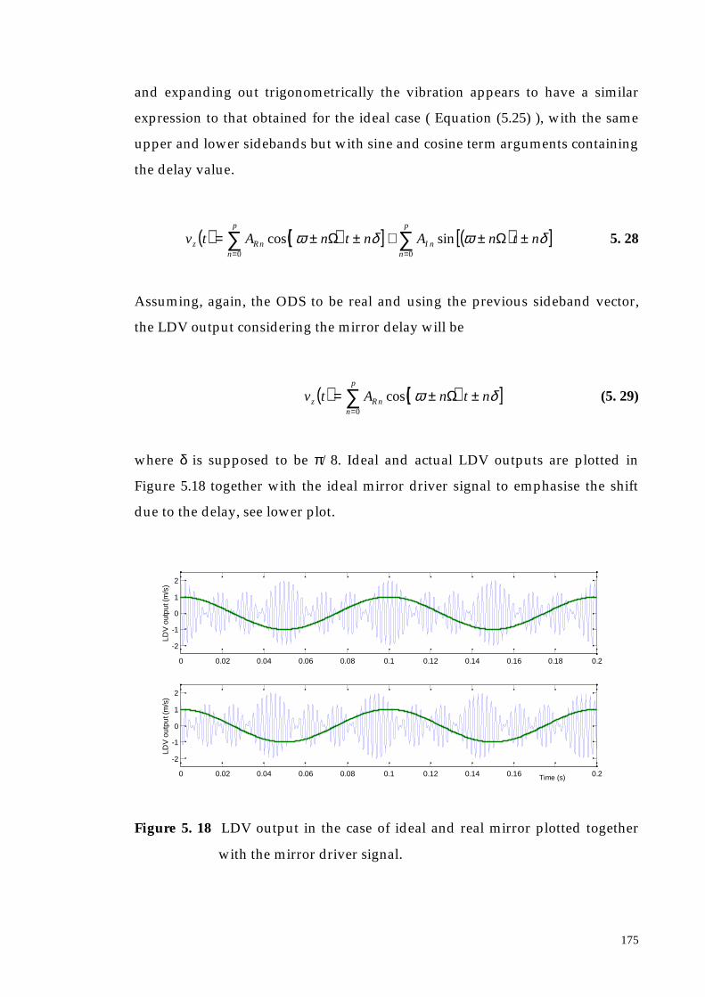
175

and expanding out trigonometrically the vibration appears to have a similar

expression to that obtained for the ideal case ( Equation (5.25) ), with the same

upper and lower sidebands but with sine and cosine term arguments containing

the delay value.

( ) ( )[ ] ( )[ ]∑∑==

±±+±±=p

nnI

p

nnRz ntnAntnAtv

00

sincos δωδω ΩΩ 5. 28

Assuming, again, the ODS to be real and using the previous sideband vector,

the LDV output considering the mirror delay will be

( ) ( )[ ]∑=

±±=p

nnRz ntnAtv

0

cos δω Ω (5. 29)

where δ is supposed to be π/8. Ideal and actual LDV outputs are plotted in

Figure 5.18 together with the ideal mirror driver signal to emphasise the shift

due to the delay, see lower plot.

Figure 5. 18 LDV output in the case of ideal and real mirror plotted together

with the mirror driver signal.

0 0.02 0.04 0.06 0.08 0.1 0.12 0.14 0.16 0.18 0.2

-2

-1

0

1

2

LDV

out

put (

m/s

)

0 0.02 0.04 0.06 0.08 0.1 0.12 0.14 0.16 0.18 0.2

-2

-1

0

1

2

Time (s)

LDV

out

put (

m/s

)

Time (s)

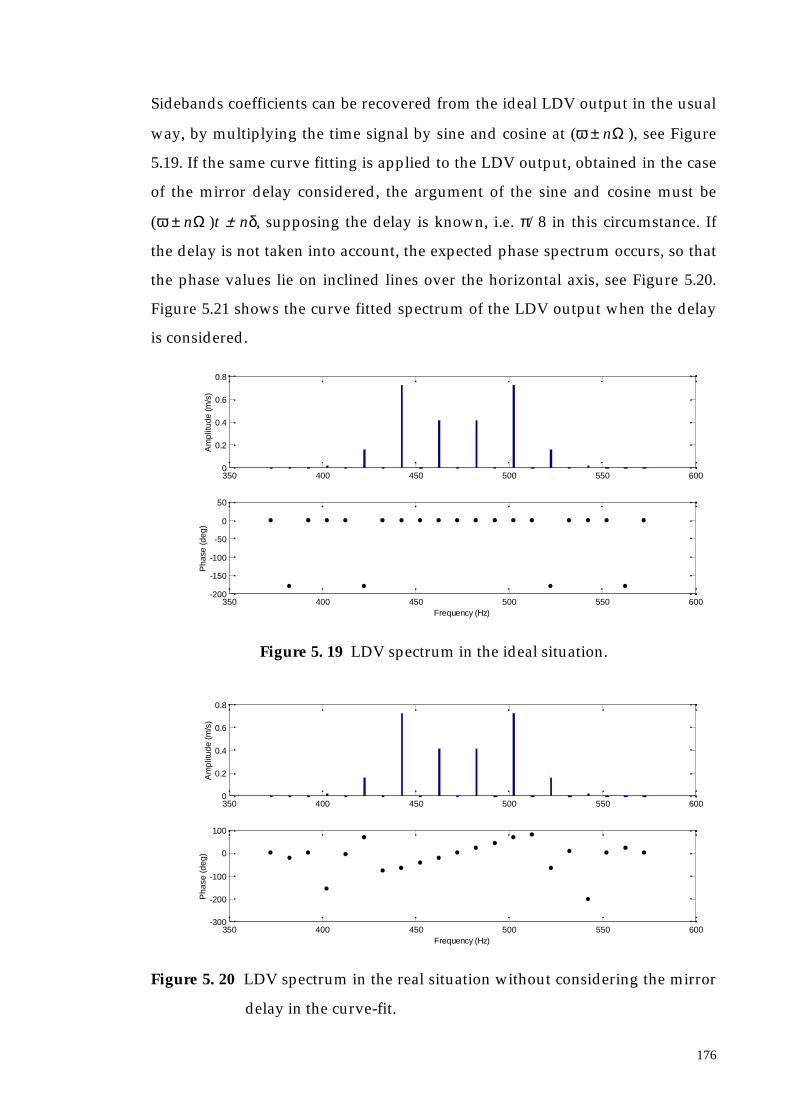
176

Sidebands coefficients can be recovered from the ideal LDV output in the usual

way, by multiplying the time signal by sine and cosine at (ω ± nΩ ), see Figure

5.19. If the same curve fitting is applied to the LDV output, obtained in the case

of the mirror delay considered, the argument of the sine and cosine must be

(ω ± nΩ )t ± nδ, supposing the delay is known, i.e. π/8 in this circumstance. If

the delay is not taken into account, the expected phase spectrum occurs, so that

the phase values lie on inclined lines over the horizontal axis, see Figure 5.20.

Figure 5.21 shows the curve fitted spectrum of the LDV output when the delay

is considered.

350 400 450 500 550 6000

0.2

0.4

0.6

0.8

Am

plitu

de (m

/s)

350 400 450 500 550 600-200

-150

-100

-50

0

50

Frequency (Hz)

Pha

se (d

eg)

Figure 5. 19 LDV spectrum in the ideal situation.

350 400 450 500 550 6000

0.2

0.4

0.6

0.8

Am

plitu

de (m

/s)

350 400 450 500 550 600-300

-200

-100

0

100

Frequency (Hz)

Pha

se (d

eg)

Figure 5. 20 LDV spectrum in the real situation without considering the mirror

delay in the curve-fit.

177

350 400 450 500 550 6000

0.2

0.4

0.6

0.8

Am

plitu

de (m

/s)

350 400 450 500 550 600-200

-150

-100

-50

0

50

Frequency (Hz)

Pha

se (d

eg)

Figure 5. 21 LDV spectrum in the real situation considering the mirror delay in

the curve-fit.


The straight-line scan technique has been applied to the same beam employed

in Subsection 5.3.2 and measurements have again been performed by scanning

on half the length of the beam when it is excited at the experimental natural

frequencies of 58 Hz, 311 Hz and 766 Hz corresponding to the first, third, and

fifth mode respectively.

A similar software to the one produced in LabVIEW for the uniform scan

technique was used to control, acquire and post-process measurement data. The

shaker control and acquisition programs are completely identical to the ones

described in subsection 5.3.2.2 (see Appendix A.1.1 for the control panel of the

LabVIEW program driving the shaker and Appendix A1.3 for the control panel

of the LabVIEW program used for the acquisition). The mirror control routine is

different from the one used for uniform straight-line scans, since the waveform

employed to drive the mirror is a sinewave (see Appendix A.1.5 for the control

panel of the LabVIEW program driving the mirrors). The post-process routine,

to which a Matlab version also exists, performs the curve fit of the LDV output

at the known frequencies. Inputs of this program must be the number of

sidebands required and the mirror delay used to correct the phase spectrum

178

and lined up horizontally phase values. The number of sidebands can be

decided after having a quick look at the spectrum of the LDV output, which is

derived and plotted by the program itself. The mirror delay is defined after

some trials until the phase values are lying horizontally and the spectrum

becomes symmetrical.

First, the beam vibrating at its first mode, 58 Hz, was measured with the LDV

scanning continuously at 10 Hz. The acquisition was triggered with the mirror-

driving signal, when it passed through zero, positively going, see Figure 5.22.

0 0.2 0.4 0.6 0.8 1

-0.2

-0.1

0

0.1

0.2

0.3

Time (s)

Am

plitu

de (V

)

LDV output Mirror Driver Signal

Figure 5. 22 Acquired time signals.

A curve fit was performed at the frequencies (ω ± nΩ ) with n = 0..5 (n can not

be bigger than 5 in order not to go up to negative frequencies. However,

observing the LDV output spectrum during the acquisition it can be noticed

that after the fourth order the sideband amplitudes are negligible). With this

operation the mirror delay is not taken into account and in the LDV spectrum

the phase values misalignment can be seen, see Figure 5.23. On the contrary,

assuming for that delay a value of 1.42 rad, the phase spectrum becomes correct

as shown in Figure 5.24, where phase unwrapping is applied as well.

179

0 10 20 30 40 50 60 70 80 90 100 110 1200

0.05

0.1

0.15

Am

plitu

de (V

)

0 20 40 60 80 100 120-300

-200

-100

0

100

Frequency (Hz)

Pha

se (d

eg)

Figure 5. 23 LDV output spectrum without considering the mirror delay.

0 10 20 30 40 50 60 70 80 90 100 110 1200

0.05

0.1

0.15

Am

plitu

de (V

)

0 20 40 60 80 100 120-300

-200

-100

0

100

Frequency (Hz)

Pha

se (d

eg)

Figure 5. 24 Correct LDV output spectrum.

The sideband spectrum is not perfectly symmetrical and this can be related to

the fact that, in reality, the ODS is not completely real and a complex analysis

must be performed. However, the discrepancy is very small (1.3 %) and the

assumption can be kept. The signed sideband vector will be

A = 0.013410 0.11231 0.019779 - 0.0042793 3.0066 e-4 7.5285 e-5

where it was assumed positive sign if the sideband phases were 0° and negative

if they were -180°.

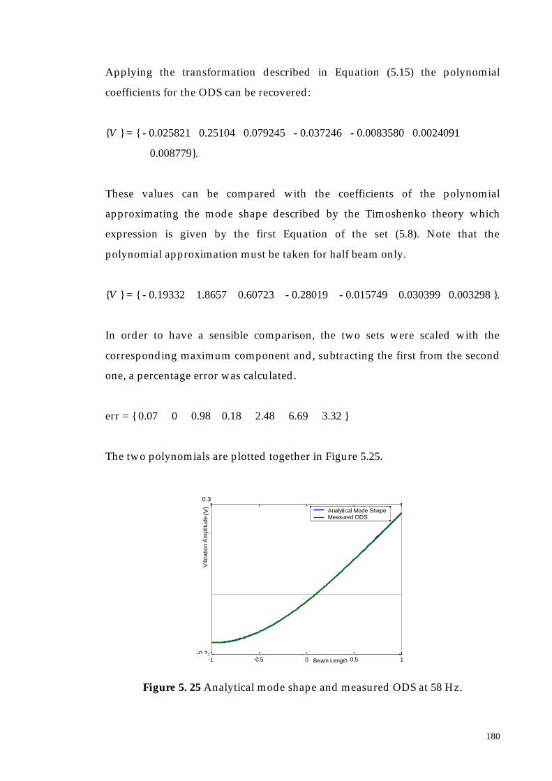
180

Applying the transformation described in Equation (5.15) the polynomial

coefficients for the ODS can be recovered:

V = - 0.025821 0.25104 0.079245 - 0.037246 - 0.0083580 0.0024091

0.008779.

These values can be compared with the coefficients of the polynomial

approximating the mode shape described by the Timoshenko theory which

expression is given by the first Equation of the set (5.8). Note that the

polynomial approximation must be taken for half beam only.

V = - 0.19332 1.8657 0.60723 - 0.28019 - 0.015749 0.030399 0.003298 .

In order to have a sensible comparison, the two sets were scaled with the

corresponding maximum component and, subtracting the first from the second

one, a percentage error was calculated.

err = 0.07 0 0.98 0.18 2.48 6.69 3.32

The two polynomials are plotted together in Figure 5.25.

Figure 5. 25 Analytical mode shape and measured ODS at 58 Hz.

-1 -0.5 0 0.5 1-0.8

Beam Length

Vib

ratio

n A

mpl

itude

Analytical Mode ShapeMeasured ODS

(V)

0.3

-0 2

181

The same procedure can be followed to recover the third and fifth mode shapes:

the ODSs derived by continuous scans and the mode shape simulated by the

Timoshenko theory are plotted together in Figures 5.26 and 5.27 for the natural

frequencies 311 and 766 Hz respectively.



5.3.3.4 Experimental Investigation using the Point-by-Point Technique

Experiments have been carried out in a set of discrete points as well using the

conventional software available from Polytec PSV200. Measurements have been

-1 -0.5 0 0.5 1-0.3

Beam Length

Vib

ratio

n A

mpl

itude Analytical Mode Shape

Measured ODS

0

(V)

-0.2

0.35

-1 -0.5 0 0.5 1Beam Length

Vib

ratio

n A

mpl

itude

Analytical Mode ShapeMeasured ODS

0

(V)

0.4

-0.3

182

performed in the same set-up employed for continuous scanning tests and, in

practice, 47 points, uniformly distributed along the line scan, have been

addressed, see Figure 5.28.

Results are plotted together with the associated ODSs, derived by the CSLDV

technique, in Figures 5.29, 5.30 and 5.31 for the first, third and fifth modes

respectively. Dots in the plot represent the exact position of the laser spot along

the line during the measurement. Resonance frequencies found during the PSV

test were slightly different from the ones observed during the continuous

scanning and their values are reported in Table 5.6.

Figure 5. 28 Single points location.

Single Points Test Continuous Scan Test

FIRST MODE 58.12 Hz 58 Hz

THIRD MODE 312.81 Hz 311 Hz

FIFTH MODE 770.01 Hz 766 Hz

Table 5. 6 Resonance frequencies observed in both the tests performed.

z

x

y

line scan

free-freebeam

singlepoints

183

by CLSDVby SLDV

by CLSDVby SLDV

-1 -0.5 0 0.5 1-2

-1.5

-1

-0.5

0

0.5

1

1.5

2

2.5

3x 10

-4

Half-Beam

Vib

ratio

n V

eloc

ity (m

/s)

Figure 5. 29 ODS corresponding to the first mode.

-1 -0.5 0 0.5 1-3

-2

-1

0

1

2

3x 10

-4

Half-Beam

Vib

ratio

n V

eloc

ity (m

/s)

Figure 5. 30 ODS corresponding to the third mode.

184

by CSLDVby SLDV

-1 -0.5 0 0.5 1-2.5

-2

-1.5

-1

-0.5

0

0.5

1

1.5

2x 10

-4

Half-Beam

Vib

ratio

n V

eloc

ity (m

/s)

Figure 5. 31 ODS corresponding to the fifth mode.

The results clearly correspond closely, but the coarse resolution of the point-by-

point survey is very marked as is the irregularity of the shape.

5.4. Analysis of Circular Scan

5.4.1 Introduction

The continuously-scanning laser Doppler vibrometry can be extended to two-

dimensional structures such as plates of any shape by forcing the laser beam to

move on a trajectory covering the structure surface and following a 2-D path. In

order to realise this, the second mirror in the scanning system of the LDV must

be employed. Driving both mirrors with two sinewaves of different amplitudes,

phases and frequencies, an arbitrarily trajectory can be built to be imposed to

the laser spot, either in Cartesian or polar co-ordinates. However, the easiest 2-

D path that the laser can follow is a large circular scan which covers the greatest

amount of the surface possible, see Figure 5.32. This type of scanning is an

extension of the straight-line scan where the line is now a circle. Moreover, the

velocity of the laser spot following the circle is uniform; specifically, the angular

velocity is Ω, which is the scan speed. The ODS along the circular line can then

be recovered in a straightforward fashion by demodulating the LDV output, as

185

seen in Subsection 5.3.1. Also, if it is possible that the mode shape along the

circular path can be expanded as a spatial Fourier series in the circular

coordinate, then the CSLDV output spectrum will have a known sideband-like

appearance from which the ODS can be directly recovered. This technique can

be applied for measuring out-of-plane vibration of plates, discs or disc-like

components steady or rotating, see references [6], [7] and [18].

Figure 5. 32 Cantilever square plate and disc together with the laser beam

trajectory.

5.4.2 Mathematical Investigation

It is again assumed that the structural vibration or the motion of any point on

the test specimen is approximately sinusoidal at the specific frequency, ω. The

vibration velocity in the z-direction, namely the direction perpendicular to the

vibrating surface, nominally in the plane x,y, is a function of the spatial position

and the time according to the customary relationship:

( ) ( ) ( ) ( ) ( )tsVtsVtsv IRz ωω sincos, += (5. 30)

s, being the circular coordinate around the scan line from a datum position

which is fixed as the start point of the scan. As stated in Section 4.1, if the laser

beam is driven by horizontal and vertical mirrors fed by two sinewaves

of equations Rsin(Ω t) and Rcos(Ω t), respectively, R being the circle radius, the

laser circular

A (start point)

x

y A (start point)

x

y

186

initial point over the circle will be determined by the intersection of the circle

with the y-axis, point A in Figure 5.32. Under this condition, the laser beam

scans uniformly at a rotational speed of Ω. Therefore, the coordinate around the

scan trajectory may be written as ts Ω= , so that, the real and imaginary mode

shape contributions VR and VI , which are functions of the position of the point

on the structure, s, can be expressed in terms of time only. Their spatial

representation can be expanded as Fourier series in the circular coordinate, this

series being upper limited up to, say, the pth terms if the deflection shape is

smooth. It can be then written:

( )

( ) ∑

∑

=

=

=

=

p

nnII

p

nnRR

nsVsV

nsVsV

0

0

sin

cos

(5. 31)

VR n and VI n being the nth spatial Fourier coefficients of the real and imaginary

mode shape components. Substituting the spatial coordinate s with Ωt, the

mode shape contributions can be expressed as functions of time only as the

following equation illustrates:

( ) ( )

( ) ( )∑

∑

=

=

=

=

p

nnII

p

nnRR

tnVtV

tnVtV

0

0

sin

cos

Ω

Ω(5. 32)

At this point, the vibration velocity can be written as:

( ) ( ) ( ) ( ) ( )∑∑==

+=p

nnI

p

nnRz ttnVttnVtv

00

sinsincoscos ωω ΩΩ (5. 33)

The previous equation can be expanded to give:

187

( ) ( ) ( )

( ) ( )[ ] ( ) ( )[ ]∑=

+−−+−+++

++=p

n

nInR

IRz

tnttntV

tnttntV

tVtVtv

1

00

coscos2

coscos2

sincos

ΩΩΩΩ ωωωω

ωω

(5. 34)

where the corresponding terms can be collected to produce:

( ) ( ) ( ) ( ) ( )∑=

+−

+−+

++=p

n

nInRnInRIRz tn

VVtn

VVtVtVtv

100 cos

2cos

2sincos ΩΩ ωωωω

(5. 35)

The vibration velocity then consists of harmonic components at frequencies (ω ±

nΩ) and its spectrum can be seen as a collection of sideband pairs spaced at

± nΩ about the vibration frequency, ω. If the ODS is real, the imaginary

coefficients are all zero (VI n= 0) so that each pair of sideband components have

equal amplitudes. From Equation (5.35) we can conclude that the Fourier

coefficients describing the operating deflection shape of the structure at the

actual excitation frequency can be directly recovered from the spectrum of the

LDV output without passing through the transformation needed in case of

linear scans.

5.4.3 Numerical Simulation on a Rectangular Plate

A circular scan on a rectangular plate, which is illustrated in the first plot of

Figure 5.32, can be simulated by assuming that the vibration pattern along the

scan circle is known and, that it follows the Equation (5.31), i.e. it can be

represented as a Fourier series of the circular coordinate s. Supposing that the

vibration pattern is real only, a set of coefficients VR n can be introduced,

specifically 8, i.e. n = 0...7.

188

Around the circle, the spatial representation of the ODS real component is then

expressed by Equation (5.36) and it is depicted in Figure 5.33.

( ) ( ) ( ) ( ) ( ) ( )( ) ( )ss

ssssssVR

7cos056.06cos031.0

5cos224.04cos562.03cos584.12cos224.0cos100.0778.1

++−+−−+=

(5. 36)

Figure 5. 33 Polynomial ODS along the rectified circle scanned on the plate.

If the laser beam scans in that circle at a speed of 10 Hz, i.e. s = 2π310t , the LDV

will measure a time signal modulated by the mode shape, and it will then be

sensitive to a vibration velocity whose expression is given by Equation (5.33),

adapted to the actual situation:

( ) ( ) ( )[ ] ( )[ ]( )[ ] ( )[ ] ( )[ ]( )[ ] )2112(cos1027cos056.0

1026cos031.01025cos224.01024cos562.0

1023cos584.11022cos224.0102cos100.0778.1

tt

ttt

ttttvz

πππππ

πππ

+++−+

+−−+= (5. 37)

In the previous equation, it was considered that the resonance frequency, ω, of

the actual ODS was 211 Hz. If the LDV signal is acquired using 20000 samples

at a sample rate of 20000 Hz, the time vector t can be introduced in the previous

equation and the time history will appear as Figure 5.34 shows.

VR (s)

s2πππ2

3π2

189

0 0.1 0.2 0.3 0.4 0.5-4

-3

-2

-1

0

1

2

3

4

Time (s)

LDV

out

put

Figure 5. 34 LDV time history modulated by the circumferential mode shape.

By multiplying the LDV time signal by sine and cosine at the well known

frequencies of 2π (211 ± n310) Hz, with n = 0...8, real and imaginary spectral

components are derived, the imaginary ones being negligible since the original

ODS is completely real. The spectral components are illustrated as magnitude

and phase in Figure 5.35.

130 150 170 190 210 230 250 270 2900

0.5

1

1.5

2

Am

plitu

de

140 160 180 200 220 240 260 280 300

0

50

100

150

200

Frequency (Hz)

Pha

se

Figure 5. 35 LDV output spectral components amplitude and phase (°).

On the basis of Equation (5.35), the polynomial coefficients VR n can be recovered

from the sideband amplitudes AR n and sign, following the convention that the

190

sign will be positive if the sideband phase is 0° and negative if it is 180° shifted.

From Figure 5.35 the following sideband vector is derived:

AR = 1.778 0.050 -0.112 -0.792 0.281 -0.112 0.016 0.028

and then it will be V0 = A0 = 1.778 and Vn = 2 An for n = 1..7, therefore:

VR = 1.778 0.100 -0.224 -0.158 0.562 -0.224 0.032 0.056

which are the same as those that appeared in Equation (5.36), which is the

expression describing the ODS over the scan circle. As already mentioned, the

deflection shape along the line scanned can be directly recovered from the LDV

output time history without passing through its Fourier decomposition, by

simply demodulating the time signal itself and filtering out the higher

harmonics, see Subsection 5.3.2. In this case, the scan frequency cannot be too

high as explained above (Subsection 5.3.2); a scan speed of 1 Hz is then

considered. The LDV output will be simulated by Equation (5.37) again with the

only difference being that now the scan frequency is 1 Hz and not 10 Hz. The

time history obtained is shown in Figure 5.36, where a time vector of samples

acquired with a 5000 Hz sample rate is considered.

0 0.2 0.4 0.6 0.8 1-4

-3

-2

-1

0

1

2

3

4

Time (s)

LDV

out

put

Figure 5. 36 LDV output time history zoomed within a scan period (1 sec).

191

By demodulating this signal at the excitation frequency (211 Hz) and applying a

suitable low-pass filter the ODS can be straightforwardly recovered as shown in

Figure 5.37. Note that the picture shows two scan cycles of the laser beam

around the circle, which will take 2 seconds.

0 0.5 1 1.5 2-0.5

0

0.5

1

1.5

2

2.5

3

3.5

4

Time (s)

Vib

ratio

n A

mpl

itude

Figure 5. 37 ODS of the plate around the circle where the laser beam scans.

5.4.4 Numerical Simulation on a Disc

In the context of a vibrating circular disc, VR n and VI n represent spatially

orthogonal, uniform cosine and sine, n-nodal diameter circumferential

amplitude distributions. In fact, provided that the disc is axi-symmetric, its

natural modes occur in pairs, with coincident natural frequencies and nodal

diameters but orthogonal. This results from the solution of the equation

describing the transverse vibration of an axi-symmetric thin disc, which is:

( ) ( ) ( )tnVtnVtv nInRz ωθωθθ sin)sin(cos)cos(, += (5. 38)

vz being the circumferential mode shape including the mode pairs sine and

cosine, and θ the circumferential coordinate.

192

Only when the disc has some slight asymmetry does the so-called mistuning

phenomenon occur and the pairs of orthogonal modes appear at slightly

different natural frequencies. They are then excited to different extents at both

natural frequencies.

In any case, there is always a single value of n and the response mode shape

therefore has n sinewaves around the circumference and 2n equispaced nodes.

In Equation (5.32), the summation will disappear, existing for only a single

value of n and the same will happen for Equation (5.35) implicating that the

CSLDV output spectrum will contain only one pair of sidebands at

frequencies, (ω − nΩ) and (ω + nΩ), Ω being the scan speed of the laser beam

around a circle on the periphery of the disc.

If VI n is zero, so that the response mode shape is completely real and visualised

as a pure standing wave fixed with respect to the disc (see Figure 5.38) the

sideband amplitudes are equal (see the top plot in Figure 5.41).

Figure 5. 38 Standing wave on the disc circumference, case of 3-diameter mode.

If VI n and VR n are equal, the response is a uniform travelling wave (Figure 5.39)

with all points around the circle experiencing the same vibration amplitude,

and there is only one frequency component in the LDV spectrum - at (ω − nΩ),

see the central plot in Figure 5.41.

vz

θ2πππ2

3 π2

193

Figure 5. 39 Travelling wave on the disc circumference, case of 3-diameter

mode.

In Figure 5.40 a three-dimensional view of the travelling wave around the disc

circumference is shown.

Figure 5. 40 2-D view of the travelling wave on the disc circumference.

If VI n and VR n assume different values the disc response will consists of a

travelling and a standing wave. The LDV output spectrum appears, then, with

two sidebands of different magnitudes at (ω − nΩ) and (ω + nΩ) and the

amplitude difference give us an information about the percentage of the

vz

θ2πππ2

3 π2

travelling direction

x

y

ztravelling direction

194

contribution of the travelling wave to the whole complex ODS (see the bottom

plot in Figure 5.41). In the pictures shown in Figure 5.41 it is assumed that the

resonance frequency of the disc is 681 Hz and the ODS is a 3-diameter mode. If

a scan frequency of 10 Hz is employed the sideband frequency are 651 and 711

Hz, when they occur both.

600 650 700 750 8000

2

4

6

Frequency (Hz)

LDV

out

put

spec

trum

Mag

nitu

de

600 650 700 750 8000

2

4

6

Frequency (Hz)

LDV

out

put

spec

trum

Mag

nitu

de

600 650 700 750 8000

2

4

6

8

Frequency (Hz)

LDV

out

put

spec

trum

Mag

nitu

de

TRAVELLINGWAVE PORTION

TRAVELLING WAVE

STANDING WAVE

Figure 5. 41 LDV output spectrum for VI n = 0 (top plot), VI n = VR n (central plot)

and VI n ≠ VR n ≠ 0 (bottom plot).

195

5.4.5 Experimental Investigation on a Disc

The vibration of circular stationary discs has been studied using the circular-

scanning LDV technique working through the same control, data acquisition

and post-process program software developed in LabVIEW for the linear

scanning described in subsection 5.3.2.2 and 5.3.3.3, with slight modifications.

It must be noted that a main source of systematic error, and one which can be

difficult to calibrate out, is scan distortion. Input signal distortion or non-

linearity in the LDV deflection mirror drive system may, in the case of “circular

scan”, produce distortion of the circular scan trace. This can be corrected but,

even after such correction, it is difficult to guarantee that the circle is followed

at precisely uniform rate.

The circular scanning technique was applied on a test piece that was taken from

an application to the problems of disc-brake squeal, specifically a pin-on-disc

rig, where an inclined pin is pressed against a rotating disc. If the pin

arrangement is suitably adjusted, the disc will exhibit limit-cycle parametric

vibration, the so-called ‘squeal’, even at very low speeds of rotation. The

arrangement is simpler than for a vehicle brake disc assembly, there being, for

instance, point contact rather than area contact where the pin and disc are

pressed together. The phenomenon is essentially non-linear, being friction-

induced, but the disc itself generally vibrates in a sinusoidal vibration with an

n-diameter ODS. The disc has then been analysed under the condition of self-

induced vibration due to the squeal excitation but also with discrete frequency

input excitation by removing the pin and producing the input force via a shaker

attached to the structure.

The disc tested was an aluminum 406 mm diameter and 25.4 mm thick uniform

disc around whose circumference the LDV was set up to scan in a circle at 10

Hz rotational speed. In setting up the scanning, particular care must be taken of

the alignment of the scan axis with the disc axis of rotation. In fact, the LDV

measures the velocity of the point addressed, in the direction of the incident

196

measurement beam, which is not exactly perpendicular to the surface, the LDV

being set up on the rotation axis of the disc. Therefore, it actually measures the

vibration resolved onto an inclined line, but, since the angle involved is usually

no more than about 10°, the correction is subsequently quite small. Of more

importance it is the mentioned alignment if the measurement is to be made on a

rotating disc, otherwise the LDV detects a proportion of the rotational velocity,

apparent in the LDV output signal as a component at the LDV scan frequency.

Disc peripheral speeds can be very high compared with the vibration velocities

to be measured and this interference can be overwhelming unless the alignment

is very precise.

First, the disc vibrating only under direct excitation was addressed; the

schematic configuration of the experimental structure is sketched in Figure 5.42.

The disc was excited at some of its resonance frequencies already known from a

previous measurements campaign, and in particular these were chosen at 128,

130.9, 996, 1016, 2307, and 3887.68 Hz. Note that the lower frequencies appear in

pairs and for each couple the same nodal diameter mode was excited. This

means that the disc was slightly mistuned and the natural frequencies of each of

the mode pairs did not coincide exactly. The spectrum amplitude for the above-

listed frequencies are plotted in Figures 5.43, 5.44, 5.45 and 5.46 where in the

first two pictures the coupled frequencies, 128 and 130.9 Hz, 996 and 1016 Hz

are plotted together.

Figure 5. 42 Disc under direct excitation (pin-on-disc rig).

motor driver

shaker

disc shaft

bearing

disc

laser beamscan

x

y

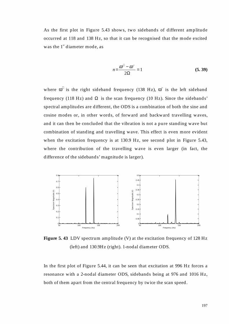
197

As the first plot in Figure 5.43 shows, two sidebands of different amplitude

occurred at 118 and 138 Hz, so that it can be recognised that the mode excited

was the 1st diameter mode, as

12

=−=−+

Ωωω

n (5. 39)

where ω+ is the right sideband frequency (138 Hz), ω− is the left sideband

frequency (118 Hz) and Ω is the scan frequency (10 Hz). Since the sidebands’

spectral amplitudes are different, the ODS is a combination of both the sine and

cosine modes or, in other words, of forward and backward travelling waves,

and it can then be concluded that the vibration is not a pure standing wave but

combination of standing and travelling wave. This effect is even more evident

when the excitation frequency is at 130.9 Hz, see second plot in Figure 5.43,

where the contribution of the travelling wave is even larger (in fact, the

difference of the sidebands’ magnitude is larger).

50 100 150 2000

0.1

0.2

0.3

0.4

0.5

0.6

0.7

0.8

Frequency (Hz)

Spe

ctru

m M

agni

tude

(V

)

50 100 150 2000

0.05

0.1

0.15

0.2

0.25

0.3

0.35

0.4

0.45

0.5

Frequency (Hz)

Spe

ctru

m M

agni

tude

(V

)

Figure 5. 43 LDV spectrum amplitude (V) at the excitation frequency of 128 Hz

(left) and 130.9Hz (right). 1-nodal diameter ODS.

In the first plot of Figure 5.44, it can be seen that excitation at 996 Hz forces a

resonance with a 2-nodal diameter ODS, sidebands being at 976 and 1016 Hz,

both of them apart from the central frequency by twice the scan speed.

198

850 900 950 1000 1050 1100 11500

0.02

0.04

0.06

0.08

0.1

0.12

0.14

0.16

0.18

0.2

Frequency (Hz)

Spe

ctru

m M

agni

tude

(V

)

850 900 950 1000 1050 1100 11500

0.05

0.1

0.15

0.2

0.25

Frequency (Hz)

Spe

ctru

m M

agni

tude

(V

)

Figure 5. 44 LDV spectrum amplitude (V) at the excitation frequency of 996 Hz

(left) and 1016 Hz (right). 2-nodal diameter ODS.

Response sideband peaks at both the excitation frequencies of 996 and 1016 Hz

have identical magnitude so that the corresponding ODSs are seen to be pure

standing waves.

The third and fourth nodal diameter ODSs are excited, finally, at the

frequencies of 2307 Hz and 3887.78 Hz and these are illustrated in Figures 5.45

and 5.46.

2000 2100 2200 2300 2400 2500 26000

0.1

0.2

0.3

0.4

0.5

0.6

0.7

0.8

0.9

1

Frequency (Hz)

Spe

ctru

m M

agni

tude

(V

)

Figure 5. 45 LDV spectrum amplitude (V) at the excitation frequency of 2307

Hz. 3-nodal diameter ODS.

199

3600 3700 3800 3900 4000 4100 42000

0.005

0.01

0.015

0.02

0.025

0.03

0.035

0.04

0.045

Frequency (Hz)

Spe

ctru

m M

agni

tude

(V

)

Figure 5. 46 LDV spectrum amplitude (V) at the excitation frequency of 3887.68

Hz. 4-nodal diameter ODS.

Both the 3rd and 4th nodal diameter ODSs are pure standing waves, the sideband

amplitudes being equal. From the LDV output spectrum shown in Figure 5.46 it

can be noticed that the vibration amplitude at the resonance frequency of

3887.68 Hz was really low and the floor noise assumed more inportance.

The 3rd nodal diameter ODS at frequency of 2307 Hz is recovered following the

mathematical procedure described in this section, strictly speaking Equation

(5.35). From this it can be observed that the vibration velocity measured by the

LDV contains the third component only (n = 3). Then Equation (5.35) can be

written as:

( ) ( ) ( )tVV

tVV

tv IRIRz ΩΩ 3cos

23cos

23333 +

−+−

+= ωω (5. 40)

where 2

33 IR VV + is the spectral amplitude at (ω - 3Ω ) = 2277 Hz and

233 IR VV −

the spectral amplitude at (ω + 3Ω) = 2337 Hz. Knowing the LDV sensitivity

which is 5 mm/s/V the sideband amplitudes readable in Figure 5.45 can be

expressed in terms of velocity:

200

( )

=

×== +− s

mm

V

smmVAA 6433.4

/59286.0)3()3( ΩΩ ωω (5. 41)

Then the polynomial coefficients VR 3 and VI 3 can be recovered from:

=

−

=

+

s

mmVV

s

mmVV

IR

IR

6433.42

6433.42

33

33

(5. 42)

so that,

==

s

mmVV IR 6433.433 (5. 43)

Equation (5.38) then becomes:

( ) )3sin(6433.4)3cos(6433.4 θθθ +=zv (5. 44)

This equation represents the ODS along the circle scanned by the LDV and it is

a pure standing wave, as depicted in Figure 5.47.

Figure 5. 47 Standing wave along the scanning circle (3-nodal diameter ODS).

xy

z

201

In the case of parametric excitation of the pin-on-disc rig (squeal), vibration is

forced at the frequency of 2307 Hz and the involved ODS is then a standing

wave fixed in space. The squeal was produced by pressing the pin against

the disc rotating at 1.9 rpm (0.0317 Hz), see Figure 5.48.

Figure 5. 48 Pin-on-disc rig – “squeal” excitation.

Using again a circular LDV scan at 10 Hz, in the same direction of the disc

rotation, the LDV squeal signal spectrum is acquired and it is virtually identical

with the previous spectrum, for the case of shaker excitation, shown in Figure

5.45. The LDV time signal modulation was seen to be fixed in time relative to

the mirror drive signals, Figure 5.49, with an anti-node at the pin contact

position as Figure 5.50 clearly shows. The disc was therefore rotating slowly

through a standing wave, which was fixed in the non-rotating frame of

reference.

motor driver

disc shaft

bearingdisc

laser beamscan

x

y

pin

disc rotation

202

Figure 5. 49 LDV Time signal and mirror drive signal.

Figure 5.50 3-nodal diameter ODS at 2307 Hz. Standing wave with an antinode

at the pin position.

This technique can be extended to the measurements of vibration of rotating

discs, provided proper account is taken of the relative motion, since the

response frequencies are modified by the disc rotation. In fact, if the disc is

rotating at an angular speed ΩD , assuming that is possible to apply sinusoidal

vibration to it from a fixed point in space (such a kind of excitation can be

realised in operating machines via non-contacting sources as magnetic fields or

xy

z

pinposition

anti-node

0 0.02 0.04 0.06 0.08 0.1 0.12-4

-3

-2

-1

0

1

2

3

4

5

Time (s)

Tim

e H

isto

ries

(V)

LDV Time Signal Mirror Driver Signal

pin position

203

aerodynamic forces), and if the applied excitation is at frequency ω, in the non-

rotating frame of reference, n-diameter ODSs are excited, in the local, rotating

disc coordinates at two distinct frequencies (ω ± nΩD). Equation (5.38), will then

contain four components:

( ) ( )[ ] ( )[ ]( )[ ] ( )[ ]tnnVtnnV

tnnVtnnVtv

DnIDnI

DnRDnRz

ΩΩ

ΩΩ

++−+

+++−=+−

+−

ωθωθ

ωθωθθ

sin)sin(sin)sin(

cos)cos(cos)cos(,(5. 45)

θ being the angular position of a point along the circumference of the disc. If

the LDV laser beam scans around the circumference at an absolute speed ΩL ,

the laser beam angular position relative to the disc at the time instant t will be:

( )tDL ΩΩ −=θ (5. 46)

Substituting Equation (5.46) into (5.45) and expanding trigonometrically it will

become:

( ) ( )( )[ ]

( )[ ]

( )[ ]

( )( )[ ]tnVV

tnVV

tnVV

tnVV

tv

LDnInR

LnInR

LnInR

LDnInR

z

ΩΩ

Ω

Ω

ΩΩ

−+−

+++

+

+−−

+

+−−+

=

++

++

−−

−−

2cos2

cos2

cos2

2cos2

,

ω

ω

ω

ωθ

(5. 47)

As result, there are four frequency components in the SLDV output spectrum

for each diametral order. They appear as sidebands, spaced by multiples of the

laser beam speed relative to the disc, n (ΩL − ΩD), centered on the disc

frequency (ω ± nΩD). From the spectral component values, the unknown

vibration amplitudes, −+−+nInInRnR VVVV ,,, can be easily recovered.

204

In many practical cases, excitation is due to steady forces fixed in a stationary

frame of reference, i.e. ω = 0, so that the disc experiences vibration at frequency

nΩD and responses appear at frequencies nΩL and n (2ΩD − ΩL). With a

symmetrical disc, if nΩD coincides with a natural frequency, a backward

travelling wave will be set up in the disc, or a standing wave in the non-rotating

frame of reference. This is the so-called “critical speed” condition.

5.5. Analysis of Area Scan

5.5.1 Introduction

Out-of-plane vibration response ODS recovery by applying the CSLDV

technique, can be extended to more general two-dimensional scans than the

circular scan described in Section 5.4. Operational mode shapes of a rectangular

or circular area vibrating under a sinusoidal excitation can be conveniently

measured by scanning over the whole area. As for the linear scan, the technique

can be divided into two main branches: a continuous scan at uniform speed,

where the mode shape is directly recovered by demodulation, and a continuous

sinusoidal scan, where the ODS, being approximated by a polynomial, the

relevant series coefficients are derived from the LDV spectral components at the

known discrete frequencies.

The process, involving the demodulation of the LDV output signal can be

applied to any vibrating surface but, since the ODS is directly obtained from the

LDV time history, the data pollution effect of speckle noise may be severe. To

minimise the speckle, the uniform scan speed must, then, kept low. In order to

have enough information from the LDV time history, the acquisition time must

be sufficient for the laser beam to cover all the surface and consequently the

acquisition can become very long. Moreover, a large amount of data may be

generated by using the uniform scanning technique.

Alternatively, the sinusoidal area scan can be employed bearing in mind that its

validity applies only if the mode shape is spatially smooth and without any

205

discontinuities, like, for instance, apertures or sudden changes in section, within

the scanned area. The particular advantage of this technique is that the ODS can

be represented by a smaller data set which consists of the polynomial

coefficients only.

The various test techniques were proven to work in practice with reference to a

simple test piece as the beam was for the linear scan. This consists of a

cantilevered steel plate 172 × 225 × 1 mm thick excited at some of the specific

frequencies where the response was maximum, by a small electro-dynamic

shaker attached off-center to the structure, see Figure 5.51. The plate was the

same as the one used for the test described in Chapter 3 (Section 3.6) but, in this

case it was clamped more deeply and, therefore, the results obtained were

different. In order to validate the continuous-scanning technique the plate was

first tested using the PSV200 software in its conventional mode: a discrete LDV

scan on a grid of points covering the structure surface in reasonable detail. The

plate was excited in a range of frequencies between 0 and 2 kHz, using a

pseudo-random excitation and the laser was scanned step-by-step in a grid of

546 points (see Figure 5.52).

Figure 5. 51 Experimental configuration.

After the measurement acquisition (which took almost three hours) was

completed, the velocity patterns were derived at the resonant frequencies by

SHAKER

PLATE

y

x

CONSTRAINT

206

using the standard PSV200 presentation module. A transfer FRF measured

between the points A and B (excitation position) - shown in Figure 5.52 - is

depicted in Figure 5.53. Only the ODSs at some resonances, corresponding to

the ones analysed by the continuous scanning techniques were taken into

consideration.

Figure 5. 52 Measurement points grid.

0 200 400 600 800 1000 1200 1400 1600 1800 2000-100

-50

0

50

Mag

nitu

de (

dB -

0 dB

= 0

.031

m/s

/N )

0 200 400 600 800 1000 1200 1400 1600 1800 2000-200

-100

0

100

200

Frequency (Hz)

Pha

se (d

eg)

Figure 5. 53 Transfer FRF at point A on the plate.

Resonant frequencies investigated were these at 202.5, 241.25 and 628.8 Hz.

A

B

207

5.5.2 Two-Dimensional Uniform Scan

In making the laser beam scan at a uniform rate, parallel to one side of a

rectangular surface, and simultaneously at a slower uniform rate, parallel to its

other side, the whole area will be covered with a spatial resolution depending

on the data acquisition sampling rate and the two scan rates. In fact, if the

slowest scan frequency is, say, 0.01 Hz, the laser beam will perform a complete

scan in 50 seconds (one pass over the line scanned) and the acquisition of the

LDV output signal must last at least 50 seconds. Since the acquisition time is

determined by the ratio between the number of samples acquired and the

acquisition sampling rate, the number of samples, namely the ODS spatial

resolution, will be 50 times the sample rate. The slower the scan rate, the larger

is the spatial resolution, but the acquisition becomes more time consuming.

Demodulating the LDV time history a two-dimensional ODS is derived with

the spatial position being the time axis. If the demodulated signal is then

plotted against the mirrors’ drive signals, recorded simultaneously with the

LDV output, since they represent the laser spot spatial position over the surface

at each time instant, a three-dimensional surface representing the ODS can be

visualised.

The procedure followed for demodulation is the same as that described in

Subsection 5.3.2 ( Equation (5.7) ) for a one-dimensional scan, the only

difference with the latter is the presentation of results, since the demodulated

signal is now plotted against two spatial position vectors defined by the mirrors

drive time signals.

As an example, the cantilever plate depicted in Figure 5.51 was analysed under

a sinusoidal excitation at 628.8 Hz. Mirrors, driving the laser beam to scan over

the surface of the plate, were fed via two triangular waves in order to force the

laser spot to sweep the x-axis at a uniform rate of 0.12 Hz and the y-axis at 7 Hz.

The pattern followed by the laser beam across the plate’s surface is visualised in

Figure 5.54.

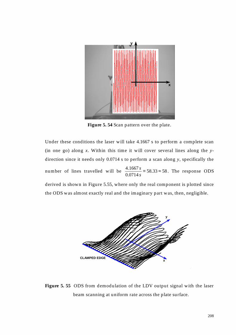
208

Figure 5. 54 Scan pattern over the plate.

Under these conditions the laser will take 4.1667 s to perform a complete scan

(in one go) along x. Within this time it will cover several lines along the y-

direction since it needs only 0.0714 s to perform a scan along y, specifically the

number of lines travelled will be 5833.580714.0

1667.4 ≈=s

s. The response ODS

derived is shown in Figure 5.55, where only the real component is plotted since

the ODS was almost exactly real and the imaginary part was, then, negligible.

Figure 5. 55 ODS from demodulation of the LDV output signal with the laser

beam scanning at uniform rate across the plate surface.

CLAMPED EDGEx

y

x

y

209

5.5.3 Sinusoidal Parallel Straight-Line Scans

The sinusoidal scanning technique can also be applied to area scans, where the

easiest way to do it is to make the laser beam to scan on a set of parallel lines

along which polynomial mode shapes can be defined. The method

straightforwardly applies the sinusoidal straight-line scanning technique

(Subsection 5.3.3 and Equation (5.15) ), the line scanned being parallel to the y-

axis but, in addition, this technique is repeated for several parallel lines evenly

spaced in the x-direction in order to cover all area of the specimen under test.

Plotting in the same diagram the polynomial ODS recovered along each of these

lines, a two-dimensional picture representing the global ODS of the structure is

obtained.

As an example, the usual plate, vibrating at the same excitation frequency of

628.8 Hz, was studied and twenty straight-lines parallel to the y-axis were

scanned at a rate of 10 Hz on its surface. From each scan the LDV time signals

were acquired and curve fitted at the set of frequencies given by (ω ± nΩ) with n

= 0...p and p the polynomial order. From the spectral amplitudes at these

frequencies (An), applying Equation (5.15), the polynomial coefficients (Vn) were

derived and, plotting the ODSs together in a same diagram, Figure 5.56 was

obtained. Again only one plot is shown, the ODS being almost exactly real.

Figure 5. 56 Polynomial ODSs recovered from the LDV output signal in the

frequency domain with the laser beam scanning sinusoidally

along a set of parallel straight-lines covering the plate surface.

CLAMPED EDGEx

y

210

For example, when the first line was scanned the LDV output spectral

amplitudes at (628.8 ± n 10), where n = 0...6 , transformed by the matrix [T] gave

a set of coefficients series which could be written as the following 6th order

polynomial expression:

( ) 55432 5248.43760.00128.101782.15628.67827.29254.0 yyyyyyyv ++−−++=(5. 48)

A similar expression can be derived for each LDV output acquired.

5.5.4 Two-Dimensional Sinusoidal Scans


From the parallel straight lines technique, it can be concluded that, instead of

plot a different set of one-dimensional polynomial series together, which

requires one to perform a number of measurements corresponding to the

number of line scans realised, a two-dimensional polynomial can be obtained

directly in one measurement.

In order to perform an area scan, the laser beam of an LDV must scan at

frequency of Ωx in x-direction and a frequency of Ωy in y-direction. If these two

frequencies are not fractionally related - and they must be so, as it will be

explained later - the scan describes an open Lissajou figure over the scanned

area which can be completely covered after a conveniently short time period. In

order to sweep a normalised area of dimensions 2 × 2, with the zero position the

center of the square, the mirror drivers should be fed by two sinewaves of

equations:

211

( ) ( )( ) ( )tty

ttx

y

x

ΩΩ

cos

cos

==

(5. 49)

The complex amplitudes of the ODS appearing in Equation (5.1) can be written

as two-dimensional polynomial series:

( )

( ) ∑

∑

=

=

=

=

qp

mn

mnmnII

qp

mn

mnmnRR

yxVyxV

yxVyxV

,

0,,

,

0,,

,

,

(5. 50)

p and q being the polynomial order in x- and y-direction respectively.

The vibration velocity, following the principle of Equation (5.1), translated to a

two-dimensional structure, becomes:

( ) ( ) ( ) ( ) ( )tyxVtyxVtyxv IRz ωω sin,cos,;, += (5. 51)

Substituting Equation (5.49) in (5.50) and again in (5.51), Equation (5.51) itself

can be rewritten as:

( ) ( ) ( ) ( ) ( ) ( ) ( )∑∑==

+=qp

mny

mx

nmnI

qp

mny

mx

nmnRz tttVtttVtv

,

0,,

,

0,, sincoscoscoscoscos ωω ΩΩΩΩ

(5. 52)

Expanding out trigonometrically, as was done for the linear scan mathematics

in Subsection 5.3.3.1, the following representation of the vibration signal is

derived:

( ) ( )[ ] ( )[ ]∑∑==

±±+±±=qp

mnyxmnI

qp

mnyxmnRz tmnAtmnAtv

,

0,,

,

0,, sincos ΩΩΩΩ ωω (5. 53)

212

It can be deduced that the transformation to recover the polynomial coefficients

from the spectral amplitudes of the LDV output is:

[ ] [ ] [ ] [ ] T

II

TRR

TATV

TATV

=

=(5. 54)

The previous equation can be demonstrated by expanding, again, the

relationship (5.52), considering n = 0...3 and m = 0...3.

( )

( )[ ]

( )[ ] ( )

( )[ ] ( )[ ]

( )[ ]

( )[ ]

( )[ ] ( )[ ]

( )[ ] ( )[ ]

( )[ ] ( )

( )[ ] ( )[ ]

( )[ ] ( )[ ]

( )[ ] ( )

( )[ ] ( )[ ]

( )[ ] ( )[ ]

( )[ ] ( )[ ]

( )[ ] ( )[ ]tVt

Vmandnfor

tV

tV

mandnfor

tV

tV

tV

tV

mandnfor

tV

tV

tV

tV

mandnfor

tV

tV

mandnfor

tV

tV

mandnfor

tV

tV

mandnfor

tV

tV

mandnfor

tV

mandnfor

tV

mandnfor

tV

tV

mandnfor

tV

tV

mandnfor

tV

mandnfor

tVmandnfor

yxR

yxR

xR

xR

yR

yR

yxR

yxR

Ry

R

xR

yxR

yR

yxR

Rx

R

yxR

yxR

xR

yxR

yxR

xR

yR

yR

Ry

R

yR

R

ΩΩΩΩ

ΩΩ

ΩΩ

ΩΩΩΩ

Ω

ΩΩΩ

ΩΩΩ

Ω

ΩΩΩΩ

ΩΩΩ

ΩΩ

Ω

ΩΩ

Ω

Ω

±±+±±==

±+±==

±+±+

+±±+±±==

+±+

+±+±±==

±+±±==

+±==

±±+±±==

±+±±==

±±==

±==

±+±==

+±==

±==

==

ωω

ωω

ωω

ωω

ωω

ωω

ωω

ωω

ωω

ωω

ω

ω

ωω

ωω

ω

ω

cos16

33cos

1613

cos8

33cos

803

cos16

33cos

16

2cos32

332cos

3232

cos4

2cos8

2cos8

22cos16

22

cos4

2cos8

12

cos2

2cos4

02

cos16

33cos

1631

cos4

2cos8

21

cos4

11

cos2

01

cos8

33cos

830

cos2

2cos4

20

cos2

10

cos00

3131

3030

2323

2323

2222

2222

2121

2020

1313

1212

11

10

0303

0202

01

00

213

( )[ ] ( )[ ]

( )[ ] ( )[ ]

( )[ ] ( )[ ]

( )[ ] ( )[ ]tVt

V

tV

tV

mandnfor

tV

tV

tV

tV

mandnfor

yxR

yxR

yxR

yxR

xR

yxR

xR

yxR

ΩΩΩΩ

ΩΩΩΩ

ΩΩΩ

ΩΩΩ

±±+±±

+±±+±±==

±+±±

+±+±±==

ωω

ωω

ωω

ωω

cos64

93cos

64

3

3cos64

333cos

6433

cos16

32cos

32

3

3cos16

23cos32

23

3333

3333

3232

3232

The LDV output spectrum will then have components at the frequencies

(ω ± nΩx ± mΩy) with the following amplitudes, called Anm:

1683

3232

1622

32

3

82

842

64

3

163

32

3

82

64

9

16

3

16

3

4

16

3

8

3

22

1683

842

16

3

48

3

2

422

323030

2323

2222

232121

222020

331313

321212

3331131111

3230121010

230303

220202

2321030101

2220020000

RRRx

RRyx

RRyx

RRRyx

RRRx

RRRyx

RRRyx

RRRRRyx

RRRRRx

RRRy

RRRy

RRRRRy

RRRRR

VVAat

VAat

VAat

VVAat

VVAat

atVV

Aat

VVAat

VVVVAat

VVVVAat

VVAat

VVAat

VVVVAat

VVVVAat

+=±

=±±

=±±

+=±±

+=±

+=±±

+=±±

+++=±±

+++=±

+=±

+=±

+++=±

+++=

Ω

ΩΩ

ΩΩ

ΩΩ

Ω

ΩΩ

ΩΩ

ΩΩ

Ω

Ω

Ω

Ω

ω

ω

ω

ω

ω

ω

ω

ω

ω

ω

ω

ω

ω

214

6433

3223

64

3

163

3333

3232

333131

RRyx

RRyx

RRRyx

VAat

VAat

VVAat

=±±

=±±

+=±±

ΩΩ

ΩΩ

ΩΩ

ω

ω

ω

which can be written as

=

8108

30

04102

1

00210

0001

81000

04100

8302

10

02101

33323130

23222120

13121110

03020100

33323130

23222120

13121110

03020100

VVVV

VVVV

VVVV

VVVV

AAAA

AAAA

AAAA

AAAA

The polynomial coefficients matrix can then be derived:

−−

−

−

=

8060

0402

0020

0001

8000

0400

6020

0201

33323130

23222120

13121110

03020100

33323130

23222120

13121110

03020100

AAAA

AAAA

AAAA

AAAA

VVVV

VVVV

VVVV

VVVV

where the first numeric matrix appearing, in the left-hand-side of the algebraic

equation, is a truncation of the transform matrix [T] ( see Equation (5.16) ) and

the second matrix is its transpose.


5.5.4.2.1 Real Vibration Response

In order to predict how the output time signal of an LDV will appear when it

scans over the surface of a plate vibrating at one of its natural frequencies, a

simulation of this situation will be performed. First, analytical mode shapes of

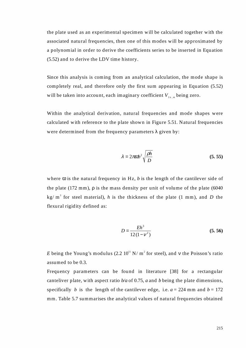
215

the plate used as an experimental specimen will be calculated together with the

associated natural frequencies, then one of this modes will be approximated by

a polynomial in order to derive the coefficients series to be inserted in Equation

(5.52) and to derive the LDV time history.

Since this analysis is coming from an analytical calculation, the mode shape is

completely real, and therefore only the first sum appearing in Equation (5.52)

will be taken into account, each imaginary coefficient VI n , m being zero.

Within the analytical derivation, natural frequencies and mode shapes were

calculated with reference to the plate shown in Figure 5.51. Natural frequencies

were determined from the frequency parameters λ given by:

D

hb

ρπωλ 22= (5. 55)

where ω is the natural frequency in Hz, b is the length of the cantilever side of

the plate (172 mm), ρ is the mass density per unit of volume of the plate (6040

kg/m3 for steel material), h is the thickness of the plate (1 mm), and D the

flexural rigidity defined as:

)1(12 2

3

ν−= Eh

D (5. 56)

E being the Young’s modulus (2.2 1011 N/m2 for steel), and ν the Poisson’s ratio

assumed to be 0.3.

Frequency parameters can be found in literature [38] for a rectangular

canteliver plate, with aspect ratio b/a of 0.75, a and b being the plate dimensions,

specifically b is the length of the cantilever edge, i.e. a = 224 mm and b = 172

mm. Table 5.7 summarises the analytical values of natural frequencies obtained

216

from the frequency parameters taken from references which are also illustrated

in this table.

MODE Reference FrequencyParameter λ

NaturalFrequency

ω (Hz)1 Table 4.51 – symmetric mode 1.946 19.212 Table 4.52 – antisymmetric mode 5.99 58.853 Table 4.51 – symmetric mode 12.09 118.794 Table 4.52 – antisymmetric mode 20.6 202.405 Table 4.51 – symmetric mode 24.7 242.68

Table 5. 7 Analytical values of natural frequencies.

The mode shapes equation is given in literature, [38]:

( )

−−−×

×

+−++

−+= ∑ ∑

= =

a

x

a

x

a

x

a

x

b

y

b

y

b

y

b

yA

a

yAAyxw

mmm

mm

p

m

q

n

nnn

nnmnmm

εεαεε

εεαεε

sinsinhcoscosh

sinsinhcoscosh213,1 3

21

(5. 57)

where the values of Amn and those of α and ε are given in literature as well. The

fourth anti-symmetric mode shape (at a frequency of 202.4 Hz) is then

calculated and its plot is shown in Figure 5.57.

217

Figure 5. 57 Analytical mode shape at the natural frequency of 202.4 Hz.

In order to apply Equation (5.52), the mode shape is approximated by a two-

dimensional polynomial of, say, the 6th order in both the dimensions:

( ) ∑=

=6,6

0,,,

mn

mnmn yxVyxV (5. 58)

with the coefficients matrix:

−−−−−

−−−−−−−−

−−−−−−−

−−−−−

=

0177.00494.00295.01416.00136.04957.00013.0

0028.00581.00047.02376.00022.08637.00

0232.03147.00387.07667.00181.04327.30029.0

0030.00198.00058.07135.00038.05146.00078.0

0051.07443.00086.09595.10043.06566.70141.0

02975.00005.06186.00007.09297.10568.0

0003.01436.00005.02360.00002.04478.20332.0

nmV

(5. 59)

Considering now a laser beam scanning in the x-direction at 1.1 Hz and at 20

Hz in the y-direction, the x and y position can be related to the time so that:

y

y

CANTILEVER EDGE

218

( ) ( )( ) ( )tty

ttx

202cos

1.12cos

ππ

==

(5. 60)

and the LDV will measure a time-dependent velocity signal of the following

form:

( ) ( ) ( ) ( )∑=

=6,6

0,, 4.2022cos202cos1.12cos

mn

mnmnz tttVtv πππ (5. 61)

the natural frequency associated with the mode shape being 202.4 Hz.

The time history to be measured by the LDV is shown in Figure 5.58, assuming

that the acquisition is performed at 20000 samples with a sampling rate of 2000

Hz. Figure 5.59 illustrates the pattern followed by the laser beam on the plate, if

its position is driven by Equation (5.60).

Figure 5. 58 Simulated time histories of the velocity response, together with the

time-dependent position of the laser beam on the plate.

0 0.5 1 1.5-4

-3

-2

-1

0

1

2

3

4

Time (s)

Am

plitu

de

LDV x-mirrory-mirror

(V)

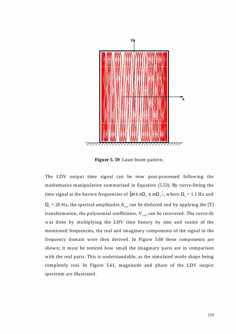
219

Figure 5. 59 Laser beam pattern.

The LDV output time signal can be now post-processed following the

mathematics manipulation summarised in Equation (5.53). By curve-fitting the

time signal at the known frequencies of ( )yx mn ΩΩ ±±ω , where Ωx = 1.1 Hz and

Ωy = 20 Hz, the spectral amplitudes An,m can be deduced and by applying the [T]

transformation, the polynomial coefficients, Vn,m, can be recovered. The curve-fit

was done by multiplying the LDV time history by sine and cosine of the

mentioned frequencies, the real and imaginary components of the signal in the

frequency domain were then derived. In Figure 5.60 these components are

shown; it must be noticed how small the imaginary parts are in comparison

with the real parts. This is understandable, as the simulated mode shape being

completely real. In Figure 5.61, magnitude and phase of the LDV output

spectrum are illustrated.

x

y

220

50 100 150 200 250 300 350-0.2

0

0.2

0.4

0.6

Rea

l Com

pone

nts

50 100 150 200 250 300 350-2

0

2

4

6

8x 10

-13

Frequency (Hz)

Imag

inar

y C

ompo

nent

s

Figure 5. 60 Real and imaginary components (in V) of the LDV output

spectrum.

50 100 150 200 250 300 3500

0.1

0.2

0.3

0.4

0.5

Mag

nitu

de

50 100 150 200 250 300 350-200

-150

-100

-50

0

50

Frequency (Hz)

Pha

se (d

eg)

Figure 5. 61 Magnitude (in V) and phase of the LDV output spectrum.

The sideband matrix An,m, which is unique in this case, since the mode is real,

can be derived from the magnitude of the LDV output spectrum and its sign

from the phase. This matrix is associated with the spectral components as is

explained in the diagram of Figure 5.62. If

221

=

nmnnn

m

m

m

mn

AAAA

AAAA

AAAA

AAAA

A

..

......

......

..

..

..

.

210

2222120

1121110

0020100

,

the spectral components can then be named as in Figure 5.62.

Figure 5. 62 Association between the LDV spectral amplitudes and the

sideband matrix components.

As has been demonstrated mathematically, in the case of purely real mode

shapes, the symmetrical sideband components have identical amplitudes so the

sideband matrix can then be composed of only one component of each

sideband’s pair. The x-sidebands group (A00, A01, A02 ..., and A10, A11, A12 ...) will be

the columns of the sidebands matrix, while the y-sidebands group (A00, A10, A20

..., and A01, A11, A21 ...) will be the rows of this matrix.

Each matrix element can be associated with a positive or negative sign by

observing the spectral phase of the LDV output. In fact, all the spectral

components are in phase with each other or they have a shift of 180°. Referring

all the component’s phase to that of the central component, it can be

A00

A01 A10

A12

A13

A14

A15...

A11A1-1

A1-2

A1-3

A1-4

A1-5

A02

A03

A04

A05...

A0-1

A0-2

A0-3

A0-4

A0-5

A -10

A -11

A -12

A -13

A -14

A –15...

A -1-1

A –1 -2

A –1-3

A –1-4

A –1-5

Frequency

x-sidebands groupsidebands spaced of thescan frequency on x-direction

y-sidebands groupsidebands spaced of the scanfrequency on y-direction

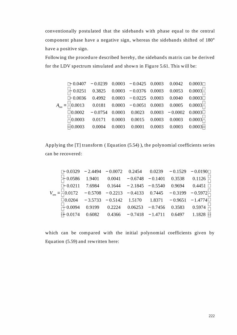
222

conventionally postulated that the sidebands with phase equal to the central

component phase have a negative sign, whereas the sidebands shifted of 180°

have a positive sign.

Following the procedure described hereby, the sidebands matrix can be derived

for the LDV spectrum simulated and shown in Figure 5.61. This will be:

−−−−−−−−−−

=

0003.00003.00003.00001.00003.00004.00003.0

0003.00003.00003.00015.00003.00171.00003.0

0003.00002.00003.00023.00003.00754.00002.0

0003.00005.00003.00051.00003.00181.00013.0

0003.00040.00003.00225.00003.04992.00036.0

0003.00053.00003.00376.00003.03825.00251.0

0003.00042.00003.00425.00003.00239.00407.0

nmA

Applying the [T] transform ( Equation (5.54) ), the polynomial coefficients series

can be recovered:

−−−−−

−−−−−−−−−

−−−−−−

−−−−−

=

1828.16497.04711.17418.04366.06082.00174.0

5974.03583.07456.006253.02224.09199.00094.0

4774.19651.08371.15170.15142.05733.30204.0

5972.03199.07445.04133.02213.05708.00172.0

4451.09694.05540.01845.21644.06984.70211.0

1126.03538.01401.06748.00041.09401.10586.0

0190.01529.00239.02454.00072.04494.20329.0

nmV

which can be compared with the initial polynomial coefficients given by

Equation (5.59) and rewritten here:

223

−−−−−

−−−−−−−−

−−−−−−−

−−−−−

=

0177.00494.00295.01416.00136.04957.00013.0

0028.00581.00047.02376.00022.08637.00

0232.03147.00387.07667.00181.04327.30029.0

0030.00198.00058.07135.00038.05146.00078.0

0051.07443.00086.09595.10043.06566.70141.0

02975.00005.06186.00007.09297.10568.0

0003.01436.00005.02360.00002.04478.20332.0

, INITIALnmV

The derived polynomial coefficients, Vn,m, can be used to recover the ODS

already shown in Figure 5.57.

5.5.4.2.2 Complex Vibration Response

A more general case, where the simulated mode shape is complex, is addressed

next. It is assumed that the real and imaginary components of the mode shape,

again at 202.4 Hz (ω), are equal and they can be approximated by the same

polynomial and the polynomial coefficients series VRnm and VInm are the same

(Equation (5.59) ). Both the two addenda of Equation (5.52) must be considered

in this case and they will produce an LDV output vz(t) whose spectrum is, now

complex, i.e. real and imaginary components are comparable (Figure 5.63).

50 100 150 200 250 300 350-0.2

0

0.2

0.4

0.6

Rea

l Com

pone

nts

50 100 150 200 250 300 350-0.6

-0.4

-0.2

0

0.2

Frequnecy (Hz)

Imag

inar

y C

ompo

nent

s

Figure 5. 63 Real and imaginary components of the LDV output spectrum.

224

Observing the LDV output spectrum in amplitude and phase (Figure 5.64), it is

possible to notice that all the points are no longer in phase with each other, or

180° phase-shifted. This is because the ODS measured is complex and the

spatial points are not in phase with each other as well.

50 100 150 200 250 300 3500

0.2

0.4

0.6

0.8

Mag

nitu

de

50 100 150 200 250 300 350-400

-300

-200

-100

0

100

Frequency (Hz)

Pha

se (d

eg)

Figure 5. 64 Magnitude and phase of the LDV output spectrum.

From the real and imaginary components of the LDV spectrum the sidebands

matrix ARnm and AInm can be derived. The procedure to recover their sign is not

necessary anymore because the real and imaginary components are now

comprehensive of the sign.

−−−−−−−−−−

=

0003.00003.00003.00001.00003.00035.00003.0

0003.00003.00003.00015.00003.00171.00003.0

0003.00002.00003.00023.00003.00754.00002.0

0003.00005.00003.00051.00003.00181.00013.0

0003.00040.00003.00225.00003.04992.00036.0

0003.00053.00003.00376.00003.03825.00251.0

0003.00042.00003.00425.00003.00239.00407.0

RnmA

225

−−−−

−−−−−−−−

=

0000001.000033.00

0000012.000168.00

00004.000019.000757.00

00002.000054.000178.00009.0

00037.000228.004989.00039.0

00049.000379.003822.00255.0

00039.000428.000242.00409.0

InmA

From the sidebands matrices the 2-D polynomial coefficients series are derived

applying the transform in Equation (5.54):

−−−−−

−−−−−−−−−

−−−−−−

−−−−−

=

1828.16497.04711.17418.04366.06082.00174.0

5974.03583.07456.006253.02224.09199.00094.0

4774.10651.18371.15170.15142.05733.30204.0

5972.03199.07445.04133.02213.05708.00172.0

4451.09694.05540.01845.21644.06984.70211.0

1126.03538.01401.06748.00041.09401.10586.0

0190.01529.00239.02454.00072.04494.20329.0

RnmV

−−−−−−−−

−−−−−−

−−−−−−

−−

=

0178.00494.00295.01416.00013.04956.00013.0

0028.00581.00047.02376.00026.08637.00

0232.03147.00387.07134.00181.04326.30029.0

0030.00198.00058.07134.00038.05145.00078.0

0051.07443.00087.09594.10043.06562.70141.0

02975.00005.06185.00007.0929.10568.0

0003.01435.00005.02361.00002.04477.20332.0

InmV

Real and imaginary components of the ODS given by the previous polynomial

coefficients series are shown in Figures 5.65 and 5.66 respectively.

226

Figure 5. 65 Real components of the recovered ODS.

Figure 5. 66 Imaginary components of the recovered ODS.

5.5.4.2.3 Mirror Delay Effect

A further detail which must taken into account is the mirror delay already

discussed in Chapter 4 (Section 4.6). In practice, the sinewaves followed by the

laser beam over the plate surface are never completely equal to the ones driving

the mirrors and given by Equation (5.49). Usually, the laser beam presents a

x

y

CANTILEVER EDGE

x

y

227

slight delay, which can be called δx in x-direction and δy in y-direction. The laser

beam will then travel according to the following relationship:

( ) ( )( ) ( )yy

xx

tty

ttx

δδ

+=+=

ΩΩ

cos

cos(5. 62)

Equation (5.52) will become:

( ) ( ) ( ) ( )

( ) ( ) ( )∑

∑

=

=

+++

+++=

qp

mnyy

mxx

nmnI

qp

mnyy

mxx

nmnRz

tttV

tttVtv

,

0,,

,

0,,

sincoscos

coscoscos

ωδδ

ωδδ

ΩΩ

ΩΩ(5. 63)

In terms of sideband components this can be written ( similarly to Equation

(5.53) ):

( ) ( ) ( )[ ]

( ) ( )[ ]∑

∑

=

=

+±+±+

++±+±=

qp

mnyyxxmnI

qp

mnyyxxmnRz

tmtntA

tmtntAtv

,

0,,

,

0,,

sin

cos

δδω

δδω

ΩΩ

ΩΩ(5. 64)

which leads to:

( ) ( )[ ]

( )[ ]∑

∑

=

=

±±±±+

+±±±±=

qp

mnyxyxmnI

qp

mnyxyxmnRz

mntmnA

mntmnAtv

,

0,,

,

0,,

sin

cos

δδω

δδω

ΩΩ

ΩΩ(5. 65)

This means that the mirror delay must be taken into consideration with the

curve-fit process in order to determine the real value of the sideband matrices

components ARnm and AInm to which Equation (5.54) can be applied without any

228

correction. In practical examples the last formulae derived will in any case be

employed and the mirror delay always considered.

Such a situation can be simulated considering an x-mirror delay (δx) of π/8 rad

and a y-mirror delay (δy) of π/10 rad. The LDV time history recovered for a

purely real mode shape approximated by a polynomial with coefficients given

by Equation (5.59) is shown in Figure 5.67, where the upper plot represents the

time signal derived without any delay and using Equation (5.52), while the

lower plot represents the LDV output in the real situation derived applying

Equation (5.63). It can be noticed that the LDV time history is not in phase with

the sinewaves (red and green) which are the signal driving the mirrors (not

affected by the delay, since they are the signals drivers upstream of the inertia

of the mirrors).

0 0.2 0.4 0.6 0.8 1 1.2 1.4 1.6 1.8-4

-2

0

2

4

LDV

out

put (

m/s

)

0 0.2 0.4 0.6 0.8 1 1.2 1.4 1.6 1.8-4

-2

0

2

4

Time (s)

LDV

out

put (

m/s

)

Figure 5. 67 LDV output signal for the ideal and real situation, considering the

delay of the mirrors, which are plotted as well (the x-mirror is

green and the y-mirror is red).

By performing a curve-fit to the ideal time signal multiplying by sine and

cosine of (ω ± nΩx ± mΩy), the LDV spectrum will appear as shown in Figure

5.68; in contrast, if the time signal is the real one (i.e. the laser beam pattern is

actually delayed) without taking into account the mirrors delay, a phase

spectrum which is completely spread is recovered, see Figure 5.69. On the other

229

hand the spectrum is brought back to the ideal situation if the multiplication is

done by sine and cosine of [(ω ± nΩx ± mΩy )t ± nδx ± mδy], see Figure 5.70.

50 100 150 200 250 300 3500

0.1

0.2

0.3

0.4

0.5M

agni

tude

50 100 150 200 250 300 350-200

-150

-100

-50

0

50

Frequency (Hz)

Pha

se (d

eg)

Figure 5. 68 LDV spectrum in the ideal situation.

50 100 150 200 250 300 3500

0.1

0.2

0.3

0.4

0.5

Mag

nitu

de

50 100 150 200 250 300 350-300

-200

-100

0

100

Frequency (Hz)

Pha

se (d

eg)

Figure 5. 69 LDV spectrum in the real situation without considering the mirror

delay.

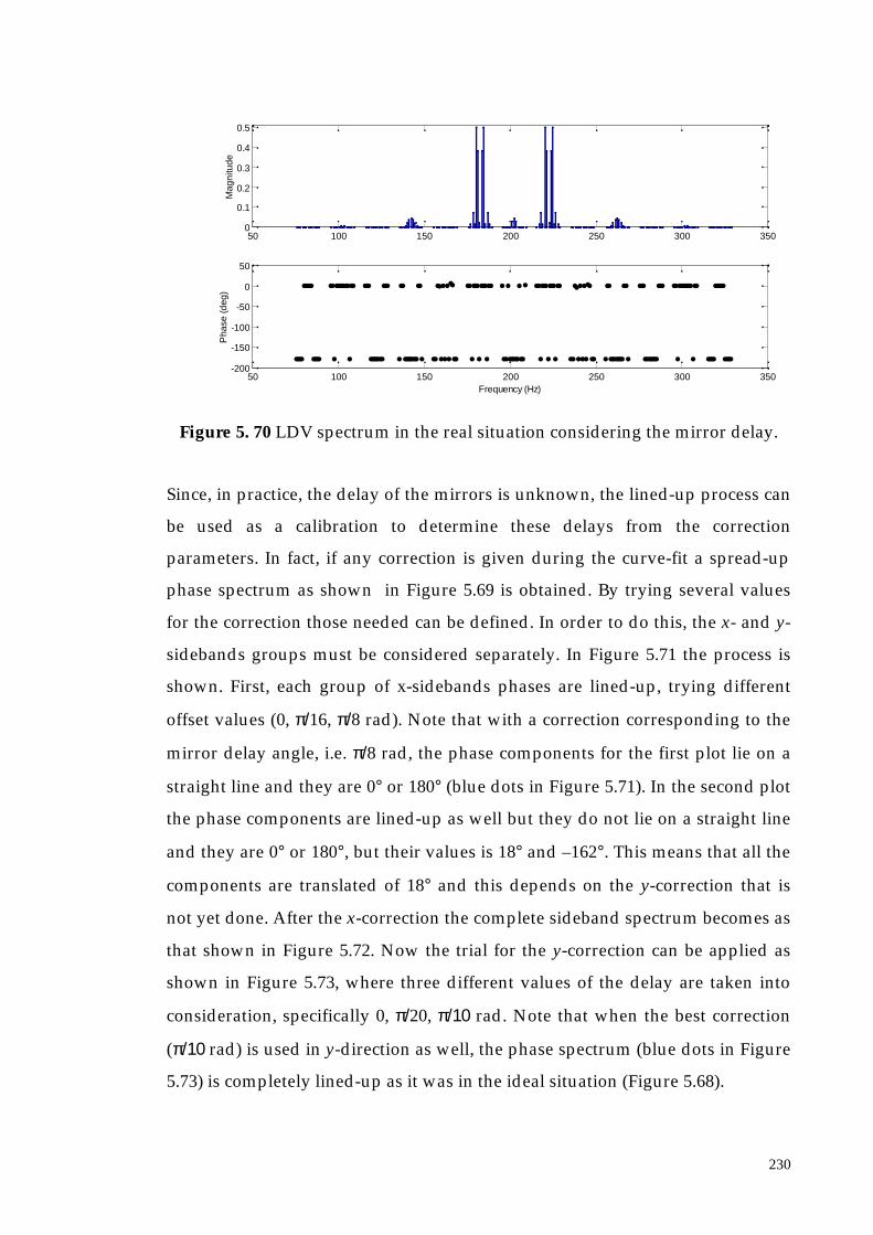
230

50 100 150 200 250 300 3500

0.1

0.2

0.3

0.4

0.5

Mag

nitu

de

50 100 150 200 250 300 350-200

-150

-100

-50

0

50

Frequency (Hz)

Pha

se (d

eg)

Figure 5. 70 LDV spectrum in the real situation considering the mirror delay.

Since, in practice, the delay of the mirrors is unknown, the lined-up process can

be used as a calibration to determine these delays from the correction

parameters. In fact, if any correction is given during the curve-fit a spread-up

phase spectrum as shown in Figure 5.69 is obtained. By trying several values

for the correction those needed can be defined. In order to do this, the x- and y-

sidebands groups must be considered separately. In Figure 5.71 the process is

shown. First, each group of x-sidebands phases are lined-up, trying different

offset values (0, π/16, π/8 rad). Note that with a correction corresponding to the

mirror delay angle, i.e. π/8 rad, the phase components for the first plot lie on a

straight line and they are 0° or 180° (blue dots in Figure 5.71). In the second plot

the phase components are lined-up as well but they do not lie on a straight line

and they are 0° or 180°, but their values is 18° and –162°. This means that all the

components are translated of 18° and this depends on the y-correction that is

not yet done. After the x-correction the complete sideband spectrum becomes as

that shown in Figure 5.72. Now the trial for the y-correction can be applied as

shown in Figure 5.73, where three different values of the delay are taken into

consideration, specifically 0, π/20, π/10 rad. Note that when the best correction

(π/10 rad) is used in y-direction as well, the phase spectrum (blue dots in Figure

5.73) is completely lined-up as it was in the ideal situation (Figure 5.68).

231

Figure 5. 71 x-group sidebands correction using different values for the mirror

delay.

50 100 150 200 250 300 350-300

-250

-200

-150

-100

-50

0

50

100

Frequency (Hz)

Pha

se (d

eg)

Figure 5. 72 Complete phase spectrum after the x-correction procedure.

195 200 205 210-300

-250

-200

-150

-100

-50

0

50

100

Frequency (Hz)

Pha

se (d

eg)

215 220 225 230-300

-250

-200

-150

-100

-50

0

50

100

Frequency (Hz)

Pha

se (d

eg)

Frequency(Hz)

First groupof x-sidebands

Secondgroup of x-sidebands

Mirror delay = 0 rad

Mirror delay = π /16 rad

Mirror delay = π / 8 rad

232

Figure 5. 73 y- correction using different values for the mirror delay.


5.5.4.3.1 Experimental Set-up Description

An experimental procedure to derive a two-dimensional area-scan ODS is now

addressed in order to demonstrate the validity of the process hereby analysed.

With reference to the test rig described in Figure 5.51 (i.e. cantilever plate with

shaker attached on it rear surface), an area scan over the surface of the structure

vibrating at a specific, known frequency, has been performed. The software

used to set up the test and to acquire and post-process the measurement data

consists of a set of LabVIEW programs whose philosophy can be summarised in

brief:

1. Set Mirrors Drivers to make the mirrors scan the area to be tested (see

Appendix A.1.5 for the control panel of the LabVIEW program driving the

mirrors).

2. Set Arbitrarily Waveform Generator parameters according to the excitation

input required (see Appendix A.1.1 for the control panel of the LabVIEW

program driving the shaker).

50 100 150 200 250 300 350-300

-250

-200

-150

-100

-50

0

50

100

Frequency (Hz)

Pha

se (d

eg)

Mirror delay = 0 radMirror delay = π/20 radMirror delay = π/10 rad

233

3. Spectral Analysis. The LDV output spectrum is visualised in order to

determine the number of the relevant sidebands present on it. The order of

the polynomial, which will represent the ODS of the tested surface, can,

then, be straightforwardly derived at this stage (see Appendix A.1.6 for the

control panel of the LabVIEW program used as spectrum analyser).

4. Data Acquisition. The signals stored for post processing are: LDV output,

which contains the surface velocity information, sinewave driving the x-

mirror, sinewave driving the y-mirror and, optionally, the force cell signal

(see Appendix A.1.3 for the control panel of the LabVIEW program used for

the acquisition).

5. ODS determination using the settings defined previously and the data

stored in the data acquisition step. The goal of this stage is to produce a plot

of the deflected surface at the excitation frequency (see Appendix A.1.7 for

the control panel of the LabVIEW program performing the post-processing

of the LDV output signal in order to derive the ODS).

By applying the LabVIEW control-acquisition programs, the plate was tested at

two frequencies of maximum response that were established by discrete

scanning technique using the conventional Polytec PSV procedure, i.e. at 202.5

Hz (4th resonance) and 241.25 Hz (5th resonance).

The LDV mirrors were set in such a way as to describe a non-closed Lissajou

pattern on the plate surface, perpendicular to the laser beam. The x-mirror was

fed with a sine wave at 1.1 Hz and the y-mirror with a sine wave at 20 Hz (i.e.

not an integral multiple of 1.1Hz). The amplitudes of these output signals were

adjusted so that the whole surface was swept by the measurement beam. The

acquisition took 10 seconds, i.e. 11 cycles of the laser beam in the direction

scanned at lower speed (1.1 Hz in the x-direction) were covered.

234

5.5.4.3.2 Test on the Plate at the Fourth Resonance

By exciting the plate at the first frequency mentioned (202.5 Hz), the LDV

output time history triggered with the sinewave driving one of the mirrors was

stored together with the excitation force signal and the two mirror drive signals.

These signals are shown in Figure 5.74, where a zoom of the acquisition start

point (zero time instant) is given in order to illustrate that the trigger is

performed with the x-mirror drive signal (red), which start at zero amplitude

with positive slope.

Figure 5. 74 Measured time signals and zoom on the acquisition initial time

instant which shows that the trigger signal employed is the x-

mirror driver signal (red line).

The acquisition sample rate must be carefully chosen as it should be higher than

twice the highest frequency component of the LDV output spectrum. This latter

would be given by:

201.15.202 ×+×+ mn

0 0.5 1 1.5

-4

-3

-2

-1

0

1

2

3

4

Time (s)

Acq

uire

d T

ime

His

torie

s (V

)

LDV Output Signal x-mirror Drive Signaly-mirror Drive Signa

ZOOM OUT

235

n and m being the number of x- and y-sidebands that should be chosen in the

curve-fit process. Say that n = m = 8, the maximum frequency would be 371.3

Hz and the sample rate at least 750 Hz.

By observing the LDV signal spectrum (Figure 5.75) the number of x- and y-

sidebands necessary to be taken into account in the curve-fitting process can be

decided. It was noticed, that some small amplitude peaks were present in a high

frequency region – above the group being considered here. Zooming in on this

range (Figure 5.76) it is easy to see that these components are centered at 405

Hz, which is the second harmonic of the excitation frequency. This

phenomenon is due to speckle noise, see Subsection 2.5, and if the beam was

better focused, i.e. the beam width w of light used for illumination was smaller,

the effect might be much reduced, or even disappear altogether. The

phenomenon does not affect the analysis and can be neglected.

0 100 200 300 400 500 6000

0.1

0.2

0.3

0.4

0.5

Frequency (Hz)

Spe

ctru

m M

agni

tude

(V

)

Figure 5. 75 LDV Output Spectrum.

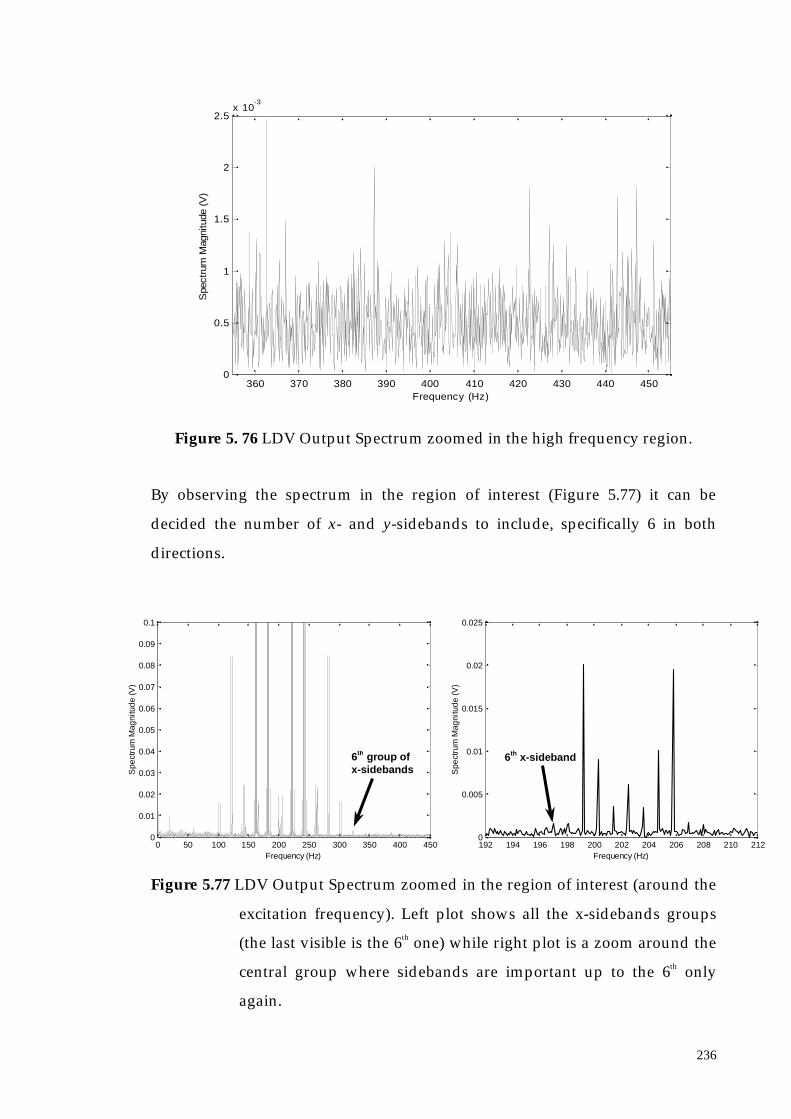
236

360 370 380 390 400 410 420 430 440 4500

0.5

1

1.5

2

2.5x 10

-3

Frequency (Hz)

Spe

ctru

m M

agni

tude

(V

)

Figure 5. 76 LDV Output Spectrum zoomed in the high frequency region.

By observing the spectrum in the region of interest (Figure 5.77) it can be

decided the number of x- and y-sidebands to include, specifically 6 in both

directions.

Figure 5.77 LDV Output Spectrum zoomed in the region of interest (around the

excitation frequency). Left plot shows all the x-sidebands groups

(the last visible is the 6th one) while right plot is a zoom around the

central group where sidebands are important up to the 6th only

again.

0 50 100 150 200 250 300 350 400 4500

0.01

0.02

0.03

0.04

0.05

0.06

0.07

0.08

0.09

0.1

Frequency (Hz)

Spe

ctru

m M

agni

tude

(V)

192 194 196 198 200 202 204 206 208 210 2120

0.005

0.01

0.015

0.02

0.025

Frequency (Hz)

Spe

ctru

m M

agni

tude

(V)

6th group ofx-sidebands

6th x-sideband

237

By curve-fitting the LDV time history at the frequencies of

201.15.202 ×±×± mn , for n and m assuming integer values from 0 up to 6. In

order to have a phase spectrum with aligned components, the mirror delays

must be considered; after some trials it was found that the best configuration

was obtained when the delay associated with the x-mirror was 0.53 rad (δx) and

the one associated with the y-mirror was 0.803 rad (δy). The curve fit was then

performed by multiplying by sine and cosine of

yx mnmn δδ ×±×±×±×± 201.15.202 . Figure 5.78 shows the amplitude and

phase spectrum recovered. Note, that the phase spectrum is still spread, even

taking into account the mirrors delay. This occurs because the actual ODS of the

plate is not completely real. In fact, observing the complex LDV output

spectrum, Figure 5.79, it can be seen that the real and imaginary components

are comparable.

50 100 150 200 250 300 3500

0.2

0.4

0.6

0.8

Am

plitu

de (V

)

50 100 150 200 250 300 350-250

-200

-150

-100

-50

0

Frequency (Hz)

Pha

se (d

eg)

Figure 5. 78 LDV output spectrum in magnitude and phase format.

238

50 100 150 200 250 300 350

-0.2

-0.1

0

0.1

0.2

0.3

Rea

l Com

pone

nt (V

)

50 100 150 200 250 300 350-0.4

-0.2

0

0.2

0.4

Frequency (Hz)

Imag

inar

y C

ompo

nent

(V)

Figure 5. 79 Real and imaginary components of the LDV output spectrum.

From the LDV output spectrum, in terms of real and imaginary components,

sidebands matrices ARnm and AInm can be derived. Applying to these the [T]

transform (Equation (5.54) ) real and imaginary polynomial coefficients series

VRnm and VInm are established and the real and imaginary components of the ODS

can be plotted as shown in Figure 5.80 and 5.81 respectively.

Figure 5. 80 Plate ODS real component.

y

x

CANTILEVER EDGE

239

Figure 5. 81 Plate ODS imaginary component.

In order to obtain a purely real ODS, the phase can be adjusted to minimise the

output to effectively give zero imaginary parts of the ODS and then, shifted by

π/2 to give the real component. This procedure is useful when the mode shape

complexity, or lack of it, is to be demonstrated. The phase is then referred to one

relative to the maximum imaginary component of the spectrum shown in

Figure 5.79. Figures 5.82 and 5.83 show respectively the amplitude and

translated phase spectrum and the complex spectrum recovered, specifically the

in-phase and out-of-phase components.

50 100 150 200 250 300 3500

0.2

0.4

0.6

Am

plitu

de (V

)

50 100 150 200 250 300 350-300

-200

-100

0

100

Frequency (Hz)

Pha

se (d

eg)

Figure 5.82 Amplitude and Phase spectrum of the LDV output obtained for

imaginary component minimising.

x

y

CANTILEVER EDGE

240

50 100 150 200 250 300 350

-0.4

-0.2

0

0.2

0.4

0.6

In-p

hase

Com

pone

nt (V

)

50 100 150 200 250 300 350-3

-2

-1

0

1

2x 10

-3

Frequency (Hz)

Out

-of-p

hase

Com

pone

nt (V

)

Figure 5.83 In-phase and Out-of-phase components of the LDV output

spectrum.

The ODS in-phase and out-of phase components are illustrated in Figure 5.84.

Note that the ODS now represents the velocity pattern since it is given in

mm/s. In fact, the polynomial coefficient series were multiplied by the laser

sensitivity (5 mm/s/V) in order to have a response mode shape, comparable

with the velocity pattern derived by using the conventional discrete area

scanning technique, provided by the Polytec system (See Figure 5.52). Figure

5.85 shows both the ODSs at 202.5 Hz derived with Polytec and the continuous

area scan.

Figure 5. 84 Vibration pattern from the contiuous area scan at 202.5 Hz.

In-phase ODS Out-of-phase ODS

241

Figure 5. 85 Vibration patterns at 202.5 Hz from continuous area scan and the

conventional Polytec step-point area scan.

A validation parameter similar to the Modal Assurance Criterion (MAC) was

calculated between the ODS derived by continuous area scan (C) and discrete

area scan (D) following the MAC definition:

( )∑∑∑∑

∑∑

= == =

= ==n

i

m

jji

n

i

m

jji

n

i

m

jjiji

DC

DC

MAC

1 1

2

1 1

2

1 1, DC (5. 66)

where the sums are done for each point of the mode shape surface (then if the

ODS is defined for x = -1..0.02..1 and y = -1..0.02..1, n = m= 101). Note that the

ODS were found to be purely real, therefore no complex notation is used in the

MAC equation (5.66). The MAC value obtained was 87 %.

To validate the results the theoretical mode derived analytically by employing

the theory for uniform plates, [38], was calculated using Equation (5.57) and its

plot is shown in Figure 5.86. The MAC between theoretical mode and ODS from

ODS from continuous area scan ODS from discrete area scan

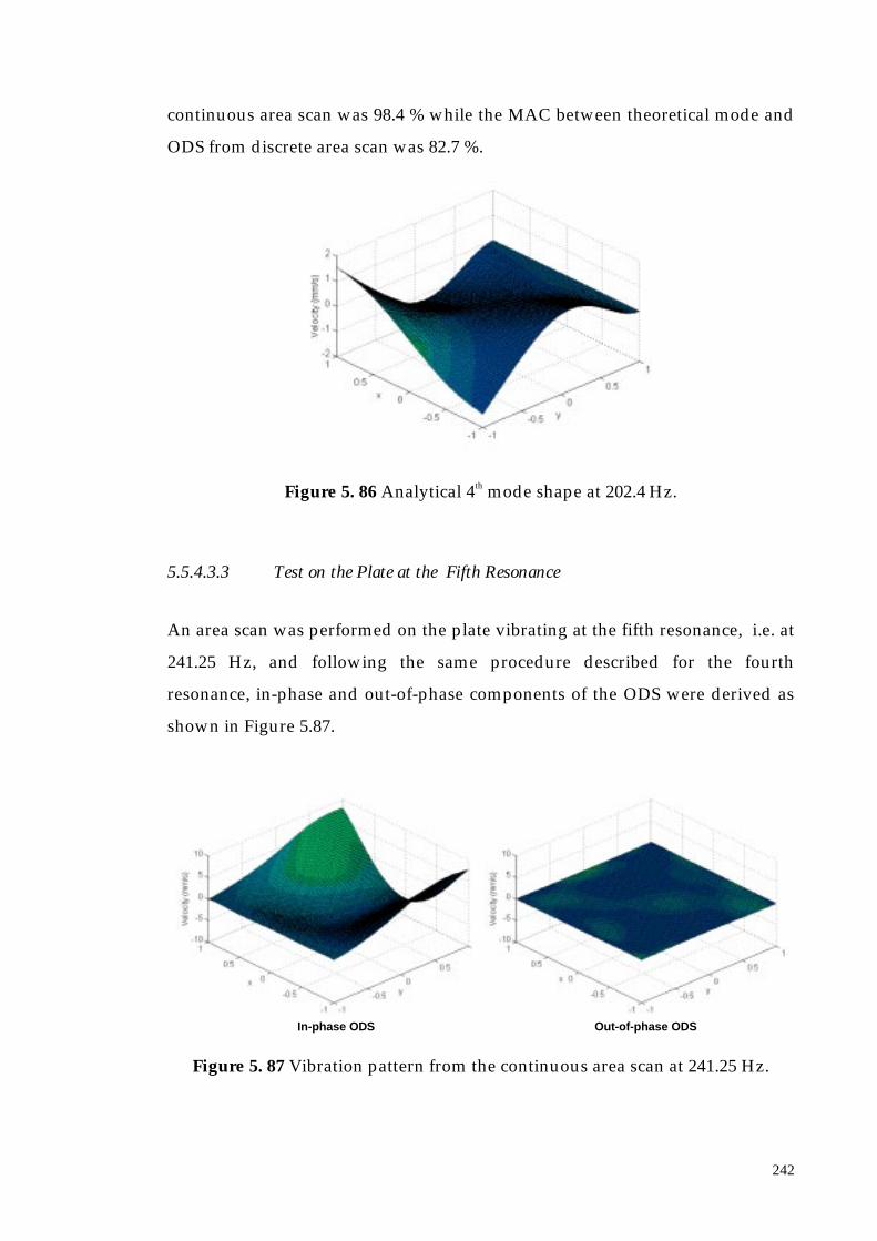
242

continuous area scan was 98.4 % while the MAC between theoretical mode and

ODS from discrete area scan was 82.7 %.

Figure 5. 86 Analytical 4th mode shape at 202.4 Hz.

5.5.4.3.3 Test on the Plate at the Fifth Resonance

An area scan was performed on the plate vibrating at the fifth resonance, i.e. at

241.25 Hz, and following the same procedure described for the fourth

resonance, in-phase and out-of-phase components of the ODS were derived as

shown in Figure 5.87.

Figure 5. 87 Vibration pattern from the continuous area scan at 241.25 Hz.

In-phase ODS Out-of-phase ODS

243

For comparison, the corresponding ODS was recovered from the stepped area

scan which was done using the conventional Polytec facilities. In Figure 5.88 the

ODSs derived with both techniques are shown.

The MAC parameter derived from the correlation between Polytec and

continuous area scan results was 85.27 %. Again, the theoretical mode shape

was determined and the correlation performed with the continuous area scan

ODS first, and then with the discrete area scan. The MAC values derived were

respectively 95.17 and 88.06 %. Figure 5.89 is the plot of the analytical mode

shape at 242.68 Hz (see Table 5.7).

Figure 5. 88 Vibration patterns at 241.25 Hz from continuous area scan and the

conventional Polytec step-point area scan.

Figure 5. 89 Analytical 5th mode shape at 242.68 Hz.

ODS from continuous area scan ODS from discrete area scan

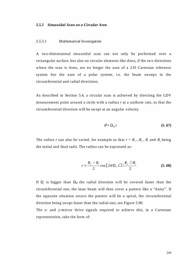
244

5.5.5 Sinusoidal Scan on a Circular Area


A two-dimensional sinusoidal scan can not only be performed over a

rectangular surface, but also on circular elements like discs, if the two directions

where the scan is done, are no longer the axes of a 2-D Cartesian reference

system but the axes of a polar system, i.e. the beam sweeps in the

circumferential and radial directions.

As described in Section 5.4, a circular scan is achieved by directing the LDV

measurement point around a circle with a radius r at a uniform rate, so that the

circumferential direction will be swept at an angular velocity

tθθ Ω= (5. 67)

The radius r can also be varied, for example so that r = Ri....Rf , Ri and Rf being

the initial and final radii. The radius can be expressed as:

( )2

2cos2

ifr

if RRt

RRr

++

−= Ωπ (5. 68)

If Ωr is bigger than Ωθ the radial direction will be covered faster than the

circumferential one, the laser beam will then cover a pattern like a “daisy”. If

the opposite situation occurs the pattern will be a spiral, the circumferential

direction being swept faster than the radial one, see Figure 5.90.

The x- and y-mirror drive signals required to achieve this, in a Cartesian

representation, take the form of:

245

( ) ( )

( ) ( )tRRt

RRy

tRR

tRR

x

ifr

if

ifr

if

θ

θ

ππ

ππ

ΩΩ

ΩΩ

2sin2

2cos2

2cos2

2cos2

++

−=

++

−=

(5. 69)

Figure 5. 90 Laser beam pattern on a disc-like component for circumferential

speed (1.1 Hz) lower than the radial (20 Hz) (left), and vice versa

(right).

If the vibration pattern of the disc surface can be written as:

( ) ( ) ( ) ( ) ( ) ( ) ( )tnrvtnrvtrv InRn ωθωθθ sinsincoscos,, += (5. 70)

and specifically, the radial mode shape may be expressed as a polynomial of the

pth order, then:

( )

( ) ∑

∑

=

=

=

=

p

i

iiInIn

p

i

iiRnRn

rVrv

rVrv

0

0 (5. 71)

y

x

y

x

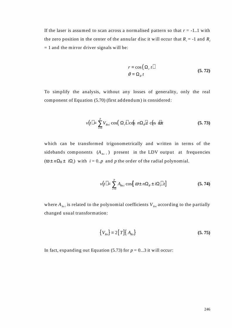
246

If the laser is assumed to scan across a normalised pattern so that r = -1..1 with

the zero position in the center of the annular disc it will occur that Ri = -1 and Rf

= 1 and the mirror driver signals will be:

( )t

tr r

θθ ΩΩ

== cos

(5. 72)

To simplify the analysis, without any losses of generality, only the real

component of Equation (5.70) (first addendum) is considered:

( ) ( ) ( ) ( )∑=

=p

ir

iiRn ttntVtv

0

coscoscos ωθΩΩ (5. 73)

which can be transformed trigonometrically and written in terms of the

sidebands components (ARn i ) present in the LDV output at frequencies

(ω ± nΩθ ± iΩr) with i = 0..p and p the order of the radial polynomial.

( ) ( )[ ]∑=

±±=p

iriRn tinAtv

0

cos ΩΩθω (5. 74)

where ARn i is related to the polynomial coefficients VRni according to the partially

changed usual transformation:

[ ] RnRn ATV 2= (5. 75)

In fact, expanding out Equation (5.73) for p = 0...3 it will occur:

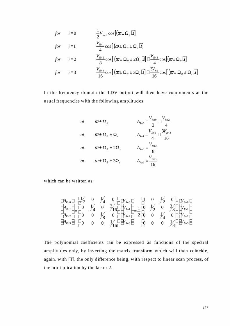
247

( )[ ]

( )[ ]

( )[ ] ( )[ ]

( )[ ] ( )[ ]tVt

Vifor

tV

tV

ifor

tV

ifor

tVifor

rR

rRn

Rnr

Rn

rRn

Rn

ΩΩΩΩ

ΩΩΩ

ΩΩ

Ω

±±+±±=

±+±±=

±±=

±=

θθ

θθ

θ

θ

ωω

ωω

ω

ω

cos16

33cos

163

cos4

2cos8

2

cos4

1

cos2

10

33

22

1

0

In the frequency domain the LDV output will then have components at the

usual frequencies with the following amplitudes:

163

82

16

3

4

42

33

22

311

200

RnRnr

RnRnr

RnRnRnr

RnRnRn

VAat

VAat

VVAat

VVAat

=±±

=±±

+=±±

+=±

ΩΩ

ΩΩ

ΩΩ

Ω

θ

θ

θ

θ

ω

ω

ω

ω

which can be written as:

=

=

3

2

1

0

3

2

1

0

3

2

1

0

81000

04100

8302

10

02101

2

1

161000

08100

16304

10

04102

1

Rn

Rn

Rn

Rn

Rn

Rn

Rn

Rn

Rn

Rn

Rn

Rn

V

V

V

V

V

V

V

V

A

A

A

A

The polynomial coefficients can be expressed as functions of the spectral

amplitudes only, by inverting the matrix transform which will then coincide,

again, with [T], the only difference being, with respect to linear scan process, of

the multiplication by the factor 2.

248


In order to simulate the vibration velocity experienced by the laser beam when

it scans over the plane surface of a disc, the theory of thin discs (i.e. rotational

inertia and shear effects are neglected) is taken into analysis. Specifically, the

disc is an annular plate of internal radius 0.015 m and external radius of 0.15 m

and it is clamped on the inside. The specimen is shown in Figure 5.91 with

reference to a polar coordinate system with the origin coincident with the center

of the disc. This configuration is the most common to find in practice, when an

axi-symetric disc is fixed to a rotating shaft.

Figure 5. 91 Annular disc clamped on inside and free on outside.

The solution of the equation of the disc transverse vibrations is given in

reference [38] and, after some simplifications (i.e. the origin of the polar

reference system coincides with the disc center and the boundary conditions

possess symmetry with respect to one or more diameters of the disc), can be

written as:

( ) ( ) ( )[ ] ( )∑∞

=

+=0

cos,n

nnnn nkrICkrJArw θθ (5. 76)

where Jn is the Bessel function of the first kind,

In is the modified Bessel function of the first kind,

n = 0, 1, ... ∞ is the number of nodal diameters (diametral lines

where the vibration is zero) of the mode shape,

r

θ

Ri Rf

249

k is a factor depending on the natural frequency associated with

the mode shape so that D

hk

ρω=2 , where ρ is the mass density

of the disc, h is its thickness and D is the flexural rigidity, and

An, Cn are constants to be established by defining the boundary

conditions on both the disc edges.

For a typical mode n, the radial component of the mode shape can be expressed

as:

( ) ( ) ( )krICkrJArw nnnnn += 5. 77

and it must be understood that n can take all values from 0 to ∞.

If the inside radius (Ri ) of the disc is clamped all around, the boundary

conditions at r = Ri for every values of θ will be:

( )( )

0

0

=

=

= iRr

i

dr

rdw

Rw

5. 78

By introducing Equation (5.77) in (5.78), the existence of a non-trivial solution

yields the characteristic equation:

( ) ( ) ( ) ( ) 011 =+ ++ inininin kRJkRIkRIkRJ 5. 79

The eigenvalues kRi can be obtained by solving Equation (5.79) but they are

tabulated [38] Considering a disc with an inside radius of 0.015m and an

outside radius of 0.15 m (Ri /Rf = 0.1) and assuming the mode shape to have 2

250

nodal diameters (n) and one nodal circumference (s) (i.e. circle where the

vibration is zero), the value of D

hRi

ρωλ 22 = is 37 and then 0828.6== λikR .

The mode shapes of Equation (5.77) are determined from either Equations

(5.78). Using the first equation the constants ratio will be derived:

0014.1)(

)( −=−=in

in

n

n

kRJ

kRI

C

A(5. 80)

The radial mode shape ( Equation (5.77) ) becomes then:

( ) ( ) ( )rIrJrw nnn 0828.60828.60014.1 +−= (5. 81)

which is shown in Figure 5.92.

Figure 5. 92 Radial mode shape.

The complete mode shape is given by Equation (5.76):

( ) ( ) ( )[ ] ( )θθ 2cos0828.60828.60014.1, rIrJrw nnn +−= (5. 82)

Ri Rf

w(r)

r

251

and this is shown in Figure 5.93.

Figure 5. 93 Mode shape of the disc with two nodal diameters and one nodal

circumference.

In order to make it possible to apply the Fourier transform to the LDV output

when this scans all over the disc surface and to recover from it the ODS of the

disc itself, the mode shape must be written as a polynomial. The radial mode

shape is then approximated by a 4th order polynomial and the two-dimensional

mode shapes can be rewritten as:

( ) ( )θθ 2cos]0151.7000063543.00046211.0021623.063.28[, 7234 −+−−−= errrrrw

(5. 83)

If now an LDV scan is performed across the disc surface undergoing this

vibration pattern, the laser beam will output a velocity signal of the form:

( )( ) ( )t

errrrtv

ωπθ 2cos2cos

]0151.7000063543.00046211.0021623.063.28[ 7234 −+−−−= (5. 84)

r

θ

w(r,θ)

252

which is exclusively dependent on the time coordinate, r and θ being given by

Equations (5.68) and (5.67).

The natural frequency, ω, can be determined from knowledge of the tabulated

parameter, 372 22 ==D

hRi

ρωπλ , D being Eh3/12 (1-ν 2). Assuming the disc is

made from aluminum (E = 6.75 e10 N/m2 and ρ = 2640 kg/m3) and its thickness

is 0.005 m the natural frequency will be 2026 Hz.

First, the laser beam is supposed to follow a spiral pattern at a circumferential

speed of 20 Hz and a radial speed of 1.1 Hz; the LDV time history is shown then

in Figure 5.94and its Fourier spectrum in Figure 5.96. If, successively, the laser

is considered to perform a daisy on the disc surface with circumferential and

radial speed reversed the LDV output time history and spectrum will become

as shown in Figure 5.95 and 5.97.

Figure 5. 94 LDV output time history when the laser beam scans in a spiral


frequency of 2026 Hz. The zoom shows clearly the signal

modulation given by the circumferential motion of the laser beam.

0 0.5 1 1.5 2

-0.015

-0.01

-0.005

0

0.005

0.01

0.015

Time (s)

Vel

ocity

(m/s

)

LDV output Radial Position Driver Signal

ZOOMIN

253

0 0.2 0.4 0.6 0.8 1 1.2 1.4 1.6 1.8 2-0.02

-0.015

-0.01

-0.005

0

0.005

0.01

0.015

0.02

Time (s)

Vel

ocity

(m/s

)

LDV output Radial Position Signal Driver

Figure 5. 95 LDV output time history when the laser beam scans in a daisy


frequency of 2026 Hz. The modulation due to the circumferential

motion of the laser beam is visible.

1980 1990 2000 2010 2020 2030 2040 2050 2060 2070 20800

0.2

0.4

0.6

0.8

1

1.2

1.4

1.6

1.8

2x 10

-3

Frequency (Hz)

Spe

ctra

l Am

plitu

de (m

/s)

Figure 5. 96 LDV output time history when the laser beam scans over a spiral

pattern on the surface of the disc vibrating at the natural

frequency of 2026 Hz.

When the laser beam scans in a spiral pattern the circumferential direction is

swept at the speed of 20 Hz. Two groups of sidebands then appear spaced of 20

× 2 = 40 Hz from the excitation frequency since the nodal diameters are two.

254

Each group is formed by 4 pairs of sidebands 1.1 Hz (the radial speed) apart

from each other, the radial polynomial mode shape being of the 4th order.

1900 1950 2000 2050 2100 21500

0.2

0.4

0.6

0.8

1

1.2

1.4

1.6

1.8

2x 10

-3

Frequnecy (Hz)

Spe

ctra

l Am

plitu

de (m

/s)

Figure 5. 97 LDV output time history when the laser beam scans in a daisy


frequency of 2026 Hz.

Now the LDV spectrum consists of four pairs of sideband groups spaced 20 Hz

(the radial frequency) from each other and each group then contains 2

sidebands spaced apart by 1.1 × 2 = 2.2 Hz, where 1.1 Hz is the circumferential

speed, in which direction two nodal diameters are present.

The LDV output time history is then post-processed in the usual way by being

multiplied by sine and cosine functions at frequencies (2026 ± 2 × 1.1 ± i × 20),

considering the laser beam performing a daisy (LDV output spectrum shown in

Figure 5.99), for i = 0...4. The LDV spectral components derived are depicted in

amplitude and phase in Figure 5.98 and they are:

An = 2.071 e-3 1.607 e-3 7.347 e-4 1.814 e-4 1.885 e-4

255

1940 1960 1980 2000 2020 2040 2060 2080 2100 21200

0.5

1

1.5

2

2.5x 10

-3

Am

plitu

de (m

/s)

1940 1960 1980 2000 2020 2040 2060 2080 2100 2120

-50

0

50

Frequency (Hz)

Pha

se (d

eg)

Figure 5. 98 Curve fitted LDV output spectrum in amplitude and phase.

By applying to the sidebands amplitude vector to the transformation shown in

Equation 5.75, the polynomial coefficients series Vn i can be recovered:

Vn = 1.278 e-3 4.252e e-3 5.274 e-3 2.903 e-3 6.034 e-4

The polynomial representing the radial mode shape can be derived, bearing in

mind, that the radial position is normalised between –1 and 1, instead of going

from the true dimensions of the disc (0.015 and 0.15 m). Then, if the spatial

position is defined as x = -1...1, in order to recover the same plot as Figure 5.93

with r = 0.015...0.15 the radial mode shape should be written as

( ) ( ) ( )( ) ( ) 4323

3343

034.6815.14222.1903.2815.14222.1274.5

815.14222.1252.4815.14222.1287.1−−−

−−

++−−+−+

++−−+−=

erere

rererw

which can be approximated by a polynomial of r only :

( ) ]88.50005.00082.01522.00720.29[ 6234 −+−−−= errrrrw

This radial mode shape can be compared with the one given by Equation (5.81)

which is the original and is shown in Figure 5.92.

256

The two dimensional disc mode shape is finally given by

( ) ( )θθ 2cos]88.50005.00082.01522.00720.29[, 6234 −+−−−= errrrrw

which completely matches the original mode shape given by Equation (5.82)

and shown in Figure 5.93.


As a practical example of circular area scans, a laboratory test was performed

on the pin-on-disc rig described in Section 5.4, Figure 5.42, with the pin

retracted and with direct excitation at a relevant 3d-diameter mode resonance

frequency (2271 Hz). The scan across the disc surface was achieved by driving

the LDV mirrors by signals given by Equation (5.69) at the frequencies of 20 and

1.1 Hz and with external radius (Rf ) coincident with the disc actual radius (0.406

m) and the internal one (Ri ) as large as the bolt fixing the disc on the shaft could

be avoided (i.e. 0.025 m). Under these conditions, the total time required by the

laser scanning beam to cover the whole disc annular surface is about 1 sec, since

the time to perform one cycle in the lower-speed (1.1 Hz) direction is 0.0909

secs. First a daisy pattern (Ωr bigger than Ωθ) was produced and the LDV

spectrum obtained is shown in Figure 5.99.

2220 2230 2240 2250 2260 2270 2280 2290 2300 2310 23200

0.05

0.1

0.15

0.2

0.25

0.3

Frequency (Hz)

Magn

itude

(V)

Figure 5. 99 LDV signal spectrum for the daisy scan and excitation at 2271 Hz.

257

The LDV spectrum consists of only two sideband pairs on either side of the

central pair, so that the radial distribution derived, will simply be a quadratic

expression in r. Moreover, each group of sidebands is split in two, the spacing

between each pair being ± 3 Ωθ . Spectral components are then located at 2271 ±

3 × 1.1 ± i × 20 Hz, with i = 0, 1 and 2. They are shown, averaged out with

respect to the central frequency, i.e. the excitation frequency 2271 Hz, in Figure

5.100.

2220 2230 2240 2250 2260 2270 2280 2290 2300 2310 23200

0.1

0.2

0.3

0.4

Am

plitu

de (V

)

2220 2230 2240 2250 2260 2270 2280 2290 2300 2310 2320

-50

0

50

Frequency (Hz)

Pha

se (d

eg)

Figure 5. 100 Sidebands spectral components of the LDV output.

The sideband matrix An can then be recovered, considering only the radial

components at 2271 + 3 × 1.1 ± i × 20 Hz. All of these will have the same sign

(i.e. positive), the sideband components being in phase with each other:

An = 0.3160 0.2192 0.0629 (V)

By applying the transformation in Equation (5.75), the polynomial coefficients

can be recovered and by multiplying by the LDV velocity range (5 mm/s/V)

they can be expressed in terms of velocity:

Vn = 1.9005 4.3846 2.5196 (mm/s)

258

Then the radial mode shape will be

( ) 9005.13846.45196.2 2 ++= rrrw

which is plotted, for a normalised radial position (r = -1...1), in Figure 5.101.

-1 -0.5 0 0.5 1-1

0

1

2

3

4

5

6

7

8

9

Radial Position

Vel

ocity

Pat

tern

(mm

/s)

Figure 5. 101 Radial ODS at 2271 Hz along the radius of the annular disc.

The global ODS will be:

( ) ( ) ( )θθ 3cos9005.13846.45196.2, 2 ++= rrrw

which is plotted against the true dimension of the annular disc in Figure 5.102.

259

Figure 5. 102 Two-dimensional ODS at 2271 Hz.

By performing a spiral pattern scan across the annular disc surface by

substituting the radial frequency with the circumferential (i.e. Ωr = 1.1 Hz and

Ωθ = 20 Hz), and following the same procedure, an identical two-dimensional

ODS can be recovered. The LDV output spectrum is shown in Figure 5.103.

2200 2220 2240 2260 2280 2300 2320 23400

0.05

0.1

0.15

0.2

Frequency (Hz)

Mag

nitu

de (V

)

Figure 5. 103 LDV signal spectrum for the spiral scan and excitation at 2271 Hz.

260

5.6. Modal Analysis of ODSs derived by Area Scan

5.6.1 Introduction

The CSLDV methods described in the previous sections give response

measurements for sinusoidal excitation at a single frequency and yield real and

imaginary ODSs to be recovered as polynomial series, over the area being

scanned. If the process is repeated at a series of frequencies, with sufficient

frequency resolution, as in a stepped-sine test, frequency response functions can

be established over this range. By applying any conventional modal analysis

process to these FRFs, natural frequencies, modal damping factors and modal

constants may be evaluated. The modal analysis procedure can be applied to

the sideband responses referred to the measured input force directly. These

represent weighted summations of responses which form the eigenvectors in

just the same way as any other grouping of DOFs, i.e. measured points on the

structure which now corresponds to the sidebands on the spectrum, the latter

giving the spatial information. The processing necessary to derive series

coefficients for ODSs is then performed on the modal constants in order to

obtain, this time, mode shapes, again as polynomial series. If multiple FRFs

have been acquired by a sinusoidal area scan over a whole surface, this

represents a considerable saving because a global modal analysis algorithm

may be applied to the complete set of scan data.

It must be pointed out that the modal analysis process is, in this case, applied to

sidebands referred to a derived natural frequency which is artificially translated

by the scan procedure, i.e. for the n,m sideband the natural frequency

will be (ωr + nΩx + mΩy) where ωr is the true natural frequency. This means that

the “natural frequencies” derived from sideband FRFs are shifted by nΩx + mΩy.

In consequence, estimates of modal damping factors and modal constants have

to be multiplied by ( ) ( )

22

22

ωωωω

−++−++

r

yxyxr mnmn ΩΩΩΩ.

261

In fact, the modal analysis procedure consists of applying the following formula

to derive the modal constant, see reference [1]

( ) ∑= +−

=N

r rrr

jkrjk

i

AH

1222 ωηωω

ω (5. 85)

where Hjk is the FRF measured at the point j that now is the sideband

location, i.e. j = i,l with i= 0 ... n and l= 0 ... m and k is the

excitation point which is unique, the excitation being position

in only one point;

r Ajk is the modal constant relative to the jth (i.e. n,m) sideband

FRF again k being constant;

ωr the natural frequency of the natural mode included within

the frequency range ω analysed, which usually is in the

neighborhood of a maximum response frequency and then of

the natural frequency;

ηr the damping loss factor.

This relationship is exact in the case of the first FRF associated with the

excitation frequency, which is not translated by the x- and y-scan speeds, but for

the other FRFs corresponding to the sidebands this translation must be taken

into account.

An example may clarify the somewhat unusual perspective on modal testing

illustrated above.

5.6.2 Experimental Modal Analysis on the Garteur Structure

A laser Doppler vibrometer was used to perform a continuous scan over a

particular test piece, the GARTEUR structure, used as a test case for evaluating

modal testing methods and FE analysis capabilities, see reference [19]. The

262

GARTEUR structure is a high-tail aircraft model, consisting of a beam assembly

as shown in Figure 5.104. The dimension of the wing span is 2 m.

Figure 5. 104 The GARTEUR structure.

The structure was hung from the ceiling with the tail on top. The front surface

of the wing was scanned by the LDV and the excitation was applied from

behind, at one end of and perpendicular to the wing surface, see in Figure 5.105.

Figure 5. 105 Excitation and LDV continuous-scan path.

y

x

AREA SCAN PATTERN

EXCITATION POINT

263

The frequency range excited (30-40 Hz) was chosen so as to include a specific

natural frequency of one of three close natural modes which had been located

by performing a finite element analysis on the structure. These modes, all

involving out-of-plane vibration of the wing part of the structure, have a

predominantly wing bending mode at 32.58 Hz, a symmetric wing torsion at

33.11 Hz, and a skew-symmetric wing torsion at 33.38 Hz.

In the experimental set-up the structure was hung nose-down, so that the LDV

could be directed at any point on the wing almost perpendicularly to measure

its z-axis vibration. Response measurements were obtained with the LDV

scanning over an area encompassing both wings, with an x-axis sinusoidal scan

at 0.3 Hz (Ωx), and a simultaneous y-axis scan (Ωy) at 5.0 Hz. The frequency-

domain spectrum of the LDV, then contains components at all frequencies

(ω ± nΩx ± mΩy), from which coefficients Vn,m for the polynomial series Σ Vn,m xn

ym giving the spatial ODS may be derived. In this case, y-axis vibration only

involved torsional-type motion, so only values of 0 and 1 needed to be included

for m while values of n up to 7 were adequate to describe the ODS along x-axis

direction.

By performing a conventional point measurement directing the laser beam in a

steady position, corresponding to the excitation point a conventional

magnitude, and phase point FRF is obtained (see Figure 5.106) which indicates

a mode at 35.0 Hz comparable with the predicted natural frequencies 32.58,

33.11 and 33.38 Hz.

0 5 10 15 20 25 30 35 40 45 50-20

0

20

40

60

Mag

nitu

de

(dB

- 0 d

B =

0.1

25 m

/s/N

)

0 5 10 15 20 25 30 35 40 45 50-150

-100

-50

0

50

100

Frequency (Hz)

Phas

e (d

eg)

Figure 5. 106 Point Mobility FRF.

264

When a continuous scan was performed over the area previously mentioned,

the maximum vibration response was found at 34.8 Hz, corresponding roughly

to the natural frequency. In order to determine the excitation frequency to have

the maximum vibration, the frequency of the signal feeding the shaker was

changed between 30 and 40 Hz and by observing the modulated LDV output

signal the excitation could be decided. The natural frequency to be excited was

the one corresponding to the excitation frequency which produces a maximum

LDV output with a more emphasised modulation. This time history is

illustrated in Figure 5.107 together with the mirror driver signals.

0 1 2 3 4 5 6 7 8 9 10-8

-6

-4

-2

0

2

4

6

Time (s)

Tim

e H

isto

ry (V

)

LDV output y-mirror Driver Signalx-mirror Driver Signal

Figure 5. 107 LDV time-signal obtained by area scan; and x-axis and y-axis

mirror drive signals.

By post-processing the time signal in the usual way, the ODS at 34.8 Hz is

recovered in order to have a basis of comparison with the corresponding mode

shape which will be obtained by performing a modal analysis procedure on the

set of measurement data acquired in the step-sine process described below. The

complex spectrum of the LDV time signal is shown in Figure 5.108 in

magnitude/phase format. It was extracted by multiplying the LDV time signal

by suitably phase-shifted (depending on the mirrors delay) sine and cosine

waves at each component frequency ( 34.8 ± n 0.3 ± m 5, with n = 0, 1 and

m = 0, ..., 7). It can be noticed that, for an ODS, the reference phase vector for

real and imaginary components is arbitrary. It can conveniently be set, as it was

265

for the illustrations here, to minimise the imaginary component. All the

components are then almost lined up at 0° and 180°. The spectrum consists of

three sidebands groups: a central one, symmetrical, which describes the wing’s

translational vibration along the x-axis, the longest dimension, and two groups,

similar to each other, spaced symmetrically about (ω + Ωy ), which describe the

torsional vibration, along the shortest dimension (y).

28 30 32 34 36 38 40 42-50

0

50

100

150

200

Frequency (Hz)

Phas

e (d

eg)

28 30 32 34 36 38 40 420

2

4

6

8

10

Mag

nitu

de

(V)

Figure 5. 108 Area scan LDV signal spectrum components.

These sideband data were processed to give 16-term polynomial equations for

real and imaginary ODS surfaces, which are plotted in Figure 5.109. This

describes a complex ODS with, predominantly, a torsion mode of the left-hand

wing, and some bending.

Figure 5. 109 Real and imaginary ODS at 34.8 Hz.

266

Now, attention is concentrated on the sine-step procedure which was

performed around the maximum response frequency of 34.8 Hz in order to

undertake a modal analysis on it and to derive the normal mode shape.

Sideband data were obtained at a series of frequencies between 33.7 and 37.7

Hz, with a 0.1 Hz step, then normalised to the input force signal and plotted to

give a set of sideband FRFs (see Appendix A.2, Figures from A.10 to A.29, for

the sideband FRFs at frequencies from 34 to 35.9 Hz, i.e. around resonance).

Note that the sideband FRF amplitudes increase in proximity to the maximum

response frequency (34.8 Hz) and the maximum amplitude is indeed reached

around this frequency (Figures A.17, A.18, A.19). A change in the phase of the

sideband FRFs can be observed as well. In fact, passing through the maximum

response frequency, the phase of each spectral component undergoes a 180°

phase shift. For instance, if attention is concentrated on the central component,

it can be seen that for frequencies smaller than 34.8 Hz, the phase assumes a

value around -50° while for higher frequencies its value is around 100°, see

Figures A.10 up to A.29. From these sideband FRFs, conventional FRFs can be

derived: the conventional FRF on the frequency range between 33.7 and 37.7

Hz, where the sine-step test was performed, associated with each component of

the sideband FRFs can be determined taking the amplitude and phase values

corresponding to these components at each frequency step. For example, the

conventional FRF corresponding to the central component of the sideband FRFs

consists of the series of the central components of each sideband FRF. The first

element will be the central component of the sideband FRF at 33.7 Hz, the

second element will be the central component of the sideband FRF at 33.8 Hz,

and so on up to the last sideband FRF at 37.7 Hz. This FRF is shown in Figure

5.110 in amplitude and phase within the frequency range studied. Some FRFs

relative to further sidebands are plotted in Figures 5.111 (for the 4th sideband of

the central group), 5.112 (for the central sideband of the left sideband group)

and 5.113 (for the second sideband of the sideband group) as shown in the

small diagrams plotted in each picture.

267

Figure 5. 110 FRF relative to the central component of the LDV spectrum

(n = 0, m = 0) as emphasised in the top diagram.

Figure 5. 111 FRF relative to the 4th sideband on the central sidebands group in

the LDV spectrum (n = 0, m = 4) as emphasised in the top

diagram.

33.5 34 34.5 35 35.5 36 36.5 37 37.5 380

2

4

6

8

Mag

nitu

de

33.5 34 34.5 35 35.5 36 36.5 37 37.5 38-50

0

50

100

Frequency (Hz)

Pha

se (d

eg)

5 10 15 20 25 30 35 40 45

FRF00

33.5 34 34.5 35 35.5 36 36.5 37 37.5 380

0.2

0.4

0.6

0.8

1

Mag

nitu

de

33.5 34 34.5 35 35.5 36 36.5 37 37.5 38-200

-100

0

100

200

Frequency (Hz)

Pha

se (d

eg)

5 10 15 20 25 30 35 40 45

FRF04

268

Figure 5. 112 FRF relative to the central component of the left sidebands group


diagram.

Figure 5. 113 FRF relative to the second sideband of the left sidebands group in

the LDV spectrum (n = 1, m = 2) as emphasised in the top

diagram.

33.5 34 34.5 35 35.5 36 36.5 37 37.5 380

2

4

6

8

10

Mag

nitu

de

33.5 34 34.5 35 35.5 36 36.5 37 37.5 38-200

-100

0

100

200

Frequency (Hz)

Pha

se (d

eg)

5 10 15 20 25 30 35 40 45

FRF10

33.5 34 34.5 35 35.5 36 36.5 37 37.5 380

1

2

3

4

Mag

nitu

de

33.5 34 34.5 35 35.5 36 36.5 37 37.5 38-200

-100

0

100

200

Frequency (Hz)

Pha

se (d

eg)

5 10 15 20 25 30 35 40 45

FRF12

269

In order to have a two-dimensional view of the sideband FRFs and the

conventional ones, it is helpful to plot all the sideband FRFs in a waterfall

picture as shown in Figure 5.114. If the diagram is observed from its front view

(i.e. parallel to the magnitude-sideband number plane) the sideband FRFs are

obtained: each cross section corresponds to a frequency step on the sine-step

test. If a lateral view of the diagram (i.e. parallel to the magnitude-frequency

plane) is taken, the conventional FRFs assume prominence: each cross section is

associated with a single sideband value. Figure 5.115 represents the top view of

the waterfall diagram and highlights the zones where the vibration response is

maximum, specifically the red zones.

5 10 15 20 25 30 35 40 4534

35

36

37

38

0

5

10

15

Frequency (Hz)

Sidebands number

Mag

nitu

de

Figure 5. 114 Waterfall diagram of all the sideband FRFs (amplitude).

Figure 5. 115 Color map of the overall plot of the sideband FRFs in magnitude

(red color corresponds to the maximum vibration response).

270

The same kinds of plot (waterfall and top view color map) can be derived for

the phase FRF as shown in Figures 5.116 and 5.117.

Figure 5. 116 Waterfall diagram of all the sideband FRFs (phase).

Figure 5. 117 Color map of the overall plot of the sideband FRFs in phase.

Modal Analysis (using ICATS MODENT) was applied to a restricted set of

conventional FRFs, taking advantage of the symmetry property of these FRFs

with respect to the central spectral component. Table 5.8 describes the

identification of the conventional FRFs from the sideband FRFs. FRF00 is the

conventional FRF associated with the central component of the LDV output

spectra, FRF01 is the one corresponding to the first right sideband of the central

group, FRF0-1 is the one related to the first left sideband of the central group, and

5 10 15 20 25 30 35 40 4534

35

36

37

38

-150

-100

-50

0

50

100

150

200

Frequency (Hz)

Sidebands number

Pha

se (d

eg)

271

10 1 20 2 30 3 40 4

so on and FRF10 is the conventional FRF associated with the central component

of the right sidebands group, FRF11 is the one corresponding to the first right

sideband of the right sidebands group and so on.

ConventionalFRF name x-sideband n° y-sideband n°

FRF-7-1 -7 -1

FRF-6-1 -6 -1

... ... -1

FRF-1-1 -1 -1

FRF0-1 0 -1

FRF1-1 1 -1

... ... -1

FRF6-1 6 -1

FRF7-1 7 -1

FRF-70 -7 0

... ... 0FRF-10 -1 0

FRF00 0 0

FRF10 1 0

... ... 0

FRF70 7 0

272

FRF-71 -7 1

... ... 1

FRF-11 -1 1

FRF01 0 1

FRF11 1 1

... ... 1

FRF71 7 1

Table 5. 8 Identification of the conventional FRFs.

From Table 5.8 and Figures 5.114 and 5.116 it is clear that:

for the central group sidebands FRF01 = FRF0-1

FRF02 = FRF0-2

FRF03 = FRF0-3

...

FRF07 = FRF0-7

for the sideband groups FRF10= FRF-10

FRF-1-1 = FRF-11 = FRF1-1 = FRF11

FRF-1-2 = FRF-12 = FRF1-2 = FRF12

FRF-1-3 = FRF-13 = FRF1-3 = FRF13

...

FRF-1-7 = FRF-17 = FRF1-7 = FRF717

It is easier, then, to analyse FRF00, FRF01, ..., FRF07, FRF10, FRF11, ... FRF17 only, a set

of 16 conventional FRFs. Figures 5.118 and 5.119 illustrate the first eight FRFs

(corresponding to the central group of sidebands) and the last eight ones

273

(associated with the sideband group of sidebands) respectively in ICATS format

(by using the software package MODESH).

Figure 5. 118 Conventional FRFs analysed by ICATS (FRF00, FRF01, ..., FRF07).

Figure 5. 119 Conventional FRFs analysed by ICATS (FRF10, FRF11, ..., FRF17).

274

Modal analysis was performed using ICATS software package MODENT in

order to obtain modal constants associated to the predominant mode; FRFs

were analysed one by one by applying the SDOF line–fit method included in

MODESH and the modal constants found were validated by regenerating the

FRF from them. Figure 5.120 shows the results for FRF10 after SDOF line-fit has

been run and Figure 5.121 the regenerated FRF from the modal constant

derived.

Figure 5. 120 Modal Analysis by SDOF Line-fit (ICATS-MODENT) for FRF10.

Figure 5. 121 FRF regenerated from modal constant derived by SDOF line-fit to

FRF10.

275

During the modal analysis procedure a further natural mode shape was found

at 36.55 Hz, which could already be noticed by observing the set of FRFs and, in

particular, FRF03. This was the most evident example since the mode at 36.55 Hz

was predominant, see the green plot in Figure 5.118. The SDOF line-fit of FRF03

is shown in Figure 5.122 and the regenerated FRF in Figure 5.123.

Figure 5. 122 Modal Analysis by SDOF Line-fit (ICATS-MODENT) for FRF03.

Figure 5. 123 FRF regenerated from modal constant derived by SDOF line-fit toFRF03.

276

The modal analysis process will end up with two sets of modal constants - one

for each identified natural mode (at 34.86 and 36.55 Hz) - where each modal

constant is associated with an individual FRF. These constants, which are

complex parameters since they are derived from the FRFs that are complex

quantities, are written in Table 5.9.

MODE 1 (34.86 Hz) MODE 2 (36.55 Hz)

Related FRF Magnitude Phase (°) Magnitude Phase (°)

FRF00 33.6 -9.55 0 0

FRF01 36.5 5.136 4.31 -169.619

FRF02 6.49 -7.849 0 0

FRF03 8.03 -26.367 88.2 4.631

FRF04 4.19 -176.223 2.06 135.902

FRF05 0.772 -99.2 7.33 -165.748

FRF06 2.4 -2.793 0.786 -145.536

FRF07 1.46 18.52 2.1 -48.497

FRF10 62.8 170.325 0 0

FRF11 40.7 173.912 18.7 53.138

FRF12 20.5 168.341 0 0

FRF13 1.84 -22.047 0 0

FRF14 6.64 -11.329 0 0

FRF15 1.23 -18.149 0 0

FRF16 1.32 172.546 0.511 -58.073

FRF17 0.26 -2.677 0.0579 -110.746

Table 5. 9 Modal Constants in magnitude and phase format derived by Modal

Analysis.

The resulting set of modal constants can be seen as sideband modal constants

which can be transformed in the same way as the ODS sideband data to give an

eigenvector of polynomial series modal constants. As already mentioned,

however, a correction must be made before doing the usual transformation

applying the matrix [T]. In fact, the modal analysis has been done considering

277

the frequency range of interest from 33.7 Hz to 37.7 Hz but this is true for the

central spectral component FRF (FRF00) only. The other FRFs are, in reality,

given for a translated frequency range: for instance, FRF01 is in the range of

33.7+0.3 and 37.7+0.3 Hz (because it is the first right sideband of the central

group) and, similarly, FRF12 is in the range of 33.7+5+2×0.3 and 37.7+5+2×0.3 Hz

(because it is the first right sideband of the central group). In relation to

Equation 5.85, the modal constants must be corrected by multiplying each of

them for the corresponding factor given by:

( ) ( )22

22

ωωωω

−++−++

r

yxyxr mnmn ΩΩΩΩ

i.e. n = 0 and m = 2 for the modal constant relative to FRF02 and ωr = 34.86 Hz for

the first mode. Two correction vectors can be derived, each associated with one

natural mode. The corrected modal constants are then obtained by multiplying

the original modal constants of each natural mode element by element and the

relative correction vector. Table 5.10 depicts the new values for the modal

constants.

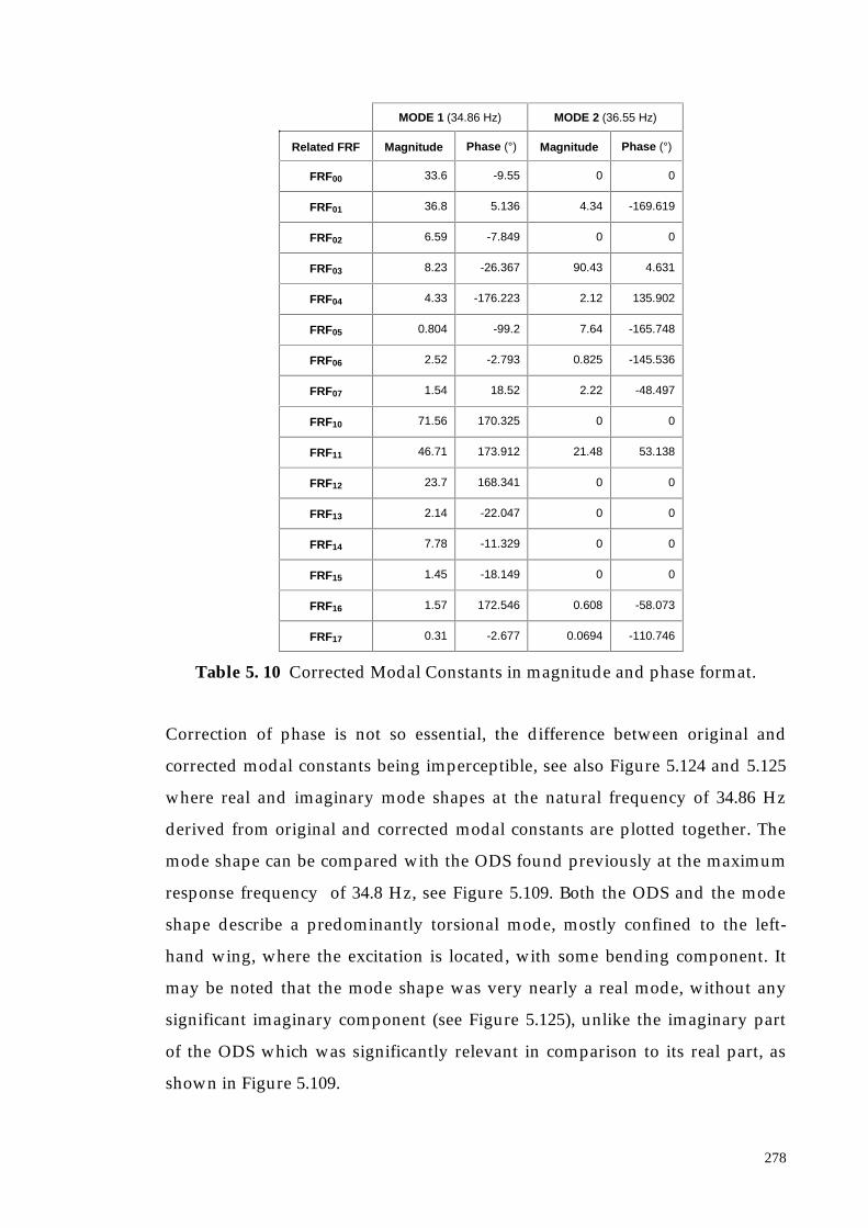
278

MODE 1 (34.86 Hz) MODE 2 (36.55 Hz)

Related FRF Magnitude Phase (°) Magnitude Phase (°)

FRF00 33.6 -9.55 0 0

FRF01 36.8 5.136 4.34 -169.619

FRF02 6.59 -7.849 0 0

FRF03 8.23 -26.367 90.43 4.631

FRF04 4.33 -176.223 2.12 135.902

FRF05 0.804 -99.2 7.64 -165.748

FRF06 2.52 -2.793 0.825 -145.536

FRF07 1.54 18.52 2.22 -48.497

FRF10 71.56 170.325 0 0

FRF11 46.71 173.912 21.48 53.138

FRF12 23.7 168.341 0 0

FRF13 2.14 -22.047 0 0

FRF14 7.78 -11.329 0 0

FRF15 1.45 -18.149 0 0

FRF16 1.57 172.546 0.608 -58.073

FRF17 0.31 -2.677 0.0694 -110.746

Table 5. 10 Corrected Modal Constants in magnitude and phase format.

Correction of phase is not so essential, the difference between original and

corrected modal constants being imperceptible, see also Figure 5.124 and 5.125

where real and imaginary mode shapes at the natural frequency of 34.86 Hz

derived from original and corrected modal constants are plotted together. The

mode shape can be compared with the ODS found previously at the maximum

response frequency of 34.8 Hz, see Figure 5.109. Both the ODS and the mode

shape describe a predominantly torsional mode, mostly confined to the left-

hand wing, where the excitation is located, with some bending component. It

may be noted that the mode shape was very nearly a real mode, without any

significant imaginary component (see Figure 5.125), unlike the imaginary part

of the ODS which was significantly relevant in comparison to its real part, as


279

Figure 5. 124 Real part of the mode shape at the natural frequency of 34.86 Hz

derived from original (left) and corrected (right) modal

constants.

Figure 5. 125 Imaginary part of the mode shape at the natural frequency of

34.86 Hz derived from original (left) and corrected (right) modal

constants.

A “hybrid” correlation between the ODS ( [ODS] ) at the measured resonance

frequency of 34.8 Hz (Figure 5.109) and the mode shape ( [MODE] ) derived via

modal analysis at the natural frequency of 34.86 Hz (Figure 5.124) can be done

[1] using the mode-response correlation parameter (MFAC) defined by the

following equation:

280

[ ] [ ]( )

=

∑∑∑∑

∑∑

= == =

= =

n

i

m

jjiji

n

iji

m

jji

n

i

m

jjiji

MODEMODEODSODS

MODEODS

MFAC

1 1

*

1

*

1

2

1 1

*

, MODEODS (5. 86)

where n is the number of DOFs in the x-direction and m is the number of DOFs

in the y-direction. Therefore, if the ODS and the mode shape are plotted for x = -

1..0.02..1 and y = -1..0.02..1, it will be n = m= 101. The degree of correlation

(MFAC) between the operating deflection shape and the mode shape was 73.34

%.

Figure 5.126 shows real and imaginary components of the mode shape for the

natural frequency of 36.55 Hz (corrected modal constants are used), while

Figure 5.127 reports, for completeness, the ODS derived by the conventional

continuous area scan performed at only one frequency, that of the maximum

response, which was found at 36.6 Hz. Both the ODS and mode-shape

corresponded to a real bending mode, largely uncontaminated by torsional

motion.

Figure 5. 126 Real (left) and imaginary (right) part of the mode shape at the

natural frequency of 36.55 Hz derived from corrected modal

constants.

281

Figure 5. 127 Real and imaginary ODS at 36.6 Hz.

5.6.3 Concluding Remarks

In this last section, an unusual modal analysis performed on continuous area

scan data obtained by conventional step-sine test experimental procedure has

been described. In the end, it was shown that the modal analysis procedure can

be used also in the standard way the correction needed, giving no remarkable

difference.

The ODSs derived by continuous area scanning are generally complex, as there

is a significant out-of-phase component in the dynamic deflected form. In

general, the shape of the ODS, even at a natural frequency, depends to some

extent on the position of the applied excitation, whereas the natural mode-

shape does not. The ODS is complex because it is a combination of the mode

shapes occurring at frequencies close to that of the excitation. It is then affected

by the off-resonant contributions from the other modes. Natural mode shapes

must therefore be derived from ODSs by modal analysis by performing a step-

sine test, i.e. by extracting modal characteristics from frequency response

functions (response / force ratio) data, measured at a succession of frequencies

spaced suitably around the natural mode being analysed. In this context, the

force input had to be quantified; it must therefore be acquired via a force cell

282

attached on the structure at the shaker position and sampled simultaneously

with the LDV signal. Both signals are then subjected to the same post-

processing: the force input recorded is multiplied by sine and cosine functions

at the excitation frequency (ω) to determine magnitude and phase. FRFs are

then derived by complex division and they are assembled together in order to

have an FRF for each CSLDV sideband spectral component. The end result of a

modal analysis of these FRFs is a rather novel eigenvector, not of individual

point responses, but of polynomial coefficients representing the responses of

the complete ensemble of points contained within the scanned area.

It must be emphasised that with the CSLDV area sine scan, modal analysis need

only be applied to the polynomial coefficient data (or, indeed, to the averaged

sideband data, before applying the transform to recover polynomial

coefficients). The number of FRFs to be analysed is thus smaller than the

number of FRFs that have to be taken into consideration when a point-by-point

area scan is performed. The latter process is computationally intensive because

of the large number of spatial positions to be addressed. The time saving on the

analysis must be added to the saving on the acquisition time, as already stated

in this Chapter. With the CSLDV technique used for modal analysis step-sine

tests must be carried out. At each step-frequency excitation, only one

acquisition has to be made. If the slower scan speed is of, say, 0.3 Hz, the

acquisition time will be at least 3.33 secs, in order to cover the whole tested

surface. The overall acquisition time (for a complete step-sine test) will be a

number of times longer than the single-step acquisition time corresponding to

the number of frequency-steps which are required. However, this time will be

shorter than the time required to acquire the FRFs at all points defined in the

discrete scanning technique.

Finally, it should be pointed out that the final resolution of the mode shape as it

is plotted out is completely independent from the acquisition. While the spatial

resolution of a mode shape derived from FRFs measured by using a point-by-

point scan is represented by the number of points measured, the spatial

283

resolution of the mode shape obtained from CSLDV FRFs data is totally

arbitrary. In fact, the mode shape is represented by a polynomial whose

coefficients are derived from the post-processing of the measurement data.

With these coefficients the polynomial can be plotted over whatever grid of

points is required, i.e. with any resolution one choses. For example, in the plots

of Figures 5.126, 5.127, 5.128 and 5.129 a resolution of 101 × 101 points was

used.

5.7. Conclusions

This chapter has covered a number of applications of a continuous-scan LDV to

the measurement of response mode shapes (ODSs) using line (straight and

circular lines) and area scanning. Single-frequency vibration, as produced with

sinusoidal vibration of a linear structure, is assumed. Two basic methods of

signal processing are described: (i) demodulation and (ii) sideband

identification. The first of these will give an ODS with the resolution of the

signal sampling, and to the accuracy of the basic LDV measurement. The

second method produces a representation of the ODS in a polynomial series

form. If the ODS is a smooth function of position, without discontinuities,

higher terms in the series become insignificant, and the ODS may be

represented with little error by a relatively small number of series coefficients.

The continuous scan demodulation technique does not require, instead, that the

mode shape is smooth within the scanned area. This approach can then be used

on structures with discontinuities on the surface, i.e. apertures or corrugations.

The disadvantage of this technique is that it is sensitive to the speckle noise

which may limit its accuracy locally. Linear circular scans and circular area

scans have been applied to disc-like structures in order to recover

circumferential and 2-D mode shapes of the disc respectively.

For all these techniques, mathematical analysis has been performed, and then,

they have been shown to work effectively by performing omparisons with

experimental data measured on simple structures as beams, plates and discs.

284

For some methods (such as sinusoidal straight line scan and sinusoidal

rectangular area scan), further analysis have been made by measuring the

corresponding ODSs via the Polytec system applied in its conventional fashion

(single point scan).

In the last section a procedure to recover mode shapes from data measured by

the area scanning technique has been illustrated. Scanning LDV ODS

coefficients may easily be repeated in a frequency-step sequence and converted

into FRF form, so that modal analysis can be applied to extract modal constants.

The method has been applied to a practical test specimen, i.e. the GARTEUR

structure, in order to make the procedure clearer and easier to be followed.

Chapter 6 Virtual Testing

6.1. Introduction

The continuous scanning LDV technology, described and tested in all its facets

in the previous chapters, is studied here from a different perspective. The aim

of this part of the work is to simulate the experimental procedure which must

carried out when a CSLDV measurement has to be performed. This technique,

when applied to practical case studies, needs to be performed by specialists

skilled in the LDV field, otherwise the setting-up process could become

extremely time-consuming. The rehearsal of all the steps accomplished in the

laboratory during a CLSDV experiment can be done via a numerical simulation

which is called a “virtual test”. This process can be useful as a means (i) to

optimise the actual test by selection of the best experimental parameters, a

priori, and (ii) to train engineers on the fairly new continuous scanning

philosophy.

286

6.2. Virtual Testing Technique

Virtual testing is a new technique devised in order to make the actual tests

more effective and less time-consuming, and thus to reduce their cost. In fact,

nowadays experimental structures tend to be overbooked and the length of

time which they can spend in a laboratory is limited.

In order to carry out a virtual test, a mathematical model of the whole test

structure and set-up must be developed where a model of the dynamic

properties of each element in the test set-up must be included. Such a model

will simulate the input signals actually used in the real test, including the

sources of noise as and where they are experienced by the acquisition sensors in

real measurements. In these conditions, the derived response functions can be

supposed to well reproduce the real data which would be measured by

performing a true test.

The concept of virtual testing can be applied to continuous scanning laser

Doppler vibrometry treated in this work in order to investigate ahead of time

the applicability and the accuracy of the various techniques which depend on

the conditions in which the system operates.

The simulation of a continuous scanning test is based on the application of the

algorithms illustrated in detail in Chapters 4 and 5 for the different techniques

by using numerical data rather than (or before) actual measured data.

Parameters describing the operating conditions of the test are introduced into

the numerical model of the measurement system in order to verify their effects

and to allow forecasting the best settings of these parameters. The optimum test

configuration and design can then be decided a priori before entering the

laboratory.

The computer model of the structure under test will act as a realistic simulator

that can yield computed LDV responses containing the various “errors” that

287

have been found to contaminate the data measured in real tests. The most

important practical deviation from an ideal measurement by an LDV is due to

the speckle noise to which the LDV is intrinsically sensitive. The speckle noise

depends on interfering inputs of a random nature mostly related with the

characteristics of the tested surface: it can actually be considered as a

measurement of the roughness of the surface itself and as such cannot be

avoided. It is important then to determine the reasons for the occurrence of this

phenomenon (see Chapter 2) which distorts the LDV output signal, and thence

the experimental parameter settings that can be manipulated in order to

provide a prediction version of the optimal working conditions. This approach

greatly improves the chances for a successful test and saves, simultaneously,

time in “tuning” the experimental process.

The speckle noise effect will be treated briefly in next section, the subject having

already been discussed in detail in Chapter 2. First, the occurrence of the

speckle noise in a traditional single point LDV used for step-scanning over

discrete points will be mentioned, and then its presence in a continuous

scanning LDV operation will be considered. A mathematical model of the noise

superimposed on the ideal signal will be developed in order to simulate the

vagaries of real test data and to predict realistic LDV responses when the laser

beam moves continuously over the test structure. In this software model a

specific parameter is introduced which identifies the actual continuous

scanning test adopted and which is the scan speed of the moving laser beam. In

this way the optimal scan rate that should be employed to drive the scanning

system can be decided a priori.

6.3. Mathematical Model

The mathematical model of an experiment performed with an LDV system used

in the continuous scan fashion will consist mainly of the algorithm described in

Chapter 5 and employed to test analytically the post-processing techniques

288

used to recover ODSs from the simulated time histories. For instance, some

previous simulations can be recalled:

(i) Equation (5.6), which produces a simulated LDV output when uniform

straight-line scan is performed. A typical time signal is shown in Figure

5.3;

(ii) Equation (5.27), used to predict the time history which could be acquired

by the vibrometer if the laser beam is scanning sinusoidally along a

straight-line. Scanning mirror delays are also taken into account here.

Figure 5.19 illustrates the time signal obtained; and

(iii) Equation (5.63), which simulates the LDV output in the time domain

considering the laser scanning over a 2-D area (area scan) and including

in the algorithm the mirror driver delay. For the simulated time signal

see Figure 5.69 (bottom plot).

In order to complete the mathematical model to make a simulated velocity

signal look like an experimental signal, the noise affecting real test data must be

modeled as well. When an LDV system is used for measurement, the main

source of pollution is the speckle noise or, in other words, the speckle noise

prevails over all the other kinds of random noise. In the following section, a

model for the speckle noise will be developed.

As already stated (see Section 2.4), speckle noise occurs when monochromatic,

coherent light, scattered from an optically rough surface, is collected by a

photodetector. In the detector’s collecting surface a speckle pattern is formed. If

the speckle pattern undergoes spatial and temporal changes these latter will

modulate the Doppler signal which is the output from the photodetector. Such

kind of changes are caused by target motions as tilt or in-plane translation, that

produce a Doppler signal phase modulation, referred to as speckle noise.

For fixed-point measurements, in particular if there is a large vibratory

displacement perpendicular to the LDV beam, speckle can cause severe

problems because the speckle noise can become synchronous with the

289

vibration, leading to severe harmonic distortion. In fact, speckle noise is noted

at certain points in the spatial field of the velocity information measured by the

LDV. It appears as occasional velocity drop-outs which are unidirectional,

always estimating velocity response closer to zero than reality. The areas of

drop-out translate the data points of the velocity response into data points

which are closer to the zero axis for both positive and negative velocities. Thus,

the laser noise can be classified as a “biased-low” due to the fact that the drop-

out effects in the velocity signal produce absolute velocity data which are lower

than similar velocity signals which do not contain drop-out.

The drop-out areas have been seen to occur more predominantly at points of

minimum linear velocity response with big local tilt components (“nodes” of

the structure), see reference [29].

The occurrence of the speckle noise can be explained by the fact that during

vibration the point illuminated by the laser is not identical through the entire

period of motion, [4]. This results in the detector receiving a changing speckle

pattern over the course of the periodic motion of the structure. When the

speckle covered by the detector is “dark” or is “bright”, but it scatters back

towards the detector an insufficient intensity of light, the Doppler signal

amplitude falls below the threshold of the demodulator circuit used to derive

the analogue velocity waveform from the Doppler signal and velocity drop-outs

are yield.

Since the noise appears at specific areas (vibrational node) its effect is

commonly reduced either by averaging or by statistically smoothing the

measured data. These methods have the disadvantage that they bias the data

averaged because the speckle noise always appears as a drop towards zero of

the velocity signal.

When the measuring laser beam is not steady over the surface to be measured,

but scans continuously, and, for instance, it moves backward and forward

along a straight-line a relative motion between structure and laser occurs. The

speckle noise will then appear since the photodetector collecting the light

scattered by the target surface experiences also the motion of the “dark” and

290

“light” speckles. The output signal will contain drop-outs when a “dark”

speckle grain is encountered. The presence of “dark” or “light” speckles along

the light is random since they depend on the light-scattering properties of the

surface, i.e. on the surface roughness. But, if the laser beam travels along the

same line all the time, then it meets always the same succession of “light” and

“dark” speckles, and the photodetector will notice the same spatial distribution

of speckle grains in each scan cycle. The noise effect will appear periodic with

the laser scan frequency since in each scan cycle it will be located at the same

phase value. The speckle noise can be seen, as the experimental data will

demonstrate (see subsection 6.4.3), as it concentrates all its content at some

frequencies which are, namely, the scan frequency and its harmonics. These

harmonic frequencies, which constitute a sort of noise floor, are due to a so-

called “pseudo-vibration”, [50], because it is introduced by the laser motion.

They should not coincide with the genuine vibration frequency and any

relevant sideband frequencies otherwise their level, even low, will pollute the

true vibration information. It is therefore essential that the scan speed is chosen

carefully in order to be sure that none of its harmonics will overlap with the

structural vibration frequency and its sidebands.

Consequently it can be deduced that the scan frequency becomes an important

parameter which should be controlled in order to have the best measurement

data (best SNR, since it is possible directly to interfere on the noise content of

the LDV output).

6.4. Speckle Model

6.4.1 Introduction

The aim of this section is to present a model of the velocity signal measured by

an LDV sensor which is continuously scanning over the target surface, taking

into account the luminous intensity variation due to the random shifts caused

291

by the motion of the speckle pattern that is incident on the instrument’s

photodetector. In fact, the Doppler signal coming from the LDV is modulated

by the changes of the speckle pattern formed by the light scattered back from

the surface illuminated by the laser beam. Certain types of motion of the tested

surface, such as rotation (see reference [45]) or in-plane motion (see reference

[46]), produce spatial and temporal modifications of the speckle pattern and

lead to a Doppler signal phase modulation clearly seen in the LDV output. In

practice, since the speckle grains vary their spatial distribution, the

photodetector will experience this motion as a shift in frequency similar to the

shift due to the Doppler effect in which the information to be measured exists.

The phenomenon commonly referred as “speckle noise” will produce an

uncertainty in the derivation of the vibration response from the Doppler signal

in output from the LDV. In the case with which this work deals, an in-plane

relative motion can be still considered with the only difference that, now, the

system which moves is not the target but the measurement laser beam. Since

the laser beam travels sinusoidally around in circles or backwards and forwards

along lines, its motion is periodic with a frequency which is the scan speed. This

means that the speckle changes are periodic as well and their frequency content

is concentrated at the fundamental motion frequency (the scan frequency) and

its harmonics. For instance, if the laser beam travels along a line on the

measured surface at a frequency of 10 Hz, the LDV output spectrum will show

peaks at 10 Hz and its harmonics, also if the structure is not vibrating at all. It is

possible to state, then, that there exists a “pseudo-vibration” due to the laser

motion, and therefore due to the speckle pattern motion, which is

indistinguishable from the genuine vibration. In order to reduce its importance,

the speckle noise amplitude must be minimised otherwise it must be assured

that its frequency content does not coincide with the vibration frequency and its

sidebands. A theoretical model of the speckle noise has been developed in order

to simulate the distortion that will be produced on the LDV output when the

speckle pattern undergoes an in-plane motion and a validation of the model has

been performed by comparing theoretical results with experimental data.

292

6.4.2 Theoretical Model of the Light Intensity Collected by the Photodetector

First, an analytical representation of the light intensity received at the

photodetector can be derived by recalling the formulae established in Section

2.8, Equations (2.80). In order to consider the speckle pattern motion, phase

information should be included in the light intensity formulation. Writing the

electric field associated to the reference beam as E1 and A1 and θ1 its amplitude

and phase, respectively, and E2i the electric field associated to the measuring

beam scattered back from the ith speckle grain (A2i, and θ2i, are the amplitude

and the phase of E2i), Equations (2.80) will become:

( )[ ] ( )[ ] iDii

S

tffiAE

tffiAE

222

111

2exp

2exp

θπθπ+−=

++=(6. 1 )

where f is the frequency of the laser source employed, fS is the frequency shift

induced in the reference beam by the Bragg cell and fD is the Doppler frequency

carrying the velocity information required. The resultant intensity scattered by

the ith speckle and observed by the photodector, Ii, can be derived by the

combination of the two beams intensities:

[ ][ ] ( ) ( )[ ] ( )

−++++=

=−++++=++=

iSiii

iDSiiiiiii

tvtIIIIKS

tffAAAAKSEEEEKSI

212121

212122

21

*2121

4cos2

2cos2

θθλπω

θθπ

(6. 2)

ωS being the reference beam angular frequency shift, vλπ2

the Doppler

frequency, fD, (with λ the laser source wavelength and v the target velocity) and

K the constant radiant sensitivity of the active area, Si, on the photodetector

which receives the light scatterd from the ith speckle.

293

The first component (I1 + I2i ), also named intensity noise, is at a relatively low

frequency and is often constant (DC), as it usually occurs in experimental tests,

so it can be filtered out to leave the LDV output to represent the Doppler signal

only:

( )

−+−= iSiii tvtIIKSI 2121

4cos2 θθ

λπω (6. 3)

If the active area on the photodetector is now considered, the area where the

light intensities scattered from n speckle grains arrive, the total current

generated by the detector will be:

++==∑

=TOTSTOT

n

ii tvtKIII Θ

λπω 4

cos1

(6. 4)

From Equation (6.4) the angular beat frequency produced by the heterodyne

process between the reference and the measuring beams, involved in the

measurement in the LDV system, can be derived as:

dt

dv TOT

S

Θ++=λπωω 4

(6. 5)

Two cases can be then underlined:

(i) if the n speckle grains scattering the light towards the photodetector

have constant phase, which happens when the speckle pattern does not

undergo any spatial changes, the output spectrum of the LDV will

contain peaks at the vibration frequency only, the term dt

d TOTΘ being

zero. This case occurs if any in-plane motion is imposed on the target

structure.

294

(ii) if the speckle pattern experiences changes in its spatial and temporal

characteristics (i.e. speckle “boiling” or/and “translation” occur ,see

Section 2.4), the derivative dt

d TOTΘ becomes non-zero and it will be the

term related to the speckle noise which can be seen in the LDV output.

The spectrum of this latter will still contain the peaks at the vibration

frequencies but noise will be superimposed at frequencies corresponding

to the spectral content of dt

d TOTΘ.

The second case occurs when a continuous scanning LDV technique is used.

The speckle pattern will evolve in sympathy with the target motion, in this case

with the relative movement between the target and the laser beam (here, it is

the laser beam which actually moves). In this situation, where the laser beam

scans continuously along a straght line, it can be assumed that the dominant

motion which the speckle pattern undergoes is translation and, specifically, that

it is a periodic translation following the motion of the laser beam. If the latter

moves sinusoidally backwards and forwards along a straight line, the speckle

grains will translate across the detector active area with the same frequency as

the scanning beam motion. Figure 6.1 shows the spectral components of the

simulated light intensity that would be recorded by the photodetector in both

cases where the speckle phase fluctuation is zero and non-zero (left and right

plots, respectively). The left-hand plot has been derived from Equation 6.4 for a

beat frequency of approximately 403 MHz, considering a Bragg frequency shift

of 40 MHz (ωS), a He-Ne laser source with wavelength of 633 nm (λ) and a

vibration velocity occurring at a frequency of 115 Hz. On the other hand, the

right-hand plot has been obtained for the situation when the measuring laser

beam is continuously scanning along a line at a speed of ΩL (say10 Hz). The

speckle grains will then undergo a periodic motion with a periodicity of 10 Hz.

If we introduce a simplified1 model where it is assumed that the phase of the

speckle pattern changes periodically as:

1 In practice, the change of the speckle pattern phase is a periodogram at the scan frequency and higherorder harmonics and it can be modeled as amplitude modulated comb function. Equation 6.6 is adoptedfor simplicity purpose.

295

( )tLTOT ΩΘ sin= (6. 6)

and then its derivative will become non-zero.

The light intensity collected by the photodetector will then have a spectral

content described by:

( )tv LLS ΩΩ cos4 ++=λπωω (6. 7)

which means that the intensity appears as a frequency-modulated signal and its

spectrum will contain sidebands at ± ΩL centered at the frequency of 403

MHz.

Figure 6. 1 Simulated light intensity collected at the photodetector (which is

sensitive to current signals, i.e. Ampere) for phase fluctuation zero

(left) and non-zero (right).

In practice, when an LDV is employed for experiments, the instrument output

is an analogue voltage derived by demodulating the Doppler signal represented

by the light intensity collected at the photodetector. The voltage output

represents the target vibration velocity directly. As it has been already outlined

Frequency (Hz)

Am

pli

tud

e (A

)

403 MHz

Frequency (Hz)

Am

pli

tud

e (A

)

403 MHz ± 10 Hz

296

(see Section 6.3), when a continuous scan is performed by using a scanning

LDV the output spectrum contains the characteristic speckle noise peaks at the

scan frequency and its harmonics.

6.4.3 Experimental Speckle Noise Analysis

Before building a mathematical model which can reproduce the noise due to the

speckle pattern displacement when a relative motion between surface to be

measured and laser spot on the surface itself occurs (laser beam scanning

continuously along the surface), an analysis of experimental data acquired in a

real test has been performed. The analysis has been done on a structure used for

a practical application where the noise analysis was needed before starting the

real experimental work in order to derive the optimal scan speed which would

allow us to have the best measurement data (higher SNR) The structure

consisted of the rear panel of a lorry cab which was a case study within the

BRITE/EURAM project VALSE, [13]. The analysis took into account two

parameters that were thought to influence the speckle noise behaviour: (i) the

laser beam scan speed and (ii) the scan length of the line traveled by the laser

beam. By varying these parameters, the speckle noise experienced by the LDV

sensor was studied.

The tested structure was the rear panel of an IVECO DAILY motor lorry cab,

see Figure 6.2, where the continuous scanning techniques (specifically, long

scan along a line) were applied in order to prove their proper functionality also

in complex structures.

297

Figure 6. 2 Experimental structure.

Before commencing the continuous-scan measurements, the opportunity was

taken to assess the LDV noise at different scan rates and different scan lengths.

First, different LDV output time histories were acquired at different scan speeds

(i.e. at 0.2, 0.5, 1, 5, 10, 20 Hz) along a vertical line 740 mm long, on the lorry cab

back panel, without exciting the panel. Two sets of measurements were

recorded: one driving the mirror with a sine wave and the other with a

triangular wave. Observing the FFTs of those signals for the sinusoidal scans

(Figure 6.3), it is noticeable that the noise increases with the scan speed and is

concentrated at the scan frequency and its harmonics. Figure 6.3 also shows

zoomed LDV output spectra to highlight that there is a broad-band noise-floor,

which also increases with scan rate. Note that in the left-hand plot of Figure 6.3

only the LDV spectra at 1, 5, 10, 20 Hz are reported in order to have a more

legible figure. However, the spectra at 0.2 and 0.5 Hz have such a low noise

content that they can be neglected.

SCANLINE

298

Figure 6. 3 Measured LDV output spectrum, case of laser beam scanningsinusoidally.

The amplitude of the LDV spectrum component at the scan frequency increased

with the scan speed, as shown in the left-hand plot of Figure 6.4. The noise floor

amplitude, which is defined as the maximum amplitude of the LDV output

spectrum, the peak at the scan frequency being excluded, is shown in the right-

hand plot.

Figure 6. 4 Noise, plotted against the scan frequency – sinusoidal scan.

0 20 40 60 80 100 120 140 160 180 2000

0.1

0.2

0.3

0.4

0.5

0.6

0.7

0.8

0.9

Frequency (Hz)

LDV

out

put

(V)

Scan Speed 20 HzScan Speed 10 HzScan Speed 5 Hz Scan Speed 1 Hz

0 5 10 15 20 25 300

0.01

0.02

0.03

0.04

0.05

0.06

0.07

0.08

0.09

0.1

Frequency (Hz)

LDV

out

put

(V)

Scan Speed 20 Hz Scan Speed 10 Hz Scan Speed 5 Hz Scan Speed 1 Hz Scan Speed 0.5 HzScan Speed 0.2 Hz

0 2 4 6 8 10 12 14 16 18 200

0.1

0.2

0.3

0.4

0.5

0.6

0.7

0.8

Scan Frequency (Hz)

Flo

or N

oise

leve

l (V

)

0 2 4 6 8 10 12 14 16 18 200

0.1

0.2

0.3

0.4

0.5

0.6

0.7

0.8

Scan Frequency (Hz)

FF

T a

mpl

itude

(V

) at

the

Sca

n F

requ

ency

com

pone

nt

299

In the second case, the mirror was driven by a triangular wave, i.e. scan at

uniform rate (see in Figure 6.5 the LDV output spectra): the noise behaviour

(Figure 6.6) is the same, the only difference being that it is a bit smaller -

specifically 25 % less. This value was derived from the maximum noise level in

both cases - sinusoidal (0.8317 V at 20 Hz) and uniform scan (0.6202 V at 20 Hz).

Again, as in Figure 6.3, in the left-hand plot of Figure 6.5 the spectra at 0.2 and

0.5 Hz are not reported.

Figure 6. 5 Measured LDV spectrum, case of laser beam scanning at uniformrate.

The noise behaviour is displayed in Figure 6.6 and, since the laser beam was

scanning at uniform rate, it was plotted against the scan speed in m/s.

Figure 6. 6 Noise, plotted against scan speed – scan at uniform rate.

0 20 40 60 80 100 120 140 160 180 2000

0.1

0.2

0.3

0.4

0.5

0.6

Frequency (Hz)

LDV

out

put

(V)

Scan Speed 20 HzScan Speed 10 HzScan Speed 5 Hz Scan Speed 1 Hz

0 5 10 15 20 25 300

0.01

0.02

0.03

0.04

0.05

0.06

0.07

0.08

0.09

0.1

Frequency (Hz)

LDV

out

put

(V)

Scan Speed 20 Hz Scan Speed 10 Hz Scan Speed 5 Hz Scan Speed 1 Hz Scan Speed 0.5 HzScan Speed 0.2 Hz

0 5 10 15 20 25 300

0.1

0.2

0.3

0.4

0.5

0.6

Scan Speed (m/s)

Flo

or N

oise

leve

l (V

)

0 5 10 15 20 25 300

0.1

0.2

0.3

0.4

0.5

0.6

Scan Speed (m/s)

FF

T a

mpl

itude

(V

) at

the

Sca

n F

requ

ency

com

pone

nt

300

These data were used to select suitable scan rates for the continuous-scan

measurements.

By this noise analysis it was demonstrated that the scan speed is the most

influential parameter on the noise behaviour. It was then deduced that the

speckle model should be built on the basis of this parameter since, when

varying the scan speed, the noise occurrence change consequently. The noise

will appear at the scan frequency and its harmonics and its level will increase as

the scan frequency increases. Therefore, when a continuous scanning LDV is

employed, the laser beam scan speed will be chosen as a compromise: (i) it

should be high (from 10 up to 20 Hz) so that, the noise being concentrated in its

harmonics only, the presence of the noise itself will be limited and (ii) the scan

frequency and all its harmonics must no coincide with the excitation frequency

and its sidebands otherwise the derived response will be spoilt with the noise

and cannot be reliable anymore. By arranging the scan speed in relation to the

vibration frequency, the frequency range of interest, which includes the

vibration response frequency with its sidebands, can be made to lie far apart

from the scan speed harmonics. The spectral components used in the curve-fit

analysis will then be unspoiled by the noise.

After the analysis at different scan speeds was completed, several LDV output

acquisitions were performed by changing the scan length, which was taken at

four values:

(i) 20 mm,

(ii) 30 mm,

(iii) 170 mm, and

(iv) 300 mm.

Figure 6.7 shows the amplitude of the noise level at 20 Hz and its harmonics for

all the situations at different scan lengths. It can be noticed that the speckle

noise is concentrated mostly at 20 Hz, where it increases as the scan length

increases. On the other hand, at the higher harmonics the noise level decreases

301

no matter what scan length is used. This means that the noise assumes

importance at the scan frequency only and this does not constitute a big

problem since the scan frequency can always be made to be smaller than the

vibration frequency. Therefore the noise does not necessarily pollute the

information required (i.e. the vibration response) from the measured data.

Figure 6.8 is a different, more compact, visualisation of the speckle noise

contents at the different scan length and scan frequency harmonics. It can be

seen, again, that its level is maximum at the scan frequency whatever the scan

length is, but this value increases with the scan length. The noise content at the

upper harmonics is always small. For a long scan the reduction is more

noticeable than for small scans, see Table 6.1 for a quantitative representation of

this reduction.

50 100 150 200 250 300 350 400 450 5000

0.02

0.04

0.06

0.08

0.1

0.12

0.14

0.16

0.18

Harmonics Frequency (Hz)

LDV

spe

ctra

l am

plitu

de (

V)

Scan Length 30 cmScan Length 17 cmScan Length 30 mmScan Length 20 mm

20

Figure 6. 7 Speckle noise level plotted against the scan frequency and its

harmonics for the different scan length.

Table 6.1 reports the difference between the noise level occurring at the scan

frequency (20 Hz) and the noise level at the higher harmonics. This difference,

called “noise reduction”, is obtained for each scan length by subtracting from

the noise level at 20 Hz the averaged noise amplitude at all the higher

harmonics and it is given as a percentage of the noise level at 20 Hz.

302

Scan Length (m) Noise Reduction (%)

0.02 81.49

0.03 74.58

0.17 80.43

0.30 91.96

Table 6. 1 Noise reduction at high-frequency range.

Figure 6.8 shows the noise content at the different harmonics of 20 Hz (i.e. the

scan speed) and at the different scan lengths between 0.02 and 0.3 m.

Figure 6.8 Color-map of the speckle noise level simultaneously plotted against

the scan length and the scan frequency and its harmonics.

From the experiment results described in this section, it can be noted that the

noise at higher harmonics of 20 Hz is smaller by around 80-90 % with respect to

the noise level at 20 Hz and it can be neglected. The scan length consequently

influences the noise content at the scan frequency only and, as was already

highlighted, the scan frequency component does not assume big importance

within the complete LDV output spectrum. In fact, the information required,

303

namely the vibration response, is at the vibration frequency which is usually

much higher than the scan frequency. It can thus be concluded that the scan

length does not affect the quality of the measured data and it will not be

included in the speckle noise model, which will take into account the scan

speed only.

6.4.4 Simulated Speckle Noise

If a measuring laser beam moving continuously along a line on a structure is

considered, it must be clear that the speckle pattern seen by the laser would

change since the surface swept is changing. The speckle noise characteristic that

the experimental analysis has shown, i.e. the classical noise concentration at a

scan frequency and higher harmonics, can be explained with regard to a simple

model. It will be assumed that the laser beam scans sinusoidally at the speed of

10 Hz backwards and forwards along a straight-line and over this line all the

speckles swept by the laser are “bright” with the exception of one, which is

“dark”. When the laser beam passes through this speckle, the light scattered

back towards the photodetector will experience a drop-out. The LDV output

will then present a loss of the signal twice within a scan cycle since the laser is

going backwards and forwards along the scan line. The LDV output and its

spectral content are illustrated in Figure 6.9.

Figure 6.9 Simulated LDV output time signal showing drop-outs and

corresponding Fourier spectrum.

0 0.1 0.2 0.3 0.4 0.5 0.6 0.7 0.8 0.9 1Time (s)

LDV

out

put

(V)

0 50 100 150 200 250 300 350 400 450 5000

0.02

0.04

0.06

0.08

0.1

0.12

0.14

0.16

0.18

0.2

Frequency (Hz)

LDV

Spe

ctra

l am

plitu

de (

V)

304

A model of the speckle noise can then be developed on the basis of the

considerations derived from the experimental analysis that can be summarised

as:

(i) speckle noise is concentrated at the scan frequency and its harmonics,

and

(ii) the speckle noise at the scan frequency occurs with a higher level.

The model can be then written as:

( ) ( ) ( )

Ω+Ω= ∑

=Ω

harmofn

nLLatSPECKLE tnnvbtAphasespeckleofchangeofrate

L

.

2

2cos2cos ππ

(6. 8)

ΩL being the scan frequency of the measuring laser beam, v a normalised

random variable which represents the amplitude of the LDV spectrum at the

harmonics of the scan frequency, n is an integer which it depends on the

number of harmonics of the scan frequency that it is decided to be included,

ASPECKLE at Ω is the amplitude of the speckle noise at the scan frequency and b is a

parameter which links the noise level at the scan frequency with the noise level

at its harmonics (see the following analysis).

From the experimental noise analysis it is possible to deduce how the noise

level occurring at scan frequency of the measuring laser beam and at its

harmonics is related to the scan frequency itself.

First, it should be pointed out that the noise level at higher harmonics is always

smaller than the noise amplitude at the scan frequency, as Table 6.2 shows. The

“noise reduction“ is calculated as a percentage difference between the noise

level at the scan frequency and the maximum noise level at the higher

harmonics.

305

Scan Frequency(Hz)

Noise level at theScan Frequency

(V)

Maximum Noise level atthe Higher Harmonics

(V)

Noise Reduction(%)

0.2 0.0072 0.0049 32.41

0.5 0.0182 0.0058 68.13

1 0.0371 0.0105 71.62

5 0.1600 0.0393 75.43

10 0.3200 0.0800 75.00

20 0.8400 0.2600 69.05

Table 6. 2 Noise amplitude at the scan frequency and at high-frequency

harmonics, and relative reduction.

With the exception of a scan rate of 0.2 Hz, where the noise level at the scan

frequency itself is very low, the difference between the noise amplitude at the

scan frequency and that at the higher harmonics can be assessed around 72 %,

(“noise reduction”, from the third column of Table 6.2). It can be deduced then

that the parameter b appearing in Equation (6.8) will assume a value of about

0.28.

Moreover, from the experimental noise analysis, and specifically from the

graphic shown in the right-hand plot in Figure 6.4, a relationship between the

scan frequency and the noise level at the scan frequency can be deduced. It can

be noticed that the noise amplitude increases with the scan speed with a linear

behaviour up to 10 Hz then a big rise occurs up to 20 Hz, see right-hand plot in

Figure 6.4. The noise data plotted in this graph can be curve-fitted by a

polynomial of the third degree, which can be written as:

322335 11.157.317.134.7 −−−− ++−= eeeeA LLLatSPECKLE LΩΩΩΩ (6. 9)

Figure 6.10 shows the matching of this polynomial relationship with the

measured data plotted in Figure 6.4 (right-hand plot).

306

0 2 4 6 8 10 12 14 16 18 200

0.1

0.2

0.3

0.4

0.5

0.6

0.7

0.8

0.9

Scan Frequency (Hz)

Noi

se a

mpl

itude

(V

)

Figure 6. 10 Measured noise level data (black dots) and their polynomial curve-

fit (blue line).

Equations (6.8) and (6.9) can be used to build a speckle noise model.

The LDV output obtained by a measurement performed by a laser beam

moving continuously at 10 Hz along a straight-line can be simulated, by using

Equation (6.8) by setting ΩL = 10 Hz, n. of harmonics = 100, b = 0.28 , and

3138.0=LatSPECJKLEA Ω V, derived from Equation (6.9) for ΩL = 10 Hz.

Some random noise, related to different types of ‘error’ inevitably contained in

the real test data, is added to the model of the speckle noise as well.

The results are shown in Figure 6.11 where the left-hand plot shows the

simulated time signal, which the model produced as LDV output, while the

right-hand plot illustrates the real data measured in time domain (the measured

time history is taken from the experiments described in Subsection 6.4.3,

specifically for a scan speed of the laser beam of 10 Hz). In Figure 6.12 the

relative LDV spectra are depicted, namely the left plot represents the spectrum

of the simulated signal and the right plot the spectrum of the measured one.

307

Figure 6. 11 Simulated (left-hand plot) and measured (right-hand plot) LDV

output time histories plotted together with the 10 Hz sinewave.

Figure 6. 12 Simulated (left-hand plot) and measured (right-hand plot) LDV

output spectrum.

6.5. Experiment Simulation using the Model developed and Comparisonwith the Real Measurement Data

As shown in the previous section, the speckle noise model works when the

simulated LDV output is compared with an experimental LDV output acquired

on a stationary structure (Figures 6.11 and 6.12). In this section a complete

CSLDV experiment is simulated when the structure under test is vibrating at

one of its natural frequencies.

0 0.1 0.2 0.3 0.4 0.5 0.6 0.7 0.8 0.9 1-1.5

-1

-0.5

0

0.5

1

1.5

Time (s)

LDV

out

put

(V)

0 0.1 0.2 0.3 0.4 0.5 0.6 0.7 0.8 0.9 1-1.5

-1

-0.5

0

0.5

1

1.5

Time (s)

LDV

out

put

(V)

0 50 100 150 200 250 300 350 400 450 5000

0.05

0.1

0.15

0.2

0.25

0.3

0.35

Frequency (Hz)

Mag

nitu

de (

V)

0 50 100 150 200 250 300 350 400 450 5000

0.05

0.1

0.15

0.2

0.25

0.3

0.35

Frequency (Hz)

Mag

nitu

de (

V)

308

Specifically, a sinusoidal scan of the laser beam along a straight line will be

considered and, in order to have a comparative term, real measured data will be

taken into account, namely - the experimental data obtained by performing a

linear continuos scan test on half of the length of the steel beam described in

Subsection 5.3.3.3, and excited at its third natural frequency of 311 Hz.

The third mode shape of the beam whose material characteristics are known,

can be derived by applying the second equation of (5.8) derived from the

Timoshenko theory for a simple beam in transverse vibrations. It is plotted in

Figure 6.13 with the x-axis representing the length of the beam normalised

between –1 and 1.

-1 -0.8 -0.6 -0.4 -0.2 0 0.2 0.4 0.6 0.8 1Beam Length

Mod

e S

hape

Figure 6. 13 Third mode shape of the beam (311 Hz) derived from the second

equation of (5.8) - Timoshenko theory.

The mode shape illustrated in Figure 6.13 can be curve-fitted by a polynomial of

the 7th (optimal) order (p). The polynomial coefficients (VRn) can then be used to

determine the transverse velocity that a laser beam moving continuously along

the half length of the beam will measure, by using Equation (5.27). Only the first

term of the sum in (5.27), being the mode shape calculated analytically real. The

parameters to be set into the equation will then be:

- VRn = -1.24 -1.30 5.17 2.07 -2.87 -0.61 0.65 0.12 mm/s ,

- p = 7 ,

309

- Ω = 10 Hz (as it was set in the actual experiments),

- δ = 5.1° (mirror delay found by performing a mirror calibration),

- ω = 311 Hz, and

- t the time vector built with the same parameters (sample rate and

samples acquired, specifically 5000 Hz and 5000 samples) used in the real

experiment.

The uncontaminated velocity of the beam, vz(t), is then obtained. To introduce

the speckle noise, Equations (6.8) and (6.9) will be used with the following

parameters:

- ASPECKLE at Ω = 0.32 (V) as from Equation (6.9) which should be converted in

(mm/s) as the vibration velocity is now given in its physical units.

Considering that the experiments were performed by using a sensitivity

of the laser of 5 mm/s/V, the value of ASPECKLE at Ω can be set at 1.6 mm/s.

- ΩL = 10 Hz,

- b = 0.28,

- number of harmonics = 500, and

- v = normalised random variable.

The velocity signal simulated is shown in Figure 6.14 together with the LDV

output time history acquired during the real laboratory test, while their relative

magnitude spectra are illustrated in Figure 6.15.

0 0.05 0.1 0.15 0.2 0.25 0.3 0.35 0.4 0.45 0.5-4

-2

0

2

4

Mea

sure

d LD

V o

utpu

t (

mm

/s)

0 0.05 0.1 0.15 0.2 0.25 0.3 0.35 0.4 0.45 0.5-4

-2

0

2

4

Time (s)

Mea

sure

d LD

V o

utpu

t (

mm

/s)

Figure 6. 14 Measured (top) and simulated (bottom) LDV output time histories.

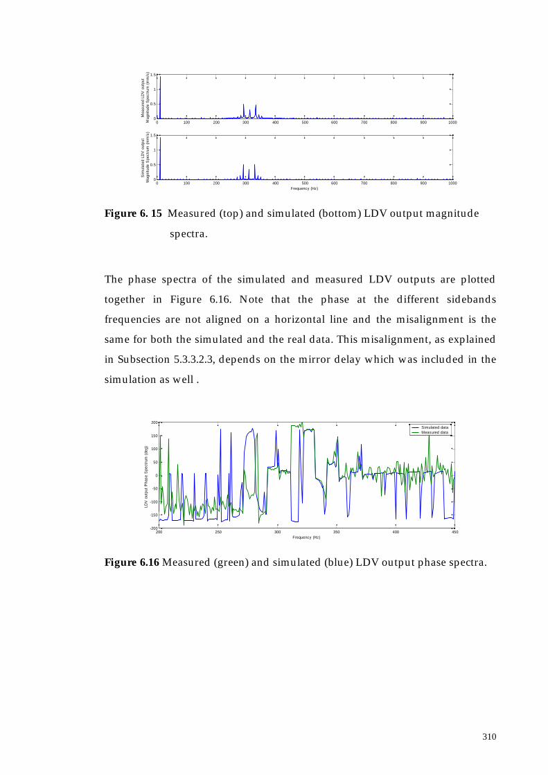
310

0 100 200 300 400 500 600 700 800 900 1000

0

0.5

1

1.5

Frequency (Hz)

Sim

ulat

ed L

DV

out

put

Mag

nitu

de S

pect

rum

(m

m/s

)

0 100 200 300 400 500 600 700 800 900 10000

0.5

1

1.5

Mea

sure

d LD

V o

utpu

t M

agni

tude

Spe

ctru

m (

mm

/s)

Figure 6. 15 Measured (top) and simulated (bottom) LDV output magnitude

spectra.

The phase spectra of the simulated and measured LDV outputs are plotted

together in Figure 6.16. Note that the phase at the different sidebands

frequencies are not aligned on a horizontal line and the misalignment is the

same for both the simulated and the real data. This misalignment, as explained

in Subsection 5.3.3.2.3, depends on the mirror delay which was included in the

simulation as well .

200 250 300 350 400 450-200

-150

-100

-50

0

50

100

150

200

Frequency (Hz)

LDV

out

put

Pha

se S

pect

rum

(de

g)

Simulated dataMeasured data

Figure 6.16 Measured (green) and simulated (blue) LDV output phase spectra.

311

6.6. Averaging Procedure

In the previous section it was demonstrated that the speckle noise affecting the

measurements performed by continuous scanning techniques is periodic with a

basic period at the frequency of the motion of the measuring laser beam, and,

specifically, although the amplitude of the noise is random, its effect occurs

located at the same phase datum. It was then thought that the easiest solution of

the problem would be to average the time histories acquired each time within

one complete scan (say backwards and forwards if it was considered a line

scan) taking care to start the acquisitions always at the same position over the

line (this is made possible by triggering the acquisition with the mirror driver

signal). Another solution has been found in the use of velocity data acquired

over several cycles of the laser scan. The signal could, then, be cut into a

number of sub-signals, each of them corresponding to an unique complete cycle

of scanning of the laser along the line traveled. Therefore, all these pieces could

be averaged in order to remove the periodic noise and reassembled together

again to give a new “filtered” time history free from the speckle noise.

As an example, where it was decided to show the feasibility of the idea of

averaging, the time histories measured, when performing a straight-line scan at

10 Hz on the beam shown in Figure 5.1, were considered. The same

experimental data used for the validation of the analysis of the line scan

technique described in Subsection 5.3.3.3 were employed here, specifically the

averaging procedure was applied to the time signal acquired when the beam

was excited at the third and fifth natural frequencies (311 and 766 Hz).

Figure 6.17 illustrates the time history and the spectral content in magnitude of

the LDV output when the beam was excited at 311 Hz.

From both plots, in the time and the frequency domains the important presence

of the 10 Hz component is clear and from the zoomed FFT plotted in Figure 6.18

all the harmonics of 10 Hz are visible.

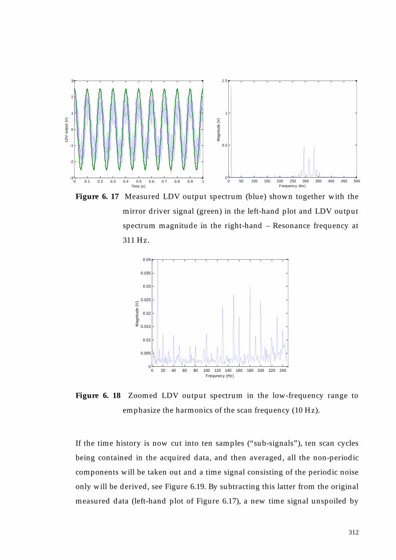
312

Figure 6. 17 Measured LDV output spectrum (blue) shown together with the

mirror driver signal (green) in the left-hand plot and LDV output

spectrum magnitude in the right-hand – Resonance frequency at

311 Hz.

0 20 40 60 80 100 120 140 160 180 200 220 2400

0.005

0.01

0.015

0.02

0.025

0.03

0.035

0.04

Frequnecy (Hz)

Mag

nitu

de (

V)

Figure 6. 18 Zoomed LDV output spectrum in the low-frequency range to

emphasize the harmonics of the scan frequency (10 Hz).

If the time history is now cut into ten samples (“sub-signals”), ten scan cycles

being contained in the acquired data, and then averaged, all the non-periodic

components will be taken out and a time signal consisting of the periodic noise

only will be derived, see Figure 6.19. By subtracting this latter from the original

measured data (left-hand plot of Figure 6.17), a new time signal unspoiled by

0 0.1 0.2 0.3 0.4 0.5 0.6 0.7 0.8 0.9 1-3

-2

-1

0

1

2

3

TIme (s)

LDV

out

put

(V)

0 50 100 150 200 250 300 350 400 450 5000

0.5

1

1.5

Frequency (Hz)

Mag

nitu

de (

V)

313

the noise is obtained, see Figure 6.20, where the right plot is a zoom of the left

one.

0 0.1 0.2 0.3 0.4 0.5 0.6 0.7 0.8 0.9 1-3

-2

-1

0

1

2

3

Time (s)

Ave

rage

d T

ime

Sig

nal (

V)

Figure 6. 19 Averaged time signal (blue) and mirror driver signal (green).

0 0.1 0.2 0.3 0.4 0.5 0.6 0.7 0.8 0.9 1-3

-2

-1

0

1

2

3

Time (s)

Filt

ered

Tim

e H

isto

ry (

V)

Figure 6. 20 Time history deprived of the periodic noise (blue) and mirror

driver signal (green) – Resonance frequency at 311 Hz.

It is already evident by inspecting the filtered time signal that the periodic

component due to the speckle pattern motion at the same frequency of the

scanning laser beam is completely eliminated. In Figure 6.21 the effect is

emphasised: the spectral contents of the original time history and the processed

314

one are plotted together. The left-hand plot shows how the components at the

excitation frequency (311 Hz) and its sidebands are completely coincident while

the right-hand plot highlights that the filtered spectrum does not contain

anymore any components at 10 Hz and its harmonics2.

Figure 6.22 depicts the magnitude of the FFT of both the signals (original in the

left plot and filtered in the right) in order to have a quantitative description of

the floor noise reduction. In the measured signal the floor noise level was at –

30 dB (40 dB less than the vibration peak which was at 10 dB); in the filtered

signal the noise floor drop at –43 dB (53 dB less of the vibration peak which was

not changed). The noise then drops from 1% re the vibration peak to 0.2 %.

Figure 6. 21 Spectral components of the original time history (blue) and the

filtered one (green). The left plot is a zoom in the low-frequency

range – Resonance frequency at 311 Hz.

2 In this section it was stated that the averaging procedure allows eliminating the periodic component dueto the speckle pattern motion. It should be highlighted again that the periodicity of the speckle noiseconcerns only the phase while its amplitude is random. Therefore, it is possible to get rid of the specklenoise by averaging. On the other hand the vibration component of the signal is periodic in amplitude andphase; the averaging will, then, not produce any effect on it.

0 50 100 150 200 250 300 350 400 450 5000

0.5

1

1.5

Frequency (Hz)

Mag

nitu

de (

V)

0 50 100 150 200 2500

0.005

0.01

0.015

0.02

0.025

0.03

0.035

0.04

Frequency (Hz)

Mag

nitu

de (

V)

315

Figure 6. 22 Fourier spectrum amplitude in dB for the original measured signal

(left) and the filtered one (right) – Resonance frequency at 311 Hz.

The same procedure can be applied to the time history acquired when the beam

was excited at 766 Hz, see Figure 6.23 where the LDV output is shown in the

time (left) and frequency domain (right). This case is interesting since the level

of the structural vibration was higher than the previous case (third natural

frequency). Therefore, it was found to be hard to maintain the focus of the laser

spot in the structure stable. The classical frequency broadening (as described in

Section 2.5 and experimentally shown in Subsection 5.5.4.3, specifically in

Figure 5.78) was noticed, namely the group of sidebands around the excitation

frequency was repeated at the double of the excitation frequency value (1532

Hz), as it is clear in the right plot of Figure 6.23.

Since the spectral component at the double of the excitation frequency and its

sidebands are due to the speckle noise which is periodic, one would expect that

its contribution will be reduced if not completely eliminated. The right plot of

Figure 6.24, where the FFT of the signal processed in the way described in this

section is illustrated, prove this deduction since the spectral content in the

high-frequency range is remarkably decreased. Moreover, as expected, the

Fourier components at 10 Hz and its harmonics are almost absent (the spectral

magnitude at 10 Hz was 3 V in the original measured signal while it drop to 0.3

0 100 200 300 400 500 600 700-60

-50

-40

-30

-20

-10

0

10

Frequency (Hz)

Mag

nitu

de (

dB)

0 d

B =

1 V

0 100 200 300 400 500 600 700-60

-50

-40

-30

-20

-10

0

10

Frequency (Hz)

Mag

nitu

de (

dB)

0 d

B =

1 V

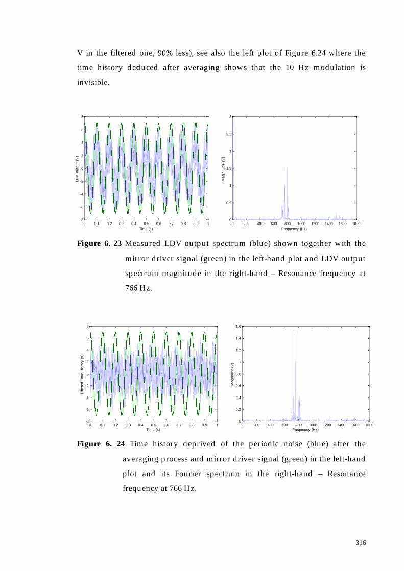
316

V in the filtered one, 90% less), see also the left plot of Figure 6.24 where the

time history deduced after averaging shows that the 10 Hz modulation is

invisible.

Figure 6. 23 Measured LDV output spectrum (blue) shown together with the

mirror driver signal (green) in the left-hand plot and LDV output

spectrum magnitude in the right-hand – Resonance frequency at

766 Hz.

Figure 6. 24 Time history deprived of the periodic noise (blue) after the

averaging process and mirror driver signal (green) in the left-hand

plot and its Fourier spectrum in the right-hand – Resonance

frequency at 766 Hz.

0 0.1 0.2 0.3 0.4 0.5 0.6 0.7 0.8 0.9 1-8

-6

-4

-2

0

2

4

6

8

Time (s)

Filt

ered

Tim

e H

isto

ry (

V)

0 200 400 600 800 1000 1200 1400 1600 18000

0.2

0.4

0.6

0.8

1

1.2

1.4

1.6

Frequency (Hz)

Mag

nitu

de (

V)

0 0.1 0.2 0.3 0.4 0.5 0.6 0.7 0.8 0.9 1-8

-6

-4

-2

0

2

4

6

8

Time (s)

LDV

out

put

(V)

0 200 400 600 800 1000 1200 1400 1600 18000

0.5

1

1.5

2

2.5

3

Frequency (Hz)

Mag

nitu

de (

V)

317

In Figure 6.25 the spectra of both the measured and the processed signal in dB

are reported to have again a quantitative representation of the noise floor

reduction: the floor noise drop from –18 dB to –25.7 dB, the maximum vibration

peak being at 3.6 dB. The noise then was reduced from 8.3% re the vibration

peak to 3.4 %.

Figure 6. 25 Fourier spectrum amplitude in dB for the original measured signal

(left) and the filtered one (right).

6.7. Conclusions

In this chapter the role of a “virtual” continuous scanning measurement has

been investigated. In order to carry out a virtual test, a simulation of a real test

has been performed by producing a mathematical model of the test which

includes the actual tested object’s structural behaviour when excited at one of

its natural frequencies, and the simulation of the noise that pollutes the LDV

output signal. This latter has been found to depend mostly on the laser-related

effect, which is the speckle noise. A detailed theoretical model of speckle has

then been developed and tested by comparing analytical results with real

experimental data.

From the study of speckle noise, which involved both a theoretical analysis and

the experimental observation of the phenomenon, an important deduction was

0 200 400 600 800 1000 1200 1400 1600 1800-50

-40

-30

-20

-10

0

10

Frequency (Hz)

Mag

nitu

de (

dB)

0

dB =

1 V

0 200 400 600 800 1000 1200 1400 1600 1800-50

-40

-30

-20

-10

0

10

Frequncy (Hz)

Mag

nitu

de (

dB)

0

dB =

1 V

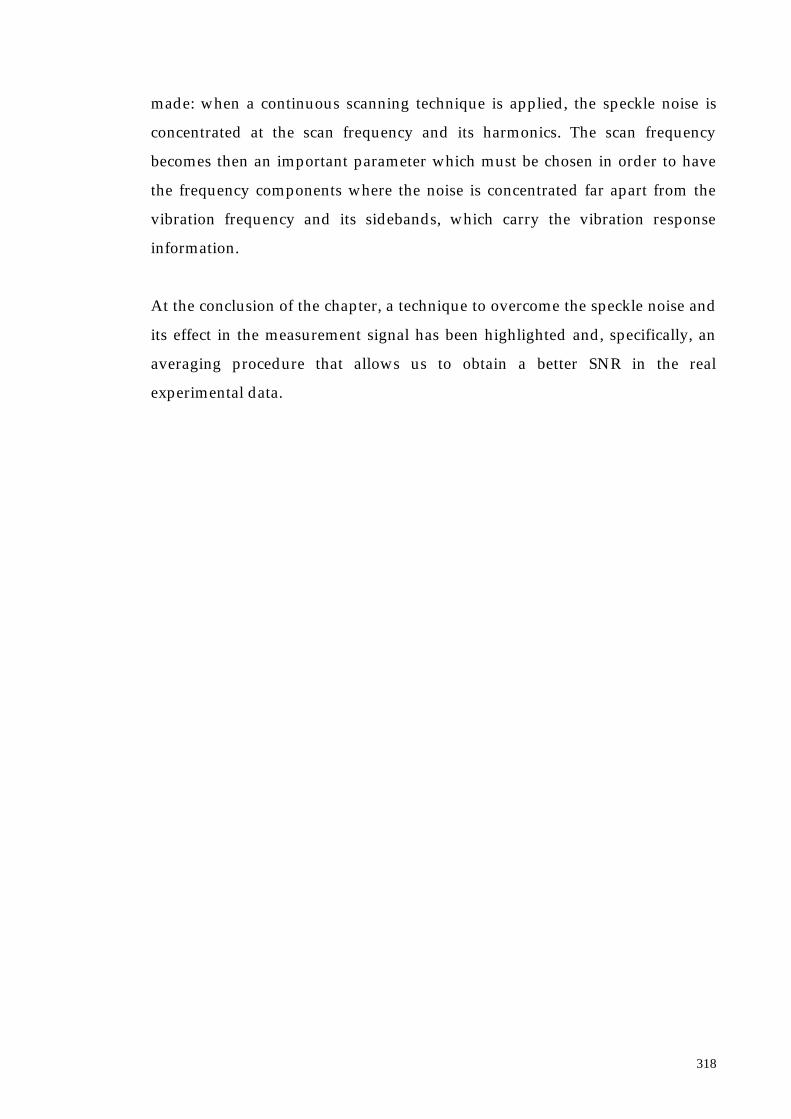
318

made: when a continuous scanning technique is applied, the speckle noise is

concentrated at the scan frequency and its harmonics. The scan frequency

becomes then an important parameter which must be chosen in order to have

the frequency components where the noise is concentrated far apart from the

vibration frequency and its sidebands, which carry the vibration response

information.

At the conclusion of the chapter, a technique to overcome the speckle noise and

its effect in the measurement signal has been highlighted and, specifically, an

averaging procedure that allows us to obtain a better SNR in the real

experimental data.

Chapter 7 Application of the ContinuousScanning Technique on IndustrialCases

7.1. Introduction

In this chapter a collection of measurements obtained with the continuous-

scanning measurement techniques described in Chapters 4 and 5 are illustrated.

Different practical applications were investigated: some case studies were taken

from structures under analysis within BRITE/EURAM projects running at

Imperial College such as QUATTRO, [47], and VALSE, [13]. A number of

different techniques were employed on these practical structures:

(i) short-line scan for 2-DOF recovery;

(ii) small-circular scan for 3-DOF determination;

(iii) long-line scan at uniform rate for direct ODS establishment, via

demodulation;

(iv) sinusoidal long-line scan for the calculation of the ODS as a polynomial;

(v) parallel sinusoidal long-line (raster) scans over an area to derive 2D ODSs;

(vi) two-dimensional long-scan at uniform rate to recover the 2D ODS via

demodulation;

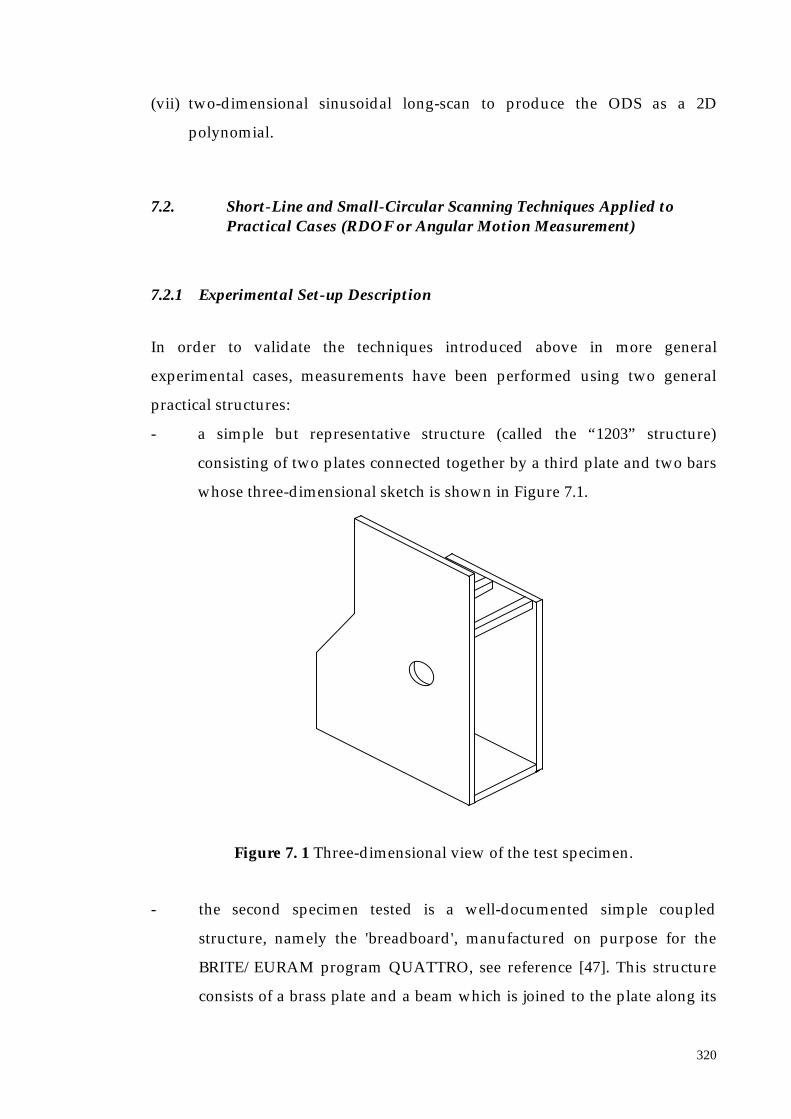
320

(vii) two-dimensional sinusoidal long-scan to produce the ODS as a 2D

polynomial.

7.2. Short-Line and Small-Circular Scanning Techniques Applied toPractical Cases (RDOF or Angular Motion Measurement)

7.2.1 Experimental Set-up Description

In order to validate the techniques introduced above in more general

experimental cases, measurements have been performed using two general

practical structures:

- a simple but representative structure (called the “1203” structure)

consisting of two plates connected together by a third plate and two bars

whose three-dimensional sketch is shown in Figure 7.1.

Figure 7. 1 Three-dimensional view of the test specimen.

- the second specimen tested is a well-documented simple coupled

structure, namely the 'breadboard', manufactured on purpose for the

BRITE/EURAM program QUATTRO, see reference [47]. This structure

consists of a brass plate and a beam which is joined to the plate along its

321

diagonal via two bolts, whose positions are shown in Figure 7.4. Figures

7.2 and 7.3 show the dimensions of plate and beam respectively.

Figure 7. 2 The brass plate.

The thickness of the plate is 3 mm. Seven holes with diameter 5 mm are drilled

in the plate. Four small holes with 2 mm diameter are also made at the plate

corners primarily for hanging the structure.

Figure 7. 3 The brass beam.

322

Figure 7. 4 Assembled structure seen from the laser head position.

A system has been developed for measuring MDOF vibration of a point,

exploiting the techniques described in the previous sections. A standard Polytec

scanning vibrometer (laser head OFV-055 and controller OFV-3001-S) is used as

the velocity transducer. The measurement process can be divided in two

separate stages: (i) the scanning control and data acquisition, where the

vibration signal from the CSLDV is stored as a time-history and (ii) the data

post-processing, in which the derivation of the required DOF responses is

made. The control and data-acquisition system has been designed using

National Instrument boards controlled by a PC platform and the management

software has been developed in LabVIEW. The control system generates the

arbitrary waveforms that must be sent to the mirrors in order to perform the

continuous scan by means of an NI two-output channels 12-bit resolution card

driven by the LabVIEW routines. In this case, since linear or circular scans are

employed, the routine is used to produce respectively one or two sinewaves of

identical amplitude and frequency and a 90° phase shift (see Appendix A.1.5 for

the control panel of the LabVIEW program driving the mirrors). The same PC

controls, via a GPIB, an HP 33120A 15MHz Function/Arbitrary Waveform

Generator which produces the excitation transmitted to the structure through a

bolts position

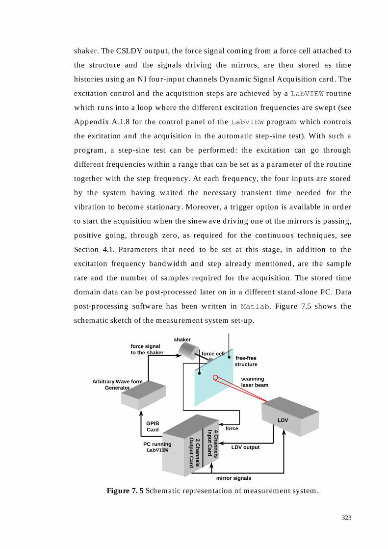
323

shaker. The CSLDV output, the force signal coming from a force cell attached to

the structure and the signals driving the mirrors, are then stored as time

histories using an NI four-input channels Dynamic Signal Acquisition card. The

excitation control and the acquisition steps are achieved by a LabVIEW routine

which runs into a loop where the different excitation frequencies are swept (see

Appendix A.1.8 for the control panel of the LabVIEW program which controls

the excitation and the acquisition in the automatic step-sine test). With such a

program, a step-sine test can be performed: the excitation can go through

different frequencies within a range that can be set as a parameter of the routine

together with the step frequency. At each frequency, the four inputs are stored

by the system having waited the necessary transient time needed for the

vibration to become stationary. Moreover, a trigger option is available in order

to start the acquisition when the sinewave driving one of the mirrors is passing,

positive going, through zero, as required for the continuous techniques, see

Section 4.1. Parameters that need to be set at this stage, in addition to the

excitation frequency bandwidth and step already mentioned, are the sample

rate and the number of samples required for the acquisition. The stored time

domain data can be post-processed later on in a different stand-alone PC. Data

post-processing software has been written in Matlab. Figure 7.5 shows the

schematic sketch of the measurement system set-up.

Figure 7. 5 Schematic representation of measurement system.

mirror signals

LDV output

forceGPIBCard

force signalto the shaker

Arbitrary Wave formGenerator

scanninglaser beam

free-freestructure

shaker

force cell

LDV

PC runningLabVIEW

4 Ch

ann

elsIn

pu

t Card

2 Ch

ann

elsO

utp

ut C

ard

324

7.2.2 Test of the “1203” Structure

The first case study consisted of the structure depicted in Figure 7.1, that was

used at the Imperial College laboratories for many comparative studies. A small

circular scan was arranged around a position on the top plate where it was

expected there would be a significant angular motion. In fact, via a previous

analysis made with the two-dimensional uniform scanning technique, see

subsection 5.5.2, a bending mode was found at 242 Hz, as shown in Figure 7.6.

The measurement set-up employed was the one shown in Figure 7.5: sinusoidal

vibration was produced in the structure by driving the shaker, whose position

is shown in Figure 7.6, in the frequency range of 200-300 Hz with an increment

of 0.5 Hz, so that the bending mode at 242 Hz would be excited. Using the

LabVIEW routines written for the purpose, the scanning mirrors were first

made to scan continuously in a circle of 11 mm radius centered at the nominal

measurement point and at a speed of 10 Hz. Then, the step-sine test was started

and, at each step, the time history coming from the LDV, triggered with the

mirror driving signal, and the output of a force cell interposed between the

shaker and the structure, were acquired and stored.

Figure 7. 6 Plate bending mode and circular scan location.

HOLEHOLE

TOP PLATE

CIRCULARSCANNINGLASER BEAM

SHAKER

xy

325

Time-domain data were then post-processed by Matlab routines written for

the purpose. The process consisted of a curve-fit of each LDV time signal at the

corresponding excitation frequency, which varied from 200 Hz to 300 Hz with a

step of 0.5 Hz, and at the sideband frequencies that were derived from the

excitation one by subtracting and adding the scan frequency (10 Hz). Thus, the

first time signal was multiplied by sine and cosine of 190, 200 and 210 Hz, and

so on for the further data. As a result, real and imaginary components of the

LDV output Fourier spectrum at each frequency step were derived: Rω, Iω, Rω−Ω,

Iω−Ω, Rω+Ω, Iω+Ω, where, ω, was the actual excitation frequency and Ω the scan

speed. These Fourier components were then scaled with the spectrum

component derived from a curve fit of the force driving signal at the relevant

excitation frequency in order to produce transfer functions - mobilities, in this

case. By applying Equation 4.15, real and imaginary components of the

translation and rotation (about both x- and y-directions) mobilities were

obtained (their magnitude plots are shown in Figures 7.7 and 7.8). RDOF

mobilities are plotted together and are multiplied by the scan radius (0.011 m)

in order to appear in the same units as the translation properties.

Figure 7. 7 Translation mobility amplitude.

200 220 240 260 280 3000

0.05

0.1

0.15

0.2

0.25

0.3

0.35

0.4

0.45

0.5

Hz

mm

/s

Tra

nsla

tion

Mob

ilty

-M

agni

tude

(m

m/s

)

Frequency (Hz)

326

Figure 7. 8 Angular mobilities amplitude.

As was expected from the previous analysis, which recovered a bending mode

at the excitation frequency of 242 Hz (see Figure 7.6) and, moreover, since the

bending was about the x-direction, the results from the small circular scan

appeared reliable. Indeed, Figure 7.8 shows a clear predominance of the x-

angular vibration.

Mobility data are visibly spoiled by noise but in order to have more accurate

measurement it is necessary to increase the resolution of the step sine test (0.5

Hz is too high), implying a more time-consuming process.

7.2.3 Test of the “breadboard” Structure

The second case study was of the so-called “breadboard” structure on which

extensive measurement of rotational degrees of freedom (RDOFs) has been

accomplished as part of the research about advanced techniques undertaken

within the BRITE/EURAM project-QUATTRO, see references [47] and [48]. The

goal of the experimental work reported here was to validate the continuous

scan technique – specifically, the linear and circular scans - for RDOFs

200 220 240 260 280 3000

0.1

0.2

0.3

0.4

0.5

0.6

0.7

0.8

0.9

Hz

mm

/s

x-rotationy-rotation

RD

OF

Mob

iltie

s -

Mag

nitu

de (

mm

/s)

Frequency (Hz)

327

recovered at a point in the structure. As a comparison technique, used to prove

the reliability of the continuos scans, a discrete point measurement was

employed with the single tested points located around the point where the

angular velocity was deduced.

The “breadboard” structure was excited in the frequency range of 300-400 Hz

with a resolution of 0.1 Hz via a shaker attached at point 37, as Figure 7.9

indicates. Then, translation and rotation degrees of freedom were derived at the

same position, using the measurement set-up shown in Figure 7.5.

Figure 7. 9 Point measurement on the “breadboard” structure.

Discrete point measurements were carried out in z-direction (perpendicular to

the structure surface) around point 37, specifically at four points slightly apart

from point 37 by a gap of 11 mm. Their positions are shown in Figure 7.10.

Figure 7. 10 Point measurement position.

The z-direction translation mobility was directly measured by pointing the

steady laser beam at point 37 (see Figure 7.11), while angular mobilities ( x

⋅θ and

point 37

laser beamlinear andcircular scans

y

x

11 mm

P1Point 37P2

P4

P3

11 mm

328

y

⋅θ ) were derived from point measurements at P1, P2, P3, and P4, using the

formulae reported in Section 4.2 (Equation 4.7):

d

frfzfrfz

y

frfzx

2

)(_)(__ 21 PP −≈

∂∂=

⋅θ (4. 1)

d

frfzfrfz

x

frfzy

2

)(_)(__ 43 PP −≈

∂∂=

⋅θ (4. 2)

d being 11 mm. Rotational mobilities about the x- and y-directions are both


Figure 7. 11 Translation mobility 37z37z – amplitude (top) and phase (bottom).

300 320 340 360 380 400-80

-60

-40

-20

0

dB re

5 m

m/s

/N

300 320 340 360 380 400-150

-100

-50

0

50

100

Hz

deg

Frequency (Hz)

329

Figure 7. 12 RDOF mobilities about x- and y-direction calculated from

translational measurements around point 37 – amplitude (top) and

phase (bottom).

Continuous linear and circular scans were directed around point 37 (see Figure

7.9) and translation and rotation degrees of freedom extracted from time-

domain signals using the Matlab routines written for this purpose.

First, linear scanning was carried out in the vertical (y) direction along a line

of 11 mm half-length and the out-of-plane translation and one rotational

mobility (z and x

⋅θ ) were derived by applying Equation 4.6; these have been

plotted together with the corresponding DOFs measured at discrete points, for

reference, in Figures 7.13 and 7.14.

Frequency (Hz)

300 320 340 360 380 400-80

-60

-40

-20

0

20

dB re

5 m

m/s

/N

300 320 340 360 380 400-150

-100

-50

0

50

100

Hz

deg

x-rotationy-rotation

Frequency (Hz)

y

x

⋅

⋅

θ

θ

330

Figure 7. 13 Translation mobility amplitude and phase derived at point 37 by

vertical line scan.

Figure 7. 14 Rotation mobility in x-direction derived at point 37 by vertical line

scan – amplitude (top) and phase (bottom).

300 320 340 360 380 400-80

-60

-40

-20

0

dB re

5 m

m/s

/N

300 320 340 360 380 400-150

-100

-50

0

50

100

Hz

deg

y-linear scan discrete points

Frequency (Hz)

300 320 340 360 380 400-60

-40

-20

0

20

300 320 340 360 380 400-150

-100

-50

0

50

100

y-linear scan discrete points

Frequency (Hz)

dB r

e 5

mm

/s/N

deg

331

Comparing translational mobilities found by discrete point measurements and

by a linear scan, see Figure 7.15, it can be noticed that results are in good

agreement: the only difference is in the narrow range between 300 to 315 Hz

where two close modes exist. The discrete point measurements detect this

feature while the linear scan in the y-direction fails to detect it. This can be

explained by the fact that this is like a bending mode along the y-axis and

therefore its deflection in the scan direction is negligible. Actually, it can be seen

from Figures 7.15 up to 7.19 that the linear scan in the x-direction and the

circular scan are more sensitive to the double modes and they can detect two

peaks also, even if their amplitudes are rather small. Consequently, it can be

deduced that the method is more accurate around than away the resonance as

the signal is small at antiresonances and therefore the effects of noise are

predominant.

Next, the same vibration responses has been measured by using a scan in the

horizontal direction (x) with a scan frequency of 10 Hz and different half-length

lines (S ) in order to investigate the effect of parameter S on the rotational

mobility. The scan in the x-direction has been repeated for S = 8, 11 and 15 mm.

The results are depicted in Figures 7.15 and 7.16 for the different values of S.


horizontal line scan with different scan length.

300 320 340 360 380 400-80

-60

-40

-20

0

dB re

5 m

m/s

/N

300 320 340 360 380 400-150

-100

-50

0

50

100

Hz

deg

S = 8 mm S = 11 mm S = 15 mm discrete points

Frequency (Hz)

332

Figure 7. 16 Rotation mobility in y-direction derived at point 37 by horizontal

line scans – amplitude (top) and phase (bottom).

Comparing the appearance of the RDOF mobility (Figure 7.16) with the

translational one (Figure 7.15), it can be seen that the first is significantly spoiled

by the noise floor. This is due to the fact that rotational components are

recovered from the Fourier spectrum sidebands whose levels are small and

often covered by the noise floor in frequency ranges which are far from

resonances.

In addition, rotational DOFs were extracted from data measured by continuous

circular scanning techniques; in this case, rotations about both the x- and y-

directions, i.e. x

⋅θ and y

⋅θ , can be recovered using Equation 4.15. The beam was

made to scan continuously in a circle of radius, R, which assumed different

values (8, 11, 15 mm) in order to investigate the influence of this parameter into

the measured data. Figures 7.17, 7.18 and 7.19 indicate the translational, x- and

y-rotational mobilities obtained at the different scan radii. In each plot, the

corresponding DOF derived by discrete measurements is shown as reference.

300 320 340 360 380 400-80

-60

-40

-20

0

20

dB re

5 m

m/s

/N

300 320 340 360 380 400-150

-100

-50

0

50

100

Hz

deg

S = 8 mm S = 11 mm S = 15 mm discrete points

Frequency (Hz)

333


circular scan with different scan radii.

Figure 7. 18 Rotation mobility in x-direction derived at point 37 by circular

scanning – amplitude (top) and phase (bottom).

300 320 340 360 380 400-80

-60

-40

-20

0

dB re

5 m

m/s

/N

300 320 340 360 380 400-150

-100

-50

0

50

100

Hz

deg

R = 8 mm R = 11 mm R = 15 mm discrete points

Frequency (Hz)

300 320 340 360 380 400-60

-40

-20

0

20

dB re

5 m

m/s

/N

300 320 340 360 380 400-150

-100

-50

0

50

100

Hz

deg


Frequency (Hz)

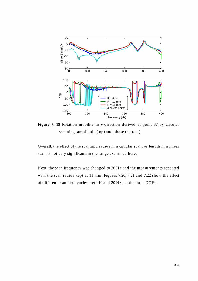
334

Figure 7. 19 Rotation mobility in y-direction derived at point 37 by circular

scanning- amplitude (top) and phase (bottom).

Overall, the effect of the scanning radius in a circular scan, or length in a linear

scan, is not very significant, in the range examined here.

Next, the scan frequency was changed to 20 Hz and the measurements repeated

with the scan radius kept at 11 mm. Figures 7.20, 7.21 and 7.22 show the effect

of different scan frequencies, here 10 and 20 Hz, on the three DOFs.

300 320 340 360 380 400-80

-60

-40

-20

0

20

dB re

5 m

m/s

/N

300 320 340 360 380 400-150

-100

-50

0

50

100

Hz

deg


Frequency (Hz)

335


circular scan with different scan speeds.

Figure 7. 21 Rotation mobility in x-direction derived at point 37 by circular

scanning- amplitude (top) and phase (bottom).

300 320 340 360 380 400-80

-60

-40

-20

0

dB re

5 m

m/s

/N

300 320 340 360 380 400-150

-100

-50

0

50

100

Hz

deg

scan speed 10 Hzscan speed 20 Hzdiscrete points

Frequency (Hz)

300 320 340 360 380 400-60

-40

-20

0

20

dB re

5 m

m/s

/N

300 320 340 360 380 400-150

-100

-50

0

50

100

Hz

deg


Frequency (Hz)

336

Figure 7. 22 Rotation mobility in y-direction derived at point 37 by circular

scanning – amplitude (top) and phase (bottom).

It was observed that by increasing the scan frequency, the resonance peaks drop

slightly, particularly for the translational DOF and rotation about the y-

direction. It is possible to explain this behaviour by referring to the speckle

noise which produces a noise floor whose level increases with the scan

frequency.

The continuous scan technique for measuring MDOF responses at a point is

convenient to use, particularly after setting up. In fact, it is less time-consuming

than a similar test done by single point measurements since with only one go,

three DOFs can be recovered simultaneously. However, in order to achieve

accurate results, the frequency step around resonances, in the step-sine

acquisition routine, often needs to be very small and this makes the

measurement time long.

300 320 340 360 380 400-80

-60

-40

-20

0

20

dB re

5 m

m/s

/N

300 320 340 360 380 400-150

-100

-50

0

50

100

Hz

deg


Frequency (Hz)

337

7.3. One-Dimensional Long - Scan Technique Application in PracticalCases

7.3.1 Experimental Set-up Description

The following experimental examples are taken from practical demonstrations

of the developed CSLDV techniques undertaken within the BRITE/EURAM

project VALSE, [13], specifically as far as regard Task 4, i.e. demonstration of

application on practical cases, see reference [23]. Measurements have been

performed (by the author) at Centro Ricerche Fiat, the VALSE partner who

leads the task related to the application to vibration transmission through

vehicles structures. Two case studies, illustrated by general views in Figure

7.23, were investigated: the rear panel of an IVECO DAILY motor lorry cab

(right) and the windscreen of a FIAT PUNTO 5door car (left). A number of

different techniques were employed, but in this section only line scans will be

considered: in particular, uniform-rate linear scans for direct ODS recovery by

LDV signal demodulation, and linear sinusoidal scans, which give ODS

polynomial coefficients.

Figure 7. 23 Vehicles used as case studies.

338

In addition, for comparison purposes, conventional point-by-point vibration

surveys were conducted using the same Polytec measurement system in its

“standard” mode and software, PSV200.

As far as concerns the truck rear panel, vibration frequency response functions

(FRFs) were measured at 375 different positions, as shown in Figure 7.24.

Figure 7. 24 Acquisition points grid –rear panel of the lory cab.

The data acquisition was performed with a sample time of 0.8 s and employing

the averaging option (specifically, five complex averages); the acquisition time

was therefore, basically (0.8 × 5 × 375) seconds., i.e. 25 mins. The actual elapsed

time for the measurement was somewhat greater than this (about 30 mins)

because of signal processing, LDV mirror reaction time, etc, see Section 3.6.

Resonant frequencies observed were: 5, 13.75, 35, 37.5, 57.5, 85, 112.5, 126.3,

137.5, 146.3, 185, 191.3, 211.3, and 230 Hz.

Similar point-by-point surveys were conducted on the FIAT Punto car front-

windscreen, to determine resonant frequencies. The screen was coated with

ADROX 9D6F spray so as to obtain a diffusing surface giving the scattered light

necessary for LDV operation. FRFs were measured on the windscreen at 382

different positions, Figure 7.25. Excitation was applied by a shaker attached on

339

the engine mounting. ODSs were measured at 25.63, 71.88, 77.5, 95, 113.1, 142.5,

185, and 240Hz, corresponding to peaks in the FRFs acquired.

Figure 7. 25 Acquisition points grid - windscreen.

For the CSLDV technique developed in this thesis the equipment used included

the same Polytec measurement head and controller employed in the SLDV

technique. In this case, however, the data acquisition, control and processing

software was completely independent from the PSV200 and it was developed in

LabVIEW. For the data post-processing Matlab routines are also available.

7.3.2 Uniform-Rate Straight-Line Scan on the IVECO DAILY Rear Panel

Continuous linear scanning measurements have been made with the LDV head

positioned about 2.5 m from the rear panel of the truck in such a way that the

laser beam at its home position (i.e. without any deflection sent to the mirrors

drivers) would be effectively perpendicular to the panel surface. The laser beam

was scanned at a uniform rate along a line A-B, shown in Figure 7.26 (i.e. the

mirror driver was fed with a triangular wave). The length of the scan was 1.406

m. The LDV output was acquired and post-processed for two different scan

speeds of the laser beam, at 0.5 Hz (1.406 m/s), and 1 Hz (2.812 m/s). The

structure was excited at one of its natural frequencies (146.3Hz) via a shaker

attached at the bottom right of the panel, as shown.

340

Figure 7. 26 Linear scan at the middle of the panel.

By running the LabVIEW acquisition program, the LDV output, triggered with

the mirror driving signal, the excitation force signal, and the triangular wave

driving the mirror were stored (using 10000 samples for each signal and a

sample rate of 1000 Hz). Data acquisition at one test frequency therefore took 10

seconds, although, strictly, only one half-scan is necessary, taking, at 0.5 Hz, just

1 sec, or 0.5 sec with at 1 Hz scan.

In order to have the same ODS information with the point-by-point technique a

set of points lying along the line A-B must be measured. In the experiment

shown in subsection 7.3.1 the line A-B contains 15 points, see Figure 7.27.

Figure 7. 27 Line scan superimposed to the grid of points used in the point-by-

point technique.

A

B

EXCITERPOSITION

A

B

341

With the point-by-point technique (where the acquisition timeat each position

of the laser beam was of 0.8 secs and 5 averages for each point were made), the

overall time needed for the acquisition of 15 points would be 4 secs. However,

as already stated (see Section 3.8), a comparison between the acquisition time

required for the continuous scanning technique and the point-by-point

technique is somewhat ambiguous. In fact, with a point-by-point technique a

broad-band excitation is applied and, consequently, in one measurement a lot

of data in the frequency domain are collected, i.e. several ODSs can be

measured in one go. With a continuous scanning technique only one ODS at the

time is measured, instead, since the excitation must be sinusoidal at the

resonance frequency. On the other hand, with a CSLDV measurement a lot of

data in the spatial domain can be collected, since the resolution of the recovered

ODS depends, in the case of uniform-rate scan, on the scan speed and the

sample rate set in the acquisition (i.e. in the actual experiment, where the scan

speed was 0.5 Hz and the sample rate 1000 Hz the ODS was measured with a

spatial resolution of 1000 points). On the contrary, with the point-by-point

technique the spatial resolution depends on the measured number of points

along the line.

Figure 7.28 shows the LDV output (black) and the mirror driver triangular

wave (in red) for two complete scans and two half-scans for the 0.5 Hz scan

(left) and the 1 Hz scan (right).

Figure 7. 28 Time histories (V) for 0.5Hz (left) and 1 Hz (right) scan speed –

LDV output (black), mirror driver signal (red).

0 0.5 1 1.5 2 2.5 3-4

-3

-2

-1

0

1

2

3

4

0 0.5 1 1.5-4

-3

-2

-1

0

1

2

3

4

Time (s) Time (s)

Tim

e si

gnal

s (V

)

Tim

e si

gnal

s (V

)

342

The post-processing of the LDV output time history consisted simply of a

demodulation at the excitation frequency together with a low-pass filtering, set

at a 50 Hz cut off frequency to reject higher components at twice the excitation

frequency. The derived ODS can easily be seen by plotting the demodulated

signal during the length of one scan (half cycle of the triangular wave); in

Figure 7.29 both the ODSs recovered for 0.5Hz scan speed and 1Hz scan speed

are shown, in their in-phase and out-of-phase components.

Figure 7. 29 ODSs in-phase and out-of-phase components (mm/s).

It may be noticed in Figure 7.29 that the 1 Hz scan speed record appears to be

less smooth than that from the 0.5 Hz scan. This is believed to be due to speckle

noise, exaggerated by the higher scan speed.

Using the PSV200 facility of selecting a profile along the ODS found by the

point-by-point scan described in subsection 7.3.1 it is possible to see the profile

of the mode along the line A-B, see Figures 7.26 and 7.27, where the line scan

was performed; Figure 7.30 shows the line where the profile was taken.

The real and imaginary components of the ODS in Figure 7.29 have been

compared with results from the pint-by-point scan measurements, Subsection

7.3.1. Data corresponding to the vertical scan line were extracted from the data

0.5 1 1.5-0.6

-0.4

-0.2

0

0.2

0.4

0.6

0.8In-Phase ODS

Scan Speed 0.5HzScan Speed 1Hz

0.5 1 1.5

-0.4

-0.2

0

0.2

0.4

0.6

0.8Out-of-Phase ODS

Scan Speed 0.5HzScan Speed 1Hz

AB BA

Dem

odul

ated

OD

S (

mm

/s)

Dem

odul

ated

OD

S (

mm

/s)

343

set derived at a frequency of 146.3 Hz using PSV200 software, and are

compared directly in Figures 7.31 and 7.32. The results clearly correspond

closely, but the coarse velocity resolution of the point-by-point survey is very

marked.

Figure 7. 30 Profile selected.

Figure 7. 31 ODS Real component (mm/s) derived by demodulation (left) and

point-by-point scan (right, the vibration response is measured at

the marked points only, where the actual measurements have

been acquired).

B

A

0.5 1 1.5-0.8

-0.6

-0.4

-0.2

0

0.2

0.4

Real Part ODS

0 0.1 0.2 0.3 0.4 0.5 0.6 0.7 0.8-0.8

-0.6

-0.4

-0.2

0

0.2

0.4

Real Part ODS

AB BA

Dem

odul

ated

OD

S (

mm

/s)

OD

S b

y pi

nt-p

oint

tech

niqu

e (m

m/s

)

344

Figure 7. 32 ODS Imaginary component (mm/s) derived by demodulation (left)

and point-by-point scan (right, the vibration response is measured

at the marked points only, where the actual measurements have

been acquired).

It should be noted that the point-by-point survey real and imaginary data were

normalised to the excitation force signal. The line scan data were adjusted

similarly for Figures 7.31 and 7.32.

Another ODS, the resonant frequency of 57.5 Hz, was investigated using the

same demodulation technique. The laser beam was scanned along a somewhat

shorter line than before, avoiding the lorry window (Figure 7.33), at a uniform

rate of 1 Hz.

Figure 7. 33 Line Scan on the panel.

0.5 1 1.5-0.3

-0.2

-0.1

0

0.1

0.2

0.3

0.4

0.5Imaginary Part ODS

0 0.1 0.2 0.3 0.4 0.5 0.6 0.7 0.8

-0.2

-0.1

0

0.1

0.2

0.3

0.4

0.5Immaginary Part ODS

AB BA

Dem

odul

ated

OD

S (

mm

/s)

OD

S b

y pi

nt-p

oint

tech

niqu

e (m

m/s

)

A

B

EXCITERPOSITION

345

The LDV output time signal together with the triangular wave driving the

mirror is shown in Figure 7.34.

Figure 7. 34 LDV output time history (V) at 57.5Hz resonant frequency.

The post-processing used was similar to that described above. In-phase and

out-of-phase ODS components are shown in Figure 7.35. Figures 7.36 and 7.37

illustrate the comparison between real and imaginary components of ODS

recovered via demodulation and by conventional Polytec PSV200 technique.

Figure 7. 35 ODSs in-phase and out-of-phase components (mm/s).

0 0.5 1 1.5-3

-2

-1

0

1

2

3

Time (s)

Tim

e si

gnal

s (V

)

0.3 0.4 0.5 0.6 0.7-0.1

0

0.1

0.2

0.3

0.4

0.5

0.6

0.7In-Phase ODS

0.3 0.4 0.5 0.6 0.7-0.1

0

0.1

0.2

0.3

0.4

0.5

0.6

0.7Out-of-Phase ODS

AB BA

Dem

odul

ated

OD

S (

mm

/s)

Dem

odul

ated

OD

S (

mm

/s)

346

Figure 7. 36 ODS Real component (mm/s) derived by demodulation (left) and

point-by-point scan (right, the vibration response is measured at the

marked points only, where the actual measurements have been

acquired).

Figure 7. 37 ODS Imaginary component (mm/s) derived by demodulation (left)

and point-by-point scan (right, the vibration response is measured

at the marked points only, where the actual measurements have

been acquired).

0.3 0.4 0.5 0.6 0.7

-0.2

-0.1

0

0.1

0.2

0.3

0.4

0.5

0.6

0.7Real Part ODS

0 0.1 0.2 0.3 0.4 0.5

-0.2

-0.1

0

0.1

0.2

0.3

0.4

0.5

0.6

0.7Real Part ODS

AB BA

Dem

odul

ated

OD

S (

mm

/s)

OD

S b

y pi

nt-p

oint

tech

niqu

e (m

m/s

)

0.3 0.4 0.5 0.6 0.7

-0.2

-0.1

0

0.1

0.2

0.3

0.4

0.5

0.6


0 0.1 0.2 0.3 0.4 0.5

-0.2

-0.1

0

0.1

0.2

0.3

0.4

0.5

0.6


AB BA

Dem

odul

ated

OD

S (

mm

/s)

OD

S b

y pi

nt-p

oint

tech

niqu

e (m

m/s

)

347

7.3.3 Sinusoidal Straight-Line Scan on the IVECO DAILY Rear Panel

A sinusoidal line scan technique was applied to the same structure, to recover

ODSs defined as polynomial series. Polynomial coefficients derived from

Fourier components of the LDV output spectrum at frequencies )( Ω±ω n ,

where ω is the excitation frequency, Ω the scan frequency and n takes integer

values from zero up to some limit set by the nature of the ODS. In order to

apply this process successfully, the ODS should ideally be spatially smooth.

Accordingly the rear panel of the lorry was excited at 57.5 Hz using the scan

line in Figure 7.33, to allow a comparison of results of the two techniques. The

laser beam was made to scan at a frequency of 1Hz.

The LDV output was acquired by running the LabVIEW program, written for

the purpose, using 20000 acquisition points with 2000 Hz sample rate. Data

acquisition, therefore, took 10 secs. The LDV time history, triggered with the

mirror-drive signal, was stored together with the (excitation) force signal and

the sinewave driving the mirror.

Part of the LDV output time signal is shown in Figure 7.38 where the mirror-

drive sine wave is included.

Figure 7. 38 LDV output time history (V).

0 0.5 1 1.5-4

-3

-2

-1

0

1

2

3

4

Time (s)

Tim

e si

gnal

s (V

)

348

The LDV output spectrum, Figure 7.39, shows the sideband structure (seen

more clearly in the zoomed, right-hand picture). Frequency broadening due to

the speckle noise, see Section 2.5, can be seen if the vertical scale is expanded,

Figure 7.40. As stated in Section 2.5, speckle noise introduces interference in the

harmonics of the excitation frequency, in this case the second harmonic (115 Hz)

is visible.

Figure 7. 39 CSLDV output spectrum and its zoom around the excitation

frequency 57.5 Hz.

Figure 7. 40 CSLDV output spectrum noise content.

Post-processing of the LDV output was done in LabVIEW, by setting the

number of sidebands included in relation to the LDV spectrum, Figure 7.39.

Fifteen sideband pairs can be seen, but they are of relatively small magnitudes

0 50 100 150 200 2500

0.05

0.1

0.15

0.2

0.25

0.3

Frequency (Hz)30 40 50 60 70 80

0

0.05

0.1

0.15

0.2

0.25

0.3

0.35

Frequency (Hz)

LDV

spe

ctru

m (

V)

LDV

spe

ctru

m (

V)

0 50 100 150 200 2500

0.005

0.01

0.015

0.02

0.025

Frequency (Hz)

LDV

spe

ctru

m (

V)

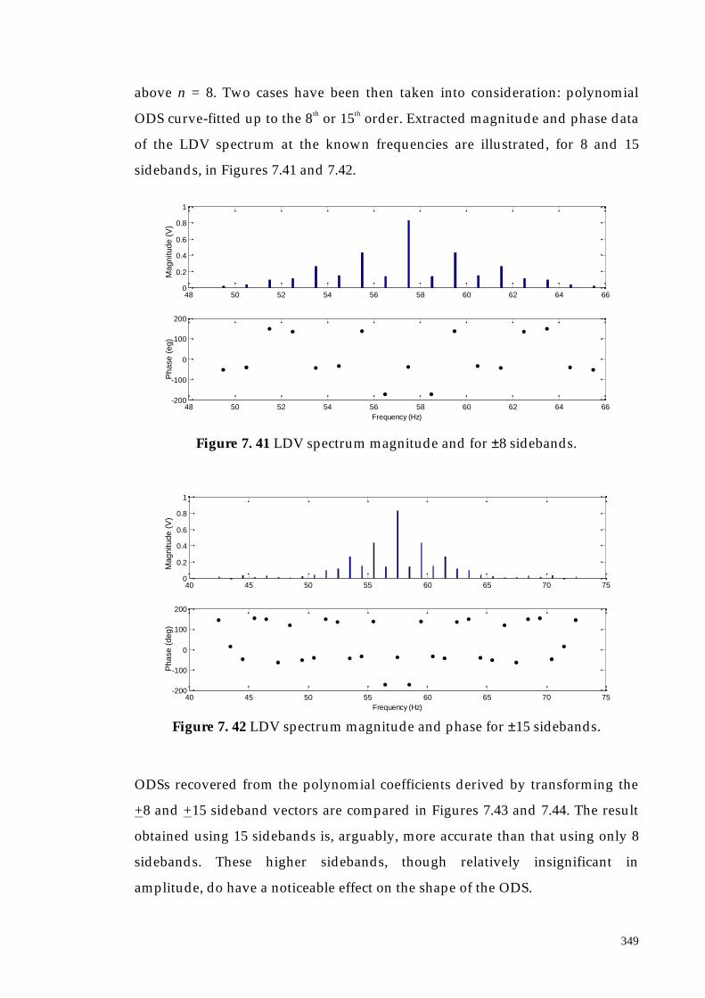
349

above n = 8. Two cases have been then taken into consideration: polynomial

ODS curve-fitted up to the 8th or 15th order. Extracted magnitude and phase data

of the LDV spectrum at the known frequencies are illustrated, for 8 and 15

sidebands, in Figures 7.41 and 7.42.

Figure 7. 41 LDV spectrum magnitude and for ±8 sidebands.

Figure 7. 42 LDV spectrum magnitude and phase for ±15 sidebands.

ODSs recovered from the polynomial coefficients derived by transforming the

+8 and +15 sideband vectors are compared in Figures 7.43 and 7.44. The result

obtained using 15 sidebands is, arguably, more accurate than that using only 8

sidebands. These higher sidebands, though relatively insignificant in

amplitude, do have a noticeable effect on the shape of the ODS.

48 50 52 54 56 58 60 62 64 660

0.2

0.4

0.6

0.8

1

48 50 52 54 56 58 60 62 64 66-200

-100

0

100

200

Frequency (Hz)

Mag

nitu

de (

V)

Pha

se (

eg)

40 45 50 55 60 65 70 750

0.2

0.4

0.6

0.8

1

40 45 50 55 60 65 70 75-200

-100

0

100

200

Frequency (Hz)

Mag

nitu

de (

V)

Pha

se (

deg)

350

Figure 7. 43 ODS real part derived by polynomial series using 8 (left) and 15

(right) sidebands.

Figure 7. 44 ODS imaginary part derived by polynomial series using 8 (left) and

15 (right) sidebands.

Finally, in Figure 7.45, the (15 sideband) sine-scan ODS is compared directly

with that obtained by demodulation, shown previously in Figure 7.35.

-1 -0.5 0 0.5 1-2

-1.5

-1

-0.5

0

0.5

1

1.5

Real Part ODS

-1 -0.5 0 0.5 1-2

-1.5

-1

-0.5

0

0.5

1

1.5

Real Part ODS

AB BA

OD

S (

V)

OD

S (

V)

± 8 sidebands ± 15 sidebands

-1 -0.5 0 0.5 1-2

-1.5

-1

-0.5

0

0.5

1

1.5

Imaginary Part ODS

-1 -0.5 0 0.5 1-2

-1.5

-1

-0.5

0

0.5

1

1.5

Imaginary Part ODS

AB BA

± 8 sidebands ± 15 sidebands

OD

S(V

)

OD

S(V

)

351

Figure 7. 45 In-Phase and Out-of-Phase ODS (V) derived by polynomial series

(± 15 sidebands) and demodulation.

7.3.4 Parallel Sinusoidal Straight-Line Scan on the FIAT PUNTO Windscreen

The technique described in subsection 7.3.3 was applied to the FIAT PUNTO

windscreen with the difference that now a series of several lines were scanned

at different positions over the surface in order to recover a raster description of

the ODS of the whole area. In practice, straight-line polynomial ODSs were

recreated from 13 sinusoidal straight-line scans, illustrated in Figure 7.46, with

excitation at 142.5 Hz and a scan speed of 1Hz. The scan lines were inclined, as

shown, to avoid areas of the curved surface where the laser beam would had a

large angle of incidence.

-1 -0.5 0 0.5 1

0

0.5

1

1.5

2

2.5

3In-Phase ODS

ODS by polynomial seriesODS by demodulation

-1 -0.5 0 0.5 1

0

0.5

1

1.5

2

2.5

3Out-of-Phase ODS

ODS by polynomial series ODS by demodulation

AB BA

352

Figure 7. 46 Windscreen sketch.

An ODS was derived for each line in the same way as described in subsection

7.3.3 for the lorry panel.

Three time histories were again acquired: specifically, the LDV output,

triggered with the sinewave driving the mirror, the force and the mirror driver

signals, using a sample rate of 1000 Hz and a number of samples of 10000

points.

Figure 7.47 shows the LDV output time signal and the mirror driver signal for

the central scan line (i.e. 7th line), and its LDV signal spectrum. This line ODS

was particularly simple in form, the spectrum has major components at only the

centre frequency and two sideband pairs. Four sidebands were included in the

signal processing in this case, to derive ODS real and imaginary components.

The sideband data extracted are shown in Figure 7.48, and the real and

imaginary ODS components in Figure 7.49.

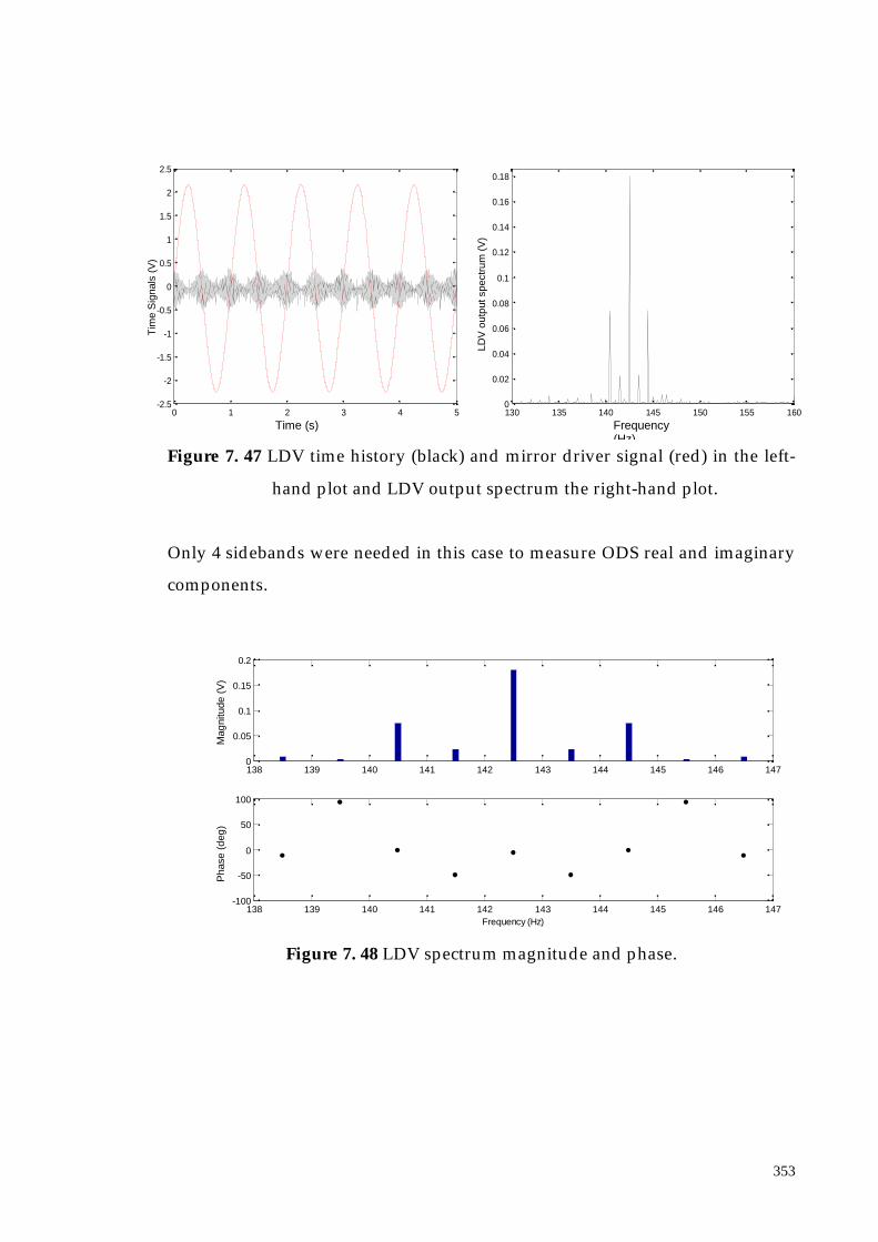
353

Figure 7. 47 LDV time history (black) and mirror driver signal (red) in the left-

hand plot and LDV output spectrum the right-hand plot.

Only 4 sidebands were needed in this case to measure ODS real and imaginary

components.

Figure 7. 48 LDV spectrum magnitude and phase.

0 1 2 3 4 5-2.5

-2

-1.5

-1

-0.5

0

0.5

1

1.5

2

2.5

130 135 140 145 150 155 1600

0.02

0.04

0.06

0.08

0.1

0.12

0.14

0.16

0.18

Time (s) Frequency(Hz)

Tim

e S

igna

ls (

V)

LDV

out

put s

pect

rum

(V

)

138 139 140 141 142 143 144 145 146 1470

0.05

0.1

0.15

0.2

138 139 140 141 142 143 144 145 146 147-100

-50

0

50

100

Frequency (Hz)

Mag

nitu

de (

V)

Pha

se (

deg)

354

Figure 7. 49 ODS Real and Imaginary components at the resonance of 142.5 Hz.

The real parts of each line-ODS are plotted together in Figure 7.50, to produce a

2-D ODS. Figure 7.51 shows the two-dimensional ODS, derived by the discrete

scan technique described in subsection 7.3.1, is illustrated.

Figure 7. 50 2-D ODS at 142.5Hz recovered by raster continuous scanningtechnique.

-2

-1

0

1

2

-3-2

-10

12

3

-0.10

0.10.2

xy

velo

city

-1 -0.5 0 0.5 1-0.4

-0.35

-0.3

-0.25

-0.2

-0.15

-0.1

-0.05

0

0.05

Real ODS

-1 -0.5 0 0.5 1-0.4

-0.35

-0.3

-0.25

-0.2

-0.15

-0.1

-0.05

0

0.05

Imaginary ODS

line start line end line start line end

OD

S (

mm

/s)

OD

S (

mm

/s)

355

Figure 7. 51 2-D ODS at 142.5Hz recovered by single point-by-point scanning

technique.

7.4. Two-Dimensional Long - Scan Technique Application to PracticalCases

7.4.1 Introduction

In order to prove the validity of the techniques described in Section 5.5 ( i.e. two

dimensional scan methods) practical case studies are addressed:

- the structure employed for MDOF continuous scanning techniques in

Section 7.2, sketched in Figure 7.1.

- the rear panel of the IVECO DAILY truck, already mentioned in Section

7.3, see Figure 7.23;

Two-dimensional area scans at uniform and sinusoidal rate were applied. In the

first case study, i.e. the irregular plate, with a cut-away section and a hole, the

demodulation technique were employed since the scanned surface and,

356

consequently, the ODS associated were not smooth. In the second example

sinusoidal area scans were achieved.

7.4.2 Two-dimensional Uniform-Rate Scan

The irregular plate was excited at one of its natural frequencies, specifically 242

Hz, and scanned by the laser beam driven by a triangular wave at 1.2 Hz in the

y-direction and at 0.02 Hz in the x-direction. In practice, the acquisition was

done in only 25 seconds, so that the x-axis was swept just once as if the x-scan

would be a linear ramp function. The data sampling rate was then 1000

Samples/s so that the scanned lines were 60 along which 25000 data points

were sampled. In order to cover the whole surface of the plate, the scan

necessarily passed over the hole and, because of its shape, outside the top left

part of the plate, see Figure 7.52.

A 100 Hz low-pass filter was used on the LDV output signal to limit speckle

noise spike amplitudes.

Figure 7. 52 Scanned area over the plate surface.

Figure 7.53 shows the complete LDV output (top plot) and the zoomed time

signal (bottom plot) depicted together with the mirrors driver signals in order

to emphasise the modulation due to the laser beam motion.

x

y

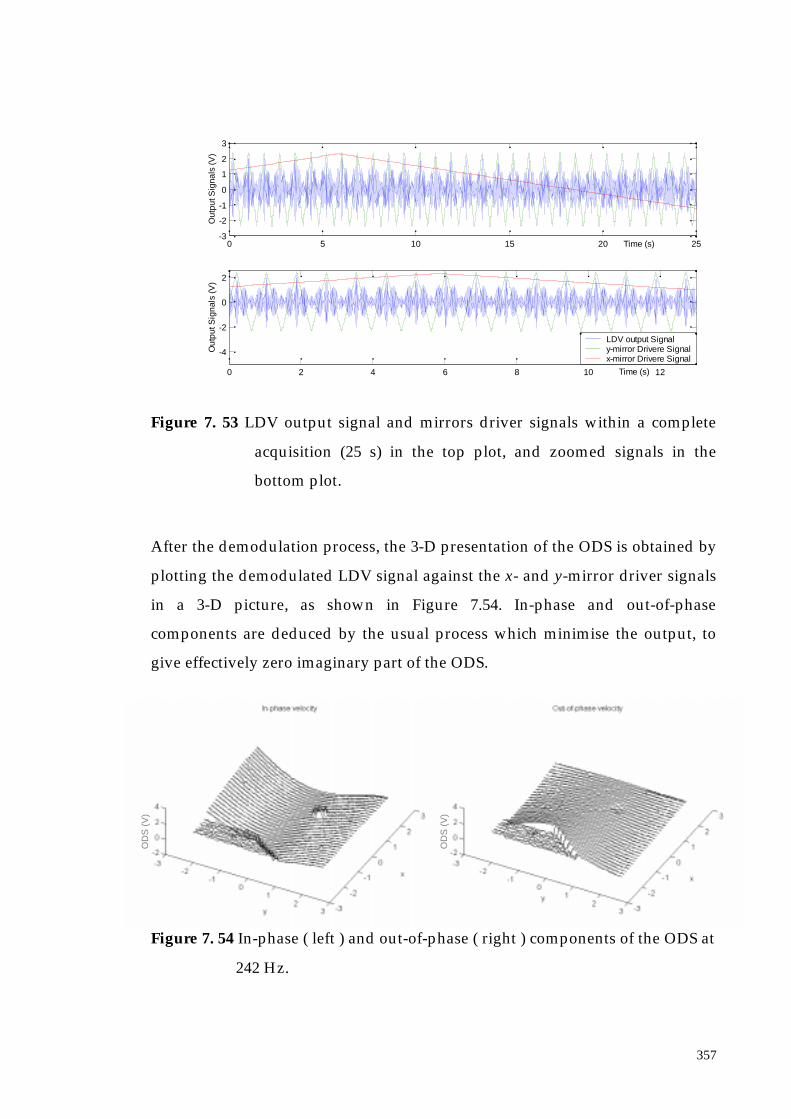
357

0 5 10 15 20 25-3

-2

-1

0

1

2

3

Time (s)

Out

put S

igna

ls (V

)

0 2 4 6 8 10 12

-4

-2

0

2

Time (s)

Out

put S

igna

ls (V

)

LDV output Signal y-mirror Drivere Signalx-mirror Drivere Signal

Figure 7. 53 LDV output signal and mirrors driver signals within a complete

acquisition (25 s) in the top plot, and zoomed signals in the

bottom plot.

After the demodulation process, the 3-D presentation of the ODS is obtained by

plotting the demodulated LDV signal against the x- and y-mirror driver signals

in a 3-D picture, as shown in Figure 7.54. In-phase and out-of-phase

components are deduced by the usual process which minimise the output, to

give effectively zero imaginary part of the ODS.

Figure 7. 54 In-phase ( left ) and out-of-phase ( right ) components of the ODS at

242 Hz.

OD

S (

V)

OD

S (

V)

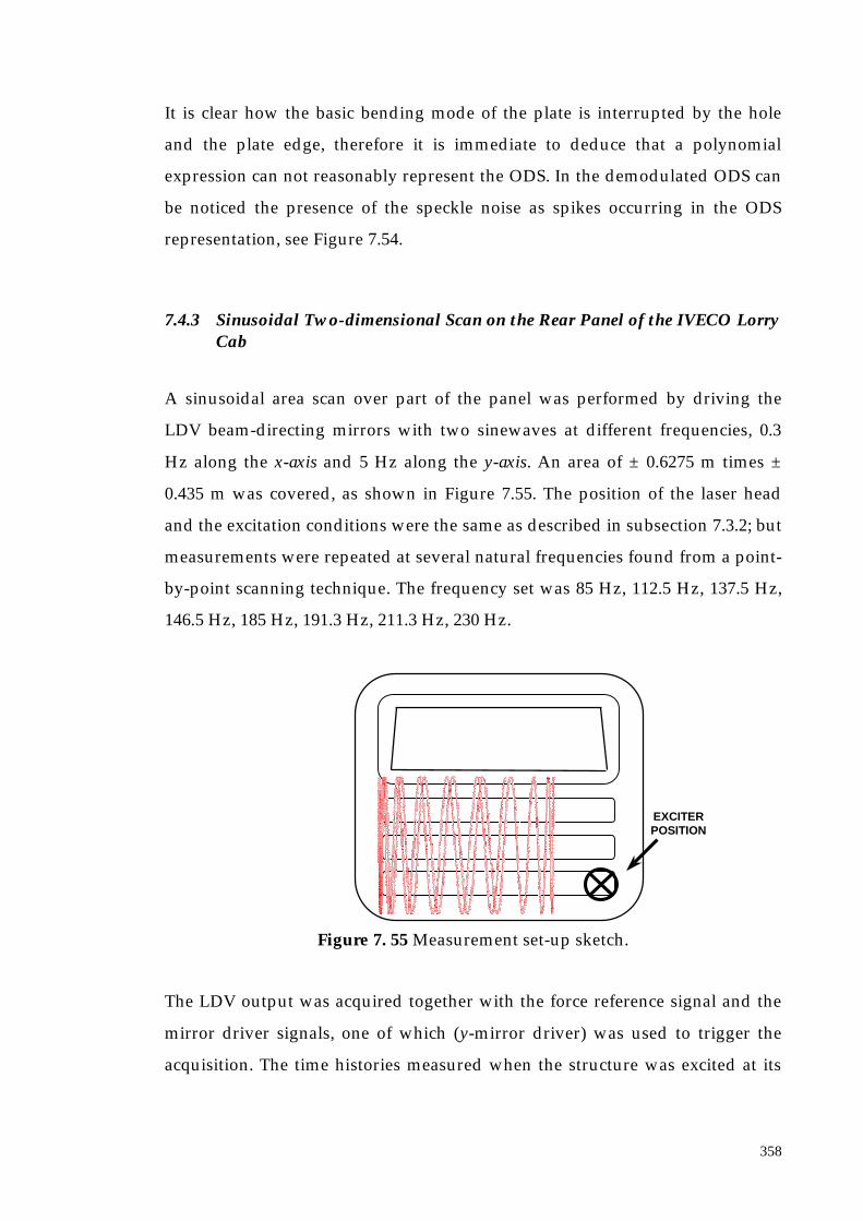
358

It is clear how the basic bending mode of the plate is interrupted by the hole

and the plate edge, therefore it is immediate to deduce that a polynomial

expression can not reasonably represent the ODS. In the demodulated ODS can

be noticed the presence of the speckle noise as spikes occurring in the ODS

representation, see Figure 7.54.

7.4.3 Sinusoidal Two-dimensional Scan on the Rear Panel of the IVECO LorryCab

A sinusoidal area scan over part of the panel was performed by driving the

LDV beam-directing mirrors with two sinewaves at different frequencies, 0.3

Hz along the x-axis and 5 Hz along the y-axis. An area of ± 0.6275 m times ±

0.435 m was covered, as shown in Figure 7.55. The position of the laser head

and the excitation conditions were the same as described in subsection 7.3.2; but

measurements were repeated at several natural frequencies found from a point-

by-point scanning technique. The frequency set was 85 Hz, 112.5 Hz, 137.5 Hz,

146.5 Hz, 185 Hz, 191.3 Hz, 211.3 Hz, 230 Hz.

Figure 7. 55 Measurement set-up sketch.

The LDV output was acquired together with the force reference signal and the

mirror driver signals, one of which (y-mirror driver) was used to trigger the

acquisition. The time histories measured when the structure was excited at its

EXCITERPOSITION

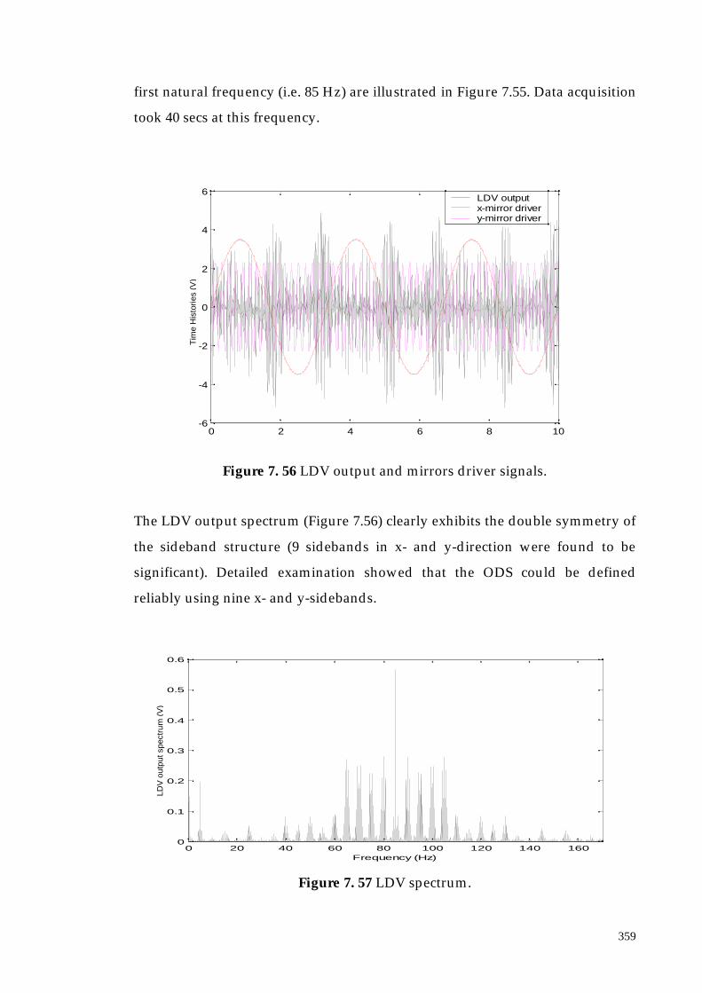
359

first natural frequency (i.e. 85 Hz) are illustrated in Figure 7.55. Data acquisition

took 40 secs at this frequency.

Figure 7. 56 LDV output and mirrors driver signals.

The LDV output spectrum (Figure 7.56) clearly exhibits the double symmetry of

the sideband structure (9 sidebands in x- and y-direction were found to be

significant). Detailed examination showed that the ODS could be defined

reliably using nine x- and y-sidebands.

Figure 7. 57 LDV spectrum.

0 2 4 6 8 10-6

-4

-2

0

2

4

6LDV output x-mirror drivery-mirror driver

Tim

e H

isto

ries

(V)

0 20 40 60 80 100 120 140 1600

0.1

0.2

0.3

0.4

0.5

0.6

Frequency (Hz)

LDV

out

put s

pect

rum

(V

)

360

Real and imaginary components of the ODS were recovered by post-processing

of the LDV output, by using LabVIEW routines developed for the purpouse. In

those programs, the mirror delay is also taken into consideration (in this case

the needed phase shift was -3.67º for the x-mirror and -5.4º for the y-mirror).

After the sideband extraction at the known frequencies (85 ± n × 5 ± m × 0.3)

Hz, assuming n and m integer values between 0 and the number of sidebands

chosen, (i.e. 9) the amplitude and phase spectrum of the LDV output appears as

the one in Figure 7.58.

Figure 7. 58 LDV spectrum amplitude (in V) and phase (in deg).

Real and imaginary ODSs recovered by transforming the sideband matrix

derived from the LDV spectrum are shown in Figure 7.59. The same ODS,

found via a discrete scan, is shown in Figure 7.60.

40 50 60 70 80 90 100 110 120 1300

0.1

0.2

0.3

0.4

0.5

0.6

Frequency (Hz)

40 50 60 70 80 90 100 110 120 130-200

-150

-100

-50

0

50

100

150

200

Frequency (Hz)

Mag

nitu

de (

V)

Pha

se (

deg)

361

Figure 7. 59 Real and Imaginary ODS at 85 Hz.

Figure 7. 60 ODS derived by discrete scan, showing the area where the

continuous scan was perormed.

ODS plots derived for each of the other natural frequencies in the set are

included as Figures 7.61 to 7.67.

OD

S (

mm

/s)

OD

S (

mm

/s)

362

Figure 7. 61 Real and Imaginary ODS at 112.5 Hz.

Figure 7. 62 Real and Imaginary ODS at 137.5Hz.


OD

S (

mm

/s)

OD

S (

mm

/s)

OD

S (

mm

/s)

OD

S (

mm

/s)

OD

S (

mm

/s)

OD

S (

mm

/s)

363




OD

S (

mm

/s)

OD

S (

mm

/s)

OD

S (

mm

/s)

OD

S (

mm

/s)

OD

S (

mm

/s)

OD

S (

mm

/s)

364


In the last two modes, the imaginary ODS component was relatively large. Its

effect was very noticeable in an ODS animation, in which travelling wave

components could be clearly seen.

7.5. Conclusions

Several continuous scan LDV techniques, developed and analysed in Chapters

4 and 5, have been applied to practical case studies in this chapter. In some

cases, together with the continuous methods, a conventional point-by-point

survey has been performed in order to have a basis of comparison for the new

techniques.

The most important advantage of the CSLDV was found to be the time-saving.

In fact a point-by-point survey took about 30 mins, compared with a 2D-area

survey in 40 secs. In reality the point-by-point technique employed a broad-

band excitation giving responses at, effectively, 1600 different frequencies,

whereas the area scan only provided data at the one test frequency. On the

other hand, having obtained broadband spectrum data, response ODSs are, in

practice, usually only required at a few natural frequencies. Moreover, the

spatial resolution of the discrete scan methods is given by the number of points

where the measurements took place (the maximum number of point is

512×512).

OD

S (

mm

/s)

OD

S (

mm

/s)

365

In contrast, on the continuous scanning technique two cases can be outlined: (i)

continuous scans at uniform rate and (ii) continuous sinusoidal scans. In the

first case the ODS spatial resolution depends on the laser scanning speed and

the sample rate employed in the acquisition process, see subsection 7.3.2, i.e. it

is limited by the acquisition system performance only. In the second case

(continuous sinusoidal scanning technique) the ODS spatial resolution is

completely arbitrarily. In fact, the ODS is derived as a polynomial whose

coefficients are derived from the measured LDV output spectrum components

at the vibration frequency and its sidebands. The resolution used for the

representation of this polynomial can then be chosen in an arbitrary way

completely independent from the acquisition parameters.

Chapter 8 Conclusions and Suggestions forFurther Work

8.1. Overall Conclusions

The primary objective of the research described in this thesis was to explore

continuous scanning laser Doppler vibrometry in all its facets by analysing the

working principles and the experimental application of each different

technique, i.e. short linear, small circular, conical and conical-scans (see Chapter

4) and long one-dimensional and two-dimensional scans (see Chapter 5). Modal

analysis applied on FRF data measured by CSLDV techniques (specifically,

sinusoidal area scans) by performing step-sine tests are addressed in Chapter 5,

see Section 5.6.

One important specific topic in this thesis is the exploration of the laser

techniques possibilities when used in the continuous scanning operation. This

implies that a detailed investigation of the laser-related phenomenon of speckle

noise (which is the main cause of pollution of measured data in LDV

technology) has been undertaken. In Chapter 2 the phenomenon is introduced

and illustrated while in Chapter 6 a model of speckle noise is outlined in order

367

to be able to include in the CSLDV test model the contribution of the noise as

well. The investigation of the speckle noise phenomenon led to the following

conclusions:

1) first, the frequency broadening of the LDV output spectrum has been

explored (Section 2.5). Because of the speckle noise, the LDV signal presents

an output spectrum with components not only at the vibration frequency

but also at its harmonics. By performing a statistical analysis of the light

intensity received by the photodetector collecting the light backscattered

from the vibrating tested surface, it was found that the most important

parameter governing the broadening of the LDV spectrum is the laser beam

width at its intersection with the object surface, i.e. the focus of the laser

spot. By carefully maintaining the laser beam focus on the vibrating object

during the measurement, the frequency broadening can be reduced to the

point where it is almost imperceptible;

2) secondly, the nature of the speckle noise when the measuring laser beam

scans continuously over the surface of a vibrating surface can be explained.

It was shown that the noise is concentrated at the scan frequency and its

harmonics. Consequently, by arranging the scan speed in relation to the

vibration frequency that needs to be measured, the frequency range of

interest in the post-processing for the vibration response recovery (i.e. the

vibration frequency and its sidebands) can be made to lie far apart from the

scan frequency harmonics. The spectral components at the resonance

frequency and its sidebands can then be almost free from speckle noise.

8.2. Summary of the Major Conclusions

8.2.1 Development of the CLSDV Techniques for MDOF Vibration Response

and ODS Measurements

The first objective of the work described in this thesis was to develop

continuous scanning methods by analysing their working principles. For

368

detailed discussion and remarks concerning the specific results obtained, the

conclusions section of each chapter (Sections 2.11, 3.8, 4.7, 5.7, 6.7 and 7.5) can

be consulted.

However, in summary, the following observations may be made in the analysis

of the CSLDV technology applied to vibration measurement:

1) CSLDV technology has been shown to be reliable when applied to

MDOF vibration response measurements. As demonstrated in Chapter 4,

where experiments in a simple cube specimen were undertaken, and in

Chapter 7 (Section 7.2), where practical structures were tested, the

technique resulted to be a reliable new method for rotational degrees of

freedom measurement.

2) As far as CSLDV application to ODS measurements is concerned, it is

concluded that the main advantage is the high spatial resolution with

which the ODS can be represented. In fact, with the ODS being expressed

as a polynomial series derived from the spectral components of the LDV

output at the vibration frequency and its sidebands, the resolution used

for its representation is completely arbitrary. This is different to the

results when a traditional point-by-point scanning technique is used, see

Chapters 3, 5 and 7. It should be pointed out as a concluding remark on

the CSLDV technology application that this method also provides a

major reduction of the quantity of data to be stored (since only the

polynomial coefficients or the spectral components of the LDV signal at

the resonance frequency and its sidebands are required for the post-

process) and a time saving on the actual test (since the time needed for

the laser beam to scan the whole surface is only a few seconds).

However, a direct comparison with the point-by-point (“standard”)

technique is difficult to make, since the experimental conditions are

different. The standard technique requires a long acquisition time but it

measures over a large frequency range while the CSLDV technique can

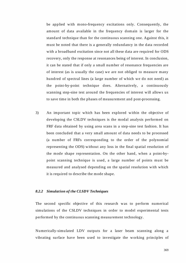
369

be applied with mono-frequency excitations only. Consequently, the

amount of data available in the frequency domain is larger for the

standard technique than for the continuous scanning one. Against this, it

must be noted that there is a generally redundancy in the data recorded

with a broadband excitation since not all these data are required for ODS

recovery, only the response at resonances being of interest. In conclusion,

it can be stated that if only a small number of resonance frequencies are

of interest (as is usually the case) we are not obliged to measure many

hundred of spectral lines (a large number of which we do not need) as

the point-by-point technique does. Alternatively, a continuously

scanning step-sine test around the frequencies of interest will allows us

to save time in both the phases of measurement and post-processing.

3) An important topic which has been explored within the objective of

developing the CSLDV techniques is the modal analysis performed on

FRF data obtained by using area scans in a step-sine test fashion. It has

been concluded that a very small amount of data needs to be processed

(a number of FRFs corresponding to the order of the polynomial

representing the ODS) without any loss in the final spatial resolution of

the mode shape representation. On the other hand, when a point-by-

point scanning technique is used, a large number of points must be

measured and analysed depending on the spatial resolution with which

it is required to describe the mode shape.

8.2.2 Simulation of the CLSDV Techniques

The second specific objective of this research was to perform numerical

simulations of the CSLDV techniques in order to model experimental tests

performed by the continuous scanning measurement technology.

Numerically-simulated LDV outputs for a laser beam scanning along a

vibrating surface have been used to investigate the working principles of

370

CSLDV techniques when applied for ODS recovery. The simulation has been

shown to be very useful to understand the detailed working of this new

measurement method.

A numerical simulation of a complete experimental test carried out by using

continuous scanning techniques has been done by means of the new approach

known as “virtual testing”. The simulated or “virtual” test model, which

includes also the simulation of the effect of the speckle noise, has been applied

for the first time to LDV testing when the laser beam is scanned across the

vibrating target structure. The description of the model and the results obtained

from the “virtual test” performed by using the model itself were shown to work

in Chapter 6 by comparing the results achieved with an actual CSLDV

experiment.

8.2.3 Experimental Validation of the CLSDV Techniques

In order to realise the objective of experimentally validating the CLSDV

techniques, simple test pieces (such as beams, plates and solid cubes) were

used. In Chapters 4 and 5, the CSLDV techniques have been tested in all their

facets and it was shown that the experimental and simulated results agreed.

Moreover, the results obtained by applying CSLDV and point-by-point

(traditional) techniques have been compared side by side. It can be concluded

that the new short scanning technique is a reliable method for measuring

rotational degrees of freedom. Indeed, this method was shown to be very

accurate in comparison with the traditional way of deriving the rotational

response of a vibrating structure by performing two translational single point

measurements and determine their first derivative.

The accuracy of CSLDV techniques was also compared with the standard point-

by-point technique when applied to the ODS recovery of vibrating structures.

In both the cases of one and two-dimensional ODSs (i.e. linear and area scans)

371

the deflection shapes of the surface derived by the two different methods were

compared with the analytical ODSs. MAC values were calculated as well (see

Subsections 5.5.4.3.2 and 5.5.4.3.3) to validate the CSLDV technique

experimental results and it was shown that this new technique works better

than the conventional point-by-point one.

8.2.4 Application of the CLSDV Techniques to Industrial Case Studies

Applications of the CSLDV techniques were made on several practical

structures (see Chapter 7) in order to prove that the technology developed in

this research works effectively in different kinds of experimental conditions

(different test surfaces: irregular plates, vehicles body, ...).

The main conclusion that can be drawn from the experiments is that the big

advantage of using CSLDV techniques by comparison with the point-by-point

ones for ODS recovery, is the effective time saving in the acquisition phase and

in the post-processing of measured data, as the applications described in this

thesis clearly show.

Continuous short-scan methods for rotational degrees of freedom

measurements have been shown to work well also on irregular structures and

to be reliable in comparison with the translational single point measurements.

Finally, demodulation techniques have been applied on an irregular plate and it

was demonstrated that the direct demodulation of the LDV output is a fast way

of obtaining the ODS of the vibrating surface and it can be applied to many

kinds of structure (i.e. with discontinuities in the measured surface). In the case

presented in Chapter 7, the tested plate presented a hole which has been

detected by the scanning laser and thus it appeared on the ODS recovered.

372

8.3. Suggestions for Further Work

In the research work described in this thesis, CSLDV techniques have been

explored and shown to have many advantages with respect to the standard

point-by-point scanning techniques. However, in this work, the continuous

scanning technology developed in this work has been confined to cases of

mono-frequency vibration. The subsequent phase of research could, then, be

directed towards the exploration of continuous scanning methods when a

general multi-frequency excitation is applied to the measured structure.

There are further opportunities for investigation of exploitation of the CSLDV

techniques to a wider range of applications, such as in the testing of machines

running under operating conditions. The continuous scanning technique has

been applied, also by the author, under conditions of self-excited excitation (i.e.

to brake disc “squeal”, see subsection 5.4.5 and reference [18]), but this

excitation was still stable at one frequency only. Therefore, the LDV technology

performance when used in cases where the excitation would not be necessarily

mono-frequency should be studied in future projects. As already stated in

Chapter 3, Section 3.1, the most important areas to be explored might be:

• CSLDV techniques applied in impact tests,

• CSLDV techniques used in case of narrow-band excitation, and

• CSLDV techniques applied in experimental configuration in which broad-

band multi-sine excitation are applied.

In conclusion, further investigations could be performed within the topic of

CSLDV measurements of structures subjected to general excitation.

References

[1] Ewins, D. J., (2000). Modal testing. Research studies press LTD.

[2] Stanbridge, A. B., Ewins, D. J., Khan, A.Z., (1998). Fault identification in

vibrating structures using a SLDV. In Proceedings of the third International

Conference on Vibration measurement by Laser Techniques, Vol.2868, pp. 449-457,

Ancona.

[3] Stanbridge A. B., Ewins D. J., (1996).Using a continuously-scanning LDV for

modal testing. In Proceedings of IMAC XIV, Dearborn.

[4] Drain, L. E., (1980). The Laser Doppler Technique. J. Wiley & Sons.

[5] Dubbeldam, G. C., (1975). In Proceedings of LDA Symposium, pp. 588-92,

Copenaghen.

[6] Bucher, I., Schmiechen, P., Robb, D. A., Ewins, D. J., (1994). A laser-based

measurement system for measuring vibration on rotating discs. In

Proceedings of the first International Conference on Vibration Measurements by

Laser Techniques, Vol. 2358, pp. 398-408, Ancona.

[7] Stanbridge, A. B., Ewins, D. J., (1995). Modal Testing of Rotating Discs using

a Scanning LDV. In Proceedings of ASME, Boston.

374

[8] Stanbridge, A. B., Ewins D. J., (1996). Measurement of translational and

angular vibration using a scanning laser Doppler vibrometer. Shock and

Vibration, Vol. 3, No. 2, pp. 141-152.

[9] Stanbridge A. B., Ewins D. J., (1996). Measurement of total vibration at a

point using a conical-scanning LDV. In Proceedings of the second International

Conference on Vibration Measurements by Laser Techniques, Vol. 2868, pp. 126-

136, Ancona.

[10] Sriram, P., Hanagud, S., Craig, J., Komerath, N. M., (1990). Scanning laser

Doppler technique for velocity profile sensing on a moving surface. In

Applied Optics, Vol. 29, No. 16, pp. 2409-2417.

[11] Sriram, P., Craig, J., Hanagud, S., (1990). A scanning laser Doppler

vibrometer for modal testing. In International Journal of Analytical and

Experimental Modal Analysis, Vol. 5, No. 3, pp. 155-167.

[12] Sriram, P., Hanagud, S., Craig, J., (1992). Mode shape measurement using a

scanning laser Doppler vibrometer. In International Journal of Analytical and

Experimental Modal Analysis, Vol. 7, No. 3, pp. 168-178.

[13] BRITE/EURAM III project VALSE, (01/02/1998-31/05/2001). A new

technology for vibration measurement of stationary and moving structures

using scanning laser Doppler velocimetry. Project reference BRPR-CT97-0594.

[14] Stanbridge, A. B., Martarelli M., Ewins, D. J., (1999). The scanning laser

Doppler vibrometer applied to impact modal testing. In Proceedings of IMAC

XVII, Orlando.

[15] Stanbridge, A. B., Martarelli, M., Ewins, D. J., (1999). Measuring area mode

shapes with a scanning laser Doppler vibrometer. In Proceedings of IMAC

XVII, Orlando.

[16] Stanbridge, A. B., Martarelli, M., Ewins, D. J., (2000). Measuring strain

response mode shapes with a continuous-scan LDV. In Proceedings of the

fourth International Conference on Vibration Measurements by Laser Techniques,

Vol. 4072, pp. 160-168, Ancona.

[17] Stanbridge, A. B., Martarelli, M., Ewins, D. J., (2000). Measuring area

vibration mode shapes with a continuous-scan LDV. In Proceedings of the

375

fourth International Conference on Vibration Measurements by Laser Techniques,

Vol. 4072, pp. 176-183, Ancona.

[18] Stanbridge, A. B., Martarelli, M., Ewins, D. J., (2001). Rotating disc vibration

analysis with a circular-scanning LDV. In Proceedings of IMAC XIX,

Kissimmee.

[19] Stanbridge, A. B., Martarelli, M., Ewins, D. J., (2001). Analysis of close mode

shapes using a scanning LDV. In Proceedings of IMAC XIX, Kissimmee.

[20] Martarelli M., Stanbridge, A. B., (1999). Measurement of translational and

rotational vibration at a point using a scanning laser Doppler vibrometer –

A users guide. BRITE/EURAM project VALSE Technical report, V2.01.

[21] Stanbridge, A. B., Martarelli M., (1999). Measurement of vibration mode

shape using a scanning LDV – A users guide. BRITE/EURAM project

VALSE Technical report, V2.02.

[22] Martarelli M., Stanbridge, A. B., (2000). Measurement of Operating

Deflection Shapes using an LDV – A users guide. BRITE/EURAM project

VALSE Technical report, V2.05.

[23] Martarelli M., Stanbridge, A. B., (2000). Application to practical case studies

- Measurement. BRITE/EURAM project VALSE Technical report, V4.01.

[24] Dainty, J. C. (1975). Laser speckle and related phenomena. Edited by J. C.

Dainty [et al.].

[25] Jackeman, E., McWhirter, J. G., (1976). Fluctuations in radiation scattered

into the Fresnel region by a random-phase screen in uniform motion.

Journal of Physics, Vol. 9, No. 5, pp. 785-797.

[26] Asakura, T., Takai, N., (1981). Dynamic laser speckles and their application

to velocity measurements of the diffuse object. Applied Physics, Vol. 25, pp.

179-194.

[27] Churnside, J. H., (1982). Speckle from a rotating diffuse object. Journal of

Optical Society of America, Vol. 72, No. 11, pp. 1464-1469.

[28] Mencuccini, C., Silvestrini, V., (1988). Physics II. Liguori.

[29] Strean, R. F., Mitchell, L. D., Barker, A. J., (1996). Global noise

characteristics of a laser Doppler vibrometer part 1: theory. In Proceedings of

376

the second International Conference on Vibration Measurements by Laser

Techniques, Vol. 2868, pp. 2-11, Ancona.

[30] Asakura, T., Takai, N., (1978). Dynamic statistical properties of vibrating

laser speckle in the diffraction field. Applied Optics, Vol. 17, No. 23, pp. 3785-

3793.

[31] Durst, F., Melling, A., Whitelaw, J. H., (1976). Principles and practice of

laser-Doppler anemometry. Academic Press.

[32] Halliwell, N. A., (2000). Short course on laser vibrometry. Fourth

International Conference on Vibration Measurements by Laser Techniques,

Ancona.

[33] Stanbridge, A. B., Khan, A. Z., Ewins, D. J., (2000). Modal testing using

impact excitation and a scanning LDV. Shock and Vibration, Vol. 7, pp. 91-

100.

[34] Vanlanduit, S., Guillaume, P., Schoukens, J., (2001). Broadband vibration

measurements using a continuously scanning laser vibrometer. In

Proceedings of IMAC XIX, Kissimmee.

[35] Castellini, P., Cupido, E., Bendel, K., (2001). Vibration measurements on

wind-screen wipers by tracking laser Doppler vibrometer. In Proceedings of

IMAC XIX, Kissimmee.

[36] Martarelli, M., Revel, G. M., Santolini, C., (1998). Automated modal

analysis by scanning laser vibrometry: problems and uncertainties

associated with the scanning system calibration. In Proceedings of IMAC

XVI, Santa Barbara.

[37] Tomasini, E. P., Paone, N., (1998). Specifications of required SLDV

performance. BRITE/EURAM project VALSE Technical report, V1.01.

[38] Leissa, A. W., (1969). Vibration of Plates. NASA SP-160.

[39] Stanbridge A. B., Ewins D. J., (1999). Modal testing using a scanning laser

Doppler vibrometer. Mechanical System and Signal Processing, Vol. 13, No. 2,

pp. 255-270.

[40] Tomasini, E. P., Castellini, P., Paone, N., (1999). Tracking of rotational

motions. BRITE/EURAM project VALSE Technical report, V3.02.

377

[41] Stanbridge A. B., Ewins D. J., (1998). Scanning laser Doppler vibrometer

measurements for vibrating beam model updating. In Proceedings of IMAC

XVI, Santa Barbara.

[42] Stanbridge A. B., Ewins D. J., (1998). Identification of dynamic properties of

beams using a scanning LDV. In Proceedings of IMAC XVI, Santa Barbara.

[43] Timoshenko, S. P., Young, D. H., Weaver, W., jr., (1974). Vibration

problems in engineering. J. Wiley & Sons.

[44] Korn, G. A., Korn, T. M., (1968). Mathematical Handbook for scientists and

engineers. McGraw-Hill.

[45] Denman, M., Halliwell, N., Rothberg, S., (1996). Speckle noise reduction in

Laser vibrometry: experimental and numerical optimisation. In Proceedings

of the second International Conference on Vibration Measurements by Laser

Techniques, Vol. 2868, pp. 12-21, Ancona.

[46] Gasparetti, M., Revel, G. M., Tomasini, E. P., (1998). Theoretical modeling

and experimental evaluation of an in-plane laser Doppler vibrometer in

different working conditions. In Proceedings of the third International

Conference on Vibration Measurements by Laser Techniques, Vol. 3411, pp. 317-

327, Ancona.

[47] BRITE/EURAM III project QUATTRO, (01/01/1998-30/09/2000).

Quantitative treatement and testing of rotational degrees of freedom. Project

reference BRPR-CT97-0540.

[48] Ziaei-Rad, S., Martarelli, M., Ewins, D. J., (2000). Measuring RDOFs using

laser Doppler vibrometer. In Proceedings of ISMA 25, Leuven.

[49] Stanbridge, A. B. , Private Communication.

[50] Rothberg, S. J., Baker, J. R., Halliwell, N. A., (1989). Laser Vibrometry:

Pseudo-Vibrations. Journal of Sound and Vibration, Vol. 135(3) pp. 516-522.

Bibliography:

Castellini, P., Revel, G.M., (1998). Damage Detection and Characterisation by

Processing of Laser Vibrometer Measurement Results: Application on

Composite Materials. In Proceedings of the third International Conference of

Vibration Measurement by Laser Techniques, Vol.2868, pp. 458-468, Ancona.

378

Jones, R., Wykes, C., (1983). Holographic and speckle interferometry. Cambridge

university press.

Beckmann, P., Spizzichino, A., (1963). The scattering of electromagnetic waves

from rough surfaces. Pergamon press.

Yamaguchi, I. Theory and applications of speckle displacement and

decorrelation. In Speckle metrology, edited by Sirohi, S.

Berne, J. B., Pecora, R., (1976). Dynamic light scattering : with applications to

chemistry, biology and physics. J. Wiley & Sons.

Li, B., Liang, J. W., Yin, C. Y., (1995). Study on the measurement of in-plane

displacement of solid surfaces by laser Doppler velocimetry. Optics & Laser

Technology, Vol. 27, No. 2, pp. 89-93.

Strean, R. F., Mitchell, L. D., Barker, A. J., (1996). Global noise characteristics of

a laser Doppler vibrometer part 2: experiments using beam dynamics. In

Proceedings of the second International Conference on Vibration Measurements by

Laser Techniques, Vol. 2868, pp. 97-105, Ancona.

Takai, N., Iwai, T., Asakura, T., (1981). An effect of curvature of rotating diffuse

objects on the dynamics of speckles produced in the diffraction field.

Applied Physics, Vol. B 26, pp. 185-192.

Churnside, J. H., Yura, H. T., (1981). Velocity measurement using laser speckle

statistics. Applied Optics. Vol. 20, No. 20, pp.3539-3541.

Ohtsubo, J., (1980). Velocity measurement using the time-space cross-

correlation of speckle pattern. Optics Communications. Vol. 340, No. 2,

pp.147-152.

Stanbridge, A. B., Martarelli M., (1999). Measurement of rotating disc vibration

using a non-synchronous circular-scanning LDV – A users guide.

BRITE/EURAM project VALSE Technical report, V3.02.

Stanbridge, A. B., Martarelli M., (1999). Conical LDV scanning on a rotating

disc. BRITE/EURAM project VALSE Technical report, V3.05.

i

APPENDIX

A.1. LabVIEW Programs

A.1.1 Shaker Control

Figure A.1 shows the LabVIEW control panel of the sine excitation generator

controlling an HP33120A arbitrary waveform generator which drives the

shaker, as described in Subsection 5.3.2.2.

Parameter settings are:

(i) Waveform generator instrument descriptor, which is the address of the

HP33120A driven via a GPIB board set in the measurement PC.

(ii) Waveform generator frequency shape (sinewave), frequency (in Hz) and

amplitude (in Volts) as required for the vibration input. Zero offset is

usually set.

ii

Figure A. 1 Shaker control panel.

A.1.2 Mirror Driver Control – Case of Scans at Uniform Rate

Figure A.2 depicts the LabVIEW control panel of the mirror driver producing

triangular waves used to feed the scanning mirrors placed on the laser head in

order to make the laser beam to scan at uniform rate (see Subsection 5.3.2.2).


(i) Device number corresponding to the output card (in this case an I/O NI

4451 with two output channels) producing the waveforms used to feed

the mirrors.

(ii) Output channels’ number.

(iii) Buffer length and sample rate adjusted to give the required resolution for

the mirror driver signals.

(iv) X- and y-waveform amplitudes (in Volts) and frequency (in Hz).

S in e

waveform shape (s ine:1 )

GP I B ::1 0

instrument descripter (1 0 )

0 .0 0

offset (0 .0 0 V )

1 8 1 .9 0

frequency (H z )

1 .0 0

amplitude ( V pp)

WAVEFORM GENERATOR FOR SHAKER CONTROL

iii

Figure A. 2 Mirror driver control panel- case of triangular waves.

A.1.3 Acquisition Control

Figure A.3 illustrates the LabVIEW control panel for the acquisition of time

histories. It is possible to acquire up to four channels, usually the LDV output,

the two mirror drivers (if a 2-dimensional scan is performed), and the reference

force signal (see Subsections 5.3.2.2, 5.3.3.3, 5.5.4.3.1).


(i) Device number corresponding to the input card (in this case an NI 4452

with four input channels).

(ii) Input channels’ number.

(iii) Trigger channel number which, specifically, corresponds to one of the

mirror driver signals.

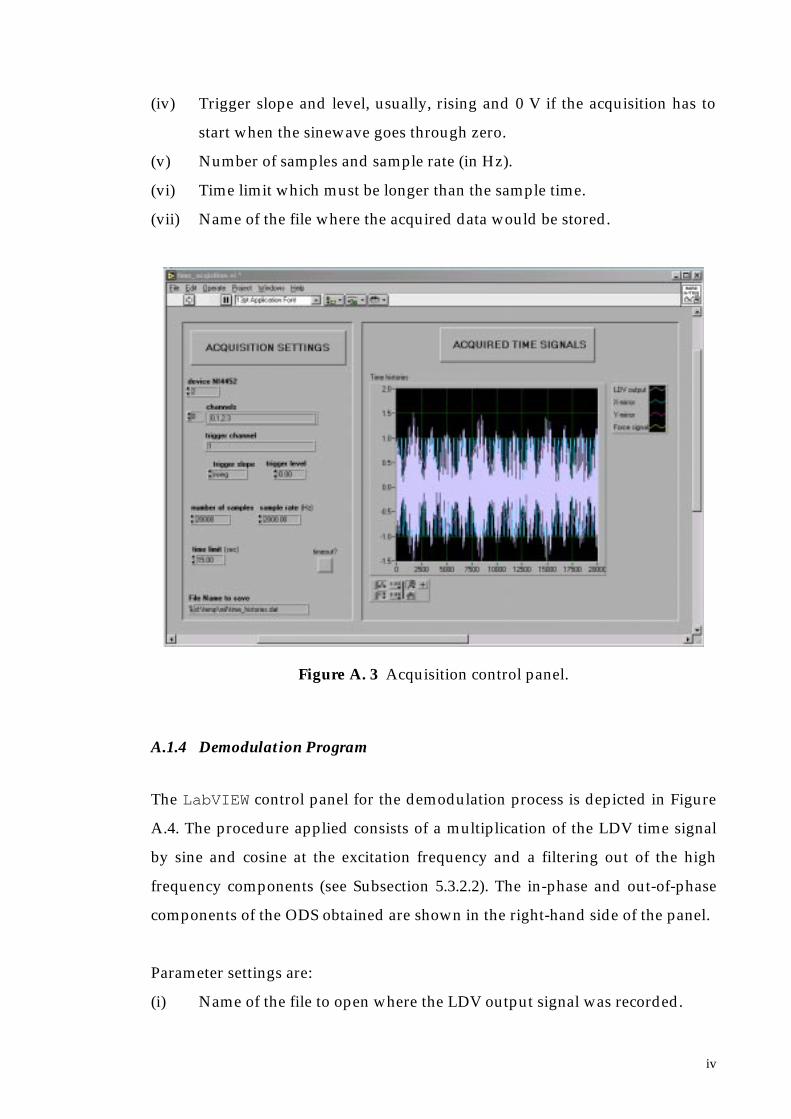
iv

(iv) Trigger slope and level, usually, rising and 0 V if the acquisition has to

start when the sinewave goes through zero.

(v) Number of samples and sample rate (in Hz).

(vi) Time limit which must be longer than the sample time.

(vii) Name of the file where the acquired data would be stored.

Figure A. 3 Acquisition control panel.

A.1.4 Demodulation Program

The LabVIEW control panel for the demodulation process is depicted in Figure

A.4. The procedure applied consists of a multiplication of the LDV time signal

by sine and cosine at the excitation frequency and a filtering out of the high

frequency components (see Subsection 5.3.2.2). The in-phase and out-of-phase

components of the ODS obtained are shown in the right-hand side of the panel.


(i) Name of the file to open where the LDV output signal was recorded.

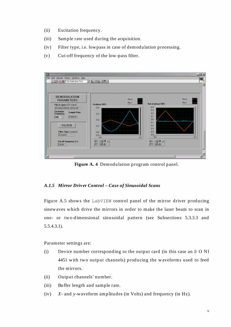
v

(ii) Excitation frequency.

(iii) Sample rate used during the acquisition.

(iv) Filter type, i.e. lowpass in case of demodulation processing.

(v) Cut-off frequency of the low-pass filter.

Figure A. 4 Demodulation program control panel.

A.1.5 Mirror Driver Control – Case of Sinusoidal Scans

Figure A.5 shows the LabVIEW control panel of the mirror driver producing

sinewaves which drive the mirrors in order to make the laser beam to scan in

one- or two-dimensional sinusoidal pattern (see Subsections 5.3.3.3 and

5.5.4.3.1).


(i) Device number corresponding to the output card (in this case an I/O NI

4451 with two output channels) producing the waveforms used to feed

the mirrors.

(ii) Output channels’ number.

(iii) Buffer length and sample rate.

(iv) X- and y-waveform amplitudes (in Volts) and frequency (in Hz).

58

vi

(v) Y-waveform phase which is usual 0° as the x-waveform phase. In the

case of circular scans, only, this value is set at 90°.

Figure A. 5 Mirror driver control panel- case of sinewaves.

A.1.6 Spectrum Analyser Program

This is a LabVIEW control program used to visualise the LDV output spectrum

(as required in Subsection 5.5.4.3.1), see Figure A.6 for the control panel.


(i) Device number corresponding to the input card (in this case an NI 4452).

(ii) Input channel’s number.

(iii) Number of samples and sample rate (in Hz).

(iv) Window to be applied to the LDV time signal.

(v) Unit of the spectral components (in Volts or dB).

(vi) Axis scale, logarithmic or linear.

vii

Figure A. 6 Spectrum analyser control panel.

A.1.7 ODS Recovery Program

This LabVIEW program performs the curve-fit of the LDV time signal and

recovers the ODS of the measured surface from the spectral components of the

LDV output at the excitation frequency and its sidebands (see Subsection

5.5.4.3.1). The control panel is split into two parts: Figure A.7 shows the part

concerning the parameter settings and the visualisation of the spectral

components of the LDV output at the frequencies of interest; Figure A.8

illustrates the final result, i.e. the real and imaginary components of the ODS.


(i) Sample rate (in Hz) used in data acquisition.

(ii) Excitation frequency (in Hz).

(iii) Number of sidebands of interest in x- and y-direction.

viii

(iv) Frequency (in Hz) of the waveforms driving the x- and y-mirror.

(v) Phase correction to be taken into account because the x- and y-mirror

delay.

(vi) Name of the file to open where the LDV output time history is stored.

Figure A. 7 ODS recovery control panel – parameter settings and spectral

components visualisation.

ix

Figure A.8 ODS recovery control panel – ODS real and imaginary components

representation.

A.1.8 Automatic Shaker Control and Acquisition Control for Step-Sine Tests

Figure A.9 shows the control panel of the LabVIEW program which controls the

excitation force applied to the shaker and the acquisition in a step-sine test

undertaken when a small circular or a short linear scan is performed on the

tested surface, see Subsection 7.2.1 for the detailed description of the procedure.

x


1) For the excitation control:

(i) Waveform generator instrument descriptor.

(ii) Waveform generator frequency shape (sinewave) and amplitude

(in Volts) .

(iii) Start excitation frequency, frequency step (in Hz) and number of

steps to be done in the step-sine test.

2) For the scanning parameters:

Scan rate (in Hz) and scan radius or scan length (in mm) if the

CSLDV technique used is a circular or a linear scan, respectively.

3) For the acquisition parameters these are the same as already described in

appendix A.1.3 for the acquisition control program.

Figure A. 9 Step-sine test control panel.

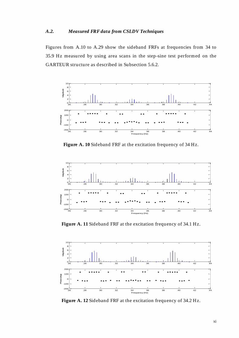
xi

A.2. Measured FRF data from CSLDV Techniques

Figures from A.10 to A.29 show the sideband FRFs at frequencies from 34 to

35.9 Hz measured by using area scans in the step-sine test performed on the

GARTEUR structure as described in Subsection 5.6.2.

26 28 30 32 34 36 38 40 42 440

2

4

6

8

10

Mag

nitu

de

26 28 30 32 34 36 38 40 42 44-200

-100

0

100

200

Frequency (Hz)

Pha

se (d

eg)

Figure A. 10 Sideband FRF at the excitation frequency of 34 Hz.

26 28 30 32 34 36 38 40 42 440

2

4

6

8

10

Mag

nitu

de

26 28 30 32 34 36 38 40 42 44-200

-100

0

100

200

Frequency (Hz)

Pha

se (d

eg)

Figure A. 11 Sideband FRF at the excitation frequency of 34.1 Hz.

26 28 30 32 34 36 38 40 42 440

2

4

6

8

10

Mag

nitu

de

26 28 30 32 34 36 38 40 42 44-200

-100

0

100

200

Frequency (Hz)

Pha

se (d

eg)


xii

26 28 30 32 34 36 38 40 42 440

2

4

6

8

10

Mag

nitu

de

26 28 30 32 34 36 38 40 42 44-200

-100

0

100

200

Frequency (Hz)

Pha

se (d

eg)


26 28 30 32 34 36 38 40 42 440

2

4

6

8

10

Mag

nitu

de

26 28 30 32 34 36 38 40 42 44-200

-100

0

100

200

Frequency (Hz)

Pha

se (d

eg)


26 28 30 32 34 36 38 40 42 440

2

4

6

8

10

Mag

nitu

de

26 28 30 32 34 36 38 40 42 44-200

-100

0

100

200

Frequency (Hz)

Pha

se (d

eg)


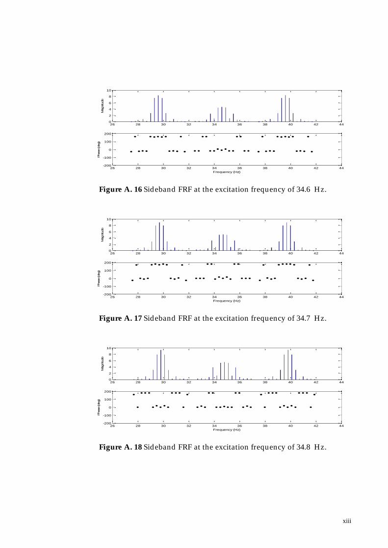
xiii

26 28 30 32 34 36 38 40 42 440

2

4

6

8

10

Mag

nitu

de

26 28 30 32 34 36 38 40 42 44-200

-100

0

100

200

Frequency (Hz)

Pha

se (d

eg)


26 28 30 32 34 36 38 40 42 440

2

4

6

8

10

Mag

nitu

de

26 28 30 32 34 36 38 40 42 44-200

-100

0

100

200

Frequency (Hz)

Pha

se (d

eg)


26 28 30 32 34 36 38 40 42 440

2

4

6

8

10

Mag

nitu

de

26 28 30 32 34 36 38 40 42 44-200

-100

0

100

200

Frequency (Hz)

Pha

se (d

eg)


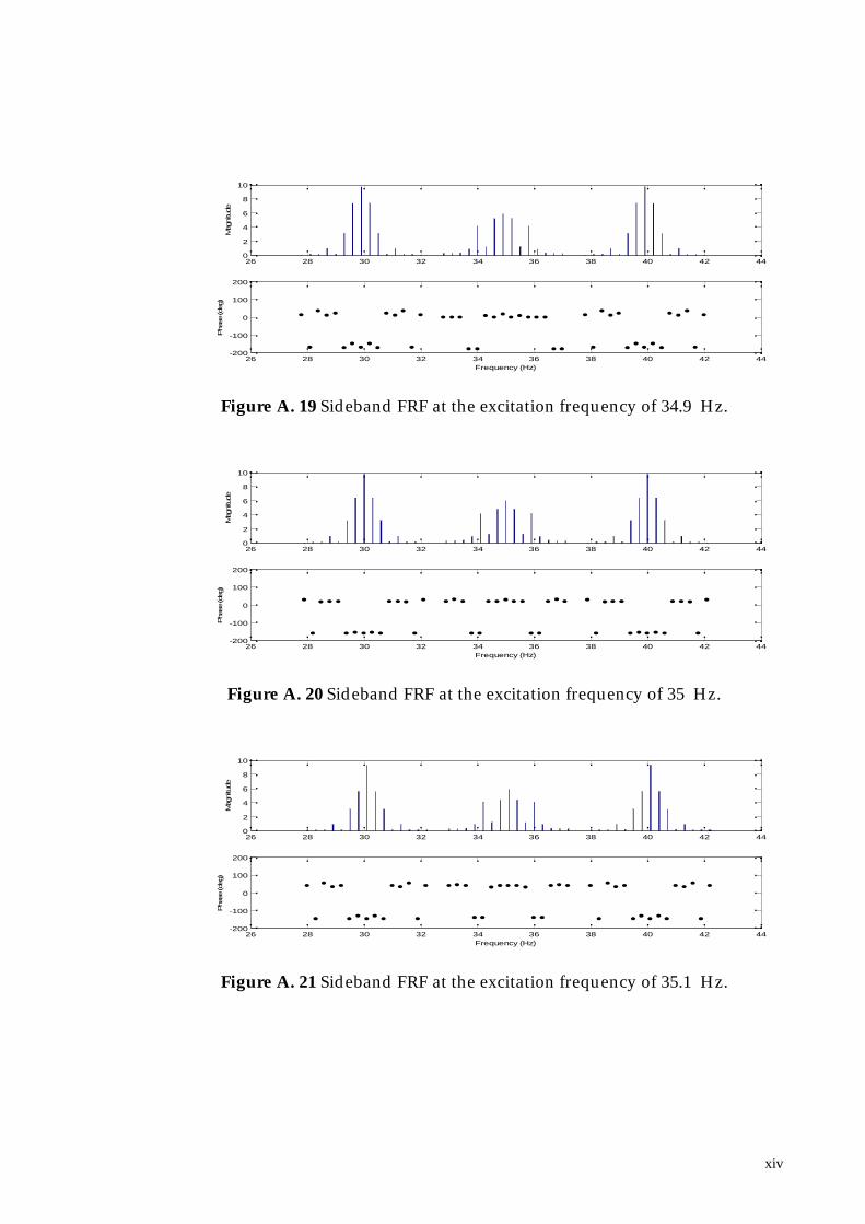
xiv

26 28 30 32 34 36 38 40 42 440

2

4

6

8

10

Mag

nitu

de

26 28 30 32 34 36 38 40 42 44-200

-100

0

100

200

Frequency (Hz)

Pha

se (d

eg)


26 28 30 32 34 36 38 40 42 440

2

4

6

8

10

Mag

nitu

de

26 28 30 32 34 36 38 40 42 44-200

-100

0

100

200

Frequency (Hz)

Pha

se (d

eg)

Figure A. 20 Sideband FRF at the excitation frequency of 35 Hz.

26 28 30 32 34 36 38 40 42 440

2

4

6

8

10

Mag

nitu

de

26 28 30 32 34 36 38 40 42 44-200

-100

0

100

200

Frequency (Hz)

Pha

se (d

eg)


xv

26 28 30 32 34 36 38 40 42 440

2

4

6

8

10

Mag

nitu

de

26 28 30 32 34 36 38 40 42 44-200

-100

0

100

200

Frequency (Hz)

Pha

se (d

eg)


26 28 30 32 34 36 38 40 42 440

2

4

6

8

10

Mag

nitu

de

26 28 30 32 34 36 38 40 42 44-200

-100

0

100

200

Frequency (Hz)

Pha

se (d

eg)


26 28 30 32 34 36 38 40 42 440

2

4

6

8

10

Mag

nitu

de

26 28 30 32 34 36 38 40 42 44-200

-100

0

100

200

Frequency (Hz)

Pha

se (d

eg)


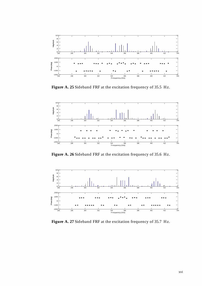
xvi

26 28 30 32 34 36 38 40 42 440

2

4

6

8

10

Mag

nitu

de

26 28 30 32 34 36 38 40 42 44-200

-100

0

100

200

Frequency (Hz)

Pha

se (d

eg)


26 28 30 32 34 36 38 40 42 440

2

4

6

8

10

Mag

nitu

de

26 28 30 32 34 36 38 40 42 44-200

-100

0

100

200

Frequency (Hz)

Pha

se (d

eg)


26 28 30 32 34 36 38 40 42 440

2

4

6

8

10

Mag

nitu

de

26 28 30 32 34 36 38 40 42 44-200

-100

0

100

200

Frequency (Hz)

Pha

se (d

eg)


xvii

26 28 30 32 34 36 38 40 42 440

2

4

6

8

10

Mag

nitu

de

26 28 30 32 34 36 38 40 42 44-200

-100

0

100

200

Frequency (Hz)

Pha

se (d

eg)


26 28 30 32 34 36 38 40 42 440

2

4

6

8

10

Mag

nitu

de

26 28 30 32 34 36 38 40 42 44-200

-100

0

100

200

Frequency (Hz)

Pha

se (d

eg)


imperial college of science, technology & medicine

Documents