implementation, analytical characterization and application of a
TRANSCRIPT

FACULTY OF SCIENCES
Department of Analytical Chemistry
X-Ray Microspectroscopy and Imaging Group (XMI)
Implementation, Analytical Characterization
and Application of a Novel Portable
XRF/XRD Instrument
Thesis submitted to obtain
the degree of Master of Science in Chemistry by
Robin DE WOLF
Academic year 2011 - 2012
Promotor: prof. dr. Laszlo VINCZE
Copromotor: dr. Bart VEKEMANS


Acknowledgments
First of all I wish to thank my promoter Prof. dr. Laszlo Vincze. Thanks to him I had the
opportunity to work with this brand new portable XRF/XRD instrument, and the chance to
visit the Deutsches Elektronen Synchrotron (DESY) facility in Hamburg which was a great and
instructive experience. I also want to thank him for the time he spend answering my questions
and the interest he showed in this master thesis topic.
Secondly, I want to thank my supervisor dr. Bart Vekemans for the help with the XRF data
processing software (AXIL and MICROXRF2) and the guidance during the measurements in
the Mayer van den Bergh museum. Thank you Bart, for the interesting conversations, for
the useful tips to perform a thorough research of the Surface Monitor, and for answering my
questions at all times.
I would like to thank dr. Ettore Di Masso and Andrea Bianco from the Assing S.p.A. company.
Thank you Andrea, for teaching me how to work with the Surface Monitor, for the nice chats
during the training, and for the repairs of the instrument.
I also want to express my gratitude to Prof. dr. Maximiliaan Martens, Prof. dr. Peter
Vandenabeele and dr. Claire Baisier (curator of the Mayer van den Bergh museum in Antwerp,
Belgium) for involving the Surface Monitor in the characterization of the “Dulle Griet” painting
and giving me the opportunity to perform measurements on this famous work of art.
Furthermore, I would like to thank the Raman Spectroscopy Research Group for providing the
painting “Colorful flowers in a vase”. This painting was used as one of the first real applications
of the Surface Monitor. Special thanks go to Prof. dr. Peter Vandenabeele, for the use of the
Olympus Innov-X DELTA handheld XRF analyzer.
I would like to thank my college master thesis student Pieter Tack for the fine moments, the
relaxing breaks and for his minimum detection limit program.
I also want to thank the members of the X-ray Microscopy and Imaging (XMI) group for their
support. Especially, Jan Garrevoet who helped me with the correction of my first thesis drafts. I
would like to express my gratitude to dr. Tom Schoonjans for his support concerning the use of
our computer infrastructure. I also want to thank Lien Van de Voorde for assisting me during
the measurements with the Olympus Innov-X DELTA handheld XRF analyzer.
iii

iv
Verder wil ik nog Jarne, Birgit, Kevin, Heleen, Bram en Jonathan bedanken, voor de gezel-
lige lunchpauzes van het voorbije jaar. Het uurtje kaarten tijdens de middag was de ideale
ontspanning tijdens dit thesisjaar.
Vervolgens zou ik ook nog graag mijn ouders willen bedanken, omdat ze mij de kans gaven deze
opleiding te volgen. Ik wil hen ook bedanken voor de ondersteuning tijdens de voorbije vijf jaar,
en omdat ze altijd klaarstonden om mij te helpen.
Tenslotte, wil ik graag mijn vriendin Stephanie bedanken, voor haar motivatie en steun gedurende
de laatste vijf jaar. Bedankt Stephanie voor de gezellige weekends, waardoor ik het thesissen
even kon vergeten.


vi

Contents
1 Objectives and Outline of the Thesis 1
2 Principles of X-Ray Fluorescence and X-Ray Diffraction 3
2.1 X-Rays: Definition and Discovery . . . . . . . . . . . . . . . . . . . . . . . . . . 3
2.2 Principles of X-Ray Fluorescence . . . . . . . . . . . . . . . . . . . . . . . . . . 4
2.2.1 Interaction of X-Rays with Matter . . . . . . . . . . . . . . . . . . . . . 4
2.3 Principles of X-Ray Diffraction . . . . . . . . . . . . . . . . . . . . . . . . . . . 8
2.3.1 Scattering of X-Rays by Electrons and Atoms . . . . . . . . . . . . . . . 9
2.3.2 Bragg’s Law . . . . . . . . . . . . . . . . . . . . . . . . . . . . . . . . . . 9
2.4 Principles of the Surface Monitor’s Components . . . . . . . . . . . . . . . . . . 10
2.4.1 X-Ray Tube Based X-Ray Production . . . . . . . . . . . . . . . . . . . 11
2.4.2 Semiconductor Based X-Ray Detection . . . . . . . . . . . . . . . . . . . 12
2.4.3 Bragg-Brentano θ : θ Set-Up . . . . . . . . . . . . . . . . . . . . . . . . 14
3 The Portable XRF/XRD Spectrometer: Assing’s Surface Monitor 15
3.1 Introduction . . . . . . . . . . . . . . . . . . . . . . . . . . . . . . . . . . . . . . 15
3.2 Description of Assing’s Surface Monitor . . . . . . . . . . . . . . . . . . . . . . 19
3.3 Methodology . . . . . . . . . . . . . . . . . . . . . . . . . . . . . . . . . . . . . 22
3.3.1 Set-Up and Positioning of the Surface Monitor . . . . . . . . . . . . . . 22
3.3.2 XRF Acquisition and Data Processing . . . . . . . . . . . . . . . . . . . 22
3.3.3 XRD Acquisition and Data Processing . . . . . . . . . . . . . . . . . . . 24
4 Results: Characterization and Applications of the Surface Monitor 29
4.1 Surface Monitor’s Performance . . . . . . . . . . . . . . . . . . . . . . . . . . . 29
4.1.1 The Laser Interferometer’s Performance . . . . . . . . . . . . . . . . . . 29
4.1.2 Optimal XRF/XRD Acquisition Distance . . . . . . . . . . . . . . . . . 32
4.1.3 Beam Size and Position of the Beam on the Sample . . . . . . . . . . . 34
4.1.4 XRF Minimum Detection Limits . . . . . . . . . . . . . . . . . . . . . . 37
4.1.5 Influence of Slits and Pinholes on XRD Spectra . . . . . . . . . . . . . . 41
4.2 Applications . . . . . . . . . . . . . . . . . . . . . . . . . . . . . . . . . . . . . . 44
4.2.1 XRF/XRD Analysis of the Painting “Colorful Flowers in a Vase” . . . . 47
4.2.2 “Dulle Griet” from Pieter Bruegel the Elder . . . . . . . . . . . . . . . . 48
vii

viii Contents
5 Summary and Conclusions 55
A Standard Reference Material 59
A.1 NIST SRM 1412 Multicomponent Glass Standard . . . . . . . . . . . . . . . . . 59
A.2 NIST SRM 660b Diffraction Standard . . . . . . . . . . . . . . . . . . . . . . . 59
B Flo2spe-Converter 63
Bibliography 67
Nederlandstalige Samenvatting 71

Chapter 1
Objectives and Outline of the Thesis
The aim of this master thesis is the establishment of the experimental methodology and the an-
alytical characterization of a novel portable X-ray fluorescence (XRF)/X-ray diffraction (XRD)
instrument called Assing’s Surface Monitor. The Surface Monitor was recently acquired from
the company Assing S.p.A. (Rome, Italy) by the Analytical Chemistry Department of Ghent
University (Belgium). This instrument is described to be used for studying art objects, e.g.
paintings and murals, by combining two powerful non-destructive analytical techniques: X-
ray fluorescence and X-ray diffraction. Before the instrument can be applied for the study
of cultural heritage objects, some questions need to be answered concerning the analytical
performance of the portable instrument. In this master thesis, the analytical figures of merit
and recommended handling of the Surface Monitor are determined. More specifically, how this
instrument must be used in order to obtain reliable and high quality XRF/XRD results.
Following the description of the objectives and outline, Chapter 2 describes the principles of X-
ray fluorescence and X-ray diffraction. Next to describing the physical properties of X-rays, also
the production of X-rays by X-ray tubes, the detection of X-rays by semiconductor detectors
and the Bragg-Brentano θ : θ set-up, used for the acquisition of XRD spectra, are discussed.
Chapter 3 gives a brief overview of already existing portable XRF/XRD instruments. Fur-
thermore, a full description of the Surface Monitor is given, including a description of the
installation/set-up procedure of the instrument and the XRF/XRD data processing.
Chapter 4 consists of two main parts. The first part describes the results of the Surface
Monitor’s characterization: characterization of the laser interferometer and the determination
of the optimal distance using this device, characterization of the beam size and its position on
the sample, calculation of minimum detection limits for XRF, and finally the influence of the
collimators on the XRD spectra. The second part of this chapter deals with two applications
of the Surface Monitor.
Finally, a summary, together with conclusions, is formulated in Chapter 5.
1

2 Objectives and Outline of the Thesis

Chapter 2
Principles of X-Ray Fluorescence
and X-Ray Diffraction
This chapter introduces the basic concepts of X-ray fluorescence (XRF) and X-ray diffraction
(XRD) that are applied when using the novel portable XRF/XRD spectrometer of the company
Assing S.p.A. [1]. Next to the physical properties of X-rays, also the production of X-rays by an
X-ray tube, the detection of X-rays by using a semiconductor detector and the Bragg-Brentano
θ : θ set-up, used for the acquisition of XRD spectra, are described in this chapter.
2.1 X-Rays: Definition and Discovery
X-rays can be classified as short wavelength electromagnetic radiation, generated in nature by
slowing electrons in the outer field of an atomic nucleus or by changing the bound states of
electrons involving transitions between the inner electronic shells of an atom. Generally the
wavelength of this type of electromagnetic radiation is lower than 10 nm (see Fig. 2.1) [2]. In
case of XRF analysis, typically radiation is used with an energy between 1 keV and 100 keV
which corresponds to a wavelength of approximately 1 nm down to 0.01 nm [3].
Figure 2.1: Spectrum of electromagnetic radiation from infrared radiation to hard X-rays (IR, infrared;
VIS, visible light; UV, ultraviolet; VUV, vacuum ultraviolet; EUV, extreme ultraviolet).
Figure adapted from Beckhoff et al. [2].
3

4 Principles of X-Ray Fluorescence and X-Ray Diffraction
Wilhelm Conrad Rontgen discovered X-rays on November 8, 1895 at the Physics Institute of
Julius-Maximilian’s University of Wurzburg, Germany. He discovered X-rays by accident while
studying cathode rays using a low pressure gas-filled discharge tube, a so called Hittorf-Crookes
tube. Near the tube he noticed a weak visible photoluminescence which was emitted by a Bar-
ium Platino-Cyanide fluorescent screen whenever the cathode-ray tube was turned on. Rontgen
recognized that this visible fluorescence was caused by “eine neue Art von Strahlen” originating
from the Hittorf-Crookes tube. Due to its unknown character, he called the radiation X-rays.
Shortly after the discovery it became clear that X-rays could be used to look into the structure
of a living human body and the interior of optically non-transparent materials [2]. In 1901
Wilhelm C. Rontgen received the first Nobel prize in physics for his work [4].
The discovery of X-rays led to some other important breakthroughs. Barkla studied the nature
of X-rays with respect to the atomic structure by observing the secondary X-rays radiated from
the target sample. During his experiments he discovered the polarization of X-rays (1906), the
gaps in atomic absorption (1909), and the distinction between continuous and characteristic
X-rays, consisting of several series of X-rays referred to as K, L, M,. . . series (1911). Building
on Barkla’s work, von Laue investigated the wave properties of X-rays. He demonstrated X-ray
diffraction from a single crystal, which was composed of a 3D-structure with a regularly repeat-
ing pattern (1912). Attracted by the experiments of von Laue, Bragg observed X-ray diffraction
patterns from single crystals of NaCl and KCl to be the regular patterns of an isometric system
showing differences in the X-ray intensity when comparing Sodium and Potassium. The ex-
periments of von Laue and Bragg formed the starting point of crystal structure analysis using
X-rays [2].
2.2 Principles of X-Ray Fluorescence
The Surface Monitor can be used to perform X-ray fluorescence (XRF) analysis. The success of
the XRF methodology is resulting from the fact that it provides a highly sensitive multi-element
compositional analysis capability, in a non-destructive manner for most elements in the periodic
system. Moreover, the interaction of X-rays with matter is essentially fully understood, giving
the researcher a powerful and practical tool to quantitavely study samples. In the following
the relevant interaction phenomena are described.
2.2.1 Interaction of X-Rays with Matter
If an X-ray beam interacts with matter, some of the incident photons are absorbed by the
sample, others are scattered away from the original direction of the incident beam and the
remaining part passes through the sample. The relation between the incoming beam intensity
(I0), passing through a sample with given thickness (x) and density (ρ), and the outgoing beam
intensity (I) is given by the law of Lambert-Beer:

Principles of X-Ray Fluorescence 5
I(x) = I0e−µρρx = I0e
−µLx (2.1)
with I0 [photons/s] the incoming X-ray beam intensity, I(x) [photons/s] the outgoing X-ray
beam intensity, x [cm] the sample thickness, ρ[g/cm3
]the sample density, µρ
[cm2/g
]the
mass attenuation coefficient and µL = µρρ[cm−1
]the linear attenuation coefficient. If the
interaction occurs in the relevant energy region of 1 − 100 keV, the mass attenuation coefficient
for a single element can be written as follows:
µρ (E,Z) = τρ (E,Z) + σρ,R (E,Z) + σρ,C (E,Z) (2.2)
with τρ (E,Z) the photoelectric cross-section, σρ,R (E,Z) the Rayleigh (elastic) scattering cross-
section and σρ,C (E,Z) the Compton (inelastic) cross-section, all function of the incident beam
energy (E) and the atomic number (Z). The relative contribution to the mass attenuation
coefficient of the three absorption effects as function of the photon energy is shown in Fig. 2.2
for three elements: Ar, Si and Ge. Eq. (2.2) is only valid if there is one element present in the
sample. For multiple elements present in the sample the mass attenuation coefficient can be
written as the sum of the weight fractions (wi) times the mass attenuation coefficient for each
element (µρ (E,Zi)) [3].
µρ (E,Z1, . . . , Zn) =
n∑
i=1
wiµρ (E,Zi) (2.3)
The three most important interactions between X-rays and atoms in the relevant region for
X-ray analysis (1 − 100 keV) are briefly discussed below. It is worthwhile to note that if higher
X-ray energies are used, pair production and photonuclear absorption will also occur. Since
these last two interaction types cannot occur at lower energies, they will not be discussed
further in this work.
Figure 2.2: Mass attenuation coefficients for the elements Argon, Silicon and Germanium. Next to the
total mass attenuation coefficient, the photoelectric, Compton and Rayleigh components
are also indicated in the graphs. Reproduced from Beckhoff et al. [2].

6 Principles of X-Ray Fluorescence and X-Ray Diffraction
Photoelectric Effect
The photoelectric effect occurs when an incident X-ray photon with energy E interacts with
a bound atomic electron, resulting in the absorption of the photon. In this case, the energy
E of the photon is completely transferred to an electron, which is ejected from the atom.
The resulting photoelectron has a kinetic energy equal to the incident photon energy (E)
minus the binding energy (E0) of the ejected electron (see Fig. 2.3). After the ejection of the
photoelectron an inner shell vacancy is created which causes an electron cascade from the outer
to the inner shells accompanied by the emission of X-ray fluorescence photons (see Fig. 2.4), or
Auger-electrons. The energies of the emitted photons are characteristic for each element and
this relationship makes X-ray fluorescence (XRF) a suitable tool for elemental composition
analysis. It was around the beginning of the twentieth century that Moseley discovered the
linear relationship between the square root of the frequency of the emitted photons and the
atomic number (see Fig. 2.5) [2].
Figure 2.3: Photoelectric effect, an X-ray photon is absorbed by an atom and a photoelectron is
ejected. Reproduced from Amptek [5].
Figure 2.4: Electron cascade from the outer to the inner shell, causing characteristic X-ray fluorescence
radiation (or the emission of Auger electrons, not shown in this figure). Reproduced from
Amptek [5].

Principles of X-Ray Fluorescence 7
Figure 2.5: The Moseley plot shows a linear relationship between the square root of the frequency of
the emitted characteristic X-ray fluorescence photons and the atomic number. Reproduced
from Vincze [3].
Scattering
Two different scattering effects occur while using X-rays: Rayleigh scattering and Compton
scattering. The difference between these two types of scattering is described in the next two
paragraphs.
During Rayleigh scattering (see Fig. 2.6) an incident photon interacts with a tightly bound
atomic electron via an elastic scattering process which implies that throughout this scattering
event the photon loses no energy. The wavelength λ1 of the incident beam is therefore the
same as the wavelength λ2 of the scattered beam.
Compton scattering is an inelastic scattering process between photons and outer shell electrons,
during which a part of the incoming photon energy is transferred to an atomic electron, the
scattered photon has a longer wavelength and lower energy than the incident photon and is
deflected by an angle θ compared to the initial direction (see Fig. 2.7). The resulting energy
of the scattered photon is given by the Compton equation:
E =E0
1 + E0mec2
(1 − cos θ)(2.4)
with E [keV] the scattered photon energy, E0 [keV] the incident photon energy, me [kg] the
electron rest mass, c [m/s] the speed of light and θ the angle between the incident photon and

8 Principles of X-Ray Fluorescence and X-Ray Diffraction
the scattered photon. The term mec2 equals 511 keV.
Figure 2.6: Rayleigh scattering (λ1, wavelength incident beam; λ2, wavelength scattered beam where
λ1 = λ2). Reproduced from Vincze [3].
Figure 2.7: Compton scattering (λ1, wavelength incident beam; λ2, wavelength scattered beam; θ,
scattering angle). Reproduced from Vincze [3].
2.3 Principles of X-Ray Diffraction
Next to X-ray fluorescence (XRF), the Surface Monitor can be used to perform X-ray diffraction
(XRD) measurements on the sample under investigation. Where XRF is capable to determine
quantitatively the elements present in the sample, XRD gives information about the arrange-
ment of the atoms in solid (crystalline) samples. It is important to mention that XRD can only
be applied on crystalline structures. Thus, a combination of these two techniques, XRF and
XRD, can provide an accurate compositional and structural characterization of the material
being studied. In a crystal, atoms are arranged in a regular pattern, which makes that a small
volume can be identified, that by repetition in three dimensions describes the whole crystal [6].
This small volume is called the unit cell and can be described by three axes: a, b and c, and
the angles between them: α, β and γ (see Fig. 2.8). A brief description is given in the next
sections.

Principles of X-Ray Diffraction 9
Figure 2.8: Unit cell parameters: α, angle between b and c; β, angle between a and c; γ, angle
between a and b. Reproduced from Jeffrey [7].
2.3.1 Scattering of X-Rays by Electrons and Atoms
From the theory of classical electromagnetism it is known that electrons, accelerated by an
alternating electric field, are oscillating with the same frequency of the field and are emitting
radiation of the same frequency of the alternating electric field (see Fig. 2.9). If atoms, from
a crystal, are exposed to an X-ray beam, all electrons around the nuclei are oscillating and
emitting radiation. Since atoms are arranged in a regular three dimensional way, constructive
interference of the scattered waves in a few directions will take place [8]. This can be described
mathematically by the von Laue equations for diffraction:
a (cos Ψa − cos Ψa,0) = hλ
b (cos Ψb − cos Ψb,0) = kλ
c (cos Ψc − cos Ψc,0) = lλ
(2.5)
where Ψx,0 is the incident X-ray beam, Ψx is the diffracted X-ray beam, a, b and c are lattice
spacings, h, k and l are natural numbers and λ is the wavelength of the incident X-ray beam
[6].
The von Laue equations (Eq. (2.5)) are very difficult to implement because in total six angles,
three lattice spacings and three natural numbers need to be defined. A mathematically more
accessible function is given by W. L. Bragg and is describe in the next section.
2.3.2 Bragg’s Law
Instead of studying the diffraction of a single electron, Bragg looked at diffraction in terms of
reflection from crystal planes (see Fig. 2.10). Two identical beams in terms of wavelength and
phase approach two layers of a crystalline solid. After interaction with two different atomic
layers, they are scattered. The beam that is scattered by the second crystal plane travels an

10 Principles of X-Ray Fluorescence and X-Ray Diffraction
Figure 2.9: Scattering by a free electron. Reproduced from Wikipedia [9].
Figure 2.10: Bragg diffraction (θ, angle between incident beam and the crystal plane; d, distance
between two crystal planes; d sin θ, path length difference between upper and lower beam).
Reproduced from Wikipedia [11].
extra length equal to 2d sin θ compared to the beam that is scattered by the upper crystal
plane. In order to obtain constructive interference this length must be equal to a positive
multiple of the wavelength of the incident radiation. This relation is mathematically described
by the famous Bragg law:
2dhkl sin θ = nλ (2.6)
where dhkl [nm] is the distance between two crystal planes, θ is the angle between the incoming
beam and the crystal plane and is also equal to the angle between the diffracted beam and the
crystal plane. λ [nm] is the wavelength of the incident beam and n is the diffraction order [10].
2.4 Principles of the Surface Monitor’s Components
The previous sections provided a general outline on the principles of XRF and XRD. In what
follows the generation and detection of X-rays as being done with the Surface Monitor is
explained. X-rays can be generated through a variety of ways by using: an X-ray tube, syn-
chrotron radiation or the radioactive decay of specific isotopes (e.g. 55Fe). Since the Surface

Principles of the Surface Monitor’s Components 11
Monitor only uses an X-ray tube the last two possibilities of generating X-rays are not dis-
cussed in this thesis. The same remark can be made for the detection of X-rays. X-rays can
be detected by using photographic plates, ionization chambers, semiconductor detectors, etc.
Since the Surface Monitor uses a semiconductor detector, only this type of detector is explained
in the following section. Next to the general working principle of the X-ray source and the
semiconductor detector, the Bragg-Brentano θ : θ set-up is briefly mentioned because the Sur-
face Monitor uses this method to acquire XRD spectra. It should be noted that there are other
ways to acquire XRD spectra, but they are out of scope of this thesis.
2.4.1 X-Ray Tube Based X-Ray Production
The first X-ray tube ever used for experimental applications is the Hittorf-Crookes tube. This
X-ray tube was used by Wilhelm C. Rontgen during his experiments on cathode rays. But
the Hittorf-Crookes tube has several disadvantages: short lifetime, instability and difficult to
control. Therefore W.D. Coolidge made an improved version of the Hittorf-Crookes tube, the so
called Coolidge X-ray tube (see Fig. 2.11). Coolidge introduced a so called hot filament electron
emitter in a high vacuum X-ray tube. The improvements of Coolidge are still used nowadays in
modern X-ray tubes [2]. In general a modern X-ray tube consists of a negatively charged metal
filament (cathode) and a positively charged target material (anode) e.g. Cu, Mo, Rh, Ag, etc.
The negatively charged filament is heated by an electric current which produces electrons by
thermionic effect. Due to the application of a high voltage current between the anode and
cathode, electrons are accelerated towards the anode. Once they reach the anode, the electron
beam interacts with the target material and X-rays are produced. During the interaction with
the target material the accelerated electrons lose their energy via a number of processes. A
part of the incident electrons decelerate continuously which results in a gradual energy loss,
this process gives rise to a continuous spectrum or Bremsstrahlung. Incident electrons can
also interact with atomic electrons of the target material. If an incident electron transfers its
energy to an inner electron of an atom, a vacancy is created through impact ionization. After
the interaction, the vacancy is filled up by another orbital electron. This process produces the
characteristic lines in the X-ray emission spectrum. E.g., Fig. 2.12 shows a typical spectrum of
an X-ray tube with a Copper anode at different voltages. Because 99 % of the incident energy
is converted to heat, water-cooling is essential. Due to this inefficient production of X-rays,
the dissipation of heat at the focal spot forms a main limitation on the power which can be
applied on the Coolidge X-ray tube. In order to apply a higher power, a rotating anode X-ray
tube was developped as an improvement of the Coolidge X-ray tube. This rotating anode tube
consists of a disk-like anode fixed on a rotor with a bearing system supporting the rotation.
So, by rotating the anode past the focal spot the heat load can be spread over a larger area,
which implies that higher powers can be used. Nowadays there are also low-power X-ray tubes
available. The applied power is only a few watts and therefore air-cooling is sufficient.

12 Principles of X-Ray Fluorescence and X-Ray Diffraction
Figure 2.11: Conventional X-ray source (C, cathode; A, anode; Win, water inlet; Wout, water outlet).
Reproduced from Wikipedia [12].
Figure 2.12: Typical X-ray spectrum from a Copper target at different voltages. Reproduced from
Cockcroft [13].
2.4.2 Semiconductor Based X-Ray Detection
The sensitive material of the semiconductor detector typically consists of Silicon or Germanium
crystals. In such a single crystal of semiconductor material, the sharply defined atomic electron
states are broadened into bands of energy states. The outer electrons of the semiconductor
are kept in the valence band that on its turn is separated from the conduction band by an
energy gap or band gap. This band gap contains forbidden states and an electron can only be
promoted if it receives energy at least equal to that of the band gap. If such an electron receives
enough energy it is promoted to the conduction band (see Fig. 2.13). At the conduction band,
the electron can move under the influence of an externally applied electric field and can be
collected at an electrode. The promoted electron also creates a vacancy or hole in the valence
band. The hole on his turn can also move under influence of the applied electric field, but in
the opposite direction of the electron. The excitation of an electron to the conduction band can
be achieved by interaction with an X-ray photon. The number of electron-hole pairs created
by the incident X-ray beam is proportional with the energy of the beam.

Principles of the Surface Monitor’s Components 13
Figure 2.13: Band structure of a semiconductor material. Reproduced from Beckhoff et al. [2].
Next to impurity-free semiconductors or so called intrinsic semiconductors, dopants are added
to influence the conduction properties of the material. Adding for example Phosphorous to a
semiconductor increases the conductivity. The increase in conductivity is due to the fact that
only four of the five valence electrons of Phosphorous are involved in binding it with Silicon or
Germanium atoms. The fifth electron is free and can therefore be promoted to the conduction
band with only a small amount of energy. Dopants like Phosphorous are called donors and
the doped semiconductor is a so called n-type semiconductor. On the other hand, adding an
acceptor, for example Boron, creates free holes. Boron has only three electrons available to bind
with the semiconductor material, therefore free holes are created in the semiconductor material.
This is also increasing the conductivity of the material and the resulting semiconductor is a
so called p-type material [2]. A so called Si-PIN detector makes use of the n- and p-type
semiconductor. The PIN junction is a combination of a p-doped semiconductor layer, a n-
doped semiconductor layer and an intrinsic silicon layer in between. The working principle
of a Si-PIN detector is represented in Fig. 2.14. Here, the PIN junction is reverse biased by
an external source. This external voltage results in the formation of a strong electric field in
the intrinsic layer. If an X-ray photon reaches the intrinsic layer, free electrons and holes are
created. Due to the applied electric field, electrons are moving to the n-layer and the holes are
moving in the opposite direction (toward the p-layer). The magnitude of the resulting current
or pulse is proportional to the energy of the incident X-ray. In the next step, the pulse is
amplified and passed to a computer which is acting as a multichannel analyzer (MCA). The
MCA determines to which of e.g. 2048 channels, each representing a different X-ray energy,
the pulse should be registered in. Finally, when plotting the number of counts as a function of
the channel number a spectrum is obtained [14].

14 Principles of X-Ray Fluorescence and X-Ray Diffraction
Figure 2.14: Scheme of a reverse bias PIN photodetector. Reproduced from Azadeh [15].
2.4.3 Bragg-Brentano θ : θ Set-Up
The Surface Monitor is based on the Bragg-Brentano θ : θ acquisition mode which is a popular
set-up for recording an XRD spectrum. The powder that needs to be analyzed is placed in a
static sample holder. Both, X-ray tube and detector axes, make an angle θ with the horizontal
plane of the sample. Also the distance between sample and tube, and sample and detector are
identical. During the measurement both X-ray tube and detector move simultaneously over an
angular range, defined at the beginning of the experiment, see Fig. 2.15 [6].
Figure 2.15: Bragg-Brentano θ : θ set-up, with on the left the X-ray tube and on the right the X-ray
detector. The sample is placed in between. Detector and X-ray tube move with the same
angle θ with respect to the sample plane in order to detect the diffracted X-ray beams.
Reproduced from the Surface Monitor User’s Manual [16].

Chapter 3
The Portable XRF/XRD
Spectrometer: Assing’s Surface
Monitor
This chapter gives an overview of already existing portable XRF/XRD instrumentation, fol-
lowed by a full description of the Surface Monitor’s main parts, going from the available X-ray
tubes and the X-ray detector, to the XRD protractor. Also, the description is given how to
set up the Surface Monitor for an experiment, including the actual XRF/XRD acquisition and
data processing.
3.1 Introduction
A first prototype X-ray fluorescence (XRF)/X-ray diffraction (XRD) instrument was developed
in 1992 at NASA (National Aeronautics and Space Administration) Ames Research Center
[17, 18]. The intended applications for this new instrument, that can do both XRF and XRD
measurements simultaneously, are for planetary exploration and as a portable instrument for
terrestrial use. During Mars missions in the past, only methods (i.e. XRF analysis) were
used that give the elemental composition of the sample and suggesting certain minerals, but
the traditional method of mineral identification is by XRD. Therefore, a new instrument was
developed which property makes it possible to obtain correct mineral identification. This pro-
totype makes use of XRF to determine the elemental composition, suggesting certain minerals,
while XRD is used for definitive mineral identification. In this way, a small portable XRF/XRD
instrument makes it possible to gather this information simultaneously and provides accurate
mineral information on Mars as well as on Earth. In 2000, at MOXTEK, Inc. a breadboard set-
up was constructed in the attempt to construct a portable XRF/XRD instrument (see Fig. 3.1)
[19]. The main parts of this instrument are the rotating Copper anode X-ray source and a CCD
(charged-coupled device) camera. The CCD detector can be seen as the key component of the
instrument because it is able to record the spatial position and the energy of an X-ray event si-
15

16 The Portable XRF/XRD Spectrometer: Assing’s Surface Monitor
Figure 3.1: Picture of the breadboard set-up, constructed at MOXTEK, Inc. and used by Cornaby et
al. [19], with the different components.
multaneously. In order to extract the fluorescent and diffraction information from the recorded
data dedicated software algorithms were applied. The X-ray energy detection range is between
1.7 keV and 12 keV, the angular range of the detected diffraction peaks is between 2° 2θ and
50° 2θ. The main disadvantage of this instrument is the large X-ray source, which will later on
be replaced by a smaller low power X-ray tube, and the CCD camera which has less resolution
in the diffraction peaks. On the other hand, the CCD makes it possible to gather XRF and
XRD information at the same time.
Important in the improvement of this portable XRF/XRD instrument is the development of a
low-power X-ray tube, enabling field operations. These low-power tubes are characterized by
their small size and low power consumption (circa 5 W) compared to conventional X-ray tubes.
Fig. 3.2 shows an example of a low-power X-ray tube. This tube requires a maximum voltage
of 20 kV with an emission current of 100µA, which results in a maximum input power of 2 W.
According to Cornaby et al. [20] they were able to obtain XRF and XRD data with the low
power X-ray tube at a comparable rate with respect to the rotating Copper anode, used for
the breadboard setup. Due to the low power requirements, a battery can supply the required
power for the acquisition of XRF and XRD spectra.
In 2004, Uda [21] combined the low-power X-ray tube with a Si-PIN photodiode in a portable
energy dispersive X-ray diffraction and fluorescence (ED-XRDF) spectrometer. This combi-
nation provides several advantages: short measuring time, non-destructive and contact-free
measurement, no restriction on sample size and shape, small dimensions, light weight, no need
for special coolant and the operations are assisted by a personal computer. The spectrometer
was successfully tested by the determination of crystal structures and chemical composition of
ancient plasters and pigments on the field. Later on the ED-XRDF spectrometer was improved
to acquire an XRD pattern and an XRF spectrum simultaneously and it was made possible to
collect the XRD pattern under angle dispersive mode next to the energy dispersive mode. The

Introduction 17
Figure 3.2: Scheme of a low-power Cu anode X-ray tube, the tube is 42 mm long and has a diameter
of 15 mm. The dimensions of the high-voltage power supply are 3 cm x 7 cm x 17 cm.
Reproduced from Cornaby et al. [20].
portable XRF/XRD spectrometer was specially designed to be used for archaeological studies
and this for the following reasons: some objects are not allowed to be transfered from open air
to a vacuum, since the spectrometer works in open air a vacuum environment is not necessary;
some objects can not be moved from their original sites; some parts are extremely fragile and
therefore impossible to measure them under vacuum; and chemical composition and structural
information can be obtained from the same area of an object which offers a better understand-
ing of the constitutive materials of the object [22]. Despite of the several advantages offered
by this new instrument, it is still difficult to analyze complex mixtures of compounds due to a
high background signal and weak peaks in the XRD spectra [23].
Another portable system that simultaneously performs XRF and XRD analysis was developed
by Gianoncelli et al. [23] in 2007. The equipment is represented in Fig. 3.3. The main compo-
nents (Copper anode X-ray tube, Silicon drift XRF detector and an imaging plate) are mounted
on a frame which makes it possible to move along the surface of the object to be analyzed. Two
laser pointers intersect at the position where the X-ray beam impinges the sample and at this
point the analysis takes place. Their instrument gave satisfactory and reasonable performances
but one important drawback is the reproducibility of the XRD measurement results. Moving
the measurement head 1 mm away from the reference point, induced a 3° shift in the 2θ-scale.
Next to this problem the fluorescence lines of the chemical elements present in the sample were
collected on the imaging plate causing a substantial background signal in the XRD spectrum.
In 2010, this portable device was also used by Duran et al. [24] for the analytical study of
Roman and Arabic wall paintings. They concluded that the portable XRF/XRD system was
able to successfully characterize the paintings but for a thorough identification of the compo-
nents of the pigments SEM-EDX (Scanning Electron Microscopy - Energy Dispersive analysis
of X-radiation) was needed.

18 The Portable XRF/XRD Spectrometer: Assing’s Surface Monitor
Figure 3.3: Picture of the XRF/XRD system used by Gianoncelli et al. [23] in 2007. The Copper
anode X-ray source is on the right, the imaging plate is on the left and the Silicon drift
XRF detector is in between (dimensions: 75 cm x 45 cm x 45 cm) [25].
Figure 3.4: Picture of the modified XRF/XRD instrument used by Pifferi et al. [26] in 2008 (dimen-
sions: 60 cm x 30 cm x 45 cm; mass: 25 kg).
In 2008, some efforts were made by the company Assing S.p.A. [1] in order to provide a
small instrument for simultaneous XRF/XRD measurements. According to Pifferi et al. [26]
the results are still unreliable due to peak broadening and mechanic instability. In order to
overcome these problems Pifferi et al. modified the prototype developed by Assing S.p.A. The
hardware of the modified instrument consists of a Copper anode X-ray tube and a Si solid
state detector (Si-PIN) both moving on a horizontal Theta-Theta goniometer (see Fig. 3.4). A
laser interferometer ensures a reliable positioning of the instrument with respect to the sample.
The X-ray tube and detector can move in the range of 10° < 2θ < 140° symmetrically around
the sample. The software and hardware makes it possible to operate the instrument in three
different modes: XRF mode, XRD mode and XRF/XRD mode. The later implies that the
acquisition of an XRF and XRD spectrum is performed simultaneously. The energy selection
for the XRD measurements is performed via software, without the use of a monochromator.
Last year (2011), Assing’s Surface Monitor was acquired by the UGent Analytical Chemistry
department. The description of this novel instrument is given in the next section.

Description of Assing’s Surface Monitor 19
3.2 Description of Assing’s Surface Monitor
The Surface Monitor is a new portable device developed by the Italian company Assing S.p.A.
[1]. Its design allows to perform elementary analysis applying XRF and simultaneous analysis
of mineral phases performing XRD. As can be seen in Fig. 3.5 the main parts of the Surface
Monitor are: the X-ray tube, the detector, the laser interferometer and the XRD protractor
(for further details see the following paragraphs). All these components are assembled into the
instrument head that can be fixed on a tripod. This tripod allows easy positioning of the probe
head; this is described more in detail in Section 3.3.1 on Page 22. Furthermore, the Surface
Monitor is equipped with a control box, a control portable PC and an extra arm with webcam.
Fig. 3.6a shows a general overview of the Surface Monitor’s set-up, the webcam is shown in
Fig. 3.6b. This webcam is not part of the original Surface Monitor as provided by the company
Assing S.p.A, but was added by the UGent-XMI Group to improve the safety. The webcam
allows the researcher to watch the status of the device head, on a distance, using the control
portable PC. The arm with the webcam is fixed on the horizontal arm of the tripod, watching
the probe head.
Figure 3.5: Top view of the Surface Monitor’s instrument head, acquired by the UGent Analytical
Chemistry department in 2011, with on the left side the Cu anode X-ray source, at the right
side is the X-123 Si-PIN detector (both fixed on the XRD protractor) and the instrument
head with the laser interferometer is situated in the center of the picture.
For the acquisition of XRF and XRD spectra two X-ray tubes are available, one with a Copper
(Cu) anode and one with a Molybdenum (Mo) anode. Both X-ray tubes have a maximum input
voltage of 30 kV and a maximum current of respectively 500µA and 300µA. The generation
of X-rays through these low power tubes is the same as in conventional X-ray sources. More
information about the generation of X-rays through X-ray tubes can be found in Section 2.4.1 on
Page 11. The X-ray sources of the Surface Monitor are not equipped with a monochromator to
select the characteristic X-rays originating from the X-ray tube, so the X-ray beam originating
from both X-ray tubes is polychromatic.

20 The Portable XRF/XRD Spectrometer: Assing’s Surface Monitor
(a) Overview Surface Monitor’s set-up (b) Webcam with arm
Figure 3.6: (a) Overview of the Surface Monitor’s set-up, reproduced from the Safety Manual (1,
control portable PC; 2, control box; 3, instrument head; 4, tripod). (b) Webcam with
arm. This arm is fixed on the tripod’s horizontal arm.
In order to detect the X-rays, the Surface Monitor uses a X-123 Si-PIN complete X-ray detector
of the Amptek Inc. company [27]. The working principle of a Si-PIN detector has been
explained in Section 2.4.2 on Page 12.
Both, X-ray tube and detector, can be equipped with pairs of vertical slits or pinholes with
respectively a different width or internal diameter. The available pairs of collimators are shown
in Fig. 3.7. The X-ray tube and detector are each provided with two notches and two screws
to insert and fix the collimators. During measurements these screws are removed in order
to replace the collimators easily and to prevent damage on the object that is analyzed. The
choice of the pinholes and slits has important consequences on the quality of the acquired XRD
spectra. If a narrow slit is chosen, the obtained peaks in the spectra will also be narrower and
the narrower the peaks the higher the resolution will be. On the other hand, choosing a narrow
slit, the positioning of the sample becomes critical. The positioning of the analytical head to
the correct distance of the sample is done using the laser interferometer that is built into the
analytical head. Next to the indication of the distance, the use of the laser ensures the correct
aiming of the X-ray beam on sample area of interest. For a correct XRD measurement the
device should be positioned with its main axis perpendicular to the sample and the distance
between the instrument head and the sample should be between 94.5 mm and 95 mm. When the
instrument was delivered this distance was set between 91.8 mm and 92.2 mm by the company
Assing S.p.A., but unreliable data were obtained at this distance. Further details concerning
this problem will be described in Section 4.1.2 on Page 32. Changes in the state of perfect
perpendicularity and distance will result in an offset and different peak widths. Fig. 3.8 shows

Description of Assing’s Surface Monitor 21
Figure 3.7: Available pinholes (left side) and slits (right side). The pinhole diameters are, starting
from the top, approximately 0.5 mm, 1 mm, 1.5 mm and 2 mm. The width of the slits are,
starting from the top, approximately 0.5 mm, 1 mm, 1.5 mm and 2 mm, the length of each
slit is approximately 8 mm.
Figure 3.8: Positioning of the analytical head with respect to the position of the sample for XRD
measurements. The distance between the analytical head and the sample surface is a
subject of investigation of this work; in the Surface Monitor User’s Manual it is mentioned
to keep the distance to 92 mm in order to obtain a reliable XRD spectrum. Reproduced
from the Surface Monitor User’s Manual [16].
the positioning of the instrument head with respect to the sample.
The last part of the Surface Monitor is the XRD protractor. The protractor connects the
instrument head with both the X-ray tube and the energy dispersive detector. This allows
movement of the X-ray tube and the detector over a specified angular range 2θ according to
the Bragg-Brentano arrangement that is described in Section 2.4.3 on Page 14. In practice,
the range of angles is limited at one side due to the physical constraint of possibly hitting the
sample surface [16].
The next section describes how the Surface Monitor is correctly positioned in front of an object
before starting the actual XRF/XRD measurement and the XRF/XRD data analysis.

22 The Portable XRF/XRD Spectrometer: Assing’s Surface Monitor
3.3 Methodology
3.3.1 Set-Up and Positioning of the Surface Monitor
The first step during the installation of the Surface Monitor in front of the object to be in-
vestigated, is the positioning of the tripod at the approximate height for the analysis. When
the tripod is placed in a stable position, the instrument head is fixed on the tripod and the
cables, connecting the instrument head with the control box, are plugged in. Once the con-
nection with the computer is made and the initialization of the instrument is completed, the
laser interferometer is switched on. The laser is pointing at the sample area where the X-ray
beam is going to hit the sample. In this way, while being used as a distance monitor, it is
also providing a very useful tool to position the X-ray beam in the two other directions on the
sample area of interest.
Before starting the actual analysis of the object, the instrument needs to be calibrated. This
calibration, with the LaB6 diffraction standard, is necessary to provide an indication of the
diffraction peak offset. Once the calibration is completed, the instrument is placed perpendic-
ular to the object’s surface.
When the laser is pointing at the surface that needs to be analyzed, the tripod is moved step
by step towards or away from the object until the ideal distance is reached. To obtain reliable
XRD spectra the distance must be between 94.5 mm and 95.0 mm. The distance between the
object and the instrument can be monitored with the laptop using the laser interferometer.
In the next step, the smallest angles for the tube and detector are determined by visually
checking (while moving to devices to smaller and smaller angles) at which angles these devices
are still not hitting the sample’s surface. An example of a set-up is shown in Fig. 3.9. Once the
positioning is performed, and the range of angles is known, the actual measurement of XRF
and XRD spectra can be done.
The next two sections will describe how the acquisition parameters can be adjusted and how
the obtained data is processed.
3.3.2 XRF Acquisition and Data Processing
The instrumental parameters are set by using the Surface Monitor’s control-software. From the
interface in Fig. 3.11a one can see that the following parameters can be changed: the angle of
the X-ray tube and detector, the voltage and current applied on the X-ray tube, the acquisition
and preheating time (setting a preheating time is only necessary after a long inactive period
of the instrument), and the filename. Some optional parameters such as operator and sample
type can also be specified, but these settings will not affect the result of the acquisition.
The evaluation of the X-ray fluorescence data, obtained with the Surface Monitor, is executed

Methodology 23
(a) (b)
Figure 3.9: Set-up of the Surface Monitor in front of the Dulle Griet painting at the Mayer van den
Bergh Museum in Antwerp (Belgium). (a) General view with in the front the control box
and in the back the instrument head mounted on the tripod, (b) detailed picture of the
instrument head in front of the painting.
using the AXIL (Analysis of X-rays by Iterative Least Squares) software package [28]. The
Surface Monitor generates output files with a flo-extension. In order to convert the output files
into the spe-extension, used by AXIL, the flo2spe program was made. The source code and
further details can be found in Appendix B on Page 63.
The AXIL software uses the non-linear least squares fitting strategy to fit a mathematical func-
tion to experimental spectra. The resulting mathematical function describes the fluorescence
peaks and the spectral background. The applied fit-routine tries to minimize the weighted sum
of differences χ2 between the experimental data y and a mathematical fitting function yfit:
χ2 =1
n−m
∑
i
[yi − yfit(i)]2
yi(3.1)
with yi the content of channel i, yfit(i) the calculated content of the fitting function in channel
i, n the number of channels in the fitting window and m the number of parameters of the fitting
function that are estimated during the fitting process. The fitting function is the sum of the
spectral background and the fluorescence peaks:
yfit(i) = yback(i) + ypeak(i)
= yback(i) +∑
j
yj(i)(3.2)

24 The Portable XRF/XRD Spectrometer: Assing’s Surface Monitor
Figure 3.10: Spectrum evaluation of the NIST SRM 1412 multicomponent glass standard using AXIL.
(a) (b)
Figure 3.11: Interface for (a) the XRF acquisition and (b) the XRD acquisition.
where the first term represents the spectral background and the second term corresponds to the
fluorescence peaks included in the model. The index j runs over all characteristic line groups.
During the iterative process, the parameters are optimized to obtain the best match between
the model and the spectral data [29].
In this work, the spectrum evaluation module of the AXIL software is used to determine the
fluorescence lines, escape peaks, sum peaks, etc. in a rapid and reliable way. Once such a
spectrum evaluation is completed, the obtained net peak areas can be used to calculate e.g.
minimum detection limits.
3.3.3 XRD Acquisition and Data Processing
The interface for the XRD acquisition set-up (see Fig. 3.11b) is somewhat similar to the in-
terface for XRF acquisition set-up but some additional instrumental parameters need to be
defined. These extra parameters are the start and stop angle, the angular step size and the
XRD energy (it is recommended to set this value to 8.05 keV when the Cu X-ray source is used).
Note that the values for the start (2θi), stop (2θf ) and step angles (∆) are in the 2θ-scale. This
implies that if one wants to move the X-ray tube and detector during an XRD acquisition from

Methodology 25
an angle of 15° to 45° with a step size of 0.1° one should enter the following: 30° as start angle,
90° as stop angle and 0.2° as step angle.
The Surface Monitor can be equipped with either a Cu anode or a Mo anode X-ray tube, see
Section 3.2 on Page 19. Both X-ray tubes can be used to perform XRD measurements, but
depending on the tube that is selected for the experiment, there will be a different representation
at the 2θ-scale. E.g., the influence of the anode selection can be illustrated by looking at the
theoretical XRD spectrum of the Calcite (CaCO3) mineral. Fig. 3.12 and Fig. 3.13 show the
XRD spectra for this mineral, obtained with the Cu X-ray tube at 8.047 keV and the Mo X-ray
tube at 17.479 keV. The XRD spectrum in the 2θ representation thus depends on the used
energy in agreement to Bragg’s Law (see Eq. (2.6)). As can be seen in Figs. 3.12 and 3.13 the
XRD spectrum obtained with the Mo X-ray tube, will be more compressed at smaller angles
compared to the XRD spectrum obtained with the Cu X-ray tube. It should be noted that
shallow angles are practically limited because the detector and the X-ray source are approaching
the sample when rotating. Therefore it is recommended to use the Cu X-ray tube during the
acquisition of XRD patterns.
It is worth mentioning that the Surface Monitor does not use a monochromator to select one
specific wavelength, e.g. the Cu Kα-line. Instead of using a monochromator to select one
wavelength for the acquisition of the XRD spectrum, a software filter is used to extract the
XRD spectrum at one specific wavelength. This method makes it possible to obtain diffraction
patterns at energies different from the characteristic radiation of the X-ray tube, but the peak
intensity at these energies will be significantly lower.
The identification of minerals in an acquired XRD spectrum is based on the comparison with
XRD spectra from a mineral database in order to find the correct fingerprint. The control
portable computer of the Surface Monitor is equipped with the program “XRD Match!” that is
linked to the library of the International Center for Diffraction Data (ICDD) (PDF-4/minerals
2010 relational database; version 4.1011) [30]. The analysis of an XRD spectrum can be helped
with the selection of the chemical elements present in the sample and the phase, e.g. mineral,
pigment, metal & alloys, etc. (see Fig. 3.14). The extra information concerning the chemical
elements can be obtained by first analyzing the XRF spectrum. The next step is to select the
peaks in the obtained XRD spectrum, to subtract the noise and to apply a Gaussian fit on the
selected peaks (see Fig. 3.15). After completing these steps, a search can be performed in the
ICDD database to see which phases match with the profile that consists of the peaks selected
in the previous step. The matched phases are ranked in a way that the phases with the best
match are placed first.

26 The Portable XRF/XRD Spectrometer: Assing’s Surface Monitor
Figure 3.12: XRD spectrum for the mineral Calcite (PDF No. 00-047-1743), measured with a Cu
X-ray tube (E = 8.047 keV). Reproduced from the International Center for Diffraction
Data database [30].
Figure 3.13: XRD spectrum for the mineral Calcite (PDF No. 00-047-1743), measured with a Mo
X-ray tube (E = 17.479 keV). Reproduced from the International Center for Diffraction
Data database [30].

Methodology 27
Figure 3.14: “XRD match!” interface; the user can select the phase (left part) and the elements
present in the sample (right part). The spectrum is showed in the upper part of the
window.
Figure 3.15: The “XRD match!” software is able to determine the profile of the XRD pattern, by
extracting the areas of the selected peaks and applying a Gaussian fit after the subtraction
of the background. A tolerance of deviation in intensity and d-space values between the
acquired experimental values and the ICDD values can also be chosen.

28 The Portable XRF/XRD Spectrometer: Assing’s Surface Monitor

Chapter 4
Results: Characterization and
Applications of the Surface Monitor
Before using the portable XRF/XRD instrument in real applications, several aspects concerning
methodology and performance were investigated. This includes the determination of the laser
interferometer’s reliability, the ideal XRF/XRD acquisition distance, the beam size and the
position of the X-ray beam with respect to the laser interferometer, minimum detection limits
for XRF, and finally the influence of using different slit and pinhole sizes during an XRD
acquisition. Also shown in this chapter are the results from the very first applications done
with the Surface Monitor. I.e. the identification of pigments in paintings: a painting with
colorful flowers made available to the UGent-XMI lab by the Raman Spectroscopy Research
Group, and an on-the-field session on the “Dulle Griet” in the museum Mayer van den Bergh
(Antwerp, Belgium).
4.1 Surface Monitor’s Performance
4.1.1 The Laser Interferometer’s Performance
When performing XRF and especially XRD experiments with the Surface Monitor, the posi-
tioning of the instrument (i.e. distance and angle) relative to the sample surface is of major
importance. The laser interferometer plays a crucial role during this process. The laser not
only enables the user to place the Surface Monitor at the correct distance in front of e.g. a
painting, but it also gives an indication about the position of the X-ray beam at the surface
of the sample. Because this laser is such an important tool, it is obvious to study how precise
this device is performing.
To test the laser interferometer the following experiment was performed: the laser was pointing
perpendicular on a flat surface, i.e. a paper taped on a holder that is mounted on a manual
translational stage (Standa; type 7T184-13) with a reading accuracy of 5µm. The set-up is
shown in Fig. 4.1. The stage was moved with steps of 50µm over a range of 1 cm, starting at
29

30 Results: Characterization and Applications of the Surface Monitor
Figure 4.1: Set-up used to test the Surface Monitor’s laser interferometer. The set-up consists of
a piece of paper taped on a sample holder, which on its turn is mounted on a manual
translational stage (Standa; type 7T184-13) with a reading accuracy of 5µm.
a distance of approximately 87 mm up to approximately 97 mm, this is the distance between
the object and the Surface Monitor’s instrument head. This range was selected because the
optimal distance to perform an XRF/XRD acquisition was assumed to be in this interval.
Fig. 4.2 shows the interferometer distance read-out versus the manual stage movement; a trend
line is fitted. The histogram in Fig. 4.3 shows the frequency as a function of the difference
between the measured distances by the laser interferometer and the trend line. Fig. 4.3 shows
a distribution which is similar to a Gaussian distribution, the cumulative distribution function
is also plotted in this figure. In addition the skewness and the kurtosis were calculated. The
skewness gives an indication about the symmetry of the distribution, symmetric data should
have a skewness near zero [31]. Negative skewness indicates that data are skewed left, a positive
value indicates that data are skewed right. Kurtosis is a measure of whether data are peaked
or flat relative to a normal distribution. A standard normal distribution has a kurtosis of
zero. Skewness, kurtosis, mean and standard deviation are shown in Table 4.1. This table
indicates that 95 % of the values are within the the following interval: ±0.11 mm or two times
the standard deviation.
From this experiment with the interferometer we can conclude that the distances measured
with the Surface Monitor’s laser interferometer are somewhat shifted to lower values (negative
skewness) and that the distances, measured by the laser interferometer, are within the following
interval: ±0.11 mm.
Now that the precision of the laser interferometer is known, it is important to determine the
optimal acquisition distance as shown in the next paragraph.

Surface Monitor’s Performance 31
Figure 4.2: Distance read-out measured by the laser interferometer as a function of the stage move-
ment. The manual translational stage moved over a range of 1 cm in steps of 50µm.
Figure 4.3: Measured distribution of the difference between the trend line of Fig. 4.2 and the measured
distances by the laser interferometer. Next to the histogram, the cumulative distribution
is plotted.
Table 4.1: Table with mean, standard deviation, skewness and kurtosis. These values were calculated
from the histogram shown in Fig. 4.3.
Mean (mm) 0.00036
Standard deviation (mm) 0.054
Skewness -0.49
Kurtosis 0.14

32 Results: Characterization and Applications of the Surface Monitor
4.1.2 Optimal XRF/XRD Acquisition Distance
When the Surface Monitor was delivered, the distance to acquire XRF and XRD spectra was
set in the control software by the company Assing S.p.A. between 91.80 mm and 92.20 mm.
However, it was clear that from the very first experiments performing XRF/XRD acquisitions,
using slits and pinholes on respectively the detector and the X-ray tube, the proposed distance
of 92.0 mm was not the optimal distance for the instrument. An example of these spectra with
the acquisition parameters is shown in Fig. 4.4. As can be seen from Fig. 4.4, the number of
counts per peak (maximum 1 count per peak) are rather low, so probably only a background
signal was measured.
Figure 4.4: Diffraction spectrum of the NIST SRM 660b. Acquisition parameters: Cu X-ray tube
(28 kV/250µA), 2θi = 60°, 2θf = 90°, step size = 0.1°, life time = 20 s LT/step, distance
= 92 mm, 2 x 1 mm pinhole at the X-ray tube and 2 x 0.5 mm slit at the detector side.
In order to determine the optimal distance, the following experiments were performed using the
NIST SRM 660b diffraction standard. Details about the sample preparation and XRD peak
positions of the NIST SRM 660b can be found in Appendix A on Page 59. The diffraction
standard was placed at different distances from the instrument head to see where the most
intense peak of the standard reaches a maximum and deviation of the certified 2θ-angle reaches
a minimum. The XRD acquisition parameters were set as follows: the measurements started
at a 2θi of 15° to a 2θf of 90° with steps of 0.2° and each step was measured for 5 s LT (live
time). Two 1 mm pinholes were inserted at the X-ray tube and two 1 mm slits were used at the
detector. All spectra were acquired using the Cu anode X-ray source (28 kV/250µA). At each
distance the 2θ-value and the number of counts of the diffraction standard’s most intense peak,
with a certified 2θ-value of 30.385°, were recorded and summarized in Table 4.2. Fig. 4.5 shows
the diffraction spectrum obtained at a distance of 95 mm with an indication of the peak that
was used to compose Table 4.2. Next to the diffraction spectrum a simultaneously acquired
XRF spectrum was available at each distance; these spectra are shown in Fig. 4.6.

Surface Monitor’s Performance 33
Figure 4.5: Diffraction spectrum of the NIST SRM 660b obtained at a distance of 95 mm. The most
intense peak of the diffraction standard is indicated with a red line.
Table 4.2: Table with the number of counts, the measured 2θ-angle and the deviation from the certified
value (2θ = 30.385°), acquired at different distances of the NIST SRM 660b’s most intense
diffraction peak. At 93 mm and 98 mm it was impossible to distinguish the diffraction peak.
Distance (mm) Counts 2θ (°) Deviation (°)
93.0 - - -
94.0 185 32.0 1.615
94.5 234 30.8 0.410
95.0 214 30.0 -0.385
96.0 205 31.0 0.610
97.0 43 29.2 -1.190
98.0 - - -
From Table 4.2 one can see that if the distance between the diffraction standard and the
instrument head is between 94.5 mm and 95.0 mm, a relatively higher number of counts are
obtained and that the deviation with respect to the certified value is smaller compared to
deviations at other distances. The XRF spectrum, shown in Fig. 4.6, also confirms that the
Surface Monitor must be placed at a distance between 94.5 mm and 95.0 mm from the object.
The number of counts is lower when measuring at a distance of 97.0 mm. However at a distance
of 94.0, 94.5, 95.0 and 96.0 mm the number of counts is approximately equal. Knowing the
optimal distance, in the next step the beam size(s) can be measured at this distance.

34 Results: Characterization and Applications of the Surface Monitor
Figure 4.6: Simultaneously acquired XRF spectra of the NIST SRM 660b. Only the XRF spectra
obtained at the following distances are shown: 94.0, 94.5, 95.0, 96.0 and 97.0 mm.
4.1.3 Beam Size and Position of the Beam on the Sample
From the practical point of view, it is important to know the size of impact of the incident
X-ray beam on the sample. The size of the beam can be changed by using pinholes of different
sizes, while the view of the detector can be restricted by using slits of different widths. The
following experiments were performed to determine the beam size of the X-ray beam. The size
of the beam and its position was determined by applying the same conditions as used during a
general XRF/XRD measurement: Cu anode X-ray tube (28 kV/250µA), the tube moved over
an angle of 12° to 45° with steps of 0.1° and the measuring time was set to 5 s LT/step. Two
measurements were performed using this set-up, one by using two pinholes with a diameter of
1 mm and one by using two pinholes with a diameter of 1.5 mm. In all cases a self-developing
radiochromic film (GAFChromic® RQTA2), placed at a distance of 95 mm, was used to de-
termine the beam size. When X-rays are interacting with the film, a black spot is appearing.
This spot gives an indication about the size of the beam. The results are shown in Table 4.3
and Fig. 4.7.
Table 4.3: Beam sizes measured at a distance of 95 mm by using two different pinhole diameters.
Pinholes Width (mm) Height (mm)
2 x 1 mm 16 3
2 x 1.5 mm 21 4

Surface Monitor’s Performance 35
As shown in Fig. 4.7, the footprint of the laser interferometer beam is approximately in the
middle of the black spot corresponding to the X-ray beam footprint, i.e. in the middle of the
irradiated surface. This information is very important when performing measurements on e.g.
a painting. When the painting consists of a large area of the same pigment it is better to use
a large pinhole size because this improves the count rate which leads to diffraction peaks with
a higher intensity. On the other hand, when a small area needs to be analyzed it is preferable
to use a smaller pinhole size, to minimize the irradiation of adjacent areas colored with other
pigments.
(a) 2 x 1mm pinholes
(b) 2 x 1.5mm pinholes
Figure 4.7: Beam sizes measured, with different pinhole sizes, at a distance of 95 mm by using a
GAFChromic® X-ray film. With on the left side the detector and on the right side the
Cu anode X-ray tube. The X-ray tube moved over an angle of 12° to 45°. Next to the
dimensions of the X-ray beam, the laser interferometer point was indicated.
Another way to minimize the impact area during an XRD measurement is to avoid shallow
angles. However, the most distinct and significant information can be retrieved from the lower
2θ-angles (i.e. large d-spacing values), because this area only contains a few peaks that on
their turn are very characteristic for a crystalline material. In some cases it is impossible to
measure at these small angles because the X-ray source and/or detector will touch the object.
Therefore, just to complete the information, the beam size was also determined starting at a

36 Results: Characterization and Applications of the Surface Monitor
larger X-ray source angle. The following conditions were applied during the measurement: Cu
anode X-ray tube (28 kV/250µA), the tube moved over an angle of 20° to 45° with steps of 0.1°
and a measuring time of 5 s LT/step. A total of four measurements were performed by using
two equal pinholes of respectively 0.5 mm, 1 mm, 1.5 mm and 2 mm. The GAFChromic® film
was placed at a distance of 94.5 mm. The results of this experiment are shown in Table 4.4.
When using the smallest pinhole no beam size was measured.
Table 4.4: Beam sizes measured at a distance of 94.5 mm by using four different pinhole diameters.
The Cu anode X-ray tube moved over an angle of 20° to 45°. No beam size was measured
using the smallest pinhole.
Pinholes Width (mm) Height (mm)
2 x 0.5 mm - -
2 x 1 mm 9 2.5
2 x 1.5 mm 13 3.5
2 x 2 mm 15 4.5
The beam size was also measured at a distance of 92 mm to see how the position of the beam
changes with respect to the laser point when measuring at a closer distance. The following
conditions were applied during this measurement: Cu anode X-ray tube (28 kV/250µA), the
tube moved over an angle of 30° to 45° with steps of 2.5° and a measuring time of 100 s LT/step.
During the measurement only two 1 mm slits were used to collimate the beam. The result is
shown in Fig. 4.8. This figure shows that the laser’s point is not at the center of the X-ray beam
anymore and that the X-ray beam size is rather large when using slits as collimators. These
results at the distance of 92.0 mm confirm that this distance, as proposed by the manufacturer,
is not the optimal distance for the XRF/XRD measurements.
Figure 4.8: Beam size measured at a distance of 92 mm by using a GAFChromic® X-ray film. With
on the left side the detector and on the right side the Cu anode X-ray tube. The X-ray
tube moved over an angle of 30° to 45°. Next to the dimensions of the X-ray beam, the
laser interferometer point was indicated.

Surface Monitor’s Performance 37
From the obtained results it is clear that the smallest X-ray beam is obtained by using two
pinholes at the X-ray source and to only use the slits if a large homogeneous area needs to
be analyzed with the Surface Monitor. It should be noted that the set of 0.5 mm pinholes did
not give any satisfying results, probably because of misalignment of the two holes when put
in their holders in front of the X-ray source. Next to the size of the beam, the position of the
X-ray beam with respect to the laser interferometer’s point was investigated. When measuring
at a distance of approximately 95 mm the laser’s point indicates the center of the X-ray beam.
This result gives an extra indication that the object must be placed at a distance of 95 mm,
this value was already obtained in Section 4.1.2.
Knowing the influence of the selected collimators at the optimal distance, the performance of
the instrument can be investigated as shown in the following.
4.1.4 XRF Minimum Detection Limits
The performance of an analytical instrument can be measured by determining minimum de-
tection limits (MDLs). With regard to XRF analysis, the minimum detection limit for a given
element is the concentration of that element related to the peak that can be still distinguished
from its background. Therefore, the MDLs have direct impact on the quality of the acquired
XRF spectra and the recorded XRD spectra.
In order to be able to compare the performance of the Surface Monitor with other contemporary
instrumentation, MDLs are also determined with other state-of-the-art instrumentation, such
as the EDAX Eagle III micro-XRF spectrometer, and the Olympus Innov-X DELTA handheld
XRF analyzer. The micro-XRF spectrometer is a laboratory instrument that is based on a
Rh anode X-ray tube coupled with polycapillary optics, while the latter is a dedicated tool for
on-field measurement using a Rh anode X-ray tube providing typically a 5 mm X-ray beam. To
determine the MDLs for these three instruments, the NIST SRM 1412 was measured in optimal
circumstances with each instrument. Information concerning the certified concentrations of this
standard can be found in Appendix A on Page 59. The obtained XRF spectra were evaluated
by using the AXIL spectrum evaluation software and the MDLs were calculated using Eq. (4.1).
This equation gives the mathematical definition of the MDL for a given element i. The equation
consists of the following parameters: CMDL,i, NB,i, NN,i and Ci, which respectively represent
the minimum detection limit for element i, the number of background counts, the net number
of counts and the concentration of element i in the standard reference material. The results
for the three instruments are shown in the following paragraphs.
CMDL,i =3√NB,i
NN,i× Ci (4.1)
In case of the Surface Monitor, the MDLs were determined by using three different combinations
of slit and pinhole sizes at respectively the detector and X-ray source. Two slits of 2 mm, 1.5 mm

38 Results: Characterization and Applications of the Surface Monitor
and 1 mm were combined with respectively two pinholes of 2 mm, 1.5 mm and 1 mm. For each
combination, the standard was measured for 1000 s live time (LT) at a distance of 95.0 mm using
the Cu X-ray source (28 kV/250µA). The spectrum is shown in Fig. 4.11 and the minimum
detection limits are shown in Fig. 4.9.
For the Olympus Innov-X DELTA handheld XRF analyzer, the multicomponent glass standard
was measured for 300 s LT. The resulting spectrum is shown in Fig. 4.12 and the obtained
detection limits are normalized to 1000 s LT in order to compare with the Surface Monitor
and the EDAX Eagle III. For the EDAX Eagle III four point measurements were performed
of 250 s LT at different places on the standard, using a 300µm beam. These measurements
were performed in air and under vacuum conditions. After the measurement the four separate
spectra were combined in a sum spectrum of 1000 s LT. The sum spectra (air and vacuum
measurement) are shown in Fig. 4.13. The MDLs for the EDAX Eagle III and the handheld
XRF analyzer are shown in Fig. 4.10.
The MDLs for the Surface Monitor are between 100 ppm and 3000 ppm, except for Fe for which
a lower MDL was obtained. If these values are compared with the other two instruments, the
EDAX Eagle III and the handheld XRF analyzer, the MDLs for the Surface Monitor are at
least one order of magnitude higher. This difference is mainly due to the large distance between
the Surface Monitor and the object that was analyzed, in this case the NIST SRM 1412. By
measuring at a larger distance there is a lot of air between the X-ray source and the sample, and
between the sample and the detector. The large detector distance also reduces considerably
the detection solid-angle, which has a negative influence on the MDL. In case of the Olympus
Innov-X DELTA handheld XRF analyzer, there are less geometrical constraints so that the
probe head can be placed at a much smaller distance from the sample’s surface. However,
this instrument will not allow long measurement times when operating it in hand. Executing
experiments with the EDAX Eagle III micro-XRF spectrometer, samples need to be brought to
the hosting laboratory. The sample surface is brought in view of the polycapillary that confines
the X-ray beam. The major advantage of this instrument is that, since all components are fixed,
all instrumental parameters are optimized in order to acquire data in optimal conditions. E.g.,
measurements in vacuum allows detection down to Na.

Surface Monitor’s Performance 39
Figure 4.9: Minimum detection limits (MDLs) as a function of the elements for the Surface Monitor,
determined with the NIST SRM 1412. (1000 s LT; Cu X-ray tube; 28 kV; 250µA; θtube =
θdetector = 45°)
Figure 4.10: Minimum detection limits (MDLs) as a function of the elements determined with the
NIST SRM 1412 for the EDAX Eagle III micro-XRF spectrometer in air and under
vacuum conditions, and for the Olympus Innov-X DELTA handheld XRF analyzer.
(Settings EDAX Eagle III micro-XRF spectrometer: 1000 s LT; Rh X-ray tube;
40 kV; air: 350µA; vacuum: 220µA; 300µm beam/Settings Olympus Innov-X
DELTA handheld XRF analyzer: 1000 s LT; Rh X-ray tube; 40 kV; 79µA; 5 mm
beam diameter)

40 Results: Characterization and Applications of the Surface Monitor
Figure 4.11: XRF spectrum of the NIST SRM 1412. The glass standard was measured with the Surface
Monitor by using the different combinations of slits and pinhole sizes at respectively the
X-ray source and the detector. (1000 s LT; Cu X-ray tube; 28 kV; 250µA; θtube =
θdetector = 45°; distance = 95.0 mm)
Figure 4.12: XRF spectrum of the NIST SRM 1412. The glass standard was measured by using the
Olympus Innov-X DELTA handheld XRF analyzer. (300 s LT; Rh X-ray tube; 40 kV;
79µA; 5 mm beam diameter)

Surface Monitor’s Performance 41
Figure 4.13: XRF spectrum of the NIST SRM 1412. The glass standard was measured with the EDAX
Eagle III micro-XRF spectrometer in air and under vacuum conditions. (1000 s LT; Rh
X-ray tube; 40 kV; air: 350µA; vacuum: 220µA; 300µm beam)
4.1.5 Influence of Slits and Pinholes on XRD Spectra
As already mentioned in Section 3.2 the Surface Monitor can be equipped with different colli-
mators (slits and pinholes). These collimators will certainly have an influence on the intensity
and the quality of the diffraction peaks obtained from the XRD measurement. It is good to
remember that during a field mission, e.g. investigation of art objects in museums, there is a
certain time pressure to retrieve information in a restricted time. Therefore it is important to
know the performance of the different combinations of pinholes (X-ray tube) and slits (detec-
tor) and in particular how these choices affect the quality of XRF/XRD spectra. Very often the
scientist is balancing between performing long spectral measurements, acquiring only few spec-
tra of good quality, and executing short experiments resulting in many more spectral results
though of less quality. In the following, the effect of the choice of collimators is investigated,
so that it may help the operator of the Surface Monitor when time-dependent decisions have
to made.
The effect of a few, but different combinations of collimators was studied on the basis of
measurements of the NIST SRM 660b diffraction standard. Only pairs of vertical slits of the
same size were used at the detector side, and also only pairs of pinholes of equal size were
used at the X-ray tube. The 0.5 mm pinholes were not used at the tube because there is no
beam coming through these collimators, see Section 4.1.3. So three different pinhole sizes were
combined with four different slit sizes which makes a total of twelve combinations that were
tested.

42 Results: Characterization and Applications of the Surface Monitor
The acquisition parameters for all experiments for comparative studies: the distance was set at
94.5 mm, the Cu X-ray tube (28 kV/250µA) was used, the acquisition started at a 2θ-angle of
15° to 90° with steps of 0.2° and a measuring time of 5 s LT/step. The obtained XRD spectra
were processed by the “XRD match!” software. The noise of the spectrum was removed by
setting the smooth factor to 10. In the next step, the peaks of the diffraction standard were
selected and a Gaussian fit was applied. From this Gaussian fit the intensity of each peak was
recorded. Table 4.5 shows how the intensity I changes relative to the intensity obtained with
a pair of 1 mm X-ray tube pinholes coupled with a pair of 0.5 mm sized detector slits when
operating at 94.5 mm and using the Cu based X-ray source. Three XRD spectra are shown
in Fig. 4.14. Each spectrum is representing four measurements by varying the slit size and
keeping the pinhole size constant.
(a) 2 x 1mm pinhole at X-ray source (b) 2 x 1.5mm pinhole at X-ray source
(c) 2 x 2mm pinhole at X-ray source
Figure 4.14: XRD spectra acquired by varying pinholes and slits sizes at respectively the X-ray tube
and the detector. Each spectrum is representing four measurements with different slit
sizes and by keeping the pinhole size constant.
Next to the XRD peak intensities, the quality of the spectra also depends on the width of the
peaks observed in the XRD spectra. Changes in the full width at half maximum (FWHM)
of a diffraction peak will give an indication how the peak width can be improved by varying
the size of the collimators but it also provides useful information for the data processing.
Table 4.6 shows the FWHM of the most intense diffraction peak of the LaB6 standard for the
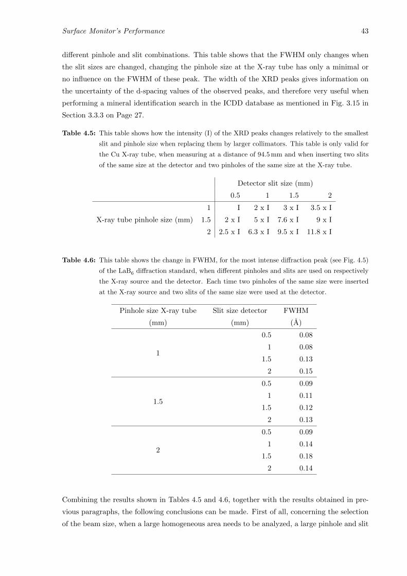
Surface Monitor’s Performance 43
different pinhole and slit combinations. This table shows that the FWHM only changes when
the slit sizes are changed, changing the pinhole size at the X-ray tube has only a minimal or
no influence on the FWHM of these peak. The width of the XRD peaks gives information on
the uncertainty of the d-spacing values of the observed peaks, and therefore very useful when
performing a mineral identification search in the ICDD database as mentioned in Fig. 3.15 in
Section 3.3.3 on Page 27.
Table 4.5: This table shows how the intensity (I) of the XRD peaks changes relatively to the smallest
slit and pinhole size when replacing them by larger collimators. This table is only valid for
the Cu X-ray tube, when measuring at a distance of 94.5 mm and when inserting two slits
of the same size at the detector and two pinholes of the same size at the X-ray tube.
Detector slit size (mm)
0.5 1 1.5 2
X-ray tube pinhole size (mm)
1 I 2 x I 3 x I 3.5 x I
1.5 2 x I 5 x I 7.6 x I 9 x I
2 2.5 x I 6.3 x I 9.5 x I 11.8 x I
Table 4.6: This table shows the change in FWHM, for the most intense diffraction peak (see Fig. 4.5)
of the LaB6 diffraction standard, when different pinholes and slits are used on respectively
the X-ray source and the detector. Each time two pinholes of the same size were inserted
at the X-ray source and two slits of the same size were used at the detector.
Pinhole size X-ray tube
(mm)
Slit size detector
(mm)
FWHM
(A)
1
0.5 0.08
1 0.08
1.5 0.13
2 0.15
1.5
0.5 0.09
1 0.11
1.5 0.12
2 0.13
2
0.5 0.09
1 0.14
1.5 0.18
2 0.14
Combining the results shown in Tables 4.5 and 4.6, together with the results obtained in pre-
vious paragraphs, the following conclusions can be made. First of all, concerning the selection
of the beam size, when a large homogeneous area needs to be analyzed, a large pinhole and slit

44 Results: Characterization and Applications of the Surface Monitor
size is recommended. By using the largest collimators the acquisition time can be shortened to
only 1 s LT/step and the intensity of the diffraction peaks will still be twice more intense when
using the smallest collimators with 5 s LT/step. However, one needs to take into account that
the width of the XRD peaks increases when using larger collimator sizes. In another situation,
when a small area needs to be analyzed it is better to use the smallest pinhole size since this
results in the smallest beam size of 16 mm x 3 mm. This beam size is obtained by measuring
at 95 mm and by varying the tube angle from 12° to 45°. Concerning the slit sizes there are
two options. When a large slit is used, the intensity of peak increases though its width also
broadens. The choice of small slit sizes results in narrower but less intense peaks. To increase
the number of counts, the acquisition time can be increased, but this leads to a longer measur-
ing time. Finally, combining the results from Table 4.5 and Fig. 4.9, due to increased intensity
when choosing larger collimators, better MDLs are obtained.
The performance of the Surface Monitor equipped with the Mo anode X-ray tube was not
investigated due to the lack of time. However, as already explained, it is expected that the
Surface Monitor will best perform when equipped with the Cu anode X-ray source. In the next
section, the results of the very first applications of the Surface Monitor are presented.
4.2 Applications
After the characterization, the methodology of the Surface Monitor was applied to two different
paintings. The primary aim was to identify the pigments used in these works of art. One
painting was provided by the Raman Spectroscopy Research Group and is shown in Fig. 4.15;
this work of art could be investigated in the laboratories of the UGent-XMI Group. The
other painting is the so called “Dulle Griet” or Mad Meg, painted by the Flemish renaissance
artist Pieter Bruegel the Elder in 1561-1562. The painting is currently exhibited at the Museum
Mayer van den Bergh in Antwerp (Belgium). A photo of the “Dulle Griet” is shown in Fig. 4.16.
A few zones were selected from each painting and on each zone a simultaneous XRF/XRD
measurement was performed. The results of these measurements are shown in the next two
sections starting with the painting provided by the Raman Spectroscopy Research Group. All
measurements were performed by using the Cu anode X-ray source (28 kV/250µA).

Applications 45
Figure 4.15: “Colorful flowers in a vase” painted by Perot. This painting that was provided by the
Raman Spectroscopy Research Group and it was investigated in the laboratories of the
UGent-XMI Group. The zone that was analyzed is indicated on the photo.

46 Results: Characterization and Applications of the Surface Monitor
Figure 4.16: “Dulle Griet” or Mad Meg, by Pieter Bruegel the Elder (1561-1562). The painting is
exhibited at the Museum Mayer van den Bergh in Antwerp (Belgium). On this photo the
four zones that were analyzed with the Surface Monitor are indicated. Fig. 4.19 shows
four detailed pictures of these zones.

Applications 47
4.2.1 XRF/XRD Analysis of the Painting “Colorful Flowers in a Vase”
One zone of this painting was analyzed with the Surface Monitor and is indicated on Fig. 4.15.
Details and results of the measurement are summarized in the next paragraph.
The white pigment was characterized using the following acquisition set-up: 2θi of 30° to 2θf
of 90°, step size of 0.2°, 5 s LT/step, two slits of 1.5 mm were used at the detector and two
pinholes of 1.5 mm were inserted at the X-ray tube. The instrument was placed at a distance
of 94.6 mm from the painting. The resulting XRF and XRD spectrum are shown in respectively
Figs. 4.17 and 4.18. The XRF spectrum gives more information about the elements that are
present in the white pigment, these elements are: Ca, Fe, Ba, Zn, Pb and Sr. For the element
Cu it is impossible to determine if it is present in the sample or not because the Cu anode
X-ray source was used. With the information obtained from the XRF spectrum the following
white pigments could be present: BaSO4, ZnO and lead white. To see which of these mineral
phases are actually present in the white pigment, the XRD spectrum is analyzed.
From the XRD spectrum, shown in Fig. 4.18 it is clear that the white pigment consists of the
mineral BaSO4. The other two possible minerals are also added but it is impossible to conclude
that they are also present.
Figure 4.17: XRF spectrum of the lab painting’s white pigment (see Fig. 4.15). The spectrum was
obtained using the Cu anode X-ray source (28 kV/250µA).

48 Results: Characterization and Applications of the Surface Monitor
Figure 4.18: XRD spectrum of the lab painting’s white pigment (see Fig. 4.15). Three mineral phases
are added in the spectrum, the code before the mineral phase can be used to retrieve the
XRD diffraction patterns from the ICDD database.
4.2.2 “Dulle Griet” from Pieter Bruegel the Elder
During the analysis of the “Dulle Griet” with the Surface Monitor four different zones were
measured. These four zones are indicated on Fig. 4.16. Before the start of each measurement
a photo was taken with the webcam, these detailed photos are shown in Fig. 4.19. Practically,
there was a time limit of a one day experiment time (approximately 6 hours in total).
During the measurements the following conditions were applied: 2θi 40°, 2θf 90°, step size 0.2°,
5 s LT/step, two 1.5 mm pinholes were used at the X-ray source and two 0.5 mm slits were used
at the detector. The results, an XRF and XRD spectrum, of the four measurements are shown
below.
Zone 1
The first zone was measured by placing the Surface Monitor at a distance of 94.8 mm. The XRF
and XRD spectra are shown in respectively Fig. 4.20 and Fig. 4.21. From the XRF spectrum
it can be seen that the following elements are present: K, Ca, Mn, Fe, Co and Pb. The copper
K-lines are also visible in the spectrum but since the Cu anode X-ray source was used, it is
impossible to determine if there is Cu present or not. From the XRD spectrum there was only
one mineral phase (CaCO3) found with a good match.
Zone 2
The second zone was measured at a distance of 94.0 mm and the resulting XRF and XRD
spectra are shown in respectively Fig. 4.22 and Fig. 4.23. Seven elements are present in the

Applications 49
XRF spectrum: K, Ca, Mn, Fe, Co, Hg and Pb. The XRD spectrum shows the possible
presence of CaCO3, CaSO4 and the pigment HgO.
(a) Zone 1 (b) Zone 2
(c) Zone 3 (d) Zone 4
Figure 4.19: Detailed photos of the four zones of the “Dulle Griet” that were measured with the
Surface Monitor.
Zone 3
The third zone was measured by placing the instrument at a distance of 94.0 mm. The acquired
XRF and XRD spectra are show in respectively Fig. 4.24 and Fig. 4.25. The XRF spectrum
shows the presence of K, Ca, Mn, Fe and Pb in this zone. The XRD spectrum shows the
possible presence of CaCO3 and CaSO4.
Zone 4
The final zone was measured at a distance of 94.0 mm. The obtained XRF and XRD spectra
are shown in respectively Fig. 4.26 and Fig. 4.27. The XRF spectrum shows the presence of
the following elements: K, Ca, Mn, Fe, Co, Hg and Pb. The XRD spectrum shows the possible
presence of CaCO3 and CaSO4.
From the obtained data it was only possible to determine the mineral phase CaCO3, probably
originating from the preparation layer of the painting. No pigments could be determined
with certainty, due to the complexity of the painting. The painting is in fact a multilayer

50 Results: Characterization and Applications of the Surface Monitor
consisting of different pigment layers and a varnish layer, which makes it hard to find the
different components when the noise level in the XRD spectrum is to high. The relatively large
size of the X-ray beam can also form a problem because adjacent areas colored with other
pigments are irradiated next to the area of interest. For future measurements it should be
considered to measure only one or two points for a longer time to obtain at least one high
quality result instead of measuring as much points as possible, using a shorter measuring time,
resulting in less useful data.
Figure 4.20: XRF spectrum of the first zone of the Dulle Griet painting.
Figure 4.21: XRD spectrum of the first zone of the Dulle Griet painting.

Applications 51
Figure 4.22: XRF spectrum of the second zone of the Dulle Griet painting.
Figure 4.23: XRD spectrum of the second zone of the Dulle Griet painting.

52 Results: Characterization and Applications of the Surface Monitor
Figure 4.24: XRF spectrum of the third zone of the Dulle Griet painting.
Figure 4.25: XRD spectrum of the third zone of the Dulle Griet painting.
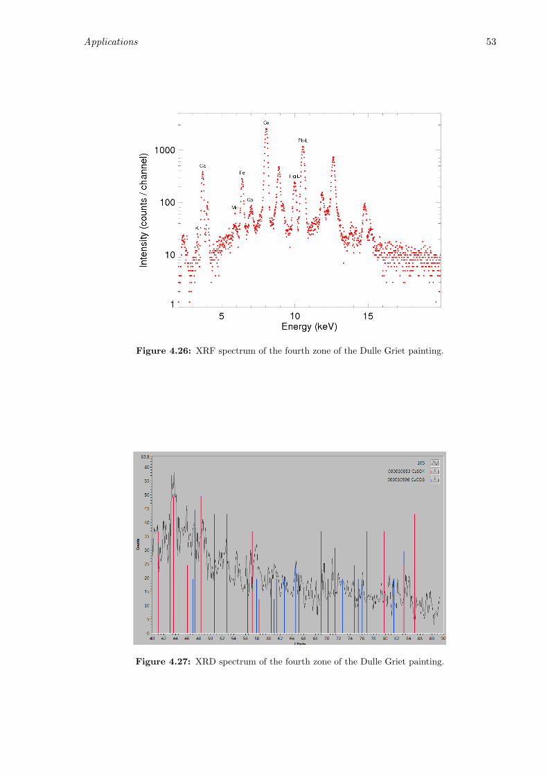
Applications 53
Figure 4.26: XRF spectrum of the fourth zone of the Dulle Griet painting.
Figure 4.27: XRD spectrum of the fourth zone of the Dulle Griet painting.

54 Results: Characterization and Applications of the Surface Monitor

Chapter 5
Summary and Conclusions
The aim of this master thesis was the establishment of the methodology, the characterization
and the application of a novel portable X-ray fluorescence (XRF)/X-ray diffraction (XRD)
instrument, called the Surface Monitor. This instrument was recently acquired by the Ana-
lytical Chemistry Department of the Ghent University (Belgium) from the company Assing
S.p.A. (Rome, Italy). This instrument is described to be used for studying art objects, e.g.
paintings and murals, by combining two powerful non-destructive analytical techniques: X-ray
fluorescence and X-ray diffraction. The success of the XRF methodology is resulting from the
fact that the interaction of X-rays with matter may be fully understood, giving the researcher
a powerful and practical tool to study samples. Where XRF is capable to characterize the ele-
ments present in the sample, XRD gives information about the arrangement of these elements
in the sample, the so called crystal structure. Thus, a combination of these two analysis tech-
niques, XRF and XRD, can be used to obtain a detailed chemical/structural characterization
of the investigated materials.
The main parts of the Surface Monitor are: the X-ray tube (Cu or Mo anode), the X-123 Si-PIN
detector, the laser interferometer and the XRD protractor. All these components are assembled
on the instrument head that is fixed on a tripod. Furthermore, the Surface Monitor is equipped
with a control box, a control portable PC and an extra arm with webcam. This webcam is
not part of the original Surface Monitor as provided by the company Assing S.p.A, but was
added by the UGent-XMI group to improve the safety. The webcam allows the operator to
watch the status of the device head, on a distance, using the control portable PC. Finally, the
manufacturer included collimators in the form of slits and pinholes. These collimators are used
to adjust the beam size and the area analyzed by the detector.
For the acquisition of XRD spectra, the Surface Monitor is equipped with the XRD protractor.
This part ensures the simultaneous movement of the X-ray tube and detector according to
the Bragg-Brentano θ : θ set-up. In order to obtain reliable and reproducible XRD spectra,
the Surface Monitor should be positioned with its main axis perpendicular to the sample’s
surface and at the optimal acquisition distance. The Surface Monitor is positioned at the
55

56 Summary and Conclusions
optimal acquisition distance by using the laser interferometer. The performance, i.e. the
precision, of the laser interferometer was a first point of concern during the characterization
of the Surface Monitor. The precision of the laser was tested by moving a flat surface with a
manual translational stage over certain range. A precision of ±0.11 mm was obtained from the
results, which is sufficient for further applications. Beside the laser interferometer’s precision,
the optimal distance for the acquisition of XRF/XRD spectra was determined. When the
Surface Monitor was delivered, the distance to acquire XRF and XRD spectra was set by
the manufacturer between 91.8 mm and 92.2 mm. During the first tests with the instrument
it became clear that this was not the optimal distance for the acquisition of XRF and XRD
spectra. Therefore a new range was defined by performing XRD measurements with the LaB6
diffraction standard at different distances. From the obtained data it is now recommended to
place the instrument at a distance between 94.5 mm and 95.0 mm from the object to obtain
reliable XRD spectra.
The next step in the Surface Monitor’s characterization was the determination of the beam
size and more importantly the position of the X-ray beam with respect to the footprint of the
laser interferometer beam. The X-ray beam can be collimated by inserting different collimator
sizes at the X-ray source. During the measurements only pairs of collimators of the same size
were used to regulate the size of the X-ray beam. From the obtained results it is recommended
to use the pinhole collimators, since the beam size obtained with the slits is to large for many
further applications. Next to the size of the beam, the position of the beam with respect to the
laser interferometer has also been determined. When the instrument is positioned at a distance
of 95 mm, the laser interferometer is indicating the center of the X-ray beam, which gives an
extra indication that the object must be placed at this distance.
Once the position of the beam and its size on the sample were known with high accuracy, the
minimum detection limits for certain detectable elements could be determined and compared to
other state-of-the-art instrumentation: the EDAX Eagle III micro-XRF spectrometer and the
Olympus Innov-X DELTA handheld XRF analyzer. Minimum detection limits were obtained by
using the NIST SRM 1412 multicomponent glass standard. The resulting minimum detection
limits for the Surface Monitor are between 100 ppm and 3000 ppm, depending on the atomic
number of the detected element, which are approximately one magnitude higher than the
minimum detection limits obtained with the EDAX Eagle III micro-XRF spectrometer and
the Olympus Innov-X DELTA handheld XRF analyzer. This difference is mainly due to the
large distance between the Surface Monitor and the object that was analyzed. By measuring
at a larger distance there is a long air-path between the X-ray source and the sample, and
between the sample and the detector. The large detector distance also reduces considerably the
detection solid-angle, which has a negative influence on the minimum detection limit. In case of
the Olympus Innov-X DELTA handheld XRF analyzer, there are less geometrical constraints
so that the probe head can be placed at a much smaller distance from the sample’s surface.
Executing experiments with the EDAX Eagle III micro-XRF spectrometer, all instrumental

57
parameters are optimized in order to acquire data in optimal conditions.
The last step in characterizing the portable XRF/XRD instrument dealt with the influence
of changing the collimator sizes, at both X-ray source and detector, on the quality of the
XRD spectra. The results were obtained by acquiring XRD spectra of the LaB6 diffraction
standard while using different combinations of slits and pinholes at respectively the detector
and the X-ray source. From the results we can conclude that it is better to use the largest
collimators when measuring a large homogeneous surface, this reduces the measuring time
but also increases the width of the diffraction peaks in the XRD spectrum. For small areas,
the collimators with the smallest opening are recommended but the measuring time must be
sufficiently long to obtain good results. The measurements provided very useful information in
selecting the correct collimators before starting an XRD measurement. This information will
allow future operators of the Surface Monitor to make fast decisions when measuring on the
field.
The final part of this master thesis dealt with the analysis of two paintings: “Colorful flowers
in a vase” by Perot and the famous “Dulle Griet” by Pieter Bruegel the Elder (1561-1562). The
first painting was provided by the Raman Spectroscopy Research Group and it was available at
the laboratory of UGent-XMI Group. One zone, consisting of a white pigment, was analyzed by
the Surface Monitor and the presence of the pigment BaSO4 was demonstrated. The analysis
of the “Dulle Griet” at the Mayer van den Bergh museum in Antwerp (Belgium), was the first
application of the Surface Monitor on the field. Due to a limited amount of time (approximately
6 hours in total) only four measurements were performed on the painting. From the obtained
data it was only possible to determine the mineral phase CaCO3, probably originating from
the preparation layer of the painting. No pigments could be determined with certainty, due
to the complexity of the painting. The painting is in fact a multilayer consisting of different
pigment layers and a varnish layer, which makes it hard to find the different components when
the noise level in the XRD spectrum is to high. The relatively large size of the X-ray beam can
also form a problem because adjacent areas colored with other pigments are irradiated next to
the area of interest. For future measurements it should be considered to measure only one or
two points for a longer time to obtain at least one high quality result instead of measuring as
much points as possible, using a shorter measuring time, resulting in less useful data.
Finally, it should be mentioned that the Surface Monitor is still under development and can
still be improved in some ways. The detection of X-rays can be improved by using a Silicon
Drift Detector (SDD) instead of the Si-PIN detector. The SDD has a lower dead time and
higher resolution compared to the Si-PIN detector that is now used by the Surface Monitor.
The Cu anode X-ray source can be changed by the Mo anode X-ray source, but this is only
improving the quality of the XRF spectra. For XRD measurements it is recommended to use
the Cu anode X-ray tube. The geometry of the XRD protractor can be changed to decrease the
optimal distance between the probe head and the sample. If this distance could be decreased,

58 Summary and Conclusions
the detector and the X-ray source are positioned at a closer distance towards the sample’s
surface which improves the count rate.

Appendix A
Standard Reference Material
A.1 NIST SRM 1412 Multicomponent Glass Standard
The NIST SRM 1412 multicomponent glass standard was used to determine the minimum
detection limits for the Surface Monitor and to compare them with two other instruments: the
EDAX Eagle III micro-XRF spectrometer and the Olympus Innov-X DELTA handheld XRF
analyzer. The certified mass fractions of this standard are shown in Table A.1.
Table A.1: Certified concentrations for the NIST SRM 1412 multicomponent glass standard. Repro-
duced from NIST SRM 1412 certificate [32].
Element Mass fraction (ppm) Element Mass fraction (ppm)
Si 198074 Li 20904
Al 39798 B 14068
Ca 32376 Ba 41827
Mg 28280 Zn 35992
Sr 38474 Pb 40846
Na 34797 Cd 38342
K 34368 Fe 217
A.2 NIST SRM 660b Diffraction Standard
The NIST SRM 660b diffraction standard was used to optimize the Surface Monitor’s XRD
acquisition mode. The standard was used e.g. to determine the ideal range for XRD acquisition,
to determine the offset of the diffraction peaks, and to study the consequences of using different
slit and pinhole sizes on respectively the detector and the Cu anode X-ray tube. A unit of the
SRM 660b consists of approximately 6 g of lanthanum hexaboride (LaB6) powder bottled under
argon. Before one can start measuring the LaB6-powder it is necessary to bring the powder
in a stable formulation so that there is no loss of the material during transport or during the
analysis and to prevent contamination with other crystalline materials. Therefore, a sufficient
59

60 Standard Reference Material
amount of the LaB6-powder is placed between two layers of 4µm Ultralene® Window Film
(purchased from SPEX CertiPrep Group) and fixed on an 31 mm Double Open-Ended X-Cell
(purchased from SPEX CertiPrep Group). The result is shown in Fig. A.1. Since the polymer
used for the manufacturing of the Ultralene® Window Film also gives rise to diffraction peaks,
a second sample was made without the NIST SRM 660b. From both samples, one with the
diffraction standard and one without diffraction standard, an XRD spectrum was record and
shown in Fig. A.2. By comparing both spectra in Fig. A.2 one can see that the peaks at 17.4°
and 25.6° are originating from the Ultralene® film. The information values for peak positions
between 20° and 90° for the NIST SRM 660b are shown in Table A.2.
Figure A.1: NIST SRM 660b (LaB6) diffraction standard placed between two layers of Ultralene® and
fixed on a Double Open-Ended X-Cell that can be stored in a box for easy transportation.
(a) (b)
Figure A.2: Diffraction spectra of the Ultralene® Window Film (a) with and (b) without the NIST
SRM 660b diffraction standard.

NIST SRM 660b Diffraction Standard 61
Table A.2: Information values for peak positions computed for the NIST SRM 660b, using the Cu-Kα
radiation. Only the values between 20° and 90° 2θ are shown. Reproduced from NIST
SRM 660b certificate [32].
h k l 2θ (°) h k l 2θ (°)
1 0 0 21.358 3 0 0 67.548
1 1 0 30.385 3 1 0 71.746
1 1 1 37.442 3 1 1 75.844
2 0 0 43.507 2 2 2 79.870
2 1 0 48.958 3 2 0 83.846
2 1 1 53.989 3 2 1 87.792
2 2 0 63.219

62 Standard Reference Material

Appendix B
Flo2spe-Converter
The program flo2spe-converter can be used to convert the flo output files, generated by the
Surface Monitor’s software package, into spe files. The flo output file contains all information
concerning an XRF acquisition such as: tube voltage and current, detector and tube angles,
measuring time, etc. Next to this information it also contains the number of counts per channel.
The number of counts per channel will be extracted from the flo file and written in a new spe
file by the program flo2spe-converter. This spe file can be used to process the obtained XRF
spectrum by the AXIL software package. The program flo2spe-converter was written in the C
language on a CentOS (release 6.1) operating system and compiled with gcc (version 4.4.5).
The source code is given below.
Source code flo2spe-converter
1 // Program to convert flo to spe
// Written by Robin De Wolf during Master Thesis (2011-2012)
3
#include<stdio.h>
5 #include<stdlib.h>
#include<stdbool.h>
7 #include<string.h>
9 #define CHANNELS 2048 /*Change channel number here if necessary*/
11 int main (int argc, char *argv[]) {
int fileCount;
13 int buffer[CHANNELS];
15 bool ReadFlo (char *inputfile, int output[CHANNELS]);
bool MakeSpe (char *inputfile, const int counts[], const int channels);
17
if (argc == 1) { /*Check if there is at least 1 input file*/
19 printf ("Need one or more .flo files!\n");
return EXIT_FAILURE; }
21
63
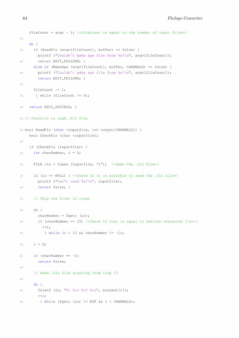
64 Flo2spe-Converter
fileCount = argc - 1; /*fileCount is equal to the number of input files*/
23
do {
25 if (ReadFlo (argv[fileCount], buffer) == false) {
printf ("Couldn’t make spe file from %s!\n", argv[fileCount]);
27 return EXIT_FAILURE; }
else if (MakeSpe (argv[fileCount], buffer, CHANNELS) == false) {
29 printf ("Couldn’t make spe file from %s!\n", argv[fileCount]);
return EXIT_FAILURE; }
31
fileCount -= 1;
33 } while (fileCount != 0);
35 return EXIT_SUCCESS; }
37 // Function to read .flo file
39 bool ReadFlo (char *inputfile, int output[CHANNELS]) {
bool CheckFlo (char *inputfile);
41
if (CheckFlo (inputfile)) {
43 int charNumber, i = 0;
45 FILE *in = fopen (inputfile, "r"); /*Open the .flo file*/
47 if (in == NULL) { /*Check if it is possible to read the .flo file*/
printf ("Can’t read %s!\n", inputfile);
49 return false; }
51 // Skip the first 12 lines
53 do {
charNumber = fgetc (in);
55 if (charNumber == 10) /*Check if char is equal to newline character (\n)*/
++i;
57 } while (i < 12 && charNumber != -1);
59 i = 0;
61 if (charNumber == -1)
return false;
63
// Read .flo file starting from line 13
65
do {
67 fscanf (in, "%i %*c %*f %*c", &output[i]);
++i;
69 } while (fgetc (in) != EOF && i < CHANNELS);

65
71 fclose (in); /*Close flo file*/
73 return true; }
75 return false; }
77 // Function to check flo file
79 bool CheckFlo (char *inputfile) {
if (strstr (inputfile, ".flo") != NULL)
81 return true;
else {
83 printf("%s isn’t a correct flo file!\n", inputfile);
return false; } }
85
// Function to create the .spe file
87
bool MakeSpe (char *inputfile, const int counts[], const int channels) {
89 char *outputfile;
int i;
91
void NewName (char *old, char *new);
93
// Allocate memory to pointer
95
if ((outputfile = (char *) malloc ((strlen (inputfile) + 1) * sizeof (char))) ==
NULL) { /*strlen doesn’t count the terminating ’\0’, therefore the +1 is
inserted*/
97 printf("Memory allocation error!");
return false; }
99
// Create file name
101
NewName (inputfile, outputfile);
103
// Open the new .spe file
105
FILE *out = fopen (outputfile, "w");
107
if (out == NULL) {
109 printf("Can’t write %s!\n", outputfile);
return false; }
111
// Layout .spe file
113
fprintf(out, "$DATA:\n");
115 fprintf(out, "1 %i\n", channels);
117 // Print data to .spe file

66 Flo2spe-Converter
119 for (i = 0; i < channels; ++i) {
fprintf(out, "%i\n", counts[i]); }
121
// Close .spe file
123
fclose (out);
125
// Free the allocated memory
127
free (outputfile);
129
return true; }
131
// Function to create a name for the new .spe file
133
void NewName (char *old, char *new) {
135 char *p;
137 p = strchr (old, ’.’);
strcpy(new, old);
139 strcpy (new + (p - old), ".spe"); }
flo2spe.c

Bibliography
[1] Assing S.p.A. (2011). Adress: Via E. Amaldi 14 - Monterotondo (Italy). URL http:
//www.assing-group.it/index_eng.html.
[2] B. Beckhoff, N. Langhoff, B. Kanngiefer, R. Wedell & H. Wolff, eds. (2006). Handbook of
Practical X-Ray Fluorescence Analysis. Springer Verlag, Berlin.
[3] L. Vincze (2011). Advanced Spectroscopic Methods of Analysis. Course Master Chemistry,
Ghent University 2011-2012.
[4] Nobelprize.org (2011). Wilhelm Conrad Rontgen. URL http://www.nobelprize.
org/nobel_prizes/physics/laureates/1901/rontgen-bio.html.
[5] Amptek (2011). X-ray Fluorescence Spectroscopy. URL http://www.amptek.com.
[6] D. Depla (2009). Kristalchemie, Een inleiding op X-straaldiffractie. Course Bachelor
Chemistry, Ghent University 2009-2010.
[7] P. Jeffrey (2012). X-ray Data Collection Course. URL http://xray0.princeton.
edu/˜phil/Facility/Guides/XrayDataCollection.html.
[8] C. Suryanarayana & M. Grant Norton, eds. (1998). X-Ray diffraction: a practical ap-
proach. Plenum Press, New York.
[9] Wikipedia (2011). Thomson Scattering. URL http://en.wikipedia.org/wiki/
Thomson_scattering.
[10] C. Hammond, ed. (2009). The Basics of Crystallography and Diffraction. Oxford Univer-
sity Press Inc., New York, third edit ed.
[11] Wikipedia (2011). Bragg’s law. URL http://en.wikipedia.org/wiki/Bragg’s_
law.
[12] Wikipedia (2011). X-ray tube. URL http://en.wikipedia.org/wiki/X-ray_
tube.
[13] J. K. Cockcroft (2011). Generation of X-rays. URL http://pd.chem.ucl.ac.uk/
pdnn/inst1/xrays.htm.
67

68 Bibliography
[14] P. J. Goodhew, J. Humphreys & R. Beanland, eds. (2001). Electron Microscopy and
Analysis. Taylor & Francis, London, third ed.
[15] M. Azadeh, ed. (2009). Fiber Optics Engineering. Optical Networks. Springer US, Boston,
MA, 1 ed.
[16] Assing (2011). Assing Surface Monitor User’s Manual.
[17] D. Blake & C. Bryson (1992). Design of an x-ray diffraction/x-ray fluorescence instrument
for planetary applications. Lunar and Planetary Institute, 13:117–118.
[18] D. Blake, C. Bryson & F. Freund (1993). X-ray diffraction apparatus, U.S. Pattent No.
5,491,738.
[19] S. Cornaby, A. Reyes-Mena, H. K. Pew, P. W. Moody, T. Hughes, A. Stradling, D. C.
Turner & L. V. Knight (2001). An XRD/XRF instrument for the microanalysis of rocks
and minerals. Measurement Science and Technology, 12(6):676–683.
[20] S. Cornaby, A. Reyes-Mena, P. Moody, A. Stradling, T. Grow & L. Knight (2002). Simul-
taneous XRD/XRF with Low-Power X-ray Tubes. Adv. in X-ray Analysis, 45(c):34.
[21] M. Uda (2004). In situ characterization of ancient plaster and pigments on tomb walls
in Egypt using energy dispersive X-ray diffraction and fluorescence. Nuclear Instruments
and Methods in Physics Research Section B: Beam Interactions with Materials and Atoms,
226(1-2):75–82.
[22] M. Uda, A. Ishizaki, R. Satoh, K. Okada, Y. Nakajima, D. Yamashita, K. Ohashi,
Y. Sakuraba, A. Shimono & D. Kojima (2005). Portable X-ray diffractometer equipped
with XRF for archaeometry. Nuclear Instruments and Methods in Physics Research Section
B: Beam Interactions with Materials and Atoms, 239(1-2):77–84.
[23] A. Gianoncelli, J. Castaing, L. Ortega, E. Dooryhee, J. Salomon, P. Walter, J. Hodeau
& P. Bordet (2008). A portable instrument for in situ determination of the chemical and
phase compositions of cultural heritage objects. X-Ray Spectrometry, 37(4):418–423.
[24] A. Duran, J. Perez-Rodriguez, M. Jimenez de Haro, M. Franquelo & M. Robador (2011).
Analytical study of Roman and Arabic wall paintings in the Patio De Banderas of Reales
Alcazares’ Palace using non-destructive XRD/XRF and complementary techniques. Jour-
nal of Archaeological Science, 38(9):2366–2377.
[25] S. Pages-Camagna, E. Laval, D. Vigears & A. Duran (2010). Non-destructive and in situ
analysis of Egyptian wall paintings by X-ray diffraction and X-ray fluorescence portable
systems. Applied Physics A, 100(3):671–681.
[26] A. Pifferi, G. Campi, C. Giacovazzo & E. Gobbi (2009). A new portable XRD/XRF
instrument for non-destructive analysis. Croatica Chemica Acta, 82(2):449–454.

Bibliography 69
[27] Amptek Inc. (2012). Adress: De Angelo Drive 14 - Bedford (U.S.A.). URL http://www.
amptek.com.
[28] B. Vekemans, K. Janssens, L. Vincze, F. Adams & P. Van Espen (1994). Analysis of
X-ray spectra by iterative least squares (AXIL): New developments. X-Ray Spectrometry,
23(6):278–285.
[29] B. De Samber (2010). Spatially resolved X-ray micro/nano-spectroscopy and imaging on the
model organism Daphnia magna using laboratory and synchrotron sources. Ph.D. thesis,
Ghent University.
[30] International Center for Diffraction Data (2012). Adress: Campus Boulevard 12 - Newtown
Square (U.S.A.). URL http://www.icdd.com/.
[31] NIST (2012). Measures of Skewness and Kurtosis. URL http://www.itl.nist.gov/
div898/handbook/eda/section3/eda35b.htm.
[32] NIST (2012). Standard Reference Materials. URL http://www.nist.gov/srm/
index.cfm.

70 Bibliography

Ingebruikname, Analytische Karakterisering en Toepassing vaneen Nieuw Draagbaar XRF/XRD Instrument
Robin De Wolfa,∗, Bart Vekemansa, en Laszlo Vinczea
aX-Ray Microspectroscopy and Imaging Group (XMI), Department of AnalyticalChemistry, Ghent University, Krijgslaan 281, S12, B-9000 Ghent, Belgium
∗E-mail: [email protected]
De Surface Monitor, i.e. een draagbaar X-straal fluorescentie (XRF)/X-straal diffractie (XRD) instrument, werd in 2011 aangekocht bij de firmaAssing S.p.A (Rome, Italie) door de Vakgroep Analytische Chemie van deGentse Universiteit (Belgie). Vooraleer dit toestel kan worden toegepastom metingen uit te voeren op kunstobjecten werden verschillende aspectenvan de Surface Monitor getest. Dit houdt in: het bepalen van de laserinterferometer’s betrouwbaarheid, het bepalen van de optimale XRF/XRDmeetafstand, het bepalen van de bundelgrootte en de positie van de X-straalten opzichte van de laser interferometer, bepalen van de minimum detectielimieten voor XRF, en tenslotte de invloed onderzoeken van collimatorenop XRD spectra. De Surface Monitor werd voor de eerste keer getesttijdens de karakterisatie van het schilderij de “Dulle Griet” in het museumMayer van den Bergh in Antwerpen (Belgie).
Trefwoorden: draagbaar, XRF, XRD, Surface Monitor
Inleiding
De analyse van kostbare kunstobjecten is een moeilijke onderneming omdat het meestal on-mogelijk is om stalen te nemen van deze kostbare voorwerpen, en deze objecten kunnen nietaltijd naar een laboratorium gebracht worden om te worden geanalyseerd met niet-destructieveanalytische technieken. Daarom werd er de laatste jaren geınvesteerd in onderzoek naar draag-bare XRF/XRD systemen welke het mogelijk maken de kunstobjecten ter plaatse, bv. in eenmuseum, te gaan analyseren. Hieronder volgt een kort overzicht.
In het NASA (National Aeronautics and Space Administration) Ames Research Center werdin 1992 het eerste prototype van een XRF/XRD instrument ontwikkeld [1, 2]. Dit instrumentcombineert twee krachtige niet-destructieve analytische technieken nl. XRF en XRD. XRFwordt ingezet om al een eerste indicatie te geven van de aanwezige mineralen, aan de handvan de elementaire samenstelling van het monster. De definitieve identificatie van de aan-wezige mineralen is met behulp van XRD. Het uiteindelijke toestel zou worden gebruikt voorplanetaire exploratie en als een draagbaar instrument voor het analyseren van kunst objecten.In 2000 werd er door MOXTEK, Inc. een poging ondernomen om een draagbaar XRF/XRDinstrument te ontwikkelen [3]. Figuur 1a toont een foto van deze opstelling, met de bijhorendecomponenten. De CCD (charged-coupled device) detector kan gezien worden als een van debelangrijkste onderdelen van dit toestel. Deze detector maakt het immers mogelijk om ge-lijktijdig zowel een XRF als een XRD spectrum op te nemen. Met behulp van een softwarealgoritme worden de XRF en de XRD data van elkaar gescheiden. Het grootste nadeel aan ditinstrument is de grote X-stralen buis, maar deze zal voor later toepassingen worden vervangendoor een laag vermogen X-stralen buis. Naast de te grote X-stralen buis is er ook nog de CCDdetector waarvan de resolutie te laag is om bepaalde diffractie pieken van elkaar te kunnenonderscheiden.
71

In 2004 combineerde Uda [4] een laag vermogen X-stralen buis met een Si-PIN detector ineen draagbare energie dispersieve X-straal diffractie en fluorescentie (ED-XRDF) spectrome-ter. Deze combinatie had vele voordelen: kleine dimensie, licht gewicht, korte meettijd, niet-destructieve en contact vrije meting, geen restricties met betrekking tot de vorm en grote vanhet monster, er is geen speciale koeling nodig, en het toestel wordt bestuurd met behulp van eencomputer. Het toestel werd gebruikt om op archeologische sites de samenstelling van pigmentente bepalen. Desondanks de vele voordelen van dit instrument is het nog steeds moeilijk omde samenstelling van complexe pigmenten te bepalen door een te hoge achtergrond en minderintense pieken in het diffractie spectrum [5].
Een nieuw XRF/XRD instrument werd in 2007 ontwikkeld door Gianoncelli et. al [5]. Figuur 1btoont een foto van dit instrument. Dit toestel bestaat uit een koper anode X-stralen buis (rechtsop de foto), een silicon drift XRF detector (centraal op de foto) en een imaging plate (links opde foto). Alle onderdelen zijn bevestigd op een frame wat het mogelijk maakt om te bewegenlangsheen het oppervlak van het te analyseren object. Belangrijkste nadeel aan dit instrumentis de reproduceerbaarheid van de XRD resultaten: 1 mm afwijken van het referentie punt zorgtal voor een afwijking van 3° in het XRD spectrum.
In 2008 werd door de firma Assing S.p.A. (Rome, Italie) een compact instrument ontwikkeldwaarmee het mogelijk was gelijktijdig XRF en XRD metingen uit te voeren [6]. Volgens Pifferiet. al [7] waren de resultaten, bekomen met dit nieuwe toestel nog steeds onbetrouwbaar door demechanische instabiliteit. Om deze problemen te overkomen werd het prototype aangepast meteen koper anode X-stralen buis, een silicon solid state detector en een horizontale Theta-Thetagoniometer (zie Figuur 1c). Met behulp van een laser interferometer wordt het instrument opde juiste afstand van het te analyseren object geplaatst en het toestel kan in drie verschillendemodi worden gebruikt: een XRF, een XRD en een XRF/XRD modus. De laatste modus houdtin dat tegelijkertijd een XRF en XRD spectrum kan worden opgenomen. Verder maakt dehardware het mogelijk dat de X-stralen buis en de detector symmetrisch over een interval van10° < 2θ < 140° kunnen bewegen.
(a) XRF/XRD instrument ontwikkeld doorMOXTEK, Inc. gebruikt door Cornabyet. al [3].
(b) XRF/XRD instrument gebruikt doorGianoncelli et al. [5].
(c) XRF/XRD instrument gebruikt doorPifferi et al. [7].
Figuur 1: Foto’s van XRF/XRD instrumenten beschreven in de literatuur.
72

In 2011 werd de Surface Monitor aangekocht door de Vakgroep Analytische Chemie van deGentse Universiteit. De beschrijving van de componenten van dit toestel en de bijhorendedataverwerking worden beschreven in het volgende deel van dit werk.
Beschrijving van de Surface Monitor
De Surface Monitor van Assing S.p.A (model 2011-2012) bestaat uit de volgende onderdelen:een meetkop, een statief, een controle box, een laptop en een extra arm met een webcamera.De webcamera werd door de UGent-XMI groep aan de Surface Monitor toegevoegd om deveiligheid te bevorderen. De webcamera zorgt ervoor dat de operator vanop afstand de statusvan de Surface Monitor kan controleren met behulp van de laptop. Figuur 2a toont de volledigeopstelling van de Surface Monitor: de bovenvermelde meetkop is gemonteerd op een statief enverbonden met de controle box met de nodige elektronica, de besturing gebeurt met behulp vande laptop. De webcamera is niet te zien op deze foto, maar wordt bevestigd aan de horizontalearm van het statief en wordt naar de meetkop gericht. Figuur 2b toont een bovenaanzicht vande meetkop met de belangrijkste onderdelen: X-stralen buis, X-123 Si-PIN detector en tusseninde laser interferometer.
(a) Opstelling Surface Monitor (b) Meetkop (c) Collimatoren
Figuur 2: Foto’s van (a) de opstelling van de Surface Monitor volgens het veiligheidshandboek (1,laptop; 2, controle box; 3, meetkop; 4, statief), (b) bovenaanzicht van de meetkop en (c)beschikbare collimatoren (links: pinholes gebruikt voor de X-stralen buis; rechts: verticaleslits gebruikt voor de detector); de collimatoren worden steeds in paren gebruikt.
Twee X-stralen buizen zijn beschikbaar om metingen met de Surface Monitor uit te voeren:een koper anode en een molybdeen anode X-stralen buis. Enkel de koper anode werd gebruikttijdens het uitvoeren van de experimenten omdat deze X-stralen buis de beste resultaten geeftop vlak van XRD in vergelijking met de molybdeen X-stralen buis. De maximale spanning enstroomsterkte op de koper anode bedragen respectievelijk 30 kV en 500µA. Tijdens de me-tingen werd er telkens een spanning van 28 kV en een stroomsterkte van 250µA aangebrachtop de koper anode X-stralen buis. Verder dient nog te worden opgemerkt dat beide X-stralenbuizen niet uitgerust zijn met een monochromator. Voor de detectie van X-stralen is de Sur-face Monitor uitgerust met een X-123 Si-PIN detector van de firma Amptek Inc. [8]. Beideonderdelen, X-stralen buis en detector, kunnen voorzien worden van collimatoren met verschil-lende diameter of met een varierende breedte. De beschikbare collimatoren zijn weergegevenin Figuur 2c. De pinhole diameters zijn, van bovenaan te beginnen, ongeveer 0, 5 mm, 1 mm,1, 5 mm en 2 mm. De breedte van de verticale slits zijn, van bovenaan te beginnen, ongeveer0, 5 mm, 1 mm, 1, 5 mm en 2 mm, de lengte van elke slit is ongeveer gelijk aan 8 mm. De colli-matoren kunnen in de voorziene ruimtes van de X-stralen buis en detector worden geschovenen ze worden gefixeerd met behulp van schroeven. Deze schroeven worden tijdens de metingenverwijderd om te voorkomen dat deze het te analyseren object zouden beschadigen en om decollimatoren handig te kunnen verwisselen tussen twee metingen door. De keuze van het type
73

collimatoren heeft een belangrijke invloed op de XRD spectra. Indien een collimator met eenkleine opening wordt gekozen, worden de pieken in het XRD spectrum smaller en de resolutiehoger. Daartegenover staat dat het instrument zeer precies moet worden gepositioneerd. Tij-dens de metingen werden paren van pinholes enkel gebruikt voor de X-stralen buis en parenvan verticale slits voor de detector. Het volgende onderdeel van de Surface Monitor, is de laserinterferometer. Dit onderdeel wordt gebruikt om de Surface Monitor op de optimale afstandvan het te analyseren object te plaatsen, wat belangrijk is om betrouwbare en reproduceerbareXRD spectra te bekomen. Tenslotte is er nog de XRD protractor. Dit onderdeel zorgt voorde simultane beweging van de X-stralen buis en de detector tijdens een XRD meting, volgensde Bragg-Brentano θ : θ methode. Deze meetmethode houdt ook in dat de afstand tussen deX-stralen buis en het staal, en tussen de detector en het staal identiek moeten zijn om be-trouwbare resultaten te bekomen. In de praktijk is het bereik van de detector en de X-stralenbuis beperkt omdat deze bij kleine hoeken het te analyseren object kunnen raken.
Dataverwerking
De evaluatie van de XRF spectra werd uitgevoerd met behulp van het AXIL softwarepakket [9]. Deze software werd onder andere gebruikt voor het bepalen van de karakteristiekefluorescentie lijnen, sompieken, escape pieken, enz. Eens de spectrum evaluatie is afgerond,kan met behulp van de netto piek oppervlakten bv. de minimum detectie limieten berekendworden.
De interpretatie van de XRD spectra werd uitgevoerd via het programma “XRD match!”,dat behoort tot het software pakket van de Surface Monitor. De interpretatie van de XRDspectra is gebaseerd op het vergelijken van de bekomen diffractie pieken met gegevens uit eendatabase. Voor dit werk werd een database van het International Center for Diffraction Data(ICDD) (PDF-4/minerals 2010 relational database; version 4.1011) gebruikt [10]. Vooraleer hetbekomen spectrum kan vergeleken worden met de gegevens uit de database dient de gebruikereerst een aanduiding te geven van de aanwezige elementen (deze informatie wordt bekomen uithet XRF spectrum) en moeten de verschillende diffractie pieken geselecteerd worden. Hieruitvolgt een lijst met mineralen die mogelijk aanwezig zijn in het staal. De XRD spectra van dezemineralen worden vervolgens vergeleken met het experimenteel bekomen XRD spectrum tot ereen match wordt gevonden.
Experimenteel
Zoals reeds vermeld speelt de laser interferometer een cruciale rol in het positioneren van deSurface Monitor voor het te analyseren object. Omdat dit zo een belangrijk onderdeel is, werdbepaald hoe precies de afstandsmeting gebeurt. Hiervoor werd de laser loodrecht op een vlakoppervlak gericht, i.e een stuk papier geplakt op een houder dat op zijn beurt op een “manualtranslational stage” (Standa; type 7T184-13) werd geplaatst. De “manual translational stage”had een afleesnauwkeurigheid van 0, 005 mm. Het oppervlak werd verschoven met stappen van0, 050 mm over een afstand van 10 mm.
Naast de prestaties van de laser interferometer werd de optimale XRF/XRD meetafstandbepaald. Toen het toestel werd afgeleverd, werd aangeraden door de firma Assing S.p.A. om deobjecten op een afstand tussen de 91, 8 mm en 92, 2 mm te plaatsen. Uit de eerste metingen opdeze afstand bleek echter dat dit niet de optimale afstand kon zijn. Om een nieuwe optimaleafstand te definieren werd de NIST SRM 660b diffractie standaard gebruikt. Deze standaardwerd op verschillende afstanden van de Surface Monitor gemeten. Telkens werd het aantaltellen van de meest intense diffractie piek genoteerd en de afwijking van deze piek ten opzichtevan de gecertificeerde 2θ-waarde, i.e. 30,385°. Volgende parameters werden gebruikt voor deXRD meting: de meting starte bij 2θi van 15° tot een 2θf van 90° met stappen van 0,2°, en elkestap werd gedurende 5 s LT (live time) gemeten. Twee pinholes van 1 mm werden gebruikt bijde X-stralen buis en twee verticale slits van 1 mm werden gebruikt bij de detector.
Verder werd ook nog de bundelgrootte van de X-straal bepaald. Om de bundelgrootte te
74

bepalen, werden dezelfde omstandigheden gebruikt als tijdens een XRF/XRD meting. DeX-stralen buis bewoog van 12° tot en met 45° met stappen van 0,1° en een meettijd van5 s LT/stap. Via deze opstelling werden twee metingen uitgevoerd. Voor de eerste metingwerden twee pinholes met een diameter van 1 mm gebruikt en voor de tweede meting werdentwee pinholes van 1, 5 mm gebruikt. De bundelgrootte werd bepaald met behulp van een zelfontwikkelende GAFChromic® (type: RQTA2) film, welke op een afstand van 95 mm werdgeplaatst.
De volgende stap in de karakterisatie van de Surface Monitor was het bepalen van de minimumdetectie limieten (MDL). De MDL is de concentratie van een bepaald element die nodig is omde piek van dit element te onderscheiden van de achtergrond. De MDL werden bepaald metde NIST SRM 1412 glas standaard en met behulp van volgende formule:
CMDL,i =3√NB,i
NN,i× Ci (1)
met CMDL,i de minimum detectie limiet voor element i, NB,i het aantal tellen van de achter-grond, NN,i het netto aantal tellen van element i en Ci de concentratie van element i in destandaard. De MDL voor de Surface Monitor werden bepaald door gebruik te maken van drieverschillende collimator combinaties. Twee verticale slits (detector) van 2 mm, 1, 5 mm en 1 mmwerden gecombineerd met respectievelijk twee pinholes (X-stralen buis) van 2 mm, 1, 5 mm en1 mm. Elke combinatie werd gedurende 1000 s LT gemeten op een afstand van 95, 0 mm. Tervergelijking werden de MDL nog bepaald voor volgende state of the art toestellen: EDAX Ea-gle III micro-XRF spectrometer en de Olympus Innov-X DELTA handheld XRF analyzer. DeEDAX Eagle III is een laboratorium instrument bestaande uit een rhodium anode X-stralenbuis en polycapillaire optica. Het tweede toestel bestaat ook uit een rhodium anode X-stralenbuis met een bundelgrootte van 5 mm, dit toestel is geoptimaliseerd om op verplaatsing tegebruiken. De NIST SRM 1412 werd met de EDAX Eagle III op vier verschillende puntengemeten voor 250 s/punt en dit zowel onder vacuum als in lucht. De vier spectra werdentelkens gecombineerd zodat een somspectrum van 1000 s werd bekomen om hieruit dan deMDL te berekenen. De NIST SRM 1412 werd met de handheld XRF analyzer in totaal 300 sgemeten en de resultaten werden herleid naar een meting van 1000 s om te kunnen vergelijkenmet de resultaten van de Surface Monitor en de EDAX Eagle III.
Tenslotte werd nog de invloed van verschillend collimatoren op een XRD spectrum nagegaan.Deze informatie is van belang tijdens metingen op locatie, bv. in een museum. Tijdens dezemetingen wordt de gebruiker geconfronteerd met een zeker tijdsdruk, daarom is het nuttigom de invloed van de verschillende pinholes en slits op het XRD spectrum na te gaan enhoe de kwaliteit kan verbeterd worden door andere combinaties te gebruiken. Het effect vande collimatoren werd getest met behulp van de NIST SRM 660b diffractie standaard. Destandaard werd telkens op een afstand van 94, 5 mm geplaatst en de meting startte bij eenhoek van 15° 2θ tot 90° 2θ met stappen van 0,2° en een meettijd van 5 s LT/stap. In totaalwerden twaalf collimator combinaties getest.
Naast de karakterisatie van de Surface Monitor werd nog een meting uitgevoerd op het schilderijde “Dulle Griet” in het museum Mayer van den Bergh in Antwerpen (Belgie). Tijdens dezemeting werden volgende parameters toegepast: 2θi 40°, 2θf 90°, stapgrootte 0,2°, 5 s LT/step,twee 1, 5 mm pinholes werden gebruikt voor de X-stralen buis en twee 0, 5 mm slits werdengebruikt voor de detector. De meting werd uitgevoerd door het toestel op een afstand van94, 8 mm van het schilderij te plaatsen.
Resultaten en Bespreking
Vooraleer het draagbaar XRF/XRD instrument kan gebruikt worden voor de karakterisatievan kunstobjecten, dienen enkele vragen in verband met de prestaties van het instrument teworden opgelost. Dit houdt in: het bepalen van de precisie van de laser interferometer, bepalenvan de optimale XRF/XRD meetafstand, bepalen van de bundelgrootte en de positie van deX-straal ten opzichte van de laser interferometer, bepalen van minimum detectie limieten voor
75

XRF, en tenslotte het bepalen van de invloed van collimatoren op XRD spectra. Verder wordtook nog het resultaat van de Surface Monitor’s eerste applicatie gegeven.
Karakterisatie van de Surface Monitor
Voor het bepalen van de precisie van de laser interferometer, startte de meting bij eenafstand van ongeveer 87 mm tot ongeveer 97 mm. Dit interval werd gekozen omdat verwachtwerd dat de optimale afstand voor XRF en XRD metingen hiertussen zou liggen. De outputvan de laser interferometer werd geregistreerd in functie van de verplaatsing en er werd eentrendlijn door deze waarden getrokken. Uit het verschil tussen de gemeten waarden en detrendlijn werd een histogram opgesteld om de verdeling van de waarden beter te visualiseren.Het resultaat wordt getoond in Figuur 3. Aan de hand van het histogram is te zien dat deverdeling Gaussiaans is, wat het mogelijk maakt om een standaardafwijking te berekenen.Naast de standaardafwijking werden ook nog het gemiddelde, de scheefheid en de kurtosisberekend. De resultaten zijn samengevat in Tabel 1. Uit Tabel 1 kan men besluiten dat deafstanden die met behulp van de laser interferometer gemeten worden wat verschoven zijnnaar lagere waarden (negative scheefheid) en dat 95 % van de meetwaarden in een interval van±0, 11 mm liggen.
Figuur 3: Histogram met cumulatieve frequentiecurve.
Tabel 1: Tabel met gemiddelde, standaardafwijking, scheefheid en kurtosis. Deze waarden werdenberekend aan de hand van het histogram in Figuur 3.
Gemiddelde (mm) 0,00036Standaardafwijking (mm) 0,054Scheefheid -0,49Kurtosis 0,14
De resultaten met betrekking tot de optimale XRF/XRD meetafstand zijn samengevat inTabel 2. Uit deze tabel blijkt dat als de afstand tussen de Surface Monitor en de diffractiestandaard tussen de 94, 5 mm en 95, 0 mm ligt, de beste resultaten worden bekomen, i.e. eenkleine afwijking ten opzichte van de gecertificeerde waarde en een hoog aantal tellen.
Nu de optimale XRF/XRD meetafstand bekend is, werd de bundelgrootte op deze afstandbepaald. Tabel 3 en Figuur 4 tonen de resultaten van dit experiment. Uit Figuur 4 is duidelijkdat het punt van de laser interferometer zich in het midden van de bundel bevindt en dat eenbundelgrootte van 16 mm bij 3 mm en een bundelgrootte van 21 mm bij 4 mm werden bekomenvoor respectievelijk twee pinholes van 1 mm en twee pinholes van 1, 5 mm.
76

Tabel 2: Tabel met het aantal tellen, de gemeten 2θ-hoek en de afwijking ervan ten opzichte van degecertificeerde waarde. Bij 93 mm en 98 mm was het onmogelijk om de diffractie piek teonderscheiden van de achtergrond.
Afstand (mm) Tellen 2θ (°) Afwijking (°)
93,0 - - -94,0 185 32,0 1,61594,5 234 30,8 0,41095,0 214 30,0 -0,38596,0 205 31,0 0,61097,0 43 29,2 -1,19098,0 - - -
Tabel 3: Tabel met bundelgroottes, bepaald op een afstand van 95 mm door gebruik te maken vantwee verschillende pinhole diameters.
Pinholes Breedte (mm) Hoogte (mm)
2 x 1 mm 16 32 x 1, 5 mm 21 4
(a) 2 x 1 mm pinholes (b) 2 x 1, 5 mm pinholes
Figuur 4: Bundelgroottes bepaald op een afstand van 95 mm door gebruik te maken van eenGAFChromic® film.
De resultaten voor het bepalen van de minimum detectie limieten (MDL) voor XRF wordenin Figuur 5 getoond. De MDL voor de Surface Monitor liggen tussen de 100 ppm en 3000 ppm.Minimum detectie limieten werden ook bepaald voor twee state of the art toestellen: EDAXEagle III micro-XRF spectrometer en de Olympus Innov-X DELTA handheld XRF analyzer.De MDL voor deze twee toestellen worden in Figuur 6 weergegeven. De MDL voor dezetoestellen zijn minstens een grootteorde lager in vergelijking met de Surface Monitor. Hetverschil tussen de Surface Monitor en de Olympus Innov-X DELTA handheld XRF analyzerligt hem in het feit dat de handheld XRF analyzer tot tegen het oppervlak van het staal kanworden gebracht. Bij de EDAX Eagle III micro-XRF spectrometer werden de instrumenteleparameters geoptimaliseerd om optimale resultaten te bekomen.
Figuur 5: Minimum detectie limieten (MDL) infunctie van het element voor de SurfaceMonitor, bepaald met de NIST SRM1412 glas standaard. (1000 s LT; CuX-stralen buis; 28 kV; 250µA; θtube =θdetector = 45°)
77

Figuur 6: Minimum detectie limieten (MDL) infunctie van het element voor de EDAXEagle III micro-XRF spectrometer (inlucht en onder vacuum), en voor deInnov-X DELTA handheld XRF ana-lyzer, bepaald met de NIST SRM 1412glas standaard. (Set-up EDAX EagleIII: 1000 s LT; Rh X-stralen buis; 40 kV;lucht: 350µA; vacuum: 220µA; 300µmbundel/Set-up handheld XRF ana-lyzer: 1000 s LT; Rh X-stralen buis;40 kV; 79µA; 5 mm bundel diameter)
Tenslotte werd nog de invloed van verschillende collimatoren op een XRD spectrum nage-gaan, de resultaten werden samengevat in Tabellen 4 en 5. Tabel 4 toont hoe de intensiteitvan de XRD pieken wijzigt als een andere collimator combinatie gekozen wordt. De wijzigingin intensiteit is relatief ten opzichte van de kleinste collimator combinatie. Tabel 5 toont hoede breedte of de “full width at half maximum” (FWHM) van de meest intense XRD piek vande diffractie standaard gaat veranderen als de collimatoren gewijzigd worden.
Tabel 4: Deze tabel toont hoe de intensiteit (I) van de XRD pieken veranderd relatief ten opzichte vande kleinste collimator combinatie.
Detector slit size (mm)0.5 1 1.5 2
X-ray tube pinhole size (mm)1 I 2 x I 3 x I 3,5 x I
1,5 2 x I 5 x I 7,6 x I 9 x I2 2,5 x I 6,3 x I 9,5 x I 11,8 x I
Tabel 5: Deze tabel toont hoe de breedte (FWHM) van de meest intense diffractie piek veranderd infunctie van de gebruikte collimatoren.
Pinhole size X-ray tube(mm)
Slit size detector(mm)
FWHM(A)
1
0,5 0,081 0,08
1,5 0,132 0,15
1,5
0,5 0,091 0,11
1,5 0,122 0,13
2
0,5 0,091 0,14
1,5 0,182 0,14
De resultaten van Tabellen 4 en 5 kunnen nu worden gecombineerd met de resultaten uitde vorige paragrafen, wat leidt tot de volgende conclusies. Als een groot homogeen oppervlakmoet worden geanalyseerd met de Surface Monitor is het aan te raden grote pinholes en slitste gebruiken. Hierdoor kan de meettijd verkort worden tot 1 s LT/stap en is de intensiteit vande XRD pieken nog steeds dubbel zo groot in vergelijking met de kleinste collimatoren met eenmeettijd van 5 s LT/stap. Nadeel hiervan is dat de breedte van de XRD pieken zal toenemen.In het andere geval, als een klein oppervlak moet worden geanalyseerd, is het aan te radende kleine pinholes te gebruiken. Hierdoor kan een oppervlakte van 16 mm bij 3 mm wordengeanalyseerd (toestel op een afstand van 95 mm plaatsen en X-stralen buis laten bewegen tussen12° en 45°). Afhankelijk van de tijdsdruk kan men dan kiezen tussen brede of smalle slits. Voorsnelle metingen zijn de brede slits te verkiezen, deze keuze resulteert in een hogere intensiteitvan de XRD pieken maar ook voor een slechtere resolutie. Daarentegen zorgen smalle slits voor
78

een betere resolutie in het XRD spectrum maar de meettijd zal voldoende hoog moeten liggenom een duidelijk XRD spectrum te bekomen.
In het volgende deel wordt de eerste toepassing van de Surface Monitor beschreven, nl. eenmeting op het schilderij de “Dulle Griet” van Pieter Bruegel de Oude (1561-1562) in het museumMayer van den Bergh in Antwerpen, Belgie.
Toepassingen van de Surface Monitor
De resultaten zijn weergegeven in Figuur 7. Uit het XRF spectrum is te zien dat volgendeelementen aanwezig zijn: K, Ca, Mn, Fe, Co en Pb. Uit het XRD spectrum blijkt dat CaCO3
aanwezig is, dit is waarschijnlijk afkomstig van de preparatielaag van het schilderij. Uit deresultaten van de meting is het niet mogelijk om met voldoende zekerheid de aanwezige pig-menten te bepalen en dit door de complexiteit van het schilderij. Het schilderij bestaat uitverschillende lagen: een vernislaag met daaronder verschillende lagen van pigmenten. Door deaanwezigheid van deze lagen is het moeilijk om de verschillende componenten van elkaar teonderscheiden in het XRD spectrum. De bundelgrootte kan ook een probleem vormen omdataanliggende gebieden, bestaande uit andere pigmenten, ook worden bestraald. Voor verderemetingen is het belangrijk om een of twee punten te meten gedurende een lange tijd, zodatminstens een resultaat van hoge kwaliteit kan worden bekomen.
(a) XRF spectrum (b) XRD spectrum
Figuur 7: Resultaten van de karakterisatie van de “Dulle Griet”.
Samenvatting en Conclusies
In 2011 werd door de Vakgroep Analytische Chemie van de Gentse Universiteit de SurfaceMonitor aangekocht van de Italiaanse firma Assing S.p.A. Na de aankoop rezen er vragen metbetrekking tot de prestaties van het draagbaar XRF/XRD instrument. Om een idee te hebbenover de mogelijkheden van het instrument, werden in dit werk de volgende aspecten onder-zocht: de betrouwbaarheid van de laser interferometer, bepalen van de optimale XRF/XRDmeetafstand, bepalen van de bundelgrootte en de positie van de bundel ten opzichte van delaser interferometer, minimum detectie limieten voor XRF, en de invloed van de collimatorenop de XRD spectra.
Het eerste onderdeel van de Surface Monitor dat werd getest, was de laser interferometer omdatdit onderdeel van groot belang is tijdens het positioneren van de Surface Monitor voor het teanalyseren object. Uit de test bleek dat de precisie van de laser interferometer gelijk is aan0, 11 mm wat voldoende is voor verdere toepassingen.
Een tweede aandachtspunt was de optimale XRF/XRD meetafstand. De firma Assing S.p.A.raadde aan om het toestel tussen de 91, 8 mm en 92, 2 mm van het object te plaatsen. Uit deeerste tests bleek dat deze afstand niet de optimale afstand kon zijn, dus werd er een nieuweoptimale afstand gedefinieerd aan de hand van metingen met de LaB6 diffractie standaard. Debeste resultaten werden bekomen tussen de 94, 5 mm en 95, 0 mm.
De volgende stap in de karakterisatie van de Surface Monitor was het bepalen van de bundel-grootte en de positie van de bundel ten opzichte van de laser interferometer. Uit dit onderzoek
79

bleek dat de laser interferometer het midden aanduidt van de X-stralen bundel. Nadat de positievan de bundel op het te onderzoeken object was gekend, werden de minimum detectie limietenvoor XRF bepaald. Voor de Surface Monitor liggen deze tussen de 100 ppm en 3000 ppm.De laatste fase in de karakterisatie van het draagbare XRF/XRD instrument ging over deinvloed van collimatoren op de XRD spectra en hoe de kwaliteit van de XRD spectra kanworden verbeterd.Tenslotte werd de Surface Monitor ingezet tijdens de analyse van de Dulle Griet. Pigmentenkonden niet met zekerheid worden bepaald door de complexiteit van het schilderij (multilaagvan vernis en pigmenten). Voor verder metingen wordt aangeraden om een punt voor langetijd te meten zodat een duidelijk XRD spectrum wordt bekomen.
Erkenning
Graag wil ik Prof. dr. Laszlo Vincze bedanken om mij de kans te geven om met dit nieuwetoestel te werken. Verder wil ik nog dr. Bart Vekemans bedanken voor de begeleiding en dehulp met de XRF dataverwerkingssoftware (AXIL en MICROXRF2). Ook wil ik dr. Ettore DiMasso en Andrea Bianco van Assing S.p.A. bedanken voor de training met de Surface Monitoren de bijstand toen het toestel defect was. Verder wil ik Prof. dr. Maximiliaan Martens, Prof.dr. Peter Vandenabeele en dr. Claire Baisier bedanken om de Surface Monitor te betrekken inde karakterisatie van de Dulle Griet. Tenslotte wil ik Prof. dr. Peter Vandenabeele bedankenvoor het gebruik van de Olympus Innov-X DELTA handheld XRF analyzer en Lien Van deVoorde voor de assistentie tijdens de metingen met dit toestel.
Referenties
[1] D. Blake & C. Bryson (1992). Design of an x-ray diffraction/x-ray fluorescence instrument for planetaryapplications. Lunar and Planetary Institute, 13:117–118.
[2] D. Blake, C. Bryson & F. Freund (1993). X-ray diffraction apparatus, U.S. Pattent No. 5,491,738.
[3] S. Cornaby, A. Reyes-Mena, H. K. Pew, P. W. Moody, T. Hughes, A. Stradling, D. C. Turner & L. V.Knight (2001). An XRD/XRF instrument for the microanalysis of rocks and minerals. Measurement Scienceand Technology, 12(6):676–683.
[4] M. Uda (2004). In situ characterization of ancient plaster and pigments on tomb walls in Egypt usingenergy dispersive X-ray diffraction and fluorescence. Nuclear Instruments and Methods in Physics ResearchSection B: Beam Interactions with Materials and Atoms, 226(1-2):75–82.
[5] A. Gianoncelli, J. Castaing, L. Ortega, E. Dooryhee, J. Salomon, P. Walter, J. Hodeau & P. Bordet (2008).A portable instrument for in situ determination of the chemical and phase compositions of cultural heritageobjects. X-Ray Spectrometry, 37(4):418–423.
[6] Assing S.p.A. (2011). Adress: Via E. Amaldi 14 - Monterotondo (Italy). URLhttp://www.assing-group.it/index eng.html.
[7] A. Pifferi, G. Campi, C. Giacovazzo & E. Gobbi (2009). A new portable XRD/XRF instrument for non-destructive analysis. Croatica Chemica Acta, 82(2):449–454.
[8] Amptek Inc. (2012). Adress: De Angelo Drive 14 - Bedford (U.S.A.). URL http://www.amptek.com.
[9] B. Vekemans, K. Janssens, L. Vincze, F. Adams & P. Van Espen (1994). Analysis of X-ray spectra byiterative least squares (AXIL): New developments. X-Ray Spectrometry, 23(6):278–285.
[10] International Center for Diffraction Data (2012). Adress: Campus Boulevard 12 - Newtown Square (U.S.A.).URL http://www.icdd.com/.
80