implementation and evaluation of the holomorphic embedding
TRANSCRIPT

Technische Universitat MunchenDepartment of Electrical Engineering and Information TechnologyInstitute of Power Transmission Systems
Implementation and Evaluation of theHolomorphic Embedding Load Flow Method
Benedikt Schmidt, [email protected]
Supervisor: Markus Meyer, M.Sc.Supervising Professor: Prof. Dr.-Ing. Rolf WitzmannDate of submission: 31.03.2015


Abstract
A load-flow calculation is a key element in planning and runningpower nets. Over the past decades only iterative methods withinsufficient convergence behaviour have been available for this task.Recent research has resulted in a new approach to this problem, theso-called Holomorphic Embedding Load Flow Method (HELM ). Thisthesis explains how this method can be applied and compares it tothe iterative methods. Furthermore, experimental results show thatthe superior convergence behaviour of HELM enables the load-flowcalculation of nets closer to their border of stability than with anyother iterative method. This is made possible by a trade-off withrespect to runtime through special settings. With default settingsHELM delivers already more accurate results in comparable runtimeto the iterative methods. Therefore, in practice one has to evaluatethe use of HELM with high accuracy settings but it can be usedout-of-the-box for most cases.


Statutory declaration
I declare that I have authored this thesis independently, that Ihave not used any other than the declared sources / resources andthat I have explicitly marked all material which has been quotedeither literally or by content from the used sources.
Innsbruck, 31.03.2015 Benedikt Schmidt


Contents
1 Introduction 9
2 Load-Flow Calculation 112.1 Problem Formulation . . . . . . . . . . . . . . . . . . 11
2.1.1 Busses . . . . . . . . . . . . . . . . . . . . . . 122.1.2 Admittance Matrix . . . . . . . . . . . . . . . 13
2.2 Scaling . . . . . . . . . . . . . . . . . . . . . . . . . . 162.3 Modelling of Net Elements . . . . . . . . . . . . . . . 17
2.3.1 Transmission Line . . . . . . . . . . . . . . . . 182.3.2 Load . . . . . . . . . . . . . . . . . . . . . . . 182.3.3 Generator . . . . . . . . . . . . . . . . . . . . 192.3.4 Transformer . . . . . . . . . . . . . . . . . . . 192.3.5 Feed-In . . . . . . . . . . . . . . . . . . . . . 20
2.4 Calculation Methods . . . . . . . . . . . . . . . . . . 212.4.1 Classification of Methods . . . . . . . . . . . . 212.4.2 Current Iteration . . . . . . . . . . . . . . . . 212.4.3 Newton-Raphson . . . . . . . . . . . . . . . . 222.4.4 Fast-decoupled-load-flow . . . . . . . . . . . . 282.4.5 Holomorphic Embedding Load Flow . . . . . . 28
3 Implementation 373.1 Software Architecture . . . . . . . . . . . . . . . . . . 373.2 Calculation Methods . . . . . . . . . . . . . . . . . . 38
3.2.1 Iterative Methods . . . . . . . . . . . . . . . . 383.2.2 Holomorphic Embedding Load Flow . . . . . . 383.2.3 Linear Algebra . . . . . . . . . . . . . . . . . 40
3.3 Link to PSS SINCAL . . . . . . . . . . . . . . . . . . 42
4 Results 454.1 Comparison of the Load-flow Algorithms . . . . . . . 45
4.1.1 Runtime . . . . . . . . . . . . . . . . . . . . . 464.1.2 Accuracy . . . . . . . . . . . . . . . . . . . . . 474.1.3 Convergence . . . . . . . . . . . . . . . . . . . 48
4.2 Calculation of Large-Scale Power Nets . . . . . . . . 504.3 Conclusion . . . . . . . . . . . . . . . . . . . . . . . . 53
A Holomorphic Embedding Load Flow Example 55
B Algorithm Parameters for the Comparison 57
7

C Calculation API 59
List of Figures 61
List of Tables 63
Bibliography 65
8
Introduction
The energy revolution, driven by consumers, politics and the societyas a whole, is stressing our power supply system. For instance, thedecision to shut down the atomic power plants in Germany in theforeseeable future will shift the main power sources from the Southof Germany to the North. Historically, these sources were placedclose to the main loads in the power net, but with the need to userenewable energy sources our power plants will be located wherethe energy sources are available and not where the big cities andthe industry are located. Therefore, our power nets will have tochange in order to be able to transport the energy from the sourcesto the loads.
One of the necessary steps for a change in the power net is a staticload-flow calculation for which only algorithms with a bad conver-gence behaviour in the past have been available. These algorithmshave one thing in common: they are iterative and can therefore notguarantee to find the physically correct solution. With this draw-back in mind, a totally new approach called Holomorphic EmbeddingLoad Flow (HELM ) [1] was developed by Antonio Trias, describedmore detailed in Section 2.4.5. This approach guarantees to find asolution for a given load-flow problem if and only if the system isstable. Unfortunately, this method is so far only implemented inHELM-Flow1 by Gridquant. The one tool commonly used in Eu-rope PSS SINCAL2 has not yet implemented this new approach.Therefore, I implemented a tool which can apply HELM to a powernet stored in the file format of PSS SINCAL.
The main results of this thesis are:
• HELM has a better convergence behaviour than the iterativemethods.
• The theoretically perfect behaviour of HELM can only bereached through a trade-off respecting its runtime.
1http://www.gridquant.com/solutions/helm-flow/2http://www.simtec.cc/sites/sincal.asp
9

10

Load-Flow Calculation
To clarify the situation, I will start with the problem formulationin Section 2.1. Afterwards, I will go into more detail explaining thespecific steps which are necessary to model a power net in Section 2.2and Section 2.3. This chapter concludes in a description of the im-plemented calculation methods (Section 2.4). In order to make afair comparison between the iterative methods and HELM, I im-plemented these iterative methods too. This enabled me to circum-vent possible optimizations and modifications of the raw methods intheir implementations in state-of-the-art tools. In order to guaran-tee completeness formulas and derivations of the iterative methodsin the last section shall be included.
2.1 Problem Formulation
The aim of a load-flow analysis is to determine the voltages in thepower net. Any further information, such as currents in connec-tions or critically low voltages, can be derived from these voltages.Therefore, I will consider the problem solved if the voltages are de-termined.
The first step of a load-flow analysis is the modelling of the netelements, as it is way too complex to use a detailed descriptionof, for instance, a power plant like in Figure 2.1. Therefore, allelements in a power net are modelled through busses, also callednodes, and admittances between them. To simplify the calculations,only single phase nets are being considered. Consequently, threephase systems have to be scaled down by the factor 3, respectively√
3, to be represented by a single phase system. Asymmetric casescan be modelled with only single phase nets through symmetricalcomponents [6, p. 399]. Besides that, only one voltage level existsin the final model. This means that all admittances, powers andvoltages have to be scaled down to this voltage level.
The second step is the actual calculation of the node voltages,which is based on a nodal analysis. As a pure nodal analysis is onlycapable of current loads, it is extended to support more realisticload models which define, for instance, the power of a node.
11

Figure 2.1: Sir Adam Beck Hydroelectric Generating Stations(http://en.wikipedia.org/wiki/Sir_Adam_Beck_Hydroelectric_Generating_Stations)
2.1.1 BussesThe most basic mathematical description of an electric circuit, whicha power net is, would be through admittances Yki between the nodesk and i, node voltages Uk and branch currents Ik. In this case I willuse the element-based version∑
i
YkiUi = Ik (2.1)
ofY˜U = I, (2.2)
because, eventually, the right hand side of this equation can not beeasily described with vector notation.
If the loads and inputs were current-controlled I would be ableto stop at this point, solve the equation system and receive the nodevoltages as a result. Unfortunately, most elements in a power netare defined through power. This power is either fed in, in case of agenerator, or drawn, in case of a load. Therefore, I have to extendEquation 2.1 with a term for a constant power Sk = Pk+jQk = UkI
?k
at the node k and receive∑i
YkiUi = Ik + S?kU?k
, (2.3)
which is already the definition of a PQ-bus. As a side remark, apositive power in this formulation indicates that power is fed intothe net. Consequently, real loads are modelled by using a negativesign and generators by using a positive one.
12

Another possible type of bus is a slack bus. The voltage of thisbus is defined, therefore I do not have to add a line to the equationsystem. This kind of bus still occurs in the total equation systemas a part of neighbour busses through the branch currents YkiUi.These known branch currents can be represented on the right handside of Equation 2.3 through
Ik = −∑
slack bussesYkiUi. (2.4)
Although slack busses appear only in the constant currents of theright hand side, there must always be at least one slack bus inthe power net. This bus defines the rotation of the system andcompensates mismatches in the total power sum. In practice, amajor power plant is typically selected as a slack bus.
The third important type of bus is the PV-bus. At such a nodethe real power Pk and the voltage magnitude |Uk| are defined. Theimplementation of this bus type depends on the algorithm, which isused to calculate the missing node voltages. Therefore, I will discussthis in Section 2.4.
2.1.2 Admittance Matrix
The admittance matrix Y˜ = (Yki) is filled with the admittances be-tween the nodes. More complex elements, like controlled sources,have to be represented by an equivalent circuit, which is voltage-controlled, so that they can be modelled with an admittance ma-trix. Not voltage-controlled elements can be transformed througha gyrator, which itself can be modelled through voltage-controlledelements.
During the modelling several kinds of electric elements will beused. I will describe how each of them affects the admittance matrix.Each circuit element is defined by a partial admittance matrix Y˜p
.Summing up, all these partial matrices result in the total admittancematrix
Y˜ =∑i
Y˜p,i. (2.5)
The same superposition applies for the current sources, if thereare any:
I =∑i
Ip,i. (2.6)
The two most important elements are the admittance, which ispart of nearly every model of a net element, and the ideal trans-former, which is mainly used for modelling real transformers withnon-nominal ratios. The controlled source and the gyrator are onlyused to model the ideal transformer.
13

Uα
GUβ
Figure 2.2: Admittance G between the nodes α and β
Uδ
uin
Uγ
gmuin
Uα
Uβ
Figure 2.3: Voltage-controlled current source
Admittance
The admittance G between the nodes α and β (Figure 2.2) causesthe currents
Iα = (Uk,α − Uk,β)G (2.7)
andIβ = (Uk,β − Uk,α)G, (2.8)
which have to be considered in the admittance matrix through
Y˜p=
... ...· · · G · · · −G · · · α
... ...· · · −G · · · G · · · β
... ...α β
. (2.9)
Voltage-Controlled Current Source
The voltage-controlled current source (Figure 2.3) is defined by thetwo branch currents
Iα = (Uk,γ − Uk,δ)gm (2.10)
andIβ = (Uk,δ − Uk,γ)gm. (2.11)
The difference to a simple admittance is that in this case the cur-rent is controlled by different nodes, which results in the asymmetric
14

GDUαi1
Uβ
Uγi2
Uδ
u1 u2
Figure 2.4: Gyrator
GDu2
Uαi1
Uβ
u1 −GDu1
Uγi2
Uδ
u2
Figure 2.5: Equivalent circuit for a gyrator
admittance matrix
Y˜p=
... ...· · · gm · · · −gm · · · α
... ...· · · −gm · · · gm · · · β
... ...γ δ
. (2.12)
Gyrator
The gyrator (Figure 2.4), which is defined by
i1 = GDu2 (2.13)
andi2 = −GDu1, (2.14)
can be replaced by two voltage-controlled current sources as illus-trated in Figure 2.5.
15

a : 1Uα
i1
Uβ
Uγi2
Uδ
u1 u2
Figure 2.6: Ideal transformer
aR RUε
Uαi1
Uβ
Uγi2
Uδ
u1 u2
Figure 2.7: Equivalent circuit for an ideal transformer
Ideal Transformer
An ideal transformer (Figure 2.6) can be modelled using the circuitin Figure 2.7, consist of two gyrators. The gyrators themselves haveto be replaced by the aforementioned voltage-controlled elements.
In theory, the parameterR in this model can be chosen freely, butfor numerical reasons I recommend a scaling of the internal node sothat its voltage is in the range of the nominal voltage. To be able todo so, an estimation of the load-flow over the transformer is needed,but it is sufficient to have a very rough estimate. If the scaling ischosen improperly the iterative methods may not converge.
2.2 ScalingAs long as the relations are kept the same, it is possible to changethe scale base of all values in a system. For this purpose, from the setof voltage, current, impedance and power, two physical quantitiescan be chosen at will and the others are determined depending onthis decision. This scaling is also referred to as a transformationinto a per-unit system [6, p. 90].
For numerical stability, the voltages should be in the range ofone, therefore for each voltage level in the system the nominal volt-age is selected as the scale base UB for the voltages. The seconddegree of freedom can be used to scale the powers down into saidrange, which can be achieved, for instance, roughly with the powerscale base
PB = 12n
(n∑i
|Pload,i|+n∑i
|Qload,i|). (2.15)
16

The other scale bases are then derived from these two chosenvalues:
IB = PBUB
(2.16)
ZB = 1YB
= UBIB
(2.17)
The actual scaling is achieved through a division of the valuesby the scale bases:
Uscaled = U
UB(2.18)
Iscaled = I
IB(2.19)
Pscaled = P
PB(2.20)
Qscaled = Q
PB(2.21)
Zscaled = Z
ZB(2.22)
Yscaled = Y
YB(2.23)
The two big advantages of this scaling are the maximum numer-ical range for the voltage values and a simpler model for transform-ers with a nominal ratio. Because of the scaling these transformerswould contain an ideal transformer with a ratio of one, which meansthat the ideal transformer can be left out.
2.3 Modelling of Net ElementsThe power net elements are modelled through admittances andbusses. Therefore, I will use the previously discussed equivalentcircuits to describe the behaviour of the net elements.
All external nodes, which exist in a power net, are by default PQ-busses with no load, therefore P = 0 and Q = 0. When two nodesare directly connected with an impedance Z = 0, they have to bemerged. The direct combination of PQ-busses leads to a summationof the partial inputs (or loads, depending on the sign). On theopposite, the direct connection of a PV-bus to a PQ-bus has theresult of that the bus being forced to become a PV-bus with thevalues Ptotal = PPV + PPQ and Vtotal = VPV . The reactive power ofthe PQ-node is assumed to be provided by the PV-bus. The thirdtype of busses, a slack bus, can also be combined with a PQ-bus.In this case all loads are provided by the slack bus itself. Therefore,the total result is a slack bus.
As it would lead to an overspecified problem, PV-busses mustnot be connected to slack busses. Theoretically this is possible ifthe PV-bus has the same voltage magnitude as the slack bus, butin practice this case does not occur and can be neglected.
17

Yq2
Yl
Yq2Ui Uj
Figure 2.8: Equivalent circuit for a transmission line
|U | = E, P = Pin
jXd Uα
Figure 2.9: Equivalent circuit for a generator
2.3.1 Transmission Line
A transmission line can be modelled through admittances like in Fig-ure 2.8. I can derive the values Yq and Yl with the wave impedanceZW , the propagation constant γ, and the length of the transmissionline through
Yl = 1ZW sinh (γl) (2.24)
andYq2 = 1
ZWtanh
(γl
2
), (2.25)
as shown in [6, p. 155]. The wave impedance and the propagationconstant can be calculated from the electrical characteristics of
ZW =√R′ + jωL′
G′ + jωC ′(2.26)
andγ =
√(R′ + jωL′) (G′ + jωC ′), (2.27)
also derived in [6, p. 153].
2.3.2 Load
A load does not affect the admittance matrix; it can be modelledsolely through a PQ-bus. If there are several loads connected to onenode, their values sum up.
18

a : 1
Yq
Yl
Yq
I2
I1
U1 U2
Figure 2.10: Equivalent circuit for a transformer
2.3.3 GeneratorGenerators are represented by a synchronous reactance Xd, whichmodels internal losses, and a PV-bus [6, p. 55], as shown in Fig-ure 2.9. The voltage magnitude at the internal PV-bus is the ex-citation voltage E and the real power input is determined by themechanical power and some transformation losses.
If the synchronous reactance is not zero, the external node α isnot forced to become any certain bus type, but if it is zero, the busis forced to become a PV-bus.
2.3.4 TransformerTo model the transformer I chose to use the equivalent circuit inFigure 2.10 with a π-model and an ideal transformer. As all vari-ables are scaled to the same nominal voltage, the ideal transformeris only needed if the real transmission ratio a is not the nominaltransmission ratio
an = U1n
U2n. (2.28)
In this case, the ratio of the ideal transformer is set to the relativeratio
ar = a
an. (2.29)
For transformers several different ways of specifing their electricalcharaceristics exist. As an input, I chose to use:
• Sn: nominal power
• |ur|: relative short circuit voltage
• PCu: copper losses
• PFe: iron losses
• I0In
: relative no-load currentThe shunt admittance can then be derived directly from these
values through
Yq = 12
PFe − j√√√√( I0
InSn
)2− P 2
Fe
1U2
1n. (2.30)
19

UslackZq
U
Figure 2.11: Equivalent circuit for a feed-in
For the length admittance it is necessary to calculate the complexrelative short circuit voltage ur. The real part
Reur = PCuSn
(2.31)
can be calculated from the copper losses and the nominal power.At this point the magnitude and the real part of the relative shortcircuit voltage are known. Thus, it is possible to calculate the imag-inary part
Im ur =√|ur|2 − Reur. (2.32)
Therefore, the total complex relative short circuit voltageur = Reur+ j Im ur (2.33)
is also known and the length admittance
Yl = SnU2
1nur(2.34)
can be determined.
2.3.5 Feed-InA feed-in (Figure 2.11) is characterized by the voltage at the internalslack bus Uslack, the short circuit power Sk, the power factor c andthe ratio of the real to the imaginary part R
X. From these values the
magnitude of the input impedance
|Zq| = cUnSk
(2.35)
can be derived, which again enables the calculation of
X =
√(RX
)+ 1
|Zq|(2.36)
andR = R
X·X. (2.37)
The combination of these two values gives the input impedanceZq = R + jX. (2.38)
In case of a huge short circuit power compared to the actualload-flow, the input impedance may turn out to have a very smallvalue. If this value is negligible, this results in a direct connectionof the internal slack bus with the external node. As a consequenceof this case, the external node is overriden and turns into a slackbus.
20
2.4 Calculation MethodsThe task for the following calculation methods is to determine thenode voltages from an admittance matrix, a list of PQ- and PV-busses, and a vector of constant currents. In this section, I willdescribe in total four different algorithms for this problem:
• Current Iteration [6, p. 209]
• Newton-Raphson [6, p. 232]
• Fast-decoupled-load-flow [6, p. 240]
• Holomorphic Embedding Load Flow [1, 3, 4]
As an introduction, I will classify these methods based on theirproperties.
2.4.1 Classification of MethodsThe first three methods, the Current Iteration, Newton-Raphson andthe FDLF, fall into the category of iterative methods. These algo-rithms have been well-known for decades now but have two majordrawbacks. Firstly, they are iterative and need some seed values forthe voltages. This circumstance leads directly to the second draw-back: The iterative methods can not guarantee to find a solutionand their convergence depends heavily on the initial voltages. Itmay even happen that the iterative methods produce results whichare physically incorrect because they do not represent a stable op-erating point. This typically happens only for certain constructedpower nets. In practice, the main problem is that these methodsoften do not converge at all, although the power net is in a stablecondition.
To circumvent these drawbacks a new approach to the load-flowproblem was developed, the Holomorphic Embedding Load Flow.This algorithm guarantees to converge in theory if and only if thesystem is stable. Therefore, HELM would be superior to the iter-ative methods, but it has some practical drawbacks, which I willdiscuss in Section 4.1.
2.4.2 Current IterationThe basic problem of the load-flow calculation is that Equation 2.3can not be explicitly solved. The iterative approach of the CurrentIteration works around this problem through a selection of initialvoltages and the successive solving of one line of Equation 2.3 afteranother. To do so, on the left hand side of the equation the currentvoltage is separated from the sum
∑i 6=k
YkiUi + YkkUk = Ik + S?kU?k
(2.39)
21

and then the rest is moved to the right hand side
Uk = 1Ykk
Ik + S?kU?k
−∑i 6=k
YkiUi
. (2.40)
The resulting equation is, again, not explicitly solved for Uk, as thisvariable is still found on the right hand side. In this occurence theold value of the previous iteration can be used. This leads to
U(j+1)k = 1
Ykk
Ik + S?k
U(j)?k
−∑i 6=k
YkiU(j)i
, (2.41)
where the superindex j denotes the iteration step. For the sake oflegibility, this formula would cause the node voltages to be updatedafter every iteration. In fact, they can be updated every time a newvalue is determined.
Another approach, which is very similar to the aforementionedpresented one, is to leave the admittance matrix on the left handside. By doing so, it is possible to calculate all new voltages in onestep by solving ∑
i
YkiU(j+1)i = Ik + S?k
U(j)?k
. (2.42)
So far, I discussed only the PQ-busses, but PV-busses can behandled too. The PV-bus is considered as a PQ-bus in the firststep and afterwards the values are corrected to match the needs ofthe PV-bus [6, p. 211]. One possible way to calculate the updatedvoltage U ′k is to combine the specified voltage magnitude |Uk,PV |with the newly calculated Uk like
U ′k = |Uk,PV |ej∠Uk . (2.43)
2.4.3 Newton-RaphsonIn general, Newton-Raphson is a method of finding roots of a non-linear function. In the area of load-flow calculation the idea is thesame: The basic problem is transformed into finding voltages x sothat the loads driven by these voltages S(x) are the same as thespecified loads Sspec:
S(x) = Sspec (2.44)
With a small transformation this leads to the problem of finding theroots of
S(x)− Sspec = 0, (2.45)
which is exactly what Newton-Raphson does. The whole left part isconsidered as a function
f(x) = S(x)− Sspec, (2.46)
22

which is developed into the Taylor-series
f(x) =∞∑k=0
f (k)(x0)k! (x− x0) . (2.47)
From this series only the linear term is used as an approximation,which leads to
f(x) ≈ f(x0) + f ′(x0) (x− x0) . (2.48)
As I want to find the root of f(x), I set the approximation to 0and replace the occurence of f(x) with its definition in the result
0 = f(x(k)) + f ′(x(k))(x(k+1) − x(k)
)(2.49)
to getS˜ ′(x(k))
(x(k+1) − x(k)
)= S(x(k))− Sspec. (2.50)
In this formula we have as a matrix the derivative of the powerfunction with respect to the voltages S˜ ′(xk), the voltage changes∆x(k) =
(x(k+1) − x(k)
)on the left side and on the right side the
current power mismatch
∆S(x(k)) = S(x(k))− Sspec. (2.51)
The so far unsolved question how to represent the voltages, asthey are complex variables. The two possible approaches are a rep-resentation of magnitude and phase and a representation of real andimaginary parts. As the version with magnitudes and phases is morecommon, I shall start with this one.
Magnitude and Phase
In real power nets the voltage magnitude |Ui| of a node mainlydepends on the reactive power and the angle of the voltage δi on thereal power. Consequently, voltages are usually represented in polarcoordinates. If I consider n PQ-busses and m PV-busses, I have asvoltage vector
x =
|U1|...|Un|δ1...δnδn+1
...δn+m
=
|U1|...|Un|δ1...
δn+m
(2.52)
23

and for the specified powers
Sspec =
P1...PnPn+1
...Pn+mQ1...Qn
=
P1...
Pn+mQ1...Qn
. (2.53)
At this point in order to be able to apply Newton-Raphson, Ineed the derivative of the power function with respect to the entriesin the voltage change vector. I will start with a separation of thepower at each node into its real and imaginary part and then derivethese functions with respect to the voltage magnitudes and angles.
As a first step, Equation 2.3 is transformed into an explicit cal-culation of the power at the bus k
Sk =U?
k
∑i 6=k
YkiUi + YkkUk − Ik
? (2.54)
= Uk
∑i 6=k
Y ?kiU
?i + Y ?
kkU?k − I?k
(2.55)
=∑i 6=k
UkY?kiU
?i + Y ?
kk|Uk|2 − I?kUk. (2.56)
Next, the variables are split up into magnitude and angle (Uk =|Uk|ejδk , Ik = |Ik|ejγk , Yki = |Yki|ejθki), which leads to the expression
Sk =∑i 6=k|Uk|ejδk |Yki|e−jθki|Ui|e−jδi + |Ykk|e−jθkk |Uk|2
− |Ik|e−jγk |Uk|ejδk
=∑i 6=k|Uk||Yki||Ui|ej(δk−θki−δi) + |Ykk||Uk|2e−jθkk
− |Ik||Uk|ej(δk−γk)
(2.57)
for the load at bus k. This load can be separated into its real andimaginary parts
Sk = Pk + jQk, (2.58)as well as the part on the right hand side of Equation 2.57 to receive
Pk =∑i 6=k|Uk||Yki||Ui| cos (δk − θki − δi)
+ |Ykk||Uk|2 cos (θkk)− |Ik||Uk| cos (δk − γk)(2.59)
andQk =
∑i 6=k|Uk||Yki||Ui| sin (δk − θki − δi)
− |Ykk||Uk|2 sin (θkk)− |Ik||Uk| sin (δk − γk) .(2.60)
24

I can then differentiate these formulas with respect to Uk, Ui (i 6= k),δk and δi (i 6= k):
∂Pk∂|Uk|
=∑i 6=k|Yki||Ui| cos (δk − θki − δi) + 2|Ykk||Uk| cos (θkk)
− |Ik| cos (δk − γk)(2.61)
∂Qk
∂|Uk|=∑i 6=k|Yki||Ui| sin (δk − θki − δi)− 2|Ykk||Uk| sin (θkk)
− |Ik| sin (δk − γk)(2.62)
∂Pk∂|Ui|
= |Uk||Yki| cos (δk − θki − δi) (2.63)
∂Qk
∂|Ui|= |Uk||Yki| sin (δk − θki − δi) (2.64)
∂Pk∂δk
= −∑i 6=k|Uk||Yki||Ui| sin (δk − θki − δi) + |Ik||Uk| sin (δk − γk)
(2.65)∂Qk
∂δk=∑i 6=k|Uk||Yki||Ui| cos (δk − θki − δi)− |Ik||Uk| cos (δk − γk)
(2.66)∂Pk∂δi
= |Uk||Yki||Ui| sin (δk − θki − δi) (2.67)
∂Qk
∂δi= −|Uk||Yki||Ui| cos (δk − θki − δi) (2.68)
With these derivatives I can calculate the elements of the Jaco-bian matrix
S˜ ′1(x(k)) =
∂P1∂|U1| . . . ∂P1
∂|Un|∂P1∂δ1
. . . ∂P1∂δn+m... . . . ... ... . . . ...
∂Pn+m∂|U1| . . . ∂Pn+m
∂|Un|∂Pn+m∂δ1
. . . ∂Pn+m∂δn+m
∂Q1∂|U1| . . . ∂Q1
∂|Un|∂Q1∂δ1
. . . ∂Q1∂δn+m... . . . ... ... . . . ...
∂Qn∂|U1| . . . ∂Qn
∂|Un|∂Qn∂δ1
. . . ∂Qn∂δn+m
. (2.69)
Real and Imaginary Part
For the representation of the voltages through real and imaginaryparts, one problem remains: PV-busses. For these busses the voltagemagnitude is already set and I only have to calculate the phases.Therefore, these busses will still be represented in polar coordinates,but all PQ-busses can be described in a cartesian notation. Theadvantage of this notation is less computational complexity in theformulas, as I can avoid the sines and cosines which occured in thederivatives of P and Q. For huge load-flow problems this change has
25
a significant impact on the performance of the overall algorithm,although I can only use this improvement for PQ-busses.
Through a representation in cartesian coordinates I end up withthe voltage vector
x =
U r1...U rn
U i1...U in
δn+k...
δn+m
, (2.70)
where the entries U rk = ReUk and U i
k = Im Uk are the real andimaginary parts of the complex node voltages of the n PQ-busses,and δn+k are the voltage phases of the m PV-busses.
In this case, for the Jacobian matrix I need the derivatives ofPk and Qk with respect to Ukr and Uki. To accomplish this I willstart with Equation 2.56 and substitute the voltages, admittancesand currents with their cartesian representations Y r
ki = ReYki,Y iki = Im Yki, Irk = ReIk and I ik = Im Ik to end up with
Sk =∑i 6=k
(U rk + jU i
k)(Y rki − jY i
ki)(U ri − jU i
i )+
(Y rkk − jY i
kk)((U rk )2 + (U i
k)2)− (Irk − jI ik)(U rk + jU i
k). (2.71)
As a next step, I will need the separation of this into its real andimaginary parts. Therefore, I expand the summands
Sk =∑i 6=k
(U rkY
rkiU
ri + U i
kYikiU
ri + U i
kYrkiU
ii − U r
kYikiU
ii
)+
∑i 6=k
j(U ikY
rkiU
ri − U r
kYikiU
ri − U r
kYrkiU
ii − U i
kYikiU
ii
)+
Y rkk((U r
k )2 + (U ik)2)− jY i
kk((U rk )2 + (U i
k)2)−IrkU
rk − I ikU i
k + j(I ikU rk − IrkU i
k)
(2.72)
and separate this to get
Pk =∑i 6=k
(U rkY
rkiU
ri + U i
kYikiU
ri + U i
kYrkiU
ii − U r
kYikiU
ii
)+
Y rkk((U r
k )2 + (U ik)2)− IrkU r
k − I ikU ik
(2.73)
and
Qk =∑i 6=k
(U ikY
rkiU
ri − U r
kYikiU
ri − U r
kYrkiU
ii − U i
kYikiU
ii
)−
Y ikk((U r
k )2 + (U ik)2) + I ikU
rk − IrkU i
k
. (2.74)
26

These formulas must be differentiated with respect to U rk , U i
k,U ri (i 6= k) and U i
i (i 6= k):
∂Pk∂U r
k
=∑i 6=k
(Y rkiU
ri − Y i
kiUii
)+ 2Y r
kkUrk − Irk (2.75)
∂Pk∂U i
k
=∑i 6=k
(Y ikiU
ri + Y r
kiUii
)+ 2Y r
kkUik − I ik (2.76)
∂Qk
∂U rk
=∑i 6=k
(−Y i
kiUri − Y r
kiUii
)− 2Y i
kkUrk + I ik (2.77)
∂Qk
∂U ik
=∑i 6=k
(Y rkiU
ri − Y i
kiUii
)− 2Y i
kkUik − Irk (2.78)
∂Pk∂U r
i
= U rkY
rki + U i
kYiki (2.79)
∂Pk∂U i
i
= U ikY
rki − U r
kYiki (2.80)
∂Qk
∂U ri
= U ikY
rki − U r
kYiki (2.81)
∂Qk
∂U ii
= −U rkY
rki − U i
kYiki (2.82)
This, in summary, is then called the Jacobian matrix
S˜ ′2(x(k)) =
∂P1∂Ur1
. . . ∂P1∂Urn
∂P1∂U i1
. . . ∂P1∂U in
∂P1∂δn+1
. . . ∂P1∂δn+m
... . . . ... ... . . . ... ... . . . ...∂Pn+m∂Ur1
. . . ∂Pn+m∂Urn
∂Pn+m∂U i1
. . . ∂Pn+m∂U in
∂Pn+m∂δn+1
. . . ∂Pn+m∂δn+m
∂Q1∂Ur1
. . . ∂Q1∂Urn
∂Q1∂U i1
. . . ∂Q1∂U in
∂Q1∂δn+1
. . . ∂Q1∂δn+m
... . . . ... ... . . . ... ... . . . ...∂Qn∂Ur1
. . . ∂Qn∂Urn
∂Qn∂U i1
. . . ∂Qn∂U in
∂Qn∂δn+1
. . . ∂Qn∂δn+m
.
(2.83)
Summary
In summary, the iterative process to improve the voltages is:
1. Calculate the current power mismatch ∆S(x(k)) with Equa-tion 2.51
2. Calculate the Jacobian matrix S ′(x(k)) with Equation 2.69 orEquation 2.83
3. Calculate the voltage changes ∆x(k) through solving the linearequation system in Equation 2.50
4. Calculate the improved voltages through x(k+1) = x(k) + ∆x(k)
5. Repeat these steps until the voltage change is small enough oruntil the power mismatch is small enough
27

2.4.4 Fast-decoupled-load-flowThe FDLF [10] is a modification of the Newton-Raphson method.This modification is based on a previously discussed observation:The change in voltage magnitudes is mostly driven by the reactivepower flow and the change in the voltage angles by the real powerflow. With this circumstance in mind I can neglect two quarters ofthe Jacobian matrix in Equation 2.69 and reduce it to
S˜ ′(x(k)) ≈
0 . . . 0 ∂P1∂δ1
. . . ∂P1∂δn+m... . . . ... ... . . . ...
0 . . . 0 ∂Pn+m∂δ1
. . . ∂Pn+m∂δn+m
∂Q1∂|U1| . . . ∂Q1
∂|Un| 0 . . . 0... . . . ... ... . . . ...
∂Qn∂|U1| . . . ∂Qn
∂|Un| 0 . . . 0
= 0 ∂P
∂δ∂Q
∂|U | 0
.
(2.84)With this simplified system matrix I can separate the equation
system in Equation 2.50 into
∂P
∂δ·∆δ(k) = ∆P (k) (2.85)
and∂Q
∂|U |·∆|U |(k) = ∆Q(k). (2.86)
The steps for solving the load-flow problem are nearly the sameas for the Newton-Raphson. The only difference lies within thesmaller linear equation system that has to be solved. This is al-ready the reason why one may choose the FDLF instead of Newton-Raphson: the calculation is faster. The disadvantage of this simpli-fication is a worse convergence behaviour. Consequently, the FDLFis less probable to be actually capable of solving a load-flow problem.
2.4.5 Holomorphic Embedding Load FlowHELM is a comparatively young algorithm dealing with the load-flow problem, as it was developed in 2012 by Antonio Trias [1]. Thebasic idea is to replace the voltages with voltage functions and theirrespective Laurent series. Through this approach, it is possible toguarantee that the algorithm will converge if and only if the powernet is stable. With this advantage in mind, I will cover the theorybehind HELM in the upcoming section, the practical implicationswill be discussed later in Section 4.
Calculation of Coefficients
The starting point for HELM is Equation 2.3, where the slack bussesare considered through constant currents. Because of its structureit is not possible to explicitly solve these equations, as mentioned
28

before. Therefore, the voltages Ui are replaced with the voltagefunctions Ui(s). As these functions are constrained to be holomorph[4] Equation 2.3 is extended to
∑i
YkiUi(s) = sIk + sS?kU?k (s?) + (1− s)Yk. (2.87)
The additional parameter s is embedded in such a way that settingthis parameter to one would result in the original formulation. Con-sequently, the target is to evaluate the functions Ui(s) at the points = 1.
The additional term (1− s)Ytotal vanishes at the point s = 1 andis needed only to avoid that the first coefficients of a Laurent seriesbecome zero. In fact, the value Ytotal can be chosen arbitrarily. [4]suggests the expression
Yk =∑i
Yki, (2.88)
where the sum is calculated over all nodes, including the slackbusses. This approach turns out to work well for practical problems,although in certain scenarios this may still produce coefficients withthe value zero. In these cases a random modification to this termcan be applied to force the coefficient to a value different from zero.
To get an explicit formula for the functions Ui(s) I replace themwith their Laurent series
Ui(s) =∞∑
j=−∞ci,j(s− s0)j. (2.89)
As the functions are holomorph, the prinicipal part of the seriesvanishes, which turns the series into
Ui(s) =∞∑j=0
ci,j(s− s0)j. (2.90)
To be able to calculate the coefficients I develop these series aroundthe point s0 = 0 and insert
Ui(s) =∞∑j=0
ci,jsj. (2.91)
into Equation 2.87 to get
∑i
Yki ∞∑j=0
ci,jsj
= sIk + sS?k∑∞j=0 c
?k,js
j+ (1− s)Yk. (2.92)
At this point I would actually like to make a coefficient comparison,but on the right hand side the inverse of a series is still given. Tocircumvent this, I need a power series for the inverse of a series. Ican get the series
Wi(s) =∞∑j=0
wi,jsj, (2.93)
29

which satisifies1 = Wi(s)U?
i (s?) (2.94)through a coefficient comparison of
1 = ∞∑j=0
wi,jsj
( ∞∑l=0
c?i,lsl
). (2.95)
To do so, the equation is rewritten with the discrete convolutionformula to
1 =∞∑j=0
j∑l=0
wi,lc?i,j−l
sj, (2.96)
where I have to consider the power zero and the rest separately. Fors0 the outcome of the coefficient comparison is
1 = wi,0c?i,0, (2.97)
from which I can derive the first inverse coefficient to be
wi,0 = 1c?i,0
. (2.98)
For all other powers of s the coefficient comparison delivers
0 =j∑l=0
wi,lc?i,j−l, (2.99)
where I can assume that the previous inverse coefficients are alreadyknown. Hence, I can extract the last summand
0 =j−1∑l=0
wi,lc?i,j−l + wi,jc
?j,0 (2.100)
and transform the result into the explicit formula
wi,j = −∑j−1l=0 wi,lc
?i,j−l
c?i,0. (2.101)
With the power series of the inverse voltage functions I am ableto reformulate Equation 2.92 into
∑i
Yki ∞∑j=0
ci,jsj
= sIk + sS?k
∞∑j=0
wi,jsj + (1− s)Yk. (2.102)
Here, I again apply a coefficient comparison. For the power s0 I getthe linear equation system∑
i
Ykici,0 = Yk, (2.103)
which I can solve to get the coefficients ci,0. The second coefficientsci,1 can be calculated with∑
i
Ykici,1 = Ik + S?kwk,0 − Yk, (2.104)
as the coefficients wi,j depend only on the previous coefficients ci,j.All other coefficients can be determined through∑
i
Ykici,j = S?kwk,j−1. (2.105)
30

PV-busses The modelling of PV-busses in HELM was first men-tioned in [2]. As the notation and handling of slack busses is differentto the formulas in this thesis, I will reformulate them to fit to theother equations here.
Starting with the definition of a PQ-bus (Equation 2.3) I trans-form this equation into the explicit definition of the power
Sk = Uk
(∑i
YkiUi − Ik)?. (2.106)
For the PV-bus only the real power is defined, therefore I do nothave to consider the reactive power and can reduce this equation to
Pk = ReUk(∑
i
Y ?kiU
?i − I?k
). (2.107)
This way I end up with only one equation for the bus, although Iintroduce two unknowns. Thus, I can not choose the direct approach(Equation 2.107), but have to use
2Pk = Sk + S?k (2.108)
instead. Inserting the definition of the bus power (Equation 2.106)results in
2Pk = Uk
(∑i
YkiUi − Ik)?
+(Uk
(∑i
YkiUi − Ik)?)?
= Uk
(∑i
YkiUi − Ik)?
+ U?k
(∑i
YkiUi − Ik) . (2.109)
Multiplying this with Uk gives
2PkUk = U2k
(∑i
YkiUi − Ik)?
+ |Uk|2(∑
i
YkiUi − Ik)
= U2k
∑i
Y ?kiU
?i − U2
k I?k + |Uk|2
∑i
YkiUi − |Uk|2Ik, (2.110)
where I have introduced the voltage magnitude
|Uk| =√UkU?
k , (2.111)
which is also defined at the PV-bus. Through moving a few sum-mands to the other side of the equation I get
|Uk|2∑i
YkiUi = 2PkUk − U2k
∑i
Y ?kiU
?i + U2
k I?k + |Uk|2Ik, (2.112)
where I can embed a complex parameter s, so that the voltages Uiturn into holomorphic voltage functions Ui(s). This way I end upwith
|Uk|2∑i
YkiUi(s) =s2PkUk(s)− sU2k (s)
∑i
Y ?kiU
?i (s)
+ sU2k (s)I?k + |Uk|2Ik + (1− s)|Uk|2Yk
, (2.113)
31

which, after the division by |Uk|2, yields∑i
YkiUi(s) =s 2Pk|Uk|2
Uk(s)− s1|Uk|2
U2k (s)
∑i
Y ?kiU
?i (s)
+ sU2k (s) I?k|Uk|2
+ Ik + (1− s)Yk. (2.114)
This line has to be inserted into the equation system for a PV-bus.The total system contains lines in the form of Equation 2.114 andEquation 2.87. In fact, the only difference is the right hand side ofthe equation, which I want to abbreviate with
FPV (s) =s 2Pk|Uk|2
Uk − s1|Uk|2
U2k
∑i
Y ?kiU
?i
+ sU2k
I?k|Uk|2
+ Ik + (1− s)Yk. (2.115)
Consequently, the counter part for a PQ-bus is
FPQ(s) = sIk + sS?kU?k (s?) + (1− s)Yk
= sIk + sS?kWk(s) + (1− s)Yk. (2.116)
It is only necessary to calculate the elements of the right hand sidefor the next set of coefficients. The applicable formula is determinedby the type of the bus.
For the formulation of the busses it is important that all elementsin FPQ(s) and FPV (s) are either constant or depend on previouscoefficients. This is ensured by the embedding, where all summandsthat are functions in the parameter s are multiplied with s, whichshifts the coefficients of the series.
Next, I will go into more details for FPV (s). First, it containsthe summand
U2k
∑i
Y ?kiU
?i , (2.117)
which, for the implementation, is split up like
U2k
∑i 6=k
Y ?kiU
?i + U2
kU?k = U2
k
∑i 6=k
Y ?kiU
?i + |Uk|2Uk. (2.118)
The problem here lies within the first part, which contains the multi-plication of three power series. The multiplication of the two powerseries ∑i ais
i and ∑i bisi results in the power series ∑i cis
i with thecoefficients
ci =i∑
j=0ajbn−j. (2.119)
The multiplication of three power series can be built upon this for-mula.
To simplify Equation 2.115 I start with the two substitutions
Vk(s) = Uk(s)2 =∑j
vk,jsj (2.120)
32

andXk(s) = Uk(s)2∑
i 6=kY ?kiUi(s)? =
∑j
xk,jsj. (2.121)
The coefficients for V (s) can be calculated with the convolutionformula
vk,j =j∑l=0
ck,lck,j−l, (2.122)
and for X(s) I can convolute and weigh these coefficients to calculate
xk,j =∑i 6=k
Y ?ki
j∑l=0
vi,lci,j−l. (2.123)
With these two substitutions, Equation 2.115 can be simplifiedto
FPV (s) =s 2Pk|Uk|2
Uk(s)− s1|Uk|2
Xk(s)− sUk(s)
+ sI?k|Uk|2
Vk(s) + Ik + (1− s)Yk. (2.124)
For the coefficient comparison, I need the coefficients of FPV (s)for certain powers of s. The first power s0 is obtained by∑
i
Ykici,0 = Ik + Yk, (2.125)
the second one by
∑i
Ykici,1 = 2Pk|Uk|2
ck,0 −1|Uk|2
xk,0 − ck,0 + I?k|Uk|2
vk,0 − Yk (2.126)
and all other coefficients by
∑i
Ykici,n = 2Pk|Uk|2
ck,n−1−1|Uk|2
xk,n−1−ck,n−1+ I?k|Uk|2
vk,n−1. (2.127)
At this point, I have introduced all formulas necessary for thecalculation of the coefficients up to a certain index. The next stepis the analytic continuation which evaluates the voltage functions ata certain point.
Analytic Continuation with Wynn’s Epsilon Algorithm
Unfortunately, the convergence radius of the previously calculatedLaurent series is too small to be able to evalute it at s = 1. Ac-cordingly, a method for an analytic continuation has to be applied.[4] suggests the method of Viskovatov, but I achieved better resultswith Wynn’s epsilon algorithm [5]. This method is basically a non-linear sequence transformation, which is applied to the m partial
33

sums of the series. Therefore, I have to calculate the partial sumsof the voltage functions
Ui[n] =n∑k=0
ci,k. (2.128)
The algorithm is then initialized with these partial sums
ε(n)0 = Ui[n] (2.129)
andε
(n)−1 = 0. (2.130)
The other values of the tableau
ε(0)0 ε
(0)1 ε
(0)2 . . . ε
(0)m−3 ε
(0)m−2 ε
(0)m−1
ε(1)0 ε
(1)1 ε
(1)2 . . . ε
(1)m−3 ε
(1)m−2
ε(2)0 ε
(2)1 ε
(2)2 . . . ε
(2)m−3
... ... ... ...ε
(m−3)0 ε
(m−3)1 ε
(m−3)2
ε(m−2)0 ε
(m−2)1
ε(m−1)0
(2.131)
are calculated according to
ε(n)k+1 = ε
(n+1)k−1 + 1
ε(n+1)k − ε(n)
k
. (2.132)
The most accurate value for the total sum can then be foundin the end of the last even column of Equation 2.131, as the oddcolumns diverge and the even columns converge. This divergenceis actually a big problem in HELM, because the diverging columnsexplode so fast that even the mantissa of a 64-bit floating pointdatatype (double) is not big enough for more than 50 coefficients.If more coefficients are necessary for an accurate result, the floatingpoint datatype has to be exchanged, which is an expensive modifi-cation in terms of runtime.
A nice feature of this algorithm for its practical application isthat additional coefficients only cause the tableau to grow down-wards. Consequently, there is no real additional effort to calculatepartial results, which can be used for instance in a termination cri-teria. Keeping the direction of growth in mind, it is possible tooptimize the calculation even further. In fact, only the last two val-ues of each column have to be stored. All previous results can bediscarded, as they are not being reused. This optimization reducesthe memory footprint of the total algorithm and can even avoid re-allocations if the total necessary coefficient count is not known atthe beginning.
34
Summary
In summary, the steps of HELM are:
1. Calculate the next coefficients through solving the linear equa-tion system
∑i
Ykici,n =FPQ[k, n] if k is a PQ-busFPV [k, n] if k is a PV-bus
(2.133)
2. Evaluate the voltage functions Ui(s = 1) with Wynn’s Epsilonalgorithm
3. Repeat these steps until the voltage change is small enough oruntil the power mismatch is small enough
The functions on the right hand side of Equation 2.133 are de-fined by
FPQ[k, n] =
Yk n = 0Ik + S?kwk,0 − Yk n = 1S?kwk,n−1 n ≥ 2
(2.134)
and
FPV [k, n] =
Ik + Yk n = 02Pk|Uk|2
ck,0 − 1|Uk|2
xk,0 − ck,0 + I?k|Uk|2
vk,0 − Yk n = 12Pk|Uk|2
ck,n−1 − 1|Uk|2
xk,n−1 − ck,n−1 + I?k|Uk|2
vk,n−1 n ≥ 2.
(2.135)The derived coefficients wk,j during the first step can be calcu-
lated withwk,0 = 1
c?k,0; (2.136)
in all further iterations
wk,j = −∑j−1l=0 wk,lc
?k,j−l
c?k,0(2.137)
can be used. The coefficients vk,j are calculated with
vk,j =j∑l=0
ck,lck,j−l (2.138)
and the values for xk,j are determined by
xk,j =∑i 6=k
Y ?ki
j∑l=0
vi,lci,j−l. (2.139)
As HELM is a fairly new algorithm and only little informationis publicly available, I shall add a short numerical example in Chap-ter A. I will also include the coefficients and steps of Wynn’s Epsilonalgorithm to make it easier to reimplement HELM.
35

36
Implementation
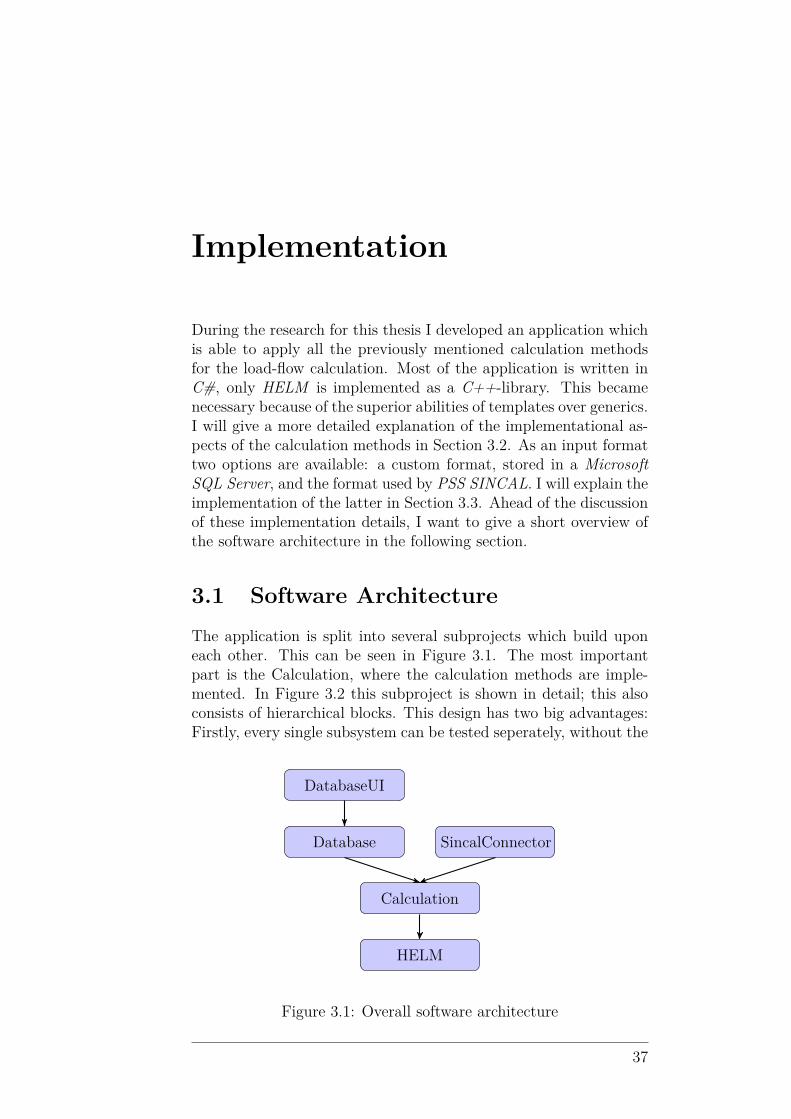
During the research for this thesis I developed an application whichis able to apply all the previously mentioned calculation methodsfor the load-flow calculation. Most of the application is written inC#, only HELM is implemented as a C++-library. This becamenecessary because of the superior abilities of templates over generics.I will give a more detailed explanation of the implementational as-pects of the calculation methods in Section 3.2. As an input formattwo options are available: a custom format, stored in a MicrosoftSQL Server, and the format used by PSS SINCAL. I will explain theimplementation of the latter in Section 3.3. Ahead of the discussionof these implementation details, I want to give a short overview ofthe software architecture in the following section.
3.1 Software ArchitectureThe application is split into several subprojects which build uponeach other. This can be seen in Figure 3.1. The most importantpart is the Calculation, where the calculation methods are imple-mented. In Figure 3.2 this subproject is shown in detail; this alsoconsists of hierarchical blocks. This design has two big advantages:Firstly, every single subsystem can be tested seperately, without the
DatabaseUI
Database SincalConnector
Calculation
HELM
Figure 3.1: Overall software architecture
37

ThreePhase
SinglePhase.MultipleVoltageLevels
SinglePhase.SingleVoltageLevel
Figure 3.2: Software architecture of the subsystem Calculation
necessity to touch the other systems. Secondly, this design is moreflexible. For instance, the consideration of unsymmetric situationscould be achieved through three instances of a single phase net, onefor each symmetric component.
Chapter C shows how the Calculation subsystem can be used.For more complex examples I would like to refer to the code of theunit tests.
3.2 Calculation Methods
3.2.1 Iterative MethodsI implemented all the iterative methods, like the Current Iteration,Newton-Raphson and FDLF, in C#. For the linear algebra I usedthe library math.net numerics1, which has all the necessary toolsimplemented already. This library is obviously not optimized forthis use case. Therefore, it would certainly be possible to speedup the iterative methods, although math.net numerics, for instance,already utilizes multiple cores. As the iterative methods are not themain focus of this work, I focused on HELM and just selected thebest fitting methods from the library, instead of reimplementing andoptimizing them.
3.2.2 Holomorphic Embedding Load FlowFirst of all, I want to explain the design decision to implementHELM as a separate library, written in C++. Unfortunately, insome cases the mantissa of a 64-bit floating point is not sufficientto benefit from the theoretically perfect convergence behaviour ofHELM. The problem here lies within the very small convergenceradius of Equation 2.91. As already mentioned, the theoretical so-lution to this is an analytic continuation, in this case Wynn’s EpsilonAlgorithm. Approximately 50 coefficients already reach the limit ofthe precision of a 64-bit floating point. The calculation of more co-efficients does not improve the results at all because the numerical
38

1 V 1 Ω
P
Figure 3.3: Test net for convergence border
0,2430
0,2440
0,2450
0,2460
0,2470
0,2480
0,2490
0,2500
Current IterationNewton-Raphson
HELM 64-bitwith Current Iteration
P [W
]
HELM 64-bit withNewton-Raphson
HELM 200-bit
HELM 2000-bit
Figure 3.4: Convergence border for Figure 3.3
error, caused by the machine epsilon, is bigger than the possiblegain in accuracy.
To give a more demonstrative explanation, I want to show acomparison between the convergence behaviour of the different al-gorithms. For this purpose I used the net in Figure 3.3, which isstable for P ≤ 0.25 W. In this net I increased the power for aslong as the algorithm converged and noted down the value closestto the border of stability. The result of this procedure is Figure 3.4,in which it can be observed that a more accurate floating pointdatatype enables HELM to get closer to the border of stability.The use of HELM with only 64-bit for the initial voltages already isan improvement over the direct application of the Current Iterationand Newton-Raphson in terms of convergence behaviour. But in theend, only HELM with an arbitrary precise datatype is able to get tothe border of stability as close as desired, although this advantageis traded in for a lot worse performance.
In order to evaluate HELM in detail, even for nets close to theirborder of stability, which can not be calculated with the iterativemethods, I decided to implement HELM with the possibility of aconfigurable precise datatype. As the generics in C# did not giveme the ability to use a library of precise datatypes together witha package for linear algebra, I decided to implement this part inC++. In this language I had templates available, which allowed the
39

combination of MPIR2, a library for multi precision integers andrationals, with a library for sparse linear algebra, like Eigen3.
3.2.3 Linear AlgebraAll the implemented methods have one thing in common: linearalgebra. For all these methods it is necessary to solve linear equationsystems, although the equation systems differ in their properties. InHELM and the Current Iteration method the system matrix is theadmittance matrix, in Newton-Raphson and FDLF it is a Jacobianmatrix. Both types of matrices are typically sparse, therefore the useof sparse linear algebra improves the performance of the algorithmssignificantly.
To solve these linear equation systems with a LU-factorizationis quite slow for big power nets. One possible solution is the use ofiterative solvers like BiCGSTAB [7].
Unfortunately, admittance matrices of power nets are sometimesill-conditioned. Therefore, these iterative solvers may not convergeto an accurate result. In order to be able to handle these powernets, it is necessary to reduce the bandwidth of the admittance ma-trix, for instance through Cuthill-McKee [9]. This method reducesthe overhead caused by fill-ins during the LU-factorization. Conse-quently, the memory usage as well as the total runtime is reducedsignificantly and it is, again, possible to use the LU-factorization fornets with a six digit number of nodes.
The last important detail of the implementation of the calcula-tion methods is the preconditioning. With this step special proper-ties of the system matrix can be leveraged to improve the conditionof the equation system and therefore the iterative solvers are acceler-ated. Fortunately, the admittance matrix, which is the system ma-trix in the Current Iteration and HELM, is approximately diagonaldominant. This makes the application of a diagonal preconditionervery handy because this type of preconditioning is very efficient tocalculate. Furthermore, this preconditioning improves the conditionof the equation system significantly for admittance matrices.
Optimizations
Due to the special circumstances given by HELM a few optimiza-tions are possible, however can not be made in general. At thebeginning I used Eigen for the linear algebra, but with bigger powernets I ran into performance problems with this general purpose li-brary. Consequently, I reimplemented the necessary data structuresand algorithms:
• Dense vector2http://mpir.org/3http://eigen.tuxfamily.org/
40

• Sparse matrix
• Multiplication of a sparse matrix with a dense vector
• Various operations on dense vectors
• BiCGSTAB
• LU-factorization
• Forward and back substitution
The specialization on dense vectors is useful in the case of HELMas the solutions for the equation system are typically dense. There-fore, there is no need to apply more complex operations on sparsevectors.
However, the system matrix of the linear equation system is theadmittance matrix that is sparse for big problems. In fact, theamount of nonzero values in every row is nearly independent of thesize of the total matrix. The reason for this lies within the physicalstructure of a power net, where every node only has a limited numberof neighbours, no matter how big the total graph is. Therefore, thedensity of the admittance matrix decreases with a growing problemsize. For small problems this specialization is, in fact, a performancedrawback, but for these problems the performance does not matterin any case.
As there must not be a zero-row, a version of a sparse matrix withone array for each row is superior to CRS [8] or CCS [8]. Throughthis decision regarding the internal representation of the sparse ma-trix, during the calculation of the LU-decomposition it is possible toavoid a lot of memory reallocations, which become the most expen-sive operations if the sparse matrix is represented internally as CRSor CCS. The decision to store the matrices row- and not column-oriented is related to the matrix multiplication and the forward andbackward substitution, which benefit from this format in terms ofruntime.
The multiplication of a sparse matrix with a dense vector canleverage the special sparse matrix format and the dense vectors.The key point is to only iterate over the nonzero elements at eachrow in the matrix and select the respective elements of the vector inO(1). Additionally, the operation can be parallelized effectively, asall elements in the result vector are independent from each other.
Operations on the dense vectors, like the dot product or addingtwo vectors, can be parallelized as well. With regards to the per-formance of the operations, the dense storage of the values is veryconvenient.
The iterative solver BiCGSTAB benefits from the already op-timized matrix and vector operations. Additionally, it is possibleto avoid a few memory allocations and move operations throughimplementing all these operations in-place.
41

The calculation of a LU-factorization and the forward and back-ward subsitution can not benefit from multiple cores, at least forsmall datatypes like a double, where the floating point operationsare not that expensive. For bigger datatypes with more expensiveoperations there is a small speedup possible.
Additionally, I had to concentrate on numerical stability. Forthis purpose, I sorted all values in ascending order before I summedthem up. This special modification has a negative impact on theperformance, but it improves the convergence behaviour of HELM.
3.3 Link to PSS SINCALThe tool developed during the research for this thesis has a parserfor the file format of PSS SINCAL. This parser allows to read apower net from the file and write back the calculated node voltages.
The basic structure of a power net in PSS SINCAL is as follows:
• ⟨name⟩.sin
• ⟨name⟩ files
– database.001.dia– database.ini– database.mdb
The main information about the electrical characteristics of thepower net are stored in a database, for instance a MS Access database.It is also possible to use Oracle Database or Microsoft SQL Server.However, for this thesis only nets with a MS Access database wereused. Therefore, I only implemented a parser for this configuration.
Fortunately, this database is documented very well online4 andby the documents delivered together with the application.
The most important relations in this database are:
• Terminal: contains information about the connection of thenet elements with the nodes
• VoltageLevel: mostly used for the frequency of the power net
• Element: contains all net elements
• Node: contains all nodes with their ID, name, voltage level,... etc.
• TwoWindingTransformer, ThreeWindingTransformer, Line, Syn-chronousMachine, Load, Infeeder: contain the correspondingnet elements
4http://sincal.s3.amazonaws.com/doc/Misc/SINCAL_Datenbankinterface.pdf; accessed on 14.03.2015
42

• LFNodeResult: contains the node results of the load-flow cal-culation
PSS SINCAL obviously supports a lot more net elements andways to describe them than the tool developed for this thesis sup-ports. Therefore, for more sophisticated or exotic selections in thedatabase the tool will fail to parse the power net. Especially unsym-metric power nets and short circuit calculations are not supportedby this tool. Consequently, the tool neglects the values related tothese calculations.
For more detailed information on the database I would like torefer to the official documentation or the implementation of theparser in the subsystem SincalConnector. This part of the softwarealso has a few unit tests, which may also be used as documentation.
43

44

Results
The most interesting questions regarding HELM are
• How well does HELM perform in comparison to the iterativemethods?
• Is HELM able to calculate large scale power nets, for whichiterative methods do not converge?
To answer these questions I have run several experiments. The onesrelated to the first question can be found in Section 4.1. To answerthe second question I will describe the results of running HELM ona large scale power net with a few thousand nodes in Section 4.2.
4.1 Comparison of the Load-flow Algo-rithms
To compare the different load-flow algorithms I used the sample netsof the Institute and compared the algorithms regarding their run-time and accuracy. I have already considered the improved conver-gence behaviour in Section 3.2.2, but I will show additional resultsregarding this aspect in this chapter.
0,001
0,01
0,1
1
Current Iteration Newton-Raphson HELM 64-bit withCurrent Iteration
σt,rel[1]
Dorfnetz Landnetz Freileitung 1 Landnetz Freileitung 2 Vorstadtnetz Kabel 1 Vorstadtnetz Kabel 2
HELM 64-bit HELM 200-bit
Figure 4.1: Relative standard deviation of the runtime of the algo-rithms
45

0,01
0,1
1
10
100
Current Iteration Newton-Raphson HELM 64-bit withCurrent Iteration
t [s]
Dorfnetz Landnetz Freileitung 1 Landnetz Freileitung 2 Vorstadtnetz Kabel 1 Vorstadtnetz Kabel 2
HELM 64-bit HELM 200-bit
Figure 4.2: Average runtime of the algorithms for several power nets
The selected algorithms for this comparison nearly cover thewhole possible spectrum that is implemented in the tool, includingthe usage of HELM to calculate seed values for an iterative method.This special application of HELM is represented by the algorithmHELM with Current Iteration.
The parameters for the algorithms can be found in Chapter B.The settings for the accuracy and runtime comparison are in Ta-ble B.2, the settings for the convergence border tests are in Ta-ble B.1.
To eliminate influences of other processes or the garbage col-lection at runtime, I ran the calculations five times. The resultingruntimes did not vary much considering the relative standard devi-ations (Figure 4.1).
4.1.1 RuntimeOne key point is the runtime and this not only depends on thealgorithms themselves but also on the used tools like the library forthe sparse linear algebra. Therefore, I am not able to make absolutestatements, especially because I implemented HELM in a differentlanguage than the other algorithms and optimized the linear algebrain HELM.
The first important message here is that HELM with 64-bit isconsiderably fast compared to the Current Iteration and Newton-Raphson, as seen in Figure 4.2. If Newton-Raphson runs into con-vergence problems like in the case of the Vorstadtnetz, HELM iseven faster than this iterative approach.
Another conclusion from these tests is that the combination ofHELM with an iterative method, for instance with the Current It-eration, is very useful. In Section 3.2.2 I have already shown thatthis improves the convergence behaviour, but if we take the runtimeinto account, the combination is not really a drawback. Consideringthis, I recommend to always use HELM with the Current Iterationinstead of only using the latter.
The last important message is the insufficient performance of
46

1E-22
1E-20
1E-18
1E-16
1E-14
1E-12
1E-10
1E-08
1E-06
Current Iteration Newton-Raphson HELM 200-bit withCurrent Iteration
rela
tive
pow
er e
rror
[1]
Dorfnetz Landnetz Freileitung 1 Landnetz Freileitung 2 Vorstadtnetz Kabel 1 Vorstadtnetz Kabel 2
HELM 64-bit HELM 200-bit
Figure 4.3: Relative power error of the algorithms
HELM with a datatype bigger than 64-bit. This setting avoids thatfloating point operations can be executed within a few clock cycleswith the integrated assembler commands and therefore degrades theperformance of the algorithm significantly. Consequently, I recom-mend to use HELM with a bigger datatype only in situations wherethe calculation with HELM with 64-bit failed.
4.1.2 AccuracyAs an accuracy metric I used the relative power error, which isthe ratio between power error and total power, both summed upabsolutely:
εr =∑ |Pi − Pspec,i|+∑ |Qi −Qspec,i|∑ |Pspec,i|+∑ |Qspec,i|
(4.1)
The accuracies of the algorithms (Figure 4.3) were all sufficientfor most applications, although a difference can be seen betweenpure iterative approaches and the ones with HELM. The latter onesare able to deliver more accurate results for these nets.
Keeping in mind that HELM is even as fast as the Current It-eration, there is no reason to use the Current Iteration instead ofHELM. Also, HELM together with the Current Iteration producesmore accurate and reliable results than the Current Iteration only.
47

Figure 4.4: Vorstadtnetz used for the convergence comparison
4.1.3 Convergence
To test and compare the convergence behaviour of the different al-gorithms I used one of the example nets from the Institute, theso-called Vorstadtnetz (Figure 4.4) with nearly 300 nodes. In thisnet I increased the load at the most outer ends of the radial netup to a point, where the algorithm did not converge anymore. Tofind this convergence border more efficiently, I applied the bisectionmethod.
The first and most obvious conclusion, which can be drawn fromFigure 4.5, is that the iterative solver for the internal linear equa-tion systems deteriorates the convergence behaviour of HELM sig-nificantly.
Secondly, at least for this special case, the implementation ofNewton-Raphson in SINCAL has a worse convergence behaviourwith these settings, compared to my implementation. But I wantto make clear that this heavily depends on the settings of the algo-rithm, and I could only guess how certain parameters are actuallyimplemented in SINCAL. Therefore, it is not really possible to drawa meaningful conclusion from this experiment regarding the imple-mention in SINCAL.
If one zooms into this chart one gets Figure 4.6, which revealsthat HELM in its pure form outperforms the other methods, con-sidering the convergence behaviour. After another zoom step onecan see in Figure 4.7 that a more accurate datatype improves theconvergence behaviour of HELM, although only by a few thousandwatts. Additionally, such extrordinary settings affect the runtime ofthe algorithm significantly, as it takes a few hours to calculate thiskind of net, compared to only a few seconds with 64-bit.
48

1,0E+05
1,0E+06
1,0E+07
conv
erge
nce
bord
er [W
]
Figure 4.5: Convergence border of the algorithms
1,80E+06
1,85E+06
1,90E+06
1,95E+06
2,00E+06
conv
erge
nce
bord
er [W
]
Figure 4.6: Convergence border of the algorithms
1,970E+06
1,972E+06
1,974E+06
1,976E+06
HELM, 64-bit, LU HELM, 100-bit, LU HELM, 200-bit, LU HELM, 1000-bit, LU HELM, 10000-bit,LU
conv
erge
nce
bord
er [W
]
Figure 4.7: Convergence border of the algorithms
49

4.2 Calculation of Large-Scale Power NetsTo evaluate HELM in the scenario of large-scale power nets I usedthe power net of infra furth (Figure 4.12), which was kindly providedfor this purpose. Due to the current limitations of HELM, I hadto adapt the power net. For instance, HELM currently does notsupport non-linear current controlled sources, which were used inthe power net of infra furth for the photovoltaic installations, aswell as for the generators. To circumvent this problem I removedall the unsupported elements.
Another important aspect to point out is the switching state.The version I received was configured in a way that the total netwas split up into three parts. For the comparison later on I used thisinitial version, as well as one where the three parts were connectedtogether. In the connected version there was one big net with morethan 50000 nodes.
As algorithms for the comparison I selected:
• HELM with a 64-bit datatype and LU factorization
• Current Iteration with an iterative solver
• HELM with 64-bit datatype and LU factorization and as sec-ond step Current Iteration with an iterative solver
• PSS SINCAL with the default configuration
Unfortunately, the library I used for the linear algebra in the itera-tive load-flow algorithms was not able to calculate the LU factoriza-tion in a reasonable amount of time. Additionally, the calculation ofthe Jacobian matrix was not very efficient either, due to the sparsematrix implementation. Therefore, I had to skip my implementa-tion of FDLF and Newton-Raphson but this class of algorithms isstill represented in the comparison with PSS SINCAL.
As I implemented HELM in C++ and optimized the LU factor-ization for these circumstances, I was able to select this combinationfor the tests. This shows that the performance of the algorithms de-pends heavily on the implementation of the linear algebra.
First, I would like to point out the relative power errors of thealgorithms for these two versions of the power net in Figure 4.8and Figure 4.9. For most applications of a load-flow algorithm thisaccuracy should be sufficient.
Second, the comparison of the runtime in Figure 4.10 and Fig-ure 4.11 shows that HELM is able to get close to the performanceof PSS SINCAL. Contrary, the Current Iteration with the iterativesolver for the linear equation systems is outperformed by HELM andPSS SINCAL by orders of magnitude. Obviously, the main differ-ence is the implementation of the linear algebra, as the admittancematrix is ill-conditioned in these scenarios.
50

1E-10
1E-09
1E-08
1E-07
1E-06HELM (LU) Current Iteration (iterative) HELM (LU) with Current Iteration
rela
tive
pow
er e
rror
[1]
(iterative)
Figure 4.8: relative power error of the algorithms for the separatedversion of the power net of infra furth
1E-12
1E-11
1E-10
1E-09
1E-08
1E-07
1E-06
1E-05
1E-04
1E-03
1E-02
1E-01
1E+00
HELM (LU) Current Iteration (iterative) HELM (LU) with Current Iteration(iterative)
rela
tive
pow
er e
rror
[1]
Figure 4.9: relative power error of the algorithms for the connectedversion of the power net of infra furth
0
200
400
600
800
1000
1200
1400
1600
1800
2000
HELM (LU) Current Iteration(iterative)
HELM (LU) with CurrentIteration (iterative)
PSS SINCAL
elap
sed
time
[s]
Figure 4.10: runtime of the algorithms for the separated version ofthe power net of infra furth
51

0
500
1000
1500
2000
2500
3000
HELM (LU) Current Iteration(iterative)
HELM (LU) with CurrentIteration (iterative)
PSS SINCAL
elap
sed
time
[s]
Figure 4.11: runtime of the algorithms for the connected version ofthe power net of infra furth
Figure 4.12: net of infra furth
52

4.3 ConclusionHELM is superior to the iterative methods with regards to the con-vergence behaviour. This advantage comes directly from the theo-retical background, where so far only for HELM it can be provedto have a perfect convergence behaviour. The only limitation whichis left here is caused by the machine epsilon of the computer. Con-sidering the runtime, HELM can not reach the performance of, forinstance, FDLF if the latter one converges within only a few itera-tions.
In summary, mainly two reasons not to use HELM exist:
1. The calculation has to be done fast
2. A certain control is used in the power net, which is not yetsupported by HELM
The first drawback here is immanent in HELM, but the second onewill be a topic for future research.
Finally, in practical applications it is always handy to have afallback in case the iterative methods do not converge.
53

54

Holomorphic Embedding LoadFlow Example
For the sake of simplicity, only the small net from Figure A.1 iscalculated. This example has no imaginary parts in the solution andthe intermediate results, because only real-valued input parameters(U1 = 1V , Z = 1Ω and P = 0,23W ) are used. The exact solution isdetermined with the current sum on the second node
U1 − U2
Z= P
U2. (A.1)
This is only one quadratic equation
U22 − U1U2 + PZ = 0, (A.2)
whereas the physical solution is
U2 =U1 +
√U2
1 − 4PZ2 (A.3)
=1V +
√(1V )2 − 4 · 0,23W · 1Ω
2 = 0,641421356V. (A.4)
The first 15 coefficients and the tableau of the analytic continu-ation for this example can be found in Table A.1.
As one can see, the result of 0,6414674063V with HELM is al-ready close to the exact solution of 0,641421356V, although only 15coefficients were calculated. This is caused by the very special andminimalistic example. For realistic problems the analytic continua-tion is absolutely necessary to gain reasonable results.
U1Z U2
P
Figure A.1: Power net with two nodes
55

n cn ε(n)0 ε
(n)1 ε
(n)2 ε
(n)3
0 1 1 -4,347826087 0,7012987013 -53,07799786311 -0,23 0,77 -18,9035916824 0,672037037 -123,10562069172 -0,0529 0,7171 -41,094764527 0,6598435294 -228,18340580463 -0,024334 0,692766 -71,4691556991 0,6534624888 -377,22512777194 -0,01399205 0,67877395 -110,9769498434 0,6497065945 -581,38775110125 -0,0090108802 0,6697630698 -160,8361591933 0,647328765 -854,337870536 -0,0062175073 0,6635455625 -222,5006154848 0,6457460789 -1212,63967840137 -0,0044943696 0,6590511929 -297,6596862673 0,6446531589 -1676,23479279968 -0,0033595413 0,6556916516 -388,2517646964 0,6438767511 -2269,01129543989 -0,0025756483 0,6531160033 -496,4856326042 0,6433125844 -3019,468437380710 -0,002014157 0,6511018463 -624,8675009892 0,6428949783 -3961,487835067811 -0,0016003393 0,6495015071 -776,2329204835 0,6425810317 -5135,224910931912 -0,0012882731 0,6482132339 -953,7833616527 0,642341879713 -0,0010484561 0,6471647778 -1161,127570707614 -0,0008612318 0,646303546
n ε(n)4 ε
(n)5 ε
(n)6 ε
(n)7 ε
(n)8
0 0,6577569578 -257,6917202828 0,6463316434 -965,4309176106 0,64293783491 0,65032677 -507,9966791024 0,6441455368 -1793,4498231255 0,64226712522 0,6467529581 -891,5173618297 0,6430368063 -3092,6891389693 0,6419185183 0,6448085383 -1455,9368172673 0,6424258404 -5063,8222472924 0,64172555164 0,6436650919 -2262,8754903897 0,6420688182 -7977,0096092318 0,64161351185 0,6429551357 -3391,1393489018 0,6418507571 -12192,0568935985 0,6415459536 0,6424961042 -4940,6930609089 0,641712852 -18183,7051794566 0,64150393897 0,6421897747 -7037,4691049271 0,6416231356 -26573,19933102898 0,6419800633 -9839,157482384 0,64156337729 0,641833429 -13542,150665957810 0,6417290521
n ε(n)9 ε
(n)10 ε
(n)11 ε
(n)12 ε
(n)13
0 -3284,407797319 0,6418935502 -10759,3888854953 0,6415687586 -34732,50033847561 -5961,2467473499 0,6416851362 -19352,1012790472 0,6415037407 -62254,63259812862 -10246,0728069144 0,6415753189 -33322,845655593 0,64146917673 -16902,4129690484 0,6415144192 -55425,97051998594 -26993,9749727727 0,64147924755 -41985,2383684168
Table A.1: HELM example coefficients and tableau
56

Algorithm Parameters for theComparison
method
targ
etpr
ecisi
on
max
imum
itera
tions
data
type
size
max
imum
coeffi
cien
ts
solv
er
HELM, 64-bit, iterative 1e-10 64 50 iterativeHELM, 64-bit, LU 1e-10 64 50 LUHELM with Current Itera-tion, 64-bit, LU
1e-10 100 64 50 LU
HELM, 100-bit, LU 1e-10 100 70 LUHELM, 200-bit, LU 1e-10 200 100 LUHELM, 1000-bit, LU 1e-10 1000 200 LUHELM, 10000-bit, LU 1e-10 10000 300 LUCurrent Iteration, iterative 1e-10 100 iterativeCurrent Iteration, LU 1e-10 100 LUNewton-Raphson, iterative 1e-10 100 iterativeNewton-Raphson, LU 1e-10 100 LUNewton-Raphson, SINCAL 1e-10 100
Table B.1: Algorithm parameters for the convergence comparison
57

method
targ
etpr
ecisi
on
max
imum
itera
tions
data
type
size
max
imum
coeffi
cien
ts
solv
erCurrent Iteration 1e-5 100 iterativeNewton-Raphson 1e-5 100 iterativeHELM 64-bit 1e-5 64 50 iterativeHELM 200-bit 1e-5 200 100 iterativeHELM 64-bit with CurrentIteration
1e-5 100 64 50 iterative
Table B.2: Algorithm parameters for the runtime and accuracy com-parison
58

Calculation API
var nodeVoltageCalculator = newHolomorphicEmbeddedLoadFlowMethod(1e-5, 50, 64);
var symmetricPowerNet =SymmetricPowerNet.Create(nodeVoltageCalculator, 50);
symmetricPowerNet.AddNode(1, 1000, "source");symmetricPowerNet.AddNode(2, 1000, "load");symmetricPowerNet.AddTransmissionLine(1, 2, 0.0002,
0.0009, 0, 0, 2000, false);symmetricPowerNet.AddFeedIn(1, new Complex(1050, 100),
new Complex());symmetricPowerNet.AddLoad(2, new Complex(-200, -100));
double relativePowerError;var nodeResults =
symmetricPowerNet.CalculateNodeVoltages(outrelativePowerError);
if (nodeResults == null)Console.WriteLine("was not able to calcuate the power
net");else
foreach (var nodeResult in nodeResults)Console.WriteLine("node with ID " + nodeResult.Key
+ " has the voltage " +nodeResult.Value.Voltage + " V");
Console.ReadKey();
59

60

List of Figures
2.1 Sir Adam Beck Hydroelectric Generating Stations . . 122.2 Admittance G between the nodes α and β . . . . . . 142.3 Voltage-controlled current source . . . . . . . . . . . 142.4 Gyrator . . . . . . . . . . . . . . . . . . . . . . . . . 152.5 Equivalent circuit for a gyrator . . . . . . . . . . . . 152.6 Ideal transformer . . . . . . . . . . . . . . . . . . . . 162.7 Equivalent circuit for an ideal transformer . . . . . . 162.8 Equivalent circuit for a transmission line . . . . . . . 182.9 Equivalent circuit for a generator . . . . . . . . . . . 182.10 Equivalent circuit for a transformer . . . . . . . . . . 192.11 Equivalent circuit for a feed-in . . . . . . . . . . . . . 20
3.1 Overall software architecture . . . . . . . . . . . . . . 373.2 Software architecture of the subsystem Calculation . 383.3 Test net for convergence border . . . . . . . . . . . . 393.4 Convergence border for Figure 3.3 . . . . . . . . . . . 39
4.1 Comparison, relative standard deviation of runtime . 454.2 Comparison, average runtime . . . . . . . . . . . . . 464.3 Comparison, accuracy . . . . . . . . . . . . . . . . . 474.4 Vorstadtnetz . . . . . . . . . . . . . . . . . . . . . . . 484.5 Comparison, convergence . . . . . . . . . . . . . . . . 494.6 Comparison, convergence . . . . . . . . . . . . . . . . 494.7 Comparison, convergence . . . . . . . . . . . . . . . . 494.8 Comparison, infra furth, separate, error . . . . . . . . 514.9 Comparison, infra furth, connected, error . . . . . . . 514.10 Comparison, infra furth, separate, runtime . . . . . . 514.11 Comparison, infra furth, connected, runtime . . . . . 524.12 net of infra furth . . . . . . . . . . . . . . . . . . . . 52
A.1 Power net with two nodes . . . . . . . . . . . . . . . 55
61

62

List of Tables
A.1 HELM example coefficients and tableau . . . . . . . . 56
B.1 Algorithm parameters for the convergence comparison 57B.2 Algorithm parameters for the runtime and accuracy
comparison . . . . . . . . . . . . . . . . . . . . . . . 58
63

64

Bibliography
[1] A. Trias, The Holomorphic Embedding Load Flow Method, IEEEPES General Meeting, July 2012
[2] M. K. Subramanian, Y. Feng, D. Tylavsky, PV Bus Modelingin a Holomorphically Embedded Power-Flow Formulation, 978-1-4799-1255-1/13, IEEE, 2013
[3] A. Trias, System and Method for Monitoring and ManagingElectrical Power Transmission and Distribution Networks, USPatent 7,519,506 B2, April 2009
[4] A. Trias, System and Method for Monitoring and ManagingElectrical Power Transmission and Distribution Networks, USPatent US 2009/0228154 A1, September 2009
[5] P. Wynn, The Epsilon Algorithm and Operational Formulas ofNumerical Analysis, June 1960
[6] H. Saadat, Power System Analysis, ISBN 0-07-012235-0,McGraw-Hill, 1999
[7] H. A. van der Vorst, Bi-CGSTAB: A Fast and Smoothly Con-verging Variant of Bi-CG for the Solution of Nonsymmetric Lin-ear Systems, ISSN 2168-3417, SIAM Journal on Scientific andStatistical Computing, Volume 13, 1992
[8] M. Lujan, A. Usman, P. Hardie, T. L. Freeman, J. R. Gurd,Storage Formats for Sparse Matrices in Java, ComputationalScience – ICCS 2005: 5th International Conference, Proceedings,Springer Science & Business Media, 2005
[9] E. Cuthill, J. McKee, Reducing the Bandwidth of Sparse Sym-metric Matrices, Naval Ship Research and Development Center,Washington DC
[10] B. Stott, O. Alsac, Fast Decoupled Load Flow, ISSN 0018-9510,Power Apparatus and Systems, IEEE Transactions on (Volume:PAS-93, Issue: 3), May 1974
65