implementation and optimisation techniquesgweddell/cs848/dlhb-09.pdf · ian horrocks abstract ......

9

Implementation and Optimisation TechniquesIan Horrocks

Abstract

This chapter will discuss the implementation of the reasoning services which formthe core of Description Logic based Knowledge Representation Systems. To beuseful in realistic applications, such systems need both expressive logics and fastreasoners. As expressive logics inevitably have high worst-case complexities, thiscan only be achieved by employing highly optimised implementations of suitablereasoning algorithms. Systems based on such implementations have demonstratedthat they can perform well with problems that occur in realistic applications, in-cluding problems where unoptimised reasoning is hopelessly intractable.

9.1 Introduction

The usefulness of Description Logics (DLs) in applications has been hindered by thebasic conflict between expressiveness and tractability. Realistic applications typi-cally require both expressive logics, with inevitably high worst case complexities fortheir decision procedures, and acceptable performance from the reasoning services.Although the definition of acceptable may vary widely from application to appli-cation, early experiments with DLs indicated that, in practice, performance was aserious problem, even for logics with relatively limited expressive powers [Heinsohnet al., 1992].

On the other hand, theoretical work has continued to extend our understandingof the boundaries of decidability in DLs, and has led to the development of soundand complete reasoning algorithms for much more expressive logics. The expressivepower of these logics goes a long way towards addressing the criticisms levelled atDLs in traditional applications such as ontological engineering [Doyle and Patil,1991] and is sufficient to suggest that they could be useful in several exciting newapplication domains, for example reasoning about DataBase schemata and queries[Calvanese et al., 1998f; 1998a] and providing reasoning support for the so-called

313

314 I. Horrocks

Semantic Web [Decker et al., 2000; Bechhofer et al., 2001b]. However, the worstcase complexity of their decision procedures is invariably (at least) exponential withrespect to problem size.

This high worst case complexity initially led to the conjecture that expressiveDLs might be of limited practical applicability [Buchheit et al., 1993c]. However,although the theoretical complexity results are discouraging, empirical analysesof real applications have shown that the kinds of construct which lead to worstcase intractability rarely occur in practice [Nebel, 1990b; Heinsohn et al., 1994;Speel et al., 1995], and experiments with the Kris system showed that apply-ing some simple optimisation techniques could lead to a significant improvementin the empirical performance of a DL system [Baader et al., 1992a]. More re-cently the Fact, Dlp and Racer systems have demonstrated that, even withvery expressive logics, highly optimised implementations can provide accept-able performance in realistic applications [Horrocks and Patel-Schneider, 1999;Haarslev and Moller, 2001c].1

In this chapter we will study the implementation of DL systems, examining indetail the wide range of optimisation techniques that can be used to improve perfor-mance. Some of the techniques that will be discussed are completely independentof the logical language supported by the DL and the kind of algorithm used forreasoning; many others would be applicable to a wide range of languages and im-plementation styles, particularly those using search based algorithms. However, thedetailed descriptions of implementation and optimisation techniques will assume,for the most part, reasoning in an expressive DL based on a sound and completetableaux algorithm.

9.1.1 Performance analysis

Before designing and implementing a DL based Knowledge Representation System,the implementor should be clear about the goals that they are trying to meet andagainst which the performance of the system will ultimately be measured. In thischapter it will be assumed that the primary goal is utility in realistic applications,and that this will normally be assessed by empirical analysis.

Unfortunately, as DL systems with very expressive logics have only recently be-come available [Horrocks, 1998a; Patel-Schneider, 1998; Haarslev and Moller, 2001e],there are very few applications that can be used as a source for test data.2 Oneapplication that has been able to provide such data is the European Galen project,part of which has involved the construction of a large DL Knowledge Base describing

1 It should be pointed out that experience in this area is still relatively limited.2 This situation is changing rapidly, however, with the increasing use of DLs in DataBase and ontology

applications.

Implementation and Optimisation Techniques 315

medical terminology [Rector et al., 1993]. Reasoning performance with respect tothis knowledge base has been used for comparing DL systems [Horrocks and Patel-Schneider, 1998b], and we will often refer to it when assessing the effectiveness ofoptimisation techniques.

As few other suitable knowledge bases are available, the testing of DL systemshas often been supplemented with the use of randomly generated or hand craftedtest data [Giunchiglia and Sebastiani, 1996b; Heuerding and Schwendimann, 1996;Horrocks and Patel-Schneider, 1998b; Massacci, 1999; Donini and Massacci, 2000].In many cases the data was originally developed for testing propositional modallogics, and has been adapted for use with DLs by taking advantage of the well knowcorrespondence between the two formalisms [Schild, 1991]. Tests using this kindof data, in particular the test suites from the Tableaux’98 comparison of modallogic theorem provers [Balsiger and Heuerding, 1998] and the DL’98 comparisonof DL systems [Horrocks and Patel-Schneider, 1998b], will also be referred to inassessments of optimisation techniques.

9.2 Preliminaries

This section will introduce the syntax and semantics of DLs (full details of whichcan be found in Chapter 2) and discuss the reasoning services which would formthe core of a Description Logic based Knowledge Representation System. It willalso discuss how, through the use of unfolding and internalisation, these reasoningservices can often be reduced to the problem of determining the satisfiability of asingle concept.

9.2.1 Syntax and semantics

DLs are formalisms that support the logical description of concepts and roles. Ar-bitrary concept and role descriptions (from now on referred to simply as conceptsand roles) are constructed from atomic concept and role names using a variety ofconcept and role forming operators, the range of which is dependent on the par-ticular logic. In the following discussion we will use C and D to denote arbitraryconcepts, R and S to denote arbitrary roles, A and P to denote atomic concept androle names, and n to denote a nonnegative integer.

For concepts, the available operators usually include some or all of the standardlogical connectives, conjunction (denoted u), disjunction (denoted t) and negation(denoted ¬). In addition, the universal concept top (denoted >, and equivalent toAt¬A) and the incoherent concept bottom (denoted⊥, and equivalent to Au¬A) areoften predefined. Other commonly supported operators include restricted forms ofquantification called existential role restrictions (denoted ∃R.C) and universal role

316 I. Horrocks

restrictions (denoted ∀R.C). Some DLs also support qualified number restrictions(denoted 6n .PC and >n .PC), operators that place cardinality restrictions on theroles relating instances of a concept to instances of some other concept. Cardinalityrestrictions are often limited to the forms 6n .P> and > n .P>, when they arecalled unqualified number restrictions, or simply number restrictions, and are oftenabbreviated to 6 nP and > nP. The roles that can appear in cardinality restrictionconcepts are usually restricted to being atomic, as allowing arbitrary roles in suchconcepts is known no lead to undecidability [Baader and Sattler, 1996b].

Role forming operators may also be supported, and in some very expressive logicsroles can be regular expressions formed using union (denoted t), composition (de-noted ◦), reflexive-transitive closure (denoted ∗) and identity operators (denoted id),possibly augmented with the inverse (also known as converse) operator (denoted −)[De Giacomo and Lenzerini, 1996]. In most implemented systems, however, rolesare restricted to being atomic names.

Concepts and roles are given a standard Tarski style model theoretic semantics,their meaning being given by an interpretation I = (∆I ,I ), where ∆I is the domain(a set) and I is an interpretation function. Full details of both syntax and semanticscan be found in Chapter 2.

In general, a DL knowledge base (KB) consists of a set T of terminological axioms,and a set A of assertional axioms. The axioms in T state facts about concepts androles while those in A state facts about individual instances of concepts and roles.As in this chapter we will mostly be concerned with terminological reasoning, thatis reasoning about concepts and roles, a KB will usually be taken to consist only ofthe terminological component T .

A terminological KB T usually consists of a set of axioms of the form C v D andC ≡ D, where C and D are concepts. An interpretation I satisfies T if for everyaxiom (C v D) ∈ T , CI ⊆ DI , and for every axiom (C ≡ D) ∈ T , CI = DI ; T issatisfiable if there exists some non empty interpretation that satisfies it. Note thatT can, without loss of generality, be restricted to contain only inclusion axioms oronly equality axioms, as the two forms can be reduced one to the other using thefollowing equivalences:

C v D ⇐⇒ > ≡ D t ¬C

C ≡ D ⇐⇒ C v D and D v C

A concept C is subsumed by a concept D with respect to T (written T |= C v D)if CI ⊆ DI in every interpretation I that satisfies T , a concept C is satisfiable withrespect to T (written T |= C 6v ⊥) if CI 6= ∅ in some I that satisfies T , and aconcept C is unsatisfiable (not satisfiable) with respect to T (written T |= ¬C) ifCI = ∅ in every I that satisfies T . Subsumption and (un)satisfiability are closely


related. If T |= C v D, then in all interpretations I that satisfy T , CI ⊆ DI andso CI ∩ (¬D)I = ∅. Conversely, if C is not satisfiable with respect to T , then in allI that satisfy T , CI = ∅ and so CI ⊆ ⊥I . Subsumption and (un)satisfiability canthus be reduced one to the other using the following equivalences:

T |= C v D ⇐⇒ T |= ¬(C u ¬D)

T |= ¬C ⇐⇒ T |= C v ⊥

In some DLs T can also contain axioms that define a set of transitive roles R+

and/or a subsumption partial ordering on roles [Horrocks and Sattler, 1999]. Anaxiom R ∈ R+ states that R is a transitive role while an axiom R v S states thatR is subsumed by S. An interpretation I satisfies the axiom R ∈ R+ if RI istransitively closed (i.e, (RI)+ = RI), and it satisfies the axiom R v S if RI ⊆ SI .

9.2.2 Reasoning services

Terminological reasoning in a DL based Knowledge Representation System is basedon determining subsumption relationships with respect to the axioms in a KB. Aswell as answering specific subsumption and satisfiability queries, it is often useful tocompute and store (usually in the form of a directed acyclic graph) the subsumptionpartial ordering of all the concept names appearing in the KB, a procedure knownas classifying the KB [Patel-Schneider and Swartout, 1993]. Some systems mayalso be capable of dealing with assertional axioms, those concerning instances ofconcepts and roles, and performing reasoning tasks such as realisation (determiningthe concepts instantiated by a given individual) and retrieval (determining the setof individuals that instantiate a given concept) [Baader et al., 1991]. However,we will mostly concentrate on terminological reasoning as it has been more widelyused in DL applications. Moreover, given a sufficiently expressive DL, assertionalreasoning can be reduced to terminological reasoning [De Giacomo and Lenzerini,1996].

In practice, many systems use subsumption testing algorithms that are not ca-pable of determining subsumption relationships with respect to an arbitrary KB.Instead, they restrict the kinds of axiom that can appear in the KB so that de-pendency eliminating substitutions (known as unfolding) can be performed prior toevaluating subsumption relationships. These restrictions require that all axioms areunique, acyclic definitions. An axiom is called a definition of A if it is of the formA v D or A ≡ D, where A is an atomic name, it is unique if the KB contains noother definition of A, and it is acyclic if D does not refer either directly or indirectly(via other axioms) to A. A KB that satisfies these restrictions will be called anunfoldable KB.

Definitions of the form A v D are sometimes called primitive or necessary, as

318 I. Horrocks

D specifies a necessary condition for instances of A, while those of the form A ≡D are sometimes called non-primitive or necessary and sufficient as D specifiesconditions that are both necessary and sufficient for instances of A. In order todistinguish non-definitional axioms, they are often called general axioms [Buchheitet al., 1993a]. Restricting the KB to definition axioms makes reasoning much easier,but significantly reduces the expressive power of the DL. However, even with anunrestricted (or general) KB, definition axioms and unfolding are still useful ideas,as they can be used to optimise the reasoning procedures (see Section 9.4.3).

9.2.3 Unfolding

Given an unfoldable KB T , and a concept C whose satisfiability is to be testedwith respect to T , it is possible to eliminate from C all concept names occurringin T using a recursive substitution procedure called unfolding. The satisfiability ofthe resulting concept is independent of the axioms in T and can therefore be testedusing a decision procedure that is only capable of determining the satisfiability ofa single concept (or equivalently, the satisfiability of a concept with respect to anempty KB).

For a non-primitive concept name A, defined in T by an axiom A ≡ D, theprocedure is simply to substitute A with D wherever it occurs in C, and then torecursively unfold D. For a primitive concept name A, defined in T by an axiomA v D, the procedure is slightly more complex. Wherever A occurs in C it issubstituted with the concept A′ uD, where A′ is a new concept name not occurringin T or C, and D is then recursively unfolded. The concept A′ represents the“primitiveness” of A—the unspecified characteristics that differentiate it from D.We will use Unfold(C, T ) to denote the concept C unfolded with respect to a KBT .

A decision procedure that tries to find a satisfying interpretation I for the un-folded concept can now be used, as any such interpretation will also satisfy T . Thiscan easily be shown by applying the unfolding procedure to all of the concepts form-ing the right hand side of axioms in T , so that they are constructed entirely fromconcept names that are not defined in T , and are thus independent of the otheraxioms in T . The interpretation of each defined concept in T can then be taken tobe the interpretation of the unfolded right hand side concept, as given by I and thesemantics of the concept and role forming operators.

Subsumption reasoning can be made independent of T using the same technique.Given two concepts C and D, determining if C is subsumed by D with respect toT is the same as determining if Unfold(C, T ) is subsumed by Unfold(D, T ) with


respect to an empty KB:

T |= C v D ⇐⇒ ∅ |= Unfold(C, T ) v Unfold(D, T )

Unfolding would not be possible, in general, if the axioms in T were not uniqueacyclic definitions. If T contained multiple definition axioms for some concept A,for example {(A ≡ C), (A ≡ D)} ⊆ T , then it would not be possible to makea substitution for A that preserved the meaning of both axioms. If T containedcyclical axioms, for example (A v ∃R.A) ∈ T , then trying to unfold A would leadto non-termination. If T contained general axioms, for example ∃R.C v D, thenit could not be guaranteed that an interpretation satisfying the unfolded conceptwould also satisfy these axioms.

9.2.4 Internalisation

While it is possible to design an algorithm capable of reasoning with respect to ageneral KB [Buchheit et al., 1993a], with more expressive logics, in particular thoseallowing the definition of a universal role, a procedure called internalisation canbe used to reduce the problem to that of determining the satisfiability of a singleconcept [Baader, 1991]. A truly universal role is one whose interpretation includesevery pair of elements in the domain of interpretation (i.e., ∆I ×∆I). However, arole U is universal w.r.t. a terminology T if it is defined such that U is transitivelyclosed and P v U for all role names P occurring in T . For a logic that supports theunion and transitive reflexive closure role forming operators, this can be achievedsimply by taking U to be

(P1 t . . . t Pn t P−1 t . . . t P−n )∗,

where P1, . . . , Pn are all the roles names occurring in T . For a logic that supportstransitively closed roles and role inclusion axioms, this can be achieved by addingthe axioms

(U ∈ R+), (P1 v U), . . . , (Pn v U), (P−1 v U), . . . , (P−n v U)

to T , where P1, . . . , Pn are all the roles names occurring in T and U is a new rolename not occurring in T . Note that in either case, the inverse role components areonly required if the logic supports the inverse role operator.

The concept axioms in T can be reduced to axioms of the form > v C using theequivalences:

A ≡ B ⇐⇒ > v (A t ¬B) u (¬A tB)

A v B ⇐⇒ > v ¬A tB

320 I. Horrocks

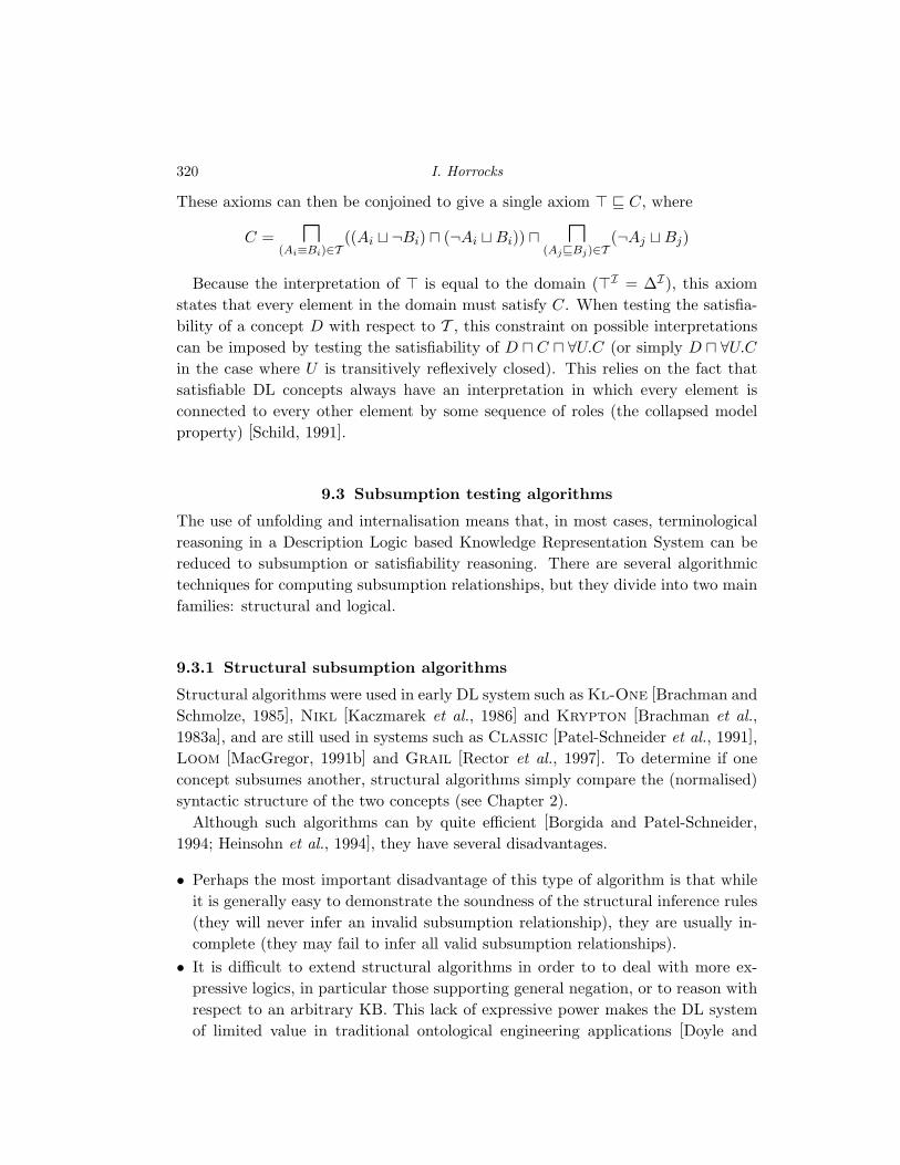
These axioms can then be conjoined to give a single axiom > v C, where

C = u(Ai≡Bi)∈T

((Ai t ¬Bi) u (¬Ai tBi)) u u(AjvBj)∈T

(¬Aj tBj)

Because the interpretation of > is equal to the domain (>I = ∆I), this axiomstates that every element in the domain must satisfy C. When testing the satisfia-bility of a concept D with respect to T , this constraint on possible interpretationscan be imposed by testing the satisfiability of D u C u ∀U.C (or simply D u ∀U.Cin the case where U is transitively reflexively closed). This relies on the fact thatsatisfiable DL concepts always have an interpretation in which every element isconnected to every other element by some sequence of roles (the collapsed modelproperty) [Schild, 1991].

9.3 Subsumption testing algorithms

The use of unfolding and internalisation means that, in most cases, terminologicalreasoning in a Description Logic based Knowledge Representation System can bereduced to subsumption or satisfiability reasoning. There are several algorithmictechniques for computing subsumption relationships, but they divide into two mainfamilies: structural and logical.

9.3.1 Structural subsumption algorithms

Structural algorithms were used in early DL system such as Kl-One [Brachman andSchmolze, 1985], Nikl [Kaczmarek et al., 1986] and Krypton [Brachman et al.,1983a], and are still used in systems such as Classic [Patel-Schneider et al., 1991],Loom [MacGregor, 1991b] and Grail [Rector et al., 1997]. To determine if oneconcept subsumes another, structural algorithms simply compare the (normalised)syntactic structure of the two concepts (see Chapter 2).

Although such algorithms can by quite efficient [Borgida and Patel-Schneider,1994; Heinsohn et al., 1994], they have several disadvantages.

• Perhaps the most important disadvantage of this type of algorithm is that whileit is generally easy to demonstrate the soundness of the structural inference rules(they will never infer an invalid subsumption relationship), they are usually in-complete (they may fail to infer all valid subsumption relationships).

• It is difficult to extend structural algorithms in order to to deal with more ex-pressive logics, in particular those supporting general negation, or to reason withrespect to an arbitrary KB. This lack of expressive power makes the DL systemof limited value in traditional ontological engineering applications [Doyle and


Patil, 1991], and completely useless in DataBase schema reasoning applications[Calvanese et al., 1998f].

• Although accepting some degree of incompleteness is one way of improving theperformance of a DL reasoner, the performance of incomplete reasoners is highlydependent on the degree of incompleteness, and this is notoriously difficult toquantify [Borgida, 1992a].

9.3.2 Logical algorithms

These kinds of algorithm use a refutation style proof: C is subsumed by D if itcan be shown that the existence of an individual x that is in the extension of C(x ∈ CI) but not in the extension of D (x /∈ DI) is logically inconsistent. As wehave seen in Section 9.2.2, this corresponds to testing the logical (un)satisfiabilityof the concept C u¬D (i.e., C v D iff C u¬D is not satisfiable). Note that formingthis concept obviously relies on having full negation in the logic.

Various techniques can be used to test the logical satisfiability of a concept.One obvious possibility is to exploit an existing reasoner. For example, the Log-icsWorkbench [Balsiger et al., 1996], a general purpouse proposition modal logicreasoning system, could be used simply by exploiting the well known correspon-dences between description and modal logics [Schild, 1991]. First order logic the-orem provers can also be used via appropriate traslations of DLs into first or-der logic. Examples of this approach can be seen in systems developed by Hus-tadt and Schmidt [1997], using the Spass theorem prover, and Paramasivam andPlaisted [1998], using the CLIN-S theorem prover. An existing reasoner could alsobe used as a component of a more powerful system, as in Ksat/*Sat [Giunchigliaand Sebastiani, 1996a; Giunchiglia et al., 2001a], where a propositional satisfiability(SAT) tester is used as the key component of a propositional modal satisfiabilityreasoner.

There are advantages and disadvantages to the “re-use” approach. On the positiveside, it should be much easier to build a system based on an existing reasoner, andperformance can be maximised by using a state of the art implementation suchas Spass (a highly optimised first order theorem prover) or the highly optimisedSAT testing algorithms used in Ksat and *Sat (the use of a specialised SAT testerallows *Sat to outperform other systems on classes of problem that emphasisepropositional reasoning). The translation (into first order logic) approach has alsobeen shown to be able to deal with a wide range of expressive DLs, in particularthose with complex role forming operators such as negation or identity [Hustadtand Schmidt, 2000].

On the negative side, it may be difficult to extend the reasoner to deal with moreexpressive logics, or to add optimisations that take advantage of specific features

322 I. Horrocks

of the DL, without reimplementing the reasoner (as has been done, for example, inmore recent versions of the *Sat system).

Most, if not all, implemented DL systems based on logical reasoning have usedcustom designed tableaux decision procedures. These algorithms try to prove thatD subsumes C by starting with a single individual satisfying C u ¬D, and demon-strating that any attempt to extend this into a complete interpretation (using a setof tableaux expansion rules) will lead to a logical contradiction. If a complete andnon-contradictory interpretation is found, then this represents a counter example(an interpretation in which some element of the domain is in CI but not in DI)that disproves the conjectured subsumption relationship.

This approach has many advantages and has dominated recent DL research:

• it has a sound theoretical basis in first order logic [Hollunder et al., 1990];• it can be relatively easily adapted to allow for a range of logical languages by

changing the set of tableaux expansion rules [Hollunder et al., 1990; Bresciani etal., 1995];

• it can be adapted to deal with very expressive logics, and to reason with respectto an arbitrary KB, by using more sophisticated control mechanisms to ensuretermination [Baader, 1991; Buchheit et al., 1993c; Sattler, 1996];

• it has been shown to be optimal for a number of DL languages, in the sense thatthe worst case complexity of the algorithm is no worse than the known complexityof the satisfiability problem for the logic [Hollunder et al., 1990].

In the remainder of this chapter, detailed descriptions of implementation andoptimisation techniques will assume the use of a tableaux decision procedure. How-ever, many of the techniques are independent of the subsumption testing algorithmor could easily be adapted to most logic based methods. The reverse is also true,and several of the described techniques have been adapted from other logical de-cision procedures, in particular those that try to optimise the search used to dealwith non-determinism.

9.3.2.1 Tableaux algorithms

Tableaux algorithms try to prove the satisfiability of a concept D by constructinga model, an interpretation I in which DI is not empty. A tableau is a graph whichrepresents such a model, with nodes corresponding to individuals (elements of ∆I)and edges corresponding to relationships between individuals (elements of ∆I×∆I).

A typical algorithm will start with a single individual satisfying D and try toconstruct a tableau, or some structure from which a tableau can be constructed,by inferring the existence of additional individuals or of additional constraints onindividuals. The inference mechanism consists of applying a set of expansion rules


which correspond to the logical constructs of the language, and the algorithm ter-minates either when the structure is complete (no further inferences are possible)or obvious contradictions have been revealed. Non-determinism is dealt with bysearching different possible expansions: the concept is unsatisfiable if every expan-sion leads to a contradiction and is satisfiable if any possible expansion leads to thediscovery of a complete non-contradictory structure.

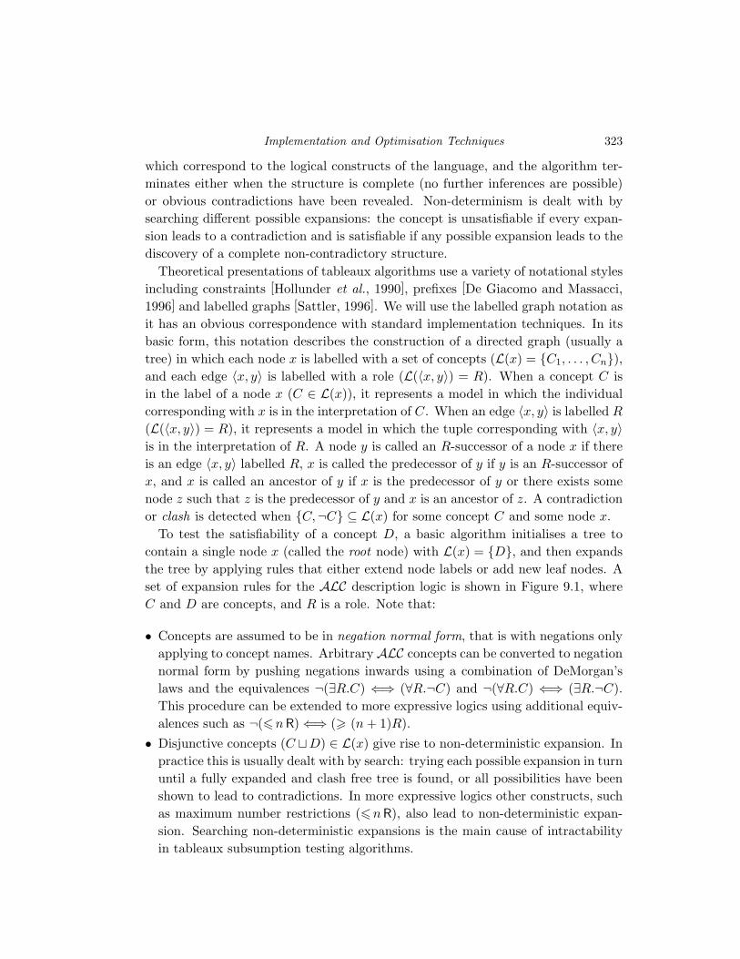
Theoretical presentations of tableaux algorithms use a variety of notational stylesincluding constraints [Hollunder et al., 1990], prefixes [De Giacomo and Massacci,1996] and labelled graphs [Sattler, 1996]. We will use the labelled graph notation asit has an obvious correspondence with standard implementation techniques. In itsbasic form, this notation describes the construction of a directed graph (usually atree) in which each node x is labelled with a set of concepts (L(x) = {C1, . . . , Cn}),and each edge 〈x, y〉 is labelled with a role (L(〈x, y〉) = R). When a concept C isin the label of a node x (C ∈ L(x)), it represents a model in which the individualcorresponding with x is in the interpretation of C. When an edge 〈x, y〉 is labelled R(L(〈x, y〉) = R), it represents a model in which the tuple corresponding with 〈x, y〉is in the interpretation of R. A node y is called an R-successor of a node x if thereis an edge 〈x, y〉 labelled R, x is called the predecessor of y if y is an R-successor ofx, and x is called an ancestor of y if x is the predecessor of y or there exists somenode z such that z is the predecessor of y and x is an ancestor of z. A contradictionor clash is detected when {C,¬C} ⊆ L(x) for some concept C and some node x.

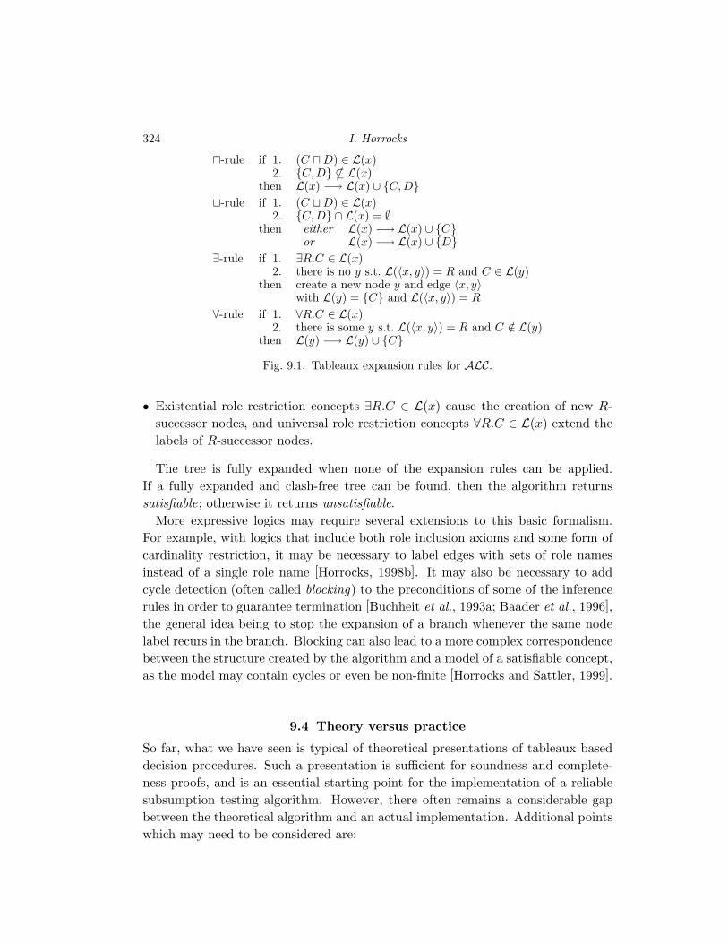
To test the satisfiability of a concept D, a basic algorithm initialises a tree tocontain a single node x (called the root node) with L(x) = {D}, and then expandsthe tree by applying rules that either extend node labels or add new leaf nodes. Aset of expansion rules for the ALC description logic is shown in Figure 9.1, whereC and D are concepts, and R is a role. Note that:

• Concepts are assumed to be in negation normal form, that is with negations onlyapplying to concept names. Arbitrary ALC concepts can be converted to negationnormal form by pushing negations inwards using a combination of DeMorgan’slaws and the equivalences ¬(∃R.C) ⇐⇒ (∀R.¬C) and ¬(∀R.C) ⇐⇒ (∃R.¬C).This procedure can be extended to more expressive logics using additional equiv-alences such as ¬(6n R) ⇐⇒ (> (n + 1)R).

• Disjunctive concepts (C tD) ∈ L(x) give rise to non-deterministic expansion. Inpractice this is usually dealt with by search: trying each possible expansion in turnuntil a fully expanded and clash free tree is found, or all possibilities have beenshown to lead to contradictions. In more expressive logics other constructs, suchas maximum number restrictions (6nR), also lead to non-deterministic expan-sion. Searching non-deterministic expansions is the main cause of intractabilityin tableaux subsumption testing algorithms.

324 I. Horrocks

u-rule if 1. (C uD) ∈ L(x)2. {C,D} * L(x)

then L(x) −→ L(x) ∪ {C, D}t-rule if 1. (C tD) ∈ L(x)

2. {C, D} ∩ L(x) = ∅then either L(x) −→ L(x) ∪ {C}

or L(x) −→ L(x) ∪ {D}∃-rule if 1. ∃R.C ∈ L(x)

2. there is no y s.t. L(〈x, y〉) = R and C ∈ L(y)then create a new node y and edge 〈x, y〉

with L(y) = {C} and L(〈x, y〉) = R∀-rule if 1. ∀R.C ∈ L(x)

2. there is some y s.t. L(〈x, y〉) = R and C /∈ L(y)then L(y) −→ L(y) ∪ {C}

Fig. 9.1. Tableaux expansion rules for ALC.

• Existential role restriction concepts ∃R.C ∈ L(x) cause the creation of new R-successor nodes, and universal role restriction concepts ∀R.C ∈ L(x) extend thelabels of R-successor nodes.

The tree is fully expanded when none of the expansion rules can be applied.If a fully expanded and clash-free tree can be found, then the algorithm returnssatisfiable; otherwise it returns unsatisfiable.

More expressive logics may require several extensions to this basic formalism.For example, with logics that include both role inclusion axioms and some form ofcardinality restriction, it may be necessary to label edges with sets of role namesinstead of a single role name [Horrocks, 1998b]. It may also be necessary to addcycle detection (often called blocking) to the preconditions of some of the inferencerules in order to guarantee termination [Buchheit et al., 1993a; Baader et al., 1996],the general idea being to stop the expansion of a branch whenever the same nodelabel recurs in the branch. Blocking can also lead to a more complex correspondencebetween the structure created by the algorithm and a model of a satisfiable concept,as the model may contain cycles or even be non-finite [Horrocks and Sattler, 1999].

9.4 Theory versus practice

So far, what we have seen is typical of theoretical presentations of tableaux baseddecision procedures. Such a presentation is sufficient for soundness and complete-ness proofs, and is an essential starting point for the implementation of a reliablesubsumption testing algorithm. However, there often remains a considerable gapbetween the theoretical algorithm and an actual implementation. Additional pointswhich may need to be considered are:


• the efficiency of the algorithm, in the theoretical (worst case) sense;• the efficiency of the algorithm, in a practical (typical case) sense;• how to use the algorithm for reasoning with unfoldable, general and cyclical KBs;• optimising the (implementation of the) algorithm to improve the typical case

performance.

In the remainder of this Section we will consider the first three points, while inthe following section we will consider implementation and optimisation techniquesin detail.

9.4.1 Worst case complexity

When considering an implementation, it is sensible to start with an algorithm that isknown to be theoretically efficient, even if the implementation subsequently departsfrom the theory to some extent. Theoretically efficient is taken to mean that thecomplexity of the algorithm is equal to the complexity of the satisfiability problemfor the logic, where this is known, or at least that consideration has been givento the worst case complexity of the algorithm. This is not always the case, asthe algorithm may have been designed to facilitate a soundness and completenessproof, with little consideration having been given to worst case complexity, muchless implementation.

Apart from establishing an upper bound for the “hardness” of the problem, stud-ies of theoretical complexity can suggest useful implementation techniques. Forexample, a study of the complexity of the satisfiability problem for ALC conceptswith respect to a general KB has demonstrated that caching of intermediate resultsis required in order to stay in ExpTime [Donini et al., 1996a], while studying thecomplexity of the satisfiability problem for SIN concepts has shown that a moresophisticated labelling and blocking strategy can be used in order to stay in PSpace[Horrocks et al., 1999].

One theoretically derived technique that is widely used in practice is the tracetechnique. This is a method for minimising the amount of space used by the algo-rithm to store the tableaux expansion tree. The idea is to impose an ordering onthe application of expansion rules so that local propositional reasoning (finding aclash-free expansion of conjunctions and disjunctions using the u-rule and t-rule)is completed before new nodes are created using the ∃-rule. A successor created byan application of the ∃-rule, and any possible applications of the ∀-rule, can thenbe treated as an independent sub-problem that returns either satisfiable or unsatis-fiable, and the space used to solve it can be reused in solving the next sub-problem.A node x returns satisfiable if there is a clash-free propositional solution for whichany and all sub-problems return satisfiable; otherwise it returns unsatisfiable. In

326 I. Horrocks

∃∀-rule if 1. ∃R.C ∈ L(x)2. there is no y s.t. L(〈x, y〉) = R and C ∈ L(y)3. neither the u-rule nor the t-rule is applicable to L(x)

then create a new node y and edge 〈x, y〉with L(y) = {C} ∪ {D | ∀R.D ∈ L(x)} and L(〈x, y〉) = R

Fig. 9.2. Combined ∃∀-rule for ALC.

algorithms where the trace technique can be used, the ∀-rule is often incorporatedin the ∃-rule, giving a single rule as shown in Figure 9.2.

Apart from minimising space usage the trace technique is generally viewed as asensible way of organising the expansion and the flow of control within the algorithm.Ordering the expansion in this way may also be required by some blocking strategies[Buchheit et al., 1993a], although in some cases it is possible to use a more efficientsubset blocking technique that is independent of the ordering [Baader et al., 1996].

The trace technique relies on the fact that node labels are not affected by theexpansion of their successors. This is no longer true when the logic includes inverseroles, because universal value restrictions in the label of a successor of a node x canaugment L(x). This could invalidate the existing propositional solution for L(x), orinvalidate previously computed solutions to sub-problems in other successor nodes.For example, if

L(x) = {∃R.C, ∃S.(∀S−.(∀R.¬C))},

then x is obviously unsatisfiable as expanding ∃S.(∀S−.(∀R.¬C)) will add ∀R.¬Cto L(x), meaning that x must have an R-successor whose label contains both Cand ¬C. The contradiction would not be discovered if the R-successor required by∃R.C ∈ L(x) were generated first, found to be satisfiable and then deleted from thetree in order to save space.

The development of a PSpace algorithm for the SIN logic has shown that amodified version of the trace technique can still be used with logics that includeinverse roles [Horrocks et al., 1999]. However, the modification requires that thepropositional solution and all sub-problems are re-computed whenever the label ofa node is augmented by the expansion of a universal value restriction in the labelof one of its successors.

9.4.2 Typical case complexity

Although useful practical techniques can be derived from the study of theoreticalalgorithms, it should be borne in mind that minimising worst case complexity mayrequire the use of techniques that clearly would not be sensible in typical cases.This is because the kinds of pathological problem that would lead to worst case


behaviour do not seem to occur in realistic applications. In particular, the amountof space used by algorithms does not seem to be a practical problem, whereas thetime taken for the computation certainly is. For example, in experiments withthe Fact system using the DL’98 test suite, available memory (200Mb) was neverexhausted in spite of the fact that some single computations required hundreds ofseconds of CPU time [Horrocks and Patel-Schneider, 1998b]. In other experimentsusing the Galen KB, computations were run for tens of thousands of seconds ofCPU time without exhausting available memory.

In view of these considerations, techniques that save space by recomputing areunlikely to be of practical value. The modified trace technique used in the PSpaceSIN algorithm (see Section 9.4.1), for example, is probably not of practical value.However, the more sophisticated labelling and blocking strategy, which allows theestablishment a polynomial bound on the length of branches, could be used notonly in an implementation of the SIN algorithm, but also in implementations ofmore expressive logics where other considerations mean that the PSpace result nolonger holds [Horrocks et al., 1999].

In practice, the poor performance of tableaux algorithms is due to non-determinism in the expansion rules (for example the t-rule), and the resultingsearch of different possible expansions. This is often treated in a very cursory man-ner in theoretical presentations. For soundness and completeness it is enough toprove that the search will always find a solution if one exists, and that it will alwaysterminate. For worst case complexity, an upper bound on the size of the search spaceis all that is required. As this upper bound is invariably exponential with respect tothe size of the problem, exploring the whole search space would inevitably lead tointractability for all but the smallest problems. When implementing an algorithmit is therefore vital to give much more careful consideration to non-deterministicexpansion, in particular how to reduce the size of the search space and how to ex-plore it in an efficient manner. Many of the optimisations discussed in subsequentsections will be aimed at doing this, for example by using absorption to localisenon-determinism in the KB, dependency directed backtracking to prune the searchtree, heuristics to guide the search, and caching to avoid repetitive search.

9.4.3 Reasoning with a knowledge base

One area in which the theory and practice diverge significantly is that of reasoningwith respect to the axioms in a KB. This problem is rarely considered in detail:with less expressive logics the KB is usually restricted to being unfoldable, whilewith more expressive logics, all axioms can be treated as general axioms and dealtwith via internalisation. In either case it is sufficient to consider an algorithm thattests the satisfiability of a single concept, usually in negation normal form.

328 I. Horrocks

In practice, it is much more efficient to retain the structure of the KB for as longas possible, and to take advantage of it during subsumption/satisfiability testing.One way in which this can be done is to use lazy unfolding—only unfolding conceptsas required by the progress of the subsumption or satisfiability testing algorithm[Baader et al., 1992a]. With a tableaux algorithm, this means that a defined conceptA is only unfolded when it occurs in a node label. For example, if T containsthe non-primitive definition axiom A ≡ C, and the u-rule is applied to a concept(A u D) ∈ L(x) so that A and D are added to L(x), then at this point A can beunfolded by substituting it with C.

Used in this way, lazy unfolding already has the advantage that it avoids unnec-essary unfolding of irrelevant sub-concepts, either because a contradiction is dis-covered without fully expanding the tree, or because a non-deterministic expansionchoice leads to a complete and clash free tree. However, a much greater increase inefficiency can be achieved if, instead of substituting concept names with their def-initions, names are retained when their definitions are added. This is because thediscovery of a clash between concept names can avoid expansion of their definitions[Baader et al., 1992a].

In general, lazy unfolding can be described as additional tableaux expansion rules,defined as follows.

U1-rule if 1. A ∈ L(x) and (A ≡ C) ∈ T2. C /∈ L(x)

then L(x) −→ L(x) ∪ {C}U2-rule if 1. ¬A ∈ L(x) and (A ≡ C) ∈ T

2. ¬C /∈ L(x)then L(x) −→ L(x) ∪ {¬C}

U3-rule if 1. A ∈ L(x) and (A v C) ∈ T2. C /∈ L(x)

then L(x) −→ L(x) ∪ {C}

The U1-rule and U2-rule reflect the symmetry of the equality relation in the non-primitive definition A ≡ C, which is equivalent to A v C and ¬A v ¬C. TheU3-rule on the other hand reflects the asymmetry of the subsumption relation inthe primitive definition A v C.

Treating all the axioms in the KB as general axioms, and dealing with themvia internalisation, is also highly inefficient. For example, if T contains an axiomA v C, where A is a concept name not appearing on the left hand side of any otheraxiom, then it is easy to deal with the axiom using the lazy unfolding technique,simply adding C to the label of any node in which A appears. Treating all axioms


as general axioms would be equivalent to applying the following additional tableauxexpansion rules:

I1-rule if 1. (C ≡ D) ∈ T2. (D t ¬C) /∈ L(x)

then L(x) −→ L(x) ∪ {(D t ¬C)}I2-rule if 1. (C ≡ D) ∈ T

2. (¬D t C) /∈ L(x)then L(x) −→ L(x) ∪ {(¬D t C)}

I3-rule if 1. (C v D) ∈ T2. (D t ¬C) /∈ L(x)

then L(x) −→ L(x) ∪ {(D t ¬C)}

With (A v C) ∈ T , this would result in the disjunction (Ct¬A) being added to thelabel of every node, leading to non-deterministic expansion and search, the maincause of empirical intractability.

The solution to this problem is to divide the KB into two components, an un-foldable part Tu and a general part Tg, such that Tg = T \ Tu, and Tu containsunique, acyclical, definition axioms. This is easily achieved, e.g., by initialising Tu

to ∅ (which is obviously unfoldable), then for each axiom X in T , adding X to Tu

if Tu ∪X is still unfoldable, and adding X to Tg otherwise.1 It is then possible touse lazy unfolding to deal with Tu, and internalisation to deal with Tg.

Given that the satisfiability testing algorithm includes some sort of cycle checking,such as blocking, then it is even possible to be a little less conservative with respectto the definition of Tu by allowing it to contain cyclical primitive definition axioms,for example axioms of the form A v ∃R.A. Lazy unfolding will ensure that AI ⊆∃R.AI by adding ∃R.A to every node containing A, while blocking will take care ofthe non-termination problem that such an axiom would otherwise cause [Horrocks,1997b]. Moreover, multiple primitive definitions for a single name can be added toTu, or equivalently merged into a single definition using the equivalence

(A v C1), . . . , (A v Cn) ⇐⇒ A v (C1 u . . . u Cn)

However, if Tu contains a non-primitive definition axiom A ≡ C, then it cannotcontain any other definitions for A, because this would be equivalent to allowinggeneral axioms in Tu. For example, given a general axiom C v D, this could beadded to Tu as A v D and A ≡ C, where A is a new name not appearing in T .Moreover, certain kinds of non-primitive cycles cannot be allowed as they can beused to constrain possible models a way that would not be reflected by unfolding.For example, if (A ≡ ¬A) ∈ T for some concept name A, then the domain of all1 Note that the result may depend on the order in which the axioms in T are processed.

330 I. Horrocks

valid interpretations of T must be empty, and T |= C v D for all concepts C andD [Horrocks and Tobies, 2000].

9.5 Optimisation techniques

The Kris system demonstrated that by taking a well designed tableaux algorithm,and applying some reasonable implementation and optimisation techniques (such aslazy expansion), it is possible to obtain a tableaux based DL system that behavesreasonably well in typical cases, and compares favourably with systems based onstructural algorithms [Baader et al., 1992a]. However, this kind of system is stillmuch too slow to be usable in many realistic applications. Fortunately, it is possibleto achieve dramatic improvements in typical case performance by using a widerrange of optimisation techniques.

As DL systems are often used to classify a KB, a hierarchy of optimisation tech-niques is naturally suggested based on the stage of the classification process at whichthey can be applied.

(i) Preprocessing optimisations that try to modify the KB so that classificationand subsumption testing are easier.

(ii) Partial ordering optimisations that try to minimise the number of subsump-tion tests required in order to classify the KB

(iii) Subsumption optimisations that try to avoid performing a potentially expen-sive satisfiability test, usually by substituting a cheaper test.

(iv) Satisfiability optimisations that try to improve the typical case performanceof the underlying satisfiability tester.

9.5.1 Preprocessing optimisations

The axioms that constitute a DL KB may have been generated by a human knowl-edge engineer, as is typically the case in ontological engineering applications, or bethe result of some automated mapping from another formalism, as is typically thecase in DB schema and query reasoning applications. In either case it is unlikelythat a great deal of consideration was given to facilitating the subsequent reasoningprocedures; the KB may, for example, contain considerable redundancy and maymake unnecessary use of general axioms. As we have seen, general axioms are costlyto reason with due to the high degree of non-determinism that they introduce.

It is, therefore, useful to preprocess the KB, applying a range of syntactic simpli-fications and manipulations. The first of these, normalisation, tries to simplify theKB by identifying syntactic equivalences, contradictions and tautologies. The sec-ond, absorption, tries to eliminate general axioms by augmenting definition axioms.


9.5.1.1 Normalisation

In realistic KBs, at least those manually constructed, large and complex concepts areseldom described monolithically, but are built up from a hierarchy of named conceptswhose descriptions are less complex. The lazy unfolding technique described abovecan use this structure to provide more rapid detection of contradictions.

The effectiveness of lazy unfolding is greatly increased if a contradiction betweentwo concepts can be detected whenever one is syntactically equivalent to the nega-tion of the other; for example, we would like to discover a direct contradictionbetween (C u D) and (¬D t ¬C). This can be achieved by transforming all con-cepts into a syntactic normal form, and by directly detecting contradictions causedby non-atomic concepts as well as those caused by concept names.

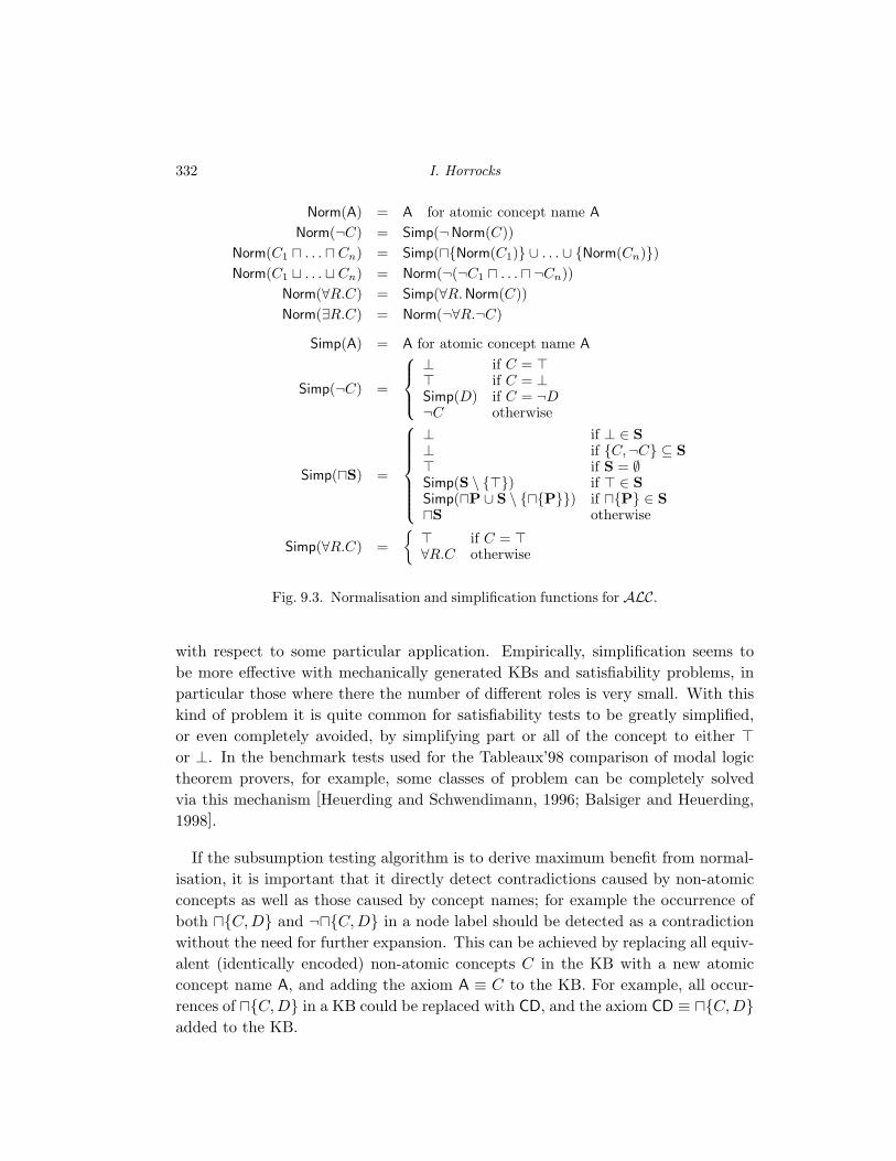
In DLs there is often redundancy in the set of concept forming operators. Inparticular, logics with full negation often provide pairs of operators, either one ofwhich can be eliminated in favour of the other by using negation. Conjunction anddisjunction operators are an example of such a pair, and one can be eliminated infavour of the other using DeMorgan’s laws. In syntactic normal form, all conceptsare transformed so that only one of each such pair appears in the KB (it does notmatter which of the two is chosen, the important thing is uniformity). In ALC, forexample, all concepts could be transformed into (possibly negated) value restric-tions, conjunctions and atomic concept names, with (¬D t ¬C) being transformedinto ¬(D u C). An important refinement is to treat conjunctions as sets (writtenu{C1, . . . , Cn}) so that reordering or repeating the conjuncts does not effect equiv-alence; for example, (D uC) would be normalised as u{C, D}.1 Normalisation canalso include a range of simplifications so that syntactically obvious contradictionsand tautologies are detected; for example, ∃R.⊥ could be simplified to ⊥.

Figure 9.3 describes normalisation and simplification functions Norm and Simpfor ALC. These can be extended to deal with more expressive logics by addingappropriate normalisations (and possibly additional simplifications). For example,number restrictions can be dealt with by adding the normalisations Norm(6 nR) =¬> (n + 1)R and Norm(> nR) = > nR, and the simplification Simp(> 0R) = >.

Normalised and simplified concepts may not be in negation normal form, but theycan be dealt with by treating them exactly like their non-negated counterparts. Forexample, ¬u{C, D} can be treated as (¬C t ¬D) and ¬∀R.C can be treated as∃R.¬C. In the remainder of this chapter we will use both forms interchangeably,choosing whichever is most convenient.

Additional simplifications would clearly be possible. For example, ∀R.C u ∀R.Dcould be simplified to ∀R. Norm(C u D). Which simplifications it is sensible toperform is an implementation decision that may depend on a cost-benefit analysis

1 Sorting the elements in conjuctions, and eliminating duplicates, achieves the same result.

332 I. Horrocks

Norm(A) = A for atomic concept name ANorm(¬C) = Simp(¬Norm(C))

Norm(C1 u . . . u Cn) = Simp(u{Norm(C1)} ∪ . . . ∪ {Norm(Cn)})Norm(C1 t . . . t Cn) = Norm(¬(¬C1 u . . . u ¬Cn))

Norm(∀R.C) = Simp(∀R. Norm(C))Norm(∃R.C) = Norm(¬∀R.¬C)

Simp(A) = A for atomic concept name A

Simp(¬C) =

⊥ if C = >> if C = ⊥Simp(D) if C = ¬D¬C otherwise

Simp(uS) =

⊥ if ⊥ ∈ S⊥ if {C,¬C} ⊆ S> if S = ∅Simp(S \ {>}) if > ∈ SSimp(uP ∪ S \ {u{P}}) if u{P} ∈ SuS otherwise

Simp(∀R.C) ={

> if C = >∀R.C otherwise

Fig. 9.3. Normalisation and simplification functions for ALC.

with respect to some particular application. Empirically, simplification seems tobe more effective with mechanically generated KBs and satisfiability problems, inparticular those where there the number of different roles is very small. With thiskind of problem it is quite common for satisfiability tests to be greatly simplified,or even completely avoided, by simplifying part or all of the concept to either >or ⊥. In the benchmark tests used for the Tableaux’98 comparison of modal logictheorem provers, for example, some classes of problem can be completely solvedvia this mechanism [Heuerding and Schwendimann, 1996; Balsiger and Heuerding,1998].

If the subsumption testing algorithm is to derive maximum benefit from normal-isation, it is important that it directly detect contradictions caused by non-atomicconcepts as well as those caused by concept names; for example the occurrence ofboth u{C, D} and ¬u{C, D} in a node label should be detected as a contradictionwithout the need for further expansion. This can be achieved by replacing all equiv-alent (identically encoded) non-atomic concepts C in the KB with a new atomicconcept name A, and adding the axiom A ≡ C to the KB. For example, all occur-rences of u{C,D} in a KB could be replaced with CD, and the axiom CD ≡ u{C,D}added to the KB.


It is necessary to distinguish these newly introduced system names from usernames appearing in the original KB, as system names need not be classified (indeed,it would be very confusing for the user if they were). In practice, it is often moreconvenient to avoid this problem by using pointer or object identifiers to refer toconcepts, with the same identifier always being associated with equivalent concepts.A contradiction is then detected whenever a pointer/identifier and its negation occurin a node label.

The advantages of the normalisation and simplification procedure are:

• It is easy to implement and could be used with most logics and algorithms.• Subsumption/satisfiability problems can often be simplified, and sometimes even

completely avoided, by detecting syntactically obvious satisfiability and unsatis-fiability.

• It complements lazy unfolding and improves early clash detection.• The elimination of redundancies and the sharing of syntactically equivalent struc-

tures may lead to the KB being more compactly stored.

The disadvantages are:

• The overhead involved in the procedure, although this is relatively small.• For very unstructured KBs there may be no benefit, and it might even slightly

increase size of KB.

9.5.1.2 Absorption

As we have seen in Section 9.4.3, general axioms are costly to reason with due to thehigh degree of non-determinism that they introduce. With a tableaux algorithm,a disjunction is added to the label of each node for each general axiom in the KB.This leads to an exponential increase in the search space as the number of nodesand axioms increases. For example, with 10 nodes and a KB containing 10 generalaxioms there are already 100 disjunctions, and they can be non-deterministicallyexpanded in 2100 different ways. For a KB containing large numbers of generalaxioms (there are 1,214 in the Galen medical terminology KB) this can degradeperformance to the extent that subsumption testing is effectively non-terminating.

It therefore makes sense to eliminate general axioms from the KB whenever possi-ble. Absorption is a technique that tries to do this by absorbing them into primitivedefinition axioms. The basic idea is that a general axiom of the form C v D, whereC may be a non-atomic concept, is manipulated (using the equivalences in Fig-ure 9.4) so that it has the form of a primitive definition A v D′, where A is anatomic concept name. This axiom can then be merged into an existing primitivedefinition A v C ′ to give A v C ′ uD′. For example, an axiom stating that all three

334 I. Horrocks

C1 u C2 v D ⇐⇒ C1 v D t ¬C2

C v D1 uD2 ⇐⇒ C v D1 and C v D2

Fig. 9.4. Axiom equivalences used in absorption.

sided geometric figures (i.e., triangles) also have three angles

geometric-figure u ∃angles.three v ∃sides.three

could be transformed into an axiom stating that all geometric figures either havethree sides or do not have three angles

geometric-figure v ∃sides.three t ¬∃angles.three

and then absorbed into the primitive definition of geometric figure(geometric-figure v figure) to give

geometric-figure v figure u (∃sides.three t ¬∃angles.three).

Given a KB divided into an unfoldable part Tu and a general part Tg, the followingprocedure can be used to try to absorb the axioms from Tg into primitive definitionsin Tu. First a set T ′g is initialised to be empty, and any axioms (C ≡ D) ∈ Tg arereplaced with an equivalent pair of axioms C v D and ¬C v ¬D. Then for eachaxiom (C v D) ∈ Tg:

(i) Initialise a set G = {¬D,C}, representing the axiom in the form > v¬u{¬D, C} (i.e. > v D t ¬C).

(ii) If for some A ∈ G there is a primitive definition axiom (A v C) ∈ Tu,then absorb the general axiom into the primitive definition axiom so that itbecomes

A v u{C,¬u(G \ {A})},

and exit.(iii) If for some A ∈ G there is an axiom (A ≡ D) ∈ Tu, then substitute A ∈ G

with D

G −→ {D} ∪G \ {A},

and return to step (ii).(iv) If for some ¬A ∈ G there is an axiom (A ≡ D) ∈ Tu, then substitute ¬A ∈ G

with ¬D

G −→ {¬D} ∪G \ {¬A},

and return to step (ii).


(v) If there is some C ∈ G such that C is of the form uS, then use associativityto simplify G

G −→ S ∪G \ {uS},

and return to step (ii).(vi) If there is some C ∈ G such that C is of the form ¬uS, then for every D ∈ S

try to absorb (recursively)

{¬D} ∪G \ {¬uS},

and exit.(vii) Otherwise, the axiom could not be absorbed, so add ¬uG to T ′g

T ′g −→ T ′g ∪ ¬uG,

and exit.

Note that this procedure allows parts of axioms to be absorbed. For example, givenaxioms (A v D1) ∈ Tu and (A t ∃R.C v D2) ∈ Tg, then the general axiom wouldbe partly absorbed into the definition axiom to give (A v (D1 uD2)) ∈ Tu, leavinga smaller general axiom (¬u{¬D2,∃R.C}) ∈ Tg.

When this procedure has been applied to all the axioms in Tg, then T ′g representsthose (parts of) axioms that could not be absorbed. The axioms in T ′g are alreadyin the form > v C, so that uT ′g is the concept that must be added to every nodein the tableaux expansion. This can be done using a universal role, as describe inSection 9.2.4, although in practice it may be simpler just to add the concept to thelabel of each newly created node.

The absorption process is clearly non-deterministic. In the first place, there maybe more than one way to divide T into unfoldable and general parts. For example, ifT contains multiple non-primitive definitions for some concept A, then one of themmust be selected as a definition in Tu while the rest are treated as general axioms inTg. Moreover, the absorption procedure itself is non-deterministic as G may containmore than one primitive concept name into which the axiom could be absorbed. Forexample, in the case where {A1, A2} = G, and there are two primitive definitionaxioms A1 v C and A2 v D in Tu, then the axiom could be absorbed either intothe definition of A1 to give A1 v C u ¬u{A2} (equivalent to A1 v C u ¬A2) or intothe definition of A2 to give A2 v C u ¬u{A1} (equivalent to A2 v C u ¬A1).

It would obviously be sensible to choose the “best” absorption (the one that max-imised empirical tractability), but it is not clear how to do this—in fact it is not evenclear how to define “best” in this context [Horrocks and Tobies, 2000]. If T containsmore than one definition axiom for a given concept name, then empirical evidencesuggests that efficiency is improved by retaining as many non-primitive definition

336 I. Horrocks

axioms in Tu as possible. Another intuitively obvious possibility is to preferentiallyabsorb into the definition axiom of the most specific primitive concept, althoughthis only helps in the case that A1 v A2 or A2 v A1. Other more sophisticatedschemes might be possible, but have yet to be investigated.

The advantages of absorption are:

• It can lead to a dramatic improvement in performance. For example, withoutabsorption, satisfiability of the Galen KB (i.e., the satisfiability of >) could notbe proved by either Fact or Dlp, even after several weeks of CPU time. Afterabsorption, the problem becomes so trivial that the CPU time required is hardto measure.

• It is logic and algorithm independent.

The disadvantage is the overhead required for the pre-processing, although this isgenerally small compared to classification times. However, the procedure describedis almost certainly sub-optimal, and trying to find an optimal absorption may bemuch more costly.

9.5.2 Optimising classification

DL systems are often used to classify a KB, that is to compute a partial orderingor hierarchy of named concepts in the KB based on the subsumption relationship.As subsumption testing is always potentially costly, it is important to ensure thatthe classification process uses the smallest possible number of tests. Minimising thenumber of subsumption tests required to classify a concept in the concept hierarchycan be treated as an abstract order-theoretic problem which is independent of theordering relation. However, some additional optimisation can be achieved by usingthe structure of concepts to reveal obvious subsumption relationships and to controlthe order in which concepts are added to the hierarchy (where this is possible).

The concept hierarchy is usually represented by a directed acyclic graph wherenodes are labelled with sets of concept names (because multiple concept namesmay be logically equivalent), and edges correspond with subsumption relationships.The subsumption relation is both transitive and reflexive, so a classified concept Asubsumes a classified concept B if either:

(i) both A and B are in the label of some node x, or(ii) A is in the label of some node x, there is an edge 〈x, y〉 in the graph, and the

concept(s) in the label of node y subsume B.

It will be assumed that the hierarchy always contains a top node (a node whoselabel includes >) and a bottom node (a node whose label includes ⊥) such that the


top node subsumes the bottom node. If the KB is unsatisfiable then the hierarchywill consist of a single node whose label includes both > and ⊥.

Algorithms based on traversal of the concept hierarchy can be used to minimisethe number of tests required in order to add a new concept [Baader et al., 1992a].The idea is to compute a concept’s subsumers by searching down the hierarchy fromthe top node (the top search phase) and its subsumees by searching up the hierarchyfrom the bottom node (the bottom search phase).

When classifying a concept A, the top search takes advantage of the transitivityof the subsumption relation by propagating failed results down the hierarchy. Itconcludes, without performing a subsumption test, that if A is not subsumed by B,then it cannot be subsumed by any other concept that is subsumed by B:

T 6|= A v B and T |= B′ v B implies T 6|= A v B′

To maximise the effect of this strategy, a modified breadth first search is used [Ellis,1992] which ensures that a test to discover if B subsumes A is never performed untilit has been established that A is subsumed by all of the concepts known to subsumeB.

The bottom search uses a corresponding technique, testing if A subsumes B onlywhen A is already known to subsume all those concepts that are subsumed by B.Information from the top search is also used by confining the bottom search to thoseconcepts which are subsumed by all of A’s subsumers.

This abstract partial ordering technique can be enhanced by taking advantage ofthe structure of concepts and the axioms in the KB. If the KB contains an axiomA v C or A ≡ C, then C is said to be a told subsumer of A. If C is a conjunctiveconcept (C1 u . . . u Cn), then from the structural subsumption relationship

D v (C1 u · · · u Cn) implies D v C1 and · · · and D v Cn

it is possible to conclude that C1, . . . , Cn are also told subsumers of A. Moreover, dueto the transitivity of the subsumption relation, any told subsumers of C1, . . . , Cn arealso told subsumers of A. Before classifying A, all of its told subsumers which havealready been classified, and all their subsumers, can be marked as subsumers of A;subsumption tests with respect to these concepts are therefore rendered unnecessary.This idea can be extended in the obvious way to take advantage of a structuralsubsumption relationship with respect to disjunctive concepts,

(C1 t · · · t Cn) v D implies C1 v D and · · · and Cn v D.

If the KB contains an axiom A ≡ C and C is a disjunctive concept (C1 t . . . tCn),then A is a told subsumer of C1, . . . , Cn.

To maximise the effect of the told subsumer optimisation, concepts should beclassified in definition order. This means that a concept A is not classified until all

338 I. Horrocks

of its told subsumers have been classified. When classifying an unfoldable KB, thisordering can be exploited by omitting the bottom search phase for primitive con-cept names and assuming that they only subsume (concepts equivalent to) ⊥. Thisis possible because, with an unfoldable KB, a primitive concept can only subsumeconcepts for which it is a told subsumer. Therefore, as concepts are classified indefinition order, a primitive concept will always be classified before any of the con-cepts that it subsumes. This additional optimisation cannot be used with a generalKB because, in the presence of general axioms, it can no longer be guaranteed thata primitive concept will only subsume concepts for which it is a told subsumer. Forexample, given a KB T such that

T = {A v ∃R.C, ∃R.C v B},

then B is not a told subsumer of A, and A may be classified first. However, whenB is classified the bottom search phase will discover that it subsumes A due to theaxiom ∃R.C v B.

The advantages of the enhanced traversal classification method are:

• It can significantly reduce the number of subsumption tests required in order toclassify a KB [Baader et al., 1992a].

• It is logic and (subsumption) algorithm independent.

There appear to be few disadvantages to this method, and it is used (in someform) in most implemented DL systems.

9.5.3 Optimising subsumption testing

The classification optimisations described in Section 9.5.2 help to reduce the num-ber of subsumption tests that are performed when classifying a KB, and the com-bination of normalisation, simplification and lazy unfolding facilitates the detectionof “obvious” subsumption relationships by allowing unsatisfiability to be rapidlydemonstrated. However, detecting “obvious” non-subsumption (satisfiability) ismore difficult for tableaux algorithms. This is unfortunate as concept hierarchiesfrom realistic applications are typically broad, shallow and tree-like. The top searchphase of classifying a new concept A in such a hierarchy will therefore result in sev-eral subsumption tests being performed at each node, most of which are likely tofail. These failed tests could be very costly (if, for example, proving the satisfiabilityof A is a hard problem), and they could also be very repetitive.

This problem can be tackled by trying to use cached results from previoustableaux tests to prove non-subsumption without performing a new satisfiability


R1

{C1} {C2}

R1

{C1} {C2}

R2

{C3}

{C3}

R3

R3R2

{A, C, ∃R1.C1, ∃R2.C2} {¬B, D, ∃R3.C3}

{A,¬B, C, D,∃R1.C1, ∃R2.C2, ∃R3.C3}

Fig. 9.5. Joining expansion trees for A and ¬B.

test. For example, given two concepts A and B defined by the axioms

A ≡ C u ∃R1.C1 u ∃R2.C2, and

B ≡ ¬D t ∀R3.¬C3,

then A is not subsumed by B if the concept A u ¬B is satisfiable. If tableauxexpansion trees for A and ¬B have already been cached, then the satisfiability ofthe conjunction can be demonstrated by a tree consisting of the trees for A and ¬Bjoined at their root nodes, as shown in Figure 9.5 (note that ¬B ≡ D u ∃R3.C3).

Given two fully expanded and clash free tableaux expansion trees T1 and T2

representing models of (satisfiable) concepts A and ¬B respectively, the tree createdby joining T1 and T2 at their root nodes is a fully expanded and clash free treerepresenting a model of Au¬B provided that the union of the root node labels doesnot contain a clash and that no tableaux expansion rules are applicable to the newtree. For most logics, this can be ascertained by examining the labels of the rootnodes and the labels of the edges connection them with their successors. With theALC logic for example, if x1 and x2 are the two root nodes, then the new tree willbe fully expanded and clash free provided that

(i) the union of the root node labels does not contain an immediate contradic-tion, i.e., there is no C such that {C,¬C} ⊆ L(x1) ∪ L(x2), and

(ii) there is no interaction between value restrictions in the label of one root nodeand edges connecting the other root node with its successors that might makethe ∀-rule applicable to the joined tree, i.e., there is no R such that ∀R.C ∈L(x1) and T2 has an edge 〈x2, y〉 with L(〈x2, y〉) = R, or ∀R.C ∈ L(x2) andT1 has an edge 〈x1, y〉 with L(〈x1, y〉) = R.

340 I. Horrocks

With more expressive logics it may be necessary to consider other interactions thatcould lead to the application of tableaux expansion rules. With a logic that includednumber restrictions, for example, it would be necessary to check that these couldnot be violated by the root node successors in the joined tree.

It would be possible to join trees in a wider range of cases by examining thepotential interactions in more detail. For example, a value restriction ∀R.C ∈ L(x1)and an R labelled edge 〈x2, y〉 would not make the ∀-rule applicable to the joined treeif C ∈ L(x2). However, considering only root nodes and edges provides a relativelyfast test and reduces the storage required by the cache. Both the time requiredby the test and the size of the cache can be reduced even further by only storingrelevant components of the root node labels and edges from the fully expanded andclash free tree that demonstrates the satisfiability of a concept. In the case of ALC,the relevant components from a tree demonstrating the satisfiability of a conceptA are the set of (possibly negated) atomic concept names in the root node label(denoted Lc(A)), the set of role names in value restrictions in the root node label(denoted L∀(A)), and the set of role names labelling edges connecting the root nodewith its successors (denoted L∃(A)).1 These components can be cached as a triple(Lc(A),L∀(A),L∃(A)).

When testing if A is subsumed by B, the algorithm can now proceed as follows.

(i) If any of (Lc(A),L∀(A),L∃(A)), (Lc(¬A),L∀(¬A),L∃(¬A)), (Lc(B),L∀(B),L∃(B)) or (Lc(¬B),L∀(¬B),L∃(¬B)) are not in the cache, then perform theappropriate satisfiability tests and update the cache accordingly. In the casewhere a concept C is unsatisfiable, Lc(C) = {⊥} and Lc(¬C) = {>}.

(ii) Conclude that A v B (A u ¬B is not satisfiable) if Lc(A) = {⊥} or Lc(B) ={>}.

(iii) Conclude that A 6v B (A u ¬B is satisfiable) if

(a) Lc(A) = {>} and Lc(B) 6= {>}, or(b) Lc(A) 6= {⊥} and Lc(B) = {⊥}, or(c) L∀(A)uL∃(B) = ∅, L∀(B)uL∃(A) = ∅, ⊥ /∈ Lc(A)∪Lc(B), and there

is no C such that {C,¬C} ⊆ Lc(A) ∪ Lc(B).

(iv) Otherwise perform a satisfiability test on A u ¬B, concluding that A v B ifit is not satisfiable and that A 6v B if it is satisfiable.

When a concept A is added to the hierarchy, this procedure will result in satisfia-bility tests immediately being performed for both A and ¬A. During the subsequenttop search phase, at each node x in the hierarchy such that some C ∈ L(x) sub-sumes A, it will be necessary to perform a subsumption test for each subsumee1 Consideration can be limited to atomic concept names because expanded conjunction and disjunction

concepts are no longer relevant to the validity of the tree, and are only retained in order to facilitateearly clash detection.


node y (unless some of them can be avoided by the classification optimisations dis-cussed in Section 9.5.2). Typically only one of these subsumption tests will lead toa full satisfiability test being performed, the rest being shown to be obvious non-subsumptions using the cached partial trees. Moreover, the satisfiability test that isperformed will often be an “obvious” subsumption, and unsatisfiability will rapidlybe demonstrated.

The optimisation is less useful during the bottom search phase as nodes in theconcept hierarchy are typically connected to only one subsuming node. The ex-ception to this is the bottom (⊥) node, which may be connected to a very largenumber of subsuming nodes. Again, most of the subsumption tests that would berequired by these nodes can be avoided by demonstrating non-subsumption usingcached partial trees.

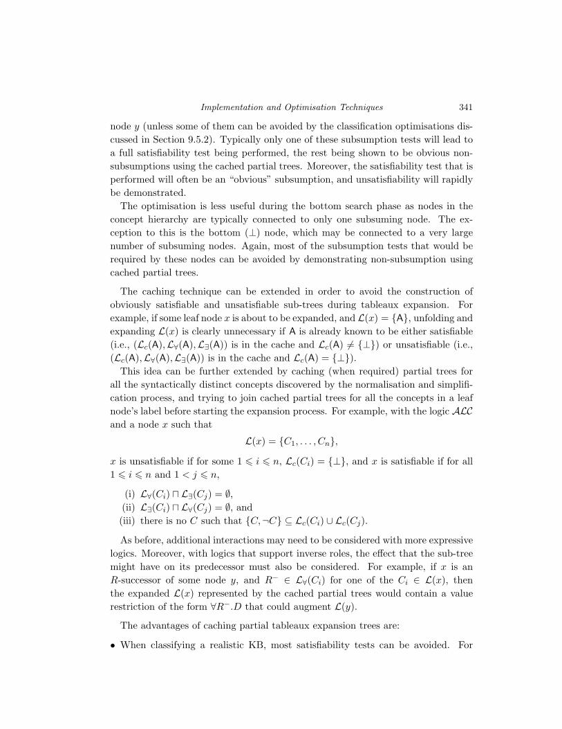
The caching technique can be extended in order to avoid the construction ofobviously satisfiable and unsatisfiable sub-trees during tableaux expansion. Forexample, if some leaf node x is about to be expanded, and L(x) = {A}, unfolding andexpanding L(x) is clearly unnecessary if A is already known to be either satisfiable(i.e., (Lc(A),L∀(A),L∃(A)) is in the cache and Lc(A) 6= {⊥}) or unsatisfiable (i.e.,(Lc(A),L∀(A),L∃(A)) is in the cache and Lc(A) = {⊥}).

This idea can be further extended by caching (when required) partial trees forall the syntactically distinct concepts discovered by the normalisation and simplifi-cation process, and trying to join cached partial trees for all the concepts in a leafnode’s label before starting the expansion process. For example, with the logic ALCand a node x such that

L(x) = {C1, . . . , Cn},

x is unsatisfiable if for some 1 6 i 6 n, Lc(Ci) = {⊥}, and x is satisfiable if for all1 6 i 6 n and 1 < j 6 n,

(i) L∀(Ci) u L∃(Cj) = ∅,(ii) L∃(Ci) u L∀(Cj) = ∅, and(iii) there is no C such that {C,¬C} ⊆ Lc(Ci) ∪ Lc(Cj).

As before, additional interactions may need to be considered with more expressivelogics. Moreover, with logics that support inverse roles, the effect that the sub-treemight have on its predecessor must also be considered. For example, if x is anR-successor of some node y, and R− ∈ L∀(Ci) for one of the Ci ∈ L(x), thenthe expanded L(x) represented by the cached partial trees would contain a valuerestriction of the form ∀R−.D that could augment L(y).

The advantages of caching partial tableaux expansion trees are:

• When classifying a realistic KB, most satisfiability tests can be avoided. For

342 I. Horrocks

example, the number of satisfiability tests performed by the Fact system whenclassify the Galen KB is reduced from 122,695 to 23,492, a factor of over 80%.

• Without caching, some of the most costly satisfiability tests are repeated (withminor variations) many times. The time saving due to caching is therefore evengreater than the saving in satisfiability tests.


• The overhead of performing satisfiability tests on individual concepts and theirnegations in order to generate the partial trees that are cached.

• The overhead of storing the partial trees. This is not too serious a problem as thenumber of trees cached is equal to the number of named concepts in the KB (orthe number of syntactically distinct concepts if caching is used in sub-problems).

• The overhead of determining if the cached partial trees can be merged, which iswasted if they cannot be.

• Its main use is when classifying a KB, or otherwise performing many similarsatisfiability tests. It is of limited value when performing single tests.

9.5.4 Optimising satisfiability testing

In spite of the various techniques outlined in the preceding sections, at some pointthe DL system will be forced to perform a “real” subsumption test, which for atableaux based system means testing the satisfiability of a concept. For expressivelogics, such tests can be very costly. However, a range of optimisations can beapplied that dramatically improve performance in typical cases. Most of these areaimed at reducing the size of the search space explored by the algorithm as a resultof applying non-deterministic tableaux expansion rules.

9.5.4.1 Semantic branching search

Standard tableaux algorithms use a search technique based on syntactic branching.When expanding the label of a node x, syntactic branching works by choosing anunexpanded disjunction (C1 t . . . t Cn) in L(x) and searching the different modelsobtained by adding each of the disjuncts C1, . . . , Cn to L(x) [Giunchiglia and Sebas-tiani, 1996b]. As the alternative branches of the search tree are not disjoint, there isnothing to prevent the recurrence of an unsatisfiable disjunct in different branches.The resulting wasted expansion could be costly if discovering the unsatisfiabilityrequires the solution of a complex sub-problem. For example, tableaux expansionof a node x, where {(A t B), (A t C)} ⊆ L(x) and A is an unsatisfiable concept,could lead to the search pattern shown in Figure 9.6, in which the unsatisfiabilityof L(x) ∪A must be demonstrated twice.

This problem can be dealt with by using a semantic branching technique adapted


t t

t t

L(x) = {(A tB), (A t C)}

L(x) ∪ {B}L(x) ∪ {A} ⇒ clash x

L(x) ∪ {A} ⇒ clash xx

x

x

L(x) ∪ {C}

Fig. 9.6. Syntactic branching search.

from the Davis-Putnam-Logemann-Loveland procedure (DPLL) commonly usedto solve propositional satisfiability (SAT) problems [Davis and Putnam, 1960;Davis et al., 1962; Freeman, 1996].1 Instead of choosing an unexpanded disjunctionin L(x), a single disjunct D is chosen from one of the unexpanded disjunctions inL(x). The two possible sub-trees obtained by adding either D or ¬D to L(x) arethen searched. Because the two sub-trees are strictly disjoint, there is no possibil-ity of wasted search as in syntactic branching. Note that the order in which thetwo branches are explored is irrelevant from a theoretical viewpoint, but may offerfurther optimisation possibilities (see Section 9.5.4.4).

The advantages of semantic branching search are:

• A great deal is known about the implementation and optimisation of the DPLLalgorithm. In particular, both local simplification (see Section 9.5.4.2) and heuris-tic guided search (see Section 9.5.4.4) can be used to try to minimise the size ofthe search tree (although it should be noted that both these techniques can alsobe adapted for use with syntactic branching search).

• It can be highly effective with some problems, particularly randomly generatedproblems [Horrocks and Patel-Schneider, 1999].


• It is possible that performance could be degraded by adding the negated disjunctin the second branch of the search tree, for example if the disjunct is a very large orcomplex concept. However this does not seem to be a serious problem in practice,with semantic branching rarely exhibiting significantly worse performance thansyntactic branching.

• Its effectiveness is problem dependent. It is most effective with randomly gener-ated problems, particularly those that are over-constrained (likely to be unsat-isfiable). It is also effective with some of the hand crafted problems from theTableaux’98 benchmark suite. However, it appears to be of little benefit whenclassifying realistic KBs [Horrocks and Patel-Schneider, 1998a].

1 An alternative solution is to enhance syntactic branching with “no-good” lists in order to avoid reselectinga known unsatisfiable disjunct [Donini and Massacci, 2000].

344 I. Horrocks

t t

L(x) = {(A tB), (A t C)}

L(x) ∪ {A} ⇒ clash L(x) ∪ {¬A, B, C}x x

x

Fig. 9.7. Semantic branching search.

9.5.4.2 Local simplification

Local simplification is another technique used to reduce the size of the search spaceresulting from the application of non-deterministic expansion rules. Before anynon-deterministic expansion of a node label L(x) is performed, disjunctions in L(x)are examined, and if possible simplified. The simplification most commonly used(although by no means the only one possible) is to deterministically expand dis-junctions in L(x) that present only one expansion possibility and to detect a clashwhen a disjunction in L(x) has no expansion possibilities. This simplification hasbeen called Boolean constraint propagation (BCP) [Freeman, 1995]. In effect, theinference rules

¬C1,...,¬Cn,C1t...tCntDD and C1,...,Cn,¬C1t...t¬CntD

D

are being used to simplify the conjunctive concept represented by L(x).For example, given a node x such that

{(C t (D1 uD2)), (¬D1 t ¬D2 t C),¬C} ⊆ L(x),

BCP deterministically expands the disjunction (C t (D1 uD2)), adding (D1 uD2)to L(x), because ¬C ∈ L(x). The deterministic expansion of (D1 uD2) adds bothD1 and D2 to L(x), allowing BCP to identify (¬D1 t¬D2 tC) as a clash (withoutany branching having occurred), because {D1, D2,¬C} ⊆ L(x).

BCP simplification is usually described as an integral part of SAT based algo-rithms [Giunchiglia and Sebastiani, 1996a], but it can also be used with syntacticbranching. However, it is more effective with semantic branching as the negatedconcepts introduced by failed branches can result in additional simplifications. Tak-ing the above example of {(A t B), (A t C)} ⊆ L(x), adding ¬A to L(x) allowsBCP to deterministically expand both of the disjunctions using the simplifications(A t B) and ¬A implies B and (A t C) and ¬A implies C. The reduced searchspace resulting from the combination of semantic branching and BCP is shown inFigure 9.7.

The advantages of local simplification are:

• It is applicable to a wide range of logics and algorithms.• It can never increase the size of the search space.


t

t

t

R

L(x) ∪ {C1} L(x) ∪ {¬C1, D1}

L(x) ∪ {¬C2, D2}

L(x) ∪ {Cn}

L(y) = {(A uB),¬A, A, B}

x

y

x

x L(x) ∪ {¬Cn, Dn}

y L(y) = {(A uB),¬A, A, B}R

t

t

tL(x) ∪ {Cn-1}

Clash Clash Clash . . . Clash

x x

x

x

Fig. 9.8. Thrashing in backtracking search.


• It may be costly to perform without using complex data structures [Freeman,1995].

• Its effectiveness is relatively limited and problem dependant. It is most effectivewith randomly generated problems, particularly those that are over-constrained[Horrocks and Patel-Schneider, 1998a].

9.5.4.3 Dependency directed backtracking

Inherent unsatisfiability concealed in sub-problems can lead to large amounts ofunproductive backtracking search, sometimes called thrashing. The problem is ex-acerbated when blocking is used to guarantee termination, because blocking mayrequire that sub-problems only be explored after all other forms of expansion havebeen performed. For example, expanding a node x (using semantic branching),where

L(x) = {(C1 tD1), . . . , (Cn tDn), ∃R.(A uB), ∀R.¬A},

could lead to the fruitless exploration of 2n possible R-successors of x before the in-herent unsatisfiability is discovered (note that if L(x) simply included ∃R.A insteadof ∃R.(AuB), then the inherent unsatisfiability would have been detected immedi-ately due to the normalisation of ∃R.A as ¬∀R.¬A). The search tree resulting fromthe tableaux expansion is illustrated in Figure 9.8.

This problem can be addressed by identifying the causes of clashes, and usingthis information to prune or restructure the search space—a technique known asdependency directed backtracking. The form most commonly used in practice, calledbackjumping, is adapted from a technique that has been used in solving constraint

346 I. Horrocks

satisfiability problems [Baker, 1995] (a similar technique was also used in the Harptheorem prover [Oppacher and Suen, 1988]). Backjumping works by labelling eachconcept in a node label and each role in an edge label with a dependency setindicating the branching points on which it depends. A concept C ∈ L(x) dependson a branching point if C was added to L(x) at the branching point or if C dependson another concept D (or role R), and D (or R) depends on the branching point.A concept C ∈ L(x) depends on a concept D (or role R) when C was added toL(x) by the application of a deterministic expansion rule that used D (or R); a roleR = L(〈x, y〉) depends on a concept D when 〈x, y〉 was labelled R by the applicationof a deterministic expansion rule that used D. For example, if A ∈ L(y) was derivedfrom the expansion of ∀R.A ∈ L(x), then A ∈ L(y) depends on both ∀R.A ∈ L(x)and R = L(〈x, y〉).

Labelling roles with dependency sets can be avoided in algorithms where acombined ∃∀-rule is used, as the dependency sets for concepts in the label ofthe new node can be derived in a single step. On the other hand, more com-plex algorithms and optimisation techniques may lead to more complex depen-dencies. For example, if Cn ∈ L(x) was derived from a BCP simplification of{(C1 t . . . t Cn),¬C1, . . . ,¬Cn−1} ⊆ L(x), then it depends on the disjunction(C1 t . . . t Cn) and all of ¬C1, . . . ,¬Cn−1.

When a clash is discovered, the dependency sets of the clashing concepts canbe used to identify the most recent branching point where exploring the otherbranch might alleviate the cause of the clash. It is then possible to jump backover intervening branching points without exploring any alternative branches.Again, more complex algorithms and optimisations may lead to more complexdependencies. For example, if the clash results from a BCP simplification of{(C1 t . . . t Cn),¬C1, . . . ,¬Cn} ⊆ L(x), then it depends on the disjunction(C1 t . . . t Cn) and all of ¬C1, . . . ,¬Cn.

When testing the satisfiability of a concept C, the dependency set of C ∈ L(x) isinitialised to ∅ (the empty set) and a branching depth counter b is initialised to 1.The search algorithm then proceeds as follows:

(i) Perform deterministic expansion, setting the dependency set of each conceptadded to a node label and each role assigned to an edge label to the unionof the dependency sets of the concepts and roles on which they depend.

(a) If a clash is discovered, then return the union of the dependency setsof the clashing concepts.

(b) If a clash free expansion is discovered, then return {0}.

(ii) Branch on a concept D ∈ L(y), trying first L(y)∪{D} and then L(y)∪{¬D}.

(a) Add D to L(y) with a dependency set {b}, and increment b.


(b) Set D1 to the dependency set returned by a recursive call to the searchalgorithm, and decrement b.

(c) If b /∈ D1, then return D1 without exploring the second branch.

(d) If b ∈ D1, then add ¬D to L(y) with a dependency set D1 \ {b} andreturn to step (i).

If the search returns {0}, then a successful expansion was discovered and the al-gorithm returns “satisfiable”, otherwise all possible expansions led to a clash and“unsatisfiable” is returned.

Let us consider the earlier example and suppose that ∃R.(AuB) has a dependencyset Di, ∀R.¬A has a dependency set Dj and b = k (meaning that there had alreadybeen k − 1 branching points in the search tree). Note that the largest values in Di

and Dj must be less than k, as neither concept can depend on a branching pointthat has not yet been reached.

At the kth branching point, C1 is added to L(x) with a dependency set {k} and b isincremented. The search continues in the same way until the (k+n−1)th branchingpoint, when Cn is added to L(x) with a dependency set {k+n−1}. Next, ∃R.(AuB)is deterministically expanded, generating an R-successor y with R = 〈x, y〉 labelledDi and (A u B) ∈ L(y) labelled Di. Finally, ∀R.¬A is deterministically expanded,adding ¬A to L(y) with a label Di∪Dj (because it depends on both ∀R.¬A ∈ L(x)and R = 〈x, y〉).

The expansion now continues with L(y), and (A u B) is deterministically ex-panded, adding A and B to L(y), both labelled Di. This results in a clash as{A,¬A} ⊆ L(y), and the set Di ∪Di ∪Dj = Di ∪Dj (the union of the dependencysets from the two clashing concepts) is returned. The algorithm will then backtrackthrough each of the preceding n branching points without exploring the secondbranches, because in each case b /∈ Di∪Dj (remember that the largest values in Di

and Dj are less than k), and will continue to backtrack until it reaches the branchingpoint equal to the maximum value in Di ∪Dj (if Di = Dj = ∅, then the algorithmwill backtrack through all branching points and return “unsatisfiable”). Figure 9.9illustrates the pruned search tree, with the number of R-successors explored beingreduced by 2n − 1.

Backjumping can also be used with syntactic branching, but the procedure isslightly more complex as there may be more than two possible choices at a givenbranching point, and the dependency set of the disjunction being expanded mustalso be taken into account. When expanding a disjunction of size n with a de-pendency set Dd, the first n − 1 disjuncts are treated like the first branch in thesemantic branching algorithm, an immediate backtrack occurring if the recursivesearch discovers a clash that does not depend on b. If each of these branches re-

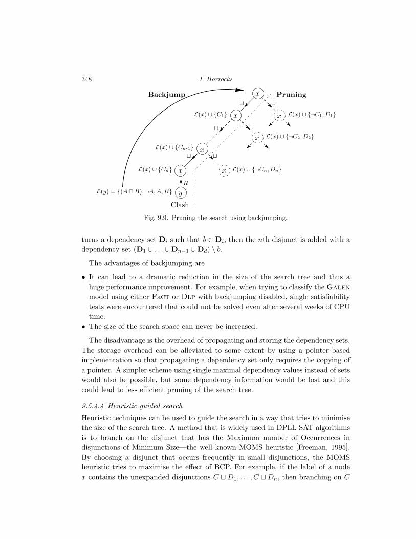
348 I. Horrocks

PruningBackjumpt

t

t

R

L(x) ∪ {C1} L(x) ∪ {¬C1, D1}

L(x) ∪ {¬C2, D2}

L(x) ∪ {Cn}

L(y) = {(A uB),¬A, A, B}

x

x

y

x

x L(x) ∪ {¬Cn, Dn}

t

t

tL(x) ∪ {Cn-1}

Clash

x

x

x

Fig. 9.9. Pruning the search using backjumping.

turns a dependency set Di such that b ∈ Di, then the nth disjunct is added with adependency set (D1 ∪ . . . ∪Dn−1 ∪Dd) \ b.

The advantages of backjumping are

• It can lead to a dramatic reduction in the size of the search tree and thus ahuge performance improvement. For example, when trying to classify the Galenmodel using either Fact or Dlp with backjumping disabled, single satisfiabilitytests were encountered that could not be solved even after several weeks of CPUtime.

• The size of the search space can never be increased.

The disadvantage is the overhead of propagating and storing the dependency sets.The storage overhead can be alleviated to some extent by using a pointer basedimplementation so that propagating a dependency set only requires the copying ofa pointer. A simpler scheme using single maximal dependency values instead of setswould also be possible, but some dependency information would be lost and thiscould lead to less efficient pruning of the search tree.

9.5.4.4 Heuristic guided search

Heuristic techniques can be used to guide the search in a way that tries to minimisethe size of the search tree. A method that is widely used in DPLL SAT algorithmsis to branch on the disjunct that has the Maximum number of Occurrences indisjunctions of Minimum Size—the well known MOMS heuristic [Freeman, 1995].By choosing a disjunct that occurs frequently in small disjunctions, the MOMSheuristic tries to maximise the effect of BCP. For example, if the label of a nodex contains the unexpanded disjunctions C tD1, . . . , C tDn, then branching on C


leads to their deterministic expansion in a single step: when C is added to L(x),all of the disjunctions are fully expanded and when ¬C is added to L(x), BCP willexpand all of the disjunctions, causing D1, . . . , Dn to be added to L(x). Branchingfirst on any of D1, . . . , Dn, on the other hand, would only cause a single disjunctionto be expanded.

The MOMS value for a candidate concept C is computed simply by counting thenumber of times C or its negation occur in minimally sized disjunctions. Thereare several variants of this heuristic, including the heuristic from Jeroslow andWang [Jeroslow and Wang, 1990]. The Jeroslow and Wang heuristic considers alloccurrences of a disjunct, weighting them according to the size of the disjunction inwhich they occur. The heuristic then selects the disjunct with the highest overallweighting, again with the objective of maximising the effect of BCP and reducingthe size of the search tree.

When a disjunct C has been selected from the disjunctions in L(x), a BCP max-imising heuristic can also be used to determine the order in which the two possiblebranches, L(x)∪{C} and L(x)∪{¬C}, are explored. This is done by separating thetwo components of the heuristic weighting contributed by occurrences of C and ¬C,trying L(x)∪{C} first if C made the smallest contribution, and trying L(x)∪{¬C}first otherwise. The intention is to prune the search tree by maximising BCP in thefirst branch.

Unfortunately, MOMS-style heuristics can interact adversely with the backjump-ing optimisation because they do not take dependency information into account.This was first discovered in the Fact system, when it was noticed that usingMOMS heuristic often led to much worse performance. The cause of this phe-nomenon turned out to be the fact that, without the heuristic, the data structuresused in the implementation naturally led to “older” disjunctions (those dependenton earlier branching points) being expanded before “newer” ones, and this led tomore effective pruning if a clash was discovered. Using the heuristic disturbed thisordering and reduced the effectiveness of backjumping [Horrocks, 1997b].

Moreover, MOMS-style heuristics are of little value themselves in description logicsystems because they rely for their effectiveness on finding the same disjuncts re-curring in multiple unexpanded disjunctions: this is likely in hard propositionalproblems, where the disjuncts are propositional variables, and where the number ofdifferent variables is usually small compared to the number of disjunctive clauses(otherwise problems would, in general, be trivially satisfiable); it is unlikely in con-cept satisfiability problems, where the disjuncts are (possibly non-atomic) concepts,and where the number of different concepts is usually large compared to the num-ber of disjunctive clauses. As a result, these heuristics will often discover thatall disjuncts have similar or equal priorities, and the guidance they provide is notparticularly useful.

350 I. Horrocks

An alternative strategy is to employ an oldest-first heuristic that tries to maximisethe effectiveness of backjumping by using dependency sets to guide the expansion[Horrocks and Patel-Schneider, 1999]. When choosing a disjunct on which to branch,the heuristic first selects those disjunctions that depend on the least recent branch-ing points (i.e., those with minimal maximum values in their dependency sets), andthen selects a disjunct from one of these disjunctions. This can be combined withthe use of a BCP maximising heuristic, such as the Jeroslow and Wang heuristic,to select the disjunct from amongst the selected disjunctions.

Although the BCP and backjumping maximising heuristics described above havebeen designed with semantic branching in mind they can also be used with syn-tactic branching. The oldest first heuristic actually selects disjunctions rather thandisjuncts, and is thus a natural candidate for a syntactic branching heuristic. BCPmaximising heuristics could also be adapted for use with syntactic branching, forexample by first evaluating the weighting of each disjunct and then selecting thedisjunction whose disjuncts have the highest average, median or maximum weight-ings.

The oldest first heuristic can also be used to advantage when selecting the orderin which existential role restrictions, and the labels of the R-successors which theygenerate, are expanded. One possible technique is to use the heuristic to select anunexpanded existential role restriction ∃R.C from the label of a node x, apply the∃-rule and the ∀-rule as necessary, and expand the label of resulting R-successor. Ifthe expansion results in a clash, then the algorithm will backtrack; if it does not,then continue selecting and expanding existential role restrictions from L(x) untilit is fully expanded. A better technique is to first apply the ∃-rule and the ∀-ruleexhaustively, creating a set of successor nodes. The order in which to expand thesesuccessors can then be based on the minimal maximum values in the dependencysets of all the concepts in their label, some of which may be due to universal rolerestrictions in L(x).

The advantages of using heuristics are

• They can be used to complement other optimisations. The MOMS and Jeroslowand Wang heuristics, for example, are designed to increase the effectiveness ofBCP while the oldest first heuristic is designed to increase the effectiveness ofbackjumping.

• They can be selected and tuned to take advantage of the kinds of problem thatare to be solved (if this is known). The BCP maximisation heuristics, for exam-ple, are generally quite effective with large randomly generated and hand craftedproblems, whereas the oldest first heuristic seems to be more effective when clas-sifying realistic KBs.


The disadvantages are

• They can add a significant overhead as the heuristic function may be expensiveto evaluate and may need to be reevaluated at each branching point.

• They may not improve performance, and may significantly degrade it.

– Heuristics can interact adversely with other optimisations, as was the case withthe MOMS heuristic and backjumping in the Fact system.

– When they work badly, heuristics can increase the frequency with which patho-logical worst cases can be expected to occur. For example, with problemsthat are highly disjunctive but relatively under-constrained, using a BCP max-imising heuristic to select highly constraining disjuncts can force backtrackingsearch to be performed when most random branching choices would lead rapidlyto a clash free expansion.

– The cost of computing the heuristic function can outweigh the benefit (if any).

• Heuristics designed to work well with purely proposition reasoning, such as theBCP maximising heuristics, may not be particularly effective with DLs, wheremuch of the reasoning is modal (it involves roles and sub-problems). There hasbeen little work on finding good heuristics for modal reasoning problems.

9.5.4.5 Caching satisfiability status

During a satisfiability check there may be many successor nodes created. Some ofthese nodes can be very similar, particularly as the labels of the R-successors for anode x each contain the same concepts derived from the universal role restrictionsin L(x). Considerable time can thus be spent re-computing the satisfiability ofnodes that have the same label. As the satisfiability algorithm only needs to knowwhether a node is satisfiable or not, this time is wasted. Moreover, when classifyinga KB, similar satisfiability tests may be performed many times, and may providefurther opportunities for the re-use of satisfiability results for node labels if theseare retained across multiple concept satisfiability tests.

If the expansion of existential value restrictions in the label of a node x is de-layed until all other expansion possibilities have been exhausted (as in the tracetechnique), then as each existential role restriction ∃R.C is expanded it is possi-ble to generate the complete set of concepts that constitute the initial label of theR-successor; this will consist of C plus all the concepts derived from universal rolerestrictions in L(x).1 If there exists another node with the same set of initial con-cepts, then the two nodes will have the same satisfiability status. Work need bedone only on one of the two nodes, potentially saving a considerable amount of1 This ordering is used in the trace technique to minimise space usage, and may by useful or even required

for effective blocking.

352 I. Horrocks

processing, as not only is the work at one of the nodes saved, but also the work atany of the successors of this node.

Care must be taken when using caching in conjunction with blocking as thesatisfiability status of blocked nodes is not completely determined but is simplytaken to be equal to that of the blocking node. Another problem with caching isthat the dependency information required for backjumping cannot be effectivelycalculated for nodes that are found to be unsatisfiable as a result of a cache lookup.Although the set of concepts in the initial label of such a node is the same asthat of the expanded node whose (un)satisfiability status has been cached, thedependency sets attached to the concepts that made up the two labels may not bethe same. However, a weaker form of backjumping can still be performed by takingthe dependency set of the unsatisfiable node to be the union of the dependency setsfrom the concepts in its label.

A general procedure for using caching when expanding a node x can be describedas follows.

(i) Exhaustively perform all local expansions, backtracking as required, untilonly existential value restrictions (if any) remain to be expanded.

(ii) If there are no unexpanded existential value restrictions in L(x), then returnthe satisfiability status satisfiable to the predecessor node.

(iii) Select (heuristically) an unexpanded existential role restriction from L(x),expanding it and any applicable universal role restrictions to create a newnode y with an initial label L(y) (or create all such nodes and heuristicallyselect the order in which they are to be examined).

(iv) If y is blocked, then its satisfiability status S is directly determined by thealgorithm (normally satisfiable, but may depend on the kind of cycle thathas been detected [Baader, 1991]).

(a) If S = satisfiable, then return to step (ii) without expanding L(y).(b) If S = unsatisfiable, then backtrack without expanding L(y). The

dependency set will need to be determined by the blocking algorithm.

(v) If a set equal to L(y) is found in the cache, then retrieve the associatedsatisfiability status S (this is called a cache “hit”).

(a) If S = satisfiable, then return to step (ii) without expanding L(y).(b) If S = unsatisfiable, then backtrack without expanding L(y), taking

the dependency set to be the union of the dependency sets attachedto the concepts in L(y).

(vi) If a set equal to L(y) is not found in the cache, then set L = L(y) and expandL(y) in order to determine its satisfiability status S.


(a) If S = satisfiable and there is no descendent z of y that is blocked byan ancestor x′ of y, then add L to the cache with satisfiability statusS and return to step (ii).

(b) If S = satisfiable and there is a descendent z of y that is blocked by anancestor x′ of y, then return to step (ii) without updating the cache.

(c) If S = unsatisfiable, then add L to the cache with satisfiability statusS and backtrack, taking the dependency set to be the one returnedby the expansion of L(y).

The problem of combining caching and blocking can be dealt with in a moresophisticated way by allowing the cached satisfiability status of a node to assumevalues such as “unknown”. These values can be updated as the expansion progressesand the satisfiability status of blocking nodes is determined. Such a strategy isimplemented in the Dlp system.

A further refinement is to use subset and superset instead of equality whenretreiving satisfiability status from the cache: if L(x) is satisfiable, then clearlyany L(y) ⊆ L(x) is also satisfiable, and if L(x) is unsatisfiable, then clearly anyL(y) ⊇ L(x) is also unsatisfiable [Hoffmann and Koehler, 1999; Giunchiglia andTacchella, 2000]. However, using sub and supersets significantly increases the com-plexity of the cache, and it is not yet clear if the performance cost of this addedcomplexity will be justified by the possible increase in cache hits.

The advantages of caching the satisfiability status are:

• It can be highly effective with some problems, particularly those with a repetitivestructure. For example, the Dlp system has been used to demonstrate thatsome of the problem sets from the Tableaux’98 benchmark suite are trivial whencaching is used (all problems were solved in less than 0.1s and there was littleevidence of increasing difficulty with increasing problem size). Without caching,the same problems demonstrate a clearly exponential growth in solution time withincreasing problem size, and the system was unable to solve the larger problemswithin the 100s time limit imposed in the test [Horrocks and Patel-Schneider,1999].

• It can be effective with both single satisfiability tests and across multiple tests(as in KB classification).

• It can be effective with both satisfiable and unsatisfiable problems, unlike manyother optimisation techniques that are primarily aimed at speeding up the detec-tion of unsatisfiability.


• Retaining node labels and their satisfiability status throughout a satisfiability

354 I. Horrocks

test (or longer, if the results are to be used in later satisfiability tests) involves astorage overhead. As the maximum number of different possible node labels is ex-ponential in the number of different concepts, this overhead could be prohibitive,and it may be necessary to implement a mechanism for clearing some or all of thecache. However, experiments with caching in the Dlp system suggest that this isunlikely to be a problem in realistic applications [Horrocks and Patel-Schneider,1999].

• The adverse interaction with dependency directed backtracking can degrade per-formance in some circumstances.

• Its effectiveness is problem dependent, and (as might be expected) is most evidentwith artificial problems having a repetitive structure. It is highly effective withsome of the hand crafted problems from the Tableaux’98 benchmark suite, it isless effective with realistic classification problems, and it is almost completely in-effective with randomly generated problems [Horrocks and Patel-Schneider, 1999].

• The technique described depends on the logic having the property that the sat-isfiability of a node is completely determined by its initial label set. Extend thetechnique to logics that do not have this property, for example those which sup-port inverse roles, may involve a considerable increase in both complexity andstorage requirements.

9.6 Discussion

To be useful in realistic applications, DL systems need both expressive logics andfast reasoners. Procedures for deciding subsumption (or equivalently satisfiability)in such logics have discouragingly high worst-case complexities, normally exponen-tial with respect to problem size. In spite of this, implemented DL systems havedemonstrated that acceptable performance can be achieved with the kinds of prob-lem that typically occur in realistic applications.

This performance has been achieved through the use of optimisation techniques,a wide variety of which have been studied in this chapter. These techniques canoperate at every level of a DL system; they can simplify the KB, reduce the num-ber of subsumption tests required to classify it, substitute tableaux subsumptiontests with less costly tests, and reduce the size of the search space resulting fromnon-deterministic tableaux expansion. Amongst the most effective of these optimi-sations are absorption and backjumping; both have the desirable properties thatthey impose a very small additional overhead, can dramatically improve typicalcase performance, and hardly ever degrade performance (to any significant extent).Other widely applicable optimisations include enhanced traversal, normalisation,lazy unfolding, semantic branching and local simplification; their effects are lessgeneral and less dramatic, but they too impose low overheads and rarely degrade


performance. Various forms of caching can also be highly effective, but they doimpose a significant additional overhead in terms of memory usage, and can some-times degrade performance. Finally, heuristic techniques, at least those currentlyavailable, are not particularly effective and can often degrade performance.

Several exciting new application areas are opening up for very expressive DLs,in particular reasoning about DataBase schemata and queries, and providing rea-soning support for the Semantic Web. These applications require logics even moreexpressive than those implemented in existing systems, in particular logics that in-clude both inverse roles and number restrictions, as well as reasoning with generalaxioms. The challenge for DL implementors is to demonstrate that highly optimisedreasoners can provide acceptable performance even for these logics. This may re-quire the extension and refinement of existing techniques, or even the developmentof completely new ones.

One promising possibility is to use a more sophisticated form of dependencydirected backtracking, called dynamic backtracking [Ginsberg, 1993], that pre-serves as much work as possible while backtracking to the source of a con-tradiction. Another useful approach, indicative of the increasing maturity ofexisting implementations, is to focus on problematical constructors and devisemethods for dealing with them more efficiently. Good examples of this canbe seen in the Racer system, where significant improvements in performancehave been achieved by using more sophisticated techniques to deal with domainand range constraints on roles (see Chapter 2 for an explanation of these con-structs) and qualified number restrictions [Haarslev and Moller, 2001c; 2001d;2001a].

Finally, it should be reemphasised that, given the immutability of theoretical com-plexity, no (complete) implementation can guarantee to provide good performancein all cases. The objective of optimised implementations is to provide acceptableperformance in typical applications and, as the definition of “acceptable” and “typ-ical” will always be application dependent, their effectiveness can only be assessedby empirical testing. Hopefully, the new generation of highly optimised DL systemswill demonstrate their effectiveness by finding more widespread use in applicationsthan did their predecessors.

implementation and optimisation techniquesgweddell/cs848/dlhb-09.pdf · ian horrocks abstract ......

Documents