implementation and performance analysis of …
TRANSCRIPT

University of Texas at TylerScholar Works at UT Tyler
Electrical Engineering Theses Electrical Engineering
Fall 10-31-2017
IMPLEMENTATION AND PERFORMANCEANALYSIS OF LONG TERM EVOLUTIONUSING SOFTWARE DEFINED RADIOKedar BhusalUniversity of Texas at Tyler
Follow this and additional works at: https://scholarworks.uttyler.edu/ee_grad
Part of the Electrical and Computer Engineering Commons
This Thesis is brought to you for free and open access by the ElectricalEngineering at Scholar Works at UT Tyler. It has been accepted forinclusion in Electrical Engineering Theses by an authorized administratorof Scholar Works at UT Tyler. For more information, please [email protected].
Recommended CitationBhusal, Kedar, "IMPLEMENTATION AND PERFORMANCE ANALYSIS OF LONG TERM EVOLUTION USING SOFTWAREDEFINED RADIO" (2017). Electrical Engineering Theses. Paper 32.http://hdl.handle.net/10950/609

Implementation and Performance Analysis of Long Term Evolution
using Software Defined Radio
by
KEDAR BHUSAL
A thesis submitted in partial fulfillmentof the requirements for the degree of
Master of Science in Electrical EngineeringDepartment of Electrical Engineering
Melvin Robinson, Ph.D., Committee ChairCollege of Engineering
The University of Texas at TylerJuly 2017


Acknowledgements
First and foremost, I would like to thank God for everything I ever received; for my
loving parents and siblings, for all my ingenious and supportive teachers, for all my
endearing friends and colleagues, and for my dearest Shraddha. I appreciate all their
contribution in making me who I am today and love them beyond all measures.
I am extremely thankful to my advisor, Dr. Melvin Robinson, Assistant Professor
of Electrical Engineering, at University of Texas at Tyler, for his unfaltering support
and guidance throughout the process. His prompt and concise directions were crucial
in indulging me deeper in the subject matter of the thesis and generating and impro-
vising on the key concepts alongside. It may be my work in the end but it would not
have been so without Dr. Robinson’s invigorating efforts.
I would like to acknowledge the support of Dr. Hassan El-Kishky, Associate Pro-
fessor and Chair of Electrical Engineering at University of Texas at Tyler and Dr.
Ron J. Pieper, Associate Professor of Electrical Engineering at University of Texas at
Tyler and am grateful to them for being part of my thesis committee and providing
me with their valuable suggestions and comments.
Lastly, I would like to dedicate this thesis to my late mother Mrs. Khageshwori
Bhusal (I will always be a part of you, miss you and love you) and my sister Ms. Gita
Bhusal (for being my mum after my mum).

Table of Contents
List of Tables . . . . . . . . . . . . . . . . . . . . . . . . . . . . . . . . . . . . iv
List of Figures . . . . . . . . . . . . . . . . . . . . . . . . . . . . . . . . . . . v
List of Terms . . . . . . . . . . . . . . . . . . . . . . . . . . . . . . . . . . . . vii
Abstract . . . . . . . . . . . . . . . . . . . . . . . . . . . . . . . . . . . . . . . xii
Chapter One: Introduction . . . . . . . . . . . . . . . . . . . . . . . . . . . . 1
1.1 Introduction . . . . . . . . . . . . . . . . . . . . . . . . . . . . . . . . 1
1.2 Wireless communication fundamentals . . . . . . . . . . . . . . . . . 1
1.2.1 Interference . . . . . . . . . . . . . . . . . . . . . . . . . . . . 2
1.2.2 Fading . . . . . . . . . . . . . . . . . . . . . . . . . . . . . . . 3
1.3 Evolution of Wireless Communication . . . . . . . . . . . . . . . . . . 4
1.3.1 First Generation (1G) . . . . . . . . . . . . . . . . . . . . . . 4
1.3.2 Second Generation (2G) . . . . . . . . . . . . . . . . . . . . . 4
1.3.3 Third Generation (3G) . . . . . . . . . . . . . . . . . . . . . . 5
1.3.4 Fourth Generation (4G) . . . . . . . . . . . . . . . . . . . . . 6
1.4 Motivation . . . . . . . . . . . . . . . . . . . . . . . . . . . . . . . . . 6
1.5 Organization of Thesis . . . . . . . . . . . . . . . . . . . . . . . . . . 7
Chapter Two: Long Term Evolution (LTE) . . . . . . . . . . . . . . . . . . . 8
2.1 Overview . . . . . . . . . . . . . . . . . . . . . . . . . . . . . . . . . . 8
2.2 LTE Downlink . . . . . . . . . . . . . . . . . . . . . . . . . . . . . . . 9
i

2.3 Orthogonal Frequency Division Multiplexing (OFDM) . . . . . . . . . 11
2.4 LTE Uplink . . . . . . . . . . . . . . . . . . . . . . . . . . . . . . . . 14
2.5 Single Carrier Frequency Division Multiplexing Access . . . . . . . . 16
Chapter Three: Software Defined Radio Background . . . . . . . . . . . . . . 19
3.1 Introduction . . . . . . . . . . . . . . . . . . . . . . . . . . . . . . . . 19
3.2 Evolution of SDR . . . . . . . . . . . . . . . . . . . . . . . . . . . . . 19
3.3 Features of SDR . . . . . . . . . . . . . . . . . . . . . . . . . . . . . . 22
3.3.1 Flexibility . . . . . . . . . . . . . . . . . . . . . . . . . . . . . 22
3.3.2 Reliability . . . . . . . . . . . . . . . . . . . . . . . . . . . . . 22
3.3.3 Consistency and Stability of Parameters . . . . . . . . . . . . 23
3.3.4 Upgradability . . . . . . . . . . . . . . . . . . . . . . . . . . . 23
3.3.5 Reusability . . . . . . . . . . . . . . . . . . . . . . . . . . . . 23
3.3.6 Re-Configurability . . . . . . . . . . . . . . . . . . . . . . . . 23
3.3.7 Enhanced Functionality . . . . . . . . . . . . . . . . . . . . . 23
3.3.8 Lower Cost . . . . . . . . . . . . . . . . . . . . . . . . . . . . 23
3.4 Uses/Benefits of SDR . . . . . . . . . . . . . . . . . . . . . . . . . . . 24
3.4.1 For Manufacturers . . . . . . . . . . . . . . . . . . . . . . . . 24
3.4.2 For Network Operators/Radio Service Provider . . . . . . . . 24
3.4.3 For User/Subscriber . . . . . . . . . . . . . . . . . . . . . . . 24
Chapter Four: GNU Radio . . . . . . . . . . . . . . . . . . . . . . . . . . . . . 26
4.1 Introduction . . . . . . . . . . . . . . . . . . . . . . . . . . . . . . . . 26
4.2 GNU Radio Companion . . . . . . . . . . . . . . . . . . . . . . . . . 26
4.3 Components of GNU Radio Companion . . . . . . . . . . . . . . . . . 27
Chapter Five: System Implementation and Performance Analysis . . . . . . . 29
5.1 Implementation of OFDM . . . . . . . . . . . . . . . . . . . . . . . . 29
ii

5.2 Implementation of SCFDMA . . . . . . . . . . . . . . . . . . . . . . . 31
5.3 Performance Simulation . . . . . . . . . . . . . . . . . . . . . . . . . 31
5.3.1 Performance in Different Channel Models . . . . . . . . . . . . 34
5.3.2 Peak to Average Power Ratio . . . . . . . . . . . . . . . . . . 36
5.3.3 Effect of PAPR . . . . . . . . . . . . . . . . . . . . . . . . . . 38
5.3.4 Comparison of PAPR between OFDMA and SCFDMA . . . . 39
5.3.5 BER Analysis between OFDMA and SCFDMA . . . . . . . . 44
Chapter Six: Conclusion and Future work . . . . . . . . . . . . . . . . . . . . 48
Bibliography . . . . . . . . . . . . . . . . . . . . . . . . . . . . . . . . . . . . 50
Appendices
Appendix A: GNU Radio Companion Code Example . . . . . . . . . . . . . . 53
A.1 Example Hello World Program on GNU Radio Companion . . . . . . 53
A.2 Creating a New Block . . . . . . . . . . . . . . . . . . . . . . . . . . 57
Appendix B: GNU Radio sample C++ program . . . . . . . . . . . . . . . . . 61
iii

List of Tables
Table 2.1 LTE Downlink Configuration . . . . . . . . . . . . . . . . . . . . . 10
Table 2.2 LTE Uplink Parameters for SC-FDMA Transmission . . . . . . . . 15
Table 3.1 SDR Forum tier definitions . . . . . . . . . . . . . . . . . . . . . . 20
Table 5.1 Parameters used during simulation for PAPR Comparison . . . . . 40
Table 5.2 Pedestrian test environment tapped-delay-line parameters . . . . . 45
Table 5.3 Vehicular test environment tapped-delay-line parameters . . . . . . 45
iv

List of Figures
Figure 1.1 Block Diagram of Communication System . . . . . . . . . . . . . 1
Figure 1.2 Multipath in wireless communication . . . . . . . . . . . . . . . . 2
Figure 2.1 3GPP release timeline . . . . . . . . . . . . . . . . . . . . . . . . 9
Figure 2.2 LTE downlink physical resource based on OFDM . . . . . . . . . 10
Figure 2.3 LTE Downlink Frame Structure . . . . . . . . . . . . . . . . . . . 11
Figure 2.4 Block Diagram of OFDMA . . . . . . . . . . . . . . . . . . . . . . 12
Figure 2.5 OFDM System . . . . . . . . . . . . . . . . . . . . . . . . . . . . 14
Figure 2.6 OFDM Symbol with CP . . . . . . . . . . . . . . . . . . . . . . . 14
Figure 2.7 Uplink (SCFDMA) frame structure . . . . . . . . . . . . . . . . . 15
Figure 2.8 SCFDMA slot structure . . . . . . . . . . . . . . . . . . . . . . . 15
Figure 2.9 Block Diagram of SC-FDMA . . . . . . . . . . . . . . . . . . . . 16
Figure 2.10 SCFDMA transmitter showing localized and distributed subcarrier
mapping . . . . . . . . . . . . . . . . . . . . . . . . . . . . . . . . 17
Figure 2.11 Subcarrier allocation methods for multiple users (3 users, 12 sub-
carriers, and 4 subcarriers per user) . . . . . . . . . . . . . . . . 18
Figure 3.1 SDR Timeline . . . . . . . . . . . . . . . . . . . . . . . . . . . . . 21
Figure 3.2 Multidimensional Aspects of Software Defined Radio . . . . . . . 25
Figure 4.1 GNU Radio Block Diagram . . . . . . . . . . . . . . . . . . . . . 27
Figure 4.2 GNU Radio Companion . . . . . . . . . . . . . . . . . . . . . . . 28
Figure 5.1 OFDMA Implementation In GNU Radio . . . . . . . . . . . . . . 32
Figure 5.2 SCFDMA Implementation in GNU Radio . . . . . . . . . . . . . 33
Figure 5.3 OFDMA in AWGN Channel . . . . . . . . . . . . . . . . . . . . . 36
Figure 5.4 SCFDMA in AWGN Channel . . . . . . . . . . . . . . . . . . . . 36
Figure 5.5 OFDMA in Rayleigh Channel . . . . . . . . . . . . . . . . . . . . 37
Figure 5.6 SCFDMA in Rayleigh Channel . . . . . . . . . . . . . . . . . . . 37
Figure 5.7 OFDMA in Rician Channel . . . . . . . . . . . . . . . . . . . . . 38
Figure 5.8 SCFDMA in Rician Channel . . . . . . . . . . . . . . . . . . . . . 39
Figure 5.9 Scope Plot of transmitted OFDMA Signal . . . . . . . . . . . . . 40
Figure 5.10 Scope Plot of transmitted SCFDMA Signal . . . . . . . . . . . . 40
v

Figure 5.11 Comparison between CCDF of PAPR for OFDMA & SCFDMA
with QPSK Modulation (M = 256, N = 64). . . . . . . . . . . . . 41
Figure 5.12 Comparison between CCDF of PAPR for OFDMA & SCFDMA
with 16QAM Modulation (M = 256, N = 64). . . . . . . . . . . . 41
Figure 5.13 Comparison between CCDF of PAPR for OFDMA & SCFDMA
with 64QAM Modulation (M = 256, N = 64). . . . . . . . . . . . 42
Figure 5.14 Comparison between CCDF of PAPR for OFDMA & SCFDMA
with QPSK Modulation (M = 512, N = 64). . . . . . . . . . . . . 42
Figure 5.15 Comparison between CCDF of PAPR for OFDMA & SCFDMA
with 16QAM Modulation (M = 512, N = 64). . . . . . . . . . . . 43
Figure 5.16 Comparison between CCDF of PAPR for OFDMA & SCFDMA
with 64QAM Modulation (M = 512, N = 64). . . . . . . . . . . . 43
Figure 5.17 BER comparison between OFDMA, IFDMA and LFDMA with
QPSK modulation in AWGN Channel . . . . . . . . . . . . . . . 46
Figure 5.18 BER comparison between OFDMA, IFDMA and LFDMA with
QPSK modulation in Pedestrian A Channel . . . . . . . . . . . . 46
Figure 5.19 BER comparison between OFDMA, IFDMA and LFDMA with
QPSK modulation in Vehicular A Channel . . . . . . . . . . . . . 47
Figure A.1 Dial tone generator implementation on GRC . . . . . . . . . . . . 53
Figure A.2 Demonstration of new block in GRC . . . . . . . . . . . . . . . . 59
Figure A.3 Result obtained by new block (square of triangular wave) . . . . . 60
vi

List of Terms
1G First Generation.
2G Second Generation.
3G Third Generation.
3GPP Third Generation Partnership Project.
4G Fourth Generation.
ADC Analog To Digital Converter.
AFRL Air Force Rome Labs.
AMPS Advanced Mobile Phone Systems.
BER Bit Error Rate.
BPSK Binary Phase Shift Keying.
C-CDF Complementary Cumulative Distribution Function.
CDF Cumulative Distribution Function.
CDMA Code Division Multiple Access.
COTS Commercial Off-The-Shelf.
CP Cyclic Prefix.
CRC Cyclic Redundancy Check.
DAC Digital To Analog Converter.
DARPA Defense Advanced Research Projects Agency.
vii

DFDMA Distributed Frequency Division Multiple Access.
DFT Discrete Fourier Transform.
DMR Digital Modular Radio.
DSP Digital Signal Processing.
E-UTRAN Evolved Universal Terrestrial Access Network.
EDGE Enhanced Data GSM Environment.
EPS Evolved Packet System.
EV-DO Evolution Data Optimized.
FDD Frequency Division Duplex.
FDMA Frequency Division Multiple Access.
FFT Fast Fourier Transform.
FM Frequency Modulation.
G Generation.
GPRS General Packet Radio Service.
GRC GNU Radio Companion.
GSM Global System Mobile.
GUI Graphical User Interface.
HR Hardware Radio.
HRPD High Rate Packet Data.
HSCSD High Speed Circuit Switched Data.
HSPA High-Speed Packet Access.
ICI Inter Channel Interference.
ICNIA Integrated Communications, Navigation, And Identification Architecture.
viii

IDFT Inverse Discrete Fourier Transform.
IEEE Institute Of Electrical And Electronics Engineers.
IFDMA Interleaved Frequency Division Multiple Access.
IFFT Inverse Fast Fourier Transform.
IMT International Mobile Telecommunications.
IS Interim Standard.
ISI Inter Symbol Interference.
ISR Ideal Software Radio.
ITU International Telecommunication Union.
LB Long Block.
LFDMA Localized Frequency Division Multiple Access.
LTE Long Term Evolution.
NMT Nordic Mobile Telephone System.
NTT Nippon Telephone And Telegraph Company.
OFDM Orthogonal Frequency Division Multiplexing.
OFDMA Orthogonal Frequency Division Multiple Access.
OOT Out Of Tree.
P/S Parallel To Serial.
PAPR Peak To Average Power Ratio.
PDC Pacific Digital Cellular.
PSK Phase Shift Keying.
QA Codes Quality Assurance Codes.
QAM Quadrature Amplitude Modulation.
ix

QPSK Quadrature Phase Shift Keying.
R8 Release 8.
R&D Research And Development.
RB Resource Blocks.
RE Resource Elements.
RF Radio Frequency.
RTT Radio Transmission Technology.
S/P Serial To Parallel.
SAE System Architecture Evolution.
SB Short Block.
SC-FDE Single Carrier-Frequency Domain Equalizer.
SC-FDM Single Carrier - Frequency Division Multiplexing.
SC-FDMA Single Carrier - Frequency Division Multiple Access.
SCR Software Controlled Radio.
SDR Software Defined Radio.
SNMP Simple Network Management Protocol.
SNR Signal To Noise Ratio.
SWIG Simplified Wrapper And Interface Generator.
TD-SCDMA Time Division Synchronous Code Division Multiple Access.
TDD Time Division Duplex.
TDMA Time Division Multiple Access.
UE User Equipment.
UMTS Universal Mobile Telecommunication System.
x

USR Ultimate Software Radio.
WCDMA Wideband Code Division Multiple Access.
WIMAX Worldwide Interoperability For Microwave Access.
xi

Abstract
Implementation and Performance Analysis of Long Term Evolution
using Software Defined Radio
KEDAR BHUSAL
Thesis Chair: Melvin Robinson, Ph.D.
The University of Texas at Tyler
July 2017
The overwhelming changes in the field of communication brought about need for high
data rates, which led to the development of a system known as Long Term Evolution
(LTE). LTE made good use of Orthogonal Frequency Division Multiplexing Access
(OFDMA) in its downlink and Single Carrier Frequency Division Multiplexing Access
(SCFDMA) in its uplink transmission because of their robust performance. These
multiple access techniques are the major focus of study in this thesis, with their
implementation in the LTE system.
GNU Radio is a software Defined Radio (SDR) platform. It comprises of C++
signal processing libraries. For user simplicity, it has graphical user interface (GUI)
known as GNU Radio Companion (GRC), to build a signal processing flow graph.
GRC translates any specific task flow graph to a python program which calls in-
built C++ signal processing blocks. By leveraging this feature and existing modules
in GRC, OFDMA and SCFDMA is implemented. In this study we made use of
existing OFDMA flow graph of GNU Radio to study the behavior of downlink and
general performing SCFDMA system was implemented with some modifications of
the existing GNU Radio blocks.
With the GNU Radio implementation, we tested the working mechanism of both
the systems. OFDMA is used in downlink for achieving high spectral efficiency and
xii

SCFDMA was introduced in uplink due to its low PAPR feature. These multiple
access schemes have to meet the requirement of high throughput with low BER and
PAPR, low delays and low complexity. In this thesis we are focused on evaluating
these multiple access techniques in terms of BER and PAPR with modulation tech-
niques like QPSK, 16-QAM and 64-QAM. Performance analysis part is performed in
MATLAB.
xiii

Chapter One
Introduction
1.1 Introduction
Wireless communication has always been a topic of extensive research. This research
has helped the field to grow exponentially in both applications and societal benefits.
Due to better technologies it has also become affordable and reliable.
Wireless communication began when Marconi demonstrated the ability of radio to
continuously communicate with sailing ships in 1897. Subsequently wireless commu-
nication has been rapidly adopted throughout the world. In 1946, the first American
public mobile telephone service was introduced with high power transmitters and
large towers covering a distance of 50km. Since then, mobile telephone service has
seen enhancements in hardware and software and these have led to the development
of modern telephony systems like 3G, UMTS and ultimately 4G/LTE [1].
1.2 Wireless communication fundamentals
Source Transmitter Channel Receiver Destination
Figure 1.1: Block Diagram of Communication System
Figure 1.1 shows a block diagram of communication system. Wireless communica-
tion provides a medium to transmit message from one place to another. The user in
the source, sends the message from transmitter through the channel, to the receiver
for the destination user. A channel can be defined as the path in which signal is
transmitted from one place to another. In traditional wired communication systems,
a channel is a guided medium or wire whereas in a wireless communication system
1

Figure 1.2: Multipath in wireless communication
a channel is unguided and uses electromagnetic waves to transmit messages. The
performance of wireless communication depends on the channel. The effects of a
channel and its realization is described in [2–5]. Unlike guided mediums, there are
certain disturbances in wireless communication which make the problem challenging
and interesting.
The path between the transmitter and receiver may vary in short span of time. It
can change from direct line of sight to one that takes several different paths caused by
obstruction such as buildings, trees or mountains. These disturbances are generally
reflection, diffraction and scattering. Reflection of a signal occurs when the signal
wave strikes a solid surface with size much longer than its wavelength, for example
a solid wall. Diffraction occurs when the signal strikes on the edges and corners
of a solid surfaces, like corners or edges of wall. When a signal travels through
a channel containing objects whose dimension is smaller than its wavelength, the
wave is scattered and the process is termed scattering. Reflection, diffraction and
scattering result in multipath propagation as in Figure 1.2 which is further responsible
for interference and fading. To be effective, wireless communication systems must be
designed to overcome to both interference and fading.
1.2.1 Interference
One of the major wireless communication problems is interference, which is broadly
defined as an unwanted modification of the signal as it traverses the path from the
2

base station to the user equipment (path referred to as the downlink channel) or from
the user equipment to the base station (path referred to as the uplink channel). A
major form of interference results from electromagnetic field scattering, reflection and
refractions from building and other surrounding objects. This is known as multipath
interference and it manifests itself as Inter Symbol Interference at the receiver. When
the signal travels from multiple path, one of the signal at line of sight is received first
and then other signals from reflected path with certain delays. These reflected signal
affects the subsequent signal. This unwanted phenomena in wireless communication
system is defined as Inter Symbol Interference.
1.2.2 Fading
Fading is a phenomenon in which a wireless channel experiences variation of chan-
nel strength over time and frequency. To understand the relation between channel
and multipath fading, we need to understand few more concepts. When the User
Equipment (UE) is moving there will be change in frequency, known as Doppler shift
(or Doppler spread). In a multipath channel, the received signal is superposition of
all the signal waves; direct from line of sight and other reflected waves. When the
phase difference between received signals is an integer multiple of 2π, signal adds
constructively and if the phase difference is an odd integer multiple of π, signal add
destructively degrading the quality [2].
It is also important to understand measures of signals coherence. Considering the
time domain, the length of time that a channel’s impulse response is assumed to be
constant is termed coherence time. It can also be defined as the time in which the
channel interference changes from constructive to destructive or vice versa. Consid-
ering the frequency domain, the bandwidth in which a channel’s impulse response
is assumed to be constant is defined as coherence bandwidth. Considering the spa-
tial domain, the distance between the transmitter and receiver in which the channel
remains same is known as coherence distance. At receiver there is certain delay in
receiving these signals. The difference between the time delays along two signal path
is called delay spread which is the reciprocal of coherence bandwidth.
A wireless communication channel’s coherence time classifies the channel as either
fast or slow fading. If the coherence time is much shorter than the delay requirement,
the channel is called a fast fading channel and if the coherence time is longer than
the delay requirement, the channel is called a slow fading channel.
A wireless communication channel’s coherence bandwidth classifies the channel as
either flat fading or frequency selective fading. The channel is said to be flat fading,
3

if the bandwidth of input signal is much smaller than the coherence bandwidth of the
channel. A channel is said to be frequency selective fading, if input signal bandwidth
is much larger than the coherence bandwidth .
1.3 Evolution of Wireless Communication
The cellular wireless generation (G) is a term used to keep track of the development
of transmission technology that incorporates all the changes in its nature of service,
non-backward compatibility and introduction of newer frequency bands. Its evolution
is commonly referred to as 1G, 2G, 3G and 4G, with each generation spanning roughly
a decade. Each generation had different features, addressing different issues, following
different evolutionary paths to achieve the unified goal of achieving high efficiency
and performance [1].
1.3.1 First Generation (1G)
The first generation (1G) used analog communication techniques (analog FM or FD-
MA/FDD) typically for speech services. In 1979, Nippon Telephone and Telegraph
Company (NTT) implemented world’s first the cellular system in Japan that used 600
FM duplex channels (23kHz for each one-way link) in the 800MHz band. In 1981, the
Nordic mobile telephone system (NMT 450) introduced the cellular mobile services
in Europe for 450MHz band and used 25kHz channels. In 1983, AMPS became the
first cellular telephone system to start services in the US with 666 duplex channels
with 40MHz of spectrum in the 800MHz band. These systems were highly inefficient
in terms of frequency spectrum usage as the individual cells were large and provided
low capacity and the mobile devices were large and expensive.
1.3.2 Second Generation (2G)
Introduced in the early 1990s, the second generation standards used digital modu-
lation formats and TDMA/FDD and CDMA/FDD multiple access techniques. The
most popular standards include:
(i) Global System mobile (GSM) - Used TDMA standard; supported 8-time slotted
users for each 200kHz radio channel; popular in Europe, Asia, Australia, South
America and some parts of US.
4

(ii) Interim Standard 136 (IS-136) - Used TDMA standard; supported 3 time slotted
users for each 30kHz radio channel; popular in North America, south America
and Australia.
(iii) Pacific Digital Cellular(PDC)- A Japanese TDMA standard; similar to IS-136.
(iv) Interim Standard 95 Code Division Multiple Access (IS-95 or cdmaOne)-Used
CDMA standard; supported up to 64 users that are orthogonally coded and sim-
ultaneously transmitted on each 1.25MHz channel; popular in North America,
Korea, Japan, China, South America and Australia.
While 2G offered higher spectrum-efficiency, better data services and advanced roam-
ing as compared to the 1G, it still could not support substantial data transmission
and speed. As a result, 2.5G devices were built by introducing the core network’s
packet switched domain and by modifying the air interface so that it could handle
both data and voice [6]. These provided upgrade options for each of the 2G stand-
ards: 3 for GSM (HSCSD, GPRS and EDGE) two of which also supported IS-136
and PDC (GPRS and EDGE) and 1 for IS-95(IS-95B).
1.3.3 Third Generation (3G)
In 3G systems, the air interface included extra optimization that were targeted at
data applications, which increased the average rate at which user could upload or
download information. The popular 3G technologies can be listed as:
(i) Universal Mobile Telecommunication System (UMTS): Most popular 3G system
is the UTMS, that was developed originally from GSM by completely changing
the technology used on the air interface while keeping the core network almost
unchanged and which went on to use the technology of high-speed packet access
(HSPA) for enhanced data application. The UTMS air-interface had two im-
plementations: Wideband code division multiple access (WCDMA) And Time
Division synchronous code division multiple access (TD-SCDMA). WCDMA se-
gregates the transmissions from base station and mobiles by means of frequency
division duplex, while TD-SCDMA uses time division duplex. WCDMA uses a
wide bandwidth of 5MHz and TD-SCDMA uses 1.6MHz only.
(ii) CDMA2000 1x radio transmission technology (1xRTT): CDMA2000 (1xRTT)
was developed from IS-95 originally that was further upgraded to cdma2000
high-rate packet data(HRPD) or evolution data optimized(EV-DO), that used
similar techniques as HSPA.
5

(iii) Worldwide Interoperability for Microwave Access(WiMAX): WiMAX was de-
veloped by IEEE under IEEE standard 802.16 and different from other 3G sys-
tems. In 2004, Third Generation Partnership Project (3GPP) began to study
into long term evolution of UMTS by modifying its architecture that resulted
in the LTE systems.
1.3.4 Fourth Generation (4G)
The International Telecommunication Union (ITU) published a set of requirements
for 4G under the name of International Mobile Telecommunications (IMT)-Advanced
that specifies that the, peak data rate of compatible system should be at least
600Mbps on the downlink and 270Mbps on the uplink, in the bandwidth of 40MHz.
Two systems met these requirements namely: LTE- Advanced and WiMAX 2.0. Al-
though, LTE and WiMAX 1.0 were both much advanced than other 3G systems,
these were considered as 3.9G due to the ITU guidelines. However, ITU later started
accepting these as a part of the 4G systems.
1.4 Motivation
In mobile communication, LTE is the latest technology to provide connectivity and
advanced services [7]. LTE achieves higher peak data rates up to 50 Mbps in uplink
and 100 Mbps in downlink with scalable bandwidth and better spectral efficiency.
All of this is achieved with using OFDMA for the downlink and SCFDMA for the
uplink.
Another important development in the field of communication is Software Defined
Radio (SDR). As a result of rapid adoption and growth, operators upgrade their
hardware with every generation of wireless communication. In many cases, these
upgrades require complete modification of the existing devices. This is costly and
constraints researchers, service providers and end-users. To address this limitation,
the concept of Software Defined Radio [8] was introduced, which reduces the need
of hardware replacement for each upgrade, which made it more affordable. Merely
changing the source is sufficient for and upgrade. As a result, SDR seems to have a
promising future in the field of wireless communication.
SDR has gained popularity in recent years and has been used as very efficient
and cost-effective means of studying several wireless technologies. It has allowed
researchers to implement wireless systems with greater flexibility and freedom [9].
By combining LTE and SDR technologies, we can analyze the performance of both
6

OFDMA and SCFDMA in terms of the key metrics PAPR and BER. PAPR is defined
as the ratio of peak signal power to the average signal power and BER is used to assess
the quality of the received signal.
The study of PAPR is important as it has it impacts on the overall power effi-
ciency of the system. It is also required to design RF transmitter power as power
amplifier at transmitter should be operated within the range of linearity to ensure
the removal/reduction of quantization noise.
BER, a measure of the quality of the received signal, is expressed in terms of Signal
to Noise Ratio (SNR) which is the ratio of signal power to the noise power in the
frequency range of operation. Generally, higher SNR values result in lower BER and
the system performance is said to better. Therefore, study of BER is used in wireless
communication system to determine the likelihood of receiving correct data.
SDR provides us with the toolkit to analyze these data over various constraints;
it lets us manipulate various parameters to study the behavior of any system. SDR
will be handy even as we move to 5G.
1.5 Organization of Thesis
This thesis use GNU Radio to study performance of a simulated LTE system. Chapter
2 provides background on the LTE (Long Term Evolution) system of wireless com-
munication. In Chapter 3, we introduce software defined radio (SDR), outline its
benefits and cover some modern implementations. In Chapter 4, we discuss one im-
plementation of software defined radio: GNU Radio, which is the major platform for
this research. In Chapter 5, we implement an LTE uplink and downlink system and
measure the performance of a data transmission system. The performance metrics are
probability of error at a given bit rate (BER) and the Signal-to-Noise Ratio (SNR).
Despite all of its advantages, OFDMA it is said to have high PAPR which is over-
come by SCFDMA. Accordingly, we investigate the BER performance of OFDMA
and SCFDMA systems as well we will compare the PAPR between these two systems
used in LTE. Finally, in Chapter 6, we conclude and present ideas for future work.
7

Chapter Two
Long Term Evolution (LTE)
2.1 Overview
Officially known as evolved packed system (EPS), LTE is a colloquial term used for
the system with two parts namely: system architecture evolution (SAE) and long
term evolution (LTE). SAE covered the core network whereas the LTE covered the
radio access network, air interface and mobile [2]. The Third Generation Partnership
Project (3GPP) produced specifications for LTE and is also responsible for manage-
ment of its successive versions and releases, as shown in Figure 2.1, which ensured
system compatibility and added functionality.
The 3GPP requirements LTE, dealing with air interface, specifies that it has to
deliver peak data rates of 100Mbps and 50Mbps respectively in downlink and uplink.
Also, it has to deal with the latency, for voice related applications. The time taken
for data to reach user equipment from fixed transmitter should be less than 5ms,
provided that the air interface is not congested. Mobile phones can operate either in
active mode or stand by mode and the switching time from standby state to active
state after user intervention should be less than 100ms. In addition to LTE, 3GPP
specifies SAE as a IP-based architecture which is required to support IP version 4,
IP version 6 or dual stack IPV4/IPV6. The main component of SAE is Evolved
Packet Core (EPC). EPC provide users always on connectivity by setting up a basic
IP connection as long as it is on in the network. EPC is responsible for controlling the
data rate, error rate and the data stream delays. Also, it is responsible for handover
between LTE and earlier 2G and 3G technologies.
LTE has demonstrated its importance as a versatile technology that meets the
requirement set by 3GPP. LTE can be deployed in flexible carrier bandwidths from
1.4MHz up to 20MHz. LTE also support different modes of operation, Time Division
Duplex (TDD) or Frequency Division Duplex (FDD). LTE has been able to provide
8

Figure 2.1: 3GPP release timeline
better, faster service to users whereas flexibility and efficiency of LTE has established
itself as a choice to network operators.
2.2 LTE Downlink
LTE or the E-UTRAN (Evolved Universal Terrestrial Access Network), introduced
in 3GPP R8, is the access part of EPS. The main advantage of an LTE network
is high spectral efficiency, high peak data rates, short round trip time as well as
flexibility in frequency and bandwidth. LTE downlink is based on OFDMA (Or-
thogonal Frequency Division Multiple Access). OFDMA in combination with higher
order modulation (up to 64QAM), large bandwidths (up to 20MHz) and spatial mul-
tiplexing in the downlink (up to 4x4) is able to achieve high data rates. The highest
theoretical peak data rate on the transport channel is 75 Mbps in the uplink, and
in the downlink, using spatial multiplexing, the rate can be as high as 300 Mbps.
For the uplink SCFDMA (Single Carrier Frequency Division Multiple Access) also
known as DFT (Discrete Fourier Transform) spread OFDMA is used [10]. SCFDMA
has inherited most of the OFDMA features and additionally overcomes the major
drawback of OFDMA to obtain a low PAPR. SCFDMA is preferred in uplink due to
low PAPR which secures low power consumption in the user devices.
LTE transmission on downlink is based on OFDM as it can transmit data with
large number of parallel, narrowband subcarriers along with the property of being
resilient to the slowly fading channel. The transmitted symbols are based on time-
9

Table 2.1: LTE Downlink Configuration
Transmission Bandwidth (MHz) 1.25 2.5 5 10 15 20Slot duration ms 0.5Sub-Carrier spacing (kHz) 15Number of RBs 6 12 25 50 75 100FFT Size 128 256 512 1024 1536 2048Number of occupied subcarriers 72 180 300 600 900 1200
Figure 2.2: LTE downlink physical resource based on OFDM [11]
frequency grid. Resource Element (RE) is one modulation symbol on one subcarrier,
which are combined to Resource Blocks (RBs) that are composed of twelve consec-
utive subcarriers and six or seven OFDM symbols as illustrated in Figure 2.2. The
number of OFDM symbols depends on the length of Cyclic Prefix (CP) i.e. normal or
extended. The LTE downlink configuration based on bandwidth and RBs are shown
in Table 2.1.
Figure 2.3 shows an LTE transmission frame. The duration of each frame is 10ms
that is composed of ten sub-frames. These sub-frames include two slots with each
of six or seven OFDM symbols depending on the length of cyclic prefix (normal or
extended). If we assume normal CP mode, then each slot will have seven OFDM
symbols and each sub-frame will have 14 OFDM symbols which sums up to 140
OFDM symbols in a frame. The total number of subcarriers is dependent on the
10

Figure 2.3: LTE Downlink Frame Structure
available bandwidth as listed in Table 2.1 which was taken from [12]. As explained,
all the LTE downlink systems are based on OFDM, we will further explain OFDM
transmission and reception.
2.3 Orthogonal Frequency Division Multiplexing (OFDM)
OFDM is a multicarrier modulation technique commonly used in communication
systems that require high data rates. This is due to its robustness in multipath
propagation. OFDM is a parallel transmission scheme, where a high-rate serial data
stream is split into a set of low-rate sub streams, each of which are modulated on a
separate subcarrier. The bandwidth of the sub-carriers becomes small compared with
the coherence bandwidth of the channel; that is, the individual sub-carriers experience
flat fading, which allows for simple equalization. This implies that the symbol period
of the sub streams is long when compared to the delay spread of the radio channel.
By selecting a set of carrier frequencies that are orthogonal, high spectral efficiency
is obtained because the spectra of the sub-carriers overlap, while mutual influence
among the sub-carriers can be avoided by introducing a guard period known by cyclic
prefix [13]. Figure 2.4 shows the block diagram of OFDMA. In OFDM transmission
first a sequence of QAM or PSK symbols with a symbol time are converted from
serial to parallel. Each of N symbols from serial to parallel conversion is carried out
by different sub-carrier. Let Xi[k] denote the ith transmitted symbol at kth subcarrier
where i ∈ Z+ and k ∈ {0, 1, 2, . . . , N − 1}. As the symbols are converted from serial
11

Figure 2.4: Block Diagram of OFDMA
to parallel the transmission time for N symbols is extended such that Tsym = NTs ,
where Tsym is the length of a single OFDM symbol. Let ψi,k(t) denote the ith OFDM
signal at the kth subcarrier, then,
ψi,k(t) =
ej2πfk(t−iTsym) 0 < t ≤ Tsym
0 elsewhere(2.1)
The passband and baseband OFDM signal in continuous time domain can be ex-
pressed as
x1(t) = Re
{1
Tsym
∞∑i=0
N−1∑k=0
Xi[k]ψi,k(t)
}(2.2)
and
x1(t) =∞∑i=0
N−1∑k=0
Xi[k]ej2πfk(t−Tsym) (2.3)
When the continuous time based OFDM signal in equation (2.3) is sampled at
t = iTsym + nTs with fk =k
Tsym, the results will be
x1[n] =N−1∑k=0
Xi[k]ej2πkn/N (2.4)
for n ∈ {0, 1, . . . , N − 1}Now, consider the received baseband OFDM symbol as,
yi(t) =N−1∑k=0
Xi[k]ej2πfk(t−iTsym), iTsym < t ≤ iTsym + nTs (2.5)
Two signals are defined to be orthogonal if the integral of their product over their
fundamental period is zero [14]. Using this feature of OFDM symbol Xi[k] can be
12

reconstructed as follows:
Yi[k] =1
Tsym
∫ ∞−∞
yi(t)e−j2πkfk(t−iTsym) dt (2.6)
=1
Tsym
∫ ∞−∞
{N−1∑m=0
Xi[m]ej2πfm(t−iTsym)
}e−j2πkfk(t−iTsym) dt
=N−1∑m=0
Xi[m]
{1
Tsym
∫ Tsym
0
ej2π(fm−fk)(t−iTsym)
}= Xi[k]
In the above realization, the effects of channel and noise are not considered. Let
{yi[n]}N−1n=0 be the sample values of the received OFDM yi(t) at t = iTsym + nTs.
Then, following the steps as in (2.6),
Yi[k] =N−1∑n=0
yi[n]e−j2πknN (2.7)
=N−1∑n=0
{1
N
N−1∑n=0
Xi[m]ej2πmnN
}e−
j2πknN
=1
N
N−1∑n=0
N−1∑m=0
Xi[m]ej2π(m−k)n/N = Xi[k]
Equation (2.4) is the N-point inverse Discrete Fourier Transform (IDFT) and (2.7)
gives the Discrete Fourier Transform (DFT). The DFT correlates each input signal
with the set of orthogonal sinusoids. If the input signal has some energy at a cer-
tain frequency k, it will be reflected at the correlation of the input signal and this
frequency, that is, in the value of spectrum for frequency . It means that the DFT con-
verts the time domain representation of the signal to the frequency domain. Whereas,
the IDFT converts signal spectrum, that is, frequency domain signal representation
to the time domain [15].
Thus, the OFDM system can be explained as such: modulated signal is passed to
serial-to-parallel converter which is input (frequency domain) for the IFFT block that
converts it to time domain blocks of symbols X[n]. These symbols are transmitted
over the channel. At receiver the time domain symbol is passed through the FFT
block which transforms to frequency domain and Y [k] is obtained after parallel-serial
processing. If the channel is noiseless the Y [k] coincides with X[k]. Figure 2.5
shows the OFDM system. But in wireless communication the presence of multipath
channel introduces ISI and ICI. When the received OFDM symbol is distorted by
the previously transmitted symbol, then the interference is known as ISI. Another
interference ICI occurs in such a way that the sub carrier may lose their orthogonality.
13

Figure 2.5: OFDM System
Figure 2.6: OFDM Symbol with CP
To overcome this problem, a guard interval of length Tg > Tc is added at the beginning
of each symbol where T > Tc is the channel time. The guard period (Cyclic Prefix)
is generated by duplicating the last Tg length of the symbol as shown in figure Figure
2.6.
2.4 LTE Uplink
In LTE uplink, transmission power consumption in UE terminals is a major concern.
Despite all the benefits of OFDM, the high PAPR limits its use in uplink transmission.
SC-FDM, a modified version of OFDM is introduced in uplink. It has similar through
put performance and complexity as in OFDM along with an advantage of low PAPR
[16]. Similar to downlink, uplink transmissions are segmented into frames. Each
frames consists of two sub frames which is further divided into two slots of 0.5ms
length. These slot contains 7 SCFDM symbols with normal CP. The generic frame
structure for SC-FDMA is shown in Figure 2.7 and the generic slot structure with
normal cyclic prefix is shown in Figure 2.8 [17]. The LTE uplink configuration is
shown in Table 2.2.
14
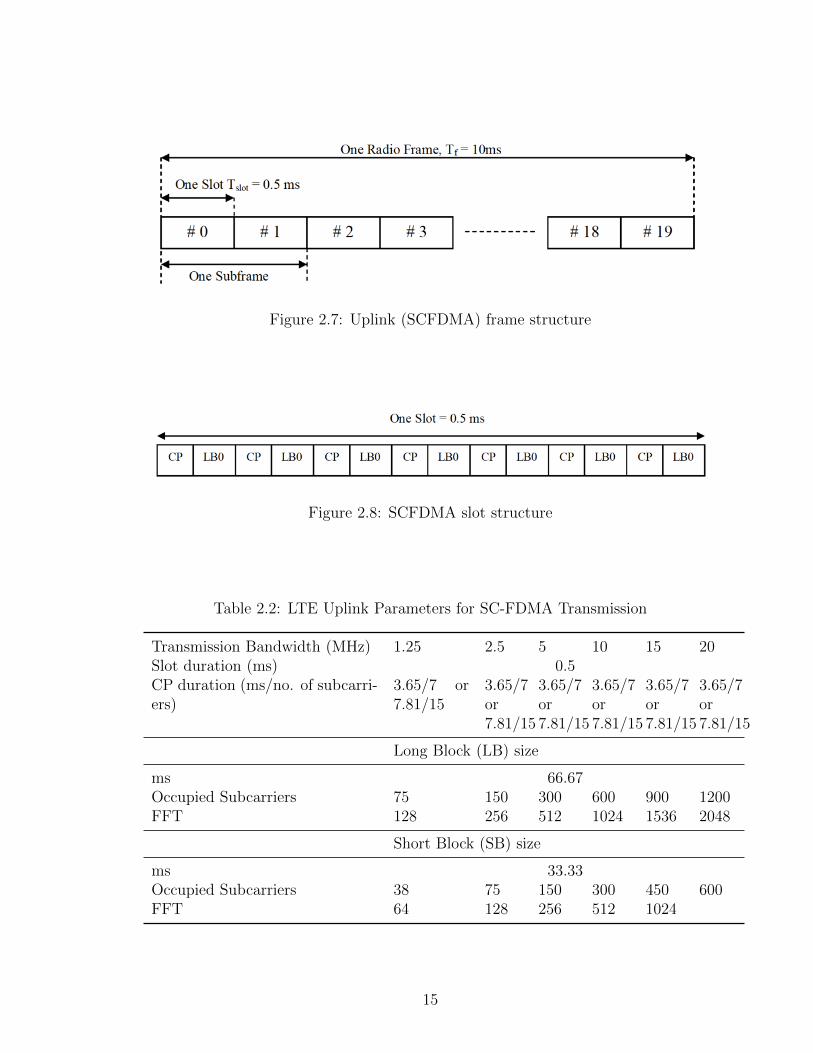
Figure 2.7: Uplink (SCFDMA) frame structure
Figure 2.8: SCFDMA slot structure
Table 2.2: LTE Uplink Parameters for SC-FDMA Transmission
Transmission Bandwidth (MHz) 1.25 2.5 5 10 15 20Slot duration (ms) 0.5CP duration (ms/no. of subcarri-ers)
3.65/7 or7.81/15
3.65/7or7.81/15
3.65/7or7.81/15
3.65/7or7.81/15
3.65/7or7.81/15
3.65/7or7.81/15
Long Block (LB) size
ms 66.67Occupied Subcarriers 75 150 300 600 900 1200FFT 128 256 512 1024 1536 2048
Short Block (SB) size
ms 33.33Occupied Subcarriers 38 75 150 300 450 600FFT 64 128 256 512 1024
15

Figure 2.9: Block Diagram of SC-FDMA
2.5 Single Carrier Frequency Division Multiplexing Access
SCFDMA is a multiple access technique that is built over OFDM modulation with
addition of a new DFT block before subcarrier mapping. A typical OFDM system uses
a large number of subcarriers contributing to a high PAPR, a major factor that led to
the development of SCFDMA, in which the overall transmit signal is a single signal,
which results in a low PAPR. SCFDMA is an extension of Single Carrier, Frequency
Domain Equalizer (SC-FDE) system that provides low PAPR due to single carrier
modulation at the transmitter, robustness to spectral null, lower sensitivity to carrier
frequency offset, and lower complexity at the transmitter which benefit the mobile
terminal in cellular uplink communications [18].
In SCFDMA, as in the block diagram shown in Figure 2.9, time domain data sym-
bols are transformed to frequency domain by DFT before going through OFDMA
modulation [18]. So, the only difference of SCFDMA from OFDM is the DFT block
because of which it is also known as DFT-OFDM. The transmitter of SCFDMA mod-
ulated symbols are grouped into blocks each containing N symbols. These symbols
are transformed into frequency domain by performing N -point DFT. Each of the
outputs obtained from N -point DFT are mapped to one of the M(M > N) ortho-
gonal sub carriers. M-point IDFT is performed to convert to a time domain signal.
Let Q be the maximum number of users that can transmit without any co-channel
interference then the output block size is given by M = QN . The transmitted then
adds CP to prevent the signal from interference.
At the receiver side, the reverse operations is performed. First, CP is removed
and the signal is transformed into frequency domain by performing M-point DFT.
After subcarrier de-mapping the equalized symbols are transformed back into the
time domain with N-point IDFT after which decoding and detection occurs to get
the transmitted signal.
16

Figure 2.10: SCFDMA transmitter showing localized and distributed subcarrier map-ping
In SCFDMA the transmission of subcarriers can be carried out in two ways; loc-
alized subcarrier mapping (referred to as Localized (L) - FDMA) and distributed
subcarrier mapping (referred to as Distributed (D) - FDMA). In the LFDMA mode,
the consecutive subcarriers are occupied by the DFT outputs of the input data and
in DFDMA mode, DFT outputs are distributed in subcarriers over the entire band-
width with zeroes assigned to the unused subcarriers. Interleaved FDMA (IFDMA) is
a special case of SCFDMA in DFDMA mode where the subcarriers are at equidistant
and without using DFT and IDFT, the transmitter can modulate the signal strictly
in the time domain, which makes it very efficient [19]. Figure 2.10 shows an SCF-
DMA transmitter with localized and distribute sub carrier mapping and Figure 2.11
shows the concept of subcarrier mapping in the frequency domain with an example
of 3 users, 12 subcarriers, and 4 subcarriers per user.
17

Figure 2.11: Subcarrier allocation methods for multiple users (3 users, 12 subcarriers,and 4 subcarriers per user)
18

Chapter Three
Software Defined Radio Background
3.1 Introduction
The term “Software Radio” was first coined by E-systems (now Raytheon) in a com-
pany newsletter in 1984. Then in 1991, DARPA’S SPEAKeasy became the first
military program that required its physical layer components to be implemented in
software. However, it was in 1992 that the very first paper on Software Radio was
published at IEEE National Telesystems Conference by Joseph Mitola. His paper
“Software Radio: Survey, Critical Analysis and Future Directions”, was so well re-
ceived that he is often referred to as the Godfather of Software Radio and is credited
to have coined the term “Software radio” despite the term being used by E-systems
previously for a prototype of a receiver [20].
Wireless innovation forum defined SDR as “Radio in which some or all, of the
physical layer functions are software defined” [21]. In brief ITU has defined SDR
as “A radio transmitter and/or receiver employing a technology that allows the RF
operating parameters including, but not limited to, frequency range, modulation
type, or output power to be set or altered by software, excluding changes to operating
parameters which occur during the normal pre-installed and predetermined operation
of a radio according to a system specification or standard” [22].
The SDR Forum, currently known by Wireless Innovation Forum, a non-profit
corporation that has been set up for development, deployment and use of open ar-
chitectures for advanced wireless systems, have also developed a 5 tier definition of
SDR [23] which are summarized in Table 3.1 below.
3.2 Evolution of SDR
SDR as we know today is convergence of various contemporary technologies that were
developed independently adding up to become one of the most remarkable break-
19

Table 3.1: SDR Forum tier definitions
Tier Name Description
0 Hardware Radio (HR) Baseline radio with fixed functionality1 Software-controlled radio (SCR) The radio’s signal path is implemented using
application-specific hardware, i.e., the signalpath is essentially fixed. A software interfacemay allow certain parameters, e.g., transmitpower, frequency, etc., to be changed in soft-ware.
2 Software defined radio (SDR) Much of the waveform, e.g., frequency, mod-ulation/demodulation, security, etc., is per-formed in software. Thus, the signal pathcan, with reason, be reconfigured in soft-ware without requiring any hardware modi-fications. For the foreseeable future, the fre-quency bands supported may be constrainedby the RF front-end.
3 Ideal software radio (ISR) Compared to a ’standard’ SDR, an ISR im-plements much more of the signal path in thedigital domain. Ultimately, programmabil-ity extends to the entire system with ana-logue/digital conversion only at the antenna,speaker and microphones.
4 Ultimate software radio (USR) The USR represents the ’blue-sky’ vision ofSDR. It accepts fully programmable trafficand control information, supports operationover a broad range of frequencies and canswitch from one air-interface/application toanother in milliseconds.
throughs in the history of radio communication. The first major contribution was
marked by development of Digital Signal Processing (DSP) techniques that basically
helped conversion of analog signal processes to digital processes. Newer techniques
were being developed within the DSP industry as well as separately by developers
who were developing software tools to provide modeling of the complex algorithms.
The Semiconductor industry also kept pace with these developments and provided
with matched computational performance for radio modulation and demodulation
to use digital signal processes. These developments caused exploration of various
machine learning techniques to help improve machine behavior, which were all some-
how helpful in evolution of the present day SDR. Furthermore, computer networking
20

Figure 3.1: SDR Timeline [24]
techniques were being developed commercially which soon evolved to wireless net-
working. Hence, we arrived to the era of SDR, which served as platform for first
adaptive radios then cognitive radios, all using digital signal processors and general
purpose processors built in silicon [24].
SDR software defines the properties of carrier frequency, signal bandwidth, modula-
tion, network access, cryptography, forward error correction coding and source coding
of voice, video or data. It is highly versatile and cost effective general purpose device
since the same radio tuner and processors can be used to implement many waveforms
at many frequencies and can be easily upgraded with new software for new waveforms
and new applications. However, in 1987, what is believed to be the first SDR device
was built when Air Force Rome Labs (AFRL) funded the integrated communications,
navigation, and identification architecture (ICNIA), a programmable modem, which
was a single box that housed a collection of single purpose radios. Then in 1990 AFRL
and Defense Advanced Research Projects Agency (DARPA) collectively funded the
SPEAKeasy I and SPEAKeasy II programs were the next major events in the history
of SDR.
SPEAKeasy I was heavily built radio that included a software programmable cryp-
tography chip called Cypress, with software cryptography developed by Motorola.
SPEAKeasy I demonstrated that a completely software programmable radio was in
fact possible and made way for SPEAKeasy II. SPEAKeasy II was portable sized and
gained popularity as the first SDR to include programmable voice coder, vocoder. It
21

was capable of handling different kinds of waveforms due to sufficient analog and DSP
resources and was constructed using standardized commercial off-the-shelf (COTS)
components which made it popular in defense equipment. SPEAKeasy II was so pop-
ular in the defense sector that it was used to create the US Navy’s digital modular
radio (DMR). DMR was a four channel full duplex SDR which could be remotely con-
trolled over Ethernet using Simple Network Management Protocol (SNMP). Both the
SPEAKeasy II and DMR had their importance to demonstrate that it was possible
to disintegrate the dependency of software on hardware components and vice versa
and could be developed independently. The modern SDR comprises of very advance
features capable of doing a great deal of computation. The SDR forum played a very
critical role in overall development of the field. SDR forum was founded in 1996 by
Wayne Bosner of AFRL to standardize SDR hardware and software for industries. It
was also important in standardizing porting software across various hardware plat-
forms, defining interfaces for multiple hardware vendors and facilitate integration of
software components from multiple vendors.
3.3 Features of SDR
The ongoing research and developments on SDR has proved it to be largely useful.
It seems to be widely applicable in various fields of communication because of its
features. Some of the generalized features are listed below.
3.3.1 Flexibility
With increased performance in PCs several tasks could be performed simultaneously.
This contributed in the progress of the SDR, making it more flexible, as all the
parameters of the system are configured on software unlike the traditional hardware
methods. It makes easier to use the similar hardware for different purpose by just
changing the guiding software.
3.3.2 Reliability
All the operations are done in software. Once compiled, there are little chance of
breakdown of software when compared to traditional hardware which makes the sys-
tem reliable. In case of error, it can simply be fixed with the modification of inherent
software.
22

3.3.3 Consistency and Stability of Parameters
Hardware and its performance are susceptible to the constraints such as weather
condition and aging whereas SDR seems to be consistent, stable and unaffected to
these constraints.
3.3.4 Upgradability
Upgrades are always possible with the changes or updates being in the software only,
which is cheaper and less time consuming than the hardware upgrades.
3.3.5 Reusability
Reusability is inherent feature of SDRs. The software programs are highly compatible
in similar hardware to perform similar operations, saving time and money.
3.3.6 Re-Configurability
The scope of tasks to be performed by SDR might differ with requirement of the
users which might change at any time. This can be achieved by simple modification
in software only which makes the system re-configurable.
3.3.7 Enhanced Functionality
With the control of software, it is much easier to provide an easy Graphical User
Interface (GUI) to control and verify the performance of a system. For one, SDR
platforms provides the functionality to incorporate newly introduced complex modu-
lation modes, making way for future technologies to use it, when needed, for various
aspects of design and development. All these features can be achieved using a general
purpose computer which is cheaper and provides all the functionality required.
3.3.8 Lower Cost
Change of hardware components become unnecessary since all the changes are being
carried out on software. The upgrades might also be less costly and latest technologies
could be employed in low budget projects as well.
23

3.4 Uses/Benefits of SDR
Traditional hardware based radio with low flexibility and higher cost can be easily re-
placed with flexible, efficient and inexpensive SDR providing multiband, multimode,
multicarrier and variable bandwidth characteristics. SDR provides the software con-
trol of variety of modulation making it usable on varieties of application. Its benefits
can be classified for the following:
3.4.1 For Manufacturers
For manufacturers, research and development takes considerable time and effort.
With reduced hardware, they can devote most of their resources to software de-
velopment which is reusable and reconfigurable as required. This saves a lot of time
and resources and can be done in a stepwise process by fixing bugs and proceeding
to new steps. Once developed it is much easier to do a mass production. Even more,
SDR helps them in providing after sales support as it can be done remotely thus
reducing the time and maintenance cost.
3.4.2 For Network Operators/Radio Service Provider
The main advantage of SDR for operators is that, they can roll out their services
within short period of time with reduced cost in logistics and implementation. Also,
the radio parameters are software configurable which helps in rapid development and
upgrades that are mainly advantageous over the costly base stations.
3.4.3 For User/Subscriber
End users can have two-way communication with whom they want and in any com-
munication systems. Also, they can have the possibility to change the carrier and take
advantage of worldwide mobility. Even the end user terminals can be reconfigured
according to the needs. However, the usage can best also be summarized with the
Figure 3.2 below.
24

Figure 3.2: Multidimensional Aspects of Software Defined Radio
25

Chapter Four
GNU Radio
4.1 Introduction
GNU Radio is an evolving open source development toolkit and is used for signal
processing. It is a powerful SDR platform with many signal processing and general
purpose blocks used in radio systems. Filters, decoders, modulators, encoders are
some commonly used blocks in GNU. The GNU Radio applications use both the
Python and C++ , where each serve different purposes. GNU Radio applications
are primarily written using the Python whereas C++ is used to create the complex
signal processing blocks. The connection between these two different programming
language is made possible with the use of SWIG (Simplified Wrapper and Interface
Generator), an open source software which generates a ‘glue code’ that enables calling
C++ functions from a Python programming language. Figure 4.1 gives a clear picture
of organization of data flow on GNU Radio.
GNU Radio is based on flow graphs and blocks concept. Blocks are basic operation
units that process continuous data streams and each block has a number of input and
output ports. There are different types of blocks already available and a new block
can also be created if required. The flow graphs are the composed of different blocks
through which the data flows. It means different blocks are arranged and connected
like a path of signal flow. These flow graphs can be written in either C++ or Python.
Each of these flow graphs require one source and sink for successful execution.
4.2 GNU Radio Companion
GNU Radio Companion (GRC) is a GUI tool for creating signal flow graphs and gen-
erating flow-graph source code [25]. GRC makes it easier to use GNU Radio features
with reduced programming but the degrees of freedom is certainly compromised when
compared to programming. On the other hand, it provides some variable blocks that
26

Figure 4.1: GNU Radio Block Diagram
can be used to pass variable values and also import some Python functions. GRC is
bundled with GNU Radio source and uses Cheetah templates to generate the Python
source code for the flow graph. It can generate source code for WX GUI, Qt and
non-GUI flow graphs as well as hierarchical blocks. It can also extract documentation
for gnu radio blocks from Doxygen-related XML files and also provides the definition
for the blocks present on GNU Radio. GRC can create hierarchical blocks out of built
in blocks and even lets us perform actions like enable, disable, cut, paste etc. GRC
comes to be handier as it can show the errors on the flow graphs before execution.
Figure 4.2 is the picture of the working area of the GNU Radio Companion. The
big central area is for creating the flow graph and is known as workspace. On the side
there are list of blocks, a library, that can be used to create a flow graph. On the top
it has toolbar to perform the desired actions and in the bottom pane is the terminal,
that shows the related messages that could be the output or any errors/warnings.
4.3 Components of GNU Radio Companion
Below are the components of GRC (GNU Radio Companion)
1. Flow Graph: GRC comprises of a scrollable window for creating an intercon-
nection of signal processing blocks known as flow graph.
2. Signal Blocks: These are the signal processing blocks in the flow graph. They
27

Figure 4.2: GNU Radio Companion
appear as rectangular blocks in the GRC with individual labels (comprising of
name and list of parameters) and can be a filter, an adder, a source or a sink.
3. Parameters: Parameters are the input to the function performed by the signal
blocks. Displayed below the label, a parameter can be a sampling rate, gain or
a flag.
4. Sockets: Each signal block has certain inputs and outputs associated with it
that are known as sockets. They appear as small rectangle attached to the
signal block and has a label that indicates its function.
5. Connections: An input socket and an output socket are joined using connec-
tions that are represented by a simple line between the sockets in the GRC. A
connection needs to be made within same data types.
6. Variables: It is simply a value or a number that can be accessed by all the
elements of the flow graph. These could be used to define the value of certain
parameter or could be used as a range of values to be dynamically changed to
observe certain characteristics while the flow graph is running.
28

Chapter Five
System Implementation and Performance Analysis
Previous chapters described the theory of LTE uplink and downlink and described
GNU Radio as well. This chapter will be focused on the implementation in GNU Ra-
dio. Also, we compare performance between OFDMA and SCFDMA using measures
BER and PAPR.
5.1 Implementation of OFDM
Figure 5.1 shows the flow graph of OFDMA implemented on GNU Radio. Various
blocks are used to perform transmission and reception. All the blocks used in the
flow graph are described in this chapter. File Source block reads raw data values in
binary format from the specified file. File saved with randomly generated sequence of
0s and 1s using random source generator provided in GNU Radio is used as input to
this source. There are several virtual sinks used to connect the flow graphs virtually.
These blocks are handy to make the flow graph tidy. All other major blocks are
explained as follows:
1. Stream to Tagged Stream: This built in block of GNU Radio converts regular
stream into a tagged stream. It adds length tags in regular intervals of stream.
2. Stream CRC32: The tagged stream of signal is passed to this block which
generates and adds 4-byte Cyclic Redundancy Check (CRC) to the end of the
data packets.
3. Protocol Formatter: This block is used to generate a packet header. The packet
header contains packet length (12 bits), packet ID (12 bits) and 8 bit CRC at the
end. Bits 0-11 gives the packet length, bits 12-23 indicates the header number
and bits 24-31 is an 8-bit CRC.
29

4. Repack Bits: As the name suggests, this block repacks k bit from input stream
into l bits of output stream where k and l can have values within [1,8]. In this
thesis, the header bits are mapped using BPSK and payload bit are mapped
using QPSK. So, this block converts every 1 bit into an integer from 0 to 1 is
BPSK and every 2 bits into an integer from 0 to 3 in QPSK used for header
and payload respectively.
5. Chunks to Symbol: This block maps a stream of unpacked symbols indexes to
stream of float or complex points. For the header bits, the integer from 0 to 1
are mapped to BPSK symbol and for the payload bits, the integer from 0 to 3
are mapped to QPSK symbols.
6. Tagged Stream Mux: This built-in block is used to merge two inputs namely
header bits and payload bits. Basically this block takes N streams of input with
certain packet length tags and outputs a signal with new tag which is sum of
all individual tags (of input stream).
7. OFDM Carrier Allocator: This block is used to create a frequency domain
OFDM symbols which is input to the IFFT. This block also adds pilot symbols
to each subcarrier. Also, two synchronization words for timing synchronization
and frequency offset estimation are added in this block.
8. FFT: With this block FFT operation is performed to change the symbols from
time domain to frequency domain and vice versa. If reverse FFT (IFFT) is
performed, then the frequency domain signal is transformed to time domain
and if forward FFT is performed then the time domain symbols are transformed
into frequency domain symbols.
9. OFDM Cyclic Prefixer: This block adds CP to the symbol. The length of CP is
defined as quarter of FFT length (which is equal to the number of subcarriers).
10. Schmidl&Cox OFDM Synchronization: This is built in block in GNU Radio
based on theory defined in [26] used for signal synchronization and frequency
correction. In order to detect the start symbol of a packet transmitted, this
block relies on the frame equalizer which calculates the timing metric, determ-
ines the start of the packet and informs next block with a trigger.
11. Header/Payload Demux: This block plays major role in receiver end of OFDM
system. It plays vital role in detecting header stream and payload stream.
30

Based on the trigger from Schmidl&Cox OFDM Synch block it will first detect
the outer header format. Then it will use the parsed outer header information
to detect the payload data.
12. OFDM Channel Estimation: This block is used to estimate frequency offset and
channel taps. The output of this block is a data symbol without synchronization
words which are send to other blocks by tags.
13. OFDM Frame Equalizer: This block performs equalization on a tagged OFDM
frame. One connected in the flow of header stream equalizes the outer header
stream and passes symbols to serializer while the other one connected to the
payload stream flow graph does the task of separating the packet corresponding
to the respective subcarriers. After this block, OFDM symbols are equalized
and frequency corrected.
14. OFDM Serializer: This block is used to convert parallel stream of data to serial.
15. Packet Header Parser: This block can be compared as inverse to the packet
header generator block. The output of this block is not the stream of data but
is a smart pointer dictionary used to figure out the index of subcarriers with
the same packet ID.
5.2 Implementation of SCFDMA
Figure 5.2 shows SCFDMA implementation in GNU Radio. As SCFDMA is modified
from OFDMA, only few other blocks are added to complete the implementation.
There is additional FFT and IFFT block (as described in theory with FFT size
N < M). SCFDMA Carrier Allocator block is a block that performs similar task
as in OFDMA but it does not add pilot symbols, pilot carriers and synchronization
words. Basically, it is used to map serial data to parallel. The block SCFDMA
Interleaver plays a vital role in distributing the data symbol to larger set of subcarrier
which is based on distributed mapping. Another additional block is SCFDMA frame
equalizer block used for frame equalization and symbol decision block is used to
convert complex signal to binary to prepare it for constellation mapping.
5.3 Performance Simulation
Theoretically, OFDMA and SCFDMA are quite effective in supporting the LTE re-
quirements. However, to verify the robustness of these systems perform different
31

Figure 5.1: OFDMA Implementation In GNU Radio
32

Figure 5.2: SCFDMA Implementation in GNU Radio
33

tests using GNU Radio and to support the results we performed those simulations in
MATLAB as well.
5.3.1 Performance in Different Channel Models
In simple terms, wireless channels can be defined as a path through which wireless
signal travels from transmitter to the receiver by means of electromagnetic radiation.
It is simply taken as the medium to transport, however, it is necessary to know the
complexity comprised in the channel to successfully decode the information at the
receiver. As channels are not solid medium, there are lots of obstructions basically
known by multipath effect, shadowing effect and time varying characteristics. To
distinguish the fading characteristics of the channel, particularly two distinct scen-
arios are taken in to consideration. The slow fading channel in which the channel
stays the same (random value) over the entire time-scale of communication and the
fast fading channel, where the channel varies significantly over the time scale of com-
munication [2]. It is a general practice in wireless communication to perform the
performance measure in these fading channel comparing with the non-faded Addit-
ive White Gaussian Noise (AWGN) channel. To demonstrate the multipath fading,
Rayleigh and Rician distribution can be considered to model a channel. GNU Ra-
dio consists of Rayleigh and Rician fading model blocks based on Random Walk
Process [27], as informed in documentation tab of the block.
1. AWGN Channel: AWGN is the most common channel model used in wireless
communication. In an AWGN channel, the signal is degraded by white noise η
which has a constant spectral density and a Gaussian distribution of amplitude.
The Gaussian distribution has a probability density function (pdf) given by [28]
P (r) =1√
2πσ2exp
(− r2
2σ2
)(5.1)
where σ2 is is the variance of Gaussian Random Process.
In AWGN, the signal at the receiver is the total of transmit signal and noise,
where the noise is statistically independent of the signal.
2. Rayleigh Channel: It is commonly used to describe the statistical time vary-
ing nature of the received envelope of a flat fading signal, or the envelope of an
individual multipath component [1]. This channel model represents the signal
transmission in environment with no line of sight (LOS) between transmitter
34

and receiver, that is common in heavily-built urban environment. The pdf for
Rayleigh channel is given by
P (r) =r
σ2exp
(− r2
2σ2
)(5.2)
where 0 ≤ r ≤ ∞ is envelope amplitude of received signal
3. Rician Channel: If there is a presence of strong dominant signal component,
like LOS, then the channel model is described as Rician Channel. It is similar
to Rayleigh channel except the LOS path of signal. The Rician distribution is
given by [2]
P (r) =r
σ2exp
(−r
2 + A2
2σ2
)I0
(Ar
σ2
)(5.3)
Where A denotes peak amplitude of dominant signal and A, r ≥ 0. The Rician
distribution commonly described by Rician Factor, K is gives by
K =A2
2σ2(5.4)
K(dB) = 10 log10
A2
2σ2(5.5)
Figure 5.3 shows the power spectral density (PSD) plot of OFDMA in AWGN channel.
PSD is the frequency response of a periodic or random signal and tells us where the
average power is distributed as a function of frequency [29]. Figure 5.3 (a) is the
signal received at receiver when the noise is 0dB and Figure 5.3 (b) is when the noise
is 10dB. From these two figures we observe that as the noise amplitude increases,
there is degradation in received spectrum amplitude. It means that, as the signal
transmits from transmitter to receiver, it degrades with the increase in separation
distance between them. As shown in Figure 5.4 SCFDMA performs similarly to
OFDMA.
Figure 5.5 and Figure 5.6 shows the performance of OFDMA and SCFDMA re-
spectively in Rayleigh fading distribution with normalized Doppler of 0.1 and 1.
Several test between 0.1 and 1 were performed for each system. It is clear that in
both the techniques, OFDMA and SCFDMA, the amplitude of the signal at receiver
remained same. Figure 5.7 and Figure 5.8, represents OFDMA and SCFDMA signal
that are passed through Rician Channel with Rician Factor (k) having values 0 and
5 and normalized maximum doppler of 0.1 and 1 in both the cases. It is seen that
they have similar performance in any scenarios. This demonstrates the robustness of
OFDMA and SCFDMA in the fading channel.
35

Figure 5.3: OFDMA in AWGN Channel
Figure 5.4: SCFDMA in AWGN Channel
5.3.2 Peak to Average Power Ratio
The PAPR occurs when in a multicarrier system the different sub-carriers are out
of phase with each other. At each instant they are different with respect to each
other at different phase values. When all the points achieve the maximum value
simultaneously; this will cause the output envelope to suddenly shoot up which causes
a ‘peak’ in the output envelope. Thus the ratio of peak signal power over the average
signal power is defined as PAPR [30]. Mathematically it is expressed as
PAPR =max |x(t)|2
E[|x(t)|2](5.6)
where |x(t)| is the magnitude of x(t) and E[.] denotes the expectation operator. The
cumulative distribution function (CDF) of the PAPR is one of the most frequently
used performance measures for PAPR reduction techniques. The complementary
36

Figure 5.5: OFDMA in Rayleigh Channel
Figure 5.6: SCFDMA in Rayleigh Channel
CDF (CCDF) is commonly used instead of the CDF itself. The CCDF of the PAPR
denotes the probability that the PAPR of a data block exceeds a given threshold [31].
The CDF of the amplitude of the signal is given by,
F (z) = 1− e−z (5.7)
The CCDF measures the probability of signal PAPR exceeding certain threshold.
Thus the CCDF of the PAPR of a data block is given by [31],
P (PAPR > z) = 1− P (PAPR ≤ z) = 1− F (z)N (5.8)
= 1− (1− e−z)N
37

Figure 5.7: OFDMA in Rician Channel
5.3.3 Effect of PAPR
The major effect of PAPR is reduction of overall power efficiency of the system. The
RF power amplifiers at the Transmitter should be operated specifically within a large
range of linearity, since the signal in the non-linear region suffers major distortion
leading to intermodulation amongst the subcarriers and out of band radiation. This,
however cannot be sustainable for wireless communication as it reduces the power
efficiency of the overall system. Additionally, the ADCs or DACs also need to be
operated in a wide working range in order to ensure elimination or reduction of any
quantization noise, which again increases the complexity of the system which is highly
undesirable. Despite the fact that a lot of techniques were proposed over the years
for reduction of PAPR in OFDMA, none were successful in providing any significant
results.
38

Figure 5.8: SCFDMA in Rician Channel
5.3.4 Comparison of PAPR between OFDMA and SCFDMA
From Figure 5.9 and Figure 5.10, we can observe that the peak power of an OFDMA
system is much greater than the average power of the system, whereas the maximum
peak power of SCFDMA system is within a close range of the average power. This
proves that the SCFDMA system has less PAPR than OFDMA system. To clarify
this, we have simulated the system in MATLAB with following parameters shown in
Table 5.1.
Simulation is performed with various types of modulation techniques along with
different number of subcarriers. In every simulation results it is clearly visible that
the PAPR of SCFDMA is better than the PAPR of OFDMA.
39

Figure 5.9: Scope Plot of transmitted OFDMA Signal
Figure 5.10: Scope Plot of transmitted SCFDMA Signal
Table 5.1: Parameters used during simulation for PAPR Comparison
Number of total Subcarrier (M) 256/512 Oversampling Factor 4Data Block Size (N) 64 Number of Iterations 1000System Bandwidth 5MHz
Modulation FormatQPSK
16 QAM64 QAM
40

4 6 8 10
10−3
10−2
10−1
100
PAPR[dB]
Pr[PAPR>PAPR
0]
SCFDMAOFDMA
Figure 5.11: Comparison between CCDF of PAPR for OFDMA & SCFDMA withQPSK Modulation (M = 256, N = 64).
4 6 8 10
10−3
10−2
10−1
100
PAPR[dB]
Pr[PAPR>PAPR
0]
SCFDMAOFDMA
Figure 5.12: Comparison between CCDF of PAPR for OFDMA & SCFDMA with16QAM Modulation (M = 256, N = 64).
41

4 6 8 10
10−3
10−2
10−1
100
PAPR[dB]
Pr[PAPR>PAPR
0]
SC-OFDMAOFDMA
Figure 5.13: Comparison between CCDF of PAPR for OFDMA & SCFDMA with64QAM Modulation (M = 256, N = 64).
4 6 8 10
10−3
10−2
10−1
100
PAPR[dB]
Pr[PAPR>PAPR
0]
SCFDMAOFDMA
Figure 5.14: Comparison between CCDF of PAPR for OFDMA & SCFDMA withQPSK Modulation (M = 512, N = 64).
42

4 6 8 10
10−3
10−2
10−1
100
PAPR[dB]
Pr[PAPR>PAPR
0]
SCFDMAOFDMA
Figure 5.15: Comparison between CCDF of PAPR for OFDMA & SCFDMA with16QAM Modulation (M = 512, N = 64).
4 6 8 10
10−3
10−2
10−1
100
PAPR[dB]
Pr[PAPR>PAPR
0]
SCFDMAOFDMA
Figure 5.16: Comparison between CCDF of PAPR for OFDMA & SCFDMA with64QAM Modulation (M = 512, N = 64).
43

5.3.5 BER Analysis between OFDMA and SCFDMA
Bit Error Rate (BER) is a performance parameter used to assess data quality of a
transmitted signal in wireless communication system. It is responsible for assessing
the performance of an overall system and is inclusive of transmitter, receiver and
the medium of transmission and when in operation. BER can be defined as rate at
which error occurs in a transmission system; which is simply a measure of received
bits that may have suffered deterioration/degradation mainly due noise and changes
in propagation path. Mathematically
BER =Bits in Error
Total Bits Received(5.9)
With the context of BER, Signal to Noise Ratio (SNR) is also considered. SNR is
the ratio of signal power to the noise power in the frequency range of the operation.
Noise power is due to unwanted signals present in the environment. BER is inversely
related to SNR. Thus a system with high Signal to Noise ratio (SNR) will have a
very low BER and vice versa. SNR is commonly used to evaluate the quality of a
communication link and is expressed as
SNR = 10 log10
Signal Power
Noise Power(5.10)
BER is often expressed in terms ofEbN0
, Energy per bit to Noise power spectral
density ratio, also known as SNR per bit which is used to compare BER of digital
system without taking bandwidth into consideration. Eb represents the energy in
one bit and N0 refers to the noise power spectral density (or noise power in 1Hz
bandwidth). Like BER it is dimensionless.
Figure 5.17 shows the BER performance of OFDMA, LFDMA and IFDMA and as
expected, in AWGN channel without multipath fading all of them exhibit the same
characteristics. Figure 5.18 and Figure 5.19 compares BER performance between
OFDMA, IFDMA and LFDMA with QPSK modulation in Pedestrian A channel
and Vehicular A channel with the parameters provided in Table 5.2 and Table 5.3
respectively.
From both figures, we can see that the IFDMA has a better performance com-
pared to LFDMA and OFDMA. In Pedestrian A channel all 3 techniques seem to
be performing with same characteristics however with the increase in SNR, IFDMA
and LFDMA seems to perform better than OFDMA. In Vehicular A channel OFDM
has better performance than SCFDMA techniques initially, however with higher SNR
IFDMA shows the better performance. So, in terms of BER, it can be considered
44

Table 5.2: Pedestrian test environment tapped-delay-line parameters
TapChannel A
Doppler SpectrumRelative Delay (ms) Average Power (dB)
1 0 0 Classic2 110 -9.7 Classic3 190 -19.2 Classic4 410 -22.8 Classic
Table 5.3: Vehicular test environment tapped-delay-line parameters
TapChannel A
Doppler SpectrumRelative Delay (ms) Average Power (dB)
1 0 0 Classic2 310 -1.0 Classic3 710 -9.0 Classic4 1090 -10.0 Classic5 1730 -15.0 Classic6 2510 -20.0 Classic
that, in most of the scenarios, IFDMA has better performance over OFDMA and
LFDMA.
45

0 2 4 6 8 10 12 14
10−7
10−6
10−5
10−4
10−3
10−2
10−1
100
SNR[dB]
Bit
Err
orR
ate
OFDMALFDMAIFDMA
Figure 5.17: BER comparison between OFDMA, IFDMA and LFDMA with QPSKmodulation in AWGN Channel
0 2 4 6 8 10 12 1410−7
10−6
10−5
10−4
10−3
10−2
10−1
100
SNR[dB]
Bit
Err
orR
ate
OFDMALFDMAIFDMA
Figure 5.18: BER comparison between OFDMA, IFDMA and LFDMA with QPSKmodulation in Pedestrian A Channel
46

0 5 10 15 20 25 30
10−6
10−5
10−4
10−3
10−2
10−1
100
SNR[dB]
Bit
Err
orR
ate
OFDMALFDMAIFDMA
Figure 5.19: BER comparison between OFDMA, IFDMA and LFDMA with QPSKmodulation in Vehicular A Channel
47

Chapter Six
Conclusion and Future work
In this thesis, GNU radio was implemented to see the working mechanism of an LTE
system. GNU Radio system and their built in blocks were very useful to implement
OFDMA in downlink and SC-FDMA in the uplink. We used GNU Radio to observe
transmission and reception of randomly generated data on downlink and uplink, which
proved that the system can be used as a real world implementation platform along
with some SDR hardware like USRP [32]. The major advantage of GNU Radio is
the use of powerful digital signal processing methods, complex control routines and
others to obtain advanced radio systems. But there are limited resources to learn the
implementation techniques and requires a lot of learning and programming to seek
the full advantage of GNU Radio. Despite the challenges, use of GNU Radio and its
community is increasing and being an open source software, it is likely that there will
be a lot of contribution to the system by different enthusiasts and researchers in the
future.
OFDMA provides a high data rate with high levels of spectral efficiency mitigating
the effect of ISI and ICI with the use of CP. Despite this, it can be seen that it
suffers from high PAPR problem which is a crucial element in the uplink channel.
To overcome this, SC-FDMA was introduced in the uplink design. As seen from the
Figure 5.9 and Figure 5.10, the output of OFDM transmitted signal has a peak nearby
1.7 and average values below 0.5 whereas in SC-FDMA transmitted signal its always
within the same range, which illustrates the PAPR range in OFDMA and SC-FDMA.
To visualize even more, we compared PAPR between OFDMA and SC-FDMA with
different modulation scheme and with different number of subcarriers to see the effect
on systems implemented using the MATLAB. It is verified that the OFDMA system
is more susceptible to PAPR problem.
As there is a heavy burden to programming in the system to make it perfect, we
tried to simulate and compare BER performance of OFDMA and SC-FDMA in a
48

MATLAB environment. It is seen that the performance of OFMDA along with SC-
FDMA types (IFDMA and LFDMA), they have the similar range of performance in
terms of BER. So, it is clear that the LTE system has made good use of both the
system in its uplink and downlink to provide user with uninterrupted services with
higher data rates.
The system is implemented in GRC and is working well, next is to use it along with
SDR to transmit and receive data. With this, various link level data can be evaluated
which helps to learn the effect for multipath fading in real world environment. Fur-
thermore, enhancement can be made on the system to make it better by upgrading
the equalizer block to support soft decision instead of hard decision which will help to
better visualize constellation plots at the receiver and add some blocks with adaptive
feature that can calculate the delay parameter in the system to implement bit error
testing
49

Bibliography
[1] T. S. Rappaport et al., Wireless communications: principles and practice. Pren-
tice Hall PTR New Jersey, 1996, vol. 2.
[2] D. Tse and P. Viswanath, Fundamentals of wireless communication. Cambridge
university press, 2005.
[3] S. O. Haykin and M. Moher, Modern Wireless Communications. Upper Saddle
River, N.J: Pearson, 2004.
[4] H. Schulze and C. Luders, Theory and applications of OFDM and CDMA: wide-
band wireless communications. Chichester, England ; Hoboken, NJ: Wiley,
2005.
[5] A. Goldsmith, Wireless Communications. Cambridge University Press, 2005.
[6] C. Cox, An introduction to LTE: LTE, LTE-advanced, SAE and 4G mobile com-
munications. John Wiley & Sons, 2012.
[7] R. P. Jover, “Lte security, protocol exploits and location tracking experimenta-
tion with low-cost software radio,” arXiv preprint arXiv:1607.05171, 2016.
[8] J. Mitola, “The software radio architecture,” IEEE Communications magazine,
vol. 33, no. 5, pp. 26–38, 1995.
[9] R. Farrell, M. Sanchez, and G. Corley, “Software-defined radio demonstrators:
An example and future trends,” International Journal of Digital Multimedia
Broadcasting, vol. 2009, p. 12, Mar. 2009.
[10] 3gpp, About 3GPP, accessed April 7, 2017. [Online]. Available: http:
//www.3gpp.org/About-3GPP
[11] M. H. Habaebi, J. Chebil, A. G. Al-Sakkaf, and T. H. Dahawi, “Compar-
ison between scheduling techniques in long term evolution,” IIUM Engineering
Journal, vol. 14, 2013.
50

[12] A. Khlifi and R. Bouallegue, “Comparison between Performances of Channel
estimation Techniques for CP-LTE and ZP-LTE Downlink Systems,” arXiv pre-
print arXiv:1208.2060, 2012.
[13] R. Prasad, OFDM for wireless communications systems. Boston: Artech House,
2004.
[14] Y. S. Cho, J. Kim, W. Y. Yang, and C. G. Kang, MIMO-OFDM wireless com-
munications with MATLAB. John Wiley & Sons, 2010.
[15] E. Krouk and S. Semenov, Modulation and coding techniques in wireless com-
munications. John Wiley & Sons, 2011.
[16] B. Muhammad, “Closed loop power control for LTE uplink,” Ph.D. dissertation,
Blekinge Institute of Technology, 2008.
[17] Rfmw, SC-FDMA Frame Structure, accessed April 8, 2017. [On-
line]. Available: http://rfmw.em.keysight.com/wireless/helpfiles/n7624a/
sc-fdma frame structure.htm
[18] H. G. Myung, “Introduction to single carrier FDMA,” in Signal Processing Con-
ference, 2007 15th European. IEEE, 2007, pp. 2144–2148.
[19] D. N. Kokane, “Multiple access technology in LTE.”
[20] Nutaq, A short history of software-defined radio (SDR) technology, ac-
cessed March 3, 2017. [Online]. Available: https://www.nutaq.com/blog/
short-history-software-defined-radio-sdr-technology
[21] W. I. Forum, Introduction to SDR, (accessed February 24, 2017). [Online].
Available: http://www.wirelessinnovation.org/Introduction to SDR
[22] I. R. Sector, “Definitions of software defined radio (SDR) and cognitive radio
system (CRS) report,” ITU-R SM, vol. 2152, 2009.
[23] T. Sturman, A. Burr, J. Fitzpatrick, T. James, M. Rupp, and S. Weiss, “An eval-
uation of software defined radio–main document,” in OFCOM R&D Symposium,
2006.
[24] B. A. Fette, Cognitive radio technology. Academic Press, 2009.
[25] G. R. C. W. Group, GNU Radio Companion, (accessed March 22, 2017). [Online].
Available: https://wiki.gnuradio.org/index.php/GNURadioCompanion
51

[26] T. M. Schmidl and D. C. Cox, “Robust frequency and timing synchronization for
OFDM,” IEEE Transactions on Communications, vol. 45, no. 12, pp. 1613–1621,
Dec. 1997.
[27] A. Alimohammad, S. F. Fard, B. F. Cockburn, and C. Schlegel, “Compact
rayleigh and rician fading simulator based on random walk processes,” IET com-
munications, vol. 3, no. 8, pp. 1333–1342, 2009.
[28] K. D. Rao, Channel Coding Techniques for Wireless Communications. Springer,
2015.
[29] J. G. Proakis and D. K. Manolakis, Digital Signal Processing (4th Edition).
Upper Saddle River, NJ, USA: Prentice-Hall, Inc., 2006.
[30] A. Gangwar and M. Bhardwaj, “An overview: Peak to average power ratio in
ofdm system & its effect,” International Journal of Communication and Com-
puter Technologies, vol. 1, no. 2, pp. 22–25, 2012.
[31] S. H. Han and J. H. Lee, “An overview of peak-to-average power ratio reduc-
tion techniques for multicarrier transmission,” IEEE wireless communications,
vol. 12, no. 2, pp. 56–65, 2005.
[32] E. Research, USRP, (accessed February 02, 2017). [Online]. Available:
http://www.ettus.com
[33] G. R. C. W. Group, OutOfTreeModules - GNU Radio., (accessed April 10, 2017).
[Online]. Available: https://wiki.gnuradio.org/index.php/OutOfTreeModules
[34] G. R. C. W. Group, BlocksCodingGuide - GNU Radio, (accessed April 10, 2017).
[Online]. Available: https://wiki.gnuradio.org/index.php/BlocksCodingGuide
52

Appendix A: GNU Radio Companion Code Example
A.1 Example Hello World Program on GNU Radio Companion
The Hello world program form GNU Radio is a dial tone generator and a FM receiver.
Figure A.1 shows the flow graph of dial tone generator on GRC and Listing A.1 shows
the respective Python code generated by GRC after successful execution. The flow
graph contains two signal source, one noise source, an adder connected to audio sink
for output. It also has variable blocks used to define the sampling rate and two WX
GUI slider blocks.
Here two signal source produces a sound (cosine waveform) with frequency of 350Hz
and 440Hz respectively which is then added with Gaussian noise produced by the noise
source. The resulting signal from the adder is passed in the audio sink to play the
dial tone from the speakers.
The variable blocks are used to define the value at one point that can be accessed
by all the elements of the flow graph there after. And the sliders are used to test the
output at different values. These blocks are created to make GRC more flexible.
Figure A.1: Dial tone generator implementation on GRC
53

1 #!/usr/bin/env python2
2 # -*- coding: utf -8 -*-
3 ##################################################
4 # GNU Radio Python Flow Graph
5 # Title: Dial Tone Generator
6 # Generated: Thu Jan 6 00:08:16 2017
7 ##################################################
8
9 if __name__ == ’__main__ ’:
10 import ctypes
11 import sys
12 if sys.platform.startswith(’linux ’):
13 try:
14 x11 = ctypes.cdll.LoadLibrary(’libX11.so ’)
15 x11.XInitThreads ()
16 except:
17 print "Warning: failed to XInitThreads ()"
18
19 from gnuradio import analog
20 from gnuradio import audio
21 from gnuradio import blocks
22 from gnuradio import eng_notation
23 from gnuradio import gr
24 from gnuradio.eng_option import eng_option
25 from gnuradio.filter import firdes
26 from gnuradio.wxgui import forms
27 from grc_gnuradio import wxgui as grc_wxgui
28 from optparse import OptionParser
29 import wx
30
31
32 class dial_tone(grc_wxgui.top_block_gui):
33
34 def __init__(self):
35 grc_wxgui.top_block_gui.__init__(self , title ="Dial Tone
Generator ")
36 _icon_path = "/usr/share/icons/hicolor /32x32/apps/gnuradio -
grc.png"
37 self.SetIcon(wx.Icon(_icon_path , wx.BITMAP_TYPE_ANY))
38
39 ##################################################
40 # Variables
41 ##################################################
54

42 self.samp_rate = samp_rate = 32000
43 self.noise = noise = 0.005
44 self.ampl = ampl = 0.4
45
46 ##################################################
47 # Blocks
48 ##################################################
49 _noise_sizer = wx.BoxSizer(wx.VERTICAL)
50 self._noise_text_box = forms.text_box(
51 parent=self.GetWin (),
52 sizer=_noise_sizer ,
53 value=self.noise ,
54 callback=self.set_noise ,
55 label=’Noise ’,
56 converter=forms.float_converter (),
57 proportion =0,
58 )
59 self._noise_slider = forms.slider(
60 parent=self.GetWin (),
61 sizer=_noise_sizer ,
62 value=self.noise ,
63 callback=self.set_noise ,
64 minimum=0,
65 maximum =0.2,
66 num_steps =100,
67 style=wx.SL_HORIZONTAL ,
68 cast=float ,
69 proportion =1,
70 )
71 self.GridAdd(_noise_sizer , 1, 0, 1, 2)
72 _ampl_sizer = wx.BoxSizer(wx.VERTICAL)
73 self._ampl_text_box = forms.text_box(
74 parent=self.GetWin (),
75 sizer=_ampl_sizer ,
76 value=self.ampl ,
77 callback=self.set_ampl ,
78 label=’Volume ’,
79 converter=forms.float_converter (),
80 proportion =0,
81 )
82 self._ampl_slider = forms.slider(
83 parent=self.GetWin (),
84 sizer=_ampl_sizer ,
55

85 value=self.ampl ,
86 callback=self.set_ampl ,
87 minimum=0,
88 maximum =.5,
89 num_steps =100,
90 style=wx.SL_HORIZONTAL ,
91 cast=float ,
92 proportion =1,
93 )
94 self.GridAdd(_ampl_sizer , 0, 0, 1, 2)
95 self.blocks_add_xx_0 = blocks.add_vff (1)
96 self.audio_sink_0 = audio.sink(samp_rate , ’’, True)
97 self.analog_sig_source_x_1 = analog.sig_source_f(samp_rate ,
analog.GR_COS_WAVE , 440, 1, 0)
98 self.analog_sig_source_x_0 = analog.sig_source_f(samp_rate ,
analog.GR_COS_WAVE , 350, ampl , 0)
99 self.analog_noise_source_x_0 = analog.noise_source_f(analog.
GR_GAUSSIAN , noise , 42)
100
101 ##################################################
102 # Connections
103 ##################################################
104 self.connect ((self.analog_noise_source_x_0 , 0), (self.
blocks_add_xx_0 , 2))
105 self.connect ((self.analog_sig_source_x_0 , 0), (self.
blocks_add_xx_0 , 0))
106 self.connect ((self.analog_sig_source_x_1 , 0), (self.
blocks_add_xx_0 , 1))
107 self.connect ((self.blocks_add_xx_0 , 0), (self.audio_sink_0 ,
0))
108
109 def get_samp_rate(self):
110 return self.samp_rate
111
112 def set_samp_rate(self , samp_rate):
113 self.samp_rate = samp_rate
114 self.analog_sig_source_x_1.set_sampling_freq(self.samp_rate)
115 self.analog_sig_source_x_0.set_sampling_freq(self.samp_rate)
116
117 def get_noise(self):
118 return self.noise
119
120 def set_noise(self , noise):
56

121 self.noise = noise
122 self._noise_slider.set_value(self.noise)
123 self._noise_text_box.set_value(self.noise)
124 self.analog_noise_source_x_0.set_amplitude(self.noise)
125
126 def get_ampl(self):
127 return self.ampl
128
129 def set_ampl(self , ampl):
130 self.ampl = ampl
131 self._ampl_slider.set_value(self.ampl)
132 self._ampl_text_box.set_value(self.ampl)
133 self.analog_sig_source_x_0.set_amplitude(self.ampl)
134
135
136 def main(top_block_cls=dial_tone , options=None):
137
138 tb = top_block_cls ()
139 tb.Start(True)
140 tb.Wait()
141
142
143 if __name__ == ’__main__ ’:
144 main()
Listing A.1: GRC Generated Python Code
A.2 Creating a New Block
For creating a new block, it is necessary to create a new module. To create an Out
of Tree (OOT) module, GNU Radio provides a tool namely gr modtool which is
also referred as the Swiss Army knife of module editing. It is a template that helps
developer to focus into DSP (or the desired tasks) coding by reducing the work like
boilerplate coding, makefile editing, etc. It is available in GNU Radio source tree
and is installed by default [33]. Block coding guides with naming conventions used
in GNU Radio can be accessed from [34].
To create a block lets start by creating a new module named gr-myModule which
computes square of an input signal such that y[n] = x2[n].
$ gr modtool newmod myModule After successful execution of above code in
terminal, it creates a new folder name gr-myModtool with all the files and folders
57

required to create a new block. We will change the directory to gr-myModule and
call following code.
$ gr modtool add -t general square ff The code tells to add a type general
block with a name square ff. As the block operates on float input and output ff is
added at the name to provide meaning of the name. Next, the terminal will ask for the
block arguments, type of programming language to use (either Python or C++) and
whether we want to add the test QA codes for Python and C++. Once it is completed,
the time is to modify the signal processing blocks in the file square ff impl.cc and
square ff impl.h located under lib folder. Also, myModule square ff.xml file in grc
folder needs to be modified to make it available in GRC. For this example, there is no
need to change the header file square ff impl.hh. The modified file square ff impl.cc
is shown in Appendix B.
The modifications are made in the hints provided by the gr modtool. Hints are
shown with a symbol . The main operation is performed within the for loop present
in where *in pointer multiply with itself to produce an output, pointed by the *out
pointer. To make the module ready for GRC, modifications made in the myMod-
ule square ff.xml file is shown below.
<?xml version="1.0"?>
<block>
<name>square_ff</name>
<key>myModule_square_ff</key>
<category>[myModule]</category>
<import>import myModule</import>
<make>myModule.square_ff()</make>
<sink>
<name>in</name>
<type>float</type>
</sink>
<source>
<name>out</name>
<type>float</type>
</source>
</block>
After the programming stuffs, new module can be added to GRC with following
58

commands.
mkdir build # We’re currently in the module’s top directory
cd build/
cmake ../ # Tell CMake that all its config files are one dir up
make
sudo make install
sudo ldconfig
It will create the build folder and compile the blocks within that folder. If there is
any error in C++ file, then it will be displayed at this time. If QA is setup at the
time of instantiating a new block, we can test and make necessary correction until
there is no errors before running the command sudo make install. Our new block is
successfully added in GRC and a flow graph and obtained output is shown in Figure
A.2 and Figure A.3 respectively.
Figure A.2: Demonstration of new block in GRC
59

Figure A.3: Result obtained by new block (square of triangular wave)
60

Appendix B: GNU Radio sample C++ program
/* -*- c++ -*- */
/*
* Copyright 2017 <+YOU OR YOUR COMPANY+>.
*
* This is free software; you can redistribute it and/or modify
* it under the terms of the GNU General Public License as published
by
* the Free Software Foundation; either version 3, or (at your
option)
* any later version.
*
* This software is distributed in the hope that it will be useful ,
* but WITHOUT ANY WARRANTY; without even the implied warranty of
* MERCHANTABILITY or FITNESS FOR A PARTICULAR PURPOSE. See the
* GNU General Public License for more details.
*
* You should have received a copy of the GNU General Public License
* along with this software; see the file COPYING. If not , write to
* the Free Software Foundation , Inc., 51 Franklin Street ,
* Boston , MA 02110 -1301 , USA.
*/
#ifdef HAVE_CONFIG_H
#include "config.h"
#endif
#include <gnuradio/io_signature.h>
#include "square_ff_impl.h"
namespace gr {
namespace myModule {
square_ff ::sptr
square_ff ::make()
{
return gnuradio :: get_initial_sptr
(new square_ff_impl ());
}
/*
61

* The private constructor
*/
square_ff_impl :: square_ff_impl ()
: gr::block (" square_ff",
gr:: io_signature ::make(1, 1, sizeof(float)), // input
signature (no.of inputs)
gr:: io_signature ::make(1, 1, sizeof(float))) // output
signature (no.of outputs)
{}
/*
* Our virtual destructor.
*/
square_ff_impl ::~ square_ff_impl ()
{
}
void
square_ff_impl :: forecast (int noutput_items , gr_vector_int &
ninput_items_required)
{
ninput_items_required [0] = noutput_items;
}
int
square_ff_impl :: general_work (int noutput_items ,
gr_vector_int &ninput_items ,
gr_vector_const_void_star &input_items ,
gr_vector_void_star &output_items)
{
const float *in = (const float *) input_items [0];
float *out = (float *) output_items [0];
// Do <+signal processing+>
for (int i = 0; i<noutput_items; i++){
out[i] = in[i] * in[i];
}
// Tell runtime system how many input items we consumed on
// each input stream.
consume_each (noutput_items);
// Tell runtime system how many output items we produced.
62

return noutput_items;
}
} /* namespace myModule */
} /* namespace gr */
63