implementation of a creep model in flac to study the
TRANSCRIPT

IMPLEMENTATION OF A CREEP MODEL IN FLAC TO STUDY THE THERMOMECHANICAL RESPONSE OF
SALT AS A HOST REPOSITORY MEDIUM—PROGRESS REPORT
Prepared for
U.S. Nuclear Regulatory Commission Contract No. NRC NRC–HQ–12–C–02–0089
Prepared by
Goodluck Ofoegbu and Biswajit Dasgupta Center for Nuclear Waste Regulatory Analyses
San Antonio, Texas
April 2016

ii
CONTENTS
Section Page
FIGURES ...................................................................................................................................... iii
TABLES ....................................................................................................................................... iv
ACKNOWLEDGMENTS ............................................................................................................... v
1 INTRODUCTION ............................................................................................................ 1-1
2 NUMERICAL IMPLEMENTATION OF FZK-INE MATERIAL MODEL ........................... 2-1 2.1 Assumption of Additivity and Separability of Strain Contributions ............................ 2-1 2.2 Incremental Stress-Strain Model for Salt Rock ........................................................ 2-1 2.3 Numerical Implementation of the Incremental Stress Strain Model ......................... 2-4
3 EVALUATION OF LABORATORY DATA FOR WIPP SALT TO DEVELOP PARAMETER VALUES BASED ON THE FZK-INE MODEL ......................................... 3-1
4 THERMAL AND CREEP MODELING OF WIPP ROOMS B AND D IN-SITU EXPERIMENTS ............................................................................................................. 4-1 4.1 Model Description .................................................................................................... 4-1 4.2 Model Results .......................................................................................................... 4-3
5 TECHNICAL GAPS ........................................................................................................ 5-1
6 REFERENCES ............................................................................................................... 6-1

iii
FIGURES
Figure Page
3-1 Model Geometry and Loading for Simulating Laboratory Triaxial Creep Testing .............. 3-2 3-2 Triaxial Compression Creep Test Case TC001 Showing Laboratory Test Data From
Mellegard and Munson (1997) and Results of Simulated Testing Performed in This Work [T(°F) = (9/5) T(°C) + 32] ......................................................................................... 3-2
3-3 Triaxial Compression Creep Test Case TC002 Showing Laboratory Test Data From Mellegard and Munson (1997) and Results of Simulated Testing Performed in This Work [T(°F) = (9/5) T(°C) + 32] ......................................................................................... 3-3
3-4 Triaxial Compression Creep Test Case TC003 Showing Laboratory Test Data From Mellegard and Munson (1997) and Results of Simulated Testing Performed in This Work [T(°F) = (9/5) T(°C) + 32] ......................................................................................... 3-3
3-5 Triaxial Compression Creep Test Case TC004 Showing Laboratory Test Data From Mellegard and Munson (1997) and Results of Simulated Testing Performed in This Work [T(°F) = (9/5) T(°C) + 32] ......................................................................................... 3-4
3-6 Triaxial Compression Creep Test Case TC006 Showing Laboratory Test Data From Mellegard and Munson (1997) and Results of Simulated Testing Performed in This Work [T(°F) = (9/5) T(°C) + 32] ......................................................................................... 3-4
3-7 Triaxial Compression Creep Test Case TC007 Showing Laboratory Test Data From Mellegard and Munson (1997) and Results of Simulated Testing Performed in This Work [T(°F) = (9/5) T(°C) + 32] ......................................................................................... 3-5
3-8 Transient Creep Parameter Relationship With Stress Ratio / Based on Results of Simulated Triaxial Compression Testing Described in This Report ................. 3-6
3-9 Transient Creep Parameter Relationship With Temperature Based on Results of Simulated Triaxial Compression Testing Described in This Report ................. 3-6
3-10 Simulated Triaxial Compression Creep Tests for the Normal Temperature (25 °C) Cases. Parameter ∆S1 = ∆σ (i.e., Axial Deviatoric Stress) ................................. 3-7
3-11 Simulated Triaxial Compression Creep Tests for High Temperature (> 25 and ≤100 °C) Cases ............................................................................................... 3-7
4-1 Model Geometry and Boundary Conditions for (a) Mechanical and
(b) Thermal Models (1.0 MPa = 145.03 psi, 1.0 m = 3.28 ft)............................................. 4-2 4-2 FLAC Model for Room B ................................................................................................... 4-2 4-3 Displacement Contours for Room D After 1,000 Days: (a) Vertical Displacement and
(b) Horizontal Displacement (Displacement in m, 1 m = 3.28 ft) ....................................... 4-4 4-4 Measured Vertical and Horizontal Closure Data for Room D (1 mm = 0.04 in) ................ 4-5 4-5 Vertical and Horizontal Closure Data From FLAC Simulation Using FZK-INE
Salt Model (1 mm = 0.04 in) .............................................................................................. 4-5 4-6 Temperature (K) Contour After 1,000 Days From FLAC Thermal Analysis ...................... 4-6 4-7 Measured Temperature at Specific Depth Below the Floor of Room B Along
the Vertical Plane of Symmetry (1 °C = 33.8 °F) ............................................................... 4-6 4-8 Temperature From FLAC Simulation at the Specific Depth Below the Floor of Room B
Along the Vertical Line of Symmetry (1 °C = 33.8 °F) ....................................................... 4-7

iv
TABLES
Table Page
3-1 Simulated Triaxial Compression Creep Test Cases.......................................................... 3-5 4-1 Parameters of Halite Used in the Modeling ....................................................................... 4-4

v
ACKNOWLEDGMENTS
This report was prepared to document work performed by the Center for Nuclear Waste Regulatory Analyses (CNWRA®) for the U.S. Nuclear Regulatory Commission (NRC) under Contract No. NRC–HQ–12–C–02–0089. The activities reported here were performed on behalf of the NRC Office of Nuclear Material Safety and Safeguards, Division of Spent Fuel Management. The report is an independent product of the CNWRA and does not necessarily reflect the views or regulatory position of NRC. The authors would like to thank G. Wittmeyer for technical review and O. Pensado for programmatic and editorial reviews. The authors also appreciate L. Gutierrez for providing word processing support in preparation of this document.
QUALITY OF DATA, ANALYSES, AND CODE DEVELOPMENT
DATA: All CNWRA-generated data contained in this report meet quality assurance requirements described in the Geosciences and Engineering Division Quality Assurance Manual.
ANALYSES AND CODES: The computer software code FLAC® (Itasca Consulting Group, 2011) was used in the analyses contained in this report. FLAC is commercial software controlled under Technical Operating Procedure (TOP)–018, Development and Control of Scientific and Engineering Software. Documentation of the calculations can be found in Scientific Notebook 1237E (Dasgupta and Ofoegbu, 2015).
REFERENCES
Dasgupta, B., and G. Ofoegbu. “Numerical Implementation, Testing, and Use of a Constitutive Model for Mechanical Behavior of Salt.” Scientific Notebook No. 1237E. San Antonio, Texas: Center for Nuclear Waste Regulatory Analyses. 2015.
Itasca Consulting Group. “FLAC V 7.0, Fast Lagrangian Analysis of Continua, User’s Guide.” Minneapolis, Minnesota: Itasca Consulting Group. 2011.

1-1
1 INTRODUCTION
Salt formations are among the potential host rocks for geologic disposal of high-level nuclear waste (HLW) and aged and/or low heat-generating spent nuclear fuel (SNF). To develop a capability to evaluate and understand disposal options in salt formations, the U.S. Nuclear Regulatory Commission (NRC) staff have conducted studies of the characteristics of salt formations that may affect their performance as the host rock for a geologic repository (Winterle, et al., 2012; Ghosh and Hsiung, 2013). Assessing the mechanical behavior of salt in the context of a geologic repository could be important because of potential effects on hydrological characteristics and performance of engineered structures that may form part of a repository design. This report describes numerical implementation and testing of an approach to modeling the mechanical behavior of salt.
A previous study conducted for NRC staff (Winterle, et al., 2012) identified geomechanical processes that could contribute to the mechanical behavior of salt rock. The processes include creep (or time-dependent deformation) driven by deviatoric stress and temperature; thermal effects, including the effects of temperature on creep and the effects of thermal expansion on stress and deformation; and salt dilation (due to growth or opening of microcracks and pores) or compaction (due to closure of microcracks and pores). These processes need to be represented in mechanical modeling of salt rock behavior in order to account for and, therefore, evaluate their contributions under varying geomechanical conditions. In another study, also conducted for NRC staff, Ghosh and Hsiung (2013) reviewed various approaches to modeling the mechanical behavior of salt. An approach developed for the European Commission and described in Section 2.2.5.2 of Ghosh and Hsiung (2013) appears well-suited for modeling salt mechanical behavior because it includes a separate model for three creep deformation mechanisms: transient creep, steady-state creep, and damage creep. This approach, referred to as the FZK-INE material model (European Commission, 2007) is attractive because it provides for separate representation of the creep and non-creep deformation mechanisms, such that the contributions of each mechanism to the overall mechanical response can be evaluated. This approach is consistent with the approach used in a parallel work conducted for NRC staff (Manepally, et al., 2012) on modelling the mechanical behavior of unsaturated expansive clays for evaluating coupled thermal-hydrological-mechanical behavior of clay buffers in geologic disposal designs for HLW.
This report describes an implementation of the FZK-INE material model in FLAC (Itasca, 2011) for modeling the mechanical behavior of salt rock. The report describes the model implementation (Chapter 2), using the implementation to conduct simulated triaxial compression creep testing of Waste Isolation Pilot Plant (WIPP) salt to determine the FZK-INE creep parameters for the salt (Chapter 3), and numerical modeling of two in-situ experiments at the WIPP site using the implementation (Chapter 4).

2-1
2 NUMERICAL IMPLEMENTATION OF FZK-INE MATERIAL MODEL
A change in the mechanical loading conditions of a body of salt rock, such as by application of external loading or excavation of an underground opening, will cause the body to deform. The deformation at a point within the body can be described in terms of a strain increment, ∆ , that may consist of time-dependent and time-independent contributions. The purpose of numerical implementation of a mechanical constitutive model (such as FZK-INE) is to develop a set of routines that relate the stress increment, ∆ , to the strain increment, which can be used as part of a computer code for modeling mechanical behavior, such as FLAC. The computer code solves the equation of motion or static/dynamic equilibrium of the body to determine the strain increment for a specified change in conditions and uses the constitutive model implementation to determine the corresponding stress increment.
In the following description, the standard tensor notation is used to represent tensor variables such as stress and strain, whereby indices such as , , represent components along Cartesian coordinate directions and a repeated index indicates summation over the range of the index. Ranges are 1,2 for two-dimensional and 1,2,3 for three-dimensional formulations.
2.1 Assumption of Additivity and Separability of Strain Contributions
Several deformation mechanisms could contribute to the strain increment, such as strain-increment contributions due to elastic deformation, ∆ ; plastic deformation, ∆ ; thermal
expansion, ∆ ; damage, ∆ ; and creep, ∆ . The creep strain could consist of contributions
due to transient creep, ∆ , or steady state creep, ∆ . In the FZK-INE model, damage strain is considered as a part of the creep strain because damage (or healing) was modeled as a creep deformation mechanism. Based on a common practice in modeling inelastic strain-stress relationships (e.g., Desai and Siriwardane, 1984, p. 223), the authors assume that the strain contributions due to the various deformation mechanisms are separable and additive. The assumption of separability implies that each strain contribution can be modeled separately based on an understanding of the associated deformation mechanism. The assumption of additivity implies the various strain contributions can be added to obtain the total strain increment. These assumptions are fundamental to modeling generalized stress-strain relationships and are used in the implementation described in this report.
2.2 Incremental Stress-Strain Model for Salt Rock
As discussed in Section 2.1, the total strain increment is represented as a sum of several contributions, as follows: ∆ = ∆ + ∆ + ∆ + ∆ + ∆ (2-1)
This equation implies the elastic strain increment can be expressed in terms of the other strain contributions, as follows: ∆ = ∆ − ∆ − ∆ − ∆ − ∆ (2-2)

2-2
Because the elastic stress-strain relationship for the material is linear for small elastic strain increments and therefore can be expressed in terms of Hooke’s law, Eq. (2-2) provides a way to incorporate the other strain contributions into the relationship, resulting in the following: ∆ = ∆ = ∆ − ∆ − ∆ − ∆ − ∆ (2-3)
where is the elastic stiffness tensor, defined as follows for an isotropic material, = + 2 (2-4)
with shear modulus, , and Lame parameter, , related to the bulk modulus, , and Poisson’s ratio, , as shown in Eq. (2-5), and is the Kronecker delta ( = 1 if = and = 0 if ≠ ). = 3 (1 + )⁄ ; = (3 2⁄ )( − ) (2-5)
We implement the constitutive model first for conditions in which creep is the dominant deformation process. Instantaneous rock failure, which needs to be modeled using plasticity theory is for now considered insignificant such that the plastic strain increment, Δ , can be set to zero. This assumption can be relaxed later as necessary.
Thermal strain increment, Δ , is related to the temperature increment, Δ , and thermal expansivity (thermally induced volumetric strain per unit temperature increment) as follows. Δ = (1 3⁄ ) Δ (2-6)
In the FZK-INE material model (European Commission, 2007), the creep strain, Δ , consists of
three parts: transient creep, Δ ; steady state creep, Δ ; and dilatant (or damage) creep, Δ . That is,
∆ = ∆ + ∆ + ∆ (2-7)
The model, therefore, implies representing damage and healing as creep processes. Although there are possibly better options for representing damage and healing, we implement the FZK-INE model as described in Eq. (2-7) and consider necessary modifications later. The incremental creep strain contributions are defined as follows based on European Commission (2007). ∆ = (∆ ) eff exp(− ⁄ ) 1 + ( ) (2-8)
∆ = (3 2⁄ ) ∆ ∆ (2-9)

2-3
∆ = (∆ )exp(− ⁄ )( ) (2-10)
∆ = (∆ )exp(− ⁄ )( ) (2-11)
where ∆ is the norm of the transient creep strain increment, related to the tensor components, as defined in Eq. (2-9). The parameters in Eqs. (2-8)–(2-11) are as follows:
Structural factor ( = 2.085 × 10 MPa /s) Activation energy ( = 54.21 kJ/mol)
Universal gas constant [ = 8.314 × 10 kJ/(mol·K)]
Exponent for steady state creep ( = 5)
Exponent for transient creep ( = 5)
Exponent for dilatant creep ( = 2: this is a modification from the original reference)
Absolute temperature (K)
Flux function for steady state creep
Flux function for dilatant creep
Time (s)
, , Transient creep parameters
The flux functions are defined as follows:
= = (1 2⁄ ) (2-12)
= − (1 3⁄ ) (2-13)
eff = √3 (2-14)
= − (2-15)

2-4
= −(1 3⁄ ) (2-16)
= 3 = √3 = eff (2-17)
= ( ⁄ ) − + vol1 + vol (2-18)
= 1 − ( ⁄ ) (2-19)
, , Material parameters for dilatant creep
Porosity of salt rock in strain-free state, = 0.0002
vol Cumulative volumetric strain, vol =
It should be noted that as defined in Eq. (2-17) is 1.5 times the value as defined in European Commission (2007). The definition used here is consistent with standard literature but will affect the values of and . Also, the sign of in Eq. (2-15) has been modified from European Commission (2007) and the parameters and are treated as independent of and in developing expressions for the derivatives of with respect to . Furthermore, although European Commission (2007) gives = = 5, dimensional analysis of Eq. (2-11) shows that the dimension of requires = 2. In addition, evaluation of Eq. (2-11) using parameter values from European Commission (2007) shows that setting = 5 results in erratic behavior for the equation, whereas = 2 results in a smooth and predictable dilation response. Therefore, we use = 2 in the analyses described in this report.
2.3 Numerical Implementation of the Incremental Stress Strain Model
The FZK-INE model was implemented in FLAC (Itasca, 2011) by developing a user-defined constitutive function using the FISH language available in FLAC. The numerical implementation consists of calculations outside the constitutive-model module to define external conditions and parameter inputs to FLAC. For problems that include temperature changes, for example, the incremental thermal stress input (∆ ) corresponding to a temperature increment ∆ is calculated as follows. ∆ = (∆ ) (2-20)
∆ = ∆ = ∆ = (∆ ) (2-21)
∆ = 0 (2-22)
The incremental thermal stress input is added to the existing stress through the FLAC extra-variable interface before FLAC performs the equilibrium (equation of motion) calculations to advance the state from a time to + ∆ .

2-5
In the iterative calculations to determine the mechanical state at + ∆ , FLAC could call on the constitutive model any number of times to determine the stress state at the end of the time increment. FLAC provides the stress at time and the increment of total strain ∆ (representing the deformation estimate for time interval to + ∆ ) and requires the constitutive model to calculate the corresponding stress increment ∆ and the stress ∆ at time + ∆ . The constitutive model calculations consist of the following:
1. Calculate average volumetric strain representing the volumetric strain at time and time + ∆ .
2. Calculate average stress representing the stress at time and time + ∆ . Iterative calculations are needed because the stress at time + ∆ is not yet known. The following four calculation items (Items 3 through 6) are repeated several times, as necessary, to obtain consistent and convergent estimates of the average stress.
3. Use the average stress to calculate , , , , , and .
4. Calculate creep strain increments.
5. Calculate stress increments and the updated stress at time + ∆ .
6. Calculate new estimate for average stress.
Thereafter, control is returned to FLAC to evaluate progress of the overall system calculations.

3-1
3 EVALUATION OF LABORATORY DATA FOR WIPP SALT TO DEVELOP PARAMETER VALUES BASED ON THE FZK-INE MODEL
Laboratory triaxial compression creep test data for WIPP salt from Mellegard and Munson (1997) were analyzed to estimate FZK-INE model parameter values for the salt. The analyses consist of numerically simulated triaxial compression creep tests performed using FLAC, as described in Chapter 2. Test data for borehole specimens described in Mellegard and Munson (1997) were used for the simulated testing. Each simulated test was performed first using a trial set of values for the creep parameters, then the parameter values were adjusted, as necessary, and subsequent calculations performed to obtain a strain versus time response that approximates the laboratory data.
An initial set of simulations show that the strain versus time response of the specimens is controlled predominantly by transient creep. The contribution of steady state or damage creep is insignificant for the material and test conditions. Therefore, the simulations were focused on evaluating the three transient creep parameters: , , and , with other parameters assigned values as specified in Chapter 2.
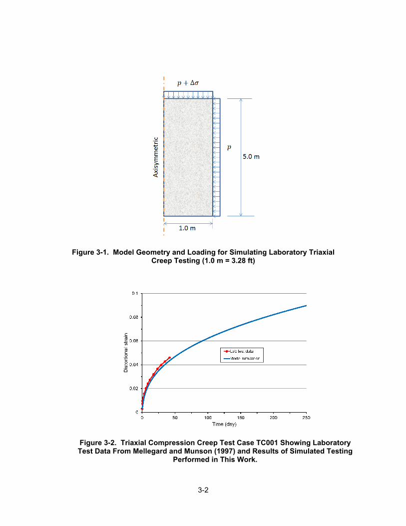
The geometrical model for the simulation consists of a cylinder specimen subjected to a confining pressure, (Figure 3-1). Then an additional axial compressive stress of magnitude ∆ was applied and held constant through the test duration. Time-dependent deformation of the specimen due to creep was calculated using FLAC with the material model described in Chapter 2. The simulation results are described in Figures 3-2 to 3-7, which compare plots of distortional strain versus time from laboratory data and model simulation, where
= 13 ( − ) = AxialStrain, = LateralStrain (3-1)
Each simulation was performed for 250 days but the laboratory tests terminated after much shorter times, except for the test shown in Figure 3-4 that also ran for 250 days. Establishing the long-term trend of the strain versus time relationship is important because the target field tests (described in Chapter 4) were run for more than 1,000 days.
The transient creep parameters , , and were evaluated by adjusting their values in the model to obtain calculated strain versus time curves that match the laboratory data from Mellegard and Munson (1997). The results are shown in Figures 3-2 through 3-7. Based on the test results (summarized in Table 3-1), we describe parameter as a function of stress ratio ⁄ (Figure 3-8), parameter as a constant value of 1250, and parameter as a function of temperature (Figure 3-9). The resulting functional definitions for and are as follows:
= + ; = 250, = 125, = ⁄ (3-2)
= + − 25+ ( − 25) = 400, = 10, = CelsiusTemperature (3-3)
3-2
Figure 3-1. Model Geometry and Loading for Simulating Laboratory Triaxial Creep Testing (1.0 m = 3.28 ft)
Figure 3-2. Triaxial Compression Creep Test Case TC001 Showing Laboratory Test Data From Mellegard and Munson (1997) and Results of Simulated Testing
Performed in This Work.

3-3
Figure 3-3. Triaxial Compression Creep Test Case TC002 Showing Laboratory Test Data From Mellegard and Munson (1997) and Results of Simulated Testing
Performed in This Work.
Figure 3-4. Triaxial Compression Creep Test Case TC003 Showing Laboratory Test Data From Mellegard and Munson (1997) and Results of Simulated Testing
Performed in This Work.

3-4
Figure 3-5. Triaxial Compression Creep Test Case TC004 Showing Laboratory Test Data From Mellegard and Munson (1997) and Results of Simulated Testing
Performed in This Work.
Figure 3-6. Triaxial Compression Creep Test Case TC006 Showing Laboratory Test Data From Mellegard and Munson (1997) and Results of Simulated Testing
Performed in This Work.
3-5
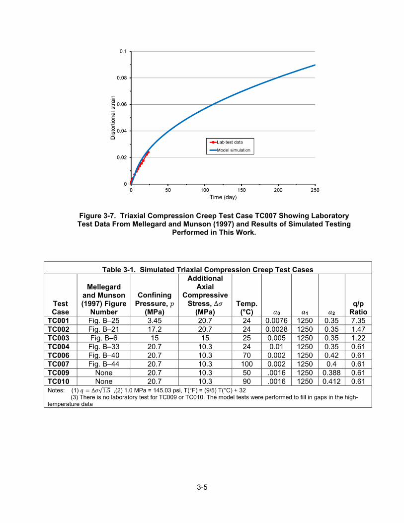
Figure 3-7. Triaxial Compression Creep Test Case TC007 Showing Laboratory Test Data From Mellegard and Munson (1997) and Results of Simulated Testing
Performed in This Work.
Table 3-1. Simulated Triaxial Compression Creep Test Cases
Test Case
Mellegard and Munson (1997) Figure
Number
Confining Pressure,
(MPa)
Additional Axial
Compressive Stress, ∆
(MPa) Temp.
(°C) 0 1 2 q/p
Ratio TC001 Fig. B–25 3.45 20.7 24 0.0076 1250 0.35 7.35 TC002 Fig. B–21 17.2 20.7 24 0.0028 1250 0.35 1.47 TC003 Fig. B–6 15 15 25 0.005 1250 0.35 1.22 TC004 Fig. B–33 20.7 10.3 24 0.01 1250 0.35 0.61 TC006 Fig. B–40 20.7 10.3 70 0.002 1250 0.42 0.61 TC007 Fig. B–44 20.7 10.3 100 0.002 1250 0.4 0.61 TC009 None 20.7 10.3 50 .0016 1250 0.388 0.61 TC010 None 20.7 10.3 90 .0016 1250 0.412 0.61 Notes: (1) = ∆ √1.5 ,(2) 1.0 MPa = 145.03 psi, T(°F) = (9/5) T(°C) + 32 (3) There is no laboratory test for TC009 or TC010. The model tests were performed to fill in gaps in the high-temperature data

3-6
Figure 3-8. Transient Creep Parameter Relationship With Stress Ratio /
Based on Results of Simulated Triaxial Compression Testing Described in This Report.
Figure 3-9. Transient Creep Parameter Relationship With Temperature Based on Results of Simulated Triaxial Compression Testing Described in This Report.
To develop the functional relationship of versus / , the value for TC004 was considered an outlier and was excluded from the relationship. Therefore, Eq. (3-2), which is represented by the blue curve in Figure 3-8, was based on the values for TC001, TC002, and TC003 in Table 3-1. The green curve in Figure 3-8 represents a rock-mass material behavior (relative to the intact rock behavior shown by the blue curve) used in the field-test model in an attempt to match the measured convergence as discussed in Chapter 4. Values of from Eq. (3-2) were used to perform additional simulated testing for test cases TC003 and TC004 because the model values for these cases differ from values based on the laboratory data. Results of the additional simulation are shown in Figure 3-10 along with the simulations for TC001 and TC002, the other
3-7
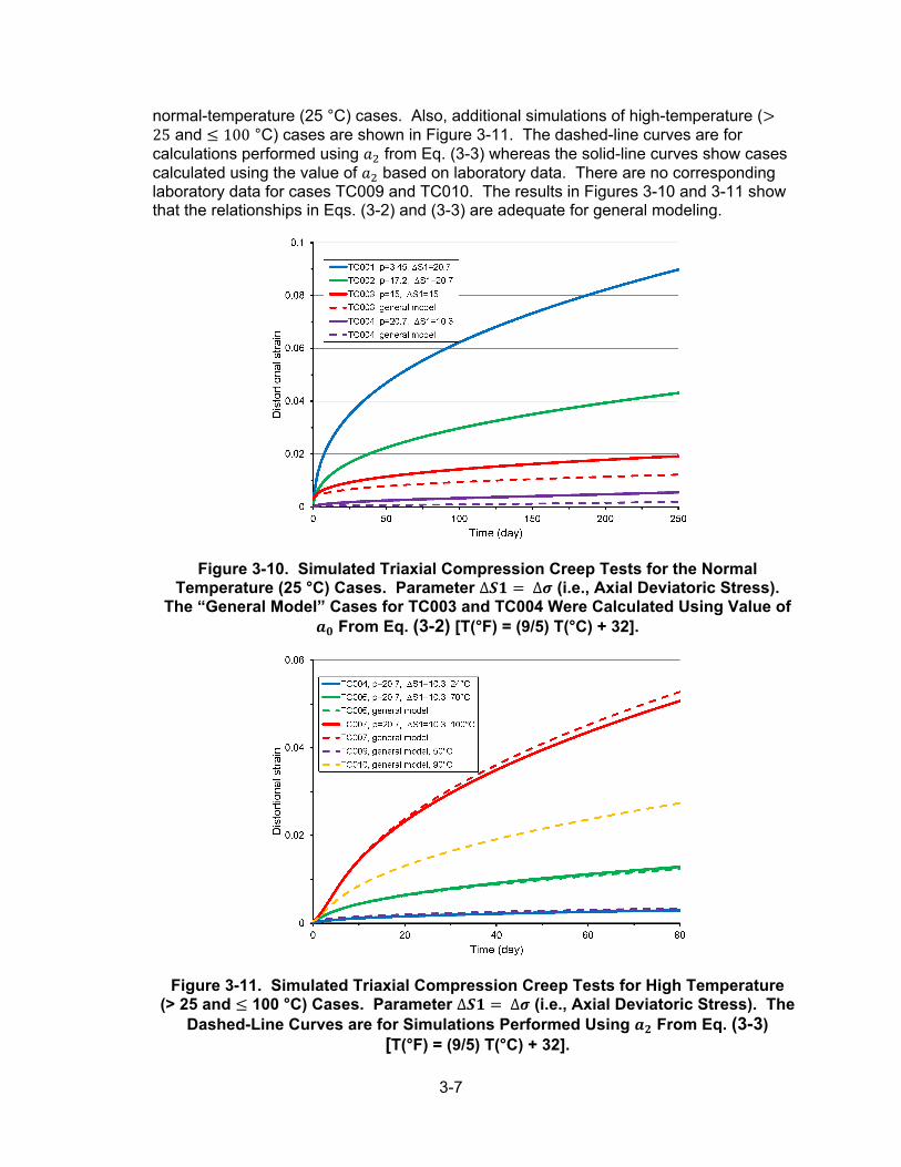
normal-temperature (25 °C) cases. Also, additional simulations of high-temperature (>25 and ≤ 100 °C) cases are shown in Figure 3-11. The dashed-line curves are for calculations performed using from Eq. (3-3) whereas the solid-line curves show cases calculated using the value of based on laboratory data. There are no corresponding laboratory data for cases TC009 and TC010. The results in Figures 3-10 and 3-11 show that the relationships in Eqs. (3-2) and (3-3) are adequate for general modeling.
Figure 3-10. Simulated Triaxial Compression Creep Tests for the Normal Temperature (25 °C) Cases. Parameter ∆ = ∆ (i.e., Axial Deviatoric Stress).
The “General Model” Cases for TC003 and TC004 Were Calculated Using Value of From Eq. (3-2) [T(°F) = (9/5) T(°C) + 32].
Figure 3-11. Simulated Triaxial Compression Creep Tests for High Temperature (> 25 and ≤ 100 °C) Cases. Parameter ∆ = ∆ (i.e., Axial Deviatoric Stress). The
Dashed-Line Curves are for Simulations Performed Using From Eq. (3-3) [T(°F) = (9/5) T(°C) + 32].

4-1
4 THERMAL AND CREEP MODELING OF WIPP ROOMS B AND D IN-SITU EXPERIMENTS
4.1 Model Description
The in-situ experiments at WIPP were simulated using FLAC with the FZK-INE salt creep model. The WIPP experiments involve measurement of long term closure of two underground test facility rooms (Rooms B and D), as described in Rath and Argüello (2012). Both rooms were constructed in bedded salt. Room D was at ambient condition while Room B was subjected to applied thermal loads using embedded heaters below the floor. The cross-sectional areas of the rooms are 5.5 m (16.4 ft) wide and 5.5 m (16.4 ft) high, located at a depth of 646 m (2118.8 ft) below the ground surface. The stratigraphy of the ground at the location of the rooms, as shown in Figure 3-1 inRath and Argüello (2012), mainly consists of argillaceous halite and halite interrupted by several horizontal clay seams. According to Rath and Argüello (2012), the “clay seams” are not distinct seams unless associated with an anhydrite layer, but are rather local horizontal concentrations of disseminated clay stringers. Rath and Argüello (2012) represented the clay seams as contact surfaces with a friction coefficient of 0.2. The clay seams were not incorporated in the current simulation.
The modeling approach is similar to that used by Rath and Argüello (2012). Site specific data and loading used in the model and the field measurement data used for comparison with model results were obtained from Rath and Argüello (2012). Two-dimensional plane strain models were developed using FLAC at the mid-section of the rooms. The test section of unheated Room D is in the middle 74.4 m (244.0 ft) of the 93.3 m (306.0 ft) long room. Room B has heaters placed below the floor along the center line of the room and symmetric about the mid-section of the room. The heaters, which simulate heat-generating radioactive waste canisters, were placed at regular intervals in bore holes in the middle 24.4 m (80.0 ft) of the 93.3 m (306.0 ft) long room. More heaters were placed at either end of the room to provide a uniform temperature distribution along the entire length of the test section. Because of these symmetries, two-dimensional models are appropriate for studying the thermal and mechanical responses of the rooms in these experiments.
The model geometry based on Rath and Argüello (2012) is shown in Figure 4-1(a). In this two-dimensional model, half of the room section was modeled using a vertical plane of symmetry along the center line of the room. The top and bottom boundary pressure is in accordance with overburden pressure (Rath and Argüello, 2012). The initial vertical stress ( ) varies linearly with depth. The horizontal stress ( ) was set to 1.5 times the vertical stress based on experimentation with the model to obtain vertical convergence greater than the horizontal convergence, as described in Section 4.2. The displacement in horizontal direction is restrained on vertical boundaries; the excavation boundary is, however, traction-free.
The thermal boundary condition is shown in Figure 4-1(b). The initial temperature of the model is 300 K [26.9 °C, 80.33 °F] and the boundaries are assumed to be at the same temperature. The heater is placed along the plane of symmetry and location and length of the heater are shown in Figure 4-2, based on Rath and Argüello (2012). The heat load, , is exponentially
decaying, as given in Eq. (4-1), where = 1.97 × 10 ( . ), =−6.331 × 10 , and ( ). = (4-1)

4-2
(a) (b) Figure 4-1. Model Geometry and Boundary Conditions for (a) Mechanical and
(b) Thermal Models (1.0 MPa = 145.03 psi, 1.0 m = 3.28 ft)
Figure 4-2. FLAC Model for Room B

4-3
The material properties for the salt used in the modelling are given in Table 4-1. The material properties in the table are for halite, which is assumed to be the representative salt for the entire model domain. The clay seams were not modeled in this analysis. The table provides the values used for density, and elastic, thermal, and creep properties. The elastic and creep properties in the table are based on the simulation of triaxial laboratory tests discussed in Section 3. Similar to Rath and Argüello (2012), the thermal conductivity, , of the salt was modeled as nonlinear function given by Eq. 4-2, where = 4.32 × 10 ( /( . . ), =1.14, and T is absolute temperature in Kelvin (K). = (300/ ) (4-2)
The modeling sequence for Room D consists of initial consolidation using initial stress conditions, simulation of excavation to develop the static stress field, and creep analysis for 1,000 days. The ambient temperature for Room D, which remained constant throughout the analysis, was assumed to be 300 K. For the heated Room B simulation, one-way coupling of thermal and mechanical response was employed. A thermal analysis was first performed using FLAC and the same model geometry to generate the temperature of the model zones for the heat load applied for a duration of 1,000 days. The computed temperature was saved at specific intervals during thermal simulation for application in the mechanical model. The mechanical model was initiated in a similar way as for the Room D model; however, creep analysis was performed for 324 days (after Rath and Argüello, 2012) at the ambient temperature of 300 K before application of the thermal load. The temperature data were fed into the mechanical model at specific times to ensure the creep and thermal times were synchronized. The zone discretization used for the models is shown in Figure 4-2.
4.2 Model Results
Results of the calculations are shown in Figures 4-3 through 4-8. The displacement contours for Room D in the vertical and horizontal directions are shown in Figure 4-3. The displacements are determined at the midpoints of the roof, floor, and sidewall, both in the field measurement and numerical calculation. Vertical closure is floor displacement minus roof displacement, and horizontal closure is right-wall displacement times -2, respecting algebraic signs. The measured convergence of Room D from the field test (Figure 4-4) shows room convergence continued to increase throughout the 1500-day test duration whereas the calculated convergence (Figure 4-5) suggests the rooms should have attained stable configurations after approximately 300 days. The difference arises because creep is the only inelastic deformation mechanism included in the model. In contrast, the measured convergence history indicates that inelastic deformation due to material failure also likely occurred during the field test.
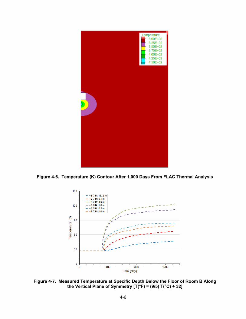
The temperature contour from FLAC thermal analysis after heating 1,000 days is shown in Figure 4-6. Compared with the measured temperatures in Figure 4-7, the calculated temperatures for Room B, shown in Figure 4-8, appear greater by about 20 °C at comparable locations and times. The difference can be attributed to greater effective heating in the two-dimensional model compared to the heating in the experiment. The results suggest the model heat load should be reduced by a small factor relative to the experimental heat load. The reduction will be considered in a subsequent calculation after implementing model changes described in Chapter 5. The thermal-mechanical analysis of Room B is ongoing and the results will be presented in future related reports with project updates.

4-4
Table 4-1. Parameters of Halite Used in the Modeling Density 2300 Kg/m3 Elastic Parameters – – Young’s Modulus 6270 MPa Poisson’s Ratio 0.45 – Thermal Parameters – – Thermal expansivity 4.2 × 10⁻⁵ 1/K
Thermal conductivity See Eq. 4-2 –
Creep Parameters – – Activation energy 54.21 kJ/mol Universal gas constant 8.31 × 10⁻³ kJ/(mol.K) Structural factor (for steady state and dilatant creep)
0.18014 MPa-5/d
Transient creep coefficients See Eq. 3-2 1/d 1750 (valid for t in days) 0.4 (valid for t in days)
Dilatant creep c-coefficients 0.75 – 750 – 0.75 –
Exponent for transient creep 5.0 – Exponent for steady state creep 5.0 – Exponent for dilatant creep – – Initial porosity of salt rock, 2.0 × 10⁻⁴ – Note: 1.0 MPa = 145.03 psi, 1.0 Kg/m3 = 0.062 lb/ft3, d = day
(a) (b) Figure 4-3. Displacement Contours for Room D After 1,000 Days: (a) Vertical
Displacement and (b) Horizontal Displacement (Displacement in m, 1 m = 3.28 ft)

4-5
Figure 4-4. Measured Vertical and Horizontal Closure Data for Room D (1 mm = 0.04 in)
Figure 4-5. Vertical and Horizontal Closure Data From FLAC Simulation Using FZK-INE Salt Model (1 mm = 0.04 in)
4-6
Figure 4-6. Temperature (K) Contour After 1,000 Days From FLAC Thermal Analysis
Figure 4-7. Measured Temperature at Specific Depth Below the Floor of Room B Along the Vertical Plane of Symmetry [T(°F) = (9/5) T(°C) + 32]

4-7
Figure 4-8. Temperature From FLAC Simulation at the Specific Depth Below the Floor of Room B Along the Vertical Line of Symmetry [T(°F) = (9/5) T(°C) + 32]

5-1
5 TECHNICAL GAPS
The calculated deformations for the WIPP Rooms B and D tests show that room convergence stabilizes after approximately 300 days (Figure 4-5); whereas, the field test data show the openings continued to converge through the test duration of approximately 1,500 days (Figure 4-4). The authors believe that the difference between the calculated response and field measurements is due to the difference between the inelastic deformation mechanism included in the model and the mechanisms active in the field test. The results suggest that inelastic deformations due to material failure and creep were active in the field test; whereas, only creep is included in the model. We modified the creep parameters to increase the rate of creep deformation in the model but the results indicate that the creep rate could not be increased enough to obtain convergence histories similar to the field measurements. In order to calculate convergence histories similar to the measurement, the model would require modifications to include deformation due to material failure in addition to creep.
As discussed in Section 2.1, the contributing deformation mechanisms in salt could include elastic, plastic, damage, thermal, and creep. The plastic and damage deformation mechanisms are related to material failure and include deformations, such as dilation and compaction. Deformation due to material failure is intrinsically time-independent but may vary with time because of time-dependency of the driving stress due to coupled creep, for example. Although the FZK-INE creep model described in Chapter 2 includes damage as a creep deformation mechanism, the damage formulation in the model is inadequate to account for potential dilation or compaction in salt. Therefore, the model described in Chapter 2 and used in the calculations described in Chapters 3 and 4 includes creep as the only inelastic deformation mechanism and needs to be modified to include deformations due to material failure.
To include deformation due to material failure, expressions will be developed for the strain increments ∆ and ∆ in Eqs. (2-1)–(2-3). The expressions can be developed through plasticity theory using a yield function that permits dilation or compaction (with associative flow rule), depending on the stress state. Such a yield function was developed for modeling clay buffer in the DECOVALEX project, as described in Manepally, et al. (2012). A similar model for salt rock will be developed using WIPP triaxial test data from Mellegard and Munson (1997) and established modeling techniques available in the literature. Following work for salt modeling is planned:
• Complete the thermal-mechanical modeling of Room B, as discussed in Chapter 4
• Develop material failure model for salt rock and crushed salt
• Application of revised model for simulation of experiments in Rooms B and D

6-1
6 REFERENCES
Desai, C.S. and H.J. Siriwardane. “Constitutive Laws for Engineering Materials with Emphasis on Geologic Materials.” Englewood Cliffs, New Jersey: Prentice-Hall, Inc. 1984.
European Commission. “Compilation of Existing Constitutive Models and Experimental Field or Laboratory Data for the Thermal-Hydraulic (THM) Modelling of the Excavation Disturbed Zone (EDZ) in Rock Salt.” Sixth Framework Programme. EURATOM Radioactive Waste Management. THERESA Project. Work Package 3 Deliverable 5. 2007.
Ghosh, A. and S. Hsiung. “Progress Report—Evaluation of Salt Under Thermomechanical Loading as a Host Repository Medium.” Center for Nuclear Waste Regulatory Analyses: San Antonio, Texas. 2013.
Itasca Consulting Group, Inc. “FLAC Fast Lagrangian Analysis of Continua.” Version 7. Minneapolis, Minnesota: Itasca Consulting Group, Inc. 2011.
Manepally, C., G. Ofoegbu, H. Basagaoglu, B. Dasgupta, and R. Fedors. “Development of a Coupled Thermohydrological-Mechanical Model.” ML12359A004. Washington, DC: U.S. Nuclear Regulatory Commission. 2012.
Mellegard, K.D. and D.E. Munson. “Laboratory Creep and Mechanical Tests on Salt Data Report (1975–1996) Waste Isolation Pilot Plant (WIPP) Thermal/Structural Interaction.” SANDIA REPORT, SAND96-2765. Albuquerque, New Mexico: Sandia National Laboratories. 1997.
Rath, J.C. and J.G. Argüello. “Revisiting Historic Numerical Analyses of the Waste Isolation Pilot Plant (WIPP) Room B and D In-Situ Experiments Regarding Thermal and Structural Response.” SANDIA REPORT, SAND2012–7525. Albuquerque, New Mexico: Sandia National Laboratories. 2012.
Winterle, J., G. Ofoegbu, R. Pabalan, C. Manepally, T. Mintz, E. Pearcy, K. Smart, J. McMurry, R. Paulin, and R. Fedors. “Geological Disposal of High-Level radioactive Waste in Salt Formations.” ML12068A057. Washington, DC: U.S. Nuclear Regulatory Commission. 2012.