implementation of conduction delay and collective ... · these schemes have been implemented on...
TRANSCRIPT
Implementation of Conduction Delay
and Collective Communication in a Parallel Spiking
Neural Network Simulator
T A H M I N A A K H T E R
Master of Science Thesis Stockholm, Sweden 2011
Implementation of Conduction Delay
and Collective Communication in a Parallel Spiking
Neural Network Simulator
T A H M I N A A K H T E R
Master’s Thesis in Biomedical Engineering (30 ECTS credits) at the Computational and Systems Biology Master Programme Royal Institute of Technology year 2011 Supervisor at CSC was Cristina Meli Examiner was Anders Lansner TRITA-CSC-E 2011:134 ISRN-KTH/CSC/E--11/134--SE ISSN-1653-5715 Royal Institute of Technology School of Computer Science and Communication KTH CSC SE-100 44 Stockholm, Sweden URL: www.kth.se/csc
Implementation of conduction delay and collective communication in a parallel spiking neural network simulator.
----------------------------------------------------------------------------------------------------------------------------- ---
Abstract As we know neural networks have a parallel structure and it is well suited for implementations in a
parallel environment. The Bayesian Confidence Propagation Neural Network (BCPNN) which has been
developed past thirty years is the main subject this thesis. An important issue is the implementation of
communications between the processors. The aim of this thesis is to investigate point to point and
collective communication methods and check how it works in real time. A second goal is to introduce
time delay in point-to-point communication. These schemes have been implemented on Blue Gene
Supercomputer using Message Passing Interface (MPI). At the end of thesis, the comparison between the
two communication methods and the results of the two different models are shown.

Implementation of conduction delay and collective communication in a parallel spiking neural network simulator.
----------------------------------------------------------------------------------------------------------------------------- ---
To my most loving father

Implementation of conduction delay and collective communication in a parallel spiking neural network simulator.
----------------------------------------------------------------------------------------------------------------------------- ---
Acknowledgements I wish to thank my supervisor and examiner Professor Anders Lansner for guiding me through the
fascinating world of computational neuroscience. I am very grateful for having the opportunity to work
with him.
I owe my co-supervisor Cristina Meli, who has always been helpful, in particular when I needed
assistance in solving the well known. A special thanks to Bernhard Kaplan who has been a great colleague
and more importantly a real good friend I ever had in Stockholm at KTH. Thank you all at the department
of Computational Biology for making our department such a pleasant place.
I would like to thank my all family members, especially my dear husband Husain Ahammad Talukdar. I
could not finish this work without his love and support.
Implementation of conduction delay and collective communication in a parallel spiking neural network simulator.
----------------------------------------------------------------------------------------------------------------------------- ---
Table of Contents
Introduction ................................................................................................................................................... 1
Chapter 1: Biological Background ................................................................................................................ 3
1.1 The Human Nervous System ............................................................................................................... 3
1.2 The Brain ............................................................................................................................................. 3
1.2.1 The Cerebral Cortex ..................................................................................................................... 4
1.2.2 Neocortex ..................................................................................................................................... 5
1.2.3 Cortical Columns .......................................................................................................................... 5
1.2.4 Hypercolumns & Minicolumns .................................................................................................... 5
1.3 Characteristics of Neurons and Synapses ............................................................................................ 6
Chapter 2: Network Structure and Methods .................................................................................................. 8
2.1 Artificial Neural Network.................................................................................................................... 8
2.1.1 Learning rule and training method ............................................................................................. 10
2.1.2 Network Architecture ................................................................................................................. 10
2.2 Detail Mathematical Neural Models ................................................................................................. 12
2.2.1 Hebbian Learning Rule............................................................................................................... 12
2.2.2 The Willshaw-Palm Model ......................................................................................................... 12
2.2.3 The Hopfield Network ................................................................................................................ 13
2.2.4 Attractor Neural Network ........................................................................................................... 14
2.2.5 The Modular Neural Networks ................................................................................................... 14
2.3 The BCPNN Model ........................................................................................................................... 15
2.3.1 Minicolumn, Hypercolumn and Connections ............................................................................. 15
2.3.2 BCPNN Learning Rule ............................................................................................................... 16
2.3.3 BCPNN with hypercolumn ......................................................................................................... 17
Chapter 3: Parallel Implementation of BCPNN .......................................................................................... 20
3.1 Parallelism in Cluster computers ....................................................................................................... 20
3.1.1 Parallel Computers ..................................................................................................................... 20
3.1.2 Distributed Memory and SPMD ................................................................................................. 21
3.1.3 Message Passing Interface (MPI) ............................................................................................... 21
3.1.4 Blue Gene / L Supercomputer .................................................................................................... 25
3.1.5 JUGENE Supercomputer............................................................................................................ 26
3.2 Implementation of BCPNN ............................................................................................................... 26
3.2.1 The Hypercolumn Module ......................................................................................................... 26
Chapter 4: Results ....................................................................................................................................... 27
4.1 Communications Comparison ........................................................................................................... 27
4.1.1 Elapsed Time .............................................................................................................................. 30

Implementation of conduction delay and collective communication in a parallel spiking neural network simulator.
----------------------------------------------------------------------------------------------------------------------------- ---
4.1.2 Run execution time (Cray Supercomputer) ................................................................................ 31
4.1.3 Count sent spikes per processor ................................................................................................. 32
4.1.4 Count sent spikes per second ...................................................................................................... 33
4.2 Point to Point Communications (with and without delay) ................................................................ 35
4.2.1 Elapsed time ............................................................................................................................... 38
4.2.2 Count sent spikes per processor ................................................................................................. 39
4.2.3 Count sent spike per second ....................................................................................................... 39
Chapter 5: Discussion .................................................................................................................................. 41
5.1 Run on Time ...................................................................................................................................... 41
5.2 Activity of sent spike ......................................................................................................................... 42
Chapter 6: Conclusion ................................................................................................................................. 43
References ................................................................................................................................................... 44
Appendix A ................................................................................................................................................. 48
A.1 Comparison communication ............................................................................................................. 48
A.2 Point to point communication (with and without delay) .................................................................. 49
Implementation of conduction delay and collective communication in a parallel spiking neural network simulator.
----------------------------------------------------------------------------------------------------------------------------- ---
The List of Figures
Figure 1: Parts of the brain [62] .................................................................................................................. 3 Figure 2: The six layer of cerebral cortex [22] ............................................................................................ 4 Figure 3 : The human cerebral cortex [38] .................................................................................................. 5 Figure 4: From neuron to neocortex[11] ...................................................................................................... 6 Figure 5: A typical nerve cell [39] ............................................................................................................... 6 Figure 6: Artificial Neural Network .............................................................................................................. 8 Figure 7: Schematic model of one ANN unit ................................................................................................. 9 Figure 8 : Mathematical model of one ANN unit. ......................................................................................... 9 Figure 9: Feedback or recurrent network ................................................................................................... 11 Figure 10 : Hopfield neural network (one layer) ........................................................................................ 13 Figure 11 : Architecture of modular neural networks [11] ........................................................................ 15 Figure 12 : Schematic architecture of hypercolumn, minicolumn and connections ................................... 16 Figure 13: BCPNN learning rules and phases ............................................................................................ 16 Figure 14: A small recurrent BCPNN with six neurons ( ) divided into three hypercolumns [13] ......... 17 Figure 15: A schematic model of a unit in a BCPNN [11] ........................................................................ 18 Figure 16: Distributed memory architecture .............................................................................................. 21 Figure 17: General MPI structure .............................................................................................................. 22 Figure 18: MPI Send/ Receive .................................................................................................................... 23 Figure 19: Point-to-point communication................................................................................................... 24 Figure 20: Collective communication (Using MPI_Allgather) ................................................................... 25 Figure 21: Flowchart of Point-to-point implementation ............................................................................. 28 Figure 22: Flowchart of Collective implementation ................................................................................... 29 Figure 23: Elapsed time of the network ...................................................................................................... 30 Figure 24: Processors elapsed time per iteration ....................................................................................... 31 Figure 25 Execution time of BG/L............................................................................................................... 31 Figure 26: Execution time of Cray ............................................................................................................. 32 Figure 27: Spike sent per network .............................................................................................................. 33 Figure 28: Bytes sent per simulated second ................................................................................................ 34 Figure 29: Bytes sent per real second ......................................................................................................... 35 Figure 30: Flowchart of time delay implementation ................................................................................... 37 Figure 31: Elapsed time of the network ...................................................................................................... 38 Figure 32: Processors elapsed time per iteration ....................................................................................... 39 Figure 33: Bytes sent per simulated second ................................................................................................ 40 Figure 34 : Bytes sent per real second ........................................................................................................ 40 Figure 35 : Compared Elapsed time (s) ...................................................................................................... 41
Implementation of conduction delay and collective communication in a parallel spiking neural network simulator.
----------------------------------------------------------------------------------------------------------------------------- ---
1
Introduction
Framework
The memory of the human brain is an incredible phenomenon. Even though day by day we are extricating
new secrets, our journey to full understanding the brain has not yet reached its goal. In the modern
science, research into the brain gathers tremendous momentum. Today neuroscience deals with a vast
number of different aspects, ranging from cognitive sciences to neurophysiology and neurocomputing.
Although the brain can work as a combined unit, neuroanatomy distinguishes different functional regions
and cerebral cortex is one of its regions.
The brain is a member of the nervous system family and controls conscious and automatic actions of all
parts of the body. The biggest part of the brain is the cerebral cortex and contains 85% weight [7]. The
cerebral cortex is a thin folded structure that covers the outer surface of the cerebral hemispheres. The
structure of the cortex appears to be homogeneous built by a number of different neuron types [10]. The
neocortex is a six-layered structure which takes up most of the cerebral cortex and is to a large extent
responsible for higher cognitive functions. It has strong internal connections which are able to adapt their
strengths. This plasticity is being modeled by different learning rules, which will be explained later. The
structure of the neocortex is manifested as a modular organization with an enormous storage capacity and
sparse activity.
One way to understand the nervous system is to use artificial neural networks (ANN). ANN has been
developed as generalizations of mathematical models of biological nervous systems. There are some
aspects that ANN has in common with neural networks, which makes them attractive to study models of
the brain: parallel processing of information, repetitive components, redundancy and adaptively. Inspired
by the ideas of Donald Hebb (1949), network models and learning rules have been developed which focus
on the learning ability of neural networks. A critique against the ANN approach mentioned e.g. presented
by Anders Lansner and Christopher Johansson (May 2004) is that (not in biological aspects) ANN are
built of non-spiking units which makes it difficult to relate the dynamics of the system to real neural
networks. As mentioned above the ability of real neurons to spike lacks in classical ANN. This
shortcoming has been overcome by the development of spiking neuron model.
The work presented here deals with neural network models of human memory based on the Bayesian
Confidence Propagating Neural Network (BCPNN). With BCPNN and many other learning rules, it has
been made possible to simulate learning mechanisms of the human nervous system.
Implementation of conduction delay and collective communication in a parallel spiking neural network simulator.
----------------------------------------------------------------------------------------------------------------------------- ---
2
Motivation
In 2006, Johansson et al. proposed “Towards cortex sized artificial neural systems” [9] and his doctoral
thesis was published (2006) “An attractor memory model of neocortex” [11]. He described the functional
model of the mammalian cortex and parallel computation employed in the brain. This thesis is partly
based on earlier work by Christopher Johansson (doctoral thesis). The aim is to find out more preciously
how the different communications work on parallel environment. The parallel implementation was done
with a Blue Gene Super computer.
From the biological point of view, real neurons communicate through synapses and generate their output
signals with a threshold function. Functional models of cortex rely on modularization and connectivity of
neurons. Only few neurons can spike at any one time and a neuron need a fair amount of synaptic input to
fire an action potential.
In particular, we exemplify the BCPNN which has a columnar structure and narrow the work in to two
goals: first, we compare the different communication requirement in cluster computer through the level of
parallelism and secondly, we introduce a time delay which investigate the amount of spike transmitted in
each processor and evaluated the scale of measurement with time step and also analyze its dynamic
performance.
In this thesis, we go from explaining the cerebral cortex of mammals, and then discuss various neural
models especially BCPNN and finish with a discussion on the implementation of this model.
Thesis Structure
The fundamental concept of human nervous system and its related parts are contained in chapter 1. There
is a description of how memories are organized and an overview of the anatomy of the nervous system.
We also present a short description of neurons and synapses.
In chapter 2, we describe the mathematical model, mainly the Hopfield neural network, the Hebbian
learning rule and other network structures. A biological interpretation of this learning rule is also
presented. The basis of BCPNN model is introduced. The environment, in which the networks can
operate, is also presented.
The focus of chapter 3 is to illustrate the parallel implementation of the BCPNN model. Firstly, there is a
review with the levels of parallel methods and short descriptions of two different supercomputers which
are today‟s fastest supercomputer. Then interest is turned on BCPNN model and how can be implemented
on the cluster computer.
In chapter 4, the two experiments are explained and we also give some significant result. The experiment
is based on execution time with model parameters done and counts the activation spike where a few basic
ideas are studied.
Chapter 5 includes further developments and the conclusion.
Finally, all experiment results raw data are listed in Appendix A.
Implementation of conduction delay and collective communication in a parallel spiking neural network simulator.
----------------------------------------------------------------------------------------------------------------------------- ---
3
Chapter 1: Biological Background In this chapter, I will introduce the fundamental facts about the human nervous system and describe the
structure of the human brain. In the following I will explain the mechanisms of neurons and synapses and
also review some knowledge about the biological subject of this thesis.
1.1 The Human Nervous System
The human nervous system is an information processing system containing a network of specialized cells
that act together to perform particular functions. The nervous system is divided into the Central Nervous
System (CNS) and the Peripheral Nervous System (PNS). The CNS is made of the brain and the spinal
cord and the PNS is made of nerves.
The human CNS contains billions of neurons. It is responsible for getting and translating signals from the
peripheral nervous system and also sends out signals to it. Brain receives sensory input from the spinal
cord and functions as primary receiver, organizer and distributor of the information about the body. The
spinal cord transmits sensory information from the PNS to the brain and motor information from the brain
to the various organs.
The PNS contains only nerve cells and connects the brain and spinal cord to the rest of the body. There are
two branches of the PNS: the somatic nervous system and the autonomic nervous system. The somatic
nervous system consists of nerve fiber that sends sensory information to the CNS and autonomic nervous
system controls many organs and muscles within the body.
1.2 The Brain
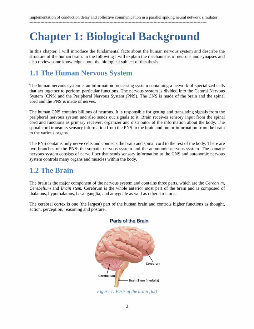
The brain is the major component of the nervous system and contains three parts, which are the Cerebrum,
Cerebellum and Brain stem. Cerebrum is the whole anterior most part of the brain and is composed of
thalamus, hypothalamus, basal ganglia, and amygdale as well as other structures.
The cerebral cortex is one (the largest) part of the human brain and controls higher functions as thought,
action, perception, reasoning and posture.
Figure 1: Parts of the brain [62]
Implementation of conduction delay and collective communication in a parallel spiking neural network simulator.
----------------------------------------------------------------------------------------------------------------------------- ---
4
1.2.1 The Cerebral Cortex
The cerebrum consists of two hemispheres, the right and left hemispheres. The two hemispheres look
mostly symmetrical yet it has been shown that each side functions slightly different than the other. Each
of these hemispheres has an outer layer which is called the cerebral cortex. The cortex covers the outer
surface of the cerebrum and cerebellum and plays a key role in versatile functionality. It is responsible for
many higher order functions such as thinking, perceiving, producing and understanding language. The
human cerebral cortex consists of approximately neurons. The cerebral cortex is divided into four
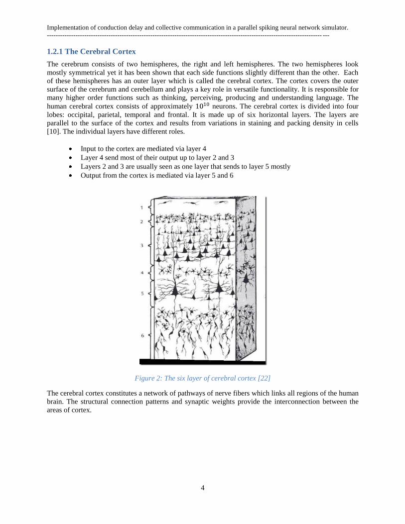
lobes: occipital, parietal, temporal and frontal. It is made up of six horizontal layers. The layers are
parallel to the surface of the cortex and results from variations in staining and packing density in cells
[10]. The individual layers have different roles.
Input to the cortex are mediated via layer 4
Layer 4 send most of their output up to layer 2 and 3
Layers 2 and 3 are usually seen as one layer that sends to layer 5 mostly
Output from the cortex is mediated via layer 5 and 6
Figure 2: The six layer of cerebral cortex [22]
The cerebral cortex constitutes a network of pathways of nerve fibers which links all regions of the human
brain. The structural connection patterns and synaptic weights provide the interconnection between the
areas of cortex.
Implementation of conduction delay and collective communication in a parallel spiking neural network simulator.
----------------------------------------------------------------------------------------------------------------------------- ---
5
1.2.2 Neocortex
Neocortex, commonly known as the phylogenetic modern cortex, is only found in mammals. It is used in
special sensory and motor processing. The evolution of neocortex is responsible for intelligence such as
performing decisions, learning and intellectual manners. In humans, 90 % of the cerebral cortex is
neocortex [66]. The neurons of the neocortex are also arranged in six horizontal layers isolated by cell
types and neuronal connections. Pyramidal and granule cell are two types of neurons that exist in all types
of cortex. The neocortex is also divided into frontal, parietal, occipital and temporal lobes. There are about
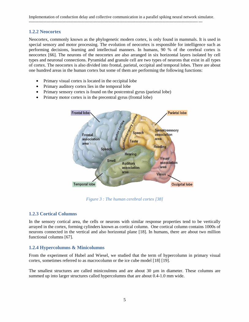
one hundred areas in the human cortex but some of them are performing the following functions:
Primary visual cortex is located in the occipital lobe
Primary auditory cortex lies in the temporal lobe
Primary sensory cortex is found on the postcentral gyrus (parietal lobe)
Primary motor cortex is in the precentral gyrus (frontal lobe)
Figure 3 : The human cerebral cortex [38]
1.2.3 Cortical Columns
In the sensory cortical area, the cells or neurons with similar response properties tend to be vertically
arrayed in the cortex, forming cylinders known as cortical column. One cortical column contains 1000s of
neurons connected in the vertical and also horizontal plane [18]. In humans, there are about two million
functional columns [67].
1.2.4 Hypercolumns & Minicolumns
From the experiment of Hubel and Wiesel, we studied that the term of hypercolumn in primary visual
cortex, sometimes referred to as macrocolumn or the ice cube model [18] [19].
The smallest structures are called minicoulmns and are about 30 µm in diameter. These columns are
summed up into larger structures called hypercolumns that are about 0.4-1.0 mm wide.
Implementation of conduction delay and collective communication in a parallel spiking neural network simulator.
----------------------------------------------------------------------------------------------------------------------------- ---
6
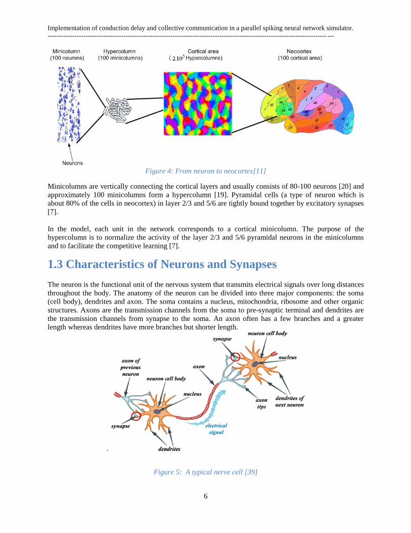
Figure 4: From neuron to neocortex[11]
Minicolumns are vertically connecting the cortical layers and usually consists of 80-100 neurons [20] and
approximately 100 minicolumns form a hypercolumn [19]. Pyramidal cells (a type of neuron which is
about 80% of the cells in neocortex) in layer 2/3 and 5/6 are tightly bound together by excitatory synapses
[7].
In the model, each unit in the network corresponds to a cortical minicolumn. The purpose of the
hypercolumn is to normalize the activity of the layer 2/3 and 5/6 pyramidal neurons in the minicolumns
and to facilitate the competitive learning [7].
1.3 Characteristics of Neurons and Synapses
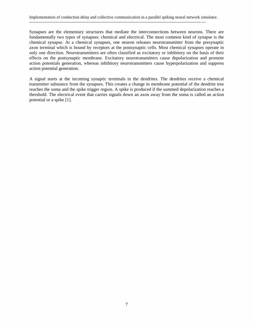
The neuron is the functional unit of the nervous system that transmits electrical signals over long distances
throughout the body. The anatomy of the neuron can be divided into three major components: the soma
(cell body), dendrites and axon. The soma contains a nucleus, mitochondria, ribosome and other organic
structures. Axons are the transmission channels from the soma to pre-synaptic terminal and dendrites are
the transmission channels from synapse to the soma. An axon often has a few branches and a greater
length whereas dendrites have more branches but shorter length.
.
Figure 5: A typical nerve cell [39]
Implementation of conduction delay and collective communication in a parallel spiking neural network simulator.
----------------------------------------------------------------------------------------------------------------------------- ---
7
Synapses are the elementary structures that mediate the interconnections between neurons. There are
fundamentally two types of synapses: chemical and electrical. The most common kind of synapse is the
chemical synapse. At a chemical synapses, one neuron releases neurotransmitter from the presynaptic
axon terminal which is bound by receptors at the postsynaptic cells. Most chemical synapses operate in
only one direction. Neurotransmitters are often classified as excitatory or inhibitory on the basis of their
effects on the postsynaptic membrane. Excitatory neurotransmitters cause depolarization and promote
action potentials generation, whereas inhibitory neurotransmitters cause hyperpolarization and suppress
action potential generation.
A signal starts at the incoming synaptic terminals in the dendrites. The dendrites receive a chemical
transmitter substance from the synapses. This creates a change in membrane potential of the dendrite tree
reaches the soma and the spike trigger region. A spike is produced if the summed depolarization reaches a
threshold. The electrical event that carries signals down an axon away from the soma is called an action
potential or a spike [1].
Implementation of conduction delay and collective communication in a parallel spiking neural network simulator.
----------------------------------------------------------------------------------------------------------------------------- ---
8
Chapter 2: Network Structure and
Methods Within the field of Artificial Neural Network (ANN), there are a huge number of different network
structures and various learning algorithms. Here I focus on a few types of network structure with their
context and definitions. First I explain how a basic ANN is built. I give its mathematical formulation and
discuss its specific features and how they account for biologically observed phenomena. Finally, the
BCPNN model is described.
2.1 Artificial Neural Network
Commonly, artificial neural networks (ANN‟s) are referred to as neural networks. ANN is an
interconnected group of nodes, where nodes are called neurons or processing elements or units. An ANN
is a computational model inspired by the natural brain. The important components of neural networks are
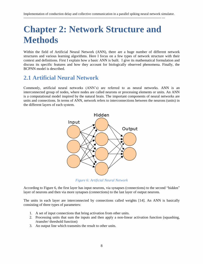
units and connections. In terms of ANN, network refers to interconnections between the neurons (units) in
the different layers of each system.
Figure 6: Artificial Neural Network
According to Figure 6, the first layer has input neurons, via synapses (connections) to the second “hidden”
layer of neurons and then via more synapses (connections) to the last layer of output neurons.
The units in each layer are interconnected by connections called weights [14]. An ANN is basically
consisting of three types of parameters:
1. A set of input connections that bring activation from other units.
2. Processing units that sum the inputs and then apply a non-linear activation function (squashing,
/transfer/ threshold function)
3. An output line which transmits the result to other units.
Implementation of conduction delay and collective communication in a parallel spiking neural network simulator.
----------------------------------------------------------------------------------------------------------------------------- ---
9
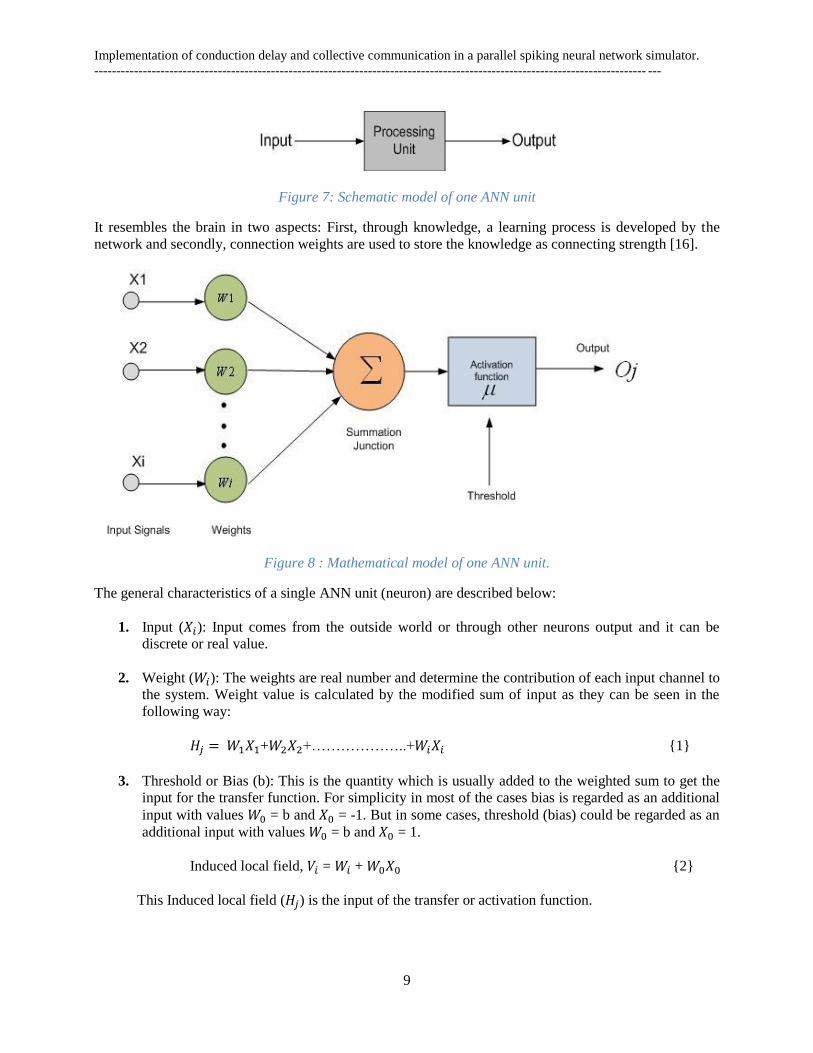
Figure 7: Schematic model of one ANN unit
It resembles the brain in two aspects: First, through knowledge, a learning process is developed by the
network and secondly, connection weights are used to store the knowledge as connecting strength [16].
Figure 8 : Mathematical model of one ANN unit.
The general characteristics of a single ANN unit (neuron) are described below:
1. Input ( ): Input comes from the outside world or through other neurons output and it can be
discrete or real value.
2. Weight ( ): The weights are real number and determine the contribution of each input channel to
the system. Weight value is calculated by the modified sum of input as they can be seen in the
following way:
+ +………………..+ {1}
3. Threshold or Bias (b): This is the quantity which is usually added to the weighted sum to get the
input for the transfer function. For simplicity in most of the cases bias is regarded as an additional
input with values = b and = -1. But in some cases, threshold (bias) could be regarded as an
additional input with values = b and = 1.
Induced local field, = + {2}
This Induced local field ( ) is the input of the transfer or activation function.
Implementation of conduction delay and collective communication in a parallel spiking neural network simulator.
----------------------------------------------------------------------------------------------------------------------------- ---
10
4. Transfer/Activity function: The transfer function is the function giving the input-output behavior
of an artificial neural network for one unit. Several functions can be used for describing the
transfer function: Step function (Threshold function), linear function, Gaussian, Identity and
sigmoid function [27]. Most of them are non-linear and has limited output range.
5. Output ( ): Each unit computes the output from the weighted input values through a non-linear
activation function. The equation is defined as [27]:
= {3}
Depending on the type of activation function, a neuron can produce different type of output value. For
example, when the activation function is a step function, the output is 1 if the sum of the inputs is above a
threshold, otherwise it is 0.
Most ANN models are not a very good or accurate description of biological network, but should rather be
seen as biological inspired algorithms. The Learning rule and the network architecture are two important
aspects of artificial neural model.
2.1.1 Learning rule and training method
The learning rule is an algorithm that modifies connections between units. Learning implies that a
processing unit is capable of changing its input/ output behavior as a result of changes in the environment.
Weights are used for considering a suitable learning rule and training method.
In the training phase, the correct output for each record is known, and the output nodes can be assigned „1‟
for correct values and „0‟ for others. It is thus possible to compare the network‟s output with these correct
values and find the error term for each node. During the learning phase, the network learns by adjusting
the weights to be able to predict the correct output from input samples, refers to the learning rule in eq.
(1).
Various methods to set the strength of connections exist. One way is to set the weights explicitly, using a
priori knowledge. Another way is to train the neural network by feeding it with training pattern and
letting it changes the weights according to some learning rule. In some sense, it can adjust all the
necessary weights but this might be complicated for many networks. The more conventional learning
process in artificial neural networks can be divided into supervised, reinforcement and unsupervised
learning methods. Supervised learning is a learning process based on comparison between networks
computed output and the correct expected output, generating error. In unsupervised learning, an output
unit is trained to respond to cluster of pattern within the input. The following section (2.2.3), Hopfield
models use the unsupervised training algorithm for the update of weights.
2.1.2 Network Architecture
Network architecture can have several topologies, but particularly we can differentiate it by the layer
structures and direction of communication. Connections between units in the network can be sparse or all-
to-all. As for this pattern connection, artificial neural model is divided by the: feed-forward network
(single and multi-layer network) and feed-back network (recurrent network).
Implementation of conduction delay and collective communication in a parallel spiking neural network simulator.
----------------------------------------------------------------------------------------------------------------------------- ---
11
Feed-forward network:
In feed-forward network, the connections between units contain no directed cycles. There is no feedback
between layers. The connections imply that the neuron in each layer of the network have as their only
input the activation output of the neurons of the previous layer. This process continues until it has gone
through all layers and determines the output. They can be including one or more hidden layers. Perception
learning and Delta rule learning is a classical learning rule of feed-forward network and often used as data
mining.
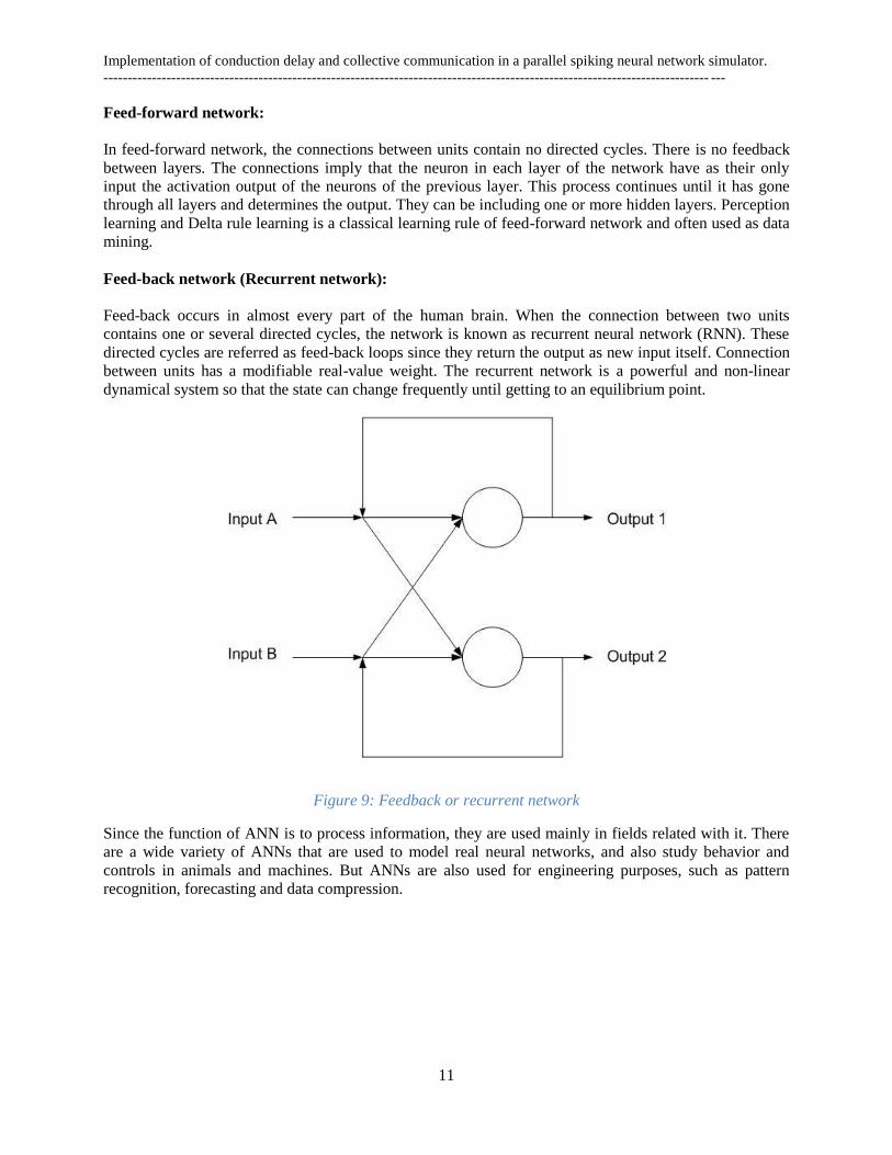
Feed-back network (Recurrent network):
Feed-back occurs in almost every part of the human brain. When the connection between two units
contains one or several directed cycles, the network is known as recurrent neural network (RNN). These
directed cycles are referred as feed-back loops since they return the output as new input itself. Connection
between units has a modifiable real-value weight. The recurrent network is a powerful and non-linear
dynamical system so that the state can change frequently until getting to an equilibrium point.
Figure 9: Feedback or recurrent network
Since the function of ANN is to process information, they are used mainly in fields related with it. There
are a wide variety of ANNs that are used to model real neural networks, and also study behavior and
controls in animals and machines. But ANNs are also used for engineering purposes, such as pattern
recognition, forecasting and data compression.
Implementation of conduction delay and collective communication in a parallel spiking neural network simulator.
----------------------------------------------------------------------------------------------------------------------------- ---
12
2.2 Detail Mathematical Neural Models
Here, we discuss several approaches for creating memory in a neural network context and also give its
mathematical formulation and explain their learning method.
2.2.1 Hebbian Learning Rule
The learning paradigms discussed above result in an adjustment of the weights of the connections between
units, according to some modification rule. Perhaps the most influential work in connectionism‟s history is
the contribution of Hebb (1949), where he presented a theory of behavior based, as much possible on the
physiology of the nervous system [23].
The most important concept emerged from Hebb‟s work was his formal statement (known as Hebb‟s
postulate) of how learning could occur. Hebb‟s original statement summarize about “Cell connectivity
strength changes” or “cells that fire together, wire together”. From the theory:
when an axon of cell A is near enough excite a cell B and repeatedly or persistently takes part in firing it,
some growth process or metabolic change takes place in one or both cells such that A’s efficiency as one
of the cells firing B, is increased.[23]
The basic idea is that the weights of the connections between two units should be increased or decreased
according to their activation [23]. In Hebb‟s theory, if two neurons are active simultaneously, their
interactions must be strengthened. Hebbian cell assemblies can be represented in recurrent or all-to-all
fashion [24]. The Hebbian rule works well as long as all the input patterns are orthogonal or uncorrelated
[64]. In this thesis, the main concern is the attractor network theories of cortical associative memory.
If and are the activation of neurons, is the connection weight matrix and γ is the learning rate
parameter, then Hebb‟s rule has been written as modifying pattern of connectivity:
∆ = γ ; Where ∆ is the change of component ij of the connection weight matrix. [26]
This form of learning is called Hebbian learning rule.
2.2.2 The Willshaw-Palm Model
Associative memory is a system which stores mapping from specific input representations to specific
output representations. It consists of feed-forward connections. We have derived the Willshaw-Palm
model by owing from the two different investigators. The associative network from the Willshaw model
[30] analyzed the input-output patterns of a two layers feed-forward network with binary activity and the
Palm model [31] is applied one-layer feed-forward network for training interactively according to
reinforcement learning with binary synaptic weights. The binary output pattern can be defined by
and non-linear threshold function [11]. In the training procedure, each pair of the mapping is
presented to the network. The learning rule is described for generating the weight matrix, where
:
Q is the total number of patterns.
Implementation of conduction delay and collective communication in a parallel spiking neural network simulator.
----------------------------------------------------------------------------------------------------------------------------- ---
13
2.2.3 The Hopfield Network
The idea behind the Hopfield network is largely based on Donald Hebb‟s well known work: assume that
we have a set of neurons, which are connected to each other through connection-weights [28]. In discrete
Hopfield neural network (HNN), the neurons can either be active or non-active and there exist parallel
input and output channels. The Hopfield model is a single layer processing unit and its input pattern is
binary and activation function can be sigmoid or hard limiter. This means that the output of a Hopfield
model is depending whether the input is less than or greater than the threshold value [28]. The HNN is the
most implemented associative memory network and serves as content addressable memory (CAM) with
binary threshold units.
If the network is trained with a pattern and then fed with a partial pattern that fits the learned pattern, it
will stimulate the remaining neurons of the pattern to become active, completing it. If two neurons are
anti-correlated (one neuron is active while the other neuron is not) the connection-weights between them
are weakened or become inhibitory.
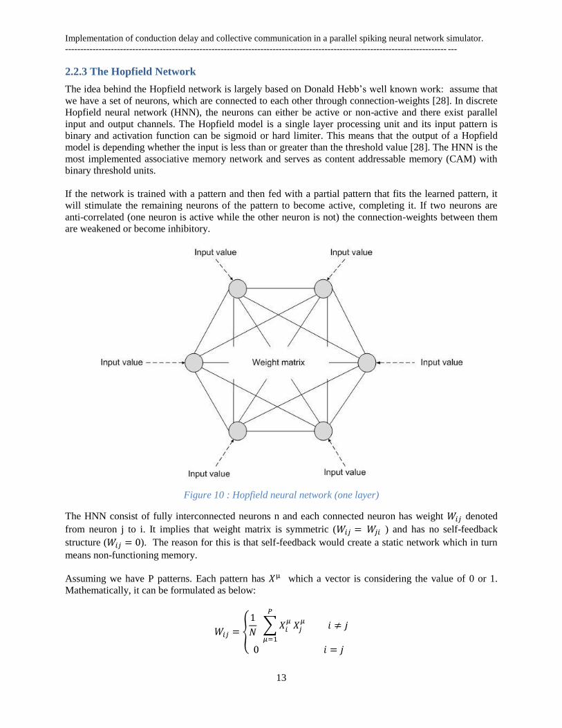
Figure 10 : Hopfield neural network (one layer)
The HNN consist of fully interconnected neurons n and each connected neuron has weight denoted
from neuron j to i. It implies that weight matrix is symmetric ( ) and has no self-feedback
structure ( ). The reason for this is that self-feedback would create a static network which in turn
means non-functioning memory.
Assuming we have P patterns. Each pattern has which a vector is considering the value of 0 or 1.
Mathematically, it can be formulated as below:
Implementation of conduction delay and collective communication in a parallel spiking neural network simulator.
----------------------------------------------------------------------------------------------------------------------------- ---
14
Where,
P is the number of training patterns.
μ is the index within the set of training patterns.
N is the number of units (neurons) in a pattern.
The patterns represent activation of the neurons and neurons can be in the states ⋲ {+1, - 1}. To recall
an output pattern (of activation), in this network we can use an arbitrary neuron i and the update rule
can be specified by:
(If hard limiter active functions)
Each network has energy in quadratic form. The energy function can be defined as:
Where denotes the value of at each iteration.
The (Lyapunov) energy function [65] is a monotonically decreasing function of time [29]. The maximum
storage capacity with error on recall of the Hopfield network is about 0.14N patterns [29]. The successive
updating of the state in the network is a convergence process and as a result the energy of the system gets
minimized [28]. The asynchronous updating rule from its initial state will allow a minimum energy state
to be achieved. In Hopfield network model, oscillation may occur. The model also has problem with
catastrophic forgetting (If the network is loaded with many pattern and will not be able to recall any
pattern at all).
2.2.4 Attractor Neural Network
An attractor network in its simplest form is an artificial neural network comprised of units connected in a
recurrent, all-to-all fashion. Clarifying the involved terms such as dynamical system is just an
interconnected network of neurons and describing how the state of neurons and synapses evolve in time. If
the connection matrix is symmetric, the dynamics is particularly simple. The computation starts in some
initial input state, then follows a trajectory in state space and may finally converge to a stable output state
(attractor). Energy function can define over the states of the network. If the connectivity is asymmetric,
more complex dynamics in the form of limit cycles and disorder activity may result [24].
2.2.5 The Modular Neural Networks
The inspiration for modular design of neural networks is mainly due to biological reasons. The modularity
is a key to the efficient and intelligent working of human brain. Vertebrate nervous systems operate on
the principle of modularity and the nervous system is comprised of different modules dedicated to
different subtasks working together to accomplish a complex task [32]. The modular behavior of the brain
is of two types: Structural modularity and Functional modularity. Structural modularity is evident from
sparse connections between strongly connected neuronal groups. Functional modularity is indicated by the
fact that neural modules have different neural response patterns which are grouped together.
Implementation of conduction delay and collective communication in a parallel spiking neural network simulator.
----------------------------------------------------------------------------------------------------------------------------- ---
15
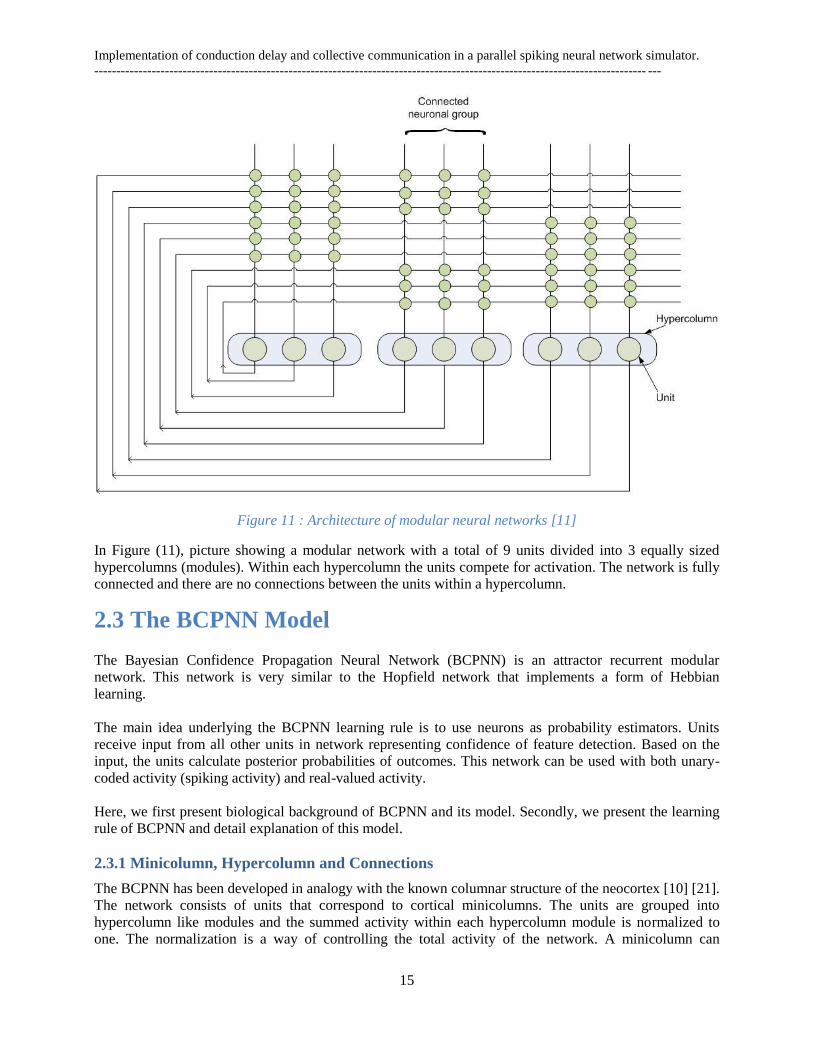
Figure 11 : Architecture of modular neural networks [11]
In Figure (11), picture showing a modular network with a total of 9 units divided into 3 equally sized
hypercolumns (modules). Within each hypercolumn the units compete for activation. The network is fully
connected and there are no connections between the units within a hypercolumn.
2.3 The BCPNN Model
The Bayesian Confidence Propagation Neural Network (BCPNN) is an attractor recurrent modular
network. This network is very similar to the Hopfield network that implements a form of Hebbian
learning.
The main idea underlying the BCPNN learning rule is to use neurons as probability estimators. Units
receive input from all other units in network representing confidence of feature detection. Based on the
input, the units calculate posterior probabilities of outcomes. This network can be used with both unary-
coded activity (spiking activity) and real-valued activity.
Here, we first present biological background of BCPNN and its model. Secondly, we present the learning
rule of BCPNN and detail explanation of this model.
2.3.1 Minicolumn, Hypercolumn and Connections
The BCPNN has been developed in analogy with the known columnar structure of the neocortex [10] [21].
The network consists of units that correspond to cortical minicolumns. The units are grouped into
hypercolumn like modules and the summed activity within each hypercolumn module is normalized to
one. The normalization is a way of controlling the total activity of the network. A minicolumn can
Implementation of conduction delay and collective communication in a parallel spiking neural network simulator.
----------------------------------------------------------------------------------------------------------------------------- ---
16
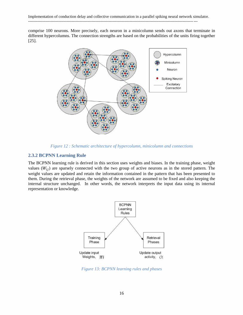
comprise 100 neurons. More precisely, each neuron in a minicolumn sends out axons that terminate in
different hypercolumns. The connection strengths are based on the probabilities of the units firing together
[25].
Figure 12 : Schematic architecture of hypercolumn, minicolumn and connections
2.3.2 BCPNN Learning Rule
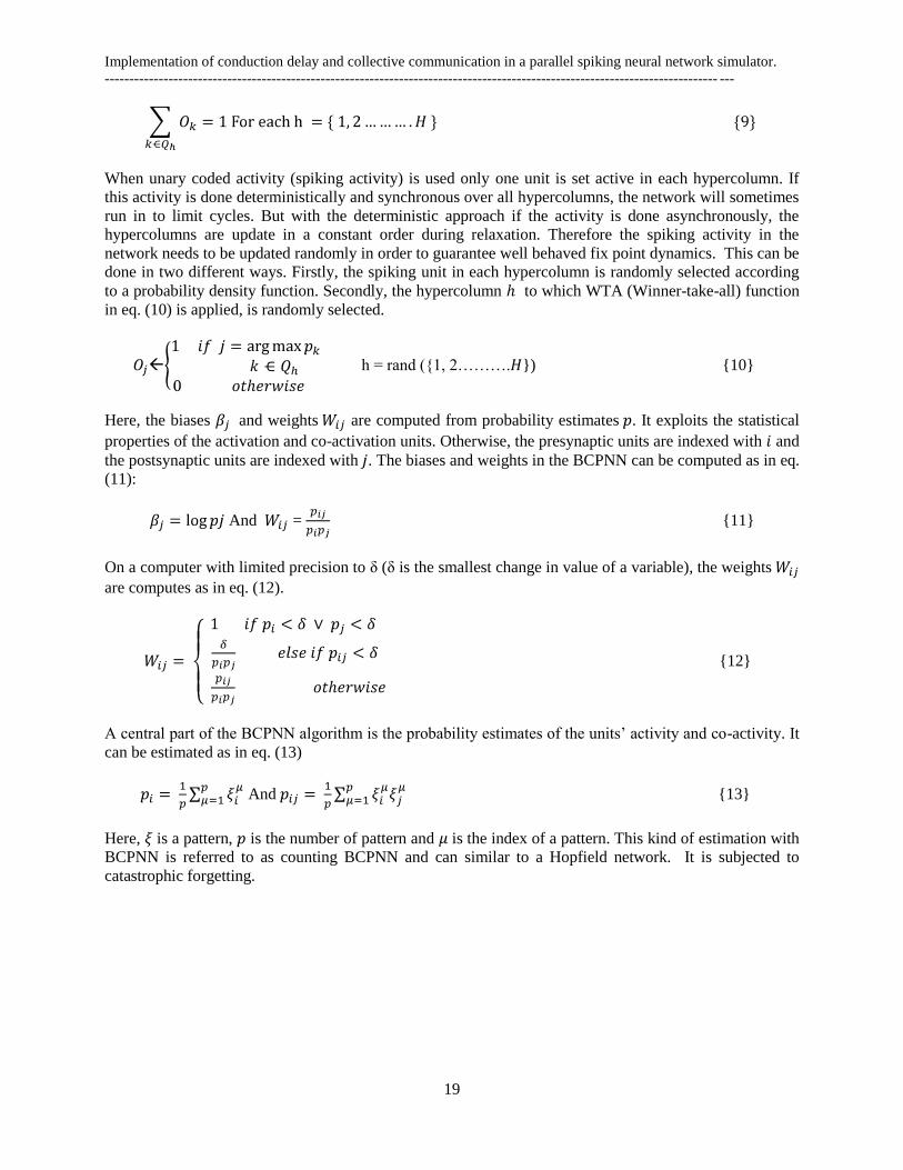
The BCPNN learning rule is derived in this section uses weights and biases. In the training phase, weight
values ( ) are sparsely connected with the two group of active neurons as in the stored pattern. The
weight values are updated and retain the information contained in the pattern that has been presented to
them. During the retrieval phase, the weights of the network are assumed to be fixed and also keeping the
internal structure unchanged. In other words, the network interprets the input data using its internal
representation or knowledge.
Figure 13: BCPNN learning rules and phases
Implementation of conduction delay and collective communication in a parallel spiking neural network simulator.
----------------------------------------------------------------------------------------------------------------------------- ---
17
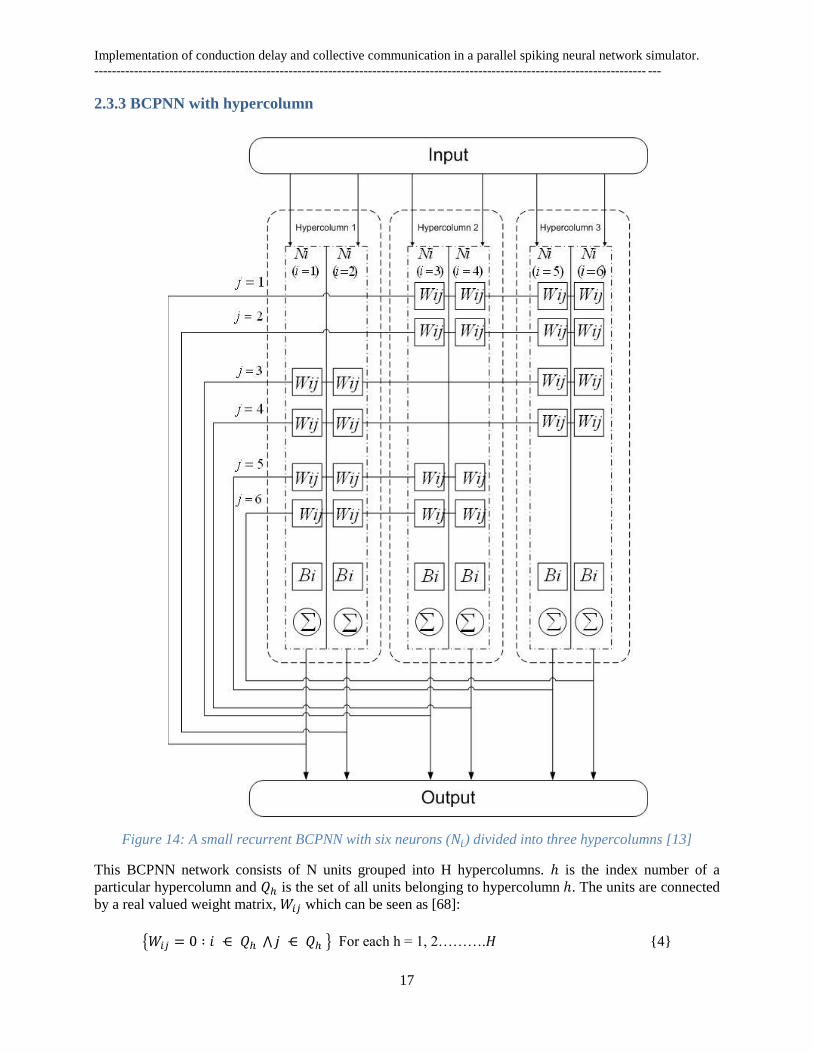
2.3.3 BCPNN with hypercolumn
Figure 14: A small recurrent BCPNN with six neurons ( ) divided into three hypercolumns [13]
This BCPNN network consists of N units grouped into H hypercolumns. is the index number of a
particular hypercolumn and is the set of all units belonging to hypercolumn . The units are connected
by a real valued weight matrix, which can be seen as [68]:
For each h = 1, 2………. {4}
Implementation of conduction delay and collective communication in a parallel spiking neural network simulator.
----------------------------------------------------------------------------------------------------------------------------- ---
18
It is noted that there are no connections within a hypercolumn.
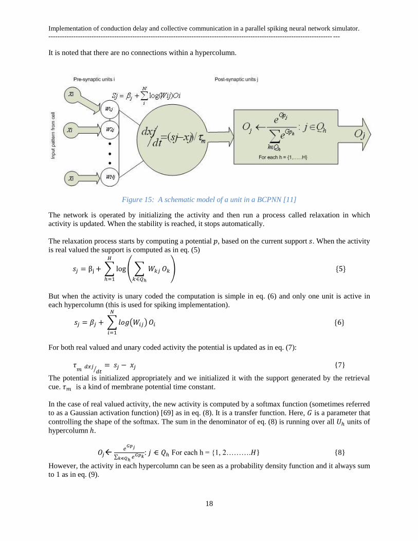
Figure 15: A schematic model of a unit in a BCPNN [11]
The network is operated by initializing the activity and then run a process called relaxation in which
activity is updated. When the stability is reached, it stops automatically.
The relaxation process starts by computing a potential , based on the current support . When the activity
is real valued the support is computed as in eq. (5)
But when the activity is unary coded the computation is simple in eq. (6) and only one unit is active in
each hypercolumn (this is used for spiking implementation).
For both real valued and unary coded activity the potential is updated as in eq. (7):
{7}
The potential is initialized appropriately and we initialized it with the support generated by the retrieval
cue. is a kind of membrane potential time constant.
In the case of real valued activity, the new activity is computed by a softmax function (sometimes referred
to as a Gaussian activation function) [69] as in eq. (8). It is a transfer function. Here, is a parameter that
controlling the shape of the softmax. The sum in the denominator of eq. (8) is running over all units of
hypercolumn .
: For each h = {1, 2………. } {8}
However, the activity in each hypercolumn can be seen as a probability density function and it always sum
to 1 as in eq. (9).
Implementation of conduction delay and collective communication in a parallel spiking neural network simulator.
----------------------------------------------------------------------------------------------------------------------------- ---
19
When unary coded activity (spiking activity) is used only one unit is set active in each hypercolumn. If
this activity is done deterministically and synchronous over all hypercolumns, the network will sometimes
run in to limit cycles. But with the deterministic approach if the activity is done asynchronously, the
hypercolumns are update in a constant order during relaxation. Therefore the spiking activity in the
network needs to be updated randomly in order to guarantee well behaved fix point dynamics. This can be
done in two different ways. Firstly, the spiking unit in each hypercolumn is randomly selected according
to a probability density function. Secondly, the hypercolumn to which WTA (Winner-take-all) function
in eq. (10) is applied, is randomly selected.
h = rand ({1, 2………. }) {10}
Here, the biases and weights are computed from probability estimates . It exploits the statistical
properties of the activation and co-activation units. Otherwise, the presynaptic units are indexed with and
the postsynaptic units are indexed with . The biases and weights in the BCPNN can be computed as in eq.
(11):
And = {11}
On a computer with limited precision to δ (δ is the smallest change in value of a variable), the weights
are computes as in eq. (12).
{12}
A central part of the BCPNN algorithm is the probability estimates of the units‟ activity and co-activity. It
can be estimated as in eq. (13)
And {13}
Here, is a pattern, is the number of pattern and is the index of a pattern. This kind of estimation with
BCPNN is referred to as counting BCPNN and can similar to a Hopfield network. It is subjected to
catastrophic forgetting.
Implementation of conduction delay and collective communication in a parallel spiking neural network simulator.
----------------------------------------------------------------------------------------------------------------------------- ---
20
Chapter 3: Parallel Implementation of
BCPNN In this chapter, we introduce how the BCPNN can be implemented in a parallel environment. Internal
computation of the BCPNN network requires a great amount of processor time. To be able to simulate
large networks, a cluster of computers is required rather than serial environment. This is the reason why
one of the world fastest supercomputer Blue Gene/L is used.
In order to have a matching from the BCPNN model, I will emphasize the basic idea about the parallel
techniques and also discuss its specific features and how they account for cluster computers.
Mapping as, 1 Hypercolumn = 1 Processor (contain 100 processing units)
3.1 Parallelism in Cluster computers
The mammalian brain is a very powerful and flexible computing system. In the thesis, I am discussing the
efficient implementations of BCPNN with parallel computations. In a cluster computer, the designer
should be able to improve performance proportionally with added processors. The computer clusters are
usually constructed to provide optimal communication between processors. The approach of parallel
computation in cortical model will allow not only operating larger network models faster than before but
also it will show the naturalistic behavior of neocortex.
When considering a model of the cortex it is important that it scales well in terms of implementation. Two
main properties of the parallel computation are strong scaling and weak scaling. Strong scaling means that
we fix the problem size, vary the number of processors and measure the speedup. Weak scaling means we
vary the problem size and the number of processors such that the execution time is the same.
ANNs that use non-local computations typically have weak scaling properties; it is costly in
communication [9]. More biologically realistic models implement learning rules that only require local
computations such as Hebbian learning rule, attractor network [51]. The advantage of local learning rules
is that they have a potential to scale well.
3.1.1 Parallel Computers
Traditionally, programs have been written in serial environment. But for large calculations and faster
executions, parallel environment is a must. The reasons for using parallel computer are not only for saving
time but also to solve large problems. The classification of parallel computer can be divided into SIMD
(Single Instruction, Multiple Data) and MIMD (Multiple Instruction, Multiple Data). Memory distribution
of parallel computer is classified by shared memory and distributed memory.
In shared memory, multiple processors can operate independently by sharing the same memory space and
in distributed memory, multiple processors can operate their own local memory space but require a
communication network to connect between inter processors memory. Message Passing Interface (MPI) is
a library with portable standard programming language for parallel computers and it is effectively used for
message communication. Usually, MPI is well suited for computing distributed memory but it can also be
applied into shared memory architecture.
Implementation of conduction delay and collective communication in a parallel spiking neural network simulator.
----------------------------------------------------------------------------------------------------------------------------- ---
21
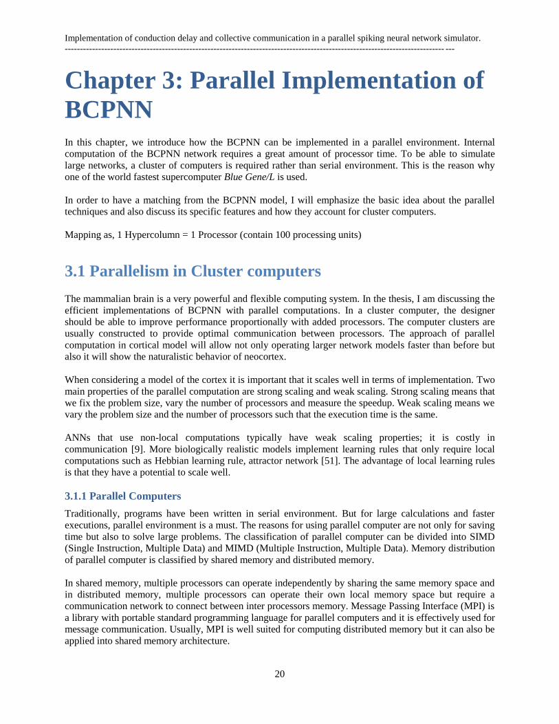
3.1.2 Distributed Memory and SPMD
In distributed memory system, there is usually a CPU, a memory and some form of interconnection
network that provides programs on each processor to interconnect each other. Each CPU can utilize the
full bandwidth to its local memory without interference from other CPUs. Data is shared across a
communication network and responsible for synchronization using message passing.
Figure 16: Distributed memory architecture
Single Program Multiple Data (SPMD) is a parallel technique which develops multiple data against a
single program to perform operations. The implementation of SPMD requires that commonly available
functionality in the serial environment be provided in the parallel environment in such a way that the serial
source code can be used on the distributed memory machine. With SPMD, tasks can be executed on
general purpose CPUs but SIMD is suitable for vector processors.
3.1.3 Message Passing Interface (MPI)
MPI is a message passing library that was developed in the early 90s [36]. It allows processes to
communicate with one another by sending and receiving messages. The programming model of MPI is
commonly used in SPMD mode. It should be noted that the basic feature of MPI implementation offers its
own parallel programming environment. Typically, MPI is used as a communication protocol for cluster
computers and supercomputers. The target platform is a distributed memory system such as single
program. MPI offers standardization, portability, performance opportunities, functionality and availability
[42].
Implementation of conduction delay and collective communication in a parallel spiking neural network simulator.
----------------------------------------------------------------------------------------------------------------------------- ---
22
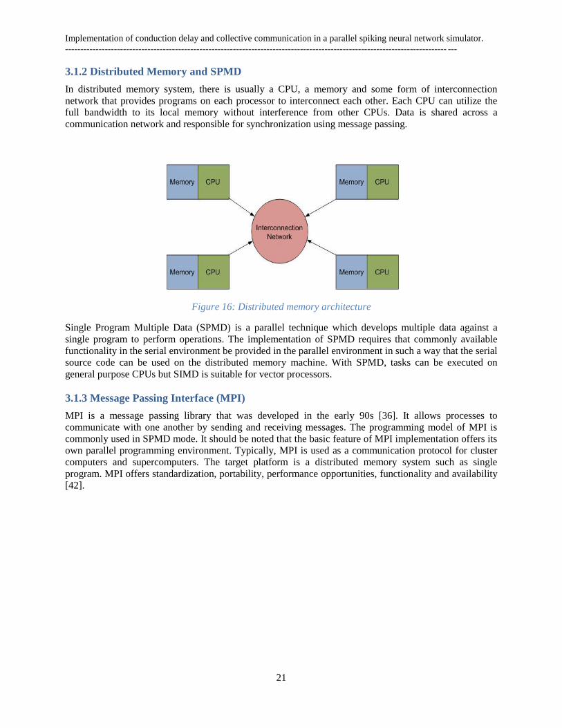
Figure 17: General MPI structure
MPI provide a rich range of capabilities and always work with processes but commonly refers to
processes or processors. Processes have unique ranks associated with communicator, number from 0 to n-
1 [43]. The following concepts help in understanding and providing the context of that functionality:
I. MPI Basic Send/Receive
II. Point-to-point Communication
III. Collective Communication
I. MPI Basic Send / Receive:
Message passing is an approach that makes the exchange of data cooperative and data must both be
explicitly sent and received. The message passing model is defined as:
Set of processes using only local memory
Processes communicate by sending and receiving messages
Data transfer requires cooperative operations to be performed by each process.
Implementation of conduction delay and collective communication in a parallel spiking neural network simulator.
----------------------------------------------------------------------------------------------------------------------------- ---
23
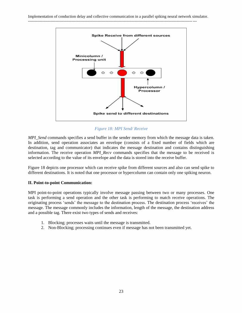
Figure 18: MPI Send/ Receive
MPI_Send commands specifies a send buffer in the sender memory from which the message data is taken.
In addition, send operation associates an envelope (consists of a fixed number of fields which are
destination, tag and communicator) that indicates the message destination and contains distinguishing
information. The receive operation MPI_Recv commands specifies that the message to be received is
selected according to the value of its envelope and the data is stored into the receive buffer.
Figure 18 depicts one processor which can receive spike from different sources and also can send spike to
different destinations. It is noted that one processor or hypercolumn can contain only one spiking neuron.
II. Point-to-point Communication:
MPI point-to-point operations typically involve message passing between two or many processes. One
task is performing a send operation and the other task is performing to match receive operations. The
originating process „sends‟ the message to the destination process. The destination process „receives‟ the
message. The message commonly includes the information, length of the message, the destination address
and a possible tag. There exist two types of sends and receives:
1. Blocking; processes waits until the message is transmitted.
2. Non-Blocking; processing continues even if message has not been transmitted yet.
Implementation of conduction delay and collective communication in a parallel spiking neural network simulator.
----------------------------------------------------------------------------------------------------------------------------- ---
24
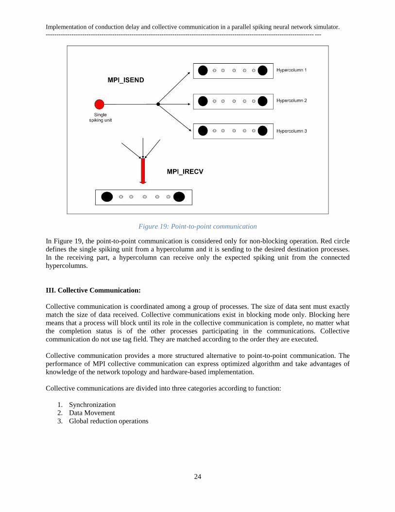
Figure 19: Point-to-point communication
In Figure 19, the point-to-point communication is considered only for non-blocking operation. Red circle
defines the single spiking unit from a hypercolumn and it is sending to the desired destination processes.
In the receiving part, a hypercolumn can receive only the expected spiking unit from the connected
hypercolumns.
III. Collective Communication:
Collective communication is coordinated among a group of processes. The size of data sent must exactly
match the size of data received. Collective communications exist in blocking mode only. Blocking here
means that a process will block until its role in the collective communication is complete, no matter what
the completion status is of the other processes participating in the communications. Collective
communication do not use tag field. They are matched according to the order they are executed.
Collective communication provides a more structured alternative to point-to-point communication. The
performance of MPI collective communication can express optimized algorithm and take advantages of
knowledge of the network topology and hardware-based implementation.
Collective communications are divided into three categories according to function:
1. Synchronization
2. Data Movement
3. Global reduction operations
Implementation of conduction delay and collective communication in a parallel spiking neural network simulator.
----------------------------------------------------------------------------------------------------------------------------- ---
25
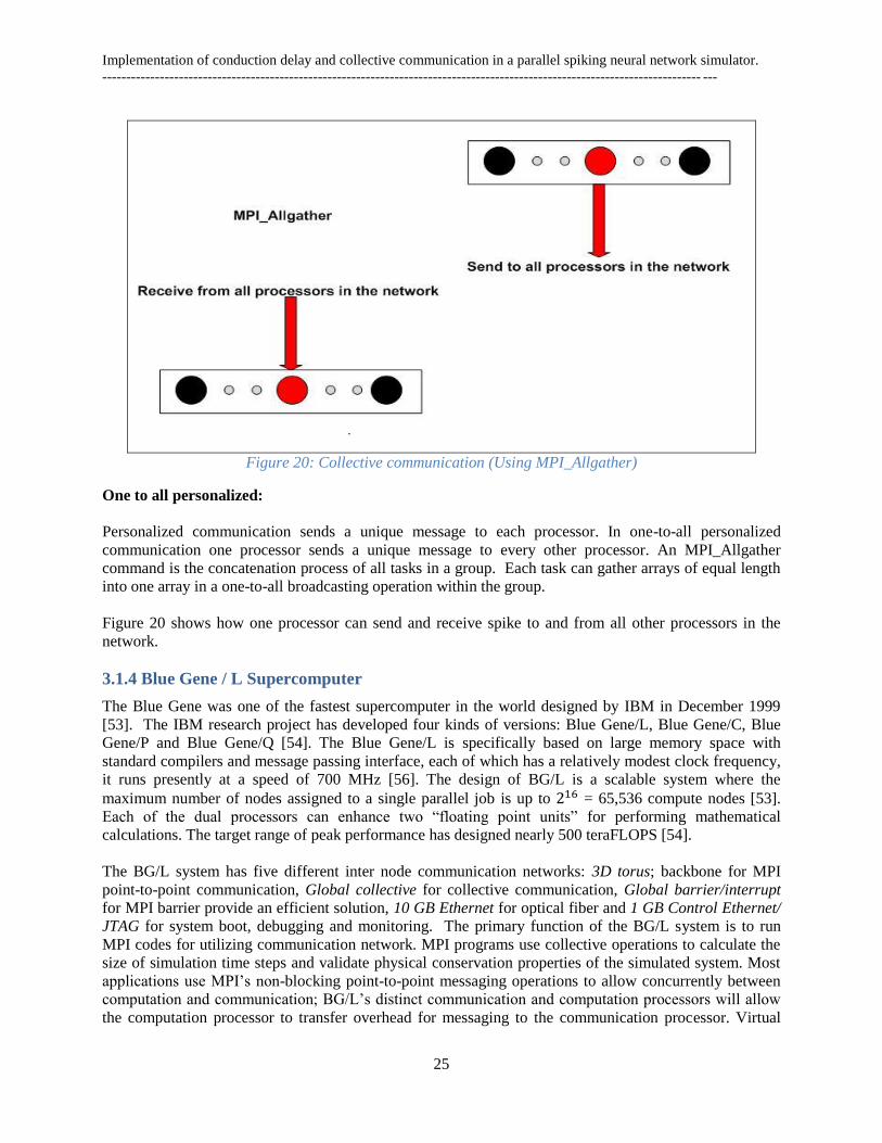
Figure 20: Collective communication (Using MPI_Allgather)
One to all personalized:
Personalized communication sends a unique message to each processor. In one-to-all personalized
communication one processor sends a unique message to every other processor. An MPI_Allgather
command is the concatenation process of all tasks in a group. Each task can gather arrays of equal length
into one array in a one-to-all broadcasting operation within the group.
Figure 20 shows how one processor can send and receive spike to and from all other processors in the
network.
3.1.4 Blue Gene / L Supercomputer
The Blue Gene was one of the fastest supercomputer in the world designed by IBM in December 1999
[53]. The IBM research project has developed four kinds of versions: Blue Gene/L, Blue Gene/C, Blue
Gene/P and Blue Gene/Q [54]. The Blue Gene/L is specifically based on large memory space with
standard compilers and message passing interface, each of which has a relatively modest clock frequency,
it runs presently at a speed of 700 MHz [56]. The design of BG/L is a scalable system where the
maximum number of nodes assigned to a single parallel job is up to = 65,536 compute nodes [53].
Each of the dual processors can enhance two “floating point units” for performing mathematical
calculations. The target range of peak performance has designed nearly 500 teraFLOPS [54].
The BG/L system has five different inter node communication networks: 3D torus; backbone for MPI
point-to-point communication, Global collective for collective communication, Global barrier/interrupt
for MPI barrier provide an efficient solution, 10 GB Ethernet for optical fiber and 1 GB Control Ethernet/
JTAG for system boot, debugging and monitoring. The primary function of the BG/L system is to run
MPI codes for utilizing communication network. MPI programs use collective operations to calculate the
size of simulation time steps and validate physical conservation properties of the simulated system. Most
applications use MPI‟s non-blocking point-to-point messaging operations to allow concurrently between
computation and communication; BG/L‟s distinct communication and computation processors will allow
the computation processor to transfer overhead for messaging to the communication processor. Virtual
Implementation of conduction delay and collective communication in a parallel spiking neural network simulator.
----------------------------------------------------------------------------------------------------------------------------- ---
26
mode and Co-processor mode is configured to run the BG/L system with two processors on a node run
simultaneously by allocating half of the memory space.
In my thesis, I am particularly familiar with Blue Gene/L machine which is provided by PDC, KTH. This
BG/L system has 1024 nodes and 2048 processors with 1 TB of memory [55]. The maximum simulations
designed in this thesis were executed on one BG/L machine comprising 2048 nodes.
3.1.5 JUGENE Supercomputer
Today‟s JUGENE is the fastest supercomputer in Europe introduced by Jülich, Germany. It is an IBM
supercomputer and offering the calculate power up to 1 PetaFLOPS [57]. This supercomputer
performance is capable of a massive one trillion computing operations per second and it is equipped with
294,912 processor cores [57]. About 72,000 nodes are housed in 72 water cooled racks [57].
3.2 Implementation of BCPNN
Here, we present the parallel implementation of the theoretical cortical model based on the BCPNN
learning rule. The BCPNN network is implemented as sparsely and randomly connection strength that is
based on the probabilities of the spiking activity. The network can be used in one of the two following
modes: learning and retrieval. In the learning stage, the network of all input pattern are connected and new
patterns are stored on top of the older ones as in palimpsest memory [58] so that weights are updated.
During retrieval stage, the network interprets the input pattern, using its internal representation or
knowledge.
The simplified learning rule of BCPNN has been implemented in our simulation. The computational
requirement of cortical model is largely dependent on total number of connections. The code is written in
C++ programming language with MPI communication routines, MPI_Allgather () and MPI_Isend () /
MPI_Irecv ().
3.2.1 The Hypercolumn Module
In our simulation, the number of units and connections in each hypercolumn is constant (100). The
performance of BCPNN network is depending on the hypercolumns and the number of hypercolumns was
fixed accordingly to 128, 256, 512, 1024 and 2048. The iteration times are also constant (0.0005s). The
iteration of the time step is done locally in each processing unit. Furthermore, the activity in each
hypercolumn in our model always sum to one. This means that our cortical model has a sparse activity
constant at 1% and achieved the perfect weak scaling.
Implementation of conduction delay and collective communication in a parallel spiking neural network simulator.
----------------------------------------------------------------------------------------------------------------------------- ---
27
Chapter 4: Results In this chapter, results are arranged in two sections. The first section contains the comparison between
point to point communications and collective communications. The second section contains only point to
point communications with delay and without delay.
In the result section, my aim is to show two different experiments and analyze their behavior by increasing
the hypercolumns such as 128, 256, 512, 1024 and 2048.
4.1 Communications Comparison
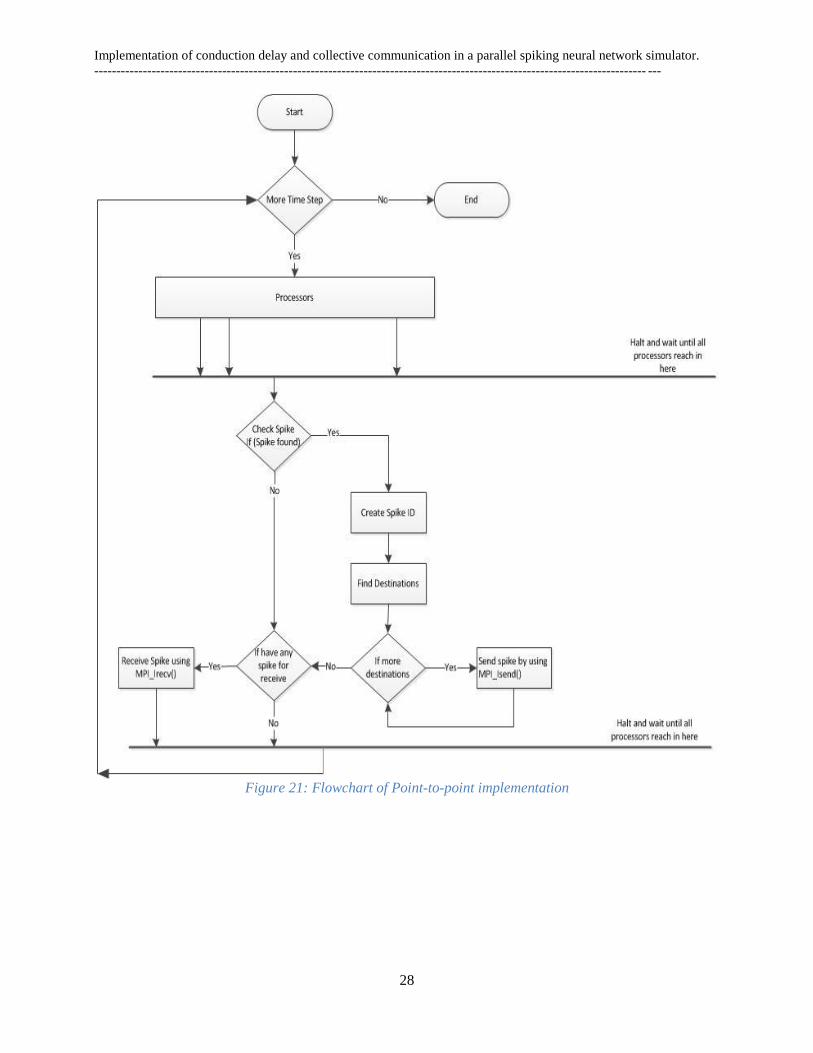
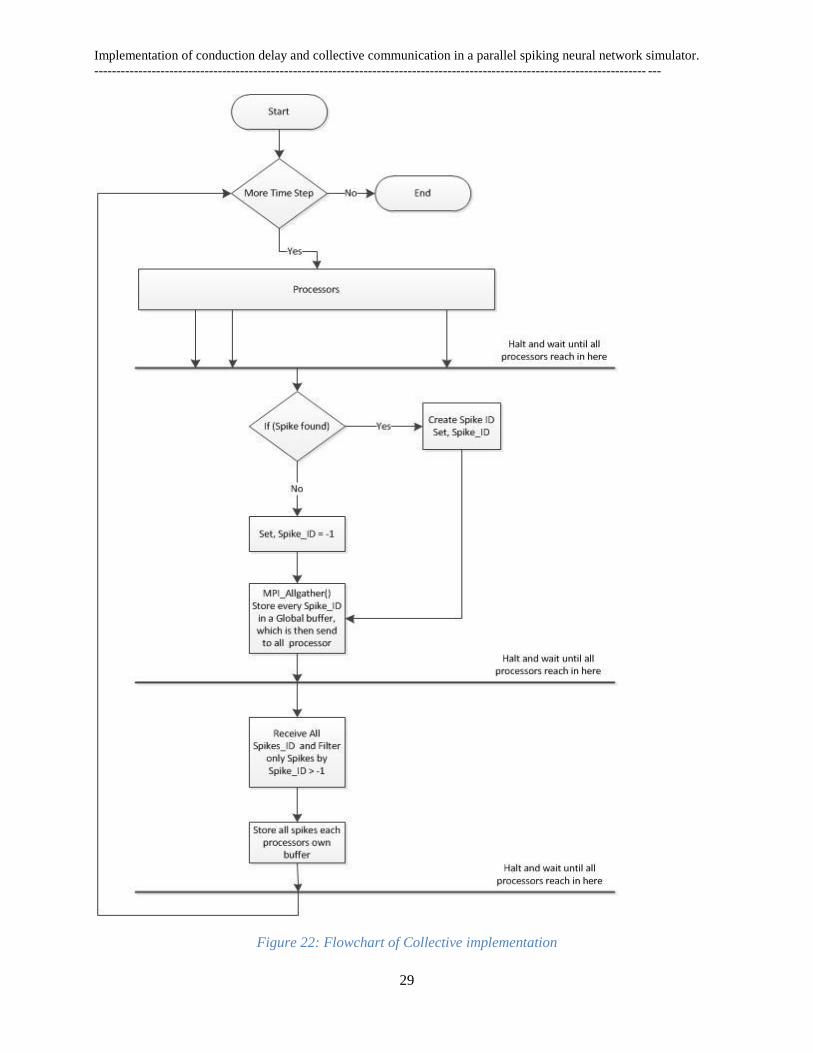
In this section, we present the comparison of results between point to point communications and collective
communications. But before that I would like to explain how communications have been implemented.
The flow chart of point-to-point and collective communications are shown below.
Implementation of conduction delay and collective communication in a parallel spiking neural network simulator.
----------------------------------------------------------------------------------------------------------------------------- ---
28
Figure 21: Flowchart of Point-to-point implementation
Implementation of conduction delay and collective communication in a parallel spiking neural network simulator.
----------------------------------------------------------------------------------------------------------------------------- ---
29
Figure 22: Flowchart of Collective implementation
Implementation of conduction delay and collective communication in a parallel spiking neural network simulator.
----------------------------------------------------------------------------------------------------------------------------- ---
30
The comparisons have been done through following five investigations.
4.1.1 Elapsed Time
The experiment was intended to compare the scaling capabilities and performance of MPI library with
communication functionality programmed in C++. The result will be presented in the following order.
First the elapsed times of overall network are presented and then the elapsed times for each loop are
shown.
Loop time = Elapsed time / Number of loops.
In our simulation, 100 patterns were trained and recalled.
Elapsed time of overall network
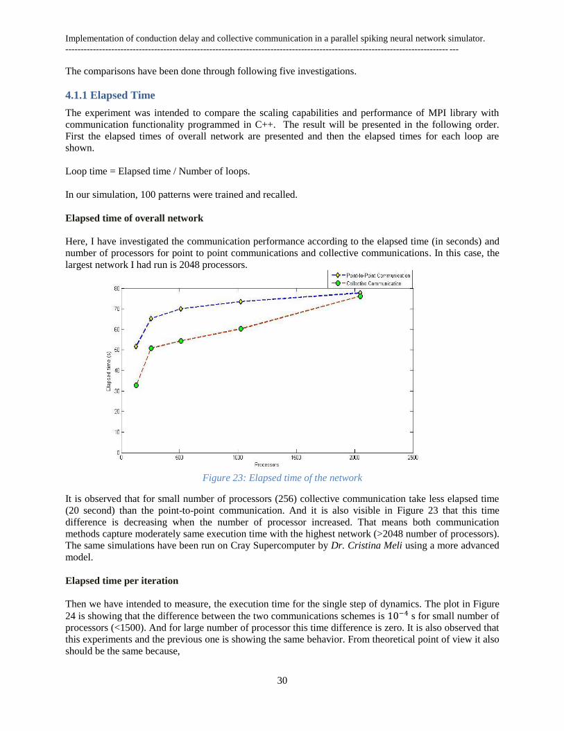
Here, I have investigated the communication performance according to the elapsed time (in seconds) and
number of processors for point to point communications and collective communications. In this case, the
largest network I had run is 2048 processors.
Figure 23: Elapsed time of the network
It is observed that for small number of processors (256) collective communication take less elapsed time
(20 second) than the point-to-point communication. And it is also visible in Figure 23 that this time
difference is decreasing when the number of processor increased. That means both communication
methods capture moderately same execution time with the highest network (>2048 number of processors).
The same simulations have been run on Cray Supercomputer by Dr. Cristina Meli using a more advanced
model.
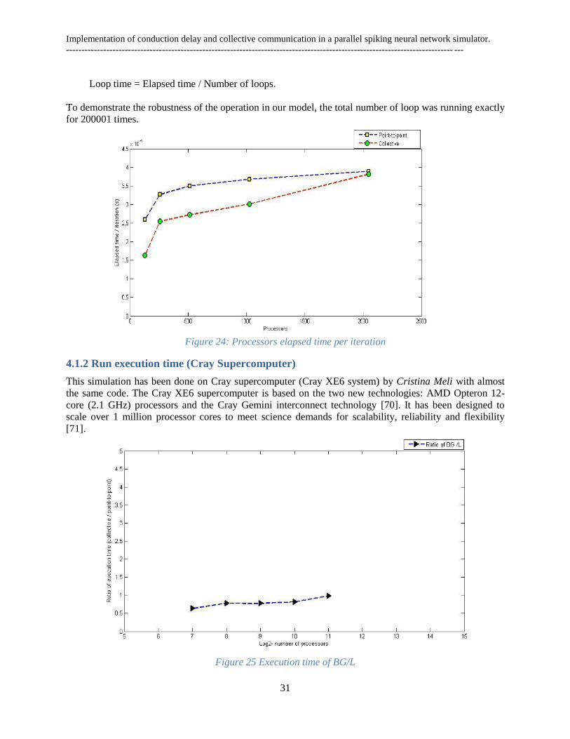
Elapsed time per iteration
Then we have intended to measure, the execution time for the single step of dynamics. The plot in Figure
24 is showing that the difference between the two communications schemes is s for small number of
processors (<1500). And for large number of processor this time difference is zero. It is also observed that
this experiments and the previous one is showing the same behavior. From theoretical point of view it also
should be the same because,
Implementation of conduction delay and collective communication in a parallel spiking neural network simulator.
----------------------------------------------------------------------------------------------------------------------------- ---
31
Loop time = Elapsed time / Number of loops.
To demonstrate the robustness of the operation in our model, the total number of loop was running exactly
for 200001 times.
Figure 24: Processors elapsed time per iteration
4.1.2 Run execution time (Cray Supercomputer)
This simulation has been done on Cray supercomputer (Cray XE6 system) by Cristina Meli with almost
the same code. The Cray XE6 supercomputer is based on the two new technologies: AMD Opteron 12-
core (2.1 GHz) processors and the Cray Gemini interconnect technology [70]. It has been designed to
scale over 1 million processor cores to meet science demands for scalability, reliability and flexibility
[71].
Figure 25 Execution time of BG/L
Implementation of conduction delay and collective communication in a parallel spiking neural network simulator.
----------------------------------------------------------------------------------------------------------------------------- ---
32
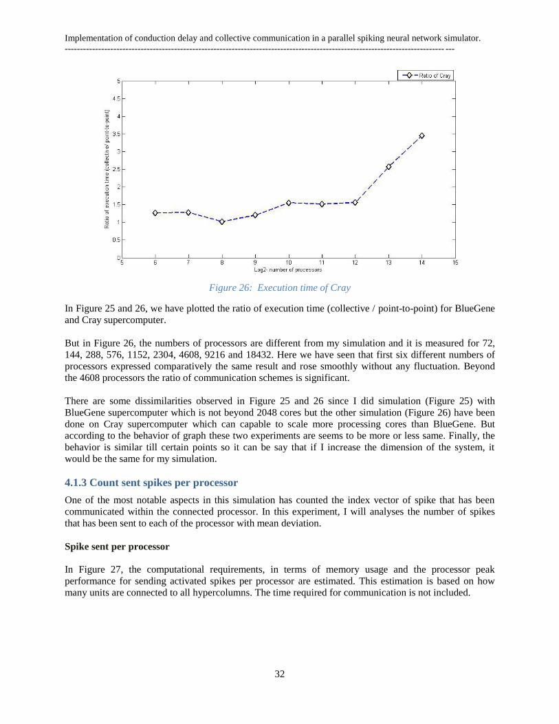
Figure 26: Execution time of Cray
In Figure 25 and 26, we have plotted the ratio of execution time (collective / point-to-point) for BlueGene
and Cray supercomputer.
But in Figure 26, the numbers of processors are different from my simulation and it is measured for 72,
144, 288, 576, 1152, 2304, 4608, 9216 and 18432. Here we have seen that first six different numbers of
processors expressed comparatively the same result and rose smoothly without any fluctuation. Beyond
the 4608 processors the ratio of communication schemes is significant.
There are some dissimilarities observed in Figure 25 and 26 since I did simulation (Figure 25) with
BlueGene supercomputer which is not beyond 2048 cores but the other simulation (Figure 26) have been
done on Cray supercomputer which can capable to scale more processing cores than BlueGene. But
according to the behavior of graph these two experiments are seems to be more or less same. Finally, the
behavior is similar till certain points so it can be say that if I increase the dimension of the system, it
would be the same for my simulation.
4.1.3 Count sent spikes per processor
One of the most notable aspects in this simulation has counted the index vector of spike that has been
communicated within the connected processor. In this experiment, I will analyses the number of spikes
that has been sent to each of the processor with mean deviation.
Spike sent per processor
In Figure 27, the computational requirements, in terms of memory usage and the processor peak
performance for sending activated spikes per processor are estimated. This estimation is based on how
many units are connected to all hypercolumns. The time required for communication is not included.
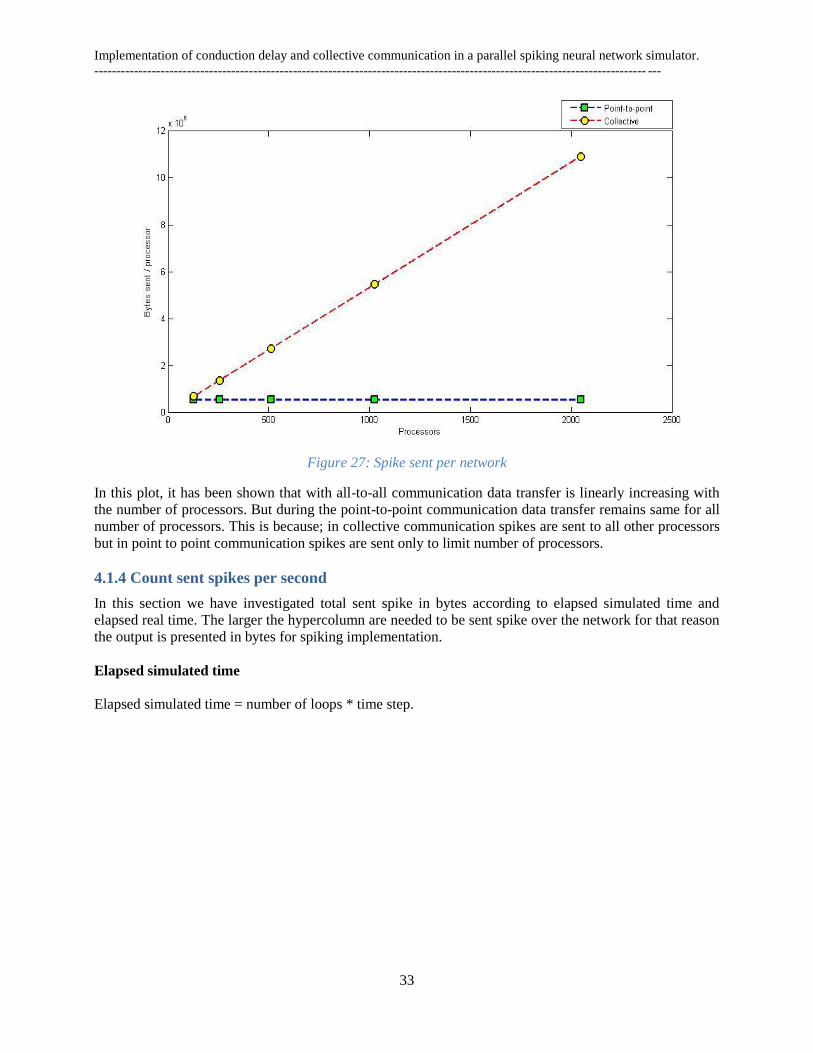
Implementation of conduction delay and collective communication in a parallel spiking neural network simulator.
----------------------------------------------------------------------------------------------------------------------------- ---
33
Figure 27: Spike sent per network
In this plot, it has been shown that with all-to-all communication data transfer is linearly increasing with
the number of processors. But during the point-to-point communication data transfer remains same for all
number of processors. This is because; in collective communication spikes are sent to all other processors
but in point to point communication spikes are sent only to limit number of processors.
4.1.4 Count sent spikes per second
In this section we have investigated total sent spike in bytes according to elapsed simulated time and
elapsed real time. The larger the hypercolumn are needed to be sent spike over the network for that reason
the output is presented in bytes for spiking implementation.
Elapsed simulated time
Elapsed simulated time = number of loops * time step.
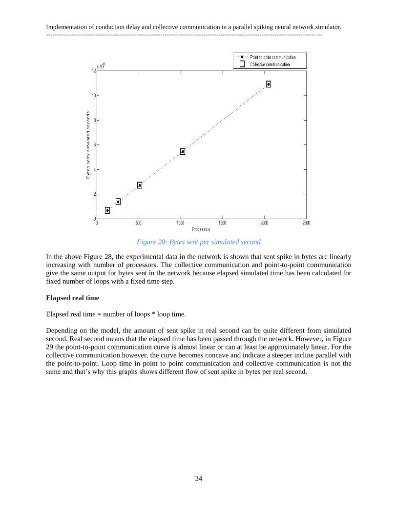
Implementation of conduction delay and collective communication in a parallel spiking neural network simulator.
----------------------------------------------------------------------------------------------------------------------------- ---
34
Figure 28: Bytes sent per simulated second
In the above Figure 28, the experimental data in the network is shown that sent spike in bytes are linearly
increasing with number of processors. The collective communication and point-to-point communication
give the same output for bytes sent in the network because elapsed simulated time has been calculated for
fixed number of loops with a fixed time step.
Elapsed real time
Elapsed real time = number of loops * loop time.
Depending on the model, the amount of sent spike in real second can be quite different from simulated
second. Real second means that the elapsed time has been passed through the network. However, in Figure
29 the point-to-point communication curve is almost linear or can at least be approximately linear. For the
collective communication however, the curve becomes concave and indicate a steeper incline parallel with
the point-to-point. Loop time in point to point communication and collective communication is not the
same and that‟s why this graphs shows different flow of sent spike in bytes per real second.
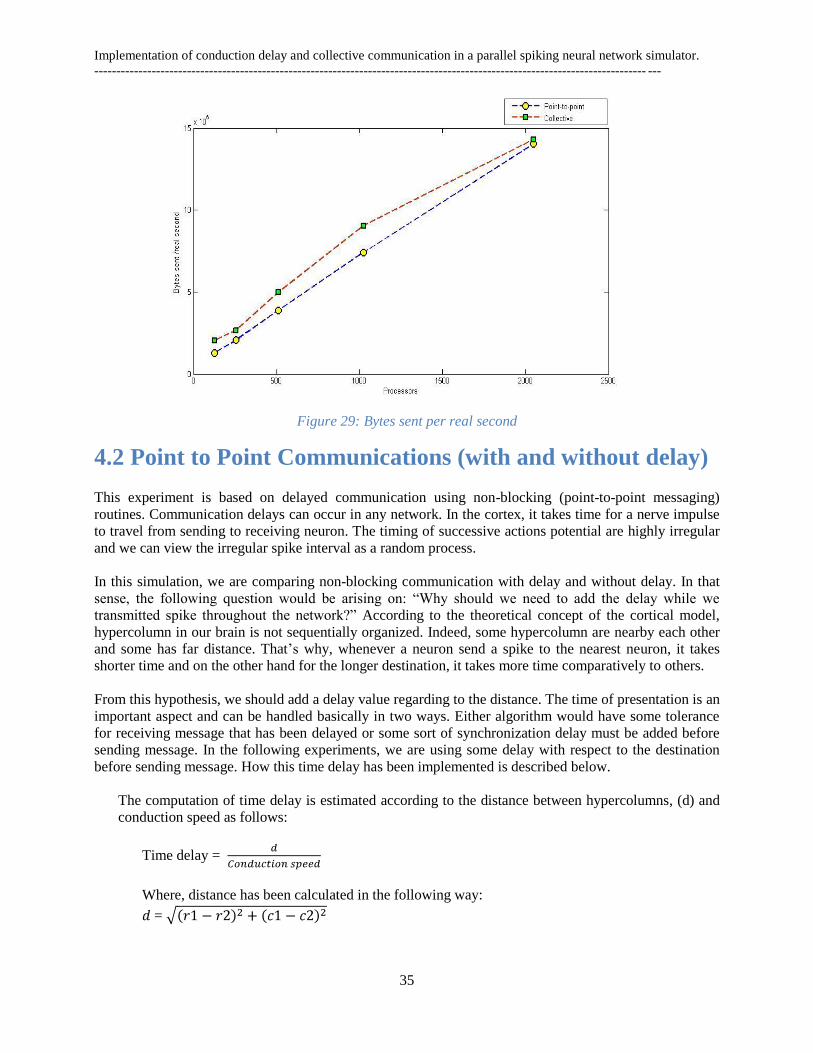
Implementation of conduction delay and collective communication in a parallel spiking neural network simulator.
----------------------------------------------------------------------------------------------------------------------------- ---
35
Figure 29: Bytes sent per real second
4.2 Point to Point Communications (with and without delay)
This experiment is based on delayed communication using non-blocking (point-to-point messaging)
routines. Communication delays can occur in any network. In the cortex, it takes time for a nerve impulse
to travel from sending to receiving neuron. The timing of successive actions potential are highly irregular
and we can view the irregular spike interval as a random process.
In this simulation, we are comparing non-blocking communication with delay and without delay. In that
sense, the following question would be arising on: “Why should we need to add the delay while we
transmitted spike throughout the network?” According to the theoretical concept of the cortical model,
hypercolumn in our brain is not sequentially organized. Indeed, some hypercolumn are nearby each other
and some has far distance. That‟s why, whenever a neuron send a spike to the nearest neuron, it takes
shorter time and on the other hand for the longer destination, it takes more time comparatively to others.
From this hypothesis, we should add a delay value regarding to the distance. The time of presentation is an
important aspect and can be handled basically in two ways. Either algorithm would have some tolerance
for receiving message that has been delayed or some sort of synchronization delay must be added before
sending message. In the following experiments, we are using some delay with respect to the destination
before sending message. How this time delay has been implemented is described below.
The computation of time delay is estimated according to the distance between hypercolumns, (d) and
conduction speed as follows:
Time delay =
Where, distance has been calculated in the following way:
=

Implementation of conduction delay and collective communication in a parallel spiking neural network simulator.
----------------------------------------------------------------------------------------------------------------------------- ---
36
And * diameter
of a hypercolumn
Here „ ‟ stands for distance, „r’ and „c’ is the co-ordinate of a hypercolumn.
Conduction speed is used in our simulation. Biologically, conduction speed means the speed of
electrical signal through a nerve.
As in this model, we have performed all necessary computation in training and retrieval phases in each
time step and the remaining communication is postponed at synchronization point. Although the range of
the distance in each hypercolumn is very small but in a large neural network the delay value gives some
slow response. Also it is essential to keep some physical velocity with the hypercolumn because it
accounts for irregular gap observed in real neurons.
As explained above, we can note two things. At first, I will Figure out the elapsed time is required both for
the network and for each processor even if some numerical value would be added. I will later compare the
experimental data of the sent spike as I did it before.
Again, before going to result analysis the implementation of time delay is shown below.
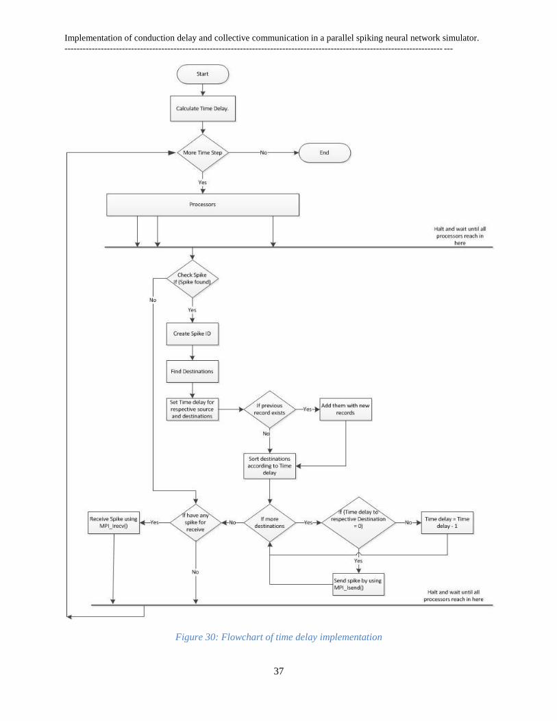
Implementation of conduction delay and collective communication in a parallel spiking neural network simulator.
----------------------------------------------------------------------------------------------------------------------------- ---
37
Figure 30: Flowchart of time delay implementation
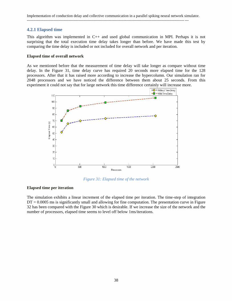
Implementation of conduction delay and collective communication in a parallel spiking neural network simulator.
----------------------------------------------------------------------------------------------------------------------------- ---
38
4.2.1 Elapsed time
This algorithm was implemented in C++ and used global communication in MPI. Perhaps it is not
surprising that the total execution time delay takes longer than before. We have made this test by
comparing the time delay is included or not included for overall network and per iteration.
Elapsed time of overall network
As we mentioned before that the measurement of time delay will take longer as compare without time
delay. In the Figure 31, time delay curve has required 20 seconds more elapsed time for the 128
processors. After that it has raised more according to increase the hypercolumn. Our simulation ran for
2048 processors and we have noticed the difference between them about 25 seconds. From this
experiment it could not say that for large network this time difference certainly will increase more.
Figure 31: Elapsed time of the network
Elapsed time per iteration
The simulation exhibits a linear increment of the elapsed time per iteration. The time-step of integration
DT = 0.0005 ms is significantly small and allowing for fine computation. The presentation curve in Figure
32 has been compared with the Figure 30 which is desirable. If we increase the size of the network and the
number of processors, elapsed time seems to level off below 1ms/iterations.
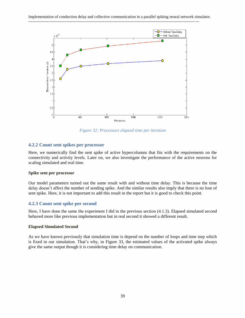
Implementation of conduction delay and collective communication in a parallel spiking neural network simulator.
----------------------------------------------------------------------------------------------------------------------------- ---
39
Figure 32: Processors elapsed time per iteration
4.2.2 Count sent spikes per processor
Here, we numerically find the sent spike of active hypercolumns that fits with the requirements on the
connectivity and activity levels. Later on, we also investigate the performance of the active neurons for
scaling simulated and real time.
Spike sent per processor
Our model parameters turned out the same result with and without time delay. This is because the time
delay doesn‟t affect the number of sending spike. And the similar results also imply that there is no lose of
sent spike. Here, it is not important to add this result in the report but it is good to check this point.
4.2.3 Count sent spike per second
Here, I have done the same the experiment I did in the previous section (4.1.3). Elapsed simulated second
behaved more like previous implementation but in real second it showed a different result.
Elapsed Simulated Second
As we have known previously that simulation time is depend on the number of loops and time step which
is fixed in our simulation. That‟s why, in Figure 33, the estimated values of the activated spike always
give the same output though it is considering time delay on communication.
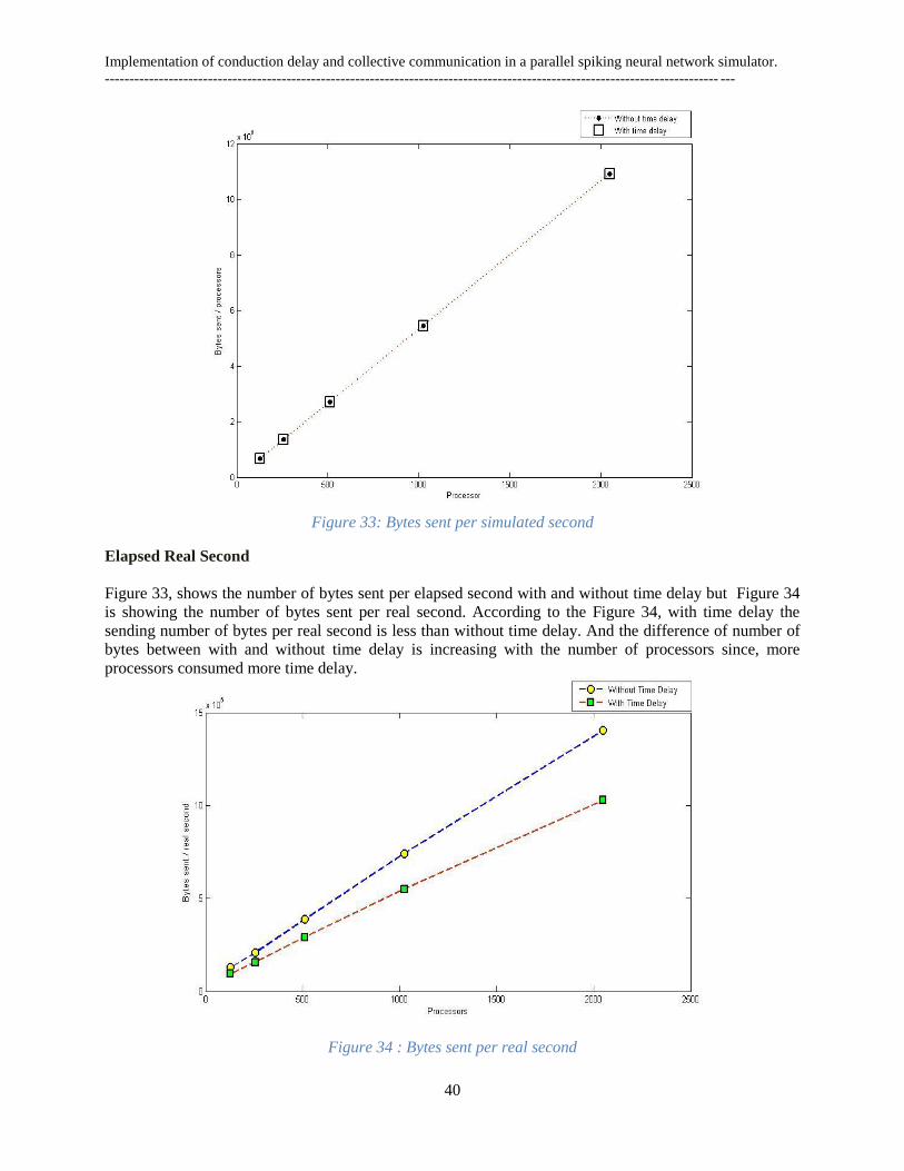
Implementation of conduction delay and collective communication in a parallel spiking neural network simulator.
----------------------------------------------------------------------------------------------------------------------------- ---
40
Figure 33: Bytes sent per simulated second
Elapsed Real Second
Figure 33, shows the number of bytes sent per elapsed second with and without time delay but Figure 34
is showing the number of bytes sent per real second. According to the Figure 34, with time delay the
sending number of bytes per real second is less than without time delay. And the difference of number of
bytes between with and without time delay is increasing with the number of processors since, more
processors consumed more time delay.
Figure 34 : Bytes sent per real second
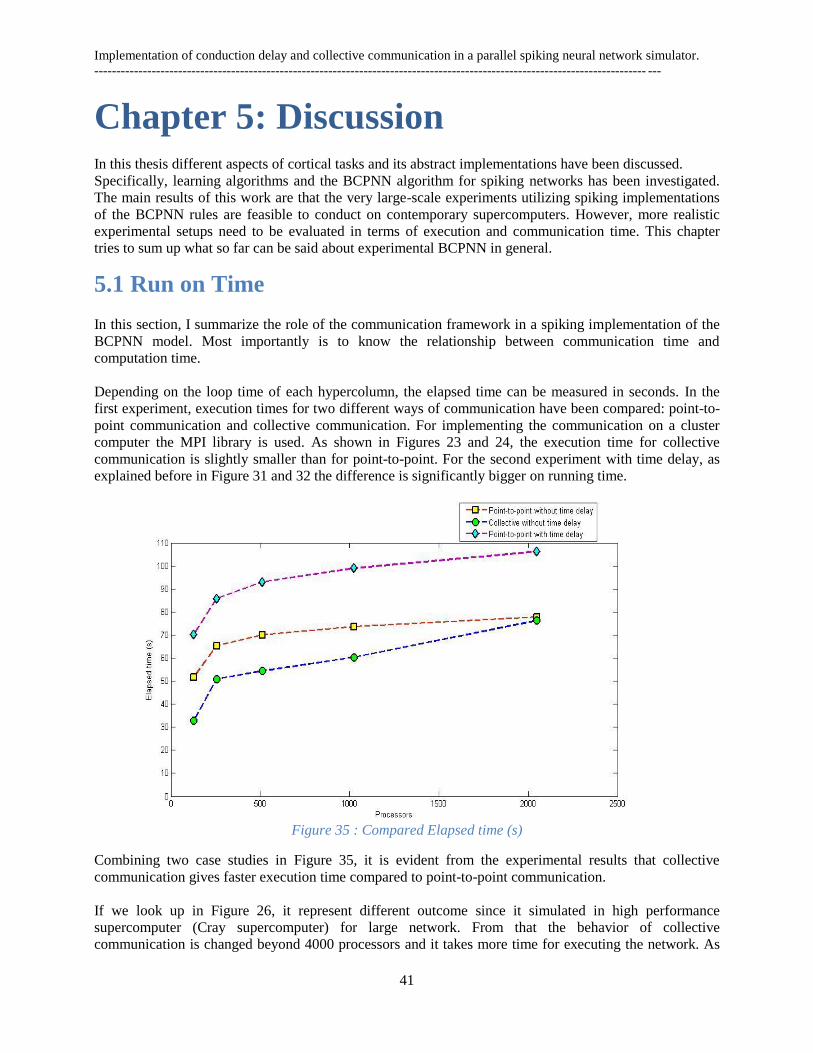
Implementation of conduction delay and collective communication in a parallel spiking neural network simulator.
----------------------------------------------------------------------------------------------------------------------------- ---
41
Chapter 5: Discussion In this thesis different aspects of cortical tasks and its abstract implementations have been discussed.
Specifically, learning algorithms and the BCPNN algorithm for spiking networks has been investigated.
The main results of this work are that the very large-scale experiments utilizing spiking implementations
of the BCPNN rules are feasible to conduct on contemporary supercomputers. However, more realistic
experimental setups need to be evaluated in terms of execution and communication time. This chapter
tries to sum up what so far can be said about experimental BCPNN in general.
5.1 Run on Time
In this section, I summarize the role of the communication framework in a spiking implementation of the
BCPNN model. Most importantly is to know the relationship between communication time and
computation time.
Depending on the loop time of each hypercolumn, the elapsed time can be measured in seconds. In the
first experiment, execution times for two different ways of communication have been compared: point-to-
point communication and collective communication. For implementing the communication on a cluster
computer the MPI library is used. As shown in Figures 23 and 24, the execution time for collective
communication is slightly smaller than for point-to-point. For the second experiment with time delay, as
explained before in Figure 31 and 32 the difference is significantly bigger on running time.
Figure 35 : Compared Elapsed time (s)
Combining two case studies in Figure 35, it is evident from the experimental results that collective
communication gives faster execution time compared to point-to-point communication.
If we look up in Figure 26, it represent different outcome since it simulated in high performance
supercomputer (Cray supercomputer) for large network. From that the behavior of collective
communication is changed beyond 4000 processors and it takes more time for executing the network. As
Implementation of conduction delay and collective communication in a parallel spiking neural network simulator.
----------------------------------------------------------------------------------------------------------------------------- ---
42
we know previously (chapter 3) collective communication is responsible to send all messages to the whole
network. So it can be say that it is obvious to take more time for large network in collective
communication.
At a first glance, the point-to-point communication with time delay require more time while running the
network. The question whether it is feasible to simulate networks making use of artificial time delay is
important, because in real neural networks communication delays depend on the distance of two
connected neurons among other things. It can be concluded here, that it is feasible to use artificial
communication delay in the networks that have been studied. So communication with time delay is
completely feasible.
The estimate on running times to the network is concluded that the communications protocol should
become the bottleneck in a large scale simulation using collective communication.
5.2 Activity of sent spike
The BCPNN algorithm is compared to other algorithms computationally expensive (see Chapter 2). Due
to the large computational requirements the memory usage also is high, computational times are mostly
depend on the speed and number of processors used.
The architecture of the network is also a matter of concern. In Figure 27, point-to-point communication
has to be taken a fairly straight result. But we have seen a dramatically increase in collective
communication. It is proved from the experimental result that the amount of information broadcasted is
huge and apparently most of it is not necessary.
It would be valuable to exhibit the active spike data over simulated and real time (see Chapter 4). During
simulated time both experiments show the same result. It gives a very good quantitative fit to the data
meaning that out spiking connectivity rule is robust. But when we calculate the amount of sent spike on
real time then collective communication takes more spikes compare to point to point communication.
Implementation of conduction delay and collective communication in a parallel spiking neural network simulator.
----------------------------------------------------------------------------------------------------------------------------- ---
43
Chapter 6: Conclusion In this master thesis project, we have learned an adaptation of the mammalian cortex to come up with an
abstract BCPNN model for spiking units. There has been a strong motivation to have increased its
computational capabilities. We expect further developments of this model and also will make a thorough
analysis of the implications and requirements on the communications.
Our work present results in brain-inspired algorithm and gives a computational account for neural
communication. Instead of testing synaptic connection and learning rule in a network context, we have
focused on large-scale network in parallel environment in order to make a strong contribution in modular
structure of neocortex.
The BCPNN model has been developed for many years and the work in this thesis followed up on the
directions proposed in the doctoral thesis by Christopher Johansson (2006) to implement a BCPNN of P-
type. My co-supervisor Cristina Meli expects the further development of a Z-type BCPNN with an
intermediate level of complexity.
Everyday a new and higher performing supercomputer sets its foot on the market and provides more
computing power and more memory. For the purpose of simulating a cortical sized BCPNN in real time
on a cluster with thousands of nodes, faster communications are needed and less execution time required. I
am positive that continued this work will be a source of reward for the next years to come.
Implementation of conduction delay and collective communication in a parallel spiking neural network simulator.
----------------------------------------------------------------------------------------------------------------------------- ---
44
References 1. Dale Purves, George J. Augustine, David Fitzpatrick, William C. Hall, Anthony-Samuel LaMantia,
James O. McNamara, S. Mark Williams (2004): Neuroscience (3rd
Edition), Publisher: Sinauer
Associates, Inc, Sunderland, Massachusetts, USA. ISBN 0-87893-725-0
2. Patric Hagmann, Lelia Cammoun, Xavier Gigandet , Reto Meuli, Christopher J. Honey, Van J.
Wedeen and Olaf Sporns (2008)-Mapping the structural core of human cerebral cortex. PLoS Biol
6(7): e159. doi:10.1371/journal.pbio.0060159
3. Eric R. Kandel, James H. Schwartz, Thomas M. Jessell (1995): Essential of Neuroscience and
Behavior ,Publisher: Appleton & Lange, ISBN 0-8385-2245-9 (p-184,187)
4. Joanna Gilbert, “Biology Mad”, the Human Nervous System. Bibliographies and Web Indexes, K-12
Curriculum and Lesson Plans, Presentations, NBII.
5. Rawland Hall, “AP Psychology“, Handouts, Unit 5: Neuroscience
(http://www.rhsmpsychology.com/Handouts/Neuroscience_handouts.htm).
6. Maria Victoria,(2001)”Biology Online” Tutorial: Human Neurology; (http://www.biology-
online.org/8/1_nervous_system.htm)
7. Auke Jan Ijspeert, Toshimitsu Masuzawa and Shinji Kusumoto (2006),” Biologically inspired
approaches to advanced information technology” Publisher: SpringerLink , ISBN: 3540312536
8. Jarvis ED, Gunturkun O, Bruce L, Csillag A, Karten H, Kuenzel W, Medina L, Paxinos G, Perkel DJ,
Shimizu T, Striedter G, Wild JM, Ball GF, Dugas-Ford J, Durand SE, Hough GE, Husband S,
Kubikova L, Lee DW, Mello CV, Powers A, Siang C, Smulders TV, Wada K, White SA, Yamamoto
K, Yu J, Reiner A, Butler AB (2005): Avian brains and a new understanding of vertebrate brain
evolution. Nature Reviews Neuroscience 6, (151-159 ) doi:10.1038/nrn1606
9. Christopher Johansson and Anders Lansner (2004): “Towards Cortex Sited Attractor ANN”.
Knowledge-Based International and Engineering System- KES‟04, Willington, New Zealand, LNAI
3213. Publisher: Elsevier Ltd, doi:10.1016/j.neunet.2006.05.029
10. Rockel AJ, Hiorns RW, Powell TP (2004): “The basic uniformity in structure of the neocortex”. Brain
(1980) 103 (2): 221-244. doi: 10.1093/brain/103.2.221
11. Christopher Johansson, October 2006- “An attractor memory model of neocortex “(Doctoral thesis),
p.42. 49. 51,ISBN: 91-7178-461-6,TRITA-CSC-A-2006.14,ISSN-1653-5723,ISRN-KTH/SCS/A-
06/14.SE
12. Christopher Johansson and Anders Lansner (2006). “A Hierarchical Brain Inspired Computing
Systems”. In Proc. International Symposium on Nonlinear Theory and its Application- NOLTA‟06.
13. Christopher Johansson and Anders Lansner (2001)"A Parallel Implementation of a Bayesian Neural
Network with Hypercolumns", TRITA-NA-P0121, ISSN 1101-2250 ,ISRN KTH/NA/P-01/21S
14. Kendra Cherry, (2005),”What is a neuron?” About.com, A part of The New York Times Company

Implementation of conduction delay and collective communication in a parallel spiking neural network simulator.
----------------------------------------------------------------------------------------------------------------------------- ---
45
15. Neural Networks (Middle school level, The American physiological society) Developed by the
Columbus, OH local outreach team
16. Daniel Rios, ”Neuro AI” (2007-2010),Artificial neural network- A neural network tutorial.
17. http://bio1152.nicerweb.com/Locked/media/ch48/cerebral.html
18. Jonathan C. Horton and Daniel L. Adams (April, 2005). “The cortical column: a structure without a
function”. Philos Trans R Soc Lond B Biol Sci; 360(1456): 837–862.
19. Daniel Y. Ts‟o, Mark Zarella and Guy Burkitt (2009). “Whither the hypercolumn?”
doi:10.1113/jphysiol.2009.171082 June 15,The Journal of Physiology, 587, 2791-2805
20. Daniel P. Buxhoeeveden and Manual F. Casanova (2002). “The minicolumn hypothesis in
neuroscience”. Brain, 125 (5): 935-951. doi: 10.1093/brain/awf110
21. Baran Çürüklü and Anders Lansner (2002). “An Abstract Model of a Cortical Hypercolumn”. In
proceedings of the 9th International Conference on Neural Information Processing (ICONIP), pp. 80–
85, Singapore, IEEE Press.
22. http://imueos.blogspot.com/2010/10/organization-of-cerebral-cortex.html
23. Hebb, D.O., 1949: “The Organization of Behavior”. New York: John Wiley Inc
24. Anders Lansner and Erik Fransén (1998) – “Attractor Network Models of Cortical Associative
Memory”. Biocomputing and emergent computation: Proceedings of BCEC97,World Scientific press
25. Christopher Johansson, Anders Lansner and Erik Fransén (2002): Cell Assembly Dynamics in
Detailed and Abstract Attractor Models of Cortical Associative Memory. (SANS) Volume 122, Issue
1, Pages 19-36, doi:10.1078/1431-7613-00072, Published by Elsevier GmbH.
26. Simon Haykin (1999): Neural Networks- A Comprehensive Foundation. (2nd
Edition) Prientice-Hall
Inc.
27. Schoenauer Marc, Equipe Evolution Artificielle et Apprentissage de l‟x, Université Paris Sud,
(September 2007),( http://www.lri.fr/~marc/EEAAX/Neurones/tutorial/aneuron/html/index.html)
28. Hopfield J.J., (April 1982): “Neural networks and physical systems with emergent collective
computational properties”, PNAS vol. 79, no.8, pp. 2554-2558.
29. S. Haykin. Neural Networks - A comprehensive foundation. Prentice Hall International, Inc,
2nd edition, 1999. ISBN 0 13 908385 5.
30. Willshaw, D. J., Buneman, O. P., & Longuet-Higgins, H. C. (1969). Non-holographic associative
memory. Nature, 222(5197), 960-962.
31. Palm, G. (1980). On associative memory. Biological Cybernetics, 36(1), p.19-31.
32. Farooq Azam, (May-2000) –“Biologically Inspired Modular Neural Networks” (Doctoral Thesis).
p.12-32. Publisher: Citeseer, Pages: 149
Implementation of conduction delay and collective communication in a parallel spiking neural network simulator.
----------------------------------------------------------------------------------------------------------------------------- ---
46
33. Christopher Johansson and Anders Lansner (2006) – “Mapping of the BCPNN onto Cluster
Computers”. ISSN 1101-2250. TRITA-NA-P0305. SANS.
34. Christopher Johansson and Anders Lansner (2006)- “Attractor Memory with Self-organizing Input”.
A.J. Ijspeert et al. (Eds.): BioADIT, LNCS 3853.p-265-280.
35. A. Sandberg, A. Lansner, K.M. Peterson, and O. Ekeberg. “A palimpsest memory based on an
incremental learning rule”. Neurocomputing, pages 997–994, 2000.
36. MPI: “A Messaging Passing Interface Standard”, 1995, University of Tennessee, Knoxville,
Tennessee.
37. http://blogs.ubc.ca/psyc207/2011/01/19/neurons-how-do-they-communicate/
38. http://bio1152.nicerweb.com/Locked/media/ch48/cerebral.html
39. http://andreeasanatomy.blogspot.com/2011/04/you-need-to-step-up-on-step-to-reach_23.html
40. IBM System Blue Gene Solution: Application Development- An IBM Redbooks publication
41. Paul Burton (February 2009);An introduction to MPI programming, Organizer: ECMWF
42. Blaise Barney;” Message Passing Interface (MPI)”, , Lawrence Livermore National Laboratory UCRL-MI-133316
43. PDC center for high performance computing- MPI
(http://www.pdc.kth.se/education/historical/previous-years-summer-
schools/2009/handouts/lect2.pdf/view)
44. William Gropp, Ewing Lusk, and Anthony Skjellum (1991); “Using MPI: Portable Parallel
Programming with the Message-Passing Interface”, Published: MIT Press, ISBN 0-262-57133-1
45. M Snir, SW Otto, S Huss-Lederman, DW Walker, J (1998) MPI—The Complete Reference: Volume 1,
The MPI Core. MIT Press, Cambridge, MA. ISBN 0-262-69215-5
46. Argo Beowulf Cluster: MPI Commands and Examples, Organizer: ACCC Systems Group.(modified
2010-1-28)
47. Overview of Intro to MPI class-Organizer: Dartmouth College( modified February 14, 2011)
48. William Gropp-Tutorial on MPI: The Message-Passing Interface; Mathematics and Computer
Science Division ,Argonne National Laboratory
49. Scientific Computation , General Online Tutorials- The Message Passing Interface (MPI) Workshop;
University of Minnesota, Supercomputing Institute
50. MPI ,C++ Examples (http://people.sc.fsu.edu/~jburkardt/cpp_src/mpi/mpi.html)
51. Cristopher Johansson, Orjan Ekeberg, Anders Lansner (2006)-“Clustering of stored memories in an
attractor network with local competition ” International Journal of Neural Systems, 16(6): 393-40.
52. C++ Language Tutorial
Implementation of conduction delay and collective communication in a parallel spiking neural network simulator.
----------------------------------------------------------------------------------------------------------------------------- ---
47
53. The Blue Gene/L Team and IBM and Lawrence Livermore National Laboratory (2002): “An
Overview of the Blue Gene/L supercomputer” 0-7695-1524-X/02 $17.00 (c) 2002 IEEE.
54. From Wikipedia, the free encyclopedia, Blue Gene.
55. http://www.pdc.kth.se/resources/computers/bluegene/hebb-description
56. Blaise Barney, Lawrence Livermore National Laboratory, tutorial , „Using the Dawn BG/P System’,
LLNL-WEB-412512
57. From Wikipedia, the free encyclopedia, JUGENE.
58. J .P. Nadal, G. Toulou, et al. (1986): “Networks of Formal Neurons and Memory Palimpsests”.
Europhysics Letters ,1(10): 535-542
59. Christopher Johansson, Martin Rehn and Anders Lansner (2005 Elsevier); “Attractor Neural Networks
with Patchy Connectivity”. Neurocomputing 69 (2006) 627-633. ISBN: 0925-2312
60. Richard B. Well, April, 2005,” Cortical Neurons and Circuits: A Tutorial Introduction”. LCNTR
Tech Brief Moscow ID, the University of Idaho.
61. Richard H. Granger and Robert A. Hearn (2007), “Model of the thalamocortical System”
Scholarpedia, 2(11):1796.
62. http://www.dermaestetica.es/avanzes/blood.php?q=the-main-parts-of-the-brain&page=3
63. Hossein Bidgoli, 2010, “The Handbook of Technology Management”, Vol-3, Hoboken, N.J.: Wiley,
c2010.p-548.
64. Bechtel, W., & Abrahamsen, A. (2002).” Connectionism and the mind”. Second edition, Oxford, UK:
Blackwell.
65. H. Siegelman and S. Fishman. “Attractor systems and analog computation”. In Second Int. Conf. on
Knowledge-Based Intelligent Systems, pages 237–242, April 1998.
66. http://en.wikipedia.org/wiki/Neocortex
67. http://en.wikipedia.org/wiki/Cortical_column
68. Christopher Johansson and Anders Lansner (2005), "A Mean Field Approximation of
BCPNN",TRITA-NA-P0506, Department of Numerical Analysis and Computer Science, Royal
Institute of Technology
69. John A. Hertz, Anders S. Krogh and Richard G. Palmer (1991), “Introduction to the theory of neural
computation”, Addison-Wesely, Elsevier Science Publishers, ISBN 0-201-51560-1. (Library of
Congress: QA76.5.H475).
70. http://www.pdc.kth.se/resources/computers/lindgren
71. http://investors.cray.com/phoenix.zhtml?c=98390&p=irol-newsArticle&ID=1430648&highlight=
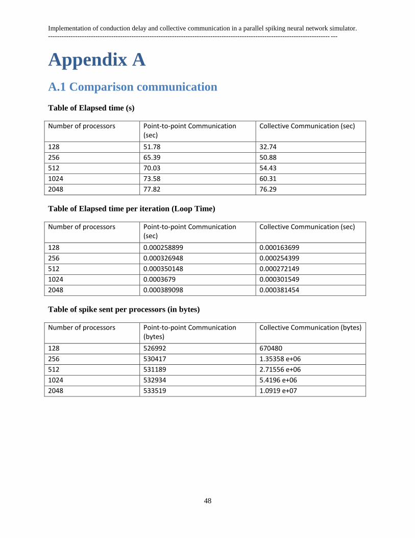
Implementation of conduction delay and collective communication in a parallel spiking neural network simulator.
----------------------------------------------------------------------------------------------------------------------------- ---
48
Appendix A
A.1 Comparison communication
Table of Elapsed time (s)
Number of processors Point-to-point Communication (sec)
Collective Communication (sec)
128 51.78 32.74
256 65.39 50.88
512 70.03 54.43
1024 73.58 60.31
2048 77.82 76.29
Table of Elapsed time per iteration (Loop Time)
Number of processors Point-to-point Communication (sec)
Collective Communication (sec)
128 0.000258899 0.000163699
256 0.000326948 0.000254399
512 0.000350148 0.000272149
1024 0.0003679 0.000301549
2048 0.000389098 0.000381454
Table of spike sent per processors (in bytes)
Number of processors Point-to-point Communication (bytes)
Collective Communication (bytes)
128 526992 670480
256 530417 1.35358 e+06
512 531189 2.71556 e+06
1024 532934 5.4196 e+06
2048 533519 1.0919 e+07
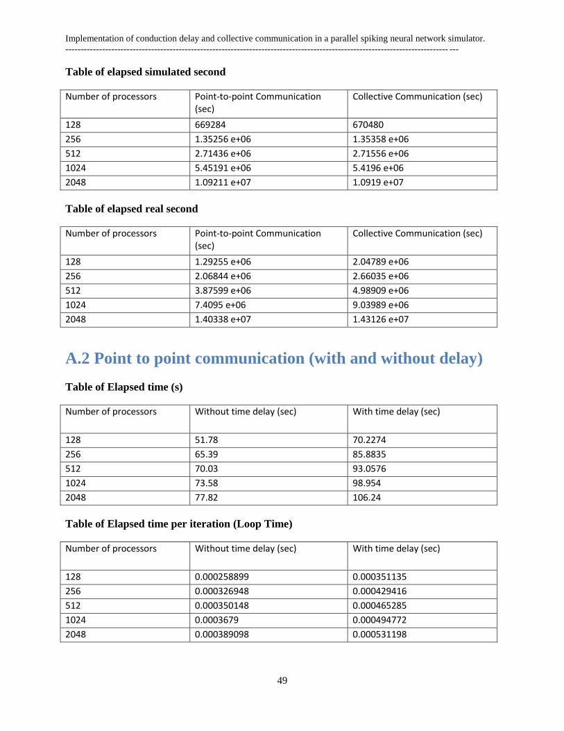
Implementation of conduction delay and collective communication in a parallel spiking neural network simulator.
----------------------------------------------------------------------------------------------------------------------------- ---
49
Table of elapsed simulated second
Number of processors Point-to-point Communication (sec)
Collective Communication (sec)
128 669284 670480
256 1.35256 e+06 1.35358 e+06
512 2.71436 e+06 2.71556 e+06
1024 5.45191 e+06 5.4196 e+06
2048 1.09211 e+07 1.0919 e+07
Table of elapsed real second
Number of processors Point-to-point Communication (sec)
Collective Communication (sec)
128 1.29255 e+06 2.04789 e+06
256 2.06844 e+06 2.66035 e+06
512 3.87599 e+06 4.98909 e+06
1024 7.4095 e+06 9.03989 e+06
2048 1.40338 e+07 1.43126 e+07
A.2 Point to point communication (with and without delay)
Table of Elapsed time (s)
Number of processors Without time delay (sec) With time delay (sec)
128 51.78 70.2274
256 65.39 85.8835
512 70.03 93.0576
1024 73.58 98.954
2048 77.82 106.24
Table of Elapsed time per iteration (Loop Time)
Number of processors Without time delay (sec) With time delay (sec)
128 0.000258899 0.000351135
256 0.000326948 0.000429416
512 0.000350148 0.000465285
1024 0.0003679 0.000494772
2048 0.000389098 0.000531198
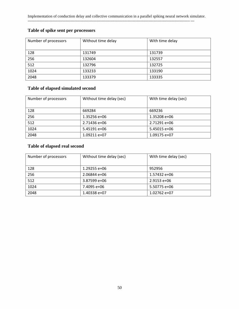
Implementation of conduction delay and collective communication in a parallel spiking neural network simulator.
----------------------------------------------------------------------------------------------------------------------------- ---
50
Table of spike sent per processors
Number of processors Without time delay With time delay
128 131749 131739
256 132604 132557
512 132796 132725
1024 133233 133190
2048 133379 133335
Table of elapsed simulated second
Number of processors Without time delay (sec) With time delay (sec)
128 669284 669236
256 1.35256 e+06 1.35208 e+06
512 2.71436 e+06 2.71291 e+06
1024 5.45191 e+06 5.45015 e+06
2048 1.09211 e+07 1.09175 e+07
Table of elapsed real second
Number of processors Without time delay (sec) With time delay (sec)
128 1.29255 e+06 952956
256 2.06844 e+06 1.57432 e+06
512 3.87599 e+06 2.9153 e+06
1024 7.4095 e+06 5.50775 e+06
2048 1.40338 e+07 1.02762 e+07

Implementation of conduction delay and collective communication in a parallel spiking neural network simulator.
----------------------------------------------------------------------------------------------------------------------------- ---
51
-END-

TRITA-CSC-E 2011:134 ISRN-KTH/CSC/E--11/134-SE
ISSN-1653-5715
www.kth.se