implementation of polar wrf for short range prediction of

Implementation of Polar WRF for short range predictionof weather over Maitri region in Antarctica

Anupam Kumar1,2, S K Roy Bhowmik

1,∗ and Ananda K Das1

1India Meteorological Department, New Delhi 110 003, India.2Present affiliation: Asia Risk Centre (an affiliate of RMS), Noida, U.P., India.∗Corresponding author. e-mail: [email protected] [email protected]

India Meteorological Department has implemented Polar WRF model for the Maitri (lat. 70◦45′S,long. 11◦44′E) region at the horizontal resolution of 15 km using initial and boundary conditions of theGlobal Forecast System (GFS T-382) operational at the India Meteorological Department (IMD). Mainobjective of this paper is to examine the performance skill of the model in the short-range time scaleover the Maitri region. An inter-comparison of the time series of daily mean sea level pressure and sur-face winds of Maitri for the 24 hours and 48 hours forecast against the corresponding observed fields hasbeen made using 90 days data for the period from 1 December 2010 to 28 February 2011. The resultreveals that the performance of the Polar WRF is reasonable, good and superior to that of IMD GFSforecasts. GFS shows an underestimation of mean sea level pressure of the order of 16–17 hPa with rootmean square errors (RMSE) of order 21 hPa, whereas Polar WRF shows an overestimation of the orderof 3–4 hPa with RMSE of 4 hPa. For the surface wind, GFS shows an overestimation of 1.9 knots at 24hours forecast and an underestimation of 3.7 knots at 48 hours forecast with RMSE ranging between 8and 11 knots. Whereas Polar WRF shows underestimation of 1.4 knots and 1.2 knots at 24 hours and 48hours forecast with RMSE of 5 knots. The results of a case study illustrated in this paper, reveal thatthe model is capable of capturing synoptic weather features of Antarctic region. The performance of themodel is found to be comparable with that of Antarctic Meso-scale Prediction System (AMPS) products.

1. Introduction

The Indian Antarctic program is a multi-disciplinary and multi-institutional program underthe control of the National Centre for Antarc-tic and Ocean Research. It was initiated in 1981with the first Indian expedition to Antarctica.Under the program (Pandey 2007), atmospheric,biological, earth, chemical and medical sciences arebeing studied by India. The first permanent set-tlement was built in 1983 at Dakshin Gangotri(lat. 70◦45′S, long. 12◦30′E). In 1989 it was aban-doned after it got buried in ice and Maitri base

(lat. 70◦45′S, long. 11◦44′E) was constructed in1990. Recently, India has constructed another newbase called ‘Lawrence Hills’, located at lat. 69◦24′S,long. 76◦11′E. The new base is now named as‘Bharati’.

Antarctica (Schwedtfeger 1984) is the coldest,windiest, highest, driest, and iciest continent onEarth. The general circulation pattern has thewinds moving coastward from the polar plateau,turning left under the effect of the Coriolis forceand merging with the coastal polar easterlies.Katabatic flow of Antarctica region is well knownfor producing extremely strong sustained winds.

Keywords. Numerical weather prediction; Polar WRF; polar meteorology.

J. Earth Syst. Sci. 121, No. 5, October 2012, pp. 1125–1143c© Indian Academy of Sciences 1125

1126 Anupam Kumar et al.

Blizzards are a typical Antarctic phenomenonoccurring when drift snow is picked up and blownalong the surface by the violent winds. A severeblizzard may last for a week at a time with windsblasting at over 100 miles/hour. One of the mostremarkable features of the sub–Antarctic latitudesis the high frequency of cyclonic storms, manyof which are intense. These systems have a largeimpact on weather in the region and particularlyat coastal locations, where most Antarctic stationsare located. Mesocyclones are relatively short-lived, sub-synoptic-scale low-pressure systems thatoccur in both polar regions. They generally existfor less than 24 hours and have a horizontal extentup to 1000 km.

Logistic and scientific operations in Antarcticaare critically dependent on the accurate weatherforecasts. Presently daily forecasts for Maitri areproduced based on available observations, satel-lite pictures and the synoptic charts provided byWeather Service of South Africa. The safety ofpersonnel and economic operations in Antarcticadepend on the accuracy of these forecasts.

For the operation of real time mesoscale NWPmodelling over Antarctica, the challenges includepoor first guess and boundary conditions, shortageof conventional meteorological observations andthe polar atmosphere itself. Antarctica lacks thedense data network needed to provide mesoscaleNWP model with an accurate representation ofthe large scale circulation. For skillful forecaststhe model must accurately represent the Antarctickatabatic winds that are governed by the balanceof gravity, thermal stability and synoptic forcing(elevated ice sheet), sea ice that impacts the atmo-sphere ocean interactions (Cassano and Parish2000; Cassano et al. 2001a; Parish and Cassano2003; Pavolonis et al. 2004). A polar-optimized ver-sion of the state-of-the-art Weather Research andForecasting model (WRF) was developed for theGreenland region by the Polar Meteorology Groupof Ohio State University’s Byrd Polar ResearchCenter (Powers 2007; Hines and Bromwich 2008).

Recently, a version of the Polar WRF adaptedfrom Polar Meteorology Group is configured for theMaitri region with the use of initial and boundaryconditions of Global Forecast System (GFS) opera-tional at India Meteorological Department (IMD).After necessary testing and validation, the modelis made operational and products are made avail-able in the real-time mode in the IMD website:www.imd.gov.in. Performance skill of the model ispresented in this paper.

A brief description of Polar WRF is given insection 2. The design of model set-up and modelconfigurations are described in section 3. Resultsof performance skill are discussed in section 4 andfinally concluding remarks are given in section 5.

2. The development of Polar WRF

Antarctic Meso-scale Prediction System (AMPS)was providing real-time mesoscale NWP productsfor the Antarctic region since September 2000(Powers et al. 2003). This system was built aroundthe Polar Meso-scale Model (Polar MM5), a ver-sion of the fifth generation Pennsylvania State Uni-versity National Centre for Atmospheric ResearchMeso-scale model, which was adapted at the ByrdPolar Research Centre at the Ohio State Uni-versity (Bromwich et al. 2001; Cassano et al.2001b). Polar MM5 was used until June 2008 tomake the forecasts, but is currently using the newmesoscale model – Polar WRF. To continue thegoal of enhanced polar mesoscale modelling, polaroptimization was applied towards the state-of-the-art Weather Research and Forecasting (WRF)model (Powers 2007; Hines and Bromwich 2008).The key modifications made for the Polar WRFare:

• Optimal surface energy balance and heat transferfor the Noah Land Surface Model (LSM) over seaice and permanent ice surfaces,

• Implementation of a variable sea ice thicknessand snow thickness over sea ice for the NoahLSM, and

• Implementation of seasonally-varying sea icealbedo in the Noah LSM.

The Polar WRF has been continuously becom-ing very sophisticated with new changes every year(PWRF2.0, 2.2, 3.0, 3.0.1.1, 3.2). The Polar WRFversion 3.1.1, with fractional sea ice as a standardoption was released by Polar Meteorology Groupon 5 October 2009. The important new featuresinclude the possibility of variable specified sea icethickness and variable specified snow depth on seaice. The fractional sea ice description as well asthe modification of NOAH LSM is required forsea ice sheets (Hines and Bromwich 2008). Thepolar-optimizations are performed for the bound-ary layer parameterization, cloud physics, snowsurface physics and sea ice treatment. The testingand development work for Polar WRF began withboth winter and summer simulations for ice sheetsurface conditions using Greenland area domains(Hines and Bromwich 2008). The polar modifica-tions in V3.1.1 address sea ice and the Noah LSM,which are summarized as follows:

• Sea ice: Capability to handle fractional coveragein grid cells

• Noah LSM modifications: Use of the latent heatof sublimation for calculations of latent heatfluxes over ice/snow surfaces

http://www.imd.gov.in

Polar WRF for short range prediction of weather 1127

• Adjustment of snow density, heat capacity, ther-mal diffusivity, and albedo (increase to 0.80) overice points

• Use of snow thermal diffusivity if snow cover-age >97%

• Sea/land ice points soil moisture = 1.0• Albedo and emissivity of sea ice set to 0.80 and

0.98• Thermal conductivity on sea/land ice set to snow

thermal conductivity• Call to soil moisture flux subroutine skipped for

sea/land ice points• Limit on depth of snow layer in soil heat flux

calculation• No limit on snow cover fraction over sea/land ice

3. Configuration of Polar WRFfor Maitri region

With the commissioning of High PerformanceComputing System (HPCS), National Centre forEnvironmental Prediction (NCEP) based GlobalForecast System (GFS T-382) was made opera-tional at IMD New Delhi, incorporating GlobalStatistical Interpolation (GSI) scheme as the globaldata assimilation for the forecast up to 7 days.

The performance skill of the model in themedium range time scale to predict rainfall andother characteristic features of Indian summermonsoon in temporal and spatial scale during sum-mer monsoon 2010 is documented by Roy Bhowmikand Durai (2010). The verification results showthat the IMD GFS forecasts have reasonably goodcapability to capture characteristic features of sum-mer monsoon such as, lower tropospheric strongcross equatorial flow, monsoon trough at 850 hPaand position of ridge at the 200 hPa. Large scalerainfall features of summer monsoon, such as heavyrainfall belt along the west coast, over the domainof monsoon trough and along the foothills ofthe Himalayas are predicted well. Spatial corre-lation of coefficient (CC) of rainfall between theobserved grid point value and corresponding fore-cast grid point value over the Indian land arearanges between 0.33 and 0.22 for the forecasts upto 5 days. The corresponding skill score (spatialCC) for the NCEP GFS is between 0.28 and 0.20.Ingesting of more local observations in the assim-ilation cycle of the model resulted better initialcondition of the model and thereby provided betterperformance of IMD GFS over the Indian region.The root mean square of the forecasts for the upperair parameters for the monsoon months for thedomain of entire globe and southern hemisphere is

Table 1. RMSE of forecasts of upper air parameters for the period from 1 June to 30 September 2010of IMD GFS T 382.

Level Globe Southern Hemisphere

GFS (hpa) U V H U V H

Day 1 850 2.09 2.06 8.25 2.52 2.52 11.12

500 2.58 2.59 9.38 3.28 3.32 12.92

200 3.54 3.54 11.85 3.32 3.34 14.19

Day 2 850 3.08 3.02 13.91 3.78 3.78 19.48

500 3.86 3.88 17.10 4.91 5.05 24.13

200 5.07 5.10 21.09 4.90 4.99 26.03

Day 3 850 3.87 3.80 20.51 4.87 4.90 29.44

500 4.91 5.00 26.31 6.34 6.66 37.82

200 6.35 6.44 32.31 6.49 6.71 41.60

Day 4 850 4.59 4.56 27.93 5.89 6.04 40.57

500 5.90 6.11 36.84 7.68 8.28 53.31

200 7.62 7.82 45.41 8.14 8.56 60.09

Day 5 850 5.27 5.27 35.86 6.88 7.11 52.36

500 6.86 7.16 48.15 8.99 9.80 69.69

200 8.97 9.25 60.28 9.94 10.60 80.95

Day 6 850 5.86 5.92 43.61 7.68 8.07 63.49

500 7.72 8.10 59.37 10.16 11.16 85.66

200 10.22 10.65 75.39 11.67 12.64 102.19

Day 7 850 6.39 6.42 50.74 8.42 8.80 73.91

500 8.54 8.96 70.27 11.27 12.41 101.52

200 11.47 12.02 90.49 13.40 14.67 123.78

Note: U – zonal component of wind in knots, V – meridional component of wind and H – height in gpm.


Figure 1. Model domain.

shown in table 1. The performance results of themodel are comparable with the global models ofother leading centres.

Dynamical downscaling is a method for obtain-ing high-resolution weather information fromrelatively coarse-resolution global models. In anoperational set-up, it is necessary to use the GFSoutputs as the initial and boundary conditions inan indeginious way. Towards this direction, PolarWRF model (version 3.1.1) is configured for theforecast up to 48 hours over the Maitri region withthe initial condition and 6 hourly boundary fieldsfrom GFS-T382 operational at IMD, New Delhi.A single static domain with 400× 400 grids at 15km horizontal spatial resolution and 39 vertical lev-els are used. Maitri (lat. 70◦45′S, long. 11◦44′E) iskept at the centre of the model domain. The modeldomain also includes other base station Bharati.The model domain is presented in figure 1.

Physics options of the Polar WRF used in thiswork are: (a) Microphysics – WSM 5-class scheme,(b) Goddard short wave, (c) RRTM long wave,(d) Noah land-surface, (e) Planetary boundarylayer – Mellor Yamada-Janjic, and (f) Cumulusconvection – Grell-Devenyi. The modified code ofthe NOAA Land Surface Model (NOAA LSM),as appropriate for the Antarctica region is con-figured and incorporated in the WRF (ARW)version 3.1.1.

4. Results of validation and discussion

For quantitative assessment of performance of themodel, daily observations of 0000 UTC recorded atthe well-maintained observing site – Maitri for aperiod of 90 days starting from 1 December 2010to 28 February 2011 are used. The performancestatistics are computed for the location specificforecasts of 24 hours and 48 hours, generated inter-polating outputs of Polar WRF. For the compar-ison purpose, the corresponding forecasts of IMDGFS T382 are used. In order to investigate theperformance of Polar WRF to capture synopticweather features of Antarctica region, case studiesare also illustrated in this paper.

4.1 Verification of daily location specificforecast fields

The synoptic features of Antarctica are altogetherdifferent from those occur in the tropical regions.Antarctica is the coldest, windiest, highest, dri-est, and iciest continent on Earth. Its weather ischaracterized by extremes: extreme temperatures,extreme winds, and extremely variable localizedconditions. Violent surface winds are experiencedduring the passage of intense land low pressure


MSLP (Dec,2010 to Feb,2011)

MSLP (Dec,2010 to Feb,2011)

0940.00930.00920.0

0950.00960.00970.00980.00990.01000.01010.01020.0

1 4 7 101316192225283134374043464952555861646770737679828588Days

msl

p (

hP

a)

0940.00950.00960.00970.00980.00990.01000.01010.01020.0

msl

p (

hP

a)

Observed MSLP (hPa) 24hr-GFS-MSLP (hPa) 24hr-WRF- MSLP (hPa)

1 4 7 101316192225283134374043464952555861646770737679828588Days

Observed MSLP (hPa) 48hr-GFS-MSLP (hPa) 48hr-PWRF- MSLP (hPa)

Figure 2. An inter-comparison of daily observed mean sea level pressure (hPa) of Maitri at 0000 UTC and corresponding 24hours and 48 hours forecasts fields of Polar WRF and IMD GFS for the period from 1 December 2010 to 28 February 2011.

system. Thus mean sea level pressure and sur-face winds are two important parameters from theforecasting point of view.

Figure 2 shows an inter-comparison of dailyobserved mean sea level pressure (hPa) of Maitriand corresponding 24 hours and 48 hours forecastsof mean sea level pressure from Polar WRF andIMD GFS for the period from 1 December 2010 to28 February 2011. During this 90 days period thestation experienced a number of frontal activitiesas reflected in the mean sea level pressure filed. Theresult shows that both Polar WRF and IMD GFS

forecasts (24 hours as well as 48 hours) are able tocapture daily ups and downs of mean sea level pres-sure filed. However, it is very encouraging to notethat daily values of Polar WRF forecasts are closeto the observed values, whereas IMD GFS shows alarge systematic underestimation.

Mean errors (forecast-observed), RMSE and cor-relation coefficient between forecast and observedvalues of mean sea level pressure for 24 hours and48 hours are presented in table 2. GFS shows anunderestimation of mean sea level pressure of theorder of 16 to 17 hPa, whereas Polar WRF shows

Table 2. 24 hours and 48 hours forecast skill scores of mean sea level pressure of Maitri forthe period from 1 December 2010 to 28 February 2011.

Mean sea level Mean errors Root mean square Correlation

pressure (hPa) (hPa) errors (hPa) coefficient

28 hours

Observation 984.4

GFS 967.3 −17.1 21.3 0.91

PWRF 987.7 3.3 3.4 0.97

48 hours

Observation 984.4

GFS 967.9 −16.4 20.7 0.87

PWRF 988.1 3.7 4.1 0.97


an overestimation of the order of 3 to 4 hPa forthe forecast at 24 hours and 48 hours. RMSE ofGFS forecasts ranges between 21.3 and 20.7 hPa,whereas for the Polar WRF it ranges between 3.4and 4.1 hPa. Lower values of mean errors and rootmean square errors of Polar WRF clearly indicatethe superiority of Polar WRF forecasts over theGFS forecasts. The correlation coefficients againstobservations for the GFS forecast ranges between0.91 and 0.87 and for the Polar WRF the valueis 0.97. The higher value of correlation coefficientindicates that both GFS and Polar WRF forecastsare able to capture daily trend of the observedmean sea level pressure. The result of mean sealevel pressure shows that both GFS and PolarWRF have some systematic errors. The magnitudeand character of these errors may vary from sea-son to season (summer to winter). Thus there is ascope for removal of model’s systematic biases fromthe use of longer model database by applying somestatistical methods.

Global models are developed primarily for thetropics and mid-latitudes in the Northern Hemi-sphere and are not suitable for the Antarcticaregion. The higher magnitude of model errors incase of GFS may be partly due to inaccurateinterpolation of model output at the station grid

and partly due to wrong land surface process andmodel physics over the Antarctica region. Theinterpolation near the coastal escarpment is prob-lematic, since the interpolation from grid pointsis done across high altitude, coastal sloping, andsea ice regions to the observation site. GFS is aspectral model (spectral harmonic basis functions)with transformation to Gaussian grid for calcu-lation of nonlinear quantities and physics. Modeloutputs are prepared in Gaussian grid and verti-cally sigma-coordinate. Applying post-processing,model outputs are converted into regular grid andvertically pressure coordinate. The forecast param-eters are then interpolated at Maitri station grid(lat. 70◦45′S, long. 11◦44′E) at an altitude of 130 m,from the post-processed outputs. Whereas, WRF isa grid point model, where the dynamic solver inte-grates compressible, non-hydrostatic Euler equa-tions. The equations in model are cast in fluxform using variables that have conservation proper-ties. The equations are formulated using a terrain-following mass vertical coordinate. In the WRFmodel forecast parameters are directly interpo-lated from the outputs in the Arakawa C-grid andvertically sigma-coordinate.

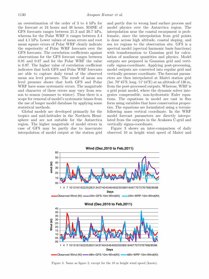
Figure 3 shows an inter-comparison of dailyobserved 10 m height wind speed of Maitri and

00

10

20

30

40

50

60

1 4 7 101316192225283134374043464952555861646770737679828588

win

d (

kt)

Days

Wind (Dec,2010 to Feb,2011)

Observed Wind (Kt) 24hr-GFS-10m-Wind(Kt) 24hr-WRF-10m-Wind(Kt)

00051015202530354045

1 4 7 101316192225283134374043464952555861646770737679828588

Win

d (

kt)

Days

Wind (Dec,2010 to Feb,2011)

Observed Wind (Kt) 48hr-GFS-10m-Wind(Kt) 48hr-WRF-10m-Wind(Kt)

Figure 3. Same as figure 2, except for the 10 m height wind speed (knots).


corresponding interpolated values of 24 hours and48 hours forecasts of 10 m height wind speed fromPolar WRF and IMD GFS for the period from 1December 2010 to 28 February 2011, where strongkatabatic winds are expected. In general, observedpeak values are found to be well-matched with thecorresponding forecast values.

Table 3 presents the performance skill of themodels for 10 m height wind speed forecasts ofMaitri station. GFS shows an overestimation of 1.9knots at 24 hours forecast and an underestimationof 3.8 knots at 48 hours forecast. Whereas PolarWRF shows underestimation of 1.4 knots and 1.3knots at 24 hours and 48 hours forecast. For GFS,RMSE ranges between 10.6 and 8 knots and for thePolar WRF, the values are 5.6 and 4.8 knots. Thecorrelation coefficients of the forecasts against theobserved values are 0.46 and 0.56 for the GFS fore-casts. These values are 0.7 and 0.67 for the PolarWRF forecasts. Superiority of the Polar WRF overthe GFS for 10 m height wind forecasts is clearlyevident form these results.

AMPS is run at 45 km horizontal reso-lution and South Pole is kept at the cen-tre of the model domain. The AMPS graphicoutputs are available in the UCAR web-site http://www.mmm.ucar.edu/rt/amps/. Simi-lar results for AMPS (as in tables 2 and 3)could not be included in this study due to non-accessibility of digital outputs of AMPS. However,graphic products pf AMPS are used in the follow-ing section to compare the forecast flow patternswith that of Polar WRF.

4.2 Validation of forecast flow pattern

The ‘Maitri’ station is located at lat. 70◦45′S,long. 11◦44′E and the model domain is centered at‘Maitri’ with 400 × 400 grid points. Between the60◦ and 65◦S latitudes there exists the Antarctic

Circumpolar Trough, a zone of low pressure thatcontains variable winds flowing from west to east.The importance of this region is that the fiercestorms sweep warm moist air from the middle lati-tudes towards the pole, causing clouds and precip-itation. Storms usually last for a few days, before abrief clearing, then another storm system. In orderto illustrate the performance of Polar WRF, casestudies of two weather events are illustrated in thispaper.

4.2.1 Low pressure system of 8–9 March 2011

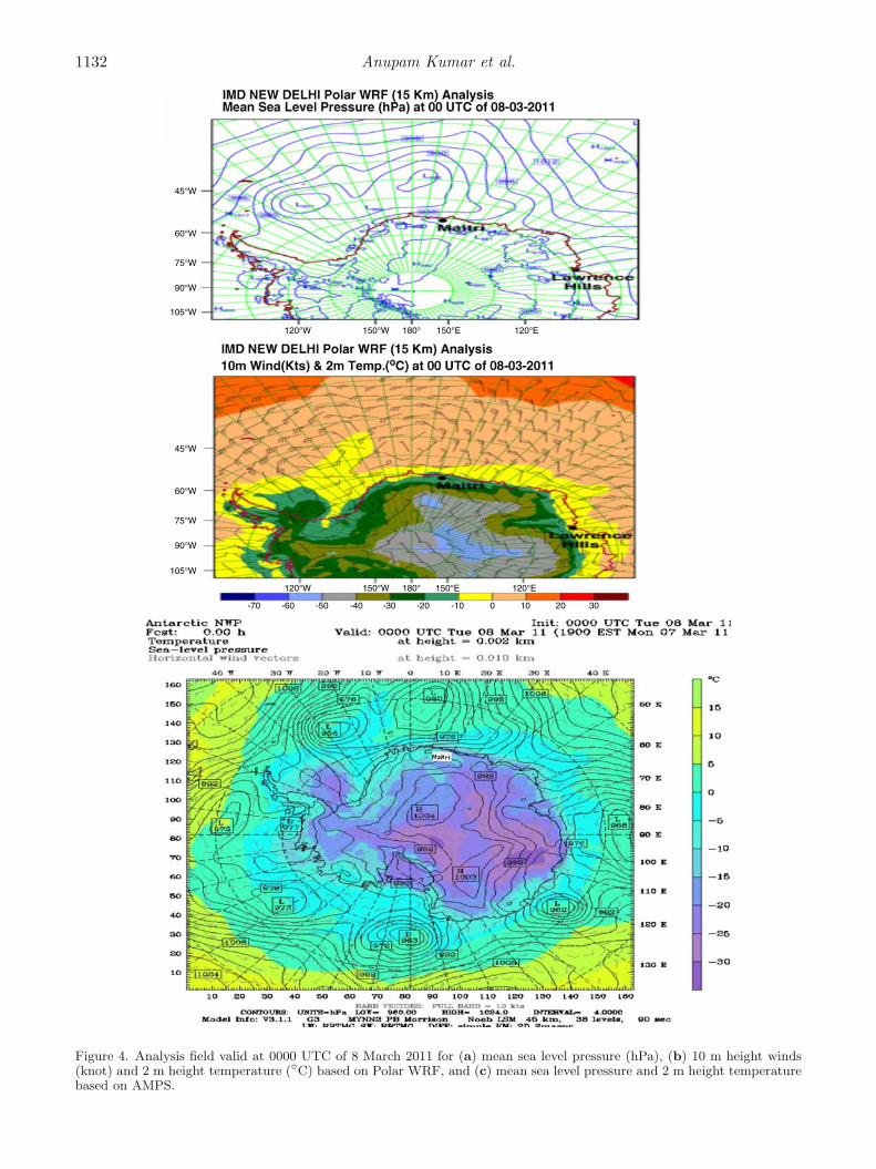
On 8 March 2011, a low pressure area layaround north of Maitri region. Forecast para-meters considered for this exercise are: (a) meansea level pressure and (b) surface (10 m height)wind-superimposed 2 m height temperature. Forcomparison purpose, corresponding analysis andforecast fields of AMPS are used.

Figure 4 displays analysis of mean sea levelpressure field and surface (10 m height) wind-superimposed 2 m height temperature based onPolar WRF and the corresponding AMPS productsvalid at 0000 UTC of 8 March 2011. For the AMPS,the model domain is centred at the Pole, whereasfor the Polar WRF centre of the model centre isat Maitri. The horizontal resolution of AMPS is45 km and the model domain is also different fromthat of Polar WRF.

In the Polar WRF analysis, two low pressureareas are seen to the northwest of Maitri. Two cir-culations in the 10 m height wind field as locatedover this area also justifies the presence of two lowpressure areas. The distribution of 2 m height tem-perature shows −10◦C over Maitri which increasesto the north and becomes 10◦C over the area of lowpressure areas. These features, like two low pres-sure areas to the north-west of Maitri and increaseof 2 m height temperature from −10◦C over Maitri

Table 3. 24 hours and 48 hours forecast skill scores of 10 m height wind speed of Maitri forthe period from 1 December 2010 to 28 February 2011.

Root mean

Mean square Correlation

Wind (kt) errors (kt) errors (kt) coefficient

24 hours

Observation 14.3

GFS 16.1 1.9 10.6 0.46

PWRF 12.8 −1.4 5.6 0.70

48 hours

Observation 14.3

GFS 10.5 −3.8 8.0 0.56

PWRF 13.0 −1.3 4.8 0.67

http://www.mmm.ucar.edu/rt/amps/


45°W

60°W

75°W

90°W

105°W

120°W 120°E150°W 150°E180°

45°W

60°W

75°W

90°W

105°W

120°W 120°E150°W 150°E180°

-70 -60 -50 -40 -30 -20 -10 3020100

Figure 4. Analysis field valid at 0000 UTC of 8 March 2011 for (a) mean sea level pressure (hPa), (b) 10 m height winds(knot) and 2 m height temperature (◦C) based on Polar WRF, and (c) mean sea level pressure and 2 m height temperaturebased on AMPS.


45°W

60°W

75°W

90°W

105°W

120°W 120°E150°W 150°E180°

45°W

60°W

75°W

90°W

105°W

120°W 120°E150°W 150°E180°

-70 -60 -50 -40 -30 -20 -10 3020100

Figure 5. 24 hours forecast field valid at 0000 UTC of 9 March 2011 for (a) mean sea level pressure (hPa), (b) 10 m heightwinds (knot) and 2 m height temperature (◦C) based on Polar WRF, and (c) mean sea level pressure and 2 m heighttemperature based on AMPS.


45°W

60°W

75°W

90°W

105°W

120°W 120°E150°W 150°E180°

45°W

60°W

75°W

90°W

105°W

120°W 120°E150°W 150°E180°

-70 -60 -50 -40 -30 -20 -10 3020100

Figure 6. 48 hours forecast field valid at 0000 UTC of 10 March 2011 for (a) mean sea level pressure (hPa), (b) 10 mheight winds (knot) and 2 m height temperature (◦C) based on Polar WRF, and (c) mean sea level pressure and 2 m heighttemperature based on AMPS.


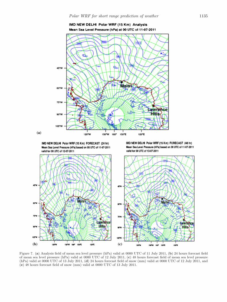
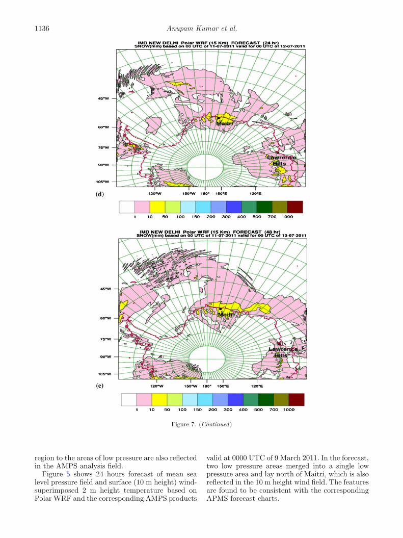
Figure 7. (a) Analysis field of mean sea level pressure (hPa) valid at 0000 UTC of 11 July 2011, (b) 24 hours forecast fieldof mean sea level pressure (hPa) valid at 0000 UTC of 12 July 2011, (c) 48 hours forecast field of mean sea level pressure(hPa) valid at 0000 UTC of 13 July 2011, (d) 24 hours forecast field of snow (mm) valid at 0000 UTC of 12 July 2011, and(e) 48 hours forecast field of snow (mm) valid at 0000 UTC of 13 July 2011.


Figure 7. (Continued)

region to the areas of low pressure are also reflectedin the AMPS analysis field.

Figure 5 shows 24 hours forecast of mean sealevel pressure field and surface (10 m height) wind-superimposed 2 m height temperature based onPolar WRF and the corresponding AMPS products

valid at 0000 UTC of 9 March 2011. In the forecast,two low pressure areas merged into a single lowpressure area and lay north of Maitri, which is alsoreflected in the 10 m height wind field. The featuresare found to be consistent with the correspondingAPMS forecast charts.


Figure 8. (a) Analysis field of mean sea level pressure (hPa) valid at 0000 UTC of 12 July 2011, (b) 24 hours forecast fieldof mean sea level pressure (hPa) valid at 0000 UTC of 13 July 2011, (c) 48 hours forecast field of mean sea level pressure(hPa) valid at 0000 UTC of 14 July 2011, (d) 24 hours forecast field of snow (mm) valid at 0000 UTC of 13 July 2011 and(e) 48 hours forecast field of snow (mm) valid at 0000 UTC of 14 July 2011.

Figure 6 shows 48 hours forecast of mean sealevel pressure field and surface (10 m height) wind-superimposed 2 m height temperature based onPolar WRF and the corresponding AMPS productsvalid at 0000 UTC of 9 March 2011. In the Polar

WRF, the low pressure system moved slightly east-wards and lay just north of Maitri. In the AMPS,the movement of the system to the east is found tobe faster at the 48 hours forecast. Otherwise, boththe forecasts are found to be consistent.


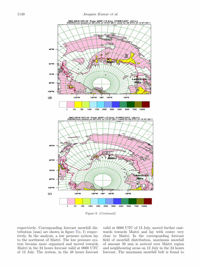
Figure 9. (a) Analysis field of mean sea level pressure (hPa) valid at 0000 UTC of 13 July 2011, (b) 24 hours forecast fieldof mean sea level pressure (hPa) valid at 0000 UTC of 14 July 2011, (c) 48 hours forecast field of mean sea level pressure(hPa) valid at 0000 UTC of 15 July 2011, (d) 24 hours forecast field of snow (mm) valid at 0000 UTC of 14 July 2011, and(e) 48 hours forecast field of snow (mm) valid at 0000 UTC of 15 July 2011.

4.2.2 Low pressure system of 11–14 July 2011

An event of intense blizzard activity was reportedby IMD Maitri station on 13 July 2011 during thepassage of an intense low pressure system. Thiscase is selected to examine the performance of

Polar WRF to capture weather features associatedwith a blizzard activity. Analysis field of mean sealevel pressure (hPa) valid at 0000 UTC of 11 Julyand the 24 hours and 48 hours forecast fields ofmean sea level pressure (hPa) valid at 0000 UTCof 12 and 13 July are shown in figure 7(a, b, c)



respectively. Corresponding forecast snowfall dis-tribution (mm) are shown in figure 7(e, f) respec-tively. In the analysis, a low pressure system layto the northwest of Maitri. The low pressure sys-tem became more organized and moved towardsMaitri in the 24 hours forecast valid at 0000 UTCof 12 July. The system, in the 48 hours forecast

valid at 0000 UTC of 13 July, moved further east-wards towards Maitri and lay with centre veryclose to Maitri. In the corresponding forecastfield of snowfall distribution, maximum snowfallof amount 50 mm is noticed over Maitri regionand neighbouring areas on 12 July in the 24 hoursforecast. The maximum snowfall belt is found to


Figure 10. Analysis field of mean sea level pressure (hPa) valid at 0000 UTC of (a) 14 July 2011 and (b) 15 July 2011.

be extended to eastwards in the corresponding 48hours forecast valid at 0000 UTC of 13 July.

Analysis and forecasts of mean sea level pressuregenerated based on 0000 UTC of 12 July are pre-sented in figure 8(a, b, c). In the analysis of themean sea level pressure, the well marked low pres-sure system is located northwest of Maitri. This isfound to be well captured in the corresponding 24

hours forecast of 11 July (as shown in figure 7b).In the 24 hours forecast valid at 0000 UTC of 13July, the intense low pressure system lay with cen-tre close to Maitri. In the 48 hours forecast validat 0000 UTC of 14 July, the low pressure sys-tem became considerably less marked and lay asan east-west oriented trough line, spreading over alarge area. Corresponding 24 hours forecast field of


snowfall (figure 8d) shows east-west oriented snow-fall belt of intensity 50 mm around Maitri region.In the corresponding 48 hours forecast (figure 8e),the intensity of the snowfall around Maitri regionis found to be less intense.

Analysis and forecasts of mean sea level pressuregenerated based on 0000 UTC of 13 July are pre-sented in figure 9(a, b, c). In the analysis of themean sea level pressure, the organized low pres-sure system is located with centre very close Maitri.This is found to be well captured in the corre-sponding 48 hours forecast of 11 July (as shownin figure 7c) and 24 hours forecast of 12 July (asshown in figure 8b). In the 24 hours forecast validat 0000 UTC of 14 July, the intense low pressuresystem became considerably less marked and layas an east-west oriented trough line, spreading overa large area. This is found to be consistent withthe corresponding 48 hours forecast of 12 July (asshown in figure 8c). Corresponding 24 hours fore-cast field of snowfall (figure 9d) valid at 0000 UTCof 14 July, shows east-west oriented snowfall belt

of intensity 50 mm around Maitri region. In thecorresponding 48 hours forecast (figure 9e) valid at0000 UTC of 15 July, the intensity of the snowfallaround Maitri region is found to be less intense. Infigure 10(a, b), analysis field of mean sea level pres-sure fields (hPa) valid at 0000 UTC of 14 July 2011and 15 July 2011 respectively are presented. Theweakening of the low pressure as reflected in thesefigures, is clearly captured in the correspondingforecasts generated on 12 and 13 July.

Figure 11 presents Meteogram of Maitri for 48hours forecast issued at 0000 UTC of 13 July 2011.Strong westerly winds of order around 100 knotsare noticed in the hourly forecasts during morning0000 UTC of 13 July to 0000 UTC of 14 July. Windspeed in the forecast started decreasing after 0000UTC of 14 July and became 40 knots at 1200 UTCof 14 July. According to the observations receivedfrom Maitri station, wind speed has been 69 knots,gusting to 96 knots during 13 July. Thus, the modelis able to provide realistic wind forecasts of thisblizzard event. In the forecast, snowfall is observed

Figure 11. Meteogram of Maitri for 48 hours forecast issued at 0000 UTC of 13 July 2011.


during early forecast hours up to 0800 UTC. Sur-face humidity in the forecast has been around 80%during 0000 UTC 13 July to 1200 UTC of 14 Julyand then started decreasing. It became 40% at 0000UTC of 15 July, in the 48 hours forecast. Surfacetemperature has been around −8◦C at 0000 UTCof 13 July to 0000 UTC 14 July, and then starteddecreasing. It became −15◦C at 0000 UTC of 15July, after the ceasing of the blizzard event on 14July. Mean sea level pressure started decreasingfrom 972 hPa at 0000 UTC of 13 July and became966 hPa at 1800 UTC of 13 July. Thereafter againit started increasing and became 972 at 0000 UTCof 15 July. These results are found to be well com-parable with the reports received from the Maitristation.

5. Conclusions

To meet the operational need of weather forecastsfor Maitri region, recently Polar WRF at 15 kmhorizontal resolution is made operational at IMDNew Delhi using IMD GFS T-382 as the initialand boundary conditions (the current operationalversion of the model is GFS T574). Location spe-cific short range forecasts generated interpolatingPolar WRF outputs are compared with the cor-responding observed fields of Maitri and forecastfields of IMD GFS using data for the period of90 days starting from 1 December 2010 to 28 Febru-ary 2011. The time series of observed and corre-sponding forecast fields shown in this comparisonindicates a high level of agreement of Polar WRFwith the observed field. The performance statistics,such as mean errors, root mean square errors andcorrelation coefficient of forecasts of mean sea levelpressure and 10 m height wind computed againstthe corresponding observations of Maitri clearlydemonstrated the superiority of Polar WRF fore-casts over the IMD GFS forecasts. The case studiespresented in this paper clearly demonstrated thepotential of the model to capture frontal low pres-sure systems and associated weather features. Thestudy demonstrates the usefulness of the forecastproducts for short range forecasting of weather overthe Maitri region.

However, these results being preliminary, fur-ther investigation is needed for a variety of differ-ent weather conditions during winter and summermonths for identifying shortcomings of the modeland aspects of the model that require additionaldevelopment work in the future.

Acknowledgements

Authors are grateful to the Director Generalof Meteorology, India Meteorological Department,New Delhi for his keen interest in this study andproviding all facilities and support to complete thework. Authors thankfully acknowledge the Meteo-rology Group of the Byrd Polar Research Centerat the Ohio State University for use of the PolarWRF in this work and technical guidance throughe-mail interactions.

References

Bromwich D H, Cassano J J, Klein T, Hrinemann G, HinesK M, Steffen K and Box J E 2001 Meso-scale modeling ofkatabatic winds over Greenland with Polar MM5; Mon.Weather Rev. 129 2290–2309.

Cassano J J and Parish T R 2000 An analysis of the non-hydrostatic dynamics in numerically simulated Antarctickatabatic flows; J. Atmos. Sci. 57 891–898.

Cassano J J, Parish T R and King J C 2001a Evaluationof turbulent surface flux parameterizations for the stablesurface layer over Halley, Antarctica; Mon. Weather Rev.129 26–46.

Cassano J J, Box J E, Bromwich D H, Li L and Stef-fen K 2001b Evaluation of Polar MM5 simulations ofGreenland’s atmospheric circulation; J. Geophys. Res.106 33,867–33,890.

Hines K M and Bromwich D H 2008 Development and test-ing of Polar WRF. Part I. Greenland ice sheet meteorol-ogy; Mon. Weather Rev. 136 1971–1989.

Pandey P C 2007 “India: Antarctic Program”, Encyclope-dia of the Antarctic (ed.) Beau Riffenburgh, Abingdonand New York: Taylor & Francis, ISBN 0–415–97024–5,pp. 529–530.

Parish T R and Cassano J J 2003 Diagnosis of the katabaticwind influence on the wintertime Antarctic surface windfield from numerical simulations; Mon. Weather Rev. 1311128–1139.

Pavolonis M J, Key J R and Cassano J J 2004 A study ofthe Antarctic surface energy budget using a polar regionalatmospheric model forced with satellite derived cloudproperties; Mon. Weather Rev. 132 654–661.

Powers J G 2007 Numerical prediction of an Antarctic severewind event with the weather research and forecasting(WRF) model; Mon. Weather Rev. 135 3134–3157.

Powers J G, Monaghan A J, Cayette A M, Bromwich D H,Kuo Y–H and Manning K W 2003 Real time mesoscalemodeling over Antarctica: The Antarctica Meso-scalePrediction System (AMPS); Bull. Am. Meteor. Soc. 841533–1545.

Roy Bhowmik S K and Durai V R 2010 “Performance ofGlobal Forecast System of IMD in the medium range timescale during summer monsoon 2010” – Monsoon 2010, Areport of IMD, Met Mongraph Synoptic Meteorology No.10/2011, pp. 101–132.

Schwedtfeger W 1984 Weather and Climate of Antartic;Elsevier, 261p.

MS received 14 January 2012; revised 3 May 2012; accepted 8 May 2012

implementation of polar wrf for short range prediction of

Documents