implementations of fourier methods in cfd to analyze

Brigham Young UniversityBYU ScholarsArchive

All Theses and Dissertations

2016-06-01

Implementations of Fourier Methods in CFD toAnalyze Distortion Transfer and GenerationThrough a Transonic FanMarshall Warren PetersonBrigham Young University

Follow this and additional works at: https://scholarsarchive.byu.edu/etd

Part of the Mechanical Engineering Commons

This Thesis is brought to you for free and open access by BYU ScholarsArchive. It has been accepted for inclusion in All Theses and Dissertations by anauthorized administrator of BYU ScholarsArchive. For more information, please contact [email protected], [email protected].

BYU ScholarsArchive CitationPeterson, Marshall Warren, "Implementations of Fourier Methods in CFD to Analyze Distortion Transfer and Generation Through aTransonic Fan" (2016). All Theses and Dissertations. 6384.https://scholarsarchive.byu.edu/etd/6384

http://home.byu.edu/home/?utm_source=scholarsarchive.byu.edu%2Fetd%2F6384&utm_medium=PDF&utm_campaign=PDFCoverPages

http://home.byu.edu/home/?utm_source=scholarsarchive.byu.edu%2Fetd%2F6384&utm_medium=PDF&utm_campaign=PDFCoverPages

https://scholarsarchive.byu.edu?utm_source=scholarsarchive.byu.edu%2Fetd%2F6384&utm_medium=PDF&utm_campaign=PDFCoverPages

https://scholarsarchive.byu.edu/etd?utm_source=scholarsarchive.byu.edu%2Fetd%2F6384&utm_medium=PDF&utm_campaign=PDFCoverPages

https://scholarsarchive.byu.edu/etd?utm_source=scholarsarchive.byu.edu%2Fetd%2F6384&utm_medium=PDF&utm_campaign=PDFCoverPages

http://network.bepress.com/hgg/discipline/293?utm_source=scholarsarchive.byu.edu%2Fetd%2F6384&utm_medium=PDF&utm_campaign=PDFCoverPages

https://scholarsarchive.byu.edu/etd/6384?utm_source=scholarsarchive.byu.edu%2Fetd%2F6384&utm_medium=PDF&utm_campaign=PDFCoverPages

mailto:[email protected],%[email protected]

Implementations of Fourier Methods in CFD to Analyze Distortion Transfer and Generation

Through a Transonic Fan

Marshall Warren Peterson

A thesis submitted to the faculty ofBrigham Young University

in partial fulfillment of the requirements for the degree of

Master of Science

Steven E. Gorrell, ChairJerry BowmanJulie Crockett

Department of Mechanical Engineering

Brigham Young University

June 2016

Copyright © 2016 Marshall Warren Peterson

All Rights Reserved

ABSTRACT

Implementations of Fourier Methods in CFD to Analyze Distortion Transfer and GenerationThrough a Transonic Fan

Marshall Warren PetersonDepartment of Mechanical Engineering, BYU

Master of Science

Inlet flow distortion is a non-uniform total pressure, total temperature, or swirl (flow angu-larity) condition at an aircraft engine inlet. Inlet distortion is a critical consideration in modern fanand compressor design. This is especially true as the industry continues to increase the efficiencyand operating range of air breathing gas turbine engines. The focus of this paper is to evaluatethe Computational Fluid Dynamics (CFD) Harmonic Balance (HB) solver in STAR-CCM+ as areduced order method for capturing inlet distortion as well as the associated distortion transfer andgeneration. New methods for quantitatively describing and analyzing distortion transfer and gen-eration are investigated. The geometry used is the rotor 4 fan geometry, consisting of one rotor andone stator. The inlet boundary condition is a 90◦ sector total pressure distortion profile with totalpressure and swirl held constant.

Multiple HB simulations with varying mode combinations and distortion intensities are an-alyzed and compared against full annulus Unsteady Reynolds Averaged Navier-Stokes (URANS)simulations. Best practices and recommendations for the implementation of the HB solver aregiven.

The pre-existing Society of Automotive Engineers Aerospace Recommended Practice (SAE-ARP) 1420b descriptors are demonstrated to be inadequate for the purposes of analyzing distortiontransfer and generation on a stage-to-stage basis. New implementations of Fourier methods are pre-sented as an alternative to the SAE-ARP 1420b descriptors. These Fourier descriptors are shown todescribe distortion transfer and generation to a higher degree of fidelity than the SAE-ARP 1420bdescriptors. These new descriptors are demonstrated on the analysis of full annulus URANS andHB simulations. The HB solver is shown to be capable of capturing distortion transfer, genera-tion and performance degradation. Recommendations for the optimal implementation of the HBmethod are given.

Keywords: turbomachinery, Fourier, Fourier analysis, harmonic balance, computational fluid dy-namics, CFD, SAE-ARP 1420b, distortion, inlet distortion, distortion transfer, distortion genera-tion, rotor 4, AFRL

ACKNOWLEDGMENTS

I express my utmost appreciation to my graduate advisor, Dr. Steven E. Gorrell, for guiding,

assisting and mentoring me through this research endeavor. I am grateful for his guidance and

expertise which was pivotal to the success of this project. His positive and consistent feedback and

direction was much appreciated. I’m also grateful for his support in allowing me to explore and

pursue my own ideas and solutions.

I would also like to express my gratitude to the remainder of my committee, Dr. W. Jerry

Bowman and Dr. Julie Crockett. I am also grateful for the world-class peers that I had the priv-

ilege of working along side of in the BYU Turbomachinery Research Lab. Their collaboration

and advice was always welcome. I am also appreciative of the BYU Mechanical Engineering

Department, which contains some of the best professors and administrative staff in the world.

I gratefully acknowledge the funding provided by the United States Air Force under Con-

tract No. PP-CFD-KY06-010-P3 that made this research possible. I would like to personally thank

Dr. Michael List of the Air Force Research Lab for his guidance, support and expertise.

Finally, I would like to thank my loving wife, Emily Peterson, for her constant support. I

could not have made it to this point without her.

TABLE OF CONTENTS

LIST OF TABLES . . . . . . . . . . . . . . . . . . . . . . . . . . . . . . . . . . . . . . . vi

LIST OF FIGURES . . . . . . . . . . . . . . . . . . . . . . . . . . . . . . . . . . . . . . vii

NOMENCLATURE . . . . . . . . . . . . . . . . . . . . . . . . . . . . . . . . . . . . . . x

Chapter 1 Introduction . . . . . . . . . . . . . . . . . . . . . . . . . . . . . . . . . . . 1

Chapter 2 Background and Literature Review . . . . . . . . . . . . . . . . . . . . . . 42.1 Diffuser Physics . . . . . . . . . . . . . . . . . . . . . . . . . . . . . . . . . . . . 42.2 Distortion Handling . . . . . . . . . . . . . . . . . . . . . . . . . . . . . . . . . . 5

2.2.1 Distortion Descriptors . . . . . . . . . . . . . . . . . . . . . . . . . . . . 62.2.2 Select Analytical and Experimental Efforts . . . . . . . . . . . . . . . . . 8

2.3 CFD . . . . . . . . . . . . . . . . . . . . . . . . . . . . . . . . . . . . . . . . . . 92.3.1 CFD Methods . . . . . . . . . . . . . . . . . . . . . . . . . . . . . . . . . 92.3.2 CFD Efforts Applied to Distortion . . . . . . . . . . . . . . . . . . . . . . 13

Chapter 3 Fan and Distortion Profile Selection . . . . . . . . . . . . . . . . . . . . . 153.1 Geometry . . . . . . . . . . . . . . . . . . . . . . . . . . . . . . . . . . . . . . . 153.2 Distortion Profiles . . . . . . . . . . . . . . . . . . . . . . . . . . . . . . . . . . . 16

Chapter 4 Methodology . . . . . . . . . . . . . . . . . . . . . . . . . . . . . . . . . . 214.1 Turbomachinery Mesh Generation Best Practices . . . . . . . . . . . . . . . . . . 21

4.1.1 Mesh Quality . . . . . . . . . . . . . . . . . . . . . . . . . . . . . . . . . 224.1.2 Mesh Recommendations . . . . . . . . . . . . . . . . . . . . . . . . . . . 254.1.3 Mesh Troubleshooting . . . . . . . . . . . . . . . . . . . . . . . . . . . . 28

4.2 Initial Steady State Solution . . . . . . . . . . . . . . . . . . . . . . . . . . . . . 304.3 Full Annulus URANS . . . . . . . . . . . . . . . . . . . . . . . . . . . . . . . . . 32

4.3.1 Full Annulus Process . . . . . . . . . . . . . . . . . . . . . . . . . . . . . 324.4 Harmonic Balance . . . . . . . . . . . . . . . . . . . . . . . . . . . . . . . . . . 33

4.4.1 Blade Rows . . . . . . . . . . . . . . . . . . . . . . . . . . . . . . . . . . 334.4.2 Modes . . . . . . . . . . . . . . . . . . . . . . . . . . . . . . . . . . . . . 334.4.3 Wake Specification . . . . . . . . . . . . . . . . . . . . . . . . . . . . . . 344.4.4 Time Levels . . . . . . . . . . . . . . . . . . . . . . . . . . . . . . . . . . 374.4.5 Harmonic Balance Simulations . . . . . . . . . . . . . . . . . . . . . . . . 394.4.6 Harmonic Balance Process . . . . . . . . . . . . . . . . . . . . . . . . . . 39

4.5 Post Processing . . . . . . . . . . . . . . . . . . . . . . . . . . . . . . . . . . . . 394.5.1 Time Averaging . . . . . . . . . . . . . . . . . . . . . . . . . . . . . . . . 404.5.2 Mass Flow Time Averaging . . . . . . . . . . . . . . . . . . . . . . . . . 404.5.3 Tradition Distortion Descriptors . . . . . . . . . . . . . . . . . . . . . . . 424.5.4 Fourier Analysis . . . . . . . . . . . . . . . . . . . . . . . . . . . . . . . 43

iv

Chapter 5 Results . . . . . . . . . . . . . . . . . . . . . . . . . . . . . . . . . . . . . . 475.1 Evaluation of Distortion Descriptors . . . . . . . . . . . . . . . . . . . . . . . . . 47

5.1.1 SAE-ARP 1420-b Descriptors . . . . . . . . . . . . . . . . . . . . . . . . 495.1.2 Fourier Analysis for Describing Distortion . . . . . . . . . . . . . . . . . 545.1.3 Discussion of Distortion Descriptor Results . . . . . . . . . . . . . . . . . 62

5.2 Full Annulus URANS Results . . . . . . . . . . . . . . . . . . . . . . . . . . . . 645.2.1 Qualitative 7.5% Full Annulus URANS . . . . . . . . . . . . . . . . . . . 655.2.2 15% Full Annulus URANS . . . . . . . . . . . . . . . . . . . . . . . . . . 715.2.3 Quantitative Distortion Transfer and Generation Comparison . . . . . . . . 765.2.4 Performance Parameters . . . . . . . . . . . . . . . . . . . . . . . . . . . 845.2.5 Discussion of 7.5% and 15% Distortion Comparison Results . . . . . . . . 86

5.3 Harmonic Balance Results . . . . . . . . . . . . . . . . . . . . . . . . . . . . . . 875.3.1 Computational Cost Comparison . . . . . . . . . . . . . . . . . . . . . . . 875.3.2 Distortion Transfer and Generation Comparison . . . . . . . . . . . . . . . 895.3.3 Fan Performance Comparison . . . . . . . . . . . . . . . . . . . . . . . . 995.3.4 Discussion of Harmonic Balance Results . . . . . . . . . . . . . . . . . . 101

Chapter 6 Conclusions . . . . . . . . . . . . . . . . . . . . . . . . . . . . . . . . . . . 1036.1 Future Work . . . . . . . . . . . . . . . . . . . . . . . . . . . . . . . . . . . . . . 105

REFERENCES . . . . . . . . . . . . . . . . . . . . . . . . . . . . . . . . . . . . . . . . . 108

Appendix A Supplementary Processes . . . . . . . . . . . . . . . . . . . . . . . . . . . 110A.1 STAR-CCM+ Mesh Processes . . . . . . . . . . . . . . . . . . . . . . . . . . . . 110

A.1.1 Refining Leading and Trailing Edges . . . . . . . . . . . . . . . . . . . . 110A.1.2 Setting Up Prism Layer Mesh . . . . . . . . . . . . . . . . . . . . . . . . 111A.1.3 Checking for Conformal Interfaces . . . . . . . . . . . . . . . . . . . . . 112A.1.4 Adjusting Boundary March Angle . . . . . . . . . . . . . . . . . . . . . . 112

A.2 Initial Steady State Solution Process . . . . . . . . . . . . . . . . . . . . . . . . . 113A.3 Full Annulus URANS Solution Process . . . . . . . . . . . . . . . . . . . . . . . 116A.4 Harmonic Balance Solution Process . . . . . . . . . . . . . . . . . . . . . . . . . 118A.5 Harmonic Balance 15% Distortion Attempts . . . . . . . . . . . . . . . . . . . . . 121

A.5.1 Full Annulus Inlet Method . . . . . . . . . . . . . . . . . . . . . . . . . . 121A.5.2 Wake Specification Method . . . . . . . . . . . . . . . . . . . . . . . . . 122

A.6 Full Annulus Time Averaging Process . . . . . . . . . . . . . . . . . . . . . . . . 123

Appendix B Supplementary Results . . . . . . . . . . . . . . . . . . . . . . . . . . . . . 124

v

LIST OF TABLES

3.1 Rotor 4 design parameters. . . . . . . . . . . . . . . . . . . . . . . . . . . . . . . 16

4.1 Mesh quality metric recommendations . . . . . . . . . . . . . . . . . . . . . . . . 254.2 Mixing-plane mesh cell count (single rotor and single stator passage). . . . . . . . 314.3 Full annulus mesh cell counts (1 spinner, 20 rotor and 31 stators). . . . . . . . . . 324.4 Time levels for a (2-0) simulation. . . . . . . . . . . . . . . . . . . . . . . . . . . 374.5 Time levels for a (2-1) simulation. . . . . . . . . . . . . . . . . . . . . . . . . . . 384.6 Fourier modal descriptors for the 15% total pressure distortion profile at 50% span. 45

5.1 Fourier total amplitude descriptor applied to distortion transfer and generation forthe time averaged 15% full annulus URANS data at 50% span. . . . . . . . . . . . 62

5.2 Total amplitude of distortion transfer and generation for the radial and time-averaged7.5% and 15% full annulus data. . . . . . . . . . . . . . . . . . . . . . . . . . . . 79

5.3 Comparison of the fan performance values for the 7.5% and 15% full annulusURANS simulaions. . . . . . . . . . . . . . . . . . . . . . . . . . . . . . . . . . 85

5.4 Comparison of the convergence computational cost requirements for the 7.5% fullannulus URANS simulation and the HB simulations. . . . . . . . . . . . . . . . . 88

5.5 Total amplitude of distortion transfer and generation for the radial and time-averagedHB(5-0-0) and 7.5% full annulus data. . . . . . . . . . . . . . . . . . . . . . . . . 92



5.8 Comparison of the fan performance values for the 7.5% full annulus URANS sim-ulation and the HB simulations. . . . . . . . . . . . . . . . . . . . . . . . . . . . . 100

B.1 Distortion transfer and generation Fourier descriptors for the time averaged 7.5%full annulus URANS data. . . . . . . . . . . . . . . . . . . . . . . . . . . . . . . 130

B.2 Distortion transfer and generation Fourier descriptors for the radial and time aver-aged 7.5% full annulus URANS data. . . . . . . . . . . . . . . . . . . . . . . . . 131

B.3 Distortion transfer and generation Fourier descriptors for the time averaged 15%full annulus URANS data. . . . . . . . . . . . . . . . . . . . . . . . . . . . . . . 132

B.4 Distortion transfer and generation Fourier descriptors for the radial and time aver-aged 15% full annulus URANS data. . . . . . . . . . . . . . . . . . . . . . . . . . 133

vi

LIST OF FIGURES

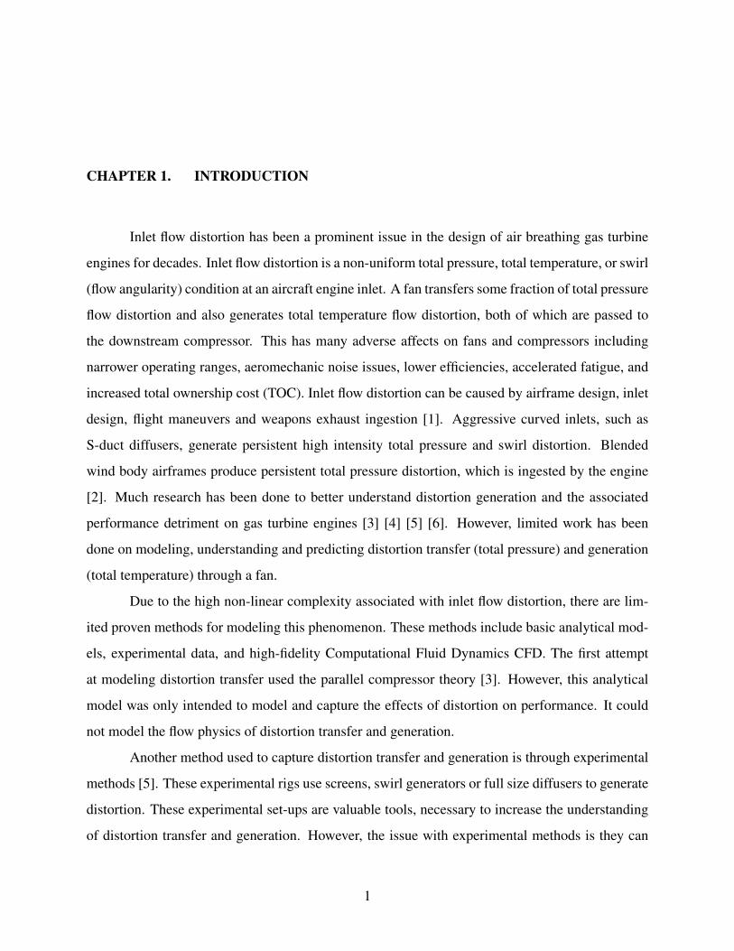
2.1 Normalized distortion generated in an S-duct diffuser. Flow direction is right toleft. Red green and blue in the color map are equal to 1, 0 and -1 respectively. . . . 5

2.2 SAE-ARP 1420b ring circumferential distortion [8]. . . . . . . . . . . . . . . . . . 72.3 Representations of an inlet distortion profile using the full annulus URANS, mixing-

plane, periodic and HB methods. . . . . . . . . . . . . . . . . . . . . . . . . . . . 102.4 CFD and experimental comparison of total pressure and total temperature profiles

at 50% immersion. Lines with rapid oscillation are the time instantaneous CFDsolution. Overlaid smoother lines are the time-averaged CFD solution. Solid sym-bols are experimental data [6]. . . . . . . . . . . . . . . . . . . . . . . . . . . . . 13

3.1 Air Force Research Lab rotor 4 geometry. . . . . . . . . . . . . . . . . . . . . . . 163.2 Total pressure distortion profiles used. . . . . . . . . . . . . . . . . . . . . . . . . 173.3 Total pressure harmonic content present in the 15% 90◦ sector distortion profile at

the rotor inlet. . . . . . . . . . . . . . . . . . . . . . . . . . . . . . . . . . . . . . 193.4 180◦ 1-per-rev inlet distortion profile compared with the 1 mode Fourier series

representation. . . . . . . . . . . . . . . . . . . . . . . . . . . . . . . . . . . . . . 19

4.1 Mesh quality metrics [22]. . . . . . . . . . . . . . . . . . . . . . . . . . . . . . . 224.2 Mesh quality metrics continued [22]. . . . . . . . . . . . . . . . . . . . . . . . . . 234.3 High resolution rotor 4 blade leading edge surface mesh. . . . . . . . . . . . . . . 264.4 Rotor 4 blade tip gap volume mesh. . . . . . . . . . . . . . . . . . . . . . . . . . 274.5 Rotor 4 high resolution prism layer volume mesh. . . . . . . . . . . . . . . . . . . 284.6 Non-uniform prism layer observed in preliminary mesh. . . . . . . . . . . . . . . 304.7 Single passage computational domains (a) with spinner region and (b) without. . . 314.8 Example of the effect of modes in the rotor blade row on the solution. . . . . . . . 354.9 Circumferential average of a) gauge total pressure and b) absolute total temperature

used for the wake specification for all HB simulations. . . . . . . . . . . . . . . . 364.10 Circumferential variation in a) static pressure, b) static temperature and c) axial

velocity used for the wake specification for all HB simulations. . . . . . . . . . . . 364.11 HB Solution view representation of HB 5-0-0 at a constant radius of 0.175m (75%

span of the rotor leading edge). . . . . . . . . . . . . . . . . . . . . . . . . . . . . 414.12 15% total pressure distortion at 50% span with SAE-ARP 1420-b values reported. . 424.13 Fourier modes of the 15% total pressure distortion profile at 50% span. . . . . . . . 444.14 Fourier modal amplitude for the 15% total pressure distortion profile at 50% span

for the rotor inlet, stator inlet and stator outlet. . . . . . . . . . . . . . . . . . . . . 45

5.1 SAE-ARP descriptors applied to distortion transfer for the time averaged 15% fullannulus URANS data at 50% span for the rotor inlet, stator inlet and stator outletprofiles. . . . . . . . . . . . . . . . . . . . . . . . . . . . . . . . . . . . . . . . . 50

5.2 SAE-ARP descriptors applied to distortion generation for the time averaged 15%full annulus URANS data at 50% span for the rotor inlet, stator inlet and statoroutlet profiles. . . . . . . . . . . . . . . . . . . . . . . . . . . . . . . . . . . . . . 51

vii

5.3 Fourier descriptors applied to distortion transfer for the time averaged 15% fullannulus URANS data at 50% span for the rotor inlet, stator inlet and stator outletprofiles. . . . . . . . . . . . . . . . . . . . . . . . . . . . . . . . . . . . . . . . . 55

5.4 Fourier descriptors applied to distortion generation for the time averaged 15% fullannulus URANS data at 50% span for the rotor inlet, stator inlet and stator outletprofiles. . . . . . . . . . . . . . . . . . . . . . . . . . . . . . . . . . . . . . . . . 56

5.5 Fourier modal amplitudes applied to distortion transfer and generation for the timeaveraged 15% full annulus URANS data at 50% span for the rotor inlet, stator inletand stator outlet profiles. . . . . . . . . . . . . . . . . . . . . . . . . . . . . . . . 57

5.6 Example periodic profiles with varying modal amplitudes and fixed modal phase . 595.7 Plots a) and b) show the comparison of modal amplitudes. Plot c) shows the total

amplitudes of all 3 profiles. . . . . . . . . . . . . . . . . . . . . . . . . . . . . . . 595.8 Axial profile map used for referencing circumferential and radial locations. . . . . 665.9 Time averaged 7.5% full annulus URANS data. . . . . . . . . . . . . . . . . . . . 675.10 Time averaged 15% full annulus URANS data. . . . . . . . . . . . . . . . . . . . 725.11 Comparison of the radial-averaged distortion transfer and generation for the 7.5%

and 15% full annulus URANS data. . . . . . . . . . . . . . . . . . . . . . . . . . 775.12 Fourier modal amplitudes applied to distortion transfer and generation for the ra-

dial and time-averaged 7.5% full annulus URANS data for the rotor inlet, statorinlet and stator outlet. . . . . . . . . . . . . . . . . . . . . . . . . . . . . . . . . . 78

5.13 Fourier modal amplitudes applied to distortion transfer and generation for the ra-dial and time-averaged 15% full annulus URANS data for the rotor inlet, statorinlet and stator outlet. . . . . . . . . . . . . . . . . . . . . . . . . . . . . . . . . . 78

5.14 Comparison of the radial time-averaged total pressure and total temperature pro-files at the rotor inlet, stator inlet and stator outlet for the HB(5-0-0) and 7.5% fullannulus data. . . . . . . . . . . . . . . . . . . . . . . . . . . . . . . . . . . . . . 90

5.15 Comparison of the radial time-averaged total pressure and total temperature modalamplitudes at the rotor inlet, stator inlet and stator outlet for the HB(5-0-0) and7.5% full annulus data. . . . . . . . . . . . . . . . . . . . . . . . . . . . . . . . . 91





B.1 Comparison of distortion transfer and generation for the time averaged 7.5% fullannulus URANS data. . . . . . . . . . . . . . . . . . . . . . . . . . . . . . . . . . 125

viii

B.2 Comparison of distortion transfer and generation for the time averaged 15% fullannulus URANS data. . . . . . . . . . . . . . . . . . . . . . . . . . . . . . . . . . 126

B.3 Modal visualization of distortion transfer and generation for the time averaged7.5% full annulus URANS data. . . . . . . . . . . . . . . . . . . . . . . . . . . . 127

B.4 Modal visualization of distortion transfer and generation for the time averaged 15%full annulus URANS data. . . . . . . . . . . . . . . . . . . . . . . . . . . . . . . 128

B.5 Distortion transfer and generation for the time averaged 7.5% and 15% full annulusURANS data. . . . . . . . . . . . . . . . . . . . . . . . . . . . . . . . . . . . . . 129

ix

NOMENCLATURE

~a Normal of a cell faceA Fourier modal amplitudeBR Number of blade rows∆φ Change in Fourier modal phase~ds Vector between two adjacent cell centroidsη f Fan polytropic efficiencyγ Isentropic expansion factorI Total pressure distortion intensityM Number of non-reflecting modesn n-th mode of the Fourier series expansionN Total number of Fourier modesNe f f ective Effective mesh cell countNi Number of cells

i-th blade rowNmin Minimum number of cells required to prevent aliasingp Fundamental period of a repeating profileP Static or thermodynamic pressurePt Total or stagnation pressurePAV Circumferential-average of the total pressurePAV LOW Circumferential-average of the low total pressureφ Fourier modal phaseπ f Fan total pressure ratioPk−Pk Peak-to-peak amplitudeQ Number of low-pressure regions in a distortion profile (per-rev components)ΣA Total Fourier amplitudeT Static or thermodynamic temperatureTt Total or stagnation temperatureτ f Fan total temperature ratioθi Total pressure distortion extent

i-th ring of the profileT L Number of time levelsy+ y-plus value

x

CHAPTER 1. INTRODUCTION

Inlet flow distortion has been a prominent issue in the design of air breathing gas turbine

engines for decades. Inlet flow distortion is a non-uniform total pressure, total temperature, or swirl

(flow angularity) condition at an aircraft engine inlet. A fan transfers some fraction of total pressure

flow distortion and also generates total temperature flow distortion, both of which are passed to

the downstream compressor. This has many adverse affects on fans and compressors including

narrower operating ranges, aeromechanic noise issues, lower efficiencies, accelerated fatigue, and

increased total ownership cost (TOC). Inlet flow distortion can be caused by airframe design, inlet

design, flight maneuvers and weapons exhaust ingestion [1]. Aggressive curved inlets, such as

S-duct diffusers, generate persistent high intensity total pressure and swirl distortion. Blended

wind body airframes produce persistent total pressure distortion, which is ingested by the engine

[2]. Much research has been done to better understand distortion generation and the associated

performance detriment on gas turbine engines [3] [4] [5] [6]. However, limited work has been

done on modeling, understanding and predicting distortion transfer (total pressure) and generation

(total temperature) through a fan.

Due to the high non-linear complexity associated with inlet flow distortion, there are lim-

ited proven methods for modeling this phenomenon. These methods include basic analytical mod-

els, experimental data, and high-fidelity Computational Fluid Dynamics CFD. The first attempt

at modeling distortion transfer used the parallel compressor theory [3]. However, this analytical

model was only intended to model and capture the effects of distortion on performance. It could

not model the flow physics of distortion transfer and generation.

Another method used to capture distortion transfer and generation is through experimental

methods [5]. These experimental rigs use screens, swirl generators or full size diffusers to generate

distortion. These experimental set-ups are valuable tools, necessary to increase the understanding

of distortion transfer and generation. However, the issue with experimental methods is they can

1

take years from conception to final data analysis and can cost millions of dollars. Another issue

is there are limited parameters that can be measured, and limited engine locations where such

measurements can be taken. Also most of the probes used are invasive, altering the true flow.

These rigs also require a large amount of space, specialized equipment and facilities, and a team

of engineers and technicians to operate and maintain.

A promising alternative to experimental and analytical approaches is to leverage high per-

formance computing using high-fidelity CFD. CFD removes the need for large, expensive experi-

mental rigs. CFD is also not limited in what parameters can be measured and where. Full annulus

Unsteady Reynolds-Averaged Navier-Stokes (URANS) simulations have been shown to capture

distortion transfer and generation with reasonable accuracy [6]. However, the issue with these

simulations is that they can require hundreds of millions of cells, requiring weeks to solve on

thousands of processors and producing terabytes of data. Such factors limit the number of design

iterations that can be accomplished in a timely manner.

The Harmonic Balance (HB) solver is an alternative to the full annulus URANS solver, that

if proven to capture distortion transfer and generation with relative accuracy, could be a valuable

tool for modeling this phenomenon. The HB solver uses Fourier methods to truncate the full

annulus domain while still capturing full annulus information. Fourier methods use of the sum

of trigonometric functions to approximate any periodic profile. The sum of these trigonometric

functions is known as the Fourier series. Fourier methods have been implemented in many fields

for a wide range of applications and are a time tested, proven method for capturing and analyzing

periodic behavior [7]. The reduction in computational domain achieved by the implementation

of Fourier methods translates to faster convergence times and lower resource requirements. This

allows for more design iterations in a given time frame than the full annulus URANS solver can

achieve.

Fourier methods can also be applied to post-processing to quantify distortion transfer and

generation. Quantifying these phenomena is important in order to increase understanding and to be

able to produce more accurate predictive analytical and numerical models. Current methods only

capture specific types of distortion and do not account for the reshaping of distortion profiles. The

Fourier series has been shown to capture any type of periodic profile. Therefore the Fourier series

2

coefficients may be able to describe the magnitude, and shape of any given distortion profile. This

results in robust descriptors that may be applied to any given distortion parameter at any location.

There are three main objectives of this thesis. These are as follows:

1. Investigate the application of Fourier methods to capture distortion transfer and generation.

The Fourier descriptors are compared against the industry standard Society of Automotive

Engineers, Aerospace Recommended Practice (SAE-ARP) 1420b [8] descriptors on multiple

data sets to evaluate their ability to quantitatively describe distortion phenomenons. The

significance of this evaluation is it provides a new set of quantitative descriptors that set the

foundation for more robust analytical and numerical models. These descriptors also aid to

increase current understanding of distortion phenomenon.

2. Provide best practices and recommendations for applying the HB solver in STAR-CCM+ to

capture total pressure distortion transfer and total temperature distortion generation. This

thesis is the first to implement the HB solver for this purpose. Therefore, much work was

required to successfully converge the HB solver. The process followed is meticulously doc-

umented in this report.

3. Evaluate the ability of the HB solver in STAR-CCM+ to capture total pressure distortion

transfer, total temperature distortion generation and fan performance. The computational

requirements to achieve a converged solution are also evaluated. The significance of this

evaluation is it assesses the potential value of the HB solver for use in both design and

research applications for fans/compressors with inlet distortion present.

The paper will proceed as follows: background and literature review including impact of

inlet distortion, methods for modeling distortion, and the fundamentals of the HB solver; simula-

tion set up including selected geometry and distortion profiles; methodology including mesh best

practices, initial solution, full annulus URANS, HB and post-processing; final results including

Fourier analysis, full annulus URANS comparison and HB comparison; conclusions.

3

CHAPTER 2. BACKGROUND AND LITERATURE REVIEW

This chapter discusses the background and motivation of the current thesis. This is done

by discussing literature on diffuser physics, distortion handling, and CFD.

2.1 Diffuser Physics

The main purpose of subsonic diffusers is to reduce the flow velocity prior to entering

the fan/compressor. Many next generation aircraft are utilizing embedded propulsion system de-

signs that require curved diffusers to redirect the flow to the inlet of the turbine engine. These

curved diffusers are known as S-ducts and are used on aircraft such as the General Dynamics F-16,

McDonnell-Douglas F-18, Lockheed Martin F-35 and the Boeing 727. These embedded systems

allow for more optimized aircraft, but at a cost.

When aggressive redirection of flow occurs in an S-duct, total pressure distortion is gener-

ated (Figure 2.1a). As the flow is redirected, local boundary layers grow at varying rates, separation

zones can occur and streamwise vorticity is generated. Each of these translate to circumferentially

varying total pressure distortion [1]. Most diffusers are designed to reduce total pressure losses and

maintain, to the best extent possible, uniform flow into the engine. However, there is also the ever

present need to make these systems more compact, which acts as a competing interest for diffuser

designers as doing so increases the severity of total pressure distortion generated in the diffuser.

Completely eliminating inlet distortion is impractical for many systems, so a better understanding

of the complex flow physics will allow distortion to be accounted for more intelligently, improving

how diffuser/compressor systems are designed.

To better understand the underlying physics within a diffuser, Nessler, Copenhaver, Sanders

and List [9] [10] discussed the experimental and numerical quantification of distortion generation

through an aggressive diffuser. Circumferential distributions of total pressure, total temperature,

static pressure and static temperature were measured experimentally at multiple axial locations.

4

(a) Total Pressure

(b) Swirl

Figure 2.1: Normalized distortion generated in an S-duct diffuser. Flow direction is right to left.Red green and blue in the color map are equal to 1, 0 and -1 respectively.

CFD simulations were also used to compare against the experimental data. The CFD simulations of

the diffuser were run in STAR-CCM+. The CFD agreed well with the experimental data, predicting

separation locations within 9% of the experiment and predicting static pressure distributions within

4%. This match is one of the best documented correlations, especially given the high complexity

of the diffuser used. The Society of Automotive Engineers (SAE) S-16 distortion descriptors were

used to quantify distortion (described in detail in section 2.2.1).

2.2 Distortion Handling

Distortion handling refers to how distortion is accounted for. Total pressure distortion was

identified as an issue very early in the development of gas turbine engines as it had a very obvious

effect on performance. In the 1960’s, engineers discovered that the total pressure condition of the

inlet flow affected the performance of the engine [1]. The phenomenon of how total pressure inlet

5

distortion is affected as it transfers through a compression system is know as distortion transfer.

Total temperature distortion wasn’t recognized as an issue until military aircraft began to ingest gun

gas and rocket gas which had adverse effects on stability. It was also discovered that even if total

temperature distortion was not present at the inlet, it could be generated within the fan/compressor

in response to total pressure distortion transfer. This phenomenon is known as distortion genera-

tion. Later as designers began to use various inlet shapes, swirl was also identified to be an issue

(Figure 2.1) [1]. Swirl distortion is defined as non uniform flow angularity. Swirl can be charac-

terized into three types: bulk swirl, peak swirl and vortex swirl. Bulk swirl is the rotation of the

whole flow field entering the engine. Peak swirl is defined as clockwise flow rotation on one half

of the profile and counterclockwise rotation on the other half of the profile. Vortex swirl is defined

as localized vortex region. Many distortion handling efforts have been conducted over the years to

characterize inlet flow conditions with respect to the operation of the engine. This has lead to the

development of distortion descriptors and various analytical, experimental and numerical methods.

2.2.1 Distortion Descriptors

In response to the rising issues with inlet distortion and inlet-engine compatibility, the SAE

S-16 committee was formed in 1972. This committee compiled the Aerospace Recommended

Practice (ARP) 1420 document to provide recommendations to industry on how to understand and

analyze the effects of inlet distortion on engine stability. These distortion indices were validated

by Campbell [11] when he used statistical methods to determine the accuracy of a dozen different

indices used at the time. The various indices were validated against experimental data from three

separate engines. No single index performed the best on all data sets, but ARP-1420 provided

consistently good correlations.

In 2002 SAE-ARP 1420 revision b was issued [8]. Within this index are a set of descriptors

which are to be used to quantify distortion. The two descriptors outlined are intensity (I) and extent

(θi). These are shown graphically in Figure 2.2 which was taken from SAE-ARP 1420b. This

figure shows typical total pressure probe measurements taken at the i-th ring from an experimental

rig for both (a) one-per-rev and (b) multiple-per-rev distortion profiles. The equations for intensity

(Eq. 2.1) and extent (Eq. 2.2) are given, where Q represents the number of low-pressure regions per

6

(a) One-Per-Rev Pattern

(b) Multiple-Per-Rev Pattern

Figure 2.2: SAE-ARP 1420b ring circumferential distortion [8].

ring (per-rev components), PAV represents the ring average total pressure and PAV LOW represents

the average low total pressure (the average of all total pressure measurements below PAV ).

I =(

∆PCP

)i=

(PAV −PAV LOW

PAV

)i

(2.1)

θi =Q

∑k=1

θik (2.2)

As can be seen from Figure 2.2, equations 2.1 and 2.2 can be used to describe both one-

per-rev and multiple-per-rev low total pressure distortion profiles. Unfortunately, these descriptors

have shortcomings and limited applications. These descriptors were generated to describe a very

7

specific type of distortion profile, low total pressure inlet distortion. As a result, intensity and extent

do not give an accurate description of distortion profiles with both low and high pressure distortion

components. These descriptors were also generated with the intent to be used to predict stall

margin, not to describe distortion transfer and generation. List commented that these shortcomings

necessitate continued numerical and experimental studies to improve the descriptors to expand the

cases where they are applicable [2].

2.2.2 Select Analytical and Experimental Efforts

An early work that attempted to characterize compression system stability and dynamics

as a function of inlet total pressure distortion was done by Pearson and McKenzie [3] [1]. This

was the first proposal of the parallel compressor theory which stated that a compression system

that was influenced by a one-per-rev total pressure distortion could be treated as two separate

compressors operating in parallel. Each of the parallel compressors are assumed to operate under

clean conditions with one operating under the high pressure region of the distortion profile and the

second operating at the low pressure region of the distortion profile. Both compressors are assumed

to have the same exit static pressure. Later, Reid [4] [1] showed that the parallel compressor model

did not hold true for many types of distortion profiles such as those with small circumferential

extent. The critical flaw with the parallel compressor theory is that it assumes that the compression

system instantaneously responds to changes (including circumferential variation).

Experimental studies have been done to predict the stability margin of gas turbine engines

subjected to total pressure inlet distortion. One such study was conducted by Hynes and Greitzer

[5]. They presented a model which predicted known trends for loss of stability margin as a function

of total pressure distortion. Using a single distortion descriptor, accurate prediction was achieved

for the case studied. Multiple models which predicted stall margin for a given engine existed at the

time. However, Hynes’ approach implemented steady flow non-uniformity in a nonlinear manner,

allowing for interactions between small amplitude distortion and propagating perturbations. This

was an important step in the right direction as it showed the necessity to couple circumferential

variations and temporal variations. Unfortunately, this model only captured effects on stability

margin for a specific engine and did not predict how the total pressure distortion profile transferred

through the fan, or how total pressure distortion was generated through the fan.

8

2.3 CFD

Large advances have been made in available computing power, increasing the complexity

and size of turbomachinery problems that can be handled in CFD. This section goes over the com-

mon applications of CFD to turbomachinery as well as efforts to use CFD for distortion handling

that have been done in previous studies.

2.3.1 CFD Methods

There are many CFD methods used for turbomachinery applications. The four main ap-

proaches are the full annulus URANS, mixing-plane, periodic and harmonic balance methods.

This section reviews these methods and their viability for capturing distortion transfer and genera-

tion.

Full Annulus URANS Method

One of the most common methods used for turbomachinery simulations is the Unsteady

Reynolds Averaged Navier-Stokes (URANS) method. This method uses a three dimensional, time-

accurate, implicit solver. Since this method uses a RANS solver, turbulence models are required to

capture turbulence scales finer than the mesh density. The entire full annulus domain is modeled

using this method so the inlet boundary condition can be set to any distortion profile. Figure 2.3

illustrates how the URANS method is able to perfectly match the desired total pressure distortion

profile. In this figure, a hypothetical total pressure inlet distortion profile has been plotted (black).

How each of the CFD methods discussed in this section would model this inlet distortion have

also been plotted. The full annulus URANS representation (dashed gray) aligns directly with the

original distortion profile.

The downside to URANS simulations is they require very large grids and produce terabytes

of data due to the time-accurate nature of the method. This results in very long solution times which

are not advantageous to the design process. The high-fidelity URANS simulation run by List [2]

modeled an aggressive S-duct and the Air Force Research Lab (AFRL) rotor 4 geometry. This

simulation was run for enough iterations that perturbations were allowed to reflect between the inlet

and outlet conditions multiple times. Once completed, the simulation had required 45.8 days of

9

Figure 2.3: Representations of an inlet distortion profile using the full annulus URANS,mixing-plane, periodic and HB methods.

run time on 4096 processors. Due to this large wall (run) time requirement, this size of simulation

would exceed the max wall time of most HPC systems, requiring multiple submissions. Also, due

to the high processor requirement, submissions would likely take days in the queue before enough

resources were made available to begin running. Finally, the total CPU hours (CPH) used for

this high fidelity simulation was around 4.5 M. This CPH represents a large portion of total CPH

allotted for a single account on most HPC systems, if it does not exceed it entirely. This shows that

there is a need for reduced order methods that can also capture distortion transfer and generation

in a time frame that is more conducive to design and with reduced resource requirements, allowing

for more simulations to be run before exceeding the allotted CPH for an account.

Mixing-Plane Method

The most commonly used CFD approach used for turbomachinery is the steady state mixing-

plane approach [12]. This model makes the assumption that the average flow field is the dominant

flow characteristic. This assumptions allows for information being passed between regions to be

averaged or mixed out. Since only averages are passed between regions, it is now possible to model

10

and solve for only a single passage, as duplicate passages do not affect the overall average of the

flow. The downside to this method is it averages all passed data, time accurate information cannot

be captured. Also, any circumferentially varying information is lost making this method incapable

of capturing distortion transfer and generation. This is illustrated in Figure 2.3.The mixing plane

representation (dotted blue) is only capable of capturing the circumferential average.

Periodic Method

The periodic method also uses a truncation of the full annulus geometry, however, this

method is capable of capturing limited circumferentially varying distortion and unsteady behavior.

The motivation behind the periodic method is correct blade counts. The solver allows for a fraction

of the computational domain to be modeled and solved for. The information solved for in that

region is then replicated to generate the full annulus solution. This full annulus repeating solution

is then passed to the upstream and downstream regions accordingly.

A caveat with the periodic method is the fraction modeled must be a whole fraction. For

example, if a given blade row contained 18 blades circumferentially, 9 blades could be modeled

for a 1/2 periodic simulation, 6 blades for 1/3rd , 3 blades for 1/6th, 2 blades for 1/9th or 1 blade for

1/18th. This provides many different fractions of the domain that could be solved for. However,

if the number of blades in a given blade row is a prime number, there is only 1 fractional domain

possible. For example, if the given blade row contains 23 blades, the only possible fraction is

1/23rd of the domain. It is possible to manipulate the geometry to add or remove blades to the

circumferential domain so that the desired fraction can be modeled, however, this introduces some

degree of inaccuracy as the true geometry is not modeled.

There are also limitations on the circumferentially varying information that can be captured.

The fraction of the full annulus that is modeled represents the maximum spatial period of repeating

information or the fundamental frequency. This means that if 1/8th of the full annulus is modeled,

the circumferentially varying information in that 1/8th section will be repeated eight times making

an eight per-rev the lowest mode that could be captured. This is illustrated in Figure 2.3. The 1/8th

periodic method (dash dotted green) is only capable of capturing the 8 per-rev component of the

distortion profile. The majority of inlet distortion profiles are dominated by the one per-rev mode.

Therefore in order to capture a one per-rev profile, the full annulus would have to be modeled, in

11

which case the periodic method would essentially become a full annulus URANS model, requiring

similar time and resources.

Harmonic Balance Method

In recent years there has been considerable progress in the Fourier harmonic modeling

method applied to turbomachinery. The main driver has been to develop accurate, efficient compu-

tational methods for prediction of unsteady effects on aerothermal performance (loading and effi-

ciency) and aeroelasticity (blade flutter due to flutter and forced response) [12]. The STAR-CCM+

application of the Fourier harmonic model is known as the Harmonic Balance (HB) method.

The HB method works by making two main assumptions. The first assumption is that in

the reference frame of any given blade row, the flow field is essentially steady. This means that no

unsteady behavior is generated within a blade row. The second main assumption made is that in the

reference frame of any blade row, any unsteady perturbations were generated either upstream or

downstream of that blade row. Using these two assumptions, the HB method uses a Fourier series

representation of all spatial and temporal unsteady behavior. This representation is illustrated in

Figure 2.3. The Fourier series representation is able to capture the distortion profile relatively well.

The use of the Fourier series to represent spatial and temporal variations effectively converts

all unsteady behavior to the frequency domain. A fundamental feature of a frequency-domain

approach is that instead of solving a set of unsteady flow equations, unsteady behavior is converted

to the frequency domain and the system can now be treated like a steady state problem. This means

that the HB method uses steady state solvers so no time stepping is required. Time accurate data

can be backed out by superimposing the Fourier modes with the steady state solution. The HB

method also only requires a single passage to be modeled since all circumferential variations in the

flow field are described in terms of Fourier modes. This aspect of the HB method, along with its

ability to capture one per-rev and up perturbations as well as not requiring time marching to obtain

time accurate information makes the HB method very attractive as a modern fan/compressor design

tool.

12

Figure 2.4: CFD and experimental comparison of total pressure and total temperature profiles at50% immersion. Lines with rapid oscillation are the time instantaneous CFD solution. Overlaidsmoother lines are the time-averaged CFD solution. Solid symbols are experimental data [6].

2.3.2 CFD Efforts Applied to Distortion

An early high fidelity CFD study that captured distortion was conducted by Hah [13]. In

that study, an 8-per-rev total pressure distortion profile was applied to a two-stage low aspect ratio

geometry. The periodic method was used allowing for an 1/8th annulus computational domain. The

study demonstrated that reduced order CFD methods were capable of capturing distortion transfer.

Two key effects demonstrated by the results of this study are that total pressure distortion was not

mixed out moving through the rotor blades and also that the constant pressure outlet condition

affected the flow causing attenuation. This was pivotal because previous works had shown that

total pressure distortion was reduced through the fan.

The first full annulus demonstration of CFD capturing full annulus distortion was con-

ducted by Yao, Gorrell and Wadia [6] [14] [15] [16]. Total pressure distortion transfer, total tem-

perature distortion generation and swirl generation were investigated for a multistage fan with a

one-per-rev sinusoidal total pressure inlet distortion pattern. The URANS method was used on

two different three stage fan geometries and experimental values were compared against the CFD

results to validate the URANS solver for full annulus distortion transfer applications. Very good

13

agreement was achieved between the CFD and experimental data with the CFD accurately mod-

eling the amplitude, phase and profile of total pressure distortion transfer and total temperature

distortion generation (see Figure 2.4). The CFD results confirmed the phenomenon observed by

Hah [13] that total pressure distortion was amplified through the first stages of the fan instead of

being mixed out. It was also observed that total pressure was attenuated at the leading edge of the

final stator blade and swirl was generated in doing so. This phenomenon, also observed by Hah,

was attributed to the constant pressure outlet condition. The study also observed that a phase shift

between the total pressure and total temperature distortion existed. The study concluded the full

annulus URANS was valid for capturing distortion transfer, generation and fan/compressor perfor-

mance. It was recommended that the URANS solver could serve as a resource for reduced-order

modeling techniques.

14

CHAPTER 3. FAN AND DISTORTION PROFILE SELECTION

This section provides detailed information on the fan geometry and distortion profiles se-

lected for this study. Recommendations from previous studies were used as guidance for choosing

geometry and distortion profiles and are referenced in this section.

3.1 Geometry

For the present study the AFRL rotor 4 geometry was used for all simulations. Rotor 4

was designed in the 1980’s to be a state-of-the-art fan with high through flow, high aerodynamic

loading and a low hub/tip ratio. At design conditions, the rotor tip speed is 1500 ft/s. Therefore,

60% of blade height experiences supersonic relative Mach numbers. Rotor 4 was also designed

with a small throat area and low suction surface curvature for the purpose of investigating the

ability to control shock strength. The advanced design of rotor 4 makes it still relevant today. The

performance of rotor 4 was quantified and discussed in length by Law and Puterbaugh [17]. The

rotor was simulated by Turner and Jensen and used to evaluate how shock locations were affected

by turbulence model [18]. Each of these documented studies have proven the rotor 4 geometry to

be a valuable domain for both experimental and CFD studies. This is one of the reasons why this

geometry was chosen.

Another reason the rotor 4 geometry was chosen is AFRL is currently running experiments

with the rotor 4 fan. This allows for the results of this study to be replicated experimentally if

the need should arise. The geometry can be seen in Figure 3.1 and information about the design

is given in Table 3.1. All simulations included the rotor and stator regions and some simulations

included the spinner cone while others did not. The reasoning for this will be described in full

detail in Sections 4.3 and 4.4.

15

Table 3.1: Rotor 4 design parameters.

Design Parameter Value

Number of Blades (Rotor) 20Number of Blades (Stator) 31Running Tip Clearance 0.020–0.025 inFlow Rate 60.77 lbm/sPressure Ratio 2.057Rotor Efficiency 94.60%Rotation Speed 20,200 RPM

Figure 3.1: Air Force Research Lab rotor 4 geometry.

3.2 Distortion Profiles

Two total pressure distortion profiles were chosen for this study: 7.5% 90◦ sector and a

15% 90◦ sector (Figure 3.2). The percent distortion of the profiles is defined in Equation 3.1

where PD is the percent distortion, Pt,max is the maximum total pressure and Pt,min is the minimum

total pressure. Both profiles contain a parabolic boundary layer profile of equal thickness and

magnitude. Each profile also contains a distortion transition region which is represented by half of

a cosine wave. This was done so that the derivative of the profile exists at all positions.

PD =Pt,max−Pt,min

Pt,max·100 (3.1)

16

(a) 7.5% distortion. (b) 15% distortion.

Figure 3.2: Total pressure distortion profiles used.

The 90◦ sector profile was chosen since similar profile shapes have been observed at the

exit of aggressive S-duct diffusers (see Figure 2.1a). As the flow passes through the S-duct, counter

rotating swirl regions, known as peak swirl, form along the symmetric axis of the diffuser. The

peak swirl generates counter rotating vortices (vortex swirl) that form at top dead center (TDC).

This swirl causes a velocity driven 90◦ low total pressure distortion region to form at TDC. This

profile can also be intensified by the presence of separation regions in the diffuser [2].

Another reason the 90◦ sector distortion profile was chosen for this study is it contains

infinite harmonic components. In order to understand the significance of harmonic components, it

is helpful to first understand the Fourier series expansion.

The Fourier series expansion works by decomposing any periodic signal into the sum of

simple oscillating functions. These oscillating functions can be in the form of sine functions with

a phase shift or the combination sine and cosine functions. The sine/cosine form can also be

converted to a real/imaginary form by means of the Euler identity (see Equation 3.2) [7]. No matter

the type of oscillating function used to represent the periodic signal, the general implementation

is the same. Equation 3.3 shows the sine and phase shift form of the Fourier series expansion for

some function s(θ) with a fundamental period of p where A is the respective mode coefficients, N

17

is the number modes in the Fourier series expansion, n is a given mode, θ is the circumferential

location and φ is the phase shift of the respective mode.

eix = cosx+ isinx (3.2)

sN(θ) =A0

2+

N

∑n=1

An · sin(2πnθ

p+φn

)(3.3)

Each of the individual modes in this expansion are know as the harmonic content or har-

monic modes. Harmonic modes are also referred to as per-rev components, a term regularly used

to describe distortion [2] [6] [14] [19] [20] [21]. Harmonic content is a valuable tool as it allows for

the evaluation of very specific components of a periodic signal. Figure 3.3 shows the 0-8 harmonic

components (modes) present in the 15% 90◦ sector distortion profile. In order to perfectly match

the 90◦ sector, infinite modes would have to be used. The HB solver allows the user to define how

many of these modes will be used to capture the distortion (see Section 4.4).

180◦ 1 per-rev inlet distortion profiles have been used extensively in other distortion studies

[6] [14] [21] [19] [20]. This profile does not contain infinite harmonic components. The reason for

this is the 180◦ 1-per-rev profile is a simple sine wave. Therefore the Fourier series representation

of this profile matches perfectly with only the first mode of the Fourier series. This is illustrated

in Figure 3.4. Here the 1 mode and 2 mode Fourier representation have been plotted on top of

the original 180◦ 1 per-rev profile. Both profiles match perfectly because all modal amplitudes

above mode 1 are equal to zero in the Fourier series for this profile. Therefore, if 1 mode, 2 modes

or infinite modes are used to represent the profile, their sum is identical. Equation 3.4 shows the

Fourier series representation of the 180◦ 1 per-rev inlet distortion profile, where A0 is 140 kPa, A1

is 6 kPa and φ1 is 90◦.

s(θ) =A0

2+A1 · sin

(πθ

180+φ1

)(3.4)

Since only the first harmonic component is required to match the profile, there is no need

to specify more than 1 mode in the HB solver to capture the inlet distortion profile. In contrast,

since infinite modes would be required to match the 90◦ perfectly, this tests how well the solver can

18

Figure 3.3: Total pressure harmonic content present in the 15% 90◦ sector distortion profile at therotor inlet.

Figure 3.4: 180◦ 1-per-rev inlet distortion profile compared with the 1 mode Fourier seriesrepresentation.

19

capture distortion transfer and generation when a perfect match of the inlet profile is not possible.

This is useful since the majority of real-world inlet distortion profiles require infinite modes to

represent them perfectly.

Total temperature was held constant at the fan inlet, since total temperature distortion is not

generated in a diffuser [2]. Swirl distortion was not explicitly set at the inlet boundary. Therefore,

the induced swirl was represented using the total pressure distortion profile as the two parameters

are coupled to one another [15] [16].

Full annulus simulations were run using both the 7.5% and 15% distortion profiles. For the

HB evaluation portion of this study, the 7.5% distortion profile was used.

20

CHAPTER 4. METHODOLOGY

This section provides detailed information on the best practices, recommendations, pro-

cesses and troubleshooting that were followed to accomplish the objectives of this study. The

main topics covered are mesh, initial steady state simulations, full annulus Unsteady Reynolds-

Averaged Navier-Stokes (URANS) simulations, harmonic balance (HB) simulations, and post pro-

cessing. All Computational Fluid Dynamics (CFD) simulations used CD-Adapco’s STAR-CCM+

v10.02 CFD package. STAR-CCM+ is the only full-function, general purpose, commercial CFD

code available with a harmonic balance solution capacity. The full annulus URANS capabilities

of STAR-CCM+ have been previously validated by List [2] and the CFD package is readily used

by the Air Force Research Lab (AFRL), the sponsor of this research endeavor. The STAR-CCM+

code was used with confidence for this study.

One of the main objectives of this study was to establish best practices and recommen-

dations for modeling distortion transfer and generation in STAR-CCM+. This section, used in

conjunction with the supplemental appendices, fulfills this objective.

4.1 Turbomachinery Mesh Generation Best Practices

The mesh for this study was generated using the built in STAR-CCM+ mesher. This section

discusses best practices for turbomachinery meshes in STAR-CCM+, as well as the mesh genera-

tion process and troubleshooting of errors in the mesh. The best practices discussed are taken from

a combination of the STAR-CCM+ manual, turbomachinery specialists at CD-Adapco and Nessler

and Sanders [9] [10]. Although the recommendations and best practices outlined in this section

are intended for STAR-CCM+, many of the principles can be applied to any turbomachinery CFD

mesh.

21

(a) Skewness.

(b) Volume change.

Figure 4.1: Mesh quality metrics [22].

4.1.1 Mesh Quality

There are many recommendations given by CD-Adapco to improve the quality of a mesh

used for turbomachinery CFD applications [22]. To better understand these recommendations it is

helpful to understand some of the mesh metrics used to quantify mesh quality. The main metrics

that will be discussed in this section are: skewness angle, volume change, cell quality, face validity,

unclosed cells, invalid cell/vertex reference and negative volume cell.

• Skewness angle is defined as the angle between the face normal (~a) and the vector connecting

the two cell centroids (~ds) (see Figure 4.1a). A perfectly orthogonal mesh is defined by a

skewness angle of zero and is desirable. The dot product~a · ~ds is found in the denominator of

22

(a) Cell quality.

(b) Face validity.

Figure 4.2: Mesh quality metrics continued [22].

the diffusion term for transported scalar variables. Therefore, if the skewness between two

cells is high, this can result in a divide-by-zero error.

• Volume change is the ratio of the volume of a given cell to that of its larger neighbor (see

Figure 4.1b). The range of possible volume change values are 0:1. Volume change ratios of

1.0 are desirable as small volume change ratios can result in inaccuracies and instability in

the solver.

• Cell Quality is based on a hybrid of the Gauss and least-squares method for cell gradient

calculations. It is a function of the orientation of the cells and the geometric distribution of

neighboring cell centroids. Figure 4.2a gives an example of good and bad cell quality. A

cubic cell is an example of a perfect square and therefore would have a cell quality of 1.0.

23

• Face validity describes the normal of all faces for a given cell. It is desirable that all face

normals point outward away from the cell centroid (Figure 4.2b). A face validity of 1.0

indicates that all face normals are pointing away from the centroid. A face validity below

0.5 indicates a negative volume cell.

• Unclosed cells are caused by a cell missing a face or having inconsistent normals. Unclosed

cells can be created in the interface generation process as the intersecting vertices are not

included in the vertex lists of the adjacent interior faces. If any unclosed cells are present in

the mesh, the grid is invalid and will not run.

• In STAR-CCM+, mesh connectivity is stored as an array of cells that are adjacent to each

face together with a list of vertices belonging to the face. For valid cells, each face belongs

to exactly two cells. An invalid cell/vertex reference is caused when the arrays reference

cell connectivity and vertices do not correspond to one another. This would be caused by

importing an invalid mesh and result in a critical error.

• Negative volume cells are cells with volumes less than zero. These can be caused by incor-

rect face orientations, highly warped high aspect ratio cells and interfaces that are created

from incorrect or misplaced boundaries. Negative volume cells result in a critical error that

will prevent the simulation from running.

Chad Custer (Technical Specialist at CD-Adapco) provided recommendations for each of

these mesh metrics. These recommendations are listed in Table 4.1. Before running a turbo-

machinery simulation in STAR-CCM+, it is necessary to verify that no unclosed cells, invalid

cell/vertex references or negative volume cells are present in the mesh. It is also recommended

that the remaining quality metrics meet the requirements in 4.1. However, if the number of offend-

ing cells are minimal (less than 0.001% of cells), the simulation may still converge with resonable

results. Each of the metrics discussed are built into the STAR-CCM+ package and therefore can

be extracted using monitors and reports.

24

Table 4.1: Mesh quality metric recommendations

Metric Threshold

Skewness Angle < 75◦

Volume Change > 0.01Cell Quality > 0.1Face Validity = 1Unclosed Cells None AllowedInvalid Cell/Vertex Reference None AllowedNegative Volume Cell None Allowed

4.1.2 Mesh Recommendations

Recommendations were also followed for fixing meshes with issues. In general, the course

of action for fixing a mesh is to identify where the problem cells are located, identify the root

cause, address that cause and remesh. Do not continue running by removing invalid cells, using

cell quality remediation or simply ignoring poor convergence. To repair a mesh with quality issues,

the following recommendations were used.

• Do not use the surface wrapper, especially on rotating parts.

• Polyhedral mesher is recommended over tetrahedral. Polyhedral cells have lower skew-

ness, better geometry capture, more accurate face flux calculations and are more favorable

to achieving a homogeneous mesh. The following settings should be used for the polyhedral

mesher.

– Optimization cycles: 3–5

– Quality threshold: 0.2–0.4

• Volumetric controls are generally not recommended.

• Concurrent meshing is very helpful for multi-row grids.

• Surface remesher is recommended and the following settings should be used.

– Compatibility refinement: true

– Enable automatic surface repair: false

25

Figure 4.3: High resolution rotor 4 blade leading edge surface mesh.

In addition to repairing bad cells, it is also important to make sure that the geometry is

captured with the mesh and that the physics can be captured in the domain. To do this it is important

to verify that the mesh has sufficient resolution. The most common locations in turbomachinery

meshes to verify that the resolution is sufficient are at blade leading edges, trailing edges, tip gaps,

boundary layer regions, and interfaces.

To verify that the blade leading and trailing edges have sufficient resolution, it is useful

to visualize the mesh. Figure 4.3 shows the blade leading edge surface mesh of rotor 4 used in

this study. No corners or jagged edges are observabel, therefore, the resolution is sufficiently fine

enough to capture the leading edge’s curvature. This is important especially for transonic blade

rows as the leading edge shape drastically effects shock location and strength. The process used to

refine the mesh at the blade leading or trailing edge has been detailed in Appendix A.1.1.

Tip gap has been shown to have a significant affect on fan/compressor performance. As the

rotor spins up, blade tip gap narrows due to blade stretching. In order to ensure that the effects on

performance cause by tip gap are captured in the simulation it is important to have the appropriate

tip gap clearance for the rotation speed being solved for. When meshing it is also critical to have

sufficient mesh resolution in the blade tip gap so that tip gap physics can be captured. To verify

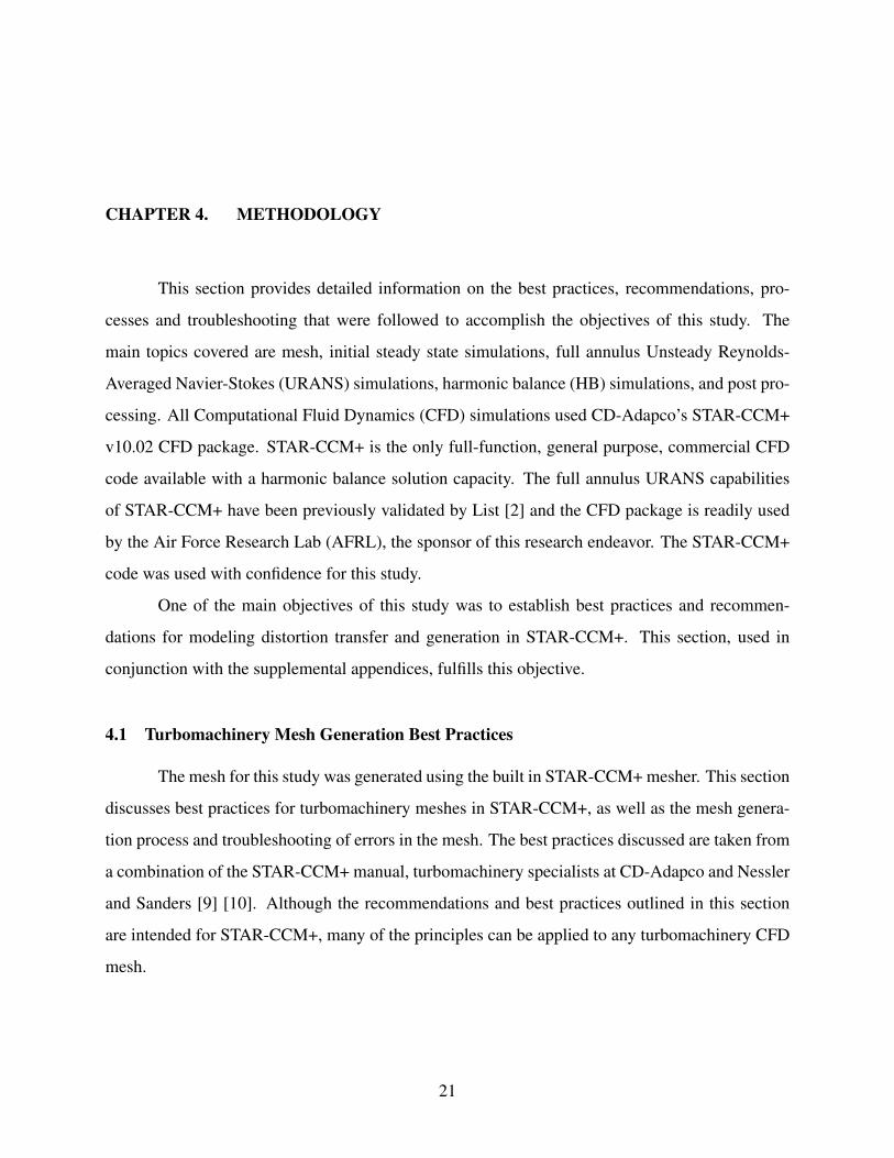
that the tip gap has sufficient resolution, it is helpful visualize the mesh. Figure 4.4 shows the tip

gap mesh of the rotor 4 mesh used in this study. This mesh was achieved by using the embedded

26

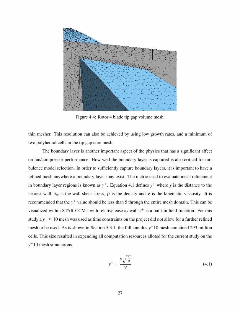
Figure 4.4: Rotor 4 blade tip gap volume mesh.

thin mesher. This resolution can also be achieved by using low growth rates, and a minimum of

two polyhedral cells in the tip gap core mesh.

The boundary layer is another important aspect of the physics that has a significant affect

on fan/compressor performance. How well the boundary layer is captured is also critical for tur-

bulence model selection. In order to sufficiently capture boundary layers, it is important to have a

refined mesh anywhere a boundary layer may exist. The metric used to evaluate mesh refinement

in boundary layer regions is known as y+. Equation 4.1 defines y+ where y is the distance to the

nearest wall, τw is the wall shear stress, ρ is the density and ν is the kinematic viscosity. It is

recommended that the y+ value should be less than 5 through the entire mesh domain. This can be

visualized within STAR-CCM+ with relative ease as wall y+ is a built-in field function. For this

study a y+ ≈ 10 mesh was used as time constraints on the project did not allow for a further refined

mesh to be used. As is shown in Section 5.3.1, the full annulus y+10 mesh contained 293 million

cells. This size resulted in expending all computation resources alloted for the current study on the

y+10 mesh simulations.

y+ =y√

τwρ

ν(4.1)

27

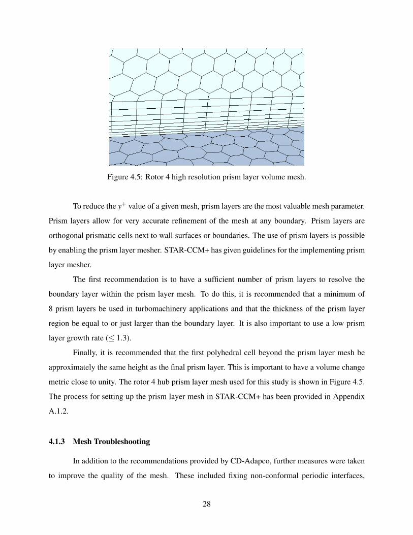
Figure 4.5: Rotor 4 high resolution prism layer volume mesh.

To reduce the y+ value of a given mesh, prism layers are the most valuable mesh parameter.

Prism layers allow for very accurate refinement of the mesh at any boundary. Prism layers are

orthogonal prismatic cells next to wall surfaces or boundaries. The use of prism layers is possible

by enabling the prism layer mesher. STAR-CCM+ has given guidelines for the implementing prism

layer mesher.

The first recommendation is to have a sufficient number of prism layers to resolve the

boundary layer within the prism layer mesh. To do this, it is recommended that a minimum of

8 prism layers be used in turbomachinery applications and that the thickness of the prism layer

region be equal to or just larger than the boundary layer. It is also important to use a low prism

layer growth rate (≤ 1.3).

Finally, it is recommended that the first polyhedral cell beyond the prism layer mesh be

approximately the same height as the final prism layer. This is important to have a volume change

metric close to unity. The rotor 4 hub prism layer mesh used for this study is shown in Figure 4.5.

The process for setting up the prism layer mesh in STAR-CCM+ has been provided in Appendix

A.1.2.

4.1.3 Mesh Troubleshooting

In addition to the recommendations provided by CD-Adapco, further measures were taken

to improve the quality of the mesh. These included fixing non-conformal periodic interfaces,

28

adjusting interface mesh density and repairing inconsistent prism layers. This section provides

recommendations to consider when troubleshooting a flawed mesh.

One issue encountered dealt with having non-conformal periodic interfaces. A conformal

match is defined at an interface and is achieved only if the vertices of the boundary mesh on one

side of the interface mate perfectly with the vertices of the boundary mesh on the other side of

the interface. For interfaces, such as the periodic interface, the failure to achieve a conformal

match can result in non-physical results and instability in the solver. The process of checking for

conformal interfaces as well as the remedy is provided in Appendix A.1.3.

The next issue encountered with the mesh dealt with the tangential resolution of the mesh

at mixing-plane interfaces. Non-reflecting boundary conditions (NRBC) are used at the simulation

outlet and the mixing plane interfaces. This feature converts the interface or boundary into annular

bins and uses a modal decomposition to extract a user specified number of modes. The zero

mode (average) is then held constant while the higher order modes are allowed to vary in order to

further resolve the physics. In order to perform the modal decomposition, a minimum tangential

resolution required to avoid aliasing exists. This resolution is calculated by means of the Nyquist

rate equation (Equation 4.2) where Nmin is the minimum number of cells in the tangential direction

and M is the number of NRBC modes set by the user.

Nmin = 2M+1 (4.2)

It was desired to solve for up to 10 NRBC modes. Therefore a minimum of 21 cells in

the tangential direction were required at all radial locations for mixing plane interfaces and at the

outlet. Initially the mesh had 18 cells tangentially at the rotor inlet near the hub. The solution to

this issue was to reduce the surface size at the rotor inlet. The spinner outlet surface size also had

to be reduced so that the surface size on both sides of the the rotor-spinner mixing-plane matched.

The process followed to adjust the surface size is provided in Appendix A.1.1.

Finally, the last mesh issue dealt with non-uniform prism layer meshes. Prism layer meshes

are designed to have very consistent thickness. If the thickness of a prism layer mesh changes

drastically, this can affect how accurately the boundary layer is captured. It was observed that the

thickness prism layers would thin out in certain areas (see Figure 4.6b) and even go to zero near

29

(a) Rotor exit mixing-plane (green), hub (gray). (b) Rotor periodic interface.

Figure 4.6: Non-uniform prism layer observed in preliminary mesh.

certain boundaries (see Figure 4.6a). This was fixed by increasing the boundary layer march angle

to the upper limit and decreasing the prism layer thickness (reducing the prism layer can only be

done if by doing so the thickness does not drop below the physical boundary layer thickness). The

processes for reducing prism layer thickness and adjusting the boundary march angle are provided

in Appendices A.1.2 and A.1.4 respectively.

4.2 Initial Steady State Solution

Prior to converging either the full annulus URANS or the HB simulations, a single passage

steady state mixing-plane simulation was converged. This simulation was then used as an initial

solution for the URANS and HB simulations. This process is recommended as it expedites the

convergence process for both of these simulation types and the computational cost of achieving

a converged steady state mixing-plane solution is relatively cheap when compared to the HB and

URANS simulations. This section outlines the process followed to achieve a converged steady

state mixing-plane simulation.

The computational domain for the steady state mixing-plane simulations varied. Converged

simulations which included regions for the full annulus spinner, single passage rotor and single

passage stator were used as initial solutions for the full annulus URANS simulations (see Figure

4.7a). The HB simulations did not require the full annulus inlet, so this was excluded in the initial

steady state solution (see Figure 4.7b). The reasoning behind this will be discussed in great detail

in Section 4.4.

30

(a) Right to left: spinner, rotor, stator. (b) Right to left: rotor, stator.

Figure 4.7: Single passage computational domains (a) with spinner region and (b) without.

Table 4.2: Mixing-plane meshcell count (single rotor

and single statorpassage).

Region Cell Count

Spinner 14.9 MRotor 4.6 MSpinner 6.0 M

Total 25.5 M

The mesh used for all steady state mixing-plane simulations was an unstructured mesh

generated in STAR-CCM+ using all of the recommendations outlined in Section 4.1. The mesh

statistics are listed in Table 4.2. As mentioned before, full annulus simulations included the spinner

region and the HB simulations did not.

Once the mesh had been generated and the periodic interfaces were verified as conformal

(see Section 4.1.3), the appropriate physics models were selected, boundary conditions set, solver

parameters adjusted and the simulation was converged. The process used to achieve this is found

in A.2

31

Table 4.3: Full annulus meshcell counts (1 spinner,

20 rotor and31 stators).

Region Cell Count

Spinner 14.9 MRotor 92.3 MStator 185.9 M

Total 293.1 M

4.3 Full Annulus URANS

Two full annulus URANS simulations were converged for this study.The first simulation

used the 7.5% distortion profile (Figure 3.2a) and was used as a baseline to compare the HB

simulations against. A simulation using the 15% distortion profile (Figure 3.2b) was also run to

evaluate the effects of increasing distortion intensity on distortion transfer and generation. The

computational domain of the full annulus simulations include 3 regions: the spinner, rotor and

stator (see Fig. 3.1). The unstructured full annulus mesh for both simulations was generated from

the steady state mixing-plane mesh. The mesh statistics are given in Table 4.3.

4.3.1 Full Annulus Process

This section gives the general process for setting up, running and converging a full annulus

URANS simulation with a total pressure inlet distortion profile. The detailed step-by-step process

has been provided in Appendix A.3.

First, the full annulus mesh is generated. This starts with the initial steady state solution

described in Section 4.2. The rotor and stator regions are replicated and translated to produce

the full annulus domain. Next the appropriate interfaces are generated, mesh set to rotating, time-

accurate unsteady solver connected and the inlet distortion profile is applied. Finally, solver criteria

are set and the solver converged.

32

4.4 Harmonic Balance

Multiple HB simulations were converged using the 7.5% distortion profile (Figure 3.2a) and

various mode combinations. The combinations used and the significance of the mode combinations

are described in this section. The computational domain for the HB simulations are identical

to the steady state mixing-plane simulations described in Section 4.2 and shown in Figure 4.7b.

This section provides more in-depth information about the nomenclature, reasoning behind the

simulations run, as well as the processes for set up and convergence of HB simulations.

4.4.1 Blade Rows

Blade rows are used by the HB solver to specify the rotation rate and number of blades of

each region. The number of blades in a blade row does not represent the actual physical number

of blades, but the fraction of the circumferential domain that has been modeled. For example, the

rotor region represents 1/20th of the circumferential domain. Therefore the blade row connected

to the rotor region has 20 blade rows. For the full annulus inlet, the entire circumferential domain

has been modeled so the number of blades in the blade row is one.

Blade rows are different from regions because multiple regions can share the same blade

row given they have the same number of blades and the same rotation rate. For example, if the

computational domain included a full annulus spinner region and a full annulus exit region, both

of these regions would have a rotation rate of zero rpm and one blade. Therefore, both of these

regions should be assigned to the same blade row even though they are separate regions.

4.4.2 Modes

Prior to passing flow field information across interfaces, the HB solver expands the infor-

mation in the form of Fourier series. The number of modes in a blade row specifies the number

of terms that will be used in the Fourier series representation of the data. If 2 modes are specified

for a blade row, then the Fourier series representation of that blade row would use the +2, +1, 0,

-1 and -2 terms (positive referring to the real values in the exponential Fourier series and negative

referring to the imaginary values in the exponential Fourier series). The more modes, the higher

the resolution of the information being passed across the interfaces.

33

In this thesis, mode combinations used for a given simulation are referenced for the inlet

boundary condition and each blade row in the stream wise direction. For example, an HB simula-

tion with 3 modes for the inlet boundary condition, 2 modes for the rotor blade row and 1 mode

for the stator blade row would be referred to as a 3-2-1 simulation. This notation is useful when

describing HB best practices.

An important clarification to be made is that using more modes in a blade row region does

not affect the resolution of that blade row. This is because the modes only specify how the flow

field information of that particular blade row is passed to the other blade rows, not the resolution

of the solution within that region. For example consider two simulations, one with 0 modes in the

rotor blade row and 0 modes in the stator blade row (0-0), and another simulation with 5 modes

specified in the rotor blade row and 0 in the stator blade row (5-0). The flow field in the rotor region

would look exactly the same for both simulations because the number of modes in the rotor does

not affect the rotor solution. Also, the number of modes in the stator region did not change, so the

information passed from the stator to the rotor is identical in both cases. On the other hand, the

flow field in the stator region would look drastically different between the two simulations because

the resolution of the rotor information passed to the stator is drastically different. In the (0-0)

simulation, no blade row effects from the rotor would be visible in the stator region. However,

with the (5-0) simulation, the blade row effect would be very apparent in the stator region. This

effect is illustrated in 4.8. To expand on this example, a (0-0) simulation would have the same

answer as a mixing-plane simulation since the zero mode is the average of the flow. This is the

same way that the mixing-plane interface passes information.

Recommendations for selecting the mode combination for a given simulation depending

on what is desired to be captured are given in section 5.3.

4.4.3 Wake Specification

The wake specification is a boundary condition unique to the HB solver. A wake specifica-

tion allows the user to specify an inlet or outlet condition with a prescribed distortion and rotation

rate. This boundary condition does not require a full annulus region to set a full annulus distortion

profile. Since all HB simulations run used the wake specification method to set the inlet distortion

profile, the full annulus spinner region was not included in the computational domain.

34

(a) Without rotor modes (0-0).

(b) With rotor modes (5-0).

Figure 4.8: Example of the effect of modes in the rotor blade row on the solution.

The wake specification is set different than traditional inlet boundary conditions. Gauge

total pressure and absolute total temperature are set as the circumferential average values only

(also known as the zero mode). The circumferential averages of total pressure and total temper-

ature generated for the HB simulation wake specifications are shown in Figure 4.9. Distortion is

set in terms of circumferential variations in static pressure, static temperature and velocity. The

circumferentially varying parameters used to set the wake specification are shown in Figure 4.10.

The circumferential averages of static pressure, static temperature and velocity are allowed to vary

to resolve the flow field. The number of modes used to represent the wake specification boundary

condition can be set, allowing for the resolution of the the distortion profile to be adjusted.

When setting up the wake specification, it was assumed that static pressure would be con-

stant in the circumferential direction (see Figure 4.10a). Using this assumption, it is possible to

generate the static pressure, static temperature and axial velocity profiles that correlate with the

35

(a) (b)

Figure 4.9: Circumferential average of a) gauge total pressure and b) absolute total temperatureused for the wake specification for all HB simulations.

(a) (b) (c)

Figure 4.10: Circumferential variation in a) static pressure, b) static temperature and c) axialvelocity used for the wake specification for all HB simulations.

chosen total pressure distortion profile by solving Equations 4.3, 4.4 and 4.5. In these equations,

Pt represents total pressure, P represents static pressure, γ represents the isentropic expansion fac-

tor, M represents Mach number, Tt represents total temperature, T represents static temperature, V

represents velocity and R represents the ideal gas constant.

Pt = P

(1+

γ−12

M2

) γ

γ−1

(4.3)

36

Table 4.4: Time levels for a (2-0) simulation.

Time Level Rotor Modes Stator Modes

1 -2 02 -1 03 0 04 1 05 2 0

Tt = T

(1+

γ−12

M2

)(4.4)

M =V√γRT

(4.5)

As will be shown in Section 5.3, assuming constant circumferential static pressure was

sufficient for modeling the inlet distortion profile for the HB simulations. Another method inves-

tigated but not implemented for generating the wake specification profile is to run a full annulus

URANS simulation first. From this simulation, total pressure, total temperature, static pressure,

static temperature and axial velocity at the inlet to the rotor can all be extracted. The circumferen-

tial average of total pressure and total temperature are then taken at radial bins and saved as a .csv

file containing the average values and the radial locations. The circumferential variations in static

pressure, static temperature and axial velocity were then saved as a separate .csv file.

4.4.4 Time Levels

Time levels are another parameter unique to the HB solver. Time levels represent the

number of discrete steady state solutions that must be solved for the HB solver to conduct a Fourier

transform on the unsteady behavior. The more modes that are specified in a given region, the more

time levels that have to be solved for with each iteration in order to calculate the higher fidelity

Fourier transform. This effect is illustrated in Tables 4.4 and 4.5 where the number of time levels

are shown for a (2-0) simulation and a (2-1) simulation. Notice that by increasing the number of

modes in a single region, the number of time levels triples.

37

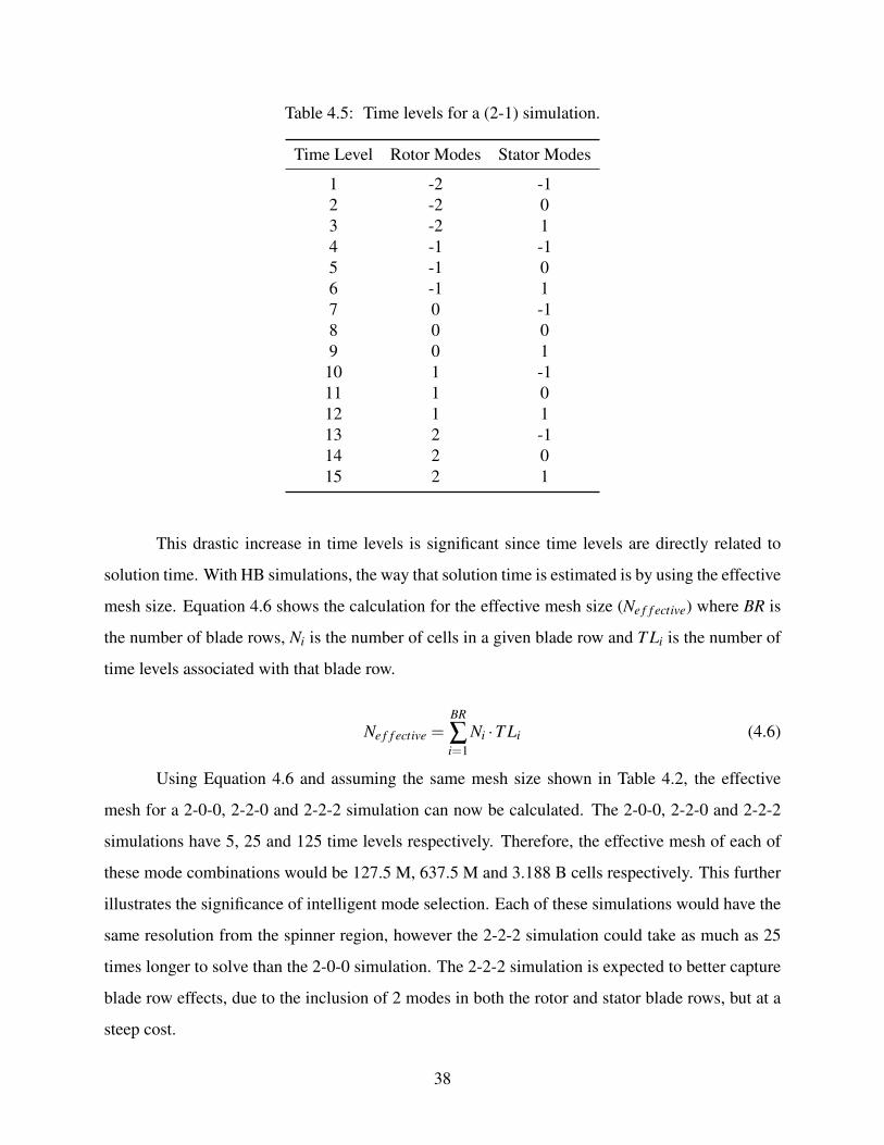
Table 4.5: Time levels for a (2-1) simulation.

Time Level Rotor Modes Stator Modes

1 -2 -12 -2 03 -2 14 -1 -15 -1 06 -1 17 0 -18 0 09 0 1

10 1 -111 1 012 1 113 2 -114 2 015 2 1

This drastic increase in time levels is significant since time levels are directly related to

solution time. With HB simulations, the way that solution time is estimated is by using the effective

mesh size. Equation 4.6 shows the calculation for the effective mesh size (Ne f f ective) where BR is

the number of blade rows, Ni is the number of cells in a given blade row and T Li is the number of

time levels associated with that blade row.

Ne f f ective =BR

∑i=1

Ni ·T Li (4.6)

Using Equation 4.6 and assuming the same mesh size shown in Table 4.2, the effective

mesh for a 2-0-0, 2-2-0 and 2-2-2 simulation can now be calculated. The 2-0-0, 2-2-0 and 2-2-2

simulations have 5, 25 and 125 time levels respectively. Therefore, the effective mesh of each of

these mode combinations would be 127.5 M, 637.5 M and 3.188 B cells respectively. This further

illustrates the significance of intelligent mode selection. Each of these simulations would have the

same resolution from the spinner region, however the 2-2-2 simulation could take as much as 25

times longer to solve than the 2-0-0 simulation. The 2-2-2 simulation is expected to better capture

blade row effects, due to the inclusion of 2 modes in both the rotor and stator blade rows, but at a

steep cost.

38

4.4.5 Harmonic Balance Simulations

For this study multiple mode combinations were run to evaluate the capabilities and cost of

the HB solver. A 5-0-0 simulation was chosen first because it only passes the the distortion from

the inlet boundary condition between regions. Blade row interactions are averaged out, therefore,

the inlet distortion profile is prioritized over blade row interactions. Next, the 2-2-2 simulation was

chosen because it puts more priority on blade row interactions than the 5-0-0 simulation. Finally,

the 3-1-1 simulation was chosen as a balance between the 5-0-0 and 2-2-2 simulations. With 3

modes for the inlet boundary condition, the 3-1-1 simulation uses a resolution in-between the 5-

0-0 and 2-2-2 simulations to model and pass inlet distortion effects through the blade rows. The

resolution of blade row effects captured in the 3-1-1 simulation is also between the 5-0-0 and 2-2-2

simulations with 1 mode in each blade row.

4.4.6 Harmonic Balance Process

This section gives the general process for setting up, running and converging an HB sim-

ulation with a total pressure inlet distortion profile. The detailed step-by-step process has been

provided in Appendix A.4.

The process begins with the initial steady state solution described in Section 4.2. The HB

physics model is then set up and connected. Next, the wake specification boundary condition is

set and steps are taken to prepare for post processing. Finally the solver parameters are set and the

simulation is converged.

4.5 Post Processing

Post processing was required on all simulations to qualitatively and quantitatively represent

the CFD data. This section outlines the methods used for time averaging, mass flow time averaging,

extracting tradition distortion descriptors and conducting Fourier analysis.

39

4.5.1 Time Averaging

Much of the data from both the full annulus and HB simulations needed to be time aver-

aged. The time averaged values were used for distortion transfer and generation analysis. There

are a couple of ways to time average data from a time-accurate simulation. This section gives

the general process implemented to achieve time averaged results. For the detailed step-by-step

process see Appendix A.6.

For the full annulus simulations, time-accurate data must first be extracted. For the full

annulus simulation this is done by creating internal tables with an update frequency that will save

desired scalar values at specified intervals. For this project static pressure, static temperature , total

pressure, total temperature and axial velocity were exported every 1 degree of rotation of the rotor

for a full wheel at the rotor inlet, stator inlet and stator outlet.

Once the time-accurate data had been exported, each of the data files are then structured

and averaged temporally.

The data from the HB simulations also needed to be time averaged to compare against the

full annulus data. To do this it was necessary to extract full annulus time-accurate information, as

was done for the full annulus simulations. This was done using the HB solution views. HB solution

views allow the user to visualize a full annulus time-accurate representation of the HB solution.

No physical time marching is required. Figure 4.11 shows a visualization of an HB solution view

for a 5-0-0 simulation.

The same tables used for the full annulus time averaging were produced for each of the HB

simulations. A java script was generated to change the physical time of the HB solution view so

that the rotor would rotate 1 degree and then export the table. The same time averaging MATLAB

script used for the full annulus simulation was then used for the HB simulations.

4.5.2 Mass Flow Time Averaging

For certain performance parameters, it was necessary to not only time average the data, but

also to mass flow time average the data. This is also know as mass-averaging. The equation for

the mass flow average of a given parameter φ is shown in Equation 4.7, where φ f is the face value

40

Figure 4.11: HB Solution view representation of HB 5-0-0 at a constant radius of 0.175m (75%span of the rotor leading edge).

of the selected scalar, ρr is the face density, v f is the face velocity vector and a f is the face area

vector.

MassFlowAverage =∑ f ρ f φ f |v f ·a f |∑ f ρ f |v f ·a f |

(4.7)

A mass flow time average represents both the spatial and temporal average of a given pa-

rameter for a specified time window and area. The mass flow time averages for this study were

averaged over one rotor revolution (2.97 ms) and at three locations (rotor inlet, stator inlet and sta-

tor outlet). The mass flow time averaged values are useful for calculating performance parameters

such as fan pressure ratio and efficiency.

The method used for mass flow time averaging the data for the full annulus simulations

involved generating mass flow average monitors for total pressure and total temperature at the rotor

inlet, stator inlet and stator outlet prior to exporting time-accurate information. These monitors

were set to write to the output file. The simulation was then allowed to run for a full wheel. Upon

41

Figure 4.12: 15% total pressure distortion at 50% span with SAE-ARP 1420-b values reported.

completion of the wheel, the values written to the output file at each time step were averaged to

attain the mass flow time averaged values.

The method used for mass flow time averaging the HB simulations is the same as the full

annulus simulation with the exception of using the HB solution view to construct the full annulus

representation.

4.5.3 Tradition Distortion Descriptors

The traditional SAE-ARP 1420-b [8] distortion descriptors discussed in Section 2.2.1 were

used initially to quantify distortion transfer and generation. The numerical values were calculated

using radial bins from the time averaged CFD data using Equations 2.1 and 2.2. The percent span

time averaged data was then plotted along with PAV and PAV LOW . Intensity, extent and peak-to-

peak amplitude were also reported on the plot. An example of one of these plots is shown in Figure

4.12.

42

4.5.4 Fourier Analysis

Fourier analysis was used to analyze distortion transfer and generation for all full annulus

and HB simulations. The specific Fourier quantities evaluated in this study are the modal am-

plitude, total amplitude and phase shift. Each of these quantities were calculated from the time

averaged data by extracting from the Fourier series representation of the profile. The Fourier series

was extracted using a discrete Fourier transform, which was conducted in MATLAB. The Fourier

series equation used is shown in Equation 3.3, where An represents the modal amplitude of mode

n, φn the modal phase of mode n.

sN(x) =A0

2+

N

∑n=1

An · sin(2πnx

P+φn

)(3.3)

An inherent characteristic of the Fourier series is that each mode is statistically independent

of all other modes [7]. This means that the magniude and phase of any mode in the Fourier series

is not dependent on the magnitude and phase of any other modes. The value of this is that it

allows the Fourier components to be evaluated on a mode-to-mode basis (also known as a modal

analysis). This is a powerful aspect of Fourier analysis. The modal analysis was conducted using

the modal amplitude and phase. Each of these components gives detailed information about the

magnitude and phase of a given mode. To better understand this physical interpretation, the inlet

total pressure profile shown in Figure 3.2b has been plotted along with the Fourier modes in Figure

4.13. The amplitude and phase of each component has also been tabulated in Table 4.6. By viewing

the figure and table, it is observed that mode 1 is the dominant mode and that modes 4 and 8 are

almost negligible. This is a characteristic of a quarter square wave, which the 90◦ sector closely

resembles.

The modal amplitudes listed in Table 4.6 can also be plotted as a bar plot with the modal

amplitudes at downstream locations. Figure 4.14 show this and is a valuable tool for comparison

of modal values.

The sum of all modes in the Fourier series produces the reconstructed representation of

the periodic profile. This is illustrated in Figure 4.13. Here, 8 modes are used to reconstruct the

time averaged profile. If infinite modes are used in the reconstruction, the reconstructed profile

would perfectly match. This characteristic of the Fourier series along with the fact that each mode

43

(a) Modes 1-4

(b) Modes 5-8

Figure 4.13: Fourier modes of the 15% total pressure distortion profile at 50% span.

44

Table 4.6: Fourier modal descriptors forthe 15% total pressure distortion

profile at 50% span.

Mode Amplitude (kPa) Phase (degrees)

0 69.0 N/A1 4.67 1802 3.32 1803 1.63 1804 0.16 1805 0.69 2166 0.87 2107 0.56 2058 0.11 202

Figure 4.14: Fourier modal amplitude for the 15% total pressure distortion profile at 50% span forthe rotor inlet, stator inlet and stator outlet.

is statistically independent illustrates that every mode effects the distortion. Also the sum of all

modes represents the true profile. Therefore, by summing all modal amplitudes, a single value can

be obtained to describe the total amount of distortion present in a given profile. This value is called

the total amplitude and it is a measure of both the magnitude and severity of a distortion profile.

45

The equation for total amplitude is shown in Equation 4.8, where ΣA is the total amplitude, N is

the number of Fourier modes present and An is the modal amplitude of mode n.

ΣA =N

∑n=1

An (4.8)

46

CHAPTER 5. RESULTS

This section details the results and analysis of this study. This section is divided into three

main results discussions. The first is the evaluation of distortion descriptors, followed by the

comparison of the 7.5% and 15% full annulus URANS simulation and finally the comparison and

evaluation of the HB simulations versus the 7.5% full annulus URANS simulation.

5.1 Evaluation of Distortion Descriptors

The purpose of distortion descriptors are to quantitatively describe the distortion physics.

The value of a quantitative description of the distortion physics is it allows for an unbiased assess-

ment of the physics. This assessment increases understanding of the underlying physics and allows

for predictive numerical and analytical models to be developed based on this better understanding.

In many previous research studies [4] [5] [6], much of the distortion analysis has been conducted

from a qualitative standpoint (ex. contour plots of flow features, description of distortion shape).

This is due to a lack of robust descriptors that accurately describe distortion physics. Qualitative

analysis is valuable and is regularly performed in the current study. However, it does not lend

itself to analytical and numerical methods such as predictive models. This, in conjunction with the

fact that qualitative analysis must be conducted on a case by case basis, makes process automation

impossible. Qualitative analysis is also prone to bias, reducing it’s reliability. In order to cre-

ate robust predictive models for distortion transfer (total pressure), generation (total temperature)

and the effects of distortion on performance parameters, accurate, versatile, quantitative distortion

descriptors must be identified.

Four key parameters have been identified in this study as desirable to quantitatively capture

distortion transfer, generation and effects on performance. These four parameters are distortion

magnitude, shape, severity and phase. The definition of each of these parameters as well as their

significance is as follows:

47

1. Magnitude is a measure of the amplitude of a given distortion profile. A qualitative example

of distortion magnitude would be the peak-to-peak amplitude of a sinusoidal pattern. This

parameter is crucial to understanding how a distortion profile is generated and dissipated as

it is transferred through the fan/compressor. It is also a valuable parameter required to un-

derstand how the magnitude of a profile affects fan/compressor performance parameters. For

the distortion magnitude parameter to be used in these capacities it must be robust enough to

describe any type of distortion profile with accuracy.

2. Shape is a quantitative description of the shape of a given distortion profile. Some qualitative

examples of circumferential distortion shape are sinusoidal, 1 per-rev and 90◦ sector. This

parameter is crucial to understanding how the shape of the distortion profile is altered as it

passes though a rotor or stator region. The shape of a profile also has a direct effect on the

performance of the downstream fan/compressor. This metric must be able to describe any

given profile shape to be viable.

3. Severity is a measure of how much distortion is present. Severity is a function of both

magnitude and shape. An example of this is a sinusoidal, 1 per-rev profile with the same

peak-to-peak amplitude as a 1 per-rev square wave. Each of these profiles may have the

same magnitude, however, the more severe gradients in the square wave will likely have

more of an adverse affect on the downstream fan/compressor than the sinusoidal profile.

This parameter is critical for creating robust models for predicting the effects of distortion

profiles on engine performance. This metric would also aid in better understanding distortion

transfer and generation physics. For this parameter to be viable, it needs to be robust enough

to capture the severity of any given profile magnitude or shape with accuracy.

4. Phase shift is a measure of the rotational translation of a given distortion profile. This pa-

rameter is valuable for understanding the translational motion of the distortion profile as it

passes through the fan/compressor. This is important to be able to quantify since often there

is a phase lag between the total pressure and total temperature distortion. It is also necessary

to be able to predict rotational motion of distortion profiles.

When used in conjunction, these four parameters would be valuable assets for better un-

derstanding distortion transfer, generation and for creating analytical and numerical models for

48

predicting effects on fan/compressor performance. This section discusses the ability of the SAE-

ARP distortion descriptors and the derived Fourier descriptors to quantify these metrics. This

section focuses on analyzing the SAE-ARP distortion descriptors and the derived Fourier descrip-

tors’ ability to capture distortion magnitude, shape, severity and phase. The physical significance

and interpretation of the results will be discussed in Sections 5.2 and 5.3

5.1.1 SAE-ARP 1420-b Descriptors

The current standard in industry for describing distortion is the SAE-ARP 1420-b distortion

descriptors [8]. The two metrics are intensity and extent. The development of these metrics along

with their designed use and the equations used to calculate them are described in depth in Section

2.2.1. These metrics were used in preliminary post-processing to evaluate their ability to capture

magnitude, shape, severity and phase of the CFD distortion data.

The first data set analyzed was the time averaged 15% full annulus URANS data for total

pressure and total temperature. The distortion descriptors were calculated at 50% span at the

rotor inlet, stator inlet and stator outlet for total pressure and total temperature. Each of these are

plotted in Figures 5.1 and 5.2. The x-axis of both sub-figures corresponds to the circumferential

location around the engine annulus with 180◦ being top dead center (TDC). Solid lines represent

the time averaged data. Dashed lines represent the circumferential average pressure (PAV ) in Figure

5.1 and the circumferential average temperature (TAV ) in Figure 5.2. Dotted lines represent the

circumferential average of all values below the average for pressure (PAV LOW ) in Figure 5.1 and

for temperature (TAV LOW ) in Figure 5.2. Line color corresponds to the data set the line represents;

red, blue and green corresponding to the rotor inlet, stator inlet and stator outlet respectively.

The SAE-ARP metrics, intensity (I) and extent (Θ), along with the peak-to-peak (Pk−Pk)

magnitude of the profile are reported on each figure. The subscript notation for each of these

metrics represents the axial location that the metric corresponds to; 1, 2 and 3 corresponding to the

rotor inlet, stator inlet and stator outlet respectively.

49

Figure 5.1: SAE-ARP descriptors applied to distortion transfer for the time averaged 15% fullannulus URANS data at 50% span for the rotor inlet, stator inlet and stator outlet profiles.

Intensity

The first descriptor evaluated was intensity. As can be seen in Figure 5.1, the total pressure

intensity at the rotor inlet is 9.8%. This is a reasonable description of the inlet amplitude as the

total pressure peak-to-peak at this location is 10.8 kPa which is 15% of the maximum total pressure.

Since the intensity only describes low distortion, an intensity of 9.8% is a reasonable quantification

of the magnitude.

The same trend is observed for total temperature at the rotor inlet. From a qualitative

assessment of the total temperature profile at the rotor inlet shown in Figure 5.2, the magnitude

of this distortion profile is observed to be 0. This agrees with the intensity calculation of 0%

50

Figure 5.2: SAE-ARP descriptors applied to distortion generation for the time averaged 15% fullannulus URANS data at 50% span for the rotor inlet, stator inlet and stator outlet profiles.

also shown in this figure. Therefore, magnitude is reasonably described by intensity for both total

pressure and total temperature at the rotor inlet. This is due to the fact that both of these profiles

have either a clearly defined low distortion region, or no distortion. However, when applied to

distortion profiles without clearly defined low distortion regions, the intensity descriptor becomes

less accurate at describing profile magnitude.

A qualitative assessment of the stator inlet total pressure distortion profile shown in Figure

5.1, gives the impression that the magnitude of the distortion is approximately greater than or

equal to the magnitude of the rotor inlet. The intensity does not capture this behavior. The total

pressure intensity at the stator inlet location is 4.66%. This is a factor of 2 lower than the intensity

at the inlet and does not agree with the qualitative assessment of the profile. The cause of this

51

disconnect is related to how intensity is calculated (see Equation 2.1). Since intensity is a measure

of low distortion only, as the profile reshapes to include both low and high pressure distortion, the

intensity metric only captures the low pressure distortion. This was not an issue at the rotor inlet

as distortion of this profile is dominantly low pressure distortion.

Another cause of this inaccuracy is due to the pressure rise. Intensity is calculated as a

fraction of the circumferential average. This means that even if the shape and magnitude of a

distortion profile are held constant, but the circumferential average is increased by a factor of two,

the intensity of that profile will be half its original value.

The issues seen with the intensity descriptor are further exacerbated at the stator exit, as

can be seen in Figure 5.1. The total pressure intensity at the stator exit location is 4.93%. This is

slightly increased from the stator inlet intensity of 4.66%. A visual inspection of the stator exit total

pressure profile shows that there are blade row effects present. This is due to the fact that the stator

blades are stationary in the computational domain. Therefore, the wake effects from the stator

blades are still present in the distortion profile, even after time-averaging. These perturbations act

as a 31 per-rev distortion profile. While blade row effects are a form of distortion, when analyzing

distortion transfer and generation, what is of the most interest is how the inlet distortion profiles

change through the fan/compressor. Since the intensity calculation has no method for filtering, it

is difficult to determine whether the increase in intensity observed is physical or a false increase

caused by the blade row effects. The uncertainty in the intensity illustrates that the descriptor

is not robust enough to reliably capture the magnitude of the distortion profile when blade row

perturbations are present in the time-averaged profile.

The intensity of the total temperature distortion at the stator inlet and the stator outlet also

does not accurately represent the magnitude of the distortion. As can be seen in Figure 5.2, the

intensity at the stator inlet and stator outlet is 0.67%. However, the peak-to-peak amplitude is

22.0 K and 21.6 K respectively. These peak-to-peak values are more than 6% of the average total

temperature at the stator inlet and stator outlet. Therefore, the intensity values are an order of

magnitude less than the percent amplitude of the peak-to-peak values. This inaccuracy in describ-

ing the magnitude of the distortion is caused by majority of the total temperature distortion being

greater than the undistorted range (90◦ to 270◦). Since intensity only captures low distortion, the

high distortion range is not captured. This further illustrates that the intensity descriptor is not

52

robust enough to capture the magnitude of all profile types. profiles with high distortion and blade

row effects are not well described by the intensity descriptor.

Extent

The next descriptor evaluated was extent. As can be seen in Figure 5.1, the total pressure

extent at the inlet to the rotor region is 96◦. A qualitative analysis of the rotor inlet total pressure

distortion profile agrees with this value. It is know that the inlet distortion profile used for this

study is a total pressure 90◦ sector (see Figure 3.2b). Therefore, it is expected that the total pressure

extent at the inlet should be close to 90◦. However, the same agreement is not observed for total

temperature.

As can be seen in Figure 5.2, the total temperature extent at the rotor inlet is 189◦. However,

a qualitative assessment of the profile shows that there is no distortion present and therefore, the

extent should not be defined. This brings to light an issue with extent. The extent metric only has

a physical meaning as long as the intensity is non-zero.

Additional shortcomings of the extent metric are discovered as the stator inlet and stator

outlet profiles are evaluated. As can be seen in Figure 5.2, the total temperature extent is 252◦

at the stator inlet and 253◦ at the stator outlet. From qualitatively analyzing the stator inlet and

outlet profiles, it can be observed that the profile shapes and magnitudes are approximately equal

to each other. Therefore, a minimal change in extent between the stator inlet and exit is expected.

However, it can also be seen by viewing the profiles that the range of the distorted region for both

profiles is approximately half of the circumferential domain (or 180◦). Therefore, extent values

of 252◦ and 253◦ do not accurately represent the distorted range of the profiles. The cause of this

disconnect is related to the reshaping of the distortion profiles. At the stator inlet and stator outlet,

high and low distortion have become prominent in both total pressure and total temperature. This

shifts the average above the non-distorted portions of these profiles (from 0-90◦ and 300-360◦).

Therefore this non-distorted region is included in the extent calculation.

Another issue with the extent metric is that, like intensity, extent has no filtering methods.

This issue can be seen in Figure 5.1. The extent values of 111◦ and 137◦ for the stator inlet

and stator outlet respectively, are in a reasonable range given the extent of the rotor inlet is 96◦.

However, like was observed in the total temperature profiles, a qualitative analysis of the total

53

pressure profiles indicates that the extent at the stator inlet should be approximately equal to the

extent at the stator exit. This is not the case and the cause is due to the 31 per-rev perturbations

present in the stator exit profile. The extent calculation includes all circumferential ranges where

the time accurate data is below the mean. This causes the extent metric to overshoot the actual

value when the 31 per-rev perturbations are present.

The evaluation of the SAE-ARP distortion descriptor’s ability to capture magnitude, shape,

severity and phase is considered poor. The intensity and extent descriptors are not robust. Both

struggle to perform when the profile shape is not a clearly defined low distortion region. These

descriptors also have no means of filtering out blade row effects, resulting in unreliable or biased

values when such effects are present. These descriptors also have no means of capturing or de-

scribing shape or phase. These descriptors are not recommended for broad implementation of a

multistage analysis of distortion transfer and generation.

5.1.2 Fourier Analysis for Describing Distortion

Upon researching alternative quantification techniques, Fourier analysis was investigated.

Fourier analysis was a natural choice since fans and compressors are inherently periodic both

spatially and temporally. This is due to the fact that these are rotating systems. Fourier analysis

excels at quantifying periodic behavior and has therefore been implemented into many scientific

fields including signal processing, imaging, statistics, cryptography and heat transfer.

Through the investigation of Fourier analysis, this method was identified as superior for

quantifying distortion transfer, and generation than the SAE-ARP 1420b descriptors. Three spe-

cific Fourier quantities were identified as showing promise; namely modal amplitude (Ai), total

amplitude (ΣAi) and phase shift (∆φi). The calculation of these quantities is described in detail in

Section 4.5.4.

Each of these Fourier descriptors have been plotted in Figure 5.3 and 5.4. The same data set

as was plotted in Figures 5.1 and 5.2 has been used for this analysis for the purposes of comparison.

The same axis and coloring format has been used. However, dotted lines now represent the 12

mode Fourier series representation (reconstruction) of the distortion profile. 12 Fourier modes

were chosen to illustrate the Fourier series ability to match the distortion profile and also filter

out blade row perturbations. Since there are 20 rotor blades and 31 stator blades in the rotor 4

54

Figure 5.3: Fourier descriptors applied to distortion transfer for the time averaged 15% fullannulus URANS data at 50% span for the rotor inlet, stator inlet and stator outlet profiles.

geometry, if 20 modes are used, rotor perturbations will be captured by the Fourier series and if 31

modes are used, stator perturbations will be captured by the Fourier series. It was desired to model

how the inlet distortion profiles change through the fan and not to capture blade row perturbations,

so 12 modes were found to be sufficient through visual inspection of the profile.

The notation for the modal amplitude values consist of two subscripts. The first subscript

represents the axial location; rotor inlet, stator inlet and stator outlet being 1, 2 and 3 respectively.

The second subscript refers to the harmonic mode. Modes 1, 2 and 3 are reported in this figure as

these are the dominant (highest amplitude) modes. The significance of the dominant modes will

bee discussed later in this section. By this notation, A3,2 represents the amplitude of mode 2 at the

55

Figure 5.4: Fourier descriptors applied to distortion generation for the time averaged 15% fullannulus URANS data at 50% span for the rotor inlet, stator inlet and stator outlet profiles.

stator outlet (location 3). The subscript notation for total amplitude only indicates axial location as

this parameter is not mode dependent.

The subscript notation for the phase shift is similar to the subscript notation for the modal

amplitudes. The first subscript represents the two locations that the change in phase is being

reported for. The second subscript is the harmonic mode. By this notation ∆φ1−2,3 would be the

phase shift from the rotor inlet to the stator outlet for mode 3. The phase shift at the rotor inlet is

not reported since phase shift is relative to the previous axial location and the rotor inlet is the first

axial location reported.

The modal amplitudes for total pressure and total temperature have also been plotted in

Figure 5.5. Rotor inlet, stator inlet and stator outlet are represented by red, blue and green re-

56

(a) Total pressure.

(b) Total temperature.

Figure 5.5: Fourier modal amplitudes applied to distortion transfer and generation for the timeaveraged 15% full annulus URANS data at 50% span for the rotor inlet, stator inlet and statoroutlet profiles.

57

spectively. 8 modes have been plotted in this figure as these are sufficient for the modal analysis

conducted. All modes greater than 8, with the exception of modes 20 and 31 (the fundamental

frequencies of the rotor and stator respectively), have an amplitude less than 0.25 kPa and 0.25 K

for total pressure and total temperature respectively. This amplitude is minimal compared to the

maximum mode 1 amplitudes of 6.15 kPa and 4.1 K.

Modal Analysis

The first analysis conducted is a modal analysis of the modal amplitude and phase. As

can be seen in Figure 5.3, the total pressure modal amplitudes at the rotor inlet are 4.67 kPa, 3.32

kPa and 1.63 kPa for modes 1, 2 and 3 respectively. The amplitudes of each mode represents the

effective amplitude of that per-rev component. By this analysis, the rotor inlet has an effective 1

per rev amplitude of 4.67 kPa, 2 per-rev amplitude of 3.32 kPa and an effective 3 per-rev amplitude

of 1.63 kPa. This quantifies the magnitude of the distortion profile on a mode to mode basis.

The relative amplitudes also gives information about the shape of the profile as each mode

has a specific shape it coincides with. Therefore by identifying the dominant (highest amplitude)

mode, the general shape of the profile can be identified. By this analysis, the mode one amplitude

is the greatest at the rotor inlet, inferring that the shape of the profile is dominantly a 1 per-rev

profile. A visual inspection of the profile confirms this observation.

The modal amplitudes change through the rotor to 5.15 kPa, 3.82 kPa and 1.18 kPa at the

stator inlet for modes 1, 2 and 3 respectively. The modal amplitude of mode 1 increases by 480

Pa (10.3%) and mode 2 by 500 Pa (15%). Meanwhile, the modal amplitude for mode 3 decreased

by 450 Pa (27.6%). This inconsistent change in modal amplitude across the modes signifies a

significant change in the profile shape, which is confirmed upon viewing the time averaged profile

at the stator inlet. This change in amplitude can also be visualized in Figure 5.5a. This figure

shows that modes 1, 2, 4, 5 and 8 increase in amplitude while modes 3,6 and 7 decrease inferring

a shape change.

The effects of inconsistent amplitude changes on profile shape are illustrated in Figures 5.6

and 5.7. In Figure 5.6, 3 example periodic profiles are given. Each of these profiles are generated

using the first 3 terms of the Fourier series with a fixed phase of 0◦ and varying modal amplitudes.

The modal amplitudes of each of the profiles can be seen by viewing the peak of the respective

58

(a) (b) (c)

Figure 5.6: Example periodic profiles with varying modal amplitudes and fixed modal phase

(a) (b) (c)

Figure 5.7: Plots a) and b) show the comparison of modal amplitudes. Plot c) shows the totalamplitudes of all 3 profiles.

mode in Figure 5.6. The modal amplitudes have also been plotted in Figures 5.7a and 5.7b for

comparative purposes. The total amplitudes of each profile have also been plotted in Figure 5.7c.

The first profile shown in Figure 5.6 is profile A. This profile is observed to have 1 per-rev,

2 per-rev and 3 per-rev components. Mode 1 has an amplitude of 1.5, which is the highest of

the modes for this profile, making mode 1 the dominant mode. This infers that the profile has a

dominantly 1 per-rev shape. The next highest amplitude is mode 3 with a value of 1. The 3 per-rev

component is manifested in the profile as 3 distinct peaks near -100◦, 45◦ and 140◦. The lowest

59

magnitude mode is mode 2 with an amplitude of 0.5. The 2 per-rev component is therefore, the

least apparent in the profile.

The next profile in Figure 5.6 is profile B. This profile has a noticeably different shape

than profile A. In profile B, mode 2 is the dominant mode with an amplitude of 2. Therefore, the

2 per-rev component is dominant in the profile. Modes 1 and 3 have the same amplitude of 0.5.

Both of these modes affect the shape of the profile. However, the 1 and 3 per-rev components are

much less noticeable. The inconsistent change in modal amplitudes from profile A to profile C is

illustrated in Figure 5.7b. In this figure it is observed that modes 1 and 3 decrease by 66% and 50%

respectively while mode 2 increases by 300%. This infers that there is a drastic shape change and

that the profile B is dominantly a 2 per-rev profile. This analysis agrees with the visual inspection

of the profiles.

In Figure 5.7c it is observed that the total amplitudes of profiles A and B are identical. This

infers that total magnitude of the periodic behavior is the same for both of these profiles.

The final profile in Figure 5.6 is profile C. The modal amplitudes of this profile are all

50% greater than profile A. The result of this is profile C has the exact same shape as profile A.

This increase in the modal amplitudes is illustrated in Figure 5.7b. In this figure, the consistent

increase in modal amplitude across all 3 modes is observed. This increase in amplitudes translates

to an increase in total amplitude. The total amplitude plotted in Figure 5.7c shows that the total

amplitude of the profile has increased by 50% from 3 to 4.5.

Changes in shape can also be represented by modal phase shifts. If all of the modal phases

shift the same amount in the positive or negative direction, then the profile has shifted by that

amount and has not changed shape due to the phase shift. If some of the modes shift more or less

than the other modes, a shape change has occurred. This reshaping is observed in Figure 5.3. The

change in phase of modes 1-3 from the rotor inlet to the stator inlet are -24.8◦, -11.4◦ and -3.53◦

respectively. Since each of these phase shifts have different magnitudes, the location of the modes

have changed relative to one another, signifying a change in profile shape.

Returning to Figures 5.3, 5.4 and 5.5, as the profile passes through the stator, the modal

amplitudes once again change resulting in 6.15 kPa, 4.61 kPa and 1.79 kPa for modes 1, 2 and

3 respectively at the stator exit. The modal amplitude of mode 1 increased by 994.4 Pa (19.3%),

mode 2 by 785 Pa (20.5%) and mode 3 by 603 Pa (51.1%). Since mode 1 and 2 increased by

60

approximately the same percentage, this signifies that profile shape changed minimally as these

are the two most dominant modes in the profile. This is confirmed by viewing the filtered recon-

struction of the distortion profile at the stator exit in Figure 5.3, as this profile has a very similar

shape to the stator inlet profile.

The phase shift also effectively predicts the minimal change in profile shape. The change

in phase of modes 1-3 from the stator inlet to the stator outlet are 8.6◦, 9.4◦ and 7.3◦ respectively.

each of these phase shifts are within 2.5◦ of one another, signifying that each of these modes shifted

uniformly, leaving the profile shape mostly unchanged.

Next the modal analysis was conducted on the total temperature profile. As can be seen

in Figure 5.4 the total temperature modal amplitudes at the rotor inlet are effectively 0 K for all 3

modes. This accurately captures the lack of any total temperature distortion at the inlet to the rotor.

At the stator inlet the the total temperature modal amplitudes are 4.073 K, 3.998 K and

2.123 K for modes 1, 2 and 3 respectively (See Figures 5.4 and 5.5b). Therefore the modal ampli-

tudes have captured the total temperature distortion generation.

At the stator outlet the total temperature modal amplitudes are 3.979 K, 3.974 K and 2.148

K respectively. These values are very similar to the modal amplitudes at the stator inlet. This

signifies that both the overall magnitude and shape of the total temperature profile remain mostly

unaltered by the stator at 50% span. An assessment of the phase shift values agrees with this

analysis. At the stator outlet the total temperature phase shifts are 4.1◦, 7.1◦ and 7.8◦ for modes 1,

2 and 3 respectively. This relative consistency of the phase shift values indicates minimal changes

in profile shape. A visual inspection of the distortion profiles shown in Figure 5.4 confirms this

observation made using the Fourier analysis.

Total Analysis

Finally a total analysis of both total pressure and total temperature was conducted using

the total amplitude descriptor. This descriptor has been tabulated in Table 5.1 and is also shown in

Figures 5.3 and 5.4. The definition of the total amplitude is detailed in Section 4.5.4 and Equation

4.8.

As can be seen in Table 5.1, the total pressure total amplitude at the rotor inlet is 12.82 kPa.

This amplitude decreases by 0.21 kPa through the rotor and then increases by 1.92 kPa through

61

Table 5.1: Fourier total amplitude descriptor applied to distortiontransfer and generation for the time averaged 15% full annulus

URANS data at 50% span.

Location Pt Total Amplitude (kPa) Tt Total Amplitude (K)

Rotor Inlet 12.82 0.01Stator Inlet 12.61 14.62

Stator Outlet 14.53 14.56

the stator. This infers that the magnitude and severity of the total pressure distortion decreases

through the rotor and then increases through the stator region at 50% span. The total temperature

total amplitude at the rotor inlet is 0.01 K. This is beyond the resolution of most instrumentation,

inferring that total temperature distortion is negligible at this location. The total amplitude then

increases through the rotor to 14.62 K. This increase captures the generation of total temperature

distortion. At the stator exit the total temperature total amplitude is 14.56 K indicating that the

magnitude and severity of the total temperature distortion slightly decreases through the stator for

this data set at 50% span.

In summary, the ability of the Fourier descriptors to capture magnitude, phase, severity and

shape is considered excellent. Modal amplitudes were successful in capturing changes in overall

magnitude and shape change. The phase shift descriptor was able to capture rotational translations

of the individual modes as well as detect when there were changes in shape. Finally, the total

amplitude was able to describe the overall magnitude and severity of any given profile. Each of

these descriptors were robust enough to quantitatively describe all of the profiles analyzed. When

used together, these Fourier descriptors are able to accurately describe the overall magnitude, shape

and phase of a given profile. Due to the satisfactory evaluation of the Fourier analysis method, the

Fourier descriptor outlined in this section will be used for all analysis in the results that follow.

5.1.3 Discussion of Distortion Descriptor Results

The SAE-ARP descriptors were shown to be inadequate for the purpose of quantifying

multistage distortion transfer and generation. It was demonstrated that the Fourier descriptors

discussed were superior to the SAE-ARP descriptors. The justification for this is as follows:

62

1. The SAE-ARP descriptor for distortion magnitude, intensity, was only able to give mean-

ingful information about the profile when there were clearly defined low distortion regions.

When high and low distortion existed, the intensity descriptor did not capture the high dis-

tortion, only the low. The modal amplitude and total amplitude descriptors (Fourier) were

able to describe high and low distortion regardless of the profile shape. These descriptors

also allow for either a modal analysis or a more broad analysis of the entire profile to be con-

ducted. This is significant because it allows for the distortion to be evaluated in new ways,

providing new insights into distortion transfer and generation (see Sections 5.2 and 5.3).

2. The SAE-ARP descriptors have no ability to capture shape. The modal amplitude and phase

(Fourier) descriptors give detailed information about the shape of the profile. When used

in conjunction they can reconstruct the profile via the Fourier series. The modal amplitude

can be used to rapidly identify the dominant shape of the profile. The relative change in

the modal amplitudes and the modal phases from one location to another give information

about profile shape change. This is significant because it allows for new information that

previously was only described qualitatively, to be described quantitatively. This also allows

for statistical and numerical methods to be applied to distortion shape, leading to further

understanding of how distortion changes shape as it passes through fan/compressor systems.

This sets the foundation for predictive models that model distortion shape.

3. The Fourier descriptor for severity, total amplitude, was shown to give a single value to

describe the total amount of distortion present in a profile. The SAE-ARP descriptors had

no such capability. This is significant because it allows for the amount of distortion present

to be quickly and accurately described by the total amplitude. This simplifies the process of

tracking the increase and decrease of distortion as it passes through a fan/compressor. The

total amplitude can also capture any type of distortion and any shape of distortion, making

this descriptor very robust.

4. The modal phase (Fourier) was shown to be able to describe the translation rotation of the

distortion profile. The SAE-ARP descriptors have no method of capturing the phase of the

distortion. The significance of this is it provides a new descriptor that can be used to track

the location of the distortion. By knowing the angular location of the distortion, it is possible

63

to quantitatively describe phase lag between total pressure and total temperature, leading to

a better understanding of the underlying physics.

This validation of the Fourier descriptors is significant for the following reasons. First, it

establishes a new set of quantitative values that capture more information and are more robust than

pre-existing descriptors. This sets the foundation for the development of more robust models that

are not limited to the engine they are designed for. It also allows for the development of predictive

models that can predict not only degradation of performance, but changes in magnitude, shape,

severity, and phase on a stage-by-stage basis. Second, the Fourier distortion descriptors are not

limited to specific profile types. These descriptors can be used to qualitatively describe any con-

ceivable profile shape for any parameter. This gives the Fourier descriptors a wide range of possible

applications. Finally, the increased information that these descriptors can quantify provides new

ways of analyzing distortion transfer and generation that will increase current understanding of

these phenomenon (see Sections 5.2 and 5.3).

5.2 Full Annulus URANS Results

Unsteady Reynolds-Averaged Navier-Stokes calculations were successfully applied to pre-

dict total pressure distortion transfer and total temperature distortion generation for the 7.5% and

15% distortion profiles shown in Figure 3.2. This sections focuses on understanding distortion

transfer and generation produced through the rotor 4 geometry with a 90◦ sector distortion profile.

The analysis of the distortion transfer and generation is also used to compare the 7.5% and 15%

simulations to gain understanding on how adjusting the magnitude of distortion profiles affects

distortion transfer, generation and performance parameters.

The format of this section is to first, present the 7.5% and 15% full annulus URANS total

pressure and total temperature data being analyzed (Sections 5.2.1 and 5.2.2 respectively). In each

of these sections, a brief qualitative analysis of distortion transfer and generation are preformed.

Static pressure, static temperature and axial velocity are also provided and analyzed qualitatively

to supplement the distortion transfer and generation qualitative analysis. Next, A Fourier analysis

of the distortion transfer and generation is conducted (Section 5.2.3). This analysis follows the

same format demonstrated in Section 5.1. Next, a comparison of the performance parameters is

64

conducted (Section 5.2.4). Finally, the 7.5% and 15% full annulus URANS data comparison results

are summarized.

5.2.1 Qualitative 7.5% Full Annulus URANS

The first simulation evaluated is the 7.5% distortion simulation. Total pressure (kPa), total

temperature (K), static pressure (kPa), static temperature (K) and axial velocity (m/s) have been

plotted in Figure 5.9. Total pressure and total temperature were chosen since these stagnation prop-

erties are of primary interest in the distortion transfer and generation analysis and how distortion

is measured. Static pressure, static temperature and axial velocity have also been chosen since

these parameters are directly coupled to the stagnation properties as can be seen in the equations

for total pressure and total temperature (Equations 4.3, 4.4 and 4.5). The static properties were

also shown by Yao and Gorrell [14] to be more useful in identifying the underlying mechanism

driving distortion transfer and generation. Each of the results have been time-averaged from the

time-accurate calculations covering one rotor revolution (3,600 physical time steps). Each of these

parameters have been plotted for the rotor inlet, stator inlet and stator outlet.

Pt = P

(1+

γ−12

M2

) γ

γ−1

(4.3)

Tt = T

(1+

γ−12

M2

)(4.4)

M =V√γRT

(4.5)

Total Pressure

First, the total pressure profiles are evaluated. Figure 5.8 shows the radial and circumfer-

ential locations as they will be referenced for this study. 50% span will always be referenced as

halfway between the hub and shroud. When no hub is present in the profile, as is seen in Figure

5.8, 50% span is halfway between the center of the profile and the shroud.

65

Figure 5.8: Axial profile map used for referencing circumferential and radial locations.

As can be seen in Figure 5.9, the rotor inlet total pressure profile shows the 90◦ sector

at top dead center (TDC) applied as the inlet boundary condition. Near the hub there is no total

pressure distortion present. The 90◦ sector distortion profile exists between 15% span and 95%

span. Boundary layer profiles are visible at the hub and at the shroud. The hub boundary layer is

significantly thinner than the shroud boundary layer. The reason for this is the shroud boundary

layer would have grown through the entire diffuser. Therefore it was included in the inlet boundary

condition. The hub boundary layer begins at the tip of the hub. The low distortion region at TDC

is 7.5% below the constant portion of the profile (240◦ clockwise to 120◦).

At the stator inlet, the center of the low pressure distortion has shifted approximately 30◦

counterclockwise (ccw) to the 150◦ location. The low distortion region has also shifted towards

the hub with the center of the low distortion near 25% span. A high pressure distortion region

has formed at the 240◦ location at about 5% span. Radial distortion has also formed in the stator

inlet profile with high pressure near the hub and lower pressure near the shroud. This is due to the

aggressive rake of the hub. This is also the cause for the distortion shifting radially towards the

66

Figure 5.9: Time averaged 7.5% full annulus URANS data.

67

hub. Slight 31 per-rev perturbations are visible in the flow around the circumference at 25% span.

These are due to stator blade row effects propagating upstream.

At the stator outlet, 31 per-rev perturbations dominate the profile. These are caused by the

wake from the stator blade row. Low pressure and high pressure regions are observed at approx-

imately the same locations as the stator inlet profile. The radial distortion observed at the stator

inlet is also present at the stator outlet. The 31 per-rev effects make it difficult to clearly interpret

the total pressure distortion transfer at the stator outlet. It is also difficult to evaluate changes in

magnitude for total pressure due to the varying scales at the three axial locations. The boundary

layer and 31 per-rev effects also make it difficult to isolate the distortion transfer in the contour

plots.

Total Temperature

Next, the total temperature profiles are evaluated. As can be seen in Figure 5.9, the total

temperature profile at the inlet is constant circumferentially. Thin boundary layer effects can be

observed at hub and shroud.

At the stator inlet, a low total temperature region is located at approximately 140◦ and 25%

span. This is at the same radial location as the high total pressure distortion at the stator inlet, but

not the same circumferential location. The low total temperature distortion is approximately 10◦

phase lagged ccw from the low total pressure distortion. Two high total temperature regions have

formed at 220◦ and 75% span and 230◦ and 25% span. Both of these are phase lagged 10◦ ccw

from the high total pressure distortion region and more removed from the hub. Near the shroud, a

total temperature increase is observed. This increase is likely due to the high degree of turbulence

present in the rotor tip gap. This turbulence, along with the viscous shearing against the shroud

causes viscous heating, increasing the total temperature.

At the stator outlet the low and high total temperature regions are at approximately the

same circumferential and percent span location as the stator inlet. 31 per-rev perturbations are

also present, especially near the shroud. This ‘saw-tooth’ like pattern is the result of the total

temperature tip gap effect, observed at the stator inlet, passing through the stator blades. As was

identified with the total pressure, it is difficult to evaluate the changes in total temperature distortion

68

magnitude due to the varying scales, boundary layers and 31 per-rev effects. These effects also

make it difficult to isolate the distortion generation in these plots.

Static Pressure

Next, the static pressure profiles are evaluated. As can be seen in Figure 5.9, at the rotor

inlet, the pressure profile at the inlet to the rotor has minimal observable circumferential distortion.

There is a subtle low pressure region at TDC, with a peak-to-peak amplitude less than 2 kPa. Radial

variation in pressure is very prominent. This is the result of the aggressive rake of the hub.

At the stator inlet, 31 per-rev components dominate the profile. These are the caused by

the stator blade row effects propagating upstream to the stator inlet interface. Radial variations are

also present. However, at the stator inlet, the low pressure region is focused near the hub and the

high pressure is near the tip. This is reversed from the radial variations seen at the rotor inlet. This

reversal is caused by acceleration of the flow. Near the hub, the flow is accelerated more through

the rotor than near the tip due to the higher turning at the base of the blade. This accelerates the

flow in the tangential direction, decreasing the static pressure.

At the stator exit, the static pressure is constant. The cause of this is the static pressure was

set to be constant as a boundary condition.

Static Temperature

Next, the static temperature profiles are evaluated. As can be seen in Figure 5.9, the static

temperature profile at the rotor inlet contains the 90◦ sector shape. However, the distorted region is

higher than the non distorted region as opposed to the low distortion seen in the total pressure rotor

inlet profile. This is a result of the lower total pressure causing lower velocity. This slower flow

region translates to a higher temperature region. This slower velocity causing higher temperature

effect can also be seen in the radial direction with higher temperatures near the hub and lower

temperatures near the shroud.

At the stator inlet, 31 per-rev components are present. In the radial direction, the tempera-

ture goes from low to high from hub to shroud. This is caused by the same mechanism that reduced

the static pressure near the hub. Namely, that the flow is accelerated more near the base, decreasing

69

the static properties. Near the shroud, the boundary layer effects are noticeable. Minimal circum-

ferential distortion is observable with a high region at approximately 240◦ and 25% span and a

low region at approximately 135◦ and 25% span. The exact position, magnitude and shape of the

distortion is difficult to determine from the contour plot. However, the positions do mimic the total

temperature distortion locations at the stator inlet. Therefore, the shape also likely mimics the total

temperature distortion shape at this axial location.

At the stator outlet, the same general circumferential distortion shape as was observed at

the stator inlet is present in the static temperature profile. The radial variation also follows the same

trend. The ‘saw tooth’ pattern observed in the total temperature stator outlet profile is also found

in the stator outlet static temperature profile. This is the result of the high temperature boundary

layer at the stator inlet passing through the stator blades. Other wake effects from the stator blades

are also visible throughout the static temperature profile in the form of 31 per-rev perturbations.

Axial Velocity

Finally, the axial velocity profiles are evaluated. As can be seen in Figure 5.9, the axial

velocity at the rotor inlet very closely mimics the inverse of the static temperature profile at the

rotor inlet. The same 90◦ sector and radial variation are observed. The main difference is that

where the static temperature is at its highest in the profile, the axial velocity is at its lowest and

vice versa. The reason for this is the correlation between total temperature, static temperature

and velocity. As is shown in Equations 4.4 and 4.5, if total temperature is held constant, as static

temperature increases, Mach number (and therefore, velocity) must decrease. Therefore, since the

total temperature profile is constant at the rotor inlet, the static temperature is inversely related to

the velocity distortion caused by the total pressure distortion profile.

The same inverse mimicking effect is also observed at the stator inlet with the exception of

radial variations. The static temperature has a noticeable low region nearest the hub. However, the

axial velocity is relatively uniform in the radial direction with the exception of the boundary layer

present near the shroud. Therefore, the axial velocity radial variations inversely mimic the total

temperature profile at the stator inlet.

70

At the stator outlet, the circumferential distortion and 31 per-rev perturbations inversely

mimic the static temperature profile with the exception of the ‘saw tooth’ pattern seen in the static

temperature stator outlet profile, which is not present in the axial velocity profile.

5.2.2 15% Full Annulus URANS

The next simulation evaluated is the 15% distortion simulation. The primary information

discussed are the differences and similarities between the 7.5% and 15% full annulus URANS data

sets. The same parameters and locations plotted in Figure 5.9 have been plotted for the 15% full

annulus URANS data in Figure 5.10. When referring to the 7.5% simulation profiles and the 15%

simulation profiles, these refer to Figures 5.9 and 5.10 respectively.

Total Pressure

First, the total pressure profiles are evaluated. As can be seen in Figure 5.10, the 90◦ sector

distortion profile set as the inlet boundary condition is observed at the rotor inlet. The shape of the

profile is identical to the total pressure profile of 7.5% data at the rotor inlet. The only difference

in these two profiles is the magnitude of the low total pressure distorted region. The 7.5% data

was 7.5% below the constant total pressure range. In Figure 5.10 it is observed that the low total

pressure distortion is 15% below the constant total pressure range.

This increased distortion is observable at the stator inlet. Here, the total pressure distortion

has the same overall shape as the 7.5% total pressure distortion at the stator inlet. The phase shift

of the 15% profile also closely matches the phase of the 7.5% data at he stator inlet. The main

difference is the increased magnitude of the distortion in the 15% data. This increased amplitude

makes the shape of the distortion profile more prominent. It also adjusts the plot range, making

the radial variations and 31 per-rev components observed in the 7.5% data at the same location,

difficult to identify in the 15% data.

At the stator outlet, the circumferential total pressure distortion transfer is visible (5.10).

Due to the increased magnitude of the distortion at this location compared to the 7.5% data (5.9),

it is more prominent. The shape of the distortion closely mimics the 7.5% total pressure data at

the stator outlet. The high and low peaks of the distortion are in the same location in both profiles,

71

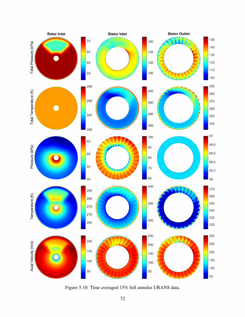
Figure 5.10: Time averaged 15% full annulus URANS data.

72

with the high peak at approximately 240◦ and 5% span and the low peak at approximately 170◦ and

5% span. Both the 7.5% and 15% data have a slight phase shift in the circumferential distortion

location from the stator inlet to the stator outlet of approximately 10◦.

Total Temperature

As can be seen in Figure 5.10, the total temperature profile at the inlet to the rotor inlet is

identical to the 7.5% data (Figure 5.9). The cause of this is the inlet total pressure profile in both

simulations was set as a boundary condition.

At the stator inlet, circumferential total temperature distortion is present . This shows that

total temperature distortion generation occurred in the rotor region. This generated total tempera-

ture distortion has a higher magnitude than the 7.5% data (Figure 5.9). However, as was previously

observed in the total temperature profiles, the shape of the generated total temperature distortion

for the 15% data has the same shape and phase as the 7.5% data. The same total temperature in-

crease near the hub caused by viscous shearing present in the 7.5% data is visible in the 15% data.

The magnitude and thickness of the region is the same for both simulations.

At the stator exit, the magnitude, shape and phase of the total temperature circumferential

distortion have changed minimally from the stator inlet profile (Figure 5.10). This was also ob-

served in the 7.5% data (Figure 5.9). The main difference in the 15% data from the 7.5% data

for this profile is the magnitude of this distortion is greater in the 15% data. The ‘saw tooth’ pat-

tern caused by the radial high total temperature near the shroud passing through the stator blades

observed in the 7.5% data is also present in the 15% data.

Static Pressure

As can be seen in Figure 5.10, the static pressure profile at the inlet to the rotor has circum-

ferential distortion present. The distortion has a 1 per-rev shape. In the 7.5% data, this circumfer-

ential distortion is less apparent due to it’s low magnitude (Figure 5.9). The same radial distortion,

caused by the hub impeding the flow, observed in the 7.5% data is also present in the 15% data.

At the stator inlet, 31 per-rev components dominate the profile. Radial variations are also

present with low pressure near the hub and high pressure near the shroud. This is consistent with

73

the 7.5% results (Figure 5.9). However, in the 7.5% data at the stator inlet, no static pressure

circumferential distortion was observed. In the 15% data (Figure 5.10), circumferential static

pressure distortion is visible apparent at the stator inlet. Upon, review of the 7.5% data, it is

possible that distortion is present for this profile. However, the 31 per-rev components make it

difficult to confirm this. In the 15% data, this distortion has a low pressure region at 135◦ and

a high pressure region at 240◦. These locations match the circumferential locations of the total

pressure distortion. It is difficult to identify the radial location of these regions due to the radial

variations and 31 per -rev components present in the profile.

At the stator outlet the static pressure is constant. This is identical to the 7.5% data and is

expected since this is a set outlet boundary condition.

Static Temperature

As can be seen in Figure 5.10, the static temperature profile at the rotor inlet contains

the 90◦ sector shape. A noticeable variation of this profile from the 7.5% data for this profile is

that there is an apparent skewing of the 90◦ sector in the 15% static temperature data at the rotor

inlet. This skewing is most prominent at approximately 30% span. This effect could be caused by

inconsistent work done by the downstream rotor. As can be seen in the total pressure rotor inlet

profile in Figure 5.10, as the rotor rotates through the total pressure distortion, it experiences rapid

changes in incoming total pressure. In this figure the rotor rotates cw. As a given rotor blade passes

from the 120◦ location to 150◦, the total pressure of the incoming air drastically decreases from 71

kPa to 63 kPa. The pressure side of the rotor blade encounters this rapid decrease in pressure first.

The result of this is the difference in pressure between the pressure and suction side of the blade

decreases in this region. The result of this is less work is done on the flow in this region.

In contrast to this, as the rotor blade passes through the 210◦ to 240◦ region, the total

pressure of the incoming air drastically increases from 63 kPa to 71 kPa. The result of this is the

pressure on the pressure side of the blade increases, increasing the pressure difference between the

suction and pressure sides of the blade. This results in more work being done on the flow in this

region. This inconsistent work done on the flow depending on rotor location causes inconsistent

flow effects that propagate upstream to the rotor inlet boundary.

74

At the stator inlet, the 15% data closely resembles the 7.5% data. The main difference

observed is the 15% data has more prominent static pressure distortion. The same trend is observed

at the stator outlet.

Axial Velocity

Finally, the axial velocity profiles are evaluated. As can be seen in Figure 5.10, the axial

velocity at the rotor inlet very closely mimics the inverse of the static temperature profile at the

rotor inlet. This was also observed in the 7.5% data for the same profile (Figure 5.9). The same

skewing effect observed in the static temperature profile is also present in the axial velocity profile.

This skewing effect was not apparent in the 7.5% data for axial velocity at the rotor inlet.

At the stator inlet, the inverse mimicking effect observed at the inlet, no longer holds true

(Figure 5.10). The cause of this is the presence of total temperature distortion at the stator inlet.

Before, it was acknowledged that the constant total temperature at the rotor inlet is the reasoning

for the inverse mimicking effect. Therefore, when distortion is present, the axial velocity and

static temperature do not inversely mimic one another. This is also observed for radial variations.

The static temperature has a noticeable low region nearest the hub. However, the axial velocity is

relatively uniform in the radial direction with the exception of the boundary layer present near the

shroud. Therefore, the axial velocity radial variations inversely mimic the total temperature profile

at the stator inlet.

At the stator outlet, the axial velocity profile is similar to the 7.5% data for the same profile

with the exception of the increased magnitude of the circumferential distortion.

Summary of Qualitative Analysis

From the qualitative analysis of the 7.5% and 15% flow fields, the following observations

were made.

1. Total pressure distortion is significantly reshaped through the rotor region for both data sets.

2. Total temperature distortion was generated in the rotor region for both data sets. The shape

of the generated distortion profile mimics the total pressure distortion profile at the same

75

place. However, the generated total temperature distortion is phase lagged approximately

10◦ ccw from the phase of the total pressure distortion profile.

3. Static temperature and axial velocity mimic each other inversely at the rotor inlet when total

temperature is constant.

5.2.3 Quantitative Distortion Transfer and Generation Comparison

Upon completing the qualitative analysis distortion transfer and generation, a Fourier anal-

ysis of the distortion transfer and generation was conducted. Distortion transfer is defined as the

change in total pressure distortion as it passes through the fan/compressor. Distortion generation

is defined as the generation of total temperature distortion as a constant total temperature pro-

file passes through the fan/compressor. The purpose of the Fourier analysis is to determine if

the qualitative observations can be identified quantitatively. The analysis follows the same form

demonstrated in Section 5.1.This section discusses this analysis.

Distortion Magnitude

Figures 5.11, 5.12 and 5.13 give information about the total pressure and total temperature

distortion magnitude. Figure 5.11 shows the time-averaged and radial-averaged total pressure and

total temperature profiles for both the 7.5% and 15% data sets. These plots are primarily included

as a reference to aid in the interpretation of the quantitative analysis. The data has been radial-

averaged since the circumferential distortion is of primary concern over radial distortion. Plots

of the profiles at 25%, 50%, 75% and 90% span have been included as supplemental results in

Appendix B.

Figures 5.12 and 5.13 show the modal amplitudes of the radial and time-averaged total

pressure and total temperature for the 7.5% and 15% data sets respectively. 8 modes have been

plotted in these figure as these are sufficient for the modal analysis conducted. All modes greater

than 8, with the exception of modes 20 and 31 (the fundamental frequencies of the rotor and

stator respectively), have an amplitude less than 0.25 kPa and 0.25 K for total pressure and total

temperature respectively. This amount was identified as relatively insignificant in Section 5.1.2.

76

(a) 7.5% distortion transfer and generation.

(b) 15% distortion transfer and generation.

Figure 5.11: Comparison of the radial-averaged distortion transfer and generation for the 7.5%and 15% full annulus URANS data.

77

(a) Distortion transfer. (b) Distortion generation.

Figure 5.12: Fourier modal amplitudes applied to distortion transfer and generation for the radialand time-averaged 7.5% full annulus URANS data for the rotor inlet, stator inlet and stator outlet.

(a) Distortion transfer. (b) Distortion generation.

Figure 5.13: Fourier modal amplitudes applied to distortion transfer and generation for the radialand time-averaged 15% full annulus URANS data for the rotor inlet, stator inlet and stator outlet.

78

Table 5.2: Total amplitude of distortion transfer andgeneration for the radial and time-averaged

7.5% and 15% full annulus data.

Total Pressure (kPa) Total Temperature (K)Location 7.5% 15% 7.5% 15%Rotor In 3.82 8.63 0.01 0.01Stator In 5.80 12.0 5.10 12.6

Stator Out 5.43 12.2 4.69 11.9

The distortion transfer through the rotor region is analyzed first. As can be seen in Figure

5.12a, each of the modal amplitudes plotted increase from the rotor inlet (red) to the stator inlet

(blue). Specifically, mode 1 increases from 1.47 kPa to 2.17 kPa (0.7 kPa or 48%), mode 2 in-

creases from 1.0 kPa to 1.78 kPa (0.78 kPa or 78%) and mode 3 increases from 0.47 kPa to 0.84

kPa (0.37 kPa 79%). This increase of amplitude across all modes signifies an increase in mag-

nitude. To quantify this overall increase in total pressure distortion, the total amplitude is used.

As can be seen in Table 5.2, the total amplitude of the total pressure distortion for the 7.5% data

increases from 3.82 kPa at the rotor inlet to 5.8 kPa at the stator inlet (1.98 kPa). Therefore, the

magnitude of the distortion has increased by 52%.

An inspection of Figure 5.11a confirms this deduction from the quantitative data. In this

figure, it is observed that the magnitude of the distortion at the rotor inlet (red) increases as it passes

through the rotor region to the stator inlet (blue). Therefore, the quantitative analysis accurately

captured the increase in magnitude.

The 15% data experiences the same increase in magnitude through the rotor region. As can

be seen in Figure 5.13a, each of the modes plotted increase in amplitude from the rotor inlet to

the stator inlet. Specifically, mode 1 increases from 3.24 kPa to 4.35 kPa (34%), mode 2 increases

from 2.25 kPa to 3.71 kPa (65%) and mode 3 increases from 1.09 kPa to 1.71 kPa (57%). As can

be seen in Table 5.2, the total amplitude increases from 8.63 kPa to 12.0 kPa (39%). This increase

in amplitude is verified by visual inspection of Figure 5.11b.

The increase in magnitude observed by both the 7.5% and 15% data through the rotor region

was previously expected as similar trends were observed by Yao and Gorrell [6] [14]. The cause of

this increase in distortion is related to how the rotor works on the flow. As the rotor rotates through

79

the total pressure distortion, it experiences rapid changes in incoming total pressure. This can be

illustrated with Figure 5.11b. In this figure the rotor’s direction of rotation is from left to right. As

a given rotor blade passes from the 120◦ location to 150◦, the total pressure of the incoming air

drastically decreases from 71 kPa to 63 kPa. The pressure side of the rotor blade encounters this

rapid decrease in pressure first. The result of this is the difference in pressure between the pressure

and suction side of the blade decreases in this region. The result of this is less work is done on the

flow in this region.

In contrast to this, as the rotor blade passes through the 210◦ to 240◦ region, the total

pressure of the incoming air drastically increases from 63 kPa to 71 kPa. The result of this is the

pressure on the pressure side of the blade increases, increasing the pressure difference between the

suction and pressure sides of the blade. This results in more work being done on the flow in this

region. This inconsistent work done on the flow depending on rotor location adds to the incoming

total pressure distortion, increasing the magnitude of the total pressure distortion.

A unique observation from the quantitative analysis, not previously shown in any other

study, is that the lower magnitude inlet distortion (7.5% data) experienced a larger percent increase

in magnitude than the higher magnitude inlet distortion (15% data) through the rotor region. To

clarify, the 7.5% data experienced an increased magnitude of 52% through the rotor region, while

the 15% data experienced an increased magnitude of 39%. The cause of this trend is likely con-

nected to the inconsistent work done on the flow.

Next, the distortion transfer through the stator region is analyzed. As can be seen in Figure

5.12a, each of the modal amplitudes plotted decrease from the stator inlet (blue) to the stator outlet

(green). Table 5.2 shows that the total amplitude decreases from 5.80 kPa at the stator inlet to 5.43

kPa at the stator outlet. This is a decrease of 0.37 kPa or 6.4%. This decrease in amplitude is small

enough that it is difficult to deduce strictly from a qualitative analysis of Figure 5.11a. Especially,

due to the 31 per-rev perturbations present at the stator outlet.

The 15% data shows a different trend through the stator region. As can be seen in Figure

5.13a, modes 1-4 increase from the stator inlet to the stator outlet while modes 5-8 decrease. Table

5.2 shows that the magnitude of the profile actually increases through the stator region from 12.0

kPa at the stator inlet to 12.2 kPa at the stator outlet. This is an increase of 0.2 kPa or an increase

80

of 1.7%. This change is also small enough that it is difficult to deduce strictly from a qualitative

analysis of Figure 5.11b.

An interesting observation is that the magnitude of the total pressure distortion through the

stator region decreased in the 7.5% data and increased in the 15% data. An analysis of the fan as

a whole brings insight into this observation. As can be seen in Table 5.2, the total amplitude of

the total pressure distortion for the 7.5% data increases from 3.82 kPa at the rotor inlet to the 5.43

kPa at the stator outlet. This is an increase of 1.61 kPa or 42.2%. The 15% data increases from

8.63 kPa to 12.2 kPa. This is an increase of 3.57 kPa or 41.4%. Therefore, the percent increase in

total pressure distortion through the fan is different by only 0.8% between the two data sets. This

signifies that the percent increase in total pressure distortion transfer may be independent of the

magnitude of the distortion at the inlet. In other words, a 10% 90◦ total pressure distortion profile

may also experience a percent increase in total pressure distortion across the fan of approximately

42%. This study only used two distortion profiles, therefore this is insufficient data points to

warrant statistical significance. However, this observation is worth further investigation in future

studies.

Next the total temperature distortion generation is analyzed. As can be seen in Figure

5.12b, the 7.5% data experiences an increase in each of the modal amplitudes through the rotor

region. Table 5.2 shows that this increase is from 0.01 K at the rotor inlet to 5.10 K at the stator

inlet. Each of the modal amplitudes then decrease through the stator region. Table 5.2 shows that

this decrease is from 5.10 K at the rotor inlet to 4.69 K at the stator inlet. This is a decrease of 0.41

K or 8%.

The 15% data also experiences an increase of total temperature magnitude through the rotor

region. As can be seen in Figure 5.13b, each of the modal amplitudes increase form the rotor inlet

to the stator inlet. Table 5.2 shows that this increase is from 0.01 K at the rotor inlet to 12.6 K at

the stator inlet. Each of the modal amplitudes then decrease through the stator region. Table 5.2

shows that this decrease is from 12.6 K at the rotor inlet to 11.9 K at the stator inlet. This is a

decrease of 0.7 K or 18%.

This analysis of the total temperature distortion generation shows that the most change

is experienced through the rotor region. The reason for this is the total temperature distortion

generation is caused by the same mechanism that caused the increase in total pressure distortion.

81

This is that the amount of work done by the rotor is circumferentially dependent. Since the amount

of work done by the rotor is circumferentially dependent, so is the total temperature rise, generating

distortion. Through the stator region, there is no work done on the flow so decreases in total

temperature distortion magnitude are primarily caused by the dissipation.

In summary, the following insights on distortion transfer and generation magnitude were

deduced from the Fourier analysis:

1. Total pressure distortion increases in magnitude as it passes through the rotor. This increase

is observed in all modal amplitudes and the total amplitude for both data sets. The mech-

anism causing this increase in distortion magnitude is inconsistent work done by the rotor

depending on circumferential location.

2. Total temperature distortion is generated as the flow passes through the rotor. This increase is

observed in all modal amplitudes and the total amplitude for both data sets. The mechanism

that causes this is the same as the mechanism that increases total pressure distortion.

3. The increase in total pressure distortion magnitude across the entire domain was similar for

both the 7.5% data and the 15% data with a difference of only 0.8%. This shows that the

percent increase in distortion across the entire fan may be independent of the magnitude of

the incoming distortion.

4. Total temperature distortion decreases through the stator region for both data sets. The reason

for this is no work is done on the flow by the rotor. Therefore, decreases in distortion

magnitude are caused by dissipation.

Distortion Shape

Distortion shape is a quantitative description of the shape of a given distortion profile. Some

qualitative examples of distortion shape are sinusoidal, 1 per-rev and 90◦ sector. This parameter is

crucial to understanding how the shape of the distortion profile is altered as it passes though a rotor

or stator region. The shape of a profile also has a direct effect on the performance downstream

fan/compressor. The same figures as were used for the distortion magnitude analysis will be used

for the distortion shape analysis. These are Figures 5.11, 5.12 and 5.13. Contour plots of the

82

distortion profiles overlaid on one another have also been provided in Appendix B for further

visualization of distortion shape change.

First, the total pressure shape change through the rotor region is evaluated for the 7.5%

data. As can be seen in Figure 5.12, mode 1 increases from the rotor inlet to the stator inlet by

48%, mode 2 by 78% and mode 3 by 79%. As was demonstrated in Section 5.1.2, this inconsistent

percent change in modal amplitudes signifies a shape change. Specifically, the 2 per-rev and 3

per-rev components of the profile have become more prominent. This can be visualized in Figure

5.11a. At the stator inlet there is a local minimum and maximum at 150◦ and 240◦ respectively.

This period of 90◦ between minimum and maximum is the same period of between minimum and

maximum for mode 2.

The same trend is observed for the 15% data. As can be seen in Figure 5.13, mode 1

increases from the rotor inlet to the stator inlet by 34%, mode 2 by 65% and mode 3 by 57%.

Therefore, one again, mode 2 has become more prominent in the stator inlet profile. To understand

this qualitatively, Figure 5.11b can be evaluated. In this figure, it is observed that the minimum

and maximum peaks are located at 135◦ and 225◦ respectively. This is a phase shift of 90◦. Mode

2 of the Fourier series also has a min-to-max phase shift of 90◦. The manifestation of this is the

2 per-rev component is more prominent in the stator inlet profiles. The cause of the reshaping

through the rotor region for both simulations is related to the inconsistent work done on the flow.

The rotor does less work on the flow between 120◦ and 150◦. This results in a lower pressure rise

in this range. The rotor does more work on the flow between 210◦ and 240◦. This is the same

mechanism that increases the distortion magnitude through the rotor region.

Next, the total pressure distortion shape change through the stator region is analyzed. As

can be seen in Figure 5.12, each of the modal amplitudes decrease through the stator region by

approximately 4%. Specifically, mode 1 decreases from the 2.17 kPa at the stator inlet to 2.10 kPa

at the stator outlet (0.07 kPa or 3.2%), mode 2 decreases from 1.78 kPa to 1.72 kPa (0.06 kPa or

3.5%) and mode 3 decreases from 0.84 kPa t 0.78 kPa (0.06 kPa or 7.1%). The similar percent

decrease in modal amplitude for modes 1 and 2 is significant because it quantitatively shows that

the shape of the total pressure distortion remains mostly unchanged through the stator region. The

percent decrease of mode 3 is higher than modes 1 and 2. This signifies that the shape of the profile

83

has changed some. However, since the modal amplitudes of modes 1 and 2 are significantly higher

than mode 3 (more than double) these are more significant for describing the shape of the profile.

In the 15% data, instead of decreasing from stator inlet to stator outlet, the modal ampli-

tudes slightly increase. As can be seen in Figure 5.13, each of the modes increase through the

stator region by approximately 4%. Specifically, mode 1 increases by 9.8%, mode 2 by 5.4% and

mode 3 by 12.3%. Once again, each of these values are similar to each other, signifying that there

is minimal shape change through the stator region.

An analysis of the total temperature distortion shape change through the rotor and stator

regions yields the same trends as were observed for the total pressure distortion shape change. As

can be seen in Figures 5.12 and 5.13, in both the 7.5% and 15% data sets, the total temperature

modal amplitudes are zero at the rotor inlet and non-zero at the stator inlet. This signifies a sig-

nificant shape change in both data sets across the rotor region. The cause of this shape change

is the same mechanism that causes total temperature distortion generation. This mechanism is

inconsistent rotor work based on circumferential location.

Through the stator region, the same consistent percent change in modal amplitudes is ob-

served for total temperature as was observed for total pressure. As can be seen in Figures 5.12

and 5.13, each of the modal amplitudes decrease by approximately 4% for both the 7.5% and 15%

data. Therefore, there is minimal shape change through the stator region. The reason for this is

there is no work done on the flow in the stator region.

5.2.4 Performance Parameters

The performance parameters for the 7.5% and 15% distortion simulations have been tabu-

lated in Table 5.3. These results only represent a single operating condition near design [2]. The

subscripts 1, 2 and f represent the fan inlet, fan outlet and the fan as a whole respectively. π f , τ f

and η f represent the total pressure ratio, total temperature ratio and efficiency respectively. Fan

efficiency was calculated using the polytropic efficiency equation (Equation 5.1).

η f =π

γ−1γ

f −1

τ f −1(5.1)

84

Table 5.3: Comparison of thefan performance values for

the 7.5% and 15% fullannulus URANS

simulaions.

Parameter 7.5% 15%Pt,1 (kPa) 70.37 69.59Tt,1 (K) 288.2 288.2Pt,2 (kPa) 131.21 130.67Tt,2 (K) 353.8 354.7π f 1.865 1.878τ f 1.228 1.231η f 0.856 0.855

As can be seen in the table, the performance values across the simulations have minimal

differences. There is less than 0.7% difference in the pressure ratio, less than 0.25% difference in

the temperature ratio and a 0.01% difference in the efficiency. This percent difference between the

simulations is less than the resolution of most experimental measurement methods. Therefore the

performance values are effectively identical. This is a very surprising result as the 15% distortion

was shown to have more than double the total amplitude of the 7.5% distortion profile. Even

with this significant increase in amplitude, the two simulations performed effectively identically.

This suggests that the magnitude of a given inlet distortion profile affects the performance of a

single stage up to some critical magnitude, beyond which the increase of distortion magnitude has

minimal additional effect on stage performance. It is worth mentioning that this is strictly for the

operating point simulated in these data sets. As the operating point approaches stall, it is likely

that the 15% distortion simulation would begin to stall before the 7.5% distortion simulation.

It is also worth mentioning that the similar fan performance values do not imply that the

overall fan/compression system performance will be the same for both of these inlet distortion

profiles. The total pressure distortion total amplitude of the 15% data exiting the fan (12.2 kPa)

is more than double the 7.5% data exiting the fan (5.43 kPa). Due to this, it is expected that the

higher total amplitude of the 15% data will have more of an adverse effect on the downstream

compressor. However, in the single stage fan, the affect on performance is essentially identical.

85

5.2.5 Discussion of 7.5% and 15% Distortion Comparison Results

In summary, the following observations were made during the qualitative and quantitative

analysis of the 7.5% and 15% full annulus URANS data sets:

1. The total pressure and total temperature distortion increased in magnitude and changed shape

through the rotor region. The total pressure total amplitude increased by 52% and 39%

through the rotor region for the 7.5% and 15% simulations respectively. Total temperature

total amplitude increased from 0.01 K to 5.10 K and 12.6 K through the rotor region for the

7.5% and 15% simulations respectively. The mechanism driving this is inconsistent work

done by the rotor based on circumferential location.

2. The total pressure and total temperature distortion magnitude and shape changed minimally

through the stator region. The reason for this is no work is done on the flow by the stator

blades.

3. The quantitative Fourier analysis was capable of capturing the distortion magnitude and

shape change observations made during the qualitative analysis. The Fourier analysis also

allowed for the distortion transfer and generation to be analyzed without blade row effects

and unbiased.

4. The increase in total pressure distortion magnitude across the entire domain was similar for

both the 7.5% data and the 15% data with a difference of only 0.8%. This shows that the

percent increase in distortion across the entire fan may be independent of the magnitude of

the incoming distortion.

5. Fan performance values were nearly identical across the data sets. This suggests that the

magnitude of a given inlet distortion profile affects the performance of a single stage up to

some critical point, beyond which the increase of distortion magnitude has minimal addi-

tional effect on stage performance.

Next, a quantitative analysis of the HB results will be conducted to evaluate if the same

trends observed for the full annulus URANS results discussed in this section are capable of being

captured by the HB solver.

86

5.3 Harmonic Balance Results

The harmonic balance results were compared against the baseline 7.5% full annulus URANS

simulation data to evaluate the HB solvers ability to capture distortion transfer and generation. This

section discusses the evaluation of three HB simulations. These are the HB(5-0-0), HB(3-1-1) and

HB(2-2-2) simulations. For a discussion of why these mode combinations were chosen, see Sec-

tion 4.4.5. The computational cost of each simulation is compared to determine solver viability.

Each of the simulations were evaluated using the Fourier descriptors. Performance values were

also used to determine how these were captured by each of the HB simulations.

5.3.1 Computational Cost Comparison

The computational cost requirements of each of the HB simulations were evaluated and

compared against the 7.5% full annulus URANS requirements. The computational costs of the

7.5% full annulus URANS simulation and the HB simulations have been tabulated in Table 5.4.

The values included in this table are file size, effective mesh, iterations, wall time, processors and

CPU hours (CPH). The definition and derivation of each of these parameters are follows:

1. The file size represents the simulation file size. This represents both the grid and the solution.

For the full annulus simulation, the file size is approximately equal to a single time accurate

solution for the full computational domain. For the HB simulations, the file size represents

the full solution for any physical time.

2. The effective mesh is calculated for the HB simulations using Equation 4.6. For the full

annulus simulation the effective mesh is simply the total cell count of the simulation.

3. The iterations represent the number of iterations required to converge the simulation. Con-

vergence was considered achieved when the inlet mass flow and outlet mass flow matched

and stopped fluctuating irregularly. Minor periodic fluctuations were still present in the mass

flow since time accurate simulations always fluctuate to some extent. The reason for this is

turbomachinery flow is inherently periodic. The residuals were also analyzed to ensure that

these also were no longer fluctuating.

4. The wall time represents the actual time required to achieve a converged solution.

87

Table 5.4: Comparison of the convergence computational cost requirements forthe 7.5% full annulus URANS simulation and the HB simulations.

Parameter 7.5% Full Ann HB(5-0-0) HB(3-1-1) HB(2-2-2)File Size (GB) 150 16 27 32Effective Mesh (cells) 293 M 116.6 M 693 M 3,025 MIterations 400,000 29,000 28,500 30,500Wall Time (days) 18.5 4.8 5.3 6.5Processors 2,400 1,280 1,280 1,920CPH (hours) 1.06 M 0.147 M 0.163 M 0.297 M

5. The number of processors represents how many processors were utilized to achieve a con-

verged solution. All simulations were run on the Department of Defense (DoD) High Per-

formance Computing (HPC) systems. The full annulus simulation was run on the Lightning

machine and all HB simulations were run of the Spirit machine.

6. The CPH represents the computational time required to achieve a converged solution and is

calculated by multiplying the wall time by the number of processors used.

As can be seen in Table 5.4, the full annulus simulation file size is more than 9 times larger

than the HB(5-0-0) simulation and more than 4.5 times larger than the HB(2-2-2) simulation. Due

to the large file size of the full annulus simulation, this simulation required a minimum of 1,000

processors to begin iterating. The optimum number of processors was 2,400. Running on more

than 2,400 processors resulted in longer queue times with minimal decrease in iteration solution

time (due to increased communication time). Running on fewer than 2,400 processors greatly

increases iteration solution time. 2,400 processors is an expensive resource requirement and ads to

the true time requirement for achieving such a simulation. The reason for this is greater resource

requests have longer queue times. The full annulus simulations run for this study were submitted

approximately 4 times before completing convergence and time accurate extraction. Each time the

simulation was submitted to the HPC system, there was an average queue time of approximately

3 days. This adds up to almost 2 weeks of queue time. This total queue time will be highly

variable depending on the type of queue system used, the number of processors on a system and

many other factors. However, the trend of larger processor requests resulting in longer queue times

88

should hold across the majority of HPC systems. Therefore, the reduced processor requirements

of the HB simulations across the board, increases the appeal of the HB solver.

The effective mesh sizes of the HB simulations give insight into the how mode selection

effects CPH. As can be seen in Table 5.4, The effective mesh of the HB(5-0-0) simulation is the

smallest at 116.6 M cells and the HB(2-2-2) simulation has the largest effective mesh at 3.025 B

cells. A trend is observed between effective mesh and CPH. The HB(5-0-0) simulation required

0.147 M hours while the HB(2-2-2) simulation required almost twice the CPH at 0.297 M hours.

The HB(3-1-1) simulation was in-between with a CPH of 0.163 M hours. As the effective mesh

increases the required CPH also increases in a polynomial manner.

As can be seen in Table 5.4, the number of iterations required to achieve a converged

simulation is very similar across all HB simulations. This suggests that the number of iterations

required is independent of the effective mesh. The full annulus simulation required more than an

order of magnitude more iterations than the HB simulations. This is due to the fact that the full

annulus simulation is using an unsteady, time accurate solver. These solvers require many iterations

to resolve unsteady behavior. Since the HB solver operates in the frequency domain, steady state

solvers are used, greatly reducing the number of iterations required to achieve convergence.

In summary, the HB solver is significantly cheaper to achieve convergence in terms of

file size, processors required, wall time and the total computational cost. Also, HB simulations

show a correlation between effective mesh and the CPH required for convergence. However, the

number of iterations required to achieve convergence is independent of the effective mesh. These

observations are significant because they provide initial viability of the HB solver. The significantly

cheaper computational costs are attractive aspects of the HB solver.

5.3.2 Distortion Transfer and Generation Comparison

This section outlines the evaluation of the ability of the HB solve to capture distortion

transfer and generation. Each of the HB simulations are compared against the 7.5% full annulus

URANS simulation and each other. The HB simulations are evaluated in the following order:

HB(5-0-0), HB(3-1-1) and HB(2-2-2).

89

Figure 5.14: Comparison of the radial time-averaged total pressure and total temperature profilesat the rotor inlet, stator inlet and stator outlet for the HB(5-0-0) and 7.5% full annulus data.

Harmonic Balance 5-0-0

The HB(5-0-0) simulation is evaluated first. The radial and time averaged data for total

pressure and total temperature have been plotted for both the HB(5-0-0) simulation and the 7.5%

full annulus URANS simulation in Figure 5.14. The modal amplitudes for the same data have also

been plotted in Figure 5.15.

As can be seen in Figure 5.14, the HB approximation of the rotor inlet total pressure dis-

tortion profile matches the general shape of the full annulus profile, but with apparent cyclical

behavior caused by the lower order approximation of the flow field. At the stator inlet, the HB data

matches the full annulus data better than at the inlet. This is true for both total pressure and total

temperature. At the stator outlet, the best match is achieved. The goodness of the profile match

can be quantified by viewing the modal amplitudes (Figure 5.15). The modal amplitudes are sig-

nificant because they give information about the shape and magnitude of the distortion profile. The

HB(5-0-0) simulation is successful in matching the total pressure modal amplitude trends of the

full annulus simulation at the rotor inlet. The HB modes overestimate the full annulus data for

modes 1, 2, 3 and 5 by 0.05 kPa, 0.08 kPa, 0.03 kPa and 0.1 kPa respectively. These values are

90

Figure 5.15: Comparison of the radial time-averaged total pressure and total temperature modalamplitudes at the rotor inlet, stator inlet and stator outlet for the HB(5-0-0) and 7.5% full annulusdata.

relatively low considering the maximum modal amplitude at the rotor inlet is 1.47 kPa. All modal

amplitudes higher than 5 are 0. This is due to the HB data only approximating the distortion profile

with 5 modes. Therefore, modes higher than 5 do not and cannot exist.

How well the total pressure distortion magnitudes match at the rotor inlet can be evaluated

by analyzing the total amplitude (Table 5.5). The significance of the total amplitude is that it is

a measure of the total amount of distortion present in a profile. The total amplitude is calculated

by summing all modal amplitudes (Equation 4.8). The 7.5% full annulus data has a total pressure

distortion total amplitude at the rotor inlet of 3.82 kPa. The HB(5-0-0) data under-estimates this

total amplitude by 10.5% with a value of 3.42 kPa. This underestimation is due to the lack of

91

Table 5.5: Total amplitude of distortion transfer and generation for theradial and time-averaged HB(5-0-0) and 7.5% full annulus data.

Total Pressure (kPa) Total Temperature (K)Location 7.5% HB(5-0-0) % Diff 7.5% HB(5-0-0) % DiffRotor In 3.82 3.42 10.5% 0.01 0.16 N/AStator In 5.80 5.53 4.7% 5.10 4.54 10.8%

Stator Out 5.43 5.39 0.7% 4.69 4.24 9.6%

modes above mode 5. Therefore 10.5% of the total pressure distortion present at the rotor inlet is

not captured when 5 modes are used to approximate the distortion.

The total pressure distortion profile continues to match well at the stator inlet between the

7.5% and HB(5-0-0) data. Figure 5.15 shows that modes 1-5 have the same trends across both

simulations. The largest difference between the two simulations is mode 1 with the HB(5-0-0)

simulation over-estimating by 0.2 kPa. This is relatively small given the mode 1 amplitude is 2.17

kPa for the 7.5% data. Table 5.5 shows that the magnitude of the HB(5-0-0) total pressure distortion

at the stator inlet under-estimates the 7.5% data by 4.7%. Therefore, 95.3% of the magnitude of

the total pressure distortion is being captured at the stator inlet. This is better than the percent error

of 10.5% at the rotor inlet. This trend continues across the HB simulations and will therefore be

discussed later.

The total pressure distortion also matches well at the stator outlet. As can be seen in Figure

5.15, the trends of modes 1-5 match between the 7.5% and HB(5-0-0) data. The largest difference

is in mode 1 with the HB(5-0-0) simulation over-estimating by 0.23 kPa. Mode 1 has an amplitude

of 2.1 kPa for the 7.5% data. Table 5.5 shows that the magnitude of the HB(5-0-0) total pressure

distortion at the stator outlet under-estimates the 7.5% data by 0.7%. Therefore, 99.3% of the

magnitude of the total pressure distortion is being captured at the stator outlet.

A surprising observation is that the total amplitudes matched the best at the stator outlet.

A qualitative assessment of the time averaged data (Figure 5.14) agrees that the HB(5-0-0) data

matches the 7.5% data the best at the stator outlet. It was presumed that the errors in the approxi-

mation at the inlet would propagate through the rotor and stator regions, amplifying the error. The

reason that the outlet matches the best is likely due to how the profile has reshaped. At the rotor

inlet modes 1, 2 and 3 dominate however the higher order modes are still of great significance

92

especially in capturing the severe gradients present at 135◦ and 225◦. As the profile moves through

the rotor, the lower order modes are amplified more than the higher order modes. This was ob-

served and discussed in length in Section 5.2.3. This makes the lower order modes a larger fraction

of the total amplitude. Also, as the profile passes through the fan, the severe gradients observed

at the rotor inlet dissipate. Higher order modes are critical in capturing sever gradients, because

higher order modes contain more severe gradients. As the profile dissipates, the severe gradients

resolve first, resulting in the attenuation of higher order modes. As the lower order modes begin

to dominate the total amplitude, the HB(5-0-0) simulation, which can only capture the lower order

modes, is able to represent a larger fraction of the total amplitude.

The analysis of the total temperature distortion generation results in the same trends as were

observed with the total pressure analysis. A unique observation to the total temperature analysis is

at the rotor inlet. As can be seen in Figure 5.15, the total temperature modal amplitudes at the rotor

inlet of the 7.5% data are zero. However, in the HB simulation there is distortion present. This is

due to an assumption made when setting up the HB wake specification boundary condition. It was

assumed that the static pressure distortion was zero when in reality minor distortion was present as

was shown in Section 5.2. The lack of this pressure distortion in the wake specification presented

itself as minor total temperature distortion. The total amplitude of this total temperature distortion

is 0.16 K (Table 5.5). This is still relatively low when compared to the 7.5% total amplitudes of the

total temperature at the stator inlet and the stator outlet, which are 5.10 K and 4.69 K respectively.

The total temperature distortion also matched the best at the stator outlet with a total am-

plitude percent difference of 9.6% below the 7.5% data. This match is not as good as the total

pressure percent difference.


Next, the HB(3-1-1) simulation is evaluated. The same variables plotted in Figures 5.14 and

5.15 have been plotted for the HB(3-1-1) data and the 7.5% full annulus URANS data in Figures

5.16 and 5.17. The total amplitudes of the HB(3-1-1) data and the 7.5% full annulus URANS data

have been plotted in Table 5.6. Compared to the HB(5-0-0) versus 7.5% full annulus comparison,

the following observations can be made.

93



Stator Out 5.43 4.98 8.3% 4.69 3.78 19.4%

1. The HB(3-1-1) modal amplitudes match the trends of the 7.5% data (Figures 5.17 and

5.16). As was observed with the HB(5-0-0) data, The HB(3-1-1) modal amplitudes that exist

(modes 1-3) overestimate the 7.5% modal amplitudes (with the exception of total pressure

mode 3 at the stator inlet and outlet). The average over-estimation of the modal amplitude

1-3 is 0.6 kPa for total pressure and 0.12 K for total temperature.

2. Due to the fewer modes for approximating the inlet distortion profile, the total amplitudes

of the HB(3-1-1) data do not match the 7.5% data as well as the HB(5-0-0) data. As can

be seen in Table 5.6, the total pressure total amplitude percent differences are 18.1%, 11.7%

and 8.3% for the rotor inlet stator inlet and stator outlet respectively. The same variables for

the HB(5-0-0) data are 10.5%, 4.7% and 0.7% (Table 5.5), each of which are lower than their

HB(3-1-1) counterpart. As can be seen in Table 5.6, the total temperature total amplitude

percent differences are 20.0% and 19.4% for the stator inlet and stator outlet respectively.

The same variables for the HB(5-0-0) data are 10.8% and 9.6% (Table 5.5). The HB(5-0-0)

percent differences are lower than the HB(3-1-1) data for total temperature total amplitude.

3. Like the HB(5-0-0) simulation, the HB(3-1-1) simulation matches the 7.5% data the best

at the stator outlet. This is observed in Table 5.6. Here the lowest total amplitude percent

differences are at the stator outlet for both the total pressure and total temperature distortion

(8.3% and 19.4% respectively).


Next, the HB(2-2-2) simulation is evaluated. The same variables plotted in Figures 5.14 and

5.15 have been plotted for the HB(2-2-2) data and the 7.5% full annulus URANS data in Figures

94


5.18 and 5.19. The total amplitudes of the HB(2-2-2) data and the 7.5% full annulus URANS data

have been plotted in Table 5.7. Compared to the HB(5-0-0) versus 7.5% full annulus comparison

and the HB(3-1-1) versus 7.5% full annulus comparison, the following observations can be made.

1. The HB(2-2-2) modal amplitudes match the trends of the 7.5% data (Figure 5.19). As was

observed with the HB(5-0-0) and HB(3-1-1) data sets, The HB(2-2-2) modal amplitudes that

exist (modes 1 and 2) overestimate the 7.5% modal amplitudes(with the exception of total

temperature mode 2 at the stator inlet and outlet). The average over-estimation of the modal

amplitude 1-3 is 0.8 kPa for total pressure and 0.12 K for total temperature.

2. Due to the fewer modes for approximating the inlet distortion profile, the total amplitudes

of the HB(2-2-2) data do not match the 7.5% data as well as the HB(5-0-0) and HB(3-1-1)

data sets. As can be seen in Table 5.7, the total pressure total amplitude percent differences

are 30.9%, 23.1% and 20.0% for the rotor, inlet stator inlet and stator outlet respectively.

These values are all higher than the HB(5-0-0) and HB(3-1-1) counterparts (Tables 5.5 and

5.6). As can be seen in Table 5.7, the total temperature total amplitude percent differences

95


are 38.2% and 38.0% for the stator inlet and stator outlet respectively. These values are all

higher than the HB(5-0-0) and HB(3-1-1) counterparts (Tables 5.5 and 5.6).

3. Like the HB(5-0-0) and HB(3-1-1) data sets, the HB(2-2-2) simulation matches the 7.5%

data the best at the stator outlet. This is observed in Table 5.7. Here the lowest total amplitude

percent differences are at the stator outlet for both the total pressure and total temperature

distortion (20.0% and 39.0% respectively).

96




Stator Out 5.43 4.34 20.0% 4.69 2.91 38.0%

Summary of Fourier Analysis

The following observations and suggestions are made based on the analysis of the HB

simulations.

1. The HB solver’s ability to capture total pressure distortion transfer and total temperature

distortion generation is considered excellent. The HB(5-0-0) simulation matched the full

annulus URANS data for total pressure total amplitude at the stator exit with 0.7% error

and matched total temperature with 9.6% error. This is significant because the validation of

the HB solver provides a new tool for diffuser, fan and compressor designers that requires

97


less computational time. This allows for faster iteration turn-over resulting in more design

iterations possible and therefore more efficient and optimized designs.

2. The HB(5-0-0) simulation was able to match the distortion transfer and generation the best

across all profiles. This was deduced by evaluating that the total amplitudes of the HB(5-0-0)

simulation matched the best across all values with the exception of the total temperature at

the rotor inlet. Also, from the analysis conducted, the inclusion of modes in the rotor and

stator blade rows had no observable effect on the capture of distortion transfer and genera-

tion.

98

The significance of this observation is it provides insight into selecting mode combination

for an HB simulation. If the capture of distortion transfer and generation are of the most

importance, sufficient modes should be applied to the inlet condition and modes in the rotor

and stator region can be set to 0. From the results of this study, it is recommended that

approximately 90% of the total amplitude of the inlet distortion profile should be captured

by the HB representation in order to accurately capture distortion transfer and generation.

3. The HB data provided new insight into distortion transfer and generation. It was observed

that the modal amplitudes and total amplitudes match the best at the outlet condition. This

led to the observation that as the inlet profile passes through the rotor and stator regions, the

lower order modes become more dominant. This is due to the severe gradients at the inlet

dissipating more rapidly.

The significance of this observation is it demonstrates how new insights into the distortion

transfer and generation physics can be obtained by using Fourier methods to analyze distor-

tion.

4. Even if a mode is effectively non-existent in the inlet distortion profile, that mode can still

be generated as the profile passes through the rotor and stator region. This effect is most

obvious with total temperature generation where no modes existed at the inlet and all modes

plotted existed at the stator inlet and stator outlet (See Figures 5.15, 5.17 and 5.19). However,

the HB solver can only preserve and generate modes within the modes specified at the inlet.

For example, the HB(2-2-2) simulation cannot generate mode 3 amplitudes as these are not

calculated within the solver.

The significance of this observation is it provides further recommendations into selecting

mode combination for an HB simulation. Simply because a mode does not exist at the inlet

condition, this is not enough reason to exclude that mode from the mode combination.

5.3.3 Fan Performance Comparison

The performance values for the HB simulations were evaluated and compared against the

7.5% full annulus URANS performance values. The performance values of the 7.5% full annulus

99

Table 5.8: Comparison of the fan performance values for the 7.5%full annulus URANS simulation and the HB simulations.

Absolute Values

Parameter 7.5% Full Ann HB(5-0-0) HB(3-1-1) HB(2-2-2)Pt,1 (kPa) 70.37 70.79 70.76 70.75Tt,1 (K) 288.2 288.2 288.2 288.2Pt,2 (kPa) 131.21 130.88 131.35 131.51Tt,2 (K) 353.8 354.2 354.0 353.92π f 1.865 1.849 1.856 1.859τ f 1.228 1.229 1.228 1.228η f 0.856 0.838 0.846 0.849

Percent Difference From 7.5% Data

Parameter 7.5% Full Ann HB(5-0-0) HB(3-1-1) HB(2-2-2)Pt,1 N/A 0.6% 0.6% 0.5%Tt,1 N/A 0.0% 0.0% 0.0%Pt,2 N/A 0.3% 0.1% 0.2%Tt,2 N/A 0.1% 0.1% 0.0%π f N/A 0.9% 0.5% 0.3%τ f N/A 0.1% 0.0% 0.0%η f N/A 1.8% 1.0% 0.7%

URANS simulation and the HB simulations have been tabulated in Table 5.8. Each of these values

have been mass-flow and time-averaged. The subscripts 1, 2 and f represent the fan inlet, fan

outlet and the fan as a whole respectively. π f , τ f and η f represent the fan total pressure ratio, total

temperature ratio and efficiency respectively. Fan efficiency was calculated using the polytropic

efficiency equation (Equation 5.1).

As can be seen in Table 5.8, each of the temperature and pressure values match the 7.5%

full annulus values within 2% error. Each of the HB Pt,1 values slightly over estimated the full

annulus value by about 0.5%. The largest Pt,1 percent error was for the HB(5-0-0) with a percent

error of 0.59%. This is also the largest percent error across all total pressure and total temperature

values. Each of the Tt,1 values matched exactly, which is to be expected since this is a boundary

condition set by the user.

The HB Pt,2 values follow a trend that the more modes used to describe the inlet distortion

and the fewer modes used to describe the blade rows resulted in a lower Pt,2 value. This translates

100

to the fan pressure ratio. The HB(5-0-0) had the lowest pressure ratio, underestimating the full

annulus pressure ratio by 0.8%. The HB(3-1-1) simulation underestimated by 0.4% and the HB(2-

2-2) simulation underestimated by 0.3%. While the underestimations are relatively small, these

errors are amplified by the efficiency calculation. The HB(5-0-0) fan efficiency underestimates

the full annulus value by just over 2%. The HB(3-1-1) simulation underestimates by 1% and the

HB(2-2-2) matches the best, underestimating by 0.6%.

The trend observed across the performance parameters for the HB simulations suggests

that blade row interactions have an effect on total pressure ratio which consequently affects fan

efficiency significantly. Therefore, in order to more accurately capture total pressure ratio and

efficiency, it is necessary to include modes in the blade row calculations.

The performance matching of HB simulations is considered excellent. This is significant

because it validates that the HB solver can be used to capture fan performance in CFD for simula-

tions when total pressure distortion is present.

5.3.4 Discussion of Harmonic Balance Results

The HB solutions have been compared against the 7.5% full annulus URANS simulation to

evaluate the HB solver’s computational cost requirements, ability to capture distortion transfer and

generation and also the solver’s ability to capture fan performance when total pressure distortion

is present. From the analysis that was conducted, the following conclusions can be made.

1. The HB solver has significantly lower computational requirements and physical time re-

quirements. This was true for all HB simulations run for this study. The physical time

required to obtain a converged solution was one third the time required for the time-accurate

full annulus simulation. The number of processors required to run the HB simulations was

three-fourths to one-half the full annulus requirement. The total CPH was 5 to 7 times less

the CPH required for the full annulus simulation.

2. The larger the effective mesh size (Equation 4.6), the longer the HB simulation will take

to achieve convergence. The effective mesh size drastically increases with the inclusion of

additional modes.

101

3. The HB solver is capable of capturing distortion transfer and generation. The more modes

used to capture the inlet distortion profile, the more accurate the distortion transfer and gen-

eration predictions will be. The Inclusion of modes in the blade rows had no perceivable

affect (favorable or adverse) on the capture of distortion transfer and generation. To ad-

equately capture distortion transfer and generation, it is recommended that the number of

modes used to represent the inlet distortion profile should capture a minimum of 90% of the

total pressure total amplitude at the inlet to the domain.

4. The HB solver’s ability to capture fan performance is considered excellent. The inclusion of

modes in the blade row regions is recommended to more accurately predict fan performance.

A minimum of 1 mode per blade row is recommended.

5. An overall ideal HB mode recommendation can be given for the inlet boundary condition and

geometry used for this study. This recommendation is 3-2-1. 3 modes for the inlet condition

was demonstrated as being capable of capturing distortion transfer and generation. 2 modes

are recommended for the rotor region since the rotor blade row effects have a significant

impact on the downstream stator. 1 mode is recommended for the stator region since the

tight blade spacing for this geometry results in the stator region having an impact on the

upstream rotor region. A single mode should be sufficient to capture this.

As a whole, the HB solver is effective at reducing computational costs while still being

able to capture distortion transfer, generation and fan performance. This is significant because

it provides a new tool to fan/compressor designers and researchers. The great reduction in the

computational cost requirements of the HB solver, increases the total number of simulations that

can be run in a set time period. This is valuable as it allows for quicker turn around times and

therefore, more design iterations. The validation of the HB solver also gives more credibility to

the application of Fourier methods for analysis of distortion transfer and generation.

102

CHAPTER 6. CONCLUSIONS

The SAE-ARP 1420b descriptors were shown to be inadequate at capturing the majority

of distortion profiles. The descriptor for distortion magnitude, intensity, was only able to provide

meaningful information about the profile when there were clearly defined low distortion regions.

When high and low distortion existed, the intensity descriptor did not capture the high distortion,

only the low. The extent descriptor also failed to give meaningful information when both high and

low distortion was present. The SAE-ARP descriptors also have no ability to capture shape, phase

or severity.

In contrast, the Fourier descriptors were shown to capture distortion magnitude, shape,

severity and phase. The modal amplitude and total amplitude descriptors were able to describe the

magnitude of high and low distortion regardless of the profile shape. These descriptors also allow

for either a modal analysis or a more broad analysis of the entire profile to be conducted. The modal

amplitude and phase descriptors give detailed information about the shape of the profile. When

used in conjunction they can reconstruct the profile via the Fourier series. The modal amplitude

can be used to rapidly identify the dominant shape of the profile. The relative change in the modal

amplitudes and the modal phases from one location to another give information about profile shape

change. The Fourier descriptor for severity, total amplitude, was shown to give a single value to

describe the total amount of distortion present in a profile. The modal phase was shown to be able

to describe the translation rotation of the distortion profile.

This validation of the Fourier descriptors is significant for the following reasons. First, it

establishes a new set of quantitative values that capture more information and are more robust than

pre-existing descriptors. This sets the foundation for the development of more robust models that

are not limited to the engine they are designed for. It also allows for the development of predictive

models that can predict degradation of performance and changes in magnitude, shape, severity,

and phase on a stage-by-stage basis. Second, the Fourier distortion descriptors are not limited

103

to specific profile types. These descriptors can be used to qualitatively describe any conceivable

profile shape for any parameter. This gives the Fourier descriptors a wide range of possible appli-

cations. Finally, the increased information that these descriptors can quantify provides new ways

of analyzing distortion transfer and generation that will increase current understanding of these

phenomenon.

Next, full annulus URANS data was presented and analyzed qualitatively, quantitatively

(using the Fourier descriptors) and in terms of performance. The motivation for comparing the

7.5% and 15% data sets was to gain understanding on how adjusting the magnitude of distortion

profiles affects distortion transfer, generation and performance parameters. It was shown that the

total pressure and total temperature distortion increased in magnitude and changed shape through

the rotor region. The mechanism driving this is inconsistent work done by the rotor based on

circumferential location. In contrast, the total pressure and total temperature distortion magnitude

and shape changed minimally through the stator region. The reason for this is no work is done on

the flow by the stator blades.

The ability of the Fourier descriptors to quantitatively capture distortion magnitude and

shape change was demonstrated. The Fourier analysis also allowed for the distortion transfer and

generation to be analyzed without blade row effects and unbiased. The increase in total pressure

distortion magnitude across the entire domain was shown to be similar for both the 7.5% data

and the 15% data with a difference of only 0.8%. This demonstrates that the percent increase in

distortion across the entire fan may be independent of the magnitude of the incoming distortion.

Fan performance values were nearly identical across the data sets. This suggests that the magnitude

of a given inlet distortion profile affects the performance of a single stage up to some critical

point, beyond which the increase of distortion magnitude has minimal additional effect on stage

performance.

Finally the 7.5% full annulus URANS data was compared against the HB(5-0-0), HB(3-1-

1) and HB(2-2-2) simulations. The motivation was to evaluate the HB solver’s ability to capture

distortion transfer, generation and the degradation on performance caused by the presence of inlet

distortion. From this comparison it was determined that the HB solver has significantly lower

computational requirements and physical time requirements. This was true for all HB simulations

run for this study. The physical time required to obtain a converged solution was one third the time

104

required for the time-accurate full annulus simulation. The number of processors required to run

the HB simulations was three-fourths to one-half the full annulus requirement. The total CPH was

5 to 7 times less the CPH required for the full annulus simulation. It was also shown that larger the

effective mesh size, the longer the HB simulation took to achieve convergence. The effective mesh

size drastically increases with the inclusion of additional modes.

It was demonstrated that the HB solver is capable of capturing distortion transfer and gener-

ation. The more modes used to capture the inlet distortion profile, the more accurate the distortion

transfer and generation predictions will be. The inclusion of modes in the blade rows had no

perceivable affect (favorable or adverse) on the capture of distortion transfer and generation. To

adequately capture distortion transfer and generation, it is recommended that the number of modes

used to represent the inlet distortion profile should capture a minimum of 90% of the total pressure

total amplitude at the inlet to the domain. It was also shown that the HB solver’s ability to capture

fan performance is considered excellent. The inclusion of modes in the blade row regions is rec-

ommended to more accurately predict fan performance. A minimum of 1 mode per blade row is

recommended. From the results of the HB simulations, it was determined that the optimal mode

HB mode combination for the 90◦ sector total pressure inlet distortion profile applied to the rotor

4 geometry is 5-2-1.

The HB solver is effective at reducing computational costs while still being able to capture

distortion transfer, generation and fan performance. This is significant because it provides a new

tool to fan/compressor designers and researchers. The great reduction in the computational cost

requirements of the HB solver, increases the total number of simulations that can be run in a set

time period. This is valuable as it allows for quicker turn around times and therefore, more design

iterations. The validation of the HB solver also gives more credibility to the application of Fourier

methods for analysis of distortion transfer and generation.

6.1 Future Work

Promising directions for future work related to Fourier descriptors and the HB solver are

as follows:

105

1. The Fourier descriptors (modal phase, modal amplitude and total amplitude) were all intro-

duced in the current thesis. The potential of these descriptors to capture distortion transfer

and generation was investigated. However, much more work is to be done to investigate the

full potential of Fourier distortion descriptors. It is suggested that statistical and numerical

methods be applied to the Fourier descriptors to identify trends. As trends are identified,

models could be generated to predict these trends. These models could then be tested on

different mode distortion profiles, distortion magnitudes and geometries.

2. The Fourier descriptors were shown to be effective for stage-by-stage analysis. To further

investigate this, it would be valuable to apply the methods described in this thesis to mul-

tistage fans and compressors. New data sets are not necessary for this study. The Fourier

descriptors could be applied to existing data sets (CFD or experimental) to gain increased

understanding of distortion transfer and generation as well as the underlying physics.

3. It was observed that the percent increase in total amplitude across the rotor 4 fan was the

same for both the 7.5% and 15% distortion profiles. Additional research could be done to

investigate this trend and under what conditions it holds true.

4. It was observed that the doing work on the flow field increased the magnitudes of the total

pressure distortion and generated total temperature distortion. By this observation, it may

also be hypothesized that extracting work from the flow field may be able to reduce distor-

tion magnitude. Research could be done to investigate the effects of passing total pressure

distortion profiles through turbines. If turbines are capable of reducing distortion magnitude,

it may lead to the development of gas turbine engines with turbines prior to the fan intended

for powering auxiliary systems.

5. To further investigate the limitations of the HB solver, studies could be conducted using the

HB solver on multistage geometries, varying distortion profile shapes and different operating

conditions. Such a study could investigate the HB solver’s ability to capture stall.

6. The convergence of the 15% HB simulations were unsuccessful. More work could be done

to identify and remedy the issue. This data could then be analyzed and compared against the

106

15% full annulus URANS data in the same manner as the HB evaluation conducted in this

thesis.

107

REFERENCES

[1] Cousins, W. “History, philosophy, physics, and future directions of aircraft propulsion sys-tem/inlet integration.” In Proceedings of ASME Turbo Expo 2004. 1, 4, 5, 6, 8

[2] List, M. G., 2013. “Numerical quantification of interaction effects in a closely-coupleddiffuser-fan system.” Ph.d. dissertation, University of Cincinnati, Cincinnati, OH, Decem-ber. 1, 8, 9, 17, 18, 20, 21, 84

[3] Pearson, H., and McKenzie, A. B., 1959. “Wakes in axial compressors.” Journal of the RoyalAeronautical Society, 63, July. 1, 8

[4] Reid, C., 1969. “The response of axial flow compressors to intake flow distortion.” ASME(69–GT–29). 1, 8, 47

[5] Hynes, T. P., and Greitzer, E. M., 1987. “A method for assessing effects of circumferentialflow distortion on compressor stability.” Journal of Turbomachinery, 109(—), pp. 371–379.1, 8, 47

[6] Yao, J., Gorrell, S. E., and Wadia, A. R., 2010. “High-fidelity numerical analysis of per-rev-type inlet distortion transfer in multistage fans–part i: Simulations with selected blade rows.”Journal of Turbomachinery, 132(041014). 1, 2, 13, 18, 47, 79

[7] Howell, K. B., 2001. Principles of Fourier Analysis. Textbooks in Mathematics Series.Chapman and Hall/CRC, Oxford, UK. 2, 17, 43

[8] SAE, 2002. Aerospace Recommended Practice, Rev. B. The American Society of AutomotiveEngineers, Warrendale, PA. 3, 6, 42, 49

[9] Nessler, C. A., Copenhaver, W. W., and List, M. G., 2013. “Serpentine Diffuser Performancewith Emphasis on Future Introduction to a Transonic Fan.” AIAA Paper 2013-0219. 4, 21

[10] Sanders, D. D., and List, M. G., 2013. “CFD Performance Predictions of a Serpentine Dif-fuser Configuration in an Annular Cascade Facility.” AIAA Paper 2013-0220. 4, 21

[11] Campbell, A., 1981. “An investigation of distortion indices for prediction of stalling behaviorin aircraft gas turbine engines.” M.s., Virginia Polythechnic Institute and State University. 6

[12] He, L., 2010. “Fourier methods for turbomachinery applications.” Progress in AerospaceSciences, 36, June, pp. 329–341. 10, 12

[13] Hah, C., Rabe, D. C., Sullivan, T. J., and Wadia, A. R., 1998. “Effects of inlet distortion onthe flow field in a transonic compressor rotor.” Journal of Turbomachinery, 120. 13, 14

108

[14] Yao, J., Gorrell, S. E., and Wadia, A. R., 2010. “High-fidelity numerical analysis of per-rev-type inlet distortion transfer in multistage fans–part ii: Entire component simulation andinvestigation.” Journal of Turbomachinery, 132(041014). 13, 18, 65, 79

[15] Yao, J., Gorrell, S. E., and Wadia, A. R., 2007. “A time-accurate cfd analysis of inlet distor-tion induced swirl in multistage fans.” AIAA Paper 2007-5059. 13, 20

[16] Gorrell, S. E., Yao, J., and Wadia, A. R., 2007. “High fidelity urans analysis of swirl genera-tion and fan response to inlet distortion.” AIAA Paper 2008-4985. 13, 20

[17] Law, C. H., and Puterbaugh, S. L., 1988. Parametric balde study test report rotor configurationnumber 4 Air Force Wright Aeronautical Labs, Nov AFWAL-TR-88-2110. 15

[18] Turner, M. G., and Jennions, I. K., 1993. “An inverstigation of turbulence modeling in tran-sonic fans including a novel implementaion of an implicit k – ε turbulence model.” Journalof Turbomachinery, 115. 15

[19] Marshall, M., 2014. “Validation of a Modified Version of OVERFLOW 2.2 for Use withTurbomachinery Under Clean and Total Pressure Distorted Conditions and a Study of BladeLoading in Distortion.” MS Thesis, Brigham Young University, Provo, UT, Junel. 18

[20] Weston, D., 2014. “High Fidelity Time Accurate CFD Analysis of a Multi-stage Turbofan atVarious Operating Points in Distorted Flow.” MS Thesis, Brigham Young University, Provo,UT. 18

[21] Blanc, T., 2014. “Analysis and Compression of Large CFD Data Sets Using Proper Orthog-onal Decomposition.” MS Thesis, Brigham Young University, Provo, UT, April. 18

[22] CD-Adapco, 2015. STAR-CCM+ User’s Manual v10.02.010. CD-Adapco. 22

109

APPENDIX A. SUPPLEMENTARY PROCESSES

A.1 STAR-CCM+ Mesh Processes

This section details the processes used to set up and troubleshoot the mesh in STAR-CCM+.

A.1.1 Refining Leading and Trailing Edges

Process used to refine the mesh at the blade leading or trailing edge (values in parenthesis

are the values used for this study and are included as a reference only).

1. Refine leading and trailing edge mesh (in order to refine the mesh at the leading and trailing

edge, these must be independent boundaries within the region)

(a) Enable custom surface size

i. “Regions” > “Blade Row” > “Boundaries” > “Blade Leading Edge” > “Mesh

Parameters” > “Custom Surface Size”

ii. Enable “Custom Surface Size”

(b) Set the custom surface size

i. “Blade Leading Edge” > “Mesh Values” > “Surface Size”

ii. Set “Realtive/Absolute” to “Relative to Base”

iii. Set “Size Method” to “Min and Target”

iv. “Surface Size” > “Relative Minimum Size”

v. Reduce “Percentage of Base” to refine the surface mesh (0.6)

vi. “Surface Size” > “Relative Target Size”

vii. Reduce “Percentage of Base” to refine the surface mesh (2.0)

(c) Repeat process for the “Blade Trailing Edge”

110

(d) “Generate Volume Mesh”

(e) Inspect the mesh and repeat the above process to adjust as needed

A.1.2 Setting Up Prism Layer Mesh

Process used to set up the prism layer mesh (values in parenthesis are the values used for

this study and are provided as a reference only).

1. Set the number of prism layers

(a) “Continua” > “Mesh” > “Reference Values” > “Number of Prism Layers”

(b) Set “Number of Prism Layers” to desired value (12)

2. Adjust prism layer thickness

(a) “Continua” > “Mesh” > “Reference Values” > “Prism Layer Thickness” > “Relative

Size”

(b) Set “Percentage of Base” (or “Absolute Size” depending on the size type specified)

such that the absolute size is equal to or just greater than the boundary layer thickness

(7.5)

3. Set prism layer stretching

(a) “Continua” > “Mesh” > “Reference Values” > “Prism Layer Stretching”

(b) Set “Prism Layer Stretching” to desired value (1.2)

4. Match final prism layer and first polyhedral height

(a) The most effective way of doing this is by adjusting the size of the first polyhedral.

This is done by reducing the surface size as was described previously. However, doing

so can increase the total cell count of the mesh very rapidly. Therefore, if this is not

an option, the thickness and number of prism layers can also be increased to make the

final prism layer cell thicker. This process was also previously described.

111

A.1.3 Checking for Conformal Interfaces

Process used to check for conformal interfaces.

1. Check if interface mesh is conformal

(a) “Interfaces” > “Rotor Periodicity” > right click > “Reset”

(b) “Rotor Periodicity” > right click > “Initialize”

(c) The Output window should display “conformal match”

i. If this is not the case then the interface is non-conformal and steps must be taken

to resolve this issue

In order to fix a non-conformal periodic interface, the tolerance of the interface can be

reduced. The following process was used to achieve this (values in parenthesis are the values used

for this study and are provided as a reference only).

1. Adjust interface tolerance

(a) “Interfaces” > “Rotor Periodicity” > “Physics Values” > “Intersection”

(b) Set tolerance to desired value (0.01)

If the outlined process does not fix the issue, other factors (such as poor geometry quality

and coarse mesh refinement) may need to be addressed.

A.1.4 Adjusting Boundary March Angle

Process used for increasing the boundary march angle (values in parenthesis are the values

used for this study and are provided as a reference only).

1. Increase the boundary march angle

(a) “Continua” > “Mesh” > “Models” > “Prism Layer Mesher”

(b) Under “Expert” Set “Boundary March Angle” to desired value (85.0)

112

A.2 Initial Steady State Solution Process

Process for set up and convergence of the initial steady state solution (values in parenthesis

are the values used for this study and are provided as a reference only).

1. Select physics models

(a) “Continua” > “Physics” > right click > “Select models...”

(b) Select the following models from the window:

i. Three Dimensional

ii. Steady

iii. Gas

iv. Coupled Flow

v. Ideal gas

vi. Turbulent

vii. Spalart-Allmaras Turbulence

(c) Set initial conditions and physics values as necessary

2. Import distortion profile

(a) “Tools” > “Tables” > right click > “New Table” > “File Table”

3. Set reference frames

(a) Generate reference frames

i. “Tools” > “Reference Frames” > right click > “New” > “Rotating”

ii. “Reference Frames” > “Rotating” > right click > “Rename”

iii. Set name to “Rotor 100% Speed”

iv. “Reference Frames” > “Rotor 100% Speed”

v. Set reference frame direction, origin and rotation rate as necessary

vi. Repeat process for remaining regions

(b) Set reference frames to regions

113

i. “Regions” > “Rotor” > “Physics Values” > “Motion Specification”

ii. Set “Reference Frame” to “Rotor 100% Speed”

iii. Repeat process for remaining regions

4. Set boundary conditions

(a) Set inlet boundary condition

i. “Regions” > “Spinner” > “Boundaries” > “Inlet”

ii. Set “Type” to “Stagnation Inlet”

iii. “Inlet” > “Physics Values” > “Total Pressure”

iv. Set “Method” to “Table (x,y,z)”

v. “Inlet” > “Physics Values” > “Total Pressure” > “Table (x,y,z)”

vi. Set “Table” to the imported distortion profile

vii. Set “Table: Data” to “Total Pressure”

viii. Set other inlet conditions as necessary

(b) Set outlet boundary condition

i. “Regions” > “Stator” > “Boundaries” > “Outlet”

ii. Set “Type” to “Pressure Outlet”

iii. Set outlet conditions as necessary

5. Create mixing-plane interfaces

(a) Expand the following trees

i. “Regions” > “Spinner” > “Boundaries”

ii. “Regions” > “Rotor” > “Boundaries”

(b) Select the following boundaries using Ctrl+click in the order specified (if order is re-

versed the direction of the interface will be reversed)

i. “Spinner Outlet”

ii. “Rotor Inlet”

114

(c) right click > “Create Interface”

(d) Set interface properties

i. “Interfaces” > “Interface 1” > right click > “Rename”

ii. Name interface “Rotor-Stator”

iii. “Interfaces” > “Rotor-Stator”

iv. Set “Type” to “Mixing-Plane Interface”

(e) Repeat process for remaining region-to-region interfaces

6. Converge simulation

(a) Set the solver parameters and stopping criteria as necessary

(b) Run to convergence (residuals below 1E-5 is desired)

7. Convert mixing-plane interfaces to explicit and set non-reflecting modes

(a) Set mixing-plane interfaces to explicit

i. “Interfaces” > “Rotor-Stator” > “Physics Conditions” > “Connectivity option”

ii. Set “Option” to “Explicit”

iii. “Physics Conditions” > “Non-Reflecting Option”

iv. Activate “Non-Reflecting Option”

v. Repeat for process for remaining mixing-plane interfaces

(b) Set non-reflecting modes for all mixing-plane interfaces

i. “Regions” > “Rotor” > “Boundaries” > “Rotor In [Spinner-Rotor]” > “Physics

Values” > “Non-Reflecting Mode Specification”

ii. Set “Number of Modes” to desired value (10)

iii. Repeat for the “Spinner Out [Spinner-Rotor]”, “Rotor Out [Rotor-Stator]” and

“Stator In [Rotor-Stator]”

(c) Enable non-reflecting option at the domain outlet

i. “Regions” > “Stator” > “Boundaries” > “Stator Out” > “Physics Conditions” >

“Non-Reflecting Option”

115

ii. Activate the “Non-Reflecting Option”

iii. “Stator Out” > “Physics Values” > “Non-Reflecting Mode Specification”

iv. Set “Number of Modes” to desired value (set the same as the interface mode)

8. Adjust the solver and stopping criteria values as necessary

9. Re-converge the simulation

A.3 Full Annulus URANS Solution Process

Process for set up and convergence of the full annulus URANS simulations. This process

starts with the initial steady state solution described in Section 4.2 (values in parenthesis are the

values used for this study and are provided as a reference only).

1. Generate the full annulus mesh

(a) Delete all interfaces (both periodic and mixing-plane)

i. These interfaces will interfere with the full annulus generation process and are no

longer necessary

(b) Rename all boundaries in the rotor and stator regions so that the names do not end in a

number (ex. change “blade inlet blade row 1” to “blade inlet 1st blade row”)

i. If the boundary names end with a number, the boundaries may not combine cor-

rectly

(c) Copy the rotor and stator regions enough times to have 20 rotors and 31 stators.

(d) Rotate the replicated rotor and stator regions to generate a full annulus

(e) Combine the rotor regions

i. Select all of the rotor regions > right click > “Combine”

ii. In the pop up window activate the “Fuse Adjacent Boundaries” option

iii. Set the tolerance to 0.001

iv. Select OK

(f) Repeat the above step for the stator region

116

(g) Rename the boundaries in the rotor and stator regions back to their original names

(optional)

2. Set up the URANS solver

(a) Create interfaces between regions

i. Select the rotor outlet boundary and stator inlet boundary > right click > “Create

Interface”

ii. Repeat process for any other interfaces if necessary (i.e. spinner to rotor)

(b) Change the rotor motion specification from a rotating reference frame to a rotating

mesh

i. “Tools” > “Motions” > right click > “New” > “Rotation”

ii. Rename the new rotation Rotor 100% Speed

iii. “Motions” > “Rotor 100% Speed”: set the “Axis Direction” to [0,0,1] and the

“Rotation Rate” to 20200 rpm in the properties window

iv. “Regions” > “Rotor Full Region” > “Physics Values” > “Motion Specification”

> “Motion” > “Rotor 100% Speed”

v. “Motion Specification” > “Reference Frame” > “Lab Reference Frame”

(c) Connect the unsteady solver

i. “Continua” > “Full Steady Physics” > “Models” > right click > “Select Models”

ii. In the dialog box deselect “steady” and the right hand side and then select “Implicit

Unsteady” on the left side

iii. Set up the solver parameters and stopping criteria

iv. “Solvers” > “Implicit Unsteady”: Set the time steps in the properties window

v. “Solvers” > “Coupled Implicit”: Set the desired courant number in the properties

window

vi. “Stopping Criteria” > “Maximum Inner Iterations”: set the maximum inner itera-

tions in the properties window

117

vii. “Stopping Criteria” > “Maximum Physical Time”: set the maximum physical time

in the properties window

(d) Set the distorted inlet boundary condition (distorted simulations only)

i. “Tools” > “Tables” > right click > “New” > “File Table”: browse to find the inlet

distortion profile

ii. “Regions” > “Spinner Part” > “Boundaries” > “Spinner-Inlet-AIP” > “Physics

Values” > “Total Pressure”: Set the value to “Table (xyz)”

iii. “Total Pressure” > “Table (xyz)”: select the imported file table in the properties

window and then verify that the correct column from the table has been set to the

total pressure profile

3. Converge the URANS solver

(a) Run 1-2 wheels with a coarse time step to resolve large flow field features

i. A time step of one degree rotation per time step with 100 inner iterations was used

for the simulations for this step

ii. For the distorted inlet profile simulation 2 wheels were run with this coarse time

step

iii. Run 4+ wheels with a fine time step to converge the solver

iv. 1/10th a degree rotation per time step with 20 inner iterations was used for the

simulations for this step

A.4 Harmonic Balance Solution Process

Process for set up and convergence of the HB simulations. This process starts with the

initial steady state solution described in Section 4.2 (values in parenthesis are the values used for

this study and are provided as a reference only).

1. Set up the HB physics model

(a) Create new physics continuum for the HB solver

i. “Continua” > right click > “New” > “Physics Continuum”

118

ii. “Continua” > “Physics 1” > right click > “Rename”

iii. Set the name to “HB Physics”

(b) Select physics models

i. “HB Physics” > right click > “Select Models”

ii. Select the following models

A. “Three Dimensional”

B. “Harmonic Balance”

C. “Turbulent”

D. “Spalart-Allmaras Turbulence”

(c) Create blade rows

i. “HB Physics” > “Models” > “Harmonic Balance Flow and Energy” > “Blade

Rows” > right click > “New”

ii. “Blade Rows” > “Blade Row 1” > right click > “Rename”

iii. Set blade row name to “Rotor Blade Row”

iv. “Rotor Blade Row” > “Blades Per Pitch”

v. Set the “Number of Blades” to 20

vi. Repeat process for the stator blade row with 31 for the “Number of Blades”

2. Connect the HB solver

(a) “Regions” > “Rotor”

(b) Set “Physics Continuum” to “HB Physics”

(c) “Regions” > “Rotor” > “Physics Value” > “Blade Row Specification”

(d) Set “Blade row” to “Rotor Blade Row”

(e) Repeat process for the stator region

3. Set boundary conditions

(a) Set the outlet pressure condition constant (if not already the case)

119

i. Having any condition other than constant will cause the solver to crash

(b) Set the inlet boundary condition

i. “Tools” > “Tables” > “New Table” > “File Table”

ii. Navigate to the wake specification csv file (AnnWakeSpec.csv) and select “Open”

iii. “Regions” > “Rotor” > “Boundaries” > “Rotor In” > “Physics Conditions” >

“Wake Specification”

iv. Set “Method” to “Spatial Annular Data”

v. “Rotor In” > “Physics Values” > “Spatial Annular Wake Data”

vi. Set the following parameters:

A. “Rotation Rate”: 0 rpm

B. “Spatial Wake Data Table”: AnnWakeSpec

C. “Number of Curves”: 50

D. “Number of Data Points”: 360

vii. “Physics Values” > “Spatial Annular Wake Data” > “Blades Per Pitch”

viii. Set “Number of Blades” to 1

4. Set up for post processing

(a) Create HB solution view

i. “Continua” > “HB Physics” > “Models” > “Harmonic Balance Flow and Energy”

> right click > “New HB Solution View”

ii. “Solution Views” > “HB Solution View” > “Blade Rows”

iii. Set the following “Blade Passage Selection” for the respective blade row”

A. “Rotor”: [-10,9]

B. “Stator”: [-15,15]

5. Prepare to run simulation

(a) Delete all existing reports and monitors

120

i. Many reports and monitors do not work with the HB solver and will force it to

crash

(b) Set the mode combination of the simulation

i. “Continua” > “HB Physics” > “Models” > “Harmonic Balance Flow and Energy”

> “Blade Rows” > “Rotor”

ii. Set “Modes” to the desired number of modes in the rotor blade row

iii. Repeat process for the stator blade row

iv. “Regions” > “Rotor” > “Boundaries” > “Rotor In” > “Physics Values” > “Spa-

tial Annular Wake Data”

v. Set “Modes” to the desired number of modes in the wake specification

(c) Set the CFL to 0.5

6. Run the simulation

(a) A CFL ramp is recommended

(b) It is also recommended not to exceed a CFL of 5

A.5 Harmonic Balance 15% Distortion Attempts

HB simulations with 15% distortion were attempted. Multiple methods were attempted.

This section outlines the attempts made.

A.5.1 Full Annulus Inlet Method

The use of a full annulus inlet region was attempted. This was done to compare against the

wake specification method. The computational domain used for this simulation is shown in Figure

4.7a. The spinner mesh used is identical to the full annulus spinner mesh. The inlet boundary

condition was set following the same practices used to set the full annulus URANS inlet boundary

conditions.

The full annulus method resulted in a larger total cell count than the wake specification

method due to the inclusion of the spinner region. This correlated to larger effective mesh sizes

121

for comparable mode combinations. Despite the increase in mesh size, the time per iteration was

significantly lower for the full annulus inlet method than the wake spec method. The wake spec

simulation required approximately 10 seconds per iteration for the HB(5-0-0) simulation. The

same mode combination required approximately 3 seconds per iteration for the full annulus inlet

method. This is a significant decrease, implying that the wake specification method is computa-

tionally expensive as an inlet condition.

Issues were encountered while attempting the full annulus inlet method. The first issue was

that non-zero modes could not be specified in both the spinner and stator regions. Doing so causes

the solution to crash instantly. The cause of this is both regions are stationary and therefore their

velocity relative to one another is zero. This results in a divide by zero error. CD-Adapco provided

a suggestions to set a faux rotation rate in either stationary region. This was attempted (up to 200

rpm in the stator region), but the same outcome was observed.

Due to this issue, the modes in the stator region were set to zero. The mode combinations

attempted were HB(5-0-0), HB(5-2-0) and HB(3-1-0). Each of these simulations ran for approx-

imately 4,000 iterations before diverging due to temperature limitation errors. Divergence caused

by this error typically indicates a flawed mesh. Were the mesh to be repaired, this is a promising

method for implementing the HB solver. The reasoning for this is the full annulus method requires

less than on-third the time per iteration than the wake specification method. Also, the generation

of a complex wake specification inlet boundary condition is not required.

A.5.2 Wake Specification Method

Upon the failure of the full annulus inlet method, the wake specification method was at-

tempted with the 15% distortion pattern. The same procedure used to generate the 7.5% HB results

was used. This allowed for not only the HB(5-0-0) simulation to be attempted, but also an HB(3-

2-1) simulation. However, as was observed with the full annulus inlet method, both of these sim-

ulations diverged after approximately 4,000 iterations due to temperature limitation errors. This is

likely due to the mesh. By repairing the mesh, it is anticipated that the wake specification method

would be successful.

122

A.6 Full Annulus Time Averaging Process

For the full annulus simulations, time accurate data had to extracted prior to time averaging.

This was done using the following process:

1. Create internal xyz tables for the spinner inlet, rotor inlet, stator inlet and the stator outlet

2. Set tables to export total pressure, total temperature, static pressure, static temperature, tur-

bulent viscosity and axial velocity, defined at the centroid of each cell face of the above

boundary surfaces

3. Set the “update frequency” (sampling rate) for all tables to every 10 time-steps (1 degree of

rotation)

4. Run the time-accurate simulation for one full wheel

Once all of the tables had been exported for a full revolution, they were ready for time

averaging. In order to time average each table, a MATLAB script was run. The general process

used by this script is as follows:

1. Import a single time-accurate data file

2. Structure the data in the data file to a much more manageable size (N x M)

(a) Some of the data files contained 600,000+ data points, which is far above the necessary

resolution for post processing. Therefore, a structured grid was generated in MATLAB,

overlaid onto the data, and all the points in the structured grid were set by bilinear

interpolation from the imported data. Structuring the data also makes it possible to plot

in MATLAB as matlab requires structured grids for contour plots.

3. Save the structured data values to a 3D array (two spatial and one temporal dimensions)

4. Repeat steps 1-3 for all 360 time steps resulting in an N x M x 360 array

5. Take a mean of the 3D matrix for time resulting in an N x M time averaged array

123

APPENDIX B. SUPPLEMENTARY RESULTS

124

Figure B.1: Comparison of distortion transfer and generation for the time averaged 7.5% fullannulus URANS data.

125

Figure B.2: Comparison of distortion transfer and generation for the time averaged 15% fullannulus URANS data.

126

(a) Distortion transfer.

(b) Distortion generation.

Figure B.3: Modal visualization of distortion transfer and generation for the time averaged 7.5%full annulus URANS data. 127

(a) Distortion transfer.

(b) Distortion generation.

Figure B.4: Modal visualization of distortion transfer and generation for the time averaged 15%full annulus URANS data. 128

(a) 7.5% distortion transfer and generation.

(b) 15% distortion transfer and generation.

Figure B.5: Distortion transfer and generation for the time averaged 7.5% and 15% full annulusURANS data.

129

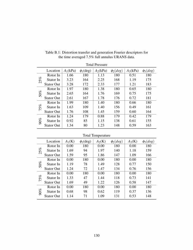
Table B.1: Distortion transfer and generation Fourier descriptors forthe time averaged 7.5% full annulus URANS data.

Total Pressure

Location A1(kPa) φ1(deg) A2(kPa) φ2(deg) A3(kPa) φ3(deg)

25%

Rotor In 1.66 180 1.13 180 0.51 180Stator In 3.23 164 2.25 168 1.19 175

Stator Out 3.28 172 2.33 177 1.21 183

50%


Stator Out 2.61 167 1.78 176 0.72 181

75%


Stator Out 1.76 108 1.45 159 0.60 164

90%


Stator Out 1.34 80 1.23 148 0.59 163

Total Temperature

Location A1(K) φ1(deg) A2(K) φ2(deg) A3(K) φ3(deg)

25%


Stator Out 1.59 95 1.86 147 1.09 166

50%


Stator Out 1.24 72 1.47 134 0.76 156

75%


Stator Out 1.69 49 1.22 126 0.58 147

90%


Stator Out 1.14 71 1.09 131 0.53 148

130

Table B.2: Distortion transfer and generation Fourier descriptors forthe radial and time averaged 7.5% full annulus URANS data.

Total Pressure

Location A1(kPa) φ1(deg) A2(kPa) φ2(deg) A3(kPa) φ3(deg)Rotor In 1.47 180 1.00 180 0.47 180Stator In 2.17 147 1.78 163 0.84 171

Stator Out 2.10 154 1.72 171 0.78 179

Total Temperature

Location A1(K) φ1(deg) A2(K) φ2(deg) A3(K) φ3(deg)Rotor In 0.00 180 0.00 180 0.00 180Stator In 1.44 82 1.46 136 0.77 155

Stator Out 1.38 86 1.39 142 0.70 162

131

Table B.3: Distortion transfer and generation Fourier descriptors forthe time averaged 15% full annulus URANS data.

Total Pressure

Location A1(kPa) φ1(deg) A2(kPa) φ2(deg) A3(kPa) φ3(deg)

25%


Stator Out 6.88 169 5.28 177 2.52 184

50%


Stator Out 6.15 163 4.61 178 1.78 183

75%


Stator Out 3.92 110 2.75 151 1.64 159

90%


Stator Out 3.40 78 2.91 140 1.83 158

Total Temperature

Location A1(K) φ1(deg) A2(K) φ2(deg) A3(K) φ3(deg)

25%


Stator Out 4.18 93 4.68 150 2.83 168

50%


Stator Out 3.98 64 3.97 135 2.15 155

75%


Stator Out 4.12 44 3.21 127 1.43 151

90%


Stator Out 3.19 65 2.82 132 1.50 147

132

Table B.4: Distortion transfer and generation Fourier descriptors forthe radial and time averaged 15% full annulus URANS data.

Total Pressure

Location A1(kPa) φ1(deg) A2(kPa) φ2(deg) A3(kPa) φ3(deg)Rotor In 3.24 180 2.25 180 1.09 180Stator In 4.35 136 3.71 159 1.71 168

Stator Out 4.78 151 3.91 171 1.92 178

Total Temperature

Location A1(K) φ1(deg) A2(K) φ2(deg) A3(K) φ3(deg)Rotor In 0.00 180 0.00 180 0.00 180Stator In 3.77 73 3.72 136 1.96 154

Stator Out 3.64 81 3.57 143 1.86 162

133

implementations of fourier methods in cfd to analyze

Documents