implementing an accelerated stability assessment program...
TRANSCRIPT
Implementing an Accelerated Stability
Assessment Program: Case Study
Cherokee Hoaglund Hyzer
With Special Thanks to Jeff Hofer, Timothy Kramer, Chad Wolfe, Seungyil
Yoon, Steve Baertschi and Ken Waterman
December 5, 2012
IVT’s Third Annual Forum on Stability Programs
2
Agenda
Accelerated Stability Assessment Program (ASAP)
•Overview and Background
•Study design
•Integrating ASAP with package modeling to predict product stability
Implementation - How Lilly is Currently Implementing the Program
•Accelerated stability template tools
•General process flow
•Considerations when performing an ASAP study
•Case Studies
Continuous Improvement - How Lilly is Improving the Program
•ASAP working group
•Process improvements
•ASAPprime™ software

3
• Arrhenius stability modeling has been used
successfully within the industry
• Lilly has not fully leveraged these stability tools and
approaches
• Pfizer has demonstrated a rapid, lean, and highly efficient approach to chemical stability screening that
involves non-traditional times/storage conditions and
statistical design and analysis of those experiments
• A business process and associated tools have been
developed to leverage this approach
Background
4
Accelerated Stability Assessment
Program (ASAP) Overview
• Modeling tool used in development that improves
product degradation understanding
• Has been shown in the literature to provide
credible predictions for shelf life/product expiry
estimations
• Faster than conventional stability and package
screening studies
• Scope
• Small molecule solid drug products, APIs,
excipients
Why Accelerated Stability?: Potential
Benefits
• Increased Scientific understanding of degradation mechanisms
• Specification rationale for purity
• Increased clinical start times
• Reduction of ICH stability re-dos
• Reduction of package screening studies prior to registration stability
• Flexibility for post-approval changes to stability commitments
• Can be used specifically in early in development to • compare prototype formulations
• identify stability issues (i.e. utilized as part of Genotoxic Impurities (GTI) control
strategy process in development)
• support risk assessment decisions for excipients
• identify proposed storage conditions
• identify acceptable CT packaging
5
6
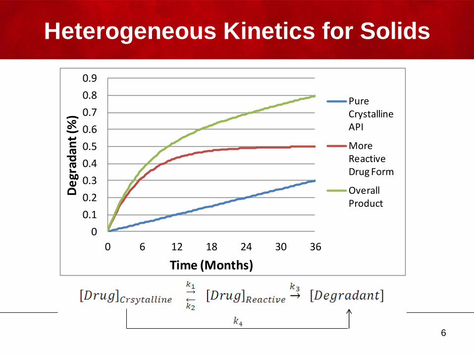
Heterogeneous Kinetics for Solids
0
0.1
0.2
0.3
0.4
0.5
0.6
0.7
0.8
0.9
0 6 12 18 24 30 36
De
grad
ant
(%)
Time (Months)
Pure Crystalline API
More Reactive Drug Form
Overall Product
7
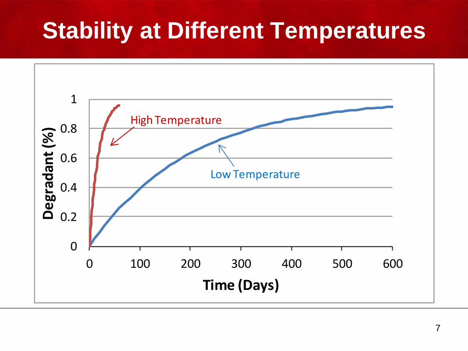
Stability at Different Temperatures
0
0.2
0.4
0.6
0.8
1
0 100 200 300 400 500 600
De
grad
ant
(%)
Time (Days)
Low Temperature
High Temperature
8
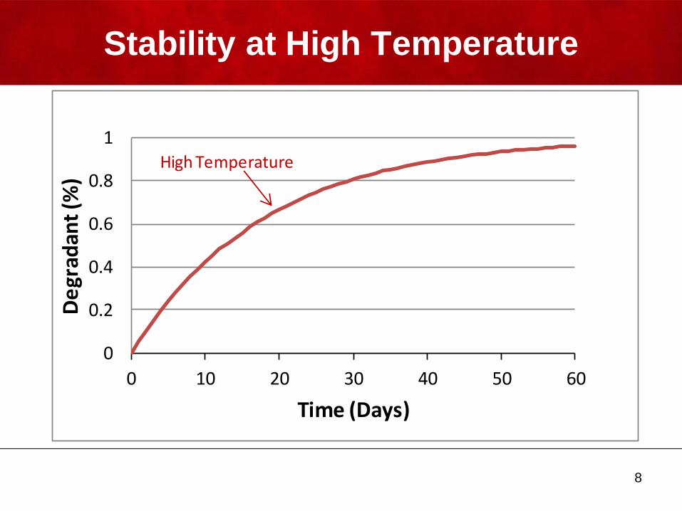
Stability at High Temperature
0
0.2
0.4
0.6
0.8
1
0 10 20 30 40 50 60
De
grad
ant
(%)
Time (Days)
High Temperature
9
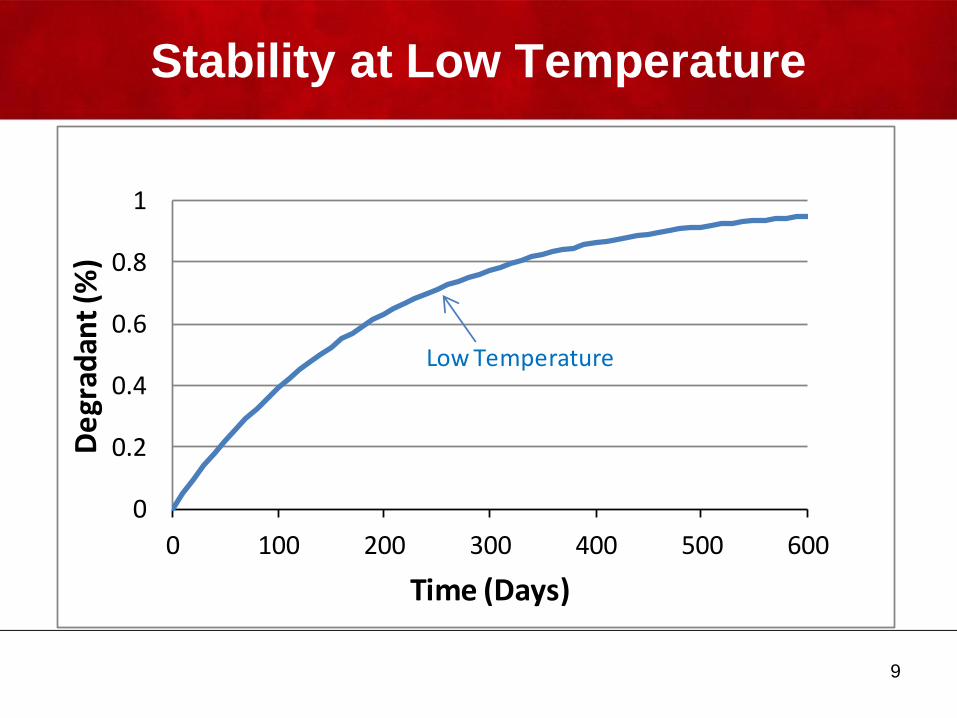
Stability at Low Temperature
0
0.2
0.4
0.6
0.8
1
0 100 200 300 400 500 600
De
grad
ant
(%)
Time (Days)
Low Temperature
10
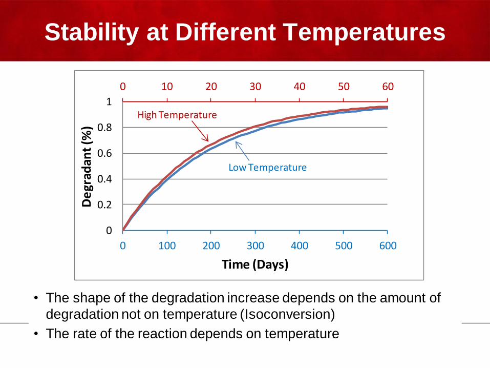
Stability at Different Temperatures
• The shape of the degradation increase depends on the amount of
degradation not on temperature (Isoconversion)
• The rate of the reaction depends on temperature
0 10 20 30 40 50 60
0
0.2
0.4
0.6
0.8
1
0 100 200 300 400 500 600
De
grad
ant
(%)
Time (Days)
Low Temperature
High Temperature
11
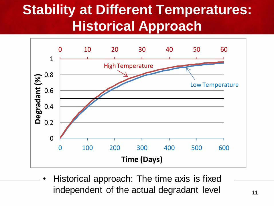
Stability at Different Temperatures:
Historical Approach
• Historical approach: The time axis is fixed
independent of the actual degradant level
0 10 20 30 40 50 60
0
0.2
0.4
0.6
0.8
1
0 100 200 300 400 500 600
De
grad
ant
(%)
Time (Days)
Low Temperature
High Temperature
12
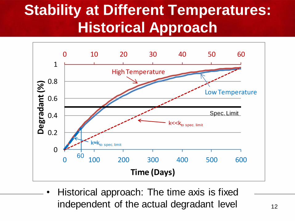
Stability at Different Temperatures:
Historical Approach
• Historical approach: The time axis is fixed
independent of the actual degradant level
0 10 20 30 40 50 60
0
0.2
0.4
0.6
0.8
1
0 100 200 300 400 500 600
De
grad
ant
(%)
Time (Days)
Low Temperature
High Temperature
60
k≈kto spec. limit
k<<kto spec. limit
Spec. Limit
13
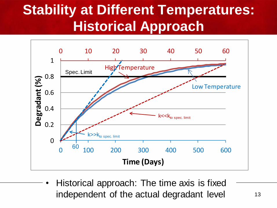
Stability at Different Temperatures:
Historical Approach
• Historical approach: The time axis is fixed
independent of the actual degradant level
0 10 20 30 40 50 60
0
0.2
0.4
0.6
0.8
1
0 100 200 300 400 500 600
De
grad
ant
(%)
Time (Days)
Low Temperature
High Temperature
60
k>>kto spec. limit
k<<kto spec. limit
Spec. Limit
14
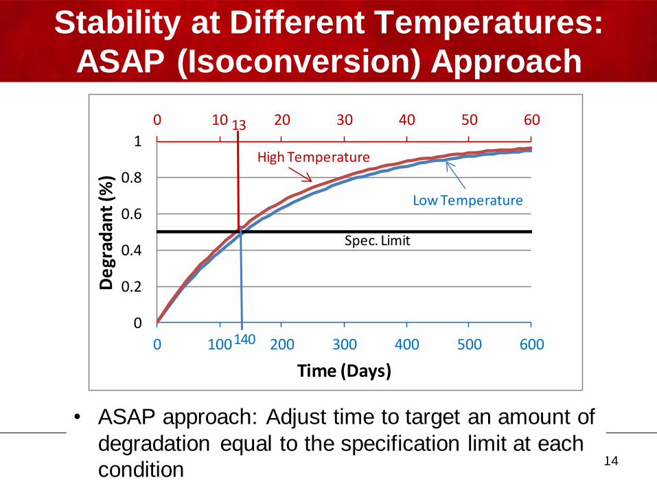
Stability at Different Temperatures:
ASAP (Isoconversion) Approach
• ASAP approach: Adjust time to target an amount of
degradation equal to the specification limit at each
condition
0 10 20 30 40 50 60
0
0.2
0.4
0.6
0.8
1
0 100 200 300 400 500 600
De
grad
ant
(%)
Time (Days)
Low Temperature
High Temperature
140
Spec. Limit
13
15
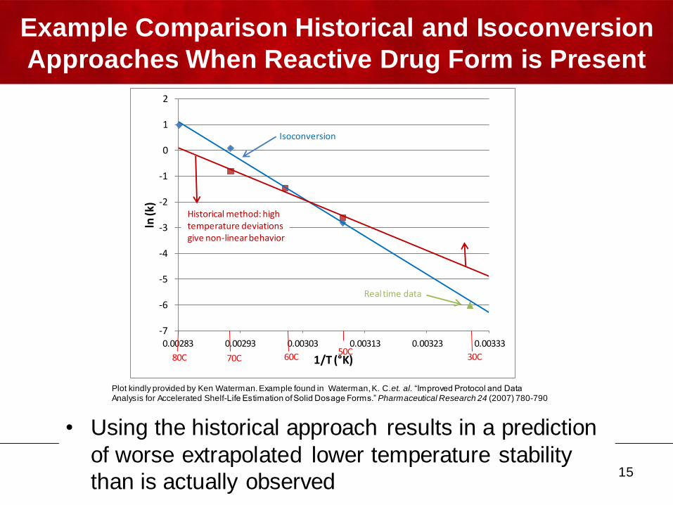
Example Comparison Historical and Isoconversion
Approaches When Reactive Drug Form is Present
• Using the historical approach results in a prediction
of worse extrapolated lower temperature stability
than is actually observed
-7
-6
-5
-4
-3
-2
-1
0
1
2
0.00283 0.00293 0.00303 0.00313 0.00323 0.00333
ln (k
)
1/T (°K)80C 70C 60C50C
30C
Isoconversion
Historical method: hightemperature deviationsgive non-linear behavior
Real time data
Plot kindly provided by Ken Waterman. Example found in Waterman, K. C.et. al. “Improved Protocol and Data Analysis for Accelerated Shelf-Life Estimation of Solid Dosage Forms.” Pharmaceutical Research 24 (2007) 780-790
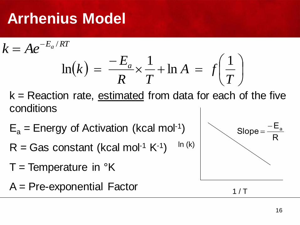
Arrhenius Model
TfA
TR
Ek a 1
ln1
ln
k = Reaction rate, estimated from data for each of the five conditions
Ea = Energy of Activation (kcal mol-1)
R = Gas constant (kcal mol-1 K-1)
T = Temperature in °K
A = Pre-exponential Factor
ln (k)
1 / T
R
ESlope a
16
RTEaAek/

Humidity Corrected Arrhenius Equation
)(ln1
ln ERHBATR
Ek a
humidity sensitivity factor
equilibrium relative humidity1/(isoconversion time)
17
Relative humidity in testing should be less
than the critical relative humidity (CRH)
Above CRH, sample dissolves, changing
phases – not representative of lower RHs.
(CRH is the humidity above which samples
deliquesce)
ln (k)
1 / T
collision frequency
activation energy
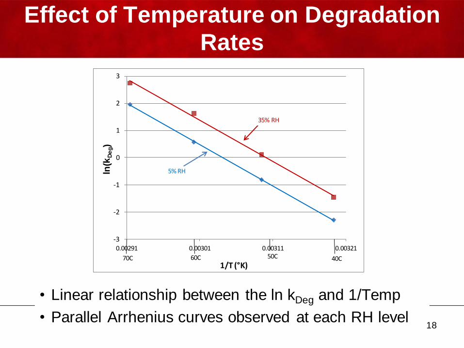
Effect of Temperature on Degradation
Rates
• Linear relationship between the ln kDeg and 1/Temp
• Parallel Arrhenius curves observed at each RH level 18
-3
-2
-1
0
1
2
3
0.00291 0.00301 0.00311 0.00321
ln (k
TRS)
1/T (°K)70C 60C 50C 40C
5% RH
35% RH
ln(k
De
g)
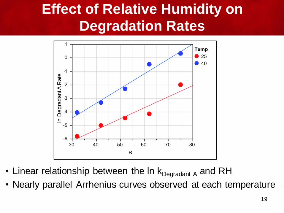
Effect of Relative Humidity on
Degradation Rates
• Linear relationship between the ln kDegradant A and RH
• Nearly parallel Arrhenius curves observed at each temperature
19
lnD
eg
rad
ant A
Rate
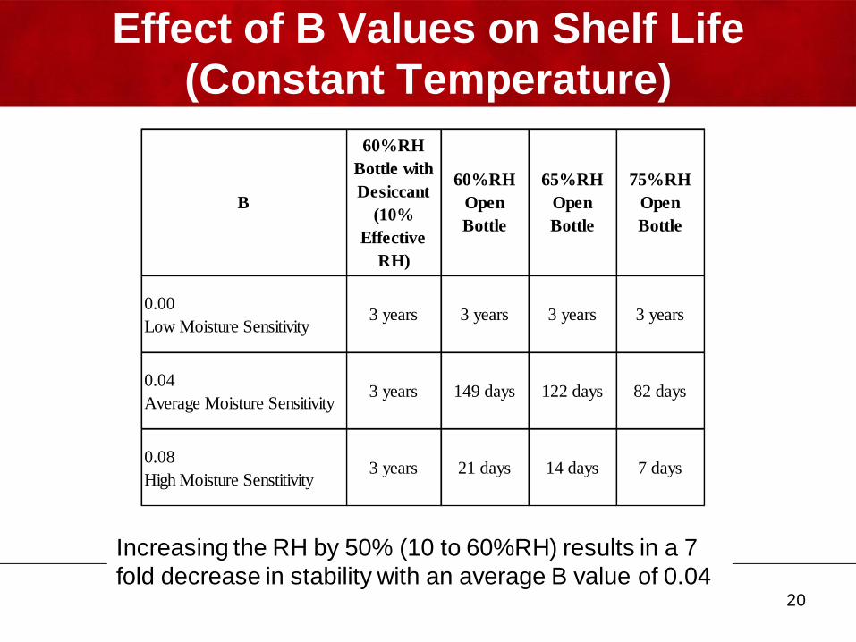
Effect of B Values on Shelf Life
(Constant Temperature)
20
Increasing the RH by 50% (10 to 60%RH) results in a 7
fold decrease in stability with an average B value of 0.04
B
60%RH
Bottle with
Desiccant
(10%
Effective
RH)
60%RH
Open
Bottle
65%RH
Open
Bottle
75%RH
Open
Bottle
0.00
Low Moisture Sensitivity3 years 3 years 3 years 3 years
0.04
Average Moisture Sensitivity3 years 149 days 122 days 82 days
0.08
High Moisture Senstitivity3 years 21 days 14 days 7 days
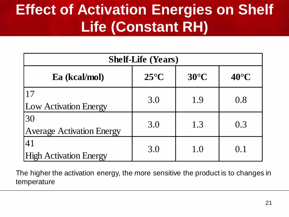
Effect of Activation Energies on Shelf
Life (Constant RH)
21
The higher the activation energy, the more sensitive the product is to changes in
temperature
Ea (kcal/mol) 25°C 30°C 40°C
17
Low Activation Energy3.0 1.9 0.8
30
Average Activation Energy3.0 1.3 0.3
41
High Activation Energy3.0 1.0 0.1
Shelf-Life (Years)
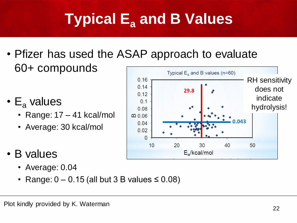
Typical Ea and B Values
22
RH sensitivity
does not
indicate
hydrolysis!
Plot kindly provided by K. Waterman
• Pfizer has used the ASAP approach to evaluate
60+ compounds
• Ea values• Range: 17 – 41 kcal/mol
• Average: 30 kcal/mol
• B values• Average: 0.04
• Range: 0 – 0.15 (all but 3 B values ≤ 0.08)
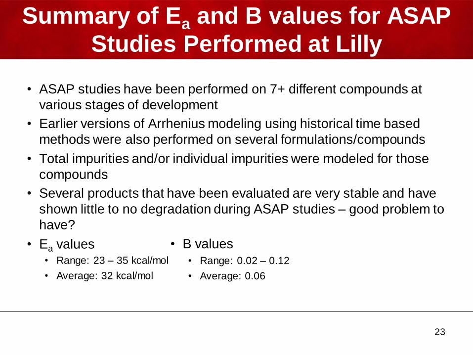
Summary of Ea and B values for ASAP
Studies Performed at Lilly
• ASAP studies have been performed on 7+ different compounds at
various stages of development
• Earlier versions of Arrhenius modeling using historical time based
methods were also performed on several formulations/compounds
• Total impurities and/or individual impurities were modeled for those
compounds
• Several products that have been evaluated are very stable and have
shown little to no degradation during ASAP studies – good problem to
have?
• Ea values• Range: 23 – 35 kcal/mol
• Average: 32 kcal/mol
23
• B values
• Range: 0.02 – 0.12
• Average: 0.06
0.00
0.02
0.04
0.06
0.08
0.10
0.12
0.14
20 25 30 35 40
B V
alu
e
Ea kcal/mol
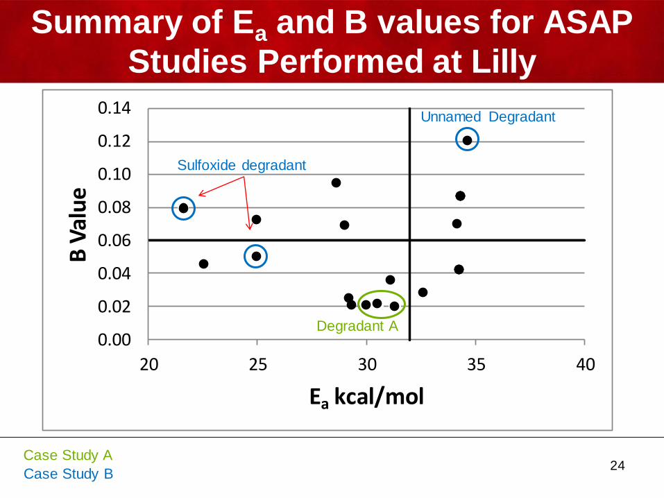
Summary of Ea and B values for ASAP
Studies Performed at Lilly
24
Sulfoxide degradant
Degradant A
Case Study B
Case Study A
0.00
0.02
0.04
0.06
0.08
0.10
0.12
0.14
20 25 30 35 40
B V
alu
e
Ea kcal/mol0.00
0.02
0.04
0.06
0.08
0.10
0.12
0.14
20 25 30 35 40
B V
alu
e
Ea kcal/mol0.00
0.02
0.04
0.06
0.08
0.10
0.12
0.14
20 25 30 35 40
B V
alu
e
Ea kcal/mol
0.00
0.02
0.04
0.06
0.08
0.10
0.12
0.14
20 25 30 35 40
B V
alu
e
Ea kcal/mol
0.00
0.02
0.04
0.06
0.08
0.10
0.12
0.14
20 25 30 35 40
B V
alu
e
Ea kcal/mol
Unnamed Degradant
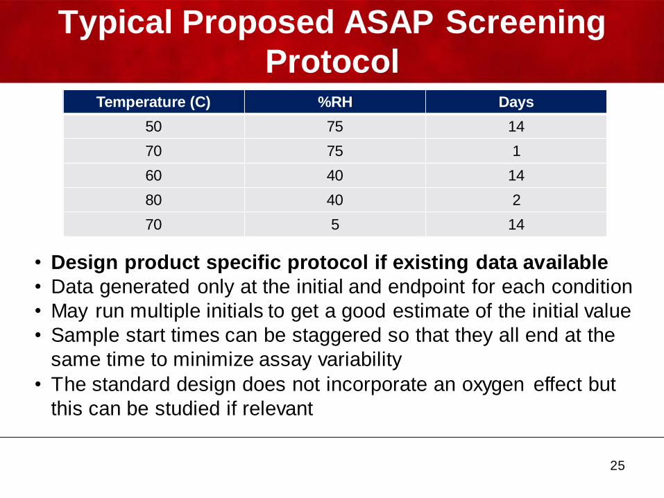
Typical Proposed ASAP Screening
Protocol
25
• Design product specific protocol if existing data available
• Data generated only at the initial and endpoint for each condition
• May run multiple initials to get a good estimate of the initial value
• Sample start times can be staggered so that they all end at the
same time to minimize assay variability
• The standard design does not incorporate an oxygen effect but
this can be studied if relevant
Temperature (C) %RH Days
50 75 14
70 75 1
60 40 14
80 40 2
70 5 14
Study Analysis
• Rate of change data modeled to provide estimates of
temperature and RH effects
• Estimates can be used to compare formulations and support
risk assessment decisions for excipients including supporting
excipient selection or continued excipient use
• External humidity protection provided by packaging
• Change in RH over time for package is combined with
degradation estimates to generate predicted degradation
profiles for each package and storage condition
combination and support initial container closure selection
strategy
26
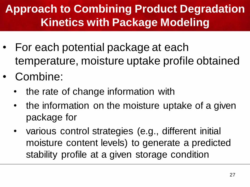
Approach to Combining Product Degradation
Kinetics with Package Modeling
• For each potential package at each
temperature, moisture uptake profile obtained
• Combine:
• the rate of change information with
• the information on the moisture uptake of a given
package for
• various control strategies (e.g., different initial
moisture content levels) to generate a predicted
stability profile at a given storage condition
27
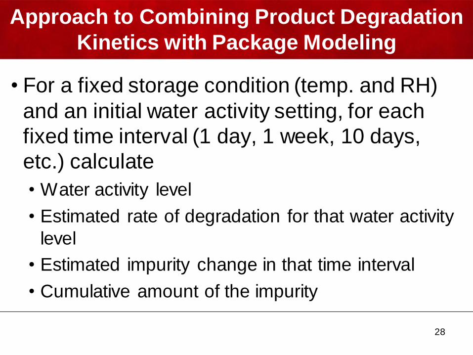
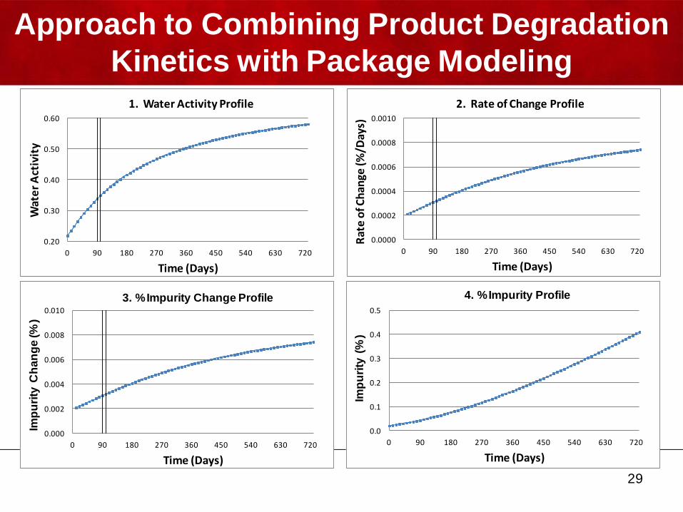
• For a fixed storage condition (temp. and RH)
and an initial water activity setting, for each
fixed time interval (1 day, 1 week, 10 days,
etc.) calculate
• Water activity level
• Estimated rate of degradation for that water activity
level
• Estimated impurity change in that time interval
• Cumulative amount of the impurity
28
Approach to Combining Product Degradation
Kinetics with Package Modeling
29
Approach to Combining Product Degradation
Kinetics with Package Modeling
0.20
0.30
0.40
0.50
0.60
0 90 180 270 360 450 540 630 720
Wat
er
Act
ivit
y
Time (Days)
1. Water Activity Profile
0.0000
0.0002
0.0004
0.0006
0.0008
0.0010
0 90 180 270 360 450 540 630 720
Rat
e o
f Ch
ange
(%/D
ays)
Time (Days)
2. Rate of Change Profile
0.0
0.1
0.2
0.3
0.4
0.5
0 90 180 270 360 450 540 630 720
TDP
(%)
Time (Days)
4. TDP Profile4. %Impurity Profile
Imp
uri
ty (
%)
0.000
0.002
0.004
0.006
0.008
0.010
0 90 180 270 360 450 540 630 720
TDP
Ch
ange
(%
)
Time (Days)
3. TDP Change Profile3. %Impurity Change Profile
Imp
uri
ty C
ha
ng
e (%
)
30
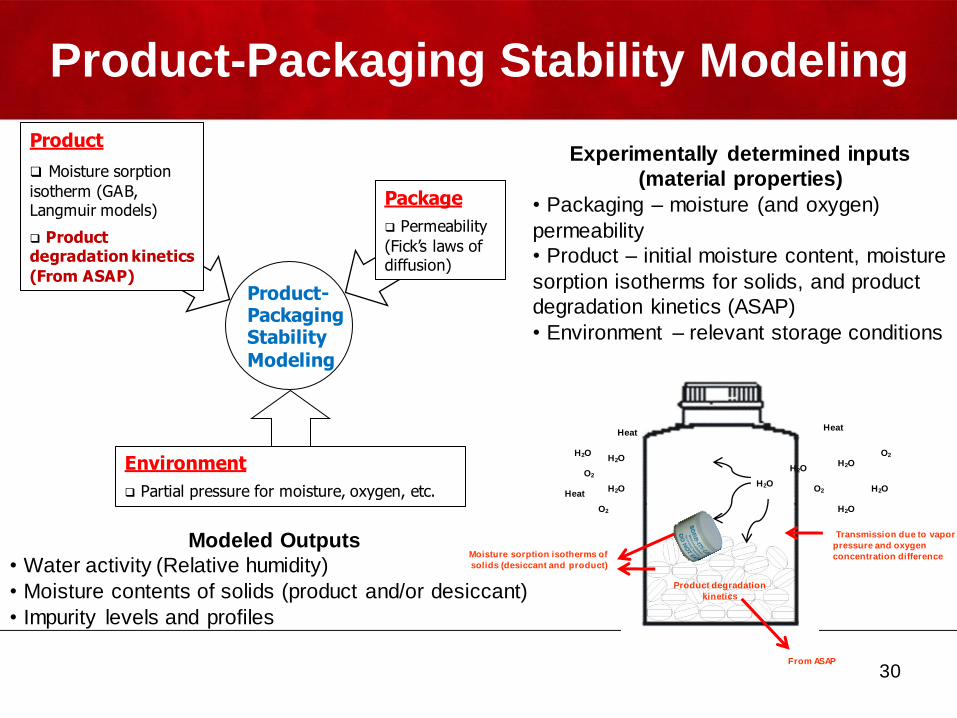
Environment
Partial pressure for moisture, oxygen, etc.
Product-Packaging Stability Modeling
Package
Permeability
(Fick’s laws of diffusion)
Product
Moisture sorption
isotherm (GAB, Langmuir models)
Product degradation kinetics
(From ASAP)
H2OH2O
H2O
H2OH2O
H2O
H2O
Transmission due to vapor
pressure and oxygen
concentration differenceMoisture sorption isotherms of
solids (desiccant and product)
O2
O2
O2
O2
Product degradation
kinetics
HeatHeat
HeatH2O
From ASAP
Experimentally determined inputs
(material properties)
• Packaging – moisture (and oxygen)
permeability
• Product – initial moisture content, moisture
sorption isotherms for solids, and product
degradation kinetics (ASAP)
• Environment – relevant storage conditions
Modeled Outputs
• Water activity (Relative humidity)
• Moisture contents of solids (product and/or desiccant)
• Impurity levels and profiles
Product-Packaging Stability Modeling
How Lilly Implemented the Program…
• Small group of scientists and statisticians assembled
to assess ASAP and develop a pilot
process/implementation plan
• Information repository developed that included
literature articles (or references) and presentations to
help educate scientists/statisticians
• A defined process and Excel based tools were
developed to facilitate implementation
• Integration with existing package modeling tools
31
Accelerated Stability Template Tool
32
• Non-validated Excel Spreadsheet
• Assumes that only an initial and final time point
are collected for each storage condition
• Calculates the coefficients for the parameters
(intercept, temperature, and RH) which serve as
inputs into the packaging tool to determine the
feasibility of packages
• Calculates a coefficient for oxygen if studied
• Uses named ranges, allowing the coefficient
estimates to be compiled into a database
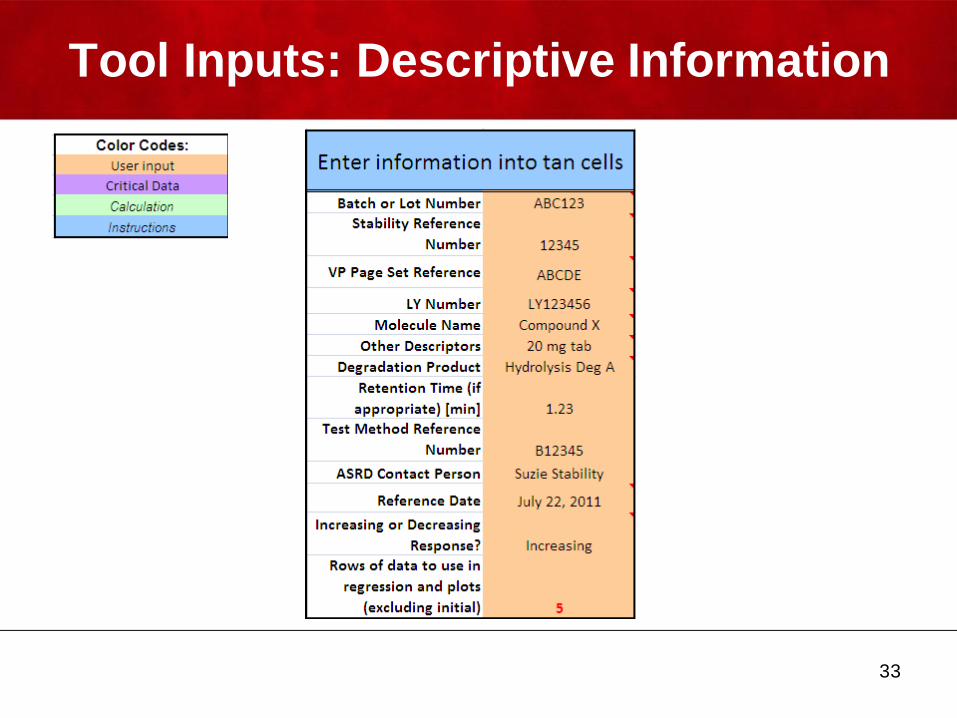
Tool Inputs: Descriptive Information
33
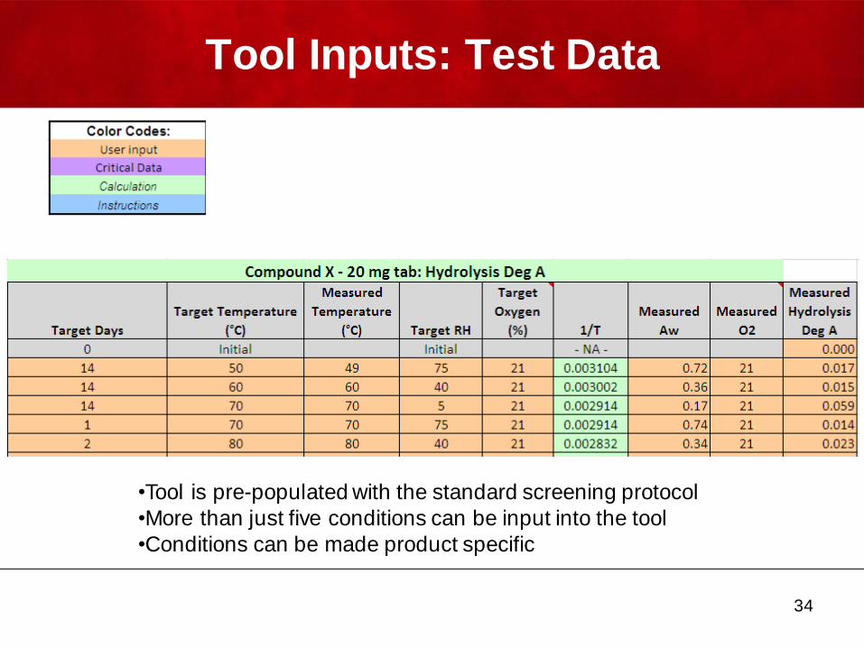
Tool Inputs: Test Data
•Tool is pre-populated with the standard screening protocol
•More than just five conditions can be input into the tool
•Conditions can be made product specific
34
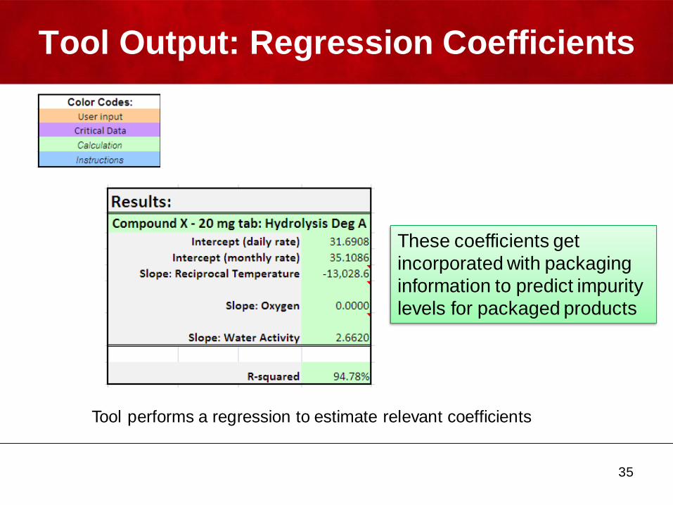
Tool Output: Regression Coefficients
These coefficients get
incorporated with packaging
information to predict impurity
levels for packaged products
Tool performs a regression to estimate relevant coefficients
35
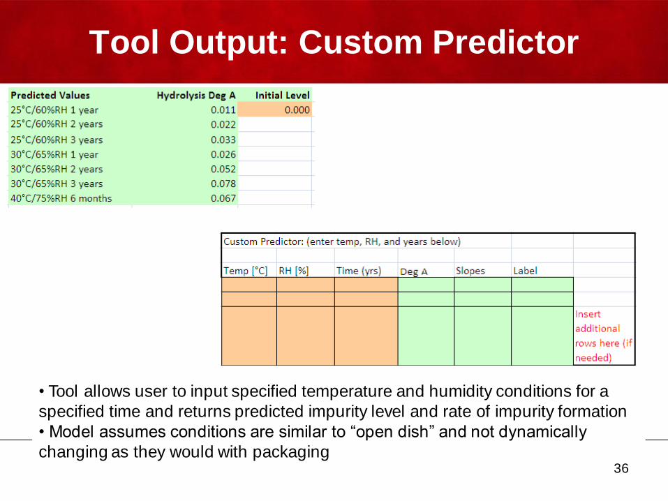
Tool Output: Custom Predictor
• Tool allows user to input specified temperature and humidity conditions for a
specified time and returns predicted impurity level and rate of impurity formation
• Model assumes conditions are similar to “open dish” and not dynamically
changing as they would with packaging36
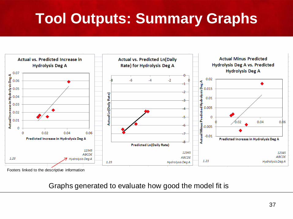
Tool Outputs: Summary Graphs
Graphs generated to evaluate how good the model fit is
Footers linked to the descriptive information
37
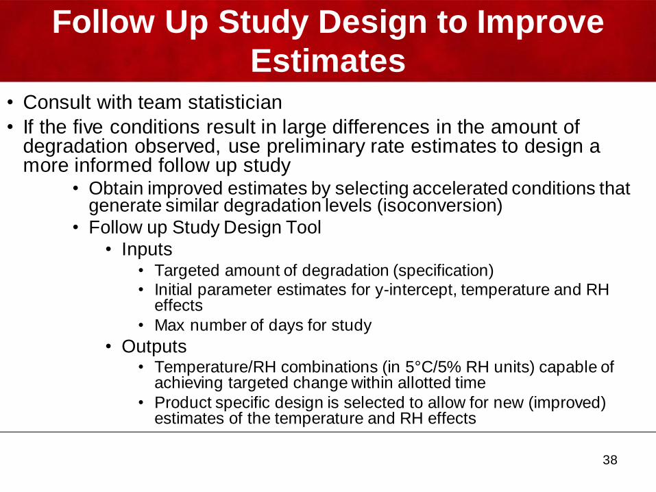
Follow Up Study Design to Improve
Estimates• Consult with team statistician
• If the five conditions result in large differences in the amount of degradation observed, use preliminary rate estimates to design a more informed follow up study
• Obtain improved estimates by selecting accelerated conditions that generate similar degradation levels (isoconversion)
• Follow up Study Design Tool
• Inputs• Targeted amount of degradation (specification)• Initial parameter estimates for y-intercept, temperature and RH
effects
• Max number of days for study
• Outputs• Temperature/RH combinations (in 5°C/5% RH units) capable of
achieving targeted change within allotted time
• Product specific design is selected to allow for new (improved) estimates of the temperature and RH effects
38
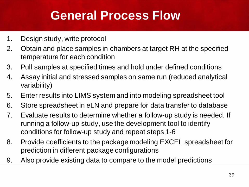
General Process Flow
1. Design study, write protocol
2. Obtain and place samples in chambers at target RH at the specified
temperature for each condition
3. Pull samples at specified times and hold under defined conditions
4. Assay initial and stressed samples on same run (reduced analytical
variability)
5. Enter results into LIMS system and into modeling spreadsheet tool
6. Store spreadsheet in eLN and prepare for data transfer to database
7. Evaluate results to determine whether a follow-up study is needed. If
running a follow-up study, use the development tool to identify
conditions for follow-up study and repeat steps 1-6
8. Provide coefficients to the package modeling EXCEL spreadsheet for
prediction in different package configurations
9. Also provide existing data to compare to the model predictions
39
Considerations When Performing an
ASAP Study
• Stability predictions are most accurate for the isoconversion point
which is generally chosen as the degradant’s specified or
anticipated limit (specification)
• Coefficient estimates are specific to the impurity that was modeled
and the formulation that was used
• Coefficient estimates need to be calculated for each impurity of interest
• If the formulation changes, the study must be repeated with the new formulation to estimate formulation specific coefficients
• Consider potential failure modes (e.g. Form/Phase change caused
by melts, glass transitions, anhydrate/hydrate formation)
• ASAP paradigm focuses on chemical degradation and is not
intended for physical changes such as dissolution due to the
potential non-Arrhenius behaviors of these properties
40
Impact on Control Strategy and Design
Space
Predictive models can be used to address different
manufacturing control strategies and package
configuration combinations
• What if initial water activity was lower or higher?
• Would more protective packaging allow a higher initial
water activity?
• If yes, is it worth the additional cost?
• Would less protective packaging be possible if the
starting water activity were lower?
• How big of an impact is this?
41
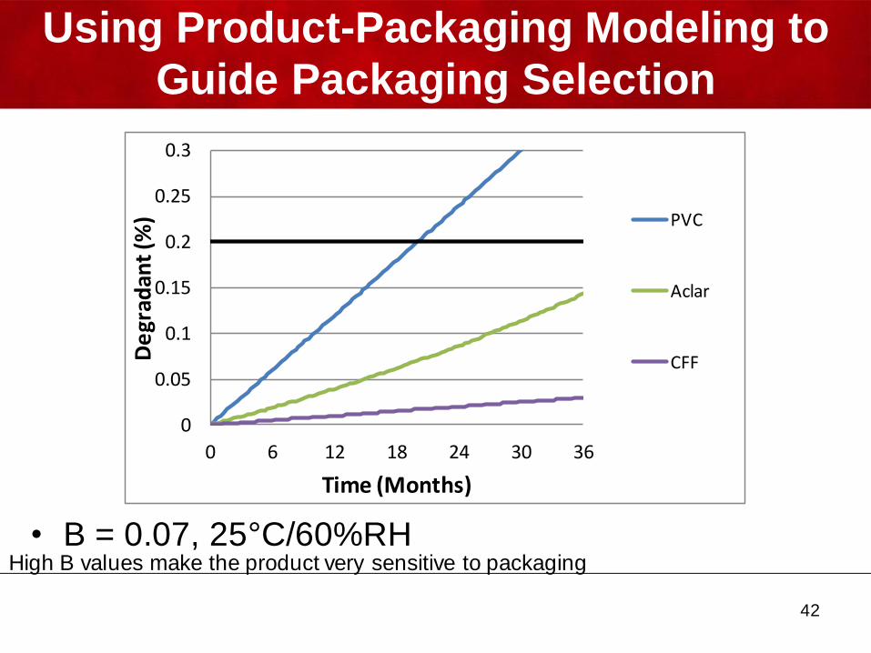
Using Product-Packaging Modeling to
Guide Packaging Selection
• B = 0.07, 25°C/60%RH
42
High B values make the product very sensitive to packaging
0
0.05
0.1
0.15
0.2
0.25
0.3
0 6 12 18 24 30 36
De
grad
ant
(%)
Time (Months)
PVC
Aclar
CFF
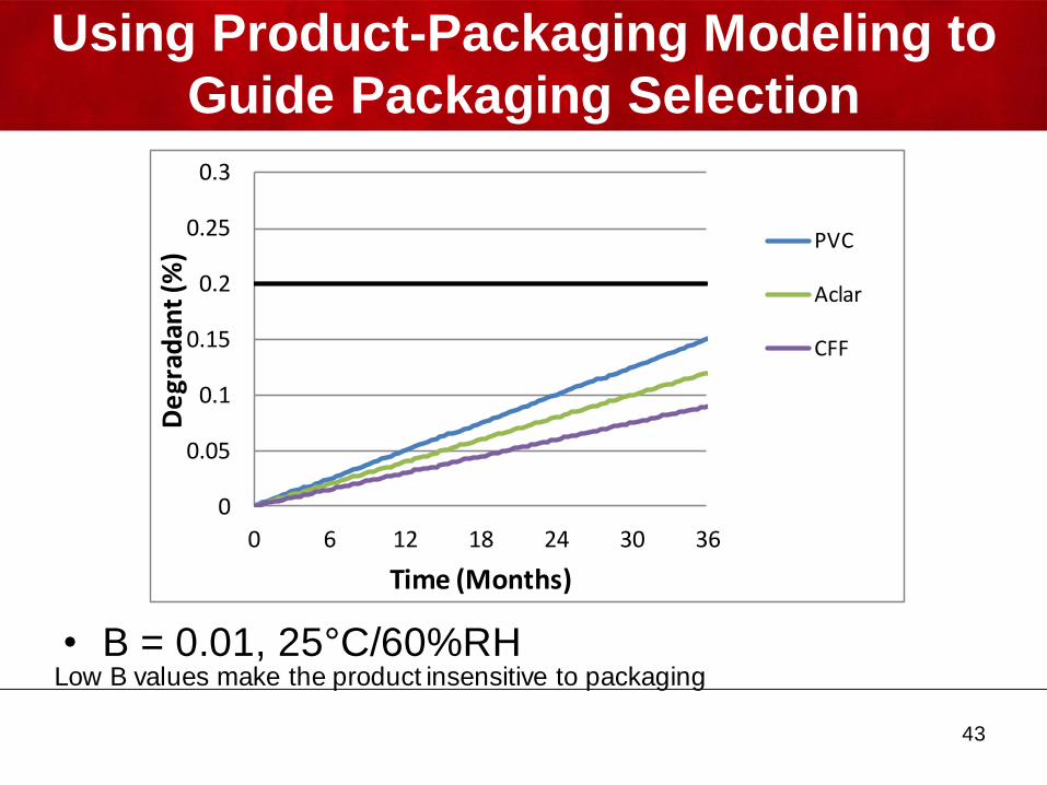
Using Product-Packaging Modeling to
Guide Packaging Selection
• B = 0.01, 25°C/60%RH
43
Low B values make the product insensitive to packaging
0
0.05
0.1
0.15
0.2
0.25
0.3
0 6 12 18 24 30 36
De
grad
ant
(%)
Time (Months)
PVC
Aclar
CFF
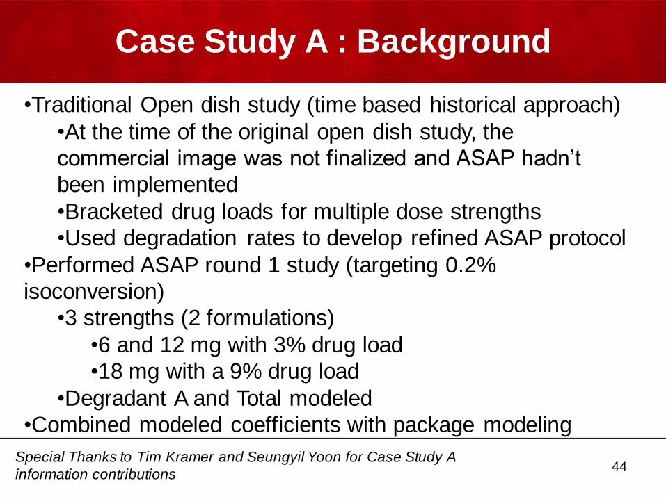
Case Study A : Background
•Traditional Open dish study (time based historical approach)
•At the time of the original open dish study, the
commercial image was not finalized and ASAP hadn’t
been implemented
•Bracketed drug loads for multiple dose strengths
•Used degradation rates to develop refined ASAP protocol
•Performed ASAP round 1 study (targeting 0.2%
isoconversion)
•3 strengths (2 formulations)
•6 and 12 mg with 3% drug load
•18 mg with a 9% drug load
•Degradant A and Total modeled
•Combined modeled coefficients with package modeling
44Special Thanks to Tim Kramer and Seungyil Yoon for Case Study A
information contributions
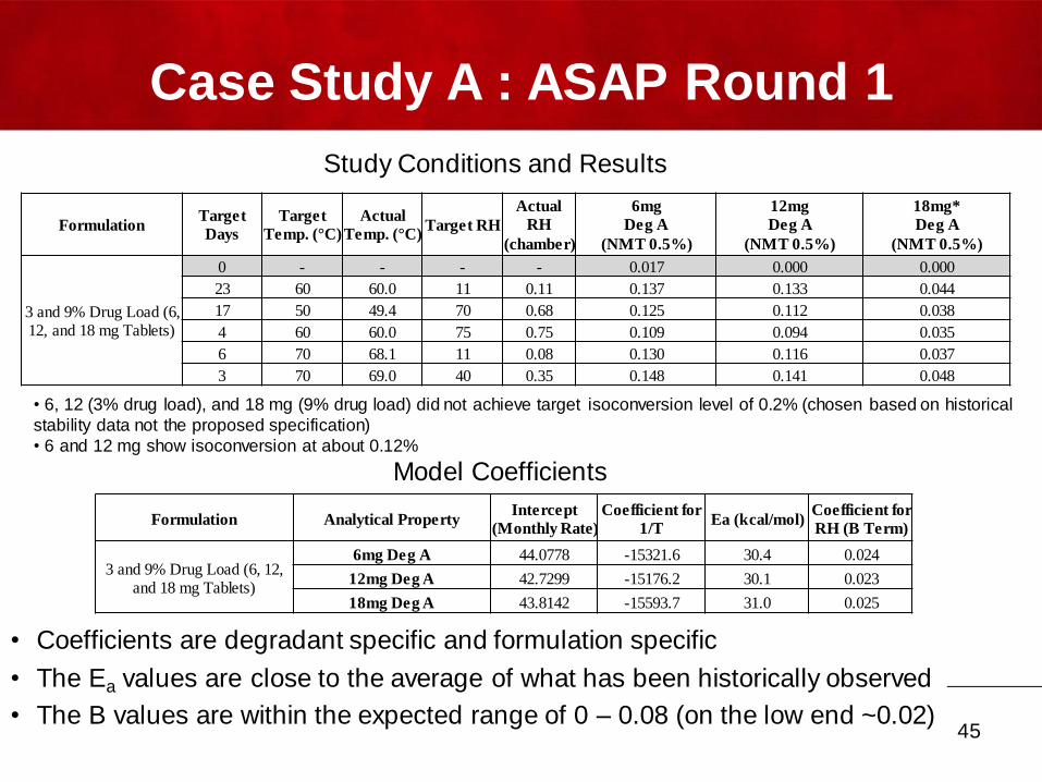
Case Study A : ASAP Round 1
Formulation Analytical PropertyIntercept
(Monthly Rate)
Coefficient for
1/TEa (kcal/mol)
Coefficient for
RH (B Term)
3 and 9% Drug Load (6, 12, and 18 mg Tablets)
6mg Deg A 44.0778 -15321.6 30.4 0.024
12mg Deg A 42.7299 -15176.2 30.1 0.023
18mg Deg A 43.8142 -15593.7 31.0 0.025
FormulationTarget
Days
Target
Temp. (°C)
Actual
Temp. (°C)Target RH
Actual
RH
(chamber)
6mg
Deg A
(NMT 0.5%)
12mg
Deg A
(NMT 0.5%)
18mg*
Deg A
(NMT 0.5%)
3 and 9% Drug Load (6, 12, and 18 mg Tablets)
0 - - - - 0.017 0.000 0.000
23 60 60.0 11 0.11 0.137 0.133 0.044
17 50 49.4 70 0.68 0.125 0.112 0.038
4 60 60.0 75 0.75 0.109 0.094 0.035
6 70 68.1 11 0.08 0.130 0.116 0.037
3 70 69.0 40 0.35 0.148 0.141 0.048
Study Conditions and Results
Model Coefficients
• 6, 12 (3% drug load), and 18 mg (9% drug load) did not achieve target isoconversion level of 0.2% (chosen based on historical
stability data not the proposed specification)
• 6 and 12 mg show isoconversion at about 0.12%
• Coefficients are degradant specific and formulation specific
• The Ea values are close to the average of what has been historically observed
• The B values are within the expected range of 0 – 0.08 (on the low end ~0.02)45
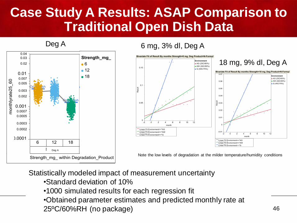
Case Study A Results: ASAP Comparison to Traditional Open Dish Data
Statistically modeled impact of measurement uncertainty
•Standard deviation of 10%
•1000 simulated results for each regression fit
•Obtained parameter estimates and predicted monthly rate at
25ºC/60%RH (no package)
Deg A
Deg A
6 mg, 3% dl, Deg A
18 mg, 9% dl, Deg A
46
Note the low levels of degradation at the milder temperature/humidity conditions
0
0.05
0.1
0.15
0.2
0.25
0.3
0 50 100 150 200
De
gra
da
nt A
(%
)
Time (days)
6 mg (3% dl)
Deg A at 40⁰C/75% RH
PVC
4 ct
2 mil Aclar
30 ct
1000 ct
Al foil
PVC_est
4 ct_est
2 mil Aclar_est
30 ct_est
1000 ct_est
Al foil_est
0
0.01
0.02
0.03
0.04
0.05
0.06
0.07
0 50 100 150 200
De
gra
da
nt A
(%
)
Time (days)
6 mg (3% dl)
Deg A at 25⁰C/60% RH
PVC
4 ct
2 mil Aclar
30 ct
1000 ct
PVC_est
4 ct_est
2 mil Aclar_est
30 ct_est
1000 ct_est
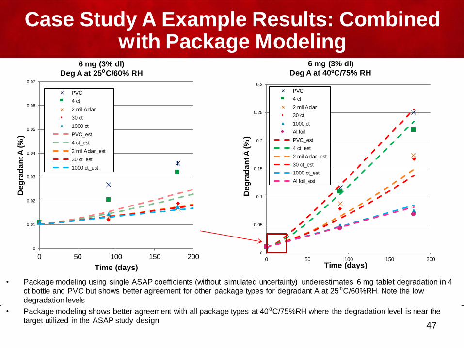
Case Study A Example Results: Combined with Package Modeling
• Package modeling using single ASAP coefficients (without simulated uncertainty) underestimates 6 mg tablet degradation in 4
ct bottle and PVC but shows better agreement for other package types for degradant A at 25⁰C/60%RH. Note the low
degradation levels
• Package modeling shows better agreement with all package types at 40⁰C/75%RH where the degradation level is near the
target utilized in the ASAP study design47
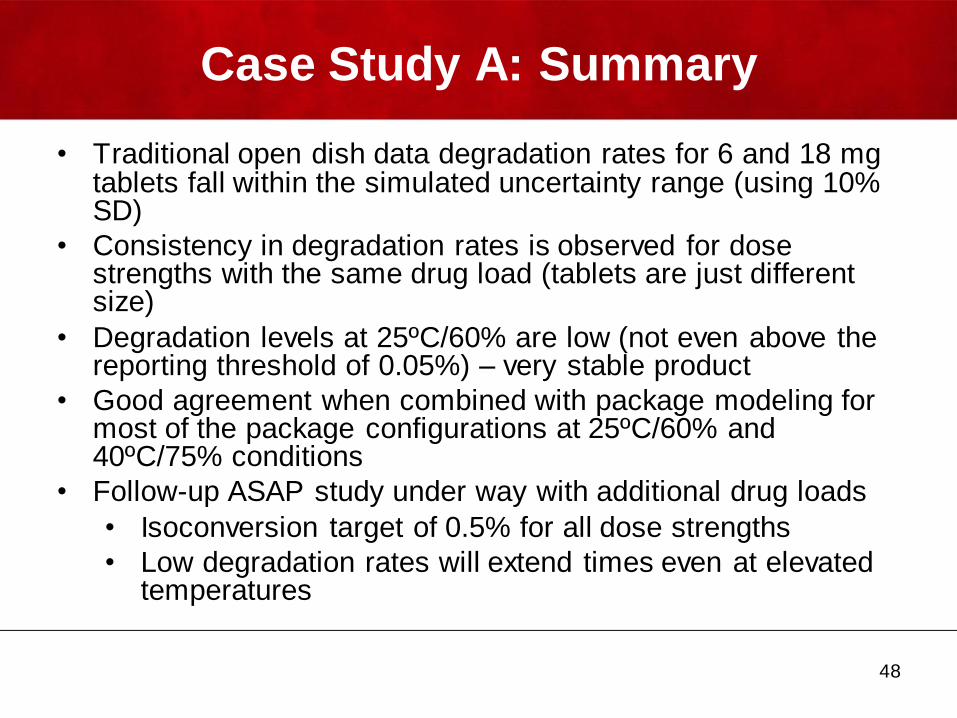
Case Study A: Summary
• Traditional open dish data degradation rates for 6 and 18 mg tablets fall within the simulated uncertainty range (using 10% SD)
• Consistency in degradation rates is observed for dose strengths with the same drug load (tablets are just different size)
• Degradation levels at 25ºC/60% are low (not even above the reporting threshold of 0.05%) – very stable product
• Good agreement when combined with package modeling for most of the package configurations at 25ºC/60% and 40ºC/75% conditions
• Follow-up ASAP study under way with additional drug loads
• Isoconversion target of 0.5% for all dose strengths
• Low degradation rates will extend times even at elevated temperatures
48
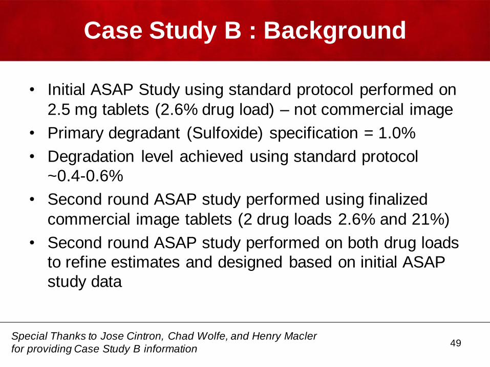
Case Study B : Background
49
• Initial ASAP Study using standard protocol performed on
2.5 mg tablets (2.6% drug load) – not commercial image
• Primary degradant (Sulfoxide) specification = 1.0%
• Degradation level achieved using standard protocol
~0.4-0.6%
• Second round ASAP study performed using finalized
commercial image tablets (2 drug loads 2.6% and 21%)
• Second round ASAP study performed on both drug loads
to refine estimates and designed based on initial ASAP
study data
Special Thanks to Jose Cintron, Chad Wolfe, and Henry Macler
for providing Case Study B information
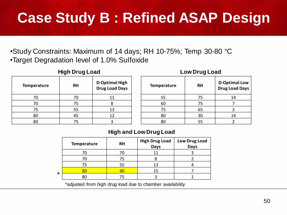
Temperature RHD-Optimal High Drug Load Days
70 70 11
70 75 8
75 55 13
80 45 12
80 75 3
Temperature RHD-Optimal Low Drug Load Days
55 75 14
60 75 7
75 65 2
80 30 14
80 55 2
Temperature RHHigh Drug Load
DaysLow Drug Load
Days
70 70 11 3
70 75 8 2
75 55 13 4
80 40 15 7
80 75 3 1
•Study Constraints: Maximum of 14 days; RH 10-75%; Temp 30-80 °C•Target Degradation level of 1.0% Sulfoxide
High Drug Load Low Drug Load
High and Low Drug Load
*
*adjusted from high drug load due to chamber availability
Case Study B : Refined ASAP Design
50
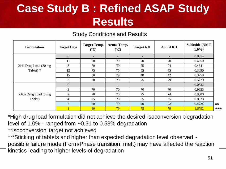
Formulation Target DaysTarget Temp.
(°C)
Actual Temp.
(°C)Target RH Actual RH
Sulfoxide (NMT
1.0%)
21% Drug Load (20 mg
Tablet) *
0 - - - - 0.0614
11 70 70 70 70 0.4650
8 70 70 75 74 0.4641
13 75 75 55 55 0.3090
15 80 79 40 42 0.3758
3 80 79 75 79 0.5279
2.6% Drug Load (5 mg
Tablet)
0 - - - - 0.0832
3 70 70 70 70 0.9855
2 70 70 75 74 0.9308
4 75 75 55 55 0.8573
7 80 79 40 42 0.4724
1 80 79 75 79 1.6792
*High drug load formulation did not achieve the desired isoconversion degradation
level of 1.0% - ranged from ~0.31 to 0.53% degradation
**Isoconversion target not achieved
***Sticking of tablets and higher than expected degradation level observed -
possible failure mode (Form/Phase transition, melt) may have affected the reaction kinetics leading to higher levels of degradation
**
51
***
Case Study B : Refined ASAP Study
ResultsStudy Conditions and Results
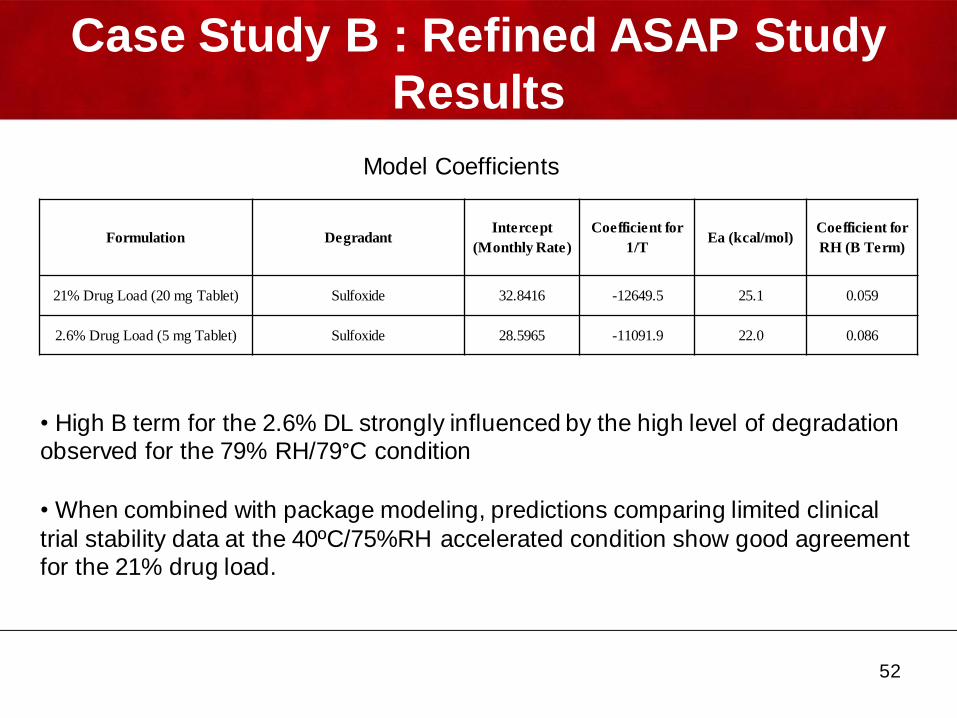
Formulation DegradantIntercept
(Monthly Rate)
Coefficient for
1/TEa (kcal/mol)
Coefficient for
RH (B Term)
21% Drug Load (20 mg Tablet) Sulfoxide 32.8416 -12649.5 25.1 0.059
2.6% Drug Load (5 mg Tablet) Sulfoxide 28.5965 -11091.9 22.0 0.086
• High B term for the 2.6% DL strongly influenced by the high level of degradation observed for the 79% RH/79°C condition
• When combined with package modeling, predictions comparing limited clinical
trial stability data at the 40ºC/75%RH accelerated condition show good agreement for the 21% drug load.
52
Case Study B : Refined ASAP Study
Results
Model Coefficients
0.0
0.1
0.2
0.3
0.4
0.5
0.6
0.7
0.8
0 50 100 150 200
Water Activity, 20 mg
ModeledCT
0.0
0.2
0.4
0.6
0.8
1.0
0 50 100 150 200
% Sulfoxide, 20 mg
Modeled
CT
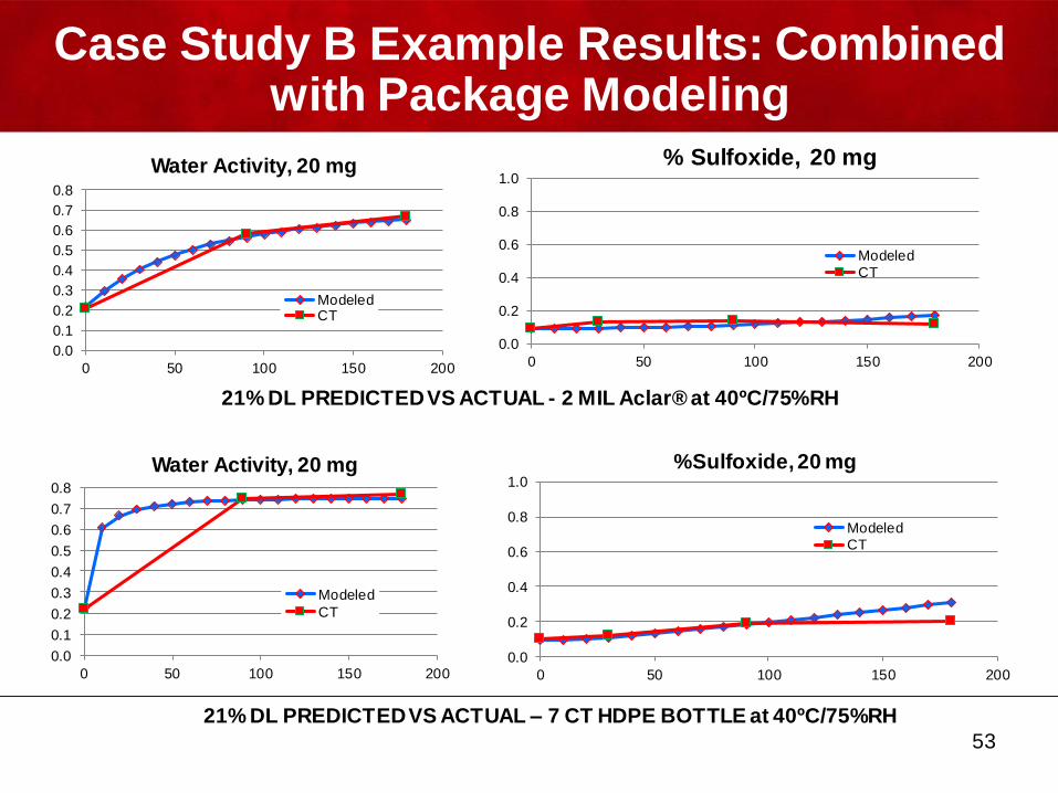
21% DL PREDICTED VS ACTUAL - 2 MIL Aclar® at 40ºC/75%RH
Case Study B Example Results: Combined with Package Modeling
0.0
0.1
0.2
0.3
0.4
0.5
0.6
0.7
0.8
0 50 100 150 200
Water Activity, 20 mg
Modeled
CT
0.0
0.2
0.4
0.6
0.8
1.0
0 50 100 150 200
%Sulfoxide, 20 mg
ModeledCT
21% DL PREDICTED VS ACTUAL – 7 CT HDPE BOTTLE at 40ºC/75%RH
53
Temp. (°C) RH Days
65 75 34
70 70 26
70 75 20
75 60 28
75 75 11
Temp. (°C) RH Days
50 75 14
65 75 3
70 55 10
75 50 10
75 65 3
Temp. (°C) RH Days
65 75 3
70 70 3
70 75 2
75 60 4
75 75 1
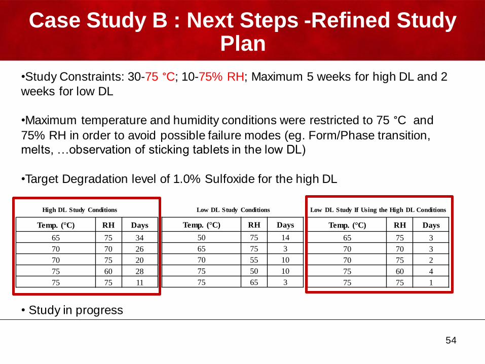
High DL Study Conditions Low DL Study Conditions Low DL Study If Using the High DL Conditions
•Study Constraints: 30-75 °C; 10-75% RH; Maximum 5 weeks for high DL and 2
weeks for low DL
•Maximum temperature and humidity conditions were restricted to 75 °C and
75% RH in order to avoid possible failure modes (eg. Form/Phase transition, melts, …observation of sticking tablets in the low DL)
•Target Degradation level of 1.0% Sulfoxide for the high DL
• Study in progress
Case Study B : Next Steps -Refined Study Plan
54
Continuous Improvement – How Lilly is
Improving the Program
• ASAP Working Group Construct
• Seek interest and build expertise across specialty areas
(cross-functional Subject Matter Experts)
• Analytical
• Stats
• Formulation
• Packaging
• Preformulation
• Assess implementation and impact of using ASAP to portfolio
• Share case studies and learning (results, predictions, etc.)
• Improving processes, tools (including software purchase), and study
execution
• Can help leverage getting needed resources for studies to intentionally
explore failure modes
55
Process Improvements
• Improve study execution concepts
• Focus on isoconversion and degradant(s) that drive the
degradation product control strategy
• Increased capacity
• Additional ovens/incubators
• Understanding Equilibration and Failure Mode Questions
• How do we know that coated tablets have equilibrated to
the incubator conditions? Pre-equilibration at ambient
temperature? Do we accept? Closed versus open
systems?
• Best practices to understand potential failure modes to
inform study design –what questions do we ask up front?
56
ASAPprimeTM Software
• Commercially available validated statistical modeling
software based on the ASAP paradigm
• Developed by Ken Waterman who pioneered this
approach at Pfizer and founded FreeThink Technologies
Inc.
• Analyzes the effects of temperature and relative humidity
on product stability
• Performs Monte-Carlo simulations to estimate confidence
intervals for a projected shelf-life under various storage
conditions
• The software nicely integrates product and packaging
modeling components
57http://freethinktech.com/
Summary
• Historical approach• Fixed time points for all accelerated conditions that are not necessarily designed to
give equal amounts of degradation (isoconversion)
• Extrapolation to real time conditions is often limited
• Package selection requires package screening studies with at least 6 months of
stability data
• ASAP approach• Scientifically selected accelerated conditions targeting the same amount of
degradation for each condition (isoconversion)
• Extrapolation to real time conditions is often very good
• Package selection can be determined through the combination of the product
degradation kinetics (ASAP) and package modeling, eliminating the need of package screening studies
• Can help guide the control strategy (e.g. initial water activity limits, packaging
configurations, Genotoxic Impurity Strategy)
58
59
K. C. Waterman, P. Gerst, Z. Dai "A generalized relation for solid-state drug stability as a function of excipient dilution: Temperature-independent behavior.", 2012, J. Pharm. Sci. doi: 10.1002/jps.23268.
K.C. Waterman "The Application of the Accelerated Stability Assessment Program (ASAP) to Quality by Design (QbD) for drug product stability", AAPS PharmSci Tech, 2011, 12(3):932-927.
K. C. Waterman, B. C. MacDonald “Package selection for moisture protection for solid, oral drug products”; J. Pharm. Sci. 2010, 99, 4437-4452.
K. C. Waterman “Understanding and predicting pharmaceutical product shelf-life” in Handbook of Stability Testing in Pharmaceutical Development, K. Huynh-Ba, Ed. Springer, 2009, pp. 115-135.
K. C. Waterman, W. B. Arikpo, M. B. Fergione, T. W. Graul, B. A. Johnson, B. C. MacDonald, M. C. Roy, R. J. Timpano “N-Methylation and N-formylation of a secondary amine drug (varenicline) in an osmotic tablet” J. Pharm. Sci. 2008, 97(4), 1499-1507.
K. C. Waterman , S. T. Colgan “A science-based approach to setting expiry dating for solid drug products”; Regulatory Rapporteur 2008, 5(7), 9-14.
K. C. Waterman, A. J. Carella, M. J. Gumkowski, P. Lukulay, B. C. MacDonald, M. C. Roy, S. L. Shamblin“Improved protocol and data analysis for accelerated shelf-life estimation of solid dosage forms”; Pharm. Research 2007, 24(4), 780-790.
http://freethinktech.com/resources.html
References
See additional references at

Questions?
60