Implementing behaviour and life history strategies in

IBMs

by

Geir Huse

Department of Fisheries and Marine Biology, University of Bergen, Norway

Lecture I, NORFA course

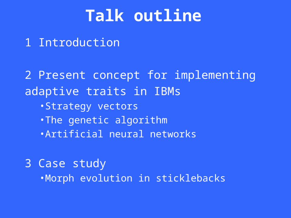
Talk outline

1 Introduction

2 Present concept for implementing adaptive

traits in IBMs•Strategy vectors•The genetic algorithm•Artificial neural networks

3 Case study•Morph evolution in sticklebacks

Life is a lot easier without it..

But

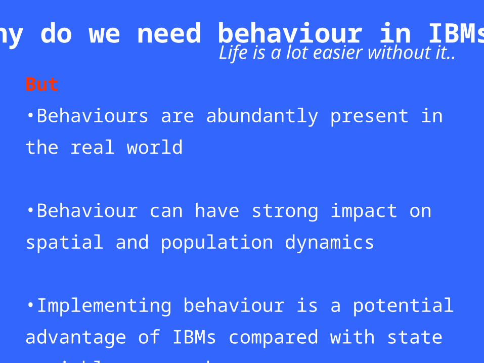
•Behaviours are abundantly present in the real world

•Behaviour can have strong impact on spatial and

population dynamics

•Implementing behaviour is a potential advantage of

IBMs compared with state variable approaches

Why do we need behaviour in IBMs?

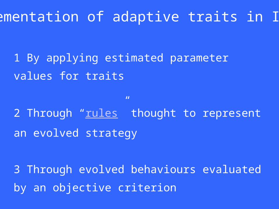
1 By applying estimated parameter values for traits

2 Through “rules” thought to represent an evolved

strategy

3 Through evolved behaviours evaluated by an

objective criterion

Implementation of adaptive traits in IBMs:

Attribute vector: (weight, age,position,fitness,….)

Chambers 1993

Strategy vector: (parity, SAM, allocation of energy, behavioural strategies,...)

Huse et al. (2002)

Specififying individuals in IBMs:

”mum” ”dad” ”offspring”0.56 0.86 0.566.78 5.01 6.785.15 -0.25 5.151.65 1.65 1.85-0.21 0.50 0.508.91 7.56 7.56-2.93 -1.05 -1.05. . .. . .. . .. . .

Breakpoint

The genetic algorithm (Holland 1975)

Strategy vector or ”chromosome”

Mutation

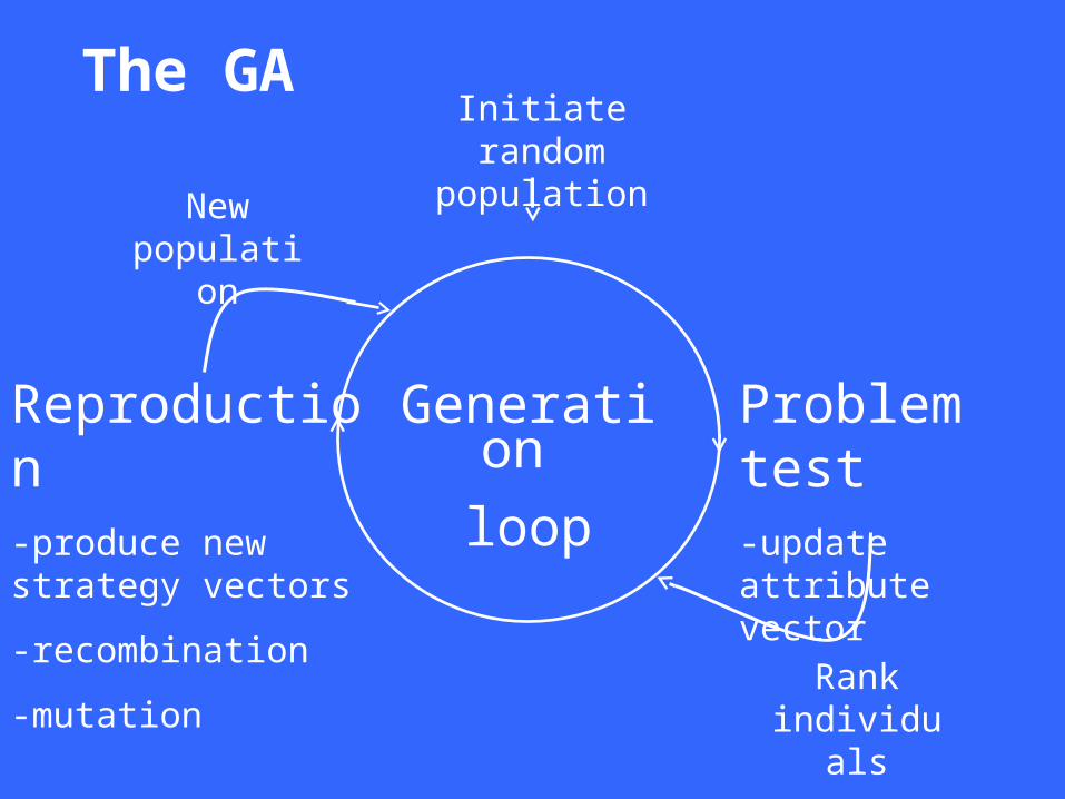
Reproduction-produce new strategy vectors

-recombination

-mutation

The GAInitiate random

population

Problem test-update attribute vector

New population

Generation

loop

Rank individuals

Artificial neural networks can be used to translate strategy vectors into behaviour

Input 1

Input 2

.

.

.

Input n

• Behaviour

•

•

•

Input Hidden Output

Wih

Who

Weights implemented on strategy vector S

Determine by a fitness measure:

•Net reproductive rate R0

•Instantaneous rate of increase r

These fitness measures are hampered by many assumptions and are often difficult to implement in IBMs

•Alternatively: use endogenous fitness

What is a good strategy vector?

Do the GA find optimal solutions?

While optimality models always find the best solution to problems,

How about adaptation models ...?

•Patch choice model

•A simple vertical migration scenario

In cases were the optimal solution can be calculated, it tends to be found by the GA

Exploring adaptive radiation and speciation in fish by individual-

based models(Huse & Hart in prep.)

(Gasterosteus aculeatus)

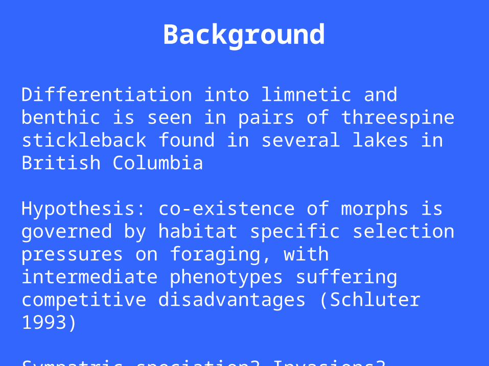
Background

Differentiation into limnetic and benthic is seen in pairs of threespine stickleback found in several lakes in British Columbia

Hypothesis: co-existence of morphs is governed by habitat specific selection pressures on foraging, with intermediate phenotypes suffering competitive disadvantages (Schluter 1993)

Sympatric speciation? Invasions? ..

Objectives

Develop individual-based model of trophic interactions between stickleback morphotypes

Study the effect of diffent prey types, competition, spatial detail and invasions on speciation

Evaluate individual-based modelling as a tool in studying speciation

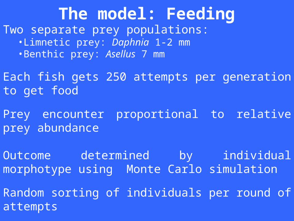
The model: FeedingTwo separate prey populations:

•Limnetic prey: Daphnia 1-2 mm•Benthic prey: Asellus 7 mm

Each fish gets 250 attempts per generation to get food

Prey encounter proportional to relative prey abundance

Outcome determined by individual morphotype using Monte Carlo simulation

Random sorting of individuals per round of attempts

Prey is removed from population when eaten

Growth calculated by bioenergetics

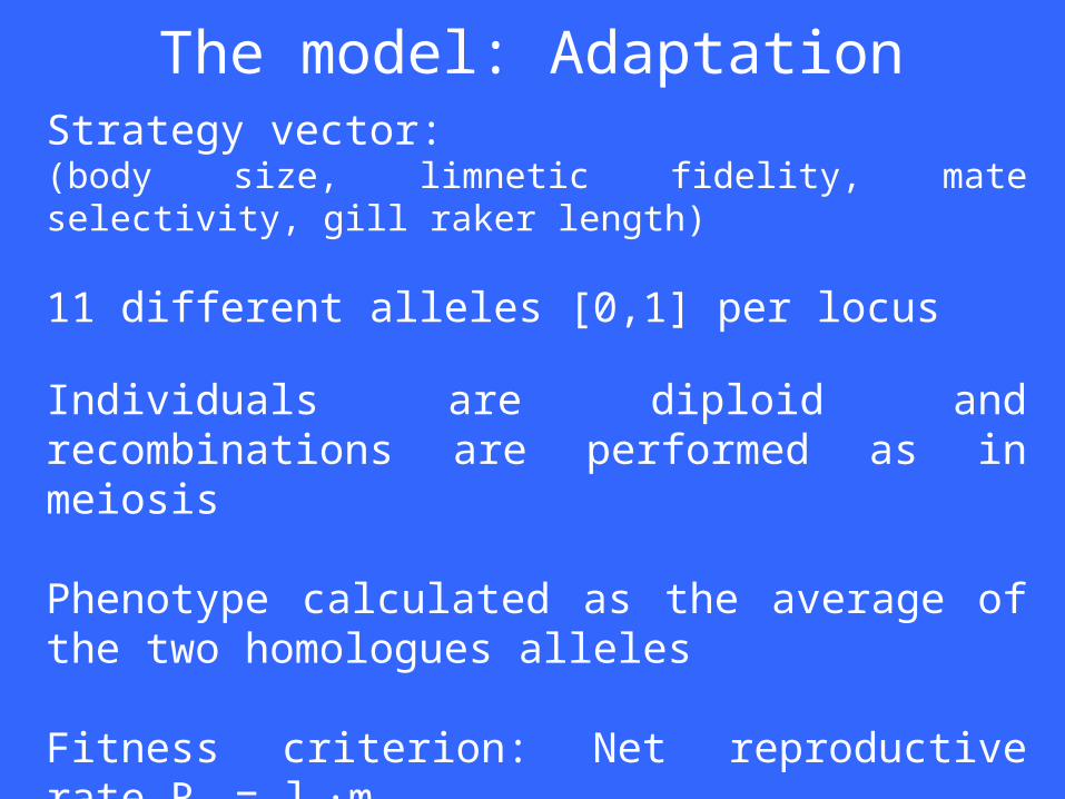
The model: AdaptationStrategy vector:(body size, limnetic fidelity, mate selectivity, gill raker length)

11 different alleles [0,1] per locus

Individuals are diploid and recombinations are performed as in meiosis

Phenotype calculated as the average of the two homologues alleles

Fitness criterion: Net reproductive rate R0 = lx·mx

Offspring production in proportion to fitness

Simulations

Four different simulations are presented: •1 Adaptation without competition

•2 Adaptation with competition

•3 Assortative mating without spatial detail

•4 Assortative mating and spatial detail

General resultsTraining decomposition:

•Individuals act ”silly” due to random initiation of strategies

•Solved by gradually making tasks more difficult

0

200

400

600

800

1000

1200

0 50 100 150 200

Generation

Po

pu

latio

n a

bu

nd

an

ce

0

0.002

0.004

0.006

0.008

0.01

0.012

Fe

cud

ity fa

cto

r

Population size Fecundity factor

1 Adaptation without competition:

Phenotypic differentiation due to different prey sizes available

Gill raker size

0.0

0.1

0.2

0.3

0.4

0.5

0.6

0.7

0.8

0.9

1.0

0.07 0.15 0.22 0.29 0.36 0.44 0.51 0.58 0.65 0.73 0.80

Gill raker length (mm)

Pro

port

ion

Benthic Limnetic Both

0.0

0.1

0.2

0.3

0.4

0.5

0.6

0.7

0.8

0.9

1.0

25 28 31 34 37 40 43 46 49 52 55

Body size (mm)

Pro

port

ion

Benthic Limnetic Both

Body size

2 Adaptation with competition:

Phenotypic differentiation from competition

0.0

0.1

0.2

0.3

0.4

0.5

0.6

25 28 31 34 37 40 43 46 49 52 55

Body size (mm)

Pro

po

rtio

n

Both B-50% B-75% B-85%

Reduced benthic food Reduced limnetic food

0.0

0.1

0.2

0.3

0.4

0.5

0.6

25 28 31 34 37 40 43 46 49 52

Body size (mm)

Pro

po

rtio

n

Both L-50% L-75%

3 Assortative mating without spatial detail

No population divergence seen despite increased competition and assortative mating

Body size

0

0.1

0.2

0.3

0.4

0.5

0.6

25 28 31 34 37 40 43 46 49 52 55

Body Size

Fre

qu

enc

y

Gill raker length

0

0.1

0.2

0.3

0.4

0.5

0.6

0.7

0.8

0.9

0.07 0.22 0.36 0.51 0.65 0.80

Gill raker length

Fre

qu

en

cy

4 Assortative mating and spatial detail

0

0.1

0.2

0.3

0.4

0.5

25 28 31 34 37 40 43 46 49 52 55

Body size (mm)

Fre

qu

en

cy

1

0

0.1

0.2

0.3

0.4

0.5

25 28 31 34 37 40 43 46 49 52 55

Body size (mm)

Fre

qu

en

cy

5

0

0.1

0.2

0.3

0.4

0.5

25 28 31 34 37 40 43 46 49 52 55

Body size (mm)

Fre

qu

en

cy

10

0

0.1

0.2

0.3

0.4

0.5

25 28 31 34 37 40 43 46 49 52 55

Body size (mm)

Fre

qu

en

cy100

0

0.1

0.2

0.3

0.4

0.5

25 28 31 34 37 40 43 46 49 52 55

Body size (mm)

Fre

qu

en

cy

50

0

0.1

0.2

0.3

0.4

0.5

25 28 31 34 37 40 43 46 49 52 55

Body size (mm)

Fre

qu

en

cy

20

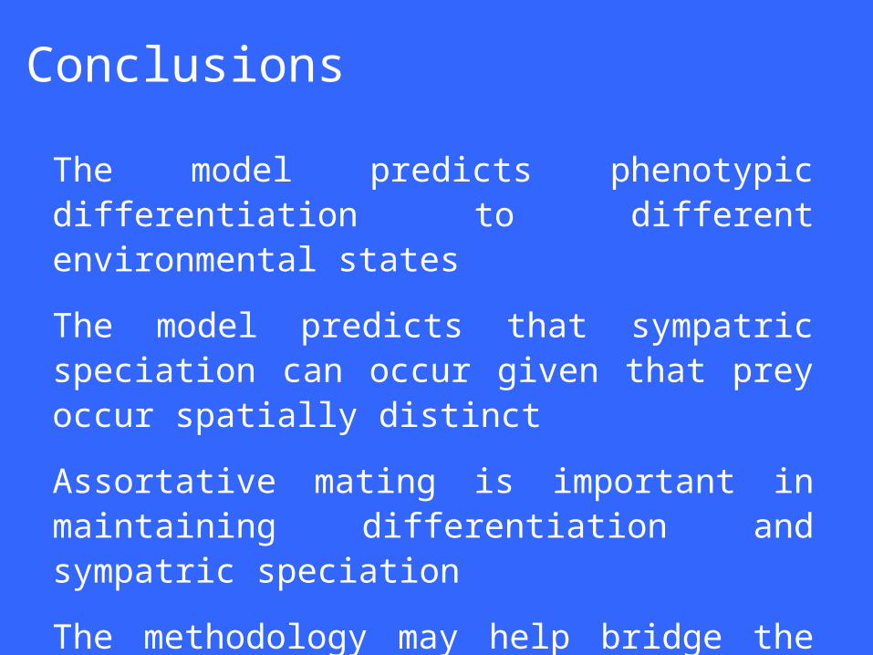
The model predicts phenotypic differentiation to different environmental states

The model predicts that sympatric speciation can occur given that prey occur spatially distinct

Assortative mating is important in maintaining differentiation and sympatric speciation

The methodology may help bridge the gap between phenotypic and genotypic approaches to life history evolution

Conclusions

ANN calculationsVariable description Ii : input data i, Wih : the connection weight between input data i and hidden node h Nh : the sum of the weighted input data of hidden node h m : the number of input nodes connected to hidden node h n : the number of hidden nodes TNh : the transformed node value Bh : the bias Who : the connection weight between hidden node h and output node o

Summing over hidden node h

1mih ih iN W I 1

Transforming hidden node value

)1(

1)( hh BNh

eTN

2

Summing over output node o

1nh ho hO W TN 3

Transforming the output node

( )

1

(1 )oO BTO

e

4

The patch choice model of Mangel and Clark 1988 by ANN

(Huse, Strand & Giske 1999)

•The problem is to find the patch at each time step that maximises the survival to the horizon

given the current state of the individual

SDP ING

Average patch value 2.28 2.30±0.02

Survival 0.51 0.51±0.00

Patch choice similarity (%) 100.0 96.8±1.95

0

10

20

30

40

50

60

70

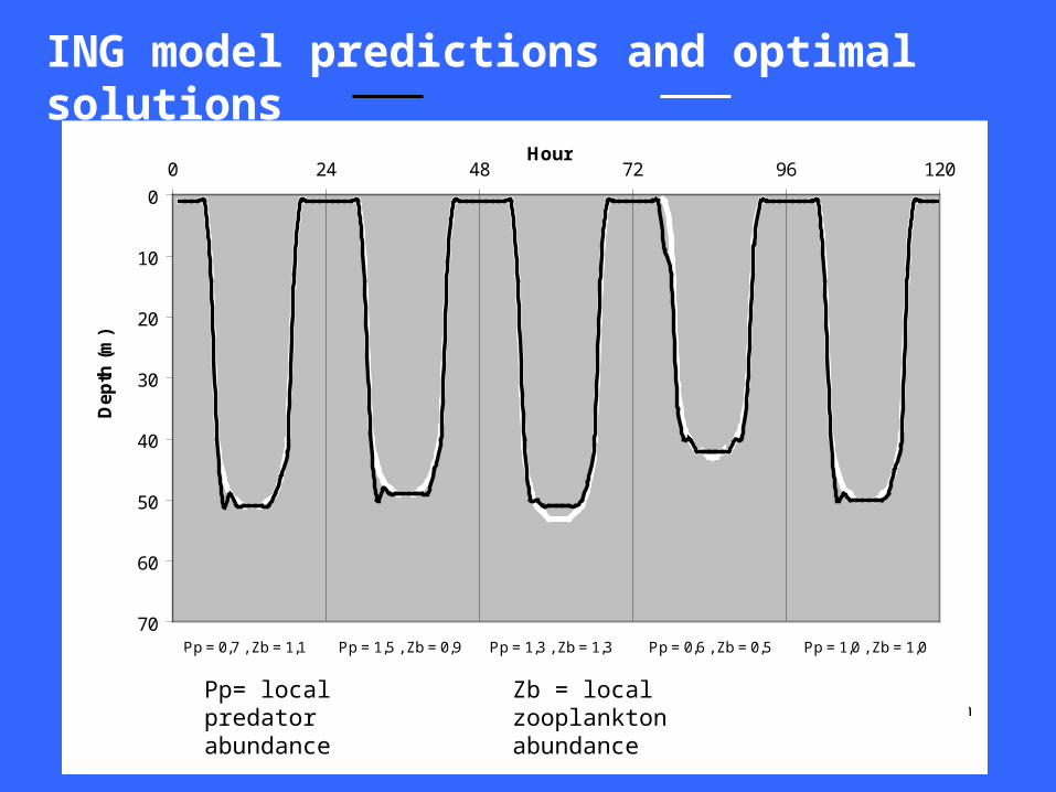
0 24 48 72 96 120Hour

De

pth

(m

)

Pp = 0,7 , Zb = 1,1 Pp = 1,5 , Zb = 0,9 Pp = 1,3 , Zb = 1,3 Pp = 0,6 , Zb = 0,5 Pp = 1,0 , Zb = 1,0

Figure 18: Adapted behaviour in an ING model with a 5:30:1 ANN. The predator density parameter (Pp) and zooplankton biomassparameter (Zb) values are shown for each day at the x-axis. The white line is the global optimum calculated by using the optimisationmodel. Black line is the adapted behaviour of M. muelleri in the ING model. M. muelleri clearly adapts to the stochastic environmentand reaches the global optimum solution.

ING model predictions and optimal solutions

Pp= local predator abundance

Zb = local zooplankton abundance

Makes decision using probability and random numbers

Example

IF random number < probability of getting prey THEN prey is caught

Monte Carlo simulation:

no yes

yes no

no

Get next individual

Feed? Starve?

Preyavailability

Predator field

Eaten?

Calculate encounterrate with predatorsand probability ofbeing captured

Calculate growthand new larval size

Calculate preyencounter rate and

feeding

Add to individualssurviving to next

time step

yes

Record predationmortality

Recordstarvationmortality

Monte Carlo

simulations

•Simulating ”survival of the fittest” within the

model domain

•Monte Carlo simulations

•Those who manage to fulfil the criteria for

reproduction in the best way are the fittest

•Survivors at any time are the fittest

•No knowledge of optimal strategy

Endogenous fitness