11Implicit Functions

11.1 Partial derivatives

To express the fact that z is a function of the two independent variables x and y we writez = z(x, y). If variable y is fixed, then z becomes a function of x only, and if variable x isfixed, then z becomes a function of y only. The notation ∂z/∂x, pronounced ’partial z withrespect to x’, is the derivative function of z with respect to x with y considered a constant.Similarly, ∂z/∂y is the derivative function of z with respect to y, with x held fixed. In anyevent, unlike dy/dx, the partial derivatives ∂z/∂x and ∂z/∂y are not fractions. For the sakeof notational succinctness the partial derivatives may be written as zx and zy.

Examples.

1. For z = x2 + x3y−1 + y3 − 2x + 3y − 5 we have

∂z

∂x= 2x + 3x2y−1 − 2,

∂z

∂y= x3(−y−2) + 3y2 + 3.

2. For z =√

1 + x2y3 we have

∂z

∂x=

2xy3

2√

1 + x2y3,

∂z

∂y=

3y2x2

2√

1 + x2y3.

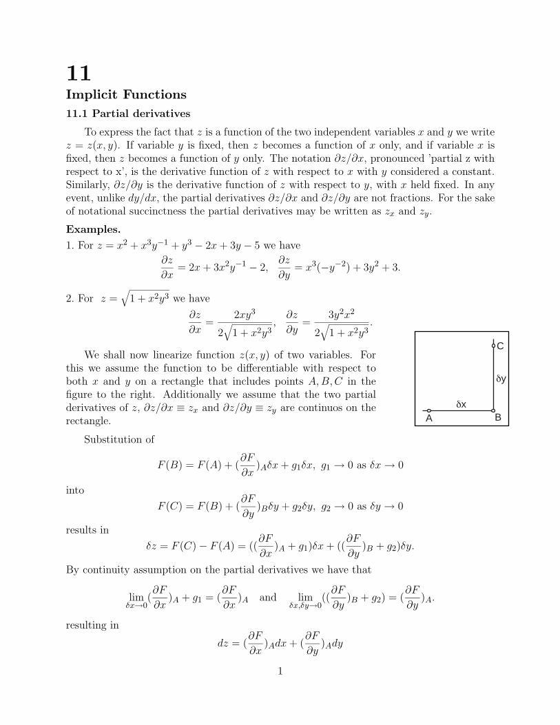
We shall now linearize function z(x, y) of two variables. Forthis we assume the function to be differentiable with respect toboth x and y on a rectangle that includes points A,B,C in thefigure to the right. Additionally we assume that the two partialderivatives of z, ∂z/∂x ≡ zx and ∂z/∂y ≡ zy are continuos on therectangle. A B

C

δx

δy

Substitution of

F (B) = F (A) + (∂F

∂x)Aδx + g1δx, g1 → 0 as δx → 0

into

F (C) = F (B) + (∂F

∂y)Bδy + g2δy, g2 → 0 as δy → 0

results in

δz = F (C) − F (A) = ((∂F

∂x)A + g1)δx + ((

∂F

∂y)B + g2)δy.

By continuity assumption on the partial derivatives we have that

limδx→0

(∂F

∂x)A + g1 = (

∂F

∂x)A and lim

δx,δy→0((∂F

∂y)B + g2) = (

∂F

∂y)A.

resulting in

dz = (∂F

∂x)Adx + (

∂F

∂y)Ady

1

Chapter 11

which is the equation of a plane.

11.2 Implicit Functions

The totality of points (x, y) satisfying the equation F (x, y) = 0 forms a curve. Given avalue of the independent variable x, evaluation of y, supposing one exists, may require theapproximate solution of F (x, y) = 0 by numerical means, such as the method of bisectionsor the metod of successive linearizations. It is possible that for one given x value there isa number of corresponding y values. Yet, it may happen that a restricted portion of theplane delineated by a (finite or infinite) rectangle contains an arc of thetotal curve that is the graph of some function y = y(x). We say thenthat F (x, y) = 0 is an implicit representation of the function y = y(x).The figure to the right shows the tilted ψ shaped curve implicit in someF (x, y) = 0. Intersection point B of the linear and parabolic branchesof the curve is often referred to as a bifurcation point since the curvebranches or forks at such a pont. The figure also shows three rectanglessuch that for any x in a rectangle there is only one corresponding y(x)in the same rectangle, and the three arcs within the three rectanglesshown are thus each the graphs of a function.

B

Examples.

1. The curve described by the equation F (x, y) = y2−2yx2 +x4 = 0 is the parabola y = x2,a fact discovered by observing that F (x, y) = (y−x2)2 = 0. Hence F (x, y) = 0 is the implicitrepresentation of the (explicit) function y(x) = x2.

2. The curve of the equation F (x, y) = x2 + y2 = 0 consists of the single point (0, 0).

3. The curve of F (x, y) = x2 + y2 + 1 is empty. Not one (real) pair (x, y) is found to satisfythis equation.

4. The curve of the equation F (x, y) = x2 − y2 = (x − y)(x + y) = 0 consists of theunion of the two lines y = x and y = −x. The intersection point (0, 0) of the two linesis a bifurcation point. Under the restriction y ≥ 0 the equation F (x, y) = 0 becomes theimplicit representation of the sole explicit function y(x) = |x|, and under the restrictiony ≤ 0 the same equation F (x, y) = 0 becomes the implicit representation of the (single)explicit function y(x) = −|x|5. The curve shown to the right is the locus of the totality of points satisfying

F (x, y) = x4 + 10x2y2 + 9y4 − 13x2 − 45y2 + 36 = 0.

It consists of the union of a circle and an ellipse, as in fact,

F (x, y) = G(x, y)H(x, y) = (x2 + y2 − 4)(x2 + 9y2 − 9).

The combined grapf of the circle and the ellipse shows four points of bifurcation.

6. The curve of the equation

F (x, y) = (x2 + y2)2 − 3(x2 + y2) + 2 = 0

2

Chapter 11

consists of two concentric circles as shown in the figure to the right,a fact discovered by observing that

F (x, y) = (x2 + y2)2 − 3(x2 + y2) + 2 = (x2 + y2 − 1)(x2 + y2 − 2).

1

2

7. The curve described by the equation

F (x, y) = x2 + y2 − 1 = 0, −1 ≤ x ≤ 1

is a full circle, which we may consider as consisting of two branches: an upper half circle anda lower half circle, represented by the two continuous functions, written explicitly as

y1(x) =√

1 − x2 and y2(x) = −√

1 − x2

which are moreover differentiable both on −1 < x < 1. Under the additional restrictiony ≥ 0 the equation F (x, y) = 0 becomes the (unique) implicit representation of the functiony1(x) only, and under the additional restriction y ≤ 0 the equation F (x, y) = 0 becomes the(unique) implicit representation of the function y2(x) only.

Relinquishing continuity, the equation F (x, y) = 0 may be theimplicit representation of a host of other, discontinuous, functionslike the one chosen at random and shown in the figure to the right.Here y(x) ≥ 0 if −1 ≤ x < −0.4 and 0.4 < x ≤ 1; and y < 0 if−0.4 ≤ x ≤ 0.4.

–1

–1 –0.4 0.4 1

1

8. The graph of the equation

F (x, y) = x2 + xy + y2 − 3 = 0 (1)

consists of the union of two curves explicitly described by the two functions

y1(x) =1

2(−x +

√12 − 3x2), y2(x) =

1

2(−x−

√12 − 3x2) (2)

which are continuous on −2 ≤ x ≤ 2 and differentiable on −2 < x < 2. See the figure below.

–2

–10

1

2

–2 –1 1 2

y1(x)

y2(x)

A B

C D

A B

C D

–2

–1

0

1

2

–2 –1 1 2

With the restrictions −2 ≤ x ≤ 1, 1 ≤ y ≤ ∞ the equation F (x, y) = 0 becomes theimplicit representation of the sole function y = y(x) with the graph in the box ABCD inthe figure above to the left. By the restrictions −1 ≤ x ≤ 2, −1 ≤ y ≤ −∞ the equation

3

Chapter 11

F (x, y) = 0 becomes the implicit representation of the sole function y = y(x) with the graphin the box ABCD in the figure above to the right.

We were able to produce the two explicit differentiable functions y1(x) and y2(x) out ofimplicit expression (1) because for any fixed x expression (1) reduces to a mere quadraticequation for y which can be solved by simple and formal algebraic means.

9. consider the function F (x, y) = ey + x2 − 1 = 0. We rewrite the equation as ey = 1 − x2

and restrict x to (−1, 1) and conclude that y = ln(1 − x2) is the sole explicit solution ofF (x, y) = 0.

10. If we choose in the equation

F (x, y) = xey + yex + x2 + y2 − 9 = 0

x = 1, then we are left with the transcendental equation ey + y + y2 − 8 = 0 which canbe solved for y but numerically and approximately. Now, even if F (x, y) = 0 is an implicitrepresentation of the explicit y(x), near x = 1, there is no way this equation can be writtenexplicitly in terms of elementary functions.

Before entertaining some general arguments, we shall theoretically demonstrate that theequation F (x, y) = y5 + y − x + 1 = 0 is an implicit representation of one single functiony = f(x) for any x, inspite of the fact that it can not be turned explicit by any algebraicmeans. Indeed, for any x the equation F (x, y) = 0 is a polynomial equation of odd degreein y and possesses at least one real root. Since ∂F/∂y = 5y4 + 1 > 0 the function F (x, y) isincreasing for any fixed x and F (x, y) = 0 only once. If |x| >> 1, then y = 5

√x, nearly.

Definition Let F (x, y) = 0 is defined in the rectangle a ≤ x ≤ b, a′ ≤ y ≤ b′. Weshall say that F (x, y) = 0 is an implicit representation of y = f(x) in the rectangle, if forany a ≤ x ≤ b there is a single a′ ≤ y ≤ b′, such that the pair x, y satisfies the equationF (x, y) = 0.

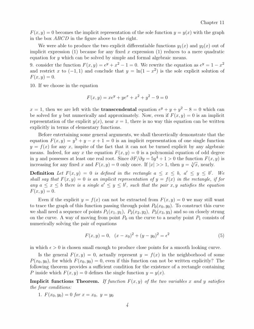
Even if the explicit y = f(x) can not be extracted from F (x, y) = 0 we may still wantto trace the graph of this function passing through point P0(x0, y0). To construct this curvewe shall need a sequence of points P1(x1, y1), P2(x2, y2), P3(x3, y3) and so on closely strungon the curve. A way of moving from point P0 on the curve to a nearby point P1 consists ofnumerically solving the pair of equations

F (x, y) = 0, (x− x0)2 + (y − y0)

2 = ε2 (5)

in which ε > 0 is chosen small enough to produce close points for a smooth looking curve.

Is the general F (x, y) = 0, actually represent y = f(x) in the neighborhood of someP (x0, y0), for which F (x0, y0) = 0, even if this function can not be written explicitly? Thefollowing theorem provides a sufficient condition for the existence of a rectangle containingP inside which F (x, y) = 0 defines the single function y = y(x).

Implicit functions Theorem. If function F (x, y) of the two variables x and y satisfiesthe four conditions:

1. F (x0, y0) = 0 for x = x0, y = y0

4

Chapter 11

2. F (x, y) is continuous in some neighborhood of x = x0, y = y0, that is to say,F (x, y) → F (x0, y0) as x → x0 and y → y0

3. The partial derivatives Fx and Fy of F exist and are continuous in some neighborhoodof x = x0, y = y0

4. Fy(x0, y0) �= 0

then there is a neighborhood of point (x0, y0) in which there is one and only one contin-uous and differentiable function y = f(x), y0 = f(x0), that satisfies F (x, f(x)) = 0.Derivative function f ′(x) of the implicit function is continuous and is given by f ′(x) =−Fx(x, y)/Fy(x, y) with y = f(x).

F=0

F>0

F<0

F>0

F<0

Fy>0

F=0C

δxδy

A B

P Q

R S

Proof. Refer to the figure above in which the sides of the rectangle PQRS are parallel tothe x and y axes. Assume that the function F (x, y) satisfies the conditions of the theoremin and on the rectangle. At point A the partial derivative Fy �= 0 and we assume that(∂F/∂y)A > 0. Function F (x, y) is thus increasing with y, and on some interval above pointA, say up to point R, F > 0, and in some interval below point A, say up to pint P , F < 0.The continuity of F along x implies the existence of δx such that F (S) > 0 and F (Q) < 0.The continuity of F along y implies that F = 0 at point C strictly between S and Q. By theassumption that Fy > 0 on the rectangle, F = 0 on the side QS only once. Implicit functiony = f(x) is the y coordinate of point C.

We will show now that y(x) is differentiable at point A and similarly that the functionis differentiable at any other intermediate point on the curve. Using the fact that F (A) =F (C) = 0 we obtain from the previous paragraph that

0 = (∂F

∂x)A + (

∂F

∂y)B

δy

δx+ g1 + g2

δy

δx.

The continuity assumption on the partial derivatives implies that

limδx→0

(∂F

∂y)B = (

∂F

∂y)A

5

Chapter 11

and

(∂F

∂x)Adx + (

∂F

∂y)Ady = 0

or y′(x) = −(∂F/∂x)/(∂F/∂y). Derivative function y′(x) is continuous since it consists ofthe ratio of two continuous functions with Fy �= 0. Function y(x) is differentiable at pointA and is therefore also continuous there. End of proof.

Examples and counterexamples.

1. For y2 − x = 0 we obtain by implicit differentiation 2yy′ − 1 = 0 leading to the absurdity0 = −1 if x = y = 0 because the function y =

√x is not differentiable at x = 0.

2. For (x− y)2 = x2 − 2xy + y2 = 0 we obtain by implicit differentiation (x− y)(1− y′) = 0and y′ = 1 if x− y �= 0. Actually y = x and y′ = 1 for any x.

3. Expression (x−y)(x+y) = x2−y2 = 0 represents two orthogonal lines through x = y = 0.By implicit differentiation x−yy′ = 0 and at x = y = 0 we get 0 = 0 because of the ambiguityof the bifurcation.

4. Expression x2 + y2 = 0 represents the mere point x = y = 0. By implicit differentiationx + yy′=0, and at x = y = 0 this reduces to 0 = 0.

5. The equation F (x, y) = y3 − x3 = 0 is equivalent to y = x for any x. We have here that3y2y′ − 3x2 = 0 which reduces to 0 = 0 at P (0, 0).

6. ConsiderF (x, y) = x3y + xy3 + x + y − 4 = 0.

Recalling the chain rules (y2)′ = 2yy′ and (y3)′ = 3y2y′, and diffrentiating both side of theabove equation with respect to x we have

(3x2 + x3y′) + (y3 + 3xy2y′) + 1 + y′ = 0

which is linear in y′, and is readily solved to produce

y′ = −3x2y + y3 + 1

x3 + 3xy2 + 1= −Fx(x, y)

Fy(x, y).

For x = 1, y = 1, that satisfy the present F (x, y) = 0, yields y′(1) = −1

7. For F (x, y) = y3−6xy+5 = 0 we shall compute y′ and y′′ at P (1, 1). From (y3−6xy+5)′ =0 we obtain y2y′ − 2y − 2xy′ = 0, and y′(1) = −2. From (y2y′ − 2y − 2xy′)′ = 0 we obtain2y′y′ + y2y′′ − 4y′ − 2xy′′ = 0, and y′′(1) = 16.

8. Expression x2 + y2 = r2 describes both the upper and the lower arc of a circle centeredat C(0, 0) and having radius r. Repeated differentiation produces here

x + yy′ = 0 and 1 + (y′)2 + yy′′ = 0

so that the critical points of both functions implicit in the equation of the circle happen tobe at x = 0, y = ±r. But if y′ = 0, then y′′ = −1/y, and y′′ = −1/r if y = +r, implying alocal maximum, and y′′ = 1/r if y = −r implying a local minimum.

6

Chapter 11

9. For the function

F (x, y) = G(x, y)H(x, y) = (x2 + y2 − 4)(x2 + 9y2 − 9)

considered before we have

∂F

∂x=

∂G

∂xH + G

∂H

∂xand

∂F

∂y=

∂G

∂yH + G

∂H

∂y

and both ∂F/∂x = 0 and ∂F/∂y = 0 at the bifurcation points at which at once G = H = 0.

Exercises.

1. Find all critical points of the folium of Descartes x3 + y + 3 − 3xy = 0. Ans. y′ =−(x2 − y)/(y2 − x). x0 = 21/3, y0 = 41/3. Max.

2. Show that if f(x+y) = f(x)+f(y) for any x and y, then f(x) = ax for constant a. Hint:First we observe that if x = y = 0, then f(0) = 2f(0), and hence f(0) = 0. We introducethe auxiliary variable u = x+ y, and have upon differentiation with respect to x and y thatf ′(u) = f ′(x) and f ′(u) = f ′(y), or f ′(x) = f ′(y) for any x and y, implying that f ′(x) = afor some constant a. Hence f(x) = ax + b, but b = 0.

3. Show that if function f(x) is such that

f(x + y)f(x− y) = f2(x) − f2(y)

for any x and y, then f(0) = 0, and f ′′(x)/f(x) =constant. Hint: Set in the above equationx = (u + v)/2, y = (u− v)/2 and differentiate it twice with respect to u and v.

4. Prove that if differentiable function f(u) is such that f(x + y) = f(x) + f(y) for any xand y, then f ′(x) = f ′(y) for any x and y.

5. Prove that if differentiable function f(u), u > 0 is such that f(xy) = f(x) + f(y) for anypositive x and y, then xf ′(x) = yf ′(y) for any positive x and y.

6. Prove that if differentiable function f(u) is such that f(x + y) = f(x)f(y) for any x andy, then f ′(x)/f(x) = f ′(y)/f(y) for any x and y.

7. For what function does it happen that f(xy) = f(x)f(y)?

11.3 Tracking an implicit curve

Pursuing an implicit differentiable curve, or trajectory, entails placing close points on it.Presented here is a leap-and-land algorithm for doing that. Let F (x, y) = 0 be the implicitequation of the curve and let A(x0, y0) be a point on it such that F (A) = 0. The equationof the tangent line to the curve at point A is

(∂F

∂x)Adx + (

∂F

∂y)Ady = 0 or (

∂F

∂x)A(x− x0) + (

∂F

∂y)A(y − y0) = 0

We propose to leap forward from point A and place point B on the tangent line at distanceε from A. Point B is close to the curve (one must beware, though, of the danger of jumpingfrom one branch of the function to another that may happen to be nearby) and from it wewill attempt a short distance return that will land us back on the curve.

7

Chapter 11

The tangential leap is restricted to distance ε with dx2 + dy2 = ε2, resulting in

dx = εFy√

F 2x + F 2

y

, dy = −εFx√

F 2x + F 2

y

(1)

with the signs chosen to produce a clock-wise tracking, and with the partial derivativesevaluated all at point A. For instance, if F (x, y) = x2 + y2 − 1, then Fx = 2x, Fy = 2y,and dx = εy0 and dy = −εx0. A tangential leap originating at A(x0, y0) terminates at pointB(x0 + εy0, y0 − εx0). Look an the figure below.

εA

B

C

F=0

F=F(B)

(Fx)A dx+(Fy)A dy=0

(Fx)B dx+(Fy)B dy=0

(Fy)B dx-(Fx)B dy=0

We consider point B(x1, y1) as situated on the curve F (x, y) = F (B) = F (x1, y1) havingthe tangent line

(∂F

∂x)Bdx + (

∂F

∂y)Bdy = 0 or (

∂F

∂x)B(x− x1) + (

∂F

∂y)B(y − y1) = 0.

Point C is the intersection point of the line orthogonal to this tangent line and the curveF = 0. To reach point C from point B we need the corrections dx and dy such that

F (x1 + dx, y1 + dy) = 0 under the restriction that (Fy)Bdx− (Fx)Bdy = 0.

This system of equations is solved approximately by the linearization

F (x1 + dx, y1 + dy) = F (x1, y1) + (Fx)Bdx + (Fy)Bdy = 0

to yield

dx = − F

F 2x + F 2

yFx, dy = − F

F 2x + F 2

yFy

in which function F and its partial derivatives Fx and Fy are evaluated at point B(x1, y1).

If |F (C)|, evaluated at C(x1 + dx, y1 + dy), is less than some prescribed tolerance, thena new leap is executed and a new landing on the curve attempted. If |F (C)| is deemed notsufficiently small, then point C is taken instead of point B and the linearization is repeated.

8

Chapter 11

The above figure shows a fourteen-step tracking of the unit circle F (x, y) = x2 + y2 − 1by linear leaps of ε = 0.49 and a single orthogonal correction.

11.4 The osculating line and circle

Let the equation F (x, y) = 0 be the implicit representation of the function y = f(x),which we assume twice differentiable around some point P on its curve. The equation of thetangent (osculating) line to the graph of the function at point P (x1, y1) on the curve is

(x− x1)(Fx)1 + (y − y1)(Fy)1 = 0

in which, for short, Fx = ∂F/∂x and Fy = ∂F/∂y, and where the subscript 1, refers toevaluations at point P (x1, y1). Subsequently we will drop the subscript 1 for notationalneatness. The line is said to be osculating1 to the graph since y(x1) and y′(x1) for the lineare the same as for the function.

To obtain y′′(x) for the implicit function we start with

dF = 0 = Fx dx + Fy dy or G =dF

dx= 0 = Fx + Fyy

′

and proceed to obtain

dG

dx=

d2F

dx2= 0 =

dFx

dx+

d(Fyy′)

dx=

dFx

dx+

dFy

dxy′ + Fyy

′′

and consequently0 = Fxx + Fxy + (Fyx + Fyyy

′)y′ + Fyy′′.

Assuming that Fxy = Fyx and using y′ = −Fx/Fy we obtain the second derivative in termsof the partial derivatives as

y′′ =−FxxF

2y + 2FxyFxFy − FyyF

2x

F 3y

.

We write the equation of the general circle

(x− x0)2 + (y − y0)

2 = r2

1 Related to scale, to mount, to climb up, to cover

9

Chapter 11

and repeatedly differentiate it to have

(x− x0) + (y − y0)y′ = 0 and 1 + y′2 + (y − y0)y

′′ = 0

from which we obtain the center C(x0, y0) and radius r as

x0 = x− 1 + y′2

y′′y′, y0 = y +

1 + y′2

y′′r =

(1 + y′2)3/2

|y′′| .

Putting into the above expressions y′ and y′′ of any function we obtain the center and radiusof the osculating circle to the curve at point P (x, y) on it. If the function is given implicitlyas F (x, y), then in terms of the partial derivatives

x0 = x +F 2x + F 2

y

∆Fx y0 = y +

F 2x + F 2

y

∆Fy r =

√F 2x + F 2

y

|∆|∆ = −FxxF

2y + 2FxyFxFy − FyyF

2x .

Examples.

1. If f(x) = x2, then f ′(x) = 2x and f ′′(x) = 2. For this parabola

x0 = −x3, y0 =1

2(1 + 6x2), and r =

1

2(1 + 4x2)3/2.

In particular, if x = 0, then x0 = 0, y0 = 1/2, and r = 1/2.

2. Take F (x, y) = y2 − x and P (0, 0). Here, at P

Fx = −1, Fy = 0 Fxx = 0, Fxy = 0, Fyy = 2 ∆ = −2

so thatx0 = 1/2, y0 = 0, r = 1/2

and the osculating circle is as in the figure below.

y=√x

(x-1/2)2+y2=1/4

0

vertical tangent line

In the tracking algorithm of the previous section instead ofleaping from point A on the curve to point B nearby, moving onthe tangent line, we could proceed along an arc of the osculatingcircle to be even closer to the curve before attempting to land onit.

Consider the figure below to the right. Geometrically, we myconstruct the osculating circle this way. The center of a circle, andconsequently its radius is found at the intersection of two normals.Let the arc in the figure to the right be the graph of function f ,twice differentiable in some neighborhood of x1. A small portion of the bent arc betweenpoints A and B appears circular. The two normals raised at point A and B intersect atpoint C. If point C reaches a limit position as B → A, then point C is the center of theosculating circle to the curve at point A.

10

Chapter 11

The coordinates of point C are found from the intersection of the two normals

y − y1 = − 1

y′1(x− x1), y − y2 = − 1

y′2(x− x2)

and

x0 = limx2→x1

(y2 − y1)y′1y

′2 − x1y

′2 + x2y

′1

y′1 − y′2.

Application of L’Hopital’s rule produces the limit values

x0 = x− y′

y′′(1 + y′2), y0 = y +

1

y′′(1 + y′2)

in which the subscript 1 was removed. The radius r of the limit circle is

r = [(x− x0)2 + (y − y0)

2]1/2 =1

|y′′|(1 + y′2)3/2

as before.

x1

y1

x2

y2

slope=-1/y1'

slope=-1/y2'

A

B

C(x0,y0)

The inverse κ = 1/r is called the curvature of the curve at point A,

κ =|y′′|

(1 + y′2)3/2.

For a line κ = 0, and at a corner κ = ∞.

We can obtain the osculating circle also also this way. Letf(x) be twice differentiable at x = 0 and such that f(0) =f ′(0) = 0. The equation of a circle of radius r centered atC(0, r) and passing through O(0, 0) is x2 + (y − r)2 = r2. Theintersection of this circle and f(x) occurs at points O and P .See the figure to the right. At an intersection point y = f(x)and at such a point x2 + (f − r)2 = r2 or

r =x2 + f2

2f.

circle

f(x)

O

P

C(0,r)

of radius r

Letting x → 0, or P → O, and using L’Hopital’s rule we get

limx→0

x2 + f2

2f= lim

x→0

2x + 2ff ′

2f ′= lim

x→0

1 + f ′2 + ff ′′

f ′′=

1

f ′′(0)

which is the radius of the osculating circle at P .

For the function f(x) = (ex + e−x)/2 − 1 this yields r = 1.

11.5 The osculating ellipse

11

Chapter 11

We shall write the equation of the osculating ellipse for a symmetrical function at P (0, 0).In its canonical form the equation of the ellipse is

b2(x− x0)2 + a2(y − y0)

2 = a2b2.

Differentiating the equation repeatedly we obtain the set of four equations

b2(x− x0) + a2(y − b)y′ = 0, b2 + a2y′2 + a2(y − y0)y′′ = 0

3y′y′′ + (y − y0)y′′′ = 0, 3yy′′2 + 4y′y′′′ + (y − y0)y

′′′′ = 0.

For x = 0, y = 0, y′ = 0, y′′ > 0, y′′′ = 0, y′′′′ > 0 theequations are reduced to

x0 = 0, y0 = b, b = 3y′′/y′′′′ and a =√

3/y′′′′.

For the function f(x) = (ex + e−x)/2 − 1 the semi-axes area =

√3, b = 3. See the figure to the right.

3

–2 2

y=(ex+e-x)/2-1

ellipse

circle

0

11.6 From Fixed-point to Newton to Halley to Higher Order Iterations

11.6.1 Fixed point iteration

Definition. Real number a is a fixed point of function f(x) if a = f(a).

The, utterly simple, fixed point iteration method recursively gets xn+1 from xn by xn+1 =f(xn), starting with an initial guess x0. Under certain conditions xn → a, the fixed point off(x), as n → ∞.

The First Fixed Point Iteration Theorem: Let a be a fixed point of f(x). If |f ′(x)| < 1on the open interval I = (a− δ, a+ δ), δ > 0, then the sequence {xn} generated by the fixedpoint iteration xn+1 = f(xn) converges to a, for any initial guess x0 ∈ I.

Proof. Let x0 ∈ I. We write

x1 − a = f(x0) − a = f(x0) − f(a)

apply the mean-value theorem in the form f(x0) = f(a) + (a− x0)f′(ξ), and have

x1 − a = (x0 − a)f ′(ξ) or |x1 − a| = |x0 − a| |f ′(ξ)|

where ξ ∈ I. By virtue of the fact that |f(ξ)| < 1 the next iterant x1 = f(x0) is nearer to athen x0 and is therefore also in I. End of proof.

Example. Consider the linear function f(x) = k(x− a) + a, k �= 1. for which

x1 − a = k(x0 − a).

If k > 0, then x1 − a and x0 − a have the same sign, but if k < 0, then x1 − a and x0 − ahave opposite signs.

12

Chapter 11

See the figure below.

f(x1)

a ax1� x1�x0

�

�f(x1)�

f(x0)�

y=x

y=f(x)y=f(x)f(x0)

x0

Moreover, as |k| becomes smaller, or as the linear function f(x) = k(x − a) + a tilts closerto being horizontal, convergence becomes faster. See the figure below.

a

�

y=f(x)

a

y=f(x)

y=x y=x

In the general case, we expect the fixed point iteration x1 = f(x0) to be fast converging iffunction f(x) is flat and nearly horizontal at x = a. Namely, if f ′(a) = f ′′(a) = · · · = 0,which is the assertion of the next theorem.

The second, general, fixed point theorem: Let a be a fixed point of function f(x), a =f(a). Suppose f(x) has a bounded derivative of order m + 1 in an open interval containingfixed point a. If f ′(a) = f ′′(a) = . . . = f (m)(a) = 0, but f (m+1)(a) �= 0, then the sequencexn produced by the recursion xn+1 = f(xn) is such that |a − xn+1| < c|a − xn|m, for someconstant c > 0, provided that x0 is taken close enough to a.

Proof: We shall prove the theorem for the specific case of m = 2. Let f ′′(x) be bounded onthe interval I = (a− δ, a+ δ), δ > 0, and assume x to be in this interval. Taylor’s expansionof f(x) around point a is

f(x) = f(a) + (x− a)f ′(a) +1

2(x− a)2f ′′(a) +

1

6(x− a)3f ′′′(ξ), a < ξ < x

if x is to the right of a. The assumptions a = f(a), f ′(a) = 0, f ′′(a) = 0 reduce this equalityto f(x)−a = (1/6)(x−a)3f ′′′(ξ) or |f(x)−a| ≤ (M/6)|x−a|3, where M is an upper bound

13

Chapter 11

on |f ′′′(x)| in I. For x1 = f(x0) the inequality becomes

|x1 − a| ≤ c|x0 − a|3, c =M

6

and if |x0 − a| < 1, then |x0 − a|3 is much smaller than one. For x0 sufficiently close to a,x1 is closer to a then x0, and hence it is also in I, and so on. End of proof.

Exercises.

1. If the fixed-point iteration

x1 =x2

0 + x0 + 2

x20 + x0 + 1

, x1 = f(x0)

converges, to what number does it converge? Show that x1 > 0 for any x0. Consider f ′(x)and prove that it converges from any starting point. What is x1 if x0 is very large?

2. If the fixed-point iteration

x1 =x0

1 +√

1 + x20

, x1 = f(x0)

converges, to what number does it converge? Does the scheme converge from any startingpoint? What is x1 if x0 is very large?

3. Study the convergence, or divergence, of

xn = ex0−0.5 − 0.5.

Start from x0 = 0.45, then from x0 = 0.55.

4. Find fixed points a off(x) = αx(1 − x).

For what α is |f ′(a)| < 1?

5. Study the behavior of the fixed point iterates of f(x) = αx(1 − x) for a = 3.45 anda = 3.5699465. Start with x0 only slightly different than the fixed point.

6. Study the behavior of the iterates of x1 = 1−x0+x20. Start with x0 = 0.99 and x0 = 1.01.

7. Study the behavior of the iterates of x1 = 1/(2−x0). Start with x0 = 0.99 and x0 = 1.01.

8. Study the behavior of the iterates of x1 = 1/(2−x0)2. Start with x0 = 0.99 and x0 = 1.01.

9. For what c does f(x) = x2 + c have a fixed point? Study the behavior of the iterates ofxn+1 = f(xn) for c = −1,−1.5 and c = −2. Start with x0 = 0 and carry at least 20 iterativesteps.

10. Apply the fixed point iteration xn+1 = f(xn) to the function f(x) = kx+ (1− k)a with0 ≤ k < 1. Show that xn = kn(x0 − a) + a so that xn → a = f(a) as n → ∞.

Theorem: Let function y = f(x) be continuous and such that for any a ≤ x ≤ b alsoa ≤ y ≤ b (concisely put f : [a, b] → [a, b].) Then f(x) has at least one fixed point c = f(c).

14

Chapter 11

Proof. By the assumptions f(a) ≥ a and f(b) ≤ b, hence according to the IntermediateValue Theorem there exists a number c ∈ [a, b] such that c = f(c). End of proof.

The Banach fixed point theorem: Let I = [a, b] be a closed, finite or infinite, interval.If function f(x) is such that:

1. for any x ∈ I also f(x) ∈ I

2. |f(x) − f(y)| ≤ q|x− y| with 0 ≤ q < 1

Then

1 function f(x) has a unique fixed point a = f(a)

2 for any x0 ∈ I the sequence x0, x1, x2, . . . generated by xn+1 = f(xn) converges to the fixedpoint a.

Remark. Notice that f(x) is not assumed continuous in this theorem.

Proof. To prove uniqueness suppose a �= b are two fixed points of f(x) in I. The assumptionson a and b imply that

|a− b| = |f(a) − f(b)| ≤ q|a− b| < |a− b|

which is a contradiction unless a = b.

We will prove the second part of the theorem by showing that:

1. The sequence {xn}n=∞n=0 generated by xn+1 = f(xn) is a Chaucy sequence and hence

converging to some real a.

2. a ∈ I.

3. a = f(a)

We have that

|xn+1 − xn| = |f(xn) − f(xn−1)| ≤ q|xn − xn−1| ≤ · · · ≤ qn|x1 − x0|.

Also, since xn − x0 = (xn − xn−1) + (xn−1 − xn−2) + · · · + (x1 − x0), then

|xn − x0| ≤ |xn − xn−1| + |xn−1 − xn−2| + · · · + |x1 − x0|

or

|xn − x0| ≤ (qn−1 + qn + · · · + 1)|x1 − x0| =1 − qn

1 − q|x1 − x0|.

Similarily,

|xm − xn| ≤ qn1 − qm−n

1 − q|x1 − x0|, m > n

implying that indeed {xn}n=∞n=0 is a Cauchy sequence which has a limit, say a.

Since x0 ∈ I, then also x1 = f(x0) ∈ I and so on for all xn. Hence a ∈ I.

To prove that a is a fixed point of f(x) assume it is not so, that |f(a)−a| = ε > 0. Sincexn → a, natural number N exists such that |xn − a| ≤ ε/2 for all n ≥ N . But

|f(a) − a| = |(f(a) − xN+1) + (xN+1 − a)| ≤ |f(a) − xN+1| + |a− xN+1|

15

Chapter 11

= |f(a) − f(xN )| + |a− xN+1|≤ q|a− xN | + |a− xN+1| < ε

which is a contradiction, and a is a fixed point of f(x). End of proof.

Theorem: Let a be the fixed point of f(x) under the assumptions of the previous theorem.Then for any natural n

|xn − a| ≤ qn

1 − q|x1 − x0|

or equivalently

|xn+1 − a| ≤ q

1 − q|xn+1 − xn|

and|xn+1 − a| ≤ q|xn − a|.

Proof. From the properties of f(x) and the way xn+1 is obtained from xn we have that

|xn − a| = |f(xn−1 − f(a)| ≤ q|xn−1 − a|≤ q2|xn−2 − a| ≤ · · · ≤ qn|x0 − a|.

But|x0 − a| = |x0 − x1 + x1 − a| ≤ |x0 − x1| + |x1 − a|

≤ |x1 − x0| + q|x0 − a|and

|x0 − a| ≤ 1

1 − q|x0 − x1|.

End of proof.

We briefly consider the appliction of the fixed point iteration to the solution of the linearsystem of equations Ax = f . We write x = x + α(Ax− f), α �= 0 which is equivalent to theoriginal system. How to fix α so that x1 = x0 + α(Ax0 − f) converges, and at a brisk pace,is not a simple matter, but an example will do for now. Take α = 1/2, start with the initialvector x0 = (0, 0) and carry out several iteratios towrd the solution of the linear system oftwo equations in two unknowns[

2 −1−1 2

] [x1

x2

]=

[4−5

], Ax = f, x =

[1−2

].

11.6.2 The Newton-Raphson iteration

Finding the root a of the nonlinear equation f(x) = 0. is equivalent to locating the fixed-point of x = x + g(x)f(x), g(a) �= 0. We write F (x) = x + gf and seek g(x) so thatF ′(a) = 0 to secure, in view of the previous theorem, a quadratic convergence for xn+1 =xn + F (xn). Differentiating F (x) by the product rule we have F ′(x) = 1 + g′f + gf ′, andF ′(a) = 1 + g′f(a) + gf ′(a) = 1 + gf ′(a) since f(a) = 0. Conceding that we do not know

16

Chapter 11

fixed point a we settle for a = xn to have g(xn) = −1/f ′(xn), or in short g = −1/f ′n. Withthis g the fixed-point iteration becomes

xn+1 = xn − fnf ′n

which is the Newton-Raphson method, presently shown to quadratically converge to a simpleroot of f(x) = 0. To prove the quadratic convergence of the NR method we derive it fromthe fixed point iteration by taking F (x) = x+ g(x)f(x), g(x) = A/f ′(x) for constant A, andfix it from F ′(a) = 0 as A = −1 independently of a. For a geometrical interpretation of theNR method see the figure below.

a x1 x0

f(x0)

tangent

x0-x1

f(x0)�x0-x1

=f'(x0)

f(x)

To observe the quadratic convergence of the NR method we select f(x) = x2 − 1 for whichx1 = x0−(x2

0−1)/(2x0), or x1−1 = x0−1−(x20−1)/(2x0) resulting in x1−1 = (1/2x0)(x0−1)2

or x1 − 1 = (1/2)(x0 − 1)2 if x0 = 1, nearly.

Exercises.

1. Show that the Newton-Raphson method converges to the (repeating) root of f(x) = x2 =0 only linearly.

2. Fix constant A so as to make the modified Newton-Raphson method xn+1 = xn −Af(xn)/f ′(xn) converge quadratically to the zero root of the cubic f(x) = a2x

2 + a3x3.

3. Study the convergence of the Newton-Raphson method in locating the root of f(x) = x1/3.

It may happen that even if root a of f(x) = 0 is unknown still f ′(a) is known viaa differential equation for f . Consider using the NR method for computing the naturallogarithm. Here f(x) = ex − α, the root of which is a = lnα, and f ′(a) = α. Usingxn+1 = xn − fn/f

′n we have xn+1 = xn − (exn − α)/exn , while using xn+1 = xn − fn/f

′(a)we have xn+1 = xn − (exn − α)/α.

11.6.3 The Halley iteration

We write x = F (x), F (x) = x + g(x)f(x) so that the fixed point a of F is a rootof f, f(a) = 0, if g(a) �= 0, and we prepare to consider the fixed point iterative methodxn+1 = F (xn). We differentiate F (x) twice to have

F ′(x) = 1 + gf ′ + g′f and F ′′(x) = gf ′′ + 2g′f ′ + g′′f

17

Chapter 11

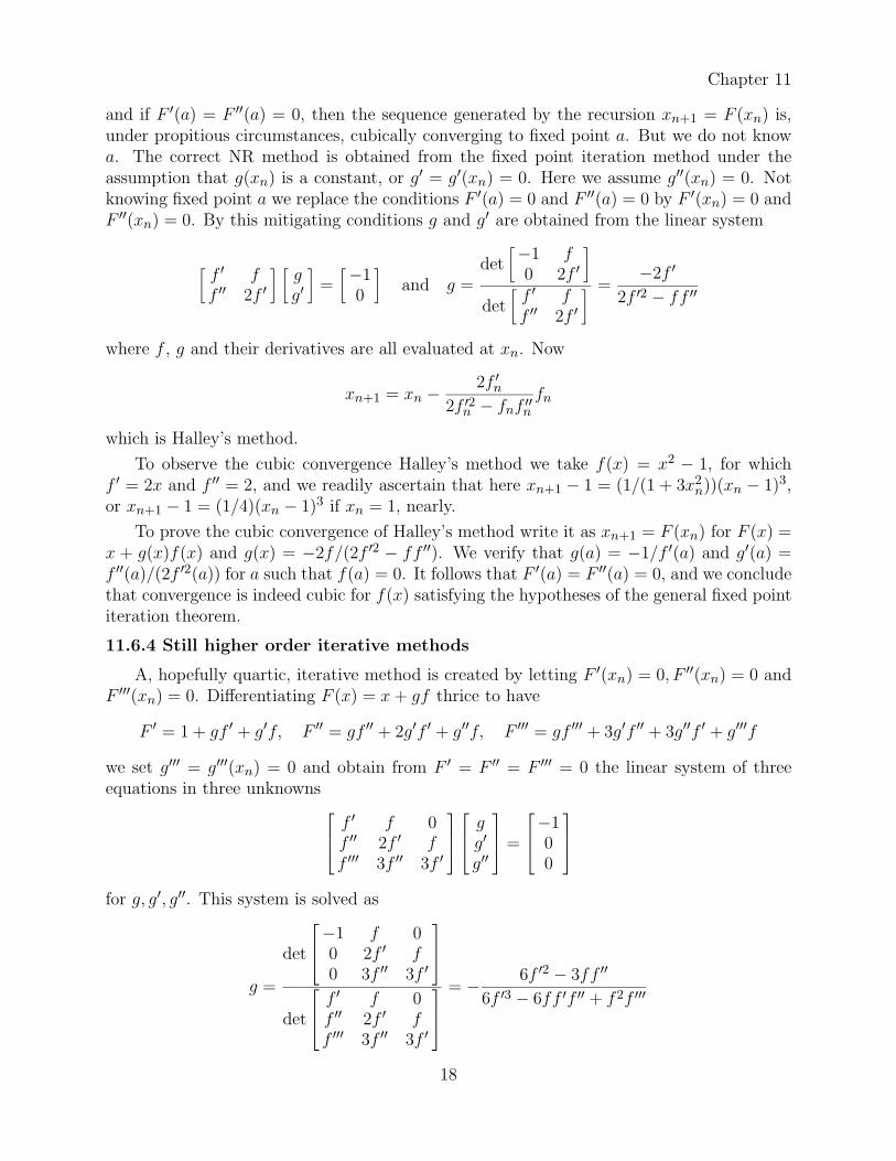
and if F ′(a) = F ′′(a) = 0, then the sequence generated by the recursion xn+1 = F (xn) is,under propitious circumstances, cubically converging to fixed point a. But we do not knowa. The correct NR method is obtained from the fixed point iteration method under theassumption that g(xn) is a constant, or g′ = g′(xn) = 0. Here we assume g′′(xn) = 0. Notknowing fixed point a we replace the conditions F ′(a) = 0 and F ′′(a) = 0 by F ′(xn) = 0 andF ′′(xn) = 0. By this mitigating conditions g and g′ are obtained from the linear system

[f ′ ff ′′ 2f ′

] [gg′

]=

[−10

]and g =

det[−1 f

0 2f ′

]det

[f ′ ff ′′ 2f ′

] =−2f ′

2f ′2 − ff ′′

where f , g and their derivatives are all evaluated at xn. Now

xn+1 = xn − 2f ′n2f ′2n − fnf ′′n

fn

which is Halley’s method.

To observe the cubic convergence Halley’s method we take f(x) = x2 − 1, for whichf ′ = 2x and f ′′ = 2, and we readily ascertain that here xn+1 − 1 = (1/(1 + 3x2

n))(xn − 1)3,or xn+1 − 1 = (1/4)(xn − 1)3 if xn = 1, nearly.

To prove the cubic convergence of Halley’s method write it as xn+1 = F (xn) for F (x) =x + g(x)f(x) and g(x) = −2f/(2f ′2 − ff ′′). We verify that g(a) = −1/f ′(a) and g′(a) =f ′′(a)/(2f ′2(a)) for a such that f(a) = 0. It follows that F ′(a) = F ′′(a) = 0, and we concludethat convergence is indeed cubic for f(x) satisfying the hypotheses of the general fixed pointiteration theorem.

11.6.4 Still higher order iterative methods

A, hopefully quartic, iterative method is created by letting F ′(xn) = 0, F ′′(xn) = 0 andF ′′′(xn) = 0. Differentiating F (x) = x + gf thrice to have

F ′ = 1 + gf ′ + g′f, F ′′ = gf ′′ + 2g′f ′ + g′′f, F ′′′ = gf ′′′ + 3g′f ′′ + 3g′′f ′ + g′′′f

we set g′′′ = g′′′(xn) = 0 and obtain from F ′ = F ′′ = F ′′′ = 0 the linear system of threeequations in three unknowns f ′ f 0

f ′′ 2f ′ ff ′′′ 3f ′′ 3f ′

gg′

g′′

=

−100

for g, g′, g′′. This system is solved as

g =

det

−1 f 00 2f ′ f0 3f ′′ 3f ′

det

f ′ f 0f ′′ 2f ′ ff ′′′ 3f ′′ 3f ′

= − 6f ′2 − 3ff ′′

6f ′3 − 6ff ′f ′′ + f2f ′′′

18

Chapter 11

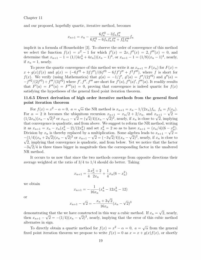
and our proposed, hopefully quartic, iterative method, becomes

xn+1 = xn − 6f ′2n − 3fnf′′n

6f ′3n − 6fnf ′nf ′′n + f2nf

′′′nfn

implicit in a formula of Householder [3]. To observe the order of convergence of this methodwe select the function f(x) = x2 − 1 for which f ′(x) = 2x, f ′′(x) = 2, f ′′′(x) = 0, anddetermine that xn+1 − 1 = (1/(4x3

n + 4xn))(xn − 1)4, or xn+1 − 1 = (1/8)(xn − 1)4, nearly,if xn = 1, nearly.

To prove the quartic convergence of this method we write it as xn+1 = F (xn) for F (x) =x + g(x)f(x) and g(x) = (−6f ′2 + 3ff ′′)/(6f ′3 − 6ff ′f ′′ + f2f ′′′), where f is short forf(x). We verify (using Mathematica) that g(a) = −1/f ′, g′(a) = f ′′/(2f ′2) and g′′(a) =−f ′′2/(2f ′3)+ f ′′′/(3f ′2) where f ′, f ′′, f ′′′ are short for f ′(a), f ′′(a)′, f ′′′(a). It readily resultsthat F ′(a) = F ′′(a) = F ′′′(a) = 0, proving that convergence is indeed quartic for f(x)satisfying the hypotheses of the general fixed point iteration theorem.

11.6.5 Direct derivation of high order iterative methods from the general fixedpoint iteration theorem

For f(x) = x2 − α = 0, a =√α the NR method is xn+1 = xn − 1/(2xn)fn, fn = f(xn).

For α = 2 it becomes the ubiquitous recursion xn+1 = xn/2 + 2/xn, and xn+1 −√

2 =(1/2xn)(xn −

√2)2 or xn+1 −

√2 = (

√2/4)(xn −

√2)2, nearly, if xn is close to

√2, implying

that convergence is quadratic, and from above. We suggest to reform the NR method, writingit as xn+1 = xn − xn(x2

n − 2)/(2x2n) and set x2

n = 2 so as to have xn+1 = (xn/4)(6 − x2n).

Division by xn is thereby replaced by a multiplication. Some algebra leads to xn+1 −√

2 =−(1/4)(xn + 2

√2)(xn −

√2)2 or xn+1 −

√2 = (−3

√2/4)(xn −

√2)2, nearly, if xn is close to√

2, implying that convergence is quadratic, and from below. Yet we notice that the factor−3

√2/4 is three times bigger in magnitude then the corresponding factor in the unaltered

NR method.

It occurs to us now that since the two methods converge from opposite directions theiraverage weighted at the ratio of 3/4 to 1/4 should do better. Taking

xn+1 =3

4

x2n + 2

2xn+

1

4xn(6 − x2

n)

we obtain

xn+1 = − 1

16xn(x4

n − 12x2n − 12)

or

xn+1 −√

2 = −xn + 3√

2

16xn(xn −

√2)3

demonstrating that the we have constructed in this way a cubic method. If xn =√

2, nearly,then xn+1 −

√2 = −(1/4)(xn −

√2)3, nearly, implying that the error of this cubic method

alternates in sign.

To directly obtain a quartic method for f(x) = x2 − α = 0, a =√α from the general

fixed point iteration theorem we propose to write f(x) = 0 as x = x + g(x)f(x), or shortly

19

Chapter 11

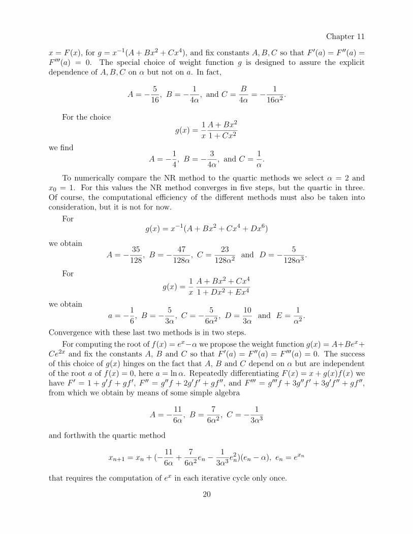
x = F (x), for g = x−1(A + Bx2 + Cx4), and fix constants A,B,C so that F ′(a) = F ′′(a) =F ′′′(a) = 0. The special choice of weight function g is designed to assure the explicitdependence of A,B,C on α but not on a. In fact,

A = − 5

16, B = − 1

4α, and C =

B

4α= − 1

16α2.

For the choice

g(x) =1

x

A + Bx2

1 + Cx2

we find

A = −1

4, B = − 3

4α, and C =

1

α.

To numerically compare the NR method to the quartic methods we select α = 2 andx0 = 1. For this values the NR method converges in five steps, but the quartic in three.Of course, the computational efficiency of the different methods must also be taken intoconsideration, but it is not for now.

Forg(x) = x−1(A + Bx2 + Cx4 + Dx6)

we obtain

A = − 35

128, B = − 47

128α, C =

23

128α2and D = − 5

128α3.

For

g(x) =1

x

A + Bx2 + Cx4

1 + Dx2 + Ex4

we obtain

a = −1

6, B = − 5

3α, C = − 5

6α2, D =

10

3αand E =

1

α2.

Convergence with these last two methods is in two steps.

For computing the root of f(x) = ex−α we propose the weight function g(x) = A+Bex+Ce2x and fix the constants A, B and C so that F ′(a) = F ′′(a) = F ′′′(a) = 0. The successof this choice of g(x) hinges on the fact that A, B and C depend on α but are independentof the root a of f(x) = 0, here a = lnα. Repeatedly differentiating F (x) = x + g(x)f(x) wehave F ′ = 1 + g′f + gf ′, F ′′ = g′′f + 2g′f ′ + gf ′′, and F ′′′ = g′′′f + 3g′′f ′ + 3g′f ′′ + gf ′′,from which we obtain by means of some simple algebra

A = − 11

6α, B =

7

6α2, C = − 1

3α3

and forthwith the quartic method

xn+1 = xn + (− 11

6α+

7

6α2en − 1

3α3e2n)(en − α), en = exn

that requires the computation of ex in each iterative cycle only once.

20

Chapter 11

For the rational

xn+1 = xn +A + Ben1 + Cen

(en − α), en = exn

we have

A = − 5

2α, B = − 1

2α2, C =

2

α.

To find the root of f(x) = lnx− α we propose

xn+1 = xn + xn(A + B lnxn + C ln2 xn)(lnxn − α)

but decide to take C = 0 and find A = −1−α/2, B = 1/2. Halley’s method applied to thisfunction yields the recursion

xn+1 = xn − 2xn2 − α + ln

(ln − α), ln = lnxn.

Correspondingly, we propose

xn+1 = xn + xnA + Bln1 + Cln

(ln − α), ln = lnxn

and find

A =6 + α

−6 + 2α, B =

1

6 − 2α, C =

1

3 − α.

To numerically compare the two methods we choose α = 0.5, so that a =√e, and take

as starting value x0 = 1. Once more, Halley’s method converged in three steps and ourrational method converged in two steps.

Once a good program is available for the evaluation of sinx and cosx, 0 < x < π/2, theinverse trigonometric function arcsinx can be obtained as the solution of sinx− α = 0. Fora cubic iterative solution method we propose to take g(x) = A + B cosx, and we ascertainthat F (a) = F ′′(a) = 0 if A = (3α2 − 2)/(2β3) and B = −α/(2β3), where β =

√1 − α2.

To have a quartic method we suggest g(x) = (A + B cosx)/(1 + C cosx) and ascertain thatF (a) = F ′′(a) = F ′′′(a) = 0 if

A =β

1 + 2α2− 2

β, B =

1

1 + 2α2, C =

−2β

1 + 2α2+

1

β, where β =

√1 − α2.

Halley’s method is here

xn+1 = xn − 2cnc2n − αsn

(sn − α) where cn = cosxn, and sn = sinxn.

We numerically compare the two methods by choosing α = 0.5, so that a = arcsin(0.5) =π/6, and taking as starting value x0 = 1. Using high precision computation to suppress theill effect of arithmetical round-off, we have Halley’s method converge in four steps, and ourrational method in only two.

21