implied volatility and the risk-free rate of return in ...smaclachlan/research/implied.pdf · 1...
TRANSCRIPT

1
Implied Volatility and the Risk-Free
Rate of Return in Options Markets
Marcelo Bianconi* Scott MacLachlan** Marco Sammon*** Department of Economics Department of Mathematics Federal Reserve Bank of Boston Tufts University Tufts University
Abstract This paper implements an algorithm that can be used to solve systems of Black-Scholes equations for implied volatility and implied risk-free rate of return. After using a seemingly unrelated regressions (SUR) model to obtain point estimates for implied volatility and implied risk-free rate, the options are re-priced using these parameters in the Black-Scholes formula. Given this re-pricing, we find that the difference between the market and model priceis increasing in moneyness, and decreasing in time to expiration and the size of the bid ask spread. We ask whether the new information gained by the simultaneous solution is useful. We find that after using the SUR model, and re-pricing the options, the varying risk-free rate model yields Black-Scholes prices closer to market prices than the fixed risk-free rate model. We also find that the varying risk-free rate model is better for predicting future evolutions in model-free implied volatility as measured by the VIX. Finally, we discuss potential trading strategies based both on the model-based Black-Scholes prices and on VIX predictability. Keywords: re-pricing options, forecasting volatility, seemingly unrelated regression, implied volatility JEL Classification Codes: G13, C63
Preliminary Draft, January 2014
Comments Welcome ___________________________________________________________________________________________
*Bianconi: Associate Professor of Economics, [email protected]
**MacLachlan: Associate Professor of Mathematics, [email protected]
***Sammon: Federal Reserve Bank of Boston, [email protected]
____________________________________________
This research is based on Sammon’s thesis at Tufts University, winner of the Linda Datcher-Loury award. We thank the
Tufts Department of Economics for funding the research data and Tufts University for use of the High-Performance
Computing Research Cluster. Any errors are our own.
***Sammon’s views expressed herein are his own and not necessarily of the Federal Reserve Bank of Boston or the
Federal Reserve System.

2
I. Introduction
There are investment firms that pay people to sit outside of factories with binoculars, and count the
number of trucks going in and out. Investors do this because each truck contains information, and
they believe having this information before anyone else gives them an advantage in financial markets.
Every day, several thousands of options are traded, and each trade contains information. In the same
way that information can be gained by watching trucks, there must be a way to capture information by
observing the options market. This paper develops a variant of a model to do just that.
Ever since Black and Scholes (1973), both academics and finance practitioners have used it to
garner information from the options market. One way of doing this is to calculate the implied
volatility of an underlying security, given the market prices of options. Option-implied stock market
volatility even became a tradable asset when the Chicago Board Options Exchange launched the
CBOE Market Volatility Index (VIX) in 1993. Becker, Clements, and White (2007), among others,
study whether or not the S&P 500 implied volatility index (VIX) contains information relevant to
future volatility beyond that available from model based volatility forecasts and find that the VIX
index does not contain any such additional information relevant for forecasting volatility; see also
Canina and Figlewski (1993) and Christensen and Prabhala (1998). Alternatively, Hentschel (2003)
shows that estimating implied volatility by inverting the Black-Scholes formula is subject to
considerable error when option characteristics are observed with plausible errors.1
When calculating implied volatility, however, one must choose a fixed risk-free rate, usually
the yield on Treasury bills. This assumes that Treasury bill yields capture the risk-free rate implicitly
used by market participants buying and selling options. This might not be true for a number of reasons,
including that people buying and selling Treasury bills might have different time preferences than
those trading options and that Treasury bill yields might be heavily influenced by Federal Reserve
asset purchasing programs, and as a result may not reflect market forces. Relaxing this assumption
complicates the interpretation of implied volatility, as it would then contain information on investor
expectations for both the discount rate and the underlying security’s volatility. The assumption isn’t
needed if one sets up a system of two Black-Scholes equations in two unknowns, and solves
simultaneously for the implied volatility and implied risk-free rate. We believe this implied risk-free
1 Also, Jiang and Tian (2005) show that model-free implied volatility is a more efficient forecast of future realized volatility relative to the model based implied volatility.

3
rate might contain valuable information complementary to the usual implied volatility of the
underlying asset.2
Even though the goal is to have a single point estimate of implied volatility and implied
risk-free rate for each underlying security, empirically these values differ among options on the same
security with different strike prices. We build on the methods of Macbeth and Merville (1979) and
Krausz (1985), but suggest using a seemingly unrelated regressions (SUR) model to calculate a point
estimate of at-the-money implied volatility and implied risk-free rate for each underlying security.
These point estimates can be used to re-price the options using the Black-Scholes formula. We
examine the relationship between moneyness, time to expiration and size of the bid-ask spread on the
difference between market prices and model-based Black-Scholes prices.
When running a regression of the difference between market and model prices on the option
characteristics described above, the coefficient on moneyness can be positive or negative across
different regression specifications. The ‘no restrictions’ specification shows that as moneyness
decreases, the model-based Black-Scholes price is likely to greatly exceed the market price. Also, as
an option gets far into the money, the market price is more likely to exceed the model price. Intuitively,
this is explained by the volatility skew. Out of the money options have higher implied volatility, and
as a result have higher model prices.
We find that the size of the bid ask spread and the quality of our solutions measured by an
appropriate extremum move in the same direction indicating lack of liquidity and/or mispricing at
either end of the spread. There are other statistically significant relationships, but the coefficients are
economically small. Alternatively, moneyness and quality move in opposite direction which implies
that very in the money options are easier to price.
The model outlined above, by construction, extracts additional information from the options
market, the key interesting question is whether or not this new information is useful. We provide a
diagnostic of the marginal impact of allowing the risk-free rate to vary in terms of the volatility smile
and the accuracy of market volatility prediction. The difference between the implied volatility
calculated using a fixed r, and the same quantity calculated with r allowed to vary increases over the
sampled period indicating that additional information becomes more important as the sample period
2 Basically, we use the implied risk-free rate for re-pricing options and expect this to be more accurate than using the usual Treasury bill rate.

4
progresses and their correlation is positive across all leads and lags. In addition, the difference
between the market price and the model-based Black-Scholes price shows that the varying risk-free
rate model better fits the data, and potentially provides better estimates of implied volatility.
A possible explanation for why the volatility smile looks different when using the
simultaneous solution method is that there is a balancing effect between the risk-free rate and the
implied volatility. As can be seen in Figure 9, there is a pattern for the implied risk-free rate across
strikes that seems to be the inverse of the pattern for implied volatility. This balancing, however, is not
enough to get rid of the volatility smile, so the problem remains unresolved. For the purposes of
forecasting the VIX, the simple implied volatility model is inferior relative to the joint implied
volatility and implied risk-free rate proposed by our algorithm.
Finally, we outline and examine potential trading strategies based on the discrepancy between
Black-Scholes prices and model prices, and alternatively based on the predictability of the VIX using
model-based prices. The simultaneous and fixed risk-free rate algorithms yield alternative relative
performances in the sample period.
The paper is organized as follows. Section II discusses the simultaneous solution for implied
volatility and the implied risk-free rate. Section III goes over the at-the-money adjustment using the
seemingly unrelated regressions model. Section IV discusses the data used in this paper, and some
descriptive statistics of the results. Section V examines factors that might explain the difference
between the model prices and the market prices. Section VI investigates the marginal effect of
allowing the risk-free rate to vary in several finance problems, while Section VII overviews potential
trading strategies and Section VIII concludes. An appendix presents the mathematical background of
our main algorithm, performance and sensitivity analysis.
II. Simultaneous Solution for Implied Volatility and Implied Risk-Free Rate
This section begins with a brief review of the Black-Scholes formula followed by a brief review of the
literature on simultaneous solutions for implied volatility and implied risk-free rate. We then provide
a description of the algorithm implemented in this paper for finding the simultaneous solution.
II.1. Black-Scholes Formula and Implied Volatility
Black and Scholes (1973) created the following model for pricing a European call option:
Φ Φ (1)

5
where
√√ , S is the spot price of the underlying security, Φ is the normal
CDF, K is the strike price, r is the risk-free rate of return, is the volatility of the underlying asset
and is option’s time to expiration.
For any call traded on an exchange, S, K and are known, but and r, which are meant to be
forward looking, cannot be observed directly. To resolve this issue, finance practitioners applying
Black-Scholes to price options might use the annualized yield on Treasury bills to approximate the
risk free rate, and use historical volatility to approximate future volatility.
It is possible, however, to find the option-implied volatility for the underlying asset if the
option’s market price is known. After deciding on an appropriate value for r, it now becomes a case of
one equation in one unknown. Owing to the fact that it does not enter the Black-Scholes formula
linearly, an optimization routine is needed to solve for implied volatility. If one were using an
algorithm like Newton’s Method, the goal would be to minimize the quadratic function ∗
given , , and from market data and r from Treasury bill yields, where ∗ is the market
price for the call and is the Black-Scholes formula evaluated at . Solving for is useful, as it
captures investor sentiment about the volatility of the underlying asset, but we believe it still leaves
out important information.
As mentioned above, the true risk-free rate is not observable in the market, so it would be
better if both and could be extracted from options data. This is important, because it would
eliminate the need to approximate the risk-free rate with the Treasury bill yields, as these may not
accurately capture option traders’ expectations of changes in the discount rate. The following sections
discuss methods for finding both and .
II.2. Simultaneous Solutions for Implied Volatility and Implied Risk-Free Rate
One can solve for the implied volatility and implied risk-free rate if one can observe two call options,
on the same underlying security with the same time to expiration but different strike prices. This will
yield a system of two equations and two unknowns, which can be solved simultaneously for the
parameters of interest. Authors such as O'Brien and Kennedy (1982), Krausz (1985) and Swilder
(1986) used various methods to find simultaneous solutions for and . This paper builds on their
models, using modern mathematics and statistics software packages which allow for the use of much
larger datasets and more precision in the estimates for and r. Appendix A discusses why an

6
optimization routine is needed to find this simultaneous solution.
The general goal of a simultaneous solution is to solve both , ∗ and ,
∗ where, ∗ and ∗ are the calls’ market prices and , and , are the first and
second calls priced with the Black-Scholes formula evaluated at and . Given that and both
enter non-linearly into the Black-Scholes formula, these parameters cannot be solved for directly.
Krausz’s algorithm picks a starting point, and adjusts and by small increments, and ,
until a solution to the system is found.
To determine how much and should be perturbed, Krausz’s algorithm solves the
following system for and :
, ∗and , ∗ (2)
To simplify the problem, Krausz uses the following first order Taylor approximation, valid for small
and : 3
, , , , (3)
Given the Taylor approximation, Equation (2) can be rewritten in matrix form and solved for and
as follows:
∗ ,∗ ,
(4)
If there is a solution to this system, and are added to and . This process of finding
and and adding them to and is repeated until the assumptions of the Black-Scholes model
are violated. For example, the addition of and would make or r less than zero) or until
and become sufficiently small where Krausz stopped when and were smaller than 10 .
This method, however, is slow, as it requires taking four derivatives of the Black-Scholes formula at
each step. In addition, this method may not always find a solution as it relies on the assumption that a
solution to , ∗ and , ∗ exists, which may not be the case for real-world (noisy)
data.
II.3. Proposed Method for Finding a Simultaneous Solution
Rather than set up two equations in two unknowns, we propose a single equation to be minimized for
3 Krausz (1985) limited the size of and when adjusting and in each iteration. In Equation 4, after solving for these quantities he would multiply them by some constant so they would not exceed a maximum size and the Taylor approximation would still be sufficiently accurate.

7
and r with an optimization routine:
, ∗∗ , ∗
∗ , (5)
This equation has advantages over the two equations model discussed above, in that it has a
mechanism for weighing the difference between the Black-Scholes price and the market price. This is
important, because if the second option in the pair were much more expensive, the solution for and
r would be biased toward minimizing ∗ , using Krausz’s method. In addition, minimizing
this function does not rely on the assumption that an exact solution exists such that , 0,
which means it has a much lower failure rate of finding solutions. The function F can be interpreted as
a measure of the quality of our solutions and will be sensitive to moneyness, bid-ask spread and time
to expiry according to our projections below.
A number of different algorithms in MATLAB were tested for minimizing this equation, and
while the main body of the paper focuses on algorithms built into the fmincon function, alternative
optimization models are discussed in Appendix B. Within the fmincon function, we experimented
with two algorithms: sequential quadratic programming (SQP) and interior point. In both cases, the
algorithms actually ran slower when we provided gradient and Hessian information, so we used
derivative-free approaches. These methods approximate the gradient using finite differences, and use
the Broyden-Fletcher-Goldfarb-Shanno (BFGS) method to approximate the Hessian. Both SQP and
interior point use similar approaches at each step of the optimization, but they implement range
constraints, restricting both and to be in the range of 0 to 1, differently
The interior point algorithm tries to find a location where the gradient is equal to zero, but it
weighs the quality of solutions by how close they are to the range constraints. We decided to impose
the restriction that and must be between zero and one, because values outside of this range seem
empirically unrealistic. When looking for a minimum, this algorithm will continue to choose points
that are opposite the direction of the gradient (downhill) until it reaches a balance between getting the
gradient close to zero, and staying far enough from the edge of the feasible set.
The SQP algorithm takes a second-order Taylor Series approximation of the function to be
minimized. Such a quadratic approximation can be directly minimized, similarly to the linearizations
used in Newton's method, allowing iterative improvement of the approximate minimization of the
non-linear (and non-quadratic) function F. Unlike interior point, this algorithm does not discount the

8
quality of solutions where and are close to the edge of the feasible set. The algorithm continues
to take these Taylor Series approximations, and adjust and , until the gradient of F is sufficiently
near zero.
Although interior point requires more calculations than SQP per iteration, this was not an issue
when minimizing , as it ended up being faster on average than SQP. In addition, interior point
achieved more accurate solutions, with smaller average values of . 4 It is also important to note that
both of these algorithms were faster and more accurate than the algorithm developed by Krausz
(1985). This algorithm is faster than two simple alternatives: a brute-force approach that directly
samples , on an evenly space mesh of 200 values of each of and (sampling 40,000 total
points); and an algorithm that applies a classical Newton's method to directly minimizing F by
satisfying its first-order optimality conditions.
The final algorithm used for this paper is as follows:
1. The starting values of and for each pair of options is (0.5, ) where is the Treasury bill
yield on the data’s date.
2. The interior point algorithm is used to find a simultaneous solution for and , starting at the
point determined in step 1.
3. The patternsearch algorithm (another derivative-free method in MATLAB’s optimization toolbox)
is run to minimize F, starting from the point found in step 2, to find another possible solution and
.
4. Starting at the point found in step 3, the interior point algorithm is run again to minimize F, and find
a third possible solution for and .
5. The algorithm accesses the three values of F from steps 2, 3 and 4, choosing the ( , ) pair which
yields the smallest F.
III. At-the-Money Adjustment
After running the algorithm discussed in Section II, we obtain an implied volatility and implied risk
free rate for each pair of options. In order to proceed with re-pricing the options, we need to find a
point estimate for implied volatility and implied risk free rate for each underlying security. This
4 See appendix B for a comparison of speed and accuracy between these two algorithms.

9
section reviews potential approaches and discusses our version of the at-the-money adjustment, a
method weighing the individual estimates.
When working with a large number of options, each option on the same underlying security
will most likely have a different implied volatility. Given that implied volatility is supposed to be a
measure of volatility for the underlying security, and not the option, an adjustment should be made to
extract a single point estimate for this parameter.
This point estimate should not be calculated using a geometric average, given the presence of
two common phenomena for options, the volatility skew and the volatility smile. The volatility skew
is when implied volatility is highest for out-of-the-money (OTM) options, and decreases steadily as
strike prices increase.5 The volatility smile is when volatility is lowest for at-the-money options, and
it increases as options become deeper in-the-money (ITM) or farther OTM. An example of the
volatility smile from the dataset used in this paper is shown in Figure 1.
Figure 1:
To adjust for the volatility skew and the volatility smile, Macbeth and Merville (1979) ran the
following ordinary least squares (OLS) regression:
(6)
where is the model implied volatility for an option j, on security k, at time t, is the error 5 This section only discusses strike skew, where implied volatility is different across options on the same underlying security with the same time to expiration. The other type of skew is time skew, where options on the same underlying security with the same strike price have different implied volatilities for each time to expiration.
.51
1.5
2Im
plie
d V
olat
ility
100 150 200 250Strike Price
Note: All of these options are two weeks from expiration
Data from December 10, 2007Implied Volatility on AAPL Options

10
term and is a measure of moneyness, is the price of the underlying security,
is the present value of the option’s strike price and r is the Treasury bill interest rate. The
term equals zero when, on a present value basis, an option is at-the-money, so the estimate
is the implied at-the-money volatility. Essentially, is a weighted average of all the different
implied volatilities calculated for options on a particular security, where the weight is determined by
moneyness. Krausz (1985) adapts this technique to his simultaneous solution for and . He runs an
OLS regression to adjust each parameter:
(7)
and
(8)
where and are the model implied values for implied-volatility and risk-free rate for an
option, j on security, k at time, t. In addition, ∗
∗ where is the price of the
underlying security, ∗
is the present value of the option’s strike price, and ∗ is the average
model implied risk-free rate across all securities on a given date. In this model, and are
error terms. The at-the-money implied volatility and risk free rate for each security are and
. As in the Macbeth and Merville (1979) model, 0 when, on a net present value basis, an
option is at the money.
III.1. Proposed At-the-Money Adjustment
Using the average value of r in the calculation of , ∗, causes an endogeneity problem, in that
will be on both sides of Equation (8). In addition, the fact that these regressions are run separately
omits the simultaneity of the solution for and . It is possible, however, to account for this by
rewriting in a way that isolates r. First, we move all terms that contain r to the left hand side of
the equation:
→ 1 (9)
Then, we take the natural log of each side and solve for :
ln 1 ln ln ln . (10)
For 0, we have thatln 1 , so we can approximate (10) as

11
ln ln . (11)
Substituting this into Krausz’s Equations (7) and (8) gives
ln ln (12)
and
ln ln . (13)
An additional adjustment is required because is still on both sides of the second equation.
The second equation can be solved explicitly for as follows
ln ln ′ . (14)
As with the Macbeth and Merville (1979) model, the constant terms, and
represent the at-the-money implied volatility and risk-free rate for the underlying security because
ln ln 0 for options expiring at the money.
The following steps outline our method for explicitly identifying . In order to find ,
we start by taking a linear approximation of for < 1 which given the units is safe to
assume. We can rewrite as the geometric series 1 + ⋯ . While a higher
order approximation would give more accurate results, this must be weighed against the additional
computational cost. A first order approximation was used so that
1 1 ′′ (15)
which can be simplified as follows:
′′ 6 (16)
In this equation, , is the model-implied risk-free rate and .
Another improvement in the at-the-money adjustment developed in this paper is that it
accounts for the simultaneity of and , in that it uses a seemingly unrelated regressions (SUR)
model for the two equations. The assumption of a SUR model is that the error terms across the
regressions are related, which makes sense given every and is extracted from a single pair of
options on the same underlying asset with the same time to expiration. 6 The number of iterations allowed in the SUR model for the variance-covariance matrix to converge was limited to 1,000.

12
The implications of using the SUR model are more evident when one considers shocks
entering the system. Without using SUR, a shock in the error term for the risk-free rate regression has
no impact on the volatility regression. With SUR, a shock in the error term for the risk-free rate
regression will also cause a shock in the error term for implied volatility regression, and vice versa.
Bliss and Panigirtzoglou (2004) explain that, “risk preferences are volatility dependent”. Given the
close relationship between implied risk-free rate and the implied volatility, it makes sense that a shock
affecting one of these equations should also affect the other. Finally, is that if there is correlation
between the error terms in the two equations, using the SUR will yield smaller standard errors for the
estimated coefficients.7
IV. Data
IV.1. Data Sources and Description
The options dataset used for all empirical analysis in this paper is from
http://www.historicaloptiondata.com/, and it contains end of day quotes on all stock options for the
U.S. equities market. This includes all stocks, indices and ETFs for each strike price and time to
expiration. Data on the VIX, Treasury bills and other market indices was collected from the Federal
Reserve Bank of St. Louis. The empirical work in this paper focuses on data from March 2007-March
2008. Given that we are interested in implied volatility and the risk-free rate, Figure 2 shows the
evolution of these two quantities, as measured by the VIX8 and 3-month Treasury bills, over the
period of interest. It can be seen that the risk free rate is trending downward, while the implied
volatility is increasing.
7 SUR will only make the standard error smaller if two conditions are met: (1) There is correlation between the standard errors in the regressions (2) the two equations have different independent variables. For example: running the two regressions and as OLS regressions will be no different than running them as SUR regressions because they both only have on the right hand side. In our model, the right hand side is slightly different for each equation, and we have good reason to believe the standard errors will be correlated, so there should be efficiency gains. 8 The new VIX is a model free calculation of volatility based upon the prices of S&P500 index options and it does not rely on the Black-Scholes framework. See e.g. CBOE (2009).

13
Figure 2:
VI.2. Restrictions on the Data
A subset of the data was chosen for analysis in this paper using a procedure similar to that of
Constantinides, Jackwerth and Savov (2012). First, the interest rate implied by put-call parity was
computed. The equation for put-call parity can be solved algebraically for as follows:
(17)
All the observations with values of that did not exist or were less than zero were
dropped. Constantinides et al. (2012) removed these options because these values for
suggest that the options are probably mispriced. After this calculation, all of the puts were removed
from the dataset, as this paper only focuses on call options. Other procedures in line with
Constantinides et al. were the removal of options with bid prices of zero and options with zero open
interest. Options with zero volume for a given day, however, were allowed to remain in the dataset9.
IV.3. Descriptive Statistics
Figure 3 shows the evolution of the daily average of option-implied risk-free rate and volatility for
SPX options, cash-settled options on the S&P 500 index, and how this compares to movements in
benchmarks for these two quantities.10 It can be seen that changes in the average option-implied
9 Open interest is the total number of option contracts that have been traded, but not yet liquidated. Volume is
measured in shares, and is only useful as a relative measure; it should be compared to average daily volume for
underlying security, rather than across securities.
10 There are two commonly traded S&P 500 index options, SPX and SPY. SPX options are based on the entire
10
15
20
25
30
35
VIX
Perc
enta
ge P
oin
ts
.01
.02
.03
.04
.05
Tre
asu
ry B
ill R
ate
01ap
r200
7
01jul200
7
01oc
t200
7
01jan2
008
01ap
r200
8
Annualized 3-Month Treasury Bill Rate VIX
Implied Volatility and the Risk-Free Rate

14
risk-free rate do not seem to be related to changes in Treasury bill rate. In addition, the option-implied
volatility seems detached from the VIX index. It should be noted that these averages for implied
volatility and implied risk-free rate are calculated for values when these parameters are between zero
and one, because as discussed above, values outside of this range seem economically unrealistic. A
possible interpretation of the lack of relationship between the series calculated in this paper, and the
benchmark series is that the old assumptions about Treasury bills representing the risk-free rate were
false, and we are indeed getting new information through the simultaneous solution.
Figure 3:
In Figure 4, we compare the implied volatility, calculated with the risk-free rate fixed at the
3-month Treasury bill rate, to the VIX index. Unlike the line graphs above, these two series seem to
generally follow the same trend. This is not surprising because according to the CBOE website: “The
basket of underlying securities, and are settled in cash while the SPY is based on an ETF, settled in shares. All these averages are based on the values before the at-the-money adjustment.
0.0
5.1
.15
.2
01ap
r200
7
01jul
2007
01oc
t200
7
01jan
2008
01ap
r200
8
Option Implied Risk-Free Rate 3-Month T-Bill Rate
Risk-Free Rate Comparison
10
15
20
25
30
35
VIX
Pe
rcen
tage
Po
ints
.12
.14
.16
.18
.2.2
2O
ptio
n-Im
plie
d V
olat
ility
01ap
r200
7
01jul
2007
01oc
t200
7
01jan
2008
01ap
r200
8
Option Implied Volatility VIX
Volatility Comparison

15
risk-free interest rate, R, is the bond-equivalent yield of the U.S. T-bill maturing closest to the
expiration dates of relevant SPX options.” Both of these calculations use the same fixed risk free rate.
Figure 4:
A possible explanation for why the relationship between the VIX and option-implied volatility
seems weaker when using the simultaneous solution is that our model better isolates investor
expectations about volatility than the VIX.
Table 1 below presents some descriptive statistics across all days in the sample period. We
experimented with several different restrictions on the data as follows. We define
′ (18)
and the restriction on ′ is within one standard deviation of its mean (which excludes very far in the
money and out of the money options). The restriction on time to expiration is to options expiring more
than 90 days in the future. It should also be noted that these averages are restricted to observations
where the variables of interest are between zero and one.11
In almost all cases, making these restrictions does not make a significant difference in the
variables’ averages. This is important, because it shows that the conditional mean of each variable
based on some factors like moneyness is almost the same as the unconditional mean. The one case
where it does make a significant difference is the time to expiration restriction on the average risk-free
rate before the at the money adjustment. This implies that options closer to expiration have a higher
11 We make those restrictions because it is well known that far out-of-the-money options are poorly priced by Black-Scholes, and that option prices become more volatile as time to expiration gets smaller.
10
15
20
25
30
35
VIX
Perc
enta
ge P
oin
ts
.05
.1.1
5.2
.25
.3O
ptio
n-Im
plie
d V
olat
ility
01ap
r200
7
01jul200
7
01oc
t200
7
01jan2
008
01ap
r200
8
Option-Implied Volatility VIX
Implied Volatility (fixed risk-free rate) and the VIX

16
option-implied risk free rate. If this risk free rate captures investor expectations as we proposed above,
this could signal that there was much more short-term uncertainty at the time than long term
uncertainty, which is why the short-term implicit discount rate was so high.
Table 1: Descriptive Statistics under Alternative Restrictions
_____________________________________________________________________
V. Determinants of Underpricing/Overpricing
This section presents a summary of the results from the applied algorithm and the analysis of the
regressions on factors that determine the difference between model-based Black-Scholes prices and
market prices.
V.1. Macbeth and Merville Regressions
Macbeth and Merville (1979) solved for implied volatility and after making the at-the-money
adjustment, they re-priced the options using the new value for this parameter.12 They then wanted to
examine possible determinants of differences between market prices and Black-Scholes prices. Their
dependent variable was:
, (19)
and their independent variables were moneyness and time to expiration. We propose a similar model,
with our regression:
′ (20)
where is the difference between the market price and the Black-Scholes model price for an
12 Macbeth and Merville (1979) did not use a simultaneous solution to find the implied risk-free rate.
No Restrictions Restrict M'
Restrict Time to
Expiration Restrict F
Average Risk‐Free
Rate 0.0932 0.0944 0.0883 0.0946
Average ATM Risk‐
Free Rate 0.1237 0.1214 0.1218 0.1228
Average Implied
Volatility 0.3536 0.3365 0.3437 0.3509
Average ATM
Implied Volatility 0.3767 0.3645 0.3797 0.3735

17
option i, on security k, at time t, ′ , is the annualized coupon equivalent on a
13-week Treasury Bill, is the time to expiration, , and is
an error term.
Table 2 below presents the averages across all dates for key variables across different
specifications. The restrictions on moneyness, time to expiration and F are the same as those
described in Section IV.
Table 2: Descriptive Statistics under Alternative Restrictions cont.
_____________________________________________________________________
Table 3 below presents the regression results. Across different specifications, the coefficient
on moneyness can be positive or negative. This could imply that there are very far in the money and
out of the money options that are biasing the regression results, given that the coefficient is only
negative in the regression where moneyness itself is restricted. Based on the ‘no restrictions’
specification, as an option goes very far out of the money (moneyness decreases) the Black-Scholes
price is likely to greatly exceed the market price. Also, as an option gets far into the money, the
market price is more likely to exceed the model price. This relationship, however, is reversed when
moneyness is within one standard deviation of the mean, as the coefficient on moneyness is negative
and significant in the restricted moneyness specification.13
13 We also tried using percentage differences 100as the dependent variable, but this function
does not exist for a large number of options with either market prices, or Black-Scholes prices close to zero.
No Restrictions Restrict M'
Restrict Time to
Expiration Restrict F
Moneyness 0.2117 0.1112 0.2407 0.2288
Time to Expiration 0.6161 0.5606 0.8442 0.6271
Spread ‐0.1792 ‐0.1742 ‐0.1709 ‐0.1626
F 0.0072 0.0066 0.0039 0.0002
Y ‐1.8065 ‐1.7799 ‐2.4808 ‐1.8758
# Obs 15,700,000 13,600,000 10,800,000 15,000,000

18
Table 3: Regressions Estimated model is ′ ,
where is the difference between the market price and the Black-Scholes model price for an option i, on
security k, at time t, ′ , is the annualized coupon equivalent on a 13-week Treasury
Bill, is the time to expiration, , and is an error term.
_____________________________________________________________________
_____________________________________________________________________
* 10% level, ** 5% level, ***1% level
V.2. Others Explanations for the Differences between Model Prices and Market Prices
A limitation of the research presented in this paper is that we did not adjust for dividends, even though
many of the underlying securities in the dataset used for the empirical portion of this paper are
dividend paying. Merton (1973) presented an adjustment to the Black-Scholes formula for stocks that
pay dividends. Owing to the fact that the option price is decreasing in dividend yield, this will make
the average Y in this paper generally smaller in absolute value than it should be if an adjustment for
dividends were made, owing to the fact that the model price on average always exceeds the market
price (see Figure 10).
In addition to the dividend issue mentioned above, we want to see if there are certain types of
options which are more likely to have low quality solutions, as measured by the size of F. We ran the
following regression for several specifications:
′ (21)
and the results are presented in Table 4. It is not surprising that in every specification, as the size of the
bid ask spread gets larger, so does F, as this indicates illiquidity and/or mispricing at either end of the
spread. There are other statistically significant relationships, but the coefficients are economically
small. As moneyness increases F decreases, which implies that very in the money options are easier to
No Restrictions Restrict M'
Restrict Time to
Expiration Restrict F
Moneyness 0.392*** ‐0.409*** 0.572*** 0.457***
Time to Expiration ‐3.091*** ‐3.265*** ‐3.222*** ‐3.149***
Spread ‐2.199*** ‐1.723*** ‐3.458*** ‐2.472***
Constant ‐0.379*** ‐0.203*** ‐0.484*** ‐0.409***
# Obs 16,016,475 13,847,564 10,824,043 15,016,942

19
price perhaps, because they behave more like a stock than an option, i.e. an option with strike zero
behaves exactly like the stock. The coefficient on time to expiration is insignificant in the regressions
where we don’t restrict this variable, which leads us to believe the effect of time to expiration on F
might be opposite for options close to and far from expiration, which is why when time to expiration
is restricted to greater than 90 days, the relationship becomes significant.
Table 4: Regressions
Estimated model is ′ where is the quality of
solution for an option i, on security k, at time t, ′ , is the annualized coupon equivalent on
a 13-week Treasury Bill, is the time to expiration, , and is an error
term.
_____________________________________________________________________
_____________________________________________________________________
* 10% level, ** 5% level, ***1% level
VI. Marginal Effect of Allowing Risk-Free Interest Rate to Vary
As was mentioned above, finding the simultaneous solution and making the at-the-money adjustment
yields more information. The interesting question is whether or not this additional information is
useful. The following section goes over some comparisons between the new and old information sets,
as well as some applications of this new information.
Figure 5 plots the difference between the implied volatility calculated using a fixed r, and the
same quantity calculated with r allowed to vary. Note that all these plots are just based on data for
SPX options, and they exclude values where the variables of interest are not between zero and one.
The difference increases over the sampled period indicating that additional information becomes
more important as the sample period progresses.
No Restrictions Restrict M'
Restrict Time to
Expiration
Moneyness ‐0.0689*** ‐0.0964*** ‐0.00895***
Time to Expiration ‐0.00775 0.0109 0.00592***
Spread 0.164*** 0.157*** 0.0522***
Constant 0.0521*** 0.0173 ‐0.00257***
Observations 17100528 14675713 11543771

20
Figure 5:
Figure 6 presents the cross correlation function between the implied volatility calculated using
a fixed r, and the same quantity calculated with r allowed to vary. We note that as expected, they are
positively correlated across all leads and lags at about 50%, with a peak at the contemporaneous
correlation over 50%.
Figure 6:
VI.1. Volatility Smile
It is well known that in practice the implied volatility is different across strike prices in the
Black-Scholes model. We wanted to see if allowing the risk-free rate to vary would change the
differences in implied volatility across strikes, i.e. would change the volatility smile. Figure 7 shows
the case for AAPL options. Allowing r to vary did not seem to change the pattern very much, as the
volatility smile still clearly exists.
-.1
-.05
0.0
5.1
.15
01ap
r200
7
01jul200
7
01oc
t200
7
01jan2
008
01ap
r200
8
DifferenceMarginal Impact of Simultaneous Solution
-1.0
0-0
.50
0.0
00.5
01.0
0
-1.0
0-0
.50
0.0
00.5
01.0
0
-20
-10 0 10 20
Cross CorrelationMarginal Impact of Simultaneous Solution

21
Figure 7:
Figure 8 is a similar plot for GOOG options. Although the volatility skew is still apparent in
the graph on the left, the pattern certainly seems less clear defined when r is allowed to vary.
Figure 8:
.3.6
.91.
21.
51.
8Im
plie
d V
olat
ility
100 150 200 250Strike
Varying Risk-Free Rate
.3.6
.91.
21.
51.
8Im
plie
d V
olat
ility
100 150 200 250Strike
Fixed risk-free rate
This data is from Apple options on December 10, 2007 with an expiration date of December 22, 2007The value of Apple stock at close on December 10, 2007 was 194.21
Volatility Smile, Apple Options
.25
.3.3
5.4
.45
.5.5
5Im
plie
d V
olat
ility
200 400 600 800 1000 1200Strike
Varying Risk-Free Rate
.25
.3.3
5.4
.45
.5.5
5Im
plie
d V
olat
ility
200 400 600 800 1000 1200Strike
Fixed risk-free rate
This data is from Google options on January 16, 2008 with an expiration date of January 17, 2009The value of Google stock at close on January 16, 2008 was 615.95
Volatility Skew, Google Options

22
A possible explanation for why the volatility smile looks different when using the
simultaneous solution method is that there is a balancing effect between the risk-free rate and the
implied volatility. As can be seen in Figure 9, there is a pattern for the implied risk-free rate across
strikes that seems to be the inverse of the pattern for implied volatility. This balancing, however, is not
enough to get rid of the volatility smile, so the problem remains unresolved.
Figure 9:
VI.2. Difference between market price and Black-Scholes price
If we look at the evolution of the difference between the market price and the Black-Scholes price, it
can be seen in Figure 10 that the simultaneous solution is generally more accurate than the model with
a fixed risk-free rate controlling in both cases for the at-the-money adjustment and re-pricing the
options. This shows that the varying risk-free rate model better fits the data, and at a minimum
probably provides better estimates of implied volatility.
0.0
5.1
.15
.2R
isk-
Fre
e R
ate
100 150 200 250Strike
Apple Options
0.0
5.1
.15
.2R
isk-
Fre
e R
ate
200 400 600 800 1000 1200Strike
Google Options
These are same options used in the previous two graphics
Risk-Free Rate Frown

23
Figure 10:
VI.3. Predicting Volatility
In order to capture the accuracy of the VIX prediction under alternative risk-free rates assumptions,
we estimate in-sample and out-of-sample forecasts of the VIX on SPX options, because the VIX is
designed to track volatility on the S&P 500 index as measured by the prices of these options. Figure
11 shows the VIX and the at-the-money implied volatilities with varying and fixed risk-free solutions
for data from March 2007 to March 2008.14
Figure 11:
14 The data on option implied volatility represent the average of that variable across all observations on that day, or all cash- settled options on the S&P 500 index.
-15
-10
-50
01ap
r200
7
01jul200
7
01oc
t200
7
01jan2
008
01ap
r200
8
Varying Risk-Free Rate Fixed Risk-Free Rate
Average Difference Between Market and Black-Scholes Price
.1.2
.3.4
.5.6
Impl
ied
Vol
atili
ty
10
15
20
25
30
35
VIX
Index
01apr2007 01jul2007 01oct2007 01jan2008 01apr2008
VIX Index SS ATM Implied Volatility
FRF ATM Implied Volatility
Note: Only data from SPX options
The VIX Index and Option Implied Volatility

24
The univariate econometric models were appropriately obtained via time series identification
as
∑ ∑ (22)
where is the at-the-money implied volatility for the two alternative cases. The
models where estimated via maximum likelihood. The in-sample predictions refer to the forecast
error while the out-of-sample was obtained running the model on the sample March 2007 to
October 2007, and obtaining the out-of-sample dynamic predictions for the remaining periods. In
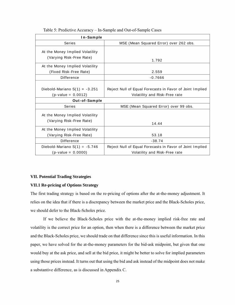
both cases, we use the Diebold and Mariano (1995) test to determine which forecast is more accurate.
The results for the in-sample case are in Table 5, which gives evidence in favor of the joint implied
volatility and implied risk-free rate model. The out-of-sample case, also in Table 5, confirms the
in-sample results. We ran several alternatives including static forecasts and the results are similar and
robust.
For the purposes of forecasting the VIX, the simple implied volatility model is inferior relative
to the joint implied volatility and implied risk-free rate proposed by our algorithm.15
15 The regressions and additional models will be posted on a website with additional materials and are available upon request.
25
Table 5: Predictive Accuracy – In-Sample and Out-of-Sample Cases
In-Sample Series MSE (Mean Squared Error) over 262 obs.
At the Money Implied Volatility (Varying Risk-Free Rate)
1.792 At the Money Implied Volatility
(Fixed Risk-Free Rate) 2.559 Difference -0.7666
Diebold-Mariano S(1) = -3.251
(p-value = 0.0012) Reject Null of Equal Forecasts in Favor of Joint Implied
Volatility and Risk-Free rate Out-of-Sample
Series MSE (Mean Squared Error) over 99 obs.
At the Money Implied Volatility (Varying Risk-Free Rate)
14.44 At the Money Implied Volatility
(Varying Risk-Free Rate) 53.18 Difference -38.74
Diebold-Mariano S(1) = -5.746 (p-value = 0.0000)
Reject Null of Equal Forecasts in Favor of Joint Implied Volatility and Risk-Free rate
VII. Potential Trading Strategies
VII.1 Re-pricing of Options Strategy
The first trading strategy is based on the re-pricing of options after the at-the-money adjustment. It
relies on the idea that if there is a discrepancy between the market price and the Black-Scholes price,
we should defer to the Black-Scholes price.
If we believe the Black-Scholes price with the at-the-money implied risk-free rate and
volatility is the correct price for an option, then when there is a difference between the market price
and the Black-Scholes price, we should trade on that difference since this is useful information. In this
paper, we have solved for the at-the-money parameters for the bid-ask midpoint, but given that one
would buy at the ask price, and sell at the bid price, it might be better to solve for implied parameters
using those prices instead. It turns out that using the bid and ask instead of the midpoint does not make
a substantive difference, as is discussed in Appendix C.

26
We define a simple strategy to use the information from the data.
i. If the market price exceeds the Black-Scholes price, sell/write that call option, and to hedge this
position, buy the underlying security;
ii. If the market price is lower than the Black-Scholes price, buy that call option.
It is possible to hedge this second position of going long on the call by shorting the stock, but for
simplicity we will avoid shorting. In addition, any trading strategy requires transaction costs to
buy/sell the options and underlying security, again, for simplicity, this is ignored in the context of this
example. Also, we calculated the difference on a percentage basis, and dropped all observations for
which the market price and Black-Scholes price differed by more than 20%. Finally, we did not make
any trades for observations where the difference was zero.16
The trading strategy described above was implemented for March 1st 2007 when there were
502 SPX options traded which met the above selection criteria. The return for each option is
calculated and added to the return on the stock if the position was hedged. We then calculate the
average return for the strategy.17 We excluded options expiring on March 21st 2008, because we could
not get a price for the S&P 500 index, and thus could not calculate the exercise value of those options
because the S&P data from Yahoo Finance and from FRED are both missing this day. Under
simultaneous risk-free rate, the average return was about 38%, and the standard deviation was about
39%, both of which seem fairly high. Implementing this same strategy on November 30th, 2007 yields
an average return of about -80%, with a standard deviation of about 29%, suggesting that the average
return is heavily dependent on the day which the strategy is implemented. Also, these returns should
be measured on a risk-adjusted basis. A popular measure for this is the Sharpe ratio:
where is the expected portfolio return, is the risk-free rate of return and is the
standard deviation of portfolio returns. For the March 1st 2007 data, the risk-free rate as measured by
3-month treasury bills was about 5%, making the Sharpe ratio less than one. The standard deviation
would probably be lower if we could hedge the long call positions, as those greatly increase standard
16 Options that differed by more than 20% were largely mispriced (in our opinion), and there was probably an unusual event or a data anomaly that can explain this difference. We also thought about restricting F to be smaller than a specific value, but after dropping all values that differ by more than 20%, almost all observations already have small values of F. We did, however, restrict the strategy to options with 90 or more days to expiration, given options close to expiration can have unusual price fluctuations. 17 We did not weight each position by the degree of mispricing, but that is another possible strategy.

27
deviation when they go to zero expiring out of the money.
The same strategy was implemented, but instead of re-pricing the calls with the at-the-money
implied volatility from the simultaneous solution, it was done with the at-the-money implied
volatility calculated with a fixed risk-free rate. This allows for an evaluation of the marginal impact of
the additional information from a simultaneous solution, by seeing if it leads to a more effective
trading strategy. For the March 1st 2007 data there was an average position return of about 24%, and a
standard deviation of about 7.5%. On a risk-adjusted basis, this yields better returns than the strategy
using the simultaneous solution.
VII.2 VIX Prediction Strategy
Another potential trading strategy is based on predicting the VIX index. It relies on the idea that it is
possible to reliably predict the index, and make trades based on its expected future value. In this case,
we use the econometric model (22) to obtain one-step-ahead forecasts of the VIX index and define a
simple strategy as follows:
i. A position initiated during a given trading day must be closed before the end of that trading day.
Assume positions held overnight do not collect interest.
ii. If the next period predicted VIX is higher than the current level of the VIX, put the entire portfolio
into shares of a product that closely tracks the VIX, and sell them at the end of the next trading day.18
Assume there is no tracking error between these products and the index itself.
iii. If the next period predicted VIX is lower than the current level of the VIX, keep the entire portfolio
in cash for the next trading day.
While it would be possible to hedge the long position for the VIX, this will be avoided for
simplicity. In addition, any trading strategy requires transaction costs to buy/sell the product, and for
simplicity, this is ignored in the context of this example.
We implement the strategy for SPX options. The model described in Equation (22) was
estimated using the first 160 trading days in our sample to calibrate the model. The forecasts after that
were iterative, in that the model was re-estimated for every forecast using all data points before the
one to be predicted. The hypothetical portfolio started with $100,000. A “benchmark” strategy only
includes the two autoregressive terms of the VIX in Equation (22) when forecasting, while the other
strategies include measures of model based at-the-money implied volatility. Figure 12 shows the 18 There are a variety of exchange traded products designed for this including NYSE ARCA: CVOL.

28
value of this hypothetical portfolio over time. This illustrates the main result that the simultaneous
and fixed risk-free rate algorithms yield alternative relative performances in the sample period. In
particular, the simultaneous risk-free interest rate dominates the fixed risk-free interest rate case in the
later periods but the reverse occurs in the earlier periods.
Figure 13:
VIII. Summary and Conclusions
This paper implements an algorithm that can be used to solve systems of Black-Scholes equations for
implied volatility and implied risk-free rate. We use a seemingly unrelated regressions (SUR) model
to calculate a point estimate of at-the-money implied volatility and implied risk-free rate for each
underlying security. These point estimates can be used to re-price the options using the Black-Scholes
formula. We examine the impact of moneyness, time to expiration and size of the bid-ask spread on
the difference between market prices and model-based Black-Scholes prices.
We find that across different specifications, the effect of moneyness on prices can be positive
or negative. The ‘no restrictions’ specification shows that as moneyness decreases, the model-based
Black-Scholes price is likely to greatly exceed the market price. Also, as an option gets far into the
money, the market price is more likely to exceed the model price. The size of the bid ask spread and
the quality of our solutions move in the same direction indicating lack of liquidity and/or mispricing
100
000
150
000
200
000
250
000
Po
rtfo
lio V
alu
e
160 180 200 220 240 260Trading Days Since from March 1, 2007
Simultaneous R Fixed R
Benchmark
Note: All of these strategies are based on one-step-ahead forecasts of the VIX with AR2 terms
VIX Strategy

29
at either end of the spread. Alternatively, moneyness and quality move in opposite direction which
implies that very in the money options are easier to price.
We provide a diagnostic of the marginal impact of allowing the risk-free rate to vary in terms
of the volatility smile and the accuracy of market volatility prediction. The difference between the
implied volatility calculated using a fixed r, and the same quantity calculated with r allowed to vary
increases over the sampled period indicating that additional information becomes more important as
the sample period progresses and their correlation is positive across all leads and lags. The difference
between the market price and the model-based Black-Scholes price shows that the varying risk-free
rate model better fits the data, and potentially provides better estimates of implied volatility. For the
purposes of forecasting the VIX, the simple implied volatility model is inferior relative to the joint
implied volatility and implied risk-free rate proposed by our algorithm.
Finally, we outline two potential trading strategies based on our analysis. One uses the
discrepancy between Black-Scholes prices and model prices, and compares this strategy’s
risk-adjusted return to a similar strategy setting a fixed risk-free rate. The other is based on predicting
the VIX index. In both cases, the simultaneous and fixed risk-free rate algorithms yield alternative
relative performances in the sample period.
There are several avenues for future research that seem to us fruitful. A key one would be to
expand on the computational capability and improve the accuracy of the algorithm using more
nonlinear terms in the model-based prices. Expanding the sample period to more recent years and a
more systematic information index of the gains from implied risk-free rates on implied volatility
could potentially be used in parallel to the VIX as a measure of market volatility. In general, we
believe options prices present important information content of future expectations that can provide
essential for market participants and policy makers.

30
References Becker, R., Clements, A. C., White, S., 2007, Does implied volatility provide any information beyond
that captured in model-based volatility forecasts? Journal of Banking and Finance 31, 2535–2549.
Black, Fischer, and Myron Scholes. "The Pricing of Options and Corporate Liabilities." Journal of
Political Economy 81.3 (1973): 637. Print. Black, Fischer. "Fact and Fantasy in the Use Of Options." Financial Analysts Journal 31.4 (1975):
36-41. Print. Black, Fischer. "How To Use The Holes In Black-Scholes." Journal of Applied Corporate Finance
1.4 (1989): 67-73. Print. Bliss, Robert R., and Nikolaos Panigirtzoglou. "Option-Implied Risk Aversion Estimates." The
Journal of Finance 59.1 (2004): 407-46. Print. Canina, L., Figlewski, S., 1993, The informational content of implied volatility, Review of Financial
Studies 6, 659–681. CBOE Volatility Index - VIX (2009) Chicago Board Options Exchange, Incorporated. Christensen, B. J., Prabhala, N. R., 1998, The relation between implied and realized volatility,
Journal of Financial Economics 50, 125–150. Constantinides, George, Jens Carsten Jackwerth, and Savov Savov. "The Puzzle of Index Option
Returns." (2012), The University of Chicago, Booth School, working paper. n. pag. 9 Feb. 2012. Web.
Diebold, Francis and Roberto Mariano, "Comparing Predictive Accuracy," Journal of Business and
Economic Statistics, 13:3, (1995), 253-263. Hentschel, L., 2003, Errors in implied volatility estimation, Journal of Financial and Quantitative
Analysis 38, 779–810. Jiang, G., Tian, Y., 2005, Model-free implied volatility and its information content, Review of
Financial Studies 18, 1305–1342. Krausz, Joshua. "Option Parameter Analysis and Market Efficiency Tests: A Simultaneous Solution
Approach." Applied Economics 17 (1985): 885-96. Print. Macbeth, James, and Larry Merville. "An Empirical Examination of the Black-Scholes Call Option
Pricing Model." The Journal of Finance 34 (1979): 1173-186. Print.

31
Merton, Robert. "Theory of Rational Options Pricing." Bell Journal of Economics and Management
Science 4 (1973): 141-83. Print. O'Brien, Thomas J., and William F. Kennedy. "Simultaneous Option And Stock Prices: Another Look
At The Black-Scholes Model." The Financial Review 17.4 (1982): 219-27. Print. Swilder, Steve. "Simultaneous Option Prices and an Implied Risk-Free Rate of Interest: A Test of the
Black-Scholes Models." Journal of Economics and Business 38.2 (1986): 155-64. Print.

32
Appendix A: The need for an optimization routine Given that the Black-Scholes formula is monotonically increasing in both and , one might question why an optimization routine is needed to minimize the following function:
1,
1,
At first glance, it seems possible to pick some starting values for and , and move against the gradient of until a minimum is reached. This, however, is not always possible, as can be seen in the following case study on a pair of Agilent Technologies (NYSE:A) call options. On 3/1/2007, the stock was trading at $31.44, and both options were 16 days from expiration. The calls had strike prices of $27.50 and $30.00 and were trading at $4.08 and $1.73 (these prices represent the bid-ask midpoint).
Looking at the plot of below for this pair of options, it’s hard to tell where its global minimum truly lies. To make the minimum more obvious, one can instead examine a plot of log , which will make small values of appear large on the vertical axis. This plot shows
two important things: (1) is not monotonically increasing in and , and (2) There are several local minima surrounding the global minimum.
To dig deeper into this issue, one can divide into two pieces: ,
0
0.1
0.2
0.3
0.4
0.5
00.1
0.20.3
0.40.5
0
0.1
0.2
0.3
0.4
VolatilityRisk-Free Rate
F
0
0.2
0.4
0.6
0.8
00.1
0.20.3
0.40.5
0
2
4
6
8
10
12
14
VolatilityRisk-Free Rate
-log(
F)

33
and , . Plots of these functions, however, have the same issue as the plot
of , in that the minimum is hard to see. To resolve this issue, the plots of log are shown below. The lack of monotonicity of in and is apparent in both figures. An explanation for why there are multiple local minima in each of these plots is that as one gets the term
, close to zero, it is possible to increase (decrease) by a small amount and decrease (increase) by a small amount and keep , about the same.
To finalize this analysis, log 5 is superimposed on log (adding 5 to
log makes it easier to distinguish the two functions). The figure mostly in yellow is log 5 while the figure mostly in blue is log . It can be seen that in the region
near 0.3 and 0.1, both of the functions have multiple local minima, which is explains why has multiple local minima in this region as well.
00.1
0.20.3
0.40.5
0
0.2
0.4
0.6
0.80
5
10
15
20
25
VolatilityRisk-Free Rate
-log(
f1)
00.1
0.20.3
0.40.5
0
0.2
0.4
0.6
0.80
5
10
15
20
VolatilityRisk-Free Rate
-log(
f2)

34
Given the lack of monotonicity in and , and the existence of multiple local minima, an optimization routine is needed to minimize .
00.1
0.20.3
0.40.5
0
0.1
0.2
0.3
0.4
0.50
5
10
15
20
25
30
VolatilityRisk-Free Rate
-log(
fi)

35
Appendix B: Alternative Optimization Methods
I. Alternative Optimization Algorithms
While our primary algorithm for finding and uses the fmincon function built into MATLAB’s optimization toolbox, there are other algorithms that can be used to minimize
1,
1,
The optimization toolbox also contains a function designed to solve nonlinear least-squares problems called lsqnonlin. The input for lsqnonlin is a vector which contains the square roots of the functions to be minimized. A potential input for lsqnonlin to minimize as described
above is: ,
,
, .
To minimize the sum of squares of the functions contained in , the algorithm starts at some particular values for and , and approximates the Jacobian of the vector using finite differences (rather than calculating it by taking derivatives). Then, it solves a linearized least-squares problem to determine by how much and in what direction and should be perturbed. A trust-region method is used to control the size of these changes at each step: if the proposed change in and gets the sum of squares in closer to zero, it is used. Otherwise,
and are perturbed by a small amount and the algorithm solves the linearized least-squares problem at the new values for and .
This process is repeated until a sufficiently small sum of squares has been achieved, or the maximum number of allowed iterations has occurred. A limit is set on the maximum number of iterations because for some pairs of calls, there are no values of and that will yield a sufficiently small sum of squares.
The lsqnonlin algorithm should be faster than both the interior point and SQP algorithms built into the fmincon function. This is because lsqnonlin gains efficiency from that fact that the problem is known to be a minimization of squares (as opposed to other types of problems like minimizing the sum of absolute differences, etc.), which allows the algorithm to make assumptions that fmincon cannot.
The table below compares the performance of lsqnonlin to both the interior point and SQP algorithms built in fmincon using options from March 2007. It should be noted that these averages are based on using the bid-ask midpoint as the representative price for each option.
It can be seen that lsqnonlin is many times faster than SQP, and is more than three times as fast as interior point. The average F (quality of solution) is best for interior point, but lsqnonlin is not far behind. Finally, it should be noted that all three algorithms fail to find solutions for the same pairs of options. This leads us to believe that the inability to find a solution is not an algorithm-specific problem, but rather an issue where some pairs of options are mispriced,
Algorithm:
Average Seconds
per Pair Average F %Solutions Found
Lsqnonlin 0.0269 0.0123 96.51%
SQP 0.1744 0.1483 96.51%
Interior Point 0.0831 0.0075 96.51%fmincon

36
making it impossible to pick and to make F sufficiently small.
II. Alternative Function Specifications
One of the issues with minimizing is the somewhat random nature by which an optimization routine might pick . This is because there is usually a large range of values for which one can choose a value of to make small. This issue of randomness, however, does not apply to as there is usually a smaller range of values for which one could choose an value to make small.
The figure below shows the surface of log for a pair of Agilent Technologies (NYSE:A) call options in March 2007, with the red areas indicating where is close to zero. This shows that the range of possible values for which can be small is between 0.2 and 0.3, while the same range for values is between 0 and 0.4 (which is 4 times as large as the range for ). As can be seen in a different view of the same figure, there are several local minima along the red ridge which an optimization routine might accidentally pick as the best value for minimizing .
If the optimization routine accidentally picks one of the local minima, as opposed to the
global minimum, the chosen will not be far from the best , but the value of could be
0
0.1
0.2
0.3
0.4
0.5
00.1
0.20.3
0.40.5
-100
10
Volatility
Risk-Free Rate
-log(
F)
0
0.5
00.10.20.30.40.5-8
-6
-4
-2
0
2
4
VolatilityRisk-Free Rate
-log(
F)

37
drastically different. To address the issue of ’s randomness, we can add a term to as follows:
1,
1, ∗
Where ∗ is the benchmark value for (for example: the annualized three-month Treasury bill rate) and is the degree by which values of are penalized as they deviate from ∗. The idea behind this is that it is reasonable to believe that should be close to ∗, but this
must be balanced against minimizing the difference between the market price and the Black-Scholes price for each call. To decide on a value for that balances these demands, the
average size of , , , the data fit, is plotted against
∗ , the regularization term, for all values of between 0.75 and 5.00 in increments of 0.25 using data from March 2007.
Based on the figure above, it seems as though 1.25 is near the inflection point of
the curve created by the points, making it the best choice for a trade-off between data fit and regularization.
The table below compares the performance of the lsqnonlin algorithm with the input:
,
,
,
√1.25 ∗
against several benchmarks.
P=0.75
P=1.00
P=1.25
P=1.50P=1.75
P=50.0
001
.00
02.0
003
.00
04R
egul
ariz
atio
n
0 .0005 .001 .0015 .002Data Fit
Does not show P=0.00, P=0.25 or P=0.50, which all have a more precise data fit than P=0.75and a less precise regularization than P=0.75
All values of P between 0.75 and 5.0Data Fit vs. Regularization

38
This shows that setting 1.25 actually makes the algorithm slightly faster. This could mean that the global minimum is normally near ∗, so biasing towards ∗ speeds up the optimization routine. The average value of F is larger, but this is no surprise, given that an additional term has been added. If we remove the impact of adding 1.25 ∗ to F, the average of F is 0.0145, which is only slightly bigger than the average of F for 0.00.
The next thing to consider is the general impact of setting 1.25 on . The table below shows how it affects the average , and the average squared difference between and the annualized three-month Treasury bill rate.
As expected, setting 1.25 gets r much closer to the Treasury bill rate, but at the expense of almost doubling the average size of r. An explanation for this is that any regularization of r is going to lose important information, so it might be better to solve for r without any restrictions.
Algorithm: P
Average
r
Average
1.25 0.1556 0.0068
0.00 0.0847 0.0288Lsqnonlin
∗
Algorithm:
Average Seconds
per Pair Average F
P=1.25 0.0246 0.0213
P=0.00 0.0269 0.0123
SQP 0.1744 0.1483
Interior Point 0.0831 0.0075fmincon
Lsqnonlin

39
Appendix C: Using the Bid/Ask Prices Instead of the Bid-Ask Midpoint
I. Summary Statistics
Throughout the entire paper, the bid-ask midpoint was used as the representative price for each option. While this is nice way to resolve the fact that a bid-ask spread exists, the validity of this technique is better determined by looking at the paper’s results using the bid and ask prices themselves. Below is a table of summary statistics for the average option-implied risk-free rate and option-implied volatility.
It is important to note that these summary statistics only include observations where the at-the-money implied volatility and at-the-money implied risk-free rate were between zero and one (the algorithm that solves for the initial values for and already makes this restriction, but the SUR model does not). Also, the “Implied Volatility” specification fixes the risk-free rate at the yield of the three-month Treasury bill. It is not surprising that both option-implied risk-free rates and volatilities are on average higher for the ask specification than the midpoint specification, as the Black-Scholes formula is increasing in and . Given that the ask price is at least as large as the midpoint price, and all other inputs for the Black-Scholes formula are the same, the average and must be at least as large in the ask specification as they are in the midpoint specification (this logic also applies to a comparison between the midpoint specification and the bid specification).
II. Macbeth and Merville Regression
It is also interesting to review the regression results using the bid and ask prices instead of the bid-ask midpoint. The table below presents the Macbeth and Merville (1979) regressions for all three specifications. It is important to note that the same restrictions apply to these regressions that apply to the table of summary statistics above.
The largest deviation among specifications can be seen in the coefficient on moneyness, which is more than twice as large for the ask specification as it is for the bid specification. Generally speaking, however, the results are surprisingly similar, so it seems safe to believe that using the bid-ask
Bid Ask Midpoint Implied Volatility
Average Risk‐Free
Rate0.0876 0.1117 0.0932
Average ATM Risk‐
Free Rate0.1207 0.1577 0.1237
Average Implied
Volatility0.3332 0.3538 0.3536 0.3953
Average ATM
Implied Volatility0.3520 0.3835 0.3767 0.4110
Specification
Bid Ask Midpoint Implied Volatility
Moneyness 0.206*** 0.498*** 0.392*** 0.0328***
Time to Expiration ‐3.178*** ‐3.368*** ‐3.091*** ‐5.024***
Spread ‐2.294*** ‐2.330*** ‐2.199*** ‐4.318***
Constant ‐0.396*** ‐0.415*** ‐0.379*** ‐0.984***
Observations 15,650,630 15,951,644 16,016,475 16,461,704
*** p<0.01, ** p<0.05, * p<0.1
Specification

40
midpoint, instead of the bid and ask prices, does not leave out important information. ________________________________________________________________________________