importance of melon type, size, grade, container,...

Journal of Agricultural and Resource Economics, 20(1):32-48Copyright 1995 Western Agricultural Economics Association

Importance of Melon Type, Size, Grade, Container,and Season in Determining Melon Prices

Russell Tronstad

Classification and Regression Trees (CART), a computer intensive nonparametric classifi-cation method, was used to model weekly Los Angeles wholesale prices (1990-93) fortwelve different melon types. CART explained more of the variation in melon prices thandid an ordinary least squares (OLS) regression with dummy variables. Explanatory variablesranked as the most-to-least important by CART are as follows: week, type of melon, year,size, grade, and shipping container. The most notable price change occurs when prices fallafter 13 May.

Key words: binary split, CART, hedonic, relative importance, terminal node

Introduction

Weekly melon prices vary greatly across melon types (e.g., red-flesh watermelons versusseedless watermelons). Melons also receive a premium or discount depending on other"quality characteristics," such as size, grade, and shipping container. Consumers prefer somemelons over others according to types and characteristics. For example, during the last weekof January 1994, "one-label" grade honeydews received twice the price of good gradehoneydews.

In his work with vegetables, Waugh was one of the first to consider the influence qualityhad on prices. Subsequent research has often used hedonic price analysis to determine thevalue of quality characteristics for agricultural goods (e.g., Bowman and Ethridge; Brorsen,Grant, and Rister; Goodwin et al.; Lenz, Mittelhammer, and Shi; Unnevehr and Bard;Veeman; and Wahl, Shi, and Mittelhammer). As noted by Epple, the two main goals ofhedonic studies are to determine discounts and premiums and to estimate the demand andsupply functions for attributes of the product. The focus here is on discounts and premiums.!

Collette and Wall identified the importance of timing, or seasonality, for the prices ofcucumbers, eggplant, peppers, and tomatoes in Florida. Prices changed dramatically in justa few weeks, particularly in the spring. Tronstad, Huthoefer, and Monke argue for includingseasonal factors in hedonic analysis since seasonal factors can influence the supply of qualitycharacteristics. Ethridge and Davis and Wilson account for temporal price changes with alinear time trend and dummy variables for month or year.

Data availability is often a problem in hedonic analyses. For example, Goodwin et al.detected positive autocorrelation when analyzing factors that affect fresh potato prices. Fourdifferent varieties of potatoes were analyzed from 1982 to 1985 and the time periods ofavailable data for each potato type differed by so much that it was not possible to followappropriate autocorrelation adjustment techniques. Brorsen, Grant, and Rister were unableto find a "weekly farm price" for rice so they included a base mill price to account for changes

The author is an assistant specialist in the Department of Agricultural and Resource Economics at The University of Arizona.Quantity data are not available for melons with the quality characteristics considered. This precludes an analysis that estimates

demand and supply functions.

Determining Melon Prices 33

in the rice bid/acceptance market. A nonparametric approach of Classification and Regres-sion Trees (CART) is used in this analysis to avoid problems associated with limited pricequotes and restrictive model specifications. 3

The objective of this article is to determine discounts and premiums due to variouscharacteristics of wholesale melons. Characteristics considered are melon type, size, grade,shipping container, week, and year. CART results are described graphically and are probablyeasier for lay audiences to understand than parametric regression results. Using this infor-mation, grower and shipping practices may be altered to take advantage of price premiumsor to avoid price discounts.

Data and Modeling Considerations

Weekly price data were obtained from the Los Angeles Wholesale Fruit and VegetableReport, published by the U.S. Department of Agriculture, Federal State Market NewsService. Data are from 3 January 1990 through 28 December 1993. Earlier price quotes forthe Los Angeles market were unavailable. Monday price quotes were used unless a holidaypreempted the weekly report, in which case, Tuesday was used for a price quote. The reportoften gives a price range for a particular grade, size, region, and type of melon. If a pricerange was given, the midpoint was used. Region of production is sometimes reported inspecific terms (Imperial Valley) or sometimes in broad terms (California/Arizona). Due tothe inconsistency of regional notation and the strong correlation between region and weekof year, region was not considered as an explanatory variable.

Twelve different melon types were considered: cantaloupes, honeydews, red-flesh wa-termelons, seedless watermelons, plus canary, casaba, crenshaw, mayan, orange-flesh,persian, santa claus, and sharlyn "specialty melons." A total of 5,186 price quotes wereavailable. The number of observations for each melon type was: canary 138; cantaloupes1,358; casaba 202; crenshaw 453; honeydews 1,217; mayan 31; orange-flesh 324; persian84; santa claus 110; sharlyn 45; red-flesh watermelons 712; and red seedless watermelons512.

A size is specified for almost all of the melon price quotes. The number given for sizerefers to the number of melons required to fill a standard carton. Thus, a size 18 forcantaloupes is a smaller melon than size 12. To standardize the size variable for all melons,size was standardized as

(I) Ss=- (Smq -Sm)mq

where Sstd is the standardized size for the qth observation of melon type m, Sq is the sizemq

number recorded, S,,t is the mean size for melon type m, and a ,, is the sample standarddeviation in size. Size was not given for regular and seedless watermelons in over half theprice quotes. These watermelons were always sold in either bins or crates. Size was given

2CART is a computer package that is a trademark of California Statistical Software Inc., Lafayette, California, copyright1984.

3In general, equilibrium prices cannot be linearly decomposed (Jones) and the demand functions for product characteristicscannot be consistently estimated (Epple) as modeled by OLS. The functional form of CART is less restrictive.

Tronstad

Journal ofAgricultural and Resource Economics

on 507 of 1,224 price quotes, or about 41%. CART provides procedures for handling missingdata.

Grades of "one-label," "good quality," "fair quality," "fair condition," and "poor quality"are recorded. Over 90% of the price quotes (4,735) are "good quality," and 254 or almost5% are of the highest grade, "one-label." Only 61, 131, and 5 price quotes are given for "fairquality," "fair condition," and "poor quality," respectively. Watermelon and honeydew pricequotes are only reported for a grade of "good quality." Most of the grade variation occursfor cantaloupes and the specialty melons. The skin of cantaloupes and some specialty melonsare much softer than watermelon and honeydews; thus, bruises or soft spots are much morelikely to appear in the softer-skinned melons.

Watermelon prices are reported in cents per pound with about half of the price quotes forthe shipping container of cartons and the rest for bins, crates, or mixed containers (cartons-crates or bins-crates). Bins, crates, and mixed containers are reported in 254, 276, and 103price quotes, respectively, for both regular and seedless watermelons. All melon types exceptseedless and red-flesh watermelons are quoted in dollars per carton. To calculate the priceper pound for other melons, a weight of 40 Ibs. per one-half of a carton was used forcantaloupes and 30 Ibs. per two-thirds of a carton of honeydew and specialty melons, asreported in the Los Angeles Wholesale Fruit and Vegetable Report.

To look at seasonality effects, week of year for the qth observation (wq) was calculatedas follows:

(2) Wq=-,7

where dq is the day of the calendar year (1 to 365) for the qth observation or price quote.Seasonality should be strong in the data since melons are a perishable product with a shortshelf life. The 1993 Produce Services Sourcebook (The Packer) reports the post-harvest lifefor cantaloupes at 10 to 14 days, 14 to 21 days for watermelons and "specialty melons," and21 to 28 days for honeydews that heave been C2 4 treated. Melon production is very seasonal;most winter melons are shipped from Mexico and Central America, and some U.S. areassupply melons for only a one- to two-week period. Year was also included as an explanatoryvariable since weather conditions and resultant supply for a given week can vary dramati-cally from one year to the next.

The hedonic price model proposes that consumers derive satisfaction or utility fromcharacteristics that goods possess, rather than just the goods themselves (Lancaster; Lucas;Rosen). Following Lucas, hedonic price functions are of the form

(3) Pi =f(C, , Co; i),

where Pi is the observed price of commodity i, Ci, measures the "intrinsic value" of thejthquality characteristic for commodity i, and g, is a random error term. Epple argues that in

general hedonic estimations should also include supply response functions. But given

production and transportation lags, and the limited post-harvest life of melons, supply isassumed to be perfectly inelastic for a given week. Hence, there is no identification problem(Hanemann) and the hedonic-price estimates identify demand for quality characteristics.

34 July 1995

Tronstad Determining Melon Prices 35

Classification and Regression Trees

CART was used to analyze how the independent variables of melon type, size, grade,container, week, and year influence the dependent variable of melon price. To help under-stand the algorithm of CART, think of a jar full of marbles with each price quote representingone marble in the jar. Each marble or price quote has time, type, and quality characteristicsstamped on it. The first question CART addresses is what variable and accompanyingmagnitude can be used to split the marbles into two jars (defined as a binary split) so thatthe prices in each jar are as close to one another as possible. The best split is weightedaccording to the number of marbles that are split left or right into separate jars. Then,subsequent binary splits occur using the same logic until all price quotes are placed into aterminal jar or "node." A predictor value is then assigned for each terminal node. Collec-tively, all binary splits and predictor values are referred to as the predictor tree.

For large data sets like this one, CART randomly picks two-thirds of the data as a"learning sample" and sets aside the other one-third (default and what was used for thisanalysis) of the data for testing the predictor tree constructed from the learning sample. Givena learning sample, three rules are needed to construct a predictor tree for a large data set: (a)a criterion for selecting a binary split at each node, (b) a rule for assigning a predictor valueto every terminal node, and (c) a rule for determining when a node is terminal or optimalpredictor tree size.

The classical measure of model accuracy is mean-squared error.4 When using the criterionof minimizing mean-squared error, the first binary split of the learning sample is determinedby iteratively searching all levels of independent variables as a possible split. The split that

5reduces the weighted sum of squared errors the most is the split chosen by CART. For everynode t, the sum of squared errors for each node is simply (yq -y(t))2, where yq is the

qEt

qth observation in node t, and y(t) is the average of all melon prices selected for node t. Thenumber c which minimizes (y q - c)2 is simply c = Zyq / Q, where Q is the number of

qer t qet

observations in node t.6 Subsequent nodes are split following the same criterion until a verylarge tree is grown. This tree has no more than five observations (default number) in eachterminal node or all values (e.g., melon prices) in a terminal node are equal.

CART selectively prunes branches off this large tree grown from the learning sample toselect the right-sized tree. That is, the apparent error rate based on the learning sample willalways appear small for the largest tree, since each observation could ultimately be classifiedin its own terminal node as a "perfect fit." But this tree would likely give spurious resultswhen making predictions. Test sample data, selected at random in the beginning and notused in constructing the tree, are used to obtain a more reliable estimate for the "true errorrate." The estimated true error rate of a predictor-tree, R(d), is simply the mean-squareddifference between the actual values of the test set and their predicted values from theconstructed tree (based on the learning sample). More formally R(d) is

Alternative criteria that are less sensitive to outliers such as least absolute deviations are available in CART but yieldedsimilar results to those presented.

5Weighted according to the number of observations going left and right, respectively.6Splits could also be based on a linear combination of variables in CART. But this algorithm has a "limited search" and could

get trapped on a local maxima so that there is no guarantee of a global optimum for the split. The simplicity of interpretationis also reduced with linear combinations and computation requirements are increased by at least a factor of five.

Journal of Agricultural and Resource Economics

i Ns

(4) R(d)= Nts (y' - d ))2,

where NI is the number of observations in the test sample, yt is the ith observed value inthe test sample, and d(yfs) is the predicted terminal node value for the ith observationconstructed from the learning sample. The estimate in (4) provides an unbiased estimate ofR(d) since observations for the learning and test sample are drawn independently from thesame underlying probability distribution. R(d) is generally large for very small trees,decreases as the tree size grows with a long flat valley, and then increases again as the treebecomes very large. The tree with the minimum true error rate is often referred to as R(d)*,the "optimal tree." However, in order to select a more conservative tree, the Standard ErrorRule (SER) was adopted. The standard error of the estimate for R(d) is7

1 1 Ns IN's(5) SE(R(d))= -- [-Z(y ts -d(y- )) 4 - R(d)2 ]

Then, the tree with an expected risk or R(d) closest to R(d)* + y SE(R(d)* ), where y is theSER, is the smaller and more conservative tree selected. A SER of 5 was used here. The SERportrays a trade-off between tree complexity and accuracy. If the estimated true error ratesfrom the sequence of pruned trees are relatively flat, a larger SER can be justified than whenthe true error rate rises steeply for smaller predictor trees. A "flat function" implies that littlepredictive accuracy needs to be given up for a much smaller tree. Regression trees con-structed from a continuous variable are generally much "flatter" than classification treesconstructed from a discrete dependent variable. This is because all values must be equal orbelow a small number before splitting ceases. Equality is much more likely with a limitednumber of discrete outcomes (classification) than a continuous variable (regression).

The missing observation algorithm of CART was used since some watermelons had nospecified size. As above, the algorithm first determines the best split (s*) of a node by testingsplits for all variables. If a variable, say x4 is missing some values, then the best split for x4is determined only from observations that contain a value for x4. Suppose that the best splitfor x4 is whether x 4< 2 or x4 > 2. Then CART searches through all possible splits on xI untilit finds the split on xI that is most closely associated with x4 < 2 or x 4 > 2. It repeats thisprocedure for all variables except x4 until it ranks all splits that are most closely associatedwith the split of x4 <2 or x4 > 2, defined as a surrogate split. Suppose the best surrogate splitfor x4 < 2 orx 4 > 2 is whetherx6 < 5 orx 6 > 5. If the value ofx4 is missing then it sends a caseto the left if x6 < 5 and to the right otherwise. This procedure is analogous to replacing amissing value in a linear regression model by the nonmissing value with which it is mostclosely correlated. But Breiman et al. propose that CART is more robust than regression.When missing values are filled in by regressing on nonmissing values with linear regression,coefficients are computed by inversion of the covariance matrix. Thus, estimates aresensitive to these smaller eigenvalues, and a covariance matrix that is nearly singular iscommonly the result if numerous observations are missing. An error associated with

7The proof of this derivation follows from the individual observations in (4) being independent of one another for a fixedlearning sample. Thus, the variance is the sum of all the individual terms. Breiman et al. provides a proof.

36 July 1995


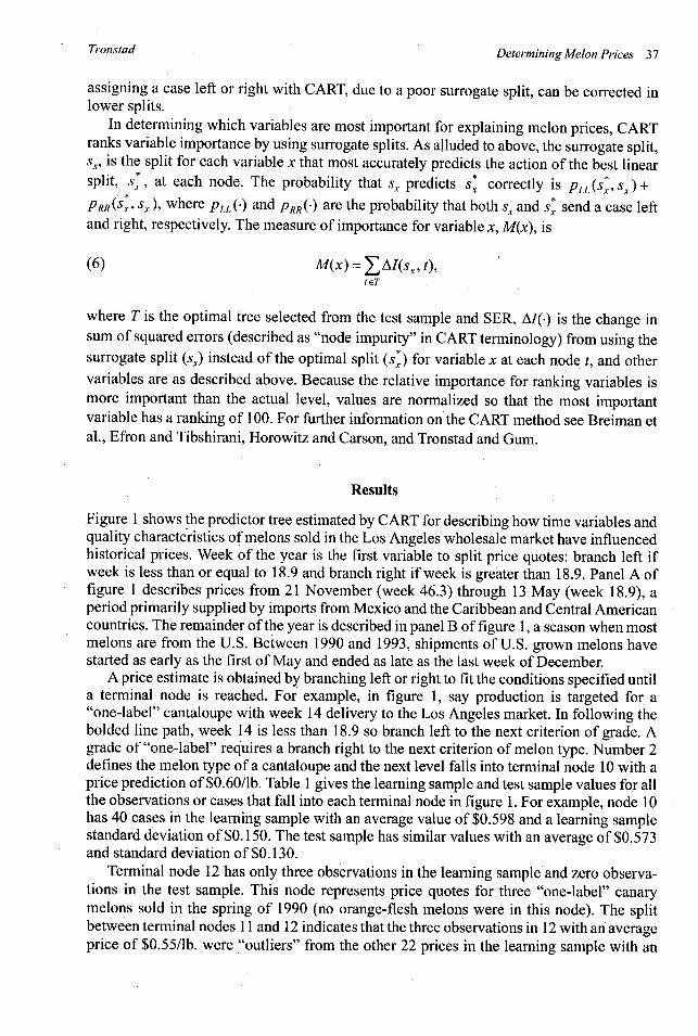
assigning a case left or right with CART, due to a poor surrogate split, can be corrected inlower splits.

In determining which variables are most important for explaining melon prices, CARTranks variable importance by using surrogate splits. As alluded to above, the surrogate split,s,, is the split for each variable x that most accurately predicts the action of the best linearsplit, s, at each node. The probability that sx predicts sx correctly is PLL(Sx,Sx)+

PRR (S, sx ), where PLL (.) and PRR(') are the probability that both sx and Sx send a case leftand right, respectively. The measure of importance for variable x, M(x), is

(6) M(x) = 'AI(x, t),teT

where T is the optimal tree selected from the test sample and SER, AI(-) is the change insum of squared errors (described as "node impurity" in CART terminology) from using thesurrogate split (sr) instead of the optimal split (s) for variable x at each node t, and othervariables are as described above. Because the relative importance for ranking variables ismore important than the actual level, values are normalized so that the most importantvariable has a ranking of 100. For further information on the CART method see Breiman etal., Efron and Tibshirani, Horowitz and Carson, and Tronstad and Gum.

Results

Figure 1 shows the predictor tree estimated by CART for describing how time variables andquality characteristics of melons sold in the Los Angeles wholesale market have influencedhistorical prices. Week of the year is the first variable to split price quotes: branch left ifweek is less than or equal to 18.9 and branch right if week is greater than 18.9. Panel A offigure 1 describes prices from 21 November (week 46.3) through 13 May (week 18.9), aperiod primarily supplied by imports from Mexico and the Caribbean and Central Americancountries. The remainder of the year is described in panel B of figure 1, a season when mostmelons are from the U.S. Between 1990 and 1993, shipments of U.S. grown melons havestarted as early as the first of May and ended as late as the last week of December.

A price estimate is obtained by branching left or right to fit the conditions specified untila terminal node is reached. For example, in figure 1, say production is targeted for a"one-label" cantaloupe with week 14 delivery to the Los Angeles market. In following thebolded line path, week 14 is less than 18.9 so branch left to the next criterion of grade. Agrade of "one-label" requires a branch right to the next criterion of melon type. Number 2defines the melon type of a cantaloupe and the next level falls into terminal node 10 with aprice prediction of $0.60/lb. Table 1 gives the learning sample and test sample values for allthe observations or cases that fall into each terminal node in figure 1. For example, node 10has 40 cases in the learning sample with an average value of $0.598 and a learning samplestandard deviation of $0.150. The test sample has similar values with an average of $0.573and standard deviation of $0.130.

Terminal node 12 has only three observations in the learning sample and zero observa-tions in the test sample. This node represents price quotes for three "one-label" canarymelons sold in the spring of 1990 (no orange-flesh melons were in this node). The splitbetween terminal nodes 11 and 12 indicates that the three observations in 12 with an averageprice of $0.55/lb. were "outliers" from the other 22 prices in the learning sample with an

Tronstad


en

T

0%

E0

Ch

.0

U)

Q)

s

cl

(A

pa

ir.

0.;0.

Pa

Li

a)

oaF~a)

o

CUU

0:

(U

(cU

cd 0asCU a

OC

cd

CC Cfl

$ "

0

a)-:

:3

a)0

eD .

04 Y

OC

c. CU

a4c

05:

0

4-aCd

Cd

VI a

a

38- July 1995

.n)

co

od

U4)

To

o

o0

U)0

1d

¢

cd

UItu

O,


N(A a,, If 00 tn CT \o

tl- tl- CIA r- f\ 0

C \.o - *i 'St a\ 00

cn

M ".0 O \ (71 00 C)Itt Cc M00 M 'IO

t-- w; vt t

U)O

CZU

L4 CZ

U) EQ O d

0 r--4 r--

(UIN

-4 '-

W~

> C") -tbli d d

1- N It .4) -4 C C

> ul \d , O

O , ID Cf)

Fte CcN 00

-4 -4 '-4 0

~--4 'RI ON eqC7\ C) t- m

tt; kl \16 vl

m ~~ 3ECu-4

c d0 id C)

U c~ Cu "C E~~~Cc~~~ c ~ >,cOUOU~~

c ,* C's cc) ~ s Cd C

u u u u~~~~~~~-

0 3

U

> CI)> W)

0

4-

CO

0

cr

a,

oo00

r.

bO

cd

-

.4

1-

5-00o

04.2

r-

40

CZ

w-4cis

.4

2:1

Oa"000

Tronstad


Table 1. Number of Cases, Average Values, and Sample Standard Deviations by TerminalNode for Learning and Test Sample Values Given in Figure 1

Learning Sample Test SampleAvg. SD Avg. SD

Node No. Cases ($/lb.) ($/lb.) No. Cases ($/lb.) ($/lb.)

1

2

3

4

5

6

7

8

9

10

11

12

13

14

15

16

17

18

19

20

21

22

23

24

25

26

27

28

29

30

31

32

33

34

35

Total

160

40

308

80

60

137

82

109

41

40

22

3

298

125

188

160

13

61

332

484

52

17

59

133

48

60

39

58

77

51

43

12

11

11

69

3483

0.293

0.580

0.403

0.322

0.437

0.545

0.394

0.602

0.472

0.598

0.892

0.550

0.156

0.204

0.267

0.325

0.714

0.425

0.186

0.257

0.327

0.496

0.253

0.313

0.310

0.441

0.460

0.279

0.396

0.345

0.484

0.689

0.311

0.543

0.617

0.060

0.150

0.077

0.084

0.120

0.150

0.086

0.150

0.160

0.150

0.150

0.024

0.052

0.073

0.080

0.100

0.170

0.100

0.060

0.067

0.050

0.048

0.054

0.073

0.052

0.073

0.110

0.110

0.130

0.097

0.100

0.072

0.090

0.044

0.120

61

20

161

40

44

65

48

60

21

26

16

0

144

67

100

76

7

29

137

208

22

12

22

54

25

45

22

21

34

30

21

7

9

5

44

1703

0.308

0.561

0.394

0.328

0.402

0.523

0.401

0.596

0.473

0.573

0.825

0.157

0.179

0.282

0.358

0.568

0.429

0.189

0.261

0.333

0.461

0.310

0.325

0.330

0.421

0.441

0.320

0.378

0.331

0.463

0.576

0.346

0.588

0.626

0.093

0.150

0.085

0.087

0.160

0.140

0.081

0.160

0.150

0.130

0.170

0.050

0.070

0.097

0.120

0.160

0.087

0.050

0.071

0.051

0.110

0.100

0.066

0.054

0.068

0.086

0.120

0.120

0.088

0.085

0.039

0.081

0.016

0.180

40 July 1995


average price of $0.892/lb. Given the small number of cases, it is not surprising that no caseswere found in the test sample. A procedure such as least absolute deviations rather thanleast-squares regression removes these "outliers" from being in their own node. But theseoutliers are salient features of the data by regression criteria since they were sorted into theirown terminal node, even though their relative numbers are small.

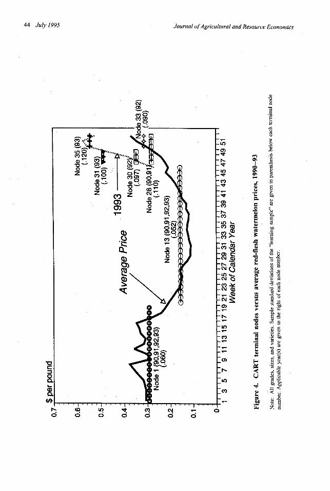
Figures 2, 3, and 4 plot estimated CART terminal nodes versus average cantaloupe,honeydew, and watermelon prices by week of calendar year.8 These figures illustrate theimportance of seasonality for melon prices. Both the average price and CART terminal nodesplotted demonstrate how prices can plummet after 13 May. This sharp drop reflects the firstlarge influx of new crop shipments from temperate areas of California, Florida, and Texas,plus continued imports from Mexico and Central America. It is not surprising that growersseek out warmer microclimates and use mulches or foams in an effort to achieve a harvestone or two weeks ahead of the spring price drop.

Red-flesh watermelon and mayan melon prices bottom out for all years after week 18.9at around $0.16/lb. and remain there until late fall. CART gives these two melon types thesame price for all years between weeks 18.9 and 46.3, the longest period for all melons.Prices continue to drop for other melon types until week 27.2, 11 July, when they hit bottomfor the year. Prices are most stable from year to year during the midsummer season, betweenweeks 27.2 and 39.7. During this period, terminal price nodes for all melons (i.e., 13, 19,20, 21, and 22) are the same for all years. Yearly price uncertainty is lower for these weeksthan any other period, but prices are least favorable then too. In considering all melon types,when week is less than 18.9 or greater than 46.3 (i.e., panel A), several terminal nodes yielda price-predictor that is greater than $0.50/lb. But for the period dominated by U.S.production (i.e., between 13 May and 21 November, which is presented in panel B), onlyone terminal node is above $0.50/lb., node 17. This node only includes "specialty melons"(canary, casaba, crenshaw, orange-flesh, persian, and santa claus) and is for a very shortwindow, between 13 May and 1 June, in 1990 and 1991.

Melon prices start to increase in the fall around 6 October (week 39.7), albeit moregradually than the price drop in the spring. Terminal nodes for shorter time periods in thefall than spring reflect the more gradual price increase. U.S. melon supplies increase in thespring more sharply with the new crop than production drops off in the fall. Melons areplanted only after minimum soil temperatures have been reached. Few heat units accumulatein early spring so that most melons are ready for harvest at about the same time, even ifplantings are a few weeks apart. Also, a light freeze in the spring would kill most seedlings,but many vines may keep producing after a light freeze in the fall. Post-harvest life alsoappears to affect how quickly prices increase in the fall. Cantaloupes have the shortestpost-harvest life and they exhibit the sharpest price increase in the fall.

A price premium was most consistently exhibited for crenshaw, orange-flesh, and sharlynmelons. Red-flesh watermelons and mayan melons were at the lowest price level ($0.156/lb.for node 13) for most of the U.S. harvest season. Seedless watermelons receive a premiumrelative to red-flesh watermelons, except after week 46.3. For other weeks, the premiumranged anywhere from a high of $0.25/lb. (weeks between 4.85 and 13.1 for 1990 and 1992)to a low of $0.05/lb. (weeks between 18.9 and 27.2 for 1992 and 1993).

Cantaloupe prices plotted are for a size number less than 21.58 [i.e., 16.064 + (1.07)(5.155)] and all grades except "one-label."

Honeydew and watermelon prices reflect a good quality grade with a size number less than 8.80 for honeydews and all sizesfor watermelons. Average prices were calculated by first taking the average of all price quotes for each week of a year. Thenthe average of each week for all years was taken so that each year would have equal weight.

Tronstad


L_

(I)>.

C

"o

0)

-I

U)a)

0c,)

\0

ci

IC,

0

ow

W-w

*,)

0

C's

I.-

CIOro3

Q)

rA4)

Po0

II&W

rD

C)

4-

*b

..

¢1

E

i-

d.

o IS

Cd

O g

a-

0

O

S a.

,n 41

* 0

o 9

ce o

a

L), .

_ a )

d2

42 July 1995

Tronstad

0)0)6


Cda)

0

cr

a

Cd

C1

§

f) S

I o

§ e 1

> *B 'RQ

bc >

Cd" I

m ed

q o*0

00

o, I

Qc C CC

C4 C

*Cf II

Journal of Agricultural and Resource Economics

L..Qs

0)

CI

0)cou,

C)

r,

*ON0oCN

uoN

Le

.*

JA

Q

QC:

4)

1.0

Li

0

C(

0

1

Lo

0

CZ

-o

0

I.0

C)

Ca

WC)

0C's

-D

r.

Cd

4-

0

4)bO

C)

'4C)

40.2

CC

C's

C)

a.CA C)

N- .0

t~000 '

.2·f:/ *S

a 0a

.014 40

44 July 1995


CART classified honeydew and cantaloupe prices in the same terminal nodes, exceptfor a few cases, as shown in figures 1,2, and 3. In May and June of 1992 and 1993, honeydewprices are estimated slightly higher than cantaloupes (i.e., nodes 15 vs. 14). But in the latefall of 1990, 1991, and 1992, cantaloupe prices are estimated higher (i.e., nodes 26 vs. 25,and nodes 29 vs. 28). The first diversion is probably from the earlier maturity of somecantaloupe varieties, while the latter probably reflects a shorter post-harvest life of canta-loupes than honeydews.

Price splits for grade occur only for "one-label" versus all "other grades." Splits occurwhen week is less than 18.9, or between weeks 27.2 and 39.7. This result suggests that"one-label" grades receive a premium only for limited time periods, and no detectablediscount is received for grades that are worse than good quality. Because little grade variationoccurs (recall that only 3.8%, or 197 price quotes make up the three poorest grades), pricesensitivity to poorer grades may have been overwhelmed by sheer numbers. But CART canisolate a few price quotes, as in terminal node 12, suggesting that price quotes for the poorergrades were not overwhelmed by absolute numbers.

Following all "one-label" versus "other-grade" splits is a binary split associated withmelon type. Crenshaw, orange-flesh, and sharlyn show a significant premium for "one-label"over other grades. A premium for "one-label" orange-flesh appears for weeks less than 18.9but not for weeks between 27.2 and 39.7. No "one-label" sharlyn melon price quotes weregiven for week less than 18.9. CART arbitrarily places these and other categorically missingmelon types "left." Arbitrarily placing absent categories from the learning sample to the leftcauses no harm as long as the specified categories continue to remain nonexistent. But thisis a shortcoming of the data and CART approach if melon production were targeted for"one-label" sharlyn melons when week is less than 18.9. The data have no "one-label"sharlyn when week is less than 18.9, and the CART algorithm fails to associate the pricepremium for weeks 27.2 to 39.7 with week less than 18.9. Due to this lack of associationand nonlinear flexibility inherent in the CART method, special caution needs to be given formaking extrapolations beyond the data. Price predictions are denoted in brackets, in figure1 for node characteristics specified that have no price quotes in the learning or test samples.This happens only for specialty melon types during specific time periods in the late fall,winter, and early spring months.

A price split for size was identified only when week was less than 18.9 and for crenshaw,mayan, and orange-flesh melon types. The two size splits identified were both for a sizenumber that was almost one standard deviation (0.792 and 1.33) above their respectiveaverage sizes. This indicates that no price premium was identified for melons larger thanaverage size, size, nce smaller numbers reflect larger melons. A binary split associated with asize number less than zero in figure 1 would be necessary for melons larger than average toreceive a premium. A discount for small size does not occur until some specialty melons areabout one standard deviation in size less than average. Size appears not to have a majorinfluence on melon prices.

The relative importance of variables for explaining melon prices is as follows: week(100), type of melon (76), year (45), size (40), grade (34), and container (18). As depictedin the predictor tree and relative importance ranking, seasonality or week is the mostimportant factor that determines melon prices with melon type not far behind. Year is next,reflecting that plantings and weather vary significantly from one year to the next. Both sizeand grade splits occur only twice in the price-predictor tree. But the relative importancevariable is higher for size than grade, indicating that size has better surrogate splits than

Tronstad


grade. Shipping container ranks at the bottom, and this is consistent with no container splitsidentified in the price-predictor tree.

How good is the overall fit of the nonparametric CART procedure? The coefficient ofdetermination orR2 (Kmenta) was calculated at 0.6795 for all melon prices using the learningsample predictors from figure 1 or table 1.9 This compares favorably with an R2 of 0.6061calculated from a parametric ordinary least squares (OLS) regression equation with dummyvariables for melon type, year, week rounded to the nearest integer (0 to 53), grade, container,and the continuous size variable. In total, 73 dummy variables, size, and a constant termwere included in the OLS regression.' The number of dummy variables in the OLSregression are more than double the binary splits (34) or terminal nodes (35) in the CARTpredictor tree. The mean absolute percent error was calculated at 22.71 for CART and 27.27for the OLS regression. CART performed better since it allows for interactions betweenvariables. For example, the premium for seedless watermelons relative to other melon typescan be higher for some weeks than other weeks. Without interactive dummy variables in theOLS regression, the premium for seedless watermelons is fixed constant for every week ofthe year.

Similarly, if the overall price level for cantaloupes starts out high as in January 1991, thisis no indication that weeks to follow for 1991 will be at a seasonally higher or lower pricethan previous years. Prices for a year are never always above or below the seasonal pricequotes of other years (figs. 2, 3, and 4). Supply shifts from one week to the next, reflectingthe perishable nature of the crop, changes in geographic production, and relatively inelasticsupply for a given week. Prices are grouped together for all years only between the weeksof 27.2 and 41.2 (terminal nodes 19,23, and 13). Dummy variables are much more amenablefor capturing yearly effects of crops that are on an annual production and storage cycle ratherthan a commodity like fresh melons. Thus, a strength of the CART approach appears to liewith its ability to identify interactions between discrete variables without requiring an undulylarge number of dummy variables as may be the case for a parametric regression equation.

Concluding Comments

CART, a computer intensive nonparametric regression procedure, was used to determinehow melon type, size, grade, shipping container, week, and year influence melon prices. The"relative importance" of variables calculated by CART ranked week (100), type of melon(76), year (45), size (40), grade (34), and shipping container (18) as the most-to-leastimportant factors. Given the importance of time variables, parametric procedures may bejustified in focusing only on seasonality for a longer series of data, even if the data representjust one grade, size, and type of melon.

A price-predictor tree constructed by CART with 34 binary splits, or 35 terminal nodes,explained melon prices favorably to an OLS regression equation with 73 dummy variables,size, and a constant term. The mean absolute percent error was 22.71 for CART and 27.27for the OLS regression. Similarly, the R2, or coefficient of determination, was 0.6795 forCART and 0.6061 for the OLS regression. CART performed better since it allows for

9R2 values are 0.6051 and 0.7600 for predictor trees with 19 (SER of 7) and 89 (SER of 3) terminal nodes, respectively.10When size specifications were missing from watermelon quotes, the average size for all watermelons was used instead.

Results were the same as regressing size on all other variables and then using these estimates of size for missing values.Interaction dummy variables (e.g., week multiplied by year) would have been unmanageable if all were considered as

variables in the OLS regression.

46 July 1995


interactions between discrete variables. Allowing for these interactions in the OLS regres-sion would have required an unduly large number of interaction dummy variables.

Crenshaw, orange-flesh, and sharlyn melons exhibited the most consistent premiums formelon type, while red-flesh watermelon and mayan melons generally received a discount.No premium was found for melons larger than average. Discounts for small sizes were foundonly for limited melon types and time periods. The only grade price differential detectedwas for a "one-label" grade associated with limited melon types and time periods. Year wasan important factor for all time periods except between 11 July and 6 October.

Melon prices show their first big price drop in the spring after 13 May. Most melon pricesdrop further until they reach bottom at around 11 July. Prices are the lowest and mostpredictable between 11 July and 6 October. After 6 October, prices start to increase, but moregradually than they drop in the spring. Most melon prices peak in mid-December.

[Received June 1994; final version received January 1995.]

References

Bowman, K. R., and D. E. Ethridge. "Characteristic Supplies and Demands in a Hedonic Framework: U.S. Marketfor Cotton Fiber Attributes." Amer J. Agr. Econ. 74(1992):991-92.

Breiman, L., J. H. Friedman, R. A. Olshen, and C. J. Stone. Classification and Regression Trees. Belmont CA:Wadsworth Publishing Co., 1984.

Brorsen, B. W., W. R. Grant, and E. M. Rister. "A Hedonic Price Model for Rice Bid/Acceptance Markets." AmerJ. Agt: Econ. 66(1984): 156-63.

Collette, A. W., and G. B. Wall. "Evaluating Vegetable Production for Market Windows as an Alternative forLimited Resource Farmers." S. J. Agr Econ. 10(1978): 189-93.

Efron, B., and R. Tibshirani. "Statistical Data Analysis in the Computer Age." Science 253(1991):390-95.Epple D. "Hedonic Prices and Implicit Markets: Estimating Demand and Supply Functions for Differentiated

Products." J. Polit. Econ. 95(1987):59-80.Ethridge, D. E., and B. Davis. "Hedonic Price Estimation for Commodities: An Application to Cotton." West. J.

Agr Econ. 7(1982):293-300.Goodwin, H. L., Jr., S. W. Fuller, O. Capps, Jr., and 0. W. Asgill. "Factors Affecting Fresh Potato Price in Selected

Terminal Markets." West. J. Agr Econ. 13(1988):233-43.Hanemann, W. M. "Quality and Demand Analysis." In New Directions in Econometric Modeling and Forecasting

in U.S. Agriculture, ed., G. C. Rausser. New York: Elsevier Science Publishing Co., 1982.Horowitz, J. K., and R. T. Carson. "A Classification Tree for Predicting Consumer Preferences for Risk

Reduction." Amer: J. Agr: Econ. 73(1991):1416-421.Jones, L. E. "The Characteristics Model, Hedonic Prices, and the Clientele Effect." J. Polit. Econ.

96(1988):551-67.Kmenta, J. Elements of Econometrics. New York: Macmillan Publishing Company Incorporated, 1971.Lancaster, K. J. Consumer Demand: A New Approach. New York: Columbia University Press, 1971.Lenz, J. E., R. C. Mittelhammer, and H. Shi. "Retail-Level Hedonics and the Valuation of Milk Components."

Amer. J. Agr. Econ. 76(1994):492-503.Lucas, R. E. B. "Hedonic Price Functions." Econ. Inquiry 13(1974):157-78.Rosen, S. "Hedonic Prices and Implicit Market Product Differentiation in Pure Competition." J. Polit. Econ.

82(1974):34-55.The Packer, Produce Services Sourcebook '93. Vance Publishing Corp., 1993.Tronstad, R., and R. Gum. "Cow Culling Decisions Adapted for Management with CART." Amer. J. Agr. Econ.

76(1994):237-49.Tronstad, R., L. S. Huthoefer, and E. Monke. "Market Windows and Hedonic Price Analyses: An Application to

the Apple Industry." J. Agr and Resour Econ. 17(1992):314-22.U. S. Department of Agriculture, Federal State Market News Service. Los Angeles Wholesale Fruit and Vegetable

Report, Weekly, 3 January 1990 through 28 December 1993.Unnevehr, L. J., and S. Bard. "Beef Quality: Will Consumers Pay for Less Fat?" J. Agr and Resour. Econ.

18(1993):288-95.

Tronstad

48 July 1995 Journal ofAgricultural and Resource Economics

Veeman, M. "Hedonic Price Functions for Wheat in the World Market: Implications for Canadian Wheat ExportStrategy." Can. J. Agr Econ. 35(1987):535-52.

Wahl, T. 1., H. Shi, and R. C. Mittelhammer. "A Hedonic Price Analysis of the Quality Characteristics of JapaneseWagyu Beef." Selected paper, WAEA annual meetings, Edmonton, Alberta, 11-14 July 1993.

Waugh, F. V. "Quality Factors Influencing Vegetable Prices." J. Farm Econ. 10(1928):185-96.Wilson, W. W. "Hedonic Prices in the Malting Barley Market." West. J. Agr Econ. 9(1984):29-40.

importance of melon type, size, grade, container,...

Documents