Importance sampling the union of rare events

with an application to power systems analysis

Art B. OwenStanford University

Yury MaximovLos Alamos National Laboratory

Michael ChertkovLos Alamos National Laboratory

February 2018

Abstract

We consider importance sampling to estimate the probability µ of aunion of J rare events Hj defined by a random variable x. The samplerwe study has been used in spatial statistics, genomics and combinatoricsgoing back at least to Frigessi and Vercellis (1985). It works by samplingone event at random, then sampling x conditionally on that event happen-ing and it constructs an unbiased estimate of µ by multiplying an inversemoment of the number of occuring events by the union bound. We provesome variance bounds for this sampler. For a sample size of n, it has avariance no larger than µ(µ − µ)/n where µ is the union bound. It alsohas a coefficient of variation no larger than

√(J + J−1 − 2)/(4n) regard-

less of the overlap pattern among the events. Our motivating problemcomes from power system reliability, where the phase differences betweenconnected nodes have a joint Gaussian distribution and the J rare eventsarise from unacceptably large phase differences. In the grid reliabilityproblems even some events defined by 5772 constraints in 326 dimensions,with probability below 10−22, are estimated with a coefficient of variationof about 0.0024 with only n = 10,000 sample values.

1 Introduction

In this paper we consider a mixture importance sampling strategy to estimatethe probability that one or more of a set of rare events takes place. The sam-pler repeatedly chooses a rare event at random, and then samples the systemconditionally on that one event taking place. For each such sample, the totalnumber of occuring events is recorded and a certain reciprocal moment of themis used in the estimate.

This method is a special case of an algorithm in Adler et al. (2012) forcomputing exceedance probabilities of Gaussian random fields. It was usedearlier by Shi et al. (2007) and Naiman and Priebe (2001) for extrema of genomic

1

arX

iv:1

710.

0696

5v2

[st

at.C

O]

27

Feb

2018

scan statistics. Priebe et al. (2001) used it for extrema of some spatial statisticinvolving marked point processes. The earliest use we know is Frigessi andVercellis (1985) who used it to estimate the cardinality of the union of a givenlist of finite sets. The above cited papers refer to this method as importancesampling. To distinguish it from other samplers, we will call it ALOE for “AtLeast One rare Event”.

We develop general bounds for the variance of the ALOE importance sam-pler, and for its coefficient of variation. It has a sampling standard deviationthat is no more than some modest multiple of the event probability. This is anespecially desirable property in rare event settings. For background on impor-tance sampling of rare events see L’Ecuyer et al. (2009).

Our motivating context is the reliability of the electrical grid when subjectto random inputs, such as variable demand by users and variable production,as occurs at wind farms. The rare events describe unacceptably large electricalphase differences at pairs of connected nodes in the grid.

It is common to use a simplified linear direct current (DC) model of theelectrical grid, because the equations describing alternating current (AC) aresignificantly more difficult to work with, and some authors (e.g., Van den Berghet al. (2014)) find that there is little to be gained from the complexity of anAC model. This DC model is presented in Sauer and Christensen (1984) andStott et al. (2009). It is also common to model the randomness in the grid asGaussian, especially over short time horizons.

We make both of these simplifications: linearity and Gaussianity. The prob-ability we consider can then be written

µ = Pr(∪Jj=1Hj

), Hj = xTωj > τj, where x ∼ N (η,Σ). (1)

Section 2 introduces more notation for problem (1) and develops the ALOEsampler as an especially convenient version of mixture importance sampling. Inthis setting we can compute the union bound µ =

∑Jj=1 Pr(Hj) > µ. Theorem 1

proves that the ALOE estimate µ has variance at most µ(µ− µ)/n when n IIDsamples are used. This can be much smaller than µ(1− µ)/n which arises fromsampling the nominal distribution of x. Section 3 discusses some further sam-pling properties of our estimator that hold without the Gaussian assumption.When there are J events, the variance of µ is at most (J + 1/J − 2)µ2/(4n)when the system is sampled n times. Section 4 compares ALOE to a state ofthe art code mvtnorm (Genz et al., 2017) for estimating the probability that amultivariate Gaussian of up to 1000 variables with arbitrary covariance belongsto a given hyperrectangle. ALOE is simpler and extends to higher dimensions.When we studied rare event cases, ALOE was more accurate. In our examplesthat are not rare events, mvtnorm was more accurate. Section 5 describes thepower system application. Section 6 contains some discussions. The appendixproves Theorem 1 for any set of J events, not just those given by a Gaussiandistribution. The theorem applies so long as we can sample conditionally onany one event Hj and then determine which other events H` also occur. Wefinish this section with some comments and some references.

2

One common way for rare event sampling to be inaccurate is that we mightfail to obtain any points where the rare event happens. That leads to a severeunder-estimation of the rare event probability. In ALOE, the correspondingproblem is the failure to sample any points where two or more of the rareconstituent events occur. In that case ALOE will return the union bound asthe estimated rare event probability instead of zero. That is also a settingwhere the union bound is likely to be a good approximation. So ALOE isrobust against severe underestimates of the rare event probability. The secondcommon problem for rare event sampling is an extreme value of the likelihoodratio weighting applied to the observations. In ALOE, the largest possibleweight is only J times as large as the smallest one.

Our sampler is closely related to instanton methods in power systems en-gineering. See Chertkov, Pan et al. (2011), Chertkov, Stepanov et al. (2011),and Kersulis et al. (2015). Out of all the configurations of random inputs toa system, the most probable one causing the failure is called the instanton.When there are thousands of failure types there are correspondingly thousandsof instantons, each one a conditional mode of the distribution of x. Our initialthought was to do importance sampling from a mixture of distributions, witheach mixture component defined by shifting the Gaussian distribution’s meanto an instanton. By sampling conditionally on an event, ALOE avoids wastingsamples outside the failure region. By conditioning instead of shifting, we getbetter control over the likelihood ratio in the importance sampler.

ALOE is a form of multiple importance sampling. Multiple importancesampling originated in computer graphics (Lafortune and Willems, 1993; Veachand Guibas, 1994). Owen and Zhou (2000) found a useful way to combine itwith control variates defined by the mixture components. Elvira et al. (2015a,b)investigate computational efficiency of some mixture importance sampling andweighting strategies.

We do not consider self-normalized importance sampling (SNIS) in this pa-per. SNIS is useful in settings where we can compute an unnormalized versionof our target density but cannot sample from it efficiently, if at all. SNIS iscommon in Bayesian applications (Liu, 2001, Chapter 2). For a recent adaptiveversion of SNIS, see Cornuet et al. (2012). In estimating rare event probabilities,the optimal sampler for SNIS can be shown to place half of its probability in therare event and half outside the rare event, while the optimal plain IS estimatorplaces all of its probability on the rare event. The best coefficient of variationfor rare event estimation under SNIS is asymptotically 2/

√n. Ordinary impor-

tance sampling can attain much smaller variances, and so we focus on it for therare event problem.

2 Gaussian case

For concreteness, we present ALOE first for Gaussian random variables. Welet x ∈ Rd have the standard Gaussian distribution, N (0, I), deferring generalGaussians to Section 2.1. We are interested in computing the probability that

3

−10 −5 0 5 10

−6

−4

−2

02

46

c(−

7, 6

)

Figure 1: The solid circles contain 10%, 20% up to 90% of the N (0, I) distri-bution. The dashed circles contain all but 10−k of the probability for 3 6 k 6 7.The six solid lines denote half-spaces. The solid points are the correspondingconditional modes (instantons). The rare event of interest is x in the shadedregion, when x ∼ N (0, I).

x lies outside a polytope P. In our motivating applications, the interior of thepolytope defines a safe operating region and we assume that x 6∈ P is a rareevent. For j = 1, . . . , J , define half-spaces

Hj = x | ωTj x > τj

where each τj ∈ R and ωj ∈ Rd, with ωTj ωj = 1. Then P = ∩Jj=1H

cj and we

want to find µ = Pr(x ∈ H) where H = ∪Jj=1Hj = Pc. The set P is convex andnot necessarily bounded. Ordinarily τj > 0, because we are interested in rareevents.

The setting is illustrated in Figure 1 for J = 6 half-spaces. In that example,two of the half-spaces have their conditional modes inside the union of the otherhalf-spaces. One of those half-spaces is entirely included in the union of theothers.

Letting Pj = Pr(x ∈ Hj) = Φ(−τj), we know that

max16j6J

Pj =: µ 6 µ 6 µ :=

J∑j=1

Pj .

The right hand side is the union bound which is sometimes very conservativeand sometimes quite accurate.

4

We will need to use some inclusion-exclusion formulas, so some notation forthese follows. For any u ⊆ 1:J ≡ 1, 2, . . . , J, let Hu = ∪j∈uHj , so Hj =Hj and by convention H∅ = ∅. We identify the set Hu with the functionHu(x) = 1x ∈ Hu. Next define Pu = E(Hu(x)) for x ∼ N (0, I). Let S(x) =∑Jj=1Hj(x) count the number of rare events that happen. For s = 0, 1, . . . , J ,

let Ts = Pr(S = s) give the distribution of S. We use |u| for the cardinalityof u. Our estimand is

µ = P1:J =∑|u|>0

(−1)|u|−1Pu, (2)

by inclusion-exclusion.Frigessi and Vercellis (1985) and other papers present the ALOE sampler

but do not derive it. Here we motivate it as an especially simple mixturesampler. The mixture components we use are conditional distributions qj =L(x | ωT

j x > τj), for j = 1, . . . , J . They have probability density functionsqj(x) = p(x)Hj(x)/Pj .

Let α1, . . . , αJ be nonnegative numbers summing to 1, and qα =∑Jj=1 αjqj .

A mixture importance sampling estimate of µ based on n draws xi ∼ qα is

µα =1

n

n∑i=1

p(xi)H1:J(xi)∑Jj=1 αjqj(xi)

=1

n

n∑i=1

H1:J(xi)∑Jj=1 αjHj(xi)P

−1j

. (3)

Notice that p(xi) has conveniently canceled from numerator and denominator.Although the inclusion-exclusion formula (2) contains 2J − 1 nonzero terms,each summand in the unbiased estimate in (3) can be computed at cost O(J).

We can induce further cancellation in (3) by making αj/Pj constant in j.Taking αj = α∗j ≡ Pj/µ, we get

µα∗ =µ

n

n∑i=1

H1:J(xi)∑Jj=1Hj(xi)

=µ

n

n∑i=1

1

S(xi), xi

iid∼ qα∗ , (4)

because H1:J(x) = 1 always holds for x ∼ qα∗ . The estimate (4) is a multiplica-tive adjustment to the union bound µ. The terms S(xi)

−1 range from 1 to 1/Jand so we will never get µα∗ larger than the union bound or smaller than µ/J .This is convenient because µ > µ > µ/J always holds.

Theorem 1. Let µα∗ be given by (4). Then

E(µα∗) = µ, (5)

and

Var(µα∗) =1

n

(µ

J∑s=1

Tss− µ2

)6µ(µ− µ)

n. (6)

Proof. See the appendix, where this is proved for a general set of J events, notnecessarily from Gaussian half-spaces.

5

The upper bound (6) involves the unknown µ, so it is not available forplanning purpose when we want to select n. The variance and the coefficientof variation, cv(µα∗) = Var(µα∗)1/2/µ can both be bounded in terms of knownquantities µ and µ as follows.

Corollary 1. Let µα∗ be given by (4). Then Var(µα∗) 6 µ2/(4n). If µ > µ/2then also Var(µα∗) 6 µ(µ− µ)/n. Similarly,

cv(µα∗) 61√n

min√

µ/µ− 1,√J − 1

. (7)

Proof. The claims about Var(µα∗) follow from maximizing (6) over µ ∈ [ µ, µ].

Next cv(µα∗)2 = (µ− µ)/(nµ) = (µ/µ− 1)/n. Then (7) follows because µ > µand µ > µ/J .

A rare event estimator has bounded relative error if cv(µ) remains boundedas one takes the limit in a sequence of problems (Asmussen and Glynn, 2007,Chapter VI). The sequence is typically one where the event of interest becomesincreasingly rare. Corollary 1 provides a bounded relative error property forALOE in any sequence of problems where J/n is uniformly bounded.

The union bound can be written

µ =

J∑j=1

Pr(Hj(x)) =

J∑j=1

∑u⊆1:J

E(Hu(x)Hc

−u(x))1j∈u =

J∑s=1

sTs.

That is µ = E(S(x)) = µE(S(x) | S(x) > 0) and so we may write (6) as

Var(µα∗) =µ2

n

(E(S | S > 0)E(S−1 | S > 0)− 1

). (8)

We will use (8) in Section 3 to get additional bounds.

2.1 General Gaussians

Now suppose that we are given y ∼ N (η,Σ) and the half-spaces are defined byγTj y > κj . We assume that Σ is nonsingular. If it is not, then we can reducey to a subset of components whose variance is nonsingular, and write the othercomponents as linear functions of this reduced set. We also assume that we canafford to take a matrix square root Σ1/2. Now x = Σ−1/2(y − η) ∼ N (0, I),and y = η + Σ1/2x. Then the half-spaces are given by

ωTj x > τj , where ωj =

γTj Σ1/2√γTj Σγj

, and τj =κj − γTj η√γTj Σγj

,

for x ∼ N (0, I). For rare events, we will have κj > γTj η. In some of ourmotivating contexts one must optimize a cost over η. Here we remark thatchanges to η change τj but not ωj .

6

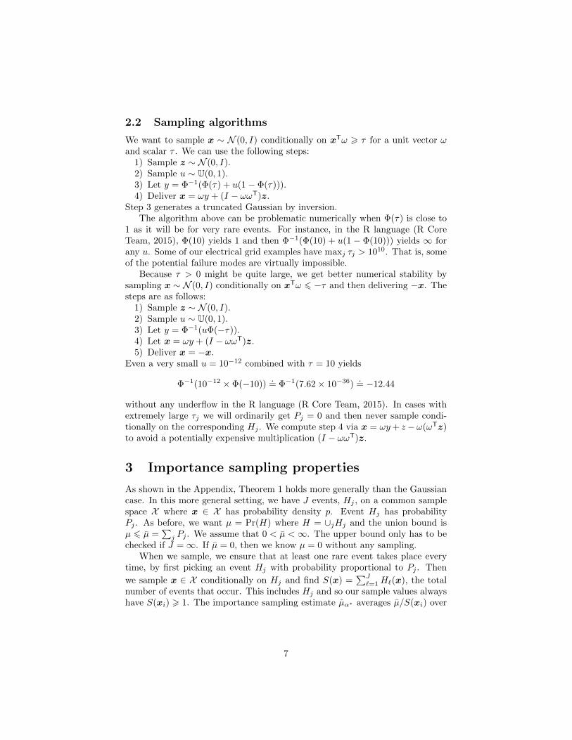
2.2 Sampling algorithms

We want to sample x ∼ N (0, I) conditionally on xTω > τ for a unit vector ωand scalar τ . We can use the following steps:

1) Sample z ∼ N (0, I).2) Sample u ∼ U(0, 1).3) Let y = Φ−1(Φ(τ) + u(1− Φ(τ))).4) Deliver x = ωy + (I − ωωT)z.

Step 3 generates a truncated Gaussian by inversion.The algorithm above can be problematic numerically when Φ(τ) is close to

1 as it will be for very rare events. For instance, in the R language (R CoreTeam, 2015), Φ(10) yields 1 and then Φ−1(Φ(10) + u(1 − Φ(10))) yields ∞ forany u. Some of our electrical grid examples have maxj τj > 1010. That is, someof the potential failure modes are virtually impossible.

Because τ > 0 might be quite large, we get better numerical stability bysampling x ∼ N (0, I) conditionally on xTω 6 −τ and then delivering −x. Thesteps are as follows:

1) Sample z ∼ N (0, I).2) Sample u ∼ U(0, 1).3) Let y = Φ−1(uΦ(−τ)).4) Let x = ωy + (I − ωωT)z.5) Deliver x = −x.

Even a very small u = 10−12 combined with τ = 10 yields

Φ−1(10−12 × Φ(−10)).= Φ−1(7.62× 10−36)

.= −12.44

without any underflow in the R language (R Core Team, 2015). In cases withextremely large τj we will ordinarily get Pj = 0 and then never sample condi-tionally on the corresponding Hj . We compute step 4 via x = ωy+ z−ω(ωTz)to avoid a potentially expensive multiplication (I − ωωT)z.

3 Importance sampling properties

As shown in the Appendix, Theorem 1 holds more generally than the Gaussiancase. In this more general setting, we have J events, Hj , on a common samplespace X where x ∈ X has probability density p. Event Hj has probabilityPj . As before, we want µ = Pr(H) where H = ∪jHj and the union bound isµ 6 µ =

∑j Pj . We assume that 0 < µ <∞. The upper bound only has to be

checked if J =∞. If µ = 0, then we know µ = 0 without any sampling.When we sample, we ensure that at least one rare event takes place every

time, by first picking an event Hj with probability proportional to Pj . Then

we sample x ∈ X conditionally on Hj and find S(x) =∑J`=1H`(x), the total

number of events that occur. This includes Hj and so our sample values alwayshave S(xi) > 1. The importance sampling estimate µα∗ averages µ/S(xi) over

7

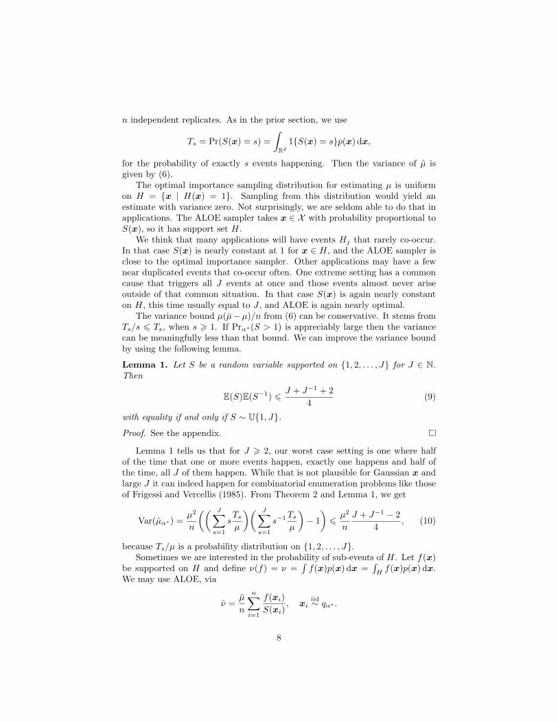
n independent replicates. As in the prior section, we use

Ts = Pr(S(x) = s) =

∫Rd

1S(x) = sp(x) dx,

for the probability of exactly s events happening. Then the variance of µ isgiven by (6).

The optimal importance sampling distribution for estimating µ is uniformon H = x | H(x) = 1. Sampling from this distribution would yield anestimate with variance zero. Not surprisingly, we are seldom able to do that inapplications. The ALOE sampler takes x ∈ X with probability proportional toS(x), so it has support set H.

We think that many applications will have events Hj that rarely co-occur.In that case S(x) is nearly constant at 1 for x ∈ H, and the ALOE sampler isclose to the optimal importance sampler. Other applications may have a fewnear duplicated events that co-occur often. One extreme setting has a commoncause that triggers all J events at once and those events almost never ariseoutside of that common situation. In that case S(x) is again nearly constanton H, this time usually equal to J , and ALOE is again nearly optimal.

The variance bound µ(µ−µ)/n from (6) can be conservative. It stems fromTs/s 6 Ts, when s > 1. If Prα∗(S > 1) is appreciably large then the variancecan be meaningfully less than that bound. We can improve the variance boundby using the following lemma.

Lemma 1. Let S be a random variable supported on 1, 2, . . . , J for J ∈ N.Then

E(S)E(S−1) 6J + J−1 + 2

4(9)

with equality if and only if S ∼ U1, J.

Proof. See the appendix.

Lemma 1 tells us that for J > 2, our worst case setting is one where halfof the time that one or more events happen, exactly one happens and half ofthe time, all J of them happen. While that is not plausible for Gaussian x andlarge J it can indeed happen for combinatorial enumeration problems like thoseof Frigessi and Vercellis (1985). From Theorem 2 and Lemma 1, we get

Var(µα∗) =µ2

n

(( J∑s=1

sTsµ

)( J∑s=1

s−1Tsµ

)− 1

)6µ2

n

J + J−1 − 2

4, (10)

because Ts/µ is a probability distribution on 1, 2, . . . , J.Sometimes we are interested in the probability of sub-events of H. Let f(x)

be supported on H and define ν(f) = ν =∫f(x)p(x) dx =

∫Hf(x)p(x) dx.

We may use ALOE, via

ν =µ

n

n∑i=1

f(xi)

S(xi), xi

iid∼ qα∗ .

8

Then by the same arguments used in the Appendix,

E(ν) = ν and Var(ν) =1

n

(µ

∫H

f(x)2p(x)

S(x)dx− ν2

).

If f(x) ∈ 0, 1, then Var(ν) 6 ν(µ − ν)/n. That is, when f describes a rareevent that can only occur if one or more of the Hj also occur, we can reduce itsMonte Carlo variance from ν(1 − ν)/n to at most ν(µ − ν)/n, in cases whereµ < 1.

4 Comparisons

Here we consider some numerical examples comparing ALOE to pmvnorm fromthe R package mvtnorm (Genz et al., 2017). This package can make use of specialproperties of the Gaussian distribution, and it works in high dimensions.

We begin by describing mvtnorm based on Genz and Bretz (2009) and apersonal communication from Alan Genz. The program computes

Pr(a 6 y 6 b) ≡ Pr(aj 6 yj 6 bj , j = 1, . . . , d)

for y ∼ N (η,Σ), where −∞ 6 aj 6 bj 6 ∞ for j = 1, . . . , d, and Σ can be

rank deficient. We can use it to compute µ = Pr(∑Jj=1 1ωT

j x > τj > 0) forx ∼ N (0, I) via

1− µ = Pr(ΩTx 6 T ) = Pr(y 6 T ), y ∼ N (0,ΩTΩ).

The code can handle dimensions up to 1000. In our context, that means atmost J = 1000 half-spaces. The dimension d can be higher. The related pmvt

function handles multivariate t random variables. The code has three differentalgorithms in it. One from Genz (2004) handles two and three dimensionalsemi-infinite regions, one from Miwa et al. (2003) is for dimensions up to 20 andthe rest are handled by an algorithm from Genz and Bretz (2009). This latteralgorithm uses a number of methods. It uses randomized Korobov lattice rulesas described by Cranley and Patterson (1976) for the first 100 dimensions, inconjunction with antithetic sampling. There are usually 8 randomizations. Formore than 100 dimensions it applies a method from Niederreiter (1972). Thereare a series of increasing sample sizes in use, and the method provides an esti-mated error (3.5 standard errors) based on the randomization. The approachis via sequential conditional sampling, after strategically ordering the variables(e.g., putting unconstrained ones first). The R package calls a FORTRAN pro-gram for the computation, so it is very fast. We use the default implementationwhich uses up to 25,000 quadrature points.

The main finding is that importance sampling is more effective when thepolytope of interest is the complement of a rare event. This is not meant tobe a criticism of pmvnorm. That code was not specifically designed to computethe complement of a rare event. The comparison is relevant because we are not

9

τ µ E((µALOE/µ− 1)2) E((µMVN/µ− 1)2)

2 1.35×10−01 0.000399 9.42×10−08

3 1.11×10−02 0.000451 9.24×10−07

4 3.35×10−04 0.000549 2.37×10−02

5 3.73×10−06 0.000600 1.81×10+00

6 1.52×10−08 0.000543 4.39×10−01

7 2.29×10−11 0.000559 3.62×10−01

8 1.27×10−14 0.000540 1.34×10−01

Table 1: Results from 100 computations of Pr(x 6∈ P(360, τ)) for variousτ . The true mean µ is very nearly exp(−τ2/2). Importance sampling is moreaccurate for large τ (rare events), while pmvnorm is more accurate for small τ .

aware of alternative code tuned for the high dimensional rare event cases thatwe need, and pmvnorm is a well regarded and widely available general solution,that seemed to us like the best off-the-shelf tool.

4.1 Circumscribed polygon

Let P(J, τ) ⊂ R2 be the regular polygon of J > 3 sides circumscribed aroundthe circle of radius τ > 0. This polygon is the intersection of Hc

j where Hj =

x ∈ R2 | ωTj x > τ where ωT

j = (sin(2πj/J), cos(2πj/J)), for j = 1, . . . , J . We

want µ = Pr(x ∈ Pc) for x ∼ N (0, I). Here we know that µ 6 Pr(χ2(2) > τ2) =

exp(−τ2/2). Also, the gap between the circle of radius τ and the circumscribedpolygon has area G(J, τ) = (J tan(π/J)−π)τ2. The bivariate Gaussian densityin this gap is at most exp(−τ2/2)/(2π). Therefore

Pr(x ∈ Pc) > exp(−τ2/2)−G(J, τ) exp(−τ2/2)/(2π)

that is

1 >Pr(x ∈ Pc)exp(−τ2/2)

> 1− G(J, 1)τ2

2π

.= 1− π2τ2

6J2,

for large J .For J = 360 and τ = 6, we have µ 6 exp(−18)

.= 1.52 × 10−8. The lower

bound is about 0.9995 times the upper bound, so we treat the upper bound asexact. Figure 2 shows histograms of 100 simulations of µ/µ using ALOE andusing pvnorm. In this case ALOE is much more accurate. The mean squarerelative error E((µ/µ−1)2) is about 800-fold smaller for ALOE than pvnorm. Wealso see that pvnorm has high positive skewness and the histogram of estimateshas most of its mass well below the mean.

Table 1 shows summary results for this problem with different values of τ .We see that pvnorm is superior when the event is not rare but ALOE is superiorfor rare events. The large error for pvnorm with τ = 5 stemmed from a smallnumber of outliers among the 100 trials.

10

ALORE

Relative estimate

Fre

quen

cy

0.96 1.00 1.04

02

46

810

Pmvnorm

Relative estimate

Fre

quen

cy1 2 3 4 5 6

010

2030

4050

60

Figure 2: Results of 100 estimates of the Pr(x 6∈ P(360, 6)), divided byexp(−62/2). Left panel: ALOE. Right panel: pmvnorm.

The upper bound in equation (6) is Var(µ) 6 µ(µ − µ)/n, from whichE((µ/µ − 1)2) 6 (µ/µ − 1)/n. For τ = 6 this yields about 0.022, which isover 20 times the actual mean squared relative error from Table 1.

It is possible that this example is artificially easy for importance sampling,due to the symmetry. Whichever half-space Hj we sample, the distribution ofoverlapping half-spaces Hk for k 6= j is the same. Two half-spaces differ fromHj by a one degree angle, two differ by a two degree angle and so on. To geta more varied range of overlap patterns, we replaced angles 2πj/360 by angles2π × p(j)/360 where p(j) is the j’th prime among integers up to 360. Thereare 72 of them, of which the largest is 359. With τ = 6 and 100 replicationsusing n = 1000 points in importance sampling, we have variance of p/ exp(−18)equal to 0.00077. The comparable figure for mvtnorm is 8.5. There were a fewoutliers there including one that was more than 6 times the union bound. Thegap between the prime angle polygon and the inscribed circle is larger than theone formed by the full polygon. Pooling all the importance sampling runs leavesan estimate of about 0.94× exp(−18) for µ. In this example, we see importancesampling working quite well without symmetry.

4.2 High dimensional half-spaces

The previous example was low dimensional and each of the half-spaces sampledhad numerous similar ones, differing in angle by a small number of degrees.Thus µ was quite a bit smaller than µ. Here we consider a high dimensionalsetting where the half-spaces have less overlap.

11

1e−08 1e−07 1e−06 1e−05 1e−04

110

010

000

Union bound

Est

imat

e / B

ound

ALOREpmvnorm

Figure 3: Results of 200 estimates of the µ for varying high dimensionalproblems with nearly independent events.

Two uniform random unit vectors ω1 and ω2 in Rd are very likely to benearly orthogonal for large d. Then xTωj > τj are nearly independent events.For independent events, we would have

Pr(x 6∈ P) = 1−J∏j=1

(1− Pj).

To make x 6∈ P a rare event, the Pj must be small and then the probabilityabove will be close to the union bound. Theorem 2 predicts good performancefor importance sampling here.

For this test 200 sample problems were constructed. The dimensions werechosen by d ∼ U20, 50, 100, 200, 500. Then there were J ∼ Ud/2, d, 2dconstraints chosen with uniform random unit vectors ωj ∈ Rd. The threshold τwas chosen so that log10 of the union bound was U[4, 8], followed by rounding totwo significant figures. Then µ was computed by importance sampling with n =1000 samples, and by pmvnorm. Figure 3 shows the results. The ALOE samplingvalue was always very close to the union bound which in turn is essentially equalto what one would see for independent events. The values from pmvnorm wereusually too small. By construction the intersection probabilities are quite rare.In importance sampling, 77.5% of the simulations had no intersections among1000 trials and the others had only a few intersections. Therefore it is clear thatthe probabilities should be close to the union bounds here. We also see evidenceof strong positive skewness for pmvnorm.

12

5 Power system infeasibility

5.1 Model

Our power system models are based on a network of N nodes, called busses.Some busses put power into the network and others consume power. The Medges in the network correspond to power lines between busses. The network isordinarily sparse, with M a small multiple of N .

The power production at bus i is pi, with negative values indicating con-sumption. For some busses, pi is tightly controlled and deterministic in therelevant time horizon. Other busses have random pi corresponding, for ex-ample, to variable consumption levels, that we treat as independent. Bussescorresponding to wind farms have random power production levels with mean-ingfully large correlations. Our models contain one special bus S, called theslack bus, at which the power is pS = −

∑i6=S pi. The total power in the system

is zero because transmission power losses are ignored in the DC approximationthat we use.

The power at all busses can be represented by the vector p = (pTF , pTR, pS)T

corresponding to fixed busses, ordinary random busses (including any correlatedones) and the slack bus. There are NF fixed busses, NS = 1 slack bus andNR = N −NF −NS random busses apart from the slack bus. We will use 1Rto denote a column vector of NR ones, and IR to denote the identity matrix ofsize NR and similarly for 1F and IF .

The power pi at bus i must satisfy the constraints

pi6 pi 6 pi. (11)

The vector p has a Gaussian distribution, determined entirely by the randomcomponents pR ∼ N (ηR,ΣRR). Therefore in the present context, pR is theGaussian random variable x from Section 2. The fixed components satisfy pF =ηF and then the slack bus satisfies pS ∼ N (ηS ,ΣSS) where ηS = −1TRηR−1TF ηFand ΣSS = 1TRΣRR1R. Because all of the randomness comes from pR, we willabbreviate ΣRR to Σ.

The node to node inductances in the network form a Laplacian matrix Bwhere Bij 6= 0 if busses i and j are connected with Bii = −

∑j 6=iBij (up to

rounding). The Laplacian is symmetric and has one eigenvalue of zero for aconnected network. It has a pseudo-inverse B+. We partition B and B+ asfollows

B =

BRR BRF BRSBFR BFF BFSBSR BSF BSS

, and B+ =

BRR BRF BRS

BFR BFF BFS

BSR BSF BSS

.

We also group B+ into three sets of columns via B+ =(B•R B•F B•S

).

The phase at bus i is denoted θi. In our DC approximation of AC powerflow, the phases approximately satisfy Bθ = p. Given the power vector p, we

13

take

θ = B+p =

BRR BRF BRS

BFR BFF BFS

BSR BSF BSS

pRpFpS

.

The phase constraints on the network are

|θi − θj | 6 θij , for i 6= j and Bij 6= 0. (12)

In our examples, all θij = θ for a single value θ such as π/6 or π/4.Let D ∈ −1, 1M×N be the incidence matrix. Each edge in the network is

represented by one row of D with an entry of +1 for one of the busses on thatedge and −1 for the other. The phase constraints are |Dθ| 6 θ componentwise.Now

Dθ = D(B•R B•F B•S

)pRpFpS

= D(B•RpR +B•F pF +B•SpS

).

The constraint that Dθ 6 θ for every edge ij can be written

DB•RpR 6 θ −DB•F pF −DB•SpS .

Now pS = −1TRpR − 1TF pF and pF = ηF , so the constraint on pR is

D(B•R −B•S1TR

)pR 6 θ −D

(B•F −B•S1TF

)ηF . (13)

We also have constraints Dθ > −θ which can be written

D(B•S1TR −B•R)pR

)6 θ +D

(B•F −B•S1TF

)ηF . (14)

Equations (13) and (14) supply 2M constraints on the random vector pR.We have also the two slack bus constraints pS 6 pS and −pS 6 −p

S, that is

−1TRpR 6 pS + 1TF ηF and 1TRpR 6 −pS

+ 1TF ηF . (15)

Finally, there are individual constraints on the random busses

pR 6 pR, and − pR 6 −pR,

componentwise.When we combine all of the constraints on pR, we get a matrix Γ with rows

γj and a vector of upper bounds K with entries κj for which the constraints areΓ× pR 6 K componentwise. Here those matrices are

Γ =

IR

−IR1TR−1TR

D(B•R −B•S1TR)

−D(B•R −B•S1TR)

, and K =

pR

−pR

−pS

+ 1TF ηF

pS + 1TF ηF

θ −D(B•F −B•S1TF

)ηF

θ +D(B•F −B•S1TF

)ηF

.

14

ω µ se/µ µ µ

π/4 3.7× 10−23 0.0024 3.6× 10−23 4.2× 10−23

π/5 2.6× 10−12 0.0022 2.6× 10−12 2.9× 10−12

π/6 3.9× 10−07 0.0024 3.9× 10−07 4.4× 10−07

π/7 2.0× 10−03 0.0027 2.0× 10−03 2.4× 10−03

Table 2: Rare event estimates for the winter peak grid. ω is the phase con-straint, µ is the ALOE estimate, se is the estimated standard error, µ is thelargest single event probability and µ is the union bound.

These are the linear constraints on pR. There are 2M phase constraints andthere are two constraints for all of the non-fixed busses, including the slack bus.These constraints can be turned into constraints Ω and T on a N (0, IR) vectoras described in Section 2.1.

5.2 Examples

We considered several model electrical grids included in the MATPOWER dis-tribution (Zimmerman et al., 2011). In each case we modeled violations of thephase constraints, and used n = 10,000 samples. For some cases we found that,under our model, phase constraint violations were not rare events. In some othercases, the rare event probability was dominated by one single phase condition:µ = maxJj=1 Pj ≈

∑Jj=1 Pj = µ. For cases like this there is no need for elab-

orate computation because we know µ is within a narrow interval [µ, µ]. Theinteresting cases were of rare events not dominated by a single failure mode.We investigate two of them.

The first is the Polish winter peak grid of 2383 busses. There were d = 326random (uncontrolled) busses and J = 5772 phase constraints. We varied ωas shown in Table 2. For ω = π/7 constraint violations are not very rare. Atω = π/4 they are quite rare. The estimated coefficient of variation is nearlyconstant over this range.

The second interesting case is the Pegase 2869 model of Fliscounakis et al.(2013). This has d = 509 uncontrolled busses and J = 7936 phase constraints.It is described as “power flow for a large part of the European system”. Theresults are shown in Table 3. We include an unrealistically large bound ω = π/2in that table, to test the limits of our approach. For ω = π/2, the standard errorgiven is zero. One half-space was sampled 9408 times, another was sampled 592times but in no instance were there two or more phase violations. The estimatereverts to the union bound. Getting 0 doubletons (S = 2) among n = 10,000tries is compatible with the true probability of a doubleton being as high as 3/n.Even if T1 = .9997 and T2 = .0003 then we would have µ = (1− (3/2)× 10−4)µinstead of µ. We return to this issue in the discussion.

In addition to the examples above we investigated IEEE case 14, IEEE case300, and Pegase 1354, which were all dominated by one failure. We considered

15

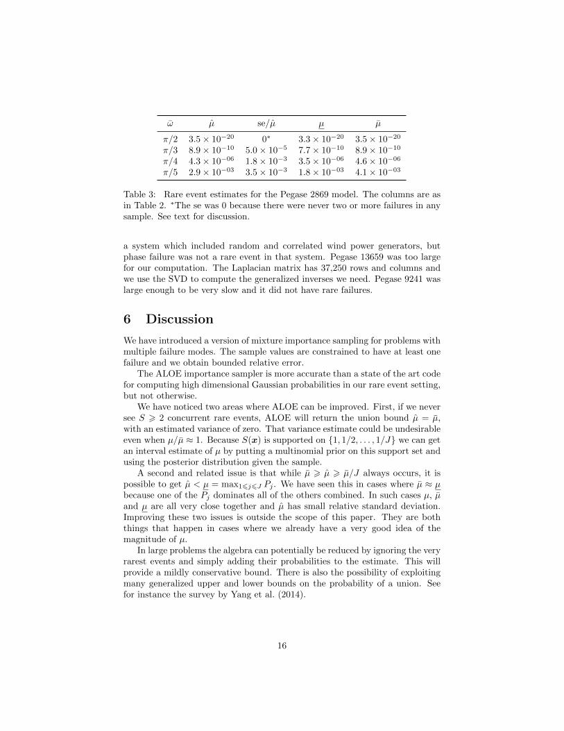
ω µ se/µ µ µ

π/2 3.5× 10−20 0∗ 3.3× 10−20 3.5× 10−20

π/3 8.9× 10−10 5.0× 10−5 7.7× 10−10 8.9× 10−10

π/4 4.3× 10−06 1.8× 10−3 3.5× 10−06 4.6× 10−06

π/5 2.9× 10−03 3.5× 10−3 1.8× 10−03 4.1× 10−03

Table 3: Rare event estimates for the Pegase 2869 model. The columns are asin Table 2. ∗The se was 0 because there were never two or more failures in anysample. See text for discussion.

a system which included random and correlated wind power generators, butphase failure was not a rare event in that system. Pegase 13659 was too largefor our computation. The Laplacian matrix has 37,250 rows and columns andwe use the SVD to compute the generalized inverses we need. Pegase 9241 waslarge enough to be very slow and it did not have rare failures.

6 Discussion

We have introduced a version of mixture importance sampling for problems withmultiple failure modes. The sample values are constrained to have at least onefailure and we obtain bounded relative error.

The ALOE importance sampler is more accurate than a state of the art codefor computing high dimensional Gaussian probabilities in our rare event setting,but not otherwise.

We have noticed two areas where ALOE can be improved. First, if we neversee S > 2 concurrent rare events, ALOE will return the union bound µ = µ,with an estimated variance of zero. That variance estimate could be undesirableeven when µ/µ ≈ 1. Because S(x) is supported on 1, 1/2, . . . , 1/J we can getan interval estimate of µ by putting a multinomial prior on this support set andusing the posterior distribution given the sample.

A second and related issue is that while µ > µ > µ/J always occurs, it ispossible to get µ < µ = max16j6J Pj . We have seen this in cases where µ ≈ µbecause one of the Pj dominates all of the others combined. In such cases µ, µand µ are all very close together and µ has small relative standard deviation.Improving these two issues is outside the scope of this paper. They are boththings that happen in cases where we already have a very good idea of themagnitude of µ.

In large problems the algebra can potentially be reduced by ignoring the veryrarest events and simply adding their probabilities to the estimate. This willprovide a mildly conservative bound. There is also the possibility of exploitingmany generalized upper and lower bounds on the probability of a union. Seefor instance the survey by Yang et al. (2014).

16

Acknowledgments

We thank Alan Genz for providing details of the mvtnorm package. We thankYanbo Tang and Jeffrey Negrea for noticing that Lemma 1 could be proved byCauchy-Schwarz, which is shorter than our original proof and also establishesnecessity. Thanks also to Bert Zwart, Jose Blanchet and David Siegmund forpointers to the literature. ABO thanks the Center for Nonlinear Studies atLos Alamos for their hospitality while he visited. The work of YM and MCwas funded by DOE/GMLC 2.0 project: “Emergency Monitoring and controlsthrough new technologies and analytics”. ABO was supported by the NSFunder grants DMS-1521145 and DMS-1407397.

References

Adler, R. J., J. H. Blanchet, and J. Liu (2012). Efficient Monte Carlo for high ex-cursions of Gaussian random fields. The Annals of Applied Probability 22 (3),1167–1214.

Asmussen, S. and P. W. Glynn (2007). Stochastic simulation: algorithms andanalysis, Volume 57. Springer Science & Business Media.

Chertkov, M., F. Pan, and M. G. Stepanov (2011). Predicting failures in powergrids: The case of static overloads. IEEE Transactions on Smart Grid 2 (1),162–172.

Chertkov, M., M. Stepanov, F. Pan, and R. Baldick (2011). Exact and effi-cient algorithm to discover extreme stochastic events in wind generation overtransmission power grids. In 2011 50th IEEE Conference on Decision andControl and European Control Conference, pp. 2174–2180.

Cornuet, J., J.-M. Marin, A. Mira, and C. P. Robert (2012). Adaptive multipleimportance sampling. Scandinavian Journal of Statistics 39 (4), 798–812.

Cranley, R. and T. N. L. Patterson (1976). Randomization of number theoreticmethods for multiple integration. SIAM Journal of Numerical Analysis 13 (6),904–914.

Elvira, V., L. Martino, D. Luengo, and M. F. Bugallo (2015a). Efficient multi-ple importance sampling estimators. IEEE Signal Processing Letters 22 (10),1757–1761.

Elvira, V., L. Martino, D. Luengo, and M. F. Bugallo (2015b). Generalizedmultiple importance sampling. arXiv preprint arXiv:1511.03095 .

Fliscounakis, S., P. Panciatici, F. Capitanescu, and L. Wehenkel (2013). Con-tingency ranking with respect to overloads in very large power systems takinginto account uncertainty, preventive, and corrective actions. IEEE Transac-tions on Power Systems 28 (4), 4909–4917.

17

Frigessi, A. and C. Vercellis (1985). An analysis of Monte Carlo algorithms forcounting problems. Calcolo 22 (4), 413–428.

Genz, A. (2004). Numerical computation of rectangular bivariate and trivariatenormal and t probabilities. Statistics and Computing 14 (3), 251–260.

Genz, A. and F. Bretz (2009). Computation of Multivariate Normal and tProbabilities. Berlin: Springer-Verlag.

Genz, A., F. Bretz, T. Miwa, X. Mi, F. Leisch, F. Scheipl, and T. Hothorn(2017). mvtnorm: Multivariate Normal and t Distributions. R package version1.0-6.

Hesterberg, T. C. (1995). Weighted average importance sampling and defensivemixture distributions. Technometrics 37 (2), 185–192.

Kersulis, J., I. Hiskens, M. Chertkov, S. Backhaus, and D. Bienstock (2015,June). Temperature-based instanton analysis: Identifying vulnerability intransmission networks. In 2015 IEEE Eindhoven PowerTech, pp. 1–6.

Lafortune, E. P. and Y. D. Willems (1993). Bidirectional path tracing. InProceedings of CompuGraphics, pp. 95–104.

L’Ecuyer, P., M. Mandjes, and B. Tuffin (2009). Importance sampling and rareevent simulation. In G. Rubino and B. Tuffin (Eds.), Rare event simulationusing Monte Carlo methods, pp. 17–38. Chichester, UK: John Wiley & Sons.

Liu, J. S. (2001). Monte Carlo strategies in scientific computing. New York:Springer.

Miwa, T., A. Hayter, and S. Kuriki (2003). The evaluation of general non-centred orthant probabilities. Journal of the Royal Statistical Society, SeriesB 65 (1), 223–234.

Naiman, D. Q. and C. E. Priebe (2001). Computing scan statistic p valuesusing importance sampling, with applications to genetics and medical imageanalysis. Journal of Computational and Graphical Statistics 10 (2), 296–328.

Niederreiter, H. (1972). On a number-theoretical integration method. Aequa-tiones Math 8 (3), 304–311.

Owen, A. B. and Y. Zhou (2000). Safe and effective importance sampling.Journal of the American Statistical Association 95 (449), 135–143.

Priebe, C. E., D. Q. Naiman, and L. M. Cope (2001). Importance samplingfor spatial scan analysis: computing scan statistic p-values for marked pointprocesses. Computational statistics & data analysis 35 (4), 475–485.

R Core Team (2015). R: A Language and Environment for Statistical Comput-ing. Vienna, Austria: R Foundation for Statistical Computing.

18

Sauer, P. W. and J. P. Christensen (1984). Active linear DC circuit models forpower system analysis. Electric machines and power systems 9 (2-3), 103–112.

Shi, J., D. O. Siegmund, and B. Yakir (2007). Importance sampling for es-timating p values in linkage analysis. Journal of the American StatisticalAssociation 102 (479), 929–937.

Stott, B., J. Jardim, and O. Alsac (2009). DC power flow revisited. IEEETransactions on Power Systems 24 (3), 1290–1300.

Van den Bergh, K., E. Delarue, and W. Dhaeseleer (2014). DC power flow inunit commitment models. Technical Report WP EN2014-12, KU Leuven.

Veach, E. and L. Guibas (1994, June 13–15). Bidirectional estimators for lighttransport. In 5th Annual Eurographics Workshop on Rendering, pp. 147–162.

Yang, J., F. Alajaji, and G. Takahara (2014). A short survey on bounding theunion probability using partial information. Technical report, University ofToronto.

Zimmerman, R. D., C. E. Murillo-Sanchez, and R. J. Thomas (2011). MAT-POWER: steady-state operations, planning, and analysis tools for power sys-tems research and education. IEEE Transactions on power systems 26 (1),12–19.

Appendix: Proofs

Proof of Theorem 2

Our motivating problem involves probabilities defined by Gaussian content ofhalf-spaces. The approach generalizes to estimating the probability of the unionof any finite set of events. We can also consider a countable number of eventswhen the union bound is finite; see remarks below. We will assume that eachevent has positive probability, but that condition can also be weakened to apositive union bound, as described at the end of this section.

For definiteness, we define our sets in terms of indicator functions of a ran-dom variable x ∈ Rd with probability density p. The same formulas work forgeneral sample spaces and the density can be with respect to an arbitrary basemeasure.

We cast our notation into this more general setting as follows. For J > 1,and j = 1, . . . , J , let the subset Hj ⊂ Rd define both the event Hj = 1x ∈ Hjand the indicator function Hj(x) = 1x ∈ Hj. For u ⊆ 1, . . . , J we letHu = ∪j∈uHj and Hu(x) = maxj∈uHj(x), with H∅(x) = 0. As before Pu =

E(Hu(x)), the number of events is S(x) =∑Jj=1Hj(x) and Pr(S = s) = Ts.

Next we introduce some further notation. We use −u for complements withrespect to 1:J , especially within subscripts, and Hc

u(x) for the complementary

19

outcome 1−Hu(x). Then Hu(x)Hc−u(x) describes the event where xj ∈ Hj if

and only if j ∈ u.If Pj > 0, then the distribution qj of x given Hj is well defined: qj(x) =

p(x)Hj(x)/Pj . If minj Pj > 0 then we can define the mixture distribution

qα∗ =

J∑j=1

α∗jqj , α∗j = Pj/µ, µ =

J∑j=1

Pj . (16)

For n > 1, our estimator of µ = Pr(S(x) > 0) is

µα∗ =µ

n

n∑i=1

1

S(xi), xi

iid∼ qα∗ . (17)

In this section, some equations include both randomness due to xi ∼ qα∗

and randomness due to x ∼ p. For section only, we use Pr∗, E∗ and Var∗ whenthe randomness is from observations xi ∼ qα∗ , while E, Pr and Var are withrespect to x ∼ p.

Theorem 2. If 1 6 J < ∞ and minj Pj > 0 and n > 1, then µα∗ definedby (16) satisfies Pr∗(µ/J 6 µα∗ 6 µ) = 1,

E∗(µα∗) = µ, (18)

and

Var∗(µα∗) =1

n

(µ

J∑s=1

Tss− µ2

)6µ(µ− µ)

n. (19)

Proof of Theorem 2. Let H(x) = max16j6J Hj(x) and H = x | H(x) = 1.If xi ∼ qα∗ , then xi ∈ H always holds. Then 1 6 S(xi) 6 J holds establishingthe bounds on µα∗ . Next

E∗

(( J∑j=1

Hj(x1)

)−1)=

J∑`=1

P`µ

∫H

H`(x)P−1` p(x)∑Jj=1Hj(x)

dx =1

µ

∫H

p(x) dx =µ

µ,

establishing (18).Because µα∗ is unbiased its variance is

1

n

(µ2E∗

((H(x1)∑Jj=1Hj(x1)

)2)− µ2

). (20)

Next

E∗(( H(x1)∑

j Hj(x1)

)2)=

J∑j=1

Pjµ

∫H

( H(x)

1 +∑` 6=j H`(x)

)2 p(x)Hj(x)

Pjdx

20

= µ−1∫H

p(x)∑Jj=1Hj(x)

dx

= µ−1∑|u|>0

1

|u|

∫Hu(x)Hc

−u(x)p(x) dx

= µ−1J∑s=1

1

sTs,

which, with (20), establishes the equality in (19). Next

µ−1J∑s=1

Tss

6 µ−1J∑s=1

Ts = µ−1(1− T0) = µ−1µ.

Finally µ2(µ−1µ)− µ2 = (µ− µ)µ, establishing the upper bound in (19).

We can generalize the previous theorem to higher moments. Our estimateis an average of µ/S(xi). The k’th moment of this quantity is

E∗(( µ

S(x1)

)k )= µk

J∑j=1

αj

∫H

S(x)−kqj(x) dx

= µkJ∑j=1

Pjµ

∫H

S(x)−kp(x)Hj(x)

Pjdx

= µk−1∫H

S(x)1−k dx

=

J∑s=1

Ts

( µs

)k−1.

Remark 1. Suppose that one of the Pj = 0 but µ > 0. In this case qj is notwell defined. However qα∗ places probability 0 on qj , so we may delete the qjcomponent without changing the algorithm and then sampling from qα∗ is welldefined.

Remark 2. Next suppose that there are infinitely many events, one for eachj ∈ N. If µ ∈ (0,∞), then qα∗ is well defined. The same proof goes through,only now sums over 1:J must be replaced by sums over N.

Proof of Lemma 1

From the Cauchy-Schwarz inequality,

1− E(S)E(S−1) = Cov(S, S−1) > −√

Var(S)Var(S−1). (21)

Now Var(S) 6 (J − 1)2/4 and Var(S−1) 6 (1− J−1)2/4 because the support ofS is in [1, J ]. Therefore

E(S)E(S−1) 6 1 +(J − 1)(1− J−1)

4=J + J−1 + 2

4.

21

Finally, the unique distribution for which Var(S), Var(S−1) and −Corr(S, S−1)all attain their maxima is U1, J.

Generalization

The lemma generalizes. If Pr(a 6 X 6 b) = 1 for 0 < a 6 b <∞ then the sameargument yields E(X)E(X−1) 6 (a/b+ b/a+ 2)/4.

22