imprecise probabilities in stochastic processes and ...gdcooma/presentations/stochastic.pdf ·...

Imprecise Probabilities inStochastic Processes and Graphical Models:

New Developments

Gert de Cooman

Ghent UniversitySYSTeMS

NLMUA2011, 7th September 2011

IMPRECISEPROBABILITY MODELS

Imprecise probability modelsSets of probability models

“An imprecise probability model is a set M of precise probability models P”

More precisely:M is a closed convex set of probabilities.

ConditioningTo condition M on an event B, we condition each precise model in M :

M |B := P(·|B) : P ∈M

Imprecise probability modelsLower and upper previsions

Consider, for a function f

P(f ) := minP(f ) : P ∈M P(f ) := maxP(f ) : P ∈M

The nonlinear functionals P and P determine M completely.

Conditioning and the Generalised Bayes RuleWhen P(B)> 0 then P(f |B) is the unique solution of the equation in x:

P(IB[f − x]) = 0.

@ARTICLEwalley2000,author = Walley, Peter,title = Towards a unified theory of imprecise probability,journal = International Journal of Approximate Reasoning,year = 2000,volume = 24,pages = 125--148

Imprecise probability modelsAccepting gambles

Consider an exhaustive set Ω of mutually exclusive alternatives ω , exactlyone of which obtains.

Subjectis uncertain about which alternative obtains.

A gamble f : Ω→ Ris interpreted as an uncertain reward: if the alternative that obtains is ω , thenthe reward for Subject is f (ω).

Let G (Ω) be the set of all gambles on Ω.

Imprecise probability modelsAccepting gambles

Subject accepts a gamble fif he accepts to engage in the following transaction, where

1. we determine which alternative ω obtains;

2. Subject receives f (ω).

We try to model Subject’s uncertainty by looking at which gambles in G (Ω) heaccepts.

Imprecise probability modelsCoherent sets of desirable gambles

Subject specifies a set D of gambles he accepts, his set of desirable gambles.D is called coherent if it satisfies the following rationality requirements:

D1. if f ≤ 0 then f 6∈D [avoiding partial loss];

D2. if f > 0 then f ∈D [accepting partial gain];

D3. if f1 ∈D and f2 ∈D then f1 + f2 ∈D [combination];

D4. if f ∈D then λ f ∈D for all non-negative real numbers λ [scaling].

Here ‘f > 0’ means ‘f ≥ 0 and not f = 0’. Walley has also argued that sets ofdesirable gambles should satisfy an additional axiom:

D5. D is B-conglomerable for any partition B of Ω:if IBf ∈D for all B ∈B, then also f ∈D [full conglomerability].

Imprecise probability modelsNatural extension as a form of inference

Since D1–D4 are preserved under arbitrary non-empty intersections:

TheoremLet A be any set of gambles. Then there is a coherent set of desirablegambles that includes A if and only if

f 6≤ 0 for all f ∈ posi(A )

In that case, the natural extension E (A ) of A is the smallest such coherentset, and given by:

E (A ) := posi(A ∪G +(Ω)).

Imprecise probability modelsLower and upper previsions

Given Subject’s coherent set D , we can define his upper and lower previsions:

P(f ) := infα : α− f ∈DP(f ) := supα : f −α ∈D

so P(f ) =−P(−f ).

– P(f ) is the supremum price α for which Subject will buy the gamble f ,i.e., accept the gamble f −α .

– the lower probability P(A) := P(IA) is Subject’s supremum rate forbetting on the event A.

Imprecise probability modelsConditional lower and upper previsions

We can also define Subject’s conditional lower and upper previsions: for anygamble f and any non-empty subset B of Ω, with indicator IB:

P(f |B) := infα : IB(α− f ) ∈DP(f |B) := supα : IB(f −α) ∈D

so P(f |B) =−P(−f |B) and P(f ) = P(f |Ω).

– P(f |B) is the supremum price α for which Subject will buy the gamble f ,i.e., accept the gamble f −α , contingent on the occurrence of B.

– For any partition B, define the gamble P(f |B) as

P(f |B)(ω) := P(f |B), B ∈B,ω ∈ B

Imprecise probability modelsCoherence of conditional lower and upper previsions

Suppose you have a number of functionals

P(·|B1), . . . ,P(·|Bn)

These are called coherent if there is some coherent set of desirable gamblesD that is Bk-conglomerable for all k, such that

P(f |Bk) = supα ∈ R : IBk(f −α) ∈D Bk ∈Bk,k = 1, . . . ,n

Imprecise probability modelsProperties of conditional lower and upper previsions

Theorem ([10])Consider a coherent set of desirable gambles, let B be any non-empty subsetof Ω, and let f , f1 and f2 be gambles on Ω. Then:

1. infω∈B f (ω)≤ P(f |B)≤ P(f |B)≤ supω∈B f (ω) [positivity];

2. P(f1 + f2|B)≥ P(f1|B)+P(f2|B) [super-additivity];

3. P(λ f |B) = λP(f |B) for all real λ ≥ 0 [non-negative homogeneity];

4. if B is a partition of Ω that refines the partition B,Bc and D isB-conglomerable, then P(f |B)≥ P(P(f |B)|B) [conglomerativeproperty].

Imprecise probability modelsConditional previsions

If P(f |B) = P(f |B) =: P(f |B) then P(f |B) is Subject’s fair price or prevision forf , conditional on B.

– It is the fixed amount of utility that I am willing to exchange the uncertainreward f for, conditional on the occurrence of B.

– Related to de Finetti’s fair prices [6], and to Huygens’s [7]

„dit is my so veel weerdt als”.

Corollary

1. infω∈B f (ω)≤ P(f |B);2. P(λ f +µg|B) = λP(f |B)+µP(g|B);3. if B is a partition of Ω that refines the partition B,Bc and if there is

B-conglomerability, then P(f |B) = P(P(f |B)|B).

IMPRECISESTOCHASTIC PROCESSES

@ARTICLEcooman2008,author = de Cooman, Gert and Hermans, Filip,title = Imprecise probability trees: Bridging two theories of imprecise probability,journal = Artificial Intelligence,year = 2008,volume = 172,pages = 1400--1427,doi = 10.1016/j.artint.2008.03.001

Reality’s event tree and move spaces

Reality can make a number of moves, where the possible next moves maydepend only on the previous moves he has made.I We can represent Reality’s moves by an event tree.I In each non-terminal situation t, Reality has a set of possible next moves

Wt :=

w : tw ∈Ω♦,

called Reality’s move space in situation t.I Wt may be infinite, but has at least two elements.I We assume the event tree has finite horizon.

An event tree and its situationsSituations are nodes in the event tree

t

ω

initial

terminal

non-terminal

An event tree and its situationsThe sample space Ω is the set of all terminal situations

An event tree and its situationsThe partial order v on the set Ω♦ of all situations

s

tsv t

s precedes t

An event tree and its situationsThe partial order v on the set Ω♦ of all situations

s

ts@ t

s strictly precedes t

An event tree and its situationsAn event A is a subset of the sample space Ω

s

E(s) = ω ∈Ω : sv ω

An event tree and its situationsCuts of the initial situation

u3

u2

u1

U

Reality’s event tree and move spaces

Reality can make a number of moves, where the possible next moves maydepend only on the previous moves he has made.I We can represent Reality’s moves by an event tree.I In each non-terminal situation t, Reality has a set of possible next moves

Wt :=

w : tw ∈Ω♦,

called Reality’s move space in situation t.I Wt may be infinite, but has at least two elements.I We assume the event tree has finite horizon.

Reality’s move space Wt in a non-terminal situation t

s

sw2w2

sw1

w1

t

tw5w5

tw4w4

tw3w3

Ws = w1,w2Wt = w3,w4,w5

Coherent immediate predictionImmediate prediction models

In each non-terminal situation t, Forecaster has beliefs about which movewt ∈Wt Reality will make immediately afterwards.I Forecaster specifies those local predictive beliefs in the form of a

coherent set of desirable gambles Dt on G (Wt).I This leads to an immediate prediction model

Dt, t ∈Ω♦ \Ω.

Coherence here means D1–D4.

Coherent immediate predictionImmediate prediction models

s

sw2w2

sw1

w1

t

tw5w5

tw4w4

tw3w3

Rs ⊆ G (w1,w2)Rt ⊆ G (w3,w4,w5)

Coherent immediate predictionFrom a local to a global model

How to combine the local pieces of information into a global model, i.e., whichgambles f on the entire sample space Ω does Forecaster accept?I For each non-terminal situation t and each ht ∈Dt, Forecaster accepts

the gamble IE(t)ht on Ω, where

IE(t)ht(ω) :=

0 t 6v ω

ht(w) twv ω,w ∈Wt

I IE(t)ht represents the gamble on Ω that is called off unless Reality endsup in situation t, and then depends only on Reality’s move immediatelyafter t, and gives the same value ht(w) to all paths ω that go through tw.

Coherent immediate predictionFrom a local to a global model

I So Forecaster accepts all gambles in the set

D :=

IE(t)ht : ht ∈Dt, t ∈Ω♦ \Ω

.

I Find the natural extension E (D) of D : the smallest subset of G (Ω) thatincludes D and is coherent, i.e., satisfies D1–D4 and cutconglomerability.

Coherent immediate predictionCut conglomerability

I We want predictive models, so we will condition on the E(t), i.e., on theevent that we get to situation t.

I The E(t) are the only events that we can legitimately condition on.I The events E(t) form a partition BU of the sample space Ω iff the

situations t belong to a cut U.

DefinitionA set of desirable gambles D on Ω is cut-conglomerable (D5’) if it isBU-conglomerable for all cuts U:

(∀u ∈ U)(IE(u)f ∈D)⇒ f ∈D .

Coherent immediate predictionSelections and gamble processes

I A t-selection S is a process, defined on all non-terminal situations s thatfollow t, and such that

S (s) ∈Ds.

It selects, in advance, a desirable gamble S (s) from the availabledesirable gambles in each non-terminal sw t.

I With a t-selection S , we can associate a real-valued t-gamble processI S , which is a t-process such that for all sw t and w ∈Ws,

I S (sw) = I S (s)+S (s)(w), I S (t) = 0.

Coherent immediate predictionSelections and gamble processes

t

tw2w2

tw1

w1

Wt = w1,w2

I S (t) = 2

w S (t)(w)

w1 +3w2 −4

I S (tw1) = 2+3 = 5

I S (tw2) = 2−4 =−2

Coherent immediate predictionMarginal Extension Theorem

Theorem (Marginal Extension Theorem)There is a smallest set of gambles that satisfies D1–D4 and D5’ and includesD . This natural extension of D is given by

E (D) :=

g ∈ G (Ω) : g≥I SΩ for some -selection S

.

Moreover, for any non-terminal situation t and any t-gamble g, it holds thatIE(t)g ∈ E (D) if and only if there is some t-selection St such that g≥I St

Ω.

Coherent immediate predictionPredictive lower and upper previsions

I Use the coherent set of desirable gambles E (D) to define special lower(and upper) previsions P(·|t) := P(·|E(t)) conditional on an event E(t).

I For any gamble f on Ω and for any non-terminal situation t,

P(f |t) := sup

α : IE(t)(f −α) ∈ E (D)

= sup

α : f −α ≥I SΩ for some t-selection S

.

I We call such conditional lower previsions predictive lower previsions forForecaster.

I For a cut U of t, define the U-measurable t-gamble P(f |U) byP(f |U)(ω) := P(f |u), u ∈ U, uv ω .

Properties of predictive previsionsConcatenation Theorem

Theorem (Concatenation Theorem)Consider any two cuts U and V of a situation t such that U precedes V . Thenfor all t-gambles f on Ω,

1. P(f |t) = P(P(f |U)|t);2. P(f |U) = P(P(f |V)|U).

We can calculate P(f |t) by backwards recursion, starting with P(f |ω) = f (ω),and using only the local models:

Ps(g) = supα : g−α ∈Ds,

where the non-terminal sw t and g is a gamble on Ws.

Properties of predictive previsionsEnvelope theorems

I Consider in each non-terminal situation s a compatible precise model Ps

on G (Ws):

Ps ∈Ms⇔ (∀g ∈ G (Ws))(Ps(g)≥ Ps(g))

This leads to collection of compatible probability trees in the sense ofHuygens (and Shafer).

I Use the Concatenation Theorem to find the corresponding precisepredictive previsions P(f |t) for each compatible probability tree.

Theorem (Lower Envelope Theorem)For all situations t and t-gambles f , P(f |t) is the infimum (minimum) of theP(f |t) over all compatible probability trees.

Considering unbounded time

What if Reality’s event tree no longer has a finite time horizon:

how to calculate the lower prices/previsions P(f |t)?

The Shafer–Vovk–Ville approach

sup

α : f −α ≥ limsupI S for some t-selection S.

Open question(s):What does natural extension yield in this case, must coherence bestrengthened to yield the Shafer–Vovk–Ville approach, and if so, how?

@ARTICLEcooman2009,author = de Cooman, Gert and Hermans, Filip and Quaegehebeur, Erik,title = Imprecise Markov chains and their limit behaviour,journal = Probability in the Engineering and Informational Sciences,year = 2009,volume = 23,pages = 597--635,doi = 10.1017/S0269964809990039

Imprecise Markov chainsDiscrete-time and finite state uncertain process

Consider an uncertain process with variables X1, X2, . . . , Xn, . . .I Each Xk assumes values in a finite set of states X.I This leads to a standard event tree with situations

s = (x1,x2, . . . ,xn), xk ∈X, n≥ 0

I In each situation s there is a local imprecise belief model Ms: a closedconvex set of probability mass functions p on X.

I Associated local lower prevision Ps:

Ps(f ) := minEp(f ) : p ∈Ms; Ep(f ) := ∑x∈X

f (x)p(x).

Imprecise Markov chainsExample of a standard event tree

a

(a,a)(a,a,a)

(a,a,b)

(a,b)(a,b,a)

(a,b,b)

b

(b,a)(b,a,a)

(b,a,b)

(b,b)(b,b,a)

(b,b,b)

X 1

X 2

Imprecise Markov chainsPrecise Markov chain

The uncertain process is a (stationary) precise Markov chain when all Ms aresingletons (precise), andI M = m1,I Markov Condition:

M(x1,...,xn) = q(·|xn).

Imprecise Markov chainsProbability tree for a precise Markov chain

a

(a,a)(a,a,a)

(a,a,b)

(a,b)(a,b,a)

(a,b,b)

b

(b,a)(b,a,a)

(b,a,b)

(b,b)(b,b,a)

(b,b,b)

m1

q(·|a)

q(·|b)

q(·|a)

q(·|b)

q(·|a)

q(·|b)

Imprecise Markov chainsDefinition of an imprecise Markov chain

The uncertain process is a (stationary) imprecise Markov chain when theMarkov Condition is satisfied:

M(x1,...,xn) = Q(·|xn).

An imprecise Markov chain can be seen as an infinity of probability trees.

Imprecise Markov chainsProbability tree for an imprecise Markov chain

a

(a,a)(a,a,a)

(a,a,b)

(a,b)(a,b,a)

(a,b,b)

b

(b,a)(b,a,a)

(b,a,b)

(b,b)(b,b,a)

(b,b,b)

M1

Q(·|a)

Q(·|b)

Q(·|a)

Q(·|b)

Q(·|a)

Q(·|b)

Imprecise Markov chainsLower and upper transition operators

T: G (X)→ G (X) and T: G (X)→ G (X)

where for any gamble f on X:

Tf (x) := minEp(f ) : p ∈Q(·|x)Tf (x) := maxEp(f ) : p ∈Q(·|x)

Then the Concatenation Formula yields:

Pn(f ) = P1(Tn−1f ) and Pn(f ) = P1(Tn−1f ).

Complexity is linear in the number of time steps!

Imprecise Markov chainsAn example with lower and upper mass functions

[TIa TIb TIc

]=

q(a|a) q(b|a) q(c|a)q(a|b) q(b|b) q(c|b)q(a|c) q(b|c) q(c|c)

=

1200

9 9 162144 18 18

9 162 9

[TIa TIb TIc

]=

q(a|a) q(b|a) q(c|a)q(a|b) q(b|b) q(c|b)q(a|c) q(b|c) q(c|c)

=

1200

19 19 172154 28 2819 172 19

Imprecise Markov chainsAn example with lower and upper mass functions

n = 1 n = 2 n = 3 n = 4

n = 5 n = 6 n = 7 n = 8

n = 9 n = 10 n = 22 n = 1000

Imprecise Markov chainsA Perron–Frobenius Theorem

Theorem ([4])Consider a stationary imprecise Markov chain with finite state set X and anupper transition operator T. Suppose that T is regular, meaning that there issome n > 0 such that minTnIx > 0 for all x ∈X. Then for every initialupper prevision P1, the upper prevision Pn = P1 Tn−1 for the state at time nconverges point-wise to the same upper prevision P∞:

limn→∞

Pn(h) = limn→∞

P1(Tn−1h) := P∞(h)

for all h in G (X). Moreover, the corresponding limit upper prevision E∞ is theonly T-invariant upper prevision on G (X), meaning that P∞ = P∞ T.

CREDAL NETWORKS

@ARTICLEcooman2010,author = de Cooman, Gert and Hermans, Filip and Antonucci, Alessandro and Zaffalon, Marco,title = Epistemic irrelevance in credal nets: the case of imprecise Markov trees,journal = International Journal of Approximate Reasoning,year = 2010,volume = 51,pages = 1029--1052,doi = 10.1016/j.ijar.2010.08.011

Credal trees

X1

X2

X3 X4

X5

X6

X7

X8 X9

X10 X11

Credal treesLocal uncertainty models

Xm(i)

Xj . . . Xi . . . Xk

I the variable Xi may assume a value in the finite set Xi;I for each possible value xm(i) ∈Xm(i) of the mother variable Xm(i), we

have a conditional lower prevision Pi(·|xm(i)) : G (Xi)→ R:

Pi(f |xm(i)) = lower prevision of f (Xi), given that Xm(i) = xm(i)

I local model Pi(·|Xm(i)) is a conditional lower prevision operator

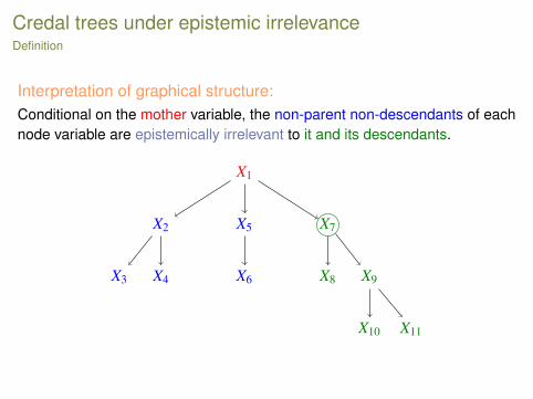
Credal trees under epistemic irrelevanceDefinition

Interpretation of graphical structure:Conditional on the mother variable, the non-parent non-descendants of eachnode variable are epistemically irrelevant to it and its descendants.

X1

X2

X3 X4

X5

X6

X7

X8 X9

X10 X11

Credal networks under epistemic irrelevanceAs an expert systemWhen the credal network is a (Markov) tree we can find the joint model fromthe local models recursively, from leaves to root.

Exact message passing algorithm

– credal tree treated as an expert system

– linear complexity in the number of nodes

Python code

– written by Filip Hermans

– testing in cooperation with Marco Zaffalon and Alessandro Antonucci

Current (toy) applications in HMMs

– character recognition [3]

– air traffic trajectory tracking and identification [1]

Example of applicationHMMs: character recognition for Dante’s Divina Commedia

Original text:

OCR output:

. . .

. . .

V

V

S1

I

S2

T

S3

A

O1

I

O2

T

O3

O

Example of applicationHMMs: character recognition for Dante’s Divina Commedia

Accuracy 93.96% (7275/7743)Accuracy (if imprecise indeterminate) 64.97% (243/374)Determinacy 95.17% (7369/7743)Set-accuracy 93.58% (350/374)Single accuracy 95.43% (7032/7369)Indeterminate output size 2.97 over 21

Table: Precise vs. imprecise HMMs. Test results obtained by twofold cross-validationon the first two chants of Dante’s Divina Commedia and n = 2. Quantification isachieved by IDM with s = 2 and modified Perks’ prior. The single-character output bythe precise model is then guaranteed to be included in the set of characters theimprecise HMM identifies.

@INPROCEEDINGScooman2011,author = De Bock, Jasper and de Cooman, Gert,title = Imprecise probability trees: Bridging two theories of imprecise probability,booktitle = ISIPTA ’09 -- Proceedings of the Sixth International Symposium on Imprecise Probability: Theories and Applications,year = 2009,editor = Coolen, Frank P. A. and de Cooman, Gert and Fetz, Thomas and Oberguggenberger, Michael,address = Innsbruck, Austria,publisher = SIPTA

Imprecise Hidden Markov Model (iHMM)

X1 X2 . . . Xk . . . Xnstates:

O1 O2 . . . Ok . . . Onoutputs:

marginal model: Q1 transition model: Qk(·|Xk−1)

emission model Sk(·|Xk)

Imprecise Hidden Markov Model (iHMM)Interpretation of the graphical structure: traditional credal networks

X1 X2 . . . Xk . . . Xn

O1 O2 . . . Ok . . . On

non-parent non-descendants node and descendants

strongly independent

Imprecise Hidden Markov Model (iHMM)Interpretation of the graphical structure: recent developments

X1 X2 . . . Xk . . . Xn

O1 O2 . . . Ok . . . On

non-parent non-descendants node and descendants

epistemically irrelevant

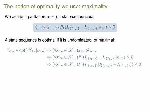
The notion of optimality we use: maximality

We define a partial order on state sequences:

x1:n x1:n⇔ P1(Ix1:n− Ix1:n|o1:n)> 0

A state sequence is optimal if it is undominated, or maximal:

x1:n ∈ opt(X1:n|o1:n)⇔ (∀x1:n ∈X1:n)x1:n 6 x1:n

⇔ (∀x1:n ∈X1:n)P1(Ix1:n− Ix1:n|o1:n)≤ 0

⇔ (∀x1:n ∈X1:n)P1(Io1:n[Ix1:n− Ix1:n])≤ 0,

P1(Io1:n[Ix1:n− Ix1:n]) can be easily determined recursively!

Aim of our EstiHMM algorithm:

Determine opt(X1:n|o1:n) exactly and efficiently.

Complexity of EstiHMM

– linear in the length of the chain n

– cubic in the number of states s

– linear in the number of maximal elements

Comparable to the Viterbi counterpart for precise HMMs.

Important conclusion:The complexity depends crucially on how the number of maximal elementsincreases with the length of the chain n

Number of maximal elementsOutput sequence (0,1,1,1,0,0) and imprecision 1%

Literature I

Enrique Miranda, A survey of the theory of coherent lower previsions.International Journal of Approximate Reasoning, 48:628–658, 2008.

Matthias Troffaes, Decision making under uncertainty using impreciseprobabilities.International Journal of Approximate Reasoning, 45:17–29, 2007.

Alessandro Antonucci, Alessio Benavoli, Marco Zaffalon, Gert deCooman, and Filip Hermans.Multiple model tracking by imprecise Markov trees.In Proceedings of the 12th International Conference on InformationFusion (Seattle, WA, USA, July 6–9, 2009), pages 1767–1774, 2009.

Gert de Cooman and Filip Hermans.Imprecise probability trees: Bridging two theories of imprecise probability.Artificial Intelligence, 172(11):1400–1427, 2008.

Literature II

Gert de Cooman, Filip Hermans, Alessandro Antonucci, and MarcoZaffalon.Epistemic irrelevance in credal networks: the case of imprecise Markovtrees.International Journal of Approximate Reasoning, 51:1029–1052, 2010.

Gert de Cooman, Filip Hermans, and Erik Quaeghebeur.Imprecise Markov chains and their limit behaviour.Probability in the Engineering and Informational Sciences,23(4):597–635, 2009.arXiv:0801.0980.

B. de Finetti.Teoria delle Probabilità.Einaudi, Turin, 1970.

Literature III

B. de Finetti.Theory of Probability: A Critical Introductory Treatment.John Wiley & Sons, Chichester, 1974–1975.English translation of [5], two volumes.

Christiaan Huygens.Van Rekeningh in Spelen van Geluck.1656–1657.Reprinted in Volume XIV of [8].

Christiaan Huygens.Œuvres complètes de Christiaan Huygens.Martinus Nijhoff, Den Haag, 1888–1950.Twenty-two volumes. Available in digitised form from the Bibliothèquenationale de France (http://gallica.bnf.fr).

G. Shafer and V. Vovk.Probability and Finance: It’s Only a Game!Wiley, New York, 2001.

Literature IV

Peter Walley.Statistical Reasoning with Imprecise Probabilities.Chapman and Hall, London, 1991.

Thomas Augustin, Frank Coolen, Gert de Cooman and Matthias Troffaes(eds.).Introduction to Imprecise Probabilities.Wiley, Chichester, mid 2012.

Also look at www.sipta.org

imprecise probabilities in stochastic processes and ...gdcooma/presentations/stochastic.pdf ·...

Documents