improved indifferentiability security bound for the jh mode
TRANSCRIPT

1
Improved Indifferentiability Security Bound for the JH Mode ∗
Dustin Moody Souradyuti Paul Daniel Smith-Tone
National Institute of National Institute of National Institute of
Standards and Technology Standards and Technology Standards and Technology
Gaithersburg, MD, USA Gaithersburg, MD, USA Gaithersburg, MD, USA
[email protected] & [email protected]
K.U.Leuven, Belgium
Abstract
The JH hash function is one of the five finalists of the ongoing NIST SHA3 hash function competition. Despite several earlier attempts, and years of analysis, the indifferentiability security bound of the JH mode has so far remained remarkably low, only up to n/3 bits [7]. Using a recent technique introduced by Moody, Paul, and Smith-Tone in [23], we improve the bound of JH to n/2 bits. We also performed experiments which verify the theoretically obtained results.
Introduction
Iterative hash functions are usually composed of two parts: (1) a basic primitive C with finite domain and range, and (2) an iterative mode of operation H to extend the domain of the hash function. We denote a hash function using the mode H and the primitive C by HC . In studying the security of a hash function, both the security of the primitive C, as well as the security of the mode of operation H need to be examined separately, since one can be attacked independently of the other.
The most popular hash mode of operation is the classical Merkle-Damgard MD mode [12, 22]. It has the desirable property that if C is collision resistant, then MDC will also be collision resistant. Many practical hash functions, such as MD4 [28], MD5 [29], SHA-0/1/2 [25, 26] use the MD mode of operation. However, several recent attacks have greatly undermined the security of any hash function based on the MD mode. Examples of such attacks include the length-extension attack, Joux’s multi-collision attack [16], the Kelsey-Kohno herding attack [17], and the Kelsey-Schneier preimage attack [18]. Each of these attacks targets the mode of operation, and they work no matter how secure the underlying primitive C is. A telltale sign of the demise of the MD mode is that none of the 64 submissions to the ongoing SHA-3 competition used the MD mode.
In search of a secure replacement for the Merkle-Damgard mode, we have broadly witnessed several stages of improvement: (1) additional postprocessing and/or counters injected into the MD mode to eliminate the length-adjustment related attacks (e.g., HAIFA [8], EMD [4], MDP [15]); (2) widening of the output length of the primitive C to eliminate Joux’s multi-collision type attacks (e.g., Widepipe-MD [20], JH [30], Grøstl [14], Sponge [5], Shabal [10], Parazoa [3]); (3) multiple applications of the primitive C on the same message-block (e.g., Doublepipe MD [20]).
Another research direction, motivated by the innovative attacks on hash modes of operation, has been the development of new security frameworks which cover the above attacks, as well as unforeseen attacks. The indifferentiability framework was introduced by Maurer et al. [21] in 2004, and was first applied to analyze
∗The extended version of this paper is available at http://www.esat.kuleuven.be/scd/person.php?persid=111
1

hash modes of operation by Coron et al. [11] in 2005. Indifferentiability measures the extent to which a hash function is behaving as a random oracle under the assumption that the underlying compression function is ideal (e.g. a random oracle, ideal permutation, or ideal cipher). A hash mode proven secure in the indifferentiability framework guarantees resistance to the attacks specifically mentioned above. Most new proposals for hash modes of operation include indifferentiability proofs of security. We note that some limitations of the indifferentiability framework have recently been discovered in [13] and [27]. Nevertheless, the framework still covers most known attack scenarios, in addition to guaranteeing resistance to many generic attacks. In this work we prove an indifferentiability bound for JH, one of the five finalists in the SHA-3 hash competition.
Figure 1: JH mode diagram: all wires are n bits.
Related Work: Since its publication, the JH mode of operation has undergone rigorous cryptanalysis. Previous indifferentiability security proofs for the JH mode were only able to obtain a bound of n/3 bits [2, 7]. In [19], it was shown that the JH mode achieves optimal collision resistance. However, improvement of the indifferentiability security of the JH mode beyond n/3 bits has remained elusive.
Our Contribution: We improve the indifferentiability security bound of the JH mode from n/3 to n/2 bits. This result guarantees the absence of generic attacks on the JH hash function with work Ω(2n/2). Furthermore, we have performed a series of experiments with the JH mode using several sets of ‘bad’ events. These bad events will be described later on. Our experiments verify the theoretically obtained results.
Notation and Convention. Throughout the paper we let n be a fixed integer. We shall use the littleendian bit-ordering system. The symbol |x| denotes the bit-length of the bit-string x, or sometimes the size
parseof the set x. Let x → x1||x2 denote parsing x into x1 and x2 such that |x1| = n and |x2| = |x|− n. Let SX
denote the sample space of the discrete random variable X. The relation A ∼ B is satisfied if and only if n n Pr A = X = Pr B = X for all X ∈ S, where S = SA = SB . Other notation which we will use is included in Table 1.
Table 1: Notation
AB Algorithm A with oracle access to B Dom(T ) The set of indices I in table T such that T [i] =⊥ ∀i ∈ I
ab a||b [x, y] The set of integers between (and including) x and y a[x, y] The bit-string between the xth and yth bit-positions of a U [0, N ] The uniform distribution over the integers between 0 and N
2

1.1 Description of the JH Mode
JH(M) pad
01. M → m1m2 . . .mk−1mk; b02. y0 = IV , y = IV b;0
03. for(i = 11, 2, . . . k) Figure 3: Indifferentiability frameyiy
b = π yi−1||(yb ⊕ mi) ⊕ mi||0; work for a hash function based on an i i−1
04. return yk; ideal permutation. An arrow indicates the direction in which a query
Figure 2: Pseudocode for the JH hash function is submitted.
Suppose n ≥ 1. Let π : {0, 1}2n → {0, 1}2n be a 2n-bit ideal permutation used to build the JH hash function JHπ : {0, 1}∗ → {0, 1}n . The diagram and the description of the JH transform are given in Figures 1
pad iand 2. The semantics for the notation M → m1 · · · mk−1mk is as follows: Using an injective function
pad : {0, 1}∗ → ∪i≥1{0, 1}ni , M is mapped into a string m1 · · · mk−1mk such that k ≥ |M | +1, |mi| = n for n
1 ≤ i ≤ k. In addition to the injectivity of pad(·), we will also require that there exists a function dePad(·) that can efficiently compute M , given pad(M). Formally, the function dePad : ∪i≥1 {0, 1}in → {λ} ∪ {0, 1}∗
computes dePad(pad(M)) = M , for all M ∈ {0, 1}∗, and otherwise dePad(·) returns λ. We note that the padding rules of all practical hash functions have the above properties.
1.2 Preliminaries: Introduction to the Indifferentiability Framework
We begin with the definition of a random oracle. This useful object will be used frequently in the subsequent discussion.
Definition 1.1 (Random oracle) A random oracle is a function RO : X → Y chosen uniformly at random from the set of all |Y ||X| functions that map X → Y . In other words, a function RO : X → Y is a random oracle if and only if, for each x ∈ X, the value of RO(x) is chosen uniformly at random from Y .
Corollary 1.2 If a function RO : X → Y is a random oracle, then n 1 Pr RO(x) = y|RO(x1) = y1, RO(x2) = y2, . . . , RO(xq) = yq =
|Y |
where x /∈ {x1, x2, . . . , xq}, y ∈ Y and q ∈ Z.
Next we introduce the indifferentiability framework and briefly discuss its significance. The definition we give is a slightly modified version of the original definition provided in [11, 21].
Definition 1.3 (Indifferentiability framework) [11] An interactive Turing machine (ITM) T with oracle access to an ideal primitive F is said to be (tA, tS , q, ε)-indifferentiable from an ideal primitive G if there exists a simulator S such that, for any distinguisher A, the following equation is satisfied:
|Pr[AT,F = 1] − Pr[AG,S = 1]| ≤ ε.
The simulator S is an ITM which has oracle access to G and runs in time at most tS . The distinguisher A runs in time at most tA. The number of queries used by A is at most q. Here ε is a negligible function in the security parameter of T .
3
2
G,S G,SWe define Adv = maxA |Pr[AT,F = 1]−Pr[AG,S = 1]|, so that by definition Adv ≤ ε. The significance T,F T,F of the framework is as follows. Suppose, an ideal primitive G (e.g. a variable-input-length random oracle) is indifferentiable from an algorithm T based on another ideal primitive F (e.g. a fixed-input-length random oracle). In such a case, any cryptographic system P based on G is as secure as P based on T F (i.e., G replaces T F in P). For a more detailed explanation, we refer the reader to [21].
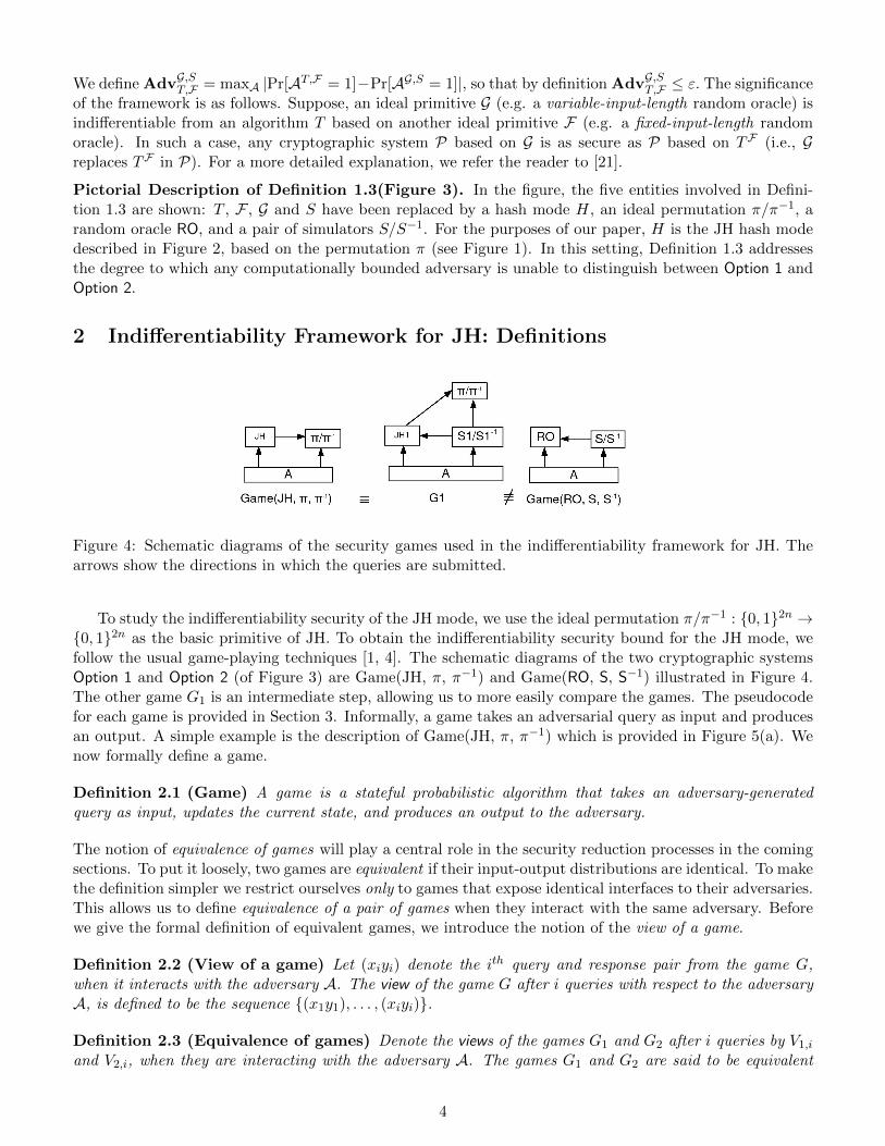
Pictorial Description of Definition 1.3(Figure 3). In the figure, the five entities involved in Definition 1.3 are shown: T , F , G and S have been replaced by a hash mode H, an ideal permutation π/π−1, a random oracle RO, and a pair of simulators S/S−1 . For the purposes of our paper, H is the JH hash mode described in Figure 2, based on the permutation π (see Figure 1). In this setting, Definition 1.3 addresses the degree to which any computationally bounded adversary is unable to distinguish between Option 1 and Option 2.
Indifferentiability Framework for JH: Definitions
Figure 4: Schematic diagrams of the security games used in the indifferentiability framework for JH. The arrows show the directions in which the queries are submitted.
To study the indifferentiability security of the JH mode, we use the ideal permutation π/π−1 : {0, 1}2n → {0, 1}2n as the basic primitive of JH. To obtain the indifferentiability security bound for the JH mode, we follow the usual game-playing techniques [1, 4]. The schematic diagrams of the two cryptographic systems Option 1 and Option 2 (of Figure 3) are Game(JH, π, π−1) and Game(RO, S, S−1) illustrated in Figure 4. The other game G1 is an intermediate step, allowing us to more easily compare the games. The pseudocode for each game is provided in Section 3. Informally, a game takes an adversarial query as input and produces an output. A simple example is the description of Game(JH, π, π−1) which is provided in Figure 5(a). We now formally define a game.
Definition 2.1 (Game) A game is a stateful probabilistic algorithm that takes an adversary-generated query as input, updates the current state, and produces an output to the adversary.
The notion of equivalence of games will play a central role in the security reduction processes in the coming sections. To put it loosely, two games are equivalent if their input-output distributions are identical. To make the definition simpler we restrict ourselves only to games that expose identical interfaces to their adversaries. This allows us to define equivalence of a pair of games when they interact with the same adversary. Before we give the formal definition of equivalent games, we introduce the notion of the view of a game.
Definition 2.2 (View of a game) Let (xiyi) denote the ith query and response pair from the game G, when it interacts with the adversary A. The view of the game G after i queries with respect to the adversary A, is defined to be the sequence {(x1y1), . . . , (xiyi)}.
Definition 2.3 (Equivalence of games) Denote the views of the games G1 and G2 after i queries by V1,i
and V2,i, when they are interacting with the adversary A. The games G1 and G2 are said to be equivalent
4

3
with respect to the adversary A if and only if V1,i ∼ V2,i, for all i > 0. Equivalence between the games G1 A
and G2 with respect to the adversary A is denoted by G1 ≡ G2, or simply G1 ≡ G2, when the adversary is clear from the context.
Next we state an important lemma relating the equivalence of games and the adversarial outputs. nnA AG1 AG2⇒ 1 = Pr ≡ G2 then Pr ⇒ 1 . The probabilities are taken over all coin tosses Lemma 2.4 If G1
in the games and the adversary.
Proof. The result follows immediately from Definition 2.3. D
Roadmap. From Section 1.2, we have
Pr . RO,S/S−1
In the following sections we shall estimate Adv using the following approach: JH,π/π−1
• In Section 3 and 4 we describe the security games presented in Figure 4; an important part of the description is designing a simulator-pair S/S−1 for the indifferentiability framework for JH, and computing an upper bound of O(σ5) on the running time of the simulator-pair, where σ is the maximum
.
n nRO,S/S−1
AGame(JH, π, π−1) ⇒ 1 AGame(RO, S, S−1) ⇒ 1− PrAdv = max JH,π/π−1 A
nnnumber of invocations to the ideal permutation π/π−1 . Additionally, we shall show that Game(JH, AGame(JH, π, π−1) ⇒ 1π, π−1)≡ G1, which implies by Lemma 2.4, Pr AG1= Pr ⇒ 1 . This, in turn,
implies:
RO,S/S−1 Pr
AG1 ⇒ 1 − Pr
n n AGame(RO, S, S−1) ⇒ 1AG1 ⇒ 1 − PrAdv = max
JH,π/π−1 A
• Then in Section 5 we shall show n AGame(RO, S, S−1) ⇒ 1
= O
σ2
.max Pr n
A 2n
The n/2 bit indifferentiability security bound follows from this last equation.
Description of the Security Games for JH
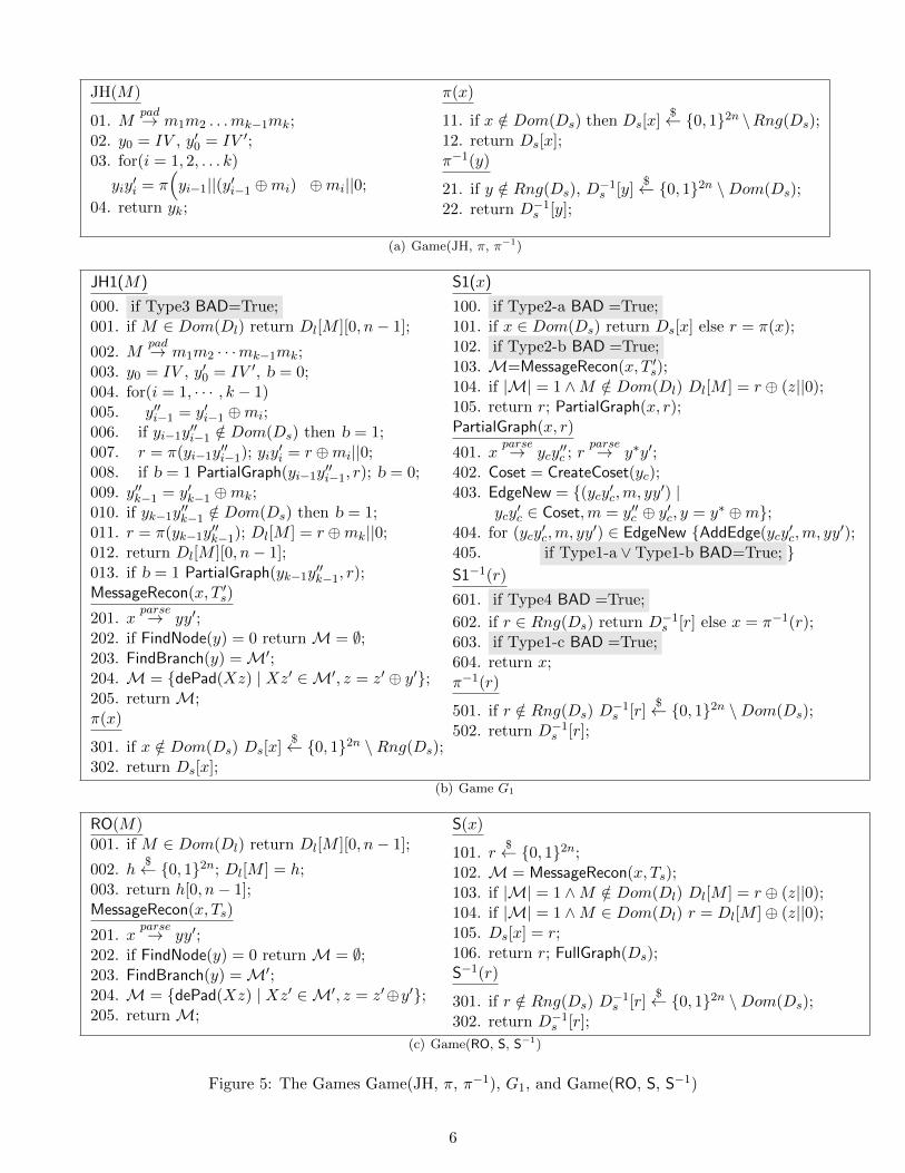
In this section, we elaborate on the games Game(JH, π, π−1), G1, and Game(RO, S, S−1) that are schematically presented in Figure 4. The pseudocode for all the games is given in Figure 5. The functions JH, JH1, and RO are mappings from {0, 1}∗ → {0, 1}n . We use the generic term long oracle (or l-oracle) to identify any of them and call any query submitted to a long oracle an l-query. Also, π, and S1 are permutations on {0, 1}2n . The oracle S is a mapping from {0, 1}2n → {0, 1}2n . These three oracles are called forward short oracles (or forward s-oracles). The corresponding queries are called forward s-queries. Similarly, π−1 , S1−1 , and S−1 are also permutations on {0, 1}2n which are called reverse short oracles (or reverse s-oracles). We assume that identical queries are not submitted more than once. The games will use several global and local variables. The tables Dl, Ds, and all local variables are initialized with ⊥. The graph Ts initially contains only the root node (IV, IV b). The local variables are re-initialized every new invocation of the game, while the global data-structures maintain their states across the queries.
Description of Game(JH, π, π−1) (Figure 5(a)). The game Game(JH, π, π−1) implements three functions: the l-oracle JHπ, the forward s-oracle π, and the reverse oracle π−1 . The definition of the function JHπ was given in Section 2. The ideal permutation π/π−1 has been implemented through lazy sampling. The query-response pairs for π/π−1 are stored in the table Ds.
5
JH(M) π(x)
01. M pad→ m1m2 . . . mk−1mk;
02. y0 = IV , yb 0 = IV b; 03. for(i = 1, 2, . . . k)1
yiyb i = π yi−1||(yb i−1 ⊕ mi)
04. return yk; ⊕ mi||0;
11. if x /∈ Dom(Ds) then Ds[x] $← {0, 1}2n \ Rng(Ds);
12. return Ds[x]; π−1(y)
21. if y /∈ Rng(Ds), D−1 s [y]
$← {0, 1}2n \ Dom(Ds); 22. return D−1
s [y];
(a) Game(JH, π, π−1)
JH1(M) S1(x)
000. if Type3 BAD=True; 100. if Type2-a BAD =True; 001. if M ∈ Dom(Dl) return Dl[M ][0, n − 1]; 101. if x ∈ Dom(Ds) return Ds[x] else r = π(x);
pad 102. if Type2-b BAD =True; 002. M → m1m2 · · · mk−1mk; b 103. M=MessageRecon(x, T b);003. y0 = IV , y = IV b , b = 0; s0
004. for(i = 1, · · · , k − 1) 104. if |M| = 1 ∧ M /∈ Dom(Dl) Dl[M ] = r ⊕ (z||0); bb b 105. return r; PartialGraph(x, r);005. y = y ⊕ mi;i−1 i−1
bb PartialGraph(x, r)006. if yi−1yi−1 ∈/ Dom(Ds) then b = 1; parse parsebb b bb ∗ b007. r = π(yi−1y ); yiy = r ⊕ mi||0; 401. x → ycy ; r → y y ;i−1 i c
bb008. if b = 1 PartialGraph(yi−1yi−1, r); b = 0; 402. Coset = CreateCoset(yc); bb b b009. y = y ⊕ mk; 403. EdgeNew = {(ycy ,m, yyb) |k−1 k−1 c
bb b bb b010. if yk−1y ∈/ Dom(Ds) then b = 1; ycy ∈ Coset,m = y ⊕ y , y = y ∗ ⊕ m};k−1 c c cbb b b011. r = π(yk−1y ); Dl[M ] = r ⊕ mk||0; 404. for (ycy ,m, yyb) ∈ EdgeNew {AddEdge(ycy ,m, yyb);k−1 c c
012. return Dl[M ][0, n − 1]; 405. if Type1-a ∨ Type1-b BAD=True; }bb013. if b = 1 PartialGraph(yk−1yk−1, r); S1−1(r)
MessageRecon(x, T b)s 601. if Type4 BAD =True; parse b201. x → yy ; 602. if r ∈ Rng(Ds) return D−1[r] else x = π−1(r);s
202. if FindNode(y) = 0 return M = ∅; 603. if Type1-c BAD =True; 203. FindBranch(y) = Mb; 604. return x; 204. M = {dePad(Xz) | Xzb ∈Mb, z = zb ⊕ yb}; π−1(r) 205. return M; $
) D−1501. if r /∈ Rng(Ds [r] ← {0, 1}2n \ Dom(Ds);sπ(x) 502. return D−1[r];
$ s 301. if x /∈ Dom(Ds) Ds[x] ← {0, 1}2n \ Rng(Ds); 302. return Ds[x];
(b) Game G1
RO(M) S(x) 001. if M ∈ Dom(Dl) return Dl[M ][0, n − 1]; $
101. r ← {0, 1}2n;$
002. h ← {0, 1}2n; Dl[M ] = h; 102. M = MessageRecon(x, Ts); 003. return h[0, n − 1]; 103. if |M| = 1 ∧ M /∈ Dom(Dl) Dl[M ] = r ⊕ (z||0); MessageRecon(x, Ts) 104. if |M| = 1 ∧ M ∈ Dom(Dl) r = Dl[M ] ⊕ (z||0);
parse201. x → yyb; 105. Ds[x] = r; 202. if FindNode(y) = 0 return M = ∅; 106. return r; FullGraph(Ds);
S−1(r)203. FindBranch(y) = Mb; $
) D−1204. M = {dePad(Xz) | Xzb ∈Mb, z = zb ⊕yb}; 301. if r /∈ Rng(Ds [r] ← {0, 1}2n \ Dom(Ds);s 205. return M; 302. return D−1[r];s
(c) Game(RO, S, S−1)
Figure 5: The Games Game(JH, π, π−1), G1, and Game(RO, S, S−1)
6
Description of Game(RO, S, S−1) (Figure 5(c)). In this game, the pair of s-oracles S/S−1 is the simulator pair for the indifferentiability framework of JH. The l-oracle of this game implements the random oracle RO. Construction of an effective simulator pair is perhaps the most important part in the analysis of the indifferentiability security for a hash mode of operation. The purpose of the simulator pair S/S−1 is two-fold: (1) to output values which are indistinguishable from the output of the ideal permutation π/π−1, and (2) to respond in such a way that JHπ(M) and RO(M) are identically distributed. It will easily follow that as long as the simulator pair S/S−1 is able to output values satisfying the above conditions, no adversary can distinguish between Game(JH, π, π−1) and Game(RO, S, S−1).
Our design strategy for S/S−1 is fairly intuitive and simple. However, before jumping into a detailed description, we define the data structures and the subroutines. The game uses three global data structures: the table Ds, which stores all s-queries and their responses, the table Dl, which stores all l-queries and their responses, and finally a specially designed directed graph Ts.
• Subroutine FullGraph(): This subroutine updates the directed graph Ts using the elements stored in Ds. The graph Ts is built in such a way that each path originating from the root-node (IV, IV b)
padrepresents the execution of JH(·) on a prefix of some message. For instance, suppose M → m1m2M
b . m1 m2b bThen the path IV IV b → y1y → y2y represents the first two-block execution of JH(M) where, 1 2
b b by1y = π(IV ||IV ⊕ m1) ⊕ m1||0 and y2y = π(y1||y1 ⊕ m2) ⊕ m2||0. See Figure 6 for a pictorial 1 2 description. Additionally and more importantly, the graph Ts contains all possible paths derived from the elements in Ds; hence the name FullGraph.
• Subroutine MessageRecon(x, Ts): The purpose of this subroutine is to reconstruct all messages M , such that JHπ(M) can be computed using the elements in Ds, and π(x). As the final input to π in JHπ(M) is x, we see JHπ(M) = π(x)[0, n − 1] ⊕ mk, where mk is the final block of the reconstructed message M .
In order to find the messages, the subroutine FindNode(y = x[0, n−1]) first checks whether there exists a node in the graph Ts with left-coordinate y (line 202). If present, then the subroutine FindBranch(y) collects all paths from the root node (IV, IV b) to these nodes of the form yzb, and returns a set M. The set M contains the sequences of arrows on the paths found, each concatenated with z = zb ⊕x[n, 2n−1] (lines 203 and 204). If there are no nodes with left coordinate y, then the empty set is returned (line 202).
On a new forward s-query x, the simulator S assigns a uniformly sampled 2n-bit value to r (line 101). The subroutine MessageRecon(x, Ts) is then invoked, returning a set of messages M (line 102). If the size of
padM is 1 and M (such that M → Xz ∈M) is not an old l-query, then Dl[M ] is assigned the value of x (line 103). If M is an old l-query, then r is assigned the value of Dl[M ] (line 104). In lines 105 and 106 the table Ds is updated and the value of r is returned. Finally, the graph Ts is updated. We will see very shortly that the worst-case running time of S on the ith query is O(i4).
On a new reverse s-query r, S−1 returns a uniformly sampled 2n-bit value chosen from the set {0, 1}2n \ Dom(Ds) (lines 301 and 302).
For a new l-query M , the random oracle RO first checks whether M has already been reconstructed using forward s-queries. In such a case, M already belongs to Dom(Dl) and RO returns the least-significant n bits of Dl[M ], i.e. Dl[M ][0, n − 1] (line 001). Otherwise, the value for Dl[M ] is assigned a uniformly sampled 2n-bit value (line 002), and the least-significant n bits are returned (line 003).
Time Complexity of the Simulator S Since there are i queries after i rounds, the maximum number of nodes in Ts is i2 . Therefore, to construct the fullgraph at ith round, the amount of time required is O(i4). Now if the adversary submits σ queries, then the time complexity is O(σ5). Since the fullgraph construction dominates the simulator time, the simulator time complexity is also O(σ5).
Description of G1 (Fig. 5(b)). The description of the game G1 might look a bit artificial in the sense
7

Figure 6: All wires are n bits. (i) The directed graph Ts is updated by the subroutines FullGraph or b b bPartialGraph (see Sect. 3). Example: The edge (y1y1,m2, y2y2) is composed of the head node y1y1, the arrow
b b bm2, and the tail node y2y2. (ii) Generation of the edge (y1y1,m2, y2y2) of Ts using π; the shaded rectangle is viewed as the compression function of JH with y1y1
b m2 being the input and y2y2 b as the output.
that it was constructed as a hybridization of the games Game(JH, π, π−1) and Game(RO, S, S−1). The purpose of this game is to be a transition point from Game(JH, π, π−1) to Game(RO, S, S−1) so that their difference in execution can be easily examined. As in Game(RO, S, S−1), the global variables are the tables Ds and Dl, and the graph Ts.
In our initial description of this game, we omit the statements where the variable BAD is set (lines 000, 100, 102, 405, 601, and 603), since they do not impact the output and the global data structures. The variable BAD is set when certain events occur in the global data structures. Those events will be discussed, n n
AG1 ARO,S,S−1 when we compute Pr ⇒ 1 −Pr ⇒ 1 in Section 5. The subroutines in this game are similar to the ones for Game(RO, S, S−1):
• Subroutine PartialGraph(x, r): Like FullGraph, this subroutine also builds the graph Ts in such a way that each directed path originating from the root-node (IV, IV b) represents the execution of JH(·) on a prefix of some message (depicted in Figure 6). However, there are important differences. Rather than building all possible paths using the new pair (x, r) and the old pairs in Ds, PartialGraph augments Ts
in at most one phase; hence its name.
PartialGraph invokes the subroutine CreateCoset(yc = x[0, n − 1]), which returns a set Coset containing all nodes in Ts, whose left-coordinate is yc (lines 401 and 402). The size of Coset determines the number of nodes to be added to Ts in the the current iteration. Using the members of Coset and the new pair (x, r), new edges are constructed, stored in EdgeNew, and added to Ts using the subroutine AddEdge.
• Subroutine MessageRecon(x, T b): This subroutine is virtually the same as described in game Game(RO,s
S, S−1). The only difference is that instead of the graph Ts, the second argument to this subroutine is T b, which is the maximally connected subgraph of Ts with root-node (IV, IV b), generated by a part of s
the table Ds which contains only the forward s-queries and their responses. Note that in addition to forward s-query/responses, Ds may also contains reverse s-query/responses, as well as π-query/response pairs generated during the execution of l-queries. This is a significant difference between this game and Game(RO, S, S−1), which does not have any π-queries arising from the processing of an l-query. This difference will be quantified in Section 5.
Given a forward s-query x, if x ∈ Dom(Ds) then Ds[x] is returned by S1. Otherwise, π(x) is computed (line 101). We see the ideal permutation π is implemented through lazy sampling (lines 301 and 302). The subroutine MessageRecon is called with input (x, T b), which returns a set of reconstructed messages M (lines
pad103). If the size of M is 1, and if the M is not a previous l-query (such that M → Xz ∈M), then Dl[M ] is assigned the value of π(x) ⊕ z||0 (line 104). After finally returning r (line 105), the subroutine PartialGraph is called on the input (x, r) to update the existing graph Ts.
8

4
The reverse s-oracle S1−1 is identical to the oracle S−1 of Game(RO, S, S−1). If an l-query M has already been reconstructed by S1 on some previous forward s-query, then Dl[M ][0, n−
1] is returned (line 001). Otherwise, (lines 002-012) JH1 mimics JH. It also updates the graph Ts (lines 008 and 013), whenever a new intermediate input is generated (lines 006 and 010). Afterwards, the value of Dl[M ] is assigned to be r ⊕ mk||0 (line 011). Finally, Dl[M ][0, n − 1] is returned (line 012). The graph Ts is also updated, if necessary (line 013).
Remark 1 The difference in how the subroutines FullGraph and PartialGraph construct the directed graph Ts forms the first non-trivial step towards improving the bound for the indifferentiability security of JH. The PartialGraph augments Ts in at most one phase every invocation. It is easy to see that the graph Ts arising from PartialGraph is a connected subgraph of the Ts constructed by the FullGraph. We will show that if the events in lines 000, 001, 100, 102, 405, 601, and 603 do not occur, then both subroutines build identical graphs. As a consequence, the probability of occurrence of these ”BAD” events constitutes a significant fraction of JH’s overall indifferentiability bound of O(σ2n
2 ). It seems possible that if PartialGraph were to
augment Ts in more than one phase, the indifferentiability bound could be further improved. However, in this case, the determination of a non-trivial upper-bound on the probability of the BAD events seems to be hard. For more details, see the extended version of this paper.
With the above description of the games at our disposal, we are well equipped to state and prove an easy, but important, result.
Proposition 3.1 For any distinguishing adversary A, Game(RO, S, S−1)≡ G1.
Proof. From the description of S1, and S1−1, we observe that, for all x ∈ {0, 1}2n , S1(x) = π(x), and S1−1(x) = π−1(x) (lines 101, and 602). Likewise, from the descriptions of JH1 and JH, for all M ∈ {0, 1}∗ , JH1(M) =JH(M). D
The events Type1, Type2, Type3, and Type4 mentioned in Figure 5(b) are still undefined. These events are used to distinguish game G1 from game Game(RO, S, S−1). We describe them in the next section.
Definition of the events BADi, and GOODi
For the remainder of the paper, by a query we will mean either a message-block in an l-query, or a forward or reverse s-query. With this convention, we see that prior to the ith query, the sum of the s-queries and message-blocks contained in l-queries is thus i − 1. The purpose of this section is to concretely define the Type1, Type2, Type3 and Type4 events mentioned in lines 405, 603, 001, 100, 102, 000, and 601 of game G1 (Figure 5(b)). Before doing so, we define a few additional events that can be defined using the Type1, Type2, Type3, and Type4 events.
• Let the symbol BADi denote the event when the variable BAD is set (in lines 405, 603, 001, 100, 102, 000, and 601) on the ith query in game G1. In other words, BADi occurs when one or more of Type1, Type2, Type3, or Type4 events occur on the ith query in game G1.
• The symbol GOODi denotes ¬ ∨ij=1 BADib for all i > 0.
• We use the symbol GOOD0 to denote the event when no queries have been submitted in game G1.
From a high level, the intuition behind the construction of the BADi events in the game G1 is rather straightforward. We make sure that if BADi does not occur, and if GOODi−1 did occur, then the views of G1 and Game(RO, S, S−1) (up to the ith query) are identically distributed for any attacker A. Hence, the BADi
events will establish the following lemma.
9
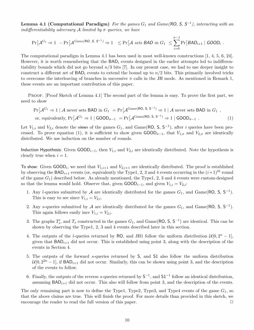
Lemma 4.1 (Computational Paradigm) For the games G1 and Game(RO, S, S−1), interacting with an indifferentiability adversary A limited by σ queries, we have
σ−1n n n a n AG1 AGame(RO, S, S−1) ⇒ 1Pr ⇒ 1 − Pr ≤ Pr A sets BAD in G1 ≤ Pr BADi+1 | GOODi .
i=0
The computational paradigm in Lemma 4.1 has been used in most well-known constructions [1, 4, 5, 6, 24]. However, it is worth remembering that the BADi events designed in the earlier attempts led to indifferentiability bounds which did not go beyond n/3 bits [7]. In our present case, we had to use deeper insight to construct a different set of BADi events to extend the bound up to n/2 bits. This primarily involved tricks to overcome the interleaving of branches in successive π calls in the JH mode. As mentioned in Remark 1, these events are an important contribution of this paper.
Proof. [Proof Sketch of Lemma 4.1] The second part of the lemma is easy. To prove the first part, we need to show n n
AG1Pr ⇒ 1 | A never sets BAD in G1 = Pr AGame(RO, S, S−1) ⇒ 1 | A never sets BAD in G1 , n n or, equivalently, Pr AG1 ⇒ 1 | GOODσ−1 = Pr AGame(RO, S, S−1) ⇒ 1 | GOODσ−1 . (1)
Let V1,i and V2,i denote the views of the games G1, and Game(RO, S, S−1), after i queries have been processed. To prove equation (1), it is sufficient to show given GOODσ−1, that V1,σ and V2,σ are identically distributed. We use induction on the number of rounds.
Induction Hypothesis: Given GOODi−1, then V1,i and V2,i are identically distributed. Note the hypothesis is clearly true when i = 1.
To show: Given GOODi, we need that V1,i+1 and V2,i+1 are identically distributed. The proof is established by observing the BADi+1 events (or, equivalently the Type1, 2, 3 and 4 events occurring in the (i+1)th round of the game G1) described below. As already mentioned, the Type1, 2, 3 and 4 events were custom-designed so that the lemma would hold. Observe that, given GOODi−1, and given V1,i = V2,i:
1. Any l-queries submitted by A are identically distributed for the games G1, and Game(RO, S, S−1). This is easy to see since V1,i = V2,i.
2. Any s-queries submitted by A are identically distributed for the games G1, and Game(RO, S, S−1). This again follows easily ince V1,i = V2,i.
3. The graphs T b, and Ts constructed in the games G1, and Game(RO, S, S−1) are identical. This can be s
shown by observing the Type1, 2, 3 and 4 events described later in this section.
4. The outputs of the l-queries returned by RO, and JH1 follow the uniform distribution U [0, 2n − 1], given that BADi+1 did not occur. This is established using point 3, along with the description of the events in Section 4.
5. The outputs of the forward s-queries returned by S, and S1 also follow the uniform distribution U [0, 22n − 1], if BADi+1 did not occur. Similarly, this can be shown using point 3, and the description of the events to follow.
6. Finally, the outputs of the reverse s-queries returned by S−1, and S1−1 follow an identical distribution, assuming BADi+1 did not occur. This also will follow from point 3, and the description of the events.
The only remaining part is now to define the Type1, Type2, Type3, and Type4 events of the game G1, so that the above claims are true. This will finish the proof. For more details than provided in this sketch, we encourage the reader to read the full version of this paper. D
10

c
4.1 Type1 Event
Type1 events occur in lines 405, and 603 in Figure 5(b). We divide them into three subcases. Suppose b(ycy ,m, yyb) is a new edge generated from a new query/response (x, r) (lines 401 through 404).
• Type1-a event (Figure 7(Type1-a)): This event occurs if y collides with the left-coordinate of a node already in Ts.
• Type1-b event (Figure 7(Type1-b)): This event occurs if y collides with the least-significant n bits of a query already in Ds.
• Type1-c event (Figure 7(Type1-c)): This event occurs if the least-significant n bits of output of a reverse s-query match with the left-coordinate of a node already in Ts.
New
y* y’
=
y
y’c
yc
Node-collision
(n bits)
Old
m
New
y* y’
=
y
y’c
yc
m
old
Old
=
y
New
Forward-query-collision
(n bits)Reverse-query-collision
(n bits)
Type1-a Type1-b Type1-c
y’’
Figure 7: Type1 events when BAD is set in lines 405 and 603 of game G1 (Figure 5(b)). All arrows are n bits. A red arrow denotes new n bits of output from the ideal permutation π/π−1 . The symbol “=” denotes n-bit equality.
4.2 Type2 Event
This event is mentioned in lines 100 and 102 of game G1. In order to define Type2 events, we need to classify all old query-response pairs to the oracles π/π−1 stored in Ds, according to their known and unknown parts. The known part of a query-response pair is the part which is present in the view of the game G1, while the unknown part is not present. We note that there are seven types of such pairs. The first six types are generated due to the intermediate π calls made during l-queries. The type Q7 queries are the old s-queries. See Figure 8(a).
A Type2-a event occurs, if the output of a forward s-query is one of the types Q1, Q2, Q3, Q4, Q5, and Q6, and the output can be distinguished from the uniform distribution. The Type2-b event occurs, if the output of a new forward s-query can be distinguished from the uniform distribution.
11

Q5Q1 Q4Q2 Q3 Q6 Q7
New
~U[0,2
n-1]
Type2-a
New
~U[0,2
2n-1]
~U[0,2
2n-1]
Type2-b
(a) Seven types of input-output pairs for π/π−1-query; Type2 events for which BAD is set in lines 100 and 102 of game G1.
A p
ath
on
Ts r
ep
rese
ntin
g a
n l-q
ue
ry
(ii)
~U[0,2
2n-1]
(iii)
Q4/Q4/Q5
=
Q1/Q2/Q3
(i)
Q7
Q7
Q5Q1 Q4Q2 Q3 Q6
(b) Type3 events for which BAD is set in line 000 of game G1.
Q5Q1 Q4Q2 Q3 Q6 Q7
New
==
(c) Type4 events for which BAD is set in line 601 of game G1.
Figure 8: Pictorial description of Type2, Type3, and Type4 events of the game G1 (Figure 5(b)). Green circles and green arrows denote n bits present in the view of the game. Red circles denote n bits not present in the view. A red arrow denotes new n bits of output from the ideal permutation π/π−1 . The symbols “=”, and “==” denote n-bit and 2n-bit equality respectively.
12
4.3 Type3 Event
This event is mentioned in line 000 of game G1. A Type3 event occurs when an l-query M is submitted in the game G1, and JHπ(M) can be computed from the entries already stored in Ds. We divide this case into three subcases, according to the final π-query. The first subase is when the final π-query is of type Q1, or Q2, or Q3. A simple observation shows that this case cannot happen, since this would imply a left-coordinate-collision in Ts, forbidden by the occurrence of GOODi. The second subcase is if the final π-query is of type Q4, or Q5, or Q6. The Type3 event occurs, if an adversary distinguishes the 2n bits of final output from the uniform distribution U [22n − 1]. Finally, the third subcase is when the final π-query is of type Q7. In this situation, the Type3 event occurs if JHπ(M) can be computed on an existing path of the graph Ts, and if the path has an π-query/response whose type is one of Q1, Q2, Q3, Q4, Q5 and Q6. See Figure 8(b) for a graphical description.
4.4 Type4 Event
The final event is mentioned in line 601 of game G1. A Type4 event occurs, if the input of a fresh reverse s-query matches with a query of type Q1, Q2, Q3, Q4, Q5, or Q6. See Figure 8(c). n n
AG1 ARO,S ⇒ 15 Estimation of Pr ⇒ 1 − Pr
We individually compute the probabilities of each of the events described in Section 4. We need the help of the following lemma to provide a rigorous analysis for the upper-bounds we compute in this section.
Lemma 5.1 (Correction Factor) If the advantage of an indifferentiable adversary A for the games G1
and Game(RO, S, S−1), limited by σ queries, is bounded by ε, which is a negligible function in the security parameter n, then n 1
Pr GOODi ≥ C
for some constant C > 0, for all 0 ≤ i ≤ σ − 1, and for all n > 0. n Proof. Since ε < 1 for all n > 0, Pr A sets BAD in G1 ≤ ε ≤ 1 − C
1 for some constant C > 0, and for all n n > 0. Also note that Pr GOODi is a decreasing function in i. Hence the result. D
The Type1-a event guarantees that that if Ts is GOODi, then it has O(i) nodes, thus from Figure 7, we obtain,
Pr Type1i+1 | GOODi ≤ 3i/2n , 1 i = O . (2)
2n
Using the definition of Type2 events in Section 4, and their representation in Figure 8(a), it is easy to deduce: 1n i
Pr Type2i+1 | GOODi = O . 2n
Similarly, with the definition of Type3 events in Section 4, and Figure 8(b), we find: 1n 1 Pr Type3i+1 | GOODi = O .
2n
Finally, using the definition of Type4 events, it follows that: 1n i Pr Type4i+1 | GOODi = O .
2n
13
6
We conclude with the following inequality which holds for 0 ≤ i ≤ σ −1. By the upper-bounds computed above, we obtain n n n
Pr BADi+1 | GOODi ≤ Pr Type1i+1 | GOODi + Pr Type2i+1 | GOODi n n + Pr Type3i+1 | GOODi + Pr Type4i+1 | GOODi 1 i = O . (3)
2n
Therefore, by Lemma 4.1, for all A,
σ−1an n n Pr AG1 ⇒ 1 − Pr AGame(RO, S, S−1) ⇒ 1 ≤ Pr BADi+1 | GOODi
i=0
σ−1 1a i ≤ O 2n
i=0 1σ2
= O . (4)2n
This last equation (4) yields the bound of n/2.
Experimental Results
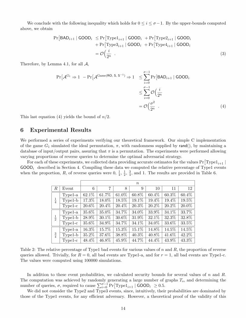
We performed a series of experiments verifying our theoretical framework. Our simple C implementation of the game G1 simulated the ideal permutation, π, with randomness supplied by rand(), by maintaining a database of input/output pairs, assuring that π is a permutation. The experiments were performed allowing varying proportions of reverse queries to determine the optimal adversarial strategy. n
For each of these experiments, we collected data providing accurate estimates for the values Pr Type1i+1 |GOODi described in Section 4. Compiling these data we computed the relative percentage of Type1 events
1 3when the proportion, R, of reverse queries were 0, 14 , 2 , , and 1. The results are provided in Table 6. 4
n R Event 6 7 8 9 10 11 12
1 4
Type1-a 62.1% 61.7% 61.0% 60.8% 60.4% 60.3% 60.4% Type1-b 17.3% 18.0% 18.5% 19.1% 19.4% 19.4% 19.5% Type1-c 20.6% 20.4% 20.4% 20.3% 20.2% 20.2% 20.0%
1 2
Type1-a 35.6% 35.0% 34.7% 34.0% 33.9% 34.1% 33.7% Type1-b 28.9% 30.1% 30.6% 31.9% 32.1% 32.3% 32.8% Type1-c 35.6% 34.9% 34.7% 34.1% 34.0% 33.6% 33.5%
3 4
Type1-a 16.3% 15.7% 15.3% 15.1% 14.8% 14.5% 14.5% Type1-b 35.2% 37.6% 38.8% 40.3% 40.8% 41.6% 42.2% Type1-c 48.4% 46.8% 45.9% 44.7% 44.4% 43.9% 43.3%
Table 2: The relative percentage of Type1 bad events for various values of n and R, the proportion of reverse queries allowed. Trivially, for R = 0, all bad events are Type1-a, and for r = 1, all bad events are Type1-c. The values were computed using 100000 simulations.
In addition to these event probabilities, we calculated security bounds for several values of n and R. The computation was achieved by randomly generating a large number of graphs Ts, and determining the n number of queries, σ, required to cause
σ−1 Pr Type1i+1 | GOODi ≥ 0.5.i=0 We did not consider the Type2 and Type3 events, since, intuitively, their probabilities are dominated by
those of the Type1 events, for any efficient adversary. However, a theoretical proof of the validity of this
14

7
assumption is still an open problem. We found that choosing the values at which to place the first query uniformly at random from among all possible maximal left-cosets was the most advantageous strategy for an adversary.
The results of the experiments following this method are summarized in Figure 9. The data supports the theoretically obtained bound of σ = Ω(2n/2) (see Equation 4). Some of the values in the graph are slightly lower than 1/2, due to the effect of constants. We expect the data to asymptotically approach 1/2.
Figure 9: Plot of experimental data of value of n versus the normalized logarithm of σ, log2(σ)/n, for the game G1 with various values of r, the proportion of reverse queries allowed.
The data indicates that the optimal adversarial strategy for game G1 is to disallow reverse queries. For each fixed R < 1, however, we observe that the data asymptotically approaches 1/2. Although it is the case that for R = 1, σ has an expected value of 2n−1, we conjecture that for any fixed value of R < 1, σ = Θ(2n/2).
Conclusion
In this paper we improved the indifferentiability security bound of the JH hash mode of operation from n/3 bits to n/2 bits. We are currently experimenting to see if the bound could be further improved, by employing various techniques, including the allowance of n-bit collision a certain number of times or the utilization of higher phase rounds in which previous queries may allow Ts to grow more rapidly. In addition, our very straight forward proof technique, which is strikingly different from most approaches in the literature, may be of independent interest.
References
[1] Elena Andreeva, Bart Mennink, and Bart Preneel. On the Indifferentiability of the Grøstl Hash Function. In Juan A. Garay and Roberto De Prisco, editors, SCN, volume 6280 of Lecture Notes in Computer Science, pages 88–105. Springer, 2010. (Cited on pages 4 and 10.)
[2] Elena Andreeva, Bart Mennink, and Bart Preneel. Security Reductions of the Second Round SHA-3 Candidates. In Mike Burmester, Gene Tsudik, Spyros S. Magliveras, and Ivana Ilic, editors, ISC, volume 6531 of Lecture Notes in Computer Science, pages 39–53. Springer, 2010. (Cited on page 2.)
[3] Elena Andreeva, Bart Mennink, and Bart Preneel. The Parazoa Family: Generalizing the Sponge Hash Functions. IACR Cryptology ePrint Archive, 2011:28, 2011. (Cited on page 1.)
[4] Mihir Bellare and Thomas Ristenpart. Multi-Property-Preserving Hash Domain Extension and the EMD Transform. In Xuejia Lai and Kefei Chen, editors, ASIACRYPT 2006, volume 4284 of Lecture Notes in Computer Science, pages 299–314. Springer, 2006. (Cited on pages 1, 4 and 10.)
15
[5] Guido Bertoni, Joan Daemen, Michael Peeters, and Gilles Van Assche. On the Indifferentiability of the Sponge Construction. In Nigel P. Smart, editor, EUROCRYPT, volume 4965 of Lecture Notes in Computer Science, pages 181–197. Springer, 2008. (Cited on pages 1 and 10.)
[6] Rishiraj Bhattacharyya, Avradip Mandal, and Mridul Nandi. Indifferentiability characterization of hash functions and optimal bounds of popular domain extensions. In Bimal K. Roy and Nicolas Sendrier, editors, INDOCRYPT, volume 5922 of Lecture Notes in Computer Science, pages 199–218. Springer, 2009. (Cited on page 10.)
[7] Rishiraj Bhattacharyya, Avradip Mandal, and Mridul Nandi. Security Analysis of the Mode of JH Hash Function. In Seokhie Hong and Tetsu Iwata, editors, FSE, volume 6147 of Lecture Notes in Computer Science, pages 168–191. Springer, 2010. (Cited on pages 1, 2 and 10.)
[8] Eli Biham and Orr Dunkelman. A framework for iterative hash functions – HAIFA. Second NIST Cryptographic Hash Workshop, 2006, 2006. (Cited on page 1.)
[9] Gilles Brassard, editor. Advances in Cryptology - CRYPTO ’89, 9th Annual International Cryptology Conference, Santa Barbara, California, USA, August 20-24, 1989, Proceedings, volume 435 of Lecture Notes in Computer Science. Springer, 1990. (Cited on page 16.)
[10] E. Bresson, A. Canteaut, B. Chevallier-Mames, C .Clavier, T. Fuhr, A. Gouget, T. Icart, J.-F. Misarsky, M. Naya-Plasencia, P. Paillier, T. Pornin, J.-R. Reinhard, C. Thuillet, and M. Videau. SHABAL. The 1st SHA-3 Candidate Conference. (Cited on page 1.)
[11] Jean-Sebastien Coron, Yevgeniy Dodis, Cecile Malinaud, and Prashant Puniya. Merkle-Damgard Revisited: How to Construct a Hash Function. In Victor Shoup, editor, CRYPTO 2005, volume 3621 of Lecture Notes in Computer Science, pages 430–448. Springer, 2005. (Cited on pages 2 and 3.)
[12] Ivan Damgard. A Design Principle for Hash Functions. In Brassard [9], pages 416–427. (Cited on page 1.)
[13] Ewan Fleischmann, Michael Gorski, and Stefan Lucks. Some Observations on Indifferentiability. In Ron Steinfeld and Philip Hawkes, editors, ACISP, volume 6168 of Lecture Notes in Computer Science, pages 117–134. Springer, 2010. (Cited on page 2.)
[14] P. Gauravaram, L. Knudsen, K. Matusiewicz, F. Mendel, C. Rechberger, M. Schlaffer, and S. Thomsen. Groestl - a SHA-3 candidate. The 1st SHA-3 Candidate Conference. (Cited on page 1.)
[15] Shoichi Hirose, Je Hong Park, and Aaram Yun. A Simple Variant of the Merkle-Damgard Scheme with a Permutation. In Kaoru Kurosawa, editor, ASIACRYPT, volume 4833 of Lecture Notes in Computer Science, pages 113–129. Springer, 2007. (Cited on page 1.)
[16] Antoine Joux. Multicollisions in Iterated Hash Functions: Application to Cascaded Constructions. In CRYPTO 2004, pages 306–316, 2004. (Cited on page 1.)
[17] John Kelsey and Tadayoshi Kohno. Herding Hash Functions and the Nostradamus Attack. In Serge Vaudenay, editor, EUROCRYPT, volume 4004 of Lecture Notes in Computer Science, pages 183–200. Springer, 2006. (Cited on page 1.)
[18] John Kelsey and Bruce Schneier. Second Preimages on n-Bit Hash Functions for Much Less than 2n Work. In Ronald Cramer, editor, EUROCRYPT 2005, volume 3494 of Lecture Notes in Computer Science, pages 474–490. Springer, 2005. (Cited on page 1.)
[19] Jooyoung Lee and Deukjo Hong. Collision resistance of the jh hash function. Cryptology ePrint Archive, Report 2011/019, 2011. http://eprint.iacr.org/. (Cited on page 2.)
[20] Stefan Lucks. A failure-friendly design principle for hash functions. In Bimal K. Roy, editor, ASIACRYPT, volume 3788 of Lecture Notes in Computer Science, pages 474–494. Springer, 2005. (Cited on page 1.)
[21] Ueli M. Maurer, Renato Renner, and Clemens Holenstein. Indifferentiability, impossibility results on reductions, and applications to the random oracle methodology. In TCC, pages 21–39, 2004. (Cited on pages 1, 3 and 4.)
[22] Ralph C. Merkle. One Way Hash Functions and DES. In Brassard [9], pages 428–446. (Cited on page 1.)
[23] Dustin Moody, Souradyuti Paul, and Daniel Smith-Tone. Indifferentiability security of the fast widepipe hash: Breaking the birthday barrier. Cryptology ePrint Archive, Report 2011/630, 2011. http://eprint.iacr.org/. (Cited on page 1.)
16

[24] Mridul Nandi and Souradyuti Paul. Speeding up the wide-pipe: Secure and fast hashing. In Guang Gong and Kishan Chand Gupta, editors, INDOCRYPT, volume 6498 of Lecture Notes in Computer Science, pages 144–162. Springer, 2010. (Cited on page 10.)
[25] NIST. Secure hash standard. In Federal Information Processing Standard, FIPS-180, 1993. (Cited on page 1.)
[26] NIST. Secure hash standard. In Federal Information Processing Standard, FIPS 180-1, April 1995. (Cited on page 1.)
[27] Thomas Ristenpart, Hovav Shacham, and Thomas Shrimpton. Careful with Composition: Limitations of the Indifferentiability Framework. In Kenneth G. Paterson, editor, EUROCRYPT, volume 6632 of Lecture Notes in Computer Science, pages 487–506. Springer, 2011. (Cited on page 2.)
[28] R. Rivest. The MD4 message-digest algorithm. In A. J. Menezes and S. Vanstone, editors, CRYPTO, volume 537 of Lecture Notes in Computer Science, pages 303–311. Springer, 1990. (Cited on page 1.)
[29] R. Rivest. The MD5 message-digest algorithm. In IETF RFC 1321, 1992. (Cited on page 1.)
[30] Hongjun Wu. The JH Hash Function. The 1st SHA-3 Candidate Conference. (Cited on page 1.)
17