The Cryosphere, 15, 1551–1565, 2021https://doi.org/10.5194/tc-15-1551-2021© Author(s) 2021. This work is distributed underthe Creative Commons Attribution 4.0 License.

Improved machine-learning-based open-water–sea-ice–clouddiscrimination over wintertime Antarctic sea ice usingMODIS thermal-infrared imageryStephan Paul1,2 and Marcus Huntemann3

1Alfred Wegener Institute, Helmholtz Centre for Polar and Marine Research, Bremerhaven, Germany2Deutsches Geodätisches Forschungsinstitut (DGFI), Technical University of Munich, Munich, Germany3Department of Environmental Physics, University of Bremen, Bremen, Germany

Correspondence: Stephan Paul (stephan.paul@awi.de)

Received: 15 June 2020 – Discussion started: 13 July 2020Revised: 19 January 2021 – Accepted: 19 February 2021 – Published: 26 March 2021

Abstract. The frequent presence of cloud cover in polarregions limits the use of the Moderate Resolution Imag-ing Spectroradiometer (MODIS) and similar instruments forthe investigation and monitoring of sea-ice polynyas com-pared to passive-microwave-based sensors. The very lowthermal contrast between present clouds and the sea-ice sur-face in combination with the lack of available visible andnear-infrared channels during polar nighttime results in defi-ciencies in the MODIS cloud mask and dependent MODISdata products. This leads to frequent misclassifications of(i) present clouds as sea ice or open water (false negative)and (ii) open-water and/or thin-ice areas as clouds (false pos-itive), which results in an underestimation of actual polynyaarea and subsequently derived information. Here, we presenta novel machine-learning-based approach using a deep neu-ral network that is able to reliably discriminate betweenclouds, sea-ice, and open-water and/or thin-ice areas in agiven swath solely from thermal-infrared MODIS channelsand derived additional information. Compared to the refer-ence MODIS sea-ice product for the year 2017, our dataresult in an overall increase of 20 % in annual swath-basedcoverage for the Brunt Ice Shelf polynya, attributed to animproved cloud-cover discrimination and the reduction offalse-positive classifications. At the same time, the mean an-nual polynya area decreases by 44 % through the reduction offalse-negative classifications of warm clouds as thin ice. Ad-ditionally, higher spatial coverage results in an overall bettersubdaily representation of thin-ice conditions that cannot be

reconstructed with current state-of-the-art cloud-cover com-pensation methods.

1 Introduction

Information on cloud presence is of crucial importance whenusing thermal-infrared imagery. This is especially true forthe polar regions, where the thermal contrast between cloudsand the underlying snow and sea-ice surface can be lowthrough persistent surface temperature inversion and lowclouds (Welch et al., 1992). Furthermore, occurrences ofwarm clouds over cold sea ice and cold clouds over relativelywarm and thin sea ice are both possible. Despite improve-ments (Liu et al., 2004; Frey et al., 2008; Holz et al., 2008;Liu and Key, 2014), the performance of the frequently usedModerate Resolution Imaging Spectroradiometer (MODIS)cloud mask product (MOD35/MYD35; Ackerman et al.,2015) is substantially reduced during polar nighttime com-pared to its performance during daytime conditions.

Nonetheless, several studies use MODIS thermal-infrared(TIR) data to monitor polynya area and associated sea-iceproduction in polynyas both in the Arctic as well as theAntarctic and compare well to or even outperform studies us-ing passive-microwave satellite data in certain regions (e.g.,Paul et al., 2015; Aulicino et al., 2018; Preußer et al., 2019).These studies generally utilize ice-surface temperature fromthe National Snow and Ice Data Center (NSIDC) sea-iceproduct (MOD/MYD29; Hall et al., 2004; Hall and Riggs,

Published by Copernicus Publications on behalf of the European Geosciences Union.

1552 S. Paul and M. Huntemann: Machine-learning-based open-water–sea-ice–cloud discrimination

Figure 1. Location of the general (orange) and focus (purple) studyarea of the Antarctic Brunt Ice Shelf in the southeastern Wed-dell Sea (green). Data of land ice (dark gray) and floating iceshelves (light gray) are retrieved from RTopo-2 (Refined Topogra-phy; Schaffer et al., 2016).

2015a, b). The MOD/MYD29 product is derived from bothMODIS sensors on board the NASA polar-orbiting Aqua andTerra satellites with the MOD/MYD35 cloud mask productalready applied (Riggs and Hall, 2015). However, especiallypositive temperature-anomaly features such as large warmopen-water areas through sea-ice polynyas pose a problemfor the MODIS cloud mask and result in frequent misclassifi-cation of these areas as cloud cover (Fraser et al., 2009). Ad-ditionally, other MODIS applications would potentially ben-efit from an improved wintertime cloud masking. These ap-plications comprise composite generation (e.g., Fraser et al.,2010, 2020), merged optical and passive microwave sensorapplications (e.g., Ludwig et al., 2019), basin-wide lead de-tection from thermal-infrared data (e.g., Reiser et al., 2020),and sea-ice motion tracking through image cross-correlation.

In this study, we propose a novel machine-learning-basedapproach to discriminate between open-water and/or thin-ice, sea-ice, and cloud-covered areas in MODIS TIR swaths.We evaluate and analyze the use of a deep neural net-work (e.g., Kohonen, 1988; Goodfellow et al., 2016), build-ing upon a comprehensive set of newly generated labeledtraining data. The data set is derived using a combined ap-proach of unsupervised deep learning, subsequent cluster-ing, and manual screening from co-located 1 km resolutionMOD/MYD02 product data (MODIS Characterization Sup-port Team (MCST), 2017a, b) accessed through the Level-1and Atmosphere Archive & Distribution System (LAADS)Distributed Active Archive Center (DAAC) and the Sentinel-1 A/B (S1-A/B) synthetic aperture radar (SAR) calibratedbackscatter data accessed through the Alaska Satellite Facil-ity (ASF) DAAC as a cloud-independent reference.

The resulting classifier performance is then analyzed andevaluated based on wintertime estimates of the resultingpolynya area in comparison to the MOD/MYD29 referenceproduct for the Brunt Ice Shelf (BIS) region in the AntarcticWeddell Sea in the year 2017 (Fig. 1). This region was cho-sen for its combination of high inter-annual polynya activityand high spatiotemporal coverage with Sentinel-1 data. Re-sults are expected to be transferable to other polynya regionsin the Antarctic.

In the following sections, we will first describe ourmethodology and input data starting with the employed ba-sic methods and algorithms (Sect. 2.1) followed by the usedinput data (Sect. 2.2), a detailed explanation of the initial-training-data generation scheme (Sect. 2.3), and the sub-sequent processing steps that lead to our final classifier(Sect. 2.4 and 2.5). Finally, we describe and discuss ourresults (Sect. 3) in comparison to standard MOD/MYD29-derived estimates as well as using co-located S1-A/B SARreference data. In the end we provide a summary and an out-look for future applications (Sect. 4).

2 Data and methods

In the following subsections we describe our methods andinput data that lead to our deep neural network for the open-water–sea-ice–cloud discrimination (Fig. 2).

2.1 Basic methods and algorithms

This section intends to provide a basic introduction to themethods used in this study. However, it would be beyondthe scope of this article to provide an exhaustive review ofthese methods. For more details, additional references areprovided.

All computations for this study were carried out using theR software (R Core Team, 2018) running on a commerciallyavailable laptop.

2.1.1 Gray-level co-occurrence matrices (GLCMs)

Gray-level co-occurrence matrices (GLCMs) are a tool toquantify spatial texture based on brightness values of a pixelneighborhood (Haralick et al., 1973; Haralick, 1979; Hall-Beyer, 2017; R: Zvoleff, 2019). The directional-dependentoccurrence frequencies of brightness-value combinations arecounted and normalized to probabilities. Subsequently, sev-eral statistical measures can be calculated from the GLCM asan additional descriptive statistic of the data.

Haralick et al. (1973) proposed 14 different metrics; how-ever, not all were commonly adopted and implemented intomodern software. For R, eight different measures are imple-mented (Zvoleff, 2019), of which we utilized four: GLCMmean, GLCM variance, contrast, and entropy (Table 1).

Hall-Beyer (2017) showed that GLCM variance can be as-sociated with edges of different class patches, while GLCM

The Cryosphere, 15, 1551–1565, 2021 https://doi.org/10.5194/tc-15-1551-2021

S. Paul and M. Huntemann: Machine-learning-based open-water–sea-ice–cloud discrimination 1553

Figure 2. Flow chart summarizing all processing steps from the generation of the initial training data through manual classification of theswath-based split of the data into a calibration and a validation data set (Cal/Val) to the training of the final classifier and its application foropen-water–sea-ice–cloud discrimination.

mean and contrast and entropy correspond well to patch-interior texture.

In general, the use of GLCM texture metrics is suitablefor cloud detection and classification in polar regions us-ing visual, near-infrared, and thermal-infrared satellite data(Welch et al., 1992). However, as the size of each GLCM perpixel in a sliding-neighborhood window corresponds and in-creases proportionally to the image bit depth, computationalcost increases rapidly for (i) large sliding windows and (ii) alarge number of gray levels in the input data. For our study,all MOD/MYD02 channel-based input parameters for theGLCM computations were rescaled to 32 gray levels, usinga 7× 7 sliding-neighborhood window with horizontal, verti-cal, and diagonal directional pixel relationships.

2.1.2 Fuzzy c-means clustering (FCM)

For clustering of our initial training data, we utilize an unsu-pervised procedure called fuzzy c-means clustering (FCM;Dunn, 1973; Bezdek et al., 1984; R: Meyer et al., 2019).

The FCM is comparable to a classic k-means clusteringapproach (MacQueen, 1967; Hartigan and Wong, 1979), withthe addition of providing cluster membership probabilitiesfor each pixel. This type of clustering is also referred to as“soft” clustering. In contrast to “hard”-clustering approachessuch as k-means, FCM allows for a pixel to belong to severalclusters with a certain probability.

For this type of unsupervised clustering, it is necessary topreselect the number of clusters which the input data shouldbe separated into. Without a priori knowledge about poten-tial relationships and correlations between predictors, it iscommon practice to choose a large number of initial clus-ters and manually merge similar clusters afterwards to thedesired number of classes.

In this study, we always use a setup of 35 clusters and stopthe clustering process after 30 iterations.

2.1.3 Artificial neural networks (NNs)

An artificial neural network (NN) generally consists of sev-eral neurons organized in sequential layers in which eachneuron of a layer is fully interconnected to all neurons inthe adjacent two layers through weighted paths. These neu-rons respond to the weighted input of the preceding neuronsand pass on their output to the adjacent neurons, modulatedbased on a type of activation function (Kohonen, 1988; Leeet al., 1990; Welch et al., 1992; Atkinson and Tatnall, 1997;LeCun et al., 2015; Schmidhuber, 2015; Goodfellow et al.,2016; R: Allaire and Chollet, 2020).

Once trained, NNs are powerful tools for fast and effi-cient processing of large amounts of remote sensing dataand have been shown to be more accurate, e.g., in classifica-tion tasks, than other techniques (Kohonen, 1988; Lee et al.,1990; Atkinson and Tatnall, 1997).

Furthermore, NNs can represent complex and non-linearfunctions without formal description through learning fromlabeled training data. In contrast to statistical methods, NNsallow for incorporating data from different sources and re-quire no knowledge or assumptions about their parametricdistributions. Hence, NNs solely depend on their providedinput data (Lee et al., 1990; Atkinson and Tatnall, 1997; Le-Cun et al., 2015).

In their simplest form, a so-called “shallow” NN consistsof an input layer, a hidden layer, and an output layer. Input-layer neurons correspond to the number of input features orpredictors, whereas output layer neurons correspond in thecase of classification tasks to the number of classes the inputdata should be categorized into. With an increasing number

https://doi.org/10.5194/tc-15-1551-2021 The Cryosphere, 15, 1551–1565, 2021

1554 S. Paul and M. Huntemann: Machine-learning-based open-water–sea-ice–cloud discrimination

of hidden layers, so-called “deep” NNs can handle even morecomplex problems (Atkinson and Tatnall, 1997; Schmidhu-ber, 2015).

While some general suggestions for the NN architectureexist, solutions are often found empirically by minimizingor maximizing the loss function or accuracy for both cali-bration and validation data classification without overfittingthe model. This process is described in the following subsec-tions.

In addition to these general NNs, we work with a secondtype called an autoencoder (AE). An AE is a specialized vari-ant of an NN used for anomaly detection and dimension re-duction (Cao et al., 2018; Dong et al., 2018; R: Allaire andChollet, 2020).

In a typical AE, the output or target data are equal to theinput data. However, all information is forced through a bot-tleneck hidden layer. The result relies on the capability of thebottleneck hidden-layer neurons to extract relevant informa-tion from the training data to enable the AE to reconstruct theinput image with minimized error (Cao et al., 2018).

This is achieved by constructing two branches of symmet-ric hidden layers of neurons (called the encoder and the de-coder, respectively) around a bottleneck neuron layer gener-ally consisting of very few neurons (Cao et al., 2018). Theresulting encoder part of the AE can then be used for dimen-sion reduction.

2.2 Input data

In total, we use four different types of data sets for the year2017:

1. MODIS Level 1B calibrated radiances obtained fromthe MODIS sensors on board the polar-orbiting NASAsatellites Terra and Aqua (MOD/MYD02; MODISCharacterization Support Team (MCST), 2017a, b; re-trieved from the LAADS DAAC at https://ladsweb.modaps.eosdis.nasa.gov/, last access: 7 August 2019)with a spatial resolution of 1 km× 1 km at nadir andswath dimensions of 1354 km (across track)× 2030 km(along track),

2. Sentinel-1 A/B Level 1 calibrated backscatter data (S1-A/B; retrieved from the ASF DAAC at https://asf.alaska.edu/, last access: 25 June 2019, and processed byESA) with a spatial resolution of 20 m× 20 m,

3. NSIDC MODIS sea-ice product (MOD/MYD29; Hallet al., 2004; Riggs and Hall, 2015) in the same reso-lution as the MOD/MYD02 data but comprising a pre-computed and MODIS cloud-mask-applied ice-surfacetemperature (IST) data set, and

4. ECMWF ERA-Interim atmospheric reanalysis data(Dee et al., 2011) featuring a spatial resolution of 0.75◦

and a temporal resolution of 6 h.

An overview of all used input parameters with their re-spective source as well as their application is provided in Ta-ble 1.

All MODIS and ERA-Interim data are resampled to acommon equirectangular grid of the Brunt Ice Shelf (BIS)area with an average spatial resolution of 1 km× 1 km andan extent from 34 to 18◦W and 77 to 73◦ S using a nearest-neighbor approach. For visual reference, the S1-A/B data arealso resampled to an equirectangular grid with the same ex-tent but a spatial resolution of 25 m. Through the decreasingdistance between meridians towards the pole, the per-pixelspatial area also decreases. This results from the constant lat-itudinal distance between grid points in this type of projec-tion. Ice-shelf areas are excluded from our analysis based onRTopo-2 data (Schaffer et al., 2016).

2.2.1 MOD/MYD02 L1b calibrated radiances

Our goal for the later discrimination algorithm was for it tosolely rely on MODIS-channel data, without the need for anyauxiliary data.

Brightness temperatures (BTs) were calculated from cal-ibrated radiances comprising MODIS channels 20, 25, 31,and 33 following Toller et al. (2009). This channel subset al-lows for distinguishing between open-water and/or thin-ice,sea-ice, and cloud pixels through a high inter-channel vari-ability while reducing the impact of stripes in the MODISdata. Additionally, channel 32 data are used for the calcu-lation of the ice-surface temperature (IST; following Riggsand Hall, 2015). Furthermore, we computed image-textureparameters using GLCM (Table 1). For this we use MODISCollection 6.1 data.

We generally limited our study to swaths featuring sensorincidence angles of ≤ 50◦ in 65 % of the study area (to min-imize spatial distortion towards the swath edges) and a totalcoverage of our study area of > 90 %. In order to aid themanual categorization by providing favorable geometries,the MODIS colocation swath to the S1-A/B reference dataneeds to feature sensor incidence angles of ≤ 35◦ in 65 % ofthe study area.

2.2.2 MOD/MYD29 sea-ice product

For a later comparison based on cloud coverage and polynyaarea, we extracted and use IST from the reference NSIDCMOD/MYD29 sea-ice product produced from MODIS Col-lection 6 data, which offers an overall accuracy of 1–3 K un-der ideal (i.e., clear-sky) conditions (Hall et al., 2004; Riggsand Hall, 2015).

Both IST values (MOD/MYD02 and MOD/MYD29) arederived based on a constant emissivity for snow or ice (Hallet al., 2015) but with the MODIS cloud mask already appliedto the MOD/MYD29 product.

The Cryosphere, 15, 1551–1565, 2021 https://doi.org/10.5194/tc-15-1551-2021

S. Paul and M. Huntemann: Machine-learning-based open-water–sea-ice–cloud discrimination 1555

Table 1. Summary of all used parameters, their source product or sensor, and their application in this study. These parameters comprise thebrightness temperature (BT) from the selected MOD/MYD02 channel subseta as well as normalized BT (BTnorm

b). Furthermore, ice-surfacetemperatures (IST) from MOD/MYD02 are presented together with the IST from neighboring swaths (ISTNeighbors) and the time-normalizedIST change (IST1t ) between them as well as the IST from the MOD/MYD29 product. The texture metrics calculated from GLCM (mean,variance, contrast, and entropy) as well as the calibrated backscatter (σ 0) from Sentinel-1 A/B are given as a reference (R). Finally, theatmospheric parameters taken from the ERA-Interim reanalysis necessary for the calculation of thin-ice thickness (TIT) are presented. Theapplications comprise primarily their use in the training of the neural network (NN) and autoencoder (AE).

Symbol or abbreviation Parameter Source Application

BTa Brightness temperatures MOD/MYD02 AE/NNBTnorm

a,b Normalized brightness temperatures MOD/MYD02 AE/NNIST Ice-surface temperature MOD/MYD02 AE/NN + TITISTNeighbors Ice-surface temperature of neighboring swaths MOD/MYD02 AE/NNIST1t Time-normalized ice-surface temperature MOD/MYD02 AE/NN

difference to neighboring swathsGLCMMean

a Mean of the GLCM MOD/MYD02 AE/NNGLCMVar

a Variance of the GLCM MOD/MYD02 AE/NNGLCMCon

a Contrast of the GLCM MOD/MYD02 AE/NNGLCMEnt

a Entropy of the GLCM MOD/MYD02 AE/NN

IST Ice-surface temperature MOD/MYD29 TIT

σ 0 Calibrated backscatter S1-A/B R

T 2m 2 m temperature ERA-Interim TITTd2m 2 m dew-point temperature ERA-Interim TITmslp Mean sea-level pressure ERA-Interim TITu10m 10 m u wind component ERA-Interim TITv10m 10 m v wind component ERA-Interim TIT

AE/NN: autoencoder or neural network; R: reference; TIT: thin-ice thickness calculation. a Calculated or derived for MODIS channels 20, 25,31, and 33; b normalized through swath-wide mean and standard deviation: BTnorm =

(BT−BT

)× σ−1

BT .

2.2.3 S1-A/B L1 calibrated backscatter

In order to reliably identify polynyas independent of cloudcover or other atmospheric disturbances, we selected a totalof 22 S1-A/B swaths featuring an active polynya in front ofthe BIS.

These S1-A/B swaths together with co-located and at leastpartially cloud-free MOD/MYD02 data are used for calibra-tion and validation of the algorithm. S1-A/B swath acquisi-tion times are temporarily distributed over the 2017 Antarc-tic winter, with all additional information summarized in Ta-ble 2.

2.2.4 ERA-Interim data and thin-ice retrieval

For a quantitative comparison between the resulting polynyaarea (i.e., the total area of pixels covered with a maximum icethickness of 0.2 m), we calculate the thin-ice thickness (TIT)from MODIS IST for MOD/MYD02 and MOD/MYD29data using a surface-energy-balance model together with theERA-Interim 2 m air temperature, the 10 m wind-speed com-ponents, the mean sea-level pressure, and the 2 m dew-pointtemperature (Dee et al., 2011).

The surface-energy-balance model utilizes the inverselyproportional relation between IST and the thickness of thin

sea ice (Yu and Rothrock, 1996; Drucker et al., 2003). Thenet positive flux towards the atmosphere between the warmocean and the cold atmosphere is equalized from the conduc-tive heat flux through the ice. From the conductive heat fluxTIT is derived. A detailed description of the retrieval proce-dure and all equations and necessary assumptions are thor-oughly described in Paul et al. (2015) as well as Adams et al.(2013). For ice thicknesses between 0.0 and 0.2 m, Adamset al. (2013) state an average uncertainty of ±4.7 cm.

2.3 Initial-training-data generation

The availability and quality of labeled training data are of ut-most importance for the training of any supervised machine-learning algorithm. However, available spatiotemporal high-resolution cloud information over nighttime sea ice is prac-tically non-existent. Therefore, we had to derive our own la-beled training data using co-located MODIS and S1-A/B datato manually identify open-water and/or thin-ice, sea-ice, andcloud pixels, respectively (Fig. 2a).

To reduce manual effort and uncertainty to a minimum,we employ a mix of dimension reduction and unsupervisedclustering before the final manual categorization.

First, we selected MODIS swaths in close temporal prox-imity for each of the 22 S1-A/B reference swaths (Table 2),

https://doi.org/10.5194/tc-15-1551-2021 The Cryosphere, 15, 1551–1565, 2021

1556 S. Paul and M. Huntemann: Machine-learning-based open-water–sea-ice–cloud discrimination

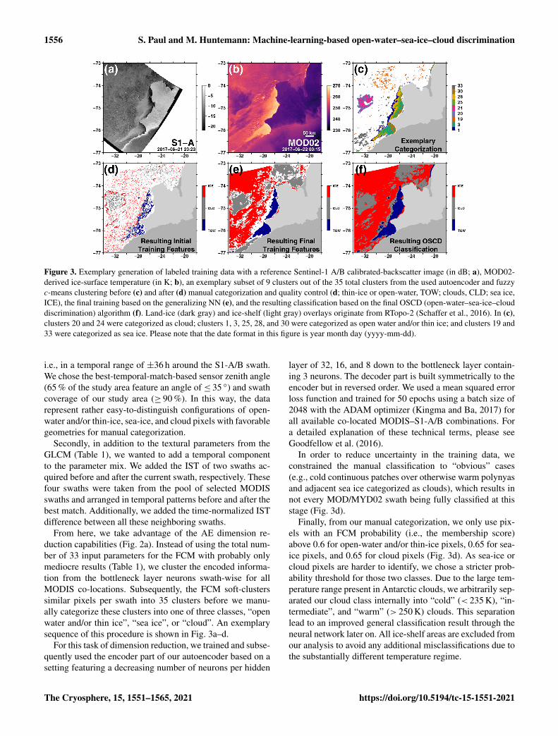
Figure 3. Exemplary generation of labeled training data with a reference Sentinel-1 A/B calibrated-backscatter image (in dB; a), MOD02-derived ice-surface temperature (in K; b), an exemplary subset of 9 clusters out of the 35 total clusters from the used autoencoder and fuzzyc-means clustering before (c) and after (d) manual categorization and quality control (d; thin-ice or open-water, TOW; clouds, CLD; sea ice,ICE), the final training based on the generalizing NN (e), and the resulting classification based on the final OSCD (open-water–sea-ice–clouddiscrimination) algorithm (f). Land-ice (dark gray) and ice-shelf (light gray) overlays originate from RTopo-2 (Schaffer et al., 2016). In (c),clusters 20 and 24 were categorized as cloud; clusters 1, 3, 25, 28, and 30 were categorized as open water and/or thin ice; and clusters 19 and33 were categorized as sea ice. Please note that the date format in this figure is year month day (yyyy-mm-dd).

i.e., in a temporal range of ±36 h around the S1-A/B swath.We chose the best-temporal-match-based sensor zenith angle(65 % of the study area feature an angle of ≤ 35 ◦) and swathcoverage of our study area (≥ 90 %). In this way, the datarepresent rather easy-to-distinguish configurations of open-water and/or thin-ice, sea-ice, and cloud pixels with favorablegeometries for manual categorization.

Secondly, in addition to the textural parameters from theGLCM (Table 1), we wanted to add a temporal componentto the parameter mix. We added the IST of two swaths ac-quired before and after the current swath, respectively. Thesefour swaths were taken from the pool of selected MODISswaths and arranged in temporal patterns before and after thebest match. Additionally, we added the time-normalized ISTdifference between all these neighboring swaths.

From here, we take advantage of the AE dimension re-duction capabilities (Fig. 2a). Instead of using the total num-ber of 33 input parameters for the FCM with probably onlymediocre results (Table 1), we cluster the encoded informa-tion from the bottleneck layer neurons swath-wise for allMODIS co-locations. Subsequently, the FCM soft-clusterssimilar pixels per swath into 35 clusters before we manu-ally categorize these clusters into one of three classes, “openwater and/or thin ice”, “sea ice”, or “cloud”. An exemplarysequence of this procedure is shown in Fig. 3a–d.

For this task of dimension reduction, we trained and subse-quently used the encoder part of our autoencoder based on asetting featuring a decreasing number of neurons per hidden

layer of 32, 16, and 8 down to the bottleneck layer contain-ing 3 neurons. The decoder part is built symmetrically to theencoder but in reversed order. We used a mean squared errorloss function and trained for 50 epochs using a batch size of2048 with the ADAM optimizer (Kingma and Ba, 2017) forall available co-located MODIS–S1-A/B combinations. Fora detailed explanation of these technical terms, please seeGoodfellow et al. (2016).

In order to reduce uncertainty in the training data, weconstrained the manual classification to “obvious” cases(e.g., cold continuous patches over otherwise warm polynyasand adjacent sea ice categorized as clouds), which results innot every MOD/MYD02 swath being fully classified at thisstage (Fig. 3d).

Finally, from our manual categorization, we only use pix-els with an FCM probability (i.e., the membership score)above 0.6 for open-water and/or thin-ice pixels, 0.65 for sea-ice pixels, and 0.65 for cloud pixels (Fig. 3d). As sea-ice orcloud pixels are harder to identify, we chose a stricter prob-ability threshold for those two classes. Due to the large tem-perature range present in Antarctic clouds, we arbitrarily sep-arated our cloud class internally into “cold” (< 235 K), “in-termediate”, and “warm” (> 250 K) clouds. This separationlead to an improved general classification result through theneural network later on. All ice-shelf areas are excluded fromour analysis to avoid any additional misclassifications due tothe substantially different temperature regime.

The Cryosphere, 15, 1551–1565, 2021 https://doi.org/10.5194/tc-15-1551-2021

S. Paul and M. Huntemann: Machine-learning-based open-water–sea-ice–cloud discrimination 1557

Table 2. List of used S1-A/B swaths for calibration or training, val-idation, and a detailed analysis (Fig. 6).

Satellite Product Acquisition in UTC

Calibration or training

S1-B IW_GRDH_1SSH 2 April 2017 03:49:42S1-A EW_GRDM_1SSH 10 April 2017 23:23:10S1-A EW_GRDM_1SSH 7 April 2017 22:58:51S1-A EW_GRDM_1SSH 18 May 2017 23:06:59S1-A EW_GRDM_1SSH 28 May 2017 00:19:56S1-A EW_GRDM_1SSH 28 May 2017 23:23:13S1-A EW_GRDM_1SSH 21 June 2017 23:23:14S1-A EW_GRDM_1SSH 3 July 2017 23:23:15S1-A EW_GRDM_1SSH 8 July 2017 00:28:10S1-A EW_GRDM_1SSH 8 July 2017 23:31:21S1-B IW_GRDH_1SSH 31 July 2017 03:49:48S1-A EW_GRDM_1SSH 8 August 2017 23:23:17S1-B IW_GRDH_1SSH 19 August 2017 23:30:41S1-A IW_GRDH_1SSH 1 September 2017 23:23:18S1-A EW_GRDM_1SSH 20 September 2017 00:11:57S1-A EW_GRDM_1SSH 25 September 2017 23:23:19

Validation

S1-A EW_GRDM_1SSH 7 April 2017 22:58:51S1-B EW_GRDM_1SSH 9 April 2017 00:27:24S1-A EW_GRDM_1SSH 11 May 2017 00:11:50S1-A EW_GRDM_1SSH 20 July 2017 00:28:11S1-A IW_GRDH_1SSH 6 August 2017 03:50:27S1-A IW_GRDH_1SSH 11 September 2017 03:50:28

Example

S1-A EW_GRDM_1SSH 16 May 2017 23:23:12S1-A EW_GRDM_1SSH 18 May 2017 23:06:59

Through this procedure, we created an initial labeled train-ing data set consisting of about 3.5× 106 data points for the33 predictors (Table 1). For the purpose of training the NN,we divided the data into a training or calibration and a vali-dation data set (Fig. 2b). As a random split would potentiallylead to highly autocorrelated neighboring pixels, we decidedfor a swath-wise split with 16 swaths used for training or cal-ibration and 6 swaths used for validation plus an additional2 swaths for an additional analysis (Table 2).

2.4 Final-training-data generation

As mentioned, the initial training data set is based solely onobvious cases that were manually categorized. This proce-dure lead to only few data points per swath (Fig. 3d). In or-der to (at least almost) fully classify all co-located MODISswaths and thereby extend our training data set, two simpleintermediate classifiers were trained to represent their respec-tive initial training data set (i.e., calibration or validation) asbest as possible (Fig. 2c).

With this, we are able to extend our training data set byidentifying and classifying additional similar data points in

the complete set of co-located MODIS swaths that were pre-viously not categorized. However, based on the class proba-bilities provided by the two NNs and through visual screen-ing, we excluded ambiguous pixels from the final trainingdata set (Fig. 3e). In this way, we get a statistically substanti-ated classification of almost the complete swaths – in contrastto the partially categorized swaths through manual classifica-tion used before (Fig. 2c).

Through this procedure, we created our final labeled train-ing data set of about 10.0× 106 and 3.1× 106 data pointscomprising the 33 different predictors or parameters for cal-ibration and validation, respectively (Table 1).

2.5 Training of the final classifier

We used this final training data set to train our final classi-fier (Fig. 2d). This NN consists of 6 hidden layers containing20 neurons each with activation functions for a leaky recti-fied linear unit (leaky ReLU) while using a fixed batch sizeof 2048, a learning rate of 1× 10−4, and a dropout rate of20 % as well as weight decay in the form of an L2 param-eter regularization (Goodfellow et al., 2016). Furthermore,we used categorical cross-entropy loss and again the ADAMoptimizer (Kingma and Ba, 2017).

Our final open-water–sea-ice–cloud discrimination(OSCD) classifier features an accuracy (the ratio of correctlyclassified pixels to the total number of samples) of 90.8 %and 84.3 % on the calibration and validation data set,respectively. For our comparisons and the results, we alwaysmerged all cloud subclasses to a single cloud class (Figs. 2eand 3f).

3 Results and discussion

In the following, we describe and discuss the results fromusing our open-water–sea-ice–cloud discrimination (OSCD)product in comparison to the reference MOD/MYD29 sea-ice product on the basis of a thin-ice thickness (TIT) esti-mates (i) on a swath-to-swath basis, (ii) on the basis of dailycomposites of all available swaths per day, and (iii) as a com-parison of overall achieved coverage over a year (Fig. 2f).

3.1 Swath-based comparison

Representative comparisons between resulting the TIT fromOSCD and MOD/MYD29 swaths reveal substantial differ-ences, especially in the high-temperature polynya and thin-ice areas (PA; Figs. 4 and 5).

The S1-A/B reference data always feature a polynya sig-nal in all our examples (Figs. 4a, e, and i and 5a, e, and i)and these are (at least partially) represented by a warm ISTanomaly in the MODIS data (Figs. 4b, f, and j and 5b, f,and j). While for some examples the difference in resultingTIT between OSCD and MOD/MYD29 is comparably smallor negligible (Figs. 4g and h and 5c and d), substantial dif-

https://doi.org/10.5194/tc-15-1551-2021 The Cryosphere, 15, 1551–1565, 2021

1558 S. Paul and M. Huntemann: Machine-learning-based open-water–sea-ice–cloud discrimination

Figure 4. Compilation of exemplary co-located S1-A/B calibrated backscatter (in dB) and MODIS swaths of ice-surface temperature (IST;in K) and derived thin-ice thickness (TIT; in m) data (Table 3). Gray and green overlays highlight the ice-shelf extent. Manually pickedS1-A/B reference polynya extent is outlined by a dashed red line in all panels. Please note that the date format in this figure is year monthday (yyyy-mm-dd).

ferences appear for other examples (Figs. 4k and l, 5g and k,and 5h and l).

For a better comparison, the polynyas were hand-pickedfor the respective S1-A/B data in Figs. 4 and 5. The corre-sponding absolute polynya areas are summarized in Table 3.In addition to the respective numbers for each polynya, thecorresponding area covered in the S1-A/B extent is given inparentheses. While there is some uncertainty due to the dif-ferent grid resolutions (25 m vs. 1 km) as well as acquisition-time difference and subsequent changes due to sea-ice drift,this allows for a good quantification of the impact of erro-neously classified cloud cover on the estimated TIT.

While there are correct and also corresponding cloud clas-sifications in both MODIS products, the applied MODIScloud mask in the MOD/MYD29 product tends towards ad-ditionally masking out strong positive temperature anomalies(Figs. 4l and 5h and l). This happens frequently in the centerof the primary polynya around 27.4◦W and 76◦ S and leadsto substantial differences in PA estimates (Table 3).

Due to the strong temperature gradient between the warmocean and the cold atmosphere, turbulent exchange of sen-sible and latent heat is large and can potentially lead to theformation of sea fog and thin, low cloud cover (Gultepe et al.,2003; Fraser et al., 2009). However, the temperature texturein the open-water and/or thin-ice areas appears to be homo-

The Cryosphere, 15, 1551–1565, 2021 https://doi.org/10.5194/tc-15-1551-2021

S. Paul and M. Huntemann: Machine-learning-based open-water–sea-ice–cloud discrimination 1559

Figure 5. Additional compilation of exemplary co-located S1-A/B and MODIS swaths in the same setup as Fig. 4. Gray and green overlayshighlight the ice-shelf extent. Manually picked S1-A/B reference polynya extent is outlined by a dashed red line in all panels. Please notethat the date format in this figure is year month day (yyyy-mm-dd).

Table 3. Summary of polynya area (PA; in km2) estimates betweenS1-A/B (PAS1), OSCD (PAOSCD), and MOD/MYD29 (PAM29)data. PA estimates in parentheses correspond to the PA retrievedfrom MODIS for the S1-A/B polygon in Figs. 4 and 5.

Example PAS1 PAOSCD PAM29

Fig. 4a–d 903 106 (0) 714 (0)Fig. 4e–h 2224 5620 (2136) 6897 (2122)Fig. 4i–l 380 989 (355) 43 (16)Fig. 5a–d 1093 892 (601) 841 (577)Fig. 5e–h 1448 1945 (858) 3366 (534)Fig. 5i–l 1425 1748 (1407) 1502 (245)

geneous and is likely not to be affected by either sea fog orclouds to the extent suggested by the MOD/MYD29 productthrough the MODIS cloud mask.

3.2 Daily-composite-based comparison

Based on the median TIT of all available MODIS swathsper day, daily polynya area (PA) was computed (Paul et al.,2015), and the difference between OSCD and MOD/MYD29was calculated (i.e., OSCD minus MOD/MYD29; Fig. 6).

Scattering of OSCD and MOD/MYD29 daily PA estimatesagainst each other reveals a general tendency towards largerPA estimates in MOD/MYD29 data (Fig. 6; top-left scat-terplot inlet). However, there is also a strong seasonality in

https://doi.org/10.5194/tc-15-1551-2021 The Cryosphere, 15, 1551–1565, 2021

1560 S. Paul and M. Huntemann: Machine-learning-based open-water–sea-ice–cloud discrimination

Figure 6. Daily polynya area difference in 103km2 using swath-wise pixel averages featuring a thin-ice thickness (TIT) ≤ 0.2 m betweenOSCD and MOD/MYD29. Difference is calculated by subtracting MOD/MYD29 from OSCD; results with OSCD≥MOD/MYD29 areshown in blue; results with OSCD<MOD/MYD29 are shown in red. Orange vertical bars highlight days with S1-A/B swath coverage usedfor calibration or training of the OSCD algorithm. Green vertical bars show additional S1-A/B swaths used for validation between products(Figs. 4 and 5). The top-left corner features a scatterplot of the daily polynya with MOD/MYD29 to OSCD. Additional information aboutthe S1-A/B swaths is provided in Table 2.

this MOD/MYD29 bias, which dominates from 1 April 2017to mid May 2017, while OSCD estimates are predominatelylarger than or equal to MOD/MYD29 between mid May and30 September 2017 (Fig. 6). For the year 2017, about 64 %,50.0 %, and 27 % of the differences of the absolute daily me-dian PA are below 1000 km2, 500 km2, and 100 km2, respec-tively.

On average, OSCD estimates the daily polynya area (PA)between 1 April and 30 September 2017 to be 1.88×103 km2

in contrast to 2.69×103 km2 using MOD/MYD29 data (notshown). This corresponds to an average daily mean PA whichis about 44 % smaller for OSCD compared to MOD/MYD29.

However, especially during freeze-up (i.e., between1 April 2017 and mid May 2017), the differences are of-tentimes very large (14.9×103 km2 on 17 May 2017) andtowards MOD/MYD29. To analyze this, we conduct a moredetailed analysis of the OSCD and MOD/MYD29 daily me-dian TIT (Figs. 7 and 8).

Unfortunately, no S1-A/B swath was acquired over theBIS area for 17 May 2017. However, S1-A/B swaths wereacquired the day before and after (Table 2).

From the S1-A/B data (Fig. 7a and b), the existence ofopen water and/or thin ice very close to the ice-shelf edgearound 27.4◦W and 76◦ S for 18 May 2017 is evident.

The lack of any clearly distinguishable positivetemperature-anomaly features in the MODIS daily me-dian IST composite (Fig. 7c) and the general texture of

rather smooth temperature patches are both signs for apersistently present cloud cover during 17 May 2017.

However, the relatively high temperatures of some of thesepotential clouds lead to an erroneous calculation of TIT andthe subsequent daily median TIT composite with an erro-neously much larger polynya area (PA) for MOD/MYD29compared to OSCD (Fig. 7d and e). Nonetheless, also OSCDfeatures TIT estimates from cloud artifacts in the northwestaround 29.5◦W and 74–74.5◦ S as well as in the area of theprimary BIS polynya.

The individual swaths used for the computation of bothcomposites underline the absence of any pronounced positivetemperature anomalies corresponding to open-water and/orthin-ice features (Fig. 8a–g).

While cold clouds are reliably identified, the inability ofthe MODIS cloud mask to also reliably identify warm cloudpatterns results in the computation of TIT in large patcheswest of BIS (Fig. 8q–u). Conversely, these false computa-tions are not present or are at least much reduced in theOSCD data (Fig. 8j–n). However, while a small area west ofthe tip of the BIS around 28◦W and 75.5◦ S corresponds wellto the polynya signal in the S1-A data (Fig. 7b), the majorityof the TIT estimates appear to be cloud artifacts (Fig. 8n).

From our analysis of the swath-based and daily-compositecomparisons, three major take home messages can be sum-marized:

The Cryosphere, 15, 1551–1565, 2021 https://doi.org/10.5194/tc-15-1551-2021

S. Paul and M. Huntemann: Machine-learning-based open-water–sea-ice–cloud discrimination 1561

Figure 7. Compilation of S1-A swaths acquired on 16 and 18 May 2017 (a, b, respectively; calibrated backscatter in dB), the daily medianice-surface temperature (IST; in K) composite for 17 May 2017 from all available MODIS swaths (c), and the resulting daily median thin-icethickness (TIT; in m) composites for the OSCD (d) and MOD/MYD29 (e) products for 17 May 2017, respectively. Red dashed line outlinesthe polynya on 18 May 2017 in S1-A. Please note that the date format in this figure is year month day (yyyy-mm-dd).

Figure 8. Compilation of MODIS swaths used for the computation of the data shown in Fig. 7: swath-based ice-surface temperature (IST inK; a–g), resulting swath-wise thin-ice thickness (TIT in m) using OSCD (h–n) and MOD/MYD29 (o–u) data, respectively. Please note thatthe date format in this figure is year month day (yyyy-mm-dd).

https://doi.org/10.5194/tc-15-1551-2021 The Cryosphere, 15, 1551–1565, 2021

1562 S. Paul and M. Huntemann: Machine-learning-based open-water–sea-ice–cloud discrimination

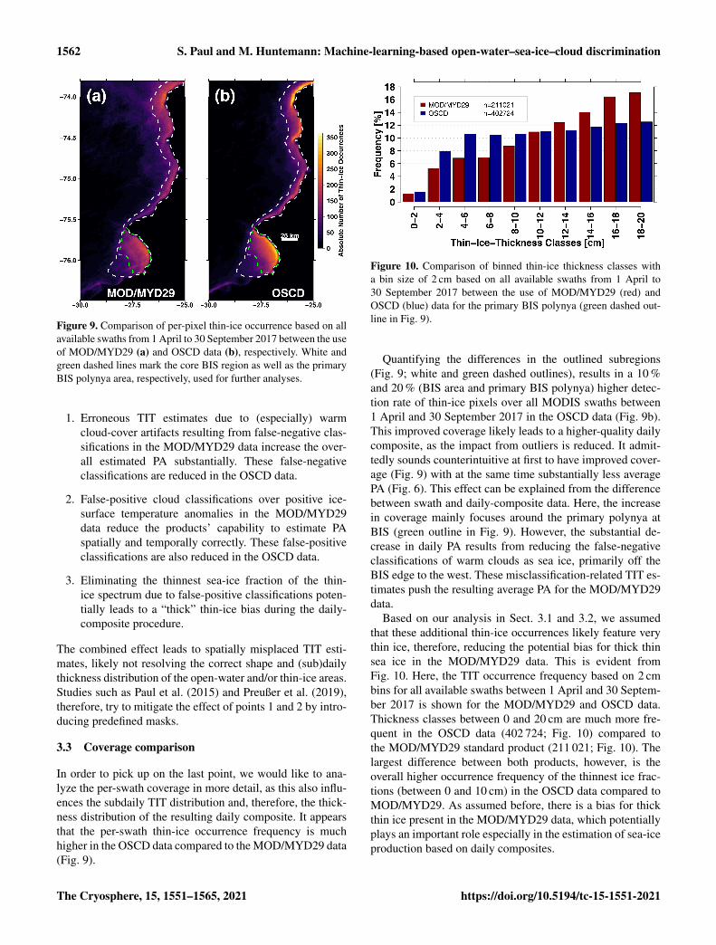
Figure 9. Comparison of per-pixel thin-ice occurrence based on allavailable swaths from 1 April to 30 September 2017 between the useof MOD/MYD29 (a) and OSCD data (b), respectively. White andgreen dashed lines mark the core BIS region as well as the primaryBIS polynya area, respectively, used for further analyses.

1. Erroneous TIT estimates due to (especially) warmcloud-cover artifacts resulting from false-negative clas-sifications in the MOD/MYD29 data increase the over-all estimated PA substantially. These false-negativeclassifications are reduced in the OSCD data.

2. False-positive cloud classifications over positive ice-surface temperature anomalies in the MOD/MYD29data reduce the products’ capability to estimate PAspatially and temporally correctly. These false-positiveclassifications are also reduced in the OSCD data.

3. Eliminating the thinnest sea-ice fraction of the thin-ice spectrum due to false-positive classifications poten-tially leads to a “thick” thin-ice bias during the daily-composite procedure.

The combined effect leads to spatially misplaced TIT esti-mates, likely not resolving the correct shape and (sub)dailythickness distribution of the open-water and/or thin-ice areas.Studies such as Paul et al. (2015) and Preußer et al. (2019),therefore, try to mitigate the effect of points 1 and 2 by intro-ducing predefined masks.

3.3 Coverage comparison

In order to pick up on the last point, we would like to ana-lyze the per-swath coverage in more detail, as this also influ-ences the subdaily TIT distribution and, therefore, the thick-ness distribution of the resulting daily composite. It appearsthat the per-swath thin-ice occurrence frequency is muchhigher in the OSCD data compared to the MOD/MYD29 data(Fig. 9).

Figure 10. Comparison of binned thin-ice thickness classes witha bin size of 2 cm based on all available swaths from 1 April to30 September 2017 between the use of MOD/MYD29 (red) andOSCD (blue) data for the primary BIS polynya (green dashed out-line in Fig. 9).

Quantifying the differences in the outlined subregions(Fig. 9; white and green dashed outlines), results in a 10 %and 20 % (BIS area and primary BIS polynya) higher detec-tion rate of thin-ice pixels over all MODIS swaths between1 April and 30 September 2017 in the OSCD data (Fig. 9b).This improved coverage likely leads to a higher-quality dailycomposite, as the impact from outliers is reduced. It admit-tedly sounds counterintuitive at first to have improved cover-age (Fig. 9) with at the same time substantially less averagePA (Fig. 6). This effect can be explained from the differencebetween swath and daily-composite data. Here, the increasein coverage mainly focuses around the primary polynya atBIS (green outline in Fig. 9). However, the substantial de-crease in daily PA results from reducing the false-negativeclassifications of warm clouds as sea ice, primarily off theBIS edge to the west. These misclassification-related TIT es-timates push the resulting average PA for the MOD/MYD29data.

Based on our analysis in Sect. 3.1 and 3.2, we assumedthat these additional thin-ice occurrences likely feature verythin ice, therefore, reducing the potential bias for thick thinsea ice in the MOD/MYD29 data. This is evident fromFig. 10. Here, the TIT occurrence frequency based on 2 cmbins for all available swaths between 1 April and 30 Septem-ber 2017 is shown for the MOD/MYD29 and OSCD data.Thickness classes between 0 and 20 cm are much more fre-quent in the OSCD data (402 724; Fig. 10) compared tothe MOD/MYD29 standard product (211 021; Fig. 10). Thelargest difference between both products, however, is theoverall higher occurrence frequency of the thinnest ice frac-tions (between 0 and 10 cm) in the OSCD data compared toMOD/MYD29. As assumed before, there is a bias for thickthin ice present in the MOD/MYD29 data, which potentiallyplays an important role especially in the estimation of sea-iceproduction based on daily composites.

The Cryosphere, 15, 1551–1565, 2021 https://doi.org/10.5194/tc-15-1551-2021

S. Paul and M. Huntemann: Machine-learning-based open-water–sea-ice–cloud discrimination 1563

Despite great care during the manual categorization, un-certainty remains due to the lack of measured ground-truthdata for the training data generation. However, the underly-ing statistical basis from the unsupervised FCM clusteringin combination with a second stage of fully classifying allco-located MODIS swaths using NNs before generating thecalibration or validation swath-split final training data for theOSCD algorithm appears to provide a realistic representationof the present sea-ice conditions in the BIS area.

4 Summary and outlook

In this study, we present a novel approach to improve the de-tection of wintertime cloud cover over Antarctic sea ice andits discrimination from sea-ice cover and open-water and/orthin-ice areas in MODIS thermal-infrared data using a deepneural network.

We established a labeled training data set using thetechniques of dimension reduction, unsupervised clustering,and supervised learning in combination with manual visualscreening and categorization. Through this effort, we gener-ated a total of 13.1×106 data points for 33 different predic-tors.

With this data set, we trained a deep neural network andused it to discriminate between open-water and/or thin-ice,sea-ice, and cloud-covered areas in the Brunt Ice Shelf re-gion for the freezing period of 2017 (1 April to 30 Septem-ber). Here, we computed the thin-ice thickness up to 0.2 m ofopen-water and/or thin-ice areas and evaluated the differencein daily polynya area and daily swath coverage to results us-ing the standard NSIDC MOD/MYD29 sea-ice product.

Based on our approach, we obtain a 44 % lower averagepolynya area but 20 % higher swath coverage rate comparedto the standard MOD/MYD29 product. On the one hand, thepolynya area in MOD/MYD29 is likely dominated throughfrequent false-negative classifications of warm clouds as thinice, leading to unrealistically large open-water and/or thin-ice areas, especially during freeze-up. On the other hand, themuch lower coverage rate likely decreases the quality and ac-curacy of TIT estimates in the daily median TIT compositeswhen using MOD/MYD29 data. Both factors are reduced inour OSCD data. This also reduces the impact of single out-liers on the daily median TIT composites and, therefore, alsoincreases the quality of derived information such as sea-iceproduction.

In the future, we plan to create an open-access comprehen-sive OSCD-based IST and TIT products covering all majorAntarctic coastal polynyas, as well as providing higher-levelparameters such as polynya area, sea-ice production, and as-sociated ocean salt flux. We expect this data set to be of greatuse to the ocean–sea-ice–ice-shelf model community as wellas for potential biological applications.

Data availability. The generated initial trainingdata set can be downloaded through Zenodo athttps://doi.org/10.5281/zenodo.4596407 (Paul, 2021). Sourcesof all used data sets are referenced in the text.

Author contributions. SP designed the study and methodology,conducted the analysis, and wrote the original draft of the paper.MH assisted in the study design and the adaptation of the machine-learning algorithms as well as with writing the paper.

Competing interests. The authors declare no conflict of interests.

Acknowledgements. The authors want to thank the LAADS DAACand the ASF DAAC for the provision of the MOD/MYD02 and S1-A/B data used here. The corresponding author appreciates the helpof his family which enabled him to finally write this paper whileworking from home due to the SARS-CoV-2 pandemic. The com-ments by two anonymous reviewers as well as the editor, ClaudeDuguay, helped to substantially improve the quality of this paper.

Financial support. The article processing charges for this open-access publication were covered by a Research Centre of theHelmholtz Association.

Review statement. This paper was edited by Claude Duguay andreviewed by two anonymous referees.

References

Ackerman, S., Frey, R., Strabala, K., Liu, Y., Gumley, L.,Baum, B., and Menzel, P.: MODIS Atmosphere L2 CloudMask Product, NASA MODIS Adaptive Processing Sys-tem, Goddard Space Flight Center, Greenbelt, USA,https://doi.org/10.5067/MODIS/MOD35_L2.006, 2015.

Adams, S., Willmes, S., Schröder, D., Heinemann, G., Bauer, M.,and Krumpen, T.: Improvement and Sensitivity Analysis of Ther-mal Thin-Ice Thickness Retrievals, IEEE T. Geosci. Remote, 51,3306–3318, 2013.

Allaire, J. and Chollet, F.: keras: R Interface to “Keras”, r pack-age version 2.3.0.0, available at: https://CRAN.R-project.org/package=keras, last access: 29 October 2020.

Atkinson, P. M. and Tatnall, A. R. L.: Introduction Neural net-works in remote sensing, Int. J. Remote Sens., 18, 699–709,https://doi.org/10.1080/014311697218700, 1997.

Aulicino, G., Sansiviero, M., Paul, S., Cesarano, C., Fusco,G., Wadhams, P., and Budillon, G.: A New Approach forMonitoring the Terra Nova Bay Polynya through MODISIce Surface Temperature Imagery and Its Validation dur-ing 2010 and 2011 Winter Seasons, Remote Sens., 10, 366,https://doi.org/10.3390/rs10030366, 2018.

https://doi.org/10.5194/tc-15-1551-2021 The Cryosphere, 15, 1551–1565, 2021

1564 S. Paul and M. Huntemann: Machine-learning-based open-water–sea-ice–cloud discrimination

Bezdek, J. C., Ehrlich, R., and Full, W.: FCM: The fuzzy c-means clustering algorithm, Comput. Geosci., 10, 191–203,https://doi.org/10.1016/0098-3004(84)90020-7, 1984.

Cao, W., Wang, X., Ming, Z., and Gao, J.: A Review on NeuralNetworks with Random Weights, Neurocomput., 275, 278–287,https://doi.org/10.1016/j.neucom.2017.08.040, 2018.

Dee, D. P., Uppala, S. M., Simmons, A. J., Berrisford, P., Poli,P., Kobayashi, S., Andrae, U., Balmaseda, M. A., Balsamo, G.,Bauer, P., Bechtold, P., Beljaars, A. C. M., van de Berg, L., Bid-lot, J., Bormann, N., Delsol, C., Dragani, R., Fuentes, M., Geer,A. J., Haimberger, L., Healy, S. B., Hersbach, H., Hólm, E. V.,Isaksen, L., Kållberg, P., Köhler, M., Matricardi, M., McNally,A. P., Monge-Sanz, B. M., Morcrette, J.-J., Park, B.-K., Peubey,C., de Rosnay, P., Tavolato, C., Thépaut, J.-N., and Vitart, F.: TheERA-Interim reanalysis: configuration and performance of thedata assimilation system, Q. J. Roy. Meteor. Soc., 137, 553–597,https://doi.org/10.1002/qj.828, 2011.

Dong, G., Liao, G., Liu, H., and Kuang, G.: A Review of the Au-toencoder and Its Variants: A Comparative Perspective from Tar-get Recognition in Synthetic-Aperture Radar Images, IEEE T.Geosci. Remote, 6, 44–68, 2018.

Drucker, R., Martin, S., and Moritz, R.: Observations ofice thickness and frazil ice in the St. Lawrence Islandpolynya from satellite imagery, upward looking sonar, andsalinity/temperature moorings, J. Geophys. Res., 108, 3149,https://doi.org/10.1029/2001JC001213, 2003.

Dunn, J. C.: A Fuzzy Relative of the ISODATA Process and Its Usein Detecting Compact Well-Separated Clusters, J. Cybernetics,3, 32–57, https://doi.org/10.1080/01969727308546046, 1973.

Fraser, A. D., Massom, R. A., and Michael, K. J.: A Method forCompositing Polar MODIS Satellite Images to Remove CloudCover for Landfast Sea-Ice Detection, IEEE T. Geosci. Remote,47, 3272–3282, https://doi.org/10.1109/TGRS.2009.2019726,2009.

Fraser, A. D., Massom, R. A., and Michael, K. J.: Generation ofhigh-resolution East Antarctic landfast sea-ice maps from cloud-free MODIS satellite composite imagery, Remote Sens. Environ.,114, 2888–2896, 2010.

Fraser, A. D., Massom, R. A., Ohshima, K. I., Willmes, S.,Kappes, P. J., Cartwright, J., and Porter-Smith, R.: High-resolution mapping of circum-Antarctic landfast sea ice dis-tribution, 2000–2018, Earth Syst. Sci. Data, 12, 2987–2999,https://doi.org/10.5194/essd-12-2987-2020, 2020.

Frey, R. A., Ackerman, S. A., Liu, Y., Strabala, K. I.,Zhang, H., Key, J. R., and Wang, X.: Cloud Detection withMODIS. Part I: Improvements in the MODIS Cloud Maskfor Collection 5, J. Atmos. Ocean. Tech., 25, 1057–1072,https://doi.org/10.1175/2008JTECHA1052.1, 2008.

Goodfellow, I., Bengio, Y., and Courville, A.: Deep Learning, MITPress, available at: http://www.deeplearningbook.org (last ac-cess: 18 January 20201), 2016.

Gultepe, I., Isaac, G. A., Williams, A., Marcotte, D., and Straw-bridge, K. B.: Turbulent heat fluxes over leads and polynyas,and their effects on arctic clouds during FIRE.ACE: Air-craft observations for April 1998, Atmos. Ocean, 41, 15–34,https://doi.org/10.3137/ao.410102, 2003.

Hall, D., Key, J., Casey, K., Riggs, G., and Cava-lieri, D.: Sea ice surface temperature product from

MODIS, IEEE T. Geosci. Remote, 42, 1076–1087,https://doi.org/10.1109/TGRS.2004.825587, 2004.

Hall, D. K. and Riggs, G. A.: MODIS/Terra Sea Ice Extent 5-minL2 Swath 1km, Version 6, National Snow and Ice Data Center,https://doi.org/10.5067/MODIS/MOD29.006, 2015a.

Hall, D. K. and Riggs, G. A.: MODIS/Aqua Sea Ice Extent 5-minL2 Swath 1km, Version 6, National Snow and Ice Data Center,https://doi.org/10.5067/MODIS/MYD29.006, 2015b.

Hall, D. K., Nghiem, S. V., Rigor, I. G., and Miller, J. A.: Uncertain-ties of Temperature Measurements on Snow-Covered Land andSea Ice from In Situ and MODIS Data during BROMEX, J. Appl.Meteor. Climatol., 54, 966–978, https://doi.org/10.1175/JAMC-D-14-0175.1, 2015.

Hall-Beyer, M.: Practical guidelines for choosing GLCM tex-tures to use in landscape classification tasks over a range ofmoderate spatial scales, Int. J. Remote Sens., 38, 1312–1338,https://doi.org/10.1080/01431161.2016.1278314, 2017.

Haralick, R. M.: Statistical and structural approaches to texture,Proc. IEEE, 67, 786–804, 1979.

Haralick, R. M., Shanmugam, K., and Dinstein, I.: Textural Featuresfor Image Classification, IEEE T. Syst. Man Cyb., 3, 610–621,1973.

Hartigan, J. A. and Wong, M. A.: Algorithm AS 136: A K-MeansClustering Algorithm, J. R. Stat. Soc. C-Appl., 28, 100–108,1979.

Holz, R. E., Ackerman, S. A., Nagle, F. W., Frey, R., Dutcher, S.,Kuehn, R. E., Vaughan, M. A., and Baum, B.: Global Moder-ate Resolution Imaging Spectroradiometer MODIS cloud detec-tion and height evaluation using CALIOP, J. Geophys. Res., 113,D00A19, https://doi.org/10.1029/2008JD009837, 2008.

Kingma, D. P. and Ba, J.: Adam: A method for stochastic optimiza-tion, arXiv [preprint], arXiv:1412.6980, 30 January 2017.

Kohonen, T.: An introduction to neural computing, Neural Net-works, 1, 3–16, https://doi.org/10.1016/0893-6080(88)90020-2,1988.

LeCun, Y., Bengio, Y., and Hinton, G.: Deep learning, Nature, 521,436–444, https://doi.org/10.1038/nature14539, 2015.

Lee, J., Weger, R. C., Sengupta, S. K., and Welch, R. M.: A neuralnetwork approach to cloud classification, IEEE T. Geosci. Re-mote, 28, 846–855, 1990.

Liu, Y. and Key, J. R.: Less winter cloud aids summer 2013 Arc-tic sea ice return from 2012 minimum, Environ. Res. Lett., 9,044002, https://doi.org/10.1088/1748-9326/9/4/044002, 2014.

Liu, Y., Key, J. R., Frey, R. A., Ackerman, S. A., and Menzel, W.:Nighttime polar cloud detection with MODIS, Remote Sens. En-viron., 92, 181–194, https://doi.org/10.1016/j.rse.2004.06.004,2004.

Ludwig, V., Spreen, G., Haas, C., Istomina, L., Kauker, F., andMurashkin, D.: The 2018 North Greenland polynya observedby a newly introduced merged optical and passive microwavesea-ice concentration dataset, The Cryosphere, 13, 2051–2073,https://doi.org/10.5194/tc-13-2051-2019, 2019.

MacQueen, J.: Some methods for classification and analysis ofmultivariate observations, Berkeley Symposium on Mathemati-cal Statistics and Probability, 5.1, 281–297, 1967.

Meyer, D., Dimitriadou, E., Hornik, K., Weingessel, A., and Leisch,F.: e1071: Misc Functions of the Department of Statistics, Proba-bility Theory Group (Formerly: E1071), TU Wien, r package ver-

The Cryosphere, 15, 1551–1565, 2021 https://doi.org/10.5194/tc-15-1551-2021

S. Paul and M. Huntemann: Machine-learning-based open-water–sea-ice–cloud discrimination 1565

sion 1.7-2, available at: https://CRAN.R-project.org/package=e1071 (last access: 14 October 2020), 2019.

MODIS Characterization Support Team (MCST): MODIS 1kmCalibrated Radiances Product, NASA MODIS Adaptive Pro-cessing System, Goddard Space Flight Center, Greenbelt, USA,https://doi.org/10.5067/MODIS/MYD021KM.06, 2017a.

MODIS Characterization Support Team (MCST): MODIS 1kmCalibrated Radiances Product, NASA MODIS Adaptive Pro-cessing System, Goddard Space Flight Center, Greenbelt, USA,https://doi.org/10.5067/MODIS/MYD021KM.06, 2017b.

Paul, S.: Manually categorized initial training data for open-water/sea-ice/cloud discrimination (Version 1.0.0) [Data set],Zenodo, https://doi.org/10.5281/zenodo.4596407, 2021.

Paul, S., Willmes, S., and Heinemann, G.: Long-term coastal-polynya dynamics in the southern Weddell Sea from MODISthermal-infrared imagery, The Cryosphere, 9, 2027–2041,https://doi.org/10.5194/tc-9-2027-2015, 2015.

Preußer, A., Ohshima, K. I., Iwamoto, K., Willmes, S., and Heine-mann, G.: Retrieval of Wintertime Sea Ice Production in ArcticPolynyas Using Thermal Infrared and Passive Microwave Re-mote Sensing Data, J. Geophys. Res.-Oceans, 124, 5503–5528,https://doi.org/10.1029/2019JC014976, 2019.

R Core Team: R: A Language and Environment for Statistical Com-puting, R Foundation for Statistical Computing, Vienna, Austria,available at: https://www.R-project.org/ (last access: 19 Novem-ber 2020), 2018.

Reiser, F., Willmes, S., and Heinemann, G.: A New Algorithm forDaily Sea Ice Lead Identification in the Arctic and AntarcticWinter from Thermal-Infrared Satellite Imagery, Remote Sens.,12, 1957, https://doi.org/10.3390/rs12121957, 2020.

Riggs, G. and Hall, D.: MODIS Sea Ice Products User Guide toCollection 6, National Snow and Ice Data Center, University ofColorado, Boulder, USA, 50 pp., 2015.

Schaffer, J., Timmermann, R., Arndt, J. E., Kristensen, S. S.,Mayer, C., Morlighem, M., and Steinhage, D.: A global, high-resolution data set of ice sheet topography, cavity geome-try, and ocean bathymetry, Earth Syst. Sci. Data, 8, 543–557,https://doi.org/10.5194/essd-8-543-2016, 2016.

Schmidhuber, J.: Deep learning in neural networks:An overview, Neural Networks, 61, 85–117,https://doi.org/10.1016/j.neunet.2014.09.003, 2015.

Toller, G., Xu, G., Kuyper, J., Isaacman, A., and Xiong, J.: MODISLevel 1B Product User’s Guide, NASA/Goddard Space FlightCenter, Greenbelt, USA, 63 pp., 2009.

Welch, R. M., Sengupta, S. K., Goroch, A. K., Rabindra, P., Ran-garaj, N., and Navar, M. S.: Polar Cloud and Surface Classifi-cation Using AVHRR Imagery: An Intercomparison of Meth-ods, J. Appl. Meteorol., 31, 405–420, http://www.jstor.org/stable/26186465 (last access: 22 October 2020), 1992.

Yu, Y. and Rothrock, D. A.: Thin ice thickness from satel-lite thermal imagery, J. Geophys. Res., 101, 25753–25766,https://doi.org/10.1029/96JC02242, 1996.

Zvoleff, A.: glcm: Calculate Textures from Grey-Level Co-Occurrence Matrices (GLCMs), r package version 1.6.4, avail-able at: https://CRAN.R-project.org/package=glcm (last access:29 October 2020), 2019.

https://doi.org/10.5194/tc-15-1551-2021 The Cryosphere, 15, 1551–1565, 2021