Improved Reconstruction Attacks on Encrypted Data Using

Range Query Leakage

Marie-Sarah Lacharitemarie-sarah.lacharite.2015@rhul.ac.uk

Brice Minaudbrice.minaud@rhul.ac.uk

Kenneth G. Patersonkenny.paterson@rhul.ac.uk

Abstract

We analyse the security of database encryption schemes supporting range queries against per-sistent adversaries. The bulk of our work applies to a generic setting, where the adversary’s viewis limited to the set of records matched by each query (known as access pattern leakage). Wealso consider a more specific setting where certain rank information is also leaked. The latter isinherent to multiple recent encryption schemes supporting range queries, including Kerschbaum’sFH-OPE scheme (CCS 2015), Lewi and Wu’s order-revealing encryption scheme (CCS 2016), andthe recently proposed Arx scheme of Poddar et al. (IACR eprint 2016/568, 2016/591). We providethree attacks.

First, we consider full reconstruction, which aims to recover the value of every record, fullynegating encryption. We show that for dense datasets, full reconstruction is possible within anexpected number of queries N logN + O(N), where N is the number of distinct plaintext values.This directly improves on a O(N2 logN) bound in the same setting by Kellaris et al. (CCS 2016).We also provide very efficient, data-optimal algorithms that succeed with the minimum possiblenumber of queries (in a strong, information theoretical sense), and prove a matching data lowerbound for the number of queries required.

Second, we present an approximate reconstruction attack recovering all plaintext values in adense dataset within a constant ratio of error (such as a 5% error), requiring the access patternleakage of only O(N) queries. We also prove a matching lower bound.

Third, we devise an attack in the common setting where the adversary has access to an auxiliarydistribution for the target dataset. This third attack proves highly effective on age data from real-world medical data sets. In our experiments, observing only 25 queries was sufficient to reconstructa majority of records to within 5 years.

In combination, our attacks show that current approaches to enabling range queries offer littlesecurity when the threat model goes beyond snapshot attacks to include a persistent server-sideadversary.

1 Introduction

Various kinds of property-preserving encryption (PPE) schemes have started to see wide deployment,in particular in the area of data storage outsourcing. There, a client encrypts a set of records ordocuments using a PPE scheme, sends it to the server, and is later able to query the server andretrieve the matching records or documents. By exploiting the special properties of the encryptionscheme, the server can index the data just as it would unencrypted data, allowing the server to supportefficient search. For example, deterministic encryption allows matching queries to be made, whileOrder-Preserving/Revealing Encryption (OPE/ORE) allow range queries to be efficiently supported.

At the same time, our understanding of the security that such schemes offer against various kindsof adversary is still developing. This has led to serious attacks being found against some of the earlyschemes [CGPR15, NKW15, GMN+16, PW16, ZKP16, DDC16, GSB+17] – a good summary of this

1

line of research is available in [FVY+17]. A second generation of schemes, which typically use customindexes rather than legacy indexes, promise to do better, in the sense of provably leaking less infor-mation about encrypted data. Perhaps inevitably, the second generation of schemes has been followedby another wave of attacks. Kellaris, Kollios, Nissim, and O’Neill introduced generic reconstructionattacks applicable to any scheme whose range queries leak access pattern or communication volume, fora uniform range query distribution [KKNO16]. Grubbs, Sekniqi, Bindschaedler, Naveed, and Risten-part presented a snapshot attack on non-deterministic, frequency-hiding OPE schemes when auxiliaryinformation about the plaintext distribution is available [GSB+17]. We continue this line of researchinto generic attacks, which apply even to second-generation encryption schemes, focussing on thoseschemes that support range queries.

1.1 Setting and Notation

Our attacks share the same general setting, which we now describe, together with the relevant notation.We let [a, b] denote the set of integers a, . . . , b (by convention [a, b] = ∅ whenever a > b).

Records, identifiers, and values. We consider a collection of R records (or documents) in adatabase, each with a unique identifier. The set of record identifiers is assumed, without loss ofgenerality, to be R = [1, R]. Each record r ∈ R contains a field with a single value val(r) from someordered set of values X of size N , on which range queries are performed. We assume, again without lossof generality, that X = [1, N ], with “<” being the usual ordering on the integers. We let Sx ⊆ [1, R]denote the set of identifiers of all records that contain value x. Each value can of course appear inmore than one record.

In our attacks, it is assumed that the set of all record identifiers is known.(This assumption isdiscussed in Section 4.2 – in any case, with uniform queries, the set of all identifiers is recovered withinO(N) queries.)

Range queries. A range query [x, y] is defined by its two end points x ≤ y in X . In our analyses,except where indicated otherwise, range queries are modelled as uniformly distributed non-emptyintervals in [1, N ], denoted by the distribution U . The uniformity assumption is briefly discussedin the next section. A range query returns, at the very least, a set of matching record identifiersM := r ∈ R : val(r) ∈ [x, y]. We also write M = S[x,y] := ∪x≤t≤y St.

Adversarial model. The adversarial setting we consider throughout is that of a persistent, passiveadversary, able to observe all communication between client and server. In the context of databaseencryption schemes, the word persistent is used by contrast with a snapshot adversary, who wouldonly have access to a single snapshot of the server’s memory at a particular time. The goal of theadversary is to reconstruct some information about the (plaintext) content of the encrypted databasehosted on the server, i.e. infer information about the client’s data.

Such a model captures two distinct threats. The first is that of an adversary having compromisedthe server for a sufficient length of time, or a man-in-the-middle attacker intercepting communicationsbetween client and server. The second, and more immediate one, is the scenario where the server itselfis an honest-but-curious adversary: indeed, the server is obviously able to observe all communicationbetween the client and itself. From this perspective, the security model we consider directly expressesthe privacy of the user’s data with respect to the server. In particular we emphasise that all our attackscould be mounted by the server itself (and ultimately show that the schemes under consideration offerlittle privacy for the user’s data with the respect to the host server).

Since some database encryption scheme is used, the adversary is in general not able to observequeried ranges or other plaintext values. Instead, the view of the adversary is limited to some scheme-dependent leakage induced by each range query. In this article, two models are considered for thisleakage, which we now present.

2

1 2 3 4 5

1 2 3

2 3 5 1 4

Record IDs R:

Values X :

Sorted record IDs:

val

rank

Figure 1: Example of mappings val and rank.

Access pattern leakage. As explained above, it is assumed that an adversary is able to observesome information leaked by range queries. If the leakage is limited to the set of matching recordidentifiers M as defined above, following [KKNO16], we call this leakage access pattern leakage. Asdiscussed in [KKNO16], access pattern leakage can stem from the actual access pattern of the server,so long as memory accesses reveal which records are read. In this context the ID of a record is itsmemory address. This is a rather generic setting: to the best of our knowledge, all known efficientschemes supporting range queries leak the access pattern.

Rank information leakage. In addition, some of our attacks exploit rank information leakage.Although an attacker does not see the exact values of the end points x and y, it may learn someinformation regarding their rank. The rank of a value z ∈ X is the number of records having a valueless than or equal to z:

rank(z) := |S[1,z]|.

The rank of a value z can be interpreted as the highest position or index a record in Sz can have in alist of records sorted by value. In such a list, the position of any record r having value z = val(r) mustfall between rank(z − 1) + 1 and rank(z), where by convention rank(0) := 0. The exact format of rankleakage can vary, and we discuss how it is leaked for some particular schemes in Section 1.3.

A simple illustration is provided in Figure 1. Here we take R = 5, N = 3, with val(1) = val(4) = 3,val(2) = val(3) = 1, and val(5) = 2. In that case, as pictured, we have rank(1) = 2, rank(2) = 3, andrank(3) = 5.

For a query on range [x, y] (unknown to the attacker) matching recordsM, the rank leakage is thevalues a := rank(x− 1) and b := rank(y). The values a+ 1 and b can be interpreted as the lowest andhighest positions (inclusive) of records in M, within a list of records sorted by value. Note that thenumber of records returned by the query on range [x, y] satisfies:

|M| =∑x≤t≤y |St|

= rank(y)− rank(x− 1)

= b− a.

Whenever we consider intervals of values in [1, N ], we shall use the letters [x, y]; whenever we considerintervals of ranks (generally the image of some values in [1, N ] via rank), we shall use the letters [a, b].

Overall, if leakage is limited to the access pattern, then a query on range [x, y] leaks M = S[x,y].If, in addition, rank information leakage is available, then the leakage of a query on range [x, y] is(a, b,M) where a = rank(x− 1), b = rank(y), and M = S[x,y]. When a set of queries is considered asan input to an adversary observing their leakage, we will often assimilate the set of queries with theirleakage. In this context we write the input of the adversary as a set of triplets Q = (ak, bk,Mk) ifrank information is available, or simply Q = Mk if only the access pattern is available.

3

Req’d leakage Assumptions Number of queries

Rank Density Sufficient Necessary

Full reconstruction attack[KKNO16] N N O(N4 logN) Ω(N4)[KKNO16] N Y O(N2 logN) -Sec. 2.3 (Algo. 1) Y Y N(logN + 2) N log(N)/2−O(N)Sec. 2.4 (Algo. 2) N Y N(logN + 3) N log(N)/2−O(N)

Approximate reconstruction attack (within εN)Sec. 3.2 (Algo. 3) N Y 5

4N log(1/ε) +O(N) N log(1/ε)/2−O(N)

Table 1: Comparison of full and approximate reconstruction attacks exploiting access pattern leakageon encryption schemes allowing range queries, for a set of N distinct plaintext values, with uniformly

distributed queries.

Density of the database. We say that the database is dense iff every value x ∈ [1, N ] occurs in atleast one record. We will generally assume that the database is dense, except in Section 4. Wheneverthis assumption is necessary, formal statements will always mention it explicitly.

Miscellaneous mathematical notation. The notation log will always refer to the natural loga-rithm, rather than logarithm in base 2. We write Hn for the n-th harmonic number Hn =

∑nk=1

1k .

Whenever f is a mapping A→ B, if S ⊆ A, f(A) denotes the image set f(a) : a ∈ A.

1.2 Our Contributions

In this paper, we analyse the security of encryption schemes supporting range queries against persistentadversaries. The bulk of our work applies to the generic setting where the view of the adversary islimited to the set of matched records per query (access pattern leakage). We additionally considerthe special case where the leakage contains rank information. It is natural to consider such leakagein schemes supporting range queries, and our attacks directly apply to, among others, Lewi and Wu’sORE scheme, Arx-Range, and Kerschbaum’s frequency-hiding OPE scheme; more applications arediscussed in Section 1.3.

In total we present three different, but related, attacks: full reconstruction, approximate recon-struction, and reconstruction using auxiliary information. An overview of the characteristics of ourfirst two attacks, juxtaposed with previous results, is given in Table 1. Note that without rank leakage,full reconstruction is only up to reflection. In Table 1, the exact upper bounds on the expected numberof queries for the attacks in Sections 2.3 and 2.4 require N ≥ 27 and N ≥ 26 respectively.

Full reconstruction attack. We show that access pattern leakage is sufficient to allow full recon-struction, i.e. recovering the value of all records with complete accuracy (up to reflection), withinan expected number of only N logN +O(N) queries, where N is the number of distinct values. Thisdirectly improves on a O(N2 logN) bound by Kellaris et al. in the same setting [KKNO16]. Fur-thermore this can be achieved both data-optimally, in the sense that as soon as the available leakageis sufficient for full reconstruction in an information theoretic sense, our algorithms do succeed; andefficiently. We note that the hidden constants in our data requirements are quite small; a bound forthe expected number of queries is N(log(N) + 3) for N ≥ 26.

In the setting where rank leakage is also available, we give an algorithm for full reconstruction,with a slightly better bound of N(log(N) + 2) queries for N ≥ 27. Moreover the algorithm is stilldata-optimal in the previous sense, and especially efficient (incurring very little overhead over readingthe query leakage). Finally, we also prove a lower bound of N log(N)/2 − O(N) on the expected

4

number queries required for full reconstruction from access pattern leakage, for any algorithm, with orwithout rank information.

As explained in the previous section, our attacks are in the fully passive honest-but-curious setting,wherein a server stores the encrypted database, and processes a set of queries from a client, but hasno additional powers otherwise. In particular, the server cannot make chosen queries of its own (if itcould, then there are trivial reconstruction attacks requiring only N queries); and no knowledge aboutthe distribution of values is assumed. We require only two mild extra assumptions for the attacks tosucceed:

1. every x ∈ X appears in at least one record (so the sets Sx are non-empty), also referred to as“density” in [NKW15, KKNO16];

2. the range queries [x, y] are generated uniformly at random.

One benefit of assuming uniformly random range queries is that it makes our work directly compa-rable to Kellaris et al.’s [KKNO16]. However, as already discussed, our full reconstruction algorithmsare data-optimal. As a consequence these algorithms consume the minimum possible amount of datafor any query distribution. Thus the uniformity assumption plays no role in the design of the algorithm.Instead the assumption is used to compute data upper bounds. As we also show, very similar boundswould be obtained for the distribution where left end points are uniformly random; more generally, weconjecture that similar bounds would be achieved for a wide range of “non-pathological” distributions.(This is by contrast to e.g. Kellaris et al.’s attack in the non-dense case, which relies on a statisticalinference approach that directly exploits the expected distribution of range queries.)

As intuition for the attack when rank leakage is available, consider the simpler situation wherethe x values appearing in the queried ranges [x, y] are uniformly random.1 Then with Ω(N logN)queries, with high probability, every possible x value occurs at least once. This is a consequence ofthe standard analysis of the coupon collector’s problem. The different x values are easily identifiedsince they correspond to different values of rank(x− 1) and the latter leaks to the adversary. It is thenpossible to recover the sets Sx with some simple set manipulations. What we show is that this simpleexample can be refined into a data-optimal algorithm that encompasses the case of uniformly randomqueries; and, perhaps surprisingly, that it can be extended to the generic setting where only accesspattern leakage is available.

As a concrete example, if the values x represent age in years and we have N = 125, then ourattack reduces by a factor of about 100 the number of queries that need to be observed for completereconstruction, as compared to [KKNO16]. Specifically, their attack requires an expected number of

queries N(N+1)2 HN(N+1)/2 ≈ 75, 196 queries. On the other hand, the expected number of queries for

full reconstruction with our attack is at most (N + 1)(log(N) + 1) + 8√N + 6 ≈ 830 queries, or, if rank

leakage is available, N(log(N) + 1) + 4.4√N + 4 ≈ 782 queries (here we use the tighter bounds from

Propositions 1 and 2). Thus the gap is significant even for relatively low values of N .

Approximate reconstruction attack. In some situations, exactly recovering the value x associatedwith each record is not necessary, and it may be sufficient to approximately learn these values. Forexample, the values may pertain to age or salary, and for the attacker, learning only an approximationmay be good enough.

In this situation, we show that, under the same assumptions as our first attack, O(N) queriessuffice, even in the general setting where only the access pattern is leaked. More precisely, within anexpected number of 5

4N log(1/ε) +O(N) queries, the attacker can reconstruct the values x associatedwith every record with a maximum error of εN , for any arbitrary precision ε. In particular, the datarequirement only grows logarithmically with the desired precision ε. Once again the hidden constantsare quite reasonable: an exact upper bound is (1 + ε/4)N log(1/ε) + (2 + 4

√ε)N + 4/ε for N ≥ 40. We

1If [x, y] is generated uniformly at random, by choosing one of the possible intervals with equal probability, then xis not uniformly random, but rather weighted towards low values, with, for example x = N appearing with probabilityonly 2/(N(N + 1)).

5

also prove a lower bound N log(1/ε)/2−O(N) on the expected number of queries before any algorithmcan achieve approximate reconstruction with precision εN .

The intuition behind this improvement over the full reconstruction attack is that, as discussed,our first attack ultimately reduces to solving a variant of the coupon collector’s problem on the set[1, N ], with the x-values in the range queries [x, y] playing the role of coupons. However, collectingthe last few coupons is relatively expensive, and most of the coupons can be procured with O(N)queries. Moreover, collecting most of the coupons is sufficient to approximately reconstruct the valuesassociated to all records.

Going back to the example whereN = 125, the approximate reconstruction attack starts to overtakethe full reconstruction attack (without rank information) for ε ≈ 0.05, i.e. when reconstructing recordsup to a precision of 5%. Per our definition of precision, this means that for all records, the attackerhas successfully determined an interval of size 0.05 ·N containing the value of the record; in particular,if the attacker were to guess the value of each record as the middle of the corresponding interval, thentheir guess would never be wrong by more than 2.5% of N . For a precision of 10% (which allowsestimating the value of all records up to 5%), the required number of queries is at most 744, comparedto 830 for full reconstruction. (Of course this gap grows with N : for N = 10000, the ratio of theexpected number of queries for the former attack compared to the latter is about half.)

Inference attack using an auxiliary distribution. Recent research has shown that an attackerequipped with an auxiliary (or reference) distribution for the plaintext can wreak havoc against deter-ministic encryption schemes in a snapshot attack model by using basic frequency analysis [NKW15].The assumption that an auxiliary distribution is available is a mild one in practice, for it is often thecase that the type of data in a given column in an encrypted database is known or can be inferredfrom the diversity of its values [NKW15], and a rough and ready auxiliary distribution can be obtainedfrom public statistics.

In our third attack, we show how an auxiliary distribution can be combined with rank and accesspattern leakage to perform even better reconstruction attacks. The main insight is that the rankleakage from each query can be converted into information about the position of individual records inthe ordered list of all records (such a list is intrinsic to schemes like Arx). By analysing the appearancesof each record in response to multiple queries, the possible range of positions in which that record liescan be gradually constrained. The final range for that record is then mapped back to a small set ofpossible values using the inverse CDF of the auxiliary distribution. We show how to exploit theseideas to obtain more accurate attacks with fewer queries. Because this third attack is not amenableto a rigorous analysis, we resort to an empirical evaluation. In particular, we study the relationshipbetween number of random range queries available and the accuracy of reconstruction of “age in years”data, extracted from a real-world medical dataset. In our experiments, observing only 50 queries wassufficient to reconstruct 95% of one hospital’s records to within 10 years, 55% of its records to within 5years, and 35% of its records to within 3 years. With more than 100 queries, our experimental resultswere limited only by the accuracy of the auxiliary distribution.

1.3 Applications

To the best of our knowledge, all practical encryption schemes supporting range queries leak accesspattern information. This makes our generic attacks requiring only access pattern leakage widelyapplicable. However, it should be noted that schemes such as [BLR+15, CLWW16] that rely on order-preserving or order-revealing encryption (OPE/ORE) are already vulnerable to powerful statisticalinference attacks by snapshot adversaries, such as [NKW15].2

As a consequence, our attacks are more relevant to second-generation schemes that attempt toreduce or eliminate leakage against snapshot adversaries. These schemes can be divided into twogroups: schemes that leak access pattern but not rank, and those that also leak rank information. The

2In particular, any ORE (a fortiori OPE) scheme in the strict sense, i.e. where there exists a public algorithmenabling order comparison on ciphertexts, is trivially broken whenever the database is dense, as ordering all ciphertextsallows them to be directly matched with plaintext values.

6

first group includes Blind Seer by Pappas et al. [PKV+14], as well as a scheme by Faber et al. [FJK+15];they also include approaches based on Range Predicate Encryption, such as [Lu12]. These schemesare vulnerable to our full and approximate reconstruction attacks.

The second group includes a variety of recent schemes [LW16, YGW+17, PBP16, Ker15, RACY16,HK16, AEJ+15]. In the remainder of this section, we look at some of these schemes in more detailand explain how they leak rank information. Since all of the schemes listed below leak rank infor-mation, they are vulnerable to all of our attacks. In addition to the schemes that are listed below,the recent POPE scheme by Roche et al. [RACY16], and a scheme with similar leakage by Hahn andKerschbaum [HK16], should also be mentioned: although these two schemes mainly target scenarioswhere the database is not dense, our third attack remains applicable.

Lewi-Wu scheme. At CCS 2016, Lewi and Wu introduced a new practical construction for order-revealing encryption [LW16]. This construction also serves as the basis for supporting range queriesin EncKV [YGW+17]. The Lewi-Wu scheme is not strictly an order-revealing scheme; in particular,it is fully secure against a basic snapshot adversary. One of the key ideas of the Lewi-Wu scheme isto allow encryption of plaintext values into two types of ciphertexts, named left and right ciphertexts.The database itself only contains right ciphertexts, which are semantically secure. Meanwhile rangequeries are handled by sending to the server left ciphertexts for both ends of the range. Left ciphertextscan be compared (in the sense of order comparison) with right ciphertexts using a public algorithm,which allows the server to identify values in-between the two end points of the range. However inthis process, the server also learns which values are below the lower end point, and in particular thenumber of these values; and likewise for values above the higher end point. Thus rank information isleaked to the server.

Arx. Arx is a second-generation scheme recently proposed by Poddar et al. [PBP16]. In the previousreference, the authors mention ongoing collaboration with health data cloud provider Chino and Eu-ropean medical project UNCAP to deploy their scheme. Amongst other features, Arx builds a specialArx-Range index [BPP16] to support efficient range queries on encrypted data. Such an index is builtfor each field that will need to be ordered or queried by range.

The security of Arx is proven in terms of leakage; security theorems establish that the scheme doesnot leak more than is captured by the leakage functions as observed by a persistent, honest-but-curiousadversary playing the role of the server [PBP16, Appendix A]. In general, the leakage of a query is thetype of query, the time it was issued, and which records or fields are accessed, but not their content,nor any constants in the query. For a range query on interval [x, y], the Arx-Range paper [BPP16,Theorem 8.1] states that the rank of the values x− 1 and y is leaked in addition to the access patternS[x,y]. In particular, the values of x and y are not (directly) leaked by the range queries, and, beingencrypted, the contents of each matching record are not leaked. The Arx-Range index does actuallyleak the rank and identifier set, so the leakage model is exact, and our attacks apply.

FH-OPE. Another example of a second-generation scheme is Kerschbaum’s frequency-hiding, order-preserving encryption (FH-OPE) scheme [Ker15]. This scheme ensures that the same plaintext is neverencrypted twice to the same ciphertext, thus thwarting basic frequency analysis attacks for a snapshotattacker (cf. [NKW15]), but also preserves order, so that range queries are easy to perform on encrypteddata. At a high level, the scheme operates as follows. The client’s state records the possible range ofencrypted values for each plaintext value. Using this state, the client can rewrite a query for values inthe range [x, y] to one for values in the range [min(x),max(y)], where min(z) and max(z) are bounds onthe minimum and maximum size of ciphertexts corresponding to the value z. This scheme can be castin the same terminology as we have used above, with FH-OPE ciphertexts corresponding to records(and their identifiers) and values x corresponding to plaintexts. It is then immediately apparent thatthe scheme leaks rank information. This is because queries leak the values of min(x) and max(y)to a persistent, honest-but-curious adversary playing the role of the server, and this adversary can

7

always compute exact information about the ranks of x and y by comparing min(x) and max(y) tothe complete set of (ordered) ciphertexts.

Cipherbase. Our attacks also apply to Cipherbase [AEJ+15], an encrypted database system thatuses a combination of custom equality and range indices and trusted hardware. The range indexis a B-tree, whose nodes each contain a number of encrypted value-record ID pairs, sorted by value.Traversing the tree is done by performing a series of order comparisons, outsourced to a trusted module,which decrypts and compares two values. By observing the access pattern as the tree is traversed tofind the endpoints of a range query, an attacker learns the set of matching record IDs (by looking atthose between the two endpoints) and the ranks of two values (by counting how many values are tothe “left” of the endpoints in the B-tree). Thus, even though the scheme uses IND-CPA encryptionand a secure hardware module, the sorted nodes in the range index and the access pattern provideenough leakage for our attacks.

For all of the aforementioned schemes except FH-OPE, the only attacks we are aware of besideours is that of Kellaris et al. [KKNO16], which mainly focuses on the non-dense setting, and requiresa significantly larger number of queries. In the non-dense case, the approach of Kellaris et al. is touse statistical inference based on the uniformity of queries; in the dense case, they collect all O(N2)possible queries, resulting in a simple sorting step.

In the particular case of Kerschbaum’s FH-OPE scheme [Ker15], an attack was already mountedby Grubbs et al. [GSB+17]. Their attack is in the snapshot setting and thus did not use query leakage.Attacks of a similar nature against OPE and ORE schemes can also be found in [DDC16]. Althoughour attacks require query leakage, they are more generic, as the scheme is only required to leak accesspatterns (and in some cases rank information). Another difference is that the attack by Grubbs et al.requires knowledge of an auxiliary distribution, whereas our first two attacks (full and approximatereconstruction) do not.

2 The Full Reconstruction Attack

The purpose of a full reconstruction attack is to determine the sets Sx for all x ∈ X . In other words,a full reconstruction attacks recovers the value associated with every record.

2.1 Setup of the Attack and Layout of the Section

We assume that an honest user of the system makes a sequence of Q randomly generated range queries[x, y], each query returning a set of records M = S[x,y]. Since we are in the persistent, honest-but-curious setting, the set of matching records M is learned by the adversary – this is the access patternleakage.

In Section 2.2, we start with a simple introductory example. In Section 2.3, we focus on the casewhere range queries leak rank information, as defined in Section 1.1. In Section 2.4, we show how theattack can be extended to work with only access pattern leakage. Throughout this section, we assumethat the database is dense, i.e. every value appears in at least one record (cf. Section 1.1).

In all cases, we prove that N logN +O(N) queries are enough for full reconstruction (and provideconcrete bounds). In Appendix C, we prove a matching lower bound. An important note is that,throughout this section, we give algorithms that favour simplicity over efficiency. In Appendix A, weshow how these algorithms can be made (much) more efficient.

2.2 A Simple Example

As a warm-up, we begin with an example that provides some intuition for why N logN+O(N) queriesare enough for full reconstruction in the presence of rank information leakage. For simplicity, in thescope of this example, we assume that the left end points x of range queries [x, y] are uniformly random.

8

In the rest of the article, this will not be the case, because we will instead assume that range queriesare uniformly random (which implies that left end points are biased toward lower values).

Recall that each query on an interval [x, y] returns the set of record identifiers whose value lies in[x, y], that is:

S[x,y] := r ∈ R : val(r) ∈ [x, y].

We let Mk = S[xk,yk] denote the set of identifiers returned for the k-th query on range [xk, yk]. Alsorecall that ak = rank(xk− 1), bk = rank(yk) denote the rank information leaked by the k-th query. Foreach query on range [xk, yk], the adversary is able to observe the leakage (ak, bk,Mk), but not directlyxk or yk.

Success condition. The following algorithm will succeed iff every value x ∈ [1, N ] appears as theleft end point of some query. Because we assumed uniformly random left end points, the expectednumber of queries until this condition is satisfied is exactly the standard coupon collector’s problem.As such, using standard arguments, it is equal to:

N ·HN ≤ N

(1 +

∫ N

x=1

1

x

)= N(1 + logN)

where HN is the N -th harmonic number. We now assume that the condition is satisfied: every leftend point occurs in at least one query.

The algorithm. By reordering and relabelling, we may assume that the ak’s are in increasing order(so ak+1 ≥ ai for each i). Because every x value occurs in at least one query, there are exactly Ndistinct ak values, each corresponding to one of the N different entries in X ; in particular we must havea1 = 0, corresponding to value 1. The adversary selects any N -subset of indices ki, where 1 ≤ i ≤ N ,such that the aki are all distinct. It then computes:

Ei =Mki \

⋃`≥ki+1

M`

, 1 ≤ i ≤ N

where we define the union ∪`≥ki+1M` for i = N to be the empty set.

It is not hard to see that the set Ej is precisely the set of record identifiers for records containingvalue j ∈ X , that is, Ej = Sj . The idea is thatMkj certainly contains all such records, but possibly alsoadditional records (because the range of query kj contains j but possibly other values too). Performinga set subtraction with the sets of record identifiers M` for ` ≥ kj+1 removes the additional records.

This concludes our description of the attack: within an expected number of queries N · HN ≤N log(N) + N , all left end points are collected; and we have just seen that as a result, the value ofall records can be recovered. Despite its simplicity, this example captures a large part of the intuitionbehind our attacks in this section and the next. In particular, the data complexity bounds in thefollowing sections are ultimately based on reductions to (increasingly intricate) variants of the couponcollector’s problem.

2.3 The Full Reconstruction Attack with Rank Information

Before moving on to full reconstruction attacks without rank information, we first present a more robustalgorithm for full reconstruction in the presence of rank information leakage, which improves on thealgorithm from the previous section in various ways. The general approach of this new algorithm, andin particular the notion of partition of records, will form the basis of later algorithms and their analysis.This new algorithm is also data-optimal, in the sense that if the algorithm fails, then full reconstructionis impossible for any algorithm given the input queries. As a consequence, this algorithm requires theminimum possible number of queries for any distribution of queries.

9

In particular, it must perform at least as well as the algorithm from the previous section in terms ofthe required number of queries, so it succeeds within an expected number of queries ≤ N(log(N) + 1)in the case of uniform left end points. Moreover we will show that it also succeeds with an expectednumber of queries ≤ N(log(N) + 2) for uniform queries (contrary to the algorithm from the previoussection, which requires Ω(N2) queries in that setting3).

The algorithm. The idea of the algorithm is as follows. As before, fix a set of Q queries on ranges[xk, yk], k ≤ Q. The corresponding leakage observed by the adversary is (ak, bk,Mk) : k ≤ Q, whereak = rank(xk − 1), bk = rank(yk), and Mk = S[xk,yk] is the set of records with values in [xk, yk].

Define the following equivalence relation on records (recall that records are assimilated with theirIDs). Two records are equivalent iff for all Q queries, either both records are matched by the query, orneither. At least intuitively, it is clear that two records can only be meaningfully distinguished giventhe set of queries iff they are in distinct equivalence classes. Moreover, the equivalence class of a recordr can be easily computed as:

P (r) =

( ⋂k:r∈Mk

Mk

)∖( ⋃k:r 6∈Mk

Mk

).

Since Mk = r ∈ R : val(r) ∈ [xk, yk], P (r) contains exactly those records whose value lies in:

V (r) =

( ⋂k:r∈Mk

[xk, yk]

)∖( ⋃k:r 6∈Mk

[xk, yk]

).

Note that neither P (r) nor V (r) can be empty, as they must contain at least, respectively, r and val(r).Note also that V (r) is unknown to the adversary at this point in the attack.

To sum up, the set of P (r)’s (resp. V (r)’s) forms a partition of the set of records (resp. values), andeach P (r) contains exactly those records whose value lies in V (r). Due to this bijection, the partitionof records P = P (r) : r ∈ R cannot contain more than N elements. On the other hand, since recordsin the same class cannot be meaningfully distinguished, full reconstruction requires |P| = N .

The crucial point is that, conversely, the condition |P| = N is enough to enable full reconstruction.Indeed, if |P| = N , then by the bijection with the V (r)’s, each V (r) must contain a single value, andP (r) constitutes the set of records having that value. Thus each element of P corresponds to a singlevalue: P = Sx : x ∈ X. Hence, in order to find the value of every record, it only remains to sortthe elements of P by value. But this can be done using rank as a kind of proxy for value. Indeed, thevalue of P (r) has rank

m(r) = max

( ⋂k:r∈Mk

[ak, bk]

)∖( ⋃k:r 6∈Mk

[ak, bk]

) .

Then it suffices to sort all values m(r) to correctly sort the corresponding classes P (r) by value.Our algorithm does exactly this. Pseudo-code is provided in Algorithm 1. In this algorithm, weimmediately compute the map m, and check that m(r) : r ∈ R = N . First computing P and/or Vis not necessary in this setting, but is only used above as an aid to understanding the algorithm.

Analysis of the algorithm. We make several claims about Algorithm 1. The first is that it is data-optimal, i.e. if the algorithm fails, then no algorithm can achieve full reconstruction with probability1 given the same queries as input. The rationale we have provided for the algorithm already givesstrong evidence that this is the case (which is to say, |P| = N is a necessary condition); however amore formal treatment is provided in Appendix D. Second, we observe that Algorithm 1 still achieves

3For the uniform distribution U on ranges, left end points within [N − c,N ] for any fixed constant c, only occur withprobability Θ(1/N2) – cf. Lemma 1 in Appendix B.1 for an exact distribution.

10

Algorithm 1 Full reconstruction attack with rank information.

Full-Reconstruction(Q):Input: set of queries Q = (ak, bk,Mk).Output: ⊥, or map Val : R → X s.t. ∀r Val(r) = val(r).

1: m← empty map, Val← empty map2: for all r ∈ R do . Partitioning step

3: m(r)← max((⋂

k:r∈Mk[ak, bk])\(⋃k:r 6∈Mk[ak, bk]

))4: end for5: M ← m(r) : r ∈ R6: if |M | < N then7: return ⊥8: end if9: Sort M in increasing order . Sorting step

10: for all r ∈ R do11: Val(r)← index of m(r) in sorted M . Counting from 112: end for13: return Val

full reconstruction with an expected number of queries upper-bounded by N(log(N)+1) in the settingwhere left end points are uniformly random. This is a direct consequence of data optimality and theobservations in Section 2.2.4

More importantly, we claim that, unlike the algorithm from Section 2.2, Algorithm 1 achieves asimilar data complexity in the case where range queries are uniformly random. More precisely, we showthat for N ≥ 27, the expected number of queries is upper-bounded by N(log(N) + 2). For simplicity,in the following statement, we assume that N is a multiple of 4; it is clear that the success probabilityof the algorithm, and the expected number of queries before it succeeds, respectively increase anddecrease with N , so we can always round N to the next multiple of 4 if necessary.

Proposition 1. Assume N is a multiple of 4. Assume that the database is dense, and range queriesare drawn uniformly at random. Then the probability of success of Algorithm 1 after Q queries islower-bounded by:

1− 2e−Q/(2N+2) −Ne−Q/N .

Moreover, the expected number of queries before the algorithm succeeds is upper-bounded by:

N log(N) +O(N).

Concretely, for N ≥ 27, it is upper-bounded by N(log(N) + 1) + 4.4√N + 4 ≤ N(log(N) + 2).

A proof of Proposition 1 is given in Appendix B.2. As a concrete example, setting N = 100yields an expected number of queries upper-bounded by 609 to achieve full reconstruction, regardlessof the number of records, as long as the database is dense (i.e. every value occurs at least once). Weemphasise that full reconstruction means recovering the value of every single record.

Matching lower bound. In Appendix C, we investigate whether Ω(N logN) queries are in factnecessary for full reconstruction. Corollary 1 answers in the positive, showing that the expectednumber of queries for any algorithm to achieve full reconstruction is 1

2N log(N)−O(N).

4Indeed data optimality implies that if for some distribution D on the set of queries, there exists an algorithm thatachieves full reconstruction with an expected number of queries E, then for the same distribution the expected numberof queries necessary for Algorithm 1 to succeed is at most E.

11

Complexity. For clarity, Algorithm 1 is stated in a way that closely follows the rationale exposedearlier in this section. However it is quite inefficient: line 3 in particular results in a large numberof redundant computations, each involving multiple intersections and unions of potentially large sets.Keep in mind that in a real-world database, while the number of values N may be small, and wealready know that Q ≈ N logN queries are enough for full reconstruction, the number of records Rcan be quite large. In Appendix A, we show a very efficient approach to computing the partition ofrecords, without explicitly computing any set intersections or unions. This results in a time complexityO(Q(N +R)), with little overhead over simply reading all queries.

2.4 The Full Reconstruction Attack with only Access Pattern Leakage

In the previous section, we studied full reconstruction in the presence of rank information leakage. Wenow extend the attack to the case where only the access pattern is leaked. That is, for each query, onlythe set of IDs for records matching the query is leaked to the adversary, and nothing else. Kellaris etal. have already shown that O(N2 logN) queries are enough to achieve full reconstruction for densedatabases [KKNO16]. However, we show that N log(N) + O(N) queries are still enough. As before,our assumptions are that range queries are uniformly distributed, and that the database is dense. Theattack requires no a priori knowledge about the distribution of values among records.

A small caveat is that in the absence of rank information, full reconstruction can be achieved onlyup to reflection. By reflection, we mean the permutation of values that swaps value i with valueN + 1− i. The point is that if we compose the mapping val from records to values with this reflection,and also apply it to the end points [x, y] of range queries (which preserves the uniform distribution), allelse remaining equal, then access pattern leakage is unchanged. As a result, if we make no assumptionabout the distribution of values among records, an adversary whose view is restricted to access patternleakage can only hope to recover the mapping val of records to values up to reflection. The sameis of course true for the attacks in [KKNO16]. As a consequence, whenever we talk about (full)reconstruction with only access pattern leakage, we mean full reconstruction up to reflection (which,on the other hand, is possible, as we shall see).

The algorithm. Recall that the adversary only has access to queries on ranges [xk, yk], and only seesthe access pattern leakageMk = S[xk,yk]. In the remainder we identify a query with the correspondingset of matching records. We note that the algorithm can fail at a few points; however Proposition 7in Appendix D shows that the algorithm is data-optimal, i.e. whenever it fails, although this may notbe immediately apparent, full reconstruction was in fact impossible. The attack can be divided into apartitioning step and a sorting step.

The partitioning step is essentially identical to the attack from the previous section. Indeed, wecan compute the partition of records P as introduced in Section 2.3:

P =

( ⋂k:r∈Mk

Mk

)∖( ⋃k:r 6∈Mk

Mk

): r ∈ R

.

Once again, observe that full reconstruction requires |P| = N . Conversely if |P| = N every element ofP is the set Sx of records with value x for some x ∈ X = [1, N ]. We will call the elements of P points(though the reader should keep in mind that each point is in general a set of records). Each point pcorresponds to a distinct value in X (viz. the singleton val(p)).

To achieve full reconstruction, it remains to assign the correct value to each point. This is equivalentto sorting P according to the value of each point. This is the sorting step. In the presence of rankinformation, the sorting step was essentially trivial. With only the access pattern, we proceed asfollows. First, we set out to find an end point, i.e. a point with value 1 or N . Due to the reflectionsymmetry mentioned earlier, these two cases cannot be distinguished.

In order to find an end point, we form a maximal union S of queries that does not cover the fullset of records, while ensuring that this union covers an interval of values. To ensure that the union of

12

two queries covers an interval of values, it is enough to require that the two queries overlap (indeedthe union of two overlapping intervals is an interval). Hence we build S as follows: we start with aquery not covering the full set of records, and extend it for as long as possible with overlapping queriesuntil we can no longer do so without covering the full set of records R. The crux of the matter is thatif R \ S is reduced to a single point, then it must be an end point. Indeed in that case S must coveran interval of N − 1 values within [1, N ], so the remaining value can only be 1 or N . If R \ S is not asingle point, the algorithm fails.

Once an end point is identified, we assume that it corresponds to value 1 (which must be true upto reflection). We have thus determined the initial segment of points I(1) containing a single point.We then propagate this information by building each initial segment of points I(i) = S[1,i] in turn, byinduction. Given an initial segment I(i), this amounts to finding the next point, which must be Si+1.To do this, we build the intersection T of all queries overlapping I(i) and containing at least one pointoutside I(i). We then subtract from T all queries overlapping T from the right (i.e. overlapping Tand not contained in I(i) ∪ T ) so long as T remains non-empty. If the resulting T contains a singlepoint, it must be Si+1; we let I(i+ 1) = I(i) ∪ T and continue. Otherwise the algorithm fails.

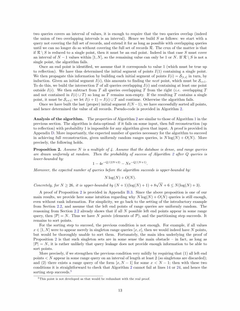
Once we have built the last (proper) initial segment I(N−1), we have successfully sorted all points,and hence determined the value of all records. Pseudo-code is provided in Algorithm 2.

Analysis of the algorithm. The properties of Algorithm 2 are similar to those of Algorithm 1 in theprevious section. The algorithm is data-optimal: if it fails on some input, then full reconstruction (upto reflection) with probability 1 is impossible for any algorithm given that input. A proof is provided inAppendix D. More importantly, the expected number of queries necessary for the algorithm to succeedin achieving full reconstruction, given uniformly random ranges queries, is N log(N) + O(N). Moreprecisely, the following holds.

Proposition 2. Assume N is a multiple of 4. Assume that the database is dense, and range queriesare drawn uniformly at random. Then the probability of success of Algorithm 2 after Q queries islower-bounded by:

1− 4e−Q/(2N+2) −Ne−Q/(N+1).

Moreover, the expected number of queries before the algorithm succeeds is upper-bounded by:

N log(N) +O(N).

Concretely, for N ≥ 26, it is upper-bounded by (N + 1)(log(N) + 1) + 8√N + 6 ≤ N(log(N) + 3).

A proof of Proposition 2 is provided in Appendix B.3. Since the above proposition is one of ourmain results, we provide here some intuition regarding why N log(N) + O(N) queries is still enough,even without rank information. For simplicity, we go back to the setting of the introductory examplefrom Section 2.2, and assume that the left end points of range queries are uniformly random. Thereasoning from Section 2.2 already shows that if all N possible left end points appear in some rangequery, then |P| = N . Thus we have N points (elements of P), and the partitioning step succeeds. Itremains to sort points.

For the sorting step to succeed, the previous condition is not enough. For example, if all valuesx ∈ [1, N ] were to appear merely in singleton range queries [x, x], then we would indeed have N points,but would be thoroughly unable to sort them. Fortunately, the main idea underlying the proof ofProposition 2 is that such singleton sets are in some sense the main obstacle – in fact, as long as|P| = N , it is rather unlikely that query leakage does not provide enough information to be able tosort points.

More precisely, if we strengthen the previous condition very mildly by requiring that (1) all left endpoints < N appear in some range query on an interval of length at least 2 (so singletons are discarded);and (2) there exists a range query of the form [x,N − 1] for some x < N − 1; then with these twoconditions it is straightforward to check that Algorithm 2 cannot fail at lines 14 or 24, and hence thesorting step succeeds.5

5This point is not developed as that would be redundant with the real proof.

13

Algorithm 2 Full reconstruction attack with only access pattern.

Full-Reconstruction-AP(Q):Input: set of queries Q = Mk.Output: ⊥, or map Val : R → X s.t. ∀r Val(r) = val(r) or ∀r Val(r) = N + 1− val(r).

1: P ← empty map, I ← empty map, Val← empty map2: for all r ∈ R do . Partitioning step

3: P (r)←(⋂k:r∈MkMk

)\(⋃k:r 6∈MkMk

)4: end for5: P ← P (r) : r ∈ R6: if |P| < N then7: return ⊥8: end if9: Pick S ∈ Q s.t. |S| < R . Sorting step

10: while ∃q ∈ Q s.t. q ∩ S 6= ∅, q \ S 6= ∅, q ∪ S 6= R do . Searching for end point11: S ← S ∪ q12: end while13: if R \ S 6∈ P then . Ensuring |val(R \ S)| = 114: return ⊥15: end if16: I(1)← R \ S . Found end point17: for all i ∈ [1, N − 1] do . Searching for the next point18: Q′ ← q ∈ Q : q ∩ I(i) 6= ∅, q \ I(i) 6= ∅19: T ←

(⋂q∈Q′ q

)\ I(i)

20: while ∃q ∈ Q s.t. q ∩ T 6= ∅, q \ (T ∪ I(i)) 6= ∅, T \ q 6= ∅ do21: T ← T \ q22: end while23: if T 6∈ P then . Ensuring |val(T )| = 124: return ⊥25: end if26: I(i+ 1)← I(i) ∪ T . Found next point27: end for28: for all r ∈ R do . Success29: Val(r)← min i : r ∈ I(i)30: end for31: return Val

In the proof of Proposition 2 (Appendix B.3), the actual requirements are slightly more intricate.This is because range queries are assumed to be uniformly distributed, which implies that neither leftnor right end points are uniformly distributed (instead, their distribution is close, respectively, to themin and max of two uniform values). However the underlying idea is the same.

Complexity. As already mentioned, our algorithms are described in an effort to maximise legibilityand ease of analysis, rather than efficiency. However in Appendix A, we show that Algorithm 2 canbe executed efficiently, in time complexity O(Q(N2 +R)).

3 The Approximate Reconstruction Attack

In the previous section, we showed that N log(N) + O(N) randomly distributed range queries aresufficient to recover the exact value x contained in every record, a full reconstruction attack. However,if we are content with recovering the value associated with every record up to a margin of error, say,

14

εN for some fixed arbitrary ε > 0, (e.g. if we wish to recover the value of all records within 1%), thenwe show in this section that the required number of queries is only O(N). We limit our attention tothe general setting where only access pattern leakage is available (a data-optimal variant when rankinformation is available is given in Appendix A).

More formally, an approximate reconstruction attack seeks to determine the value val(r) of everyrecord r, up to some precision k = εN . That is, for every record r, an approximate reconstructionattack with precision k outputs an interval [x, x+k] such that val(r) ∈ [x, x+k]. A full reconstructionattack may be regarded as the special case where k = 0. In the remainder however, we shall assumek > 0: the case k = 0 requires special treatment, and was already covered in the previous section.Without loss of generality, we may assume that k = εN is an integer. Note that our algorithm willeither succeed, i.e. it correctly recovers all values up to precision ε as defined above; or it outputs ⊥.(In other words, the algorithm can fail with ⊥, but it cannot output an incorrect answer.)

The main result of this section is an approximate reconstruction attack for which the expectednumber of queries necessary for success is upper-bounded by 5

4N log(1/ε) +O(N). In particular, it isO(N) for any fixed ε, and only grows logarithmically with the precision ε. We stress that our attackexploits only access pattern leakage and does not require rank leakage.

3.1 Intuition for the Approximate Reconstruction Attack

Before proving this result, we provide some intuition as to why the complexity drops from O(N logN)to O(N) when a margin of error is allowed in a reconstruction attack.

The reason why recovering the value of every record required O(N logN) queries is because theproblem essentially reduced to a coupon collector’s problem on N items, as seen in Section 2.2. Eachcoupon was an integer in the interval [1, N ]. After k < N distinct coupons have been drawn, drawinga new coupon requires N/(N − k) tries on average, since each new draw has a probability (N − k)/Nof yielding a new coupon, distinct from the k coupons already collected. It follows that the expectednumber of draws to gather all N coupons is:

N−1∑k=0

N

N − k= N

N∑k=1

1

k= N ·HN

where HN is the N -th harmonic number.A simple observation however is that the last few coupons are much more expensive to collect than

the early ones, in terms of the expected number of draws required. Indeed, the last coupon requires Ndraws on average, the previous one N/2 draws, etc. In particular, if we only wish to recover (1− ε)Ncoupons for some ε > 0, then the expected number of draws is:

N−εN−1∑k=0

N

N − k= N

N∑k=εN+1

1

k< N

∫ N

εN

1

x= N log

(1

ε

)where εN is assumed to be an integer. Thus, the expected number of tries is O(N), with the growthbeing proportional to log(1/ε).

3.2 Algorithm for the Approximate Reconstruction Attack

With the above intuition in mind, we now present an approximate reconstruction algorithm. As usual,we assume that the database is dense, and that range queries are uniformly distributed. No assumptionis made about the a priori distribution of values among records. The input of the algorithm, i.e. theview of the adversary, is limited to access pattern leakage. Recall from Section 2.4 that with accesspattern leakage, we can only recover record values up to reflection, i.e. we cannot distinguish betweenthe real assignment of values r 7→ val(r), and its reflection r 7→ N+1−val(r). A fortiori, the algorithmalso succeeds if rank information is available (and in that case, the limitation that values are recoveredup to reflection disappears).

15

Compared to the full reconstruction algorithms from Section 2, particular care must be takenaround a few issues. The main one is that, because the partition of records P at the core of theprevious algorithms no longer satisfies |P| = N , there is no guarantee that its elements correspond tointervals of values (as opposed to arbitrary subsets). As a result we eschew this approach, and insteadensure at every step that the subsets of records we build correspond to intervals of values (i.e. forevery subset S of records built in the course of the algorithm, val(S) is an interval). Our main tooltoward this purpose are two elementary observations: an intersection of intervals is an interval, and aunion of overlapping intervals is an interval.

The algorithm. Suppose we are given access to a set of queries Q = Mk : k ≤ Q on ranges[xk, yk], with Mk = S[xk,yk]. Our strategy for approximate reconstruction proceeds in two steps.

(1) First, we want to split the set of records into two “halves”, as follows. Let r be an arbitrary record(all possible choices of this record will be tried until the algorithm succeeds). Let M denote theintersection of all queries containing r. We wish to find two sets of records halfL and halfRsuch that halfL ∪ halfR contains all records, halfL ∩halfR = M , and finally both val(halfL) andval(halfR) are intervals. The point of this setup is that it partitions the set of records into threesubsets: halfL \M , M , and halfR \M ; such that the corresponding sets of values val(halfL \M),val(M), and val(halfR \M) is a partition of [1, N ] into three successive intervals. We will thensort records independently in halfL and halfR.

The exact technique used to build halfL and halfR is given in lines 3-6 of Algorithm 3. The ideais to build each subset as a union of two overlapping queries. This ensures that the correspondingvalue set is an interval, while incurring only a cost O(N) in the expected number of queries forthe algorithm to succeed.

(2) The next step is to sort records within halfL \M . To do so, define a left coupon as a set of recordsof the form q\halfR such that q is a query (i.e. q =Mk for some k) containing M . We claim thatthe set CL of left coupons is linearly ordered for ⊂. To see this, shift the perspective from recordsto their values: let [xM , yM ] = val(M); then every left coupon is equal to S[x,xM−1] for somex < xM . Indeed, any query q containing M is such that val(q) = S[x,y] for some x ≤ xM ≤ y,and val(halfR) = [xM , N ]. The linear order ⊂ on left coupons clearly implies the (reverse) orderfor the value of new records appearing in each successive coupon. Thus we have identified andsorted nL = |CL| distinct sets of records, all below xM .

We repeat the process for halfR to partition halfR into nR = |CR| ordered subsets, all above yM .Finally we have thus sorted nL+nR+1 distinct subsets of records, whose union covers all records.6

Since the values appearing in each subset of the global partition must be distinct, the valuesappearing in the k-th subset must be at least k; likewise they can be at most k+N−(nL+nR+1)(since the `-th set counting from the right can contain values at most N + 1 − `). Hence ifnL + nR + 1 = (1− ε)N , we have succeeded in approximate reconstruction with precision εN . Ifthat condition is not satisfied, pick the next value of r at step (1) and try again.

Pseudo-code is provided in Algorithm 3.

Analysis of the algorithm. Contrary to Algorithms 1 and 2, Algorithm 3 is not data-optimal.However a data-optimal variant in the case where rank information is available is given in Appendix A.

The main feature of Algorithm 3 is expressed by the following proposition. As before, we assumefor simplicity that N is a multiple of 4; note that the expected number of queries for the algorithm tosucceed is monotone increasing in N , so this has little impact.

6Recall that we assume [1, N ] to be a query; or equivalently, that the set of all records is known. As a result S[1,xM−1],S[yM+1,N ] must appear, respectively, as left and right coupons.

16

Algorithm 3 Approximate reconstruction attack with only access pattern.

Approximate-Reconstruction-AP(Q):Input: set of queries Q = Mk, real 0 < ε < 1.Output: ⊥, or maps minVal,maxVal : R → X s.t. ∀r, val(r) ∈ [minVal(r),maxVal(r)] or∀r, val(r) ∈ [N + 1−maxVal(r), N + 1−minVal(r)]; and ∀r,maxVal(r)−minVal(r) ≤ εN .

1: for all r ∈ R do2: M ←

⋂k:r∈MkMk . Partitioning step

3: Find qL, qR s.t. qL ∩ qR = M , maximizing |qL ∪ qR|4: Find q′L s.t. q′L ∩ qL 6= ∅, q′L ∩ qR ⊆M , maximizing |q′L ∪ qL|5: Find q′R s.t. q′R ∩ qR 6= ∅, q′R ∩ qL ⊆M , maximizing |q′R ∪ qR|6: if q′L ∪ qL ∪ qR ∪ q′R = R then7: halfL ← q′L ∪ qL8: halfR ← qR ∪ q′R9: CL ← q \ halfR : q ∈ Q,M ⊆ q \ ∅ . Left sorting step

10: nL ← |CL|11: (CL[1], . . . , CL[nL|)← sort CL for order ⊂ . It is a linear order12: CR ← q \ halfL : q ∈ Q,M ⊆ q \ ∅ . Right sorting step13: nR ← |CR|14: (CR[1], . . . , CR[nR])← sort CR for order ⊂ . It is a linear order15: if N − (nL + nR + 1) ≤ εN then16: for all r ∈ R do . Success17: if r ∈ halfL then18: minVal(r)← nL + 1−mini : r ∈ CL[i]19: else if r ∈M then20: minVal(r)← nL + 121: else if r ∈ halfR then22: minVal(r)← nL + 1 + mini : r ∈ CR[i]23: end if24: maxVal(r)← minVal(r) +N − (nL + nR + 1)25: end for26: return minVal, maxVal27: end if28: end if29: end for30: return ⊥

Proposition 3. Assume N is a multiple of 4, εN/2 is an integer, and ε < 3/4. Assume that thedatabase is dense, and range queries are drawn uniformly at random. Then the probability of successof Algorithm 3 after Q queries is lower-bounded by:

1− 4e−Q/(2N+2) − 2e−Q log(1+ε/2)+εN/2·(log(1/ε)+1.5).

Moreover, the expected number of queries before the algorithm succeeds is upper-bounded by:

5

4N log(1/ε) +O(N).

Concretely, for N ≥ 40, it is upper-bounded by (1 + ε/4)N log(1/ε) + (2 + 4√ε)N + 4/ε.

A proof of Proposition 3 is given in Appendix B.4. As a corollary of the expected number of queriesgiven above, if we want to recover the value of all records within a constant additive error, i.e. ε =Θ(1/N), then O(N logN) queries suffice: as one might expect, this matches the full reconstructionattack. Another observation is that for fixed ε, O(N) queries suffice; and perhaps surprisingly, theexpected number of queries only grows logarithmically with the desired precision.

17

The formula for the probability of success may appear difficult to parse. It may help to observethat the last term is dominant for small ε. Furthermore, for the sake of providing some intuition, ifwe approximate log(1 + ε/2) by ε/2, and disregard the final “+1.5”, then the last term would dictatea probability of failure upper-bounded by 2/e < 3/4 for Q = N log(1/ε) + 2/ε queries, and this upperbound would be divided by e ≈ 2.7 for every additional 2/ε queries. Once again if ε = Θ(1/N) thismatches the approximate behaviour of the full reconstruction attack.

Matching lower bound. In Appendix C, we investigate whether Ω(N log(1/ε)) queries are in factnecessary for approximate reconstruction. Proposition 5 in Appendix C answers in the positive, show-ing that the expected number of queries before any algorithm can achieve approximate reconstructionwith precision εN is at least 1

2N log(1/ε)−O(N) (where the constant in O(N) is independent of ε).

Complexity. As was the case with Algorithms 1 and 2, Algorithm 3 was defined with legibility inmind, rather than efficiency. A more efficient variant is discussed in Appendix A, and achieves a timecomplexity O(Q(N2 +R)) with only access pattern leakage, and O(Q(N +R)) with rank information.

4 Exploiting Auxiliary Information

Up to this point, we have focussed on trying to recover the values associated with records, withoutmaking any assumptions about the distribution of those values. However, in a real-world scenario, thisdistribution may be quite predictable.7 For instance, the values might represent the age of patients ina hospital or salaries in a personnel database. In this context, the auxiliary information provided by aknown distribution of values can help predict the values of some records, even if relatively few rangequeries are available.

In this section, we propose a heuristic algorithm for performing reconstruction attacks againstschemes that have rank leakage (such as Lewi and Wu’s ORE scheme, Arx, and FH-OPE) in thesetting where this auxiliary distribution is available. Thus our attack will now make use of rankleakage, access pattern leakage, and the auxiliary distribution. Our attack is not amenable to rigorousanalysis, unlike our previous two attacks, so we will rely on an empirical evaluation of its performance.

While we introduce a new assumption about the availability of pertinent auxiliary information, wealso remove an assumption that applied to previous attacks: we no longer assume the data is dense. So,while query end points are still sampled uniformly at random from X , not all of these values necessarilycorrespond to a record or records. As in the previous attacks, we assume that the adversary knowsthe set of record identifiers R and we treat this set as [1, R] without loss of generality.

4.1 The Algorithm

Setup. As usual, we consider the scenario where a client is issuing uniformly distributed range querieson ranges [xk, yk] ⊆ X , for k ≤ Q. For each query on range [xk, yk], the adversary observes the leakage(ak, bk,Mk), where the access pattern leakage M = S[xk,yk] = r ∈ R : val(r) ∈ [xk, yk] contains theset of matching records IDs; and the rank information leakage ak = rank(xk−1), bk = rank(yk) is suchthat [ak + 1, bk] can be interpreted as the positions of the records in Mk within a fixed list L of allrecords sorted by value (cf. Section 1.1).

The algorithm. Let us define the position of a record in L as follows: the position pos(r) of arecord r is its position in the sorted list L (counting from 1). From this perspective, the rank of avalue x is the position of the last record with value x. The algorithm proceeds in two steps. In Step 1,based on available queries, for each record r, we compute an interval [a, b] such that pos(r) ∈ [a, b]:that is, the position pos(r) of r in the list L of sorted records must lie within [a, b]. Equivalently,rank(val(r)− 1) + 1 ≥ a and rank(val(r)) ≤ b.

7We note in passing that this predictability is a necessity for the more standard line of attacks on database encryptionschemes based on statistical inference; in this regard our previous attacks are atypical.

18

Essentially we are performing an approximate reconstruction attack, except instead of outputting aninterval of X containing val(r), we output an interval of [1, R] containing pos(r). The point of workingwith the position of records is that in Step 2 of the algorithm, we will use the auxiliary informationabout the a priori distribution of values X to map each position to the most likely associated value.

To see why this makes sense, consider the following minimal example. Assume that the set of valuesX is limited to 3 values; and the a priori distribution on values tells us that they occur among recordswith respective probability 2/3, 1/6, 1/6. Then if we know that the position of r lies within [1, b] forb ≈ R · 2/3 (which could potentially be learnt from a single query via its rank leakage), we can predictthat it is likely to be 1. Compared to the algorithms we have encountered in the previous sections,such an approach can output a guess for the value of a record even when only few range queries areavailable.

We now explain each step of the algorithm in detail.Step 1. As noted earlier, determining a possible range for the position of each record is essentially

the same as an approximate reconstruction attack in the presence of rank information. Indeed it canbe realised in a straightforward manner using the ideas introduced in Section 2.3. Namely, recall thatthe partition of records P = P (r) : r ∈ R is defined by:

P (r) =

( ⋂k:r∈Mk

Mk

)∖( ⋃k:r 6∈Mk

Mk

).

In the same way, define the partition of positions S(r) : r ∈ R by:

S(r) =

( ⋂k:r∈Mk

[ak + 1, bk]

)∖( ⋃k:r 6∈Mk

[ak + 1, bk]

).

Recall that [ak + 1, bk] can be interpreted as the positions of records in Mk: that is, [ak + 1, bk] =pos(Mk). By looking at the definitions of P (r) and S(r), it is apparent that as a direct resultS(r) = pos(P (r)). Thus, S(r) contains precisely the set of positions that record r can occupy in alist of records sorted by value. As result, computing the minimal and maximal possible position of arecord r is straightforward: they are precisely min(S(r)) and max(S(r)). This concludes Step 1 of thealgorithm. Pseudo-code is provided in Algorithm 4.

Algorithm 4 Computing minimal intervals containing the position of each record.

Input: query leakage Q = (ak, bk,Mk) for k ∈ [1, Q].Output: maps minPos,maxPos : R → [1, R] s.t. ∀r, pos(r) ∈ [minPos(r),maxPos(r)].

1: S ← empty map2: for all r ∈ R do3: S(r)←

(⋂k:r∈Mk[ak + 1, bk]

)\(⋃k:r 6∈Mk[ak + 1, bk]

)4: minPos(r)← min(S(r))5: maxPos(r)← max(S(r))6: end for7: return minPos,maxPos

Step 2. At this point, for each record r, we have computed a possible range [a + 1, b] for theposition of r: we know that record r lies within range [a + 1, b] in the ordered list of records (i.e.pos(r) ∈ [a + 1, b]). From this information, we would like to output an estimate for the value val(r)of r. For this purpose, we proceed in two steps: first, from the knowledge of a, b, we compute an(approximation of) the distribution of val(r); second, using this distribution, we output an estimatefor val(r). Let us call these two steps (2a) and (2b); we now explain each step in turn. In the remainderwe fix a record r and the corresponding interval of positions [a+ 1, b] output by Algorithm 4.

(2a) Note that by construction, a and b are always the rank of some value. Moreover we can attemptto determine these values using knowledge of the auxiliary distribution D: in essence, we evaluate

19

rank(x) for all values x based on D, and match a (resp. b) with the closest result. The ideais that this yields a simple model for the distribution of val(r): namely if a = rank(x − 1) andb = rank(y), then val(r) ∈ [x, y], so we can model the distribution of val(r) as D restricted to[x, y]. We now describe this algorithm in more detail.

The auxiliary distribution D on values tells us that each value z ∈ [1, N ] occurs within records

with some probability pz, with∑Nz=1 pz = 1. Let qz =

∑zi=1 pi denote the cumulative distribu-

tion. Note that we no longer assume that every value occurs in at least one record.8

For z ∈ [1, N ], rank(z) can be seen as a random variable whose distribution is determined by D.The distribution of rank(z) is easily verified to follow a binomial distribution:

Pr [rank(z) = a] =

(R

a

)qaz (1− qz)R−a (1)

and its expected value is E(rank(z)) = Rqz.

Given a ∈ [1, R] and knowing that a = rank(z) for some z, finding the most likely value of zamounts to choosing z so as to maximise Pr [rank(z) = a].9 Fixing a, observe that the functionq 7→ qa(1−q)R−a is concave and reaches its maximum for q = a/R. Using (1), it follows that theoptimal choice of z is either z or z+ 1, for z such that a/R lies within [qz, qz+1]. In other words,as one might expect, if a lies between E(rank(z)) and E(rank(z+ 1)), then the most likely choicefor rank−1(a) is either z or z+ 1. The optimal choice between z and z+ 1 can be determined bycomputing (1) above and picking the higher of the two values.

In this way, we can compute the most likely values x, y ∈ X such that a = rank(x − 1) andb = rank(y). Assuming that rank−1(a) and rank−1(b) are in fact x− 1 and y, then val(r) ∈ [x, y],and we can model the distribution of val(r) as D restricted to [x, y], i.e. each value t ∈ [x, y]

occurs with probability (∑yi=x pi)

−1pt. This concludes the first step.

(2b) We now have (an approximation of) the distribution of val(r). We wish to output an estimateof val(r). A simple choice is to output its expected value. For the distribution proposed inthe previous step, this means outputting as a guess for val(r) the expectation of a value drawnaccording to D conditioned on being within [x, y], namely:(

y∑i=x

pi

)−1( y∑i=x

i · pi

). (2)

This concludes the attack.

Variants for Step 2. As a preliminary remark, we stress that although the previous approach forStep 2 is grounded on relevant analysis, and performs well in practice, it remains heuristic. Indeed,define the set of boundaries as the image of rank; the name boundary comes from the fact that bound-aries separate distinct values in the sorted list of records L. From this perspective, each query leakstwo boundaries ak and bk. At a high level, the problem at hand is to compute the distribution of x, yconditioned on knowing rank(x− 1) = a, rank(y) = b, and on the knowledge of all other known bound-aries ak and bk.10 In the above approach, we disregard boundaries other than a and b, and tackle eachof them in isolation, which is a reasonable approximation, but not a perfect one. Although computing

8As a side note, asking that values of records follow a distribution D cannot ensure density for N > 1, e.g. all recordscould have the same value with non-zero probability. More fundamentally, following a distribution D as above modelsthe values of records as being drawn independently for each record, while asking that every value appears at least oncerequires some interdependency.

9This can be formalised using an application of maximum likelihood estimation.10Empirical solutions for a similar but distinct problem, akin to finding the most likely simultaneous assignment of all

boundaries, are proposed in [NKW15, GSB+17].

20

the likelihood of a given assignment of boundaries to values is simple enough (it follows a multino-mial distribution), solving the previous problem that takes into account all boundaries simultaneously,seems to require, at least naively, searching a space of size exponential in N .

A number of trade-offs between accuracy and processing power are possible however. In the re-mainder, we mention a few such optimisations for step (2a). Regarding step (2b) of the algorithm, wealso briefly discuss other choices for the final estimate of val(r), depending on what metric we wish tooptimise.

Starting with step (2a), one possibility is to compute the assignment of both ends of the interval[a, b] simultaneously. That is, instead of computing za and zb to maximise Pr [rank(za) = a] andPr [rank(zb) = b] independently, maximise the joint probability Pr [rank(za) = a ∧ rank(zb) = b], whichfollows a trinomial distribution:

Pr [rank(za) = a ∧ rank(zb) = b] =R!

a!(b− a)!(R− b)!qaza(qzb − qza)b−a(1− qzb)R−b. (3)

Another possibility is to observe that in the original approach as well as the one just above, we firstcompute the most likely values x, y such that rank(x− 1) = a and rank(y) = b, then approximate thedistribution of val(r) by D restricted to [x, y]. In other words we are forcing rank−1(a) and rank−1(b)to take their most likely values and deducing the distribution of val(r) from there. We could insteadcompute the entire distribution of x and y conditioned on rank(x−1) = a and rank(y) = b, using either(1) or (3); then use this entire distribution to infer that of val(r). More explicitly, the distribution ofval(r) becomes:

Pr [val(r) = t] =∑

(x,y)∈X 2

Pr [val(r) = t|rank(x− 1) = a ∧ rank(y) = b]

·Pr [rank(x− 1) = a ∧ rank(y) = b] (4)

where the first term is equal to Pr [val(r) = t|val(r) ∈ [x, y]] = (∑yi=x pi)

−1pt and the second term can

be computed using (3). A merit of this approach is that it fully captures the information leaked bypos(r) ∈ [a, b]. It does, however, remain heuristic as already discussed – in the sense that we are stillignoring the existence of other known boundaries.

In step (2b), we use the approximation Dv of the distribution of val(r) output by step (2a) toproduce an estimate e for val(r). We chose to output the expected value of x for x← Dv. If we definethe error as the difference x − e between x ← Dv and the estimate e, then the choice of picking theexpectation ensures that the mean error is zero, and also minimises the variance of the error.11 Othermetrics we may wish to minimise include the mean of the absolute error |x− e|; in that case we shouldpick the median of the distribution as our estimate; or we may prefer to minimise the median of theabsolute error, which amounts to finding an interval [s, t] ⊆ X of minimal length and probability atleast 1/2, and outputting (s+ t)/2 (finding such an interval can be done in time O(N)).

Finally, we note that the algorithm could output more than simply an estimate of the value. Itcould, for example, simply output Dv; or, after estimating the most likely values for x and y, outputthe entire range [x, y]. Alternatively, the algorithm could compute a confidence interval around theestimated value from (2). This is straightforward using the approximate distribution output by step(2a). Such a confidence interval would be particularly meaningful if the distribution is computed asin (4), since it would then properly capture situations where a boundary falls in the middle of manysuccessive values with low probability, which can introduce a significant amount of uncertainty.

We note that in our experiments, the simple approach presented in Step 2 already proved to beeffective in practice. See further discussion in Section 4.2 below.

Complexity. Step 2 requires a negligible amount of computation (for the variant we chose). Re-garding Step 1, as in previous sections, Algorithm 4 can be sped up considerably using the techniques

11To see this, if Dv assigns probability pi to x = i, then the variance of the error is∑

i pi(i − e)2; it has degree twoin e and derivative 2(e− E [Dv ]), so its minimum is reached for e = E [Dv ].

21

from Appendix A. In fact Algorithm 5 from Appendix A can be naturally adapted to compute thesame output as Algorithm 4: it suffices to replace lines 25 and 27 in Algorithm 5 by minH ← `i + 1and maxH ← `i+1 respectively. In this way Step 1 can be computed very efficiently in O(Q(N + R))operations, in little more time than it takes to read all queries.

4.2 Experimental Results

Since this attack is less amenable to rigorous analysis, we carry out an empirical evaluation by simulat-ing queries on age data. The data we use are from the 2009 Nationwide Inpatient Sample (NIS), fromthe Healthcare Cost and Utilization Project (HCUP), run by the Agency for Healthcare Research andQuality in the United States [Age09]. (We expect results for any other year would be similar.) TheNIS is the largest publicly available inpatient database in the United States that includes dischargedata for all types of payers. It includes data at the hospital level – e.g. number of discharges, numberof beds – and at the patient discharge level – e.g. demographics, diagnosis, procedure, payer.

We extract the age data (in years) from the patient discharge records of the largest 200 hospitalsin the 2009 sample. Each of these largest hospitals has between 13,000 and 122,000 records, approx-imately, for a total of about 4.9 million records. We simulate range queries on individual hospitals’data and attack the query leakage; the auxiliary distribution we use is obtained by averaging over all200 largest hospitals’ records. Query end points are sampled independently and uniformly at randomfrom [0, 124], the range of valid age values according to the NIS Description of Data Elements. Theauxiliary attack does not require the data to be dense and, indeed, some of the ages in this rangedo not appear in the records of any of the largest 200 hospitals. Further, each hospital’s data is notnecessarily dense with respect to the auxiliary distribution.

We measure the attack’s success by computing the proportion of a hospital’s records that wasrecovered within ε, i.e. the fraction of records for which the guessed value is at most εN years awayfrom the true value, where N is the number of possible values, 125. It is important to note thatε is used only to characterise results and is not a parameter of the attack, unlike the approximatereconstruction attack in Section 3. Here, there is no guarantee that the guessed values are within ε ofthe true values.

We display results from our experiments in plots with relative error (ε) on the x-axis and cumulativefraction of records on the y-axis. Since ages are in the range [0, 124], the margin of error for all recordscannot be higher than 125, which corresponds to ε = 1. Perfect reconstruction corresponds to a verticalline at ε = 0, while successful attacks have steeply rising curves that reach y = 1 for small values of ε.

Suitability of the auxiliary distribution. First, we demonstrate the extent to which the per-formance of this attack is limited by the accuracy of the auxiliary distribution. Although each hospitalhas over 10,000 records, the per-hospital distributions of ages can vary greatly from the auxiliary dis-tribution. (Such differences could be due to regional demographics or specialised departments, e.g.neonatal, pediatric, or geriatric.) Figure 2 shows the asymptotic success of the attack for each of the200 hospitals: we plot the fraction of records recovered within ε as the number of observed queries tendsto infinity, meaning that there has been enough leakage to fully determine the partitions of records andthe partitions of positions. To measure how closely each hospital’s distribution matches the auxiliarydistribution, and to investigate the effect of this on the success of our attack, we colour-code eachhospital’s curve in Figure 2 with the discrete Kolmogorov-Smirnov (K-S) statistic for the per hospitaland aggregate distributions. The K-S statistic is a cumulative goodness-of-fit test; for two discretedistributions, it is the maximum absolute difference between their cumulative distribution functions:KS(q, q′) := maxz∈X |qz − q′z|. The smaller the K-S statistic, the closer the two distributions. If theattack were carried out with exact knowledge of the frequencies, the relative error for all records wouldbe 0 as the number of observed queries tends to infinity. Figure 2 illustrates the importance of thecloseness of the auxiliary distribution to the actual distribution: for small K-S values (encoded in darkred), the algorithm generally performs better, recovering more records with a smaller relative error.

In the remainder of this section, we focus on one hospital with over 30,000 records whose distribu-tion’s closeness to the auxiliary distribution was about average: its K-S statistic (about 0.098) is nearthe median (about 0.103).

22

0.0 0.1 0.2 0.3 0.4 0.5Relative error

0.0

0.2

0.4

0.6

0.8

1.0

Fra

ctio

n of

rec

ords

0.020 0.556discrete Kolmogorov­Smirnov statistic

Figure 2: Fraction of records recovered within ε of actual age as numberof observed queries tends to infinity, for largest 200 hospitals.

0.00 0.04 0.08 0.12 0.16 0.20 0.24Relative error

0.0

0.2

0.4

0.6

0.8

1.0

Fra

ctio

n of

rec

ords

Num. queries51015255075100

(a) Approximate auxiliary information

0.00 0.04 0.08 0.12 0.16 0.20 0.24Relative error

0.0

0.2

0.4

0.6

0.8

1.0

Fra

ctio

n of

rec

ords

Num. queries51015255075100

(b) Exact auxiliary information

Figure 3: Fraction of records recovered within ε of actual age for one hospital, averaged over 1000experiments.

23

Required number of observed queries. Figure 3a shows the success of the attack on thisparticular hospital’s data, averaged over 1000 experiments, with values assigned to records after 5, 10,15, 25, 50, 75, and 100 queries. Figure 3b shows what its success would be if the auxiliary informationwere perfect. Even with this simple heuristic attack and only approximate auxiliary information, thenumber of queries required to reconstruct most of the database is relatively small. (Recall that forN = 125, the number of queries for a full reconstruction attack with rank leakage can be as high as853.) After observing only 10 queries, an attacker can already guess the ages of 70% of records within10 years (ε = 0.08). After 25 queries, it can guess the ages of 55% of records within 5 years (ε = 0.04)After 50 queries, it can guess the ages of 35% of records within 3 years (ε = 0.024). After 100 queries,the success of the attack is restricted only by the accuracy of the auxiliary data’s distribution.

Relaxing assumptions. Although the auxiliary attack does not assume density of the data, itstill makes two important assumptions: that the total number of records is known (which is necessaryto obtain point guesses from rank values), and that the set of all record identifiers is known. Whilewe have referred to sets of record identifiers as “access pattern leakage”, this information need notcome from observing disk accesses at the server – the adversary could learn the record identifiers byintercepting the query result, for instance. In such a setting, the adversary would not be able to learnthe set of record identifiers or the total number of records by any methods that require (physical)access to the storage media. We briefly discuss the impact of removing these two assumptions.

• For some distributions – in particular, the age data we used – approximating the total numberof records is easy with only a few queries. Consider the following approach: (i) compute theexpected value of the maximum value in X that was a query end point in the set of Q queries,then (ii) use the maximum observed rank and the cumulative auxiliary distribution to arrive atan estimate R.

Recall that ranges are chosen independently and uniformly at random from X = [1, N ]. Let AQdenote the maximum value of a query end point after Q queries have been made:

AQ = maxquery k∈Q

max xk, yk = maxquery k∈Q

yk.

Although this value is unknown, it must correspond to the maximum observed rank and we cancompute its expected value. As shown in Appendix B.1, Lemma 1, the probability that the rightend point y of a uniformly random range is equal to z ∈ X is 2z

N(N+1) ; and so the probability

that is less than or equal to z is z(z+1)N(N+1) . Hence the probability that AQ = z for any z ∈ X is:

Pr [AQ = z] = Pr [AQ ≤ z]− Pr [AQ ≤ z − 1]

=

(z(z + 1)

N(N + 1)

)Q−(

(z − 1)z

N(N + 1)

)Q.

Simplifying, we find an expected value:

E [AQ] = N − 1

(N(N + 1))Q

N−1∑z=1

(z(z + 1))Q.

Now, guess that the maximum observed rank, bmax := maxquery k∈Q bk, corresponds to the endpoint ymax := bE(AQ)e. Finally, we can estimate the number of records R using the cumulative

distribution function q derived from the auxiliary distribution: R := bbmax/qymaxe.

Returning to our experiment, the expected maximum observed end point is 118.6 after just 10queries, 122.0 after 25 queries, 123.2 after 50 queries, and 123.6 after 75 queries. This heuristicworks well for the age dataset because query end points are sampled uniformly at random, whileages above 110 are infrequent and not dense, so it is unlikely to take more than 10 queries for themaximum rank value (i.e. the number of records) to be observed. For other distributions, perhaps

24

0.0 0.2 0.4 0.6 0.8 1.0Relative error

0.0

0.2

0.4

0.6

0.8

1.0F

ract

ion

of r

ecor

dsNum. queries

510255075100150200

(a) Approximate auxiliary information

0.0 0.2 0.4 0.6 0.8 1.0Relative error

0.0

0.2

0.4

0.6

0.8

1.0

Fra

ctio

n of

rec

ords

Num. queries510255075100150200

(b) Exact auxiliary information

Figure 4: Fraction of records recovered within ε of actual age for one hospital, averaged over 1000experiments, without assumption that set of record identifiers is known.

the minimum or the mean would be more suitable. Since so few queries are required to estimatethe total number of records R given an auxiliary distribution, we are confident that removingthis assumption would not have significantly decreased the attack’s success in our experiments.

• Next, consider the assumption that the adversary knows the set of all record identifiers. If weremove this assumption, then it is clear that the adversary cannot “reconstruct” any recordsthat have not matched at least one query. Figure 4 shows the results of the experiment when theattacker does not know the set of possible record identifiers before observing any queries, withthe aggregate auxiliary distribution (4a) and exact auxiliary information (4b).

In the case of our experiment, the most significant phenomenon arises from the fact that 17% ofour chosen hospital’s records have value 0. If no query covers the value 0, then the corresponding17% of records cannot be reconstructed. This results in a sharp jump depending on whether aquery covering the value 0 has been issued, visible in the form of vertical lines at the top of thecurves in Figure 4.12

When we assume the set of all record identifiers is known, the attacker recovers all recordswithin an error of about ε = 0.19 after seeing only 5 queries and using the approximate auxiliarydistribution. Without record identifiers, the IDs of 17% of the records cannot be recovered (muchless reconstructed) until an expected number of 2/(N + 1) = 63 queries have been issued. As aresult the performance of the attack, visible on Figure 4, is significantly worse than in the casewhere record identifiers are known. (When comparing these graphs to Figure 3, note that thex-axis now runs from 0 to 1 rather than 0.24 and that the results are for up to 200 queries ratherthan just 100.) This illustrates the value of knowing the set of record identifiers in our attacks.

5 Conclusions

Building secure databases supporting commonly expected functionality, such as range queries, is achallenging task. Initial solutions based on OPE or ORE offered great usability, but were quicklyshown to offer little security in the face of frequency analysis attacks exploiting auxiliary distributions,cf. [NKW15, GSB+17] – and no security at all if the database is dense. Second-generation schemes

12Because we average the error over a large number of experiments, the horizontal position of the vertical line at thetop of each curve reflects the probability that a query covering the value 0 was issued: indeed if the value 0 has beenqueried, the corresponding 17% of records are recovered with an error close to 0; while if it was not queried, the recordscannot be reconstructed, and are attributed an error of 1.

25

such as the Lewi-Wu ORE scheme, Arx and FH-OPE seek to increase security while preserving allor most of the functionality of OPE. Indeed, in the case of the Lewi-Wu scheme, Arx, and FH-OPE,significant progress seems to have been achieved against snapshot adversaries: although FH-OPEis still vulnerable to some attacks [GSB+17], the Lewi-Wu scheme as well as Arx offer, at least inprinciple,13 a high level of security against snapshot attackers, in a way that precludes the type ofstatistical inference attacks that worked so powerfully against earlier candidates.

This left open the question of the security offered by such schemes against persistent adversaries,including an honest-but-curious host server (or any adversary having compromised the server for asufficient length of time). On that front, the generic attack by Kellaris et al. [KKNO16] shows thatobserving the access pattern leakage of O(N2 logN) queries is enough to reconstruct the value ofall records when the database is dense. Our own attacks reduce the expected number of queriesto N log(N) + O(N) in the same setting. Even for a relatively low number of values N = 125, thisreduces the required number of queries from around 75,000 to around 800. We also prove a linear upperbound O(N) for approximate reconstruction with a fixed precision (say, 5%). These results come withmatching lower bounds, and efficient algorithms (which, in the case of the full reconstruction attack,are also data-optimal).

Furthermore, we investigate the setting where rank information is leaked (as is the case for theLewi-Wu scheme, Arx, and FH-OPE), and an approximation of the distribution of plaintext valuesis known to the adversary. In that setting, our experiments on a real-world medical database showthat after observing the leakage of as few as 25 queries, the age of a majority of patients could bereconstructed to within 5 years, even with imperfect auxiliary information (with perfect auxiliaryinformation, the precision improves to 2 years, for most records).

All of our results combine to show that, to the best of our knowledge, no known practical schemesupporting range queries achieves a meaningful level of privacy for the client’s data with respect tothe server hosting the database (or any other persistent adversary).

It would be interesting to analyse to what extent full or approximate reconstruction can be achievedwhen the density assumption does not hold. Such attacks were explored in [KKNO16], where a fullreconstruction algorithm requiring the access pattern leakage from O(N4 logN) queries was establishedand shown to be essentially optimal over all data distributions. Still, improvements may well be possiblefor typical data distributions (as opposed to the pathological ones used to show an Ω(N4) lower boundin [KKNO16]). Another interesting extension would be to study the effectiveness of such attacks fornon-uniform range queries, for instance using real-world range query samples (although by definitionour data-optimal algorithms would still behave optimally, their data requirements may change). Onthe positive side, an interesting open problem is whether it is possible to build database encryptionschemes that satisfy some sensible efficiency criteria (such as being able to locate a record with a givenvalue in logarithmic time, and using O(1) bandwidth from client to server when issuing a query) whileoffering meaningful security against persistent adversaries.

In the absence of such a scheme, we are not in a position to suggest defences against the attackspresented in this paper, except for employing methods that hide access patterns. This can be doneusing ORAM techniques, or by splitting the database across multiple servers and using PIR techniques.These approaches are currently rather expensive for use at large scale. They suggest that developing“good enough” oblivious access techniques for stored data, where some security is traded for increasedefficiency, would be a fruitful research direction.

Acknowledgements. The authors would like to thank Paul Grubbs and Raluca Ada Popa for theirhelpful comments on an earlier version of this paper. The first author was supported by the EuropeanUnion’s Horizon 2020 research and innovation programme under grant agreement No. H2020-MSCA-ITN-2014-643161 ECRYPT-NET. The second and third authors were supported by EPSRC GrantEP/L018543/1.

13Counterpoints on the realism of snapshot adversaries are offered in [GRS17].

26

References

[AEJ+15] Arvind Arasu, Ken Eguro, Manas Joglekar, Raghav Kaushik, Donald Kossmann, and RaviRamamurthy. Transaction processing on confidential data using Cipherbase. In 2015 IEEE31st International Conference on Data Engineering, pages 435–446, April 2015.

[Age09] Agency for Healthcare Research and Quality, Rockville, MD. HCUP Nationwide InpatientSample (NIS), Healthcare Cost and Utilization Project (HCUP), 2009. http://www.

hcup-us.ahrq.gov/nisoverview.jsp.

[BLR+15] Dan Boneh, Kevin Lewi, Mariana Raykova, Amit Sahai, Mark Zhandry, and Joe Zimmer-man. Semantically secure order-revealing encryption: Multi-input functional encryptionwithout obfuscation. In Elisabeth Oswald and Marc Fischlin, editors, EUROCRYPT 2015,Part II, volume 9057 of LNCS, pages 563–594. Springer, Heidelberg, April 2015.

[BM97] Mihir Bellare and Daniele Micciancio. A new paradigm for collision-free hashing: Incre-mentality at reduced cost. In Walter Fumy, editor, EUROCRYPT’97, volume 1233 ofLNCS, pages 163–192. Springer, Heidelberg, May 1997.

[BPP16] Tobias Boelter, Rishabh Poddar, and Raluca Ada Popa. A secure one-roundtrip indexfor range queries. Cryptology ePrint Archive, Report 2016/568, 2016. http://eprint.

iacr.org/2016/568.

[CDvD+03] Dwaine E. Clarke, Srinivas Devadas, Marten van Dijk, Blaise Gassend, and G. EdwardSuh. Incremental multiset hash functions and their application to memory integrity check-ing. In Chi-Sung Laih, editor, ASIACRYPT 2003, volume 2894 of LNCS, pages 188–207.Springer, Heidelberg, November / December 2003.

[CGPR15] David Cash, Paul Grubbs, Jason Perry, and Thomas Ristenpart. Leakage-abuse attacksagainst searchable encryption. In Indrajit Ray, Ninghui Li, and Christopher Kruegel:,editors, ACM CCS 15, pages 668–679. ACM Press, October 2015.

[CLWW16] Nathan Chenette, Kevin Lewi, Stephen A. Weis, and David J. Wu. Practical order-revealing encryption with limited leakage. In Thomas Peyrin, editor, FSE 2016, volume9783 of LNCS, pages 474–493. Springer, Heidelberg, March 2016.

[DDC16] F. Betul Durak, Thomas M. DuBuisson, and David Cash. What else is revealed by order-revealing encryption? In Edgar R. Weippl, Stefan Katzenbeisser, Christopher Kruegel,Andrew C. Myers, and Shai Halevi, editors, ACM CCS 16, pages 1155–1166. ACM Press,October 2016.

[FJK+15] Sky Faber, Stanislaw Jarecki, Hugo Krawczyk, Quan Nguyen, Marcel-Catalin Rosu, andMichael Steiner. Rich queries on encrypted data: Beyond exact matches. In GuntherPernul, Peter Y. A. Ryan, and Edgar R. Weippl, editors, ESORICS 2015, Part II, volume9327 of LNCS, pages 123–145. Springer, Heidelberg, September 2015.

[FVY+17] Benjamin Fuller, Mayank Varia, Arkady Yerukhimovich, Emily Shen, Ariel Hamlin, Vi-jay Gadepally, Richard Shay, John Darby Mitchell, and Robert K. Cunningham. Sok:Cryptographically protected database search. In 2017 IEEE Symposium on Security andPrivacy, pages 172–191. IEEE Computer Society Press, May 2017.

[GMN+16] Paul Grubbs, Richard McPherson, Muhammad Naveed, Thomas Ristenpart, and VitalyShmatikov. Breaking web applications built on top of encrypted data. In Edgar R. Weippl,Stefan Katzenbeisser, Christopher Kruegel, Andrew C. Myers, and Shai Halevi, editors,ACM CCS 16, pages 1353–1364. ACM Press, October 2016.

27

[GRS17] Paul Grubbs, Thomas Ristenpart, and Vitaly Shmatikov. Why your encrypted databaseis not secure. Cryptology ePrint Archive, Report 2017/468, 2017. http://eprint.iacr.org/2017/468.

[GSB+17] Paul Grubbs, Kevin Sekniqi, Vincent Bindschaedler, Muhammad Naveed, and ThomasRistenpart. Leakage-abuse attacks against order-revealing encryption. In 2017 IEEESymposium on Security and Privacy, pages 655–672. IEEE Computer Society Press, May2017.

[HK16] Florian Hahn and Florian Kerschbaum. Poly-logarithmic range queries on encrypteddata with small leakage. In Proceedings of the 2016 ACM on Cloud Computing SecurityWorkshop, CCSW ’16, pages 23–34, New York, NY, USA, 2016. ACM.

[Ker15] Florian Kerschbaum. Frequency-hiding order-preserving encryption. In Indrajit Ray,Ninghui Li, and Christopher Kruegel:, editors, ACM CCS 15, pages 656–667. ACM Press,October 2015.

[KKNO16] Georgios Kellaris, George Kollios, Kobbi Nissim, and Adam O’Neill. Generic attackson secure outsourced databases. In Edgar R. Weippl, Stefan Katzenbeisser, ChristopherKruegel, Andrew C. Myers, and Shai Halevi, editors, ACM CCS 16, pages 1329–1340.ACM Press, October 2016.

[Lu12] Yanbin Lu. Privacy-preserving logarithmic-time search on encrypted data in cloud. InNDSS 2012. The Internet Society, February 2012.

[LW16] Kevin Lewi and David J. Wu. Order-revealing encryption: New constructions, applica-tions, and lower bounds. In Edgar R. Weippl, Stefan Katzenbeisser, Christopher Kruegel,Andrew C. Myers, and Shai Halevi, editors, ACM CCS 16, pages 1167–1178. ACM Press,October 2016.

[MSTA17] Jeremy Maitin-Shepard, Mehdi Tibouchi, and Diego F. Aranha. Elliptic curve multisethash. The Computer Journal, 60(4):476–490, 2017.

[NKW15] Muhammad Naveed, Seny Kamara, and Charles V. Wright. Inference attacks on property-preserving encrypted databases. In Indrajit Ray, Ninghui Li, and Christopher Kruegel:,editors, ACM CCS 15, pages 644–655. ACM Press, October 2015.

[PBP16] Rishabh Poddar, Tobias Boelter, and Raluca Ada Popa. Arx: A strongly encrypteddatabase system. Cryptology ePrint Archive, Report 2016/591, 2016. http://eprint.

iacr.org/2016/591.

[PKV+14] Vasilis Pappas, Fernando Krell, Binh Vo, Vladimir Kolesnikov, Tal Malkin, Seung GeolChoi, Wesley George, Angelos D. Keromytis, and Steve Bellovin. Blind seer: A scalableprivate DBMS. In 2014 IEEE Symposium on Security and Privacy, pages 359–374. IEEEComputer Society Press, May 2014.

[PW16] David Pouliot and Charles V. Wright. The shadow nemesis: Inference attacks on efficientlydeployable, efficiently searchable encryption. In Edgar R. Weippl, Stefan Katzenbeisser,Christopher Kruegel, Andrew C. Myers, and Shai Halevi, editors, ACM CCS 16, pages1341–1352. ACM Press, October 2016.

[RACY16] Daniel S. Roche, Daniel Apon, Seung Geol Choi, and Arkady Yerukhimovich. POPE:Partial order preserving encoding. In Edgar R. Weippl, Stefan Katzenbeisser, ChristopherKruegel, Andrew C. Myers, and Shai Halevi, editors, ACM CCS 16, pages 1131–1142.ACM Press, October 2016.

28

[YGW+17] Xingliang Yuan, Yu Guo, Xinyu Wang, Cong Wang, Baochun Li, and Xiaohua Jia. Enckv:An encrypted key-value store with rich queries. In Proceedings of the 2017 ACM on AsiaConference on Computer and Communications Security, ASIA CCS ’17, pages 423–435,New York, NY, USA, 2017. ACM.

[ZKP16] Yupeng Zhang, Jonathan Katz, and Charalampos Papamanthou. All your queries arebelong to us: The power of file-injection attacks on searchable encryption. In ThorstenHolz and Stefan Savage, editors, 25th USENIX Security Symposium, USENIX Security16, Austin, TX, USA, August 10-12, 2016., pages 707–720. USENIX Association, 2016.

A Fast Reconstruction Algorithms

In this section, we describe fast algorithms for full and approximate reconstruction, with and withoutrank information. The algorithms presented in Section 2 and 3 are meant to facilitate understandingand analysis: they adhere closely to their design rationale, but leave out major optimisations (althoughthey clearly terminate in polynomial time). By contrast, the algorithms we present in this section aremuch more efficient; in fact, in the presence of rank information, these new algorithms amount to littleoverhead over simply reading the query leakage.

Chief among the improvements we introduce in this section is a new algorithm for computingthe partition of records. While our original algorithms consist mostly of performing numerous setintersections, unions and differences, we show how to realise full and approximate reconstructionattacks in the presence of rank information without explicitly computing any such set operation. Oursecond main improvement targets reconstruction attacks without rank information, and essentiallyreduces the number of records to the number of values, which in many settings is a major time save;in our experiments from Section 4, values represent the age of patients in a large hospital, ranging upto 120, while the number of records is in the order of 100, 000.

In Section A.1, we describe very efficient full and approximate reconstruction algorithms in thepresence of rank information leakage. In Section A.2, we turn to full and approximate reconstructionattacks without rank information leakage, i.e. when only the access pattern is leaked.

A.1 Fast Reconstruction with Rank Information

Sequence hashing. Given some hash function H with fixed-length output, we define the sequencehash HS of the ordered sequence of integers k1 < · · · < kn inductively by H(∅) = 0 and:

HS(〈k1, . . . , kn〉) = H(H(〈k1, . . . , kn−1〉)||kn)

where || denotes the concatenation of bit strings. It is easy to see that the collision resistance of HS

reduces to the collision resistance of the underlying hash function H.We note that the above technique is a rudimentary form of set hashing, which exploits the fact that

its inputs are ordered. In some sense, what we want in the algorithm below is actually a set hash, butbecause its inputs happen to naturally occur in a fixed order, we can forgo set hashing techniques infavour of the simple sequence hashing technique above (which is cheaper and comes with a reductionto the underlying hash function that is both more immediate and tighter than set hashing techniques).For more information on set hashing, multiset hashing and incremental hashing, we refer the interestedreader to [BM97, CDvD+03, MSTA17].

The full reconstruction algorithm. Assume the adversary has access to Q queries on ranges[xk, yk], k ≤ Q. We begin with the full reconstruction attack in the presence of rank information,described in Algorithm 1. In this setting, the leakage of queries observed by the adversary is Q =(ak, bk,Mk), with ak = rank(xk − 1), bk = rank(yk), Mk = S[xk,yk].

29

The first step of the full reconstruction algorithm essentially amounts to computing the partitionof records P (cf. Section 2.3). The partition of records P is defined by P = P (r) : r ∈ R, with:

P (r) =

( ⋂k:r∈Mk

Mk

)∖( ⋃k:r 6∈Mk

Mk

).

We now propose an alternate approach to computing all P (r)’s simultaneously and efficiently. Thekey observation is that P (r) is entirely determined by k : r ∈Mk. With this in mind, we proceed asfollows. Create a table T mapping the set of records R to sets of integers. At first all sets in the imageof T are empty. The algorithm processes each query in turn. When leakage (ak, bk,Mk) is received,for every r ∈ Mk, the query handle k is added to T (r). Once all queries are processed, observe thatT (r) = k : r ∈ Mk. Hence P (r) = r′ : T (r′) = T (r): the partition of records P is exactly thepartition induced by the preimages of T (i.e. the set of equivalences classes for the relation r ≡ r′ iffT (r) = T (r′)).

Thus, we have computed P (or an equivalent representation of P, which will actually prove moreuseful) at minimal cost: essentially, one random memory access per record matched by each query.However two problems remain: O(QN) memory is required, which may be rather large, and testingT (r) = T (r′) means testing the equality of two sets of of size O(Q). Fortunately, both issues can benegated by using sequence hashing: instead of having T (r) = k : r ∈Mk, we build T so that:

T (r) = HS(〈k : r ∈Mk〉)

where HS is the sequence hash function introduced earlier in this section.It is clear that such a T can still be computed as before by processing queries on the fly (when

processing each query qk = Mk in order, for each r ∈ Mk, T (r) is replaced by H(T (r)||k)), whileconsuming only O(N) memory and, barring some collision of negligible probability in the sequencehash, allowing equality tests in constant time. The price to pay is a negligible probability of failure,as we require that there should be no collision between the sequence hashes of (up to) N distinctsequences of length at most Q (which directly reduces to there being no collision between at most QNhash values for the underlying hash function H). In the remainder we assume that no such collisionoccurs. This concludes the partitioning step of the algorithm.

It remains to sort the elements of P by value (recall that |P| = N , which is required for fullreconstruction, implies that every element of P corresponds to a single value). The key point here isthat we can build a second table L in exactly the same way that T was built, except that the roleof Mk is played by [ak + 1, bk].14 To be explicit: L is a table mapping [1, R] to a sequence of hashoutputs, initialised at 0. When processing the k-th query, L(i) is replaced by H(L(i)||k) for everyi ∈ [ak + 1, bk].

The crux of the matter is as follows: recall that [ak + 1, bk] is, at least conceptually (and evenconcretely, in the case of Arx-Range), the positions of records matched by the query in a list ofrecords ordered by value. As in Section 4.1, let us name pos the mapping from records R to theirposition in this ordered list. Then as already observed in that section, pos(Mk) = [ak+1, bk]: Mk and[ak + 1, bk] contain the same records, but represented respectively by their IDs and by their positionsin the ordered list of records. Since L is built exactly like T , except [ak + 1, bk] is used in place ofMk,we end up with a mapping L such that L = T pos.

In the end, for every record r, the positions i such that L(i) = T (r) reveal exactly the possiblepositions of r among the list of ordered records. In particular, if |P| = N , then the number of distinctvalues occurring in L before the first occurrence of T (r) directly reveals the value of the record.This concludes the description of the algorithm. Pseudo-code is postponed until the approximatereconstruction attack, which is essentially identical, as discussed below.

While computing L costs no more than computing T , if N R (which is often expected to bethe case), L can be computed much more efficiently. Indeed, at all steps of the algorithm, L (viewed

14In the terminology of Section 4.1, L represents the partition of positions in the same sense that T represents thepartition of records.

30

as a list of hash values rather than as a mapping) is partitioned into at most N distinct intervals.As a result, L can be more compactly represented (and updated), as a partition of intervals, ratherthan a mapping. More precisely, L is represented as an ordered list of end points, and to each intervalbetween an end point and the next is associated a hash value. This brings down the memory costof representing L from O(R) to O(N); and likewise for the time complexity needed to update L perquery.

The approximate reconstruction algorithm. The full reconstruction algorithm presented justabove applies almost as is to approximate reconstruction. Indeed, as we have seen, the mapping Ldirectly reveals the possible positions of each record r in the ordered list of records (via the positionsof T (r) in L viewed as a list). Hence the number of distinct values before the first occurrence ofT (r) in L (viewed as a list), and the number of distinct values after the last occurrence of T (r) in L,determine respectively the lowest possible value and the highest possible value of record r. Pseudo-codeis provided in Algorithm 5 (including the optimisation that L is represented via its interval partition,as discussed above).15 Although we do not prove it, it is also clear that the algorithm is data-optimal.

Complexity of Algorithm 5. Computing T and L costs O(Q(N +R)) operations (loop on line 3).Computing the mapping from sequence hashes to values (lines 22-28) costs O(N) operations, andfinally mapping records to value ranges (lines 29-32) costs O(R) operations. Concretely, assumingN R, the dominant cost is the computation of T and L, which mainly costs two memory accessesand hash computations per record matched in each query (less if the representation of L is optimised,as in Algorithm 5), so full and approximate reconstruction cost remarkably little overhead beyondsimply reading the query leakage.

A.2 Fast Reconstruction without Rank Information

We now turn to full and approximate reconstruction attacks without rank information, i.e. with onlyaccess pattern leakage (Algorithms 2 and 3). The general outline of our approach is as follows. Forboth algorithms, we begin with a partitioning step to find the partition of records P, as in the previoussection. We then perform a new reduction step that amounts to reducing the number of records fromR to N . Once the partitioning and reduction step are completed, the remainder of Algorithms 2 and 3is executed without much alteration.

While the partitioning and sequence hashing techniques from the previous section provide a majorspeed boost for virtually all parameter ranges, it should be noted that the reduction step introducedin this section is only meaningful if N R. We now go through each step in more detail.

Partitioning step. The partition of records P is computed as in the previous section. The com-plexity of this step is O(Q(N +R)).

Reduction step. We call points the elements of P. Note that every query is a union of points. Moregenerally, throughout all the algorithms we consider, points are the finest granularity at which recordsare accessed. Thus, insofar as N R, it makes sense to replace all sets of records by sets of points.This is the idea of the reduction step. Concretely, points can be represented by their sequence hash,and the map T from Section A.1 provides a mapping from actual record IDs to points.

In the reduction step, we replace the set of records by P (so that there are now at most Nrecords), and, accordingly, replace every query q (assimilated to its set of matched records M) by thecorresponding set of points, which is precisely T (q). This requires computing T (one table lookup) forevery matched record in a query. Hence the time complexity of this step is again O(Q(N +R)).

15Algorithm 5 determines the minimal interval of values that a record can be inferred to belong to; technically, itdoes not check whether a given precision εN is achieved. To do so, it suffices to check at the end of the algorithm that∀r,maxVal(r)−minVal(r) ≤ εN .

31

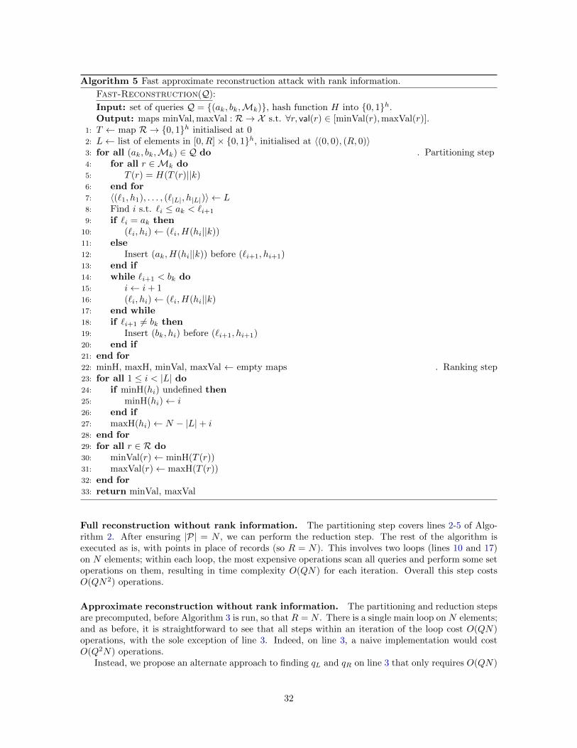
Algorithm 5 Fast approximate reconstruction attack with rank information.

Fast-Reconstruction(Q):

Input: set of queries Q = (ak, bk,Mk), hash function H into 0, 1h.Output: maps minVal,maxVal : R → X s.t. ∀r, val(r) ∈ [minVal(r),maxVal(r)].

1: T ← map R → 0, 1h initialised at 02: L← list of elements in [0, R]× 0, 1h, initialised at 〈(0, 0), (R, 0)〉3: for all (ak, bk,Mk) ∈ Q do . Partitioning step4: for all r ∈Mk do5: T (r) = H(T (r)||k)6: end for7: 〈(`1, h1), . . . , (`|L|, h|L|)〉 ← L8: Find i s.t. `i ≤ ak < `i+1

9: if `i = ak then10: (`i, hi)← (`i, H(hi||k))11: else12: Insert (ak, H(hi||k)) before (`i+1, hi+1)13: end if14: while `i+1 < bk do15: i← i+ 116: (`i, hi)← (`i, H(hi||k)17: end while18: if `i+1 6= bk then19: Insert (bk, hi) before (`i+1, hi+1)20: end if21: end for22: minH, maxH, minVal, maxVal ← empty maps . Ranking step23: for all 1 ≤ i < |L| do24: if minH(hi) undefined then25: minH(hi)← i26: end if27: maxH(hi)← N − |L|+ i28: end for29: for all r ∈ R do30: minVal(r)← minH(T (r))31: maxVal(r)← maxH(T (r))32: end for33: return minVal, maxVal

Full reconstruction without rank information. The partitioning step covers lines 2-5 of Algo-rithm 2. After ensuring |P| = N , we can perform the reduction step. The rest of the algorithm isexecuted as is, with points in place of records (so R = N). This involves two loops (lines 10 and 17)on N elements; within each loop, the most expensive operations scan all queries and perform some setoperations on them, resulting in time complexity O(QN) for each iteration. Overall this step costsO(QN2) operations.

Approximate reconstruction without rank information. The partitioning and reduction stepsare precomputed, before Algorithm 3 is run, so that R = N . There is a single main loop on N elements;and as before, it is straightforward to see that all steps within an iteration of the loop cost O(QN)operations, with the sole exception of line 3. Indeed, on line 3, a naive implementation would costO(Q2N) operations.

Instead, we propose an alternate approach to finding qL and qR on line 3 that only requires O(QN)

32

operations. Let Q denote the set of queries, where each query is identified with the set of matchedrecords. Let f(r) = q ∈ Q : M ⊆ q, r ∈ q, where M :=

⋂k:r∈MkMk is defined on line 2 of the

algorithm (note that M depends on r).For every record r, compute |f(r)| (by setting up an array of counters, one for each r, and scanning

once through every query, this costs O(QN) operations), and pick a record rL 6∈ M maximising thisvalue.16 Then pick qR of maximal size among queries such that M ⊆ qR and rL 6∈ qR. Then pickqL of maximal size among queries such that M ⊆ qL and qL ∩ qR = M . The time complexity of thisalgorithm is clearly O(QN) operations. We claim that it outputs the correct sets qL and qR expectedin line 3 of Algorithm 3.

To see this, switch the perspective from sets of records to the corresponding sets of values. Byconstruction M is an intersection of queries, so it covers an interval of values [xM , yM ]. Without lossof generality xL = val(rL) < xM . The crucial point is that by construction of rL, any query q ⊃ Mcontaining a record r with xL ≤ val(r) < xM must also contain rL: otherwise r would directly witnessthe fact that rL fails to maximise |f(r)| (indeed, by nature of intervals, any query containing M andrL must contain r, so |f(r)| ≥ |f(rL)|; but q belongs to f(r) and not f(rL) so the inequality is strict).Hence qR is the largest query containing M and not covering any value < xM ; likewise qL is the largestquery containing M and not covering any value > yM ; and we are done.

Overall complexity. In both cases the algorithms themselves cost O(QN2) operations, after thepartitioning and reduction steps, which cost O(Q(N+R)) operations. Hence the final tally is O(Q(N2+R)) operations.

B Upper Bounds on Data Complexity

In this section, we prove upper bounds on the expected number of queries necessary for Algorithms 1,2, and 3 to succeed. In each case a lower bound on the success probability of the algorithm (as afunction of the number of queries) is also provided. We begin with two useful lemmas.

B.1 Basic Distribution Lemmas

Recall that U denotes the uniform distribution on non-empty intervals in X = [1, N ].

Lemma 1. For all k ∈ [1, N ]:

Pr [x = k : [x, y]← U ] =2(N + 1− k)

N(N + 1)

Pr [y = k : [x, y]← U ] =2k

N(N + 1).

Proof. Since we allow singleton ranges, but not empty ones, there are N(N + 1)/2 choices for [x, y].Moreover for any k ∈ [1, N ], exactly N + 1 − k of those choices satisfy x = k (one for each choice ofy ≥ k). Hence the distribution of x for [x, y] ← U is as claimed. By the reflection symmetry of theproblem (flipping [1, N ], replacing k by N + 1− k) we get the second equality.

Lemma 2. Assume N is a multiple of 4. Suppose we have drawn Q ranges r = [x, y]← U . Let ELhalfdenote the event that there exist two ranges r, r′ such that r ∪ r′ = [1, N/2 + 1] and r ∩ r′ 6= ∅. LetERhalf denote the event that there exist two ranges r, r′ such that r∪ r′ = [N/2 + 1, N ] and r∩ r′ 6= ∅.17

Then:Pr[ELhalf

]≥ Pr

[ERhalf

]≥ 1− 2e−Q/(2N+2).

16The case M = R can be safely ignored, since it can only lead to a trivial approximate reconstruction.17There is a small asymmetry here: [1, N/2 + 1] covers N/2 + 1 values while [N/2 + 1, N ] covers N/2 values. This will

be helpful in the proof of Proposition 3.

33

Proof. Let us begin with ERhalf. Let ER1 denote the event that we have drawn a range r = [N/2 + 1, y]

for some y ∈ [3N/4 + 1, N ]. Let ER2 denote the event that we have drawn a range r′ = [x,N ] for somex ∈ [N/2 + 1, 3N/4]. If both ER1 and ER2 occur, then ERhalf clearly occurs.

There are N(N+1)/2 possible ranges, among which we draw uniformly at random. In the definitionof range r (resp. r′) for event ER1 (resp. ER2 ), there are N/4 choices for the value of x (resp. y). Itfollows that for a single draw:

Pr[ER1]

= Pr[ER2]

=N/4

N(N + 1)/2=

1

2(N + 1)

Hence after Q independent draws:

Pr[¬ER1

]= Pr

[¬ER2

]=

(1− 1

2(N + 1)

)Q= eQ ln(1− 1

2(N+1) )

≤ e−Q

2(N+1)

Hence we have:

Pr[ERhalf

]≥ Pr

[ER1 ∩ ER2

]≥ 1− Pr

[¬ER1

]− Pr

[¬ER2

]≥ 1− 2e−Q/(2N+2).

We now show Pr[ELhalf

]≥ Pr

[ERhalf

]. By symmetry, the probability of the event E′: there exist

r, r′ such that r ∪ r′ = [1, N/2] and r ∩ r′ 6= ∅, is equal to ERhalf. Thus it suffices to show that this

event is less likely than ELhalf. To see this, let f denote the permutation on ranges in [1, N ] defined by:

f([x, y]) =

[x,N/2 + 1] if y = N/2;

[x,N/2] if y = N/2 + 1 and x ≤ N/2;

[x, y] otherwise.

The point of f is that it maps any pair of ranges r, r′ witnessing E′ into a pair witnessing ELhalf (theconverse is not true, as shown by the pair [1, N/2 + 1], [N/2 + 1, N/2 + 1]). As a consequence, if weconsider sequences of Q queries, then if some sequence Q satisfies E′ we have that f(Q) satisfies ELhalf.

Since f is a permutation, this shows that the number of sequences of queries satisfying ELhalf is higherthan the number of sequences of queries satisfying E′. Because we are working with the uniformdistribution, this implies:

Pr[ELhalf

]≥ Pr [E′] = Pr

[ERhalf

].

B.2 Upper Bound for the Full Reconstruction Attack with Rank

Proposition 1. Assume N is a multiple of 4. Assume that the database is dense, and range queriesare drawn uniformly at random. Then the probability of success of Algorithm 1 after Q queries islower-bounded by:

1− 2e−Q/(2N+2) −Ne−Q/N .

Moreover, the expected number of queries before the algorithm succeeds is upper-bounded by:

N log(N) +O(N).

Concretely, for N ≥ 27, it is upper-bounded by N(log(N) + 1) + 4.4√N + 4 ≤ N(log(N) + 2).

34

Proof. Let Q = qk = (ak, bk,Mk) : k ≤ Q denote the set of queries. For each k ≤ Q, let [xk, yk] ⊆[1, N ] denote the range of values on which the k-th query qk bears, i.e. Mk = r ∈ R : val(r) ∈[xk, yk]. From the discussion in Section 2.3, recall that Algorithm 1 succeeds iff the partition of valuesV contains N elements. It is easy to see that this is equivalent to the condition that for all v ∈ [1, N ],I(v) = v, where I(v) is defined by:

I(v) =⋂

v∈[xk,yk]

[xk, yk] \

⋃v 6∈[xk,yk]

[xk, yk]

. (5)

In other words, Algorithm 1 succeeds iff the following event occurs:

E = [∀v ∈ [1, N ], v = I(v)].

Our goal in this proof is to lower-bound the probability of E as a function of the number Q of queries.For this purpose, we split E into a a set of simpler events whose joint occurrence implies E.

First, we define event ERhalf: there exist two queries qk, qk′ such that [xk, yk]∪[xk′ , yk′ ] = [N/2+1, N ].

Lemma 2 provides a lower bound for the probability of this event.18 In addition, we define events ELx :there exists a query with left end point x; and ERy : there exists a query with right end point y.

By analogy to the coupon collector’s problem, we call ELx a left coupon, and ERy a right coupon.The idea is that if we collect all left coupons in [1, N/2] and all right coupons in [N/2 + 1, N ], inaddition to ERhalf, then E happens and the algorithm succeeds. This is expressed by the followingclaim.

Claim 1.

E ⊇ ERhalf ∩

N/2⋂x=1

ELx

∩ N⋂y=N/2+1

ERy

.

Proof. Pick v ∈ [1, N ]. Assume v ≤ N/2. The proof for v > N/2 is similar. From the definitionof I(v), it is clear that v ∈ I(v). Conversely, let w ∈ [1, N ] \ v. We want to show w 6∈ I(v). Wedistinguish three cases.

1. If w < v, ELv implies w 6∈ I(v) as w cannot belong to the intersection on the left side of (5).

2. If w ∈ [v + 1, N/2], ELw implies w 6∈ I(v) as w must belong to the union on the right side of (5).

3. If w ∈ [N/2 + 1, N ], ERhalf implies w 6∈ I(v) as w must belong to the union on the right side of(5).

A small subtlety worth pointing out is that for the case v > N/2, the third case becomes w ∈ [1, N/2],and ERhalf is sufficient to handle it as it implies that the intersection on the left side of (5) must be

contained in [N/2 + 1, N ]. As a result the reflection ELhalf of ERhalf is not needed in this proof.

It now remains to lower-bound the probability of⋂N/2x=1E

Lx and

⋂Ny=N/2+1E

Ry . Note that these

two events are completely symmetric via the reflection that flips [1, N ], replacing k by N + 1− k andswitching the roles of left and right coupons. In particular the two aforementioned events must have

18There are two small abuses of notation: first, in Lemma 2, ERhalf was an event on ranges, whereas here ER

half is an

event on queries; in this case we assimilate a query with the corresponding queried range. Second, the event ERhalf as

defined in Lemma 2 also requires [xk, yk] ∩ [xk′ , yk′ ] 6= ∅, so it is a strict subset of ERhalf as defined here, but since it is

used as a lower bound this works to our advantage.

35

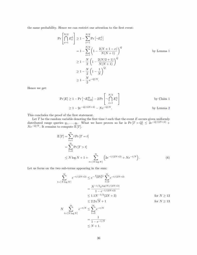
the same probability. Hence we can restrict our attention to the first event:

Pr

N/2⋂x=1

ELx

≥ 1−N/2∑x=1

Pr[¬ELx

]

= 1−N/2∑x=1

(1− 2(N + 1− x)

N(N + 1)

)Qby Lemma 1

≥ 1− N

2

(1− 2(N/2 + 1)

N(N + 1)

)Q≥ 1− N

2

(1− 1

N

)Q≥ 1− N

2e−Q/N .

Hence we get:

Pr [E] ≥ 1− Pr[¬ERhalf

]− 2 Pr

¬N/2⋂x=1

ELx

by Claim 1

≥ 1− 2e−Q/(2N+2) −Ne−Q/N . by Lemma 2

This concludes the proof of the first statement.Let T be the random variable denoting the first time t such that the event E occurs given uniformly

distributed range queries q1, . . . , qt. What we have proven so far is Pr [T > Q] ≤ 2e−Q/(2N+2) +Ne−Q/N . It remains to compute E [T ].

E [T ] =

∞∑t=1

tPr [T = t]

=

∞∑t=0

Pr [T > t]

≤ N logN + 1 +

∞∑t=dN logNe

(2e−t/(2N+2) +Ne−t/N

). (6)

Let us focus on the two sub-terms appearing in the sum:

∞∑t=dN logNe

e−t/(2N+2) ≤ e−N log(N)2N+2

∞∑t=0

e−t/(2N+2)

=N−1/2elog(N)/(2N+2)

1− e−1/(2N+2)

≤ 1.1N−1/2(2N + 3) for N ≥ 13

≤ 2.2√N + 1 for N ≥ 13

N

∞∑t=dN logNe

e−t/N ≤∞∑t=0

e−t/N

=1

1− e−1/N

≤ N + 1.

36

where lines 3 and 7 use the fact that 1/(1− e−1/x) ≤ 1 + x for x ≥ 0.Reinjecting into (6), we conclude that for N ≥ 13:

E [T ] ≤ N log(N) +N + 4.4√N + 4.

For N ≥ 27, 4.4√N + 4 ≤ N so in that case we have:

E [T ] ≤ N(log(N) + 2).

B.3 Upper Bound for the Full Reconstruction Attack Without Rank

Proposition 2. Assume N is a multiple of 4. Assume that the database is dense, and range queriesare drawn uniformly at random. Then the probability of success of Algorithm 2 after Q queries islower-bounded by:

1− 4e−Q/(2N+2) −Ne−Q/(N+1).

Moreover, the expected number of queries before the algorithm succeeds is upper-bounded by:

N log(N) +O(N).

Concretely, for N ≥ 26, it is upper-bounded by (N + 1)(log(N) + 1) + 8√N + 6 ≤ N(log(N) + 3).

Proof. Let Q = qk = (Mk) : k ≤ Q denote the set of queries. For each k ≤ Q, let [xk, yk] ⊆ [1, N ]denote the range of values on which the k-th query qk bears, i.e. Mk = r ∈ R : val(r) ∈ [xk, yk].

The proof closely follows the case where rank information is available. Let E denote the eventthat Algorithm 2 succeeds. We are going to define several events whose joint occurrence implies E.In fact, these events will be almost the same as those of Proposition 1. Then in a second step we willlower-bound the probability of these events.

Define event ERhalf: there exist two queries qk, qk′ such that [xk, yk] ∪ [xk′ , yk′ ] = [N/2 + 1, N ]

and [xk, yk] ∩ [xk′ , yk′ ] 6= ∅. Likewise, define event ELhalf: there exist two queries qk, qk′ such that

[xk, yk] ∪ [xk′ , yk′ ] = [1, N/2] and [xk, yk] ∩ [xk′ , yk′ ] 6= ∅. Next, we define events E′Lx : there exists aquery qk with left end point xk = x and length at least 2 (i.e. yk − xk + 1 ≥ 2). Likewise, let E′Rydenote the event: there exists a query with right end point y and length at least 2 (in the same sense).Thus the definition of ERhalf matches that of Lemma 2, and ELhalf is its reflection; while E′Lx and E′Ryare identical to ELx and ERy from Proposition 1, except for the additional requirement that queriesshould have length at least 2.

We call E′Lx a left coupon, and E′Ry a right coupon. The idea is that if we collect all left coupons

in [1, N/2] and all right coupons in [N/2 + 1, N ], in addition to ELhalf and ERhalf, then E happens andthe algorithm succeeds. This is expressed by the following claim (which is of course the counterpartof Claim 1).

Claim 2.

E ⊇ ELhalf ∩ ERhalf ∩

N/2⋂x=1

E′Lx

∩ N⋂y=N/2+1

E′Ry

.

Proof. Throughout, we assume that events ELhalf, ERhalf,

⋂N/2x=1E

Lx and

⋂Ny=N/2+1E

Ry occur. Our goal

is to show that E happens, i.e. Algorithm 2 succeeds. There are three lines where Algorithm 2 canfail: lines 7, 14, and 24. We examine each of them in turn.

First, notice that the first fail condition on line 7 in Algorithm 2 is exactly equivalent to thefail condition on line 7 in Algorithm 1. Moreover the events E′Lx , E′Ry are strict subsets of their

counterparts ELx , ERy in Claim 1 from the proof of Proposition 1 (and so is ERhalf). By Claim 1, itfollows that Algorithm 1 cannot fail, and hence Algorithm 2 also cannot fail at line 7.

We now turn our attention to line 14. At this step the set of records has successfully been partitionedinto N subsets, contained in partition P. Each element of P is the set of records corresponding to a

37

particular value in [1, N ]. We call the elements of P points. The remainder of the algorithm is aimingto sort the set P of points according to their value. To start with, it is attempting to find an extremalpoint. To do so, it starts with an arbitrary query corresponding to some range [x, y] ( [1, N ], andprogressively extends it using the following process.

At each iteration the variable S holds a set of records corresponding to some interval [x, y] ( [1, N ]of values. Then it looks for a query q overlapping S and such that S ∪ q is not the full set R, and addsq to S. Iterations continue until no such q exists. The fail condition on line 14 is triggered iff at theend of this process, R \ S is not reduced to a single point. We now show that this is impossible.

Let [x, y] denote the interval of values corresponding to S. By construction there cannot exist qsuch that q overlaps S and q ∪ S 6= R. First, we show that x > 2 is impossible. Indeed in that case,if x ≤ N/2 + 1 (resp. x > N/2 + 1) then E′Lx−1 (resp. ERhalf) would yield a suitable q and hence acontradiction. So x ∈ [1, 2]. Similarly it must hold that y ∈ [N − 1, N ]. Moreover by construction ofS, [x, y] = [1, N ] is impossible, and [x, y] = [2, N − 1] is also impossible as ERhalf would yield a suitableq. We conclude that [x, y] = [2, N ] or [1, N − 1], and so R \ S must be reduced to a single point.

It remains to consider line 24. At this step of the algorithm, a loop invariant is that the variableI(i) holds the set of records whose value lies in [1, i], i.e. I(i) = S[1,i]. At iteration i, Q′ is the set ofall queries q overlapping I(i) such that q \ I(i) is non-empty, and T is the intersection of all queries inQ′ minus I(i). An invariant of the loop at line 20 is that T = S[i+1,j] for some j. The algorithm keepssubtracting queries q overlapping T as long as T remains non-empty, and q \ (T ∪ I(i)) 6= ∅. The failcondition at line 24 is triggered iff at the end of this process, the value interval [i+ 1, j] correspondingto records in T is not limited to a single point. We now show that this is impossible.

Indeed, if i < N/2, then j > N/2 is impossible as ELhalf provides a pair of queries covering all values

[1, N/2], so that the intersection of queries in Q′ must be contained in ELhalf; and N/2 ≥ j > i + 1

is likewise impossible as the query witnessing E′Lj would be subtracted from T during the subsequentloop at line 20. It follows that values covered by T are eventually reduced to i + 1. On the otherhand if i ≥ N/2, then E′Ri+1 provides a query q′ ∈ Q′ corresponding to an interval of values of the form[h, i+ 1] for some h ≤ i, so the initial value of the set T as the intersection of queries in Q′ is alreadyreduced to the single point Si+1.

It now remains to lower-bound the probability of⋂N/2x=1E

′Lx and

⋂Ny=N/2+1E

′Ry . As was the case

in the proof of Proposition 1, these two events are completely symmetric via the reflection that flips[1, N ], replacing k by N +1−k and switching the roles of left and right coupons. In particular the two

aforementioned events must have the same probability, and we shall limit our attention to⋂N/2x=1E

′Lx .

First, observe that there are exactly N − k possible ranges [k, y] ⊆ [1, N ] with left end point k andlength at least 2. It follows that after drawing a single uniformly random query, we have:

Pr[E′Lx

]=

2(N − x)

N(N + 1)

and after Q queries:

Pr[¬E′Lx

]=

(1− 2(N − x)

N(N + 1)

)Q. (7)

38

We have:

Pr

N/2⋂x=1

E′Lx

≥ 1−N/2∑x=1

Pr[¬E′Lx

]

= 1−N/2∑x=1

(1− 2(N − x)

N(N + 1)

)Qby (7)

≥ 1− N

2

(1− 1

N + 1

)Q≥ 1− N

2e−Q/(N+1).

Hence we get:

Pr [E] ≥ 1− 2 Pr[¬ERhalf

]− 2 Pr

¬N/2⋂x=1

E′Lx

by Claim 2

≥ 1− 4e−Q/(2N+2) −Ne−Q/(N+1). by Lemma 2

This concludes the proof of the first statement.Let T be the random variable denoting the first time t such that the event E occurs given uniformly

distributed range queries q1, . . . , qt. What we have proven so far is Pr [T > Q] ≤ 4e−Q/(2N+2) +Ne−Q/(N+1). It remains to compute E [T ].

E [T ] =

∞∑t=0

Pr [T > t]

≤ (N + 1) logN + 1 +

∞∑t=d(N+1) logNe

(4e−t/(2N+2) +Ne−t/(N+1)

). (8)

Let us focus on the two sub-terms appearing in the sum:

∞∑t=d(N+1) logNe

e−t/(2N+2) ≤ 1√N

∞∑t=0

e−t/(2N+2)

=1/√N

1− e−1/(2N+2)

≤ 1√N

(2N + 3)

≤ 2√N + 1 for N ≥ 9

N

∞∑t=d(N+1) logNe

e−t/(N+1) ≤∞∑t=0

e−t/(N+1)

=1

1− e−1/(N+1)

≤ N + 2.

where lines 3 and 7 use the fact that 1/(1− e−1/x) ≤ 1 + x for x ≥ 0.Reinjecting into (8), we conclude that for N ≥ 9:

E [T ] ≤ (N + 1) log(N) +N + 8√N + 7.

For N ≥ 26, 8√N + log(N) + 7 ≤ 2N so in that case we have:

E [T ] ≤ N(log(N) + 3).

39

B.4 Upper Bound for the Approximate Reconstruction Attack

Proposition 3. Assume N is a multiple of 4, εN/2 is an integer, and ε < 3/4. Assume that thedatabase is dense, and range queries are drawn uniformly at random. Then the probability of successof Algorithm 3 after Q queries is lower-bounded by:

1− 4e−Q/(2N+2) − 2e−Q log(1+ε/2)+εN/2·(log(1/ε)+1.5).

Moreover, the expected number of queries before the algorithm succeeds is upper-bounded by:

5

4N log(1/ε) +O(N).

Concretely, for N ≥ 40, it is upper-bounded by (1 + ε/4)N log(1/ε) + (2 + 4√ε)N + 4/ε.

Proof. Let Q = qk = (Mk) : k ≤ Q denote the set of queries. For each k ≤ Q, let [xk, yk] ⊆ [1, N ]denote the range of values on which the k-th query qk bears, i.e. Mk = r ∈ R : val(r) ∈ [xk, yk].

The proof follows the outline of the proofs of Propositions 1 and 2. Let E denote the event thatAlgorithm 3 succeeds. We are going to define several events whose joint occurrence implies E. Theseevents will be similar to those used in the proofs of Propositions 1 and 2. Then in a second step wewill lower-bound their joint probability.

Define the following events:

- ELhalf: there exist two queries qk, qk′ such that [xk, yk] ∪ [xk′ , yk′ ] = [1, N/2 + 1] and [xk, yk] ∩[xk′ , yk′ ] 6= ∅.

- ERhalf: there exist two queries qk, qk′ such that [xk, yk] ∪ [xk′ , yk′ ] = [N/2 + 1, N ] and [xk, yk] ∩[xk′ , yk′ ] 6= ∅.

- E′′Lx : there exists a query qk with xk = x ≤ N/2 and yk > N/2.

- E′′Ry : there exists a query qk with xk ≤ N/2 and yk = y > N/2.

As in previous proofs, we call E′′Lx a left coupon, and E′′Ry a right coupon. The idea is that if wecollect (1 − ε)N/2 left coupons in [1, N/2] and (1 − ε)N/2 right coupons in [N/2 + 1, N ], in additionto ELhalf and ERhalf, then the algorithm succeeds. This is expressed by the following claim.

Claim 3. Let CL (resp. CR) denote the event that there exist (1 − ε)N/2 distinct values x ≤ N/2(resp. y > N/2) such that E′′Lx (resp. E′′Ry ) occurs. Then:

E ⊇ ELhalf ∩ ERhalf ∩ CL ∩ CR.

Proof. Throughout, we assume that events ELhalf, ERhalf, CL, and CR occur. Our goal is to show that

E happens, i.e. Algorithm 3 succeeds. This is rather straightforward, as the algorithm is designedprecisely to take advantage of the aforementioned events.

Algorithm 3 can only fail at line 30, if no suitable record r was found during the course of the mainloop. Let r now denote any record with value N/2 + 1. We claim that the algorithm must succeed forthis particular choice of r, and hence the fail condition at line 30 is never triggered.

We now show that the algorithm succeeds for r such that val(r) = N/2 + 1. First, ELhalf ∩ ERhalfimplies that the variable M at line 2 is reduced to the set SN/2+1 of records with value N/2 + 1. Theevent ELhalf∩ERhalf also implies that the test on line 6 is satisfied. Then CL implies that nL ≥ (1−ε)N/2.Likewise CR implies nR ≥ (1 − ε)N/2 − 1; the minus 1 in the last expression is due to the fact thevalue N/2+1 may account for one of the right coupons, whereas sets in R\halfL contain records withvalues in [N/2 + 2, N ] (as M is excluded). Thus nL + nR + 1 ≥ (1 + ε)N , so the test at line 15 is alsosatisfied, which means that the algorithm has succeeded in finding a solution.

40

It now remains to study the probability of CL and CR. As was the case in the proofs of Proposi-tions 1 and 2, these two events are symmetric and hence must have the same probability, so we focuson CL.

Let Tk denote the random variable such that the k-th distinct left coupon in [1, N/2] is collected attime Tk, with the convention T0 = 0. Let ∆k = Tk+1 − Tk. Notice that CL happens iff T(1−ε)N/2 ≤ Q.To simplify notation we will write T(1−ε)N/2 simply as T .

Suppose k left coupons have been collected for some k ≥ 0. Then there are (N/2− k) ·N/2 rangesin [1, N ] that constitute a new left coupon. Hence the probability of drawing a new left coupon is:

pk :=(N/2− k) ·N/2N(N + 1)/2

=N/2− kN + 1

.

The variable ∆k follows a geometric distribution with probability pk.We wish to upper-bound the probability of the event ¬CL, which is equivalent to T > Q. For this

purpose we note that T is a sum of the independent variables ∆k, and use the Chernoff bound:

Pr [T > Q] ≤ e−xQ(1−ε)N/2−1∏

k=0

E[ex∆k

](9)

for any x > 0 (which we will soon choose). Since the ∆k’s are geometrically distributed with probabilitypk, their moment-generating function E

[ex∆k

]satisfies:

E[ex∆k

]=

pkex

1− (1− pk)ex

with the constraint ex < 1/(1 − pk). The most demanding constraint arises for k = (1 − ε)N/2 − 1,namely:

ex <1

1− p(1−ε)N/2−1

=N + 1

(1− ε/2)N.

We set x = log(1 + ε/2),19 which is easily verified to satisfy that constraint; indeed:

(1− ε/2)ex = 1− ε2/4 < (N + 1)/N.

Reinjecting into the Chernoff bound (9) gives:

Pr [¬CL] ≤ e−(Q−(1−ε)N/2)x

(1−ε)N/2−1∏k=0

pk1− (1− pk)ex

. (10)

We now focus on the product P appearing on the right-hand side of the previous equation:

P :=

(1−ε)N/2−1∏k=0

pk1− (1− pk)(1 + ε/2)

=

(1−ε)N/2−1∏k=0

(1− ε

2

(1

pk− 1

))−1

=

(1−ε)N/2−1∏k=0

(1− ε

2

(N/2 + k + 1

N/2− k

))−1

.

19To shed some light into the choice of x: we want x to be “large” since it dictates the rate of exponential decreasein the bound, but ex has to be strictly lower than 1/(1 − ε/2) · (N + 1)/N . The idea is that the term 1/(1 − ε/2)is the important one (the other term would essentially disappear if we were to collect even one more coupon), andex = 1 + ε/2 is a first-order approximation of this upper bound, which conveniently happens to be lower than it since1/(1− ε/2) = 1 + ε/2 + ε2/4 + . . .

41

In this formula, as one would expect, the highest contributing terms occur as k gets close to its upperbound (as collecting the last coupons is more expensive than the first). Before continuing, we performthe change of variables s := (1 − ε)N/2 − k, which sends the most significant terms to s = 0, 1, 2, . . .(and, in our view, improves the readability of the formula).

P =

(1−ε)N/2∏s=1

(1− ε

2

(N − εN/2− s+ 1

εN/2 + s

))−1

=

(1−ε)N/2∏s=1

(ε

2+

s− ε/2s+ εN/2

)−1

log(P ) =

(1−ε)N/2∑s=1

− log

(ε

2+

s− ε/2s+ εN/2

)

≤∫ (1−ε)N/2

s=0

− log

(ε

2+

s− ε/2s+ εN/2

). (11)

Note that the logarithm remains well-defined thanks to the assumption ε ≥ 2/N . It is straightforwardto check that a primitive integral of the above function may be written as F1(s) +F2(s) +F3(s) with:

F1(s) = −s log

(ε

2+

s− ε/2s+ εN/2

)F2(s) =

εN

2log

(s+

εN

2

)F3(s) =−ε/2(Nε/2− 1)

1 + ε/2log

(s+

ε/2(Nε/2− 1)

1 + ε/2

).

Let us start with the contribution of F1:

F1((1− ε)N/2)− F1(0) = − (1− ε)N2

log

(1− ε

(1

2+

1

N

))≤ εN

2(1− ε)

(1 +

2

N

)≤ εN

2

(1 +

2

N− ε− Nε

2

)≤ εN

2(12)

where the second line uses − log(1− t) < 2t for t < 3/4 (recall ε < 3/4 is an assumption); and the lastline uses ε ≥ 2/N . We turn to F2 and F3:

F2((1− ε)N/2)− F2(0) =εN

2log

(1

ε

)(13)

F3((1− ε)N/2)− F3(0) = −ε/2(Nε/2− 1)

1 + ε/2log

(1 + (1− ε)

(1 +

ε

2

) N2

).

The contribution of F3 is clearly negative; since we are trying to upper-bound P , we discard it.Reinjecting (12) and (13) into (11) leaves us with:

log(P ) ≤ εN

2

(log

(1

ε

)+ 1

).

Finally, reinjecting this last inequality into (10) gives:

log (Pr [¬CL]) ≤ −Q log(

1 +ε

2

)+

(1− ε)N2

log(

1 +ε

2

)+εN

2

(log

(1

ε

)+ 1

).

42

Using log(1 + x) ≤ x we can upper-bound the middle summand by εN/4, which simplifies the boundinto:

log (Pr [¬CL]) ≤ −Q log(

1 +ε

2

)+εN

2

(log

(1

ε

)+ 1.5

).

Combining this last inequality with Lemma 2 yields the desired result:

Pr [E] ≥ 1− 2 Pr[¬ERhalf

]− 2 Pr [¬CL]

≥ 1− 4e−Q/(2N+2) − 2e−Q log(1+ε/2)+εN/2·(log(1/ε)+1.5).

This concludes the proof of the first statement.Let T ′ be the random variable denoting the first time t such that the event E occurs given uniformly

distributed range queries q1, . . . , qt. What we have proven so far is:

Pr [T ′ > Q] ≤ 4e−Q/(2N+2) + 2e−Q log(1+ε/2)+εN/2·(log(1/ε)+1.5). (14)

It remains to compute E [T ′]. Let us define:

s :=ε/2

log(1 + ε/2)N(log(1/ε) + 1.5).

Thus, s is chosen so that setting Q = s cancels the exponent in the second (and dominant) term in(14). We have:

E [T ′] =

∞∑t=0

Pr [T ′ > t]

≤ s+ 1 +

∞∑t=dse

(4e−Q/(2N+2) + 2e−Q log(1+ε/2)+εN/2·(log(1/ε)+1.5)

). (15)

Let us focus on the two sub-terms appearing in the sum:∞∑

t=dse

e−t/(2N+2) ≤ e−N

2N+2 (log(1/ε)+1.5)∞∑t=0

e−t/(2N+2)

=

√ε · e− 3

4 +(log(1/ε)/2+ 34 )/(N+1)

1− e−1/(2N+2)

≤ 1

2

√ε(2N + 3) for N ≥ 39

∞∑t=dse

e−t log(1+ε/2)+εN/2·(log(1/ε)+1.5) ≤∞∑t=0

e−t log(1+ε/2)

=1

1− (1 + ε/2)−1

=2

ε+ 1.

where the first line uses x/ log(1 + x) ≥ 1, and line 3 uses 1/(1− e−1/x) ≤ 1 + x for x ≥ 0, as well asε ≥ 2/N .

Reinjecting into (15), we conclude that for N ≥ 39:

E [T ′] ≤ ε/2

log(1 + ε/2)N(log(1/ε) + 1.5) +

√ε(4N + 6) +

4

ε+ 3.

Using the fact x/(log(1 + x)) ≤ 1 + x/2 for x ≥ 0, and ε < 1, we get the desired result:

E [T ′] ≤ (1 + ε/4)N(log(1/ε) + 1.5) + 4√εN + 4/ε+ 9

≤ (1 + ε/4)N log(1/ε) + (2 + 4√ε)N + 4/ε

where the last line uses N ≥ 40 and ε < 3/4.

43

C Lower Bounds on Data Complexity

Let Q = (Mk) denote a set of queries. Rank information will play no role in this section, and ourresults hold with or without it. Recall from Section 2.3 that the partition of records P = P (r) : r ∈ Ris defined by:

P (r) =

( ⋂k:r∈Mk

Mk

)∖( ⋃k:r 6∈Mk

Mk

).

Likewise, the partition of values V = V (r) : r ∈ R is defined by:

V (r) =

( ⋂k:r∈Mk

[xk, yk]

)∖( ⋃r 6∈Mk

[xk, yk]

).

Also recall that there is a one-to-one correspondence between P and V (induced by val). In particular|P| = |V|.

The number k = |P| ≤ N plays a crucial role: any algorithm operating on Q can only meaningfullyseparate k distinct classes among records. Intuitively, it is clear that such an algorithm can only assignvalues to records up to a precision of N − k. In this section, we lower-bound the expected numberof queries required to reach a given threshold |P| ≥ k. We then formalise the previous intuition todeduce a lower bound on the expected number of queries necessary to assign values to records withprecision of N − k.

Proposition 4. Let P denote the partition of records induced by a set of uniformly random rangequeries. Let k ≤ N . Then the expected number of queries necessary to attain |P| ≥ k is lower-boundedby:

1

2N log

(N + 1

N + 2− k

)− 1

2.

Proof. As already noted, the partition of values is in bijection with the partition of records. In thisproof we focus on the partition of values. When a range query is issued on some range [x, y] ⊆ [1, N ],this query potentially allows to separate values below or above x, and below or above y. Followingthis observation, let us define S = [0, N ] as the set of separators. We say that a range [x, y] yields theseparators x− 1 and y. The idea is that a separator s ∈ S allows to separate values ≤ s and > s.

The set of all records is assumed to be known. Since we are looking to lower-bound the requirednumber of queries necessary for an attack, this is a fair assumption (we are assuming more informationis available). As a result, the separators 0 and N bring no information, and we assume they are knownfrom the start. Define inner separators as separators in [1, N − 1]. The crucial point is that if we havecollected k distinct inner separators, then we are able to partition the values [1, N ] into at most k+ 1sub-intervals. Indeed, we start knowing 1 interval of values, namely [1, N ]; and each new, distinctinner separator splits the interval in which it falls in two.

Hence, in order to lower-bound the expected number of queries required to reach |P| ≥ k, it sufficesto lower-bound the number of queries necessary to collect k−1 distinct inner separators. This is anothervariant of the coupon collector’s problem, viewing inner separators as coupons. In the remainder wewill use the terms inner separator and coupon interchangeably. Our goal is to lower-bound the numberof trials necessary to collect k − 1 coupons (among N − 1 possible coupons). Each trial consists indrawing a uniform range [x, y] ⊆ [1, N ] and collecting the coupon(s) x− 1, y \ 0, N.

The distribution of each trial can be characterised as follows. Note that there are M = N(N+1)/2choices of [x, y]. Let S ⊆ [1, N − 1] be a set of coupons of size at most two. Then the probability thatwe collect exactly S during a given trial is:

• p0 = 1/M if |S| = 0: indeed this occurs iff [x, y] = [1, N ];

• p1 = 2/M if |S| = 1: indeed letting S = s, this occurs iff [x, y] = [1, s] or [x, y] = [s+ 1, N ];

• p2 = 1/M if |S| = 2: indeed letting S = s, t, this occurs iff [x, y] = [s+ 1, t].

44

Let us denote by D the above distribution (on subsets of coupons of size at most two).On the other hand, let D′ denote the distribution induced by drawing two coupons independently

and uniformly at random, and taking their union. Note that there are M ′ = (N − 1)2 possible pairsof coupons. For S ⊆ [1, N − 1] of size at most 2, the probability of drawing S for this new distributionis defined by:

• p′0 = 0 if |S| = 0;

• p′1 = 1/M ′ if |S| = 1: indeed letting S = s, this occurs iff we draw the pair (s, s);

• p′2 = 2/M ′ if |S| = 2: indeed letting S = s, t, this occurs iff we draw the pair (s, t) or (t, s).

The point of D′ is that it amounts to a sequence of two trials in the standard coupon collector’sproblem with a uniform distribution. On the other hand, the following claim shows that, for ourpurpose, we can effectively replace D by the much more agreeable D′.

Claim 4. Let TDk (resp. TD′

k ) denote the number of trials until k coupons have been collected with

distribution D (resp. D′). Then E[TDk]≥ E

[TD

′

k

].

Proof. Let C denote the set of subsets of coupons of size at most two (so that D and D′ are distributionson C). Define the probabilistic mapping f : C → C by:

f(S) = S′ where

if S = ∅, draw S′ ← D′;

if S = s

with probability N+2

4(N−1) set S′ = S;

otherwise S′ = s, t with t$←− [1, N − 1] \ s;

if S = s, t, set S′ = S.

We claim that f sends the distribution D to D′. To see this, it suffices to check that D′ and f(D) matchon subsets of size 0 and 1. Indeed, both are probability distributions, and are uniform among subsetsof a given size. Both distributions assign probability 0 to the empty set. As for a given singleton s,D′ assigns probability 1/(N − 1)2 and f(D) assigns:

p0p′1 + p1

N + 2

4(N − 1)=

2

N(N + 1)· 1

(N − 1)2+

4

N(N + 1)· N + 2

4(N − 1)

=1

(N − 1)2.

Moreover f is designed in such a way that it can only add new coupons. It follows that the expectednumber of trials to collect k coupons is lower with distribution f(D) = D′ than with distribution D.

Claim 5.

E[TD

′

k

]≥ N

2log

(N + 1

N + 1− k

)− 1

2.

Proof. As noted earlier, a single trial with distribution D′ is equivalent to two trials in a standardcoupon collector’s problem with uniform distribution. Let Uk be the number of trials after which kdistinct coupons have been collected in a standard coupon collector’s problem with N − 1 elements.

45

From this perspective:

E[TD

′

k

]=

∞∑t=0

tPr [(Uk = 2t) ∪ (Uk = 2t+ 1)]

=1

2

∞∑t=0

2t (Pr [Uk = 2t] + Pr [Uk = 2t+ 1])

=1

2

∞∑t=0

(2tPr [Uk = 2t] + (2t+ 1) Pr [Uk = 2t+ 1]

)− 1

2

∞∑t=0

Pr [Uk = 2t+ 1]

≥ 1

2

∞∑t=0

tPr [Uk = t]− 1

2

∞∑t=0

Pr [Uk = t]

=1

2(E [Uk]− 1). (16)

On the other hand, by standard arguments:

E [Uk] = N(HN −HN−k)

= N

N∑i=N−k+1

1

i

≥ N∫ N+1

x=N−k+1

1

x

= N(log(N + 1)− log(N + 1− k)).

Combining this with (16) yields the result.

Summing up, we have shown that |P| ≥ k implies we have collected at least k− 1 inner separators,so the expected number of queries to reach |P| ≥ k is lower-bounded by E

[TDk−1

]. By Claim 4 this

expectation is itself lower-bounded by E[TD

′

k−1

], and Claim 5 yields the result.

Proposition 5. Let A denote any (computationally unbounded) adversary observing the leakage ofa sequence of uniformly random range queries (including rank information). In addition to queryleakage, A takes as input a quantity 0 < ε < 1. A outputs either ⊥ (fail), or correctly assigns to allrecords r an interval of values containing val(r) of length at most εN (success). Then the expectednumber of queries that A must observe before it succeeds is lower-bounded by:

1

2N log

(N + 1

εN + 2

)− 1

2=

1

2N log

(1

ε

)−O(N).

Proof. By Proposition 4, it suffices to show that if the partition of records P has cardinality less than(1− ε)N , then it is impossible to assign values to records with precision εN . To see this, define:

m : P → [1, N ]

p 7→ min(val(r) : r ∈ p).

Note that m is injective and order P by increasing value of m as p1, . . . , pP , where P = |P|. Define thetwo value assignments v, v′ : P → X characterised respectively by v(pi) = i, and v′(pi) = N−P+i.The crucial point is that, given the same range queries, v and v′ both leave the leakage observed bythe adversary unchanged. Hence the adversary cannot distinguish between these two assignments (or

46

the real assignment val, for that matter), and so it cannot determine (with probability 1) a range ofvalues for a given record with length strictly less than N − P .

Thus, in order for the adversary to be able to assign a range of length at most εN to all records,it must hold that P ≥ (1− ε)N . Whence Proposition 4 yields a lower bound on the expected numberof queries:

1

2N log

(N + 1

εN + 2

)− 1

2=

1

2

(N log

(1

ε

)+N log

(εN + ε

εN + 2

)− 1

)≥ 1

2

(N log

(1

ε

)−N log(3)− 1

)=

1

2N log

(1

ε

)−O(N).

where the inequality in the second line uses εN ≥ 1.

Corollary 1. If the adversary A of Proposition 5 wishes to correctly determine the value of all records,then the expected number of queries it must observe is lower-bounded by:

1

2N log

(N + 1

3

)− 1

2=

1

2N log(N)−O(N).

Proof. Set ε = 1/N in Proposition 5.

Remark 1. Obviously the lower bounds of Proposition 5 and Corollary 1 also hold for adver-saries that do not have access to rank information, since in that case the adversary has strictly lessinformation.

Remark 2. The results of Proposition 5 and Corollary 1 do not require that the database be dense,and known to be dense by the adversary. However the same results can be easily adapted to the casewhere the database is known to be dense e.g. by adding the assumption that at least two distinctvalues are taken by at least N records. This gives us enough leeway to “shift” the set of possible valuesbetween these two sets as in the proof of Proposition 5, while maintaining density.

D Data Optimality

We consider algorithms observing the leakage of a sequence of queries, with some specific statedobjective; and we restrict our attention to algorithms that are correct in the following sense: onany given input, either the algorithm fails, or its output correctly fulfills the stated objective withprobability 1. In this context, we say that an algorithm is data-optimal iff whenever the algorithmfails on a given input, then it was impossible to fulfill the stated objective given that input froman information theoretic perspective: i.e. no (computationally unbounded) correct algorithm giventhe same input would succeed in reaching the stated objective. Informally, a data-optimal algorithmconsumes the minimal amount of data required to reach its stated objective with probability 1, inessentially the strongest possible sense.

In this section, we prove that both our algorithms for full reconstruction,20 namely Algorithms 1and 2, are data-optimal in this strong sense. It is worth pointing out that computationally unboundeddata-optimal algorithms trivially exist, since an unbounded algorithm could simply try all possibleassignments of values to records, and check whether they are consistent with the query leakage. Ofcourse our algorithms terminate in polynomial time.

In the context of the following propositions, we consider an algorithm that receives as input someleakage data induced by range queries [xk, yk] on a database defined by a set of records R, where each

20We believe a polynomial-time data-optimal algorithm for approximate reconstruction from access pattern also exists,but it is far more complex than Algorithm 3; and by Proposition 5, it would ultimately still require Ω(N log(1/ε)) queriesto succeed.

47

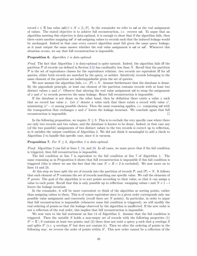
record r ∈ R has value val(r) ∈ X = [1, N ]. In the remainder we refer to val as the real assignmentof values. The stated objective is to achieve full reconstruction, i.e. recover val. To argue that analgorithm meeting this objective is data-optimal, it is enough to show that if the algorithm fails, thenthere exists another mapping val′ 6= val assigning values to records such that the induced leakage wouldbe unchanged. Indeed in that case every correct algorithm must fail given the same query leakage,as it must output the same answer whether the real value assignment is val or val′. Whenever thissituation occurs, we say that full reconstruction is impossible.

Proposition 6. Algorithm 1 is data-optimal.

Proof. The fact that Algorithm 1 is data-optimal is quite natural. Indeed, the algorithm fails iff thepartition P of records (as defined in Section 2.3) has cardinality less than N . Recall that the partitionP is the set of equivalence classes for the equivalence relation: two records are equivalent iff for allqueries, either both records are matched by the query, or neither. Intuitively records belonging to thesame element of the partition are indistinguishable given the set of queries.

We now assume the algorithm fails, i.e. |P| < N . Assume furthermore that the database is dense.By the pigeonhole principle, at least one element of the partition contains records with at least twodistinct values x and x′. Observe that altering the real value assignment val to swap the assignmentof x and x′ to records preserves the same leakage. Hence full reconstruction is impossible.

If the database is not dense on the other hand, then by definition there exists a value x suchthat no record has value x. Let x′ denote a value such that there exists a record with value x′,minimising |x′ − x| among possible choices. Then the same reasoning applies, i.e. composing val withthe transposition that exchanges x and x′ leaves the leakage invariant. We conclude again that fullreconstruction is impossible.

In the following proposition, we require N ≥ 3. This is to exclude the very specific case where thereare only two records and two values, and the database is known to be dense. Indeed, in that case any(of the two possible) assignments of two distinct values to the two records is correct up to reflection,so it satisfies the output condition of Algorithm 2. We did not think it meaningful to add a check toAlgorithm 2 to handle this specific case, since it is vacuous.

Proposition 7. For N ≥ 3, Algorithm 2 is data-optimal.

Proof. Algorithm 2 can fail at lines 7, 14, and 24. In all cases, we must prove that if the fail conditionis triggered, then full reconstruction is impossible.

The fail condition at line 7 is equivalent to the fail condition at line 7 of Algorithm 1. Thesame reasoning as in Proposition 6 shows that full reconstruction is impossible if this fail condition istriggered (this is where we use the fact that the case N = R = 2 is excluded). We now move on tolines 14 and 24.

At this step we have split the set of records into the partition of records P, and |P| = N . It followsthat each element of P contains the set of records matching one specific value. We call the elements ofP points. The goal of the algorithm is to sort points according to their value, so that it can assign avalue to each point. Recall that this is only possible up to reflection: swapping values i and N + 1− ileaves the leakage invariant.

In the remainder, it will be more convenient to think of the algorithm as sorting points, ratherthan assigning values to them. This is of course equivalent since to a given order corresponds only onepossible value assignment and conversely (recall there are N points). In particular, in order to arguethat full reconstruction is impossible (whenever some fail condition is triggered), we will modify thereal ordering of points so that the leakage observed by the algorithm is unaffected. If the new order isnot a reflection of the real order, this implies that full reconstruction is impossible.

We now turn to the fail statement on line 14 of Algorithm 2. Assume that the fail condition istriggered. Then the variable S holds a non-empty set of records with the following properties (1)S′ = R \ S contains at least two points; and (2) there does not exist a query q such that q overlaps Sand splits S′ (i.e. q overlaps S′ but does not contain it). Then we alter the ordering of points in thefollowing way: we reverse the order of points within S′. This new order cannot be a reflection of the

48

original order, since S′ contains at least two points, and their relative ordering is changed; while therelative ordering of points between S and S′ is unaffected.

On the other hand the new order yields the same leakage as the real order: indeed, the only typeof query that could distinguish between these two orders is precisely a query that would split S′ whileoverlapping S. To see this, observe that all other types of queries are either supersets or subsets of S′.The first type contains no information on the ordering of points within S′. The second type cannotbreak the reflection symmetry of elements within S′, for the same reason that we can only solve ouroverall ordering problem up to reflection. Thus full reconstruction is impossible.

The reasoning for the fail condition on line 24 of Algorithm 2 is very similar. If the fail conditionis triggered, we have a set T containing at least two points, such that no query splits T and overlapsT ′ = R \ T . Thus the same reasoning applies. To see that there cannot exist a query q splitting Tand overlapping T ′, first observe that by construction the values of records in I(i) and I(i) ∪ T bothform an initial segment of the set of values (up to reflection). It follows that any query splitting T canoverlap I(i), or R \ (I(i) ∪ T ), but not both. However the first case is impossible due to line 19, andthe second case is ruled out by the loop on line 20.

49