improvement of an aquaculture site-selection model for
TRANSCRIPT

Instructions for use
Title Improvement of an aquaculture site-selection model for Japanese kelp (Saccharina japonica) in southern Hokkaido,Japan : an application for the impacts of climate events
Author(s) Liu, Yang; Saitoh, Sei-Ichi; Radiarta, I. Nyoman; Isada, Tomonori; Hirawake, Toru; Mizuta, Hiroyuki; Yasui, Hajime
Citation ICES Journal of Marine Science, 70(7), 1460-1470https://doi.org/10.1093/icesjms/fst108
Issue Date 2013-11
Doc URL http://hdl.handle.net/2115/57137
RightsThis is a pre-copyedited, author-produced PDF of an article accepted for publication in [ICES journal of marinescience] following peer review. The definitive publisher-authenticated version [ICES J. Mar. Sci. (2013) 70 (7): 1460-1470] is available online at: http://icesjms.oxfordjournals.org/content/early/2013/08/24/icesjms.fst108.
Type article (author version)
File Information final-liu.pdf
Hokkaido University Collection of Scholarly and Academic Papers : HUSCAP
1
Improvement of an aquaculture site-selection model for Japanese kelp (Saccharina 1
japonica) in southern Hokkaido, Japan: An application for the impacts of climate events 2
3
Yang Liu1, Sei-Ichi Saitoh1, I. Nyoman Radiarta2, Tomonori Isada1, Toru Hirawake1, 4
Hiroyuki Mizuta3 and Hajime Yasui4 5
6
1Laboratory of Marine Bioresource and Environment Sensing, Faculty of Fisheries Sciences, 7
Hokkaido University, 3-1-1 Minato, Hakodate, Hokkaido 041-8611, Japan 8 2Research Center for Aquaculture, Agency for Marine and Fisheries Research, Ministry of 9
Marine Affairs and Fisheries. Jl. Ragunan 20, Pasar Minggu, Jakarta 12540, Indonesia 10
3Laboratory of Breeding Science, Faculty of Fisheries Sciences, Hokkaido University, 3-1-1 11
Minato, Hakodate, Hokkaido 041-8611, Japan 12
4Laboratory of Science and Technology on Fisheries Infrastructure System, Faculty of 13
Fisheries Sciences, Hokkaido University, 3-1-1 Minato, Hakodate, Hokkaido 041-8611, Japan 14
15
16
17
*Corresponding author: Yang Liu 18
E-mail: [email protected] , [email protected] 19
Laboratory of Marine Bio resource and Environment Sensing, Faculty of Fisheries Sciences, 20
Hokkaido University, 3-1-1, Minato, Hakodate, Hokkaido, 041-8611, Japan. 21
Tel: +81(138)-40-8844 22
23

2
24
Abstract 25
Japanese kelp (Saccharina japonica) is one of the most valuable cultured and harvested 26
kelp species in Japan. In this study, we added a physical parameter, sea surface nitrate (SSN) 27
estimated from satellite remote sensing data, to develop a suitable aquaculture site-selection 28
model (SASSM) for hanging cultures of Japanese kelp in southern Hokkaido, Japan. The 29
local algorithm to estimate SSN was developed using satellite measurements of sea surface 30
temperature and chlorophyll-a. We found a high correlation between satellite- and 31
ship-measured data (r2 = 0.87, RMSE = 1.39). Multi-criteria evaluation was adapted to the 32
SASSM to rank sites on a scale of 1 (least suitable) to 8 (most suitable). We found that 64.4% 33
of the areas were suitable (score above 7). Minamikayabe was identified as the most suitable 34
area, and Funka Bay also contained potential aquaculture sites. In addition, we examined the 35
impact of El Niño/La Niña–Southern Oscillation (ENSO) events on Japanese kelp aquaculture 36
and site suitability from 2003 to 2010. During El Niño events, the number of suitable areas 37
(scores 7 and 8) decreased significantly, indicating that climatic conditions should be 38
considered for future development of marine aquaculture. 39
40
Keywords: ENSO, Japanese kelp, SASSM, satellite remote sensing, sea surface nitrate. 41
42
43
44
45

3
1. Introduction 46
Approximately 37 species of kelp grow in coastal areas of Japan (Yotsukura, 2010). One of 47
the most important is Japanese kelp (Saccharina japonica, preciously Laminaria japonica). 48
This native kelp is mainly distributed in southern Hokkaido (Ozaki et al., 2001), where it 49
plays a key economic role in coastal communities. Wild harvest has dominated the production 50
of Japanese kelp in Hokkaido (FAO, 2009). However, wild harvest has recently declined from 51
about 30,000 dry tons per year in the 1970s to 14,587 tons in 2009 (Yotsukura, 2010). At the 52
same time, as technology has improved, aquaculture production of Japanese kelp has 53
gradually increased. 54
Because most aquaculture sites are in coastal areas (water depth < 60 m), aquaculture 55
development can be influenced by many factors such as limited suitable areas, multi-use 56
conflicts with other species, environment and climate changes, and impacts of human 57
activities. Understanding the ecology and distribution of foundation species is vital for 58
conservation and coastal management and development (Daniel et al., 2012). Geographic 59
information systems (GIS) and satellite remote sensing technology have been widely used in 60
the development of aquaculture and suitable aquaculture site-selection models (SASSM). 61
Some studies have used SASSM to investigate suitable sites for Japanese kelp aquaculture 62
(Radiarta et al., 2011). However, those models did not consider the nutrient conditions, 63
specifically, nitrate (NO3) conditions. Many studies have indicated that NO3 can be an 64
important factor in the growth and maturation of kelp (e.g., Deysher and Dean, 1986; Mizuta 65
and Maita, 1991; Grant et al., 1998; Gao et al., 2012), but obtaining NO3 data remains 66
difficult. The resolution of NO3 data obtained from conventional shipboard techniques is 67

4
inadequate for regular monitoring over large spatial scales. Satellites are an effective in 68
providing spatial and temporal data. Unfortunately, NO3 cannot be directly measured from 69
space. However, the close relationship of NO3 with sea surface temperature (SST) and 70
chlorophyll-a (Chl-a), which can both be measured using satellite remote sensing, could be 71
utilized to estimate NO3 and extend the resolution of shipboard NO3 estimates (Goes et al., 72
1999). 73
The objectives of this study were to 1) develop local algorithms to estimate sea surface 74
nitrogen (SSN) from remote sensing data in the waters of southern Hokkaido, 2) include the 75
new physical parameter SSN to develop a more accurate SASSM and identify the most 76
suitable areas for Japanese kelp aquaculture, and 3) examine the potential impact of climate 77
change on the development of Japanese kelp aquaculture. 78
79
2. Material and methods 80
Study area 81
The study area was the coastal waters of southern Hokkaido in northern Japan, including 82
Funka Bay and the Tsugaru Strait. This area lies between 41˚40’–42˚10’N and 83
140˚40’–141˚10’E, with mean and maximum depths of 38 m and 107 m, respectively (Fig. 84
1A). The main Japanese kelp aquaculture area is along the coastline from Shikabe to 85
Hakodate, Hokkaido (Fig. 1C). 86
The southern Hokkaido water region, especially Funka Bay, is affected by the coastal 87
Oyashio Current and the Tsugaru Warm Current (TWC) (Ohtani, 1971, 1987; Isoda and 88
Hasegawa, 1997; Takahashi et al., 2005). Warm, saline water occupies Funka Bay from 89

5
October to December, whereas cold, low-salinity water is usually present from March to May. 90
The cold, low salinity water comes from coastal Oyashio water, which sometimes flows into 91
Funka Bay on the southwest coast in winter and spring (Kono et al., 2004). The water in 92
Funka Bay is replaced twice a year, and each replacement takes about 2 months (Miyake et al., 93
1988). These unique characteristics provide favorable environmental conditions for 94
aquaculture activities (Radiarta et al., 2011). On the basis of city administrative boundaries, 95
the aquaculture regions in this water area are divided into six zones. 96
97
Satellite data and processing 98
The data sources used included SST, Chl-a concentration, and suspended solid (SS) 99
concentration, which were derived from the Moderate-Resolution Imaging Spectroradiometer 100
(MODIS) and Sea-Viewing Wide Field-of-View Sensor (SeaWiFS) as level-2 data with 1-km 101
resolution. The 2012.0 MODIS-Aqua reprocessing was completed in May 2012. This study 102
used the new version (R2012.0) of daily data from January 2003 to May 2012. The data were 103
obtained from the Distributed Active Archive Centers (DAAC), Goddard Space Flight Center 104
(GSFC), National Aeronautics and Space Administration (NASA). Monthly averages of nLw 105
(555) images were used to calculate SS images based on Ahn et al.’s (2001) algorithm. 106
Advanced Land Observing Satellite (ALOS) Advanced Visible and Near-Infrared 107
Radiometer type-2 (AVNIR-2) images acquired on 5 Nov. 2009, 5 Oct. 2010, and 7 Dec. 108
2010 with 10-m resolution were downloaded from the ALOS User Interface Gateway (AUIG) 109
website (https://auig.eoc.jaxa.jp/auigs/en/top/index.html) as level 1B2G (geo-coded data). 110

6
These data were used for extracting social-infrastructural and constraint data, such as harbors, 111
town/industrial areas, and river mouths. 112
The bathymetry data were obtained from the Japan Oceanographic Data Center (JODC) 113
and were integrated and gridded at 150-m intervals. 114
To process the remotely sensed data, this study used the SeaWiFS Data Analysis System 115
(SeaDAS) 6.2 and ERDAS imagine 9.3. SeaDAS is a comprehensive image analysis package 116
for processing, displaying, analyzing, and quality controlling ocean color data. The package 117
was developed by GSFC/NASA and is operated in the Linux system. ERDAS Imagine is a 118
remote sensing application with raster graphic editor capabilities that was designed for 119
geospatial applications. The GIS and modeling software used in this study was ArcGIS 10.0, 120
which was developed by the Environmental System Research Institute (ESRI, USA). ERDAS 121
Imagine 9.3 and ArcGIS 10.0 use the Windows XP platform. 122
123
Shipboard data 124
Shipboard data were obtained during 15 cruises on the T/S Oshoro-Maru and R/V 125
Ushio-Maru (Hokkaido University) between April 2010 and January 2012 (Table 1). Optical 126
measurements, conductivity-temperature-depth (CTD) measurements, and water sampling 127
were conducted at 33 stations in Funka Bay and 14 stations in the Tsugaru Strait (Fig. 1B). 128
Water samples for Chl-a were analyzed using a Turner fluorometer. Concentrations of NO3 129
were measured using a QuAAtro segmented flow analyzer and calibrated using reference 130
material from the KANSO Company (http://www.kanso.co.jp/eng/index.html) for nutrients in 131
seawater (RMNS). 132

7
133
Estimating SSN from space 134
Although a very linear relationship may exist between NO3 and seawater temperature (T) 135
based on T–N relationships (Kamykowshi and Zentara, 1986; Chavez and Service, 1996), 136
phytoplankton nitrate uptake also has a significant impact on T–N relationships (Goes et al., 137
2000). Therefore, we used T and Chl-a as the predictor variables to estimate SSN from space. 138
In this study, shipboard data from different cruises were pooled. The data set was restricted to 139
surface water samples. The relationships between NO3 and its predictor variables were 140
examined using the statistical, step-wise linear regression fitting routine of JMP software 141
(SAS Institute). The post-processing of the output SSN data was conducted using 142
image-smoothing technology to remove noise from images. All raster images were smoothed 143
using the Neighborhood Analysis tool (3 3 pixels, mean filter type) of ArcGIS software. 144
145
GIS model construction 146
This study added the physical parameter, SSN, to develop a more accurate SASSM for 147
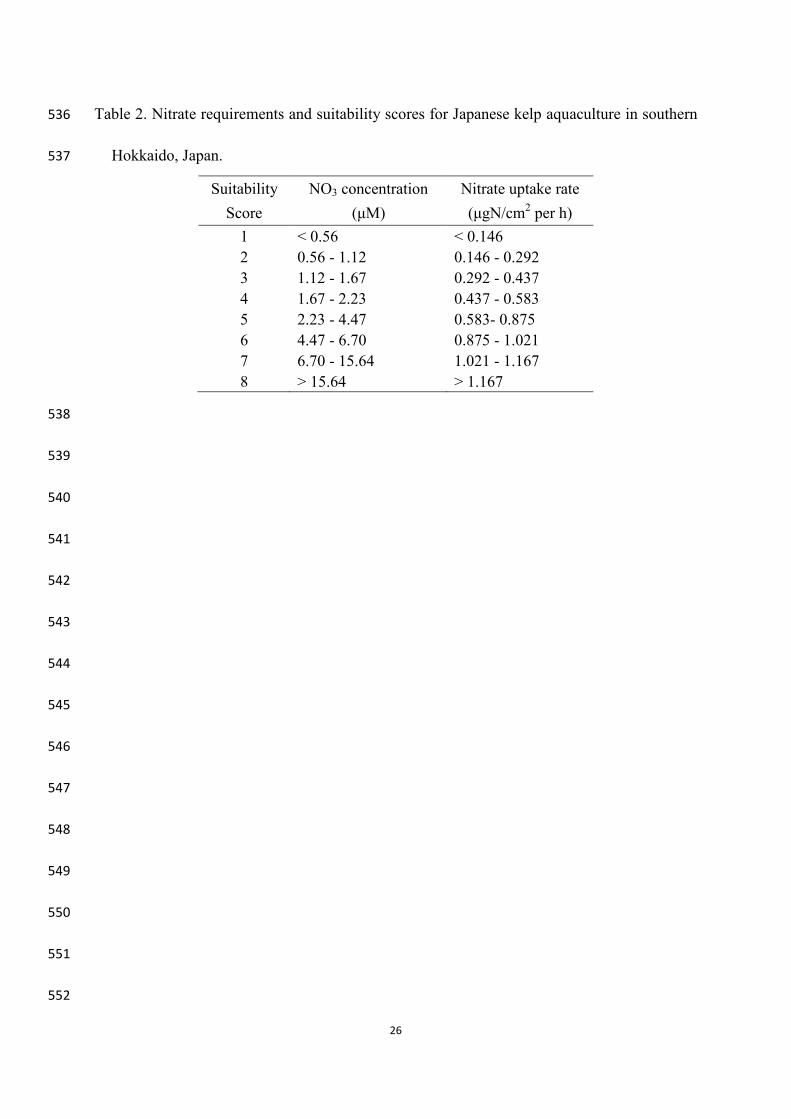
Japanese kelp in southern Hokkaido. Parameter values were ranked and classified into eight 148
levels following Radiarta et al. (2011). Suitable levels (scores) for SSN parameters were 149
defined according to the relationship between nitrate uptakes and nitrate concentrations for 150
discs from Saccharina japonica followed by Michaelis–Menten kinetics (Mizuta, 2003; Ozaki 151
et al., 2001). Nitrate concentrations were determined according to half-saturated concentration 152
(Km) (Parsons et al., 1984) and the maximum uptake rate (Vmax) (Wilkinson, 1961). Based on 153
Ozaki et al.’s (2001) results, Km = 1.7 μM, Vmax = 1.2 μgN/cm2/h and Km = 3.3 μM, Vmax = 154

8
1.0 μgN/cm2/h for the median and marginal parts of Saccharina japonica, respectively, were 155
used in this study. The area ratio of the median and marginal parts of the spores of Saccharina 156
japonica was 1:2; therefore, the final results of Km = 2.23 μM and Vmax = 1.17μgN/cm2/h 157
were obtained by averaging each part and multiplying by the area ratio. NO3 concentrations 158
were ranked and classified from 1 (least suitable) to 8 (most suitable) by calculations from 159
nitrate uptake rates at 0.146 μgN/cm2/h (Table 2). 160
Figure 2 shows the schematic framework for the Japanese kelp SASSM. The GIS model 161
was formed by three sub-models including the biophysical model (SST, SS, SSN, bathymetry, 162
and slope), social-infrastructural model (distance to a town or city, pier and land-based 163
facilities), and constraints model (harbor, area near town, and river mouth). Parameter weights 164
were determined by pairwise comparisons according to the analytical hierarchy process for 165
decision making (Saaty, 1977). The kelp productions of each zone were used to verify the 166
model. Finally, to model the potential impact of climate variation on kelp aquaculture, we 167
analyzed years with different climatology (El Niño and normal years) during 2003 to 2010. 168
169
3. Results 170
Local algorithm for SSN development 171
Some studies have estimated SSN in the Pacific using satellite-observed data (Goes et al., 172
1999; Switzer et al., 2003). However, few studies have focused on the regional scale, 173
especially Funka Bay, Japan. We developed local algorithms to examine variations in SSN as 174
a function of SST and Chl-a in the waters of southern Hokkaido. Before the calculations, we 175
verified the accuracy of the predictors from the satellite remote sensing data. Comparison of 176
9
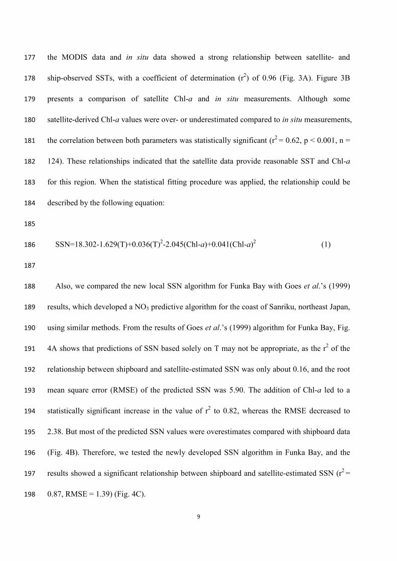
the MODIS data and in situ data showed a strong relationship between satellite- and 177
ship-observed SSTs, with a coefficient of determination (r2) of 0.96 (Fig. 3A). Figure 3B 178
presents a comparison of satellite Chl-a and in situ measurements. Although some 179
satellite-derived Chl-a values were over- or underestimated compared to in situ measurements, 180
the correlation between both parameters was statistically significant (r2 = 0.62, p < 0.001, n = 181
124). These relationships indicated that the satellite data provide reasonable SST and Chl-a 182
for this region. When the statistical fitting procedure was applied, the relationship could be 183
described by the following equation: 184
185
SSN=18.302-1.629(T)+0.036(T)2-2.045(Chl-a)+0.041(Chl-a)2 (1) 186
187
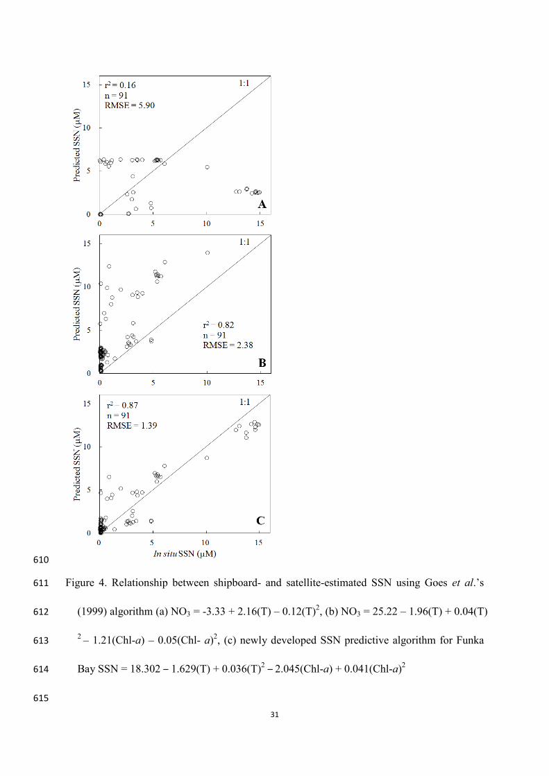
Also, we compared the new local SSN algorithm for Funka Bay with Goes et al.’s (1999) 188
results, which developed a NO3 predictive algorithm for the coast of Sanriku, northeast Japan, 189
using similar methods. From the results of Goes et al.’s (1999) algorithm for Funka Bay, Fig. 190
4A shows that predictions of SSN based solely on T may not be appropriate, as the r2 of the 191
relationship between shipboard and satellite-estimated SSN was only about 0.16, and the root 192
mean square error (RMSE) of the predicted SSN was 5.90. The addition of Chl-a led to a 193
statistically significant increase in the value of r2 to 0.82, whereas the RMSE decreased to 194
2.38. But most of the predicted SSN values were overestimates compared with shipboard data 195
(Fig. 4B). Therefore, we tested the newly developed SSN algorithm in Funka Bay, and the 196
results showed a significant relationship between shipboard and satellite-estimated SSN (r2 = 197
0.87, RMSE = 1.39) (Fig. 4C). 198

10
199
Verification and seasonal variability in the predicted SSN 200
Using the developed local algorithm, we generated 113 predicted monthly SSN maps (from 201
January 2003 to May 2012). To reflect the spatial distribution of predicted SSN 202
concentrations in the coastal waters of southern Hokkaido, the monthly maps for 2010 were 203
used as an example (Fig. 5). The predicted SSN concentration began to increase in December 204
and reached its maximum in February (12–15 μM), but was very low from April to October. 205
In particular, predicted concentrations were less than 1μM during August and September. 206
This finding is consistent with other local studies (Maita et al., 1991; Kudo et al., 2000), and 207
it occurs because of the nutrient-rich period in the photic zone supplied by strong vertical 208
mixing during winter (Sugie et al., 2010). 209
Some satellite data were affected by clouds on the observation dates and could not be used. 210
Therefore, we compared the shipboard SSN for stations ST.13 and SE.9 (see Fig. 1B) during 211
April 2010 to January 2012 and satellite-estimated SSN on clear observation days during 212
January 2003 to May 2012 to verify the accuracy of the predicted values and show seasonal 213
variability. The results are shown in Fig. 6. The seasonal variation in SSN had higher values 214
in the winter (average 14.8 μM in February) and lower values in the summer (average 0.07 215
μM in August). The predicted SSN was consistent with the in situ data. The SSN suddenly 216
deceased from March-April, which may have been a result of the occurrence of a spring 217
bloom. The concentration of Chl-a increased significantly in March (Maita et al., 1991; 218
Sasaki et al., 2005). Phytoplankton biomass was found to be limited by NO3, and the 219

11
exhaustion of NO3 was observed in the photic zone at the end of the bloom (Levasseur and 220
Therriault, 1987; Kudo et al., 2000). 221
222
Model of the spatial distribution of suitability 223
On the basis of a previous model (Radiarta et al., 2011), the improved SASSM was 224
developed. Using 2010 data as an example, we compared the previous model (Fig. 7A) with 225
the new models. The improvement included two steps, with the first being improved 226
bathymetry. Comparison of the new distribution map (Fig. 7B) with the previous map shows 227
slight differences in the potential area at Shikabe and Minamikayabe. This was a result of the 228
previous model using 500-m gridded bathymetric data, whereas the new model (Fig. 7B) used 229
more accurate 150-m gridded bathymetric data. However this did not result in any change in 230
suitable areas. The second step involved adding an SSN parameter to improve the model. The 231
new model (Fig. 7C) shows that the difference is in the distribution of the suitable area, 232
especially areas with the highest suitability score of 8 (dark blue color). The previous (Fig. 7A) 233
study showed that the most suitable areas (score 8) were distributed along the coast from 234
Oshamanbe to Yakumo in Funka Bay, and also in the Shikabe, Minamikayabe, Todohokke, 235
Esan, and Toi areas. According to the field survey and kelp production statistics from the 236
Hokkaido government (Marinenet Hokkaido, 2010), the main kelp culture area is along the 237
coastline from Shikabe to Hakodate, with the highest production in the Minamikayabe area. 238
In other places, there was no kelp production inside Funka Bay; therefore, the relationship 239
between high scores by the previous model and in situ kelp production has some 240
contradictions. However, when the new physical parameter of SSN was included, the most 241

12
suitable area was still shown in the main kelp culture areas but was no longer shown in Funka 242
Bay. The new model (Fig. 7C) was well verified by in situ kelp production. 243
244
Temporal variations in suitability area 245
The final models of the growing season (May–July) for Japanese kelp aquaculture in 246
southern Hokkaido during 2003 to 2010 are shown in Fig. 8. These results showed high 247
suitability scores (above 7) for most of the kelp aquaculture areas in southern Hokkaido 248
during the growing season, especially Minamikayabe, which was the most suitable area (score 249
8). The waters near Hakodate Mountain were less suitable (score 5) for kelp aquaculture. 250
From the comparison of suitable areas during the 8 years, it was observed that the most 251
suitable areas (scores 7 and 8) decreased significantly in 2004, 2007, and 2010. 252
253
Climate events and Kelp production 254
The sustainability of aquaculture can be influenced by environmental changes (Taylor et al., 255
2008; Cocharane et al., 2009; Baba et al., 2009; Saitoh et al., 2011). However, few studies 256
have explored the impacts of climate change on Japanese kelp aquaculture. Therefore, we 257
combined suitability scores with kelp production and climatic events, namely the El Niño/La 258
Niña–Southern Oscillation (ENSO), to examine the potential impacts of climate change on the 259
development of Japanese kelp aquaculture. The Oceanic Niño Index (ONI) was used as a 260
measure of the strength of an ENSO episode 261
(http://gcmd.nasa.gov/records/GCMD_NOAA_NWS_CPC_ONI.html). We sorted El Niño 262
and La Niña episodes into three categories, strong, moderate, and weak, based on ONI values. 263

13
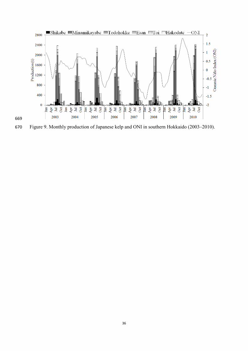
The thresholds for ONI values were obtained from Chris and Stan (2008). From the monthly 264
time series of ONI during 2003–2012 (Fig. 9), El Niño was found to occur during 2004–2005, 265
2006–2007, and 2009–2010, and La Niña occurred during 2008–2009 and 2010–2011. 266
Monthly kelp production data (Fig. 9) are published by the Fisheries Department of the 267
Hokkaido government and are available at the Marinenet Hokkaido website: 268
http://www.fishexp.hro.or.jp/marineinfo/internetdb/index.htm. The annual kelp production of 269
Minamikayabe accounts for about 60% of total Hokkaido kelp production. Production has 270
changed over the years, especially decreasing in 2004 and 2007. 271
272
4. Discussion 273
Estimated SSN and improved SASSM model 274
Previous studies that have examined site-selection models have focused on the physical 275
parameters of SST, SS, bathymetry, and slope. However, the present study demonstrates that 276
the model could be improved by including local southern Hokkaido water characteristics. 277
Because NO3 is an essential element for Japanese kelp growth, this study considered the SSN 278
to develop a more accurate model. Many studies have demonstrated the possibility of 279
estimating SSN at a large scale based on satellite SST because of the sensitivity of T–N 280
relationships (Traganza et al., 1983; Switzer et al., 2003). Also, phytoplankton nitrate uptake 281
could have a significant impact on T–N relationships (Goes et al., 2000). Therefore, we 282
developed a local algorithm to estimate SSN based on T and Chl-a in southern Hokkaido. In 283
comparing this algorithm with other NO3 predictive algorithms (see Fig. 4), we understand 284
that different water regions have different dynamics. If this approach were to be applied in 285

14
other regions, we recommend a starting point of shipboard nitrate measurements for the 286
development of a new, location-specific algorithm. Additionally, satellite-predicted SSNs are 287
not as accurate as shipboard measurements, and SSN concentrations along coastal regions are 288
highly susceptible to the effects of human activities, such as agricultural sewage discharge 289
(Del Amo et al., 1997). Therefore, satellite data cannot replace shipboard measurements, but 290
can be a useful tool for obtaining synoptic information on SSN concentrations. With advances 291
in satellite technology, satellite-based estimates will continue to improve. 292
The final results of the improved SASSM showed increased accuracy in the actual kelp 293
culture region, which was verified by kelp production statistics for Hokkaido. However, 294
regions that have not been producing kelp may also be suitable for aquaculture. The 295
suitability map (Fig. 7C) showed a score of 7 along most of the coastline. Field surveys 296
indicated that certain amounts of wild kelp exist in Funka Bay, although few commercial kelp 297
enterprises are found in this area. This may be because aquaculture production in Funka Bay 298
focuses mainly on cultured scallop. To avoid multi-use conflicts within the limited 299
aquaculture area, few kelp cultures are found in Funka Bay. However, Japanese kelp is an 300
important traditional product in southern Hokkaido. In Minamikayabe, more than 2000 301
fishermen engage in kelp aquaculture, which has increased the kelp production in this area. 302
Therefore, with reasonable planning and management, Funka Bay may be a potential area for 303
Japanese kelp culture. 304
305
Relationships among ENSO, currents, and kelp aquaculture zones 306

15
The Oyashio is a western boundary current of subarctic circulation in the North Pacific. In 307
recent years the southward intrusion of the Oyashio has shown large seasonal variation and 308
comparable interannual variations (Qiu, 2002), and it has been observed that these variations 309
are associated with global changes in atmospheric circulation (Sekine, 1988; Tatebe and 310
Yasuda, 2005). The dominant climate variabilities in the western North Pacific are high 311
frequency variations associated with ENSO events (McKinnell and Dagg, 2010). 312
Conversely, the Tsushima Warm Current is the only major warm current flowing in the 313
Japan Sea, and it forms a major part of the volume transport of the TWC, which flows into the 314
North Pacific Ocean through the Tsugaru Strait (Ohtani, 1987; Onishi and Ohtani, 1997). 315
Seasonal variations in flow corresponded to seasonal changes in the sea level differences 316
between the Japan Sea side and Pacific Ocean side of the Tsugaru Strait (Nishida et al., 2003; 317
Tanno et al., 2005). Hirose and Fukudome (2006) showed a relationship between the volume 318
transport of the TWC in autumn and interannual variation in local evaporation and 319
precipitation in winter. Also, Yasuda and Hanawa (1997) suggested that variation in the TWC, 320
as part of the western boundary current of the subtropical gyre, is influenced by atmospheric 321
and oceanic variability over the North Pacific. ENSO events have been implicated as major 322
factors controlling the winter climate over the North Pacific (Zhang et al., 1996). Lyu and 323
Kim (2003) suggested that long-term variations in transport through the Tsushima Strait are 324
related to changes, such as El Niño, in the Pacific Ocean. Hong et al.’s (2001) results showed 325
that variation in the SST anomaly in the Japan Sea occurs simultaneously with the 326
development of ENSO events in the tropical Pacific Ocean. Additionally, Hirose et al.’s 327

16
(2009) results indicated that the western Pacific index in winter follows the volume transport 328
of the TWC in autumn and connects with the El Niño index. 329
Therefore, the oceanic variability and atmospheric circulation are strongly coupled. Climate 330
change associated spatial and temporal fluctuations in the Coastal Oyashio Current and TWC 331
can have significant influences on Japanese kelp aquaculture along the coast of southern 332
Hokkaido. The mature phase of an ENSO often occurs in winter, and the growing season of 333
Japanese kelp is from May to July. Therefore, we attempted to compare suitable areas and 334
kelp production in El Niño years with those in other years to determine the impacts of a 335
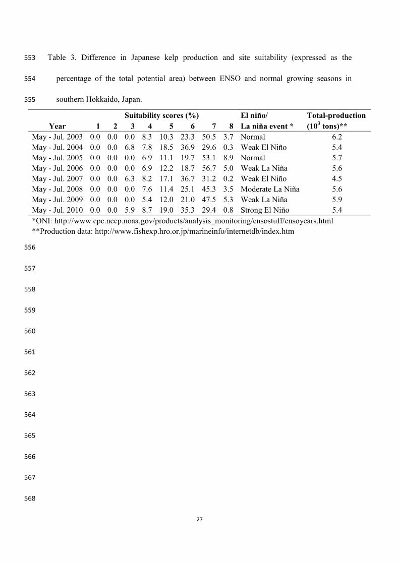
climate event (El Niño event) on the growing season of Japanese kelp aquaculture. Table 3 336
shows differences in Japanese kelp production and site suitability with ENSO events during 337
2003 to 2010. The suitability scores of sites in an El Niño year differed from those in a 338
normal year. During El Niño, the suitable sites (scores 7 and 8) decreased significantly 339
compared with other years. The amount of suitable area (score 8) decreased by 0.3%, 0.2%, 340
and 0.8% in 2004, 2007, and 2010, respectively. In other years, more than 3.5% of the area 341
was rated as the most suitable. These results are consistent with actual kelp production data, 342
which showed total production of 5.4, 4.5, and 5.4 thousand tons in 2004, 2007, and 2010, 343
respectively. Such changes may reflect the impact of climate change through seawater 344
temperature on aquaculture areas. Japanese kelp is a temperate cold water species, and when 345
seawater temperatures exceed 23°C, most of the kelp blade will rot (FAO, 346
http://www.fao.org/fishery/culturedspecies/Laminaria_japonica/en). The harvest season is 347
from July to September (see Fig. 9). During El Niño events, the seawater temperature 348
increases in this region, which can shorten the kelp growing season and reduce production. 349
17
Thus, during El Niño years, kelp harvesters should closely monitor changes in water 350
temperatures and prepare to harvest earlier than in a normal year. 351
352
5. Conclusion 353
This study proposes a method to estimate SSN at a local scale using satellite-observed SST 354
and chlorophyll-a. The improved SASSM effectively identified the most suitable areas for 355
Japanese kelp aquaculture in southern Hokkaido, and the results were consistent with in situ 356
production data. In addition to the traditional Japanese kelp aquaculture area, we also 357
identified some potentially suitable aquaculture areas in Funka Bay, which can provide a basis 358
for future management. We also examined the impacts of climate change on the availability of 359
suitable sites. The results suggested that climate variability could influence the development 360
of Japanese kelp aquaculture through changes in site suitability. These changes should be 361
considered when managing kelp aquaculture. 362
363
Acknowledgements 364
This work was supported by “Hakodate Marine Bio Cluster Project” in the knowledge 365
Cluster Program from 2009 and the Grant-in-Aid for the Regional Innovation Strategy 366
Support Program (Global Type) from the Ministry of Education, Culture, Sports, Science and 367
Technology (MEXT), Japan. It was also supported by the Japan Aerospace Exploration 368
Agency (JAXA) SGLI/GCOM-C Project. Especially, we appreciate two anonymous 369
reviewers for providing constructive comments. 370
371
18
References 372
Ahn, Y.H., Moon, J.E., and Gallegos, S. 2001. Development of suspended particulate matter 373
algorithms for ocean color remote sensing. Korean Journal of Remote Sensing, 17: 374
285-295. 375
Baba, K., Sugawara, R., Nitta, H., Endou, K., and Miyazono, A. 2009. Relationship between 376
spat density, food availability, and growth of spawners in cultured Mizuhopecten 377
yessoensis in Funka Bay: concurrence with El Niño Sounthern Oscillation. Canadian 378
Journal of Fisheries and Aquatic Sciences, 66: 6-17. 379
Chavez, F.P., and Service, S.K.1996. Temperature-nitrate relationships in the central and 380
eastern tropical Pacific. Journal of Geophysical Research, 101: 20553-20563. 381
Chris, S., and Stan, C. 2008. El Niño and La Niña episodes and their impact on the weather in 382
the Las Vegas Valley, National Weather Service, Las Vegas, NV. Available online: 383
http://www.wrh.noaa.gov/vef/projects.php. 384
Cocharane, K., Young, C.D., Soto, D., and Bahri, T. 2009. Climate change implications for 385
fisheries and aquaculture: overview of current scientific knowledge. FAO Fisheries and 386
aquaculture technical paper No. 530. UNEP. 2009. The climate change fact sheet. 387
Daniel, G., Touria, B., Jacques, P., Mickaël, V., and Axel, E. 2012. Modeling kelp forest 388
distribution and biomass along temperate rocky coastlines. Marine Biology, Doi: 389
10.1007/s00227-012-2089-0. 390
Del Amo, Y., Le Pape, O., Tréguer, P., Quéguiner, B., Ménesguen, A., and Aminot, A. 1997. 391
Impacts of high-nitrate freshwater inputs on macrotidal ecosystems. I. Seasonal evolution 392

19
of nutrient limitation for the diatom-dominated phytoplankton of the Bay of Brest (France). 393
Marine Ecology Progress Series, 161: 213-224. 394
Deysher, L.E., and Dean, T.A. 1986. In situ recruitment of sporophytes of the giant kelp, 395
Macrocystis pyrifera (L.) C.A. Agardh: effects of physical factors. Journal of Experimental 396
Marine Biology and Ecology, 103: 41-63. 397
FAO 2004-2013. Cultured Aquatic Species Information Programme. Laminaria japonica. 398
Cultured Aquatic Species Information Programme. Text by Chen, J. In: FAO Fisheries and 399
Aquaculture Department. Rome. Updated 1 January 2004. 400
http://www.fao.org/fishery/culturedspecies/Laminaria_japonica/en (last accessed 21 June 401
2013). 402
FAO website. FAO Fisheries and Aquaculture Department: Laminaria japonica. 403
http://www.fao.org/fishery/culturedspecies/Laminaria_japonica/en. 404
Gao, X., Agatsuma, Y., and Taniguchi, K. 2012. Effect of nitrate fertilization of gametophytes 405
of the kelp Undaria pinnatifida on growth and maturation of the sporophytes cultivated in 406
Matsushima Bay, northern Honshu, Japan. Aquaculture International, Doi: 407
10.1007/s10499-012-9533-5. 408
Goes, J.I., Saino, T., Oaku, H., and Jiang, D.L. 1999. A method for estimating sea surface 409
nitrate concentrations from remotely sensed SST and Chlorophyll a – A case study for the 410
North Pacific Ocean using OCTS/ADEOS data. IEEE Transactions on Geoscience and 411
Remote Sensing, 37: 1633-1644. 412

20
Goes, J.I., Saino, T., Oaku, H., Ishizaka, J., Wong, C.S., and Nojiri, Y. 2000. Basin scale 413
estimates of Sea Surface Nitrate and New Production from remotely sensed Sea Surface 414
Temperature and Chlorophyll. Geophysical Research Letters, 27: 1263-1266. 415
Grant, J., Stenton-Dozey, J., Montiero, P., Pitcher, G., and Heasman, K. 1998. Shellfish 416
culture in the Benguela system: A carbon budget of Saldanha Bay for raft culture of 417
Mytilus Galloprovincialis. Journal of Shellfish Research, 17: 41-49. 418
Hirose, N., and Fukudome, K. 2006. Monitoring the Tsushima Warm Current improves 419
seasonal prediction of the regional snowfall, Scientific Online Letters on the Atmosphere, 2: 420
61-63. 421
Hirose, N., Nishimura, K., and Yamamoto, M. 2009. Observational evidence of a warm ocean 422
current preceding a winter teleconnection pattern in the northwestern Pacific. Geophysical 423
Research Letters, 36, L09705, doi:10.1029/2009GL037448. 424
Hong, C.H., Cho, K.D., and Kim, H.J. 2001. The relationship between ENSO events and sea 425
surface temperature in the East Japan Sea. Progress in Oceanography, 49: 21-40. 426
Isoda, Y., and Hasegawa, K. 1997. Heat budget of Funka Bay. Umi to Sora, 3: 93-101. (in 427
Japanese) 428
Kamykowski, D., and Zentara, S.J. 1986. Predicting plant nutrient concentrations from 429
temperature and sigma-t in the upper kilometer of the world ocean. Deep Sea Research, 33: 430
89-105. 431
Kono, T., Foreman, M., Chandler, P., and Kashiwai, M. 2004. Coastal Oyashio south of 432
Hokkaido, Japan. Journal of Physical Oceanography, 34: 1477-1494. 433

21
Kudo, I., Yoshimura, Y., Yanada, M., and Matsunaga, K. 2000. Exhaustion of nitrate 434
terminates a phytoplankton bloom in Funka Bay, Japan: change in SiO4:NO3 consumption 435
rate during the bloom. Marine Ecology Progress Series, 193: 45-51. 436
Levasseur, M.E., and Therriault, J.C. 1987. Phytoplankton biomass and nutrient dynamics in a 437
tidally induced upwelling: the role of the NO3:SiO4 ratio. Marine Ecology Progress Series, 438
39: 87-97. 439
Lyu, S.J., and Kim, K. 2003. Absolute transport from the sea level difference across the Korea 440
Strait. Geophysical research letters, 30: 1285, doi:10.1029/2002GL016233. 441
Maita, Y., Mizuta, H., and Yanada, M. 1991. Nutrient environment in natural and cultivated 442
grounds of Laminaria japonica. Bulletin of the Faculty of Fisheries Hokkaido University, 443
42: 98-106. 444
Marinenet Hokkaido. 2010. Search and aggregate statistics of the fishery catch from 1991 to 445
2010. http://www.fishexp.hro.or.jp/marineinfo/internetdb/index.htm. 446
McKinnell, S.M., and Dagg, M.J. 2010. Marine ecosystems of the North Pacific ocean, 447
2003-2008. PICES Special Publication, 4, 393p. 448
Miyake, H., Tanaka, I., and Murakami, T. 1988. Outflow of water from Funka Bay, Hokkaido, 449
during early spring. Journal of the Oceanographical Society of Japan, 44: 163-170. 450
Mizuta, H. 2003. Distribution of Laminaria Species in the Coastal Oyashio Region and their 451
Nutrient Requirements. Bulletin on Coastal Oceanography, 41: 33-38. (in Japanese) 452
Mizuta, H., and Maita, Y. 1991. Effects of nitrate supply on ammonium assimilations in the 453
blade of Laminaria japonica (Phaeophyceae). Bulletin of the faculty of fisheries Hokkaido 454
University, 42: 107-114. 455
22
Nishida, Y., Kanomata, I., Tanaka, I., Sato, S., Takahashi, S., and Matsubara, H. 2003. 456
Seasonal and Interannual Variations of the Volume Transport through the Tsugaru Strait. 457
Oceanography in Japan, 12: 487-499. (in Japanese) 458
Ohtani, K. 1971. Studies on the change of the hydrographic conditions in the Funka BayⅡ. 459
Characteristics of the water occupying the Funka Bay. Bulletin of the faculty of fisheries 460
Hokkaido University, 22: 58-66. 461
Ohtani, K. 1987. Westward Inflow of the Coastal Oyashio Water into the Tsugaru Strait. 462
Bulletin of the Faculty of Fisheries, Hokkaido University, 38: 209-220. (in Japanese) 463
Onishi, M., and Ohtani, K. 1997. Volume transport of the Tsushima Warm Current, west of 464
Tsugaru Strait bifurcation area. Journal of Oceanography, 53: 27-34. 465
Ozaki, A., Mizuta, H., and Yamamoto, H. 2001. Physiological differences between the 466
nutrient uptakes of Kjellmaniella crassifolia and Laminaria japonica (Phaeophyceae). 467
Fisheries Science, 67: 415-419. 468
Parsons, T.R., Maita, Y., and Lalli, C.M. 1984. A manual for chemical and biological 469
methods for seawater analysis. Pergamon Press, New York. 470
Qiu, B. 2002. Large-scale variability in the midlatitude subtropical and subpolar North Pacific 471
Ocean: Observations and causes. Journal of Physical Oceanography, 32: 353-375. 472
Radiarta, I N., Saitoh, S-I., and Yasui, H. 2011. Aquaculture site selection for Japanese kelp 473
(Laminaria japonica) in southern Hokkaido, Japan, using satellite remote sensing and 474
GIS-based models. ICES Journal of Marine Science, 68: 773-780. 475
Saaty, T.L. 1977. A scaling method for priorities in hierarchical structures. Journal of 476
Mathematical Psychology, 15: 234-281. 477

23
Saitoh, S-I., Mugo, R., Radiarta, I N., Asaga, S., Takahashi, F., Hirawake, T., Ishikawa, Y., 478
Awaji, T., In, T., and Shima, S. 2011. Some operational uses of satellite remote sensing 479
and marine GIS for sustainable fisheries and aquaculture. ICES Journal of Marine Science, 480
68: 687-695. 481
Sasaki, H., Miyamura, T., Saitoh, S-I., and Ishizaka, J. 2005. Seasonal variation of absorption 482
by particles and colored dissolved organic matter (CDOM) in Funka Bay, southwestern 483
Hokkaido, Japan. Estuarine, Coastal and Shelf Science, 64: 447-458. 484
Sekine, Y. 1988. Anomalous southward intrusion of the Oyashio east of Japan: 1. Influence of 485
the seasonal and interannual variations in the wind stress over the North Pacific, Journal of 486
Geophysical Research, 93: 2247–2255. 487
Sugie, K., Kuma, K., Fujita, S., Nakayama, Y., and Ikeda, T., 2010. Nutrient and diatom 488
dynamics during late winter and spring in the Oyashio region of the western subarctic 489
Pacific Ocean. Deep-Sea Research Ⅱ, 57: 1630-1642. 490
Switzer, A.C., Kamykowski, D., and Zentara, S.J. 2003. Mapping nitrate in the global ocean 491
using remotely sensed sea surface temperature. Journal of Geophysical Research, 108, 492
doi:10.1029/2000JC000444. 493
Takahashi, D., Nishida, Y., Kido, K., Nishina, K., and Miyake, H. 2005. Formation of the 494
summertime anticyclonic eddy in Funka Bay, Hokkaido Japan. Continental Shelf Research, 495
25: 1877-1893. 496
Tanno, T., Kuroda, H., Isoda, Y., and Aiki, T. 2005. Flow variations off Cape of Esan, 497
northeast of Tsugaru Strait. Bulletin of Fisheries Sciences, Hokkaido University, 56: 33-41. 498
(in Japanese) 499

24
Tatebe, H., Yasuda, I. 2005. Interdecadal variations of the coastal Oyashio from the 1970s to 500
the early 1990s. Geophysical Research Letters, 32: L10613, doi:10.1029/2005GL022605. 501
Toylor, M.H., Wolff, M., Mendo, J., and Yamashiro, G. 2008. Changes in trophic flow 502
structure of independence Bay (Peru) over an ENSO cycle. Progress in Oceanography, 79: 503
336-351. 504
Traganza, E.D., Silva, V.M., Austin, D.M., Hanson, W.L., and Bronsink, S.H. 1983. Nutrient 505
mapping and recurrence of coastal upwelling centers by satellite remote sensing: Its 506
implication to primary production and the sediment record. In E.Suess, and J. Thiede (Eds.), 507
Coastal upwelling. Its sediment record. Part A (pp.61-83). Plenum. 508
Wilkinson, G.N. 1961. Statistical estimations in enzyme kinetics. Biochemical Journal, 80: 509
824-832. 510
Yasuda, T., and Hanawa, K. 1997. Decadal changes in the mode waters in the midlatitude 511
North Pacific. Journal of Physical Oceanography, 27: 858-870. 512
Yotsukura, N. 2010. Production of kelp in Japan: various natural resources and the established 513
aquaculture technique. Seaweeds for human consumption, Bioactive Compounds, and 514
Combating of Diseases: An international interdisciplinary symposium, Carlsberg Academy, 515
Copenhagen, August 26-27, 2010. 516
Zhang, R., Sumi, A., and Kimoto, M. 1996. Impact of El Niño on the East Asian monsoon: A 517
diagnostic study of the ’86/87 and ’91/92 events. Journal of the Meteorological Society of 518
Japan, 74: 49-62. 519
520
521

25
Table 1. Water sampling during the cruises (Apr. 2010 – Jan. 2012) on the T/S Oshoro-Maru 522
and R/V Ushio-Maru in southern Hokkaido, Japan. 523
Year Date Cruise Number of Stations
2010 Apr.19-21 US194 32 May 21-23 US196 11 Jun.19 US199 16 Aug.20-22 US201_1 23 Aug.28-30 US201_2 15 Oct.21-23 US208 32 Nov.10-13 US210 15
2011 Feb.6-8 US219 11 Feb.24 OS225 12
Mar.6 US222 1 May14-16 US228 23 Jul.27-28 US232 13 Sep.27-29 US237 10 Nov.17-19 US242 10
2012 Jan.10 US246 5
524
525
526
527
528
529
530
531
532
533
534
535
26
Table 2. Nitrate requirements and suitability scores for Japanese kelp aquaculture in southern 536
Hokkaido, Japan. 537
Suitability NO3 concentration Nitrate uptake rate Score (μM) (μgN/cm2 per h)
1 < 0.56 < 0.146 2 0.56 - 1.12 0.146 - 0.292 3 1.12 - 1.67 0.292 - 0.437 4 1.67 - 2.23 0.437 - 0.583 5 2.23 - 4.47 0.583- 0.875 6 4.47 - 6.70 0.875 - 1.021 7 6.70 - 15.64 1.021 - 1.167 8 > 15.64 > 1.167
538
539
540
541
542
543
544
545
546
547
548
549
550
551
552
27
Table 3. Difference in Japanese kelp production and site suitability (expressed as the 553
percentage of the total potential area) between ENSO and normal growing seasons in 554
southern Hokkaido, Japan. 555
Year Suitability scores (%) El niño/ Total-production
1 2 3 4 5 6 7 8 La niña event * (103 tons)** May - Jul. 2003 0.0 0.0 0.0 8.3 10.3 23.3 50.5 3.7 Normal 6.2 May - Jul. 2004 0.0 0.0 6.8 7.8 18.5 36.9 29.6 0.3 Weak El Niño 5.4 May - Jul. 2005 0.0 0.0 0.0 6.9 11.1 19.7 53.1 8.9 Normal 5.7 May - Jul. 2006 0.0 0.0 0.0 6.9 12.2 18.7 56.7 5.0 Weak La Niña 5.6 May - Jul. 2007 0.0 0.0 6.3 8.2 17.1 36.7 31.2 0.2 Weak El Niño 4.5 May - Jul. 2008 0.0 0.0 0.0 7.6 11.4 25.1 45.3 3.5 Moderate La Niña 5.6 May - Jul. 2009 0.0 0.0 0.0 5.4 12.0 21.0 47.5 5.3 Weak La Niña 5.9 May - Jul. 2010 0.0 0.0 5.9 8.7 19.0 35.3 29.4 0.8 Strong El Niño 5.4 *ONI: http://www.cpc.ncep.noaa.gov/products/analysis_monitoring/ensostuff/ensoyears.html **Production data: http://www.fishexp.hro.or.jp/marineinfo/internetdb/index.htm
556
557
558
559
560
561
562
563
564
565
566
567
568

28
Figure captions 569
570
Figure 1. (a) Study area in southern Hokkaido, Japan. (b) Filled circles represent local 571
sampling stations in Funka Bay and the Tsugaru Strait. The star marked D is ST.13, and the 572
star marked E is SE.9. (c) Zones of marine aquaculture in southern Hokkaido, Japan. 573
574
575
576
577
578
579
580
581

29
582
Figure 2. Hierarchical scheme and parameter weights of the SASSM for Japanese kelp in 583
southern Hokkaido, Japan. 584
585
586
587
588
589
590
591
592

30
593
Figure 3. Variation in (a) SST and (b) Chl-a between in situ and satellite data in southern 594
Hokkaido, Japan. 595
596
597
598
599
600
601
602
603
604
605
606
607
608
609
31
610
Figure 4. Relationship between shipboard- and satellite-estimated SSN using Goes et al.’s 611
(1999) algorithm (a) NO3 = -3.33 + 2.16(T) – 0.12(T)2, (b) NO3 = 25.22 – 1.96(T) + 0.04(T) 612
2 – 1.21(Chl-a) – 0.05(Chl- a)2, (c) newly developed SSN predictive algorithm for Funka 613
Bay SSN = 18.302 – 1.629(T) + 0.036(T)2 – 2.045(Chl-a) + 0.041(Chl-a)2 614
615

32
616
Figure 5. Monthly images of predicted SSN (μM) during Jan. 2010 to Dec. 2010 in the waters 617
of Southern Hokkaido, Japan. 618
619
620

33
621
Figure 6. Seasonal variability and variation in in situ and satellite-predicted SSN (μM) at 622
stations ST.13 and SE.9 during Jan. 2003 to May 2012 in southern Hokkaido, Japan. 623
624
625
626
627
628
629
630
631
632
633
634
635
636
637

34
638
Figure 7. Suitability sites maps for Japanese kelp aquaculture in 2010 using (a) the previous 639
model, (b) the SASSM with improved bathymetry, (c) the SASSM with improved 640
bathymetry and SSN. 641
642
643
644
645
646
647
648
649
650
651
652
653
654

35
655
Figure 8. SASSM maps for Japanese kelp during the growing season (May–July) in southern 656
Hokkaido, 2003 to 2010. 657
658
659
660
661
662
663
664
665
666
667
668
36
669
Figure 9. Monthly production of Japanese kelp and ONI in southern Hokkaido (2003–2010). 670