improvement of resonant harmonic filter effectiveness in
TRANSCRIPT

Louisiana State UniversityLSU Digital Commons
LSU Doctoral Dissertations Graduate School
2002
Improvement of resonant harmonic filtereffectiveness in the presence of distribution voltagedistortionHerbert L. GinnLouisiana State University and Agricultural and Mechanical College, [email protected]
Follow this and additional works at: https://digitalcommons.lsu.edu/gradschool_dissertations
Part of the Electrical and Computer Engineering Commons
This Dissertation is brought to you for free and open access by the Graduate School at LSU Digital Commons. It has been accepted for inclusion inLSU Doctoral Dissertations by an authorized graduate school editor of LSU Digital Commons. For more information, please [email protected].
Recommended CitationGinn, Herbert L., "Improvement of resonant harmonic filter effectiveness in the presence of distribution voltage distortion" (2002).LSU Doctoral Dissertations. 1553.https://digitalcommons.lsu.edu/gradschool_dissertations/1553

IMPROVEMENT OF RESONANT HARMONIC FILTER EFFECTIVENESS
IN THE PRESENCE OF DISTRIBUTION VOLTAGE DISTORTION
A Dissertation
Submitted to the Graduate Faculty of the Louisiana State University and
Agricultural and Mechanical College in partial fulfillment of the
requirements for the degree of Doctor of Philosophy
in
The Department of Electrical and Computer Engineering
by Herbert L. Ginn III
B.S., Louisiana State University, 1996 M.S., Louisiana State University, 1998
May 2002

ii
Acknowledgements I would like to thank my wife, Su-Fang, and my daughter, Kristeen, for their encouragement and enduring patience as well as love and support during the course of my graduate studies. I would like to express my deepest gratitude to my advisor and teacher, Dr. Leszek Czarnecki, for the tremendous amount of guidance and support that he provided during the preparation of this dissertation and throughout my entire graduate study. I would also like to thank him for his friendship. I am thankful to Dr. Jorge Aravena for all of the help that he provided as my graduate advisor and as a member of my doctoral committee. In addition, I am very grateful to Dr. S. S. Iyengar, Dr. Kemin Zhou, Dr. Ernest Mendrela, and Dr. William Adkins for being members of my doctoral committee.

iii
Table of Contents Acknowledgements..................................................................................................................1ii Abstract ....................................................................................................................................1v Chapter 1. Introduction........................................................................................................................11 2. Harmonics in Power Systems ............................................................................................16
2.1 Introduction.................................................................................................................16 2.2 Harmonic Distortion ...................................................................................................16 2.3 Harmonic Generating Loads .......................................................................................19 2.4 Harmonic Suppressors ................................................................................................11
2.4.1 Resonant Harmonic Filters ...............................................................................11 2.4.2 Less Common Shunt Reactive Harmonic Suppressors ....................................12 2.4.3 Added Line Reactors ........................................................................................13 2.4.4 Harmonic Blocking Compensator ....................................................................14 2.4.5 Switching Compensators ..................................................................................15 2.4.6 Hybrid Suppressors...........................................................................................16
3. Conventional Resonant Harmonic Filters..........................................................................17
3.1 Introduction.................................................................................................................17 3.2 Resonant Harmonic Filter Design...............................................................................18 3.3 Resonant Frequency Locations...................................................................................20 3.4 Distortion Coefficients and the Transmittance Approach ..........................................23 3.5 Effect of Damping.......................................................................................................29
3.5.1 Maximum Harmonic Amplification .................................................................30 3.5.2 Damping by the Filter and Load.......................................................................33 3.5.3 Damping Effect on Distortion and Active Power Loss ....................................36
4. Fixed-Pole Resonant Harmonic Filters..............................................................................40
4.1 Introduction.................................................................................................................40 4.2 Synthesis of Fixed-Pole Resonant Harmonic Filters ..................................................41 4.3 Effect of Poles Selection on the Line Inductor ...........................................................44 4.4 Properties of Fixed-Pole RHFs ...................................................................................50 4.5 Effect of Distribution System Inductance Variation on Fixed-Pole RHFs.................52
5. Optimization of Resonant Harmonic Filters ......................................................................56 5.1 Introduction.................................................................................................................56
5.2 Optimization Based Filter Design...............................................................................56 5.2.1 The Cost Function.............................................................................................57 5.2.2 Unconstrained Minimization ............................................................................58 5.2.3 Constrained Minimization ...............................................................................59
5.3 Optimization of Conventional RHFs ..........................................................................58

iv
5.4 Optimization of RHFs with Line Inductor..................................................................65 5.5 The Global Minimum .................................................................................................66 5.6 Specialized Optimization Software ............................................................................66
6. Effectiveness of Resonant Harmonic Filters in a System with a AC/DC Converter.........71 6.1 Introduction.................................................................................................................71
6.2 The Test System..........................................................................................................71 6.3 Conventional RHF Performance.................................................................................75
6.3.1 Conventional RHFs with Equal Allocation of Branch Reactive Power ...........76 6.3.2 Optimized Conventional RHFs with Limited Detuning...................................78 6.3.3 Optimized Conventional RHFs ........................................................................80
6.4 Performance of RHFs with Line Inductor ..................................................................83 6.4.1 Optimized RHFs with Line Inductor ................................................................83
6.5 Comparison of Filter Performance..............................................................................85 6.6 Limits of Effectiveness ...............................................................................................85
7. Semi-Adaptive Resonant Harmonic Filters with Line Inductor ........................................88 7.1 Introduction.................................................................................................................88
7.2 Thyristor Switched Inductors......................................................................................89 7.3 Semi-Adaptive Resonant Harmonic Filters with Line Inductor .................................93
7.3.1 RHFs with Variable Susceptance .....................................................................94 7.3.2 Effect of TSI Branch on the Filter Line Inductor .............................................96 7.3.3 Effect of the TSI Generated Harmonics ..........................................................80 7.3.4 Performance of Semi-Adaptive RHFs with Line Inductor ............................. 100
8. Conclusions...................................................................................................................... 104
References.............................................................................................................................. 106 Appendix: Optimization Program Interface .......................................................................... 110
Vita ........................................................................................................................................ 117

v
Abstract
Resonant harmonic filters (RHFs), are the most common devices installed in distribution systems for reducing distortion caused by harmonic generating loads. When such filters are applied in systems with a distorted distribution voltage their effectiveness may decline drastically. This dissertation explores the causes of degradation of RHFs effectiveness and suggests methods of their improvement both by optimization algorithms and by modification of the filter structure.
An optimization based design method is developed for the conventional RHF. It takes into consideration the interaction of the filter with the distribution system and provides a filter which gives the maximum effectiveness with respect to harmonic suppression. The results for the optimized filters, applied in some typical cases, are given, and the limits of effectiveness for a common application are explored. For cases where the conventional RHF cannot be applied due to low effectiveness, a resonant harmonic suppressor, referred to as a RHF with line inductor, is investigated. It is formed by the addition of a line inductor to a conventional RHF, and it has a higher effectiveness in the presence distribution voltage distortion. A similar method of optimization based design is developed and evaluated for the RHF with line inductor as for the conventional RHF. Also, the limits of its effectiveness are explored.
One major disadvantage of the RHF with line inductor is the load voltage reduction due to the additional impedance between the distribution system and load. For loads with variable reactive power, the voltage drop across the line inductor may reach an unacceptable level. Also, the fluctuation of the load voltage could increase. In order to reduce these effects, an adaptive capability with respect to load reactive power compensation is added to the filter. Such a filter, referred to as a semi-adaptive RHF, is obtained when a RHF is combined with a thyristor switched inductor (TSI). The addition of the TSI also increases flexibility in the design of the filter with respect to the line inductor’s value. Design aspects of the semi-adaptive RHF are explored and simulation results are presented.

1
Chapter 1
Introduction Power electronic equipment provides an efficient and convenient means of energy flow control and control of supply voltage and frequency. It allows a more precise control of motors and, therefore, is used extensively in adjustable speed motor drives. These advantages, and the reduction in the cost of power semiconductors along with their ever increasing ratings and switching speeds, has led to the proliferation of power electronics equipment in the industry. These devices belong to the category of non-linear loads and, therefore, draw non-sinusoidal current from the supply. Also, there are many other non-linear loads that are much more numerous than they were a few decades ago. These include such devices as fluorescent lamps, rectifiers for the supply of digital and computer equipment, arc furnaces, etc. All of these non-linear and periodically time variant loads, referred to as harmonic generating loads (HGLs), create current and voltage distortion in distribution systems. With their increase in number and in power a corresponding increase in voltage distortion occurs in distribution systems. Harmonic distortion has a harmful effect on both distribution system equipment and on loads that the system supplies. Because of this, harmonic distortion is a main cause of supply quality degradation. Furthermore, current harmonics cause, like reactive current, a degradation of the power factor. Reduction in the power factor means increased losses during transmission of energy as well as requiring higher ratings of distribution system equipment. Therefore, it is necessary to reduce harmonic currents for the same reasons as for reactive current, as well as to reduce the other harmful effects. If harmonic distortion exceeds some limits, then equipment is needed for its suppression. Equipment for harmonic suppression should also compensate the reactive current thereby improving both power factor and supply quality.
Resonant harmonic filters (RHFs), are the main devices installed in distribution systems for reducing distortion caused by harmonic generating loads. RHFs are reactive devices built of resonant LC branches, connected in parallel to the load. Each branch is tuned to the frequency of a dominating harmonic, therefore, it is a notch filter that provides a low impedance path for the load generated current harmonics to which the branch is tuned. At the same time, the filter provides capacitive reactive power needed to compensate the reactive power of the load. However, RHFs very often exhibit low effectiveness due to amplification of the load generated harmonics other than those to which the filter is tuned. This amplification is caused by the filter resonance with the distribution system reactance. Moreover, if the supply voltage is distorted degradation of performance may occur due to low impedance of the filter for supply voltage harmonics. Harmonics generated by the load other than those harmonics to which the filter is tuned and all distribution voltage harmonics are referred to as minor harmonics [2]. In the past few decades RHFs were mainly used for protecting distribution systems against harmonic currents injected by individual harmonic generating loads. Therefore, the resonances were not particularly harmful due to a less dense harmonic spectrum of the load generated current and a relatively distortion free distribution voltage. However, due to rapid proliferation of harmonic generating loads in recent years, RHFs are installed in distribution systems where the voltage can be substantially distorted. Moreover, the load current may have a dense harmonic spectrum, which means harmonics other than those to which the filter is tuned may exist in the load current and have a substantial value. Resonant harmonic filters used in such conditions could be much less effective in reducing supply current distortion.

2
Resonant harmonic filters are devices that leave a substantial freedom in the selection of their parameters. This selection is not important if the filter operates with a sinusoidal supply voltage, but could be crucial for its effectiveness under conditions of degraded supply quality. RHF design has been mainly based on the method developed by Steeper and Stratford [1]. They state that the allocation of load reactive power compensation among the branches is arbitrary. This can no longer be the case if the resonant frequencies of the filter are a matter of concern because these frequencies are determined by the reactive power allocation. Various strategies, such as de-tuning of filter branches, have been developed [3, 4] to reduce the effects of minor harmonics on filter performance. These methods are based on trial and error adjustments using simulation to determine the effect of the parameter adjustment. However, due to the complex interaction of the filter with the distribution system, it is very unlikely that the best performance can be obtained by such trial and error methods. Furthermore, slight variation in the distribution system parameters can degrade effectiveness drastically. Presently, there are no known design guidelines and data on expected effectiveness under various conditions. It is difficult to determine when it is possible to use a RHF or when another means of harmonic suppression is needed.
Because of problems associated with RHFs, switching compensators, commonly referred to as active power filters or sometimes as active harmonic filters, have been the subject of extensive research and development in recent years. The popularity of these compensators derives from advantages in flexibility and because they do not cause resonances. They have been used in the low and even the mid-power range (up to 200kW). However, due to their higher cost and complexity as well as power limitations, reactive suppressors, such as the RHF, are still the most practical solution for the high-power range as well as still being very commonly used in the mid-power range. Unfortunately, researchers turned their attention to switching compensators without fully exploring the capability of RHFs and without determining the limits of their usefulness, while the industry continues to use and demand this type of suppressors. Therefore, the development of more sophisticated design techniques for RHFs in order to improve their effectiveness would be advantageous for the reduction of harmonic distortion in distribution systems. A slight modification of the structure of the conventional RHF should also be considered.
The objective of this dissertation is identification of all causes of degradation of RHF effectiveness and the development of methods of its improvement both by optimization algorithms and by modification of the filter structure. In order to accomplish this, causes of filter effectiveness degradation such as minor harmonics, both on the load and the supply side, density of the harmonic spectrum, distribution system inductance, and the variability of the load reactive power must be investigated.
The performance of a RHF is the resultant of the frequency properties of the filter and the system and the harmonic spectrum of the voltage and current. Therefore, the decline in RHF effectiveness may be lessened if the effects of the minor harmonics are taken into account during the filter design process. The design of the filters should not be performed without specific data on the system and waveform distortion and, therefore, it must be done on a case-by-case basis. Once the system and spectra are identified, harmonic amplification and attenuation by RHFs can be explained in terms of filter transmittances which describe the frequency properties of the filter and the system. The transmittances also allow the definition of distortion coefficients and the filter performance measures. Furthermore, by revealing specific causes for a filter’s decline in performance, the transmittance approach enables the prediction of the performance under various

3
conditions. By using this approach, methods of modifying filter characteristics may be determined and evaluated.
Unfortunately, the complex interaction of the filter with the distribution system and the number of filter design parameters makes the best selection of parameters by trial and error methods very difficult. In order to solve complex problems where the best selection of parameter values is not readily apparent, optimization techniques may be employed. A method of applying optimization techniques to the design of RHFs will be explored and presented in this dissertation along with some performance data for the optimized filters. To accomplish the optimization, a cost function must be developed based on the performance measures related to the reduction of waveform distortion for the RHF. Ideally, RHFs should minimize the voltage distortion at the load bus and the current distortion in the supply current. However, these two goals are not equivalent and, therefore, a tradeoff must be made based on the requirements of a particular application. Along with the cost function it will also be necessary to develop constraint functions to maintain load reactive power compensation within a specified range. Therefore, a method of constrained optimization will be necessary. Such an optimization based design method consists of several phases. First, a filter prototype is designed which satisfies some basic design requirements. Next, the prototype is analyzed to obtain frequency characteristics using the transmittance approach and to obtain performance measures. The optimization is then performed and analysis is done to determine performance. However, as with most optimization routines, the minimum value of distortion obtained may only be a local minimum. Because of this, the optimization and analysis should be repeated using different starting filter prototypes in order to find several local minima. The best final design can then be chosen out of the set obtained. In order to ensure that all local minima which meet the constraint requirements are found, the behavior of the cost function developed should be investigated.
Because of the sensitivity of the conventional RHF to supply voltage distortion, there are conditions when it may not be able to meet effectiveness requirements. For such cases where a reactive suppressor is needed but even an optimized RHF is not sufficiently effective, the RHF with line inductor is considered. Adding a line inductor to the filter structure enables it to be designed as a fixed-pole filter [5]. In order to distinguish it from the RHF without an added line inductor, the latter will be referred to as a conventional RHF. Since only a single component is added, the RHF with line inductor remains within the desired constraints of low component count and filter power requirements. The line inductance reduces the sensitivity of the filter to supply voltage distortion due to a reduced admittance as seen by the supply voltage. Also, the RHF with line inductor has some design benefits over the conventional RHF with respect to both the synthesis of the filter as well as the optimization based design techniques. Fundamentals for the synthesis of the filter are given in [5]. However, this structure has not been used in industry and does not appear in any other literature. Only the concept and fundamental synthesis technique for the filter is given in [5], therefore, properties of the filter should be explored and some techniques for analysis developed as a foundation for an optimization based design. Finally, a method of applying optimization techniques to the design of RHFs with line inductor can be developed similarly as for the conventional RHFs, only with different cost function variables and constraint equations. The term “fixed-pole” describes an attribute of the synthesis of such filters where the designer fixes the filter poles at some predetermined frequencies. If filter parameters are modified by an optimization routine then the term losses its meaning since the poles are no longer fixed at their predetermined locations. Thus, the term fixed-pole RHF

4
will refer to the pre-optimized filter prototype and after optimization is performed the filter will simply be referred to as an optimized RHF with line inductor.
One major disadvantage of the RHF with line inductor is the additional impedance between the distribution system and load due to filter line inductor. If the load reactive power compensation provided by the filter remains at the level of full compensation then the voltage drop across the added line impedance could be acceptable even for values of inductance several times that of the distribution system impedance. However, when a filter that provides a fixed level of compensation is applied for loads with variable reactive power the voltage drop across the line inductor may reach an unacceptable level. Also, the fluctuation of the voltage at the load bus increases. In order to reduce these effects, an adaptive capability with respect to load reactive power compensation should be added to the filter. Such a filter, referred to as a semi-adaptive RHF with line inductor, can be obtained if a RHF with line inductor is combined with a thyristor switched inductor (TSI) circuit. The TSI provides a variable inductive suseptance that, when combined with the capacitive suseptance of the RHF, yields an adjustable capacitive suseptance. The addition of the TSI may also allow more flexibility in the design of the filter with respect to the line inductor.
Finally, computer simulation should be performed in order to determine the effectiveness of RHFs designed using the developed approaches. These simulations should be performed for some of the typical applications and show how the filters perform for various levels of the minor harmonics. This will allow the determination of their limits of effectiveness for those typical applications. Harmonic filters are used under various operating conditions with a wide variety of loads and harmonic spectra. Of course, it is not possible to check the performance of RHFs that are designed using the techniques developed in this dissertation for all of the various operating conditions that such filters could be used in. Also, the same system should be used to evaluate each type of filter so that there is a common basis for their comparison. Therefore, a typical system and load will be selected as the basis for filter performance evaluation. A distribution system that supplies a six-pulse AC/DC controlled converter, which is perhaps the most common application, would be such a test system.
In order to achieve the objective of this dissertation, a software program for performing optimized design of RHFs is needed. The program must perform the analysis and optimization of conventional RHFs and RHFs with a line inductor using the transmittance approach. Therefore a specialized program for those tasks is developed in the C++ programming language. Although software packages for general optimization and analysis such as Matlab already exist, the use of C++ allows a much higher level of customization. A high degree of customization is desirable with respect to the optimization algorithms as well as a graphical user interface which is tailored to filter design.
This dissertation is divided in 8 chapters. The contents of the following 7 chapters are summarized as follows. Chapter 2 briefly describes the problem of harmonic distortion in power distribution systems. Harmful effects of harmonics are outlined and an overview of the recommended harmonic distortion limits in IEEE standard 519-1992 is given. Some common sources of harmonics and their modeling are also discussed. Finally, there is an overview of some of the common methods of harmonic suppression. Chapter 3 provides a detailed analysis of the design and properties of conventional resonant harmonic filters. Methods of RHF design currently used are presented along with the drawbacks associated with these methods. Finally, the effects of damping and of minor harmonics on filter performance are presented in detail along with some examples. Chapter 4 describes the modification of the conventional RHF to

5
form a fixed-pole RHF. Synthesis of this new type of filter is described along with properties of the filter. A design procedure based on optimization techniques is developed for both conventional and fixed-pole RHFs in Chapter 5, and some advantages of the fixed-pole filter over the conventional RHF with respect to optimization are discussed. Chapter 6 presents simulation results that show the effectiveness in harmonic suppression of both conventional RHFs and RHFs with a line inductor designed using the techniques developed in Chapter 5. Chapter 7 presents the development of a RHF with line inductor which provides adaptive reactive power compensation. Conclusions of this research are presented in Chapter 8.

6
Chapter 2
Harmonics in Power Systems 2.1 Introduction
During the past decades many power electronic devices such as 6-pulse converters, variable speed motor drives, and other power electronic equipment for energy flow control have been installed in power distribution systems. Such devices have gained a great deal of popularity due to the significant savings in energy costs that they provide. Unfortunately, power electronic devices are a source of harmonic distortion in power distribution systems since they draw a supply current that is non-sinusoidal. Also, there are many other non-linear loads that are much more numerous, such as florescent lamps, rectifiers for the supply of digital and computer equipment, arc furnaces, etc. Thus, load generated current harmonics are injected into the supply. To reduce the harmful effects of load generated harmonics, effective devices for harmonic suppression are needed.
This chapter describes some harmful effects caused by distortion of voltages and currents in power distribution systems and provides a summary of the IEEE recommendations for distortion limits in distribution systems. Some common sources of harmonic distortion are discussed along with their modeling. Finally, it provides an overview of some of the devices that can be used in harmonic suppression, including the resonant harmonic filter and fixed-pole resonant harmonic filter which are the topic of this dissertation. 2.2 Harmonic Distortion Harmonic distortion of voltages and currents in power systems means that these quantities are non-sinusoidal. These are caused by the presence of non-linear loads in the system that produce distorted current. In most cases these currents are periodic, therefore, using Fourier analysis these distorted voltages and currents can be described in terms of harmonics. Although the range of harmonic frequencies present in power systems is broad, the harmonics in the lower frequency band ranging from the second harmonic to a few kilohertz are the greatest in magnitude and as harmonic order increases the magnitude of harmonics declines faster than 1 / n. Therefore, the harmonics in the lower frequency band are the most significant. A number of harmful effects are known to be caused by harmonic distortion in power systems [4, 27]. A few of the major effects are as follows: • Capacitor bank overloading • Additional heating and losses in induction and synchronous machines • Increased probability of relay malfunctions • Disturbances in solid-state and microprocessor based systems • Interference with telecommunication systems Because of the harmful effects, the presence of harmonics is considered to be a cause of supply quality degradation in distribution systems. A one-line diagram of a three-phase system with a harmonic generating load (HGL) and other linear time invariant (LTI) loads connected to a common bus is shown in Fig. 2.1.

7
LTILoad A
e
i PCS
HGLLoad C
LTILoad B
Zsu∆
u
iA iB iC
Figure 2.1 Simplified one-line diagram of a distribution system.
This point where multiple loads are supplied is referred to as, the point of common supply (PCS.) Harmonic currents generated at the load flow through the system impedance Zs, resulting in a distorted voltage drop ∆u across the impedance. The sum of distorted voltage ∆u and the distribution voltage e yields a distorted bus voltage u for all loads connected at the bus. Therefore, the supply currents iA and iB of linear time invariant loads are also distorted. In addition to the distortion of the voltage at the PCS, harmonics in the supply current cause power factor to decline. Because power factor is a measure of supply utilization, a low power factor means that the supply current is larger than needed for the transmission of the required energy to the load. The decline of power factor is caused by harmonic as well as by reactive currents as developed in [33]. To determine the effect of harmonic currents on the power factor it is convenient to consider a simplified case where the supply voltage is sinusoidal and the load is a balanced harmonic generating load. Then, the current supplied to the load can be decomposed [33] as
1 g a r gi i i i i i= + = + + , (2.1)
where the components have the following meanings:
i. active current, ia – the current component responsible for permanent energy transmission.
ii. reactive current, ir – the current due to phase shift between the voltage and current. iii. generated current, ig – the current component due to non-linear loads.
The generated current contains all current harmonics generated due to the non-linearity and/or periodic time-variance of the load. If all the harmonics orders of the load current except the fundamental harmonic order, n = 1, are contained in the set M, then the load generated harmonic current is equal to
12 Re jn tg n
n Mi e ω
∈
= ∑ I . (2.2)
All of these components are mutually orthogonal, and therefore, the rms value of the current is

8
22 2 2a r gi i i i= + + . (2.3)
Then the power factor can be expressed as
22 2
a
a r g
iPS i i i
λ = =+ +
, (2.4)
which shows that the generated current effects the power factor in the same way as reactive current. Therefore, the load generated harmonics lower the power factor and this requires increased power ratings of power system equipment as well as causing increased active power losses.
As shown above, harmful effects caused by harmonic generating loads are distributed over the power distribution system. Therefore, utilities are enforcing regulations that limit the levels of harmonic distortion that industrial customers can impose on the system. The main guideline in determining the maximum limits of harmonic distortion allowable in a system is given by IEEE standard 519-1992 [32]. The guidelines provided in the standard for current distortion limits in general distribution systems is given in Table 2.1, and for the voltage in Table 2.2. Table 2.1 Current distortion limits for General Distribution Systems (120 V - 69kV).
Odd Harmonic Order in % of IL Isc/IL <11 11≤h<17 17≤h<23 23≤h<35 35≥h TDD <20 4.0 2.0 1.5 0.6 0.3 5.0
20-50 7.0 3.5 2.5 1.0 0.5 8.0 50-100 10.0 4.5 4.0 1.5 0.7 12.0
100-1000 12.0 5.5 5.0 2.0 1.0 15.0 >1000 15.0 7.0 6.0 2.5 1.4 20.0
Even order harmonics are limited to 25% of the odd order harmonics.
Table 2.2 Voltage Distortion Limits (in % of the fundamental) PCC Voltage Individual Harmonic
Magnitude (%) THDv (%)
≤69 kV 3.0 5.0 69-161 kV 1.5 2.5 ≥161 kV 1.0 1.5
In the tables several variables are defined as follows: PCC: Point of common coupling, defined as the point in the distribution system where two or more customers are connected. This is similar to the PCS, except that the PCS is the common point for 2 or more loads which may or may not belong to a single utility customer. Isc: The available short circuit current at the point of common coupling.

9
IL: The average maximum demand current taken over a 15 or 30 minute interval at the fundamental frequency. Ih: The rms value of the distorted component of the current. TDD: Total demand distortion, is defined as Ih / IL THD: Total harmonic distortion, is defined as Ih / I1. It is the same as TDD except taken at a single instant. THDv: Total harmonic distortion of the voltage, is defined as Uh / U1 taken at the PCC. It should be noted that the symbols used in the standard 519-1992 and in this dissertation are different and the reader should refer to the above definitions to correlate the results presented in later chapters with IEEE 519. Here the mathematical symbol for the norm, ||•||, is used for rms values of periodic non-sinusoidal quantities. Also, acronyms such as THD and THDv are avoided. Instead δi and δu are used for current and voltage harmonic distortion respectively. 2.3 Harmonic Generating Loads As mentioned previously, the presence of harmonic distortion in a power system is due to loads that are non-linear and/or periodically time-variant in nature. The most common group of such loads belongs to the class of devices that utilize power electronic components. Power electronic devices allow control of energy flow and variability of supply voltage and frequency. They have become increasingly numerous due to the energy savings and advantages when applied for motor control, and therefore, power electronic devices have become the most significant sources of harmonic distortion. However, other sources, such as florescent lamps, rectifiers used in small power supplies, flux distortion in synchronous machines and transformers operated in the non-linear region of their magnetization curve, etc., are present but their contribution is much less. Some of the most common types of power electronics devices used are: • Six pulse AC/DC rectifiers and converters • Solid-state voltage controllers • Static VAR compensators • Cycloconverters The most widely used of the devices list above are the six pulse ac/dc converters. They are used directly to supply dc motor drives as well as in the first stage of ac adjustable speed motor drives. The basic circuit configuration of a six-pulse converter is shown in Fig. 2.2. The idealized waveform of the supply current for phase R is shown in Fig. 2.3. If the converter’s filter inductor has infinite value, the supply has an infinite power, the converter thyristors are perfectly matched, and the supply and control systems are symmetrical then the current waveform will be ideal.

10
T1
T2T6T4
T5T3ud
id
iRR
S
T
uR
uS
uT
L
Load
Figure 2.2 Typical configuration of a six-pulse converter.
iR
T t120°
Figure 2.3 Idealized waveform of the converter supply current.
Under these conditions the phase current has a Fourier series with complex RMS values equal to
22 2 sin3
jnoRn
I n en
πππ
− =
I (2.5)
for all odd order harmonics n. Therefore, the current only has harmonics of order n = 6k ± 1 where k is a positive integer. These are referred to as the characteristic harmonics of the converter. However, the ideal conditions stated above are never true and, therefore, the supply current always contains some small amount of non-characteristic harmonics. Note that, as harmonic order increases the characteristic harmonics decline in magnitude by 1 / n. In order to perform linear system analysis to determine the steady state response of a system with a HGL, the HGL must be represented with a linearized model. Harmonic generating loads, linearized around a working point, can be modeled as a Norton equivalent circuit, shown in Fig 2.4. The impedance is determined by the load current at the fundamental frequency, and the current source represents the load generated harmonics.
jLL
RL
Figure 2.4 Linearized model for a harmonic generating load.

11
A HGL can be modeled by only a current source, however, this is not accurate at lower frequencies near a resonance [4]. This is because the load impedance contributes to the damping at resonant frequencies. If this damping is neglected the current source injects a constant current into a higher impedance, yielding a voltage distortion that is too high. The Norton equivalent model is convenient since the load generated harmonics can be directly applied as the current source parameters. This model will be used for HGLs in all illustrations and simulations given in subsequent chapters. 2.4 Harmonic Suppressors There are several different types of harmonic suppressors that could be used to reduce distortion in power distribution systems. The choice of which harmonic suppressor should be used in a particular case is governed by both technical as well as economic issues. These devices belong to one of three basic categories as outlined in [28]:
(i) reactive harmonic suppressors (RHSs) (ii) switching compensators (SCs) (iii) hybrid compensators
Reactive harmonic suppressors is the largest group of suppressors. They modify the frequency properties of the system in order to reduce distortion. Because of this, the design of RHSs is a complex task where the device and system cannot be treated separately. The group of RHSs includes such devices as resonant harmonic filters, harmonic blocking compensators, band pass filters and low pass filters. Switching compensators inject a compensating current which cancels the load generated harmonics. The compensating current is generated by the fast switching of power transistors. The SC is built of a current or voltage source PWM inverter and a signal processing system, and there are several configurations and control strategies that can be used. Finally, hybrid compensators are composed of both a RHS and a SC. 2.4.1 Resonant Harmonic Filters
Conventional resonant harmonic filters (RHFs), belong to the class of reactive harmonic suppressors and are the devices most frequently installed in distribution systems for reducing distortion caused by harmonic generating loads. They are reactive devices built of resonant LC branches, connected in parallel to the load. A four branch RHF is shown in Fig. 2.5. Each branch is tuned to a specific harmonic frequency, therefore, it is a notch filter and provides a low impedance path for the load generated current harmonics for which it is tuned. At the same time, the filter provides reactive power needed to compensate the reactive power of the load. In the past few decades RHFs were mainly used for protecting distribution systems against current harmonics injected by individual harmonic generating loads and they were very effective devices. Unfortunately, in recent years their effectiveness declines due to an increase of distribution voltage harmonics and amplification of harmonics by filter resonance with the distribution system reactance. The filter is capacitive in some bands of frequency while the distribution system usually has an inductive impedance thereby creating a resonant circuit. In the past, these resonances were not particularly harmful due to a less dense harmonic spectrum of the load generated current and a relatively distortion free supply voltage. However, in recent

12
years RHFs are installed in distribution systems where there is a large number of power electronic equipment that generate current harmonics, and consequently, the distribution voltage can be substantially distorted. Moreover, the load current may have a dense harmonic spectrum, that means, harmonics other than those to which the filter is tuned may exist in the load current and have a substantial value. Therefore, filters are less effective in reducing supply current distortion. These problems not only lead to declines in effectiveness but in many cases to the destruction of the filter itself.
LinearLoad RHF
e
i PCS
HGL
Figure 2.5 Distribution sytem with a conventional resonant harmonic filter
This can to some degree be alleviated by properly matching the filter to the system where it is installed. Although, some attention has been given to the improvement of RHF effectiveness [2, 3, 5, 6], researchers have abandoned the RHF for other less cost-effective methods of harmonic suppression without really finding the limits of its effectiveness. However, interest in these devices is one again increasing due to their desirability in the industry over other devices. 2.4.2 Less Common Shunt Reactive Harmonic Suppressors Although the RHF is the most common shunt harmonic filter, some other reactive shunt filters are sometimes used where RHFs are not sufficiently effective. Damped second order filters are formed simply by adding a damping resistor across the branch inductor of a RHF as shown in Fig. 2.6a. These filters are generally not used for lower order harmonics since those harmonics generally have the greatest magnitude and there could be substantial power losses in the damping resistor.
a.) second orderdamped
L f
C f
R f
Rd L f
C f
R f
Rd
Cd
L f
C f
R f Rd
Cd
c.) third orderdamped
b.) third orderdamped
Figure 2.6 Second and third order damped shunt filter branches.

13
It is also possible to employ higher order filters such as the third order filter branches shown in Fig. 2.6b and 2.6c. However, due to the greater number of components and associated costs the third order filter branches are seldom used. 2.4.3 Added Line Reactors A line reactor is sometimes added along with a shunt capacitor as shown in Fig. 2.7. The shunt capacitor provides load reactive power compensation as well as a low impedance path for load generated harmonics, while the line inductor increases the impedance to load generated current harmonics. This is of course a low pass filter, and therefore, it is most effective for higher order harmonics. This can be effectively applied in cases where there are no characteristic harmonics below the 11th order.
LinearLoads
LinearLoads
e
iPCS
HGL
Lf
Cf
Figure 2.7 Added line inductor with shunt capacitor.
A line inductor can also be added when a RHF is used, as shown in Fig. 2.8. This configuration is referred to as a fixed-pole resonant harmonic filter (FP-RHF) [3], and it has several important advantages over the conventional RHF. During the filter synthesis the resonant frequencies, i.e., the filter poles, can be selected or fixed by the designer. This means that the resonant frequency locations become a filter design parameter instead of an indeterminate property that must be adjusted through trial and error as in the case of the conventional RHF. The inductor also reduces the sensitivity of the filter to supply voltage distortion and supply impedance variation.
LinearLoad
e
i PCS
RHF
Lo
HGL
Figure 2.8 Added line inductor with a convention RHF.

14
2.4.4 Harmonic Blocking Compensator Harmonic blocking compensators (HBCs) [23, 34], are comprised of a series filter tuned to the fundamental frequency and a shunt capacitor. As with other harmonic suppressors the HBC is placed between the harmonic generating load and the rest of the system. An HBC is shown connected between the point of common supply and HGL in the one-line system diagram, Fig. 2.9.
LinearLoads
LinearLoads
HBC
e
iPCS
Lf Cf1
Cf2 HGL
Figure 2.9 Distribution system with a harmonic blocking compensator
A single phase equivalent circuit with the basic structure of a HBC is shown in Fig. 2.10. The series tuned branch, consisting of Lf and Cf, acts as a low impedance path at the fundamental frequency for the load current. At harmonic frequencies the series branch has a high impedance and acts as a barrier to harmonics. Load generated current harmonics are forced to flow through the shunt capacitor Cf2 since it has very low impedance as compared to the series branch. The shunt capacitor Cf2 also compensates the reactive power of the load and its value and rating is determined by that.
LS
jLL
RS
RLu
i
Lf
Cf2
Cf1
e
Figure 2.10 Basic circuit configuration of a HBC.
Added versatility in adjusting the parameters of the series filer can be obtained by the addition of a transformer [23] between the line and series filter as shown in Fig. 2.11. The coupling transformer is also recommended since it separates the filter from the line voltages and allows the filter to be grounded for safety. Since the secondary winding is nearly short-circuited at the fundamental frequency it operates like a current transformer.
Results given in [34] show that HBCs are very effective devices in suppression of harmonic distortion. This is largely due to the fact that they do not suffer from the resonance problems of conventional RHFs. However, power losses and voltage drop in the series resonant branch of the HBC are drawbacks to this type of filter. Also, the components of the series

15
branch require higher ratings since the load fundamental current must flow through them. With an increasing number of types of filters having components that are in series with the load, this drawback should not rule out the use of HBCs. However, as pointed out in [28, 34] there are still a number of technical problems to be solved before the HBC is ready for practical applications.
LS
e jLL
RS
RL
ui
LfCf2Cf1
isa:1
Tf
Figure 2.11 HBC connected through coupling transformer Tf.
Perhaps the most important is the need to keep the series branch in sharp resonance at the fundamental. Otherwise, large voltage drops and power loss will occur. This may not be easy due to the variation over time and temperature of the series branch elements. 2.4.5 Switching Compensators Switching compensators (SCs), often referred to as active filters, compensate reactive current at the fundamental frequency and suppress harmonics by injecting current that is equal to the reactive and harmonic current components but of opposite phase. Therefore, the unwanted current components are cancelled. Switching compensators are often built of a current or voltage source PWM inverter and a signal processing system with its associated transducers. A one-line diagram of a distribution system with shunt SC and HGL is shown in Fig. 2.12.
LSRS
imLf
C
us
SCController
iic
um
iLHGL
Shunt SC Figure 2.12 Switching compensator using a voltage source PWM inverter.
Although they are very effective devices there are a few major drawbacks. Power ratings are limited by the ratings of power transistors that are currently available, and the cost to install and maintain these compensators is high as compared to other methods due to their complexity. Also, the fast switching nature of the SCs results in a high frequency noise that can be a source of EMI for neighboring circuits. Unfortunately, with the increase in the rating of the SC the level of high frequency noise will also increase.
Despite continuing improvement in the voltage rating, current rating and switching speed of IGBTs, which has created greater interest in the development of SCs, their use is very limited in practical applications. At the present time they cannot compete with resonant suppressors due to much higher initial cost and lower efficiency [30].

16
2.4.6 Hybrid Suppressors In order to overcome the power limitations of switching compensators, hybrid sup-pressors consisting of reactive compensators, usually RHFs, and SCs have been developed. The purpose of the combination of the shunt SC with the shunt RHS, shown in Fig. 2.13, is to reduce the capacity of the SC by compensation of load reactive current and some of the larger characteristic harmonic currents generated by the load. However, other configurations are possible. For example, the combination of a series SC with the shunt RHS is not to compensate for the harmonics with the SC directly but only to improve the frequency characteristics of the RHS by acting as a harmonic isolator between the source and load. There are a number of possibilities with respect to configuration and control of the hybrid suppressors. Therefore, it is beyond the scope of this section to describe each one. For more detailed descriptions of the various hybrid suppressors references [30,31] give an excellent overview.
LSRS
imLf
C
us
SCController
iic
um
iLHGL
Shunt SC
ShuntRHS
iR
Figure 2.13 Hybrid suppressor composed of a SC and RHS.
Combining small-rated SCs with shunt reactive filters attempts to reduce the initial costs and improve the efficiency with respect to stand-alone SCs. However, the disadvantages of higher complexity and of belonging to a class of harmonic suppressors which is very new and still under development, has so far limited the hybrid filter in practical applications. The RHS will likely continue to be the dominant form of harmonic suppression for some time.

17
Chapter 3
Conventional Resonant Harmonic Filters 3.1 Introduction
Conventional resonant harmonic filters are reactive devices built of resonant LC branches, connected in parallel to the load. Each branch is tuned to a specific harmonic frequency or in its vicinity, and therefore each branch provides a low impedance path for a single load generated harmonic current. This allows the harmonic current to bypass the supply, thus the supply current and voltage are not affected. At the same time, the filter provides reactive power compensation for the load. The equivalent circuit of a distribution system with a four branch RHF and a harmonic generating load is shown in Figure 3.1.
HGLLinearLoad RHF
e
i PCS
Figure 3.1 One line diagram of a system with a four branch RHF.
However, they very often have low effectiveness due to the filter resonance with the
distribution system reactance. In the past few decades RHFs were mainly used for protecting distribution systems against current harmonics injected by individual harmonic generating loads. Therefore, the resonances were not particularly harmful due to a less dense harmonic spectrum in the load generated current and a relatively distortion free supply voltage. However, in recent years RHFs are installed in distribution systems where there is a large number of power electronic equipment that generate current harmonics, and consequently, the distribution voltage can be substantially distorted. Moreover, the load current may have a dense harmonic spectrum, that means, harmonics other than those to which the filter is tuned may exist in the load current and have a substantial value. Such current harmonics and any harmonics in the distribution system voltage are referred to as minor harmonics in [2] and will be referred to as such in this dissertation. The term does not give an indication of the magnitude of the harmonics, rather, it can be taken as a common name for harmonics that are usually small as compared to the harmonics the filter is tuned to, but may cause deterioration of filter effectiveness. Therefore, filters operated in such conditions are less effective in reducing supply current distortion.
This chapter presents the standard method of design of RHFs as well as the reasons for the decline in effectiveness when minor harmonics are present. The reasons for decline in effectiveness are best described using the filter transmittances which describe the frequency

18
properties of the filter and the system. The transmittances also allow the definition of distortion coefficients and filter performance measures. Finally the effect of filter damping on effectiveness is explored and some examples are given. 3.2 Resonant Harmonic Filter Design
The most common approach to RHF design is based mainly on Ref. [1]. The parameters of individual branches of the filter are calculated based on the chosen value of the reactive power compensated by such a branch and the chosen resonant frequency of the branch. This frequency, to distinguish it from the frequency of the filter resonance with the distribution system, will be referred to as a tuning frequency. Each branch of a RHF has a capacitive impedance at the fundamental frequency. Thus, each branch of a RHF compensates a portion of the load reactive power Q1 at the fundamental frequency. If a filter has K branches then the reactive power compensated by one branch, denoted Q1k, can be expressed as
1 1.k kQ d Q= (3.1)
The coefficient dk is the reactive power allocation coefficient. It has a value between 0 and 1 corresponding to the percentage of reactive power compensated by the branch, and it may be chosen at the designer’s discretion. The total reactive power compensated by all of the filter branches is equal to
1 11 1
.K K
k kk k
Q d Q Q d= =
= =∑ ∑tot (3.2)
If Qtot>Q1 then the load is over-compensated, and if Qtot<Q1 then the load is under-compensated. Since the reactive power provided by a single branch satisfies (3.1) it is equal to
21 1k kd Q B U= − (3.3)
where Bk1 is the suseptance of that branch for the fundamental frequency. For a LC branch which has a high quality factor, resistance in the branch can be neglected and the branch suseptance can be expressed as
11 2
11
1
1Im 1 1k
kk k
kk
CBL Cj L
j C
ωωω
ω
= =−+
(3.4)
If the branch is tuned to the frequency ςω1 in order to provide a low impedance path for a harmonic of order n, then
2 21
1k k
k
L Cζ ω
= (3.5)

19
Therefore, the reactive power provided by branch k can be expressed as
211 1
2
,11k
k k
k
CQ d Q Uω
ζ
= =−
(3.6)
and consequently, the capacitance and inductance of the branch are equal to
1 2
21
11,
kk
k
d QC
Uζ
ω
−
= 2
21 1
.( 1)k
k k
ULd Qω ζ
=−
(3.7)
Although the process of obtaining the filter parameters is straightforward, the branch
tuning frequencies as well as the allocation of the reactive power of the filter among the branches must first be decided. The tuning frequency of each filter branch as well as the number of branches is determined by the harmonic components in the load-generated current which have a significant value. However, observing the impedance magnitude as seen from the load, as shown in Figure 3.2, the addition of a shunt filter branch creates a resonance at a frequency below the tuned frequency of that branch. This is observed as the band of high impedance seen in the plot at a frequency below the branch tuning frequency. The tuning frequency is the point of very low impedance, which located slightly below the 5th order harmonic in this example.
ω /ω1
|Z|pu
Figure 3.2 Impedance seen from the load.
Changes in the filter parameters due to aging and temperature could cause the tuned
frequency and frequency of the resonance to shift. Therefore, filters are often tuned to frequencies slightly lower than the desired harmonic frequency in order to ensure that the resonance does not coincide with a harmonic frequency. This is commonly referred to as de-tuning the filter. A filter might also be de-tuned in order to limit the amount of current carried by the filter branch. This is needed in cases where the harmonic current for which the filter is

20
tuned exceeds the filter’s capacity. After the tuning frequencies are set the reactive power allocation of the branches must be determined. Steeper and Stratford [1] state that the allocation of load reactive power compensation among the branches is arbitrary. Furthermore, according to references [19, 20], allocation is only based on the current carrying capacity of each branch. This can no longer be the case in the presence of minor harmonics since the allocation determines the locations of the resonant frequencies of the filter. The above mentioned considerations for the selection of tuning frequencies are still valid even in the presence of minor harmonics. However, additional considerations with respect to branch de-tuning are needed, and the allocation of reactive power is no longer arbitrary but becomes critical with respect to filter performance.
Various strategies, with respect to de-tuning of filter branches and reactive power allocation, have been developed [4, 10, 11, 12, 15] to reduce the effects of minor harmonics on filter performance. A typical set of guidelines given in [4] is as follows:
1.) Add a tuned shunt branch designed for the lowest order harmonic component of
significant value. 2.) Determine the level of voltage distortion at the supply terminals of the filter. 3.) Vary the filter elements according to the specified tolerances and check the filter
effectiveness. 4.) Check the frequency response of the system with the filter for any newly created
parallel resonance which is close to a harmonic frequency. 5.) If distortion is still above acceptable levels investigate the need for several
branches. Unfortunately, such trial and error methods are not likely to achieve a very good level
of performance due to the number of possibilities that may cause filter performance degradation. There are several factors associated with resonance that contribute to declining RHF effectiveness. As seen from the load, the filter is in parallel with the distribution system. Because the filter impedance is capacitive in a frequency band below each tuning frequency, a parallel resonance occurs in this band. Therefore, at resonant frequencies, the impedance as seen from the load strongly increases and load generated current harmonics may cause significant bus voltage distortion. As seen from the supply, the filter is in series with the distribution system inductance, and series resonance strongly increases the admittance as seen from the supply. Therefore, voltage harmonics of frequencies coinciding with the resonant frequencies may cause substantial distortion of the supply current and bus voltage to occur. Also, each tuned branch of a RHF forms a low impedance path for any supply voltage harmonics having the same frequencies as those to which the branches are tuned. Furthermore, slight variation in the distribution system and/or the filter parameters may yield performance that is unpredictable.
3.3 Resonant Frequency Locations
In order to adjust filter parameters for the purpose of avoiding resonance at harmonic frequencies, the relation between reactive power allocation and resonant frequency locations is needed. The quality factor of filter inductors is usually very high for RHFs and supply and load inductance dominate the supply and load impedance at harmonic frequencies. Therefore,

21
to find the resonant frequency we may consider a reactive equivalent circuit. The equivalent network as seen by the supply for such a circuit having a filter with K branches is shown below in Figure 3.3.
L1e
Lk
CkC2
L1
C1
LKL2
CK
LS
Yx(s)
Figure 3.3 Equivalent one-port network viewed from the supply terminals.
The lumped impedance of the filter branches and the load equivalent inductance L1e are connected in series with the equivalent supply inductance Ls. This means that there will be series resonances as seen by the supply which give high values of admittance. The admittance Yx(s) is given by
1( )1/ ( )x
s a
Y ss L Y s
=+
(3.8)
where
1 22 2 2
1 1 2 2 1
1( ) ...1 1 1
Ka
K K e
s C s C s CY ss L C s L C s L C sL
= + + + ++ + +
(3.9)
The impedance Ya(s) can be expressed in terms of the reactive power allocation coefficients, dk, as
211
21
1( )1
( )
Kk
ake
k
saY sss L
ζ ω=
= ++
∑ (3.10)
where
12
1
1(1 )kk
k
B daω ζ
= − . (3.11)
For higher values of ζk, (1 – 1/ζk
2) ≈ 1, and therefore, with the fundamental frequency normalized to ω1 = 1 the admittance Ya(s) can be approximated as
211
2
1( )1
Kk
ake
k
saY sss Lz
=
≈ ++
∑ , where 1k ka d B= . (3.12)

22
Finally, the driving point admittance Yx(s) can be expressed as
2
0
( ) ( )( )( )x K
Kk
k
N s N sY sD s y s
=
= =
∑ (3.13)
where the zeros of the polynomial D(s) are the resonant frequency locations. Since the filter tuning frequencies should be selected prior to the reactive power allocation, the filter’s zeros, zk, are fixed. Therefore, values of the coefficients yk are determined only by the reactive power allocation. For a two branch RHF
4 2 01
2 2
( ) yyD s s sy y
= + + (3.14)
and
4 2 01
2 2
( ) yyDy y
ω ω ω= − + (3.15)
where
( ) ( ) ( )
( )
2 22 1 1 1 2 2
1
22 21 1 1 2 1 2 1 2
1
20 1 1 2
1
1 1
1 1
1 1
e se s
e se s
e se s
y L L a z a zL L
y L L z z z z a aL L
y L L z zL L
= + + +
= + + + +
= +
(3.16)
so that the resonant frequencies ωr can be obtained from the formula
2 2 01 1
2 2 2
1 ( ) 42r
yy yy y y
ω
= ± −
. (3.17)
Because a1 + a2 = B1, changing the reactive power allocation only effects the coefficient y2. Also, z1 < z2 and, consequently, as a2 increases and a1 declines, the lower frequency pole p1 will increase in value and the separation between the poles will decrease. As shown by equation (3.13), the pole locations of three and four branch RHFs are given by the zeros of cubic and quartic polynomials respectively. Although there are formulas for the solution of cubic and quartic polynomials, the complexity is such that it is not possible to draw conclusions about the effect of the reactive power allocation on the resonant
23
frequency locations. This adds another level of complexity to the trail and error method of design described in the previous section when more than two branches are needed. 3.4 Distortion Coefficients and the Transmittance Approach
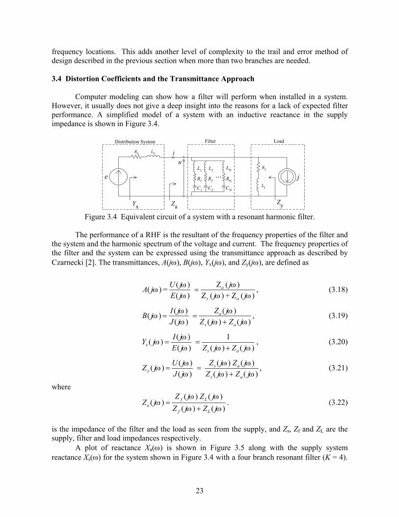
Computer modeling can show how a filter will perform when installed in a system.
However, it usually does not give a deep insight into the reasons for a lack of expected filter performance. A simplified model of a system with an inductive reactance in the supply impedance is shown in Figure 3.4.
Filter
LS
e
Distribution System
j
Load
YxZyZa
LL
RS
RL
ui
L1
...C1
R1
C2
R2
L2 LN
CN
RN
Figure 3.4 Equivalent circuit of a system with a resonant harmonic filter.
The performance of a RHF is the resultant of the frequency properties of the filter and
the system and the harmonic spectrum of the voltage and current. The frequency properties of the filter and the system can be expressed using the transmittance approach as described by Czarnecki [2]. The transmittances, A(jω), B(jω), Yx(jω), and Zy(jω), are defined as
Z ( )( )( ) =( ) Z ( ) + Z ( )
a
s a
jU jA jE j j j
ωωω
ω ω ω= , (3.18)
( )( )( ) ( ) ( ) ( )
a
s a
Z jI jB jJ j Z j Z j
ωωω
ω ω ω= =
+, (3.19)
( ) 1( )( ) ( ) ( )x
s a
I jY jE j Z j Z j
ωω
ω ω ω= =
+, (3.20)
( ) ( )( )( ) ( ) ( ) ( )
s ay
s a
Z j Z jU jZ jJ j Z j Z j
ω ωωω
ω ω ω= =
+, (3.21)
where ( ) ( )
( ) ( ) ( )f L
af L
Z j Z jZ j
Z j Z jω ω
ωω ω
=+
. (3.22)
is the impedance of the filter and the load as seen from the supply, and Zs, Zf and ZL are the supply, filter and load impedances respectively.
A plot of reactance Xa(ω) is shown in Figure 3.5 along with the supply system reactance Xs(ω) for the system shown in Figure 3.4 with a four branch resonant filter (K = 4).

24
For simplicity in this illustration the reactance, Xs, of the system inductance is assumed to be a linear function of frequency. From this plot it can be seen that the reactance Xa(ω) is capacitive in a frequency band below each tuning frequency.
Xa(ω) and Xs(ω), in per unit
Frequency (ω /ω1)
1
-1
ωa ωb ωc ωd
-Xs(ω)
Figure 3.5 Plot of reactance Xa and -Xs.
Therefore, a series resonance occurs at frequency ω = ωr when
( ) ( )s aX Xω ω= − . (3.23)
Thus, as shown in Figure 3.5, the resonant frequencies are at the points ωa, ωb, ωc and ωd where the plot of -Xs(ω) crosses the plot of Xa(ω). The system inductance shifts the frequency of the zeros of Xx(ω) with respect to Xa(ω) to lower frequencies. This is illustrated in the plot of reactance Xx(ω) shown in Figure 3.6. At such a resonance, the impedance seen by the supply Zx(jω) is equal to the resistance of the load with the filter, Ra(ωr), and the source resistance, Rs(ωr), namely
( ) ( ) ( )x r a r s rZ j R Rω ω ω= + . (3.24)
Xx(ω), in per unit
Frequency (ω /ω1)
1
-1
0ωa ωb ωc ωd
Figure 3.6 Plot of reactance as seen from the distribution voltage source e.
25
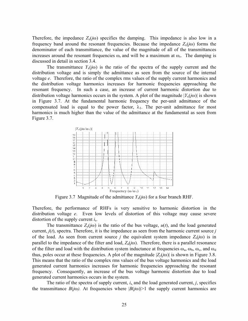
Therefore, the impedance Zx(jω) specifies the damping. This impedance is also low in a frequency band around the resonant frequencies. Because the impedance Zx(jω) forms the denominator of each transmittance, the value of the magnitude of all of the transmittances increases around the resonant frequencies ωr and will be a maximum at ωr. The damping is discussed in detail in section 3.4.
The transmittance Yx(jω) is the ratio of the spectra of the supply current and the distribution voltage and is simply the admittance as seen from the source of the internal voltage e. Therefore, the ratio of the complex rms values of the supply current harmonics and the distribution voltage harmonics increases for harmonic frequencies approaching the resonant frequency. In such a case, an increase of current harmonic distortion due to distribution voltage harmonics occurs in the system. A plot of the magnitude |Yx(jω)| is shown in Figure 3.7. At the fundamental harmonic frequency the per-unit admittance of the compensated load is equal to the power factor, λ1. The per-unit admittance for most harmonics is much higher than the value of the admittance at the fundamental as seen from Figure 3.7.
|Yx(jω /ω 1)|
Frequency (ω /ω 1) Figure 3.7 Magnitude of the admittance Yx(jω) for a four branch RHF.
Therefore, the performance of RHFs is very sensitive to harmonic distortion in the distribution voltage e. Even low levels of distortion of this voltage may cause severe distortion of the supply current is.
The transmittance Zy(jω) is the ratio of the bus voltage, u(t), and the load generated current, j(t), spectra. Therefore, it is the impedance as seen from the harmonic current source j of the load. As seen from current source j the equivalent system impedance Zs(jω) is in parallel to the impedance of the filter and load, Za(jω). Therefore, there is a parallel resonance of the filter and load with the distribution system inductance at frequencies ωa, ωb, ωc, and ωd thus, poles occur at these frequencies. A plot of the magnitude |Zy(jω)| is shown in Figure 3.8. This means that the ratio of the complex rms values of the bus voltage harmonics and the load generated current harmonics increases for harmonic frequencies approaching the resonant frequency. Consequently, an increase of the bus voltage harmonic distortion due to load generated current harmonics occurs in the system.
The ratio of the spectra of supply current, is, and the load generated current, j, specifies the transmittance B(jω). At frequencies where |B(jω)|>1 the supply current harmonics are

26
greater than the load generated current harmonics, and when |B(jω)|<1 the supply current harmonics are less than the load generated harmonics. Therefore, |B(jω)|=1 is the dividing line between bands of amplification and attenuation of harmonics in the supply current. This current harmonic amplification is the result of parallel resonance in the system.
A(jω) is the ratio of the spectra of bus voltage, u, and distribution voltage, e. Although, the A(jω) transmittance is numerically the same as the B(jω) transmittance, their meanings are different.
|Z y(jω /ω 1)|
Frequency (ω /ω 1) Figure 3.8 Magnitude of impedance Zy(jω) for a four branch RHF.
The amplification of voltage harmonics described by A(jω) is the result of series resonance. Because A(jω)=B(jω) the plot which shows the magnitude |A(jω)| is the same as for |B(jω)| and is shown in Figure 3.9.
|A(jω/ω1)| and |B(jω/ω1)|
Frequency (ω/ω1) Figure 3.9 Magnitude of the A(jω) and B(jω) transmittances for a four branch RHF.
However, only the values of these transmittances at each harmonic frequency are
needed to describe the effect of a transmittance at a particular harmonic. When the transmittances are evaluated only at harmonic frequencies nω1, they are referred to as
27
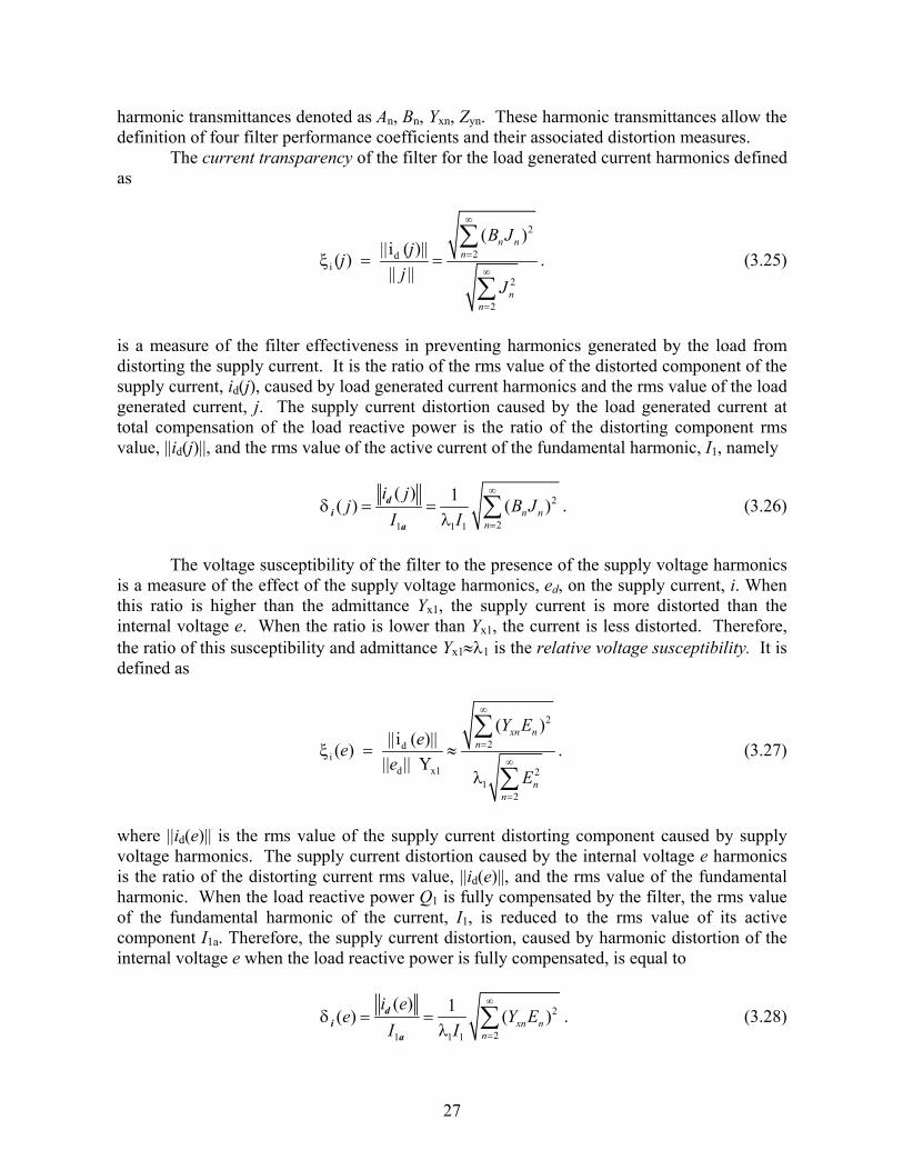
harmonic transmittances denoted as An, Bn, Yxn, Zyn. These harmonic transmittances allow the definition of four filter performance coefficients and their associated distortion measures.
The current transparency of the filter for the load generated current harmonics defined as
2
2di
2
2
( )||i ( )||( )|| ||
n nn
nn
B Jjj
jJ
ξ
∞
=
∞
=
= =∑
∑. (3.25)
is a measure of the filter effectiveness in preventing harmonics generated by the load from distorting the supply current. It is the ratio of the rms value of the distorted component of the supply current, id(j), caused by load generated current harmonics and the rms value of the load generated current, j. The supply current distortion caused by the load generated current at total compensation of the load reactive power is the ratio of the distorting component rms value, ||id(j)||, and the rms value of the active current of the fundamental harmonic, I1, namely
2
21 1 1
( ) 1( ) ( )n nn
i jj B J
I Iδ
λ
∞
=
= = ∑di
a
. (3.26)
The voltage susceptibility of the filter to the presence of the supply voltage harmonics
is a measure of the effect of the supply voltage harmonics, ed, on the supply current, i. When this ratio is higher than the admittance Yx1, the supply current is more distorted than the internal voltage e. When the ratio is lower than Yx1, the current is less distorted. Therefore, the ratio of this susceptibility and admittance Yx1≈λ1 is the relative voltage susceptibility. It is defined as
2
2di
d x1 21
2
( )||i ( )||( )
|| || Y
xn nn
nn
Y Eee
eE
ξ
λ
∞
=
∞
=
= ≈∑
∑. (3.27)
where ||id(e)|| is the rms value of the supply current distorting component caused by supply voltage harmonics. The supply current distortion caused by the internal voltage e harmonics is the ratio of the distorting current rms value, ||id(e)||, and the rms value of the fundamental harmonic. When the load reactive power Q1 is fully compensated by the filter, the rms value of the fundamental harmonic of the current, I1, is reduced to the rms value of its active component I1a. Therefore, the supply current distortion, caused by harmonic distortion of the internal voltage e when the load reactive power is fully compensated, is equal to
2
21 1 1
( ) 1( ) ( )xn nn
i ee Y E
I Iδ
λ
∞
=
= = ∑di
a
. (3.28)

28
The total supply current distortion is caused by both distorting currents, id(j) and id(e).
Harmonics of these currents that differ by their order n are mutually orthogonal, so that the square of the rms value of the sum of such harmonics is equal to the sum of squares of their rms value. Harmonics of the same order in both currents do not have any particular mutual phase relation, so that they add up as random quantities. Therefore, it can be assumed that their rms values add up with squares, and consequently, the supply current distortion can be expressed as
2 2
2 2
1 1
( ) ( )( ) ( )d dd
i i ia a
i j i eij e
I Iδ δ δ
+= = = + . (3.29)
The voltage transparency of the filter for distribution harmonics is the ratio of the
distorted bus voltage, ud(e), rms value and the rms value of the distorting component, ed, of the internal voltage, e, defined as
2
2
2
2
( )|| ( ) ||( )
|| ||
n nnd
ud
nn
A Eu ee
eE
ξ
∞
=
∞
=
= =∑
∑, (3.30)
It specifies the total effect of the distribution voltage harmonics on the distortion of the bus voltage. The bus voltage distortion caused by distortion of the internal voltage of the distribution system is equal to
2
2
1
( )( )
n nn
A Ee
Uδ
∞
==∑
u . (3.31)
The current susceptibility of the filter with respect to the bus voltage distortion is
defined as
0
|| ( ) ||( )|| ( ) ||
du
d
u jju j
ξ = . (3.32)
It is a measure of the effectiveness of the filter on the bus voltage distortion in the presence of the load current harmonics. Where ud(j) is the distorted voltage that occurs at the load terminals because of the current harmonics and udo(j) is the distorted voltage that occurs without the filter. Without the filter the bus voltage, udo(j), has the rms value

29
2 20
2 2( ) ( ) ( )d sn n sn n
n nu j Z I Z J
∞ ∞
= =
= ≈∑ ∑ , (3.33)
where the supply source impedance is much lower than the load impedance, so that In ≈ Jn. The filter changes this rms value to
2
2
( ) ( )d yn nn
u j Z J∞
=
= ∑ . (3.34)
The voltage distortion caused by the load generated current is the ratio of the rms value of the distorting component ud(j) and the rms value of the fundamental harmonic U1, therefore, it is equal to
2
2
1
( )( )
yn nn
u
Z Jj
Uδ
∞
==∑
. (3.35)
In order to find the total distortion of the voltage, similarly as in the case of distorting
current harmonics, harmonics of distorting voltages ud (j) and ud (e) are orthogonal or have random mutual phases. Therefore, the voltage distortion caused by both the distribution voltage harmonics and by the load generated current harmonics can be calculated approximately as the root of squares of the partial distortions δu(j) and δu(e), namely
2 2
2 2
1 1
( ) ( )( ) ( )d dd
u u u
u j u euj e
U Uδ δ δ
+= = = + . (3.36)
3.5 Effect of Damping
Attenuation of the load generated current harmonics to which a RHF is tuned improves with the decrease of the filter damping. Unfortunately, the harmful resonances of the filter with the distribution system increase in magnitude as damping declines. This indicates that effects of minor harmonics on the filter performance will increase with the increase of a filter’s quality factor (q-factor). In order to damp the filter resonance with the distribution system, an additional resistor is connected in each branch of filters studied in Ref. [19]. In another approach suggested in Ref. [1] a resistor is connected only when a resonant frequency is in close proximity to the 4th order harmonic frequency. Unfortunately, because the effect of damping on filter performance is opposite with respect to the attenuation of harmonics to which the filter is tuned and the attenuation of the minor harmonics, a trade-off results. The resultant effect depends on the proportion of these two groups of harmonics and cannot be predicted without a detailed study. Furthermore, there is a cost associated with damping in the form of extra loss of active power. The resonance is damped by the resistance of the filter branch, the resistance of the load and the resistance of the distribution system, as observed at the bus where the filter is installed. Unfortunately, these resistances depend on

30
frequency and their values are not easily available for the filter designer. Therefore, only an assessment of these resistances and the filter damping is possible. Such an assessment is presented below. 3.5.1 Maximum Harmonic Amplification
The transmittances A(jω) and B(jω), defined with formulae (3.18) and (3.19) can be re-written as
1( ) ( )
1 ( ) ( )a s
A j B jY j Z j
ω ωω ω
= =+
(3.37)
where Ya(jω) is the equivalent admittance of the filter and load, and is equal to
( ) ( ) ( )a a aY j G jBω ω ω= + . (3.38) If the effect of the load and filter resistance on the equivalent susceptance Ba(ωr) is neglected, then transmittances A(jω) and B(jω) at frequency ωr can be expressed as
1( ) ( )( )r r
ar sr ar sr sr ar
A j B jG R j G X R B
ω ω= =+ +
, (3.39)
where index r denotes the value at frequency ωr. Usually Rsr << Xsr, thus, the real part GarRsr of the denominator in the formula (3.39) can be neglected. Moreover, the equivalent conductance, Gar, is the sum of the filter conductance, GFr and the load conductance, GLr. Thus, the magnitude of transmittances, A(jωr) and B(jωr), denoted as Ar and Br, can be approximated by
1r r
sr ar Lr sr Fr sr
A BR B G X G X
= ≈+ +
. (3.40)
The formula (3.40) can be rearranged as
01
1r r rLr Fr
A B Ad d
= ≈+ +
. (3.41)
In this formula
0 01
r rsr ar
A BR B
= = , (3.42)
denotes harmonic amplification at a resonant frequency, ωr, in the lack of resonance damping by the load and the filter resistance, i.e., when GFr = 0 and GLr = 0. This is the maximum

31
harmonic amplification possible at the bus when the load is reactive and the filter has an infinite q-factor. The coefficient
sr LrLr
sr ar
X GdR B
= , (3.43)
specifies the resonance damping due to the load resistance, while the coefficient
sr FrFr
sr ar
X GdR B
= , (3.44)
specifies the resonance damping due to the filter resistance.
The maximum possible harmonic amplification Ar0 at resonant frequency depends on the equivalent resistance of the distribution system Rs at frequency ωr. For a rough approximation it can be assumed that its value is the same as for the fundamental harmonic and can be calculated from the formula
2
21sr s
sc s
UR RS ξ
≈ =+
, with ss
s
XR
ξ = . (3.45)
The equivalent susceptance Ba is a sum of the filter and load susceptance. The load
susceptance at frequency ωr is equal to
2 2
1 tan1 tanLr
L
rBR r
ϕϕ
= −+
. (3.46)
where RL = U2λ2/P, ϕ = cos-1(λ) and r = ωr/ω1. For ωr >> ω1 and common values of the power factor λ, this susceptance can be approximated by
2 2
1 1tan 1
LrL
PBR r r Uϕ λ λ
= − = −−
. (3.47)
thus, its magnitude declines monotonically as the resonant frequency ωr increases. The filter susceptance BFr is the second component of the equivalent susceptance, Bar. The effect of the branch resistance, Rk, on the branch susceptance, Bkr for the resonant frequency
1Im Im 1kr kr
k r kr k
B YR j L
j Cω
ω
= =+ +
(3.48)
is usually negligible, therefore, the filter susceptance is approximately equal to

32
21 1 1
k K k Kr k
Fr krk k r k k
CB BL C
ωω
= =
= =
= ≈−∑ ∑ , (3.49)
If Ωk denotes tuning frequency of the k-th branch, then, taking into account formula (3.7), the filter susceptance can be expressed as
2
12 2 21
1Kk
Fr kk k
rB h QU r
ζζ=
−≈
−∑ , with 1
kkζ
ωΩ
= (3.50)
Illustration: A reactive load at the supply voltage assumed to be U = 1 pu and the
apparent power S = 1 pu is supplied from a bus with the short circuit power Ssc = 30 pu and the reactance to resistance ratio ξs = Xs/Rs = 5. The filter is tuned to the 5th and 7th order harmonics and each branch compensates a half of the load reactive power, dk=0.5. As shown in Fig. 3.10, the resonant frequencies are approximately equal to ωr = 3.97 ω1 and 6.05 ω1.
|A(jω)|, |B(jω)|
q= ∞
q= ∞
q=100
q=100q=30
q=30ω /ω1
Figure 3.10 Effect of q-factor on A(jω) and B(jω).
For the circuit parameters as assumed, the distribution system has the equivalent resistance, calculated from formula (3.45), equal to Rs = 0.0065 pu. The load and the filter susceptance are compiled in Table 3.1. These values show that the load susceptance has a relatively low effect on the maximum value of harmonic amplification. Moreover, the relatively low difference between harmonic
Table 3.1 Load and filter susceptance in the circuit
ωr rd/sec 3.97 6.05 BLr pu - 0.25 - 0.16 B1r pu 5.19 - 6.26 B2r pu 2.89 11.71 BFr pu 7.83 5.29 Ar0 -- 19.6 29.1

33
amplification calculated and its value obtained from a computer modeling justifies the simplifications assumed in this section. 3.5.2 Damping by the Filter and Load
The load related damping coefficient, dLr, specified with formula (3.43), can be rearranged as follows
sr LrLr s Lr
sr ar ar
X G rd GR B B
ξ= = , (3.51)
where the load conductance at resonant frequency is equal to
2 2 2 2 2
1 1 11 tan (1 )Lr
L
PGR r r Uϕ λ
= ≈+ −
. (3.52)
The filter related damping coefficient, dFr, specified with formula (3.44) can be expressed as
1
k K
Fr s Fr s krkar ar
r rd G GB B
ξ ξ=
=
= = ∑ , (3.53)
where the conductance at frequency ωr of the filter branch tuned to frequency Ωk is equal to
2
2 2 2
( )1
[1 ( ) ] ( )
r k kkr
rkr k k
k
R CGR R C
ωω
ω=
− +Ω
. (3.54)
Since
21( ) 1 ( )r rr k k
k k k
R Cq
ω ωω = << −
Ω Ω, (3.55)
conductance Gkr is approximately equal to
2
1
( )
k kkr
k r k
r k
CGqω
ω
Ω≈
Ω−
Ω
(3.56)
where qk is the branch q-factor at the tuning frequency, Ωk,
k kk
k
LqR
Ω= . (3.57)

34
The conductance of the filter branch can be expressed in terms of the branch reactive power, namely, it is equal to
1
12
2
1
( )
k
k kkr
k r k
r k
QGU q
ωω
ωω
Ω−
Ω≈
Ω−
Ω
(3.58)
An investigation of formulae for load and filter damping coefficients (3.51) and (3.53)
shows, that as long the reactance to resistance ratio, ξs, remains constant, the load and filter resonance damping coefficients remains independent of the supply short-circuit power, Ssc, which on other hand affects the resonant frequencies, ωr.
Illustration: The load and filter resonance damping coefficients are evaluated for a reference load, specified in per unit, namely, such a load that the voltage U = 1 pu, ω1 = 1rd/sec, the active power P = Q = 1 pu, thus, the PF equal to λ =0.707. The reactance to resistance ratio at the bus is assumed to be ξs = Xs/Rs = 5. The filter has two branches, tuned to the 5th and 7th order harmonics, thus Ω1 = 5 rd/sec, Ω2 = 7 rd/sec, and the same reactive power, Q1/2. The damping coefficients are calculated for two resonant frequencies that coincide with the 4th and the 6th order harmonics and for two different q-factors, the same for each branch, namely, q = 100 and q = 30. The conductance and susceptance of the load and the filter branches for resonant frequencies are compiled in Table 3.2. The results compiled show that for a common level of the filter q-factor, the load resistance has much lower contribution to the resonance damping than the filter resistance.
Table 3.2 Conductance and susceptance of the load and the filter branches for resonant frequencies.
ωr rd/sec 4 6 GLr pu 0.125 0.041 BLr pu - 0.50 - 0.286 B1r pu 5.33 - 6.54 B2r pu 2.91 11.08 Bar pu 7.74 4.25 dLr - 0.32 0.29 q - 100 30 100 30
G1r pu 0.119
0.396
0.179
0.596
G2r pu 0.025
0.083
0.358
1.19
GFr pu 0.144
0.479
0.537
1.79
dFr pu 0.37 1.24 3.79 12.6

35
Also, they show that the lowest resonance is much less damped than the resonance at higher frequencies. This confirms the earlier conclusion, that the lowest resonance is much more crucial for the filter performance than resonances at higher frequencies.
Observe, that according to formulae (3.42) and (3.53) both the maximum harmonic amplification Ar0 and the filter resonance damping coefficient depend on the equivalent susceptance, Bar. However, when
dFr >> 1+ dLr (3.59)
the harmonic amplification at resonant frequency can be approximated by
0 1 1rr
Fr s s Fr s Fr
AAd rR G r X Gξ
= = = (3.60)
thus, becomes independent on the filter and the load susceptance.
The resonance of the filter with the distribution system causes not only resonant amplification of the voltage and current harmonics. This resonance also changes the admittance as seen from the distribution system as well as the impedance as seen by the load generated harmonic currents, specified by the transmittances (3.20-3.21). At resonant frequencies this admittance and impedance may approach a very high value.
In the lack of the resonance damping by the filter and load resistance, the magnitude of admittance Yx(jω) at the resonant frequency, ωr, has a maximum value, denoted by Yxr0. The resonant current is bounded only by the distribution system resistance, Rs, hence
0 1/xr sY R= . (3.61)
The effect of the load and the filter resistance on the resonance admittance, Yxr, can be evaluated, assuming that the equivalent conductance Gan is much lower than susceptance Ban, using formula which is similar to formula (3.41) for the resonant harmonic amplification, namely,
01
1xr xrLr Fr
Y Yd d
≈+ +
, (3.62)
where coefficients dLr and dFr are defined with formulae (3.43) and (3.44). An example of the plot of the magnitude of admittance Yx(jω) dependence on q-factor is shown in Fig. 3.11. This plot was drawn for a system where a two branch RHF tuned to the 5th and 7th order harmonics is connected at a bus with short circuit power 40 times higher than load active power P. The power factor λ = 0.707 and the ratio Xs/Rs = 5.
At the resonant frequency, ωr, the impedance Zy(jω) = Zyr is equal to
( )sr sr
yras sr sr ar Lr sr Fr sr
R jXZG R j R B G X G X
+=
+ + +. (3.63)

36
|Yx(jω)|
ω /ω1
q = 100
q = ∞
q = ∞q = 100
q = 30
q = 30
Figure 3.11 Effect of damping on admittance Yx(jω) magnitude.
Since typically
sr s sr sR R X rX≈ << ≈ , (3.64)
impedance Zyr can be approximated as
01
1yr yrLr Fr
Z Zd d
≈+ +
, (3.65)
where
0sr s
yrsr ar ar
XZ rR B B
ξ= = . (3.66)
The impedance Zyr0, and consequently the bus voltage distortion caused by the load generated current harmonics jn increases with the resonance frequency increase and with increase in the reactance to resistance ratio ξs,. This impedance also depends on the susceptance Bar, which is, however, a complex function of frequency. This impedance drawn for a system with the same parameters as used in Fig. 3.11 is shown in Fig. 3.12. 3.5.3 Damping Effect on Distortion and Active Power Loss
It is evident that the reduction of the q-factor, reduces the magnitude of transmittances A(jω), B(jω), Yx(jω) and Zy(jω) at resonant frequencies, ωr,. Unfortunately, the reduction of the q-factor increases the magnitude of these transmittances for the tuning frequencies of the filter, and this is less visible. Consequently, the reduction of the filter q-factor affects the minor harmonics and the harmonics to which the filter is tuned in an opposite way. The resultant effect depends on the voltage and current spectra and on the frequencies of the filter resonance with the distribution system. If such a resonance coincides with the frequency of a minor harmonic, the reduction of the q-factor may reduce the waveform distortion. Otherwise, the distortion may increase.

37
|Zy(jω)|
q = ∞
q = ∞
q = 100 q = 100 q = 30 q = 30 ω /ω1
Figure 3.12 Effect of damping on impedance Zy(jω) magnitude.
When an auxiliary resistor is not connected in a filter branch it has a q-factor
dependent only on the inductor reactance and resistance at the resonant frequency. Such a q-factor will be referred to as a natural q-factor. Depending on the inductor construction, power ratings and frequency, the natural q-factor is usually of the order of 50-200 or even higher. Reduction of the q-factor below its natural value requires that an additional resistor be connected in the filter branch. This resistor increases the active power loss in the branch, and consequently, increases the operational cost of the filter. Unfortunately, a multiple-branch filter, when operated in the presence of several current harmonics generated in the load and several distribution voltage harmonics, is too complex for an analytical study. Computer modeling, although it provides results only for a case by case basis, enables us to draw some conclusions concerning the effect of the q-factor on the filter performance and the active power loss.
As can be seen in Figs. 3.10-3.12, the reduction of the q-factor reduces the magnitude of transmittances A(jω), B(jω), Yx(jω) and Zy(jω) substantially only in the vicinity of the resonant frequency. Therefore, one could expect, that in a situation when resonant frequencies are sufficiently far from harmonic frequencies, then the q-factor value does not have any substantial effect on the filter performance. It would be a wrong conclusion, however, since the q-factor affects transmittances A(jω), B(jω), Yx(jω) and Zy(jω) value at tuning frequencies. This value increases with the q-factor reduction and consequently, filter effectiveness declines. This is shown in the following illustration.
Illustration: Let us consider the same bus, load and RHF as previously with a two branch RHF tuned to the 5th and 7th order harmonics, Ssc=40, λ = 0.707 and the ratio Xs/Rs = 5. The load generates the 5th and 7th order current harmonics of the RMS value J5 = 18% and J7 = 11% of the fundamental and a uniform harmonic of the RMS value J2 = J3 = J4 = J6 = 0.2%. The minor harmonics of the frequency above the highest tuning frequency do not have substantial effect on the filter performance and are neglected. As to distribution voltage distortion, it was assumed that it contains a uniform harmonic noise on the level of En = 0.1% of the fundamental. The dependence of the coefficients of the current and voltage distortion as well as the active power loss, ∆P, in the filter on the q-factor in the range from q = 10 to q = 100 are shown in Fig. 3.13. Level 10 in the figure represents the level of distortion and the power loss maximum values.

38
The minimum and maximum values of distortion coefficients and the active power loss in the filter, in per cent of the load active power, are compiled in Table 3.3.
Table 3.3 Distortion coefficients and the active power loss in the filter.
q δi(j) δi(e) δu(j) δu(e) ∆P
10 8.3 2.6 1.06 0.36 2.4 100 1.7 3.4 0.20 0.49 0.24
As can be seen from Fig. 3.13, the bus voltage distortion caused by the distribution voltage harmonics declines with the q-factor reduction. It can be attributed to the reduction in the magnitude of admittance Yx(jω) along with the q-factor decline. This reduction in is very low, however, when it is compared with in the increase in the distortion caused by the load current harmonics. This is because the system becomes more transparent for the current harmonics to which the filter is tuned with the q-factor decline. Reducing q-factor in such a situation degrades the filter performance along with a substantial increase of the active power loss in the filter. This situation may change with an increase in the distribution voltage distortion and when resonant frequency coincides with a harmonic frequency.
δi(e)
δu(e)
δi(j) δu(j) ∆P q
Figure 3.13 Distortion coefficients and active power loss versus q-factor.
Finally, consider the same system with the same load current and distribution voltage harmonics as above, except with the supply rating reduced to Ssc = 30 pu. In this case the resonant frequencies are now very close to the frequencies of the 4th and the 6th order harmonics. The minimum and maximum values of distortion coefficients and the active power loss in the filter are compiled in Table 3.4.
Table 3.4 Distortion coefficients and the active power loss in the filter
q δi(j) δi(e) δu(j) δu(e) ∆P
10 6.3 3.3 1.1 0.47 2.4 100 3.5 9.5 0.51 1.3 0.24

39
The plot of coefficients of the current and bus voltage distortion, calculated according to formulae (3.29) and (3.36), as the function of the q-factor, q, is shown in Fig. 3.14.
δu
δi
∆P
q
Figure 3.14 Distortion and active power loss versus q-factor. These coefficients have a minimum at the q-factor approximately equal to 20. Thus, reduction of the amplification of the 5th and the 7th order harmonics and the system admittance Yx(jω) with the q-factor, reduction enables us to improve the filter effectiveness in such a situation. Unfortunately, this improvement is accompanied by a substantial increase in the active power loss.

40
Chapter 4
Fixed-Pole Resonant Harmonic Filters 4.1 Introduction
Because of the sensitivity of the conventional RHF to supply voltage distortion, a
modification of the filter structure, which would reduce this sensitivity is needed in cases where voltage distortion reduces effectiveness of conventional RHFs below an acceptable level. The sensitivity can be reduced by the addition of a line inductor to the filter as suggested in [2]. Such a line inductor added between the point of common supply and a conventional RHF is shown in Figure 4.1. The sensitivity of the filter to distribution voltage distortion is reduced by the line inductor because it reduces the admittance as seen by the distribution system.
The presence of the line inductor, L0, makes possible the design of the filter in such a way that frequencies of poles, that means the frequencies of harmful resonances of the filter with the distribution system inductance, are selected at the designer’s discretion. Because these poles are fixed at the beginning of the filter design and this is an important property of the filter characteristic, such filters are termed fixed-pole RHFs. As shown in section 3.3, for conventional filters the frequencies of these poles are not known until the filter is designed and modeled. A fixed-pole filter could be considered as a conventional RHF with a line inductor, but designed in a special way that enables the designer to fix harmful resonances at selected frequencies.
LinearLoad
e
i PCS
RHF
Lo
HGL
Figure 4.1 Distribution System with a RHF and series inductor L0.
Because the line inductor, L0, is connected in series with the equivalent inductance, Ls,
of the distribution system, it increases the inductance as seen from the RHF and reduces its relative variability due to the system reconfiguration. Therefore, fixed-pole RHFs have a reduced sensitivity of location of poles to changes of the distribution system parameters.
The fixed-pole RHFs enable [2] an increase in the effectiveness of harmonic sup-pression, unfortunately at the cost of reduction of the short circuit power at the PCS. This results in higher fluctuation of the load voltage rms value with change of the load power. However, as discussed in section 2.4.3, the use of additional line inductance for low pass

41
filtering is becoming more common. This indicates that additional line inductance is now considered to be acceptable for filtering purposes despite the reduction in short circuit power. 4.2 Synthesis of Fixed-Pole Resonant Harmonic Filters
The fixed-pole filter allows harmful resonance conditions to be avoided by specifying pole locations that do not coincide with harmonic frequencies. The most simple approach to avoid such a resonance is to locate poles equidistant to neighboring harmonic frequencies. For example, if filter is tuned to the 5th and 7th order harmonics, a pole can be located at frequencies 5.5ω1 or 6.5ω1. This simple example shows that a criterion is needed for the selection of pole locations.
The distribution system, the filter and the load at the PCS can be considered as one-ports. The synthesis method developed in [2] assumes that these one-ports are loss-less, and therefore they are reactance one-ports. This assumption may result in a substantial error at the fundamental frequency, but can provide acceptable results at higher order harmonics for which the filter parameters are calculated. At such an assumption the distribution system impedance is approximated by the reactance of an inductance, Ls, while the load impedance is approximated by the reactance of an inductance L1e, equivalent with respect to the load reactive power Q1 at the fundamental frequency. The single phase equivalent circuit of a distribution system, four branch fixed-pole RHF and the load, approximated as reactance one-ports is shown in Figure 4.2.
Since the main application of RHFs is the reduction of distortion caused by three-phase, six pulse rectifiers or ac/dc converters that generate harmonics of the order n = 6k ± 1, that means the 5th, 7th 11th 13th, 17th,…. and usually four branch filters are used for that purpose, considerations here are confined to just such RHFs, i.e. tuned to the 5th, 7th 11th 13th order harmonics.
ub
L1e
LS
C3C2
L1
C1
L3 L4L2
C4
L0PCS
ZaYx
e
Figure 4.2 Equivalent circuit of distribution system, load and fixed-pole RHF.
The impedance Za of the shunt branches in parallel with the load equivalent inductance, has four zeros due to the series resonance of each tuned branch at complex frequencies s = jz1, jz2, jz3, jz4. If the filter fully compensates the load reactive power at the fundamental frequency, that means impedance Za at the fundamental is infinite, thus there is a pole at s = j1 rad/s. Moreover, due to the filter and the load structure as shown in Fig. 4.2, it is an open circuit at infinite frequency and consequently, the impedance Za has a pole at infinity. Because each pair of zeros of a reactance one-port has to be separated by a single pole, [51, 52], as shown in Figure 4.3,

42
Figure 4.3 Plot of impedance Za(jω).
therefore, impedance Za should have the form
( )( )( )( )( )( )( )( )
2 2 2 2 2 2 2 21 2 3 4
2 2 2 2 2 2 21 2 3
( )1a
s z s z s z s zZ s As
s s b s b s b
+ + + +=
+ + + + (4.1)
where the complex value, s = jbk, denotes pole and A is a positive real number.
Because one goal of the fixed-pole filter is to reduce the sensitivity to supply voltage distortion, the magnitude of the admittance seen by the supply, Yx, is critical. Therefore, poles of interest are the poles of the input admittance, Yx. The locations of these poles are the frequencies at which the sum of the impedance Zx and Za are equal zero. A plot of the reactance function Za(jω) and the impedance -Zx(jω), which is a function of the supply inductance in series with added inductance L0, are shown in Figure 4.4.
Figure 4.4 Plot of impedances Za(jω) and -Zx(jω).

43
This plot clearly shows the pole locations which are at the intersection of the plot of -Zx(jω) and the regions where Za(jω) has a capacitive impedance. These are also the frequencies of the poles of the impedance as seen by the load generated current harmonics, therefore, these points of intersection on the plot are denoted as poles p1, p2, p3 and p4.
Selecting these four pole locations yields the following set of four equations
1 1 0 1
2 2 0 2
3 3 0 3
4 4 0 4
( ) 0( ) 0( ) 0( ) 0
s a
s a
s a
s a
p L p L Z pp L p L Z pp L p L Z pp L p L Z p
+ + =+ + =+ + =+ + =
(4.2)
or simply
0 ( ) 0k s k a kp L p L Z p+ + = (4.3)
with k = 1, 2, 3, 4. To solve the above system of equations it is more convenient to express Za(s) as
( )( )( )( )( )( )2 2 2 2 2 2 2 2
1 2 3 4
2 6 4 23 2 1 0
( )1a
s z s z s z s zZ s s
s a s a s a s a
+ + + +=
+ + + + (4.4)
There are only four equations and five unknown variables, namely, a3, a2, a1, a0 and L0. However, as s approaches zero, the impedance Za(s) approaches sL1e, such that
1s 0lim ( )a eZ s sL→
= , (4.5)
and the impedance given in eqn. (4.3) as s approaches zero gives
21 2 3 4
00
( )lim ( )as
z z z zZ s sa→
= . (4.6)
Therefore, the coefficient a0 is equal to
( )21 2 3 4
01e
z z z za
L= . (4.7)
The equation (4.3) results in real, positive coefficients a3, a2, a1, and L0 on the condition [51] that a single pole is located between each pair of zeros of the impedance (4.4) as well as at infinity. If these coefficients are known then the impedance Za(s) of the filter is also known. Thus, the circuit elements of the filter can be calculated. The inductance of each of the four branches is equal to

44
2 2lim ( )k
k as jzk
sL Z ss z→
= +
, (4.8)
and the capacitance is equal to
2
1k
k k
Cz L
= , (4.9)
where k = 1, 2, 3, 4. 4.3 Effect of Poles Selection on the Line Inductor
The zeros jz1, jz2, jz3, jz4. and poles jp1, jp2, jp3, jp4. of the impedance Za(s) are selected at the designer’s discretion. The required line inductance L0 is an implicit function of these zeros and poles. For a filter that has to eliminate particular load current harmonics, the zeros are fixed. Thus, only poles can be selected.
The line inductance L0 affects both the load and the filter performance. At a high value of this inductance, the load voltage would change with the load power variation. At a low value, the filter performance would be affected by reconfigurations in the distribution system. Therefore, it is one of the most important parameters of the fixed-pole filter. Although it can be found as a solution of equations (4.3), it would be useful to have an explicit formula for its calculation and its dependence on the poles selection.
The dependence of the inductance L0 on the filter poles can be developed as follows. For s = jpk equation (4.3) can be expressed in the form
( ) ( )( )( )( )( )
26 4 2
3 2 1 0 2 2 2 2 2 2 2 21 2 3 4
1 1 0kk k k
xk k k k
pp a p a p a a
Lz p z p z p z p
−− + − + + =
− − − − (4.10)
where k = 1, 2, 3, 4, represents the shunt branch number and, therefore, the index of the pole. The inductance Lx = Ls + L0, is the sum of the supply inductance and the line inductance. Let us denote
2
2 2 2 2 2 2 2 21 2 3 4
1( )( )( )( )
kk
k k k k
p bz p z p z p z p
−=
− − − − (4.11)
so that, equation (4.10) could be rearranged as follows
( )6 4 23 2 1 0
1k k k k k
x
p a p a p a b a bL
− + − + = − (4.12)
With the right-side coefficient denoted as
0k kc a b= − , (4.13) the equation (4.12) can be expressed in matrix form as

45
1 1
11 2 2
3 3
21 4
1111 1/ x
a cB a c
a cB L c
=
, (4.14)
where
6 4 21 1 1 1 1 16 4 2
11 2 2 2 2 2 26 4 23 3 3 3 3 3
p b p b p bB p b p b p b
p b p b p b
− − = − − − −
(4.15)
and
6 4 221 4 4 4 4 4 4B p b p b p b = − − . (4.16)
Multiplying both sides by the matrix
121 11
I 0-B IB−
(4.17)
yields
1
21
11 12 32
131 1
22 21 11 12 4 21 11 2
3
0 ( ) 1/ x
cca
B B caca
B B B B c B B cLc
− −
= − −
, (4.18)
therefore, the inductance Lx has a value given by
[ ]
122 21 11 12
T14 21 11 1 2 3
xB B B BL
c B B c c c
−
−
−=
−. (4.19)
Multiplying the matrix expression in the denominator yields
4 42 2
11 1
42 2 2 2 21 2 3 4
1
(1 ) ( 1 )
(1 )(1 )(1 )(1 )
e p p p k z z z kk k
x
kk
L e f g z e f g pL
p p p p z
= =
=
− − + − + − + − +
=− − − −
∏ ∏
∏ (4.20)

46
where
2 2 2 21 2 3 4
2 2 2 2 2 21 2 1 3 1 4 2 3 2 4 3 4
2 2 2 21 2 3 1 2 4 1 3 4 2 3 4
( ) ( ) ( ) ( ) ( ) ( )
( ) ( ) ( ) ( )
p
p
p
e p p p p
f p p p p p p p p p p p p
g p p p p p p p p p p p p
= + + +
= + + + + +
= + + +
(4.21)
and, similarly,
2 2 2 21 2 3 4
2 2 2 2 2 21 2 1 3 1 4 2 3 2 4 3 4
2 2 2 21 2 3 1 2 4 1 3 4 2 3 4
( ) ( ) ( ) ( ) ( ) ( )
( ) ( ) ( ) ( )
z
z
z
e z z z zf z z z z z z z z z z z zg z z z z z z z z z z z z
= + + +
= + + + + +
= + + +
(4.22)
Formula (20) could be simplified to
21 2 3 4
12 2 2 21 2 3 41 2 3 4
11 [ ( ) ]1( 1)( 1)( 1)( 1)p p pz z z
x ez z z
g f eg f e p p p pL Lg f e z z z zp p p p− + −− + −
= −− + −− − − − (4.23)
and then expressed as
21 2 3 412 2 2 2
1 2 3 41 2 3 4
1 ( ) ( 1)( 1)( 1)( 1)( 1)
pz z zx e
z
Ag f e p p p pL Lz z z z Ap p p p− + −
= −− − − −
(4.24)
where
2 2 2 2 21 2 3 4 1 2 3 4
2 2 2 2 2 2
1 2 1 3 1 4 2 3 2 4 3 4
2 2 2
1 2 3 1 2 4 1 3 4
1 1 1 1 1( )
1 1 1 1 1 1 ( ) ( ) ( ) ( ) ( ) ( )
1 1 1 ( ) ( ) ( )
p p pp
g - f +e -A
p p p p p p p p
p p p p p p p p p p p p
p p p p p p p p p
= = + + + −
− − − − − − +
+ + + + 2
2 3 4
2
1 2 3 4
1( )
1 ( )
p p p
p p p p
+
−
(4.25)
and

47
2 2 2 2 21 2 3 4 1 2 3 4
2 2 2 2 2 2
1 2 1 3 1 4 2 3 2 4 3 4
2 2 2
1 2 3 1 2 4 1 3 4
1 1 1 1 1( )
1 1 1 1 1 1 ( ) ( ) ( ) ( ) ( ) ( )
1 1 1 ( ) ( ) ( )
z z zz
g - f +e -Az z z z z z z z
z z z z z z z z z z z z
z z z z z z z z z
= = + + + −
− − − − − − +
+ + + + 2
2 3 4
2
1 2 3 4
1( )
1 ( )
z z z
z z z z
+
−
(4.26)
Since for RHFs p1 < p2 < p3 < p4 then ep << fp << gp, therefore, the term Ap can be approximated by
2 2 2 21 2 3 4
1 1 1 1pA
p p p p≈ + + + . (4.27)
Similarly, Az can be approximated by
2 2 2 21 2 3 4
1 1 1 1zA
z z z z≈ + + + . (4.28)
Therefore, inductance Lx is approximated by
0 ( 1)px s
z
AL L L d A= + ≈ − (4.29)
where 21 2 3 4
1 2 2 2 21 2 3 4 1 2 3 4
1 ( )( 1)( 1)( 1)( 1)
z z ze
p p p pg f ed Lp p p p z z z z
− + −=
− − − − (4.30)
Although approximations (4.27) and (4.28) reduce the complexity considerably,
equation (4.29) still does not allow the relation between inductance Lx and the choice of filter poles and tuning frequencies to be easily seen. However, one further assumption that will simplify the problem can be made. In general, the tuned frequencies, i.e. the zeros, are fixed, thus Az is a constant and inductance Lx depends only on the location of the poles. Also, as seen by examination of (4.30), d is only slightly affected by changes in the pole locations as compared to Ap, i.e. it is nearly constant. Therefore, it can be seen by observing only Ap in (4.29) that inductance Lx declines in value with the increase of any pole frequency. This means that at some selection of poles which yields Lx = Ls, it becomes necessary to decrease the frequency of one or more poles in order to increase the frequency of any other pole, since otherwise the minimum value of L0 = 0 would be violated. Furthermore, the approximation (4.27) shows that Ap is the most affected by poles located at the lowest frequencies, p1 and p2. Therefore, consider an illustration where p3 and p4 are fixed. Given a system with L1e = 1.4 pu, Ls = 0.033pu, and a typical filter tuned to 5th, 7th, 11th, and 13th order harmonics, the inductance L0 as a function of p1 and p2 with chosen poles of p3 = 9.5 and p4 =12.5 is

48
2 2 21 2 2
0 2 21 2
(1.425 0.1125 ) 1.425 0.033( 1)( 1)
p p pLp p
− + −=
− − (4.31)
The surface plot of L0 versus poles p1 and p2 in Figure 4.5 below shows that the inductance L0 declines to a negative value. This illustrates that the increase of either pole or both will result in a declining value of L0. This is in agreement with the earlier conclusion respective equation (4.29), and the greater effect of p1can be observed by the greater decline along the p1 axis in the plot. It also shows that as pi approaches zi where i = 1,2,3,4, then Lx approaches 0. This can be concluded intuitively by examination of the plot of impedances Za and Lx.
3 3.5 4 4.55p1
5.56
6.570
0.050.1
3 3.5 4p2
L0
Figure 4.5 Plot of L0 as a function of filter poles p1 and p2.
Finally, if we express equation (4.29) as a function of p1 where all other poles are at the maximum theoretical values, p2 = 7, p3 = 11 and p4 =13, then it becomes
21
0 21
1.454 0.0851
pLp−
=−
. (4.32)
Because the selected values of the other poles are at the locations that yield the smallest value of L0, this enables us to determine the maximum value of p1 that would allow the selection of all other poles within their full possible range. For this example, if p1 ≤ 4.10 then any values of the other poles may be selected for L0 ≥ 0, of course, with the usual restriction that each pole must occur between a pair of zeros. A plot of L0 versus p1 is shown in Figure 4.6. In addition to the restriction on the minimum value of L0, there should also be an upper bound on the value of inductance L0, (L0)max, which is determined by the minimum short circuit power that can be tolerated in a particular system. In order find the possible selections of poles that yield a value of inductance in the range 0 < L0 < (L0)max it is convenient to simplify (4.30) as
21 2 3 41 12 2 2 2 2
1 2 3 4 1 2 3 4 1 2 3 4
1 1( )( 1)( 1)( 1)( 1) ( )
z z z z z ze e
p p p pg f e g f ed L Lp p p p z z z z z z z z
− + − − + −= ≈
− − − − (4.33)

49
where d is now a constant.
3.5 4 4.5 5p1
-0.02
0.02
0.04
0.06
0.08
L0
Figure 4.6 Plot of L0 as a function of p1 Observe that the lowest pole, p1, could be assumed to be equal to 3.5, and in such case neglecting one as compared to p1
2 could cause an error of the order of 10 percent. Thus, the line inductance is approximately equal to
0 ( 1)ps
z
AL d LA≈ − − . (4.34)
Since 0 < L0 < (L0)max
2 2 2 21 2 3 4
0 max
1 1 1 1
0 ( 1) ( )sz
p p p pd L LA
+ + +< − − < (4.35)
where (L0)max can be selected at the designer’s discretion. This formula can be modified to
0 max
2 2 2 21 2 3 4
1 1 1 1 ( )( 1) ( 1)s sz z
L L LA Ad dp p p p+
+ < + + + < + (4.36)
and finally written in the form
2 21 22 2 2 2
1 2 3 4
1 1 1 1r rp p p p
< + + + < (4.37)
where
2 2 0 max1 2
( )( 1) and ( 1)s sz z
L L Lr A r Ad d
+= + = + (4.38)
This is the equation of a ring of radiuses r1 and r2 in four-dimensional space. This ring confines the selection of poles of the filter. Since the poles at the highest frequency, p3 and p4

50
have the least contribution to inequality (4.37), they could be fixed. This reduces the equation of the ring in four-dimensional space to two-dimensional space, namely.
2 21 22 2
1 2
1 1( ') ( ')r rp p
< + < (4.39)
where 2 2
1 1 2 23 4
1 1( ')r rp p
= − − and 2 22 2 2 2
3 4
1 1( ')r rp p
= − − . (4.40)
In general the best choices for pole locations will be in a frequency range centered
around frequencies which are in-between adjacent harmonic frequencies. Therefore, table 4.1 below gives possible value that could be selected for the filter poles if the poles’ locations are restricted to be equidistant respective to adjacent harmonic frequencies.
Table 4.1 Possible pole selections.
Set #
p1
ω /ω1 p2
ω /ω1 p3
ω /ω1 p4
ω /ω1
1 3.5 5.5, 6.5 7.5, 8.5, 9.5, 10.5
11.5, 12.5
2 4.5 5.5 7.5, 8.5,9.5, 10.5
11.5, 12.5
3 4.5 6.5 7.5
11.5
4.4 Properties of Fixed-Pole RHFs
Although properties of conventional and fixed-pole filters are essentially very similar, the fixed-pole filters have reduced sensitivity to distribution voltage distortion. Similarly, as for the conventional RHF, the transmittance approach provides insight into the reasons for the behavior or performance level of the filter. Although the transmittances, A(jω), B(jω), Yx(jω), and Zy(jω), can also be used to describe the frequency characteristics of the fixed-pole filter, they are not the same as those for the conventional RHF. Fixed-pole RHF transmittances are modified by the addition of the series inductor, and are equal to
0
0
=( ) ( )
( ) ( )( )( )( ) ( )
a
s aj j
Z j Z jU jA jE j Z Z j Zω ω
ω ωωω
ω ω=
+ +
+ , (4.41)
0
( )( )( ) ( ) ( ) ( ) ( )
a
s a
Z jI jB jJ j Z j Z j Z j
ωωω
ω ω ω ω= =
+ +, (4.42)
0
( ) 1( )( ) ( ) ( ) ( )x
s a
I jY jE j Z j Z j Z j
ωω
ω ω ω ω==
+ +, (4.43)
0
( ) ( )( )( )
( ) ( ) ( ) ( )s a
ys a
Z j Z jU jZ jJ j Z j Z j Z j
ω ωωω
ω ω ω ω==
+ +, (4.44)

51
where ( ) ( )
( ) ( ) ( )b L
ab L
Z j Z jZ j
Z j Z jω ω
ωω ω
=+
. (4.45)
is the impedance of the shunt branches of the filter and the load as seen from the supply, and Zb and ZL are the filter branches and load impedance respectively. A simplified model of a system with these lumped impedances is shown in Fig. 4.7.
e
Yx
Zb
ZS
ZL
i
Za
u
Zy
j
Z0
Figure 4.7 Lumped impedance circuit of a system with a fixed-pole resonant harmonic filter.
As in the case of conventional RHFs, at resonant frequencies ωr, the impedance Zx(jω) specifies the damping. However, for fixed-pole RHFs it is equal to the resistance of the load with the filter, Ra(ωr), and the source resistance, Rs(ωr) in series with the resistance of the added inductor R0(ωr), namely
0( ) ( ) ( ) ( )x a r s r rZ j R R Rω ω ω ω= + + . (4.46)
This impedance is low in a frequency band around these frequencies although the additional resistance will slightly increase the damping.
The transmittance Yx(jω) is the ratio of the spectra of the supply current and the distribution voltage. A plot of the magnitude |Yx(jω)| for the fixed-pole filter is shown in Figure 4.8.
|Yx(jω /ω1)|
Frequency (ω /ω1) Figure 4.8 Magnitude of the admittance Yx(jω) for a four branch fixed-pole RHF.

52
At the fundamental harmonic frequency the per-unit admittance of the compensated load is equal to the power factor, λ1. The per-unit admittance for the lowest resonant frequency is still much higher than the value of the admittance at the fundamental as seen from Figure 4.8, therefore, an increase of current harmonic distortion due to voltage harmonics may still occur in the system. However, the admittance is much lower for higher frequencies than for the conventional RHF due to the added inductance. This means that the performance of fixed-pole RHFs is less sensitive to harmonic distortion in the supply voltage e.
As seen from current source j the series combination of the equivalent system impedance Zs(jω) and the filter inductance L0(jω) is in parallel with the impedance of the filter shunt branches and load Za(jω). A plot of the magnitude |Zy(jω)| is shown in Figure 4.9. The amplification of distortion in the voltage due to this impedance generally occurs only when the resonant frequencies are very close to harmonic frequencies. This is due to the generally very narrow bands of amplification. Since the resonant frequencies are much more easily controlled in the case of the fixed-pole RHF, amplification of the distortion due to the harmonic transmittance Zyn is far less likely than in the case of the conventional RHF.
|Zy(jω /ω1)|
Frequency (ω /ω1) Figure 4.9 Magnitude of impedance Zy(jω) for a four branch fixed-pole RHF.
As for the conventional RHF, the ratio of the spectra of supply current is and the load
generated current j is described by transmittance B(jω) shown in Figure 4.10, and A(jω) shown in Figure 4.11 is the ratio of the spectra of bus voltage u and distribution voltage e. However, the A(jω) transmittance for the fixed-pole RHF is not numerically the same as the B(jω) transmittance. 4.5 Effect of Distribution System Inductance Variation on Fixed-Pole RHFs The distribution system impedance as seen by a filter may vary due to changes in the distribution systems configuration. Variation of the system reactance, Xs, will result in changing the slope of the total line reactance, Xx. Consequently, the frequencies where the plot of total line reactance –Xx(ω) intersects the plot of reactance of the tuned branches and load, Xa(ω), are shifted from their nominal values.

53
|B(jω /ω1)|
Frequency (ω /ω1) Figure 4.10 Magnitude of the B(jω) transmittance for a four branch fixed-pole RHF.
|A(jω /ω1)|
Frequency (ω /ω1)
Figure 4.11 Magnitude of the A(jω) transmittance for a four branch fixed-pole RHF. These intersections specify the frequencies of resonance. This is shown in Fig. 4.12, where ∆(-Xs) indicates how the change in the system reactance affects the plot of total line reactance, and ∆ωa and ∆ωb indicate the shift in the filter poles for a two branch fixed-pole RHF. The ratio of the reactance of the system and the reactance of the filter line inductor determines how large an effect the variation of the system reactance will have on the total line reactance. In most cases a larger value of the filter line inductor will reduce the sensitivity of the poles’ variation to changes in the distribution system reactance. However, the sensitivity also depends on the behavior of the function Xa(ω) around the resonant frequencies.

54
Figure 4.12 Plot of the reactance of the filter branches and load, Xa, with the sum of the line
and system reactance, Xx.
In order to determine the behavior of the poles as a function of the distribution system inductance, Ls, eqn. (3.13) can be applied. Consider the example of a system with with L1e = 1.4 pu and Ls = 0.033pu with a variation of ±30%. The variation of the filter poles of a four branch fixed-pole RHF tuned to 5th, 7th, 11th, and 13th order harmonics, and with poles p1=3.5, p2=5.5, p3 = 9.5 and p4 =11.5 is shown in Fig. 4.13. The variation of the filter poles of a conventional RHF also tuned to the 5th, 7th, 11th, and 13th order harmonics and with equal allocation of reactive power among the branches is shown in Fig. 4.14. The variation of pole locations is less for the fixed-pole RHF than for the conventional RHF, however, the variation of the highest frequency pole is greater.

55
Figure 4.13 Variation of the poles of a fixed-pole RHF for ±30% variation of the
system inductance, Ls.
Figure 4.14 Variation of the poles of a conventional RHF for ±30% variation of the
system inductance, Ls.

56
Chapter 5
Optimization of Resonant Harmonic Filters
5.1 Introduction
The process of filter optimization is the process by which the best or optimum para-meters of the filter are selected in order to yield the best performance. However, in order to perform this task it is necessary to define what constitutes the best performance. In the case of RHFs, performance has been defined for the purpose of optimization in terms of filter installation and operational costs [5] as well as a filter’s ability to reduce harmonic distortion [9, 17, 18]. Furthermore, harmonic distortion could refer to the voltage distortion at the bus where the filter is connected or the supply current flowing into that bus or both. Since a RHF’s purpose is to reduce harmonic distortion, here the optimum filter will refer to the filter that reduces harmonic distortion to the lowest possible level. This approach is further justified by the fact that the effect of harmonic distortion on equipment, such as transformers, motors, etc., in terms of cost is not easily determined. Of course, filter cost is still important even if it is difficult to quantify. The component that is most easily quantifiable is the initial cost of the filter installation and maintenance costs related to complexity. These issues are addressed by only considering filters that have the fewest possible elements and are, consequently, considered to have the lowest cost. Therefore, only conventional RHFs and fixed-pole RHFs with a maximum of four tuned branches are considered. 5.2 Optimization Based Filter Design
Before considering the details regarding optimization of conventional RHFs and fixed-pole RHFs, there are several issues that apply to both that should be presented. First, both filters should achieve the same objective and, therefore, a cost function must be formulated. Then an optimization method must be selected and implemented. There are many different possibilities with respect to optimization techniques that could be used for the optimization of filter effectiveness in reduction of distortion. A few of the more basic optimization methods such as the best step steepest descent were tested and found to give poor performance due to the complex behavior of the function. It was not always possible to reach a minimum point of the function without being relatively close to it. Therefore, the more powerful class of conjugate gradient methods was next applied. The Polak-Ribiere variation of the Fletcher-Reeves method was applied using outside penalty methods to approximate a constrained cost function. Although some good results were obtained using this method it still exhibited difficulty in reaching a local minimum in some cases due to the problem of ill-conditioning. Finally, to overcome the ill-conditioning problem the method of multipliers [40] was implemented. The method works well for this application and in all testing it was able to reach a constrained local minimum of the cost function even if the starting point was far away from that minimum. The development of the cost function as well as an overview of the method of multipliers is given in the following sub-sections.

57
5.2.1 The Cost Function
The filter performance can be well specified in terms of four performance measures defined in section 3.4. However, for optimization procedures it is convenient to have a single measure of the performance of a filter with respect to attenuation of harmonics in the supply current and harmonics in the bus voltage. Such a measure can be constructed as follows. The distorted component of the supply current before a filter is installed, denoted id0, can be compared to the distorted component of the supply current after the installation of a harmonic filter. Such a performance coefficient with respect to a filter’s effect on the supply current is referred to as the effectiveness in reduction of current distortion, defined in percent as
0
(1 ) 100di
d
ii
ε = − × . (5.1)
The maximum effectiveness that a filter can achieve is 100% which means that the distorted component of the supply current rms value, ||id||, is reduced by the filter to zero. Note that εi can be negative if the filter increases supply current distortion. The two filter performance coefficients that describe a filter’s effects on the supply current, namely ξi(j) and ξi(e), are directly related to εi. If we neglect the distortion in the supply voltage e, then || id || = || id(j) || and || id0 || = || j ||, and therefore,
[1 ( )] 100i i jε ξ= − × . (5.2)
If the load generated current harmonics are neglected, || id || = || id(e) || and || ido || = || ed || Yx, and, therefore,
[1 ( )] 100i i eε ξ= − × . (5.3)
The effectiveness in reduction of voltage distortion is a performance coefficient with respect to a filter’s effect on the bus voltage distortion. It is defined in percent as
0
(1 ) 100du
d
uu
ε = − × , (5.4)
where ||ud|| is the distorted component of the bus voltage rms value after the filter is installed, and ||ud0|| is the distorted component of the bus voltage rms value before the filter is installed. It is related to ξu(j) and ξu(e) similarly as ξi(j) and ξi(e) are related to εi.
The effectiveness measures εi and εu can approach 100% only if the supply voltage is not distorted and only those harmonics to which the filter is tuned are generated by the load. If any minor harmonics exist then effectiveness can never be equal 100%, and minor harmonics always exist. Moreover, in many cases effectiveness may be quite low because of amplification of minor harmonics due to resonance of the filter with the distribution system. However, if harmful resonances are taken into account during filter design then it may be possible to keep effectiveness at an acceptable level, at least, up to some level of magnitude of minor harmonics.

58
In order to utilize optimization methods to maximize filter effectiveness with respect to harmonic suppression, εi and εu should be maximized. This can be accomplished by the minimization of ||id|| and ||ud||. Unfortunately, minimizing the voltage distortion at the bus and minimizing the supply current distortion are not equivalent tasks. There has to be a tradeoff based on the requirements of a particular filter application. The rms values of the distorted component of the supply current and bus voltage can be combined into a linear form where each one is multiplied by a weighting coefficient. Such a linear form is expressed as
0 0
( ) d di u
d d
i uf W W
i u= +x . (5.5)
where Wi is the weighting coefficient of the supply current distortion and Wu is the weighting coefficient of the bus voltage distortion. How the weighting is set determines whether the minimization technique effects the current or voltage distortion more strongly. Adjustment of filter parameters by an optimization routine may lead to change of the load reactive power compensation that is provided by the filter. However, in most cases it may not be reasonable to allow the compensation of the load reactive power to be reassigned to any value which minimizes f(x). Therefore, a method of constrained optimization must be applied. Finally, a form that is more suitable to optimization algorithms and that is equivalent with respect to the location of the minimum is
2 2
2 20 0
( ) d dc i u
d d
i uf W W
i u= +x . (5.6)
Although the above cost function may be used for both types of filter, fixed-pole and standard filters have different constraint requirements and different sets of variables which describe design alternatives. 5.2.2 Unconstrained Minimization
One of the major classes of methods used for multidimensional optimization that uses the calculation of first derivatives is the class of conjugate gradient methods. Two of the prominent algorithms of this class are the Fletcher-Reeves algorithm and the Polak-Ribiere variation of that algorithm. The method is outlined briefly for reference below, however, detailed analysis of such optimization methods is beyond the scope of this dissertation and the interested reader should refer to the literature, [37, 38, 39, 40], for more detailed information. Also, it should be pointed out that there are a number of sophisticated algorithms available for unconstrained optimization, however, the Polak-Ribiere conjugate gradient method proved to perform very well for the purposes of this research.
Search methods using conjugate directions have the property of quadratic convergence as shown in [37, 39]. This means that if searches for a function minimum are carried out in mutually conjugate directions the minimum of a quadratic function of n variables is found in at most n steps. The method of Fletcher and Reeves exploits this property without the need to compute the matrix H. The method constructs a sequence of directions, di, that are conjugate

59
with respect to H and is given as follows. Starting from a point x0 the gradient of the function is taken at that point and the direction vector d0 is set equal to
0 0 0( )f= − = −d g x∇ (5.7) and
1 , 1, 2,3,...,i i i i i nη −= − + =d g d (5.8) where gi is equal to the gradient of f(x) at the point xi, and ηi is equal to
1 1
Ti i
i Ti i
η− −
=g g
g g (5.9)
The new point xi is given by moving in the direction of the vector di-1 to the function minimum along that line. Therefore, it is given by
1 1( ) min ( )i i if fλ
λ− −= +x x d (5.10)
However, if the function in question is not really quadratic then conjugacy of the generated directions may be eventually lost due to non-quadratic terms in the function. Thus, the method may become “stuck” in that a new direction di may be nearly orthogonal to the gradient as shown in [40]. Therefore, a modification of η proposed by Polak and Ribiere that alleviates this problem by resetting the direction along the gradient is
1
1 1
( )Ti i i
i Ti i
η −
− −
−=
g g gg g
(5.11)
5.2.3 Constrained Minimization
There are several constraints that must be considered when minimizing the cost function for RHF effectiveness. Therefore, a method of constrained optimization is needed. The general problem of constrained optimization can be formulated as
minimize ( )f x (5.12)
where each xi in x is constrained by a set of equations:
( ) , 1, 2, 3, . . . .,i ig c i k n= = <x (5.13)
( ) , 1, k+2, . . . .,i ig c i k m≤ = +x (5.14)
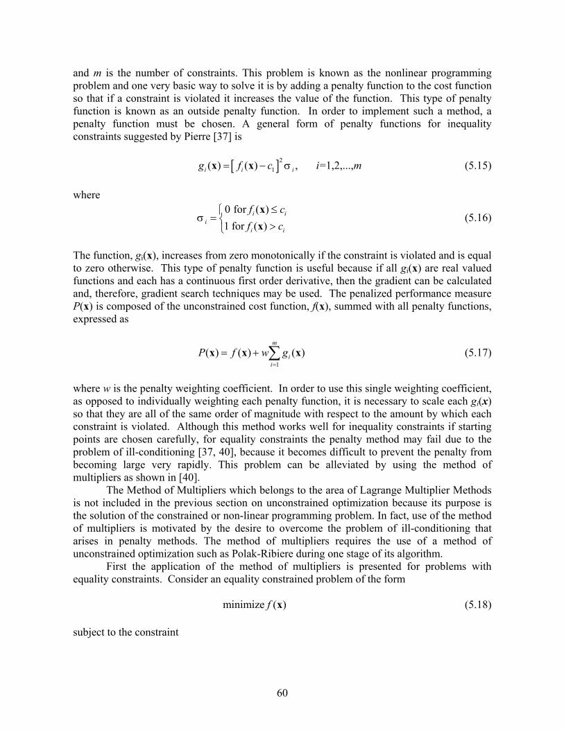
60
and m is the number of constraints. This problem is known as the nonlinear programming problem and one very basic way to solve it is by adding a penalty function to the cost function so that if a constraint is violated it increases the value of the function. This type of penalty function is known as an outside penalty function. In order to implement such a method, a penalty function must be chosen. A general form of penalty functions for inequality constraints suggested by Pierre [37] is
[ ]21( ) ( ) , =1,2,...,i i ig f c i mσ= −x x (5.15)
where
0 for ( )1 for ( )
i ii
i i
f cf c
σ≤
= >
xx
(5.16)
The function, gi(x), increases from zero monotonically if the constraint is violated and is equal to zero otherwise. This type of penalty function is useful because if all gi(x) are real valued functions and each has a continuous first order derivative, then the gradient can be calculated and, therefore, gradient search techniques may be used. The penalized performance measure P(x) is composed of the unconstrained cost function, f(x), summed with all penalty functions, expressed as
1( ) ( ) ( )
m
ii
P f w g=
= + ∑x x x (5.17)
where w is the penalty weighting coefficient. In order to use this single weighting coefficient, as opposed to individually weighting each penalty function, it is necessary to scale each gi(x) so that they are all of the same order of magnitude with respect to the amount by which each constraint is violated. Although this method works well for inequality constraints if starting points are chosen carefully, for equality constraints the penalty method may fail due to the problem of ill-conditioning [37, 40], because it becomes difficult to prevent the penalty from becoming large very rapidly. This problem can be alleviated by using the method of multipliers as shown in [40].
The Method of Multipliers which belongs to the area of Lagrange Multiplier Methods is not included in the previous section on unconstrained optimization because its purpose is the solution of the constrained or non-linear programming problem. In fact, use of the method of multipliers is motivated by the desire to overcome the problem of ill-conditioning that arises in penalty methods. The method of multipliers requires the use of a method of unconstrained optimization such as Polak-Ribiere during one stage of its algorithm.
First the application of the method of multipliers is presented for problems with equality constraints. Consider an equality constrained problem of the form
minimize ( )f x (5.18)
subject to the constraint

61
( ) 0h =x (5.19)
When using the ordinary Lagrange method with the Lagrange function
( , ) ( ) ( )F f hλ λ= +x x x (5.20) a point x* can be a constrained local minimizing point for f(x) and not be an unconstrained local minimizing point of the Lagrange function, F(x,λ). The method of multipliers solves this problem by the addition of penalty terms to F to form an augmented Lagrangian. Such a penalized Lagrange function has the property that it is minimized with respect to x at x* whenever x* is a constrained minimizing point of f(x). The augmented Lagrangian function is expressed as
21( , ) ( ) ( ) ( )2cL f h w hλ λ= + +x x x x (5.21)
where w, the penalty weight, is any scalar and λ is the Lagrange multiplier. In the method of multipliers, given a multiplier vector λk and a penalty weight wk, at each k iteration Lck(x,λk) is minimized using an unconstrained method of minimization to obtain a new vector xk. Then the multiplier is iterated as
1 ( )k k k kw hλ λ+ = + x (5.22) a penalty weight wk+1 ≥ wk is chosen and the process is repeated. It is proven by Bertsekas [40] that for the penalty method, where λk ≡ const, it is usually necessary to increase wk to infinity. However, for the method of multipliers it is not necessary to increase wk to infinity to obtain convergence. Therefore, it eliminates or at least moderates the problem of ill-conditioning. Also, the convergence rate is generally much better than that of the penalty method. Next consider the case when there is an inequality constrained problem of the form
minimize ( )f x (5.23)
subject to the constraints
( ) 0, 1, 2,...,ig i m≤ =x where m is the number of constraints. It is possible to convert this nonlinear programming problem into an equality constrained problem by introducing additional variables, sometimes referred to as slack variables, r = (r1, r2, … , rm). This gives the new problem

62
21 1
22 2
2
minimize ( )subject to ( ) 0 ( ) 0 ( ) 0m m
fg r
g r
g r
+ =
+ =
+ =
xxx
x
(5.24)
Then x* is a local minimum of (5.23) if and only if (x*,r*), where * *( ), 1,...,i ir g x i m= − = , is a local minimum of problem (5.24). By using this conversion we can extend the method of multipliers to the nonlinear programming problem. The augmented Lagrangian becomes
22 2
1
1( , , ) ( ) ( ) ( )2
m
c i i i i ii
L f g r w g rµ=
= + + + + ∑x r µ x x x (5.25)
for c > 0. The augmented Lagrangian must be minimized with respect to the variables x and r for various values of the multiplier µ, and the constraint weight w. Fortunately, it is shown by Bertsekas [40] that the minimization of Lc with respect to r can be carried out explicitly for each fixed x. Note that
22 2
1
1min ( , , ) ( ) min ( ) ( )2
m
c i i i i ir riL f g r w g rµ
=
= + + + + ∑x r µ x x x (5.26)
The minimization with respect to ri is equivalent to
[ ] 2
0
1min ( ) ( )2i
i i i i iug u w g uµ
≥
+ + +
x x (5.27)
Because it is quadratic in ui, its minimum is the scalar ûi at which point the derivative equals zero. This gives
[ ]ˆ( ) 0i i iu w g u+ + =x (5.28) There are two possible cases for û. Either ˆ 0iu ≥ and, therefore, ûi solves (5.27), or the solution is * 0iu = . Therefore, the solution of (5.27) can be expressed as
* max 0, ( )ii iu g
wµ = − +
x (5.29)
By (5.26)-(5.29) we obtain the following expression for the augmented Lagrangian for the nonlinear programming problem (5.23)

63
[ ] 2 2
1
1( , ) ( ) max(0, ( ))2
m
c i i ii
L f wgw
µ µ=
= + + −∑x µ x x (5.30)
Extending the results of the Lagrange multiplier method for equality constrained problems, the first order multiplier iteration is given by
[ ]1 max , ( , )i
i i kk k k i k k
k
w g wwµ
µ µ µ+
= + −
x (5.31)
which can be further simplified in the final form
[ ] 1 max 0, ( , )i ik k k i k kw g wµ µ µ+ = + x (5.32)
Given a multiplier vector µk and a penalty weight wk, at each iteration k Lck(x,µk) is minimized using an unconstrained method of minimization to obtain a new vector xk. Then the multiplier is iterated as µk+1 where 1
ikµ + is the ith element.
5.3 Optimization of Conventional RHFs
In order to reduce the harmful effects of minor harmonics on the effectiveness of conventional RHFs, a few strategies may be employed during filter design. Each filter branch compensates a portion of the load reactive power. How the reactive power is distributed among the branches determines the locations of the resonant frequencies. Therefore, resonant frequencies may be shifted by changing the allocation of reactive power to particular branches. This shifting can also be accomplished by over or under-compensation of the load reactive power. Also, if distribution voltage harmonics are present, de-tuning the filter branches will reduce the sensitivity of the filter to distribution voltage harmonics. A trial and error approach employing the above strategies may be used to adjust filter parameters in order to achieve better performance. However, as discussed in sections 3.2 and 3.3, it is unlikely that the best results will be achieved. In order to obtain the best possible performance in the presence of minor harmonics optimization methods should be used.
For conventional RHFs the cost function defined by equation (5.6) is a function of the capacitance and inductance of the filter branches, f(x) = f(L1,C1,. . . .,LK,CK). Another option is to express it as a function of the tuned frequency and the reactive power allocation of each branch, f(x) = f(z1,d1,. . . .,zK,dK). The choice is rather a matter of preference since both are a function of 2K parameters, where K is the number of filter branches. The level of compensation of the load reactive power must be held constant or allowed to be varied within a range of acceptable compensation levels. Therefore, the optimization problem becomes a nonlinear programming problem with equality and inequality constraints.
Initially, the penalty function approach was applied to solve the minimization problem with constraints placed on the total reactive power of the filter. This method was found to give good results in the case of the inequality constraint where some range of over and under-compensation was allowed. However, for the equality constrained case a minimum was not always reached depending on the starting point. It was found that the penalty function was

64
increasing too rapidly and efforts were made to adjust the weighting. However, the balance between preventing constraint breakthrough and the penalized performance measure becoming ill-conditioned was difficult to achieve. The adjustment of the weighting factor had to be determined on a case-by-case basis. Therefore, the penalized performance measure (5.17) was abandoned and the method of multipliers was implemented. To implement the method of multipliers an augmented Lagrangian was formed using the cost function (5.6) and the reactive power constraints. For the case of unity load reactive compensation the augmented Lagrangian is equal to
22 2
1
1 1( , , ) ( ) ( ) ( ) max 0, ( )2 2
K
c c i i ii
L f h w h wgw
λ λ µ µ=
= + + + + − ∑x µ x x x x (5.33)
The equality constraint h(x) is
21 1( ) 0f Lh B U Q= − =x (5.34)
where Bf1 is the filter susceptance at the fundamental frequency, which is a function of the variables x, and QL is the load reactive power. The inequality constraints require that the n filter circuit elements be positive values. However, it is not necessary to constrain each filter circuit element separately. Recall that the susceptance of each k filter branch is capacitive at the fundamental frequency and can be expressed as
11 2
11
kk
k
CB ω
ωζ
=
−
(5.35)
and the inductance is related to the capacitance as
21
1( )k
k k
LCζ ω
= (5.36)
where ζkω1 is the branch tuned frequency and is always postive. If the susceptance is negative then by (5.35) the branch capacitance is negative which in turn yields a negative value of the branch inductance by (5.36). Thus, for a filter with K branches, there are K inequality constraints, and they can be expressed as
1( ) 0i ig B= − ≤x (5.37)
For the case where there is a range of over or under-compensation of load reactive power no equality constraints are needed and the augmented Lagrangian becomes
2 2 2
1
1( , ) ( ) max 0, ( )2
K
c c i i ii
L f wgw
µ µ+
=
= + + − ∑x µ x x . (5.38)

65
The constraint g1(x) specifies the upper limit of the over-compensation and is equal to
21 1 1 1( ) 0f Lg B U c Q= − + ≤x (5.39)
where a multiplied by the reactive power of the load, QL, specifies the upper limit of the overcompensation. If the reactive power of the filter exceeds aQL then g1(x) will increase. The lower limit of under-compensation is specified by g2(x) and is equal to
22 1 1 2( ) 0f Lg B U c Q= − ≤x . (5.40)
where bQL specifies the lower limit. If the reactive power of the filter is lower than bQL, then g2(x) will increase. As previously the other K constraints are simply to ensure that filter circuit elements are positive, and they are also given by (5.37). The method of multipliers requires the adjustment of the penalty weighting factor, w, similarly as for the penalty method. The weighting factor was updated according to
1k kw wγ+ = (5.41) However, in this case there was no need to dynamically adjust the weighting as in the case of the penalty method. A constant value for the weight increase of γ=1.2 was used to obtain the results presented in subsequent chapters. The method converged to a constrained local minimum of fc(x) from any valid starting point. 5.4 Optimization of RHFs with Line Inductor The fixed-pole RHF allows much better control of the filter design process with respect to the selection of both branch tuned frequencies and the frequencies of the filter poles. In spite of this, it may not be obvious to the designer what the best choice of zeros and poles of the filter are. Although fixed-pole RHF will generally exhibit much better performance than a conventional RHF when operated in the presence of minor harmonics, it is unlikely that the best performance would be achieved without the use of optimization techniques as part of the design process. Because of this, it is difficult to expect that a trial and error approach may provide satisfactory results.
The term “fixed-pole” describes an attribute of the synthesis of such filters where the designer fixes the filter poles at some predetermined frequencies. If filter parameters are modified by an optimization routine then the term losses its meaning since the poles are no longer fixed at their predetermined locations. Thus, the term fixed-pole RHF will refer to the pre-optimized filter prototype and after optimization is performed the filter will simply be referred to as an optimized RHF with line inductor. The number of circuit elements of the RHF with line inductor is greater than the number of elements of a conventional RHF due to the added series inductor L0. Therefore, the cost function (5.6) should not be a function of the circuit elements since this would require 2K+1 parameters. Also, the number of constraints required would be greater than for the conventional RHF. If the filter zeros and poles are selected as the parameters then only 2K

66
parameters are needed since the series inductor, L0, is a function of those parameters. Therefore, the cost function is fc(x) = f(z1,p1, … ,zi,pi, … ,zK,pK) where zi is the series tuned frequency of the ith filter branch and pi is the frequency of the pole that results from the resonance between the ith branch and the series inductance Lx = Ls + L0. The constraints for the RHF with line inductor are also quite different from those of the conventional RHF. Since the reactive power provided by the filter is selected initially and is not affected by changing the zero and pole allocations of the filter, filter reactive power is no longer a constraint. However, as shown in section 4.3 there exists combinations of zero and pole allocations that result in a negative value of L0. Of course, this is not physically realizable. Also, there are some upper bounds on the value of L0 depending on the application. These limits depend on the allowable effect of L0 on the load voltage variation. The poles must be selected such that zi-1 < pi < zi, that is, for each branch the pole associated with it must have a lower frequency than that branch’s series tuned frequency or zero. However, the pole must have a greater frequency than the closest zero due to another branch that has a lower frequency or the fundamental, i.e. poles and zeros must alternate. If this condition is violated then the filter transfer function is not a positive real function and cannot be realized by a circuit having only elements with positive parameters, [51]. A negative circuit element would require that at least one branch have a negative susceptance at the fundamental frequency. A branch susceptance at the fundamental frequency equal to zero occurs if a pole and zero cancel and this yields a solution with a reduced number of branches. Therefore, direct constraints on the allocation of zero and pole frequencies are not needed since negative susceptance for any branch will not be allowed. This gives an inequality constrained problem of the form (5.23) where m is the number of constraints. The augmented Lagrangian is the same as for the conventional RHF given in (5.38) only the constraints and the variables x are different. Each constraint gi(x) for i=1,2,3,…,K is violated if the susceptance at the fundamental for a filter branch is less than zero. Therefore the first K constraints are equal to
1( ) 0i ig B= − <x . (5.42) There is also a constraint for each the lower and upper bound of L0 as it relates to the system inductance Ls, such that 1 0 2s sa L L a L≤ ≤ . For the lower limit of L0 the constraint is equal to
1 0 1( ) 0K sg L a L+ = − + ≤x , (5.43)
and for the upper limit the constraint is equal to
2 0 2( ) 0K sg L a L+ = − ≤x . (5.44)
This yields m=K+2 constraint equations for the filter. 5.5 The Global Minimum
The cost function fc(x) for both RHFs with line inductor and conventional RHFs has multiple local minima and maxima. When filter parameters are selected such that a resonant frequency approaches a harmonic frequency a sharp increase in the cost function value may
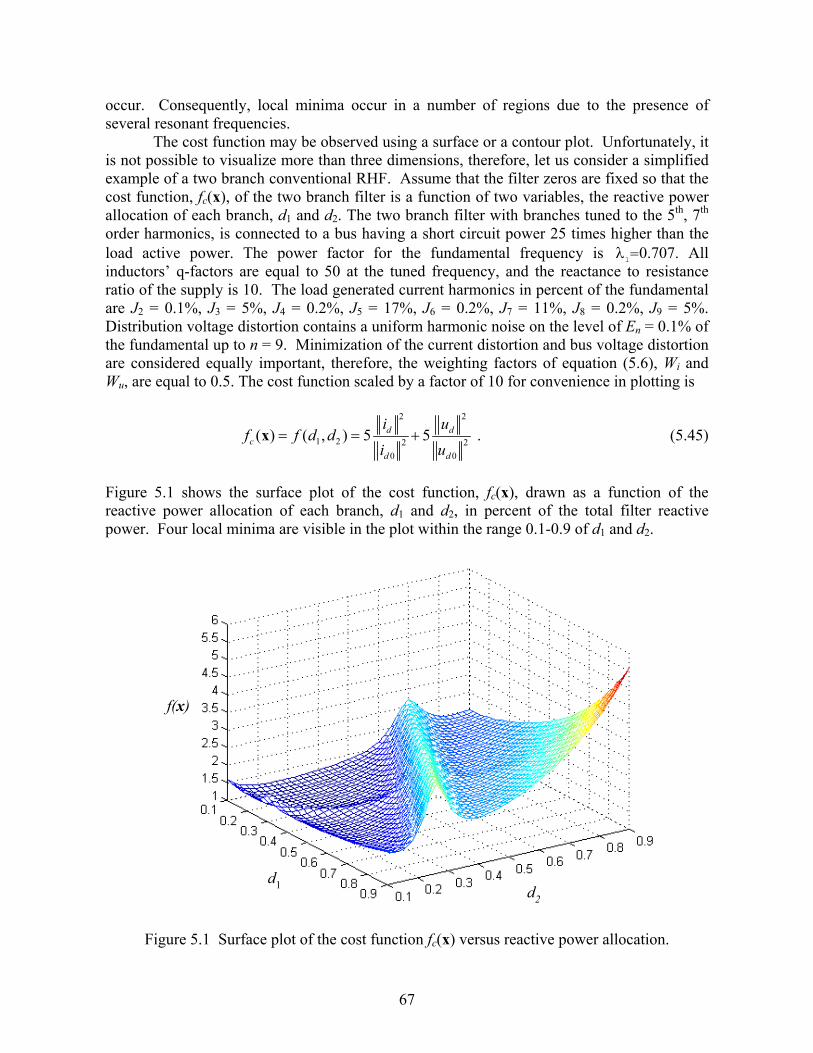
67
occur. Consequently, local minima occur in a number of regions due to the presence of several resonant frequencies.
The cost function may be observed using a surface or a contour plot. Unfortunately, it is not possible to visualize more than three dimensions, therefore, let us consider a simplified example of a two branch conventional RHF. Assume that the filter zeros are fixed so that the cost function, fc(x), of the two branch filter is a function of two variables, the reactive power allocation of each branch, d1 and d2. The two branch filter with branches tuned to the 5th, 7th order harmonics, is connected to a bus having a short circuit power 25 times higher than the load active power. The power factor for the fundamental frequency is λ1=0.707. All inductors’ q-factors are equal to 50 at the tuned frequency, and the reactance to resistance ratio of the supply is 10. The load generated current harmonics in percent of the fundamental are J2 = 0.1%, J3 = 5%, J4 = 0.2%, J5 = 17%, J6 = 0.2%, J7 = 11%, J8 = 0.2%, J9 = 5%. Distribution voltage distortion contains a uniform harmonic noise on the level of En = 0.1% of the fundamental up to n = 9. Minimization of the current distortion and bus voltage distortion are considered equally important, therefore, the weighting factors of equation (5.6), Wi and Wu, are equal to 0.5. The cost function scaled by a factor of 10 for convenience in plotting is
2 2
1 2 2 20 0
( ) ( , ) 5 5d dc
d d
i uf f d d
i u= = +x . (5.45)
Figure 5.1 shows the surface plot of the cost function, fc(x), drawn as a function of the reactive power allocation of each branch, d1 and d2, in percent of the total filter reactive power. Four local minima are visible in the plot within the range 0.1-0.9 of d1 and d2.
d1 d2
f(x)
Figure 5.1 Surface plot of the cost function fc(x) versus reactive power allocation.

68
A contour plot of the cost function is shown in Figure 5.2. The plot shows the multiple local minima that are separated by the ridges formed when the resonant frequencies and harmonic frequencies coincide. The ridge that runs down the center of the plot is formed at the values of d1 and d2 for which a resonance is located at the 4th order harmonic as shown in Fig. 5.3 (a).
0.1 0.2 0.3 0.4 0.5 0.6 0.7 0.8 0.90.1
0.2
0.3
0.4
0.5
0.6
0.7
0.8
0.9
1.1807
1.2239
1.2671.3101
1.3532
1.267
1.3101
1.3532 1.3963 1.4394
1.9567 2.0429
1.9998
2.086
2.21542.1723
2.2585
2.3016
2.34472.5171
2.9482 3.3362
4.026
1.5687
1.6118 1.8705
1.8274
d1
d2
Figure 5.2 Contour plot of the cost function fc(x).
Figure 5.3 (b) shows the resonant frequency locations for values of d1 and d2 that correspond to a local minimum of fc(x). At this local minimum the resonant frequencies are much further from harmonic frequencies.
Figure 5.3 Resonant bands of amplification for values of d1 and d2 on a ridge (a) and near a
minimum (b) of fc(x).

69
Although there are four local minima for the cost function, fc(x), this function is
unconstrained. If full load reactive power compensation is required and the reactive power allocated to a particular branch cannot be lower than 10% of the filter reactive power, then the constrained problem is
1 1 2
2 1
3 2
minimize ( )subject to ( ) 1 0 ( ) 0.1 0 ( ) 0.1 0
cfg d dg dg d
= + − == − ≥= − ≥
xxxx
(5.46)
The constrained cost function will yield a minimum which is confined to the dotted line shown on the contour plot in Figure 5.4, and the boundary of the plot shown is specified by all three constraints. The line indicates that the sum of the reactive power allocation of all branches must equal one. In this case the minimum would be chosen from the best of those local minima that the constraint line intersects.
0.1 0.2 0.3 0.4 0.5 0.6 0.7 0.8 0.90.1
0.2
0.3
0.4
0.5
0.6
0.7
0.8
0.9
1.1807
1.2239
1.2671.3101
1.3532
1.267
1.3101
1.3532 1.3963 1.4394
1.9567 2.0429
1.9998
2.086
2.2154
2.1723
2.2585
2.3016
2.34472.5171
2.9482 3.3362
4.026
1.5687
1.6118 1.8705
1.8274
d1
d2
Figure 5.4 Contour plot of cost function fc(x) and the constraint g1(x).
The presence of multiple minima indicates that a method of global optimization is
needed. Since the mechanism that causes multiple local minima in the case of this cost function is known, it is possible to use the optimization techniques described above. These can be employed by repeated use of the routines at starting points near each local minimum. The local minima can then be compared and the global minimum identified. The RHF with line inductor has a distinct advantage over the conventional RHF when employing such a global minimization strategy. This is because the frequencies of the filter poles can be
70
selected directly as parameters of the optimization. Therefore, the starting points of the poles can be selected so that each filter pole is located initially between as many harmonic frequencies as possible, giving a clear set of starting points bounded by points that give higher values of the constrained cost function. In the case of conventional RHFs it is not known a-priori where the poles of the filter will be located when starting values of the reactive power allocation are chosen. Therefore, it is only possible to select a large enough random set of starting points such that there is a high probability of finding the global minimum. Needless to say, that approach is not efficient. It should be mentioned that although a particular local minimum may be the best with respect to the cost function value, it may not be acceptable from the viewpoint of sensitivity. A matrix sensitivity measure could be developed based on the behavior of the Hessian matrix for the region around the optimal point. The development of such a measure for optimized RHFs that would enable the determination of the component tolerances necessary to maintain sufficient filter effectiveness could be an area of future research. 5.6 Specialized Optimization Software
Due to the complexity of the interaction between a RHF and system, optimization cannot be done analytically. Therefore, in order to perform the optimization described in the previous sections, a software program for performing optimized design of RHFs is needed. The program must perform the analysis and optimization of conventional RHFs and RHFs with a line inductor. Therefore a specialized program for those tasks was developed in the C++ programming language. Although software packages for general optimization and analysis, such as Matlab, already exist, the use of C++ allows a much higher level of customization. A high degree of customization is desirable with respect to the optimization algorithms as well as a graphical user interface which is tailored to filter design.
The user interface of the developed program is entirely based on drop down menus and dialog boxes, and there are multiple view modes for viewing the circuit model, transmittance plots, distortion coefficients, etc. The settings for the distribution system, load, filter, and harmonic spectra may be changed while in any of the view modes. This allows the user to see the effects on the circuit element values, the performance coefficients and on the frequency properties as the user input parameters are varied. Thus, the various views provide a powerful tool for a filter designer to determine the effects of changes in the system and filter as well as the harmonic spectra. The view and plots are useful features of the software in addition to it providing the optimized parameters of a filter. A brief description of the user interface and instructions for use are included in the appendix.
The program performs four primary tasks. First, it allows the user to specify system parameters and input the distribution voltage and load generated current harmonic spectra up to the 30th harmonic order. From this data the program calculates the parameters of a prototype filter. The user selects the tuned frequencies, reactive power allocation or poles depending on the filter type, load compensation level, q-factor, and number of branches the filter has. The second task of the program is to provide performance analysis of this filter prototype. It calculates and displays all of the filter’s performance measures with respect to the voltage and current distortion and the levels of the contributing components of the distortion. Next, the RHF is optimized using the method of multipliers. Finally, the resulting filter is analyzed with respect to its performance, and the performance data is displayed.

71
Chapter 6
Effectiveness of Resonant Harmonic Filters in a System with a AC/DC Converter
6.1 Introduction
One of the most common applications of RHFs is the reduction of harmonic distortion produced by six-pulse AC/DC controlled converters or rectifiers. Therefore, a system that supplies a six-pulse converter is used as the test system for evaluating filter performance in this chapter.
Although optimization techniques allow the design of filters with the highest effectiveness, at some level of minor harmonics even optimized filters are not sufficiently effective. In order to evaluate the performance of conventional RHFs designed according to references [1, 4, 11, 12, 15, 19, 20] as compared to those optimized using the techniques described in chapter 5, simulation results for some typical voltage and current spectra are presented in this chapter. Also, simulation results for an optimized RHF with line inductor are given and compared to the optimized conventional RHF. To evaluate filter performance at different levels of minor harmonics content, the level of minor harmonics is increased in intervals and optimized filter effectiveness is found for each of them. In order to evaluate the limits of filter effectiveness for the conventional and RHFs with line inductor, IEEE Std 519-1992, [35], is used as the basis for determining when effectiveness is not sufficient. 6.2 The Test System Harmonic filters are used under various operating conditions with a wide variety of loads and harmonic spectra. Of course, it is not possible to check the performance of RHFs that are designed using the techniques presented in chapter 5 for all of the various operating conditions that such filters are used in. Therefore, a typical system and load are used as the basis for filter performance evaluation. A distribution system that supplies a six-pulse AC/DC controlled converter with the following parameters is used as such a test system. The six-pulse controlled converter is supplied from a 60 Hz symmetrical three-phase distribution system with a short circuit power of 21.2 pu and with a reactance to resistance ratio at the fundamental frequency, Xs/Rs equal to 10. The distorted component of the load generated current, j, is composed of the characteristic harmonics of a six pulse converter with the RMS value J5 = 18%, J7 = 13%, J11 = 8%, and J13 = 7% of the fundamental. The load current also contains minor harmonics caused by the thyristor firing control asymmetry. The distribution of the minor harmonics in the load current is random, it varies from converter to converter and also with changes in the firing angle. It is assumed for this test system that the minor harmonics in the current have a uniform value up to the 12th order harmonic. This assumption is further justified by [16] which provides the current spectrum of a typical converter and shows minor harmonics which are of approximately the same magnitude. Harmonics above the 13th order are neglected since they cannot be amplified by filter resonances. Various levels of minor harmonics are considered. However, initially it is assumed that minor harmonics comprise a distorted component of the load current, denoted as δjm, equal to 1.5% of the fundamental. This means that the minor current harmonics

72
generated by the converter are of the value Jn=0.53% of the fundamental. The spectrum of the load current is shown in Fig. 6.1.
Load Current Spectrum
0%
2%
4%
6%
8%
10%
12%
14%
16%
18%
20%
2 3 4 5 6 7 8 9 10 11 12 13Harmonic Order
Perc
ent o
f Fun
dam
enta
l
Figure 6.1 Harmonic spectrum of the load generated current, j, for δjm=1.5%.
The IEEE recommended limit for the distortion of the distribution voltage e, given in
Table 2.2, is δe = 5% of the fundamental. Therefore, various levels of voltage distortion up to δe= 5% are used to evaluate filters for the range of allowed voltage distortion. The magnitude of the voltage harmonics are assumed to decline as 1/n and the even order harmonics have a magnitude which is 25% of the odd order harmonics. For the initial system evaluation let us assume that the utility provides a voltage with the level of distortion at half of the recommended limit, δe = 2.5% of the fundamental. Then the distribution voltage harmonics up to the 13th order are equal to
1
1
15.31 , for even415.31 , for odd.
n
n
E E nn
E E nn
= =
= = (6.1)
The harmonic spectrum of the distribution voltage, e, is shown in Fig. 6.2.
Six-pulse AC/DC converters allow the control of the DC output voltage by variation of the thyristor firing angle, α. The output voltage, Ud0, of the converter shown in Fig. 2.2 as a function of firing angle is
03 6 cosdU U απ
= (6.2)

73
where U is rms value of the bus voltage supplying the converter. Therefore both active power and reactive power of the converter will change with the firing angle.
Distribution Voltage Spectrum
0.0
0.2
0.4
0.6
0.8
1.0
1.2
1.4
1.6
1.8
2.0
2 3 4 5 6 7 8 9 10 11 12 13Harmonic Order
Perc
ent o
f Fun
dam
enta
l
Figure 6.2 Harmonic spectrum of the distribution voltage, e, for δe=2.5%.
Because the change in the firing angle changes the phase-shift between voltage and current, the active and reactive power, expressed as a function of firing angle, α, are equal to
2max
max
cos ( )1 sin(2 )2
P P
Q P
α
α
=
= (6.3)
A plot of the normalized active power, i.e. for Pmax=1, and reactive power versus firing angle is shown in Fig. 6.3.
Figure 6.3 Active and reactive power versus firing angle.

74
In order to simplify the comparison of the harmonic filters in this chapter, load parameter variation is not considered. Therefore, the converter is assumed to operate at a constant firing angle α=45° with a normalized apparent power, SL, equal to 1 pu, i.e., both active power, P, and reactive power, Q, of the load are equal to 0.71 pu. The single-phase equivalent circuit for the test system is shown in Fig. 6.4. The waveforms of the distribution voltage, e, the bus voltage, u, and the supply current, is, are shown in Fig. 6.5. The supply current has the distortion δi = 23.7% of the fundamental, and at such current distortion the bus voltage has the distortion δu = 7.9% of the fundamental.
RL= 0.707
LS=124 H
e
Distribution System
RS=4.7m
uis
j
Load
LL=124 mH
µΩ
Ω
Figure 6.4 Single-phase equivalent circuit of the test system without filter.
Figure 6.5 Voltage and current waveforms of the test system without filter.
With the converter operating at α = 45° the system short circuit current to load current ratio, ISC/IL, is equal to 30. For such a ratio the IEEE Std. 519 recommended limit, as shown in Table 2.1, for individual odd harmonics in the current is 7% up to the 10th order and 3.5% for the

75
11th, 12th and 13th order harmonics. The total distortion of the current is limited to 8% of the fundamental. Thus, all of the characteristic harmonics exceed their recommended limits as well as exceed the limit for the total harmonic distortion of the supply current. All minor harmonics are within the specified limits. Clearly a device for suppression of characteristic current harmonics is needed. Recall that the total harmonic distortion of the supply current, δi, is the ratio of the rms values of the distorted component of the current and the fundamental. Since the fundamental current of the supply depends on the power factor, it can be expressed as
1
di
a
iI
λδ = (6.4)
where Ia1 is the rms value of the active current at the fundamental. Therefore, the harmonic distortion after the installation of a filter not only depends on the filter’s ability to reduce the rms value of the distorted component of the current, but also, the load reactive power compensation provided by the filter. To determine a filter’s true effectiveness in the reduction of the distorted component rms value, the effectiveness in reduction of current distortion, εi, defined by equation (5.1) should be used. This means that the minimum effectiveness of a filter required to meet the IEEE Std. 519 limits for current distortion depends on how the filter affects the power factor. Let λf denote the power factor after the installation of a filter. Then the minimum allowable filter effectiveness in reduction of current distortion, εi min, can be expressed as
maxmin
0
(1 ) 100ii
f i
λδε
λ δ= − × (6.5)
where δi max is the allowed limit for the total current distortion and δi0 is the initial current distortion in percent of the fundamental without the filter. In this equation power factor, λ, is assumed to be power factor prior to filter installation. Assuming the filter is required to fully compensate the load reactive power, to achieve the 8% total harmonic distortion limit the effectiveness of the filter for the test system cannot be lower than εi min = 76.1%. 6.3 Conventional RHF Performance
Conventional RHFs for filtering harmonics generated by six-pulse converters usually have four branches, each tuned to a characteristic current harmonic generated by the converter. Therefore, a four branch RHF tuned to the 5th, 7th, 11th, and 13th order harmonics is considered as the starting point for the optimized conventional RHF. As discussed in section 3.2, such filters are usually slightly detuned from harmonic frequencies or damped to limit currents due to distribution voltage harmonics on the supply side of the filter. However, opinion regarding the allocation of reactive power among the branches varies widely. The various strategies can be divided roughly into two groups: some predefined criteria for the allocation, [1, 19, 20], and trial and error adjustment based on simulation results and designer experience, [4, 11, 12, 15]. Therefore, three different sets of conventional RHFs are evaluated. The first two sets of filters were designed using strategies that belong to the above mentioned groups and the third was designed using the optimization method described in section 5.3. They were designed assuming

76
that these filters fully compensate the reactive power of the load and all inductors have a q-factor equal to 50 at their branch’s tuned frequency. 6.3.1 Conventional RHFs with Equal Allocation of Branch Reactive Power
The first filter set, designated RHF-1, is designed according to Ref. [1]. The load reactive power compensation is shared equally by the four branches and they are tuned to the 5th, 7th, 11th, and 13th order harmonics. Filter parameters are given in Table 6.1. Because the filter parameters are independent of the distribution voltage spectra, only one filter is designed for this set.
Table 6.1 Filter parameters
Branch 1 2 3 4 L [mH] 0.625 0.313 0.125 0.089 C [mF] 0.450 0.459 0.465 0.466 ωn/ω1 5.00 7.00 11.00 13.00
dk 0.25 0.25 0.25 0.25 The magnitude of the A(jω) and B(jω) transmittances for the filter and test system are
shown in Fig. 6.6 (a), and the magnitude of the admittance Y(jω) is shown in Fig. 6.6 (b). The values of all transmittances at harmonic frequencies are compiled in Table 6.2.
Figure 6.6 Magnitude of A(jω), B(jω) and Yx(jω) transmittances for RHF-1.
While the filter substantially reduces the characteristic current harmonics generated by
the load, the high values of admittance at several harmonic frequencies result in an increase in supply current distortion due to distribution voltage harmonics. Also, there is a contribution due to values of An and Bn transmittances which are above one indicating amplification due to resonance. The values of harmonic transmittance, Zyn, are much less than one for nearly all harmonics. Therefore, the impedance for the load generated harmonics does not cause reduction of the filter effectiveness. The values of the filter’s effectiveness measures, εi and εu, as well as the distortion coefficients, δi and δu, for distribution voltage distortion equal to δe=0.5%, δe=2.5%, and δe=5% are compiled in Table 6.3 for the load current spectrum shown in Fig. 6.1.

77
Table 6.2 Filter transmittances at harmonic frequencies
for RHF-1. n An & Bn Yxn Zyn 2 1.09 1.07 0.10 3 1.42 3.04 0.20 4 4.40 18.34 0.82 5 0.09 4.27 0.02 6 4.29 18.14 1.20 7 0.05 3.04 0.01 8 0.88 0.52 0.33 9 1.04 4.82 0.44 10 0.21 2.58 0.10 11 0.02 1.93 0.01 12 0.57 1.96 0.32 13 0.01 1.63 0.01
Table 6.3 Filter Effectiveness at different values of distribution voltage distortion for RHF-1.
δe in percent of the Fund.
εi %
εu %
δi %
δu %
0.5 81.5 85.2 6.4 1.2 2.5 52.8 57.5 16.4 3.3 5.0 9.9 17.6 31.4 6.5
The effectiveness of the filter is drastically reduced with increasing values of δe, and it is
much lower than the minimum required effectiveness, εi min= 76.1%, at δe=2.5%. The effect of δe on the waveform and harmonic spectrum of the supply current for δe=2.5% is shown in Fig. 6.7 and Fig. 6.8 respectively.
Figure 6.7 Supply and load current waveforms in the test system with RHF-1 and δe=2.5%.

78
Supply and Load Current Spectrum
0.000
0.020
0.040
0.060
0.080
0.100
0.120
0.140
0.160
0.180
0.200
2 3 4 5 6 7 8 9 10 11 12 13Harmonic Order
Cur
rent
(per
uni
t)
Load Current Supply Current
Figure 6.8 Harmonic spectrum of the load and supply current for the test system
with RHF-1 and δe=2.5%. 6.3.2 Optimized Conventional RHFs with Limited Detuning
The second filter set, designated RHF-2, represents the group of filters designed using a trial and error approach which is based on simulation. Unfortunately, results of such a strategy would vary according to the experience and design philosophies of the filter designer. Therefore, optimization with additional restrictions could be performed to simulate the best case design using the trial and error approach. Literature which promotes this approach only suggests a slight de-tuning of the filter branches from the characteristic harmonic frequencies of the load current while all adjustments are performed on the branch reactive power allocation. Therefore, the set RHF-2 is designed by applying optimization techniques with the additional restriction that the filter’s tuning frequencies may be only slightly de-tuned. Filter parameters for the set RHF-2 are given in Table 6.4.
Table 6.4 Filter parameters for set RHF-2 δe Branch 1 2 3 4
L [mH] 0.798 0.252 0.085 0.204 C [mF] 0.353 0.570 0.710 0.207 ωn/ω1 5.0 7.0 10.8 12.9
0.5%
dk 0.196 0.310 0.382 0.111 L [mH] 1.141 0.285 0.083 0.115 C [mF] 0.247 0.503 0.729 0.369 ωn/ω1 5.0 7.0 10.9 13
2.5%
dk 0.137 0.274 0.392 0.198 L [mH] 1.190 0.294 0.161 0.057 C [mF] 0.246 0.503 0.368 0.731 ωn/ω1 4.9 6.9 10.9 13
5.0%
dk 0.14 0.27 0.20 0.39

79
The magnitude of the A(jω), B(jω), and Y(jω) transmittances for the filter set and test system are shown in Fig. 6.9 (a) and (b) - Fig. 6.11 (a) and (b). The values of the filter’s effectiveness, εi and εu, as well as the distortion coefficients, δi and δu, for distribution voltage distortion equal to δe=0.5%, δe=2.5%, and δe=5% are compiled in Table 6.5 for the load current spectrum shown in Fig. 6.1.
Figure 6.9 Magnitude of A(jω), B(jω), and Yx(jω) transmittances for RHF-2 optimized for δe=0.5%.
Figure 6.10 Magnitude of A(jω), B(jω), and Yx(jω) transmittances for RHF-2 optimized for δe=2.5%.
Selecting the allocation of branch reactive power in order to move resonant frequencies
away from harmonic frequencies, yields improved performance with respect to filter RHF-1. Despite this, bands of high admittance with the resonant frequencies located away from
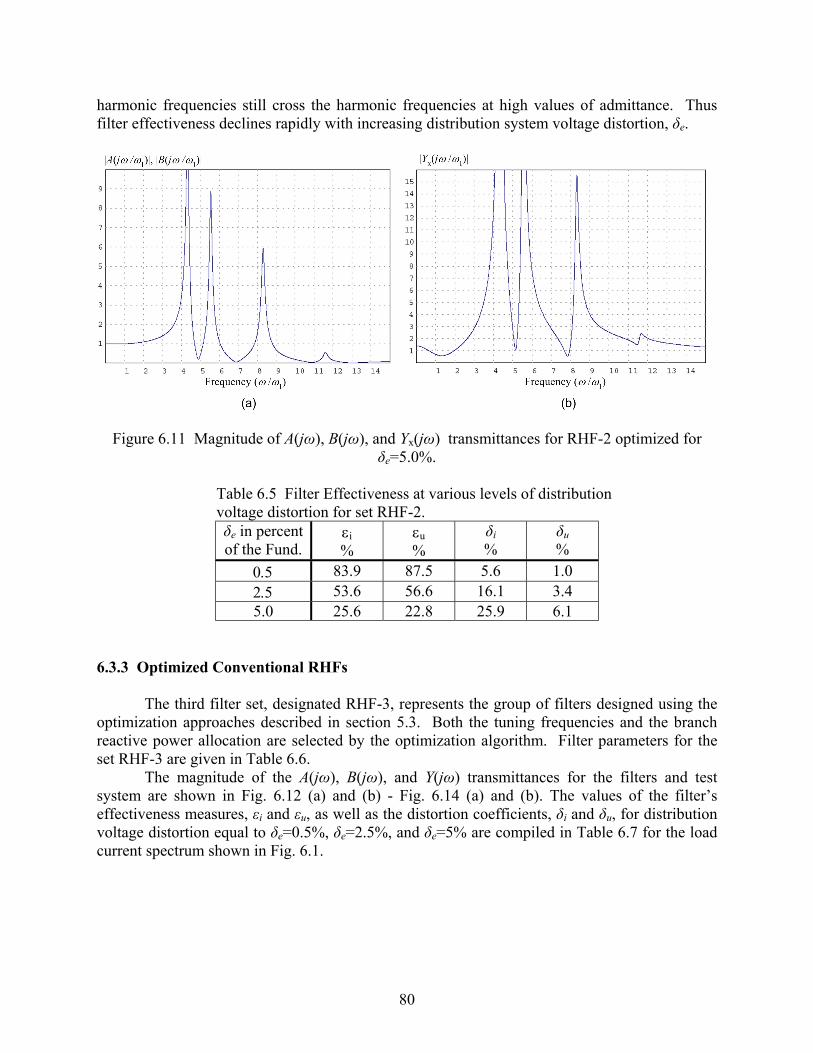
80
harmonic frequencies still cross the harmonic frequencies at high values of admittance. Thus filter effectiveness declines rapidly with increasing distribution system voltage distortion, δe.
Figure 6.11 Magnitude of A(jω), B(jω), and Yx(jω) transmittances for RHF-2 optimized for δe=5.0%.
Table 6.5 Filter Effectiveness at various levels of distribution voltage distortion for set RHF-2.
δe in percent of the Fund.
εi %
εu %
δi %
δu %
0.5 83.9 87.5 5.6 1.0 2.5 53.6 56.6 16.1 3.4 5.0 25.6 22.8 25.9 6.1
6.3.3 Optimized Conventional RHFs
The third filter set, designated RHF-3, represents the group of filters designed using the optimization approaches described in section 5.3. Both the tuning frequencies and the branch reactive power allocation are selected by the optimization algorithm. Filter parameters for the set RHF-3 are given in Table 6.6.
The magnitude of the A(jω), B(jω), and Y(jω) transmittances for the filters and test system are shown in Fig. 6.12 (a) and (b) - Fig. 6.14 (a) and (b). The values of the filter’s effectiveness measures, εi and εu, as well as the distortion coefficients, δi and δu, for distribution voltage distortion equal to δe=0.5%, δe=2.5%, and δe=5% are compiled in Table 6.7 for the load current spectrum shown in Fig. 6.1.

81
Figure 6.12 Magnitude of A(jω), B(jω), and Yx(jω) transmittances for RHF-3 optimized for δe=0.5%.
Figure 6.13 Magnitude of A(jω), B(jω), and Yx(jω) transmittances for RHF-3 optimized for δe=2.5%.
The optimization algorithm selects parameters for a filter that is not tuned to the
dominant harmonics in the load current. Instead the branch tuned to the 13th order harmonic is removed and a branch tuned slightly below the 3rd harmonic is added. Although this slightly reduces the ability of the filter to attenuate the 13th order load generated current harmonic, it significantly reduces the admittance at harmonic frequencies, Yxn, for the lower order distribution voltage harmonics. Also, other branches are de-tuned slightly as voltage distortion, δe, increases.

82
Figure 6.14 Magnitude of A(jω), B(jω), and Yx(jω) transmittances for RHF-3 optimized for δe=5.0%.
Table 6.6 Filter parameters for set RHF-3
δe Branch 1 2 3 4 L [mH] 2.675 0.443 0.345 0.130 C [mF] 0.317 0.635 0.415 0.426 ωn/ω1 2.8 5 7 11.3
0.5%
dk 0.19 0.35 0.23 0.23 L [mH] 1.797 0.557 0.404 0.175 C [mF] 0.537 0.527 0.365 0.326 ωn/ω1 2.7 4.9 6.9 11.1
2.5%
dk 0.33 0.30 0.20 0.17 L [mH] 1.465 0.632 0.435 0.225 C [mF] 0.684 0.457 0.333 0.260 ωn/ω1 2.6 4.9 6.9 10.9
5.0%
dk 0.42 0.25 0.18 0.14 Table 6.7 Filter Effectiveness at various levels of distribution voltage distortion for set RHF-3.
δe in percent of the Fund.
εi %
εu %
δi %
δu %
0.5 85.9 85.2 4.9 1.2 2.5 71.4 68.6 9.9 2.5 5.0 51.7 48.8 16.7 4.1

83
6.4 Performance of RHFs with Line Inductor
As shown in the previous section, even optimized conventional RHFs cannot achieve a sufficient effectiveness at half of the maximum distribution system distortion allowed in the IEEE 519 standard. The RHF with line inductor offers a reduced filter sensitivity to distribution voltage harmonics at the cost of voltage drop on the line inductor of the filter. A set of RHFs with line inductor is applied to the test system under the same conditions as for the conventional RHFs in the previous section. The optimization techniques described in section 5.4 are used to determine the best selection of pole and zero locations of the filter for each distribution voltage spectrum. However, the constraints for the value of the line inductor, L0, must be determined based on the allowable voltage drop across L0. 6.4.1 Optimized RHFs with Line Inductor
Optimized RHFs with line inductor are designed for the test system and both the filter zeros and poles are selected by the optimization algorithm. The inductance of the line inductor is constrained to be not higher than twice the distribution system inductance. Filter parameters for a set of Fixed-Pole RHFs optimized for δe=0.5%, δe=2.5%, and δe=5.0% with δjm=1.5% are given in Table 6.8.
Table 6.8 Filter parameters for the set of RHFs with line inductor.
δe Branch 1 2 3 4 L0 L [mH] 6.293 0.528 0.299 0.081 0.248 C [mF] 0.128 0.533 0.481 0.299 ωn/ω1 3 5 7 11.4
0.5%
pk 2.7 3.3 5.7 8.5 L [mH] 3.583 0.555 0.318 0.090 0.248 C [mF] 0.234 0.507 0.454 0.613 ωn/ω1 2.9 5 6.9 11.3
2.5%
pk 2.6 3.5 5.7 8.6 L [mH] 2.523 0.381 0.685 0.107 0.248 C [mF] 0.334 0.740 0.210 0.508 ωn/ω1 2.9 5 7 11.4
5.0%
pk 2.5 3.4 6.3 8.6 The optimal parameters for the filter do not vary much with increasing distortion in the
distribution voltage. Therefore, the magnitude of the A(jω), B(jω), Yx(jω), and Zy(jω) transmittances for the filter and test system are only shown for δe=2.5% in Fig. 6.15 (a) and (b), and Fig. 6.16 (a) and (b) respectively. The values of the filter’s effectiveness measures, εi and εu, as well as the distortion coefficients, δi and δu, for distribution voltage distortion equal to δe=0.5%, δe=2.5%, and δe=5% are compiled in Table 6.9 for the load current spectrum shown in Fig. 6.1.
The optimization results in a filter which is not tuned to the dominant harmonics in the load current as also in the case of filter set RHF-3. However, the fixed pole filter has much more freedom in selecting poles locations. In fact, only the constraint on the line inductance restricts

84
the selection. The optimized performance and distortion coefficients for the Fixed-pole RHFs are compiled in Table 6.9.
Figure 6.15 Magnitude of A(jω) and B(jω) for the RHF with line inductor optimized for
δe=2.5%.
Figure 6.16 Magnitude of Yx(jω) and Zy(jω) for the RHF with line inductor optimized for
δe=2.5%. Table 6.9 Filter Effectiveness at various levels of distribution voltage distortion for the set of RHFs with line inductor.
δe in percent of the Fund.
εi %
εu %
δi %
δu %
0.5 93.5 93.5 2.2 0.5 2.5 84.9 74.5 5.3 2.0 5.0 71.9 49.6 9.7 3.9

85
6.5 Comparison of Filter Performance
The results of the simulations of the various RHFs presented in previous section showed that the optimized conventional RHF and RHF with line inductor are much more effective in the reduction of waveform distortion than other RHFs at increased levels of the distribution voltage distortion. The effectiveness in reduction of supply current distortion, εi, of each filter is shown in Figure 6.17 for convience of comparison. The bar graph shows that for very low levels of distribution voltage distortion the optimized filters do not give a big advantage. Even the RHF designed without regard for resonant frequencies performs adequately with respect to the IEEE Std. 519 recommendations. This is not surprising since such filters were used very effectively in the past when they were installed in systems with very low distribution voltage distortion. However, when distribution voltage distortion approaches the limit of 5%, filters which are not optimized exhibit effectiveness which is far below acceptable levels.
Comparison of Filters' Effectiveness
0
10
20
30
40
50
60
70
80
90
100
0.5 2.5 5
δ e (%)
ε i (%)
RHF-1
RHF-2
RHF-3
RHFwLI
Figure 6.17 Comparison of effectiveness εi for the various RHFs.
6.6 Limits of Effectiveness
Comparison of the filter performance demonstrates that optimized RHFs that may be de-tuned perform much better than RHFs designed according to other techniques. It also demonstrates the dramatic increase in effectiveness of the RHF with line inductor over the conventional RHF in the presence of distribution system distortion. However, the preceding sections only check filter performance for a few values of the distribution system voltage distortion and a single value of the load generated minor harmonics. In order to determine the effectiveness of both the optimized conventional and RHF with line inductor, minor harmonics in the test system are increased in increments of 0.25%. Harmonic distortion of the distribution voltage is increased from δe=0.5% to δe=4% of the fundamental. Distortion of the load current due to minor harmonics is increased from δjm=0.5% to δjm=3% of the fundamental. For each value of the distortions δe and δjm, the parameters for an optimized RHF with line inductor and optimized conventional RHF are found and the effectiveness in reduction of supply current distortion, εi, is calculated. Each of the values of εi versus minor harmonic distortion for the filter with line inductor forms the surface shown in Fig. 6.18. This surface plot shows that the RHF with line inductor reaches the lowest allowable limit of 76.1% for εi at δjm=3% and δe=4%. Also
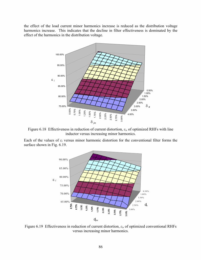
86
the effect of the load current minor harmonics increase is reduced as the distribution voltage harmonics increase. This indicates that the decline in filter effectiveness is dominated by the effect of the harmonics in the distribution voltage.
0.50
%
0.75
%
1.00
%
1.25
%
1.50
%
1.75
%
2.00
%
2.25
%
2.50
%
2.75
%
3.00
%
0.50%1.00%
1.50%2.00%
2.50%3.00%
3.50%
4.00%
75.00%
80.00%
85.00%
90.00%
95.00%
100.00%
ε i
δ jm
δ e
Figure 6.18 Effectiveness in reduction of current distortion, εi, of optimized RHFs with line
inductor versus increasing minor harmonics.
Each of the values of εi versus minor harmonic distortion for the conventional filter forms the surface shown in Fig. 6.19.
0 .5 0%1.0 0%
1.5 0%
2.0 0%
2.5 0%
3.0 0%
65.00%
70.00%
75.00%
80.00%
85.00%
90.00%
ε i
djm
de
Figure 6.19 Effectiveness in reduction of current distortion, εi, of optimized conventional RHFs
versus increasing minor harmonics.

87
The surface plot shows that the conventional RHF reaches the lowest allowable limit of 76.1% for εi at δjm=3% and δe=1.75%. The surface has a very similar shape as for the optimized RHFs with line inductor but the limit of effectiveness is crossed at a much lower voltage distortion.
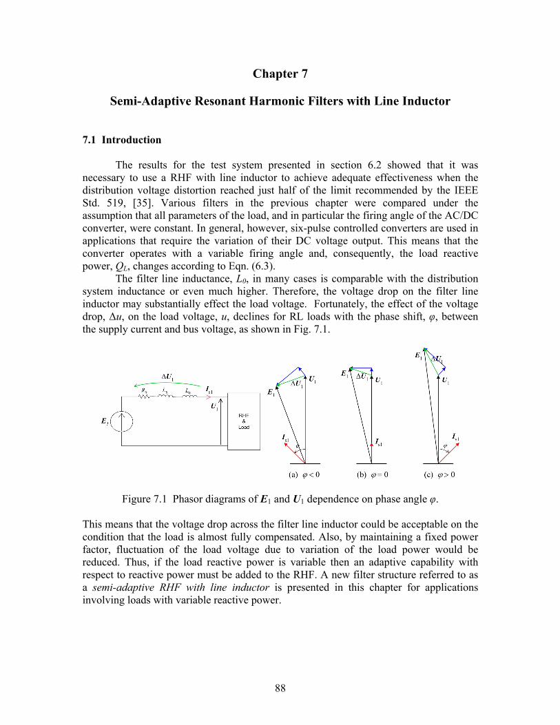
88
Chapter 7
Semi-Adaptive Resonant Harmonic Filters with Line Inductor 7.1 Introduction The results for the test system presented in section 6.2 showed that it was necessary to use a RHF with line inductor to achieve adequate effectiveness when the distribution voltage distortion reached just half of the limit recommended by the IEEE Std. 519, [35]. Various filters in the previous chapter were compared under the assumption that all parameters of the load, and in particular the firing angle of the AC/DC converter, were constant. In general, however, six-pulse controlled converters are used in applications that require the variation of their DC voltage output. This means that the converter operates with a variable firing angle and, consequently, the load reactive power, QL, changes according to Eqn. (6.3).
The filter line inductance, L0, in many cases is comparable with the distribution system inductance or even much higher. Therefore, the voltage drop on the filter line inductor may substantially effect the load voltage. Fortunately, the effect of the voltage drop, ∆u, on the load voltage, u, declines for RL loads with the phase shift, φ, between the supply current and bus voltage, as shown in Fig. 7.1.
Figure 7.1 Phasor diagrams of E1 and U1 dependence on phase angle φ. This means that the voltage drop across the filter line inductor could be acceptable on the condition that the load is almost fully compensated. Also, by maintaining a fixed power factor, fluctuation of the load voltage due to variation of the load power would be reduced. Thus, if the load reactive power is variable then an adaptive capability with respect to reactive power must be added to the RHF. A new filter structure referred to as a semi-adaptive RHF with line inductor is presented in this chapter for applications involving loads with variable reactive power.

89
7.2 Thyristor Switched Inductors
A device that provides variable susceptance is needed when full compensation must be maintained for loads with variable reactive power. A Thyristor Switched Inductor (TSI) is one such device which provides a variable susceptance. It is composed of two back-to-back thyristors connected in series with an inductor as shown in Fig. 7.2.
Figure 7.2 Structure of a TSI. The inductive susceptance of the TSI at the fundamental frequency is varied by varying the thyrisors’ firing angle. Therefore, it is a non-linear device that can be considered as a controlled susceptance connected in parallel with a source of harmonic currents as shown in Fig. 7.3.
Figure 7.3 Equivalent circuit of a TSI.
When added to a filter, it allows the filter to achieve adaptive reactive power compensation. However, before the effect of adding a TSI branch to a filter can be discussed the properties of such a branch must be considered. Assume that the thyristor of the TSI is fired during the positive half cycle of the applied voltage at ωt=α. Due to the inductor, the current will not fall to zero at ωt=π. The thyristor will continue to conduct until the current, ic, falls to zero at ωt=β. If a TSI

90
branch with inductance Lc and inductor winding resistance Rc is connected as an additional filter branch at the load bus, then its current satisfies the differential equation
( ) 0cc c c
diL R i u tdt
+ − = (7.1)
with the initial condition that ic=0 at ω1t=α. Therefore, neglecting harmonic components in the bus voltage, the current, ic, is equal to
( / )112 2
2 sin( )( )
c cR L tc
c c
Ui t KeR L
ω θω
−= − ++
. (7.2)
At ω1t = α, ic = 0 and, therefore, the constant K is
1( / )( / )12 2
1
2 sin( )( )
c cR L
c c
UK eR L
α ωα θω
−= − −+
. (7.3)
Assuming that the inductor has a sufficiently high quality factor then resistance Rc can be neglected, and the current is equal to
11
1
2 sin( ) sin( )2 2c
c
Ui tL
π πω α
ω = − − −
. (7.4)
Now the angle at which the thyristor stops conducting can be found since at ωt=β the thyristor current is equal zero. Therefore, the end of conduction angle, β, is equal to
2β π α= − . (7.5) The TSI current, ic, is shown for a few values of α in Fig. 7.4. For the firing angle α=90°, the thyristors conduct over the entire period and the current through the TSI depends on the impedance of the inductor at the fundamental and on the bus voltage, u. However, if 90°<α<180° then the fundamental current harmonic of the TSI, Ic1, is lower with respect to its value at α=90°. Thus, the impedance of the TSI at the fundamental frequency increases with the firing angle increase. At α=180° the thyristors do not conduct thus the impedance of the TSI is infinite. Therefore, the TSI at the fundamental frequency is equivalent to an inductor of inductance, Leq, dependant on the firing angle. The value of equivalent inductance, Leq, is determined by the value of the current fundamental harmonic, Ic1, and it is equal to
1
1 1eq
c
ULIω
= . (7.6)

91
Figure 7.4 Normalized waveforms of the TSI current referenced to the bus voltage for several values of the firing angle: (a) α=90° (b) α=115° (c) α=140° (d) α=165°.
In order to calculate the TSI current fundamental harmonic it is easier to calculate first the fundamental harmonic of the inductor voltage, uL. Then the fundamental current can be found using the impedance of the inductor, Lc, at the fundamental frequency. The complex RMS value of the voltage fundamental harmonic, UL1, is
111 1 1
2 21
1
2 sin( )
2
j tL
j j
L
U t e d t
U e ej
β ω
α
β α
ω ωπ
β απ
−
− −
=
− −= −
∫U
U, (7.7)
and since β=2π-α the real part is equal zero which gives
( )
1
11
Re 0
Im 2 2 sin 2
L
LU
π α απ
=
= − +
U
U. (7.8)
Therefore, the magnitude of the fundamental TSI current is
1 11
1 1
(2 2 sin 2 )Lc
c c
U UIL L
π α αω πω
= = − + , (7.9)

92
and the equivalent inductance is equal to
1
1 12 12 sin 2
ceq
c
LULIω α α
π π
= =− +
. (7.10)
The magnitude of the complex RMS values of the TSI current for all other odd
order harmonics can be found similarly as for the fundamental, and is equal to
1
L nc n
c
UI
n Lω= (7.11)
where, the complex RMS value of the inductor voltage is
( ) ( )
11 1
( 1) ( 1) ( 1) ( 1)
2 sin( )
1 1 2 1 1
jn tL n
j n j n j n j n
U t e d t
U e e e en n
β ω
α
β α β α
ω ωπ
π
−
− − − − − + − +
=
= − − − − +
∫U. (7.12)
Substituting (7.5) into (7.12) yields
Re 0
2sin ( 1) 2sin ( 1)Im1 1
Ln
LnU n n
n nα α
π
=
+ − = − + −
U
U. (7.13)
Therefore, the magnitude of the nth order TSI current harmonic is equal to
1
2sin ( 1) 2sin ( 1)1 1c n
c
U n nIn L n n
α απ ω
+ − = − + − (7.14)
for odd order harmonics, where n>1. The plot of the magnitude of the TSI current harmonics up to n=7 and normalized with respect to the fundamental is shown in Fig. 7.5. The plot shows that the 3rd order harmonic is dominant and it has a maximum value at α=120°. The 5th order harmonic current has a maximum value at α=108° and is much smaller than the 3rd order current. Finally, the 7th order harmonic only has a maximum magnitude of 3% at α=112° with respect to the maximum value of the fundamental. Higher order harmonics have a negligible effect on the total distortion of the TSI current.

93
Figure 7.5 Harmonic currents generated by the TSI.
7.3 Semi-Adaptive Resonant Harmonic Filters with Line Inductor
In order to obtain a RHF with variable reactive power, a TSI branch is added to the structure as shown in Fig. 7.6. Such a filter with a TSI and a control algorithm that enables the reactive power compensation to be maintained at a fixed level can be referred to as a semi-adaptive filter. As long as the filter does not adapt itself to other variable features of the system it cannot be termed as a fully adaptive device.
e
iPCS
RHF
Lo
HGLTSI
Semi-adaptive RHF with line inductor
Figure 7.6 Semi-adaptive RHF with line inductor in a system with a HGL which has variable reactive power.

94
Addition of a TSI branch to a RHF with line inductor affects its design. First is the effect on the filter parameters due to additional flexibility in selecting the value of susceptance of a filter’s LC branches. Second is the injection of current harmonics into system by the TSI branch. 7.3.1 RHFs with Variable Susceptance
The TSI branch can only provide inductive suseptance, and the tuned filter branches have a fixed capacitive susceptance at the fundamental frequency. Let the reactive power of the filter’s tuned branches be denoted by Qf and that of the TSI branch be denoted by Qc. Then the total reactive power, Qtot, of the filter and load, QL, at full compensation is
0tot L f cQ Q Q Q= + + = (7.15) The reactive power of the TSI branch, Qc, is due to the inductive suseptance at the fundamental and is dependent on the TSI branch firing angle. Since the TSI is a branch of the filter, let the TSI thyrisors’ firing angle be denoted as, αf, in order to distinguish it from the AC/DC converter’s firing angle α. Then the TSI branch suseptance at the fundamental, Bc, can be expressed as
max1 1
2 12 sin 21 2 12 sin 2f f
c c f feq c
B BL L
α απ π α α
ω ω π π
− + = − = = − − + − (7.16)
where Leq is given by eqn. (7.10) and Bcmax is the maximum suseptance of the branch, which occurs when αf =90°. Substituting eqns. (7.16) and (6.3) into (7.15) yields
21 max max 1
2 1sin 2 (2 sin 2 ) 0K
tot L c f f kk
Q U B B Bα α απ π
= − − + + = ∑ (7.17)
where Bk1, for k=1,2,..,K, is the value of susceptance for a tuned branch at the fundamental frequency. Because the suseptances of the tuned branches are constant, the sum of the suseptances of the TSI branch, Bc, and the load, BL, must be constant and equal in magnitude to that of the tuned branches. Therefore, a semi-adaptive RHF has a variable capacitive suseptance which cannot be higher than the total suseptance of the tuned branches. The filter’s tuned branches must compensate for the load’s inductive suseptance at its maximum value, while the TSI branch provides the additional inductive suseptance to achieve full compensation when load inductive suseptance is less than maximum value. If the tuned branches are selected to under-compensate QLmax then full compensation at αc=45° will not be possible. The sum of the reactive power of the load, QL, and TSI branch, Qc, is shown for a few values of the load firing angle, α, in Fig. 7.7. Their sum is constant and equal with opposite sign to Qf. Recall that Qf is determined by the value of the load equivalent inductance, L1e, as defined in section 4.2. Because, the TSI and tuned branch susceptances are of opposite sign, it is possible to increase both

95
while maintaining a constant value of their sum. This means that the magnitude of the reactive power of the tuned branches, Qf, can be selected for overcompensation with respect to the load. Therefore, L1e for the semi-adaptive RHF with line inductor can be expressed as
21
11 max
eL
ULcQω
= . (7.18)
where c is a compensation factor that must be greater or equal to one. In order to maintain full compensation when QL=0, Qc must be equal to cQLmax. The inductance of the TSI branch inductor, Lc, must then also be determined by
21
1 maxc
L
ULcQω
= . (7.19)
Figure 7.7 Reactive power of the load, QL, and TSI, Qc, for a few values
of the converter firing angle, α.
Consider as an example a semi-adaptive RHF with line inductor designed for the test system described in section 6.2 and with the compensation factor c=1. The tuned branches of the filter must compensate for the maximum reactive power of the load. Therefore, the equivalent inductance of the load is L1e=1.4 H at α=45°. Thus, the value of the TSI branch inductance is Lc=1.4 H as well. A plot of the filter suseptance at the fundamental frequency versus the TSI firing angle, αf, is shown in Fig. 7.8.

96
Figure 7.8 Total filter susceptance versus TSI firing angle, αf.
7.3.2 Effect of TSI Branch on the Filter Line Inductor
The presence of the TSI branch allows the tuned branches to overcompensate for the load reactive power maximum value while still maintaining the overall load reactive power compensation at unity. The compensation level of the tuned branches is adjusted using the compensation factor, c, in eqns. (7.18) and (7.19). The sole purpose of this adjustment is the manipulation of the inductance value of filter series inductor, L0, at the same selection of poles and zeros. Recall from section 4.3 that the value of inductance L0 is approximated by
0 1 21 2 3 4
1 ( 1)( )
pz z ze s
z
Ag f eL L LAz z z z− + −
≈ − − (7.20)
where the coefficients gz, fz, ez, Ap, and Az are obtained from eqns. (4.22), (4.27) and (4.28). Therefore, eqn. (7.20) shows that if c is increased then L1e will decline and consequently the filter line inductor’s value, L0, will also decline for the same selection of poles and zeros.
Consider a semi-adaptive RHF with line inductor tuned to 5th, 7th, 11th, and 13th order harmonics which has poles located at p1=3.5, p2=5.5, p3=9.5 and p4=11.5 times the fundamental frequency. The filter inductors have a q-factor of 50, the filter is connected in the test system described in section 6.2. The values of the line inductor, L0, are compiled in Table 7.1 for several values of the compensation coefficient, c. Although the voltage drop declines with the line inductance as expected, the power loss in the filter does not increase even though the current at the fundamental harmonic increases with compensation level. This is due to the decline in the branch inductors value with the increase in the level of overcompensation. At fixed q-factor the inductors’ winding resistance declines with the inductance value.

97
As described in chapter 5, optimization of RHFs with line inductor requires that the filter line inductance be constrained so that it is positive and less than some allowable upper limit dependant on the voltage drop considerations of a particular application. Also, the constraint of L0 results in the constraint of the poles and zeroes of the filter according to eqn. (7.18). Therefore manipulation of the equivalent inductance L1e through the adjustment of the compensation factor, c, allows a different range of possible values for the poles and zeros at the same value of L0. The condition that L0 remain constant for various optimized filters with different values of c is that the L0 constraint be active at the cost function minimum for each value of c. Table 7.1 Values of L0 for various values of c.
c L0 (µH) L0 Reduction (%)
Power Loss Pf % of PL
Voltage Drop %
1.0 115 0.0 0.80 0.53 1.1 93 19.1 0.77 0.50 1.2 75 34.7 0.73 0.47 1.3 60 47.8 0.70 0.45 1.4 46 60.0 0.66 0.44 1.5 35 69.6 0.64 0.42
In order to observe the effect of the compensation factor, c, on the parameters of an optimized semi-adaptive RHF with line inductor, the optimum point is found for several values of c. The optimum filter parameters are shown for several value of c in Table 7.2 for the test system defined in section 6.2 at δe=2.5% and δjm=1.5% of the fundamental and with the maximum value of L0 limited to 5 times the supply inductance. The results show that the same pole and zero selections are made by the optimization routine for 1.0<c<1.4 but at different values of the line inductance L0. However, for the compensation factor c=1.5 a line inductor value which is equal to the constrained maximum results in new zero and pole selections. Table 7.2 Optimum filter parameters for various values of c.
c Branch 1 2 3 4 L0 ωn/ω1 2.92 5.00 7.00 11.50 325µH 1.0
pk 2.52 3.39 5.73 8.63 ωn/ω1 2.91 5.00 7.00 11.48 286µH 1.1
pk 2.51 3.39 5.73 8.61 ωn/ω1 2.90 5.00 7.00 11.50 253µH 1.2
pk 2.50 3.39 5.72 8.59 ωn/ω1 2.90 5.00 7.00 11.54 225µH 1.3
pk 2.50 3.39 5.71 8.57 ωn/ω1 2.90 5.00 7.00 11.54 200µH 1.4
pk 2.50 3.39 5.71 8.56 ωn/ω1 2.19 5.00 7.00 11.30 622µH 1.5
pk 1.67 3.63 6.21 9.50

98
7.3.3 Effect of the TSI Generated Harmonics
The TSI branch of the filter enables variable suseptance through the modification of the thyristor firing angle. Unfortunately, such a branch injects odd order current harmonics into the system. The magnitude of these current harmonics can be calculated using eqn. (7.9) for the fundamental and eqn. (7.14) for harmonics of order n>1. As shown in Fig. 7.5 the third order harmonic is the dominant harmonic and has a maximum value at a firing angle of αf =120°. Semi-adaptive RHFs with line inductor are intended for use in balanced three-phase systems. The structure is shown in Fig. 7.9. Because the filter is balanced and connected in a delta, the third harmonic current generated by the TSI branch circulates in the delta and does not effect the current flowing through the filter’s tuned branches or the supply current. The 5th and 7th order TSI generated currents, however, must be considered along with the load generated harmonics. The single phase equivalent circuit for a semi-adaptive RHF with line inductor is shown in Fig. 7.10. The equivalent inductance, Leq, of the TSI branch is shown in parallel with the tuned branches. Also, the current source, jc, is included in order to model the 5th and 7th order harmonic currents injected into the system by the TSI.
Figure 7.9 Circuit configuration of a three-phase semi-adaptive RHF with line inductor.

99
Figure 7.10 Single-phase equivalent circuit of a semi-adaptive RHF with line inductor.
The equivalent inductance and the harmonic current source represent the TSI at a particular filter firing angle, αf. In order to design an optimized filter the operating points of the TSI to be considered are those at which the injected currents increase the load generated harmonic currents if any such conditions exist. Consider a filter which is designed to adaptively compensate the load of the test system in section 6.2. The magnitude and phase angle of the 6-pulse converter generated harmonics can be approximated using eqn. (2.5) for the idealized current waveform, and the TSI generated harmonics for the 5th and 7th order can be found using eqn. (7.13). Finally, the relation between the firing angle of the filter, αf, and the firing angle of the converter, α, is given by eqn.(7.17). Therefore, the magnitudes of the total injected 5th and 7th order harmonic currents can be computed and they change with firing angle as shown in Fig. 7.11 for the compensation factor, c=1.
Figure 7.11 Contribution of the TSI branch to the 5th and 7th order load generated
harmonics for c=1.

100
The plot shows that the maximum value of the load generated 5th order harmonic which occurs at α=0° is never exceeded by the sum of the load and TSI currents. However, the magnitude of the 7th order harmonic current is greater by approximately 1% with respect to the fundamental than the maximum generated by the load alone. Therefore, for this particular system the 7th order current harmonic should be increased during the optimization of the filter and during filter effectiveness calculations. The estimated increase in the 7th order harmonic must also consider the compensation factor, c. As the compensation factor is increased the power requirements of the TSI branch increase as well. This means that the current of the TSI and all of its harmonic components will be larger with respect to the load generated current. The magnitudes of the total injected 5th and 7th order harmonic currents are shown in Fig. 7.12 for the overcompensation factor, c=1.5.
Figure 7.12 Contribution of the TSI branch to the 5th and 7th load generated harmonics
for c=1.5. 7.3.4 Performance of Semi-Adaptive RHFs with Line Inductor
Performance of the semi-adaptive RHF with line inductor is evaluated using the test system described in section 6.2 under the same conditions as those used for evaluating the optimized RHF with line inductor in section 6.5. Therefore, the line inductance of the RHF is constrained to a maximum of twice the distribution system inductance. However, the 7th order load generated harmonic is increased so that J7=14% of the fundamental in order to account for the TSI injected harmonic current. Filter performance coefficients for a set of semi-adaptive RHFs with line inductor optimized for δe=0.5%, δe=2.5%, and δe=5.0% with δjm=1.5% are given in Table 7.3. The slight

101
increase in 7th order harmonic current does not effect the optimum parameters and the filter parameters are the same as those given in Table 6.8.
Table 7.3 Filter Effectiveness for the set of semi-adaptive RHFs with line inductor. δe in percent of the Fund.
εi %
εu %
δi %
δu %
Pf % of PL
0.5 93.5 93.5 2.2 0.5 0.6 2.5 84.9 74.5 5.3 2.0 1.1 5.0 71.9 49.6 9.7 3.9 3.3
The effectiveness of the semi-adaptive RHF is nearly identical to that of the RHF with line inductor in Table 6.9. This is expected since the filters have a branch tuned exactly to the 7th order harmonic frequency. Therefore, the semi-adaptive RHF achieves the same level of performance while maintaining a constant voltage drop of 0.81%. The RHF with line inductor fails to achieve sufficient effectiveness for the level of distribution voltage distortion δe=5% when the line inductor is contrained to a maximum of twice the system inductance. However, adjustment of the compensation factor, c, may allow the improvement of performance while maintaining acceptable voltage drop. Consider the case when δe=5% and the optimimum parameters of a semi-adaptive RHF with line inductor are found under the relaxed line inductor contraint of ten times the system inductance. The optimum filter parameters are compiled in Table 7.4 for several values of the compensation factor. The corresponding performance measures are given in Table 7.5
Table 7.4 Filter parameters for the set of semi-adaptive RHFs with line inductor at several values of c and δe=5%.
c Branch 1 2 3 4 L0 ωn/ω1 2.89 5.0 7.0 11.6 305µH 1.0
pk 2.51 3.44 5.75 8.69 ωn/ω1 2.88 5.0 7.0 11.8 251µH 1.2
pk 2.49 3.42 5.72 8.66 ωn/ω1 1.96 4.93 5.7 11.25 836µH 1.4
pk 1.73 2.22 4.93 8.82 ωn/ω1 1.98 5.0 6.96 11.3 440µH 1.5
pk 1.64 4.28 5.78 8.69
Table 7.5 Filter Effectiveness for the set of semi-adaptive RHFs with line inductor at several values of c and δe=5%.
c εi %
εu %
δi %
δu %
Pf % of PL
Voltage Drop %
1.0 72.0 44.0 8.82 4.04 2.9 0.98 1.2 70.4 46.5 9.9 3.96 2.7 0.83 1.4 72.7 44.1 7.9 4.2 1.7 3.51 1.5 79.0 43.5 7.0 4.2 5.0 1.54

102
Note that at a compensation factor of c=1.5 the filter is able to achieve an effectiveness in harmonic current suppression well above the minimum acceptable level. The plots of the filter transmittances for this filter are shown in Figs. 7.13 and 7.14, and the voltage and current waveforms of the supply and load voltages and currents are shown in Fig. 7.15. Thus, adjusting the value of the compensation factor allows the semi-adaptive RHF with line inductor to achieve sufficient effectiveness when installed in the test system at a distribution voltage distortion of δe=5%. However, this is accomplished at the cost of increased power loss in the filter, and the voltage drop is higher than with the filter presented in section 6.5 but could be acceptable. Also, the effectiveness in reduction of voltage distortion is reduced slightly with respect to the filter in section 6.5 due an increase of the voltage transparency. This can be explained by observing the A(jω) transmittances in Figs. 7.13 (a) and 6.15 (a).
Figure 7.13 Magnitude of A(jω) and B(jω) for the semi-adaptive RHF with line inductor
optimized for δe=5.0% and c=1.5.
Figure 7.14 Magnitude of Yx(jω) and Zy(jω) for the semi-adaptive RHF with line inductor optimized for δe=5.0% and c=1.5.

103
Figure 7.15 Waveforms of the supply and load voltages and currents for the test system with the semi-adaptive RHF with line inductor optimized for δe=5.0% and c=1.5.

104
Chapter 8
Conclusions
Resonant harmonic filters that are designed according to known methods may have unacceptably low effectiveness when installed in systems with voltage distortion even if it satisfies the harmonic distortion limits specified by IEEE Std. 519. Results presented in this dissertation demonstrate that effectiveness of RHFs operating in such conditions can be substantially improved by an appropriate method of filter design. Therefore, these results could have a great value for industry in situations where harmonic distortion is a matter of concern.
Analysis of the impact of minor harmonics on the effectiveness of conventional resonant harmonic filters shows that trial and error design techniques based on simulation results and designer experience are unlikely to provide filters that have an acceptable effectiveness. Also, investigation of the effect of filter damping upon its effectiveness shows that damping does not usually improve performance in the presence of minor harmonics.
In order to cope with the complexity of the interaction of the filter with the system in the presence of minor harmonics, optimization based filter design is necessary. Results presented in chapter 6 show that proper design of resonant harmonic filters can substantially increase their effectiveness in the presence of minor harmonics. Sufficient effectiveness using conventional RHFs can be achieved through optimization for cases where the load current has a dense harmonic spectrum and there is slight distortion of the distribution system voltage. For a system supplying a six-pulse AC/DC converter, in particular the test system described in chapter 6, an optimized RHF has adequate effectiveness when supplied with a voltage with distortion equal to nearly half of the limit recommended by IEEE Std. 519. High values of admittance for distribution voltage harmonics limit the effectiveness of optimized RHFs.
The sensitivity of the filter effectiveness to distribution voltage harmonics can be reduced by adding a line inductor to a RHF. Such a filter, referred to as a RHF with line inductor, exhibits several significant advantages over the conventional RHF. The RHF with line inductor not only reduces sensitivity to distribution voltage harmonics but it also offers greater flexibility in optimization than the conventional RHF. Additional flexibility is provided to the optimization routine, since zeros and poles can be placed at any selected frequencies while maintaining full load reactive power compensation. Of course, the line inductor constraints are a limiting factor in the selection of the poles and zeros, but despite this, the possibilities for their selection are much more numerous than for conventional RHFs. Thus, unlike a conventional filter, an optimized RHF with line inductor is capable of achieving sufficient effectiveness when applied to a system with voltage distortion near the limit recommended by IEEE Std. 519. This is a significant improvement over the optimized conventional RHF. Furthermore, some of the filter branches may be substantially de-tuned from the frequencies of the characteristic harmonics of the load current. This can be seen from the parameters of the optimized filters that are presented in chapters 6 and 7. That result indicates that the methods presently used for RHF design have substantial deficiencies.

105
For filter applications involving loads with variable reactive power, such as six-pulse controlled AC/DC converters, the RHF with line inductor may have a voltage drop across the line inductor which is too high, and consequently, voltage fluctuation at the load could be unacceptably high. To enable the RHF with line inductor to be applied for such loads, a new filter topology consisting of a RHF with line inductor and a thyristor switched inductor (TSI) branch can be applied. It allows for full compensation of reactive power of variable loads as well as provides benefits with respect to optimization. The addition of the TSI enables the manipulation of the tuned branch susceptances while still providing full load reactive power compensation. This means that the inductance of the filter line inductor can be manipulated for the same locations of zeros and poles. The added ability to manipulate the inductance of the filter’s line inductor can broaden the range of possible local minima for the same set of constraints. However, this is achieved at the cost of additional filter power losses. The optimized semi-adaptive RHF with line inductor is capable of providing sufficient effectiveness for the test system even if the distribution voltage distortion exceeds the limit recommended by IEEE Std. 519. Such a filter can have an extended range of application that is far beyond what could previously be acheived using conventional RHFs.
The following general guidelines may be drawn with respect to the application of RHFs that are operated in the presence of minor harmonics. Optimized conventional RHFs should only be applied in systems with relatively low voltage distortion, i.e. much lower than half of the IEEE recommended limit. However, they may be applied effectively even when the load current has a dense harmonic spectrum with minor harmonics at levels of several percent of the fundamental. For systems with higher distribution voltage distortion that supply loads with static reactive power, optimized RHFs can achieve required effectiveness only if they are designed with a line inductor. When load reactive power is variable, a TSI should be added to the RHF with line inductor to form a semi-adaptive filter. Also, for loads with static or variable reactive power, but with voltage distortion too high for even an optimized RHF with line inductor, a semi-adaptive RHF with line inductor enables the possibility of increasing effectiveness through the manipulation of the tuned branches’ susceptance.
However, it should be noted that the results presented in this dissertation were obtained for filters whose components values were precisely those that specify the optimum performance. The limited tolerances of real components may shift a filter’s operating point away from the optimum. Therefore, the determination of acceptable component tolerances needed to maintain the required level of effectiveness could be a future area of research. This is an important practical issue since parameter tolerance is related to the cost of components.
Other areas of future research include the control of the line inductor in order to avoid changes in the filter operating point due to changes in distribution system impedance and methods of on-line identification of the distribution system impedance in order to implement the control.

106
References [1] D.E. Steeper and R.P. Stradford, “Reactive compensation and harmonic suppression for
industrial power systems using thyristor converters,” IEEE Trans. on IA, Vol. 12, No. 3, May/June 1976, pp. 232-254.
[2] L.S. Czarnecki, “Effect of minor harmonics on the performance of resonant harmonic filters in distribution systems,” Proc. IEE, Electr. Pow. Appl., Vol. 144, No. 5, July/August 1995, pp. 349-356.
[3] L. S. Czarnecki, “Common and Fixed-Poles Resonant Harmonic Filters,” Europ. Trans. on Electrical Power, ETEP Vol. 8, No. 5, Sept./Oct. 1998, pp. 345-351.
[4] R. C. Dugan, M. F. McGranaghan, H. W. Beaty. Electric Power Systems Quality, McGraw-Hill, New York, 1996.
[5] Chih-Ju Chou, Chih-Wen Liu, June-Yown Lee, Kune-Da Lee, “Optimal Planning of Large Passive-Harmonic-Filters Set at High Voltage Level,” IEEE Trans. On Power Systems, Vol. 15, No. 1, February 2000, pp. 433-441.
[6] J. Wu, J. C. Chiang, S. S. Jen, C. J. Liao, J. S. Jang, T. Y. Guo, “Investigation and mitigation of harmonic amplification problems caused by single-tuned filters,” IEEE Trans. On Power Delivery, Vol. 13, No. 3, July 1998, pp. 800-806.
[7] W. Jewell, W. L. Miller, T. Casey, “Filtering Dispersed Harmonic Souces on Distribution,” IEEE Trans. On Power Delivery, Vol. 15, No. 3, July 2000, pp. 1045-1051.
[8] J. K. Phipps. “A Transfer Function Approach to Harmonic Filter Design”, IEEE Industry Applications Magazine, March/April, 1997.
[9] Kun-Ping Lin, Ming-Hoon Lin, Tung-Ping Lin, “An Advanced Computer Code for Single-Tuned Harmonic Filter Design,” IEEE Trans. On Industry Applications, Vol. 34, No. 4, July 1998, pp. 640-648.
[10] M. F. McGranaghan, D. R. Mueller, “Designing Harmonic Filters for Adjustable-Speed Drives to Comply with IEEE-519 Harmonic Limits,” IEEE Trans. On Industry Applications, Vol. 35, No. 2, March/April 1999, pp. 312-318.
[11] S. M. Peeran, C. W. Cascadden, “Application, Design, and Specification of Harmonic Filters for Variable Frequency Drives,” IEEE Trans. On Industry Applications, Vol. 31, No. 4, July/August 1995, pp. 841-847.
[12] T. H. Ortmeyer, T. Hiyama, “Distribution System Harmonic Filter Planning,” IEEE Trans. On Power Delivery, Vol. 11, No. 4, October 1996, pp. 2005-2012.

107
[13] A. Cavallini, G. Mazzanti, G. C. Montanari, C. Romagnoli, “Design of Shunt Capacitor Circuits for Power Factor Compensation in Electrical Systems Supplying Nonlinear Loads: A Probabilistic Approach,” IEEE Trans. On Industry Applications, Vol. 34, No. 4, July/August 1998, pp. 675-681.
[14] N. K. Medora, A.Kusko, “Computer-Aided Design and Analysis of Power-Harmonic Filters,” IEEE Tans. On Industry Applications, Vol. 36, No. 2, March/April 2000, pp. 604-613.
[15] R. L. Almonte, A. W. Ashley, “Harmonics at the Utility Industrial Interface: A Real World Example,” IEEE Trans. On Industry Applications, Vol. 31, No. 6, Nov./Dec. 1995, pp. 1419-1426.
[16] D. Andrews, M. T. Bishop, J. F. Witte, “Harmonic Measurements, Analysis, and Power Factor Correction in a Modern Steel Manufacturing Facility,” IEEE Trans. On Industry Applications, Vol. 32, No. 3, May/June 1996, pp. 617-624.
[17] H. L. Ginn, “Resonant Harmonic Filters: Their Optimization and Limits of Effectiveness,” Proc. of 2000 IEEE Power Engineering Society Summer Meeting, Seattle, Washington, pp. 783-788.
[18] L. S. Czarnecki, H. L. Ginn, “Effectiveness of Resonant Harmonic Filters and Its Improvement,” Proc. of 2000 IEEE Power Engineering Society Summer Meeting, Seattle, Washington, pp. 742-747.
[19] S. J. Merhaj, W. H. Nichols, “Harmonic filtering for the offshore industry,” IEEE Trans. On Industry Applications, IA-30. No. 3, 1994, pp. 533-542.
[20] J. A. Bonner, W. M. Hurst, R. G. Rocamora, D. F. Dudley, M.R. Sharp, J. A. Twiss, “Selecting ratings for capacitors and reactors in applications involving multiple single-tuned filters, IEEE PES Society 1994 Summer Meeting, Paper No. 94 SM 457-2 PWRD.
[21] Ludbrook. “Harmonic Filters for Notch Reduction”, IEEE Transactions on Industry Applications. Vol. 24, No. 5,. September/October 1988.
[22] M. M. Cameron. “Trends in Power Factor Correcting with Harmonic Filtering”, IEEE Transactions on Industry Applications. Vol. 29, No. 1, January/February 1993.
[23] S. M. Hsu, L. S. Czarnecki. “Harmonic Blocking Compensator: Properties and Design”, IV International Workshop on Powers in Nonsinusoidal Systems, Milano, Italy, 1997.
[24] S. M. Hsu, L. S. Czarnecki, “Thyristor controlled susceptances for balancing compensators operated under nonsinusoidal conditions ,” IEE Proc.-Electr. Power Appl., Vol. 141, No.4, July 1994.
[25] E. J. Currence, J. E. Plizga, and H. N. Nelson. “Harmonic Resonance at a Medium-Sized Industrial Plant”, IEEE Industry Applications, Log Number 9214149, 1995.

108
[26] Y. H. Yan, C. S. Chen, C. S. Moo, C. T. Hsu. “Harmonic Analysis for Industrial Customers”, IEEE Industry Applications, Log Number 9214149, 1994.
[27] A. Mahmoud. “Power System Harmonics: An Assessment”, IEEE TRANS., EH0221-2/84/0000-001, 1984.
[28] L. S. Czarnecki, “An Overview of Methods of Harmonic Suppresion in Distribution Systems,” Proc. of 2000 IEEE Power Engineering Society Summer Meeting, Seattle, Washington, pp. 800-805.
[29] D.A. Gonzales and J. C. McCall, “Design of filters to reduce harmonic distortion in industrial power systems,” Proc. of 1980 IEEE Ann. Meeting, Toronto, Canada, pp. 361-365.
[30] H. Akagi, “Trends in Active Power Line Conditioners,” IEEE Trans. On Power Electronics, Vol. 9, No. 3, May 1994, pp. 263-268.
[31] H. Akagi, “New Trends in Active Filters for Power Conditioning,” IEEE Trans. On Industry Applications, Vol. 32, No. 6, Nov./Dec. 1996, pp. 1312-1322.
[32] S. M. Halpin, R. F. Burch IV, “Harmonic Limit Compliance Evaluations Using IEEE 519-1992,” IEEE Power Engineering Society, TP-125-0, pp. 67-70.
[33] L. S. Czarnecki, “Physical Reasons of Currents RMS Value Increase in Power Systems with Nonsinusiodal Voltage,” IEEE Trans. On Power Delivery, Vol. 8, No. 1, January 1993, pp. 437-447.
[34] S. M. Hsu, L. S. Czarnecki, “Harmonic Blocking Compensator with Adaptive Minimization of Reactive and Unbalanced Currents,” Proc. of 2000 IEEE Power Engineering Society Summer Meeting, Seattle, Washington, pp. 789-794.
[35] IEEE Standard 519-1992, “Recommended Practices and Requirements for Harmonic Control in Electrical Power Systems,” The Institute of Electrical and Electronics Engineers, 1993.
[36] W. Shepherd, P. Zend. Energy Flow and Power Factor in Nonsinusoidal Circuits, Cambridge University Press, 1979.
[37] D.A. Pierre. Optimization theory with applications, Dover Publications, Inc., New York, 1986.
[38] E. K. Chong, S. H. Zak. An Introduction to Optimization, John Wiley & Sons, Inc. New York, 1996.
[39] D. Bunday. Basic Optimization Methods, Edward Arnold Publishers, London, 1984.
[40] Dimitri P. Bertsekas. Constrained Optimization and Lagrange Multiplier Methods, Athena Scientific, Belmont, Massachusetts, 1996.

109
[41] P. Y. Papalambros, D. J. Wilde. Principles of Optimal Design, Cambridge University Press, New York, 1988.
[42] E. Polak. Computational Methods in Optimization, Academic Press, New York, 1971.
[43] E. G. Golshstein, N. V. Tretyakov. Modified Lagrangians and Monotone Maps in Optimization, John Wiley & Sons, Inc., New York, 1996.
[44] D. Hanselman, B. Littlefield. Mastering Matlab 5: A Comprehensive Tutorial and Reference, Prentice Hall, New Jersey, 1998.
[45] S. Wolfram. The Mathematica Book, Wolfram Media, Inc., Champaign, IL, 1996.
[46] P. Yao, J. Yao. Foundations of Visual C++ Programming for Windows 95, IDG Books Worldwide, Inc., 1995.
[47] M. J. Young. Mastering Microsoft Visual C++ 4, Sybex Inc., 1993.
[48] F. Pandolfi, M. Oliver, M. Wolski. Microsoft Foundation Class 4 Bible, The Waite Group, Inc., 1996.
[49] H. M. Deitel, P. J. Deitel. How to C++ Program, Second Edition, Prentice Hall, Inc., 1994.
[50] N. Gurewich, O. Gurewich. Mastering C++: From C to C++ in 2 Weeks, Sybex, Inc., 1994.
[51] F. F. Kuo. Network Analysis and Synthesis, John Wiley & Sons, Inc., New York, 1966.
[52] H. Baher. Synthesis of Electrical Networks, John Wiley & Sons, Ltd., New York, 1984.

110
Appendix
Optimization Program Interface The RHF analysis and optimization program developed for this dissertation was written as a 32 bit Windows program using the Microsoft Visual C++ compiler version 6.0. The user interface is entirely based on drop down menus and dialog boxes. The initial program window that appears when the program is run is shown in Figure A.1.
Figure A.1 Initial program window.
This view is referred to as the “Model View”, and it displays the equivalent circuit of the load, distribution system, and RHF. However, initially the circuit model appears drawn with dashed lines to indicate that no system parameters have been specified. Dialog boxes are opened for entering settings and actions are performed by selecting various items in the pull-down menu along the top of the main program window.
The File pull-down menu contains many of the items found in standard windows software packages. The File pull-down, which is partitioned into four sections, is shown in Figure A.2. It contains options for opening or saving a system information file in the first section. All supply, load, filter and harmonic spectra settings are contained in a system information file. The second section contains selections for printing, print previews and print setup. In the bottom two sections are the three most recently load files and the program exit selection. In addition to the File pull-down menu there are also Supply, Load, Filter, View and Help menus, which contain selections described in the sections below.

111
A.2 File pull-down menu selections.
A.1 Supply and Load Setup
The distribution system parameters are specified in terms of the supply short circuit power, voltage, and the reactance to resistance ratio of the distribution system lumped impedance. These parameters are entered by selecting Settings under the Supply pull-down menu. The dialog box for entering the supply settings is shown in Figure A.3. Once the distribution system parameters have been specified, that portion of the equivalent circuit will appear drawn with solid lines. If the distribution voltage, e, is distorted then its spectrum is specified by selecting Voltage Harmonics under the Supply pull-down. The dialog box for inputting voltage harmonics is shown in Figure A.4. The default value of all harmonics in the voltage is zero.
Figure A.3 The supply settings dialog box.

112
The Load pull down menu contains the selections, Settings and Current Harmonics. There is a dialog box for the load settings, shown in Figure A.5, which is activated by selecting Settings under the Load pull-down menu.
Figure A.4 Voltage harmonic spectrum dialog box.
The load parameters at the fundamental frequency are specified by the load reactive power and the power factor. Selecting Current Harmonics opens a dialog box where the load generated harmonics are input.
Figure A.5 The load settings dialog box.

113
A.2 Filter Setup Only after the supply and load are specified, the filter settings may be adjusted using the
filter settings dialog box. This dialog box is opened by selecting Filter Settings under the Filter pull-down menu. The dialog box that appears will be one of two possible dialog boxes depending on the type of filter that is selected. In order to design a fixed-pole filter, the Fixed-Pole selection in the Filter pull-down menu should be checked. The default filter type is the conventional RHF without a line inductor. The dialog box for specifying conventional RHF parameters is shown in Figure A.6.
Figure A.6 The filter settings dialog box for a conventional RHF. Filter parameters are expressed using reactive power allocation, branch tuned frequencies, load compensation level, and inductor q-factor for each filter branch at the fundamental frequency. The dialog box for the fixed-pole RHF is shown in Figure A.7. It is similar to that of the conventional RHF but the frequency of the filter poles are specified instead of the reactive power allocation.
Figure A.7 The filter settings dialog box for a fixed-pole RHF.

114
A.3 Optimization Settings Before optimization can be performed the harmonic spectrum of the supply voltage and the harmonic spectrum of the load generated current must be specified. Once all system parameters and the harmonic spectra have been entered optimization of the filter may be performed. This is done by selecting the Optimize command under the Filter pull-down menu. According to the filter type, the appropriate dialog box will open displaying optimization options and the Optimize button which executes the optimization routine using the method of multipliers as described in section 5.2. The optimization dialog box is shown for a RHF with line inductor in Figure A.8
Figure A.8 Optimization dialog box for a RHF with line inductor. A.4 Views and Plots The default view is the “Model View,” which displays the single phase equivalent circuit and all of its circuit elements and their values. After the supply, load, and filter settings have been specified, the model view displays the equivalent circuit using solid lines and displays the values of the circuit parameters as shown in Figure A.9. The branch reactive power allocation coefficients, dk, are displayed for each branch below the filter circuit diagram. However, the optimized circuit parameters will not be displayed until optimization has been performed. Another view entitled the “Data View” may be selected which gives all of a filter’s performance measures before and after optimization. The data view is shown in Figure A.10. The data view, model view, and any transmittance plots may be selected from the Views drop down menu as shown in Figure A.11. All filter transmittances may be plotted and there are a few available selections for the horizontal and vertical scale as shown in Figure A.12.
The settings for the distribution system, load, filter, and harmonic spectra may be changed while in the model view, the data view, or while viewing any of the transmittance plots. This allows the user to see the effects on the circuit element values, the performance coefficients and on the frequency properties as the user input parameters are varied. Thus, the various views provide a powerful tool for a filter designer for determining the effects of changes in the system and filter as well as the harmonic spectra. The view and plots are useful features of the software in addition to it providing the optimized parameters of a filter.

115
Figure A.9 The Model View after optimization.
Figure A.10 The Data View after optimization.

116
Figure A.11 The Views drop down menu.
Figure A.12 Plot horizontal and vertical range settings.

117
Vita
Herbert L. Ginn, III, was born on April 29, 1971, in Baton Rouge, Louisiana. Having an interest in electrical phenomena he chose electrical engineering as his major and received his bachelor of science degree from Louisiana State University in May of 1996. With a continuing interest in that subject, he joined the Graduate Program at Louisiana State University in August 1996 and received the master of science degree in electrical engineering in December of 1998. He is currently a candidate for the degree of Doctor of Philosophy.