improvements briefing
TRANSCRIPT

Supplies' Inventory Management Improvements
July 21, 2015
Gary B. Lauson, M.S., P.E.
1
Supplies' Inventory Management Improvements
Presentation Topics
• Numerical Methods Applied to Stochastic Inventory Management
• Increased Inventory Management Productivity by 1,000 Percent
• Lead Time accuracy is essential to the right balance between Service Level and Inventory Investment
• Demand accuracy is essential to the right balance between Service Level and Inventory Investment
• Future Improvements
• Numerical Methods can generally be defined as Computer Math
2

Supplies' Inventory Management Improvements
Numerical Methods Applied to Stochastic Inventory Management
• “The most important contribution management needs to make in the 21st century is . . . to increase the productivity of KNOWLEDGE WORK and of the KNOWLEDGE WORKER” – Peter Drucker, Managing the Challenges of the 21st Century
• Supplies’ planning work is mostly manual; therefore, the applied Numerical Methods are based on automated simulation of manual planning methods.
• Manual planning evolved out of a need for reduced inventory and no existing method for computing the basic MRP parameters: ReOrder Point and Economic Order Quantity.
• Today, Supplies has 550 C-Items on a rudimentary MRP system.
• Sophisticated Inventory Management models and software are available – these are not applied in the Supplies Division.
3

Supplies' Inventory Management Improvements
Numerical Methods Applied to Stochastic Inventory Management
• Strategy / Approach to relieving a tool-limited condition through Innovation:
1. Minimize Inventory Management time requirements in order to have time to think about other improvements.
2. Improve Lead Time estimates.
3. Improve Customer Demand estimates.
4. Move parts from manual planning to MRP, but subject them to the benefits of manual planning (e.g., summed warehouse inventories, planning exceptions, Award considerations).
4

Supplies' Inventory Management Improvements
Increased Inventory Management Productivity by 1,000 Percent
• Automated "Back Up" files that are used for inventory-buy documentation and for Purchase Order creation.
• Created Passive Planning to identify items that appear to have low-inventory, but for multiple warehouses actually have sufficient inventory (Fig. P-1).
• Automated Demand Graphs and Decision Support Values, both of which decreased the time required to estimate Customer Demand (Fig. P-2).
• Created a Demand Planners' Screen that organizes inventory data for efficient decisions (Fig. P-3).
• Automated the human judgment that is used to improve Customer Demand estimates.
5

Supplies' Inventory Management Improvements
Increased Inventory Management Productivity by 1,000 Percent
• Automated buy order reviews that ensure order compliance with vendor Minimums and Multiples.
• Shifted demand data source from the Logility Software to a monthly "Sales By Vendor" Excel Pivot Table report.
• Shifted time-consuming manual tasks to the computer, thereby freeing time for creative tasks with productivity yield.
• Instituted the complete planning of all inventory items on a near-daily basis, thereby minimizing the number of inventory-deficient items.
• Productivity Change Calculation (Fig. P-4).
6

Supplies' Inventory Management Improvements Figure P-1: Passive Planning Results
When two warehouses carry the same item, Passive Planning identifies items that appear to have low-inventory, but actually have sufficient inventory. This relieves an Inventory Planner of the need to evaluate adequate-inventory conditions. For the example at the left, Passive Planning reduced the total number of items that required inventory evaluation from 191 to 56 (a 70-percent decrease in Planner workload). Vendors with blue fill required planning, vendors without blue fill did not require planning.
7

Supplies' Inventory Management Improvements Figure P-2: Demand Graphs and Decision Support Values
Developed a computer program that: 1. Captures inventory sales data from a “Sales-By-Vendor” Excel workbook. 2. Groups sales data by geographical region. 3. Reports award-customer sales data. 4. Graphs inventory sales data along with associated regression lines and centered moving averages. 5. Replaced visual inspection of number matrices with a more efficient (and simple) graphical method.
8

Supplies' Inventory Management Improvements Figure P-3: Demand Planners’ Screen
The Planners’ Screen at left organizes inventory data for efficient management decisions. Features include: 1. Months-On-Hand (MOH) inventory summary values for two warehouses (Cary and Ontario). 2. Summed Purchase Order (PO) values for each warehouse, for comparison with the vendor’s PO $ Minimum. 3. Keystroke-saving recurring comments (see “Comment Type” on right side of figure). 4. Back Order Ratios for determining potentially excessive customer orders. 5. A calculated Transfer (Txfr) Balance that tells the planner the inventory transfer that will balance inventory levels between two warehouses. 6. Order Increment/Decrement buttons. 7. Kit-Item decision-support data.
9

Supplies' Inventory Management Improvements Figure P-4: Productivity Change Calculation
The net result of the instituted productivity improvements is a conservative 1,032-percent increase in productivity, with no loss of inventory management decision accuracy. The 71-item reduction that’s reflected in the above calculation is due, in part , to an early company decision to shift C Items to the Material Requirements Planning (MRP) system. The instituting of complete planning of all assigned inventory items on a near-daily basis further multiplies the 1,032-percent figure.
10

Supplies' Inventory Management Improvements
Lead Time accuracy is essential to the right balance between Service Level and Inventory Investment
• Supplies' vendor Lead Times have not been updated in eight years. Statistical Lead Times provide that update and other information.
• There can be a significant Lead Time difference between East- and West-Coast Warehouses (Fig. LT-1 and LT-2).
• There can be a significant difference between Statistical Lead Time and Standard Lead Time (Fig. LT-2 and LT-3).
• About 25% of Lead Times are close to the vendor's Standard Lead Time (Fig. LT-4).
• Statistical Lead Times are computed for parts with sufficient Lead Time data and are applied to 383 Non-MRP parts.
• A Numerical Method identifies and removes statistical outliers (Fig. LT-1 shows an example outlier).
11

Supplies' Inventory Management Improvements
Lead Time accuracy is essential to the right balance between Service Level and Inventory Investment
• 95%-probable Lead Times are computed on outlier-free data and an assumed Normal Distribution.
• Statistical Lead Time data identifies vendors whose Lead Times are systematically above Standard.
• Program identifies computed Lead Times that have potentially excessive change.
• Items with potentially excessive change have their Lead Time v. Time graphs visually inspected. Lead Time is adjusted, if necessary.
• Testing of Statistical Lead Times on four items revealed benefits to Service Level and to Inventory Investment; Test Period: 4/15-7/31/2014 (Figs. LT-5-8). Testing on more items would probably provide additional insight.
• Statistical Lead Times will play an important role in transitioning remaining B- and C-Items to MRP.
12

Supplies' Inventory Management Improvements Figure LT-1
0
20
40
60
80
100
120
6/1
0/2
01
4
7/3
0/2
01
4
9/1
8/2
01
4
11
/7/2
01
4
12
/27
/20
14
2/1
5/2
01
5
4/6
/20
15
5/2
6/2
01
5
7/1
5/2
01
5
131512 (Cary) 95% LT = 32 days; Std LT = 28 days
There can be significant differences in Lead Time between East- and West-Coast Warehouses. Cary Warehouse 95% Lead Time = 32 days (Fig. LT-1); Ontario Warehouse 95% Lead Time = 58 days (Fig. LT-2). Incorporated into the program a Numerical Method that identifies and removes statistical outliers (note outlier example (in red): extreme point at 116 vertical units).
95% LT = 32 days
13

Supplies' Inventory Management Improvements Figure LT-2
0
10
20
30
40
50
60
70
80
7/3
0/2
01
4
9/1
8/2
01
4
11
/7/2
01
4
12
/27
/20
14
2/1
5/2
01
5
4/6
/20
15
5/2
6/2
01
5
7/1
5/2
01
5
131512 (Ontario) 95% LT = 58 days; Std LT = 28 days
95% LT = 58 days
There can be significant differences in Lead Time between East- and West-Coast Warehouses. Cary Warehouse 95% Lead Time = 32 days (Fig. LT-1); Ontario Warehouse 95% Lead Time = 58 days (Fig. LT-2).
14

Supplies' Inventory Management Improvements Figure LT-3
0
10
20
30
40
50
60
70
80
90
6/1
0/2
01
4
7/3
0/2
01
4
9/1
8/2
01
4
11
/7/2
01
4
12
/27
/20
14
2/1
5/2
01
5
4/6
/20
15
5/2
6/2
01
5
7/1
5/2
01
5
210905 (Ontario) 95% LT = 76 days; Std LT = 21 days
95% LT = 76 days
There can be significant differences between the Standard Lead Time and the Statistical Lead Time. The Standard Lead Time is 21 days; the 95-Percent Statistical Lead Time is 76 days.
15

Supplies' Inventory Management Improvements Figure LT-4
0
2
4
6
8
10
12
14
16
18
6/1
0/2
01
4
7/3
0/2
01
4
9/1
8/2
01
4
11
/7/2
01
4
12
/27
/20
14
2/1
5/2
01
5
4/6
/20
15
5/2
6/2
01
5
7/1
5/2
01
5
9/3
/20
15
604820 (Cary) 95% LT = 14 days; Std LT = 14 days
About 25% of Lead Times are close to the vendor's estimate (i.e., close to the Standard Lead Time). This is what the data looks like when a 95-percent-probability Lead Time = Standard Lead Time. Note that both the Standard and the Statistical Lead Times = 14 days.
95% LT = 14 days
16

Supplies' Inventory Management Improvements Figure LT-5
0
5
10
15
20
25
30
35
40
45
0
10,000
20,000
30,000
40,000
50,000
60,000
70,000
80,000
20
14
01
02
20
14
01
07
20
14
01
10
20
14
01
15
20
14
01
21
20
14
01
24
20
14
01
29
20
14
02
03
20
14
02
06
20
14
02
11
20
14
02
14
20
14
02
19
20
14
02
24
20
14
02
27
20
14
03
04
20
14
03
07
20
14
03
12
20
14
03
17
20
14
03
20
20
14
03
25
20
14
03
28
20
14
04
02
20
14
04
07
20
14
04
10
20
14
04
15
20
14
04
18
20
14
04
23
20
14
04
28
20
14
05
01
20
14
05
06
20
14
05
09
20
14
05
14
20
14
05
19
20
14
05
22
20
14
05
28
20
14
06
02
20
14
06
05
20
14
06
10
20
14
06
13
20
14
06
18
20
14
06
23
20
14
06
26
20
14
07
01
20
14
07
07
20
14
07
10
20
14
07
15
20
14
07
18
20
14
07
23
20
14
07
28
20
14
07
31
006418 Both Sites
3M Usage 006418 Both Sites True Available True Buy
006418 Both Sites Std LT 006418 Both Sites Mod LT Linear (006418 Both Sites True Available)
Statistical Lead Times Testing: The Red Line shows decreasing True Available Inventory (w/ no Stock Outs) and increasing Demand (Blue Line).
17

Supplies' Inventory Management Improvements Figure LT-6
0
10
20
30
40
50
60
0
5,000
10,000
15,000
20,000
25,000
30,000
35,000
40,000
20
14
01
02
20
14
01
07
20
14
01
10
20
14
01
15
20
14
01
21
20
14
01
24
20
14
01
29
20
14
02
03
20
14
02
06
20
14
02
11
20
14
02
14
20
14
02
19
20
14
02
24
20
14
02
27
20
14
03
04
20
14
03
07
20
14
03
12
20
14
03
17
20
14
03
20
20
14
03
25
20
14
03
28
20
14
04
02
20
14
04
07
20
14
04
10
20
14
04
15
20
14
04
18
20
14
04
23
20
14
04
28
20
14
05
01
20
14
05
06
20
14
05
09
20
14
05
14
20
14
05
19
20
14
05
22
20
14
05
28
20
14
06
02
20
14
06
05
20
14
06
10
20
14
06
13
20
14
06
18
20
14
06
23
20
14
06
26
20
14
07
01
20
14
07
07
20
14
07
10
20
14
07
15
20
14
07
18
20
14
07
23
20
14
07
28
20
14
07
31
146457 Both Sites
3M Usage 146457 Both Sites True Available True Buy
146457 Both Sites Std LT 146457 Both Sites Mod LT Linear (146457 Both Sites True Available)
Statistical Lead Times Testing: The Red Line shows decreasing True Available Inventory (w/ no Stock Outs) and decreasing Demand (Blue Line).
18
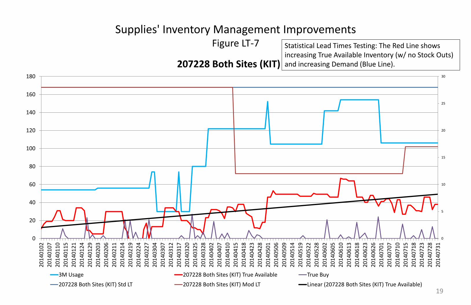
Supplies' Inventory Management Improvements Figure LT-7
0
5
10
15
20
25
30
0
20
40
60
80
100
120
140
160
180
20
14
01
02
20
14
01
07
20
14
01
10
20
14
01
15
20
14
01
21
20
14
01
24
20
14
01
29
20
14
02
03
20
14
02
06
20
14
02
11
20
14
02
14
20
14
02
19
20
14
02
24
20
14
02
27
20
14
03
04
20
14
03
07
20
14
03
12
20
14
03
17
20
14
03
20
20
14
03
25
20
14
03
28
20
14
04
02
20
14
04
07
20
14
04
10
20
14
04
15
20
14
04
18
20
14
04
23
20
14
04
28
20
14
05
01
20
14
05
06
20
14
05
09
20
14
05
14
20
14
05
19
20
14
05
22
20
14
05
28
20
14
06
02
20
14
06
05
20
14
06
10
20
14
06
13
20
14
06
18
20
14
06
23
20
14
06
26
20
14
07
01
20
14
07
07
20
14
07
10
20
14
07
15
20
14
07
18
20
14
07
23
20
14
07
28
20
14
07
31
207228 Both Sites (KIT)
3M Usage 207228 Both Sites (KIT) True Available True Buy
207228 Both Sites (KIT) Std LT 207228 Both Sites (KIT) Mod LT Linear (207228 Both Sites (KIT) True Available)
Statistical Lead Times Testing: The Red Line shows increasing True Available Inventory (w/ no Stock Outs) and increasing Demand (Blue Line).
19

Supplies' Inventory Management Improvements Figure LT-8
0
5
10
15
20
25
30
35
0
20
40
60
80
100
120
140
20
14
01
02
20
14
01
07
20
14
01
10
20
14
01
15
20
14
01
21
20
14
01
24
20
14
01
29
20
14
02
03
20
14
02
06
20
14
02
11
20
14
02
14
20
14
02
19
20
14
02
24
20
14
02
27
20
14
03
04
20
14
03
07
20
14
03
12
20
14
03
17
20
14
03
20
20
14
03
25
20
14
03
28
20
14
04
02
20
14
04
07
20
14
04
10
20
14
04
15
20
14
04
18
20
14
04
23
20
14
04
28
20
14
05
01
20
14
05
06
20
14
05
09
20
14
05
14
20
14
05
19
20
14
05
22
20
14
05
28
20
14
06
02
20
14
06
05
20
14
06
10
20
14
06
13
20
14
06
18
20
14
06
23
20
14
06
26
20
14
07
01
20
14
07
07
20
14
07
10
20
14
07
15
20
14
07
18
20
14
07
23
20
14
07
28
20
14
07
31
723418 Both Sites (KIT)
3M Usage 723418 Both Sites (KIT) True Available True Buy
723418 Both Sites (KIT) Std LT 723418 Both Sites (KIT) Mod LT Linear (723418 Both Sites (KIT) True Available)
Statistical Lead Times Testing: The Red Line shows increasing True Available Inventory (w/ no Stock Outs) and increasing Demand (Blue Line).
20

Supplies' Inventory Management Improvements
Demand accuracy is essential to the right balance between Service Level and Inventory Investment
• Many methods exist to estimate logistical Demand – from simple Statistics to sophisticated Numerical Methods.
• Developed a new method: A computer program that simulates the human judgment involved in estimating Stochastic Demand from monthly historical data.
• Program applies Numerical Methods to the task of Demand Estimation: Polynomial Regression, Numerical Integration, and Root Location.
• Program suppresses short-term Demand Spikes and Demand Surges, thereby preventing high-probability over-buying (Fig. D-1).
• Program factors Demand Trend and Change in Demand Trend into the Demand estimate (Fig. D-2).
21

Supplies' Inventory Management Improvements
Demand accuracy is essential to the right balance between Service Level and Inventory Investment
• So far, 150 / 150 automated Demand estimates have been confirmed by visual inspection.
• Program eliminates the time-consuming need to manually estimate Demand. Approximate Time Savings: 15 hours / month.
• Program operates on 12 months’ data and better optimizes inventory than a pure statistical approach because it applies human judgment in: (1) suppressing Transient conditions, and (2) capitalizing on Trend.
• A 12-month pure statistical approach produces an estimated 19.5 percent increase in inventory compared with the 12-month Numerical Method approach (Fig. D-3).
• Automated demand estimates will play an important role in transitioning all remaining Supplies' B- and C-Items to MRP.
22

Supplies' Inventory Management Improvements Figure D-1 Program suppresses short-term Demand spikes.
Red dot at right side of chart is the Numerical Demand Estimate.
Numerical Demand Estimate
0
100
200
300
400
500
600
700
800
0 1 2 3 4 5 6 7 8 9 10 11 12 13
Q(t
)
t
23

Supplies' Inventory Management Improvements Figure D-2 Program factors in Demand Trend and Change in Demand Trend.
Red dot at right side of chart is the Numerical Demand Estimate.
Numerical Demand Estimate
0
100
200
300
400
500
600
700
800
900
1000
0 1 2 3 4 5 6 7 8 9 10 11 12 13
Q(t
)
t
24
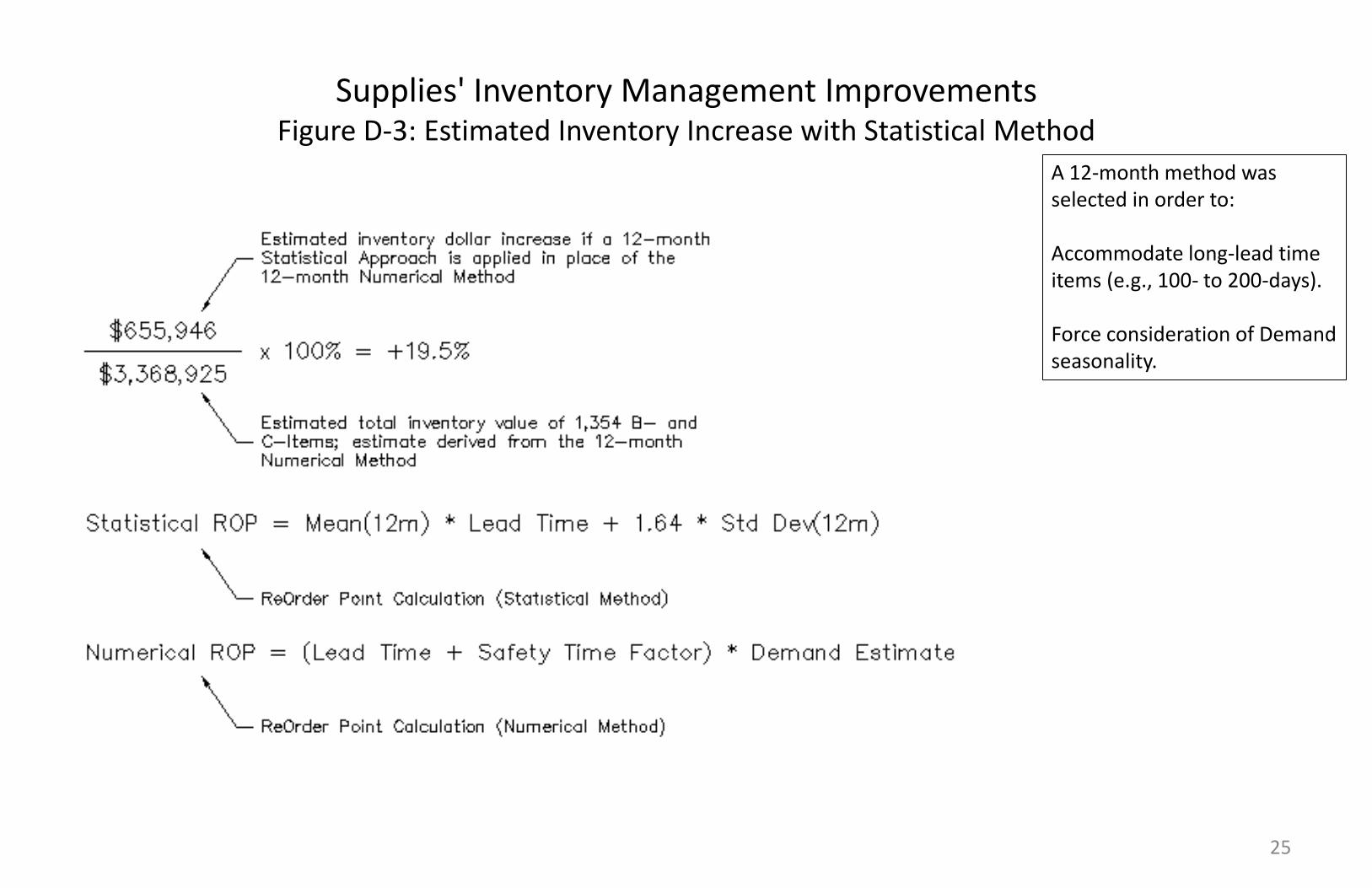
Supplies' Inventory Management Improvements Figure D-3: Estimated Inventory Increase with Statistical Method
A 12-month method was selected in order to: Accommodate long-lead time items (e.g., 100- to 200-days). Force consideration of Demand seasonality.
25

Supplies' Inventory Management Improvements
Future Improvements
• Place into service the newly-developed MRP parameters (i.e., ReOrder Points and Economic Order Quantities).
• Develop a computer program that facilitates efficient visual inspection of Statistical Lead Times and Demand estimates.
• Develop a report that identifies significant Trend in Lead Times and Demands.
• Develop a part-specific time-series report of Service Level and Inventory Investment.
• Develop a program that numerically determines the optimum combination of Lead Time, Demand, and Safety Stock parameters for part-specific Service Level and Inventory Investment.
26

Supplies' Inventory Management Improvements
Numerical Methods can generally be defined as Computer Math
• I have been developing Numerical Methods software since 2002 in the following areas: Engineering, Physics, Roots of Equations, Linear Algebraic Equations, Optimization, Curve Fitting, Calculus, and Business / Inventory Management.
• Due to Supplies‘ dependence on Excel, all programming was done in Visual BASIC for Applications/Excel.
• Learned Numerical Methods development from the Chapra/Canale text: Numerical Methods for Engineers, 4th Edition. Adhering to their requirements for high-quality software development:
1. Top-Down Design: Systematic development; i.e., general objectives w/ division into specific segments.
2. Modular Programming: Use of functions / subroutines within an organized and coherent scheme.
3. Structured Programming: Well-structured code IAW the three Control Structures: Sequence, Selection, Repetition.
4. Program Testing.
27