improving broad scale forage mapping and habitat selection...

Improving broad scale forage mappingand habitat selection analyses with airborne laser scanning:

the case of moose

KAREN LONE,1,� FLORIS M. VAN BEEST,2 ATLE MYSTERUD,3 TERJE GOBAKKEN,1 JOS M. MILNER,4,5

HANS-PETTER RUUD,1 AND LEIF EGIL LOE1

1Department of Ecology and Natural Resource Management, Norwegian University of Life Sciences, P.O. Box 5003,NO-1432 Aas, Norway

2Department of Bioscience, Aarhus University, Frederiksborgvej 399, 4000 Roskilde, Denmark3Centre for Ecological and Evolutionary Synthesis (CEES), Department of Biosciences, University of Oslo,

P.O. Box 1066 Blindern, NO-0316 Oslo, Norway4Hedmark University College, Department of Forestry and Wildlife Management, Campus Evenstad, NO-2480 Koppang, Norway

Citation: Lone, K., F. M. van Beest, A. Mysterud, T. Gobakken, J. M. Milner, H.-P. Ruud, and L. E. Loe. 2014. Improving

broad scale forage mapping and habitat selection analyses with airborne laser scanning: the case of moose. Ecosphere

5(11):144. http://dx.doi.org/10.1890/ES14-00156.1

Abstract. Determining the spatial distribution of large herbivores is a key challenge in ecology and

management. However, our ability to accurately predict this is often hampered by inadequate data on

available forage and structural cover. Airborne laser scanning (ALS) can give direct and detailed

measurements of vegetation structure. We assessed the effectiveness of ALS data to predict (1) the distribution

of browse forage resources and (2) moose (Alces alces) habitat selection in southern Norway. Using ground

reference data from 153 sampled forest stands, we predicted available browse biomass with predictor

variables from ALS and/or forest inventory. Browse models based on both ALS and forest inventory variables

performed better than either alone. Dominant tree species and development class of the forest stand remained

important predictor variables and were not replaced by the ALS variables. The increased explanatory power

from including ALS came from detection of canopy cover (negatively correlated with forage biomass) and

understory density (positively correlated with forage biomass). Improved forage estimates resulted in

improved predictive ability of moose resource selection functions (RSFs) at the landscape scale, but not at the

home range scale. However, when also including ALS cover variables (understory cover density and canopy

cover density) directly into the RSFs, we obtained the highest predictive ability, at both the landscape and

home range scales. Generally, moose selected for high browse biomass, low amount of understory vegetation

and for low or intermediate canopy cover depending on the time of day, season and scale of analyses. The

auxiliary information on vegetation structure from ALS improved the prediction of browse moderately, but

greatly improved the analysis of habitat selection, as it captured important functional gradients in the habitat

apart from forage. We conclude that ALS is an effective and valuable tool for wildlife managers and ecologists

to estimate the distribution of large herbivores.

Key words: Airborne laser scanning (ALS); Alces alces; cover; ecological indicators; habitat mapping; integration of

forest and wildlife management; LiDAR; Norway; population monitoring; remote sensing; Resource Selection Functions

(RSFs); ungulate management.

Received 30 May 2014; revised 23 August 2014; accepted 27 August 2014; final version received 18 September 2014;

published 24 November 2014. Corresponding Editor: R. R. Parmenter.

Copyright: � 2014 Lone et al. This is an open-access article distributed under the terms of the Creative Commons

Attribution License, which permits unrestricted use, distribution, and reproduction in any medium, provided the

original author and source are credited. http://creativecommons.org/licenses/by/3.0/5 Present address: School of Biological Sciences, University of Aberdeen, Tillydrone Avenue, Aberdeen AB24 2TZ United

Kingdom.

� E-mail: [email protected]

v www.esajournals.org 1 November 2014 v Volume 5(11) v Article 144

INTRODUCTION

Among ungulates, density-dependent foodlimitation is a main limiting factor in populationdynamics (Bonenfant et al. 2009). Forage qualityand quantity are therefore important determi-nants of foraging and habitat selection patterns oflarge herbivores (Fryxell 1991, Hanley 1997).Despite the strong influence of food resources onboth habitat selection and population dynamics,quantification of food availability at large spatialscales remains challenging. Most studies rely onenvironmental proxies of forage availability andcover, such as NDVI (Mueller et al. 2008), landcover classes (Uzal et al. 2013), or forest standcharacteristics like productivity (Godvik et al.2009), dominant tree species (Dussault et al.2005a) and age class (Mabille et al. 2012). Often,such proxies are used without quantifying levelsof food and cover, though exceptions occur (vanBeest et al. 2010b, Avgar et al. 2013, Blix et al.2014). It is well known that the physical structureof the habitat is also important for habitatselection as cover is used for concealment andthermal shelter (Mysterud and Østbye 1999,DePerno et al. 2003).

Scale matters greatly in the study of ecologicalphenomena (Wiens 1989). Habitat selectionpatterns often differ between scales, reflectingprocesses and behavioral decisions operating atdifferent scales (Boyce et al. 2003, DeCesare et al.2012). The scale of the study should reflect thequestion at hand. The concept of scale involvesboth extent of the study area, the resolution of thedata, and in some cases, the range over which theenvironmental context is considered (De Knegt etal. 2011). In wildlife management, importantquestions on a broad scale include identifying apopulation’s seasonal range use or what land-scape elements are important within an animal’shome range. GPS tracking collars for wildlifehave enabled researchers to collect large quanti-ties of precise location data covering large areas.On the other hand, environmental data coveringthe same broad scales often have low resolutionand precision (such as GIS-based land useclasses). This discrepancy frequently results inpoor predictive ability of habitat selection models(Loe et al. 2012). New methods for monitoringforage resources and physical habitat structurewith fine resolution at broad scales are therefore

of considerable interest for both basic andapplied ecological research.

Airborne laser scanning (ALS) is a promisingremote sensing technique for obtaining habitatinformation across large spatial scales. Besidesproviding detailed elevation models, these datahold three-dimensional information on the dis-tribution of vegetation biomass. Forest parame-ters such as timber volume and stem density canbe estimated with high precision, and theseprocedures have been operational in the Scandi-navian countries for more than ten years(Holmgren 2004, Næsset 2004). ALS data arealso increasingly applied in large-scale ecosystemstudies (Lefsky et al. 2002), to estimate carbonstorage (Stephens et al. 2007), biodiversity(Muller and Vierling 2014), to map standingdead wood (Pesonen et al. 2008) and to modelhabitat for various wildlife species (Hill et al.2014), including birds (Hinsley et al. 2002) andungulates (Coops et al. 2010, Melin et al. 2013,Lone et al. 2014). In these studies, laser data havebeen used directly to interpret the physicalstructure of the habitat relevant to each speciesor species assemblages. Despite the fundamentalimportance of forage and cover in understandinganimal ecology, there has been no formal analysislinking structural information of habitat to forageresources, and few relating ALS derived covervariables to habitat selection (Graf et al. 2009,Melin et al. 2014).

The aim of this study was twofold: (1) toevaluate the use of ALS data in quantifying andpredicting biomass of browse species common inthe diet of Norwegian moose (Alces alces), and (2)to determine whether ALS-derived measures offorage and physical habitat structure (cover) areeffective in predicting habitat selection of mooseat multiple spatial and temporal scales. Moose inScandinavia are partially migratory and typicallymigrate from high elevation summer habitats tolow elevation winter habitats that have highavailability of browse (commonly young pinestands) and more favorable snow conditions(Ball et al. 2001, Nikula et al. 2004). Moosehabitat selection is related to forage availabilityand cover, both at the landscape and home-rangescales (Dussault et al. 2005b, Mansson et al. 2007,Herfindal et al. 2009, van Beest et al. 2010b). At alandscape scale, moose select home ranges withlarge volumes of biomass, while they tend to


LONE ET AL.

select for forage quality within home ranges (vanBeest et al. 2010b). The moose represents an idealmodel species to test the applicability of ALSbecause its food (mainly browse) is found in thebush and tree strata (Mysterud 2000), which canpotentially be quantified with ALS data. Here,we build upon the study by van Beest et al.(2010b), in which forage distribution was mod-eled using forest stand-based inventory andterrain data. Using that dataset in combinationwith existing ALS data, we tested whether thepredictive forage models were improved byincluding ALS-derived variables, and whetherALS data could predict browse biomass well onits own. Finally, we evaluated the usefulness ofthe spatial predictions of browse biomass andselected ALS variables in resource selectionfunctions (RSFs) for GPS-marked moose insouthern Norway.

METHODS

Study area and the study speciesThe study was conducted in an 1100-km2 area

within Telemark and Vestfold counties in south-ern Norway (Appendix: Fig. A1). The area iswithin the southern boreal to boreonemoralzones. Land cover is dominated by commerciallymanaged forests of Norway spruce (Picea abies)and Scots pine (Pinus sylvestris). Some mixeddeciduous stands of birch species (Betula pubes-cens and B. pendula), rowan (Sorbus aucuparia),willow (Salix spp.) and aspen (Populus tremula)occur throughout the area. The mean monthlytemperatures in June and January are 15 and�58C, respectively (Siljan weather station at 100m above sea level [asl], The Norwegian Meteo-rological Institute; http:// www.met.no). Snowdepths (mean 6 SD) at a 430 m asl locationduring January–April 2007 and 2008 were 42 6

29 cm and 73 6 21 cm (Mykle weather station,The Norwegian Meteorological Institute). Moosedensities in the area were estimated at 1.3individuals/km2 (Milner et al. 2012), but percapita available browse is low relative to its peakin the 1960s (Milner et al. 2013).

Field measured browse biomassField estimates of browse forage biomass were

made for six tree species: pine, silver birch,downy birch, rowan, aspen, and goat willow

(Salix caprea). These species represent the mostpreferred species and, together with the erica-ceous shrub bilberry (Vaccinium myrtillus), thebulk of what moose feed on in both summer andwinter. In the original field-study 189 foreststands were sampled using a random stratifiedsampling design (van Beest et al. 2010b). Becausethe ALS data did not cover the entire originalstudy area, data from only 153 forest stands wereused here, but these were well spread among theoriginally chosen strata: development class (5class factor: 1 ¼ forest under regeneration, 2 ¼regenerated areas and young forest, 3 ¼ youngthinning stands, 4 ¼ advanced thinning stands,and 5 ¼mature forest), dominant tree species (3class factor: Scots pine, Norway spruce andmixed deciduous), and aspect (4 class factor:north, east, south and west). Each forest standwas sampled with five 50-m2 circular subplots,and the center coordinates of the central subplotwere recorded with a handheld GPS obtaining anaverage location over 10 min or more. Based onexperience from GPS measurements of almost1000 plots in similar forest areas we expect amean location error from the true position of lessthan 3.5 m with a standard deviation of less than3 m (O. M. Bollandsas, E. Næsset, and T.Gobakken, unpublished data). The four remainingsubplots were placed 25 m away from the centersubplot in each of the four cardinal directions,and were at least 15 m from the edge of the foreststand. Within each subplot, the canopy volumeand stem diameter of individual trees of thetarget species were measured in order to predictthe leaf (summer) or twig (winter) biomassaccessible to moose (,3.0 m height, and account-ing for snow cover in winter) using allometricmodels. The R2 of the allometric models ofavailable browse ranged from 0.63 to 0.92 (seevan Beest et al. 2010b for more details on theallometric models). Rowan, aspen and willowsare high quality but relatively less commonbrowse species that were considered together asone category of browse (abbreviated as RAW).Total forage biomass in winter (twigs) includedall six browse species while summer foragebiomass (leaves) included all species except pineas moose do not forage on it during summer. Theaverage biomass of the five 50-m2 subplots wasconsidered as the ground reference biomass for2500-m2 circular plots that encompassed the


LONE ET AL.

subplots (Table 1). We chose to model biomass atthis scale (2500 m2) because it gave the bestspatial match between the ground reference dataand the ALS data, given the georeferencinginaccuracies of the field data material. Therewas considerable variability in the responsevariables between subplots within each plot,and although the between-plot variability wasgreater, the subsampling procedure likely intro-duced some noise in the response variable on the2500-m2 plot (Table 1).

Forest inventory dataWe had access to the stand-based forest

inventory for operational forest managementfor a large (40–80%) and fairly contiguousportion of the forested area in the municipalitieswe considered. Maps were available in Geo-graphic Information System software and includ-ed information on stand delineations (polygons)and associated stand-level attributes: dominanttree species (deciduous, spruce, pine), develop-ment class (1–5) and h40 site index (SI) ofproductivity (defined in Tveite 1977). Productiv-ity was reclassified as a two-level factor: ‘‘high’’where SI . 14 and ‘‘low’’ where SI � 14. Fieldassessment confirmed that the accuracy of themaps was high (van Beest et al. 2010a).

ALS dataLaser scanning systems developed for airborne

platforms are used to survey large areas in greatdetail. A laser beam with a small footprint isdirected towards the ground in pulses, andscanned across the landscape perpendicular tothe flight direction. Each flight line thus covers astrip of land, and the flight pattern can be

planned so each strip overlaps with the next togive continuous cover over the entire study area,as in this study. For each laser pulse, the ALSinstrument registers one or more peaks in thereturn signal. From the position of the aircraft,the speed of light and the reflection time of eachregistered peak in the return signal, the systemcalculates the location where the beam wasreflected from (see Wehr and Lohr 1999 for atechnically detailed description). This yields adata set of ‘echoes’ from ground, vegetation orman-made structures with accurate X, Y, and Zcoordinates, out of which the ground echoes areclassified by standard algorithms (Axelsson2000). Commercial providers of laser data wouldnormally process the data to this stage wherethey are accessible to researchers in a specializedGIS environment, but do not require expertise ingeomatics.

The laser data were collected for other pur-poses and as four separate projects in the period2008–2010 (Appendix: Table A1). Project param-eters were similar for the three projects withrelatively low pulse density (1–2 m�2), while thefourth had a higher pulse density (12 m�2) due toa lower flying altitude, smaller scan angle, andhigher pulse frequency than the other threeprojects. As the higher quality data in one regioncould potentially have affected results, we testedthis possibility in the final models and found thatnone were significantly improved by includinginteractions between the ALS variables andregion/laser project. Each project was deliveredfrom the contractor as a point cloud with UTMcoordinates and ellipsoidal height, with groundechoes classified. A triangular irregular network(TIN) representing the ground surface was madefrom the ground echoes and subtracted from theZ coordinates of the point cloud, to give heightabove ground (dz) for each echo. From theground surface TIN, we derived a digital terrainmodel (DTM) with a 10-m cell size, and used it tocalculate slope, aspect and hill shade. For eachfield plot, the corresponding ALS echoes wereextracted from circular plots of 2500 m2 centeredon the ground reference field plots, thus encom-passing the five subplots. Variables describingthe vertical distribution of the echoes werecalculated for each plot. These were summarystatistics of the height values: the 10th, 20th, 30th,. . . , 90th percentiles, mean, max, standard

Table 1. Summary statistics for the response variable

browse biomass (g/m2) at the 2500-m2 plot level and

the mean standard deviation (SD) of the five

subplots.

Variable Mean Min Max SDWithin-plot

SD

RAW (winter) 39.0 0 419 71.8 33.9RAW (summer) 83.6 0 1021 152 62.1Pine (winter) 157 0 2710 383 168Total biomass (winter) 331 0 3286 524 311Total biomass (summer) 158 0 1165 215 104

Note: RAWdenotes a group of high quality browse species:rowan, aspen and goat willow.


LONE ET AL.

deviation and coefficient of variation of theheight of echoes with dz . 0.5 m. Additionally,the proportion of echoes within the heightintervals corresponding to ground, understoryand canopy: 0–0.5 m, 0.5–3.0 m, above 3.0 m(thus a measure of canopy cover), and, lastly, theratio of understory echoes (0.5 m , dz � 2.0 m)to understory and ground echoes (dz � 2.0 m) (ameasure of understory cover). Wing et al. (2012)also utilized echo intensity to distinguish groundand vegetation echoes, but as we lacked calibrat-ed intensity measures our definition of understo-ry cover relied solely on echo height. Many of theALS variables are correlated, and to aid modelinterpretation, we pre-screened them to avoidcross-correlation (r . 0.5), retaining the function-ally most meaningful variables: canopy cover,understory cover, 90th percentile of height (h90)and coefficient of variation of height (hcv). Asingle pulse can give several echoes, and we usedall echoes in the calculation of the variables inorder to use all the information and becauseinitial analyses showed better results than split-ting into first and last echoes. Terrain variableswere extracted from the cell that each plot centerfell in.

Browse biomass modelsWe developed models for summer and winter

biomass of RAW, winter biomass of pine, andtotal summer biomass and total winter biomassseparately. To fulfill the assumption of homoge-neity of the variance, we used log-linear regres-sions to model the available forage biomass. Weused three sets of predictor variables, inventoryvariables alone, inventory and ALS variablestogether, and ALS variables alone. Terrainvariables (elevation, slope, aspect and hill shade)were always included as topography influencesgrowing conditions (Gartlan et al. 1986). Weallowed for an interaction between h90 andcanopy cover. Understory cover was log-trans-formed. For each of the three sets of candidatepredictor variables, we identified the best modelby backwards selection using F-tests with cutoffp¼ 0.05 (Murtaugh 2009). We assessed predictiveperformance using K-fold cross-validation withfive folds, fitting the model to 80% of the dataand using it to predict observations for theremaining 20%. From this, we determined thevariation explained by the model using squared

Pearson’s correlation coefficient between log-transformed responses and predictions on logscale. We assessed prediction accuracy by calcu-lating the root-mean-square prediction error(RMSPE) for predictions, both on the log scaleand back-transformed. We extrapolated ourresults to map total available moose forage inwinter and summer across the study area. A gridwith 50 m3 50 m cells was superimposed on theALS point cloud and for each cell we calculatedthe variables describing the vertical distributionof echoes using the same definitions as for thefield plots. The resulting ALS raster maps wereused together with the rasterized forest inventoryvariables to predict, cell by cell, the availablebrowse biomass according to the final models fortotal winter biomass and total summer biomass.We applied the bias-correction factor of Snowdon(1991) to all predictions: after back-transforma-tion from the log scale, they were multiplied bythe ratio of the average value of responsevariables on the original scale to the averagevalue of the predicted values after back-transfor-mation. All analyses were done in R 2.14.1 (RDevelopment Core Team 2011).

Moose dataIn total 34 adult female moose were tranquil-

ized by dart gun from a helicopter, usingestablished techniques (Arnemo et al. 2003),and fitted with GPS collars (Tellus RemoteGSM, Followit AB, Lindesberg, Sweden) pro-grammed with a 1 hour relocation schedule. Allanimal handling was carried out with permissionfrom the national management authority, theDirectorate for Nature Management (protocolnumber: FOTS ID 1428), and evaluated andapproved in accordance with the ethical guide-lines and legal requirements set by the Norwe-gian Institute for Nature Research. Collar datawere collected from January to November 2007(n¼16) and 2008 (n¼18) but the sample size wasreduced to 31 individuals during winter and to20 individuals during summer due to collarmalfunctions and exclusion of individuals withseasonal space use outside the area of ALScoverage. All GPS locations collected within 24h of marking were excluded. Winter length wasdefined based on snow conditions (period with�30 cm snow depth). In 2007 winter stretchedfrom 21 January until 8 April and in 2008 from 4


LONE ET AL.

January until 30 April. We defined summer as 1June until 15 September for both years, andexcluded spring and autumn positions altogeth-er. The average GPS-collar fix rate was 96%(range 87–99%) during winter and 90% (range83–97%) during summer. To correct for possiblebias in GPS fix success prior to analyzing habitatselection, we simulated the missing GPS posi-tions weighting by the terrain-specific probabilityof obtaining a fix (Frair et al. 2004, van Beest et al.2010b).

Moose habitat selection analysisTo evaluate how effectively the forage maps

and ALS information quantified habitat selectionof moose, we used RSFs and followed proceduresin van Beest et al. (2010b) as closely as possible.RSFs are defined as any function proportional tothe probability of use of a resource unit by ananimal (Manly et al. 2002). We computed RSFsfor both summer and winter seasons and for twospatial scales commonly investigated in basic andapplied ecology: where in the landscape seasonalhome ranges are located and where withinseasonal home ranges the animals spend time,i.e., second and third selection order of Johnson(1980). As such, habitat availability at the withinhome range scale was estimated by drawing arandom sample of point locations from withineach individual’s wintering and summer home

range (delineated by a 95% minimum convexpolygon). Available points were selected in equalnumber to the used points for each individual. Atthe landscape scale, habitat availability wasdefined as a random sample of point locationsfrom within the study area boundaries and weconsidered availability at the within home rangescale as used points (Aebischer et al. 1993). Foreach spatiotemporal scale, we compared sixcandidate RSFs (Table 2) that had forest inven-tory data, predicted forage availability, ALSestimates of canopy and understory cover, orsome combination of these as predictor variables.The resource (predictor variable) value at a usedor available point location was extracted from the2500-m2 cell of the resource map that the pointfell within. A preliminary analysis showed a non-linear relationship with selection so we includeda second order effect of canopy cover. At thehome range scale we included interactionsbetween all focal predictor variables and lightcondition (dark, daylight, twilight) as mooseactivity level depended on light conditions(highest activity levels during twilight; F. M.van Beest and J. M. Milner, unpublished data) andthis may be related to resource use. Candidatemodels were selected a priori to assess whetherthe ALS variables improved the predictive abilityof the RSFs, either directly by quantifying cover,or through better forage estimates.

Table 2. The candidate moose RSF models compared within each combination of season and scale and the

interpretation of specific inter-model comparisons.

Modelno. Data origin

Focal predictorvariables Evaluation and interpretation

1 Forest inventory maps development class,dominant species

If best model, ALS information doesn’t contributeanything new to moose selection models and foreststand classes capture moose selection better thansimple functional gradients of total forage biomass ortotal amount of cover

2 Forage maps (inventory) total forage biomass If best model, ALS information doesn’t contributeanything new to moose selection models and totalforage biomass is the main driver of selection patterns

3 Forage maps (ALS) total forage biomass If nearly as good as model 2, ALS-only forage mapscapture the wildlife-relevant variation in forage as wellas other forage maps

4 Forage maps (inventory &ALS)

total forage biomass If better than model 2, ALS-improved forage maps leadto improved predictions of moose space use

5 ALS variables canopy cover, understorycover

If best model, ALS vegetation structure variables captureimportant habitat variation better than the forageestimates or the inventory categories, by capturing thesame and/or additional information

6 Forage maps (inventory)and ALS variables

total forage biomass,canopy cover,understory cover

If better than model 4, ALS holds information relevantto moose habitat selection beyond how it relates toforage


LONE ET AL.

Coefficients of the exponential RSFs wereestimated from use–availability data in amixed-effects logistic regression (design III data;Thomas and Taylor 2006) with moose ID as arandom intercept (Gillies et al. 2006). Mixed-effect logistic regressions were fitted using thelibrary ‘lme4’ (Bates et al. 2012) implemented inR (R Development Core Team 2011). For eachspatiotemporal scale, we compared the fit (usingAIC) and predictive performance (with K-foldvalidation; Boyce et al. 2002) of the six pre-defined candidate RSFs. For the K-fold cross-validation procedure, the model was repeatedlytrained withholding 20% of the used locationsevery time. The points withheld for validationwere then predicted using that model and theirRSF scores were binned into ten bins that eachrepresented an equal area, as calculated from theavailable locations. We calculated the Spearman-rank correlation (rs) between the number ofpredicted used points in each bin and the binrank from low to high RSF score (Boyce et al.2002). This procedure was repeated 100 times todetermine whether the rs was significantlydifferent from random.

RESULTS

Estimating biomass of browse forageThe explanatory power (R2) of the best forage

models for each browse category ranged from0.35 to 0.58, while the K-fold cross-validatedPearson r2 ranged from 0.28 to 0.50 (Table 3). Allmodels tended to over-predict at low biomassand under-predict at higher biomass, so theestimated quantity is better interpreted as arelative rather than an absolute measure offorage biomass (Appendix: Fig. A2). Modelsincluding ALS variables typically had morepredictor variables. To ensure that the improve-ment was not only due to the increased com-plexity of the model, we made our comparisonon the basis of the cross-validation Pearson r2

and RMSPE. The models including both ALS andinventory variables predicted as well or betterthan the inventory-only models. By includingALS variables, we could explain 7 percentagepoints and 6 percentage points more of thevariation in total biomass for winter and sum-mer, respectively, bringing the explained varia-tion up to 45% and 28% (Table 3). The prediction

Table 3. Predictive ability of the best browse biomass models using inventory (inv), airborne laser scanning

(ALS), or inventory and ALS data; explained variation (R2), cross-validated explained variation (Pearson r2),

root mean square prediction error normalized to the mean value of the response (RMSPE %), and number of

estimated parameters (k).

Data type R2Cross-validation�

Pearson r2Cross-validation�

RMSPE (%)Cross-validation�

RMSPE (%) k

RAW (winter)inv 0.32 0.26 65.8 158 7inv þ ALS 0.37 0.29 64.7 151 10ALS 0.18 0.15 70.5 175 4

RAW (summer)inv 0.33 0.28 52.9 159 7inv þ ALS 0.36 0.29 52.6 158 11ALS 0.10 0.09 59.2 176 1

Pine (winter)inv 0.56 0.50 68.7 217 7inv þ ALS 0.58 0.50 68.3 209 8ALS 0.23 0.18 87.6 248 4

Total biomass (winter)inv 0.45 0.38 33.5 145 (145) 8inv þ ALS 0.52 0.45 31.5 151 (144) 11ALS 0.30 0.24 37.0 176 (178) 5

Total biomass (summer)inv 0.30 0.22 32.3 121 8inv þ ALS 0.35 0.28 30.9 117 9ALS 0.18 0.13 33.8 134 5

Notes: RAW¼rowan, aspen and goat willow. For total biomass winter the RMSPE of the back-transformed predictions withone influential point removed is shown in parentheses.

� Calculated with log-transformed responses and predictions on log scale.� Calculated with untransformed responses and back-transformed predictions.


LONE ET AL.

of biomass was not improved for pine, while itwas slightly improved for the RAW species.Models that only used ALS variables hadconsistently poorer predictive abilities than eitherof the models including inventory variables(Table 3).

ALS variables were generally included inaddition to the other variables, rather thanoutperforming them. In particular, ALS variablesnever replaced the inventory variables dominanttree species and development class, which werekept in nearly all relevant top models (Table 4).The important ALS variables were canopy cover,h90 in interaction with canopy cover, andunderstory cover. For total biomass in winterand summer, increasing ALS measured canopycover was negatively correlated with forageavailability (Fig. 1). For total biomass in winter,the steepness of this slope depended on thegeneral height of the trees (h90), where tallertrees meant a steeper decline in forage availabil-ity with canopy cover. An increase in understorycover was related to an increase in availableforage biomass (Fig. 1). This was the case for allmodels where understory cover was included(Table 4).

The final product of browse modeling wassummer and winter forage maps, based on ALSand/or inventory data. Fig. 2 shows maps basedon the best models using inventory and ALS data.

Habitat selection of mooseOverall, the best performing RSF models were

those containing ALS variables (models 5 and 6),both in terms of AIC rank and K-fold validation(Table 5). Although the RSFs based on the forestinventory maps only (model 1) often hadrelatively low AIC values, the K-fold validationshowed that these models had low predictivepower. The RSFs based on forage maps predictedonly by means of ALS (model 3) were neverranked as the top-model. Moose selected for alow or intermediate amount of canopy coverdepending on the time of day, season and spatialscale of analyses, and typically against (andnever for) understory cover (Fig. 3; Tables A2–A5). At the landscape scale, moose selected forlow canopy cover both during summer andwinter (Fig. 3A, B). At the home range scale,moose selected for an intermediate optimum ofcanopy cover during daytime (Fig. 3C, D). Attwilight and night, moose selected sites withlower canopy cover as low canopy cover wasmonotonically selected (summer: Fig. 3F, H) orthe optimum was shifted to lower canopy coverrelative to the daytime optimum (winter: Fig.3E, G). Moose selected for sites with increasedforage biomass in all seasons and times of day atboth the landscape scale and the within homerange scale (all b . 0, all p , 0.05; Appendix:Tables A2–A5).

Table 4. The best models for predicting available forage biomass by browse category.

Predictor variable

RAW Pine Total biomass

Winter Summer Winter Winter Summer

b SE b SE b SE b SE b SE

(Intercept) 3.30 0.97 3.80 1.1 3.09 0.60 6.32 0.94 6.76 0.65Dominant tree species�

Pine �1.85 0.34 �2.42 0.40 1.93 0.40 0.31 0.35 �1.27 0.32Spruce �0.96 0.33 �0.69 0.36 �1.25 0.37 �1.28 0.32 �1.11 0.29

Development class�2 �0.60 0.37 �0.35 0.41 0.43 0.43 0.85 0.36 0.24 0.333 �0.78 0.39 �0.65 0.43 �0.98 0.43 �0.40 0.38 �0.52 0.334 0.06 0.39 0.57 0.43 �1.25 0.45 �0.05 0.38 0.26 0.345 �0.87 0.39 �0.63 0.43 �1.74 0.46 �1.15 0.38 �1.10 0.34

Productivity§Low . . . . . . 0.71 0.37 1.24 0.36 0.83 0.33 0.91 0.27

h90 0.18 0.08 0.15 0.083 . . . . . . 0.070 0.073 . . . . . .Canopy cover 4.82 1.92 2.88 2.3 �2.06 0.83 0.88 2.0 �2.61 0.65h90:canopy cover �0.40 0.13 �0.31 0.15 . . . . . . �0.26 0.13 . . . . . .log(understory cover) 0.53 0.19 0.43 0.21 . . . . . . 0.51 0.18 0.32 0.15

Note: RAW¼ rowan, aspen and goat willow.� Reference level ¼mixed deciduous stands.� Reference level¼ development class 1.§ Reference level¼ high productivity.


LONE ET AL.

DISCUSSION

The lack of broad scale information on forageand cover availability has often hamperedstudies of spatial distribution of large herbivores,as field-based inventories of forage at largespatial and temporal scales are extremely costlyand rarely available. Remote sensing techniqueshave great potential to fill this void as they canextract detailed information on biotic or abioticenvironmental conditions relevant to ecologicalstudies (Pettorelli et al. 2014). Here, we presenteda novel use of ALS data to model browse

availability at the landscape scale in a managedboreal forest. Incorporating ALS data moderatelyimproved models predicting browse biomasscompared to models only using inventory mapinformation. A significant challenge in our studywas to fully exploit the potential of ALSinformation to estimate forage due to limitationsin matching laser data to field data. This resultedin only conservative improvements in predictiveability. Nonetheless, ALS is a promising tool forquantifying forage for large browsers such asmoose. Our study further showed that the ALS-based structural information on cover increased

Fig. 1. Predicted effects of airborne laser scanning variables on amount of available forage, from the best

models for total biomass in winter and summer (shown for deciduous stands of development class 2 with high

productivity). Shaded regions are 95% confidence intervals. For total winter biomass, effect of canopy cover is

shown for two values of 90th percentile echo height (h90) to show the interaction of the two variables. In that

panel, black is for h90¼ 11 m, grey is for h90¼ 17 m, this corresponds to the 20th and 80th percentiles of h90 in

the entire dataset. Rugplots along the x-axis show the distribution of the data.


LONE ET AL.

the predictive performance of moose habitatselection models. The possibility to obtain de-tailed and continuous maps of ‘‘new’’ environ-mental descriptors from ALS data offers greatopportunities across a range of research disci-plines in ecology, natural resource managementand conservation (Graf et al. 2009, Martinuzzi etal. 2009, Wing et al. 2012).

The effectiveness of ALS to quantify browseat broad scales

ALS increased explanatory power in thebrowse models by capturing variability in cano-py cover and density of understory vegetationwithin and between forest stands of a givencombination of development class and dominanttree species. Increasing canopy cover led to loweravailable forage biomass. This harmonizes withthe general ecological and silvicultural under-

standing that canopy gaps alter understoryconditions by increasing light levels (Canham1988) in favor of early colonizing species, such asthe forage species considered here. The interac-tion between h90 (the 90th percentile height ofnon-ground laser echoes) and canopy cover insome of the models may be an expression of‘‘effective openness’’ that depends on both theheight of the trees and canopy density. At thesame percentage canopy cover, shorter trees willshade less than tall trees and therefore beassociated with a greater effective openness. Incontrast to canopy cover, the ALS measuredunderstory cover also had a strong positiverelationship with forage biomass. This is expect-ed as understory cover consists of forage treespecies within browsing range of the moose.Among remote sensing technologies, ALS isuniquely suited to obtain such information on

Fig. 2. Maps of predicted browse availability in the study area in southern Norway. Areas with no forest

inventory data are shaded black, and include both non-forested land and forests under different ownership.


LONE ET AL.

the amount of understory, as some of the narrowlaser beams are able to penetrate through smallgaps in the canopy, even when it is relativelydense.

Boreal forest ecosystems are dynamic land-scapes with successional processes having aconsiderable impact on the physical structureand hence wildlife forage availability, includingbrowse (Angelstam and Kuuluvainen 2004).Although natural processes such as fire andstorms can open up forest canopies, Scandina-vian forest dynamics are largely determined bysilvicultural practices and clear-cutting (Kuulu-vainen and Aakala 2011). Indeed, the inventoryvariables forest development class and treespecies were never replaced by ALS variables inthe best models, which likely reflected theimportance of forestry practices in the dynamicsof wildlife forage availability. Although h90 is agood overall measure of vegetation height(Næsset and Bjerknes 2001), and thus thedevelopment from young to old forests, thecategorical representation of stand age andstructure as development class in the inventorymaps performed better in the models. While ALScan identify vegetation in the understory range,distinguishing between preferred and non-pre-ferred species or inedible material is more

difficult. Because of this, the improvement wefound in tree species-specific models was mar-ginal compared to the improvement on totalbrowse biomass estimates. That none of the ALSvariables could be interpreted in terms of treespecies composition, was probably the mainreason that the ALS-only model did not performsatisfactorily. As an alternative to using inventorydata as we did here, information on tree speciescould be obtained using other remote sensingtechniques. Although there are no readily avail-able ALS proxy measures of species composition,it can be modeled by ALS data if one alsoconsiders echo intensity measures (Brandtberg2007, Suratno et al. 2009, Ørka et al. 2013).Unfortunately, our ALS data did not havecalibrated intensity measures. Combining ALSwith multi- or hyperspectral images is anotheroption for obtaining reliable species classification(Holmgren et al. 2008, Ørka et al. 2013). In theScandinavian forest management context, devel-opment class, dominant tree species, site produc-tivity and stand delineations are typicallyobtained from stereographic photo interpreta-tion. As ALS forest inventories commonly rely onthis information (Næsset 2004), developmentclass and tree species would be readily availablecovariates if browse was estimated in conjunction

Table 5. Model fit according to AIC and model predictive performance according to K-fold cross-validation.

Scale Season Model no. k AIC DAIC AIC Wt LL K-fold rs

Landscape Winter 6 6 120887.8 0 1 �60437.88 0.835 5 120935.5 47.7 0 �60462.75 0.791 8 122320.7 1432.9 0 �61152.33 0.172 3 122531.3 1643.5 0 �61262.65 0.674 3 122648.8 1761.0 0 �61321.41 0.733 3 122721.5 1833.7 0 �61357.77 0.09�

Landscape Summer 6 6 71259.1 0 1 �35623.55 0.995 5 71285.9 26.8 0 �35637.92 0.991 8 71322.1 63.0 0 �35653.05 0.313 3 72830.3 1571.2 0 �36412.14 0.804 3 73091.4 1832.3 0 �36542.69 0.572 3 73167.4 1908.3 0 �36580.68 0.50

Home range Winter 6 16 124807.0 0 1 �62387.50 1.001 22 125766.5 959.5 0 �62861.25 0.595 13 126421.6 1614.6 0 �63197.81 1.002 7 127510.9 2703.9 0 �63748.47 0.924 7 128037.0 3230.0 0 �64011.52 0.783 7 129598.6 4791.6 0 �64792.32 0.82

Home range Summer 6 16 88182.2 0 1 �44075.11 0.975 13 88423.8 241.4 0 �44198.87 0.981 22 88814.0 631.8 0 �44385.01 0.594 7 89395.5 1213.3 0 �44690.74 0.712 7 89777.6 1595.2 0 �44881.80 0.813 7 90279.4 2097.2 0 �45132.69 0.82

Note: The models with the best K-fold values within each spatiotemporal scale are shown in boldface.� K-fold values that were not better than random (two-sample t-test, p . 0.05).


LONE ET AL.

with this.

ALS can be a viable stand-alone alternative if it

can predict browse availability without a sub-

stantial drop in performance relative to the

inventory data. The predictive power of the

models based on only ALS was too low to

promote this as based on the current study, yet it

should not be excluded until tested under

optimal field sampling design. Here we aimed

to best exploit existing field data, with the

drawback that survey grade GPS receivers were

not used for plot positioning and only 10% of the

ALS plot area was measured in the field.

Furthermore, the four ALS projects were collect-

ed over a three year time span and were collected

with different acquisition settings. Addressing

Fig. 3. Relative probability of selection of canopy cover by moose in southern Norway by season, scale and

light condition. Panels show landscape scale (A, B) and home range scale during daylight (C, D), twilight (E, F)

and darkness (G, H). Note that y-axis values (relative probability of selection) can be compared within, but not

between models.


LONE ET AL.

these issues in future studies would reduce thenoise in the data (Gobakken and Næsset 2009)with the expected consequence that ALS vari-ables would capture more of the variation andthus further improve predictions of browsecompared to our findings.

ALS improves understanding of habitat selectionIn addition to forage, we framed our habitat

selection analyses specifically around the conceptof cover, which is an important structuralelement of the habitat as it modifies interactionswith conspecifics or predators due to reducedvisual detection rates or hindrances in escaping(Schooley et al. 1996, Heithaus et al. 2009, Campet al. 2013). Moreover, cover affects food avail-ability and abiotic factors such as temperature,wind speed, humidity, snow depth and precip-itation (Mysterud and Østbye 1999). Our studyshows that incorporating ALS data improvedhabitat selection models of moose. The maincontribution towards this result was throughquantification of cover, rather than the improve-ment in forage predictions. Direct inclusion ofstructural variables is a common approach toALS based habitat studies (Graf et al. 2009,Coops et al. 2010, Melin et al. 2013), but theecological links are not always obvious. Habitatselection studies that lack detailed field data onforage and cover availability typically character-ize habitat as ‘‘open’’ or ‘‘dense’’ (Godvik et al.2009, Ciuti et al. 2012, Tolon et al. 2012) andassume these are ‘‘forage’’ and ‘‘cover’’ habitattypes respectively. There are clear drawbacks tothis, as we can expect variation in selectionwithin habitat types (Blix et al. 2014) linked tovariation in one or multiple resources or charac-teristics within a habitat type. By using ALSinstead of subjective habitat classes, we havedecoupled the physical structure of the habitatfrom other resources, and moved towards adirect investigation of animals’ habitat selectionon a functional gradient in cover that is fullyquantitative. Moose in our study avoided standswith dense understory vegetation, implying thatthey avoid visual shelter at ground level and (atleast weakly) high forage availability. Althoughthe reason for this finding remains unclear itcould be related to understory vegetation creat-ing movement obstructions or reducing theoverview of the surroundings (Camp et al.

2013). The selection for open canopy at thelandscape scale likely reflected selection foryoung forest stands, which is to be expected asmoose select for forage quantity at this scale (vanBeest et al. 2010b). At the within home rangescale, we observed a diurnal shift in use of cover.In daytime, selection peaked at an intermediatelevel of canopy cover. At intermediate levels,animals limited their exposure to wind, sun, rain,and humans, while actively selecting for forageunder these conditions. Moose selected foragewith a similar strength at night, but at the sametime were more willing to leave cover during thedark or twilight hours, as is a common responseof ungulates subject to human disturbance andrisk in daytime (Crosmary et al. 2012, Bonnot etal. 2013). Thermoregulatory behavior could alsoexplain some of the observed patterns and isincreasingly being reported as an importantdriver of moose habitat selection across theirdistribution (Dussault and Ouellet 2004, Melin etal. 2014), including our study population (vanBeest et al. 2012). In support, the use of greatercanopy cover we observed in daytime may berelated to more favorable abiotic conditions inthe forest interior. The use of dense forest asthermal shelter in response to critically hightemperatures, especially during summers, hasbeen identified as a fine-scale habitat selectionpattern in this population (van Beest et al. 2012),with likely consequences for individual fitness(van Beest and Milner 2013).

ConclusionsALS data improved our ability to predict

browse biomass when used in combination withtraditional forest inventory information, such assite productivity index, dominant tree speciesand forest development class. In boreal forests,there is also variation in habitat quality withinthese habitat classes, and laser data capturedsome aspects of this variation. Using ALStechniques, we generated continuous measuresof ecologically meaningful quantities such asunderstory cover density and canopy gaps,which are related to forage availability, thermalcover and hiding cover for wildlife. These areimportant environmental descriptors that areotherwise difficult to quantify in great detailand over large areas. ALS data unfortunately hasa relatively large price tag: we estimate that the


LONE ET AL.

data used in our study cost around US $200 perkm2 to the initial collectors. But there are severaloptions for accessing ALS data at lower cost.Existing data collected for other purposes may inmany regions be cheaply available to researchersor managers. Costs could also be reduced byundertaking collaborative data collection formultiple purposes. In the Scandinavian coun-tries, mapping of browse and cover could easilybe implemented on a large scale (nearly coun-trywide) by incorporating it in the ongoing ALSbased forest inventories, as most stand levelforest inventories in Scandinavia now use thismethod (Maltamo et al. 2011). This provides agreat opportunity to further integrate forest andwildlife management (Milner et al. 2013). Weconclude that ALS characterizes functional hab-itat gradients important to wildlife and has thepotential to bring us one step closer to effectivelyquantify the abundance and distribution of largeherbivores at the spatial scale necessary forsound management and conservation.

ACKNOWLEDGMENTS

We thank forest companies Fritzoe Skoger &Løvenskiold-Fossum in Telemark County, Norway fortheir assistance in logistics and access to their property.Funding for the original moose vegetation biomassproject in 2010 was provided by Norwegian ResearchCouncil (173868 = AREAL), Innovation Norway,Telemark County, Hedmark County and municipali-ties in Telemark, Vestfold and Hedmark. We are alsograteful to two anonymous reviewers for their input.K. Lone was financially supported by the NorwegianUniversity of Life Sciences.

LITERATURE CITED

Aebischer, N. J., P. A. Robertson, and R. E. Kenward.1993. Compositional analysis of habitat use fromanimal radio-tracking data. Ecology 74:1313–1325.

Angelstam, P., and T. Kuuluvainen. 2004. Boreal forestdisturbance regimes, successional dynamics andlandscape structures: a European perspective.Ecological Bulletins 51:117–136.

Arnemo, J. M., T. J. Kreeger, and T. Soveri. 2003.Chemical immobilization of free-ranging moose.Alces 39:243–253.

Avgar, T., A. Mosser, G. S. Brown, and J. M. Fryxell.2013. Environmental and individual drivers ofanimal movement patterns across a wide geo-graphical gradient. Journal of Animal Ecology82:96–106.

Axelsson, P. 2000. DEM generation from laser scannerdata using adaptive TIN models. InternationalArchives of Photogrammetry and Remote Sensing33:111–118.

Ball, J. P., C. Nordengren, and K. Wallin. 2001. Partialmigration by large ungulates: characteristics ofseasonal moose Alces alces ranges in northernSweden. Wildlife Biology 7:39–47.

Bates, D., M. Maechler, and B. Bolker. 2012. lme4:linear mixed-effects models using S4 classes. Rpackage version 0.999999-0. R Foundation forStatistical Computing, Vienna, Austria.

Blix, A. W., A. Mysterud, L. E. Loe, and G. Austrheim.2014. Temporal scales of density-dependent habitatselection in a large grazing herbivore. Oikos123:933–942.

Bonenfant, C., J. M. Gaillard, T. Coulson, M. Festa-Bianchet, A. Loison, M. Garel, L. E. Loe, P.Blanchard, N. Pettorelli, and N. Owen-Smith.2009. Empirical evidence of density-dependencein populations of large herbivores. Advances inEcological Research 41:313–357.

Bonnot, N., N. Morellet, H. Verheyden, B. Cargnelutti,B. Lourtet, F. Klein, and A. J. M. Hewison. 2013.Habitat use under predation risk: hunting, roadsand human dwellings influence the spatial behav-iour of roe deer. European Journal of WildlifeResearch 59:185–193.

Boyce, M. S., J. S. Mao, E. H. Merrill, D. Fortin, M. G.Turner, J. Fryxell, and P. Turchin. 2003. Scale andheterogeneity in habitat selection by elk in Yellow-stone National Park. Ecoscience 10:421–431.

Boyce, M. S., P. R. Vernier, S. E. Nielsen, and F. K.Schmiegelow. 2002. Evaluating resource selectionfunctions. Ecological Modelling 157:281–300.

Brandtberg, T. 2007. Classifying individual tree speciesunder leaf-off and leaf-on conditions using air-borne lidar. ISPRS Journal of Photogrammetry andRemote Sensing 61:325–340.

Camp, M., J. Rachlow, B. Woods, T. Johnson, and L.Shipley. 2013. Examining functional components ofcover: the relationship between concealment andvisibility in shrub-steppe habitat. Ecosphere4:art19.

Canham, C. D. 1988. An index for understory lightlevels in and around canopy gaps. Ecology69:1634–1638.

Ciuti, S., T. B. Muhly, D. G. Paton, A. D. McDevitt, M.Musiani, and M. S. Boyce. 2012. Human selectionof elk behavioural traits in a landscape of fear.Proceedings of the Royal Society B 279:4407–4416.

Coops, N. C., J. Duffe, and C. Koot. 2010. Assessing theutility of lidar remote sensing technology toidentify mule deer winter habitat. CanadianJournal of Remote Sensing 36:81–88.

Crosmary, W. G., M. Valeix, H. Fritz, H. Madzikanda,and S. D. Cote. 2012. African ungulates and their


LONE ET AL.

drinking problems: hunting and predation risksconstrain access to water. Animal Behaviour83:145–153.

DeCesare, N. J., M. Hebblewhite, F. Schmiegelow, D.Hervieux, G. J. McDermid, L. Neufeld, M. Bradley,J. Whittington, K. G. Smith, and L. E. Morgantini.2012. Transcending scale dependence in identifyinghabitat with resource selection functions. Ecologi-cal Applications 22:1068–1083.

De Knegt, H. J., F. Van Langevelde, A. K. Skidmore, A.Delsink, R. Slotow, S. Henley, G. Bucini, W. F. DeBoer, M. B. Coughenour, and C. C. Grant. 2011. Thespatial scaling of habitat selection by Africanelephants. Journal of Animal Ecology 80:270–281.

DePerno, C. S., J. A. Jenks, and S. L. Griffin. 2003.Multidimensional cover characteristics: is variationin habitat selection related to white-tailed deersexual segregation? Journal of Mammalogy84:1316–1329.

Dussault, C., R. Courtois, J.-P. Ouellet, and I. Girard.2005a. Space use of moose in relation to foodavailability. Canadian Journal of Zoology 83:1431–1437.

Dussault, C., and J. Ouellet. 2004. Behaviouralresponses of moose to thermal conditions in theboreal forest. Ecoscience 11:321–328.

Dussault, C., J. P. Ouellet, R. Courtois, J. Huot, L.Breton, and H. Jolicoeur. 2005b. Linking moosehabitat selection to limiting factors. Ecography28:619–628.

Frair, J. L., S. E. Nielsen, E. H. Merrill, S. R. Lele, M. S.Boyce, R. H. Munro, G. B. Stenhouse, and H. L.Beyer. 2004. Removing GPS collar bias in habitatselection studies. Journal of Applied Ecology41:201–212.

Fryxell, J. M. 1991. Forage quality and aggregation bylarge herbivores. American Naturalist 138:478–498.

Gartlan, J., D. M. Newbery, D. Thomas, and P.Waterman. 1986. The influence of topography andsoil phosphorus on the vegetation of Korup ForestReserve, Cameroun. Vegetatio 65:131–148.

Gillies, C. S., M. Hebblewhite, S. E. Nielsen, M. A.Krawchuk, C. L. Aldridge, J. L. Frair, D. J. Saher,C. E. Stevens, and C. L. Jerde. 2006. Application ofrandom effects to the study of resource selection byanimals. Journal of Animal Ecology 75:887–898.

Gobakken, T., and E. Næsset. 2009. Assessing effects ofpositioning errors and sample plot size on bio-physical stand properties derived from airbornelaser scanner data. Canadian Journal of ForestResearch 39:1036–1052.

Godvik, I. M. R., L. E. Loe, J. O. Vik, V. Veiberg, R.Langvatn, and A. Mysterud. 2009. Temporal scales,trade-offs, and functional responses in red deerhabitat selection. Ecology 90:699–710.

Graf, R. F., L. Mathys, and K. Bollmann. 2009. Habitatassessment for forest dwelling species using LiDAR

remote sensing: Capercaillie in the Alps. ForestEcology and Management 257:160–167.

Hanley, T. A. 1997. A nutritional view of understand-ing and complexity in the problem of diet selectionby deer (Cervidae). Oikos 79:209–218.

Heithaus, M. R., A. J. Wirsing, D. Burkholder, J.Thomson, and L. M. Dill. 2009. Towards apredictive framework for predator risk effects: theinteraction of landscape features and prey escapetactics. Journal of Animal Ecology 78:556–562.

Herfindal, I., J. P. Tremblay, B. B. Hansen, E. J. Solberg,M. Heim, and B. E. Sæther. 2009. Scale dependencyand functional response in moose habitat selection.Ecography 32:849–859.

Hill, R. A., S. A. Hinsley, and R. K. Broughton. 2014.Assessing habitats and organism-habitat relation-ships by airborne laser scanning. Pages 335–356 inM. Maltamo, E. Næsset, and J. Vauhkonen, editors.Forestry applications of airborne laser scanning:concepts and case studies. Springer, Dordrecht, TheNetherlands.

Hinsley, S., R. Hill, D. L. Gaveau, and P. E. Bellamy.2002. Quantifying woodland structure and habitatquality for birds using airborne laser scanning.Functional Ecology 16:851–857.

Holmgren, J. 2004. Prediction of tree height, basal areaand stem volume in forest stands using airbornelaser scanning. Scandinavian Journal of ForestResearch 19:543–553.

Holmgren, J., A. Persson, and U. Soderman. 2008.Species identification of individual trees by com-bining high resolution LiDAR data with multi-spectral images. International Journal of RemoteSensing 29:1537–1552.

Johnson, D. H. 1980. The comparison of usage andavailability measurements for evaluating resourcepreference. Ecology 61:65–71.

Kuuluvainen, T., and T. Aakala. 2011. Natural forestdynamics in boreal Fennoscandia: a review andclassification. Silva Fennica 45:823–841.

Lefsky, M. A., W. B. Cohen, G. G. Parker, and D. J.Harding. 2002. Lidar remote sensing for ecosystemstudies. BioScience 52:19–30.

Loe, L. E., C. Bonenfant, E. L. Meisingset, and A.Mysterud. 2012. Effects of spatial scale and samplesize in GPS-based species distribution models: arethe best models trivial for red deer management?European Journal of Wildlife Research 58:195–203.

Lone, K., L. E. Loe, T. Gobakken, J. D. Linnell, J.Odden, J. Remmen, and A. Mysterud. 2014. Livingand dying in a multi-predator landscape of fear:roe deer are squeezed by contrasting pattern ofpredation risk imposed by lynx and humans. Oikos123:641–651.

Mabille, G., C. Dussault, J.-P. Ouellet, and C. Laurian.2012. Linking trade-offs in habitat selection withthe occurrence of functional responses for moose


LONE ET AL.

living in two nearby study areas. Oecologia170:965–977.

Maltamo, M., P. Packalen, E. Kallio, J. Kangas, J.Uuttera, and J. Heikkila. 2011. Airborne laserscanning based stand level management inventoryin Finland. Pages 1–10 in Proceedings of SilviLaser2011, 11th International Conference on LiDARApplications for Assessing Forest Ecosystems.Hobart, Australia, October 16–20, 2011. ConferenceSecretariat, Hobart, Australia.

Manly, B., L. McDonald, D. Thomas, T. McDonald, andW. Erickson. 2002. Resource selection by animals:statistical analysis and design for field studies.Kluwer, Dordrecht, The Netherlands.

Martinuzzi, S., L. A. Vierling, W. A. Gould, M. J.Falkowski, J. S. Evans, A. T. Hudak, and K. T.Vierling. 2009. Mapping snags and understoryshrubs for a LiDAR-based assessment of wildlifehabitat suitability. Remote Sensing of Environment113:2533–2546.

Melin, M., J. Matala, L. Mehtatalo, R. Tiilikainen, O. P.Tikkanen, M. Maltamo, J. Pusenius, and P. Pack-alen. 2014. Moose (Alces alces) reacts to highsummer temperatures by utilising thermal sheltersin boreal forests–an analysis based on airbornelaser scanning of the canopy structure at mooselocations. Global Change Biology 20:1115–1125.

Melin, M., P. Packalen, J. Matala, L. Mehtatalo, and J.Pusenius. 2013. Assessing and modeling moose(Alces alces) habitats with airborne laser scanningdata. International Journal of Applied Earth Ob-servation and Geoinformation 23:389–396.

Milner, J. M., T. Storaas, F. M. van Beest, and G. Lien.2012. Sluttrapport for elgforingsprosjektet: Finalreport of the project Improving moose forage withbenefits for the hunting, forestry and farmingsectors. Commissioned report nr. 1-2012. HedmarkUniversity College, Norway.

Milner, J. M., F. M. van Beest, and T. Storaas. 2013.Boom and bust of a moose population: a call forintegrated forest management. European Journal ofForest Research 132:959–967.

Mueller, T., K. A. Olson, T. K. Fuller, G. B. Schaller,M. G. Murray, and P. Leimgruber. 2008. In search offorage: predicting dynamic habitats of Mongoliangazelles using satellite-based estimates of vegeta-tion productivity. Journal of Applied Ecology45:649–658.

Muller, J., and K. Vierling. 2014. Assessing biodiversityby airborne laser scanning. Pages 357–374 in M.Maltamo, E. Næsset, and J. Vauhkonen, editors.Forestry applications of airborne laser scanning:concepts and case studies. Springer, Dordrecht, TheNetherlands.

Murtaugh, P. A. 2009. Performance of several variable-selection methods applied to real ecological data.Ecology Letters 12:1061–1068.

Mysterud, A. 2000. Diet overlap among ruminants inFennoscandia. Oecologia 124:130–137.

Mysterud, A., and E. Østbye. 1999. Cover as a HabitatElement for Temperate Ungulates: Effects onHabitat Selection and Demography. Wildlife Soci-ety Bulletin 27:385–394.

Mansson, J., H. Andren, A. Pehrson, and R. Bergstrom.2007. Moose browsing and forage availability: ascale-dependent relationship? Canadian Journal ofZoology 85:372–380.

Næsset, E. 2004. Practical large-scale forest standinventory using a small-footprint airborne scan-ning laser. Scandinavian Journal of Forest Research19:164–179.

Næsset, E., and K.-O. Bjerknes. 2001. Estimating treeheights and number of stems in young foreststands using airborne laser scanner data. RemoteSensing of Environment 78:328–340.

Nikula, A., S. Heikkinen, and E. Helle. 2004. Habitatselection of adult moose Alces alces at two spatialscales in central Finland. Wildlife Biology 10:121–135.

Ørka, H. O., M. Dalponte, T. Gobakken, E. Næsset, andL. T. Ene. 2013. Characterizing forest speciescomposition using multiple remote sensing datasources and inventory approaches. ScandinavianJournal of Forest Research 28:677–688.

Pesonen, A., M. Maltamo, K. Eerikainen, and P.Packalen. 2008. Airborne laser scanning-basedprediction of coarse woody debris volumes in aconservation area. Forest Ecology and Manage-ment 255:3288–3296.

Pettorelli, N., W. F. Laurance, T. G. O’Brien, M.Wegmann, H. Nagendra, and W. Turner. 2014.Satellite remote sensing for applied ecologists:opportunities and challenges. Journal of AppliedEcology 51:839–848.

R Development Core Team. 2011. R: a language andenvironment for statistical computing. R Founda-tion for Statistical Computing, Vienna, Austria.

Schooley, R. L., P. B. Sharpe, and B. VanHorne. 1996.Can shrub cover increase predation risk for a desertrodent? Canadian Journal of Zoology 74:157–163.

Snowdon, P. 1991. A ratio estimator for bias correctionin logarithmic regressions. Canadian Journal ofForest Research 21:720–724.

Stephens, P., P. Watt, D. Loubser, A. Haywood, and M.Kimberley. 2007. Estimation of carbon stocks inNew Zealand planted forests using airbornescanning LiDAR. Pages 389–394 in Ronnholm, P.,H. Hyyppa, and J. Hyyppa, editors. Proceedings ofthe ISPRS Workshop ‘Laser Scanning 2007 andSilviLaser 2007.’ Espoo, Finland, September 12–14,2007. International Society for Photogrammetryand Remote Sensing, Istanbul, Turkey.

Suratno, A., C. Seielstad, and L. Queen. 2009. Treespecies identification in mixed coniferous forest


LONE ET AL.

using airborne laser scanning. ISPRS Journal ofPhotogrammetry and Remote Sensing 64:683–693.

Thomas, D. L., and E. J. Taylor. 2006. Study designsand tests for comparing resource use and avail-ability II. Journal of Wildlife Management 70:324–336.

Tolon, V., J. Martin, S. Dray, A. Loison, C. Fischer, andE. Baubet. 2012. Predator-prey spatial game as atool to understand the effects of protected areas onharvester-wildlife interactions. Ecological Applica-tions 22:648–657.

Tveite, B. 1977. Bonitetskurver for gran: Site-indexcurves for Norway spruce (Picea abies (L.) Karst.).Reports of the Norwegian Forest Research Insti-tute, 33. Norwegian Forest Research Institute,Norway.

Uzal, A., S. Walls, R. A. Stillman, and A. Diaz. 2013.Sika deer distribution and habitat selection: theinfluence of the availability and distribution offood, cover, and threats. European Journal ofWildlife Research 59:563–572.

van Beest, F. M., L. E. Loe, A. Mysterud, and J. M.Milner. 2010a. Comparative space use and habitatselection of moose around feeding stations. Journal

of Wildlife Management 74:219–227.van Beest, F. M., and J. M. Milner. 2013. Behavioural

responses to thermal conditions affect seasonalmass change in a heat-sensitive northern ungulate.PloS one 8:e65972.

van Beest, F. M., A. Mysterud, L. E. Loe, and J. M.Milner. 2010b. Forage quantity, quality and deple-tion as scale-dependent mechanisms driving hab-itat selection of a large browsing herbivore. Journalof Animal Ecology 79:910–922.

van Beest, F. M., B. Van Moorter, and J. M. Milner.2012. Temperature-mediated habitat use and selec-tion by a heat-sensitive northern ungulate. AnimalBehaviour 84:723–735.

Wehr, A., and U. Lohr. 1999. Airborne laser scanning—an introduction and overview. ISPRS Journal ofPhotogrammetry and Remote Sensing 54:68–82.

Wiens, J. A. 1989. Spatial scaling in ecology. FunctionalEcology 3:385–397.

Wing, B. M., M. W. Ritchie, K. Boston, W. B. Cohen, A.Gitelman, and M. J. Olsen. 2012. Prediction ofunderstory vegetation cover with airborne lidar inan interior ponderosa pine forest. Remote Sensingof Environment 124:730–741.

SUPPLEMENTAL MATERIAL

APPENDIX

Table A1. Sensor and flight parameters for the four airborne laser scanning projects.

Parameter Skien Siljan Larvik Lardal

Instrument Optech ALTM Gemini Optech ALTM Gemini Optech ALTM Gemini Optech ALTM GeminiAircraft fixed wing fixed wing fixed wing fixed wingDate of acquisition 5, 26–27 May 2008 2 June 2010 24 May 2010 21–25 May 2009Average flying altitude 1400–1700 m a.g.l. 1600 m a.g.l. 1275 m a.g.l. 690 m a.g.l.Flight speed 75 m s�1 75 m s�1 75 m s�1 80 m s�1

Pulse repetition frequency 70 kHz 70 kHz 100 kHz 125 kHzScan angle 23.08 19.08 20.08 12.08Pulse density on ground

Mean 1.0 m�2 1.4 m�2 2.2 m�2 12.5 m�2

Range 0.5–2.8 m�2 0.7–2.6 m�2 0.9–4.4 m�2 7.9–22 m�2


LONE ET AL.

Table A2. Landscape scale winter exponential RSF coefficient estimates.

Model no. Fixed effect b SE z p

6 log(winter forage inventory) 0.041 0.006 6.63 ,0.001arcsin(sqrt(canopy cover)) 0.468 0.140 3.33 ,0.001arcsin(sqrt(canopy cover))2 �0.786 0.103 �7.60 ,0.001arcsin(sqrt(understory cover)) �2.311 0.072 �32.16 ,0.001

5 arcsin(sqrt(canopy cover)) 0.580 0.140 4.15 ,0.001arcsin(sqrt(canopy cover))2 �0.942 0.101 �9.33 ,0.001arcsin(sqrt(understory cover)) �2.296 0.072 �31.98 ,0.001

4 log(winter forage combined) 0.063 0.005 12.96 ,0.0013 log(winter forage als) �0.062 0.006 �9.79 ,0.0012 log(winter forage inventory) 0.091 0.005 16.88 ,0.0011 Development class�

2 0.305 0.045 6.84 ,0.0013 0.173 0.044 3.89 ,0.0014 �0.133 0.048 �2.76 0.0065 0.230 0.046 5.04 ,0.001

Dominant tree species�Pine 0.342 0.045 7.57 ,0.001Spruce 0.306 0.043 7.06 ,0.001

� Reference level ¼ development class 1.� Reference level¼mixed deciduous forest.

Table A3. Landscape scale summer exponential RSF coefficient estimates.


6 log(summer forage inventory) 0.075 0.014 5.36 ,0.001arcsin(sqrt(canopy cover)) �0.366 0.175 �2.09 0.037arcsin(sqrt(canopy cover))2 �0.878 0.131 �6.72 ,0.001arcsin(sqrt(understory cover)) �2.062 0.098 �21.04 ,0.001

5 arcsin(sqrt(canopy cover)) �0.423 0.175 �2.42 0.016arcsin(sqrt(canopy cover))2 �0.918 0.131 �7.03 ,0.001arcsin(sqrt(understory cover)) �1.933 0.095 �20.38 ,0.001

4 log(summer forage combined) 0.193 0.009 21.19 ,0.0013 log(summer forage als) �0.352 0.013 �26.43 ,0.0012 log(summer forage inventory) 0.228 0.012 19.35 ,0.0011 Development class�

2 0.833 0.073 11.43 ,0.0013 0.551 0.073 7.56 ,0.0014 �0.074 0.079 �0.94 0.3485 1.267 0.074 17.18 ,0.001

Dominant tree species�Pine 0.349 0.076 4.61 ,0.001Spruce 0.875 0.073 11.93 ,0.001

Note: Symbols are as in Table A2.

Table A4. Home range winter exponential RSF coefficient estimates.


6 log(winter forage inventory) 0.247 0.009 27.61 ,0.001arcsin(sqrt(canopy cover)) 4.174 0.232 17.97 ,0.001arcsin(sqrt(canopy cover))2 �4.195 0.181 �23.12 ,0.001arcsin(sqrt(understory cover)) �2.758 0.117 �23.64 ,0.001Light condition§Daylight �1.857 0.143 �12.94 ,0.001Twilight �1.344 0.289 �4.64 ,0.001


LONE ET AL.

Table A4. Continued.


log(winter forage inventory) 3 Daylight 0.002 0.013 0.18 0.860log(winter forage inventory) 3 Twilight 0.023 0.026 0.88 0.382arcsin(sqrt(canopy cover)) 3 Daylight 3.260 0.365 8.94 ,0.001arcsin(sqrt(canopy cover)) 3 Twilight 2.469 0.732 3.38 ,0.001arcsin(sqrt(canopy cover))2 3 Daylight �1.154 0.273 �4.23 ,0.001arcsin(sqrt(canopy cover))2 3 Twilight �1.262 0.557 �2.27 0.023arcsin(sqrt(understory cover)) 3 Daylight 0.749 0.165 4.54 ,0.001arcsin(sqrt(understory cover)) 3 Twilight 0.700 0.341 2.05 0.040

5 arcsin(sqrt(canopy cover)) 4.888 0.230 21.30 ,0.001arcsin(sqrt(canopy cover))2 �5.235 0.177 �29.52 ,0.001arcsin(sqrt(understory cover)) �2.683 0.116 �23.16 ,0.001Light condition§Daylight �1.823 0.125 �14.61 ,0.001Twilight �1.152 0.246 �4.68 ,0.001

arcsin(sqrt(canopy cover)) 3 Daylight 3.256 0.360 9.04 ,0.001arcsin(sqrt(canopy cover)) 3 Twilight 2.339 0.722 3.24 0.001arcsin(sqrt(canopy cover))2 3 Daylight �1.141 0.267 �4.28 ,0.001arcsin(sqrt(canopy cover))2 3 Twilight �1.226 0.545 �2.25 0.025arcsin(sqrt(understory cover)) 3 Daylight 0.651 0.164 3.98 ,0.001arcsin(sqrt(understory cover)) 3 Twilight 0.685 0.338 2.02 0.043

4 log(winter forage combined) 0.323 0.008 43.13 ,0.001Light condition§Daylight 0.568 0.055 10.41 ,0.001Twilight 0.161 0.113 1.43 0.152

log(winter forage combined) 3 Daylight �0.110 0.010 �10.46 ,0.001log(winter forage combined) 3 Twilight �0.034 0.022 �1.59 0.112

3 log(winter forage als) 0.327 0.011 30.61 ,0.001Light condition§Daylight 0.774 0.083 9.39 ,0.001Twilight 0.184 0.170 1.08 0.279

log(winter forage als) 3 Daylight �0.138 0.015 �9.44 ,0.001log(winter forage als) 3 Twilight �0.036 0.030 �1.21 0.228

2 log(winter forage inventory) 0.356 0.008 44.51 ,0.001Light condition§Daylight 0.423 0.059 7.22 ,0.001Twilight 0.077 0.122 0.63 0.527

log(winter forage inventory) 3 Daylight �0.082 0.011 �7.28 ,0.0011 Development class�

2 0.761 0.066 11.57 ,0.0013 0.279 0.065 4.27 ,0.0014 0.384 0.073 5.23 ,0.0015 0.395 0.067 5.86 ,0.001

Dominant tree species�Pine 0.639 0.070 9.17 ,0.001Spruce �0.441 0.068 �6.44 ,0.001

Light condition§Daylight �1.070 0.147 �7.31 ,0.001Twilight �0.493 0.286 �1.72 0.085

Development class 3 Light condition2 3 Daylight 0.625 0.110 5.69 ,0.0013 3 Daylight 0.957 0.109 8.76 ,0.0014 3 Daylight 0.825 0.119 6.93 ,0.0015 3 Daylight 0.894 0.111 8.04 ,0.0012 3 Twilight 0.161 0.204 0.79 0.4313 3 Twilight 0.331 0.203 1.63 0.1034 3 Twilight 0.048 0.227 0.21 0.8335 3 Twilight 0.302 0.208 1.46 0.145

Dominant tree species 3 Light conditionPine 3 Daylight 0.212 0.102 2.08 0.038Spruce 3 Daylight 0.331 0.100 3.30 ,0.001Pine 3 Twilight 0.249 0.211 1.18 0.239Spruce 3 Twilight 0.258 0.207 1.25 0.213

� Reference level ¼ development class 1.� Reference level¼mixed deciduous forest.§ Reference level¼ darkness.


LONE ET AL.

Table A5. Home range summer exponential RSF coefficient estimates.


6 log(summer forage inventory) 0.196 0.028 7.12 ,0.001arcsin(sqrt(canopy cover)) �3.062 0.312 �9.81 ,0.001arcsin(sqrt(canopy cover))2 0.594 0.263 2.26 0.024arcsin(sqrt(understory cover)) �1.128 0.210 �5.38 ,0.001Light condition§Daylight �2.846 0.189 �15.10 ,0.001Twilight �0.519 0.284 �1.83 0.068

log(summer forage inventory) 3 Daylight 0.016 0.032 0.52 0.602log(summer forage inventory) 3 Twilight �0.022 0.048 �0.45 0.652arcsin(sqrt(canopy cover)) 3 Daylight 5.695 0.367 15.50 ,0.001arcsin(sqrt(canopy cover)) 3 Twilight 0.380 0.551 0.69 0.490arcsin(sqrt(canopy cover))2 3 Daylight �2.026 0.300 �6.75 ,0.001arcsin(sqrt(canopy cover))2 3 Twilight 0.390 0.450 0.87 0.387arcsin(sqrt(understory cover)) 3 Daylight 0.590 0.238 2.48 0.013arcsin(sqrt(understory cover)) 3 Twilight 1.183 0.358 3.30 ,0.001

5 arcsin(sqrt(canopy cover)) �3.106 0.316 �9.84 ,0.001arcsin(sqrt(canopy cover))2 0.377 0.264 1.43 0.154arcsin(sqrt(understory cover)) �0.715 0.202 �3.54 ,0.001Light condition§Daylight �2.723 0.112 �24.36 ,0.001Twilight �0.614 0.169 �3.64 ,0.001

arcsin(sqrt(canopy cover)) 3 Daylight 5.469 0.369 14.84 ,0.001arcsin(sqrt(canopy cover)) 3 Twilight 0.343 0.555 0.62 0.537arcsin(sqrt(canopy cover))2 3 Daylight �1.854 0.301 �6.17 ,0.001arcsin(sqrt(canopy cover))2 3 Twilight 0.449 0.452 0.99 0.320arcsin(sqrt(understory cover)) 3 Daylight 0.652 0.228 2.86 0.004arcsin(sqrt(understory cover)) 3 Twilight 1.150 0.343 3.35 ,0.001

4 log(summer forage combined) 0.498 0.018 28.07 ,0.001Light condition§Daylight 2.332 0.096 24.27 ,0.001Twilight 0.594 0.146 4.07 ,0.001

log(summer forage combined) 3 Daylight �0.501 0.020 �24.80 ,0.001log(summer forage combined) 3 Twilight �0.123 0.031 �4.02 ,0.001

3 log(summer forage als) 0.283 0.028 10.29 ,0.001Light condition§Daylight 1.426 0.149 9.54 ,0.001Twilight �0.154 0.231 �0.67 0.505

log(summer forage als) 3 Daylight �0.305 0.031 �9.79 ,0.001log(summer forage als) 3 Twilight 0.030 0.048 0.63 0.528

2 log(summer forage inventory) 0.502 0.023 22.00 ,0.001Light condition§Daylight 1.919 0.123 15.62 ,0.001Twilight 0.525 0.188 2.80 0.005

log(summer forage inventory) 3 Daylight �0.415 0.026 �15.86 ,0.0011 Development class�

2 �0.263 0.111 �2.37 0.0183 �1.458 0.114 �12.76 ,0.0014 �0.831 0.130 �6.40 ,0.0015 �0.959 0.116 �8.30 ,0.001

Dominant tree species�Pine �0.762 0.202 �3.78 ,0.001Spruce �0.122 0.195 �0.62 0.533

Light condition§Daylight �1.524 0.261 �5.85 ,0.001Twilight �0.287 0.388 �0.74 0.459

Development class 3 Light condition2 3 Daylight 0.560 0.136 4.13 ,0.0013 3 Daylight 1.775 0.139 12.81 ,0.0014 3 Daylight 1.018 0.156 6.52 ,0.0015 3 Daylight 1.429 0.140 10.21 ,0.0012 3 Twilight �0.097 0.212 �0.46 0.6453 3 Twilight 0.283 0.216 1.31 0.1904 3 Twilight 0.020 0.244 0.08 0.9365 3 Twilight 0.087 0.219 0.40 0.693


LONE ET AL.

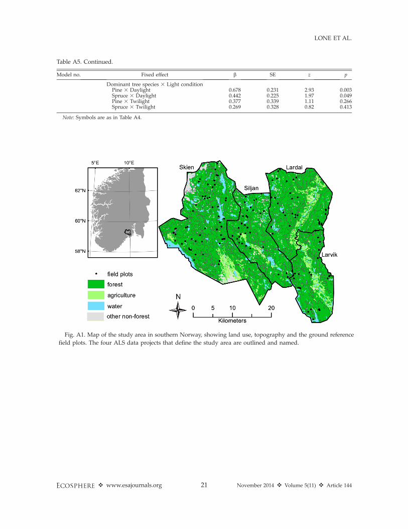
Fig. A1. Map of the study area in southern Norway, showing land use, topography and the ground reference

field plots. The four ALS data projects that define the study area are outlined and named.

Table A5. Continued.


Dominant tree species 3 Light conditionPine 3 Daylight 0.678 0.231 2.93 0.003Spruce 3 Daylight 0.442 0.225 1.97 0.049Pine 3 Twilight 0.377 0.339 1.11 0.266Spruce 3 Twilight 0.269 0.328 0.82 0.413

Note: Symbols are as in Table A4.


LONE ET AL.

Fig. A2. K-fold (k¼ 5) cross-validation plots for the best forage biomass models based on forest inventory data

(inv), ALS data (ALS), or forest inventory and ALS data (invþALS). Modeled browse categories are (A, B, C)

RAW winter, (D, E, F) RAW summer, (G, H, I) pine winter, (J, K, L) total biomass winter, and (M, N, O) total

biomass summer. Two trend lines are shown: the ideal 1:1 relationship (black) and the least-squares trend line

(red) between predicted and field measured values. The original biomass data were in g/m2.


LONE ET AL.

improving broad scale forage mapping and habitat selection...

Documents