improving delivery efficiency and effectiveness for the ... · improving delivery efficiency and...

Improving Delivery Efficiency and Effectiveness for the

DRINK-MË App

A Major Qualifying Project Report submitted to the Faculty of

Worcester Polytechnic Institute

In partial fulfillment of the requirements for the Degree of Bachelor of Science

March 24, 2016

Submitted By

Yi Yang

Advisor

Sharon A. Johnson

i

Abstract

The DRINKMË-App, founded by Destination Chengdu Technology LLC and launched

in 2015, is a wine portal that provides customers with an unparalleled immediate delivery

service. The company faced challenges delivering orders in their new market Shanghai due to a

larger coverage area and higher delivery costs. The goal was to improve the logistics system by

(1) completing a pilot study to test potential improvements in operations, (2) creating an Arena

model to analyze alternatives. A mixed-transportation delivery approach was recommended.

ii

Executive Summary

The DRINKMË-App, founded by Destination Technology LLC and launched in 2015 in

Chengdu, is an online wine portal that is committed to providing the highest levels of customer

service through an unparalleled immediate delivery service. The DRINK team aims to bring an

authentic wine experience to customers, in their home, through an exclusive online selection of

beers, wines and other types of liquors. The DRINK team offers an easy-to-use, online-only

service to bring consumers an expanding selection of wines from highly rated vineyards around

the world at maximum convenience.

However, because the market scale in their new market Shanghai is much larger, the

DRINK team encountered issues delivering orders efficiently. Because Shanghai is much larger

and more densely populated than Chengdu, a faster delivery process could improve customer

satisfaction.

The goal of our project was to develop a more efficient delivery process for the

DRINKMË-App. Such an improvement is expected to result in better customer ratings, and then

improve the marketability. The project objectives were to:

1. Assess Current Logistics Performance

2. Arrange a Pilot Study to Explore Potential Alternatives

3. Develop a Simulation Model

4. Experiment with the Simulation to Explore Alternatives

The result of the project is a recommendation about how to create an efficient system that

can facilitate DRINKMË team’s operations in the long run. From the pilot study, we found that

choosing a mixed transportation delivery method including both cars and bikes achieves a

solution that balances both financial and delivery time goals. Also, by developing a simulation

model, the team explored 11 scenarios. Based on sensitivity analysis, two best scenarios

emerged. One alternative, which came from the pilot study suggests, a resource configuration

with 6 bikes, 2 cars and 3 administrators. The second came from the simulation analysis,

including 4 bikes, 4 cars and 1 administrators. As a result of this project, the team recommended

the solution from the simulation because it includes only 9 resources instead of the 11 in the

original scenario, which is more efficient. In addition, improvements such as revising the back-

office system and database system are also recommended to the DRINKMË team to facilitate

their overall long-run operation.

iii

Acknowledgments I would like to thank the DRINKMË management team and the back-stage interface team,

along with finance department, for providing the opportunity to complete a project.

I would also like to thank Sharon Johnson, the advisor of this project, for being a great

supporter for me and this project.

iv

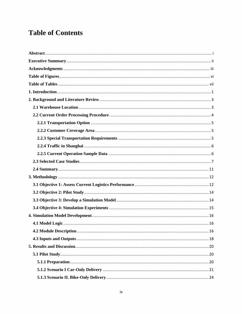
Table of Contents

Abstract ......................................................................................................................................................... i

Executive Summary .................................................................................................................................... ii

Acknowledgments ...................................................................................................................................... iii

Table of Figures.......................................................................................................................................... vi

Table of Tables .......................................................................................................................................... vii

1. Introduction ............................................................................................................................................. 1

2. Background and Literature Review ...................................................................................................... 3

2.1 Warehouse Location ......................................................................................................................... 3

2.2 Current Order Processing Procedure ............................................................................................. 4

2.2.1 Transportation Option .............................................................................................................. 5

2.2.2 Customer Coverage Area .......................................................................................................... 5

2.2.3 Special Transportation Requirements ..................................................................................... 5

2.2.4 Traffic in Shanghai .................................................................................................................... 6

2.2.5 Current Operation Sample Data .............................................................................................. 6

2.3 Selected Case Studies ........................................................................................................................ 7

2.4 Summary .......................................................................................................................................... 11

3. Methodology .......................................................................................................................................... 12

3.1 Objective 1: Assess Current Logistics Performance .................................................................... 12

3.2 Objective 2: Pilot Study .................................................................................................................. 14

3.3 Objective 3: Develop a Simulation Model ..................................................................................... 14

3.4 Objective 4: Simulation Experiments ........................................................................................... 15

4. Simulation Model Development ........................................................................................................... 16

4.1 Model Logic ..................................................................................................................................... 16

4.2 Module Description ......................................................................................................................... 16

4.3 Inputs and Outputs ......................................................................................................................... 18

5. Results and Discussion .......................................................................................................................... 20

5.1 Pilot Study........................................................................................................................................ 20

5.1.1 Preparation ............................................................................................................................... 20

5.1.2 Scenario I Car-Only Delivery ................................................................................................. 21

5.1.3 Scenario II. Bike-Only Delivery .............................................................................................. 24

v

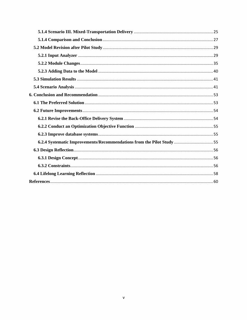
5.1.4 Scenario III. Mixed-Transportation Delivery ....................................................................... 25

5.1.4 Comparison and Conclusion ................................................................................................... 27

5.2 Model Revision after Pilot Study ................................................................................................... 29

5.2.1 Input Analyzer ......................................................................................................................... 29

5.2.2 Module Changes ....................................................................................................................... 35

5.2.3 Adding Data to the Model ....................................................................................................... 40

5.3 Simulation Results .......................................................................................................................... 41

5.4 Scenario Analysis ............................................................................................................................ 41

6. Conclusion and Recommendation ....................................................................................................... 53

6.1 The Preferred Solution ................................................................................................................... 53

6.2 Future Improvements ..................................................................................................................... 54

6.2.1 Revise the Back-Office Delivery System ................................................................................ 54

6.2.2 Conduct an Optimization Objective Function ...................................................................... 55

6.2.3 Improve database systems ....................................................................................................... 55

6.2.4 Systematic Improvements/Recommendations from the Pilot Study ................................... 55

6.3 Design Reflection ............................................................................................................................. 56

6.3.1 Design Concept ......................................................................................................................... 56

6.3.2 Constraints ................................................................................................................................ 56

6.4 Lifelong Learning Reflection ......................................................................................................... 58

References .................................................................................................................................................. 60

vi

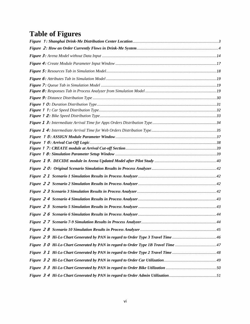
Table of Figures Figure １: Shanghai Drink-Me Distribution Center Location ................................................................................... 3

Figure ２: How an Order Currently Flows in Drink-Me System ............................................................................... 4

Figure３: Arena Model without Data Input ............................................................................................................... 14

Figure４: Create Module Parameter Input Window .................................................................................................. 17

Figure５: Resources Tab in Simulation Model ........................................................................................................... 18

Figure６: Attributes Tab in Simulation Model ........................................................................................................... 19

Figure７: Queue Tab in Simulation Model ................................................................................................................ 19

Figure８: Responses Tab in Process Analyzer from Simulation Model ..................................................................... 19

Figure９: Distance Distribution Type ........................................................................................................................ 30

Figure１０: Duration Distribution Type .................................................................................................................... 31

Figure１１: Car Speed Distribution Type .................................................................................................................. 32

Figure１２: Bike Speed Distribution Type ................................................................................................................. 33

Figure１３: Intermediate Arrival Time for Apps Orders Distribution Type .............................................................. 34

Figure１４: Intermediate Arrival Time for Web Orders Distribution Type ............................................................... 35

Figure １５: ASSIGN Module Parameter Window .................................................................................................. 37

Figure １６: Arrival Cut-Off Logic ........................................................................................................................... 38

Figure１７: CREATE module at Arrival Cut-off Section ........................................................................................ 39

Figure１８: Simulation Parameter Setup Window .................................................................................................. 39

Figure １９. DECIDE module in Arena Updated Model after Pilot Study ............................................................ 40

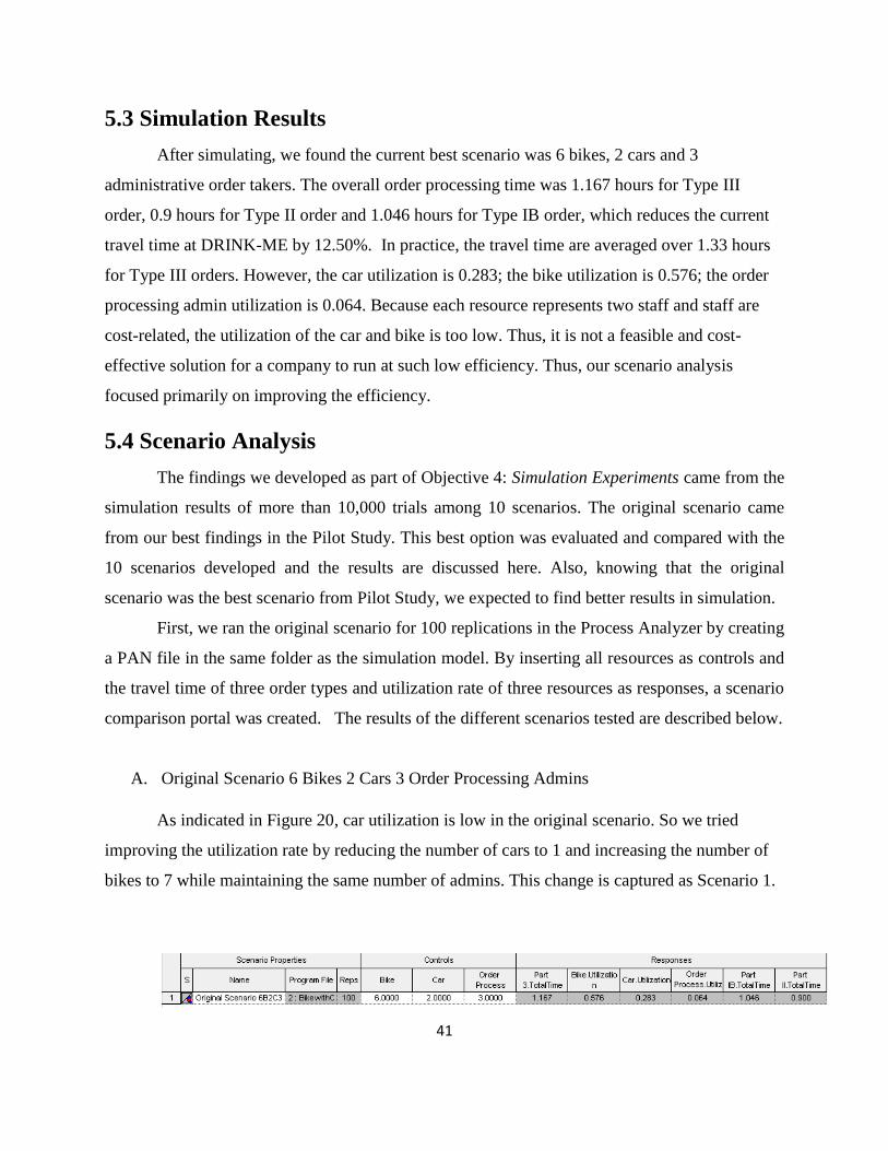
Figure ２０: Original Scenario Simulation Results in Process Analyzer ............................................................... 42

Figure ２１ Scenario 1 Simulation Results in Process Analyzer ............................................................................ 42

Figure ２２ Scenario 2 Simulation Results in Process Analyzer ............................................................................ 42

Figure ２３ Scenario 3 Simulation Results in Process Analyzer ............................................................................. 42

Figure ２４ Scenario 4 Simulation Results in Process Analyzer ............................................................................ 43

Figure ２５ Scenario 5 Simulation Results in Process Analyzer ............................................................................ 43

Figure ２６ Scenario 6 Simulation Results in Process Analyzer ............................................................................ 44

Figure ２７ Scenario 7-9 Simulation Results in Process Analyzer ......................................................................... 44

Figure ２８ Scenario 10 Simulation Results in Process Analyzer .......................................................................... 45

Figure ２９ Hi-Lo Chart Generated by PAN in regard to Order Type 3 Travel Time ........................................... 46

Figure ３０ Hi-Lo Chart Generated by PAN in regard to Order Type 1B Travel Time ........................................ 47

Figure ３１ Hi-Lo Chart Generated by PAN in regard to Order Type 2 Travel Time ........................................... 48

Figure ３２ Hi-Lo Chart Generated by PAN in regard to Order Car Utilization................................................... 49

Figure ３３ Hi-Lo Chart Generated by PAN in regard to Order Bike Utilization ................................................. 50

Figure ３４ Hi-Lo Chart Generated by PAN in regard to Order Admin Utilization .............................................. 51

vii

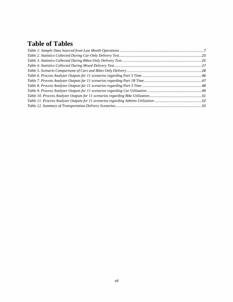
Table of Tables Table 1: Sample Data Sourced from Last Month Operations ....................................................................................... 7 Table 2. Statistics Collected During Car-Only Delivery Test...................................................................................... 23 Table 3. Statistics Collected During Bikes-Only Delivery Test ................................................................................... 25 Table 4. Statistics Collected During Mixed Delivery Test ........................................................................................... 27 Table 5. Scenario Comparisons of Cars and Bikes Only Delivery .............................................................................. 28 Table 6. Process Analyzer Outputs for 11 scenarios regarding Part 3 Time .............................................................. 46 Table 7. Process Analyzer Outputs for 11 scenarios regarding Part 1B Time ............................................................ 47 Table 8. Process Analyzer Outputs for 11 scenarios regarding Part 3 Time .............................................................. 48 Table 9. Process Analyzer Outputs for 11 scenarios regarding Car Utilization ......................................................... 49 Table 10. Process Analyzer Outputs for 11 scenarios regarding Bike Utilization ...................................................... 51 Table 11. Process Analyzer Outputs for 11 scenarios regarding Admins Utilization ................................................. 52 Table 12. Summary of Transportation Delivery Scenarios .......................................................................................... 53

1

1. Introduction

Destination (Chengdu) Technology LLC, founded in late 2014 in Chengdu, Sichuan, was

excited to launch its online portal, DRINKMË-App on May 28, 2015. DRINKMË-App is an

online wine portal that is committed to providing the highest levels of convenience, elegance and

hospitality for the customers. The DRINK team aims to bring the authentic wine experience to

customers, in their home, through our unparalleled online selection of beers, wines and other

types of liquors("DRINKMË, Your Private Butler" n.d.).

The DRINK team does not agree with the accepted notion that the world of wine should

be exclusive, snooty or expensive. This is why the DRINK team offers an easy-to-use, online-

only service to bring consumers the expanding selection of wines from highly rated-vineyards

around the world at maximum convenience. The DRINKMË-App is designed to be easy to use,

involving just one click to sign in and order, and wine will be delivered to the customers at the

push of a button.

Destination (Chengdu) Technology LLC is in the business of hospitality, and throughout

the convenient process, customers have access to the warmth of a human instead of a machine.

The DRINKMË-App provides immediate contact by phone and an instant notification to confirm

that delivery is on the way. Also, the DRINK team uses data analysis and dynamic algorithms to

recognize customers’ preferences and invite them to suitable wine tastings and join the wine

club. Unlike traditional e-commerce with slow logistics, a crucial feature of DRINKMË is the

delivery speed, which is 20-40 minutes inside the Inner Ring Area of both Shanghai and

Chengdu, and within 60 minutes outside the cities.

Within 3 months after the launch of the innovative product, the number of customers

exceeded 10,000 and the company was able to raise $0.4 million venture capital in the latest

round of financing. However, because the market scale in Chengdu is not the largest in China, all

wine delivery is on a purchase basis. Thus, operations in Chengdu are like a logistics company

with wine. With a smaller scale market and a more concentrated selections of wines, the DRINK

team is able to delivery alcohol from the warehouse within 20-40 minutes after receiving the

orders. Currently, the DRINK team is expanding the service in major Shanghai areas.

2

The DRINKMË APP team has encountered several challenges associated with delivering

wines efficiently in their new market of Shanghai. The DRINK team would like to achieve

maximum the delivery rate at the least cost. Since Shanghai is much larger and more densely

populated than Chengdu, currently, if the orders contain goods from both the Distribution Center

and third-party stores, the delivery rate will be slower and cost will be much higher. Also, a

faster delivery process could improve customer satisfaction. However, faster delivery requires

extra cost. The most economical way for delivery team to achieve fastest delivery is the ultimate

goal. Also, it would be a bonus if marketing process could be combined into delivery process,

which will make the operations of the whole delivery team more efficient.

The goal of our project was to develop a more efficient delivery process for DRINKMË-

App. Such an improvement is expected to allow DRINKMË to earn better customer ratings, and

then improve marketability. To achieve this improvement to the system, the team pursued the

following objectives:

1. Assess current logistics system performance

2. Complete a pilot study to explore potential alternatives

3. Develop a simulation model

4. Experiment with the simulation to explore alternatives.

Completing these objectives contributed to providing a potential solution to DRINKMË.

3

2. Background and Literature Review

The purpose of this chapter is to provide a deeper understanding of the background

information necessary to support the project goals and objectives. This section describes the

warehouse of the DRINKMË system, including data from recent operations, current delivery

modes and types of orders. The chapter also explores best practices for the use of Arena

Rockwell Software to facilitate last-mile deliver by reviewing similar cases. Finally, several case

studies are examined to learn how to approach similar scenes in logistics industry.

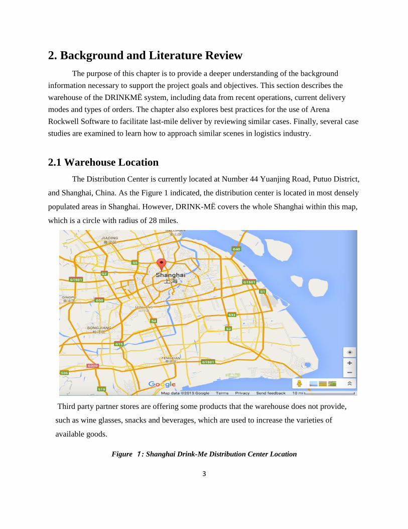
2.1 Warehouse Location

The Distribution Center is currently located at Number 44 Yuanjing Road, Putuo District,

and Shanghai, China. As the Figure 1 indicated, the distribution center is located in most densely

populated areas in Shanghai. However, DRINK-MË covers the whole Shanghai within this map,

which is a circle with radius of 28 miles.

Third party partner stores are offering some products that the warehouse does not provide,

such as wine glasses, snacks and beverages, which are used to increase the varieties of

available goods.

Figure １: Shanghai Drink-Me Distribution Center Location

4

2.2 Current Order Processing Procedure

Currently, DRINK-MË processes these types of orders, including type 1 orders which

only contain warehouse products, type 2 orders that only accommodates third-party products,

and type 3 orders which contain both warehouse and their-party products. The order processing

procedure is shown in Figure 2.

Figure ２: How an Order Currently Flows in Drink-Me System

As Figure 2 indicates, the standard operating procedure shows that orders containing only goods

from warehouse, are processed from the distribution center (DC) and delivered, the fastest. Then,

3rd party only orders are delivered by 3rd party logistics upon request of the 3rd party stores.

Last, the orders containing both warehouse products and 3rd

party products are handled by first

5

picking up from the DC and then picking up the goods from 3rd

party stores. Apparently, type 3

orders took the longest time to deliver.

2.2.1 Transportation Option

There are three types of transportation available in the wine delivery process as discussed

below.

Cars - Expensive, slow during peak hours but can carry a lot of products at the same time,

costs 1.3$/km + 14$/hour labor overhead, can handle multiple orders with one roundtrip.

Normally take 20-40 minutes to deliver.

Electronic Bikes – Inexpensive option, average speed regardless of traffic condition but

can ONLY carry just 6 bottles at maximum, costs 0.2$/km+ 6$/hour labor overhead, can

only handle 1-2 orders maximum. Normally take 30-60 minutes to deliver.

Third-Party Logistics Company -the most expensive transportation, using motorbikes or

public transportation like subway to avoid traffic, with the same carrying capacity as

Electronic Bikes, costs nearly 1$/km without any extra costs.

Normally, if an order contains 3rd party goods only, it can only be delivered by a 3rd party

logistics as there is no extra human labor costs.

2.2.2 Customer Coverage Area

Shanghai, a circular area with a radius of 28 miles, covers a total amount of 5 million

potential customers with an existing base of 9000 users.

2.2.3 Special Transportation Requirements

Several types of alcohols require extra special equipment or instruments to deliver,

regardless of costs, in the industry:

6

Champagne - Champagnes cannot be transported by electronic bikes due to the

vulnerability of sparkling wines inside, which can explode dangerously while being

opened.

Beer - Beer orders normally have low profit margin; however, they require the most

capable carriers since they have high volume. Thus, looking for the cheapest

transportation method, such as motorbikes, is the key option.

Third-Party Goods - All third-party goods, if ordered separated from goods in the

Distribution Center, will be delivered by third-party logistics. However, if mixed

Distribution Center products, the situation is more complex. The delivery person from

DRINKMË will pick up items from the Distribution Center and then transport them to

third-party stores regardless of distances. Finally the order will be sent to the clients by

the delivery person from DRINKMË.

2.2.4 Traffic in Shanghai There are peak hours in the morning and evening times. However, different traffic

limitations code will restrain usage of the delivery truck. In peak hours, it is the most efficient to

use electronic bikes to deliver. The current rush hour in Shanghai, according to data from

People’s Public of China’s Traffic Administration Department, is roughly from 5pm to 8pm.

Also, China is employing a limitation on use of cars by only allowing cars with odd plate number

to travel on Monday, Wednesday, Friday and Sunday. Otherwise, only cars with even plate

number are allowed to travel.

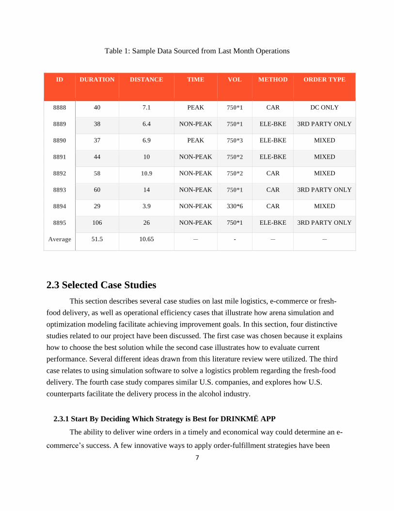
2.2.5 Current Operation Sample Data Sample data from current operation is shown in Table 1. The first column represents the

order number. Information is also available about the time the orders took, the distance, the

method of transportation and type of order.

7

Table 1: Sample Data Sourced from Last Month Operations

ID DURATION DISTANCE TIME VOL

METHOD ORDER TYPE

8888 40 7.1 PEAK 750*1 CAR DC ONLY

8889 38 6.4 NON-PEAK 750*1 ELE-BKE 3RD PARTY ONLY

8890 37 6.9 PEAK 750*3 ELE-BKE MIXED

8891 44 10 NON-PEAK 750*2 ELE-BKE MIXED

8892 58 10.9 NON-PEAK 750*2 CAR MIXED

8893 60 14 NON-PEAK 750*1 CAR 3RD PARTY ONLY

8894 29 3.9 NON-PEAK 330*6 CAR MIXED

8895 106 26 NON-PEAK 750*1 ELE-BKE 3RD PARTY ONLY

Average 51.5 10.65 － - －－

2.3 Selected Case Studies

This section describes several case studies on last mile logistics, e-commerce or fresh-

food delivery, as well as operational efficiency cases that illustrate how arena simulation and

optimization modeling facilitate achieving improvement goals. In this section, four distinctive

studies related to our project have been discussed. The first case was chosen because it explains

how to choose the best solution while the second case illustrates how to evaluate current

performance. Several different ideas drawn from this literature review were utilized. The third

case relates to using simulation software to solve a logistics problem regarding the fresh-food

delivery. The fourth case study compares similar U.S. companies, and explores how U.S.

counterparts facilitate the delivery process in the alcohol industry.

2.3.1 Start By Deciding Which Strategy is Best for DRINKMË APP

The ability to deliver wine orders in a timely and economical way could determine an e-

commerce’s success. A few innovative ways to apply order-fulfillment strategies have been

8

created by Lee in his 2001 study regarding the importance of last-mile delivery, which primarily

involve making good use of information and leveraging existing resources to coordinate order-

fulfillment activities. The core strategies that DRINKMË could use: dematerialization, referring

to the maximum use of information, and resource exchange, and the clicks-and-mortar model.

First, DRINKMË should understand the product characteristics. To understand what strategy

might be the best, the following should be considered.

• Where the customers and what are the delivery-value densities?

• What level of demand uncertainty exists for the product?

• What fraction of products can be dematerialized?

For DRINKMË, customers are in need of fast delivery along with reasonable price. They

are densely populated among 6 to 8 miles of radius in central Shanghai. There is seasonality with

this product: high demand in summer and winter break along with 40% lower demand on usual

business days. Delivery process notifications, signature and reconfirmation panel can be

dematerialized.

Second, it is necessary for DRINKMË to understand the environment and excellent performance.

• Are there reliable information-intensive logistics-service providers?

• How is the current system rated?

There are several data share systems built in current mobile apps. Before going forward

with the project, the DRINKMË team should familiar themselves with how current system

performs based on a few key components such as time-efficiency, cost-effectiveness, risk and

customer service ratings.

Third, DRINKMË need to formulate the options.

• Use as much resource exchange as possible.

• Use information to coordinate the deliveries intelligently.

• Assess the options.

• Explore synergies between online and offline order fulfillment.

There are synergies between online and offline system. It is important to consider cost,

efficiency, reliability and risks to identify additional values and services that could be offered to

DRINKMË customers. In additional to DRINKMË’s own system, it would be wise to consider

9

the links between existing infrastructures and other partnerships to exchange the resource,

creating a win-win cost effective logistics mode.

2.3.2 Measure Current Performance

In addition to developing strategies, it is important to measure the performance of a

logistics system (Mentzer et al 1991). The evaluation of logistics is divided into three areas:

productivity, utilization, and performance, where productivity is the ratio of real output to real

input, utilization is the ratio of capacity used to available capacity, and performance is the ratio

of actual output to standard output. Performance measurement is an analysis of both

effectiveness and efficiency in accomplishing a given task such as alcohol delivery. Second,

establishing goals based on current performance are necessary. However, the logistics goals may

be conflicted with the marketing goals. Effectiveness is defined as the extent to which goals are

accomplished. Efficiency is the measure of how well the resources expended are utilized.

DRINKMË, identified as a “Stage I” companies, or “inactive companies”, will need to

use very simple measures that are expressed in terms of dollars (Mentzer et al 1991). The

information regarding current logistics performance usually comes from financial department

and a few other ratios based on operations. However, the standardized procedure for logistics

performance assessment could not be applied in this situation. In order for the DRINK team to

implement those strategies, DRINKMË needs to develop a simple and easy-to-use assessment

standard to rate the current logistics performance, which is suggested to be delivery speed

(km/h), average costs ($) and average unit cost (costs per kilometer) ($/km) using three types of

transportation methods. In addition to these efficiency attributes, customer ratings are also

considered as customer satisfaction indexes. Additionally, in order to evaluate the overall

balance between efficiency and customer ratings, we assign customer ratings divided by unit cost

as an accumulated overall performance value, which means, the larger the results, the better the

operations.

Third, delivery speed, cost controls, and customer service are all impacted by availability.

Availability can be accomplished through better information to manage product flows and reduce

inventory. Benefits are further enhanced by greater collaboration between supply chain partners

to increase speed and flexibility, and the ability to create entirely new supply chains operations.

10

Thus, by sharing data with supply chain partners to the DRINK team will be able to provide the

information needed to be successful in supply chain management.

2.3.3 Use of Modeling and Simulation (M&S)

Modeling and simulation (M&S) is an important tool when applied to on-demand

logistics industries such as fresh food or wine delivery companies such as DRINKMË (Arena

Simulation, n.d.). Arena, by Rockwell Software could run a logistics simulation model to

evaluate changes to existing delivery systems before implementing them in the actual operations.

Arena modeling can be used to help understand the impact of changes the team proposed to

make on in the DRINKMË operations, to determine costs associated with alternative approaches

and to provide a what-if analysis tool to evaluate future enhancements to process.

Also, it is evident that wine and beverage delivery could be very similar to the fresh-food

supply chain, which represents a very interesting application area, considering all the inter-

related constraints and variables: time-to-market, traceability, transport/storage conditions,

handling, production/process control, demand variability, and seasonal behaviors. In order to

increase margins on specific products such as 3rd party foods and alcoholic products, an

effective modeling of the system regarding the logistics operation costs and inventory control is

needed in order to develop new solutions for these special supply chain delivery. This modeling

approach requires development of simulation models in order to achieve different results such as

faster wine-delivery processes and rapid response with cost control.

Finally, developing an optimization model in Excel could help find the theoretically best

solutions from different scenarios simulated in Arena models. By utilizing both Excel and Arena,

the company would be able to not only simulate the material flow such as vehicle routing,

employee scheduling, and order flows but also information flows problems. From warehouse to

final customers, the flow of bottles is processed and moved along the different phases of the

supply chain, while in the opposite direction information flows are used for driving the planning

and distribution. The company could use the solver to create a logistics model with changing

cells to test the design using customized constraints before making real changes.Thus,

DRINKMË is able to find the new way to delivery under the least costs and risks.

11

2.3.4 Benchmark Drizly or Saucey’s Alcohol Delivery System

Companies can often find ideas for improvement by benchmarking against other

competitors. Boston-based Drizly is trying to innovate in the wine industry with fast delivery.

While the typical startup founder rhapsodizes about big data algorithms, Rellas, co-founder of

Drizly, calls Drizly “just a fax machine.” Drizly routes the order to a retail partner able to deliver

in 20 to 40 minutes (Soper 2014). Drizly uses the employees from the liquor store to deliver

instead of delivering them on their own. However, as long as the cost of delivery is based on

percentage of revenues by bottle, the delivery range could be limited. As for DRINKMË APP,

which provides the very similar service, it could be considered to cut all delivery team and

transportation costs by transferring them to part of revenues obtained from third-party stores. Los

Angeles-based Saucey is another industry legend in delivering alcohols. The Saucey App

designed a request-basis system registered by free drivers. The way Saucey delivery alcohols is

basically gather all free and unemployed drivers to maximize the profits by not contracting any

regular delivery team. However, as for DRINKMË, it is not wise to choose the option right now

since Saucey system requires significantly more technology costs under current circumstances.

2.4 Summary

In the process of exploring the nature of last-mile logistics, arena simulation and

efficiency of logistics, we were able to make use of our knowledge from the study of Industrial

Engineering related to the DRINK team’s challenges. Our review of the literature revealed

several key points: first, current logistics performance need to be evaluated regardless of

company size; second, all improvements should be based on current performance; third, to

perform a real operation is a good way to find the current bottleneck in the system; fourth, by

using simulation software such as Arena Rockwell, better solution at a lowest cost can be found;

fifth, building proper model might be the most important task within this project. We also

evaluated the alcohol delivery processes of other organizations or competitors. This researches

and studies provided valuable insight into how to achieve objectives.

12

3. Methodology

The goal of this project was to improve the DRINKMË logistics system by evaluating

current performance and exploring potential improvements. To meet this goal, our objectives and

a brief description of our methods are presented here:

1. Assess Current Logistics Performance

a. Evaluate current performance based on historical database

b. Create customized logistics ratings

2. Pilot Study

a. Establish potential assumptions

b. Mini-test potential assumptions in real operations

3. Develop a Simulation Model

a. Design an Arena model

b. Validate the model

4. Simulation Experiments

a. Simulate Different Alternatives

b. Use Process Analyzer to produce the best options by comparing scenarios

These objectives and methodologies are described in more detailed below.

3.1 Objective 1: Assess Current Logistics Performance

In order to evaluate current logistics performance, the company should be able to

characterize its current stage. As Logistics Performance Ratings indicated, DRINKMË is listed

as “Stage I” based on current number of orders and users. Thus, there is no fixed standard for this

situation. Instead, the team would like to use delivery speed (km/h), average costs and average

unit costs (costs per kilometer) to evaluate the efficiency of the system. The equations are

outlined as follows:

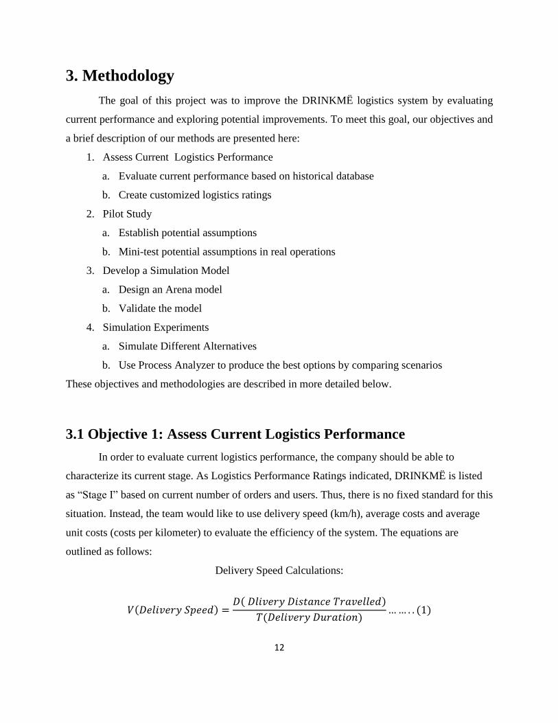
Delivery Speed Calculations:

𝑉(𝐷𝑒𝑙𝑖𝑣𝑒𝑟𝑦 𝑆𝑝𝑒𝑒𝑑) =𝐷( 𝐷𝑙𝑖𝑣𝑒𝑟𝑦 𝐷𝑖𝑠𝑡𝑎𝑛𝑐𝑒 𝑇𝑟𝑎𝑣𝑒𝑙𝑙𝑒𝑑)

𝑇(𝐷𝑒𝑙𝑖𝑣𝑒𝑟𝑦 𝐷𝑢𝑟𝑎𝑡𝑖𝑜𝑛)… … . . (1)

13

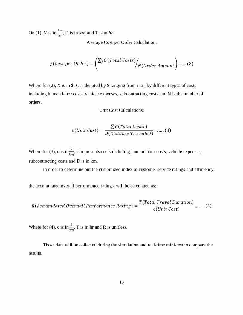
On (1). V is in 𝑘𝑚

ℎ𝑟, D is in 𝑘𝑚 and T is in ℎ𝑟

Average Cost per Order Calculation:

𝜒(𝐶𝑜𝑠𝑡 𝑝𝑒𝑟 𝑂𝑟𝑑𝑒𝑟) = (∑ 𝐶𝑖

𝑗 (𝑇𝑜𝑡𝑎𝑙 𝐶𝑜𝑠𝑡𝑠)𝑁(𝑂𝑟𝑑𝑒𝑟 𝐴𝑚𝑜𝑢𝑛𝑡

⁄ ) … … (2)

Where for (2), X is in $, C is denoted by $ ranging from i to j by different types of costs

including human labor costs, vehicle expenses, subcontracting costs and N is the number of

orders.

Unit Cost Calculations:

𝑐(𝑈𝑛𝑖𝑡 𝐶𝑜𝑠𝑡) =∑ 𝐶(𝑇𝑜𝑡𝑎𝑙 𝐶𝑜𝑠𝑡𝑠 )

𝐷(𝐷𝑖𝑠𝑡𝑎𝑛𝑐𝑒 𝑇𝑟𝑎𝑣𝑒𝑙𝑙𝑒𝑑)… … . (3)

Where for (3), c is in$

𝑘𝑚, C represents costs including human labor costs, vehicle expenses,

subcontracting costs and D is in km.

In order to determine out the customized index of customer service ratings and efficiency,

the accumulated overall performance ratings, will be calculated as:

𝑅(𝐴𝑐𝑐𝑢𝑚𝑢𝑙𝑎𝑡𝑒𝑑 𝑂𝑣𝑒𝑟𝑎𝑎𝑙𝑙 𝑃𝑒𝑟𝑓𝑜𝑟𝑚𝑎𝑛𝑐𝑒 𝑅𝑎𝑡𝑖𝑛𝑔) =𝑇(𝑇𝑜𝑡𝑎𝑙 𝑇𝑟𝑎𝑣𝑒𝑙 𝐷𝑢𝑟𝑎𝑡𝑖𝑜𝑛)

𝑐(𝑈𝑛𝑖𝑡 𝐶𝑜𝑠𝑡)… … . (4)


𝑘𝑚, T is in hr and R is unitless.

Those data will be collected during the simulation and real-time mini-test to compare the

results.

14

3.2 Objective 2: Pilot Study

Based on the background knowledge of sponsoring agency, we decided to do a 'soft'

research, conducting a preliminary analysis before committing to a full-blown study or

experiment. In pilot study, we are going to test the assumption of potential alternatives. It is

assumed that either car-only delivery or bike-only delivery would be more efficient. Also,

another combined transportation method is very popular in food delivery industry of China. The

pilot study is going to evaluate those options based on mini-run and collect data to find out if the

total travel time or cost is more efficient.

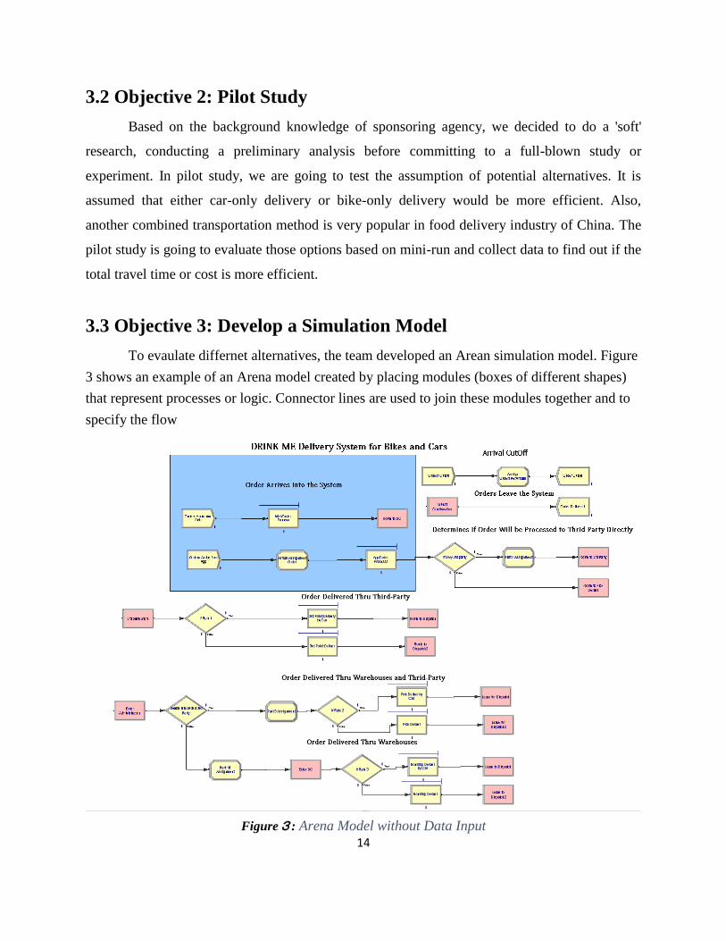
3.3 Objective 3: Develop a Simulation Model

To evaulate differnet alternatives, the team developed an Arean simulation model. Figure

3 shows an example of an Arena model created by placing modules (boxes of different shapes)

that represent processes or logic. Connector lines are used to join these modules together and to

specify the flow

Figure３: Arena Model without Data Input

15

of entities. Statistical data, such as lead time, cost and other real-time data point, can be recorded

and outputted as reports. Arena can be integrated with Microsoft technologies, including

Microsoft Visio flowcharts, as well as Excel spreadsheets and Access databases. In this case,

Arena can simulate multiple operation types, including wine from distribution center to final

customer, for optimizing the efficiency of working shift and delivery vehicles, reducing the

overall waiting time for customers and reducing the overall costs for the company.

3.4 Objective 4: Simulation Experiments

We proposed to simulate the model more than 10,000 times simply by changing

controlled resources while keeping the all other variables and attributes constant. By utilizing the

process analyzer in Arena, we are able to find the best solution and tell if the solution is

significant better by confidence intervals with half-width.

16

4. Simulation Model Development

This section describes the simulation model that was developed.

4.1 Model Logic

The Arena model simulates the delivery process of an order from arrival to its dispatch.

There are three main sections in this model: the arrival section, the order processing section and

the disposal section. A diagram of the simulation model is shown in Figure 3. In the arrival

section, there are three order arrival CREATE entities, designed to simulate the three types of

arrivals and two resources: order with reserved time stamp from website, order with or without

reserved time stamp from App. The three different types of arrivals have different distributions,

(uniform or exponential), different assigned attributes, and recorded statistics for outputs. By

using Enter and Leave and Route and Station modules, the model is able to simulate the

transition between procedures with different transfer methods and wait times. This is followed by

a DECIDE module in the order processing section. In the order processing section, it is necessary

to use “Seize”-“Delay”-“Release” to simulate the human resource delivery methods used in the

real time. There are two types of resources in this project, drivers and delivery employees. The

former will drive vehicles for delivery and the later use the motorbike to deliver. After order

processing, all entities in the system end their travel at the disposal station (guest confirmation

station).

4.2 Module Description

Each module is documented more completely in this section.

• Arrival Section

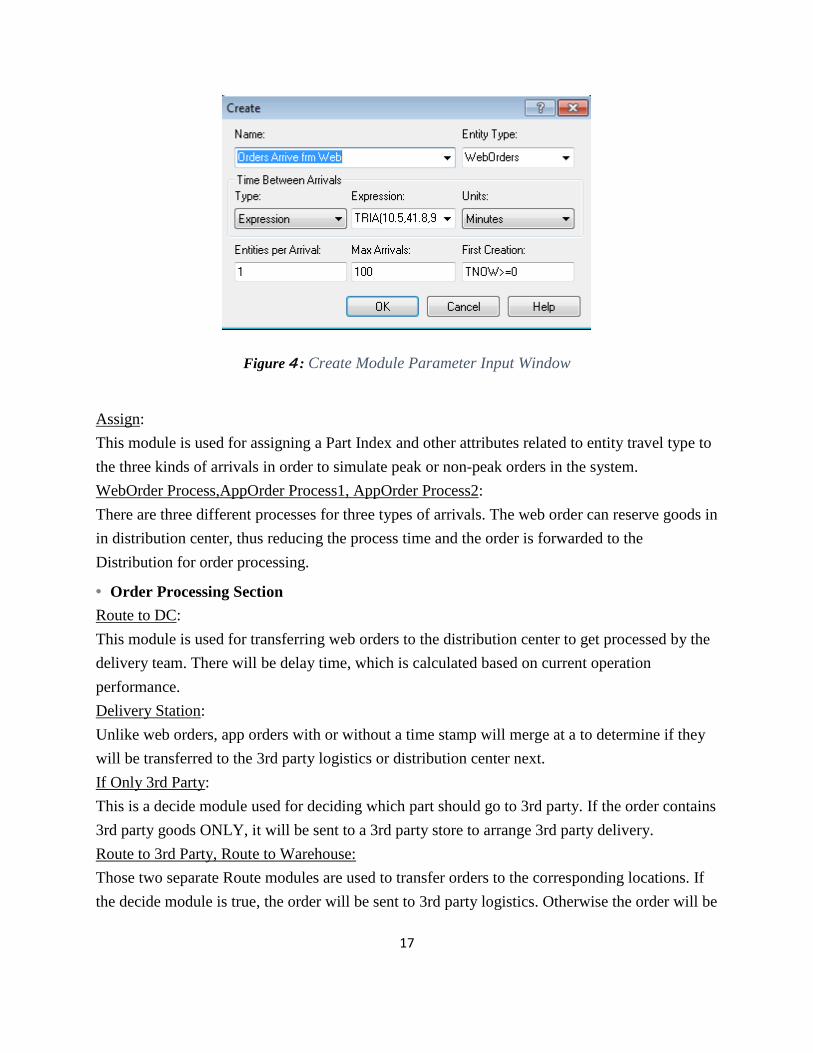
Order arrived from App, Order arrived from Web:

The two types of arrivals from App and Web have different types of distributions, including but

not limited to order size, order volume, and arrival rates. As Figure 4 Indicated, the parameters

used in the CREATE module and the first creation happen at TNOW>=0.

17

Figure４: Create Module Parameter Input Window

Assign:

This module is used for assigning a Part Index and other attributes related to entity travel type to

the three kinds of arrivals in order to simulate peak or non-peak orders in the system.

WebOrder Process,AppOrder Process1, AppOrder Process2:

There are three different processes for three types of arrivals. The web order can reserve goods in

in distribution center, thus reducing the process time and the order is forwarded to the

Distribution for order processing.

• Order Processing Section

Route to DC:

This module is used for transferring web orders to the distribution center to get processed by the

delivery team. There will be delay time, which is calculated based on current operation

performance.

Delivery Station:

Unlike web orders, app orders with or without a time stamp will merge at a to determine if they

will be transferred to the 3rd party logistics or distribution center next.

If Only 3rd Party:

This is a decide module used for deciding which part should go to 3rd party. If the order contains

3rd party goods ONLY, it will be sent to a 3rd party store to arrange 3rd party delivery.

Route to 3rd Party, Route to Warehouse:

Those two separate Route modules are used to transfer orders to the corresponding locations. If

the decide module is true, the order will be sent to 3rd party logistics. Otherwise the order will be

18

sent to distribution center. This is calculated using the current average percentage of the two

categories of orders.

Enter DC,3rd Party Delivery:

Those two separate Enter modules are used to receive orders from the arrival sections.

If Mixed Order:

The order processed to distribution center will be separated because the “false” one will be

delivered directly to the customer while the “true” one will need to go through a pick-up, wait

and get delivered procedure.

Size an Employee, Seize a Driver:

The Seize modules are used to seize the resource (employee or driver) and to use the resource to

proceed to next procedure.

• Disposal Section

Delay Order, Release Employee:

The delay and release modules used are used to release the employee and simulate the transfer

period.

Leave to Guest Confirmation:

By using 3 Leave modules and a merged disposal station, we are able to record how long each

order spent in the system, and evaluate alternative which can be used to improve the system.

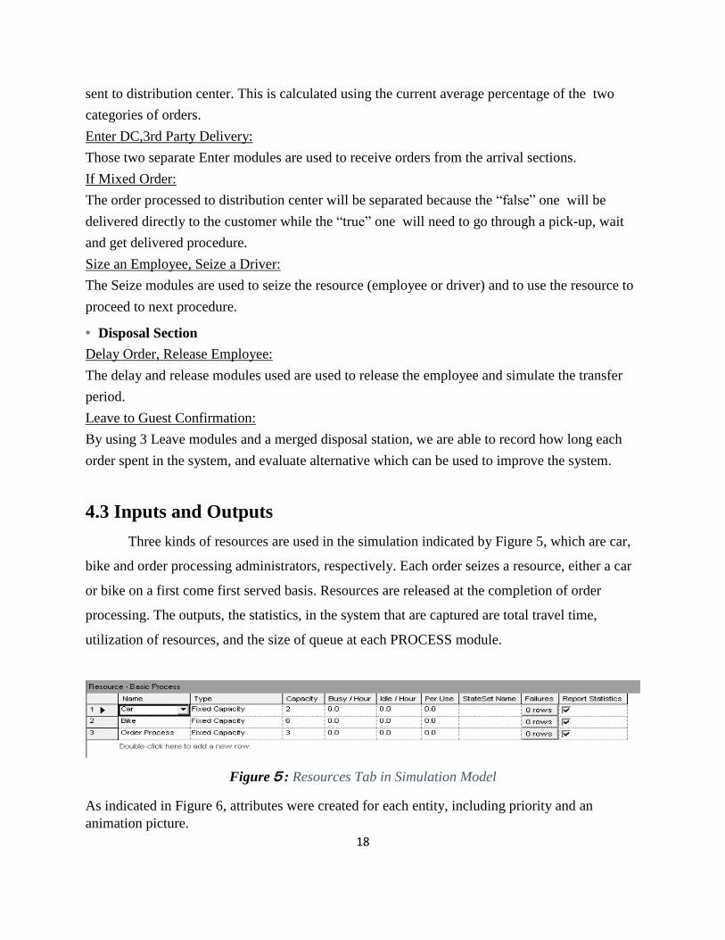
4.3 Inputs and Outputs

Three kinds of resources are used in the simulation indicated by Figure 5, which are car,

bike and order processing administrators, respectively. Each order seizes a resource, either a car

or bike on a first come first served basis. Resources are released at the completion of order

processing. The outputs, the statistics, in the system that are captured are total travel time,

utilization of resources, and the size of queue at each PROCESS module.

Figure５: Resources Tab in Simulation Model

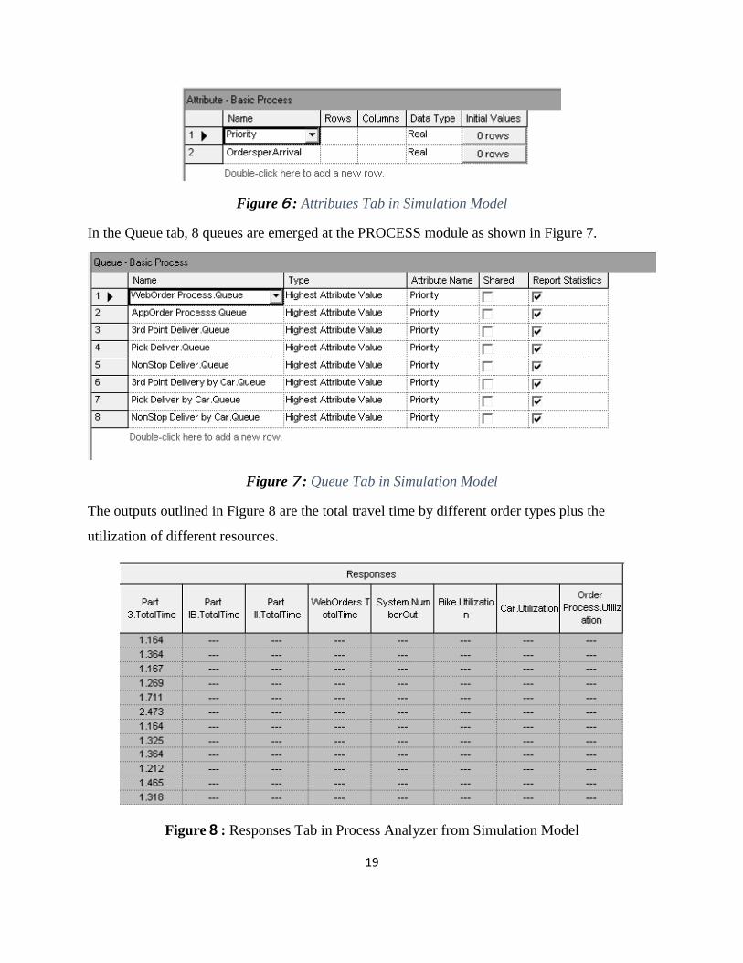
As indicated in Figure 6, attributes were created for each entity, including priority and an

animation picture.

19

Figure６: Attributes Tab in Simulation Model

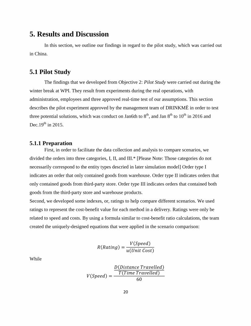
In the Queue tab, 8 queues are emerged at the PROCESS module as shown in Figure 7.

Figure７: Queue Tab in Simulation Model

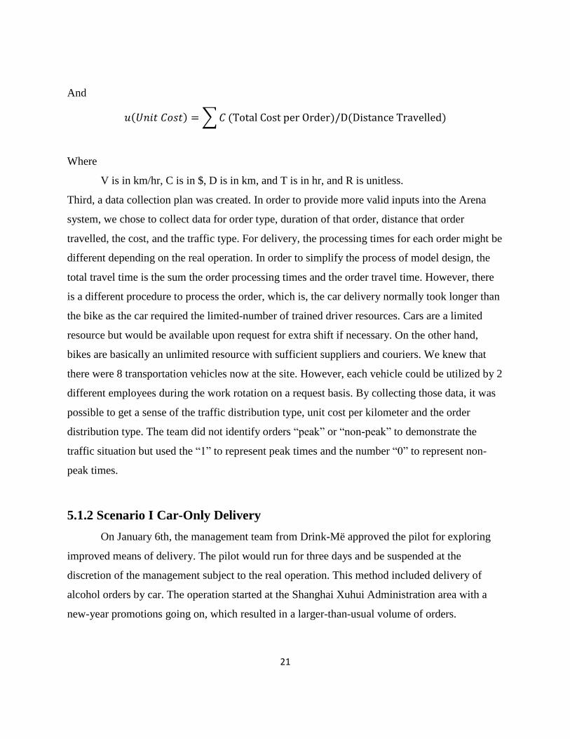
The outputs outlined in Figure 8 are the total travel time by different order types plus the

utilization of different resources.

Figure８: Responses Tab in Process Analyzer from Simulation Model

20

5. Results and Discussion

In this section, we outline our findings in regard to the pilot study, which was carried out

in China.

5.1 Pilot Study

The findings that we developed from Objective 2: Pilot Study were carried out during the

winter break at WPI. They result from experiments during the real operations, with

administration, employees and three approved real-time test of our assumptions. This section

describes the pilot experiment approved by the management team of DRINKMË in order to test

three potential solutions, which was conduct on Jan6th to 8th

, and Jan 8th

to 10th

in 2016 and

Dec.19th

in 2015.

5.1.1 Preparation First, in order to facilitate the data collection and analysis to compare scenarios, we

divided the orders into three categories, I, II, and III.* [Please Note: Those categories do not

necessarily correspond to the entity types descried in later simulation model] Order type I

indicates an order that only contained goods from warehouse. Order type II indicates orders that

only contained goods from third-party store. Order type III indicates orders that contained both

goods from the third-party store and warehouse products.

Second, we developed some indexes, or, ratings to help compare different scenarios. We used

ratings to represent the cost-benefit value for each method in a delivery. Ratings were only be

related to speed and costs. By using a formula similar to cost-benefit ratio calculations, the team

created the uniquely-designed equations that were applied in the scenario comparison:

𝑅(𝑅𝑎𝑡𝑖𝑛𝑔) =𝑉(𝑆𝑝𝑒𝑒𝑑)

𝑢(𝑈𝑛𝑖𝑡 𝐶𝑜𝑠𝑡)

While

𝑉(𝑆𝑝𝑒𝑒𝑑) =

𝐷(𝐷𝑖𝑠𝑡𝑎𝑛𝑐𝑒 𝑇𝑟𝑎𝑣𝑒𝑙𝑙𝑒𝑑)𝑇(𝑇𝑖𝑚𝑒 𝑇𝑟𝑎𝑣𝑒𝑙𝑙𝑒𝑑)

60

21

And

𝑢(𝑈𝑛𝑖𝑡 𝐶𝑜𝑠𝑡) = ∑ 𝐶 (Total Cost per Order)/D(Distance Travelled)

Where

V is in km/hr, C is in $, D is in km, and T is in hr, and R is unitless.

Third, a data collection plan was created. In order to provide more valid inputs into the Arena

system, we chose to collect data for order type, duration of that order, distance that order

travelled, the cost, and the traffic type. For delivery, the processing times for each order might be

different depending on the real operation. In order to simplify the process of model design, the

total travel time is the sum the order processing times and the order travel time. However, there

is a different procedure to process the order, which is, the car delivery normally took longer than

the bike as the car required the limited-number of trained driver resources. Cars are a limited

resource but would be available upon request for extra shift if necessary. On the other hand,

bikes are basically an unlimited resource with sufficient suppliers and couriers. We knew that

there were 8 transportation vehicles now at the site. However, each vehicle could be utilized by 2

different employees during the work rotation on a request basis. By collecting those data, it was

possible to get a sense of the traffic distribution type, unit cost per kilometer and the order

distribution type. The team did not identify orders “peak” or “non-peak” to demonstrate the

traffic situation but used the “1” to represent peak times and the number “0” to represent non-

peak times.

5.1.2 Scenario I Car-Only Delivery

On January 6th, the management team from Drink-Më approved the pilot for exploring

improved means of delivery. The pilot would run for three days and be suspended at the

discretion of the management subject to the real operation. This method included delivery of

alcohol orders by car. The operation started at the Shanghai Xuhui Administration area with a

new-year promotions going on, which resulted in a larger-than-usual volume of orders.

22

In this scenario, all orders, regardless of order type, would be delivered by cars. For type

I and II orders, the system would process the order to either warehouse or third party stores and

the delivery team would pick up the order based on wherever the closest driver was. For type III

orders, the system would first let the car pick up either goods from third party or warehouse

products, whichever is closer to the driver, and pick up the other one later. All orders would be

delivered under a non-wait rule, which means the delivery team would even deliver a single

bottle for an inbound order. However, if the second order arrived before the driver came to the

location, either from the warehouse or store, this order would be delivered by the same car if the

delivery addresses were close enough. A close delivery address would be identified by the

system automatically, and would qualify as a travel time less than 15 minutes by the

transportation method employed. However, this scenario rarely happened in the real operations

because most orders came at late night with a discrete interval arrival.

Based on the three day test run, by compiling the data from the back-end system, we

collected 46 orders’ data over the 72 hour period. The cost in this experiment was calculated by

the formula, which is used by financial department of Drink-Më, as:

C(Cost by Car) =(T(Travel Duration) ∗

12 + D( Distances Travelled) ∗ 3 )

Currency Conversion Rate

Currency Conversion Rate: 1 USD = 6.51 CNY.

Where T is in minutes, D is in km and C is in $.

The unit cost in this experiment is calculated by the formula (3) from Objective 1 in

Methodology,

𝑐(𝑈𝑛𝑖𝑡 𝐶𝑜𝑠𝑡) =∑ 𝐶(𝑇𝑜𝑡𝑎𝑙 𝐶𝑜𝑠𝑡𝑠 )

𝐷(𝐷𝑖𝑠𝑡𝑎𝑛𝑐𝑒 𝑇𝑟𝑎𝑣𝑒𝑙𝑙𝑒𝑑)


𝑘𝑚, C is denoted by for costs including human labor costs, vehicle expenses,

subcontracting costs and D is in km.

The speed in this experiment is calculated by the formula,

23

𝑉(𝑠𝑝𝑒𝑒𝑑) =𝐷

𝑇∗

1

60

Where D, T and V are the same variables as the above equations.

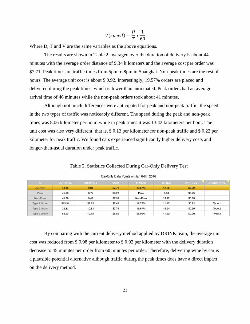
The results are shown in Table 2, averaged over the duration of delivery is about 44

minutes with the average order distance of 9.34 kilometers and the average cost per order was

$7.71. Peak times are traffic times from 5pm to 8pm in Shanghai. Non-peak times are the rest of

hours. The average unit cost is about $ 0.92. Interestingly, 19.57% orders are placed and

delivered during the peak times, which is fewer than anticipated. Peak orders had an average

arrival time of 46 minutes while the non-peak orders took about 41 minutes.

Although not much differences were anticipated for peak and non-peak traffic, the speed

in the two types of traffic was noticeably different. The speed during the peak and non-peak

times was 8.06 kilometer per hour, while in peak times it was 13.42 kilometers per hour. The

unit cost was also very different, that is, $ 0.13 per kilometer for non-peak traffic and $ 0.22 per

kilometer for peak traffic. We found cars experienced significantly higher delivery costs and

longer-than-usual duration under peak traffic.

By comparing with the current delivery method applied by DRINK team, the average unit

cost was reduced from $ 0.98 per kilometer to $ 0.92 per kilometer with the delivery duration

decrease to 45 minutes per order from 60 minutes per order. Therefore, delivering wine by car is

a plausible potential alternative although traffic during the peak times does have a direct impact

on the delivery method.

Table 2. Statistics Collected During Car-Only Delivery Test

24

5.1.3 Scenario II. Bike-Only Delivery

On January 10th, the management team from Drink-Më approved the mini-experiment

for the alternative method of delivery, that is, utilization of electronic bike only. The mini-test

would run for three days and be suspended at the discretion of the management subject to the

real operation data. The operation started at Shanghai Xuhui Administration area without any

promotions, which resulted in a usual pattern of order arrivals into the system.

For type I and II orders, system would process the order to either warehouse or third

party stores and the delivery team would pick up the order based on wherever the closest bike is.

For type III order, the system would let the bike pick up goods from either third party stores or

from the warehouse, whichever is closer to the rider, and then pick up the remaining items to

deliver. All orders would be delivered under a non-wait rule, which means the delivery team

would deliver even a single bottle for an inbound order. Unlike using cars, orders would not be

waited since the cost of delivering a bottle by bike is much lower than using a car.

Basically, the team collected the same type of data collected in Scenario I. However, a

slightly different formula was used for the cost of delivery. The cost in this experiment is

calculated by the formula that is used by financial department of Drink-Më:

C(Cost by Bike) =(T(Travel Duration) ∗

720 + D( Distances Travelled) ∗ 2/3 )

Currency Conversion Rate

Currency Conversion Rate: 1 USD = 6.51 CNY.

25

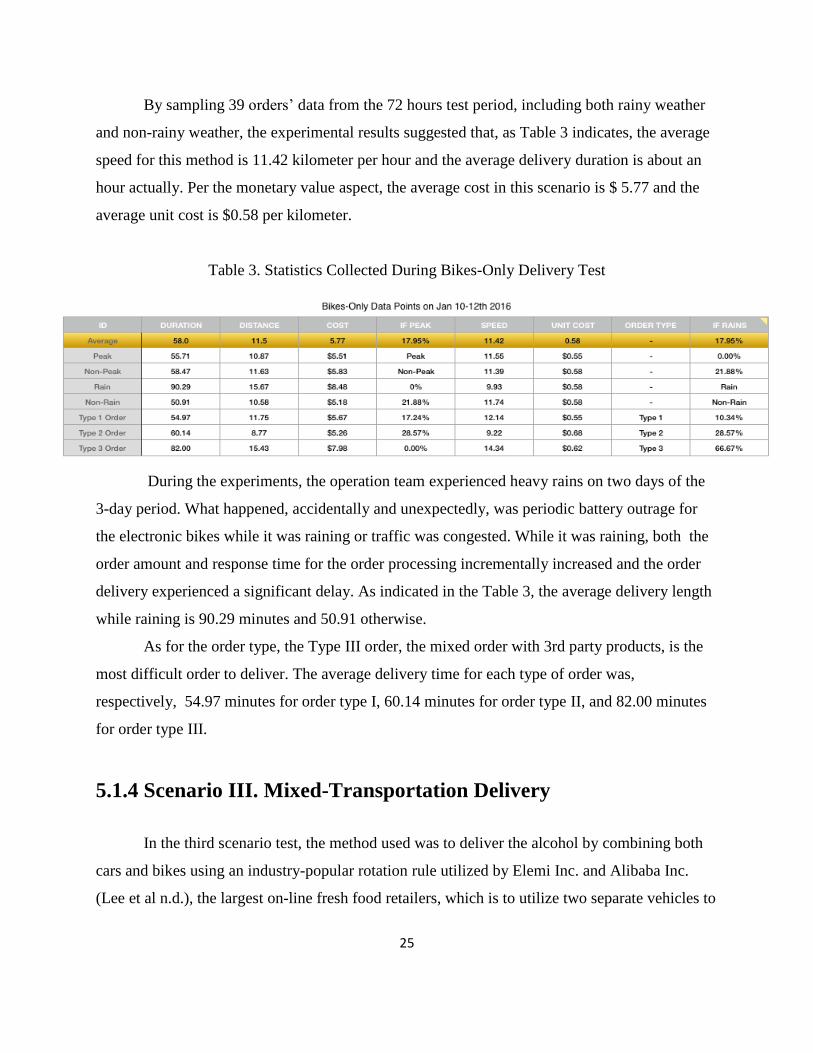
By sampling 39 orders’ data from the 72 hours test period, including both rainy weather

and non-rainy weather, the experimental results suggested that, as Table 3 indicates, the average

speed for this method is 11.42 kilometer per hour and the average delivery duration is about an

hour actually. Per the monetary value aspect, the average cost in this scenario is $ 5.77 and the

average unit cost is $0.58 per kilometer.

Table 3. Statistics Collected During Bikes-Only Delivery Test

During the experiments, the operation team experienced heavy rains on two days of the

3-day period. What happened, accidentally and unexpectedly, was periodic battery outrage for

the electronic bikes while it was raining or traffic was congested. While it was raining, both the

order amount and response time for the order processing incrementally increased and the order

delivery experienced a significant delay. As indicated in the Table 3, the average delivery length

while raining is 90.29 minutes and 50.91 otherwise.

As for the order type, the Type III order, the mixed order with 3rd party products, is the

most difficult order to deliver. The average delivery time for each type of order was,

respectively, 54.97 minutes for order type I, 60.14 minutes for order type II, and 82.00 minutes

for order type III.

5.1.4 Scenario III. Mixed-Transportation Delivery

In the third scenario test, the method used was to deliver the alcohol by combining both

cars and bikes using an industry-popular rotation rule utilized by Elemi Inc. and Alibaba Inc.

(Lee et al n.d.), the largest on-line fresh food retailers, which is to utilize two separate vehicles to

26

pick up goods and merge at some point, and then the order will finally be delivered by one of the

delivery employee. By considering two random locations of two vehicles and two different

delivery addresses, this methodology manages to reduce the transportation distance to a

relatively low level in order to minimize the cost.

However, in the real situation, the DRINK team owns two cars and several bikes at

warehouse location. Thus, in order to simulate this method, the team first freed all vehicles in

and around Shanghai. Since there is a condition that all vehicles would not be at warehouse

location or any other fixed point, thus, a wait rule was applied in this case, which is, if there is

only one order received, the order will not processed until the next order appeared. The

exception happened if the wait time is over 30 minutes. This rule is universally used in China for

companies do not obtain a permanent location for delivery vehicles or do not have self-owned

delivery vehicles.

For type I and II order, system would process the order to either warehouse or third party

stores. When orders are received, the wait rule indicates that the first order will wait until the

second one is received. The order to deliver first would be the one that is closer to the departure

point of vehicle. Then the one that is farther would be delivered second, regardless of the order

arrival time. The delivery team, processing this order, would use the car to pick up orders

and deliver the first order and then meet the bike rider at some point to have the bike-rider

to deliver the second order. However, if the wait time is more than 30 minutes after the first

order has been receiver, the first order would be delivered to the customer directly.

For type III orders, however, the system would undergo a non-wait rule. First, the

car would be sent to pick goods from warehouse products, and then the car would get in touch

with bike rider to merge at an optimal location that is calculated by embedded GPS system

supported by Map of Gaode, the top mobile map in China.

On December 19th, the management team from Drink-Më approved the mini-test for the

new method of delivery. At the beginning of the experiments, with only 6 orders, however, there

were long delays for every order that caused the experiments to suspend immediately. The

company received abnormal complaints from three customers regarding the irregular operations.

Subject to product reputation and customer satisfaction, the team had to stop the experiment,

which makes this solution infeasible for future operations. The results are shown in Table 4.

27

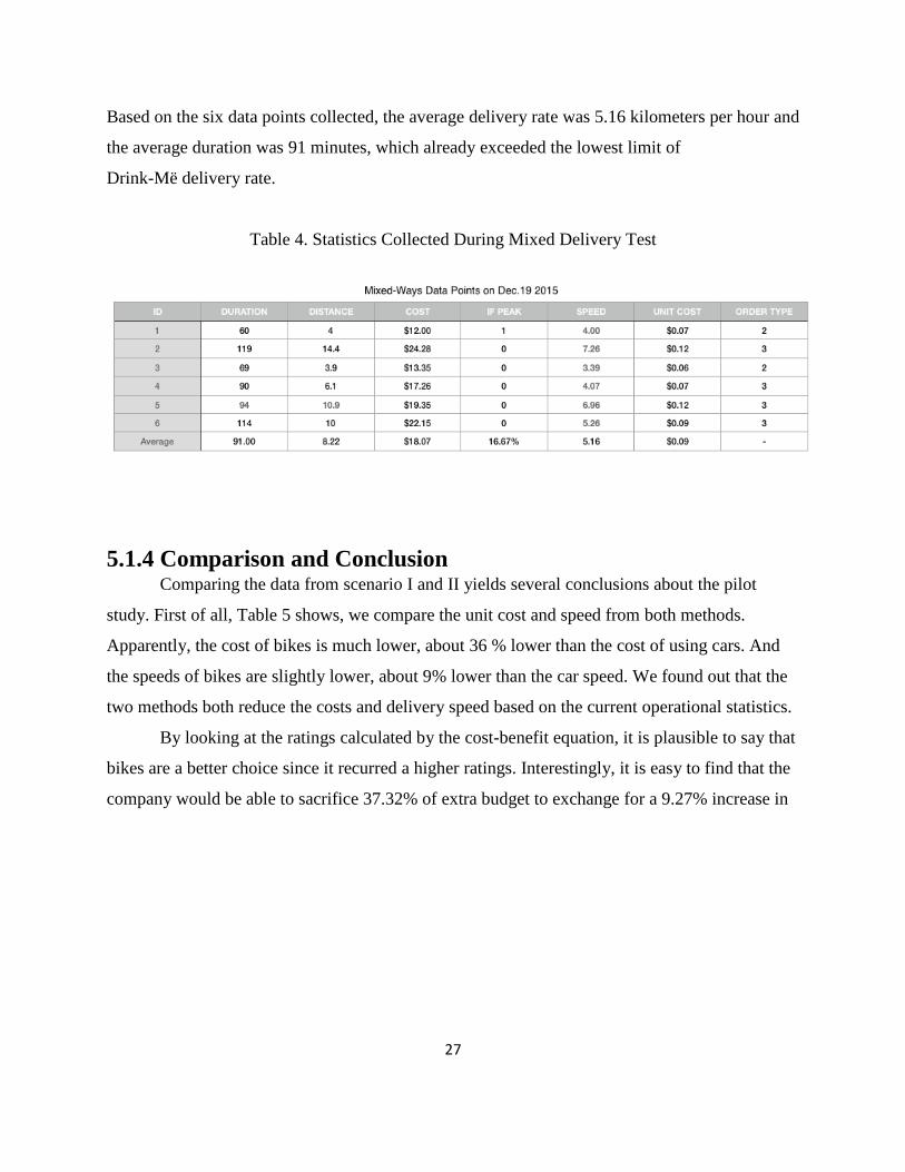
Based on the six data points collected, the average delivery rate was 5.16 kilometers per hour and

the average duration was 91 minutes, which already exceeded the lowest limit of

Drink-Më delivery rate.

Table 4. Statistics Collected During Mixed Delivery Test

5.1.4 Comparison and Conclusion Comparing the data from scenario I and II yields several conclusions about the pilot

study. First of all, Table 5 shows, we compare the unit cost and speed from both methods.

Apparently, the cost of bikes is much lower, about 36 % lower than the cost of using cars. And

the speeds of bikes are slightly lower, about 9% lower than the car speed. We found out that the

two methods both reduce the costs and delivery speed based on the current operational statistics.

By looking at the ratings calculated by the cost-benefit equation, it is plausible to say that

bikes are a better choice since it recurred a higher ratings. Interestingly, it is easy to find that the

company would be able to sacrifice 37.32% of extra budget to exchange for a 9.27% increase in

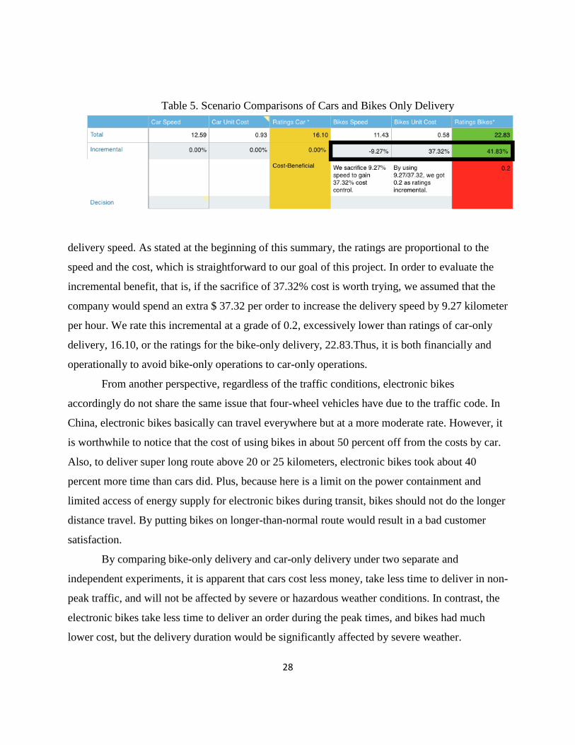
28

delivery speed. As stated at the beginning of this summary, the ratings are proportional to the

speed and the cost, which is straightforward to our goal of this project. In order to evaluate the

incremental benefit, that is, if the sacrifice of 37.32% cost is worth trying, we assumed that the

company would spend an extra $ 37.32 per order to increase the delivery speed by 9.27 kilometer

per hour. We rate this incremental at a grade of 0.2, excessively lower than ratings of car-only

delivery, 16.10, or the ratings for the bike-only delivery, 22.83.Thus, it is both financially and

operationally to avoid bike-only operations to car-only operations.

From another perspective, regardless of the traffic conditions, electronic bikes

accordingly do not share the same issue that four-wheel vehicles have due to the traffic code. In

China, electronic bikes basically can travel everywhere but at a more moderate rate. However, it

is worthwhile to notice that the cost of using bikes in about 50 percent off from the costs by car.

Also, to deliver super long route above 20 or 25 kilometers, electronic bikes took about 40

percent more time than cars did. Plus, because here is a limit on the power containment and

limited access of energy supply for electronic bikes during transit, bikes should not do the longer

distance travel. By putting bikes on longer-than-normal route would result in a bad customer

satisfaction.

By comparing bike-only delivery and car-only delivery under two separate and

independent experiments, it is apparent that cars cost less money, take less time to deliver in non-

peak traffic, and will not be affected by severe or hazardous weather conditions. In contrast, the

electronic bikes take less time to deliver an order during the peak times, and bikes had much

lower cost, but the delivery duration would be significantly affected by severe weather.

Table 5. Scenario Comparisons of Cars and Bikes Only Delivery

29

Conclusively speaking, based on the results from the two experiments, it is reasonable to

suggest that if the company would like to lower cost only, electronic bikes are the most

economical way. If the company would like to improve delivery speed, using cars as a

supplement, incuring a slightly higher cost, would be the most cost-effective way by not

triggering that 37 percent of increased budget.

5.2 Model Revision after Pilot Study

The findings we developed from Objective 3: Develop a Simulation Models came from

running different pilot experiments and comparing the results. This section describes the model

changes made after the real-time pilot study. We utilized data collected during the pilot study in

Section 5.1 and used it to develop input distributions for the modules in Arena to yield a more

accurate model. The analysis in the pilot study also generated a more accurate design to reflect

how orders flow in the system, when the system should stop accepting orders and what attributes

affect the delivery time in reality. In order to validate the model, the team utilized the Input

Analyzer to figure out the distribution type and parameters based on data from the pilot study.

5.2.1 Input Analyzer The Input Analyzer in Arena is used to fit probability distributions to data and to evaluate the

fit. Before using the Input Analyzer, we entered our data from an excel file from pilot study into

a text file ending with ******.DST. By doing this, the distribution type of the duration travelled,

distance travelled and other important from the pilot study were obtained. The distributions and

graphs that were used in the model are described below.

30

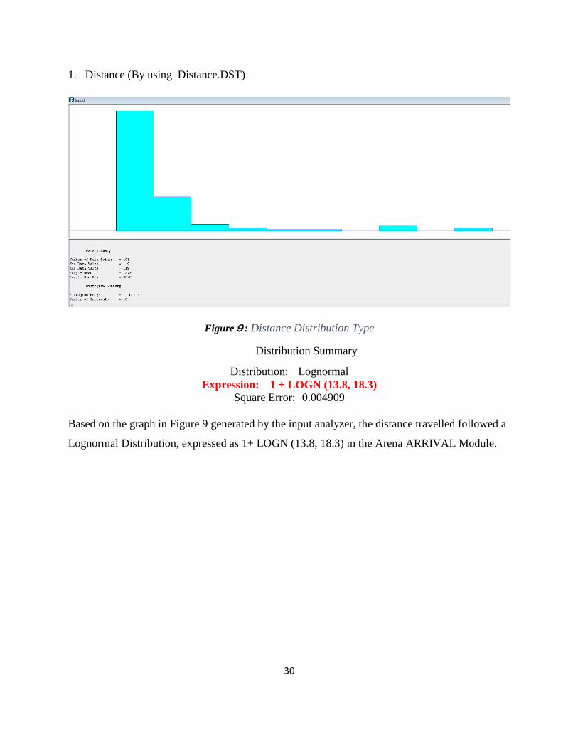
1. Distance (By using Distance.DST)

Figure９: Distance Distribution Type

Distribution Summary

Distribution: Lognormal

Expression: 1 + LOGN (13.8, 18.3)

Square Error: 0.004909

Based on the graph in Figure 9 generated by the input analyzer, the distance travelled followed a

Lognormal Distribution, expressed as 1+ LOGN (13.8, 18.3) in the Arena ARRIVAL Module.

31

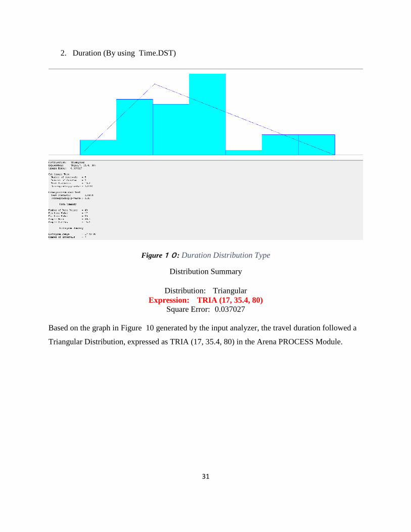
2. Duration (By using Time.DST)

Figure１０: Duration Distribution Type


Distribution: Triangular

Expression: TRIA (17, 35.4, 80)


Based on the graph in Figure 10 generated by the input analyzer, the travel duration followed a

Triangular Distribution, expressed as TRIA (17, 35.4, 80) in the Arena PROCESS Module.

32

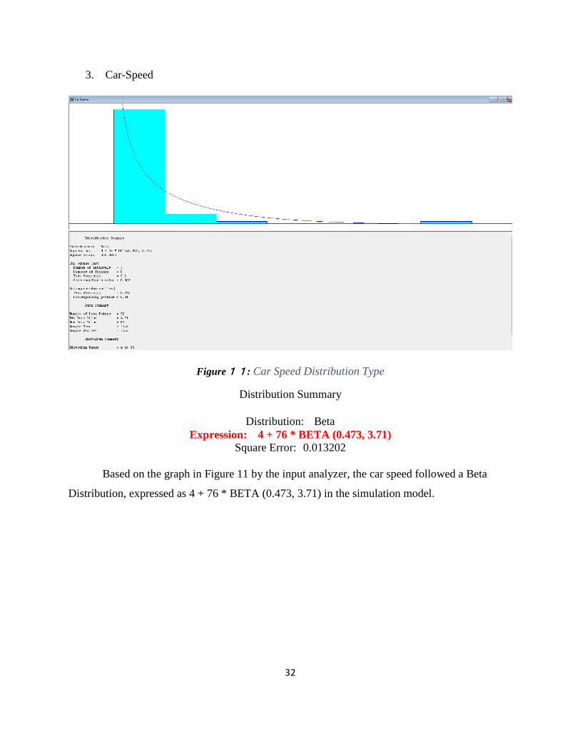
3. Car-Speed

Figure１１: Car Speed Distribution Type


Distribution: Beta

Expression: 4 + 76 * BETA (0.473, 3.71)


Based on the graph in Figure 11 by the input analyzer, the car speed followed a Beta

Distribution, expressed as 4 + 76 * BETA (0.473, 3.71) in the simulation model.

33

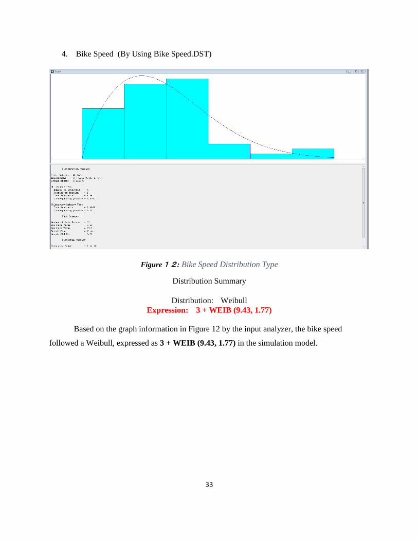
4. Bike Speed (By Using Bike Speed.DST)

Figure１２: Bike Speed Distribution Type


Distribution: Weibull

Expression: 3 + WEIB (9.43, 1.77)

Based on the graph information in Figure 12 by the input analyzer, the bike speed

followed a Weibull, expressed as 3 + WEIB (9.43, 1.77) in the simulation model.

34

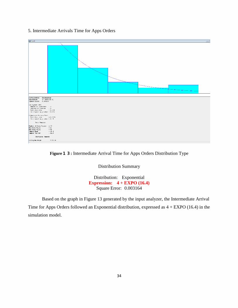
5. Intermediate Arrivals Time for Apps Orders

Figure１３: Intermediate Arrival Time for Apps Orders Distribution Type


Distribution: Exponential

Expression: 4 + EXPO (16.4)


Based on the graph in Figure 13 generated by the input analyzer, the Intermediate Arrival

Time for Apps Orders followed an Exponential distribution, expressed as 4 + EXPO (16.4) in the

simulation model.

35

6. Intermediate Arrival Time for Web Orders

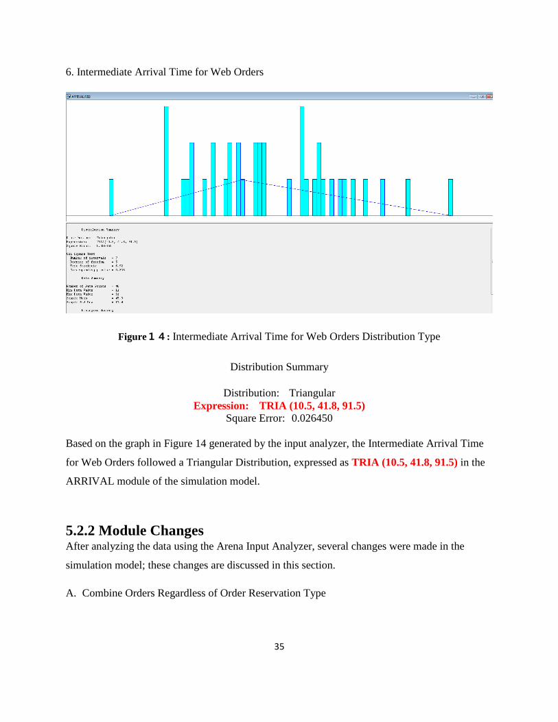
Figure１４: Intermediate Arrival Time for Web Orders Distribution Type


Distribution: Triangular

Expression: TRIA (10.5, 41.8, 91.5)


Based on the graph in Figure 14 generated by the input analyzer, the Intermediate Arrival Time

for Web Orders followed a Triangular Distribution, expressed as TRIA (10.5, 41.8, 91.5) in the

ARRIVAL module of the simulation model.

5.2.2 Module Changes After analyzing the data using the Arena Input Analyzer, several changes were made in the

simulation model; these changes are discussed in this section.

A. Combine Orders Regardless of Order Reservation Type

36

In the original model, orders were divided into two types: reservations or instant orders,

because we believed that order processing might be different for each type. However, in the real

operations, orders with reservation will be automatically processed as instant orders while falling

into a specific time window, which is 75 minutes. By eliminating the [Reserved Order] module

in the arrivals section, the whole system not only becomes simpler but also concentrates more on

improving the overall efficiency.

B. Delete Delivery Station in Arrival Section

The delivery station was used to simulate the order processing time, which in the revised

model is simulated by [App Order Process], since the delivery station is the station that handles

the order.

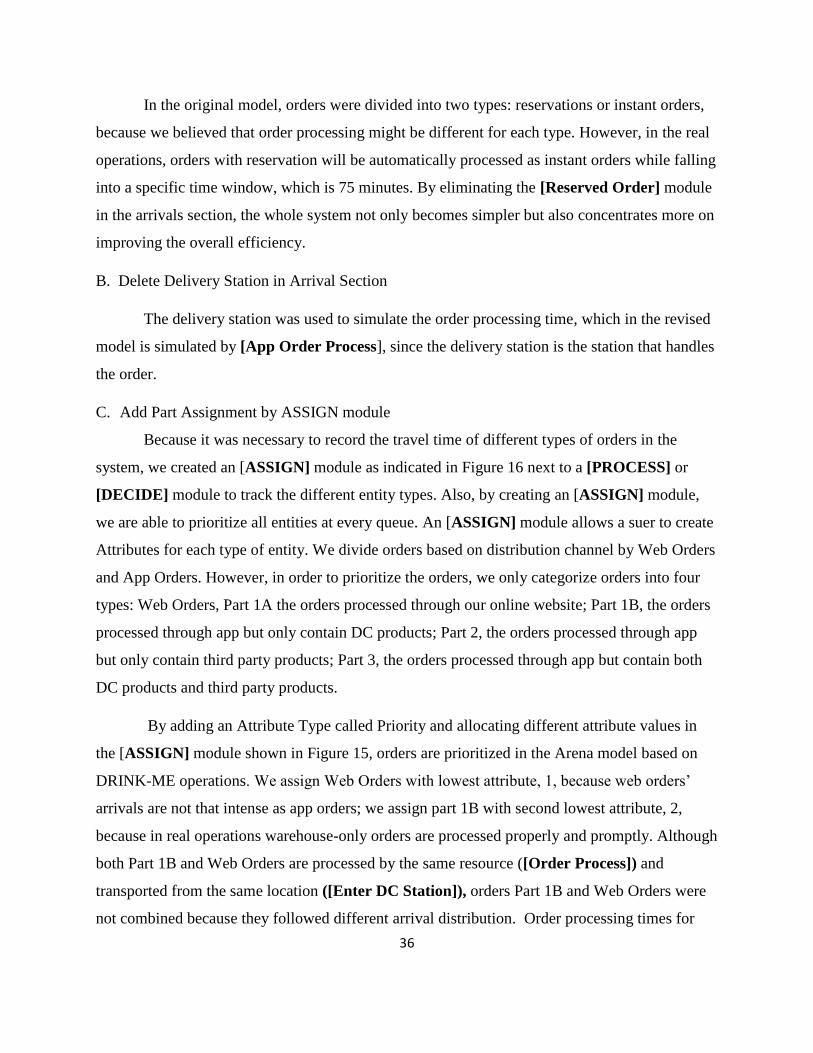
C. Add Part Assignment by ASSIGN module

Because it was necessary to record the travel time of different types of orders in the

system, we created an [ASSIGN] module as indicated in Figure 16 next to a [PROCESS] or

[DECIDE] module to track the different entity types. Also, by creating an [ASSIGN] module,

we are able to prioritize all entities at every queue. An [ASSIGN] module allows a suer to create

Attributes for each type of entity. We divide orders based on distribution channel by Web Orders

and App Orders. However, in order to prioritize the orders, we only categorize orders into four

types: Web Orders, Part 1A the orders processed through our online website; Part 1B, the orders

processed through app but only contain DC products; Part 2, the orders processed through app

but only contain third party products; Part 3, the orders processed through app but contain both

DC products and third party products.

By adding an Attribute Type called Priority and allocating different attribute values in

the [ASSIGN] module shown in Figure 15, orders are prioritized in the Arena model based on

DRINK-ME operations. We assign Web Orders with lowest attribute, 1, because web orders’

arrivals are not that intense as app orders; we assign part 1B with second lowest attribute, 2,

because in real operations warehouse-only orders are processed properly and promptly. Although

both Part 1B and Web Orders are processed by the same resource ([Order Process]) and

transported from the same location ([Enter DC Station]), orders Part 1B and Web Orders were

not combined because they followed different arrival distribution. Order processing times for

37

Web Orders are also normally longer than Apps Orders. The attribute value, 3, was applied to

Part 2 orders that contain only third party goods, because the third party only orders always

require a little bit more delivery time than Part 1B orders. Finally, the highest priority value,3, is

assigned with the hardest delivery option, Part 3, the orders that require a pickup procedure at

both warehouse and third party stores before delivery. In order to facilitate the observation of the

movement of entities, we assigned Entity.Picutre to each type of order based on their priority

values; a green ball, blue ball, yellow ball and red ball were assigned to Web Orders, Part 1B,

Part 2, Part 3, respectively.

Figure １５: ASSIGN Module Parameter Window

D. Resources Complexity and Set Rule

In DRINK-ME’s real operation, there are 8 vehicles with either 8 bike-riders or 8 car-

drivers most of time. Thus, we created 8 persons in our resources named: Ada, Bob, Charlie,

David, Edward, Hermine, Frank, George, who would work as either drivers or riders in our

Arena system. Since we observed that all employees were distributed in a cyclic order in the

operation, we designed a [Set] order that contains eight identical employees. In the

[RESOURCE] module, all employees have fixed capacity, which did not reflect the real

operational situation. However, when resources were modeled separately and according to a

schedule, the model was not seizing the resources correctly. The fixed-capacity assumption did

38

not influence the simulation results actually. Hence, in this case, it is understandable to

compromise on the resource capacity issue by choosing fixed capacity.

E. Changes to Process Modules

In all delivery [PROCESS] modules, based on a Set rule, we chose the [SET] Tab

instead of [Resource] in the Resource Tab in Arena software. The set will follow a cyclic rule

for selecting which employee to deliver a particular order.

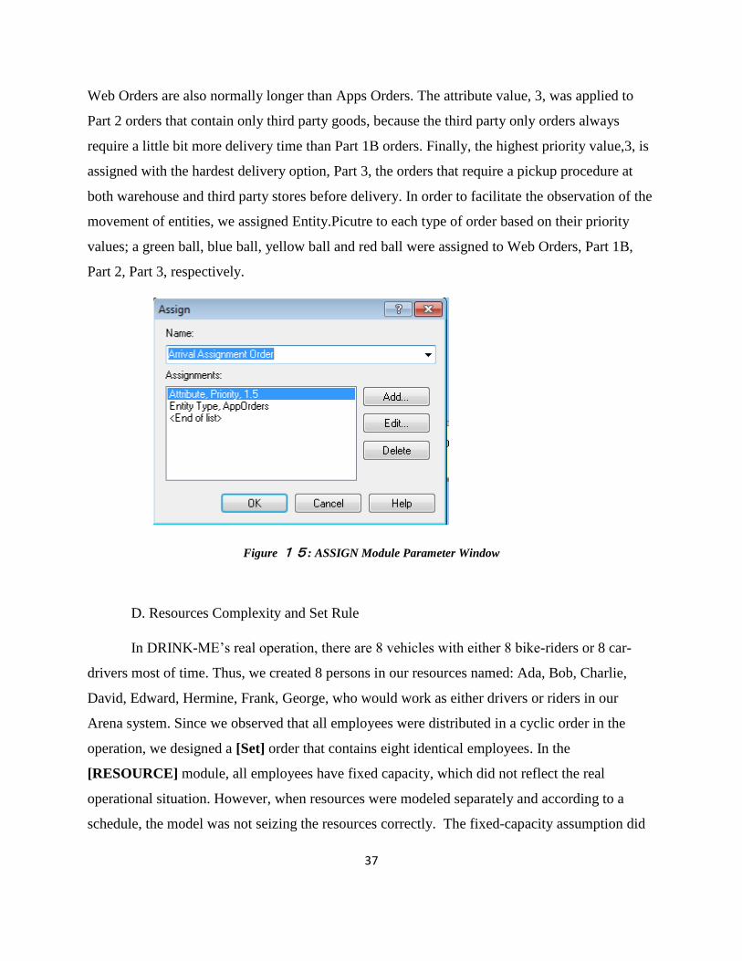
F. Add Arrival Cut-Off Logic

In our pilot study, we found out that DRINKME operated from 8a.m. to 1 a.m., while the

last order time is 12 a.m. and all orders in the system would be delivered by 1 a.m. As indicated

in Figure 16, the team created an arrival cutoff to comply with pilot study. We “faked” an arrival

after “TNOW>=960” , which means 16 hours after operation starts, the simulation system would

automatically lead all arrival entities into this cutoff station used to “choke off” the arrival stream

at 12am. We did this by creating a single “logical” entity at time 960 min. (12am) to delete all

arrivals and set up Time Between Arrivals at 999999 min., and Max Arrivals at 1 as indicated in

Figure 17. Next, we used an [Assign] module to set the variable MaxOrders to 1 for Max

Arrivals in the Create module for attempted orders and then dispose of this single logical entity

using a Cutoff module.

Figure １６: Arrival Cut-Off Logic

39

Figure１７: CREATE module at Arrival Cut-off Section

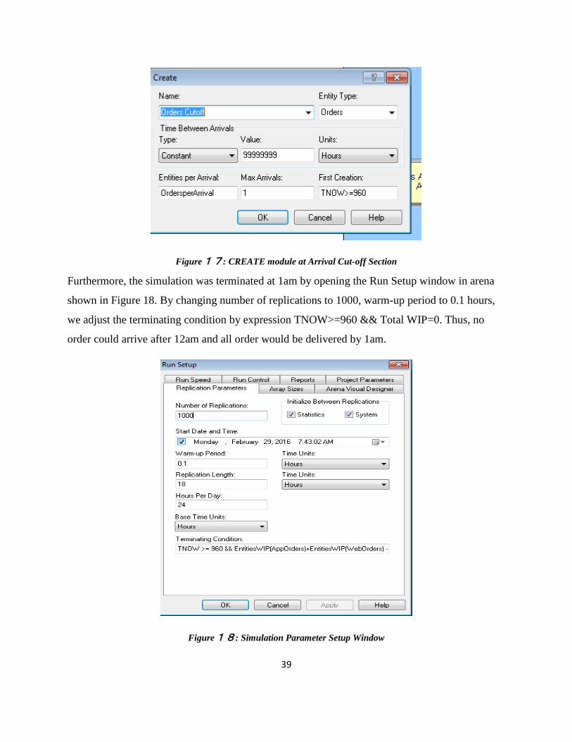
Furthermore, the simulation was terminated at 1am by opening the Run Setup window in arena

shown in Figure 18. By changing number of replications to 1000, warm-up period to 0.1 hours,

we adjust the terminating condition by expression TNOW>=960 && Total WIP=0. Thus, no

order could arrive after 12am and all order would be delivered by 1am.

Figure１８: Simulation Parameter Setup Window

40

5.2.3 Adding Data to the Model

Data from the pilot study was incorporated into the model as described below:

(1) From Part II, we determined inter-arrival times for each type of order.

(2) For WEB orders, the arrivals follow a triangular distribution with TRIA (10.5, 41.8, 91.5)

minutes.

(3) For App orders, the arrivals follow an exponential distribution with 4+EXPO (16.4).

(4) Based on data from pilot study, we found out that 12.94% of data are from a 3rd

party. So, we

used this percentage at the 2-way by chance DECIDE Module to determine order type,

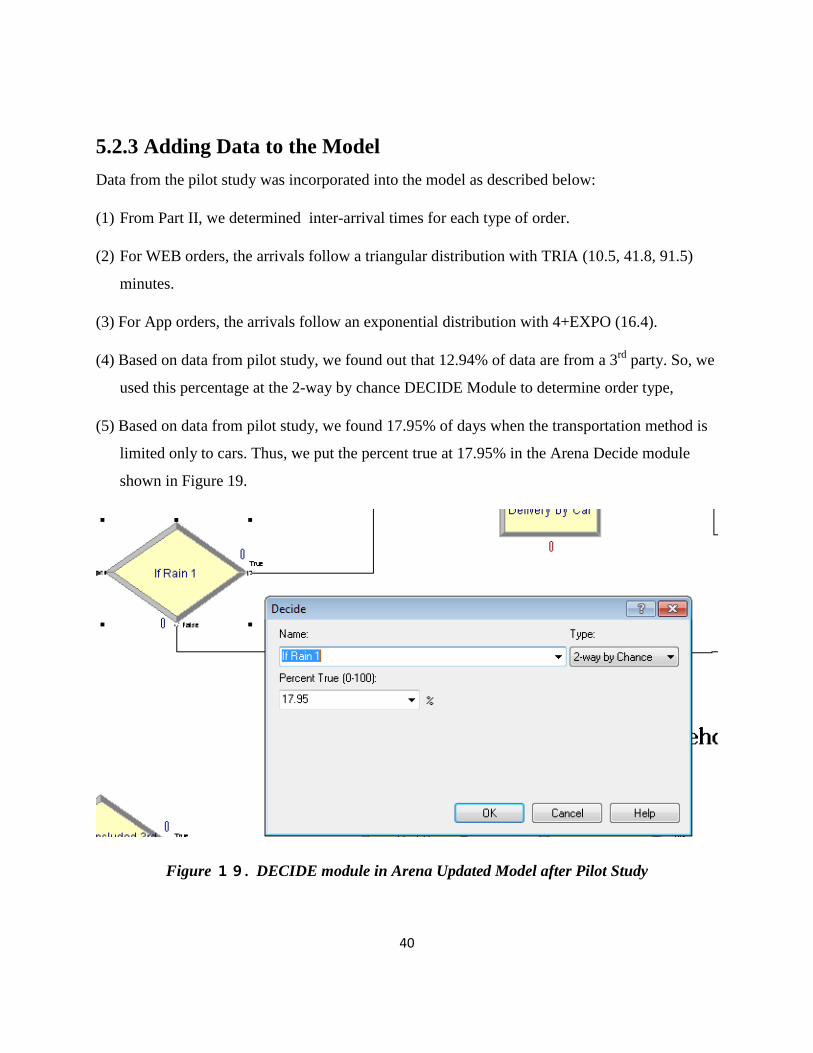
(5) Based on data from pilot study, we found 17.95% of days when the transportation method is

limited only to cars. Thus, we put the percent true at 17.95% in the Arena Decide module

shown in Figure 19.

Figure １９. DECIDE module in Arena Updated Model after Pilot Study

41

5.3 Simulation Results

After simulating, we found the current best scenario was 6 bikes, 2 cars and 3

administrative order takers. The overall order processing time was 1.167 hours for Type III

order, 0.9 hours for Type II order and 1.046 hours for Type IB order, which reduces the current

travel time at DRINK-ME by 12.50%. In practice, the travel time are averaged over 1.33 hours

for Type III orders. However, the car utilization is 0.283; the bike utilization is 0.576; the order

processing admin utilization is 0.064. Because each resource represents two staff and staff are

cost-related, the utilization of the car and bike is too low. Thus, it is not a feasible and cost-

effective solution for a company to run at such low efficiency. Thus, our scenario analysis

focused primarily on improving the efficiency.

5.4 Scenario Analysis

The findings we developed as part of Objective 4: Simulation Experiments came from the

simulation results of more than 10,000 trials among 10 scenarios. The original scenario came

from our best findings in the Pilot Study. This best option was evaluated and compared with the

10 scenarios developed and the results are discussed here. Also, knowing that the original

scenario was the best scenario from Pilot Study, we expected to find better results in simulation.

First, we ran the original scenario for 100 replications in the Process Analyzer by creating

a PAN file in the same folder as the simulation model. By inserting all resources as controls and

the travel time of three order types and utilization rate of three resources as responses, a scenario

comparison portal was created. The results of the different scenarios tested are described below.

A. Original Scenario 6 Bikes 2 Cars 3 Order Processing Admins

As indicated in Figure 20, car utilization is low in the original scenario. So we tried

improving the utilization rate by reducing the number of cars to 1 and increasing the number of

bikes to 7 while maintaining the same number of admins. This change is captured as Scenario 1.

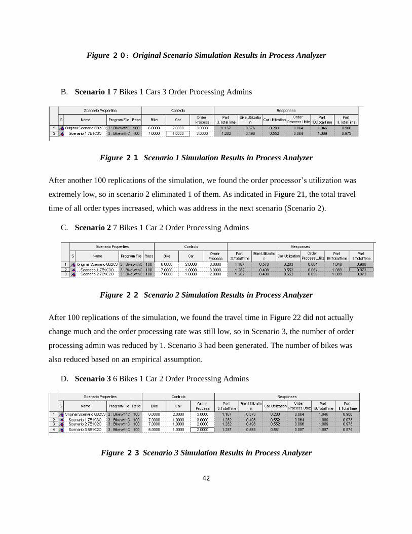
42

Figure ２０: Original Scenario Simulation Results in Process Analyzer

B. Scenario 1 7 Bikes 1 Cars 3 Order Processing Admins

Figure ２１ Scenario 1 Simulation Results in Process Analyzer

After another 100 replications of the simulation, we found the order processor’s utilization was

extremely low, so in scenario 2 eliminated 1 of them. As indicated in Figure 21, the total travel

time of all order types increased, which was address in the next scenario (Scenario 2).

C. Scenario 2 7 Bikes 1 Car 2 Order Processing Admins

Figure ２２ Scenario 2 Simulation Results in Process Analyzer

After 100 replications of the simulation, we found the travel time in Figure 22 did not actually

change much and the order processing rate was still low, so in Scenario 3, the number of order

processing admin was reduced by 1. Scenario 3 had been generated. The number of bikes was

also reduced based on an empirical assumption.

D. Scenario 3 6 Bikes 1 Car 2 Order Processing Admins

Figure ２３ Scenario 3 Simulation Results in Process Analyzer

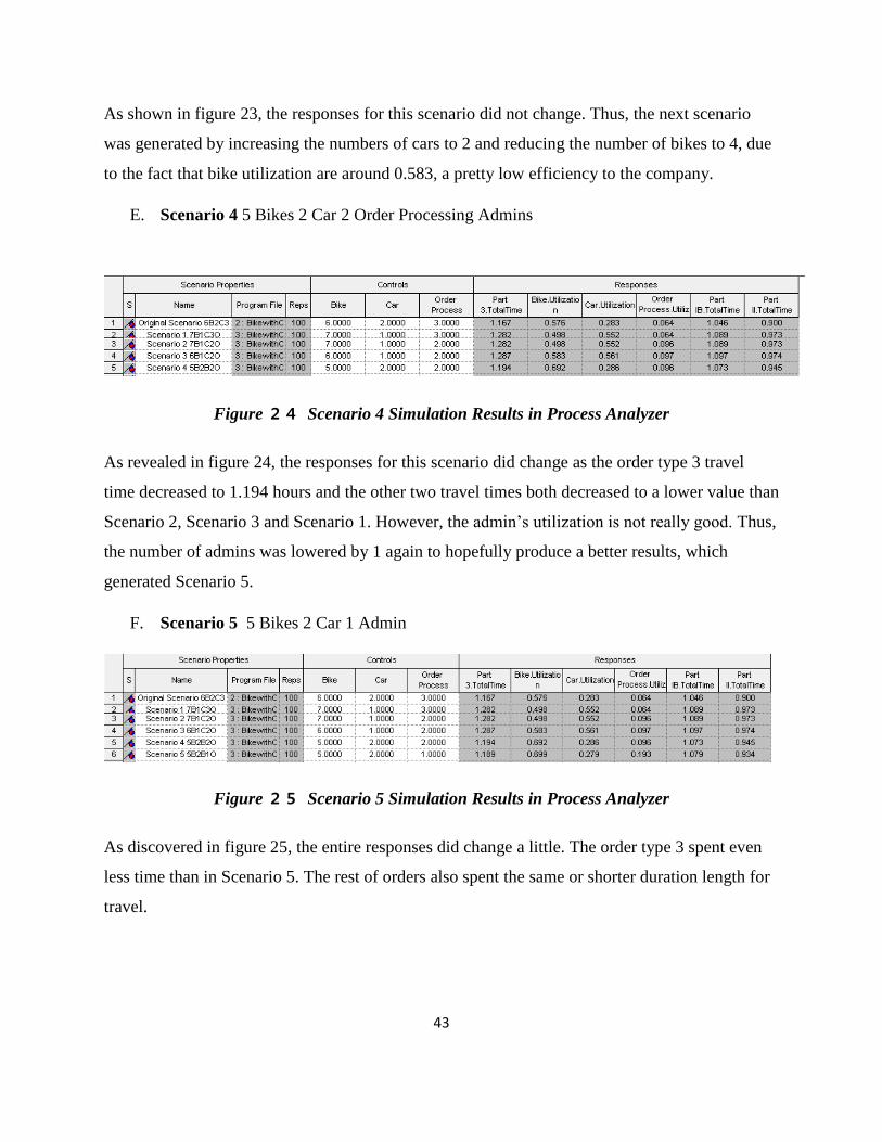
43

As shown in figure 23, the responses for this scenario did not change. Thus, the next scenario

was generated by increasing the numbers of cars to 2 and reducing the number of bikes to 4, due

to the fact that bike utilization are around 0.583, a pretty low efficiency to the company.

E. Scenario 4 5 Bikes 2 Car 2 Order Processing Admins

Figure ２４ Scenario 4 Simulation Results in Process Analyzer

As revealed in figure 24, the responses for this scenario did change as the order type 3 travel

time decreased to 1.194 hours and the other two travel times both decreased to a lower value than

Scenario 2, Scenario 3 and Scenario 1. However, the admin’s utilization is not really good. Thus,

the number of admins was lowered by 1 again to hopefully produce a better results, which

generated Scenario 5.

F. Scenario 5 5 Bikes 2 Car 1 Admin

Figure ２５ Scenario 5 Simulation Results in Process Analyzer

As discovered in figure 25, the entire responses did change a little. The order type 3 spent even

less time than in Scenario 5. The rest of orders also spent the same or shorter duration length for

travel.

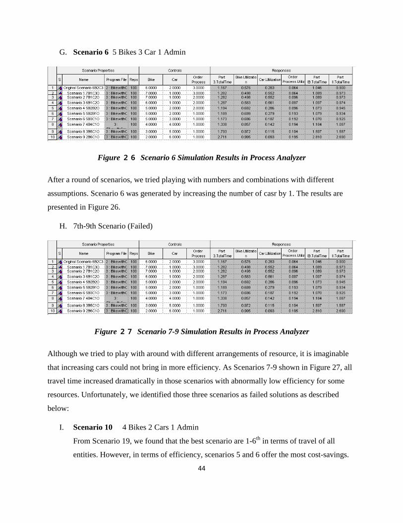
44

G. Scenario 6 5 Bikes 3 Car 1 Admin

Figure ２６ Scenario 6 Simulation Results in Process Analyzer

After a round of scenarios, we tried playing with numbers and combinations with different

assumptions. Scenario 6 was generated by increasing the number of casr by 1. The results are

presented in Figure 26.

H. 7th-9th Scenario (Failed)

Figure ２７ Scenario 7-9 Simulation Results in Process Analyzer

Although we tried to play with around with different arrangements of resource, it is imaginable

that increasing cars could not bring in more efficiency. As Scenarios 7-9 shown in Figure 27, all

travel time increased dramatically in those scenarios with abnormally low efficiency for some

resources. Unfortunately, we identified those three scenarios as failed solutions as described

below:

I. Scenario 10 4 Bikes 2 Cars 1 Admin

From Scenario 19, we found that the best scenario are 1-6th

in terms of travel of all

entities. However, in terms of efficiency, scenarios 5 and 6 offer the most cost-savings.

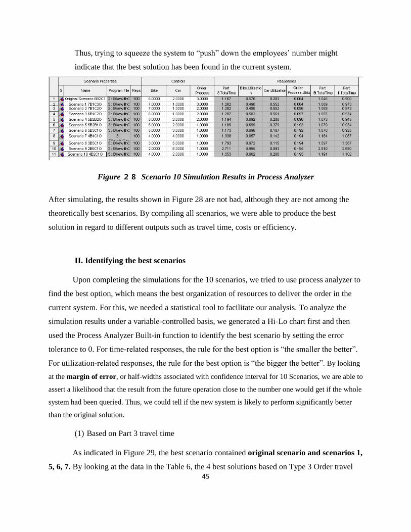
45

Thus, trying to squeeze the system to “push” down the employees’ number might

indicate that the best solution has been found in the current system.

Figure ２８ Scenario 10 Simulation Results in Process Analyzer

After simulating, the results shown in Figure 28 are not bad, although they are not among the

theoretically best scenarios. By compiling all scenarios, we were able to produce the best

solution in regard to different outputs such as travel time, costs or efficiency.

II. Identifying the best scenarios

Upon completing the simulations for the 10 scenarios, we tried to use process analyzer to

find the best option, which means the best organization of resources to deliver the order in the

current system. For this, we needed a statistical tool to facilitate our analysis. To analyze the

simulation results under a variable-controlled basis, we generated a Hi-Lo chart first and then

used the Process Analyzer Built-in function to identify the best scenario by setting the error

tolerance to 0. For time-related responses, the rule for the best option is “the smaller the better”.

For utilization-related responses, the rule for the best option is “the bigger the better”. By looking

at the margin of error, or half-widths associated with confidence interval for 10 Scenarios, we are able to

assert a likelihood that the result from the future operation close to the number one would get if the whole

system had been queried. Thus, we could tell if the new system is likely to perform significantly better

than the original solution.

(1) Based on Part 3 travel time

As indicated in Figure 29, the best scenario contained original scenario and scenarios 1,

5, 6, 7. By looking at the data in the Table 6, the 4 best solutions based on Type 3 Order travel

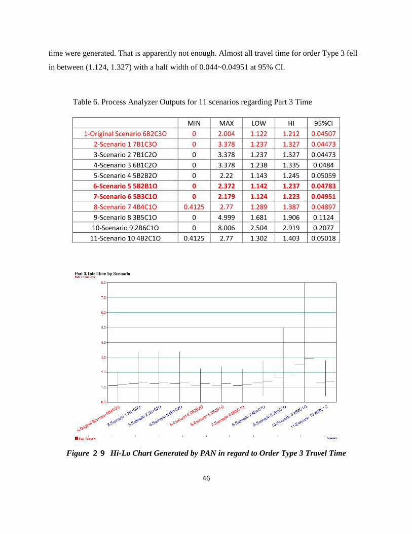
46

time were generated. That is apparently not enough. Almost all travel time for order Type 3 fell

in between (1.124, 1.327) with a half width of 0.044~0.04951 at 95% CI.

Table 6. Process Analyzer Outputs for 11 scenarios regarding Part 3 Time

Figure ２９ Hi-Lo Chart Generated by PAN in regard to Order Type 3 Travel Time

MIN MAX LOW HI 95%CI

1-Original Scenario 6B2C3O 0 2.004 1.122 1.212 0.04507

2-Scenario 1 7B1C3O 0 3.378 1.237 1.327 0.04473

3-Scenario 2 7B1C2O 0 3.378 1.237 1.327 0.04473

4-Scenario 3 6B1C2O 0 3.378 1.238 1.335 0.0484

5-Scenario 4 5B2B2O 0 2.22 1.143 1.245 0.05059

6-Scenario 5 5B2B1O 0 2.372 1.142 1.237 0.04783

7-Scenario 6 5B3C1O 0 2.179 1.124 1.223 0.04951

8-Scenario 7 4B4C1O 0.4125 2.77 1.289 1.387 0.04897

9-Scenario 8 3B5C1O 0 4.999 1.681 1.906 0.1124

10-Scenario 9 2B6C1O 0 8.006 2.504 2.919 0.2077

11-Scenario 10 4B2C1O 0.4125 2.77 1.302 1.403 0.05018

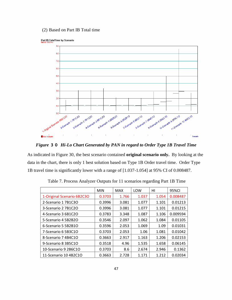
47

(2) Based on Part IB Total time

Figure ３０ Hi-Lo Chart Generated by PAN in regard to Order Type 1B Travel Time

As indicated in Figure 30, the best scenario contained original scenario only. By looking at the

data in the chart, there is only 1 best solution based on Type 1B Order travel time. Order Type

1B travel time is significantly lower with a range of [1.037-1.054] at 95% CI of 0.008487.

Table 7. Process Analyzer Outputs for 11 scenarios regarding Part 1B Time


1-Original Scenario 6B2C3O 0.3703 1.766 1.037 1.054 0.008487

2-Scenario 1 7B1C3O 0.3996 3.081 1.077 1.101 0.01213

3-Scenario 2 7B1C2O 0.3996 3.081 1.077 1.101 0.01215

4-Scenario 3 6B1C2O 0.3783 3.348 1.087 1.106 0.009594

5-Scenario 4 5B2B2O 0.3546 2.097 1.062 1.084 0.01105

6-Scenario 5 5B2B1O 0.3596 2.053 1.069 1.09 0.01031

7-Scenario 6 5B3C1O 0.3703 2.053 1.06 1.081 0.01042

8-Scenario 7 4B4C1O 0.3663 2.917 1.163 1.206 0.02153

9-Scenario 8 3B5C1O 0.3518 4.96 1.535 1.658 0.06145

10-Scenario 9 2B6C1O 0.3703 8.6 2.674 2.946 0.1362

11-Scenario 10 4B2C1O 0.3663 2.728 1.171 1.212 0.02034

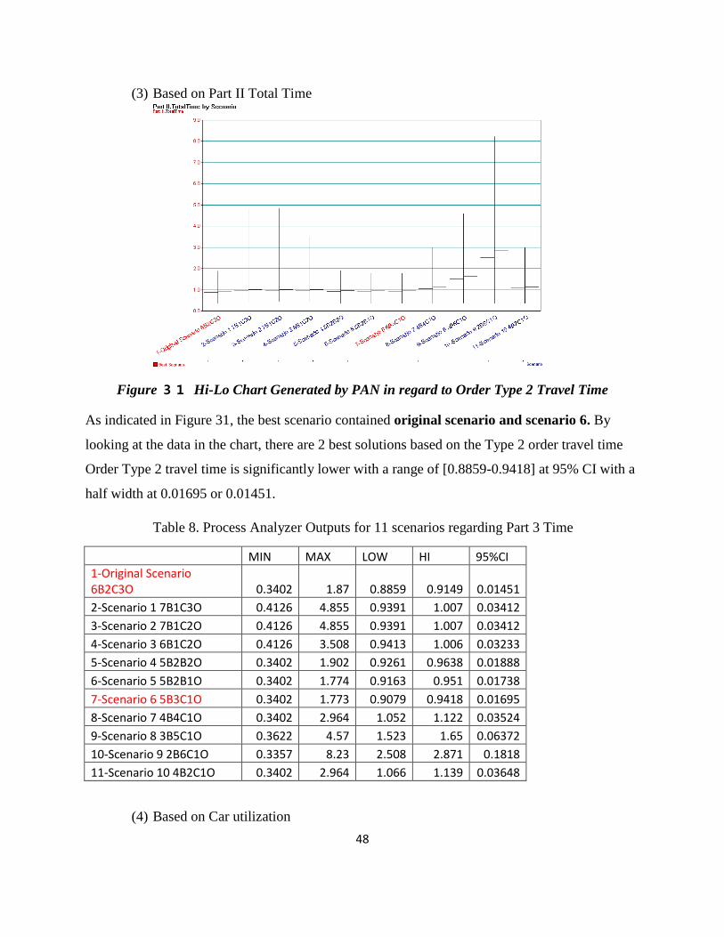
48

(3) Based on Part II Total Time

Figure ３１ Hi-Lo Chart Generated by PAN in regard to Order Type 2 Travel Time

As indicated in Figure 31, the best scenario contained original scenario and scenario 6. By

looking at the data in the chart, there are 2 best solutions based on the Type 2 order travel time

Order Type 2 travel time is significantly lower with a range of [0.8859-0.9418] at 95% CI with a

half width at 0.01695 or 0.01451.

Table 8. Process Analyzer Outputs for 11 scenarios regarding Part 3 Time


1-Original Scenario 6B2C3O 0.3402 1.87 0.8859 0.9149 0.01451

2-Scenario 1 7B1C3O 0.4126 4.855 0.9391 1.007 0.03412

3-Scenario 2 7B1C2O 0.4126 4.855 0.9391 1.007 0.03412

4-Scenario 3 6B1C2O 0.4126 3.508 0.9413 1.006 0.03233

5-Scenario 4 5B2B2O 0.3402 1.902 0.9261 0.9638 0.01888

6-Scenario 5 5B2B1O 0.3402 1.774 0.9163 0.951 0.01738

7-Scenario 6 5B3C1O 0.3402 1.773 0.9079 0.9418 0.01695

8-Scenario 7 4B4C1O 0.3402 2.964 1.052 1.122 0.03524

9-Scenario 8 3B5C1O 0.3622 4.57 1.523 1.65 0.06372

10-Scenario 9 2B6C1O 0.3357 8.23 2.508 2.871 0.1818

11-Scenario 10 4B2C1O 0.3402 2.964 1.066 1.139 0.03648

(4) Based on Car utilization

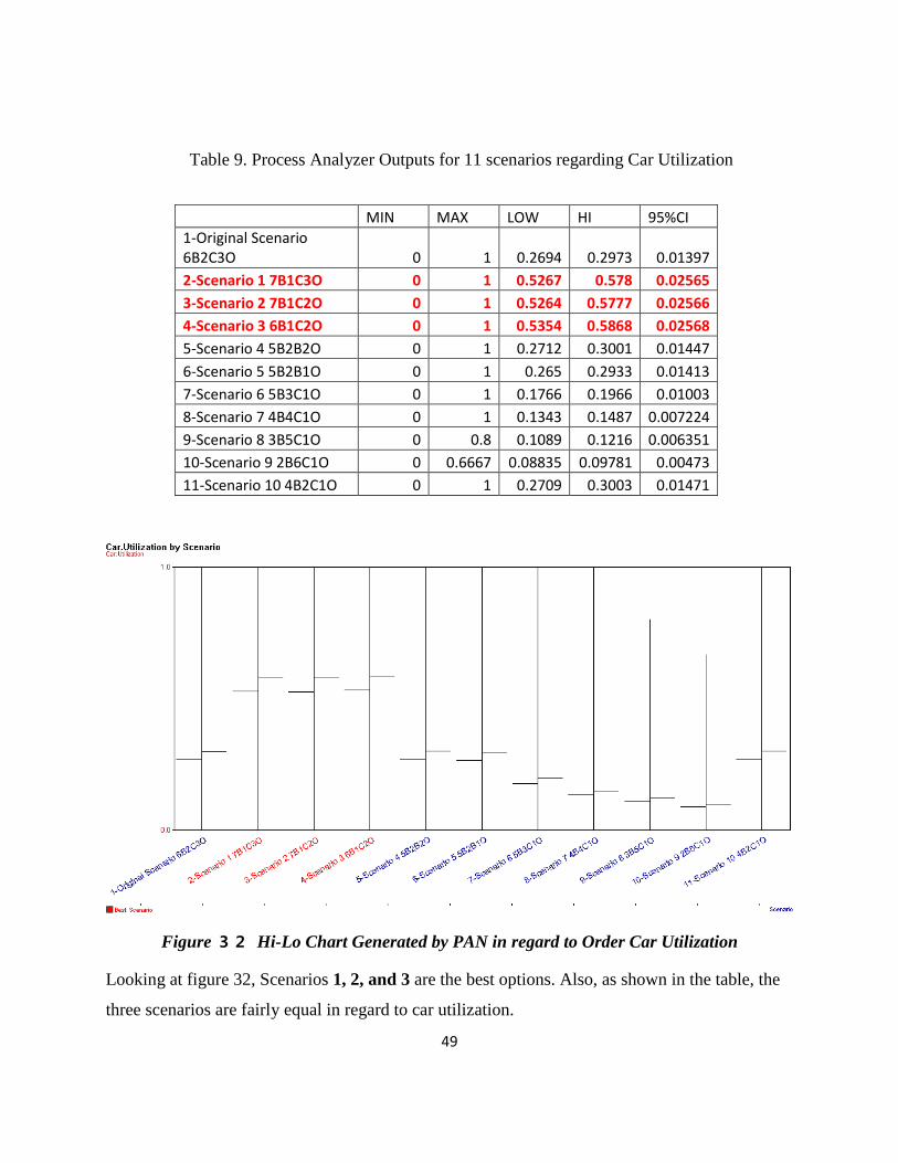
49

Table 9. Process Analyzer Outputs for 11 scenarios regarding Car Utilization

Figure ３２ Hi-Lo Chart Generated by PAN in regard to Order Car Utilization

Looking at figure 32, Scenarios 1, 2, and 3 are the best options. Also, as shown in the table, the

three scenarios are fairly equal in regard to car utilization.


1-Original Scenario 6B2C3O 0 1 0.2694 0.2973 0.01397

2-Scenario 1 7B1C3O 0 1 0.5267 0.578 0.02565

3-Scenario 2 7B1C2O 0 1 0.5264 0.5777 0.02566

4-Scenario 3 6B1C2O 0 1 0.5354 0.5868 0.02568

5-Scenario 4 5B2B2O 0 1 0.2712 0.3001 0.01447

6-Scenario 5 5B2B1O 0 1 0.265 0.2933 0.01413

7-Scenario 6 5B3C1O 0 1 0.1766 0.1966 0.01003

8-Scenario 7 4B4C1O 0 1 0.1343 0.1487 0.007224

9-Scenario 8 3B5C1O 0 0.8 0.1089 0.1216 0.006351

10-Scenario 9 2B6C1O 0 0.6667 0.08835 0.09781 0.00473

11-Scenario 10 4B2C1O 0 1 0.2709 0.3003 0.01471

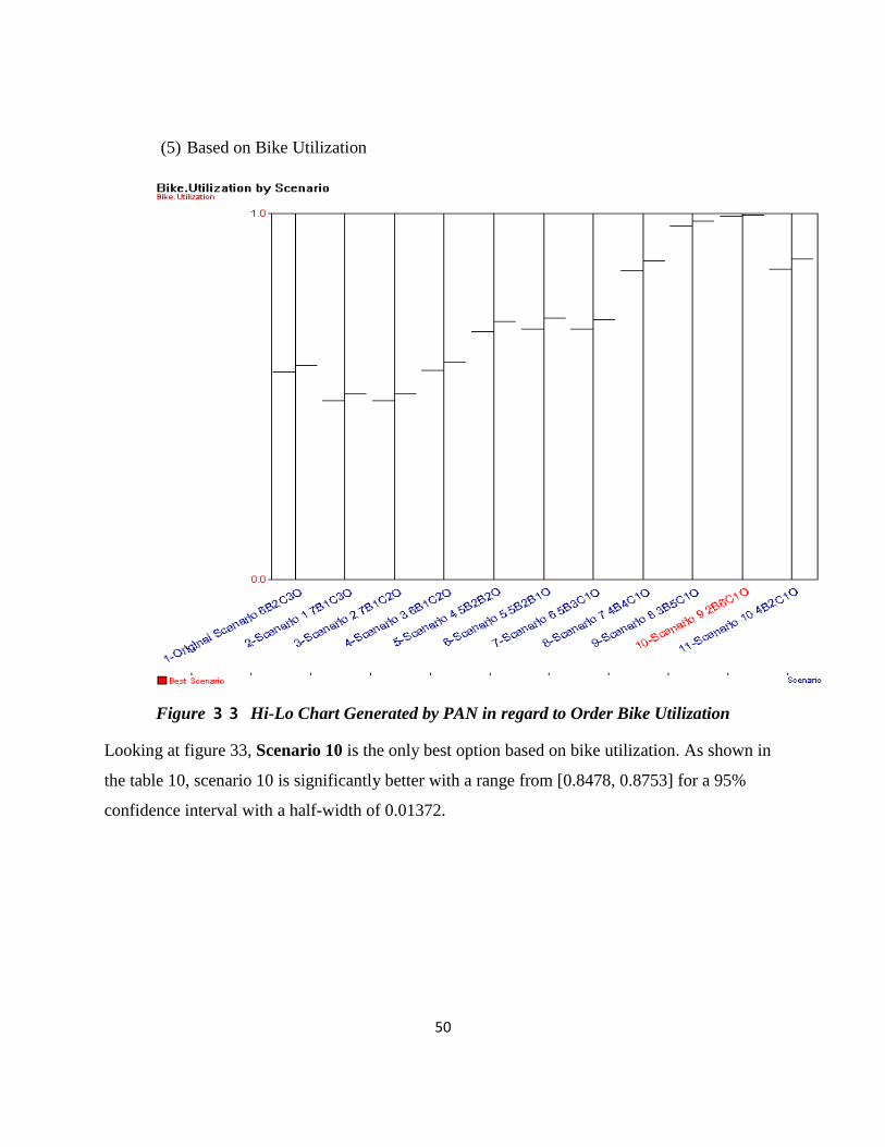
50

(5) Based on Bike Utilization

Figure ３３ Hi-Lo Chart Generated by PAN in regard to Order Bike Utilization

Looking at figure 33, Scenario 10 is the only best option based on bike utilization. As shown in

the table 10, scenario 10 is significantly better with a range from [0.8478, 0.8753] for a 95%

confidence interval with a half-width of 0.01372.

51

Table 10. Process Analyzer Outputs for 11 scenarios regarding Bike Utilization


1-Original Scenario 6B2C3O 0 1 0.566 0.5863 0.01012

2-Scenario 1 7B1C3O 0 1 0.4884 0.5066 0.009146

3-Scenario 2 7B1C2O 0 1 0.4884 0.5067 0.009136

4-Scenario 3 6B1C2O 0 1 0.5724 0.594 0.01078

5-Scenario 4 5B2B2O 0 1 0.6778 0.7054 0.01379

6-Scenario 5 5B2B1O 0 1 0.6851 0.7137 0.01431

7-Scenario 6 5B3C1O 0 1 0.6832 0.7097 0.01323

8-Scenario 7 4B4C1O 0 1 0.8431 0.871 0.01393

9-Scenario 8 3B5C1O 0 1 0.9662 0.9784 0.006101

10-Scenario 9 2B6C1O 0 1 0.9934 0.9965 0.001516

11-Scenario 10 4B2C1O 0 1 0.8478 0.8753 0.01372

(6) Based on OP Utilization

Figure ３４ Hi-Lo Chart Generated by PAN in regard to Order Admin Utilization

Finally, the order processing admin utilization, as shown in Figure 34 and Table 11, is the

best among Scenarios 5, 6, 7, 8, 9, and 10.

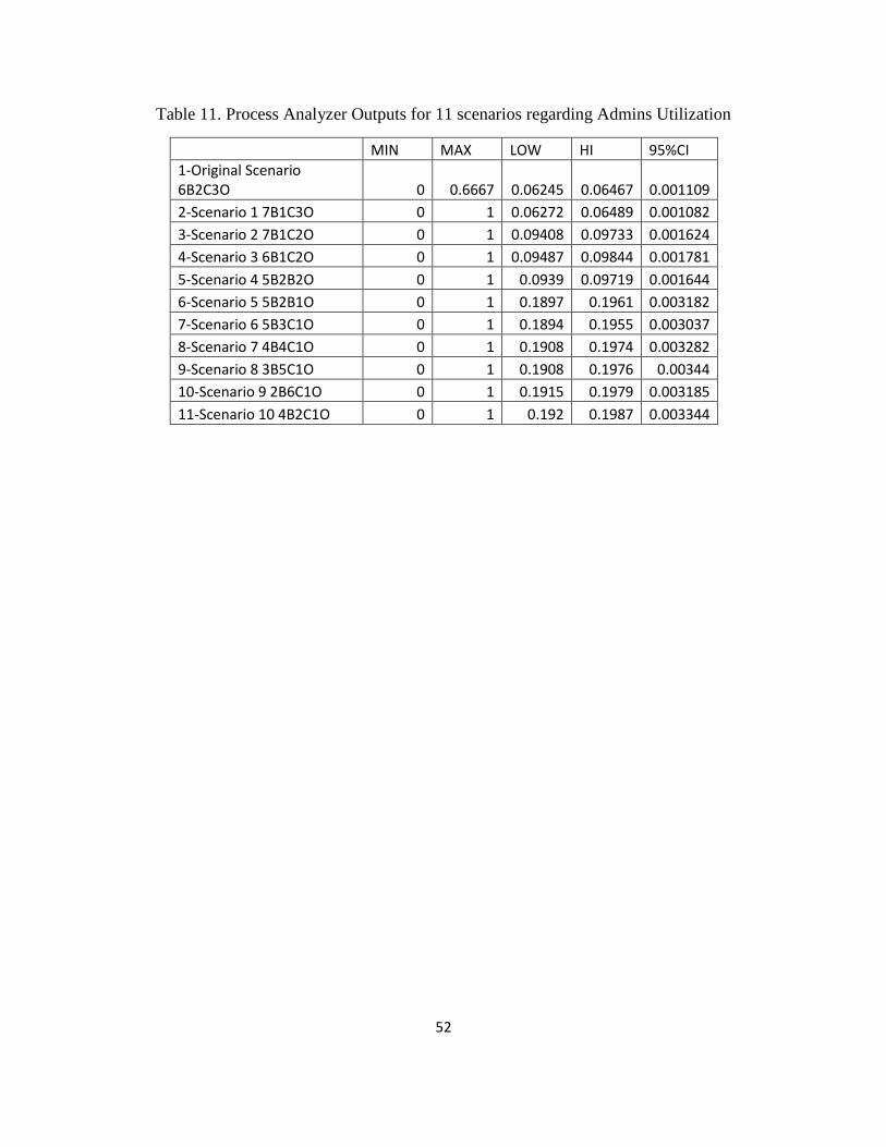
52

Table 11. Process Analyzer Outputs for 11 scenarios regarding Admins Utilization


1-Original Scenario 6B2C3O 0 0.6667 0.06245 0.06467 0.001109

2-Scenario 1 7B1C3O 0 1 0.06272 0.06489 0.001082

3-Scenario 2 7B1C2O 0 1 0.09408 0.09733 0.001624

4-Scenario 3 6B1C2O 0 1 0.09487 0.09844 0.001781

5-Scenario 4 5B2B2O 0 1 0.0939 0.09719 0.001644

6-Scenario 5 5B2B1O 0 1 0.1897 0.1961 0.003182

7-Scenario 6 5B3C1O 0 1 0.1894 0.1955 0.003037

8-Scenario 7 4B4C1O 0 1 0.1908 0.1974 0.003282

9-Scenario 8 3B5C1O 0 1 0.1908 0.1976 0.00344

10-Scenario 9 2B6C1O 0 1 0.1915 0.1979 0.003185

11-Scenario 10 4B2C1O 0 1 0.192 0.1987 0.003344

53

6. Conclusion and Recommendation

After the completion of the project, an efficient system was presented to the DRINKME

team to facilitate their operations in the long run. From the pilot study, we found that choosing a

mixed transportation delivery method could achieve a solution that accounts for both financial

and delivery time metrics. Also, by developing a simulation model, the team was able to

compare 11 scenarios and find the best scenario using sensitivity analysis. There are two best

scenarios. One came from pilot study, including 6 bikes and 2 cars with 3 administrative staff.

Another came from the simulation analysis, including 4 bikes and 4 cars with 1 administrative

staff. As a result of this project, we recommend this scenario as the best option because it

includes only 9 resources instead of the 11 in original scenario, which is a sign of a more

efficient system. However, improvements such as revising the back-stage system and database

system are recommended to DRINKME team to facilitate their overall operation in the long run.

If the company would like more quantitative analysis of the transportation options, an

optimization model is recommended.

6.1 The Preferred Solution

In order to illustrate the findings from the simulation, the team summarized all data from

scenario analysis by indicating with a “1” in the blank space corresponds to the response and

scenario ID to indicate the individually best results.

Table 12. Summary of Transportation Delivery Scenarios

Scenario ID Part3Time P1BTime P2 Car Bike Admin Total

Original Scenario 6B2C3O 1 1 1 3

Scenario 1 7B1C3O 1 1



Scenario 4 5B2B2O -

Scenario 5 5B2B1O 1 1 2

Scenario 6 5B3C1O 1 1 2

Scenario 7 4B4C1O 1 1 1 3


Scenario 9 2B6C1O 1 1 2


54

In Table 12, Part3Time means the travel time of type 3 orders; “P1BTime” means the travel time

of type 1 orders that placed from mobile app; “P2” means the travel time of type 2 orders. “Car”, “Bike”

and “Admin” in the table denotes the utilization of resources arranged in the scenario analysis. If there is

a “1” in the boxes, the attributes or resources listed with “1” achieved the best efficiency in the

corresponding scenario. Thus, more “1”s in a scenario means more efficiency. By looking at the

total grading for the 11 scenarios listed in our simulation, identify the scenarios with the most

significant results as the original scenario from the Pilot Study, along with scenario 7 in our

sensitively analysis.

Thus, the best arrangement for the transportation delivery could be 6 Bikes, 2 Cars with 3

Order Process Admins or 4 Bikes, 4 Cars and 1 Order Process Admins, which corresponds to the

original scenario and scenario 7, respectively. Both scenarios produce better results regarding

utilization of both resources and travel duration. If the company wants to maximize customer

satisfaction by minimizing delivery time, the original scenario settings are the best. However, if

the company want to emphasize efficiency more, scenario 7 would be recommended.

6.2 Future Improvements

This section introduces several future improvements that the DRINK team could

explore.

6.2.1 Revise the Back-Office Delivery System

In order to have the most efficient delivery rate, the company should revise the delivery

team’s back-office system to allow staff to operate the interface more easily, thus reducing

wasted time. Currently, after the pilot study, we found that the back-stage application on the

employee’s mobile phone was full of glitches that might produce mistakes and buggy quits,

which slowed down the order processing time.

55

6.2.2 Conduct an Optimization Objective Function

In order to maximize the efficiency of the resources, the solution provided by Arena

simulation might not be complete. An optimization model could be developed in order to yield

the number of resources that reduce costs and achieve reasonable travel times. In the simulation,

we tested specific choices, but not necessarily the best one. Thus, in order to produce a more

quantitative model that helps the company to figure out the most economic delivery method, an

optimization model in excel is in need.

6.2.3 Improve database systems

From our experience at DRINK-ME, we found that the database that contains the

historical sales data is hard to use due to discrepancy in units, lack of transparency about

information, and the misleading user interface. In our pilot study, we found that units are either

in a China scale or U.S scale, which is confusing while the driver or bike-rider tries to estimate

the time of arrival. Also, the system is unable to store the distance data, so we had to struggle to

analyze the data by calculating the distance based on coordinates information in the system. By

improving the database system, the company would produce a more efficient operation and

facilitate future data analysis.

6.2.4 Systematic Improvements/Recommendations from the Pilot Study

As we took a close look to the system after the three pilot study experiments, it is

interesting that we found some system imperfections that could be improved in the future. First,

the processing time for sending a driver is much longer than the time for notifying a bike rider.

Second, the system could be inefficient if there are many type III orders. During the pilot study,

we found out that on holidays or festivals, when type III orders escalated and the current

standard operating procedure for Type III orders was slow, causing a significant delay for

customers. The cars currently used are from the company’s own asset or from a rental company

upon request. All delivery vehicles in the first two scenarios are set at the permanent location at

first, and if no orders come in, the vehicles would not move. However, in the 3rd

test from the

pilot study, all vehicles were freely located due to the specific method we chose. Distributing

56

cars or bikes around might improve the delivery speed for the other pilot scenarios as well. Thus,

to be more efficient, the company should concentrate on improving the type III order delivery

rate and distribute cars so they are not at a permanent location.

6.3 Design Reflection

This section provides a reflection on the design in this project in an engineering design

context.

6.3.1 Design Concept

Upon completion of this project, a simulation model and a methodology, containing a process of

revising and improving DRINKME’s logistics system, has been explored and designed. First, an

assumption regarding potential improvements was made. Second, a pilot study was planned to

test potential solutions. Then, the team designed a simulation model that replicated the preferred

solution from pilot study. By controlling variables such as resources, the model created by the

team produced a preferred solution. The formation of this design emerged from the engineering

assumptions based on the background information, the insight provided by the team’s industrial

engineering background, and multiple trials to see what worked well. In the process of

developing a good solution, the team experienced a few challenges. First, we wanted to find a

specific number of total costs and compare them. However, the data we had and the simulation

model we created did not yield a very convincing answer for this objective. Thus, we finally

decided to focus on finding an overall improved system based on several important attributes like

number of resources used and total travel time. Meanwhile, an improved system has still been

developed based on the scenario and sensitivity analysis.

6.3.2 Constraints

The simulation model is not completely accurate. In the process of designing an Arena

model based on the pilot study and background information, for example, the team utilized the

DECIDE module’s two-way by chance features to simulate the rainy condition. However, the

reality of the operation for such an immediate service would rarely be what a DECIDE module

57

could replicate when it comes to the different standard operation procedure (SOP) for dealing

various incidents. Considering the short period of the project, the team decided not to explore a

more complicated way to simulate complex situations such as hazardous weather conditions,

special alcohol transportation, and mechanical failures or battery outrages of the delivery trunk.

The system in simulation model also does not consider other categorical factors such as the

traffic code in Shanghai and the seasonality of alcohol industry, which could influence the

delivery process.

The simulation model does not yield a straightforward financial outcome for different

scenarios. Because the simulation model was primarily designed to reflect the order delivery

time and the total costs involved not only travel time but also involved labor, sunk costs and

other complex variables, the operating costs then could not be easily produced upon completion

of each simulation. A more quantitative analysis based on costs could be developed using an

optimization model in Microsoft Excel.

The final recommendation, which involved using both types of transportation, could

results in greater difficulty in managing equipment maintenance, higher upfront costs for the

company and hiring requirements for delivery staff. The effect of increased difficulties in other

aspects of daily operation should be evaluated in the long run, in regards to the efficiency of the

whole company’s operation, liquidity, solvency, and depreciation of assets. Although the

solution is currently sustainable for the company, the long-term sustainability should be

questioned as China is a developing country where the technology and alcohol industry is

undergoing a dramatic revolution in 2016. Thus, the sustainability of the preferred solution

should be evaluated in the long run with the new policies, innovations and technology.

Despite the constraints above, the team was able to find an improved system resulting in

18% savings in resources and approximately 10% savings in total delivery time for the company.

Furthermore, the simulation model identifies where issues exist under different settings and the

management team examine how simulation results vary to adjust the standard operating

procedure (SOP) of the delivery process. Although the team did not focus on how much exactly

the system cost because of short project time, a resource-based results could also explain which

scenario is significantly better financially.

58

6.4 Lifelong Learning Reflection

By completing the project, the author strengthened his insight about how to solve

industrial engineering problems, gained knowledge of how to make decision to optimize the

system and examined the nature of engineering design. During the pilot study and model

simulation, the author made several observations and reflections on the industrial engineering

endeavor in the real business world.

The back-office system design is equally important as the user-interface of the

application. Based on the pilot study, the inconvenience of operating the back-office system

stood out as a potential factor delaying the delivery. Before this project, the author regarded the

user interface as the most important feature of a successful product and it was tolerable to have

an average but unexceptional design of the back-office system. However, after this project, the

author discovered that a tiny design flaw in the back-office system could contribute to the

difficulties of daily operations, human resources management and low customer satisfaction. For

example, the design of back-office system at DRINKME does not adopt industrially-preferred

check-box confirmation for each item in the order. Instead, it only informed the delivery person

of the total amount of bottles for each item in the order, which increased the possibility of human

error. Such human error could decrease the efficiency of the logistics system indirectly and lower

customer satisfaction the wrong items were picked up. Thus, the author concluded that a

successful design of a back-office system could also be beneficial to improved efficiency.

It is important to make a give-up decision when designing the simulation n model.

During the process of creating simulation model, the team considered too much factors which

delayed the project progress by stagnating the simulation process. However, after leaving out

some of less influential variables, the simulation works and produces a meaningful result for

improvement. In the future of my industrial engineering career, whenever I met a dilemma in

simulation problems and could not solve it in a short period, it would remind me of this project

experience that one could get rid of some factors and let the system run first, and then try adding

more elements back with the development of the model.

59

There is no end for optimization. The final recommendation proposes use of 4 bikes, 4

cars and 1 administrator, which would reduce the number of resources from 11 to 9. However,

the increasing use of cars could increase the risk of financial problems. Besides, with the

increased number of orders provided by the expansion in Shanghai, management of a delivery

fleet composed of two types of transportation could be more challenging. Moreover, the

management, maintenance, and training for the delivery team could face additional challenges in

the long run. There is no real permanent best solution in the industrial engineering field. This

project demonstrated that a system, once introduced, can always be improved in some aspects.

And some improvements bring inconvenience to other aspects. Although the optimization

process could be endless, the author reflects that what the decision-maker values most is a

compromise solution.

60

References

DRINKME | Your Private Butler. (n.d.). Retrieved December/January, 2015, from

http://drinkme.org/

Discrete Event Simulation Software | Manufacturing, Supply Chain & Healthcare

Simulation Software | Arena Simulation. (n.d.). Retrieved December 12, 2015, from

https://www.arenasimulation.com/

Excel Solver Help. (n.d.). Retrieved December 12, 2015, from

http://www.solver.com/excel-solver-help

Fan, W., Xu, H., & Xu, X. (2009). Simulation on vehicle routing problems in logistics

distribution. COMPEL - The International Journal for Computation and Mathematics in

Electrical and Electronic Engineering, 1516-1531.

Gevaers, R., Voorde, E., & Vane slander, T. (n.d.). Characteristics and Typology of Last-

mile Logistics from an Innovation Perspective in an Urban Context. City Distribution and

Urban Freight Transport.

Lee, H., & Whang, S. (2001, July 1). Winning the Last Mile of E-Commerce. Retrieved

December 6, 2015, from http://sloanreview.mit.edu/article/winning-the-last-mile-of-

ecommerce/

Lee, H., & Anderson, D. (n.d.). The Internet-Enabled Supply Chain: From the “First

Click” to the “Last Mile”. Retrieved December 9, 2015, from

ftp://ftp.gunadarma.ac.id/idkf/www.bogor.net/www.bogor.net/idkf-wireless/aplikasi/e-

commerce/anderson-d.pdf

Mentzer, J. T., & Konrad, B. P. (1991). An Efficiency/Effectiveness approach to logistics

performance analysis. Journal of Business Logistics, 12(1), 33. Retrieved from

http://ezproxy.wpi.edu/login?url=http://search.proquest.com/docview/212660593?accoun

tid=29120

Radulescu, Alexandru Valentin, and Radu Mircea Carp Ciocardia. "Simulation of the

information flow and supply chain using arena modelling software." Annals of DAAAM

& Proceedings (2009): 445+. Academic OneFile. Web. 13 Dec. 2015.

61

Soper, T. (2014, November 1). Quick liquor: Alcohol delivery service Drizly launches in

Seattle - GeekWire. Retrieved December 22, 2015, from

http://www.geekwire.com/2014/need-booze-quick-alcohol-delivery-service-drizly-

launches-seattle/

Y., M. (n.d.). Simulation-Based Case Studies in Logistics.

improving delivery efficiency and effectiveness for the ... · improving delivery efficiency and...

Documents