improving forensic identification using bayesian networks and relatedness estimation
TRANSCRIPT

The author(s) shown below used Federal funds provided by the U.S. Department of Justice and prepared the following final report: Document Title: Improving Forensic Identification Using
Bayesian Networks and Relatedness Estimation: Allowing for Population Substructure
Author: Amanda B. Hepler Document No.: 231831
Date Received: September 2010 Award Number: 2004-DN-BX-K006 This report has not been published by the U.S. Department of Justice. To provide better customer service, NCJRS has made this Federally-funded grant final report available electronically in addition to traditional paper copies.
Opinions or points of view expressed are those
of the author(s) and do not necessarily reflect the official position or policies of the U.S.
Department of Justice.
Abstract
Hepler, Amanda Barbara. Improving Forensic Identification Using Bayesian Networks
and Relatedness Estimation: Allowing for Population Substructure (Under the direc-
tion of Bruce S. Weir.)
Population substructure refers to any population that does not randomly mate. In
most species, this deviation from random mating is due to emergence of subpopulations.
Members of these subpopulations mate within their subpopulation, leading to different
genetic properties. In light of recent studies on the potential impacts of ignoring these
differences, we examine how to account for population substructure in both Bayesian
Networks and relatedness estimation.
Bayesian Networks are gaining popularity as a graphical tool to communicate com-
plex probabilistic reasoning required in the evaluation of DNA evidence. This study
extends the current use of Bayesian Networks by incorporating the potential effects
of population substructure on paternity calculations. Features of HUGIN (a software
package used to create Bayesian Networks) are demonstrated that have not, as yet,
been explored. We consider three paternity examples; a simple case with two alleles, a
simple case with multiple alleles, and a missing father case.
Population substructure also has an impact on pairwise relatedness estimation. The
amount of relatedness between two individuals has been widely studied across many
scientific disciplines. There are several cases where accurate estimates of relatedness
are of forensic importance. Many estimators have been proposed over the years, how-
ever few appropriately account for population substructure. New maximum likelihood
estimators of pairwise relatedness are presented. In addition, novel methods for re-
lationship classification are derived. Simulation studies compare these estimators to
those that do not account for population substructure. The final chapter provides real
data examples demonstrating the advantages of these new methodologies.
This document is a research report submitted to the U.S. Department of Justice. This report has not been published by the Department. Opinions or points of view expressed are those of the author(s) and do not necessarily reflect the official position or policies of the U.S. Department of Justice.
Improving Forensic Identification Using BayesianNetworks and Relatedness Estimation: Allowing
for Population Substructure
by
Amanda B. Hepler
a dissertation submitted to the graduate faculty of
north carolina state university
in partial fulfillment of the
requirements for the degree of
doctor of philosophy
department of statistics
raleigh
August 15, 2005
approved by:
Dr. Bruce Weir (Chair) Dr. Jacqueline Hughes-Oliver
Dr. Maria Oliver-Hoyo Dr. Jung-Ying Tzeng
This document is a research report submitted to the U.S. Department of Justice. This report has not been published by the Department. Opinions or points of view expressed are those of the author(s) and do not necessarily reflect the official position or policies of the U.S. Department of Justice.

Dedication
To Carol and Ernest Hepler.
ii
This document is a research report submitted to the U.S. Department of Justice. This report has not been published by the Department. Opinions or points of view expressed are those of the author(s) and do not necessarily reflect the official position or policies of the U.S. Department of Justice.

Biography
Amanda Hepler was born on July 26, 1977, in Frankfurt, Germany. Because her father
was a career Army officer she had an opportunity to travel extensively and live in
many places including Germany, Texas, Virginia, Florida, and Maryland. During her
vacations with her family she visited over fifteen European countries and developed a
love for traveling.
In 1995, Amanda graduated from Fallston High School, in Fallston Maryland. She
attended the University of Central Florida for her first year of undergraduate stud-
ies. Amanda returned to Maryland to continue her education at Towson University
majoring in applied mathematics and computing. During her undergraduate program,
Amanda was nominated by professors within the Mathematics Department for hon-
orary membership in the Association for Women in Mathematics. She received the
Mary Hudson Scarborough Honorable Mention for Excellence in Mathematics during
her final year at Towson and graduated summa cum laude in 2001.
Amanda selected North Carolina State University for graduate school where she
received her Masters in Statistics in 2003. During her masters’ program she was nom-
inated for membership in the Phi Kappa Phi Honor Society and Mu Sigma Rho, a
National Statistics Honor Society. Amanda worked for two years as a research as-
sistant for the Office of Assessment performing various statistical analyses under the
direction of Dr. Marilee Bresciani. During her 2003 spring semester, she began re-
searching Bayesian Networks under the direction of Bruce Weir. Amanda was formally
accepted into the statistics doctoral program in the fall of 2003. Dr. Weir continued
to guide her research during her doctoral studies. Amanda finished the requirements
for her doctoral degree in August, 2005, and is currently working with Dr. Weir as a
post-doctoral student.
iii
This document is a research report submitted to the U.S. Department of Justice. This report has not been published by the Department. Opinions or points of view expressed are those of the author(s) and do not necessarily reflect the official position or policies of the U.S. Department of Justice.

Acknowledgements
This research was supported by a graduate research grant from the National Institute
of Justice. Additional funding was provided by the NCSU Department of Statistics.
Office space, computing equipment, travel funding, and a superb staff were supplied
by the Bioinformatics Research Center. Bruce Weir, Jacqueline Hughes-Oliver, Maria
Oliver-Hoyo and Jung-Ying Tzeng all provided insightful comments, greatly improving
the quality of this dissertation. Additional improvements were suggested by Ernest
Hepler and Clay Barker.
Dr. Bruce Weir provided me with the tremendous opportunity of working with him
during the past few years. His guidance has been invaluable and it is an honor to have
been selected as one of his students. No doctoral student could have a better mentor
and advisor. It has truly been a pleasure.
There have certainly been others who have influenced me during this long aca-
demic journey. I began as a struggling speech pathology student at Towson University.
Dr. Diana Emanuel, a hearing science professor, was the first to suggest I take a few
math courses. A former psychology professor, Dr. Arthur Mueller, provided a brilliant
introduction to the world of statistics. His enthusiasm and passion for the field started
me on this path. Dr. Bill Swallow, a statistics professor at NCSU encouraged me to
explore forensic research opportunities with Dr. Weir. These professors marked my
path at critical decision points and made it possible for me to be here today.
There have been long sleepless nights torturing over homework, much academic
confusion, misery, and wishes for the end. Survival was due to the willingness of my
closest friends to be tortured beside and by me. My eternal gratitude is given to Aarthi,
Clay, Darryl, Donna, Eric, Frank, Harry, Joe, Jyotsna, Kirsten, Lavanya, Marti, Matt,
Michael, Mike, Paul, Ray, and Theresa. Basketball games, Friday’s at Mitch’s, and
iv
This document is a research report submitted to the U.S. Department of Justice. This report has not been published by the Department. Opinions or points of view expressed are those of the author(s) and do not necessarily reflect the official position or policies of the U.S. Department of Justice.

hours and hours of playing pool with the best of friends made this experience bear-
able...almost enjoyable. There are others who have who have encouraged and supported
me through this experience. David, Lisa and Laura have given me endless love and
support. My three loving grandparents have never been shy in saying how proud they
are of me. Their faith and encouragement are a constant source of inspiration. I would
also like to thank Joel, who has been by my side and endured all the emotional “ups
and downs” of this last year. He has helped me stay focused and encouraged me every
step of the way. I only hope I can do half the job he’s done when it’s my turn.
Last, and certainly not least, there is the profound influence of my parents, Carol
and Ernie Hepler. Throughout my life, they provided an environment rich in support,
guidance, patience and most importantly, love. I am in awe every day of the things
they have both accomplished, and are continuing to strive towards. My father’s vision,
integrity, and ambition have inspired me all my life. In my eyes, my mother has attained
excellence in every aspect of her career, all along keeping it in perfect balance with her
family and friends. As I embark on my own career, I am blessed to have her example
to follow. My parents have always been in my corner, believing in me, encouraging me
to try things I never thought were possible. Their love (not to mention great genes)
are the foundation for my success. Thank you both!
v
This document is a research report submitted to the U.S. Department of Justice. This report has not been published by the Department. Opinions or points of view expressed are those of the author(s) and do not necessarily reflect the official position or policies of the U.S. Department of Justice.
Table of Contents
List of Tables viii
List of Figures x
1 Bayesian Networks and Population Substructure 1
1.1 Introduction . . . . . . . . . . . . . . . . . . . . . . . . . . . . . . . . . 1
1.2 Review of Relevant Literature . . . . . . . . . . . . . . . . . . . . . . . 3
1.3 Research Methods . . . . . . . . . . . . . . . . . . . . . . . . . . . . . . 7
1.4 Example One: A Simple Paternity Case with Two Alleles . . . . . . . . 9
1.5 Example Two: A Simple Paternity Case with Multiple Alleles . . . . . 18
1.6 Example Three: A Complex Paternity Case with Two Alleles . . . . . . 22
1.7 Discussion . . . . . . . . . . . . . . . . . . . . . . . . . . . . . . . . . . 26
2 Pairwise Relatedness and Population Substructure 27
2.1 Introduction . . . . . . . . . . . . . . . . . . . . . . . . . . . . . . . . . 27
2.2 Review of Relevant Literature . . . . . . . . . . . . . . . . . . . . . . . 31
2.3 Research Methods . . . . . . . . . . . . . . . . . . . . . . . . . . . . . . 44
2.4 Results . . . . . . . . . . . . . . . . . . . . . . . . . . . . . . . . . . . . 55
2.5 Discussion . . . . . . . . . . . . . . . . . . . . . . . . . . . . . . . . . . 64
3 Applications to Real Data 65
3.1 Introduction . . . . . . . . . . . . . . . . . . . . . . . . . . . . . . . . . 65
3.2 Pairwise Relatedness Estimation . . . . . . . . . . . . . . . . . . . . . . 66
3.3 Multiple Allele Paternity Network Example . . . . . . . . . . . . . . . 83
3.4 Discussion . . . . . . . . . . . . . . . . . . . . . . . . . . . . . . . . . . 85
Literature Cited 86
vi
This document is a research report submitted to the U.S. Department of Justice. This report has not been published by the Department. Opinions or points of view expressed are those of the author(s) and do not necessarily reflect the official position or policies of the U.S. Department of Justice.
Appendices 90
A A Simple Bayesian Network 91
B Corrections and Comments on Wang’s Paper [1] 98
C Downhill Simplex Method C++ Code 100
C.1 C++ Function Obtaining 8D MLE . . . . . . . . . . . . . . . . . . . . 100
C.2 Simplex Class C++ Header File . . . . . . . . . . . . . . . . . . . . . . 101
C.3 Simplex Class C++ Implementation File . . . . . . . . . . . . . . . . . 101
C.4 Likelihood Class C++ Header File . . . . . . . . . . . . . . . . . . . . 109
C.5 Likelihood Class C++ Implementation File . . . . . . . . . . . . . . . . 109
D Summary of Loci from CEPH Families 115
vii
This document is a research report submitted to the U.S. Department of Justice. This report has not been published by the Department. Opinions or points of view expressed are those of the author(s) and do not necessarily reflect the official position or policies of the U.S. Department of Justice.

List of Tables
1.1 Algebraic Pi Values for Founder3 using Equation 1.6. . . . . . . . . . . 8
1.2 Numerical Pi Values for Founder3 using Equation 1.6. . . . . . . . . . 9
1.3 Notation for Putative Father, Mother and Child Nodes. . . . . . . . . . 11
1.4 Paternity Index Formulas Derived in [2]. . . . . . . . . . . . . . . . . . 17
1.5 Notation for Network in Figure 1.13. . . . . . . . . . . . . . . . . . . . 23
2.1 Common θXY Values. . . . . . . . . . . . . . . . . . . . . . . . . . . . . 29
2.2 Similarity Index (SXY ) Values for All IBS Patterns. . . . . . . . . . . . 34
2.3 Conditional Probabilities Pr(λi|Sj), with No Population Substructure. . 39
2.4 Conditional Probabilities Pr(λi|Sj), with Population Substructure. . . . 42
2.5 Relationships Among Various Relateness Coefficients. . . . . . . . . . . 50
2.6 Conditional Probabilities based on Seven Parameters. . . . . . . . . . . 50
2.7 Jacquard’s Coefficients in Terms of the Inbreeding Coefficient (ψ) for
Some Common Relationships. . . . . . . . . . . . . . . . . . . . . . . . 53
2.8 Jacquard’s True Parameter Values for Full Siblings. . . . . . . . . . . . 53
2.9 MLE, True ∆ Vectors, and Euclidean Distances for Example in Section 2.3. 54
2.10 Simulated Accuracy Rates for the Distance Metric Classification Methods. 62
3.1 2D, 6D and 8D MLEs, Bootstrap (BS) Standard Errors and 90% BS CIs. 68
3.2 Biases and Standard Errors for the 2D and 8D MLEs, FBI Data. . . . . 75
3.3 Individual Accuracy Rates for FBI Data. . . . . . . . . . . . . . . . . . 77
3.4 Standard Errors of the 2D, 6D and 8D MLE for Selected Samples. . . . 79
3.5 Individual Accuracy Rates for HapMap Data. . . . . . . . . . . . . . . 81
3.6 CEPH Family 102 Genotypes and PI Values. . . . . . . . . . . . . . . . 84
A.1 Unconditional Probability Table for Guilty Node. . . . . . . . . . . . . 93
viii
This document is a research report submitted to the U.S. Department of Justice. This report has not been published by the Department. Opinions or points of view expressed are those of the author(s) and do not necessarily reflect the official position or policies of the U.S. Department of Justice.

A.2 Conditional Probability Table for True Match Node. . . . . . . . . . . 94
A.3 Conditional Probability Table for Reported Match Node. . . . . . . . 94
B.1 Mistaken Probabilities in Wang [1]. . . . . . . . . . . . . . . . . . . . . 99
D.1 CEPH Family Locus Numbers, Names, and Chromosome Locations. . . 115
D.2 Allele Frequencies for CEPH Loci Defined in Table D.1. . . . . . . . . . 116
ix
This document is a research report submitted to the U.S. Department of Justice. This report has not been published by the Department. Opinions or points of view expressed are those of the author(s) and do not necessarily reflect the official position or policies of the U.S. Department of Justice.

List of Figures
1.1 Putative Father’s Node Trio. . . . . . . . . . . . . . . . . . . . . . . . . 10
1.2 Probability Table for Putative Father’s Paternal Gene Node. . . . . . . 10
1.3 Conditional Probability Table for Putative Father’s Genotype Node. . . 11
1.4 Network for Hypothesis, True Father and Putative Father Nodes. . . . 12
1.5 Conditional Probability Table for True Father’s Paternal Gene Node. . 12
1.6 Simple Paternity Network from Dawid et al. [3]. . . . . . . . . . . . . . 13
1.7 Population Substructure Simple Paternity Network. . . . . . . . . . . . 14
1.8 Conditional Probability Table for Mother’s Paternal Gene. . . . . . . . 15
1.9 Probability Tables for Counting Nodes. . . . . . . . . . . . . . . . . . . 16
1.10 HUGIN’s Output After Entering the Evidence, Simple Paternity Network. 17
1.11 Population Substructure Paternity Network for Multiple Alleles. . . . . 19
1.12 HUGIN’s Output After Entering the Evidence, Multiple Allele Network. 21
1.13 Complex Paternity Network. . . . . . . . . . . . . . . . . . . . . . . . . 23
1.14 Population Substructure Complex Paternity Network. . . . . . . . . . . 24
1.15 HUGIN’s Output After Entering the Evidence, Complex Paternity Net-
work. . . . . . . . . . . . . . . . . . . . . . . . . . . . . . . . . . . . . . 25
2.1 Diagram of IBD Relationship Between Two Siblings X and Y . . . . . . 28
2.2 IBD Patterns Between Two Individuals, for the Non-Inbred Case. . . . 30
2.3 IBD Patterns Between Two Individuals, for the Inbred Case. . . . . . . 42
2.4 Graph of Likelihood Function. . . . . . . . . . . . . . . . . . . . . . . . 47
2.5 Graph of Likelihood Function with Intercepting Plane. . . . . . . . . . 47
2.6 IBD Patterns Between Two Individuals, for the Seven Parameter Inbred
Case. . . . . . . . . . . . . . . . . . . . . . . . . . . . . . . . . . . . . . 49
2.7 Means Plots for 2D MLE, Based on 500 Simulated Data Points per Plot. 56
x
This document is a research report submitted to the U.S. Department of Justice. This report has not been published by the Department. Opinions or points of view expressed are those of the author(s) and do not necessarily reflect the official position or policies of the U.S. Department of Justice.

2.8 Means Plots for 8D MLE, Based on 500 Simulated Data Points per Plot. 57
2.9 Plots of the Bias for 2D, 6D, and 8D MLEs, Based on 500 Simulated
Data Points per Plot, Ten Alleles per Locus. . . . . . . . . . . . . . . . 58
2.10 Standard Deviations for 2D MLE, Based on 500 Simulated Data Points
per Plot. . . . . . . . . . . . . . . . . . . . . . . . . . . . . . . . . . . . 59
2.11 Standard Deviations for 8D MLE, Based on 500 Simulated Data Points
per Plot. . . . . . . . . . . . . . . . . . . . . . . . . . . . . . . . . . . . 60
2.12 Plots of the Standard Deviations for 2D, 6D, and 8D MLEs, Based on
500 Simulated Data Points per Plot, Ten Alleles per Locus. . . . . . . . 61
2.13 Accuracy Rates for 2D Method, Based on 500 Simulated Data Points
per Plot. . . . . . . . . . . . . . . . . . . . . . . . . . . . . . . . . . . . 63
3.1 Representative CEPH Family Pedigree. . . . . . . . . . . . . . . . . . . 66
3.2 2D, 6D and 8D MLEs for Unrelated CEPH Individuals, based on 20 or
50 loci. . . . . . . . . . . . . . . . . . . . . . . . . . . . . . . . . . . . . 67
3.3 P0 versus P1 Plots for Unrelated CEPH Individuals. . . . . . . . . . . . 69
3.4 2D, 6D and 8D MLEs for Full Sibling and Parent Child CEPH Pairs . 70
3.5 CEPH Data Accuracy Rates for 2D, 6D and 8D Discrete Relatedness
Estimates. . . . . . . . . . . . . . . . . . . . . . . . . . . . . . . . . . . 72
3.6 Plotted Biases of the 2D, 6D and 8D MLEs, FBI Data. . . . . . . . . . 74
3.7 Plotted Standard Deviations of the 2D, 6D and 8D MLEs, FBI Data. . 74
3.8 P0 versus P1 Plots for Simulated Parent-Child Pairs from AA Sample. . 76
3.9 Mean Accuracy Rates for FBI Data. . . . . . . . . . . . . . . . . . . . 77
3.10 Plotted Biases of the 2D and 8D MLEs, HapMap Data. . . . . . . . . . 79
3.11 Mean Accuracy Rates for Hapmap Data. . . . . . . . . . . . . . . . . . 80
3.12 P0 versus P1 Plots for Simulated Pairs from CEU Sample. . . . . . . . 81
3.13 Classification Rates for the 8D Method when True Relationship is Full
Sibling. . . . . . . . . . . . . . . . . . . . . . . . . . . . . . . . . . . . . 82
A.1 A Simple Bayesian Network. . . . . . . . . . . . . . . . . . . . . . . . . 92
xi
This document is a research report submitted to the U.S. Department of Justice. This report has not been published by the Department. Opinions or points of view expressed are those of the author(s) and do not necessarily reflect the official position or policies of the U.S. Department of Justice.

A.2 Probability Tables from HUGIN. . . . . . . . . . . . . . . . . . . . . . 95
A.3 Before Entering the Evidence. . . . . . . . . . . . . . . . . . . . . . . . 96
A.4 After Entering the Evidence that we have a Reported Match. . . . . 97
xii
This document is a research report submitted to the U.S. Department of Justice. This report has not been published by the Department. Opinions or points of view expressed are those of the author(s) and do not necessarily reflect the official position or policies of the U.S. Department of Justice.

Chapter 1
Bayesian Networks and Population
Substructure
1.1 Introduction
Population Substructure Effects on Forensic Calculations
One method of evaluating a body of evidence is to calculate a likelihood ratio [4]. This
is a ratio of two probabilities:
LR =Pr(Evidence given the prosecutor’s hypothesis)
Pr(Evidence given the defendant’s hypotheses). (1.1)
Generally, the defense’s hypothesis is that the evidence profile reflects someone other
than the defendant. The prosecution, in contrast, argues that the match between the
evidence profile and the defendant’s profile means that the defendant was the source of
the evidence. The denominator of this likelihood ratio requires that a forensic scientist
determine the probability of observing the same DNA profile twice, commonly referred
to as the match probability [2]. The numerator is typically 1, as the prosecutor is
proposing that the evidence points to the defendant. In this case, the likelihood ratio
reduces to the inverse of the match probability. Likelihood ratios can take on values
from 0 to ∞. If we obtain a value of 100 for our ratio, the common interpretation is
“The evidence is 100 times more probable if the suspect left the evidence than if some
unknown person left the evidence” [2].
When population substructure is ignored, the match probability is simply the rela-
tive frequency of the defendant’s profile in the suspected population of the culprit [5].
Essentially, this treats each human population as large and randomly mating, ignoring
1
This document is a research report submitted to the U.S. Department of Justice. This report has not been published by the Department. Opinions or points of view expressed are those of the author(s) and do not necessarily reflect the official position or policies of the U.S. Department of Justice.

Chapter 1. Bayesian Networks and Population Substructure
possible subpopulations. People in these subpopulations could tend to mate within
their subpopulation which would lead to different allelic frequencies than those esti-
mated from the overall population. To estimate these possible differences, it is nec-
essary to introduce a measure of background relatedness among the subpopulations
under consideration. This term, typically denoted θ, is commonly referred to as the
inbreeding coefficient [4]. In 1994, Balding and Nichols proposed a method for calcu-
lating match probabilities, which makes use of this inbreeding coefficient [6]. We use
this methodology here, and it is further examined in Sections 1.2 and 1.3.
Bayesian Networks in Forensics
Likelihood ratios can be calculated rather simply using Bayesian Networks (also known
as Probabilistic Expert Systems or Bayesian Belief Networks). A Bayesian Network
(BN) is a graphical and numerical representation which enables us to reason about
uncertainty. Contrary to the name, BNs are not dependent upon Bayesian reasoning.
In fact, the methods and assumptions we use in this research are not Bayesian in
nature, we appeal only to Bayes Theorem and probability calculus. BNs are simply a
tool to make the implications of complex probability calculations clear to the layperson,
without requiring an understanding of the complexity involved [7]. They provide an
automated way to calculate likelihood ratios in cases where the calculations are quite
laborious to perform analytically.
The use of BNs for forensic calculations has been gaining popularity over the past
decade due to the development of several software packages available which make the
construction of these networks relatively simple. These packages include HUGIN1
(which is used in this study), XBAIES2, Genie3, WINBUGS4, and most recently
FINEX5 [8]. A detailed discussion of BNs and their applications can be found in [9],
1Free evaluation version available at http://www.hugin.dk2Free to the public, available at http://www.staff.city.ac.uk/∼rgc3Available at http://www2.sis.pitt.edu/∼genie4Free to the public, available at http://www.mrc-bsu.cam.ac.uk/bugs/winbugs/contents.shtml5Not yet available to the public, for updates see http://www.staff.city.ac.uk/∼rgc
2
This document is a research report submitted to the U.S. Department of Justice. This report has not been published by the Department. Opinions or points of view expressed are those of the author(s) and do not necessarily reflect the official position or policies of the U.S. Department of Justice.

Chapter 1. Bayesian Networks and Population Substructure
however a brief introduction is presented in Appendix A.
In this study extensive use is made of a table generating feature of HUGIN Version
6.3. This feature allows the use of general formulas for probability tables and avoids
the need to enter each probability by hand. The use of this feature should significantly
reduce data entry time which historically has been one of the major complaints in using
BN software.
1.2 Review of Relevant Literature
The examination of DNA evidence has become important to legal systems throughout
the world. Because of this, considerable research has focused on the validity and
reliability of current methods used to evaluate DNA. Two aspects of this research are
reviewed. First, the current state of forensic research concerning DNA calculations,
when accounting for population substructure, is summarized. It is also important to
critically examine the contributions of research using Bayesian Networks to answer
relevant questions in this forensic area.
Effects of Population Substructure
Incorporating population substructure in the evaluation of DNA profile evidence is
relatively recent. Several researchers, including Balding and Nichols [6, 5] and Weir
et al. [10, 11, 4], have pioneered examining the impact of population substructure on
DNA evidence evaluation. In 1995, Balding and Nichols conclude ignoring population
substructure “would unfairly overstate the strength of the evidence against the de-
fendant and the error could be crucial in some cases, such as those involving partial
profiles or large numbers of possible culprits, many of whom share the defendant’s
ethnic background” [5]. In this review, we demonstrate the detrimental effects of ig-
noring population substructure when evaluating DNA evidence. Balding and Nichols’
approach for accounting for population substructure is also reviewed.
3
This document is a research report submitted to the U.S. Department of Justice. This report has not been published by the Department. Opinions or points of view expressed are those of the author(s) and do not necessarily reflect the official position or policies of the U.S. Department of Justice.

Chapter 1. Bayesian Networks and Population Substructure
In 1994, Weir calculated estimates of the inbreeding coefficient, θ, using data ob-
tained from the Arizona Department of Public Safety on Native American, Hispanic,
African American, and Caucasian populations [11]. Weir showed a tenfold increase
in θ values for the Native American sample, relative to the other samples considered.
These estimates for θ ranged from 0.001 up to 0.097. Weir also demonstrated the
potential impacts of using a subpopulation with a high background relatedness factor.
For example, when assuming θ = 0, and an allele frequency of 0.05, the likelihood
ratio obtained is 200. However, if the true value of θ was actually 0.05, the likeli-
hood ratio obtained is 58. According to Evett and Weir [2], these two values could be
communicated as “moderate support” (LR=58) versus “strong support.” These two
interpretations could have quite a large impact when presented to a jury, and Weir’s
study demonstrates that the effects of population substructure need to be taken into
account when evaluating DNA evidence.
A relatively simple method of taking population substructure into account while
investigating DNA evidence was proposed by Balding and Nichols in 1994. This method
is being used in some UK courts and has been endorsed by several researchers [4, 12,
13]. As mentioned earlier, to calculate a likelihood ratio in a DNA evidence case
one needs to determine the match probability. Balding and Nichols proposed that
these calculations need to take into account all other observed alleles, whether taken
from the suspect or not. For example, suppose we are considering a paternity case in
which we have the genotypes for the mother, child, putative (alleged) father, as well
as both of the mother’s parents. In this case, Balding and Nichols propose that the
probability the putative father’s genotype matches the true father’s varies based on
the observed genotypes of all others involved. The actual formula used is presented in
Section 1.3. Their derivation of this formula depends upon the assumptions that they
have a “randomly-mating subpopulation partially isolated from a large population,
in which migration and mutation events occur independently and at constant rates.”
They provide both a genetical derivation and a statistical derivation of this formula.
In conclusion, Balding and Nichols claim the “proposed method captures the primary
4
This document is a research report submitted to the U.S. Department of Justice. This report has not been published by the Department. Opinions or points of view expressed are those of the author(s) and do not necessarily reflect the official position or policies of the U.S. Department of Justice.

Chapter 1. Bayesian Networks and Population Substructure
effects [of population substructure] and other sources of uncertainty” [6].
The 1996 National Research Committee (NRC) report discussed the most appro-
priate way of accounting for population substructure when evaluating DNA evidence.
They concluded in Recommendation 4.2 that “if the allele frequencies for the subgroup
are not available, although data for the full population are, then the calculations should
use the population-structure equations [derived by Balding and Nichols]” [14]. In light
of this recommendation, and due to the simple nature of Balding and Nichols’ method,
it is used to calculate all match probabilities in this research.
In summary, the cited research demonstrates the impact of population substruc-
ture on the evaluation of DNA evidence. The chance of this background relatedness
occurring in certain populations is large, and ignoring this potential could lead to er-
rors in probability calculations. It seems reasonable that there is a higher amount
of background relatedness among many populations, in addition to those discussed in
Weir’s 1994 article. Several cultures throughout the United States have a high oc-
currence of inbreeding, which speaks to the importance of ongoing research in this
area. Today, DNA evidence is used routinely by courts to establish guilt or innocence.
Population substructure must be considered or the credibility of this evidentiary tool
could be called into question. Balding and Nichols have proposed a method of taking
into account population substructure when evaluating DNA evidence. This method-
ology provides a simple, effective way to incorporate population substructure into our
Bayesian Network.
Bayesian Networks in Forensics
Bayesian Networks are gaining popularity in the forensic sciences as a tool to graph-
ically represent the complexities that arise in evaluating various types of evidence.
These networks provide a means of performing calculations that are very involved,
generally requiring extensive understanding of probability calculus. Bayesian Net-
works help scientists “follow a logical framework in complex situations” and “aid in
5
This document is a research report submitted to the U.S. Department of Justice. This report has not been published by the Department. Opinions or points of view expressed are those of the author(s) and do not necessarily reflect the official position or policies of the U.S. Department of Justice.

Chapter 1. Bayesian Networks and Population Substructure
constructing legal arguments” [15, 13]. Recently, Evett et al. claimed that BNs will
play an increasingly important role in forensic science and that their power lies in “en-
abling the scientist to understand the fundamental issues in a case and to discuss them
with colleagues and advocates [which] is something that has not been previously seen
in forensic science” [16].
Researchers have examined a wide array of forensic cases over the past few years
with the aid of BNs, ranging from simple car accident scenarios [17] to a highly com-
plex murder case [15]. Other researchers have explored using BNs to model the most
complex DNA evidence cases. The cases that have been examined to date are quite
exhaustive and include: paternity determination [3, 8], taking into account muta-
tion [3, 18], small quantities of DNA [16], cross-transfer evidence [19], and mixture
cases with partial profiles involved [20, 21, 8].
Considering the importance of DNA evaluation to our legal system, further research
into using Bayesian Networks seems prudent. Their graphical representations provide
a vehicle for communication between practitioners when discussing very complex cases.
They reduce the amount of confusion that can occur, by presenting important rela-
tionships between evidence in a logical way. No calculations are required to use these
networks, which is a major benefit to the forensic scientist. In addition, once a net-
work has been created, it can be used repeatedly in similar cases. For DNA evidence
cases, the only modification needed is the specification of allele frequencies, inbreeding
coefficient, and evidentiary profiles, as these values change from case to case. BNs
are fulfilling a need in the forensic community, and this study intends to explore their
usefulness in a wider array of cases. To date, BN studies have not taken into account
the impact that population substructure may have on final DNA analysis. This study
examines various DNA profile cases using BNs and explores potential improvements
that can be made in DNA examination by considering population substructure.
6
This document is a research report submitted to the U.S. Department of Justice. This report has not been published by the Department. Opinions or points of view expressed are those of the author(s) and do not necessarily reflect the official position or policies of the U.S. Department of Justice.

Chapter 1. Bayesian Networks and Population Substructure
1.3 Research Methods
Each Bayesian Network we consider here is some variation of a paternity case. In these
cases, the likelihood ratio given in Equation 1.1 is termed the paternity index, or PI. Let
E denote the evidence, PF denote putative father, M denote mother, and C denote
child. Here the prosecutor’s and defendant’s hypotheses are formed by considering
whether or not the putative father is the true father:
Hp: PF is the father of C.
Hd: Some other man is the father of C.
Thus, the PI is
PI =Pr(E|Hp)
Pr(E|Hd). (1.2)
Denote the genotype of person X as GX , and assume the only evidence is the gentoypes
of the child, mother, and putative father. Then the PI from Equation 1.2 can be
rewritten as
PI =Pr(GC , GM , GPF |Hp)
Pr(GC , GM , GPF |Hd). (1.3)
Using conditional probability properties (Box 1.2 of [2]), we have
PI =Pr(GC |GM , GPF , Hp)
Pr(GC |GM , GPF , Hd)×
Pr(GM , GPF |Hp)
Pr(GM , GPF |Hd). (1.4)
The mother’s and putative father’s observed genotypes do not depend on which hy-
pothesis is true and thus the second term is one. Therefore, the PI for the simple
paternity case is the ratio of two conditional probabilities:
PI =Pr(GC |GM , GPF , Hp)
Pr(GC |GM , GPF , Hd). (1.5)
The match probabilities needed to compute the denominator in Equation 1.5 can
be calculated using the aforementioned methodology of Balding and Nichols [6]. Before
we present this method, we introduce some notation (which differs from that presented
in [6]). First, pi is the frequency of the ith allele in the subpopulation being studied.
The number of observed Ai alleles is denoted ni, whereas n denotes the total number
7
This document is a research report submitted to the U.S. Department of Justice. This report has not been published by the Department. Opinions or points of view expressed are those of the author(s) and do not necessarily reflect the official position or policies of the U.S. Department of Justice.

Chapter 1. Bayesian Networks and Population Substructure
of alleles observed. Finally, θ represents the inbreeding coefficient. With this notation
in place, the probability of observing the ith allele, given ni alleles have already been
observed is denoted Pi, and its value can be calculated as shown in Equation 1.6:
Pi = Pr(Ai|ni) =niθ + pi(1 − θ)
1 + (n− 1)θ. (1.6)
To illustrate the proper use of this formula, we give a short example. First, we refer
to the kth founder allele observed as Founderk. Suppose we have observed two alleles
in our subpopulation and would like to obtain the appropriate allele frequencies for
the third allele observed, Founder3. Also, suppose that the locus under consideration
has only two alleles, A1 and A2. The appropriate frequencies can be obtained from
Equation 1.6 and are shown in Table 1.1. For example, the formula given in the
Table 1.1: Algebraic Pi Values for Founder3 using Equation 1.6.
Founder1 A1 A2
Founder2 A1 A2 A1 A2
A12θ+p1(1−θ)
1+θθ+p1(1−θ)
1+θθ+p1(1−θ)
1+θp1(1−θ)
1+θ
A2p2(1−θ)
1+θθ+p2(1−θ)
1+θθ+p2(1−θ)
1+θ2θ+p2(1−θ)
1+θ
first cell of Table 1.1 corresponds with Equation 1.6 by letting i = 1 (the observed
value of Founder3 is A1), n1 = 2 (two A1 alleles have already been seen), and n = 2,
(we have observed a total of two alleles). As a numerical example, we could calculate
these values in the hypothetical case where θ = 0.03, p1 = 0.10, and p2 = 0.90. These
values are presented in Table 1.2. As can be seen, the allele frequencies depend upon
how many of that allele have already been observed. If two A1 alleles have been seen
already, then the probability of observing another from Founder3 increases 50% from
the original p1 value of 0.10 to 0.1524. If no A1 alleles have been observed, then the
value decreases to 0.0942.
One of the major advantages of Balding and Nichols’ method is its simplicity. This
8
This document is a research report submitted to the U.S. Department of Justice. This report has not been published by the Department. Opinions or points of view expressed are those of the author(s) and do not necessarily reflect the official position or policies of the U.S. Department of Justice.

Chapter 1. Bayesian Networks and Population Substructure
Table 1.2: Numerical Pi Values for Founder3 using Equation 1.6.
Founder1 A1 A2
Founder2 A1 A2 A1 A2
A1 0.1524 0.1233 0.1233 0.0942
A2 0.8476 0.8767 0.8767 0.9058
allows us to enter formulas into HUGIN for most nodes, as opposed to having to
enter each number by hand. The next section demonstrates how this method can be
incorporated into a Bayesian Network.
1.4 Example One: A Simple Paternity Case with
Two Alleles
Consider the simple paternity case, where the genotypes of the mother, child and pu-
tative father are known. For simplicity, we consider only one locus, with two alleles. In
future networks created in this study, we incorporate evidence from multiple loci using
the method endorsed by [14], which recommends that likelihood ratios be multiplied
together. We also consider cases where we have several alleles at a particular locus.
The BN for the simple paternity case with two alleles was first published by Dawid
et al. in [3]. Here, we provide a brief description of their network, then extend it to
account for population substructure.
In paternity cases, there is typically genotype data on three individuals; mother,
child, and putative father. Three nodes are required in the BN to describe each in-
dividual. The first two nodes represent the maternal and paternal genes (or alleles)
passed down to the individual. These nodes can take on values A1 or A2, where Ai
represents the ith allele. To differentiate gene nodes, their names end in either “pg”
for the paternal gene, or “mg” for the maternal gene. The third node needed for each
9
This document is a research report submitted to the U.S. Department of Justice. This report has not been published by the Department. Opinions or points of view expressed are those of the author(s) and do not necessarily reflect the official position or policies of the U.S. Department of Justice.

Chapter 1. Bayesian Networks and Population Substructure
individual represents their actual genotype. These node names will end in “gt,” for
genotype, and can take on values A1A1, A1A2, or A2A2. Arrows in the network show
that the genotype node depends on the maternal and paternal gene nodes. Figure 1.1
shows the graphical representation for the putative father (pf).
Figure 1.1: Putative Father’s Node Trio.
Along with each node, there are associated probability tables. For example, the
probability pfpg will take on the value A1 is the population allele frequency of the first
allele. Figure 1.2 illustrates how HUGIN represents the probability table, assuming
the frequency for A1 is 0.10. The probability table will look exactly the same for the
Figure 1.2: Probability Table for Putative Father’s Paternal Gene Node.
node pfmg. For node pfgt, the probabilities are determined by the values of pfpg
and pfmg. To demonstrate, Figure 1.3 shows probability table for pfgt, conditional
on pfpg and pfmg. The first cell must be one, as it represents the probability pfgt
takes on the value A1A1, given that both maternal and paternal alleles are A1. Similar
10
This document is a research report submitted to the U.S. Department of Justice. This report has not been published by the Department. Opinions or points of view expressed are those of the author(s) and do not necessarily reflect the official position or policies of the U.S. Department of Justice.

Chapter 1. Bayesian Networks and Population Substructure
Figure 1.3: Conditional Probability Table for Putative Father’s Genotype Node.
arguments are used to arrive at the other cell values.
As mentioned, each individual in the network will have node trios similar to that
shown in Figure 1.1. The first letters of each node indicate which individual is being
considered. The notation and descriptions for these nine nodes are given in Table 1.3.
Table 1.3: Notation for Putative Father, Mother and Child Nodes.
Node Description
pfpg Putative father’s paternal gene
pfmg Putative father’s maternal gene
pfgt Putative father’s genotype
mpg Mother’s paternal gene
mmg Mother’s maternal gene
mgt Mother’s genotype
cpg Child’s paternal gene
cmg Child’s maternal gene
cgt Child’s genotype
Three final nodes are required to complete the Bayesian Network for this example.
The first two are the true father’s paternal and maternal genes, tfpg and tfmg. Their
values will depend upon whether or not the putative father is the true father. This
relationship is expressed by adding a boolean node, tf=pf?, that is either true or false.
11
This document is a research report submitted to the U.S. Department of Justice. This report has not been published by the Department. Opinions or points of view expressed are those of the author(s) and do not necessarily reflect the official position or policies of the U.S. Department of Justice.

Chapter 1. Bayesian Networks and Population Substructure
This node is termed the hypothesis node, and it will eventually be used to compute
the PI given by Equation 1.5. The relationships between these three nodes, along with
the putative father nodes, are shown in Figure 1.4. For all of the networks presented
Figure 1.4: Network for Hypothesis, True Father and Putative Father Nodes.
here, we make the simplistic assumption that the prior odds of putative father being
the true father is one. Thus, the two entries in the probability table for node tf=pf?
are both 0.50. Conditional probabilities for nodes tfpg and tfmg are similar, thus only
the table for tfpg is shown in Figure1.5. If the hypothesis node is true, then the values
Figure 1.5: Conditional Probability Table for True Father’s Paternal Gene Node.
for tfpg and tfmg are directly determined by the values from pfpg and pfmg. If the
hypothesis node is false, the probabilities are simply the respective allele frequencies.
12
This document is a research report submitted to the U.S. Department of Justice. This report has not been published by the Department. Opinions or points of view expressed are those of the author(s) and do not necessarily reflect the official position or policies of the U.S. Department of Justice.

Chapter 1. Bayesian Networks and Population Substructure
Again, the values in Figure 1.5 assume allele A1 occurs with frequency 0.10. The entire
network with all twelve nodes is shown in Figure 1.6.
Figure 1.6: Simple Paternity Network from Dawid et al. [3].
To incorporate population substructure into this network we need to introduce
several new nodes. First, we create a node for the value of θ and label it theta. This
node takes on the value of θ we propose is associated with our population, and can take
on any value the user chooses. Next, we add a node that contains the population’s
allele frequency for the A1 allele. This is denoted Specified p, and the values can
range from 0 - 1, as specified by the user. Now we need to keep track of how many
Ai alleles have already been seen. This is easily done by introducing several counting
nodes labeled n2, n3, n4, and n5. These replace the variable ni that is present in
Equation 1.6. In particular, n2 is the value of n1 after seeing two genes; n3 is the
value of n1 after seeing three genes, etc. Note that no n1 node is necessary, as we can
simply place an arrow between the first gene node and the second gene node. We also
keep track of the number of founder genes in the graph, by adding “ k” to the node
name. For example, pfmg is labeled as the second founder gene and the node is named
13
This document is a research report submitted to the U.S. Department of Justice. This report has not been published by the Department. Opinions or points of view expressed are those of the author(s) and do not necessarily reflect the official position or policies of the U.S. Department of Justice.

Chapter 1. Bayesian Networks and Population Substructure
pfmg 2. The new network created appears in Figure 1.7.
Figure 1.7: Population Substructure Simple Paternity Network.
We have rearranged the nodes in this network to ensure the reader can view all
relationships present among our new nodes. The relationships, represented by arrows,
are simply a result of what information is needed in our formulas to generate the
allele frequencies, according to Equation 1.6. Specified p and theta are needed to
calculate each founder’s frequencies, therefore there are arrows from those nodes to
every founder node in the graph. For the counting nodes, consider the node n3. It
needs the information from n2 to know how many Ai alleles have occurred up until that
point, resulting in one arrow. The node n3 also needs information from the current
node to update the number of Ai occurrences, resulting in another arrow. This node
is then used in the formulas to determine the allele frequencies for the fourth founder,
resulting in an arrow from n3 to mmg 4.
14
This document is a research report submitted to the U.S. Department of Justice. This report has not been published by the Department. Opinions or points of view expressed are those of the author(s) and do not necessarily reflect the official position or policies of the U.S. Department of Justice.

Chapter 1. Bayesian Networks and Population Substructure
Now we must discuss the numerical portion of our network. HUGIN allows the
user to specify an expression to generate a conditional probability table. There are
two ways to do this: enter a distribution or enter if-then-else statements. Here, we use
the distribution method. To do this, the user types the following into the Expression
line of the table: Distribution(Formula for A1, Formula for A2). In our case, the
formula for A1 is taken directly from the formula given in Equation 1.6, with n = 2 as
we have observed two founder alleles at this point, and i = 1. The formula for A2 is
simply one minus the value calculated for A1. HUGIN then generates the conditional
probability table, shown in Figure 1.8 for the node mpg 3, based on the distribution
we entered.
Figure 1.8: Conditional Probability Table for Mother’s Paternal Gene.
These values can then be verified against those calculated by hand in Table 1.2, as
the same values for θ and p1 were used. To do this, the numbers listed in Table 1.2 under
Founder1 = A1 and Founder2 = A1 match with the numbers listed in Figure 1.8 under
theta = 0.03, Specified p = 0.1, and n2 = 2. The numbers listed in Table 1.2 under
Founder1 = A1 and Founder2 = A2 as well as those listed under Founder1 = A2 and
Founder2 = A1 match with those listed in Figure 1.8 under theta = 0.03, Specified
p = 0.1, and n2 = 1, and so on. The amount of time saved at this point may not
seem overwhelming, however in more complex examples the formula entry option is an
invaluable tool. We do not display all founder tables created, as they are very similar
to this case. The counting node tables are given in Figure 1.9, and their derivation
15
This document is a research report submitted to the U.S. Department of Justice. This report has not been published by the Department. Opinions or points of view expressed are those of the author(s) and do not necessarily reflect the official position or policies of the U.S. Department of Justice.

Chapter 1. Bayesian Networks and Population Substructure
comes from simply counting how many times the A1 allele is seen.
Figure 1.9: Probability Tables for Counting Nodes.
Once the network is created, HUGIN calculates the paternity index for various
combinations of evidence. In [2] (Table 6.6), formulas for several cases are given using
Balding and Nichols’ methodology. An adapted version of this table is provided in
16
This document is a research report submitted to the U.S. Department of Justice. This report has not been published by the Department. Opinions or points of view expressed are those of the author(s) and do not necessarily reflect the official position or policies of the U.S. Department of Justice.

Chapter 1. Bayesian Networks and Population Substructure
Table 1.4, with actual PI values listed for the case when θ = 0.03 and p1 = 0.1. For
Table 1.4: Paternity Index Formulas Derived in [2].
mgt cgt pfgt PI PI (θ = 0.03, p1 = 0.1)
A1A1 A1A1 A1A11+3θ
4θ+(1−θ)p15.02
A1A1 A1A1 A1A21+3θ
2[3θ+(1−θ)p1]2.91
A1A1 A1A2 A2A21+3θ
2θ+(1−θ)p21.17
A1A1 A1A2 A1A21+3θ
2[θ+(1−θ)p2]0.60
A1A2 A1A1 A1A11+3θ
3θ+(1−θ)p15.83
A1A2 A1A1 A1A21+3θ
2[2θ+(1−θ)p1]3.47
example, consider the case when mgt = A1A1, cgt = A1A1, and pfgt = A1A2. We
would like to verify that HUGIN matches the value of 2.91 seen in Table 1.4. After
entering in the evidence provided by the mother, child, and putative father, HUGIN
displays the tables shown in Figure 1.10. First, note that the evidence entered is
Figure 1.10: HUGIN’s Output After Entering the Evidence, Simple Paternity Network.
represented by the 100% next to corresponding genotypes in the tables for pfgt, cgt,
and mgt. The PI is obtained by taking the value shown in the tf=pf? table next to
17
This document is a research report submitted to the U.S. Department of Justice. This report has not been published by the Department. Opinions or points of view expressed are those of the author(s) and do not necessarily reflect the official position or policies of the U.S. Department of Justice.

Chapter 1. Bayesian Networks and Population Substructure
“Yes” and dividing it by the value displayed next to “No,” and is given in Equation 1.7,
PI =74.45
25.55= 2.91. (1.7)
We attempted all of the cases presented in Table 1.4 and obtained matching results
using HUGIN.
Now we would like to compare our new network with the one presented in Figure 1.6.
In total, we added only six new nodes. The nodes Specified p and theta require
entering in only one number each, and do not increase the complexity of the conditional
probability tables associated with the other nodes. The addition of the counting nodes
do, however, increase the complexity of the probability tables of other nodes. For
example, the node mpg 3 previously required the entry of only two probabilities. Now
there are two probability entries for each value of n2, leading to a total of six entries.
This type of increase occurs with each founder node. However, with the use of the table
generating feature and the use of the formulas given by Balding and Nichols, no data
entry for any of these nodes is required. One must simply enter the correct formula
in each table and let HUGIN calculate the actual values. As a result, the amount of
time needed to create our new network, after the formulas have been established, turns
out to be less than that of the previous network. In addition, the two networks take
an equivalent amount of time to run using a reasonably equipped personal computer.
It is important to note that our new network provides the exact same results as the
previous network by simply entering in θ = 0, making it flexible enough to handle both
cases.
1.5 Example Two: A Simple Paternity Case with
Multiple Alleles
Here we consider the case where there are more than two alleles at a particular locus.
The mother and putative father could have at most four distinct alleles between them.
18
This document is a research report submitted to the U.S. Department of Justice. This report has not been published by the Department. Opinions or points of view expressed are those of the author(s) and do not necessarily reflect the official position or policies of the U.S. Department of Justice.

Chapter 1. Bayesian Networks and Population Substructure
We arbitrarily call them Ai, i = 1, 2, 3, 4. The allele frequencies in our population
associated with these alleles are again denoted pi. We then pool all other possible
alleles into one group, denoted X where the probability of having one of these grouped
alleles would be 1 − p1 − p2 − p3 − p4. Our new network needs additional nodes to
incorporate these new alleles. First, we create nodes p Ai, for i = 1, 2, 3, 4. Each of
these take on the values of the allele frequencies specified by the user. In this example,
we assume that pi = 0.1 for all i. The final nodes we need to modify in this network
are the counting nodes. Previously, we recorded only how many A1 alleles were seen.
Now we must keep a count of how many A1, A2, A3, and A4 alleles are seen. We now
have n2 A1, n2 A2, n2 A3, and n2 A4 to replace n2, and n3 A1, n3 A2, n3 A3,
and n3 A4 to replace n3, and so on. The new network is displayed in Figure 1.11.
Figure 1.11: Population Substructure Paternity Network for Multiple Alleles.
The conditional probability tables for this network are generated in a similar fashion
to those in our first example, with a few caveats. The most obvious difference is that
there are now additional states that the nodes can take. For example, the node mpg 3
19
This document is a research report submitted to the U.S. Department of Justice. This report has not been published by the Department. Opinions or points of view expressed are those of the author(s) and do not necessarily reflect the official position or policies of the U.S. Department of Justice.

Chapter 1. Bayesian Networks and Population Substructure
previously only took on the values A1 and A2. Now, it can take on values A1, A2,
A3, A4, and X. This means the entry in the Expression line has five items in the
distribution statement, instead of only two.
A more subtle difference involves the counting nodes. In this network, there is a
different counting node for each of the first four alleles. There is nothing inherent
in our network that requires these nodes to add up to the number of alleles we have
seen. For example, consider the counting nodes for the second allele observed, n2 A1,
n2 A2, n2 A3, and n2 A4. Each of these nodes can take on values 0, 1, or 2. Thus,
it is possible each node could each take on the value of two. If this situation were
to occur, using Equation 1.6 with certain allele frequencies could produce negative
values in some of the conditional probability table cells for the node mpg 3. To
prevent this, we employ an If statement in the Expression line: If X, Distribution(A),
Distribution(B). This is interpreted as “If X is true, distribution A is used. Otherwise,
distribution B is used.” In this example, X represents the inequality n2 A1 + n2 A2
+ n2 A3 + n2 A4 ≤ 2. Distribution(A) is given by Equation 1.6 and Distribution(B)
is given by the original allele frequencies. The complete statement for node mpg 3 is
as follows:
if (n2_A1+n2_A2+n2_A3+n2_A4 <= 2,
Distribution ((n2_A1*theta+p_A1*(1-theta))/(1+theta),
(n2_A2*theta+p_A2*(1-theta))/(1+theta),
(n2_A3*theta+p_A3*(1-theta))/(1+theta),
(n2_A4*theta+p_A4*(1-theta))/(1+theta),
((2-(n2_A1+n2_A2+n2_A3+n2_A4))*theta
+ (1-(p_A1+p_A2+p_A3+p_A4))*(1-theta))/(1+theta)),
Distribution (p_A1, p_A2, p_A3, p_A4, 1-(p_A1+p_A2+p_A3+p_A4))).
For node mmg 4, the If statement will read if (n3_A1+n3_A2+n3_A3+n3_A4 <= 3,
and so on. The counting node tables are created in the same manner as those in the
previous example, and have not been included here due to space considerations.
The paternity index can now be obtained from HUGIN for various cases. Here we
consider the case where the mother’s genotype is A1A3, the putative father’s genotype
is A2A4, and the child’s genotype is A1A2. Evett and Weir [2] provide a PI formula for
20
This document is a research report submitted to the U.S. Department of Justice. This report has not been published by the Department. Opinions or points of view expressed are those of the author(s) and do not necessarily reflect the official position or policies of the U.S. Department of Justice.

Chapter 1. Bayesian Networks and Population Substructure
this case and it is shown in Equation 1.8,
PI =1 + 3θ
2{θ + (1 − θ)p2}. (1.8)
When θ = 0.03 and p2 = 0.1, this formula gives PI = 4.29. Using HUGIN, we obtain
the same result. Figure 1.12 gives HUGIN’s output after entering in the evidence. The
corresponding PI is given in Equation 1.9,
PI =81.10
18.90= 4.29. (1.9)
Figure 1.12: HUGIN’s Output After Entering the Evidence, Multiple Allele Network.
In contrast to this network, one not taking population substructure into account
would appear exactly as the network proposed for the two allele case (Figure 1.6).
The changes needed to go to a multiple allele case would occur when specifying the
21
This document is a research report submitted to the U.S. Department of Justice. This report has not been published by the Department. Opinions or points of view expressed are those of the author(s) and do not necessarily reflect the official position or policies of the U.S. Department of Justice.
Chapter 1. Bayesian Networks and Population Substructure
conditional probability tables. Each founder node would have five states instead of
just two, as there are five possible alleles (A1, A2, A3, A4, or X). Each genotype node
would have a total of ten states, as there are 10 ways to select two alleles from a total
of five possible alleles. Previously, each genotype had only three states (A1A1, A1A2,
and A2A2).
Our network shown in Figure 1.11 adds a total of 21 nodes to the network which does
not consider population substructure. The first five (theta and p Ai, i = 1, 2, 3, 4)
only require one number entered for each node. However, the various counting nodes do
add quite a bit of complexity. Typing in each of the tables associated with the counting
nodes is quite time consuming, although not very complex to derive. Again, the use of
the table generating feature simply nullifies any added complexity that may occur in the
founder nodes due to the addition of the counting nodes. The only data entry required is
the formulas for each node, which is essentially the same amount of work required in the
two allele case. In terms of running time, this network takes approximately one minute
to run, whereas the non-population substructure network takes approximately three
seconds (again, on a reasonably equipped personal computer). This time difference is
substantial, however computing time is not as much of a concern in recent times, due
to increasing technology. Overall, our new network is substantially more complex than
its counterpart. However, this complexity is by no means prohibitive, as it needs to be
created only once. From then on, the network is flexible enough to handle any type
of paternity case that could arise when all three genotypes are given (including the
scenario in Example One).
1.6 Example Three: A Complex Paternity Case
with Two Alleles
Our final example considers the more complex situation that can occur when forensic
scientists do not have access to the putative father’s DNA. Instead, suppose they have
22
This document is a research report submitted to the U.S. Department of Justice. This report has not been published by the Department. Opinions or points of view expressed are those of the author(s) and do not necessarily reflect the official position or policies of the U.S. Department of Justice.

Chapter 1. Bayesian Networks and Population Substructure
a sample from a relative of the putative father. In particular, consider the case when
DNA is available from a brother of the putative father. A simple network depicting
this situation is provided in Figure 1.13. A table listing the new notation used in this
Figure 1.13: Complex Paternity Network.
network is shown in Table 1.5.
Table 1.5: Notation for Network in Figure 1.13.
Node Description
gmpg Mother of Putative father’s paternal gene
gmmg Mother of Putative father’s maternal gene
gfpg Father of Putative father’s paternal gene
gfmg Father of Putative father’s maternal gene
bpg Brother of Putative father’s paternal gene
bmg Brother of Putative father’s maternal gene
bgt Brother of Putative father’s genotype
Incorporating population substructure requires nodes to be added to the current
23
This document is a research report submitted to the U.S. Department of Justice. This report has not been published by the Department. Opinions or points of view expressed are those of the author(s) and do not necessarily reflect the official position or policies of the U.S. Department of Justice.

Chapter 1. Bayesian Networks and Population Substructure
network, similar to those added in the previous two examples. We add one node
containing our theta value (theta), one containing our allele frequencies (Specified
p), and several counting nodes (n2 - n7). For simplicity this network only considers
the two allele case, however it can be extended to incorporate multiple alleles in a
manor similar to Example Two. The final network, with the new nodes included, is
displayed in Figure 1.14.
Figure 1.14: Population Substructure Complex Paternity Network.
This scenario was examined very early on in [22] and later appeared in [2]. The
likelihood ratio in this case is sometimes referred to as the Avuncular Index (AI), as
opposed to the paternity index. The plaintiff’s new hypothesis is that tested man is
a paternal uncle of the child. The defense hypothesis contends that the tested man
is unrelated to the child. A simple mathematical relationship between the paternity
24
This document is a research report submitted to the U.S. Department of Justice. This report has not been published by the Department. Opinions or points of view expressed are those of the author(s) and do not necessarily reflect the official position or policies of the U.S. Department of Justice.
Chapter 1. Bayesian Networks and Population Substructure
index and the avuncular index was discovered in [22], and it is given by Equation 1.10.
AI = (1/2)PI + 1/2 (1.10)
Recall the PI given in Example One (Equation 1.5) where we observed genotypes
from the putative father, mother and child. If instead of observing pfgt = A1A2, we
observe bpg = A1A2, according to Equation 1.10, we should obtain the AI shown in
Equation 1.11,
AI = (1/2)(2.91) + 1/2 = 1.96. (1.11)
Now, we attempt to arrive at this same result using our new BN given in Figure 1.14.
To arrive at the AI above, we assumed θ = 0.03 and p1 = 0.1. If we make those same
assumptions now, and we enter in our observed genotypes, HUGIN displays the results
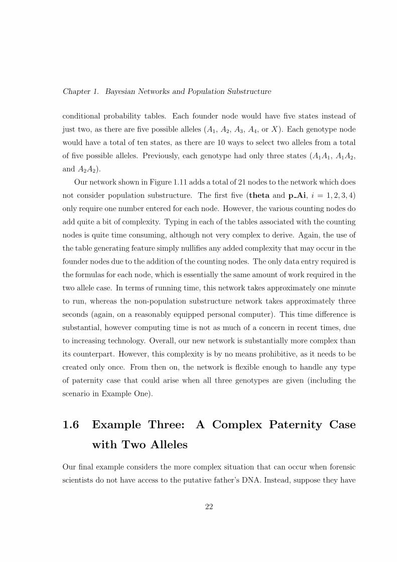
shown in Figure 1.15. We do in fact arrive at the same result given in Equation 1.11 by
Figure 1.15: HUGIN’s Output After Entering the Evidence, Complex Paternity Network.
dividing the percentages displayed in the table for tf=pf?, as is shown in Equation 1.12,
AI =66.18
33.82= 1.96. (1.12)
Here, we added a total of eight nodes (theta, Specified p, and the six counting
nodes). The resultant network has similar advantages and disadvantages to the network
created in Example One. It is a much more flexible network, and is actually simpler
to create than its non-population substructure counterpart (again, as a result of the
table generating feature).
25
This document is a research report submitted to the U.S. Department of Justice. This report has not been published by the Department. Opinions or points of view expressed are those of the author(s) and do not necessarily reflect the official position or policies of the U.S. Department of Justice.

Chapter 1. Bayesian Networks and Population Substructure
1.7 Discussion
Bayesian Networks are clearly a useful tool for DNA evidence evaluation. They allow
scientists to point and click their way to solutions for very difficult probability calcula-
tions. They also provide a graphical representation of, at times, highly complex forensic
scenarios. One way to fully make use of this valuable tool is to provide several “shell”
networks that can be used over and over again by anyone. This work contributes a few
“shells” that allow scientists to make inferences based on DNA evidence while taking
into account population substructure. With the advent of HUGIN, along with the
table generating feature, these networks are not only possible, but relatively simple to
create. Graphical methods, such as BNs, are bringing the power of complex statistical
methodology into the forensic laboratory. Here, we have presented an extension of an
already established graphical tool to further empower the forensic scientist.
26
This document is a research report submitted to the U.S. Department of Justice. This report has not been published by the Department. Opinions or points of view expressed are those of the author(s) and do not necessarily reflect the official position or policies of the U.S. Department of Justice.

Chapter 2
Pairwise Relatedness and Population
Substructure
2.1 Introduction
Pairwise relatedness describes the amount of relatedness between two individuals or
organisms. In our context, the amount of genetic similarity observed can be used as
a measure or indicator of relatedness. To illustrate, suppose two individuals are full
siblings. Their DNA will be made up of DNA passed down through their respective
ancestors. Since they are siblings, they have the exact same ancestors. As a result,
they will have a higher level of genetic similarity than an unrelated pair of individuals.
That is, the greater the number of ancestors in common (increasing relatedness) leads
to greater amounts of genetic similarity.
An important concept that helps describe genetic similarity is commonly referred
to as identity by descent or IBD. Two alleles are IBD if they are direct copies of a
single ancestral allele. For example, suppose X and Y are full siblings. Let X have
alleles labeled a and b, and let Y have alleles labeled c and d. This particular situation
is diagrammed in Figure 2.1. Here, there is a chance that a and c are IBD as they
could both be a copy of the same maternal allele.
An inbred individual is one that carries IBD alleles. Most populations will always
have a low level of inbreeding, due to population substructure. Inbreeding, of any
amount, will necessarily have an effect on pairwise relatedness estimates. If two indi-
viduals share some background relatedness due to inbreeding we would arrive at inflated
estimates of relatedness. It would be useful to quantify the effects of background relat-
27
This document is a research report submitted to the U.S. Department of Justice. This report has not been published by the Department. Opinions or points of view expressed are those of the author(s) and do not necessarily reflect the official position or policies of the U.S. Department of Justice.

Chapter 2. Pairwise Relatedness and Population Substructure
Mother Father
X Yab cd
?
a�
��c@
@@Rb
?
d
Figure 2.1: Diagram of IBD Relationship Between Two Siblings X and Y .
edness and incorporate them into our estimation technique. However, most pairwise
relatedness estimators developed thus far have ignored population substructure.
Accurately estimating pairwise relatedness is important in many diverse fields, in-
cluding forensic genetics, quantitative genetics, conservation genetics, and evolutionary
biology [23]. Perhaps the most common forensic application of pairwise relatedness
is in remains identification. Traditionally, dental records or fingerprints are used to
identify remains. However, in many cases these methods are impractical (high temper-
ature fires, explosive impact, etc.). Pairwise relatedness estimation can facilitate the
identification process in these cases. Indeed, within the last decade, several remains
identification projects have made extensive use of pairwise relatedness (kinship) esti-
mation [24, 25, 26, 27, 28]. In addition, there are scenarios where pairwise relatedness
estimates may be helpful in the courtroom. For example, the defense may suggest that
a relative of the suspect is the true culprit. An estimate of the amount of relatedness
between the suspect and the donor of the crime stain may be useful in this case. When
authorities are unable to apprehend a suspect and a crime stain is available, related-
ness estimation could be invaluable. If a known relative’s DNA is available, pairwise
relatedness estimation may give the authorities evidence to infer innocence or guilt.
28
This document is a research report submitted to the U.S. Department of Justice. This report has not been published by the Department. Opinions or points of view expressed are those of the author(s) and do not necessarily reflect the official position or policies of the U.S. Department of Justice.

Chapter 2. Pairwise Relatedness and Population Substructure
Measuring Pairwise Relatedness
One common measure of pairwise relatedness is referred to as the coancestry coefficient,
denoted θXY . It is defined as the probability a random allele from individual X is IBD
to a random allele from individual Y . To illustrate, consider the case where X and
Y are parent and child, respectively. Also assume there is no underlying population
substructure (non-inbred). Suppose X has alleles a and b. Due to Mendelian inher-
itance laws, with equal probability X will pass Y either allele a or allele b. Without
loss of generality, we assume that a is passed from X to Y . In this case, the prob-
ability of randomly selecting allele a from X is 1/2. In addition, the probability of
randomly selecting allele a from Y is also 1/2. This leads to an overall probability of
(1/2)(1/2) = 1/4, which is θXY in the parent-child case. Similar arguments can be
used to arrive at the other θXY values listed in Table 2.1. The relatedness coefficient
is another common measure, and is simply 2θXY (in the non-inbred case).
Table 2.1: Common θXY Values.
Relationship θXYUnrelated 0
Cousins 1/16
Full Siblings, Parent/Child 1/4
Identical Twins 1/2
The final and most descriptive method of measuring non-inbred pairwise relatedness
was first introduced by Cotterman [29]. It involves the use of three parameters, whose
definition here follows the notation of Evett and Weir [2]. Define P0, P1, and P2 as
the probability, at a particular locus, that two individuals share 0, 1, or 2 alleles IBD,
respectively. Figure 2.2 is a diagram of the possible IBD relationships (or patterns)
that could occur between four alleles taken from two individuals, X and Y . Later we
see when population substructure exists, there are nine possible IBD patterns. For
now we assume two alleles within the same individual cannot be IBD, thus only three
29
This document is a research report submitted to the U.S. Department of Justice. This report has not been published by the Department. Opinions or points of view expressed are those of the author(s) and do not necessarily reflect the official position or policies of the U.S. Department of Justice.

Chapter 2. Pairwise Relatedness and Population Substructure
s
s
s
s
S0
s
s
s
s
S1
s
s
s
s
S2
Figure 2.2: IBD Patterns Between Two Individuals, for the Non-Inbred Case.
In each group, the two upper dots represent the alleles in individual X. The two lower dots
represent the alleles in Y . A line between two dots indicates those alleles are IBD.
patterns are required. Consider the first diagram in Figure 2.2. There are two alleles
shared between X and Y that are IBD. Thus, the probability of this pattern occurring
is P2. The probability of the second pattern is then P1, and P0 is the probability of
the final pattern.
The coancestry coefficient can be written as a function of these “P -coefficients”.
Recall θXY is the probability a random allele from individual X is IBD to a random
allele from individual Y . In the first pattern, with probability 1/2 any random allele
from X will be IBD to a random allele from Y (half the time the IBD allele from Y
will be selected and half the time the non-IBD allele from Y will be selected). In the
second pattern, only half of the time will you select the IBD allele from X. When this
is coupled with the chance of selecting the IBD allele from Y (1/2), you arrive at an
overall probability of 1/4. The remaining pattern has no lines connecting X’s alleles
to Y ’s alleles and therefore does not contribute to the value of θXY . Thus the following
holds:
θXY =1
4P1 +
1
2P2. (2.1)
The coancestry coefficient, relatedness coefficient and P -coefficients are just a few
of the existing parameters which can be used to measure pairwise relatedness. The
purpose of this research is to adapt an existing estimator of pairwise relatedness. A
reliable and simple estimator of pairwise relatedness is sought that can account for the
30
This document is a research report submitted to the U.S. Department of Justice. This report has not been published by the Department. Opinions or points of view expressed are those of the author(s) and do not necessarily reflect the official position or policies of the U.S. Department of Justice.

Chapter 2. Pairwise Relatedness and Population Substructure
potential effects of population substructure.
2.2 Review of Relevant Literature
Pairwise relatedness estimation is important in several diverse fields of study. As a
result, several estimators of pairwise relatedness have been proposed using a variety of
methodologies. The most commonly used technique (Queller and Goodnight [30]) was
derived from a quantitative genetics point of view. The second group of estimators we
consider makes use of the method of moments. Finally, maximum likelihood estimators
will be reviewed. Note that the maximum likelihood approach will receive the most
attention, as it is the foundation for the new estimator proposed. A comprehensive
review of all techniques listed above is found in [23] and a biologist’s perspective is
given in [31]. A statistical comparison of several estimators (oddly excluding maximum
likelihood) is found in [32].
In 2003, Milligan performed a simulation study designed to compare various pair-
wise relatedness estimators [33]. Several currently used estimators, including those
we consider here, were examined. The results obtained are in agreement with most
other studies. As a general rule, the amount of available genetic information impacts
the quality of any pairwise relatedness estimator(i.e. number of loci, number of alle-
les, allele frequency distributions). Thus, Milligan used several simulated data sets.
The number of loci ranged from five to thirty, and the number of alleles ranged from
two to twenty. Allele frequencies were taken from three types of distributions: equal
frequencies, one highly frequent allele (0.8), Dirichlet distribution with all parameters
one. The findings of this study will be referred to often when comparing the various
methods we consider in this section.
31
This document is a research report submitted to the U.S. Department of Justice. This report has not been published by the Department. Opinions or points of view expressed are those of the author(s) and do not necessarily reflect the official position or policies of the U.S. Department of Justice.

Chapter 2. Pairwise Relatedness and Population Substructure
Queller and Goodnight’s Estimator
A commonly used technique for estimating pairwise relatedness was studied by Queller
and Goodnight [30], though it was first derived by Grafen [34]. The estimate is of the
relatedness coefficient (rXY ) as opposed to the coancestry coefficient (θXY ). They de-
rive an estimator for the average relatedness between groups of individuals, as opposed
to pairs. However, they provide a modification of this method for pairwise estimation.
The derivation provided in both [30, 34] is based on quantitative genetic theory. The
reader is referred to [30] for details, as they are outside the scope of this review. Here,
we will simply describe the estimator and discuss the advantages and disadvantages of
using this technique.
First, define alleles to be identical in state (IBS) if they are of the same allelic type.
It is important to note the difference between IBS and IBD. Alleles which are IBD are
required to be IBS as well, because they are copies of the exact same ancestral allele.
However, the reverse is not true. If two alleles are IBS, they could have descended from
two different individuals (therefore not IBD). Next, label individual X’s alleles as a
and b, and individual Y ’s alleles as c and d (these are just labels and do not necessarily
imply different allelic types). Now we define indicator variables,
Sij =
1 if allele i is IBS to allele j,
0 otherwise.(2.2)
Finally, let pi represent the population frequency of the ith allele. Queller and Good-
night’s estimate of rXY is then
rxy =0.5(Sac + Sad + Sbc + Sbd) − pa − pb
1 + Sab − pa − pb. (2.3)
The value of rxy will depend on which individual is assigned the label X and which is
Y . To arrive at an overall estimate, they propose using the average:
rXY + rY X2
. (2.4)
32
This document is a research report submitted to the U.S. Department of Justice. This report has not been published by the Department. Opinions or points of view expressed are those of the author(s) and do not necessarily reflect the official position or policies of the U.S. Department of Justice.

Chapter 2. Pairwise Relatedness and Population Substructure
Queller and Goodnight’s estimator is undefined when individual X is a heterozygote
and there are only two alleles. In addition, it is possible to arrive at estimates that are
outside the meaningful parameter space (0, 12). According to Milligan’s [33] simulations,
this estimator is unbiased, although it tends to have a left skewed distribution. Thus,
the most probable estimate will often be an incorrect one. The standard error for this
estimate, as with all others considered, decreases with increasing numbers of loci and
alleles. A major advantage of this method is that the creators have posted a program
online that is free to download and simple to use 1.
Moment Estimators
Several moment estimators have been developed to estimate pairwise relatedness [35,
36, 37, 23, 1, 38]. Two techniques are reviewed here: Li et al.’s [36] modification of
Lynch’s [35] estimator; Lynch and Ritland’s [23] estimator. Of the other moment esti-
mators, some are algebraically complex and others are very similar to those described
below and are thus not considered in this review. Appendix B contains comments and
corrections to the paper by Jinliang Wang [1].
Lynch and Li Estimator
First we consider Lynch’s [35] moment estimator, incorporating a slight modification
by Li et al. [36]. They are also estimating the relatedness coefficient. To begin, define
the similarity index (SXY ) as the average fraction of alleles at a locus in either X or
Y for which there is another allele in the other individual which is IBS. For example,
suppose X has genotype AiAi and Y has genotype AiAj . Both of X’s alleles are IBD
to an allele from Y . Additionally, one of Y ’s two alleles are IBD to an allele from X.
Thus SXY equals the average of 22
and 12
which is 34. Table 2.2 lists the SXY values
for all nine possible IBS patterns, denoted λ1, . . . , λ9. The concept behind Lynch’s
estimator is if two individuals are related to a degree rXY , the expected value of SXY is
1http://www.gsoftnet.us/GSoft.html
33
This document is a research report submitted to the U.S. Department of Justice. This report has not been published by the Department. Opinions or points of view expressed are those of the author(s) and do not necessarily reflect the official position or policies of the U.S. Department of Justice.

Chapter 2. Pairwise Relatedness and Population Substructure
Table 2.2: Similarity Index (SXY ) Values for All IBS Patterns.
IBS Patterns SXY
λ1 AiAi, AiAi ∀i 1
λ2 AiAi, AjAj ∀i,∀j 6= i 0
λ3 AiAi, AiAj ∀i,∀j 6= i 3/4
λ4 AiAi, AjAk ∀i,∀j 6= i,∀k > j, k 6= i 0
λ5 AiAj , AiAi ∀i,∀j 6= i 3/4
λ6 AjAk, AiAi ∀i,∀j 6= i,∀k > j, k 6= i 0
λ7 AiAj , AiAj ∀i,∀j > i 1
λ8 AiAj , AiAk ∀i,∀j 6= i,∀k 6= i, j 1/2
λ9 AiAj , AkAl ∀i,∀j > i,∀k 6= i, j,∀l > k, l 6= i, j 0
simply the sum of two terms. The first quantity is the fraction of alleles shared because
they are identical by descent and the second is the fraction shared because they are
identical in state. This leads to the following equation:
E(SXY ) = rXY + (1 − rXY )S0, (2.5)
where S0 is the expected value of SXY at a locus for two unrelated individuals in
a randomly mating population. The value of S0 is rarely known, and Li et al. [36]
propose S0 =∑n
i=1 p2i (2 − pi), where n is the number of alleles at the locus and pi is
the population frequency of the ith allele. Setting SXY equal to its expectation and
substituting in estimates for the unknown values, we have
SXY = rXY + (1 − rXY )S0. (2.6)
The moment estimator is then found by solving Equation 2.6 for rXY ,
rXY =SXY − S0
1 − S0
. (2.7)
To obtain a multi-locus estimate, the rXY values are simply averaged over loci.
Wang criticizes this approach, stating “although relatedness estimates from unlinked
34
This document is a research report submitted to the U.S. Department of Justice. This report has not been published by the Department. Opinions or points of view expressed are those of the author(s) and do not necessarily reflect the official position or policies of the U.S. Department of Justice.

Chapter 2. Pairwise Relatedness and Population Substructure
loci . . . are independent, they could be dramatically different in sampling variance and
ideally should not be simply averaged to give the overall estimate” [1]. Meaningful
values for rXY range from 0 to 1. It is important to note that Equation 2.7 does
require the estimates to be less than one, as SXY must be less than or equal to one.
It is possible to obtain a negative estimate, which would fall outside of the parameter
space. This happens whenever SXY < S0, which occurs at times due to sampling
error [23]. Also note this estimator is always defined, as long as at least one allele
frequency is greater than zero.
Lynch and Ritland’s Estimator
The next moment estimator was proposed by Lynch and Ritland [23]. To begin, define
two new parameters: φXY is the probability of X and Y having one pair of IBD alleles;
∆XY is the probability of X and Y having two pairs of IBD alleles. In our notation,
these two parameters are equivalent to P1 and P2. Lynch and Ritland use these param-
eters because in quantitative genetics, they are both involved in measuring the genetic
covariance between individuals. In particular, the additive genetic covariance between
individuals is a function of rXY , whereas the dominance genetic covariance is a function
of ∆XY . The relatedness coefficient can then be written in terms of these parameters:
rXY =φXY
2+ ∆XY . (2.8)
Lynch and Ritland focus on the conditional probabilities of individual Y ’s genotype
given individual X’s genotype. Here we will consider when Y is homozygous and refer
the reader to [23] for the other possible cases. Let Pr(ii|ii) denote the probability of X
and Y having two pairs of alleles in common and let Pr(ii|ii) denote the probability of
them having only one pair in common. Lynch and Ritland give these probabilities as
Pr(ii|ii) = p2i + pi(1 − pi)φXY + (1 − p2
i )∆XY , (2.9)
Pr(ii|ii) = 2pi(1 − pi) + (1 − pi)(1 − 2pi)φXY − 2pi(1 − pi)∆XY . (2.10)
35
This document is a research report submitted to the U.S. Department of Justice. This report has not been published by the Department. Opinions or points of view expressed are those of the author(s) and do not necessarily reflect the official position or policies of the U.S. Department of Justice.

Chapter 2. Pairwise Relatedness and Population Substructure
It is assumed that the population allele frequencies are known. To use the method of
moments, two functions are required whose expected values are Pr(ii|ii) and Pr(ii|ii).
Lynch and Ritland propose two indicator variables, that are assigned 1 if the corre-
sponding genotype pattern is observed and 0 is assigned for all other patterns. These
equations, with the indicator functions substituted in, can then be solved to obtain
estimates for φXY and ∆XY . Using Equation 2.8, and substituting in φXY and ∆XY
will give the estimator:
rXY =Pr(ii|ii) + 2Pr(ii|ii) − 2pi
2(1 − pi). (2.11)
As mentioned, the equation above holds only when Y is a homozygote. Lynch and
Ritland additionally provide a general form of their estimator that holds for all cases
(Equation 5 in [23]). Since their estimates will differ depending on which person is
labeled Y , they suggest averaging the two cases, as done by Queller and Goodnight
in Equation 2.4. Finally, to obtain multi-locus estimates they propose using a weight-
ing system. The actual weights that will minimize the variance of their estimator are
functions of parameters and thus cannot be obtained. Lynch and Ritland use approx-
imations which make the inconsistant assumption that X and Y are unrelated.
A major limitation of this estimation technique is this necessity to assume X and
Y are unrelated. It requires assuming a particular value for relatedness (namely 0),
when it is relatedness itself that we are trying to estimate. As with Queller and
Goodnight’s estimator above, this estimate can also be undefined. This occurs when
X is a heterozygote for a locus with two equally frequent alleles.
Another potential disadvantage is that negative estimates of rXY can occur. Ob-
taining estimates outside of the meaningful parameter space is an issue that deserves
some attention. Mainly due to the competing perspectives that exist about its mean-
ing. Lynch and Ritland state that these estimates are in fact meaningless, and it is a
drawback to using their estimators. Milligan and Wang agree [33, 1]. However, Hardy
states
It is important to keep in mind that relatedness coefficients depend on a
36
This document is a research report submitted to the U.S. Department of Justice. This report has not been published by the Department. Opinions or points of view expressed are those of the author(s) and do not necessarily reflect the official position or policies of the U.S. Department of Justice.
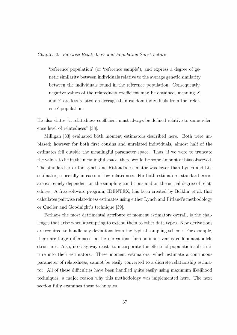
Chapter 2. Pairwise Relatedness and Population Substructure
‘reference population’ (or ‘reference sample’), and express a degree of ge-
netic similarity between individuals relative to the average genetic similarity
between the individuals found in the reference population. Consequently,
negative values of the relatedness coefficient may be obtained, meaning X
and Y are less related on average than random individuals from the ‘refer-
ence’ population.
He also states “a relatedness coefficient must always be defined relative to some refer-
ence level of relatedness” [38].
Milligan [33] evaluated both moment estimators described here. Both were un-
biased; however for both first cousins and unrelated individuals, almost half of the
estimates fell outside the meaningful parameter space. Thus, if we were to truncate
the values to lie in the meaningful space, there would be some amount of bias observed.
The standard error for Lynch and Ritland’s estimator was lower than Lynch and Li’s
estimator, especially in cases of low relatedness. For both estimators, standard errors
are extremely dependent on the sampling conditions and on the actual degree of relat-
edness. A free software program, IDENTEX, has been created by Belkhir et al. that
calculates pairwise relatedness estimates using either Lynch and Ritland’s methodology
or Queller and Goodnight’s technique [39].
Perhaps the most detrimental attribute of moment estimators overall, is the chal-
lenges that arise when attempting to extend them to other data types. New derivations
are required to handle any deviations from the typical sampling scheme. For example,
there are large differences in the derivations for dominant versus codominant allele
structures. Also, no easy way exists to incorporate the effects of population substruc-
ture into their estimators. These moment estimators, which estimate a continuous
parameter of relatedness, cannot be easily converted to a discrete relationship estima-
tor. All of these difficulties have been handled quite easily using maximum likelihood
techniques; a major reason why this methodology was implemented here. The next
section fully examines these techniques.
37
This document is a research report submitted to the U.S. Department of Justice. This report has not been published by the Department. Opinions or points of view expressed are those of the author(s) and do not necessarily reflect the official position or policies of the U.S. Department of Justice.

Chapter 2. Pairwise Relatedness and Population Substructure
Maximum Likelihood Estimators
As mentioned above, maximum likelihood techniques have been derived and adapted
to handle a wide variety of cases. They have been used to arrive at both a discrete
estimate (as done by Thompson [40]) and a continuous estimate of relatedness (as
in [33]). The likelihood technique has also been extended to incorporate the effects
of linkage between loci [41]. Hypothesis testing using the likelihood function has also
been explored [42]. A comprehensive review of earlier work in maximum likelihood
estimation and the handling of various extensions is provided in [43]. First we describe
the original maximum likelihood estimator (MLE) proposed in 1975 by Thompson [40].
Then we discuss how Milligan proposed expanding Thomson’s model from three to nine
parameters in order to allow for population substructure.
Three Parameter MLE
Likelihood techniques estimate the coancestry coefficient (θXY ) defined in Section 2.1.
The invariance property states if θ is the maximum likelihood estimator of θ, then for
any function τ(θ), the MLE of τ(θ) is τ(θ). This property implies that once we obtain
the MLEs for the three P -coefficients (defined in Section 2.1), we can use Equation 2.1
to find the MLE for θXY .
Assume we observe data on the genotypes of two individuals at several unlinked
loci. Nine distinct IBS patterns, λi, i = 1, . . . 9, were discussed in the previous section
(Table 2.2). The likelihood of P given an observed IBS pattern λi is
Li(P|λi) = Pr(λi|P). (2.12)
The subscript i on the likelihood makes it explicit that the likelihood function varies
based on which IBD pattern is observed. Let the three IBD patterns in Figure 2.2 be
S7, S8, and S9 (the purpose for this notation will become clear when we discuss the
nine parameter MLE). Then, making use of law of total probability (see Appendix A),
38
This document is a research report submitted to the U.S. Department of Justice. This report has not been published by the Department. Opinions or points of view expressed are those of the author(s) and do not necessarily reflect the official position or policies of the U.S. Department of Justice.

Chapter 2. Pairwise Relatedness and Population Substructure
we have
Li(P|λi) = Pr(λi|S7) Pr(S7) + Pr(λi|S8) Pr(S8) + Pr(λi|S9) Pr(S9)
= Pr(λi|S7)P2 + Pr(λi|S8)P1 + Pr(λi|S9)P0.(2.13)
If we denote the frequency of the ith allele as pi, the values for Pr(λi|Sj) are given in
Table 2.3. To illustrate, consider the first cell of Table 2.3. In this case, all alleles
Table 2.3: Conditional Probabilities Pr(λi|Sj), with No Population Substructure.
IBD Pattern
IBS Pattern S7 S8 S9
λ1 AiAi, AiAi p2i p3
i p4i
λ2 AiAi, AjAj 0 0 p2i p
2j
λ3 AiAi, AiAj 0 p2i pj 2p3
i pj
λ4 AiAi, AjAk 0 0 2p2i pjpk
λ5 AiAj , AiAi 0 p2i pj 2p3
i pj
λ6 AjAk, AiAi 0 0 2p2i pjpk
λ7 AiAj , AiAj 2pipj pipj(pi + pj) 4p2i p
2j
λ8 AiAj , AiAk 0 pipjpk 4p2i pjpk
λ9 AiAj , AkAl 0 0 4pipjpkpl
are of type i and we are given that two pairs of alleles are IBD. Thus, the probability
of this event is the chance that X randomly gets two i alleles. When there is no
population substructure, X receives the i alleles independently. Therefore it is simply
the frequency of the ith allele squared. The other cells can be determined using similar
arguments. This likelihood equation will be further examined and an example of its
use is provided in Section 2.3.
To obtain the MLEs for the P -coefficients we need to maximize the likelihood
with respect to the parameters of interest. In some cases, this can be performed
analytically (see Appendix A of [33]). However, in the majority of cases the maximum
must be found using some numerical maximizing technique. Here we use the downhill
simplex method which will be discussed at length in Section 2.3. To obtain multi-locus
39
This document is a research report submitted to the U.S. Department of Justice. This report has not been published by the Department. Opinions or points of view expressed are those of the author(s) and do not necessarily reflect the official position or policies of the U.S. Department of Justice.

Chapter 2. Pairwise Relatedness and Population Substructure
estimates, the likelihoods for each loci are simply multiplied together to arrive at one
overall likelihood function, as loci are assumed independent. This overall likelihood
is then maximized to obtain the MLE. Recalling the weighting method of Lynch and
Ritland that required the (perhaps incorrect) assumption thatX and Y were unrelated,
this multiplicative property of likelihoods is quite an advantage.
A disadvantage of the three dimensional maximum likelihood estimator is the large
biases that occur for some relationships. This problem can be severe if the relationship
is close to the endpoints of the parameter space. This bias occurs because the maximum
likelihood technique requires its estimates to fall within the valid space. For example,
if the true relationship is unrelated (θXY = 0), we will never get an unbiased result as
we are unable to obtain values less than zero. Milligan found that genetic sampling
has a large effect on the amount of bias, stating that it can be reduced by sampling
loci with more alleles (>20), with non-skewed frequency distributions [33]. Another
disadvantage is that software is not freely available to implement this method.
An advantage of the three parameter likelihood technique is the small standard
errors observed. Milligan showed, depending on sampling conditions, that the standard
errors for the non-likelihood based estimators were between 2% and 250% larger. In
addition he found that the errors for the MLE were less influenced by degree of actual
relatedness. This was not the case for the other estimators considered. When the root
mean-squared error was studied, the likelihood maintains very low values. To conclude,
Milligan writes “although some non-likelihood estimators exhibit better performance
with respect to specific metrics under some conditions, none approach the high level of
performance exhibited by the likelihood estimator across all conditions and all metrics
of performance.”
Overall, it seems clear that a maximum likelihood approach has many advantages
over the other estimators reviewed here. According to current studies, the bias that
is observed can be overcome by sampling a large number of loci, as well as increasing
the number of alleles. In previous decades, this has meant that the likelihood method
has fallen by the wayside. However, as technology is improving, vast amounts of
40
This document is a research report submitted to the U.S. Department of Justice. This report has not been published by the Department. Opinions or points of view expressed are those of the author(s) and do not necessarily reflect the official position or policies of the U.S. Department of Justice.

Chapter 2. Pairwise Relatedness and Population Substructure
genetic data are becoming available on a much larger number of species. Thus, the
likelihood method is gradually becoming a more popular method of pairwise relatedness
estimation.
Nine Parameter MLE
In 2003, Milligan extended the work of Thompson by defining the maximum likelihood
estimator in a way that can account for population substructure [33]. This natural
extension increases the number of parameters needed from three to nine. The previous
approach allowed for only three IBD patterns, as presented in Figure 2.2. When
population substructure exists, there are more possibilities. There is now a chance
that X’s (or Y ’s) parents have ancestors in common. This implies that the two alleles
received by an individual from their parent could be IBD. In particular, six additional
IBD patterns must be considered. The full set of nine IBD states Sj are shown in
Figure 2.3. This expanded set of patterns requires that nine parameters be estimated:
∆j = Pr(Sj) for j = 1, . . . , 9. (2.14)
They are referred to as Jacquard’s coefficients, as they were first developed by Jacquard
in [44]. The data we observe are the possible IBS patterns, λi, given in Table 2.3. Thus,
the nine parameter likelihood function is
Li(∆|λi) =9
∑
j=1
Pr(λi|Sj)∆j , (2.15)
as ∆j = Pr(Sj), and where Pr(λi|Sj) values are given in Table 2.4, adapted from [33].
We derive two cells here and refer the reader to [33] for further details.
Consider the cell in Table 2.4 corresponding to IBD pattern S4 (see Figure 2.3)
and IBS pattern λ3 (AiAi, AiAj). In this case, the two alleles from X are IBD to each
other, but no other alleles are IBD. Thus, we only need to include the probability of
obtaining allele Ai once (pi). The probability of Y having alleles AiAj , given there are
no IBD relationships involving these alleles is 2pipj. The factor of 2 is because order is
41
This document is a research report submitted to the U.S. Department of Justice. This report has not been published by the Department. Opinions or points of view expressed are those of the author(s) and do not necessarily reflect the official position or policies of the U.S. Department of Justice.

Chapter 2. Pairwise Relatedness and Population Substructure
s
s
s
s
���@
@@
S1
s
s
s
s
S2
s
s
s
s
���
S3
s
s
s
s
S4
s
s
s
s
@@@
S5
s
s
s
s
S6
s
s
s
s
S7
s
s
s
s
S8
s
s
s
s
S9
Figure 2.3: IBD Patterns Between Two Individuals, for the Inbred Case.
In each group, the two upper dots represent the alleles from individual X. The two lower
dots represent the alleles from Y . A line between two dots indicates those alleles are IBD.
Table 2.4: Conditional Probabilities Pr(λi|Sj), with Population Substructure.
S1 S2 S3 S4 S5 S6 S7 S8 S9
λ1 pi p2i p2
i p3i p2
i p3i p2
i p3i p4
i
λ2 0 pipj 0 pip2j 0 p2
i pj 0 0 p2i p
2j
λ3 0 0 pipj 2p2i pj 0 0 0 p2
i pj 2p3i pj
λ4 0 0 0 2pipjpk 0 0 0 0 2p2i pjpk
λ5 0 0 0 0 pipj 2p2i pj 0 p2
i pj 2p3i pj
λ6 0 0 0 0 0 2pipjpk 0 0 2p2i pjpk
λ7 0 0 0 0 0 0 2pipj pipj(pi + pj) 4p2i p
2j
λ8 0 0 0 0 0 0 0 pipjpk 4p2i pjpk
λ9 0 0 0 0 0 0 0 0 4pipjpkpl
42
This document is a research report submitted to the U.S. Department of Justice. This report has not been published by the Department. Opinions or points of view expressed are those of the author(s) and do not necessarily reflect the official position or policies of the U.S. Department of Justice.

Chapter 2. Pairwise Relatedness and Population Substructure
not considered within an individual; Y ’s alleles could be AiAj or AjAi. Therefore, the
probability of observing IBS pattern λ3 given IBD pattern S4 is 2p2i pj. Now consider
Pr(λ7|S8). Here we observe IBS pattern AiAj , AiAj and one allele from X is IBD to
one allele from Y . One possibility is that the Ai alleles are IBD. In this case, the
probability of observing the pattern is pip2j . If, instead, the Aj alleles are IBD the
probability of observing λ7 is p2i pj. When these two probabilities are summed, we
arrive at pipj(pi + pj).
Thus, Milligan has defined a likelihood that can be maximized to find the MLEs
of Jacquard’s coefficients. Making use of the MLE’s invariance property, an MLE for
θXY can be obtained. Recall θXY is the probability a random allele from individual
X is IBD to a random allele from individual Y . Using this definition, we can relate
Jacquard’s parameters to θXY :
θXY = ∆1 +1
2(∆3 + ∆5 + ∆7) +
1
4∆8. (2.16)
To arrive at this equation, consider the state S1 in Figure 2.3. In this case, with
probability one, any random allele from X will be IBD to a random allele from Y . In
state S3, with probability 1/2 any random allele from X will be IBD to a random allele
from Y (half the time the IBD allele from Y will be selected and half the time the
non-IBD allele from Y will be selected). The same is true for patterns S5 and S7. In S8
only half of the time will you select the IBD allele from X. When this is coupled with
the chance of selecting the IBD allele from Y (1/2), you arrive at an overall probability
of 1/4. The remaining states (S2, S4, S6, and S9) have no lines connecting X’s alleles
to Y ’s alleles and therefore do not contribute to the value of θXY .
After providing this derivation, Milligan finishes his study performing simulations
comparing the various aforementioned estimators. He simply ignores the effects of
population substructure, and performs his studies using the simplified three parameter
model presented above. No detailed study of the properties of the nine parameter
estimator has been done. For this reason, the nine parameter estimator is further
examined in the next section.
43
This document is a research report submitted to the U.S. Department of Justice. This report has not been published by the Department. Opinions or points of view expressed are those of the author(s) and do not necessarily reflect the official position or policies of the U.S. Department of Justice.

Chapter 2. Pairwise Relatedness and Population Substructure
2.3 Research Methods
This section extends the body of work on the estimation of relatedness using maximum
likelihood techniques. First, an example of the use of the nine parameter MLE is
provided. Similar to the three parameter MLE, analytical expressions for the MLE do
not exist and numerical methods must be employed. The downhill simplex method
is reviewed an examples of its use are provided. A new seven parameter estimator is
also derived that still accounts for population substructure while reducing the number
of parameters to estimate. Finally, a new methodology is developed that can infer
relationships from any of the three types of MLE estimates. We conclude by describing
the design of the simulation study used to compare the three, seven and nine paramter
MLEs.
Nine Parameter MLE, Continued
To facilitate the understanding of the nine parameter likelihood function given by
Equation 2.15, consider the following scenario. Suppose we observe genotype data for
two individuals at two loci. Let individual X have alleles A1A2 at locus one and B1B2
at locus two. Let individual Y have alleles A1A1 at locus one and B1B2 at locus two.
Label the allele frequencies p1, p2 and q1, q2 at the two loci, respectively. Consider the
first locus, with IBS pattern λ5 (AiAj , AiAi). Using Equation 2.15, coupled with the
appropriate line from Table 2.4 we find the likelihood for locus one is
L5(∆|λ5) =
9∑
j=1
Pr(λ5|Sj)∆j = p1p2∆5 + 2p21p2∆6 + p2
1p2∆8 + 2p31p2∆9. (2.17)
Now consider the second locus, and assume it is independent (unlinked) from the
first locus. Here, the IBS pattern is λ7 (BiBj, BiBj). The corresponding line from
Table 2.4 leads to the likelihood
L7(∆|λ7) =
9∑
j=1
Pr(λ7|Sj)∆j = 2q21q2∆7 + q1q2(q1 + q2)∆8 + 4q2
1q22∆9. (2.18)
44
This document is a research report submitted to the U.S. Department of Justice. This report has not been published by the Department. Opinions or points of view expressed are those of the author(s) and do not necessarily reflect the official position or policies of the U.S. Department of Justice.

Chapter 2. Pairwise Relatedness and Population Substructure
Since the loci are independent, we simply multiply the two likelihoods together to
obtain an overall likelihood,
L(∆) =(
p1p2∆5 + 2p21p2∆6 + p2
1p2∆8 + 2p31p2∆9
)
×(
2q21q2∆7 + q1q2(q1 + q2)∆8 + 4q2
1q22∆9
)
.(2.19)
Now we need to maximize the likelihood, using some numerical method. Additional
complexity is introduced as we have the following constraints on our parameters:
•∑9
i=1 ∆i = 1,
• 0 ≤ ∆i ≤ 1, ∀i.
The first constraint is due to the fact that the nine IBD states are exhaustive, thus
their total probability must equal one. The second constraint is simply a result of
each parameter representing a probability, thus must lie between zero and one. One
numerical technique that caters to functions with constraints is the downhill simplex
method. For a complete description of the method, see [45]. The next section briefly
describes the method and continues this example.
Downhill Simplex Method
The downhill simplex method was first described by Nelder and Mead [46]. This
method was chosen because it is fast and accurate. Additional random walk methods
were attempted, however the estimates obtained were exactly those of the simplex
method. Additionally, the random walk programs took several hours to run, whereas
the simplex method only needed seconds. The simplex method was also employed in
Milligan’s study [33], allowing for verification of results.
The downhill simplex method is a numerical minimizing technique that facilitates
functions with constraints. An N -dimensional simplex is a geometrical figure of N + 1
points and all connecting line segments and faces. (In 2-dimensions it is a triangle.)
To begin, an initial simplex must be given. The method will then take a series of steps
changing the dimensions of the simplex. Each step either reflects, expands, or contracts
the simplex allowing the simplex to “blob” around the surface of the function, always
45
This document is a research report submitted to the U.S. Department of Justice. This report has not been published by the Department. Opinions or points of view expressed are those of the author(s) and do not necessarily reflect the official position or policies of the U.S. Department of Justice.

Chapter 2. Pairwise Relatedness and Population Substructure
searching for lower values. Eventually the simplex will pull itself in around the lowest
point, which will be the minimum value. Throughout the process, there are constant
checks to ensure the constraints are met. A C++ program was created implementing
this method (see Appendix C), adapting code provided in [45]. As mentioned, this is
a minimizing routine. Here we obtain the maximum value by minimizing the negative
likelihood.
Recall the likelihood equation for the example provided in the previous section:
L(∆) =(
p1p2∆5 + 2p21p2∆6 + p2
1p2∆8 + 2p31p2∆9
)
×(
2q21q2∆7 + q1q2(q1 + q2)∆8 + 4q2
1q22∆9
)
.(2.20)
We would like to maximize the likelihood with respect to ∆. For demonstration pur-
poses, we consider the special case where no population substructure exists. This
assumption requires ∆1 = . . . = ∆6 = 0. If we additionally assume (arbitrarily) that
p1 = p2 = q1 = q2 = 0.30, and note that ∆9 = 1−∆7 −∆8, the likelihood is reduced to
L(∆) = −0.0215∆27 − 0.0037∆2
8 + 0.0168∆7 + 0.0063∆8 + 0.0047. (2.21)
Figure 2.4 provides a graph of this function.
To get a better idea of where the maximum occurs, Figure 2.5 shows the likelihood
with an intercepting plane, showing the maximum occurs when ∆7 ≈ 0.40 and ∆8 ≈ 0.
We can use the simplex method to obtain exact results. The following is output from
our program:
Delta 7 = 0.390
Delta 8 = 0.0
Delta 9 = 0.610
Maximum = 0.008
Theta_XY = 0.195
This method required 254 function evaluations
As predicted above, the MLEs for ∆7 and ∆8 are 0.390 and 0, respectively. The MLE
for ∆9 is simply one minus the MLE values for ∆7 and ∆8. The output gives us the
actual value of the likelihood at the maximum, 0.008, which also agrees with our plots
46
This document is a research report submitted to the U.S. Department of Justice. This report has not been published by the Department. Opinions or points of view expressed are those of the author(s) and do not necessarily reflect the official position or policies of the U.S. Department of Justice.

Chapter 2. Pairwise Relatedness and Population Substructure
∆∆∆∆7∆∆∆∆8
Likelih
oo
d
∆∆∆∆7∆∆∆∆8
Likelih
oo
d
Figure 2.4: Graph of Likelihood Function.
∆∆∆∆7
∆∆∆∆8
Likelih
oo
d
∆∆∆∆7
∆∆∆∆8
Likelih
oo
d
Figure 2.5: Graph of Likelihood Function with Intercepting Plane.
47
This document is a research report submitted to the U.S. Department of Justice. This report has not been published by the Department. Opinions or points of view expressed are those of the author(s) and do not necessarily reflect the official position or policies of the U.S. Department of Justice.

Chapter 2. Pairwise Relatedness and Population Substructure
in Figures 2.4 and 2.5. The MLE for θXY is given, which we can verify using using
Equation 2.16:
(θXY )MLE =1
2(0.390) +
1
4(0) = 0.195. (2.22)
Finally, the number of function evaluations required is also listed in the output. This
refers to how many times the likelihood function was computed for a particular set
of parameter values before the “best” value was obtained. The computationally de-
manding portion of this program is the function evaluations. Thus, the number of
evaluations is reported to give an idea of how long the program took to run. In this
case, it only took a fraction of a second. While this simplified example was in two
dimensions, the simplex method works exactly the same in N -dimensions (N = 8 in
the population substructure case).
The nine dimensional method requires a distinction between X and Y . In some
cases, this distinction is not necessary. For example, if X and Y are drawn from
the same subpopulation, the probability that X has two IBD alleles is equal to the
probability that Y has two IBD alleles. The nine parameter model assumes these two
probabilities are distinct. If the distinction between X and Y is unnecessary the nine
parameter model is at a disadvantage, as extraneous parameters are being estimated.
This is the motivation for the seven parameter model proposed in the next section.
Seven Parameter MLE
As mentioned, in the nine parameter case different estimates can occur depending on
which individual is labeled X and which is labeled Y . This phenomenon occurs because
the patterns shown in Figure 2.3 are ordered with respect to X and Y . For example,
if we were to ignore the ordering of X and Y , S3 and S5 would be the same pattern.
In addition, S4 and S6 would also be the same pattern. If we assume X and Y come
from the same subpopulations, one new parameter could replace ∆3 and ∆5. If another
parameter replaced ∆4 and ∆6, the total number of parameters is reduced to seven.
A new set of notation is needed to define the seven parameter estimate. To begin,
48
This document is a research report submitted to the U.S. Department of Justice. This report has not been published by the Department. Opinions or points of view expressed are those of the author(s) and do not necessarily reflect the official position or policies of the U.S. Department of Justice.

Chapter 2. Pairwise Relatedness and Population Substructure
there are now only seven distinct IBD patterns possible between the four alleles from
X and Y . These patterns are denoted S ′
1, . . . S′
7 and are shown in Figure 2.6. Pattern
s
s
s
s
���@@@
R1
s
s
s
s
R2
s
s
s
s
���
R3
s
s
s
s
R4
s
s
s
s
R5
s
s
s
s
R6
s
s
s
s
R7
Figure 2.6: IBD Patterns Between Two Individuals, for the Seven Parameter Inbred Case.
S ′
3 replaces both S3 and S5 from Figure 2.3, as the ordering between X and Y does not
matter. Similarly, S ′
4 replaces both S4 and S6. Thus, the new parameters of interest
are
φj = Pr(S ′
j) for j = 1, . . . , 7. (2.23)
A description of the relationships among the new φ’s, Jacquard’s coefficients, and Evett
and Weir’s commonly used δ coefficients [2] is given in Table 2.5.
In addition to reducing the number of IBD states, we also reduce the number of IBS
states. Now that ordering between X and Y no longer matters, pattern λ3 (AiAi, AiAj)
is the same as pattern λ5 (AiAj , AiAi). Similarly, λ4 (AiAi, AjAk) is the same as λ6
(AjAk, AiAi). Thus, we define a new set of IBS patterns, λ′1, . . . , λ′
7 and they are listed
in Table 2.6. The likelihood is similar to that in Equation 2.15,
Li(∆|λ′i) =
7∑
j=1
Pr(λ′i|S′
j)φj, (2.24)
where Pr(λ′i|S′
j) is given by Table 2.6.
49
This document is a research report submitted to the U.S. Department of Justice. This report has not been published by the Department. Opinions or points of view expressed are those of the author(s) and do not necessarily reflect the official position or policies of the U.S. Department of Justice.
Chapter 2. Pairwise Relatedness and Population Substructure
Table 2.5: Relationships Among Various Relateness Coefficients.
New Jacquard [44] Evett & Weir [2]
φ1 ∆1 δabcdφ2 ∆2 δab.cdφ3 ∆3 + ∆5 δabc + δabd + δacd + δbcdφ4 ∆4 + ∆6 δab + δcdφ5 ∆7 δac.bd + δad.bcφ6 ∆8 δac + δbd + δad + δbcφ7 ∆9 δ0
Table 2.6: Conditional Probabilities based on Seven Parameters.
IBSPatterns S ′
1 S ′
2 S ′
3 S ′
4 S ′
5 S ′
6 S ′
7
λ′1 = AiAi, AiAi pi p2i p2
i p3i p2
i p3i p4
i
λ′2 = AiAi, AjAj 0 pipj 0 pip2j 0 0 p2
i p2j
λ′3 = AiAi, AiAj 0 0pipj
2p2i pj 0 p2
i pj 2p3i pj
λ′4 = AiAi, AjAk 0 0 0 pipjpk 0 0 2p2i pjpk
λ′5 = AiAj , AiAj 0 0 0 0 2pipj pipj(pi + pj) 4p2i p
2j
λ′6 = AiAj , AiAk 0 0 0 0 0 pipjpk 4p2i pjpk
λ′7 = AiAj , AkAl 0 0 0 0 0 0 4pipjpkpl
To demonstrate the conversion from the nine by nine Table 2.4 to the seven by
seven table here, consider the first row. The value for Pr(S ′
3|λ′
1) is simply the average
of the appropriate probabilities from Table 2.4:
Pr(S ′
3|λ′
1) =Pr(S3|λ1) + Pr(S5|λ1)
2=p2i + p2
i
2= p2
i . (2.25)
Similarly,
Pr(S ′
4|λ′
1) =Pr(S4|λ1) + Pr(S6|λ1)
2=p3i + p3
i
2= p3
i . (2.26)
The other entries in the first row are the exact same as those in Table 2.4, noting
S7 = S ′
5, S8 = S ′
6, S9 = S ′
7. The same process is used to arrive at the values for rows
50
This document is a research report submitted to the U.S. Department of Justice. This report has not been published by the Department. Opinions or points of view expressed are those of the author(s) and do not necessarily reflect the official position or policies of the U.S. Department of Justice.

Chapter 2. Pairwise Relatedness and Population Substructure
2, 5, 6, and 7. Now consider the third row of Table 2.6. The first two and last three
cells are obtained by averaging the corresponding values from Table 2.4 in the third
and fifth rows. For example, Pr(λ′3|S′
6 is the average of p2i pj and p2
i pj . Pr(S ′
3|λ′
3) is
obtained by averaging four cells from Table 2.4,
Pr(S ′
3|λ′
3) =Pr(S3|λ3) + Pr(S5|λ3) + Pr(S3|λ5) + Pr(S5|λ5)
4. (2.27)
A similar average is used for the next cell,
Pr(S ′
4|λ′
3) =Pr(S4|λ3) + Pr(S6|λ3) + Pr(S4|λ5) + Pr(S6|λ5)
4. (2.28)
The fourth row is derived in a similar manner to row three.
Therefore, we have defined a likelihood that can be maximized to find the MLEs
for φ1, . . . φ7. The relationship between these parameters and the coancestry coeficient,
θXY = φ1 +1
2(φ3 + φ5) +
1
4φ6, (2.29)
allows us to obtain the MLE for θXY , similar to the nine parameter case.
Both the seven and nine parameter models give one summary value (MLE of θXY )
which can then be used to infer a relationship. For example, if we get an estimate
of 0.24 and if there is no inbreeding, and the ages of X and Y are fairly close (to
rule out the parent-child possibility), we could predict that it is a full sibling pair.
Unfortunately, this is not the most satisfying result. We would like to say they are full
siblings with absolute certainty, or with at least some idea of the error rates associated
with our estimate. In addition, we may not have information about the individuals’
ages. Thus, it would be impossible to differentiate between full sibling and parent-child
pairs. Ideally, we would like to have some sort of classification mechanism that could
place paired observations into one of several groups. Then an estimated relationship
could be given, as well as some accuracy rates based on simulation study results. To
this end, a distance metric method of classifying pairwise relationships was developed.
51
This document is a research report submitted to the U.S. Department of Justice. This report has not been published by the Department. Opinions or points of view expressed are those of the author(s) and do not necessarily reflect the official position or policies of the U.S. Department of Justice.

Chapter 2. Pairwise Relatedness and Population Substructure
Distance Metric Method of Relationship Classification
Through maximizing the likelihood, we have obtained estimates for either Jacquard’s
nine coefficients or the seven φ’s. When estimating the continuous parameter θXY , we
use only a function of these parameters. Additionally, that function only contains five
of the nine (or four of the seven) parameters estimated. In our classification method we
make use of all available MLE values; hypothesizing that the more information used,
the better the estimates.
To begin, we can quantify the amount of population substructure that exists using
what is commonly referred to as the inbreeding coefficient, denoted ψ. (Note that this
is the same parameter as θ defined in Chapter 1, it is relabeled here to avoid confusion
with θXY .) If we assume the value of ψ is known, it is possible to determine the true
values for either Jacquard’s coefficients or the seven φ’s for any imaginable relationship.
The true values of Jacquard’s coefficients, in terms of ψ, for some common relationships
are given in Table 2.7. Numerical values for the full sibling case, at several different
values of ψ, are given in Table 2.8.
Next, define ∆U , ∆F , . . . to be the known relationship vectors for unrelated pairs,
full sib pairs, etc. We can then compute the Euclidean distance (DU , DF , . . .) between
the estimated vector (∆) and several of the true vectors. For example, the distance
formula for unrelated individuals in the nine parameter case is
DU = ‖∆− ∆U‖ =
√
√
√
√
9∑
i=1
(∆i − ∆U,i)2, (2.30)
These distances can be computed for any number of competing relationships. The
relationship that obtains the minimum distance will then become our discrete estimate.
To illustrate the classification method, suppose we obtain the following nine parameter
MLE:
∆ = (0.0524, 0.0000, 0.0336, 0.0358, 0.0517, 0.0631, 0.0527, 0.4605, 0.2502). (2.31)
Assume we have prior knowledge that unrelated, cousin, half sib, and full sib pairs are
52
This document is a research report submitted to the U.S. Department of Justice. This report has not been published by the Department. Opinions or points of view expressed are those of the author(s) and do not necessarily reflect the official position or policies of the U.S. Department of Justice.
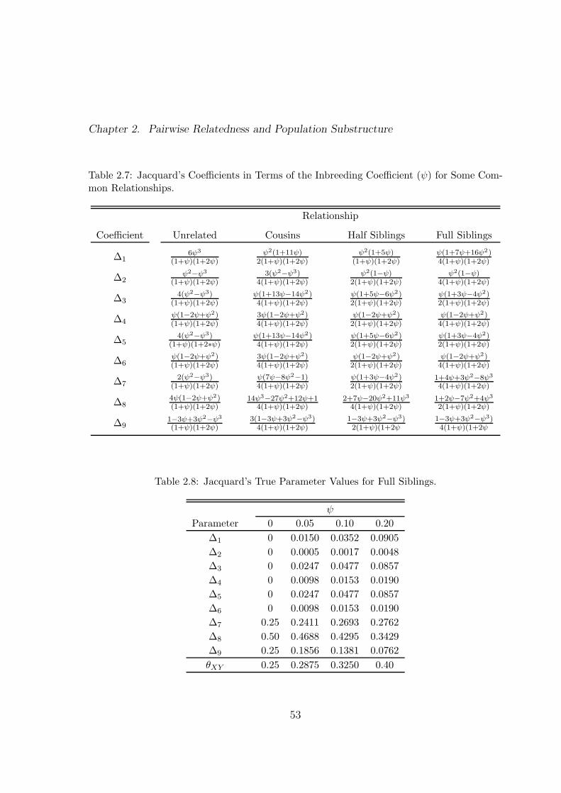
Chapter 2. Pairwise Relatedness and Population Substructure
Table 2.7: Jacquard’s Coefficients in Terms of the Inbreeding Coefficient (ψ) for Some Com-mon Relationships.
Relationship
Coefficient Unrelated Cousins Half Siblings Full Siblings
∆16ψ3
(1+ψ)(1+2ψ)ψ2(1+11ψ)
2(1+ψ)(1+2ψ)ψ2(1+5ψ)
(1+ψ)(1+2ψ)ψ(1+7ψ+16ψ2)4(1+ψ)(1+2ψ)
∆2ψ2
−ψ3
(1+ψ)(1+2ψ)3(ψ2
−ψ3)4(1+ψ)(1+2ψ)
ψ2(1−ψ)2(1+ψ)(1+2ψ)
ψ2(1−ψ)4(1+ψ)(1+2ψ)
∆34(ψ2
−ψ3)(1+ψ)(1+2ψ)
ψ(1+13ψ−14ψ2)4(1+ψ)(1+2ψ)
ψ(1+5ψ−6ψ2)2(1+ψ)(1+2ψ)
ψ(1+3ψ−4ψ2)2(1+ψ)(1+2ψ)
∆4ψ(1−2ψ+ψ2)(1+ψ)(1+2ψ)
3ψ(1−2ψ+ψ2)4(1+ψ)(1+2ψ)
ψ(1−2ψ+ψ2)2(1+ψ)(1+2ψ)
ψ(1−2ψ+ψ2)4(1+ψ)(1+2ψ)
∆54(ψ2
−ψ3)(1+ψ)(1+2∗ψ)
ψ(1+13ψ−14ψ2)4(1+ψ)(1+2ψ)
ψ(1+5ψ−6ψ2)2(1+ψ)(1+2ψ)
ψ(1+3ψ−4ψ2)2(1+ψ)(1+2ψ)
∆6ψ(1−2ψ+ψ2)(1+ψ)(1+2ψ)
3ψ(1−2ψ+ψ2)4(1+ψ)(1+2ψ)
ψ(1−2ψ+ψ2)2(1+ψ)(1+2ψ)
ψ(1−2ψ+ψ2)4(1+ψ)(1+2ψ)
∆72(ψ2
−ψ3)(1+ψ)(1+2ψ)
ψ(7ψ−8ψ2−1)
4(1+ψ)(1+2ψ)ψ(1+3ψ−4ψ2)2(1+ψ)(1+2ψ)
1+4ψ+3ψ2−8ψ3
4(1+ψ)(1+2ψ)
∆84ψ(1−2ψ+ψ2)(1+ψ)(1+2ψ)
14ψ3−27ψ2+12ψ+1
4(1+ψ)(1+2ψ)2+7ψ−20ψ2+11ψ3
4(1+ψ)(1+2ψ)1+2ψ−7ψ2+4ψ3
2(1+ψ)(1+2ψ)
∆91−3ψ+3ψ2
−ψ3
(1+ψ)(1+2ψ)3(1−3ψ+3ψ2
−ψ3)4(1+ψ)(1+2ψ)
1−3ψ+3ψ2−ψ3)
2(1+ψ)(1+2ψ1−3ψ+3ψ2
−ψ3)4(1+ψ)(1+2ψ
Table 2.8: Jacquard’s True Parameter Values for Full Siblings.
ψ
Parameter 0 0.05 0.10 0.20
∆1 0 0.0150 0.0352 0.0905
∆2 0 0.0005 0.0017 0.0048
∆3 0 0.0247 0.0477 0.0857
∆4 0 0.0098 0.0153 0.0190
∆5 0 0.0247 0.0477 0.0857
∆6 0 0.0098 0.0153 0.0190
∆7 0.25 0.2411 0.2693 0.2762
∆8 0.50 0.4688 0.4295 0.3429
∆9 0.25 0.1856 0.1381 0.0762
θXY 0.25 0.2875 0.3250 0.40
53
This document is a research report submitted to the U.S. Department of Justice. This report has not been published by the Department. Opinions or points of view expressed are those of the author(s) and do not necessarily reflect the official position or policies of the U.S. Department of Justice.

Chapter 2. Pairwise Relatedness and Population Substructure
the only possible relationships. Also suppose the population we are considering has
a (rather large) inbreeding coefficient of 0.10. Then for each possible relationship, we
can list the true vectors and compute DU , DC , DH , and DF which appear in Table 2.9.
From these results, we estimate the true relationship to be half siblings, as 0.0048 is
Table 2.9: MLE, True ∆ Vectors, and Euclidean Distances for Example in Section 2.3.
∆ ∆U ∆C ∆H ∆F
0.0524 0.0045 0.0080 0.0114 0.0352
0.0000 0.0068 0.0051 0.0034 0.0017
0.0336 0.0273 0.0409 0.0545 0.0477
0.0358 0.0614 0.0460 0.0307 0.0153
0.0517 0.0273 0.0409 0.0545 0.0477
0.0631 0.0614 0.0460 0.0307 0.0153
0.0527 0.0136 0.0307 0.0477 0.2693
0.4605 0.2455 0.3682 0.4909 0.4295
0.2502 0.5523 0.4142 0.2761 0.1381
Distances 0.1427 0.0385 0.0048 0.0637
the minimum distance observed. In fact, these data were simulated assuming half sib
relationship. The same methodology applies to the two or seven parameter model,
and comparisons among the these classification methods are included in the simulation
study described in the next section.
Experimental Design
A simulation study was designed to evaluate the performance of the seven and nine
parameter MLE, as well as the various distance metric methods of classification. We
wanted to determine the advantage (or disadvantage) of accounting for population
substructure in various population types. Thus, we simulated data assuming inbreeding
coefficients of 0, 0.05, 0.10. As Milligan notes, the quality of our estimates will depend
highly on the number of loci and the number of alleles per locus [33]. We considered
54
This document is a research report submitted to the U.S. Department of Justice. This report has not been published by the Department. Opinions or points of view expressed are those of the author(s) and do not necessarily reflect the official position or policies of the U.S. Department of Justice.
Chapter 2. Pairwise Relatedness and Population Substructure
2, 5, and 10 alleles for 20, 40, 60, 80 and 100 loci to evaluate these effects. When
ψ > 0, allele frequencies were assumed to come from a Dirichlet distribution, with
parameter (1 − ψ)pi/ψ. This particular Dirichlet distribution is appropriate in the
population substructure case [2]. Equal allele frequencies were assumed when ψ = 0.
Finally, we varied the true relationship to include unrelated, cousin, half sibling, and
full sibling pairs. For each combination of estimation method, allele number, loci
number, inbreeding coefficient and true relationship we simulated 500 observations. In
this study, the other pairwise relatedness estimators discussed in Section 2.2 were not
included, as previous comparison studies have been done [33, 23, 32].
2.4 Results
Continuous Estimation of θXY
We refer to the three parameter estimator as the 2D MLE as the maximization takes
place in two dimensional space. 6D MLE and 8D MLE refer to the seven and nine
parameter estimates, respectively. Several plots representing the mean values 2D MLE
are shown in Figure 2.7. Increasing the number of both loci and alleles increases the
accuracy of the estimator in the non-inbred case (ψ = 0.0). However, this trend does
not continue as ψ increases. In fact, in most cases the average estimated values are
moving further away from the true value as loci and alleles increase. These results are
expected, as this estimator assumes ψ = 0. In the non-inbred case the bias increases as
the true relationship decreases. This is also expected, as we are approaching the edge of
the parameter space. To demonstrate the potential effects of population substructure,
consider the plot for cousins when ψ = 0.05. In this case, the 95% confidence interval
is (0.0963, 0.1043). If we assume no population substructure, the true θXY value
for cousins is 0.0625. It is quite tempting to incorrectly conclude a higher degree of
relatedness than truly exits.
Similar plots for the 8D MLE are displayed in Figure 2.8. In every case, increasing
55
This document is a research report submitted to the U.S. Department of Justice. This report has not been published by the Department. Opinions or points of view expressed are those of the author(s) and do not necessarily reflect the official position or policies of the U.S. Department of Justice.

Chapter 2. Pairwise Relatedness and Population Substructure
0.00
0.03
0.06
0.09
0.12
0.15
0.05
0.08
0.11
0.14
0.17
0.20
0.10
0.13
0.16
0.19
0.22
0.25
0.24
0.27
0.30
0.33
0.36
20 40 60 80 100
2 Alleles 5 Alleles 10 Alleles True Values
20 40 60 80 100 20 40 60 80 100Fu
ll Si
bsH
alf
Sibs
Cou
sins
Unr
elat
ed
Number of Loci
Ave
rage
ML
E V
alue
s
Inbreeding Coefficient
0 0.05 0.10
Figure 2.7: Means Plots for 2D MLE, Based on 500 Simulated Data Points per Plot.
the number of loci and the number of alleles improves the accuracy of the MLE. In
addition, it appears that the bias is decreasing as ψ is increasing. Except for the unre-
lated case, the bias of this estimator does not seem influenced by the true relationship.
This is quite an advantage over other estimators [33]. Again, consider cousins when
ψ = 0.05. If we allow for population substructure, the true θXY value is 0.1094, which
falls within the 95% confidence interval, (0.1089, 0.1177).
To examine the differences between all three estimators, Figure 2.9 plots the means
for the 2D, 6D, and 8D MLEs for unrelated and full sibling pairs, with ten alleles per
56
This document is a research report submitted to the U.S. Department of Justice. This report has not been published by the Department. Opinions or points of view expressed are those of the author(s) and do not necessarily reflect the official position or policies of the U.S. Department of Justice.

Chapter 2. Pairwise Relatedness and Population Substructure
0.00
0.03
0.06
0.09
0.12
0.15
0.05
0.08
0.11
0.14
0.17
0.20
0.10
0.13
0.16
0.19
0.22
0.25
0.24
0.27
0.30
0.33
0.36
20 40 60 80 100
2 Alleles 5 Alleles 10 Alleles True Values
20 40 60 80 100 20 40 60 80 100Fu
ll Si
bsH
alf
Sibs
Cou
sins
Unr
elat
ed
Number of Loci
Ave
rage
ML
E V
alue
s
Inbreeding Coefficient
0 0.05 0.10
0.00
0.03
0.06
0.09
0.12
0.15
0.05
0.08
0.11
0.14
0.17
0.20
0.10
0.13
0.16
0.19
0.22
0.25
0.24
0.27
0.30
0.33
0.36
20 40 60 80 100
2 Alleles 5 Alleles 10 Alleles True Values
20 40 60 80 100 20 40 60 80 100Fu
ll Si
bsH
alf
Sibs
Cou
sins
Unr
elat
ed
Number of Loci
Ave
rage
ML
E V
alue
s
Inbreeding Coefficient
0 0.05 0.10
Figure 2.8: Means Plots for 8D MLE, Based on 500 Simulated Data Points per Plot.
locus. There is an increase in accuracy when reducing the number of parameters from
nine to seven, markedly so in the non-inbred, unrelated case. Based on the assumptions
made during the simulation, the nine parameter model is estimating extra parameters,
that are in fact not necessary. We assumed individuals X and Y are simulated from the
same subpopulation, and thus their ordering is not significant. Therefore, the increase
in accuracy for the seven parameter model is expected. These graphs also show the
underestimation that occurs when using the 2D MLE for inbred individuals (ψ > 0).
Similar results were found for cousin and half sibling pairs, and for loci with two and
57
This document is a research report submitted to the U.S. Department of Justice. This report has not been published by the Department. Opinions or points of view expressed are those of the author(s) and do not necessarily reflect the official position or policies of the U.S. Department of Justice.

Chapter 2. Pairwise Relatedness and Population Substructure
-0.050
-0.025
0.000
0.025
0.050
-0.050
-0.025
0.000
0.025
0.050
20 40 60 80 100
2D MLE 6D MLE 8D MLE
20 40 60 80 100 20 40 60 80 100
Full
Sib
sU
nrel
ated
Ave
rage
Bia
ses
Inbreeding Coefficient
0 0.05 0.10
Number of Loci
-0.050
-0.025
0.000
0.025
0.050
-0.050
-0.025
0.000
0.025
0.050
20 40 60 80 100
2D MLE 6D MLE 8D MLE
20 40 60 80 100 20 40 60 80 100
Full
Sib
sU
nrel
ated
Ave
rage
Bia
ses
Inbreeding Coefficient
0 0.05 0.10
Number of Loci
Figure 2.9: Plots of the Bias for 2D, 6D, and 8D MLEs, Based on 500 Simulated Data Pointsper Plot, Ten Alleles per Locus.
five alleles (results not shown).
The standard deviations for the 2D and 8D MLEs are shown in Figures 2.10
and 2.11. In most cases, the standard deviations for the 8D MLE are a small amount
larger than those observed with with the 2D MLE. This is to be expected, as the new
MLE requires the estimation of all 8 independent Jacquard’s coefficients whereas the
2D MLE only estimates two. In all cases the standard deviations are reduced by in-
creasing the number of both loci and alleles. In particular, there is a larger advantage
when moving from two to five alleles, as compared to the effect of moving from five to
ten alleles. Varying the true relationship does not appear to have a large effect on the
standard deviations of either estimator. In addition, the true value of ψ also has little
to no effect on the standard deviations.
When reducing the number of parameters from nine to seven, we hypothesized the
amount of variation of the MLE would be reduced. Figure 2.12 plots the standard
deviations of the 2D, 6D, and 8D MLE for unrelated and full sibling pairs, with ten
alleles per locus. Surprisingly, no significant reduction in variation is observed when
58
This document is a research report submitted to the U.S. Department of Justice. This report has not been published by the Department. Opinions or points of view expressed are those of the author(s) and do not necessarily reflect the official position or policies of the U.S. Department of Justice.

Chapter 2. Pairwise Relatedness and Population Substructure
0.00
0.03
0.06
0.09
0.12
0.00
0.03
0.06
0.09
0.12
0.00
0.03
0.06
0.09
0.12
0.00
0.03
0.06
0.09
0.12
20 40 60 80 100
2 Alleles 5 Alleles 10 Alleles
20 40 60 80 100 20 40 60 80 100
Full
Sibs
Hal
f Si
bsC
ousi
nsU
nrel
ated
Number of Loci
Stan
dard
Dev
iatio
n
Inbreeding Coefficient
0 0.05 0.10
0.00
0.03
0.06
0.09
0.12
0.00
0.03
0.06
0.09
0.12
0.00
0.03
0.06
0.09
0.12
0.00
0.03
0.06
0.09
0.12
20 40 60 80 100
2 Alleles 5 Alleles 10 Alleles
20 40 60 80 100 20 40 60 80 100
Full
Sibs
Hal
f Si
bsC
ousi
nsU
nrel
ated
Number of Loci
Stan
dard
Dev
iatio
n
Inbreeding Coefficient
0 0.05 0.10
Figure 2.10: Standard Deviations for 2D MLE, Based on 500 Simulated Data Points per Plot.
moving from nine to seven parameters. In each case, the standard errors are smaller
for the 2D MLE than the other two estimators. Similar results were again found for
cousin and half sibling pairs, and for loci with two and five alleles (results not shown).
59
This document is a research report submitted to the U.S. Department of Justice. This report has not been published by the Department. Opinions or points of view expressed are those of the author(s) and do not necessarily reflect the official position or policies of the U.S. Department of Justice.

Chapter 2. Pairwise Relatedness and Population Substructure
0.00
0.03
0.06
0.09
0.12
0.00
0.03
0.06
0.09
0.12
0.00
0.03
0.06
0.09
0.12
0.00
0.03
0.06
0.09
0.12
20 40 60 80 100
2 Alleles 5 Alleles 10 Alleles
20 40 60 80 100 20 40 60 80 100
Full
Sibs
Hal
f Si
bsC
ousi
nsU
nrel
ated
Number of Loci
Stan
dard
Dev
iatio
n
Inbreeding Coefficient
0 0.05 0.10
0.00
0.03
0.06
0.09
0.12
0.00
0.03
0.06
0.09
0.12
0.00
0.03
0.06
0.09
0.12
0.00
0.03
0.06
0.09
0.12
20 40 60 80 100
2 Alleles 5 Alleles 10 Alleles
20 40 60 80 100 20 40 60 80 100
Full
Sibs
Hal
f Si
bsC
ousi
nsU
nrel
ated
Number of Loci
Stan
dard
Dev
iatio
n
Inbreeding Coefficient
0 0.05 0.10
Figure 2.11: Standard Deviations for 8D MLE, Based on 500 Simulated Data Points per Plot.
60
This document is a research report submitted to the U.S. Department of Justice. This report has not been published by the Department. Opinions or points of view expressed are those of the author(s) and do not necessarily reflect the official position or policies of the U.S. Department of Justice.

Chapter 2. Pairwise Relatedness and Population Substructure
0.000
0.025
0.050
0.075
0.000
0.025
0.050
0.075
20 40 60 80 100
2D MLE 6D MLE 8D MLE
20 40 60 80 100 20 40 60 80 100
Full
Sibs
Unr
elat
ed
Ave
rage
Bia
ses
Inbreeding Coefficient
0 0.05 0.10
Number of Loci
0.000
0.025
0.050
0.075
0.000
0.025
0.050
0.075
20 40 60 80 100
2D MLE 6D MLE 8D MLE
20 40 60 80 100 20 40 60 80 100
Full
Sibs
Unr
elat
ed
Ave
rage
Bia
ses
Inbreeding Coefficient
0 0.05 0.10
Number of Loci
Figure 2.12: Plots of the Standard Deviations for 2D, 6D, and 8D MLEs, Based on 500Simulated Data Points per Plot, Ten Alleles per Locus.
61
This document is a research report submitted to the U.S. Department of Justice. This report has not been published by the Department. Opinions or points of view expressed are those of the author(s) and do not necessarily reflect the official position or policies of the U.S. Department of Justice.

Chapter 2. Pairwise Relatedness and Population Substructure
Discrete Estimation of Relationships
Both the 2D estimates and the 8D estimates were used to evaluate the performance
of the distance metric method of classification. Preliminary studies showed that the
results for the 6D estimator were approximately the same as those of the 8D estimator,
and is thus was not considered separately in this study. It is important to note that the
true values for each case were used assuming the appropriate ψ values. To demonstrate,
suppose we generate a pair of individuals taken from a population with ψ = 0.05. Also
suppose the 8D estimates are (0.018, 0.000, 0.026, 0.000, 0.058, 0.000, 0.144, 0.510,
0.244), and the 2D estimates are (0.175, 0.596, 0.229). To arrive at the full sibling
distance, we calculate the Euclidian distance between the 8D estimate and the values
given in Table 2.8: (0.015, 0.001, 0.025, 0.010, 0.025, 0.010, 0.241, 0.469, 0.186). In
the 2D case, we calculate the Euclidian distance between the estimate the last three
of the true values, (0.241, 0.469, 0.186). Another option for the 2D case would be to
calculate the distances using the true values when ψ = 0 for all cases, regardless of
the ψ value used to simulate the data. In this sense we are not comparing estimators
that do and do not account for population substructure. We are simply investigating
if there is any advantage to using all nine estimates, as opposed to just three.
Table 2.10 gives the accuracy rates for the two methods, under the best possible
conditions: 100 loci each having 10 alleles. For both estimators, the accuracy rates were
Table 2.10: Simulated Accuracy Rates for the Distance Metric Classification Methods.
For each cell, the rates are based on 500 simulated pairs with 100 loci, ten alleles per loci.
ψ = 0.0 ψ = 0.05 ψ = 0.10
2D 8D 2D 8D 2D 8D
Unrelated 0.976 0.828 0.966 0.876 0.936 0.844
Cousins 0.900 0.850 0.770 0.748 0.644 0.622
Half Sibs 0.958 0.896 0.910 0.850 0.906 0.856
Full Sibs 0.998 0.984 0.994 0.980 0.986 0.984
the highest for unrelated, and full sib pairs. In the majority of cases, the 2D estimate
62
This document is a research report submitted to the U.S. Department of Justice. This report has not been published by the Department. Opinions or points of view expressed are those of the author(s) and do not necessarily reflect the official position or policies of the U.S. Department of Justice.

Chapter 2. Pairwise Relatedness and Population Substructure
tends to be more accurate. The performance of both estimators was poorest when the
true relationship was cousins. These trends were found in all cases, regardless of the
number of loci or the number of alleles (results not shown). The accuracy rates for the
2D estimate, under all of the various sampling scenarios, appear in Figure 2.13. The
0.00
0.20
0.40
0.60
0.80
1.00
0.00
0.20
0.40
0.60
0.80
1.00
20 40 60 80 100
2 Alleles 5 Alleles 10 Alleles
0.00
0.20
0.40
0.60
0.80
1.00
0.00
0.20
0.40
0.60
0.80
1.00
20 40 60 80 10020 40 60 80 100
Full
Sibs
Hal
f Si
bsC
ousi
nsU
nrel
ated
Number of Loci
Acc
urac
y R
ates
Inbreeding Coefficient
0 0.05 0.10
0.00
0.20
0.40
0.60
0.80
1.00
0.00
0.20
0.40
0.60
0.80
1.00
20 40 60 80 100
2 Alleles 5 Alleles 10 Alleles
0.00
0.20
0.40
0.60
0.80
1.00
0.00
0.20
0.40
0.60
0.80
1.00
20 40 60 80 10020 40 60 80 100
Full
Sibs
Hal
f Si
bsC
ousi
nsU
nrel
ated
Number of Loci
Acc
urac
y R
ates
0.00
0.20
0.40
0.60
0.80
1.00
0.00
0.20
0.40
0.60
0.80
1.00
20 40 60 80 100
2 Alleles 5 Alleles 10 Alleles
0.00
0.20
0.40
0.60
0.80
1.00
0.00
0.20
0.40
0.60
0.80
1.00
20 40 60 80 10020 40 60 80 100
Full
Sibs
Hal
f Si
bsC
ousi
nsU
nrel
ated
Number of Loci
Acc
urac
y R
ates
Inbreeding Coefficient
0 0.05 0.10
Figure 2.13: Accuracy Rates for 2D Method, Based on 500 Simulated Data Points per Plot.
accuracy rates for unrelated, half sib and full sib pairs are all above 90% when there
are high numbers of alleles (≥ 10) and loci (≥ 100). Performance of both estimators
using biallelic data from large quantities of loci is studied further in Chapter 3.
In light of the results shown here, we recommend using the 2D version as a cursory
estimate of relationships that are distant from each other, such as unrelated and full
63
This document is a research report submitted to the U.S. Department of Justice. This report has not been published by the Department. Opinions or points of view expressed are those of the author(s) and do not necessarily reflect the official position or policies of the U.S. Department of Justice.

Chapter 2. Pairwise Relatedness and Population Substructure
sib pairs. This method is quick, easy, and not nearly as computationally demanding as
other methods [42, 47]. It also accounts for population substructure, so it is highly rec-
ommended for populations with large estimated inbreeding. However, for the purposes
of forensic identification, existing techniques are superior. For example, likelihood ratio
methodology has already been used and established in US courts. Thus, the methods
used in the Kinship software program [48] would provide a better alternative when no
population substructure is suspected. However, further research in this area is needed
to incorporate population substructure into existing estimates.
2.5 Discussion
In summary, when estimating the continuous parameter θXY , the nine parameter
method described here displays both smaller bias and smaller standard errors than
the three parameter maximum likelihood estimate whenever population substructure
exists. With the exception of unrelated pairs and when ψ = 0, the 95% confidence
intervals for the 8D MLE always include the true value. The same cannot be said for
the 2D MLE. When no population substructure is suspected, two dimensional methods
provide accurate estimates with somewhat smaller standard errors. If one is comfort-
able making the additional assumption that the pair of individuals under consideration
are from the same subpopulation, the 6D MLE provides a more accurate alternative to
the 8D MLE. When attempting to describe relatedness with a discrete estimate, the two
dimensional version provided here is a simple and accurate method that appropriately
accounts for population structure.
Accurately estimating relatedness is an important topic across scientific disciplines.
In many circumstances, population substructure exists and can thus have a large impact
on the estimates. Most estimators in current use simply ignore this potential, and are
therefore not always appropriate. Here we have provided much needed alternative
estimates that should prove useful for researchers with genetic data from structured
populations.
64
This document is a research report submitted to the U.S. Department of Justice. This report has not been published by the Department. Opinions or points of view expressed are those of the author(s) and do not necessarily reflect the official position or policies of the U.S. Department of Justice.

Chapter 3
Applications to Real Data
3.1 Introduction
Various genetic data sets for individuals from various populations are available online.
We use three such data sets to explore applications of both Bayesian Networks and
pairwise relatedness estimation. Pairwise relatedness is estimated using two, six, and
eight dimensional maximum likelihood estimates. We also evaluate a new classification
technique, based on the maximum likelihood estimates. This method is designed to
predict, or classify, the actual relationship between two individuals. Three data sets
are used to estimate relatedness, as they each have different numbers of loci, rang-
ing from 20 to over 500. To demonstrate the multiple allele Bayesian Network from
Chapter 1, a fictitious inbred paternity case is considered. Genotypes are available
for the mother, putative father, and child at twenty loci with varying numbers of al-
leles. All of the results presented in this chapter support the notion of accounting for
population substructure when analyzing genetic data. The following examples show
that underestimation of pairwise relatedness occurs when population substructure is ig-
nored. The final example considered shows that vastly different paternity index values
can be obtained when accounting for structured populations.
65
This document is a research report submitted to the U.S. Department of Justice. This report has not been published by the Department. Opinions or points of view expressed are those of the author(s) and do not necessarily reflect the official position or policies of the U.S. Department of Justice.
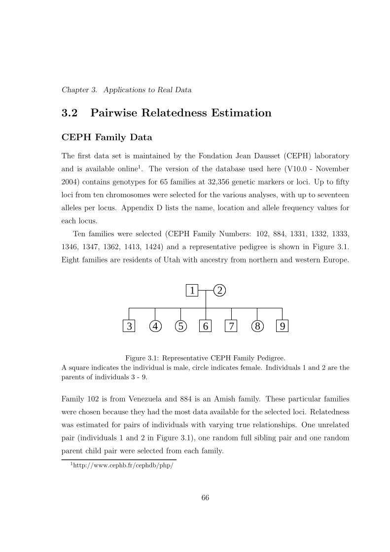
Chapter 3. Applications to Real Data
3.2 Pairwise Relatedness Estimation
CEPH Family Data
The first data set is maintained by the Fondation Jean Dausset (CEPH) laboratory
and is available online1. The version of the database used here (V10.0 - November
2004) contains genotypes for 65 families at 32,356 genetic markers or loci. Up to fifty
loci from ten chromosomes were selected for the various analyses, with up to seventeen
alleles per locus. Appendix D lists the name, location and allele frequency values for
each locus.
Ten families were selected (CEPH Family Numbers: 102, 884, 1331, 1332, 1333,
1346, 1347, 1362, 1413, 1424) and a representative pedigree is shown in Figure 3.1.
Eight families are residents of Utah with ancestry from northern and western Europe.
1 2
4 5 83 6 7 9
1 22
4 5 83 6 7 9
Figure 3.1: Representative CEPH Family Pedigree.
A square indicates the individual is male, circle indicates female. Individuals 1 and 2 are the
parents of individuals 3 - 9.
Family 102 is from Venezuela and 884 is an Amish family. These particular families
were chosen because they had the most data available for the selected loci. Relatedness
was estimated for pairs of individuals with varying true relationships. One unrelated
pair (individuals 1 and 2 in Figure 3.1), one random full sibling pair and one random
parent child pair were selected from each family.
1http://www.cephb.fr/cephdb/php/
66
This document is a research report submitted to the U.S. Department of Justice. This report has not been published by the Department. Opinions or points of view expressed are those of the author(s) and do not necessarily reflect the official position or policies of the U.S. Department of Justice.

Chapter 3. Applications to Real Data
Results
Continuous Estimation of Relatedness. The maximum likelihood techniques de-
scribed in Section 2.3 were used to obtain maximum likelihood estimators (MLEs) of
the coancestry coefficient (θXY ). The two, six, and eight dimensional MLE values for
the unrelated pairs of individuals are plotted in Figure 3.2. Based on twenty loci, two
50 Loci
0.00
0.03
0.06
0.09
0.12
102 884 1331 1332 1333 1346 1347 1362 1413 1424
Family
θ XY M
LE
2D MLE 6D MLE 8D MLE
20 Loci
0.00
0.03
0.06
0.09
0.12
102 884 1331 1332 1333 1346 1347 1362 1413 1424
Family
θ XY
ML
E
Figure 3.2: 2D, 6D and 8D MLEs for Unrelated CEPH Individuals, based on 20 or 50 loci.
families (102 and 1331) appear to have higher estimated relatedness than would be
expected for unrelated individuals. As we increase loci, the estimates decrease, but
family 102 still has particularly large estimates. Another anomaly occurs in the 8D
MLE when increasing the number of loci. Several families estimates actually increase;
884, 1346, 1362, 1413. Assuming no inbreeding, the biases should be getting smaller
(estimates getting closer to zero) as the number of loci increase. More investigation is
needed to determine the cause of these inflated estimates.
The variability of the MLEs can be estimated using a bootstrap technique. For
each pair of individuals, 1000 bootstrap samples were generated by randomly selecting
the corresponding number of loci, without replacement. For each bootstrap sample,
the MLE was obtained using the three different methods. The variance of these MLEs
approximates the true variance of the estimate. Table 3.1 shows the MLE, estimated
variances, and bootstrap confidence intervals for the unrelated pairs from families 102
67
This document is a research report submitted to the U.S. Department of Justice. This report has not been published by the Department. Opinions or points of view expressed are those of the author(s) and do not necessarily reflect the official position or policies of the U.S. Department of Justice.

Chapter 3. Applications to Real Data
and 1331. The bootstrap confidence interval endpoints are the fifth and ninety-fifth
Table 3.1: 2D, 6D and 8D MLEs, Bootstrap (BS) Standard Errors and 90% BS CIs.
Husband wife pairs from CEPH families 102 and 1331. 1000 BS replicates were generated in
each case.
Family 102 Family 1331
Method Loci MLE (BS SE) BS CI MLE (BS SE) BS CI
2P 20 0.0887 (0.0584) (0.0021, 0.2038) 0.0467 (0.0418) (0.0000, 0.1359)50 0.0494 (0.0418) (0.0000, 0.1276) 0.0209 (0.0246) (0.0000, 0.0693)
6P 20 0.0881 (0.0600) (0.0109, 0.2164) 0.0531 (0.0454) (0.0007, 0.1426)50 0.0550 (0.0380) (0.0031, 0.1297) 0.0121 (0.0252) (0.0003, 0.0802)
8P 20 0.1028 (0.0589) (0.0319, 0.2339) 0.0562 (0.0447) (0.0113, 0.1549)50 0.0573 (0.0352) (0.0131, 0.1266) 0.0305 (0.0260) (0.0047, 0.0860)
percentile values of the 1000 bootstrap MLEs obtained in each case. Each estimation
method provides similar results. In all cases, increasing the number of loci tends to
decrease the MLE value by about half. It also reduces the width of the confidence
interval by about half. The standard errors for all three estimators are similar, and
are reduced by increasing the number of loci. It is important to note that the results
for these families are extreme. The average 20 loci CI lengths for the other eight
families were 0.0450, 0.0626, and 0.0894, for the 2D, 6D, and 8D estimation methods,
respectively. In the 50 loci case, these average lengths reduced to 0.0128, 0.0297, and
0.0591.
Plotting the estimated values of P0 versus P1 is a more informative way to visualize
the results. Recall, from Section 2.1, the measures P0, P1, and P2. They represent
the probability that two individuals share 0, 1, or 2 alleles identical by descent (IBD),
respectively. These values can be expressed as functions of Jacquard’s coefficients,
P0 = ∆2 + ∆4 + ∆6 + ∆9,
P1 = ∆3 + ∆5 + ∆8,
P2 = ∆1 + ∆7,
68
This document is a research report submitted to the U.S. Department of Justice. This report has not been published by the Department. Opinions or points of view expressed are those of the author(s) and do not necessarily reflect the official position or policies of the U.S. Department of Justice.

Chapter 3. Applications to Real Data
and as functions of the seven parameter model φ-coefficients,
P0 = φ2 + φ4 + φ7,
P1 = φ3 + φ8,
P2 = φ1 + φ7.
The plots for unrelated estimates based on 20 and 50 loci are shown in Figure 3.3. The
true, non-inbred values for any particular relationship are also plotted along with the
estimates. The plot based on 20 loci clearly indicates the husband-wife pair for family
20 Loci
0.0
0.2
0.4
0.6
0.8
1.0
0 0.2 0.4 0.6 0.8 1
P 0
P1
2D MLEs 6D MLEs 8D MLEs True Values
102102102
50 Loci
0.0
0.2
0.4
0.6
0.8
1.0
0 0.2 0.4 0.6 0.8 1P 0
P1
102102
102
Full Siblings
Parent-Child
Cousins
Unrelated
Figure 3.3: P0 versus P1 Plots for Unrelated CEPH Individuals.
102 are highly related. In fact, all MLEs fall in between the true values for cousins and
full siblings. The plot based on 50 loci indicates a lesser relationship, as the plotted
values now fall between unrelated and cousins. Thus, increasing the number of loci
has reduced the estimated relatedness for families 102 and 1331. More investigation is
needed (increasing the numbers of loci) to determine if the husband and wife pairs for
these two families are in fact related.
Plots of full sibling and parent child pair MLE estimates and their associated boot-
strap confidence intervals appear in Figure 3.4. In each family, one sibling pair and
one parent child pair were randomly selected, and the estimates are based on fifty loci.
In most of the full sibling cases, the true value for θXY falls within the bounds of the
69
This document is a research report submitted to the U.S. Department of Justice. This report has not been published by the Department. Opinions or points of view expressed are those of the author(s) and do not necessarily reflect the official position or policies of the U.S. Department of Justice.

Chapter 3. Applications to Real Data
0 0.1 0.2 0.3 0.4 0.5
Full Siblings (50 Loci)
True Value
Fam
ily
Nu
mbe
r
0 0.1 0.2 0.3 0.4 0.5
MLE Value2D6D8D884-21331-21332-21333-21346-21347-21362-21413-21424-2884-61331-61332-61333-61346-61347-61362-61413-61424-6884-81331-81332-81333-81346-81347-81362-81413-81424-8True Value
Parent Child (50 Loci)
True Value
102
884
1331
1332
1333
1346
1347
1362
1413
1462
Figure 3.4: 2D, 6D and 8D MLEs for Full Sibling and Parent Child CEPH Pairs
Based 50 loci, interval around MLE values based on 1000 bootstrap samples. True value
based on the assumption of no inbreeding.
bootstrap CIs. The major exception occurs with the pair from family 884. The 2D,
6D, and 8D estimates in this case were 0.0705, 0.0706, and 0.0749. More investigation
is needed here to determine if these individuals are actually siblings. It worth enter-
taining the idea that perhaps they are half siblings, and the CEPH database entries
were incorrect. For most of the full sibling pairs the three estimates were very similar,
and tend to underestimate the true relationship. The average biases over families (ex-
cluding family 884), were -0.0164, -0.0189, and -0.0095 for the 2D, 6D, and 8D MLEs
70
This document is a research report submitted to the U.S. Department of Justice. This report has not been published by the Department. Opinions or points of view expressed are those of the author(s) and do not necessarily reflect the official position or policies of the U.S. Department of Justice.

Chapter 3. Applications to Real Data
respectively. The average CI lengths were also very similar: 2D = 0.1402, 6D=0.1583,
8D=0.1582.
The plot in Figure 3.4 based on parent child pairs clearly show the advantages of
reducing the number of parameters in the model. Both the 2D and 6D methods are
performing quite well, whereas the 8D method is showing less reliable results. The
8D estimator is showing large biases, and the MLE values tend to lie closer to the
endpoints of the CIs. This effect does is not evident in the 2D and 6D cases These
plots also help show the performance of all three estimators is highly dependent on the
true relationship. The CIs for the 2D and 6D estimates were much smaller than those
observed for full sibs (averages were 0.0331 and 0.1060 respectively). This reduction
in CI length was not observed for the 8D estimate, as the average length increased to
0.1747. The true value of θXY is contained in the CIs for every family.
Based on these results, we conclude the 8D estimator is more biased and exhibits
higher standard errors than the 2D counterpart. The increase in variance can be
attributed to the large number of estimates required for the 8D estimator. This could
also affect the bias, as in the non-inbred case the true values for ∆1, . . . ,∆6 are zero,
regardless of the true relationship. Thus, we have increased the dimensionality when
in fact it was unnecessary. When the number of parameters is reduced to six, some
improvement was seen when the true relationships were unrelated and parent child.
Based on the estimates obtained here, the parents of family 102 are more related than
we would expect. In this case, the 8D and 6D methods for full sibs and parent-child
will be more accurate. For example, one full sib pair from this family had a 2D MLE
of 0.2234, a 6D MLE of 0.2424, and an 8D MLE of 0.2754. If we set the inbreeding
coefficient equal to 0.09 (the smaller estimated relatedness between individuals 1 and
2) the true value of θXY is 0.3175. Thus, the 8D MLE is much closer to the true value
than the 2D MLE.
Discrete Estimation of Relatedness. The classification techniques described in
Section 2.3 were used to obtain discrete estimates of relatedness. The two, six, and
71
This document is a research report submitted to the U.S. Department of Justice. This report has not been published by the Department. Opinions or points of view expressed are those of the author(s) and do not necessarily reflect the official position or policies of the U.S. Department of Justice.

Chapter 3. Applications to Real Data
eight dimensional accuracy rates for unrelated, full sib, and parent-child pairs are
shown in Figure 3.5. The 10 unrelated pairs are simply the husband-wife pairs from
20 Loci
0
0.2
0.4
0.6
0.8
1
Unrelated Full Siblings Parent Child
Acc
urac
y R
ates
2D MLE 6D MLE 8D MLE
50 Loci
0
0.2
0.4
0.6
0.8
1
Unrelated Full Siblings Parent Child
Figure 3.5: CEPH Data Accuracy Rates for 2D, 6D and 8D Discrete Relatedness Estimates.
The rates are based on 10 unrelated pairs, 50 full sibling pairs, and 50 parent-child pairs.
each family. The five full sibling and five parent child pairs were randomly chosen from
each family, giving rise to 50 observations in those cases. The accuracy rates based on
twenty loci are relatively high with the exception of the 8D rate for parent-child pairs.
In this case, 29 out of the 50 pairs were misclassified as full sibling pairs, and one pair
was misclassified as unrelated. These, for the most part, were evenly spread among
the 10 families. The exception was family 102, where 4 of the 5 parent-child pairs were
misclassified. Again, this is most likely due to the high relatedness observed between
the parents. Overall, it is difficult to conclude from these results which method proved
more accurate. A similar statement can be made concerning the results from 50 loci.
Accuracy rates do improve in every category, but which one is “best” is still not clear.
The 6D and 8D methods work well for full siblings, but the 2D method is superior
for parent-child pairs. Overall, the 6D method provides adequate results, even in the
non-inbred case.
As a final note, recall that all estimates reported here are based on only 20 or 50
loci. According to the simulation results provided in Chapter 2, these numbers are not
sufficient to expect accurate estimators. As such, the results stated here are tentative
72
This document is a research report submitted to the U.S. Department of Justice. This report has not been published by the Department. Opinions or points of view expressed are those of the author(s) and do not necessarily reflect the official position or policies of the U.S. Department of Justice.

Chapter 3. Applications to Real Data
and need further verification using more loci.
FBI Data
Another data set available online is provided by the FBI2. Genotypes at several loci are
provided for samples obtained from six different human populations; 210 US African
Americans (AA), 162 Bahamians (BA), 244 Jamaicans (JA), 209 US Hispanics (HI),
85 Trinadadians (TR) and 203 US Caucasians (CA). All samples were genotyped at
the thirteen CODIS3 loci. In addition, the African American, Caucasian, and Hispanic
samples were also typed for the loci HLA-DQA1, LDLR, GYPA, HBGG, D7S8, Gc,
and D1S80. The number of alleles per locus vary from 2 to 28. Allele frequencies were
estimated from each population separately, using all observations from each sample.
Within each sample, 500 randomly selected pairs comprised the unrelated data set.
Additionally, 500 random pairs were selected and “mated” to obtain parent-child pairs
and full sibling pairs.
Results
Continuous Estimation of Relatedness. If we assume no population substruc-
ture exists in these six populations, all three estimators are biased high (Figure 3.6).
In most cases, the biases observed for the 8D and 6D MLEs were much larger than
those observed for the 2D MLE. The most extreme difference occurred when the true
relationship was parent child. Reducing the dimensionality from eight to six did not
have an effect on the biases, as few differences exist between the 6D and 8D MLE.
Since pairs are “mated” to arrive at full sibling and parent child pairs, the variability
can be estimated by computing the standard deviation of the 500 estimates in each
case. This is in contrast to the bootstrap technique used for the CEPH data, where
we were relying on the data to determine true relationships. The standard deviations
2http://www.fbi.gov/hq/lab/fsc/backissu/july1999/budowle.htm3See http://www.fbi.gov/hq/lab/codis/ for more information about the FBI’s CODIS program.
73
This document is a research report submitted to the U.S. Department of Justice. This report has not been published by the Department. Opinions or points of view expressed are those of the author(s) and do not necessarily reflect the official position or policies of the U.S. Department of Justice.

Chapter 3. Applications to Real Data
0.00
0.02
0.04
0.06
0.08
AA BA JA HI TR CA
Ave
rage
Bia
s
2D MLE 6D MLE 8D MLE
AA BA JA HI TR CA AA BA JA HI TR CA
Full SiblingsUnrelated Parent Child
Population Population Population
Figure 3.6: Plotted Biases of the 2D, 6D and 8D MLEs, FBI Data.
Each plot based on 500 observations, biases were calculated assuming no population sub-
structure
for each case are shown in Figure 3.7. The standard deviations are very similar across
0.00
0.01
0.02
0.03
0.04
AA BA JA HI TR CA
Stan
dard
Dev
iatio
ns
2D MLE 6D MLE 8D MLE
AA BA JA HI TR CA AA BA JA HI TR CA
Full SiblingsUnrelated Parent Child
Population Population Population
Figure 3.7: Plotted Standard Deviations of the 2D, 6D and 8D MLEs, FBI Data.
Each plot based on 500 observations.
estimators in the unrelated and full sibling cases. The 2D MLE shows much smaller
values in the parent child case. The variation between populations appears to be a
direct function of the bias. For example, the Jamaican sample showed the highest
MLE values and they also display the highest standard deviations.
74
This document is a research report submitted to the U.S. Department of Justice. This report has not been published by the Department. Opinions or points of view expressed are those of the author(s) and do not necessarily reflect the official position or policies of the U.S. Department of Justice.

Chapter 3. Applications to Real Data
If the no population structure assumption is incorrect, then the bias for the 8D
and 6D MLEs would be reduced. In [49], Weir and Hill calculated single-population
estimates of the inbreeding coefficient for three of the six populations, based on the 13
CODIS loci: African American, ψ = 0.010; Caucasian, ψ = 0.017; Hispanic, ψ = 0.032.
The biases were recalculated for the 2D and 8D estimates, using these estimated in-
breeding coefficients, and are presented in Table 3.2. The 6D MLE is not included
Table 3.2: Biases and Standard Errors for the 2D and 8D MLEs, FBI Data.
Each estimate is based on 500 observations. Biases were calculated assuming inbreeding
coefficients of 0.010, 0.017, 0.032 for the AA, CA, and HI samples, respectively. Standard
deviations are given in parentheses.
Unrelated Full Siblings Parent-Child
2D 8D 2D 8D 2D 8D
AA 0.022(0.040) 0.037(0.050) -0.001(0.065) 0.021(0.074) 0.007(0.023) 0.038(0.049)
CA 0.010(0.034) 0.022(0.041) -0.020(0.061) 0.000(0.072) -0.011(0.019) 0.020(0.045)
HI -0.004(0.037) 0.010(0.043) -0.008(0.065) 0.013(0.073) -0.002(0.019) 0.030(0.051)
in this table, as the estimates are very similar to the 8D case. The biases for both
estimators have been reduced by accounting for population substructure. When using
the 2D MLE, the biases are mostly negative confirming the simulation results provided
in Chapter 2. The standard deviations are highest for full siblings, though not by a sig-
nificant amount. The 2D standard deviations are approximately 0.01 less than the 8D
standard deviations in all cases except for parent-child. Here, the standard deviations
for the 8D MLE are at least twice the size of the 2D MLE standard deviations.
To examine the variability and bias of the estimates further, consider the P0 versus
P1 plots shown in Figure 3.8 for the African American sample. These plots show clearly
the additional variation in both the six and eight dimensional MLEs, when compared
to the 2D MLE. In the non-inbred case, parent-child pairs must share one allele IBD.
Thus, the probability of sharing zero alleles is alway zero in the 2D case. With the 6D
and 8D MLE, this is not the case. For example, the probability of zero alleles IBD in
75
This document is a research report submitted to the U.S. Department of Justice. This report has not been published by the Department. Opinions or points of view expressed are those of the author(s) and do not necessarily reflect the official position or policies of the U.S. Department of Justice.

Chapter 3. Applications to Real Data
the 8D case consists of several IBD patterns (S2, S4, S6, S9 from Chapter 2, Table 2.3),
all of which could have probability greater than zero, if population substructure exists.
This causes the extra variation seen in the higher dimension P0 versus P1 plots, and
their MLEs. For this reason, if no inbreeding is suspected we recommend using the 2D
MLE.
Figure 3.8 also demonstrates the advantages of techniques estimating more than one
parameter. Recall from Figure 3.7 that the 6D and 8D θXY estimates displayed very
similar standard deviations. Thus, if the estimates were only one dimensional (like the
moment estimators of Chapter 2) we would conclude both estimates are equally biased
and have similar variability. However, different conclusions would be drawn based on
the two dimensional P0-P1 plots. They show many 8D estimates falling in the full
sibling range, whereas the 6D estimates are more confined to the parent child range.
Thus we would conclude that the 6D method is in fact superior to the 8D method,
0.0
0.2
0.4
0.6
0.8
1.0
0 0.2 0.4 0.6 0.8 1
P 0
P1 Full Siblings
Parent-Child
Cousins
Unrelated
2D MLE
0.0
0.2
0.4
0.6
0.8
1.0
0 0.2 0.4 0.6 0.8 1
P 0
P1
6D MLE
0.0
0.2
0.4
0.6
0.8
1.0
0 0.2 0.4 0.6 0.8 1
P 0
P1
8D MLE
Figure 3.8: P0 versus P1 Plots for Simulated Parent-Child Pairs from AA Sample.
76
This document is a research report submitted to the U.S. Department of Justice. This report has not been published by the Department. Opinions or points of view expressed are those of the author(s) and do not necessarily reflect the official position or policies of the U.S. Department of Justice.

Chapter 3. Applications to Real Data
with respect to both bias and variability.
Discrete Estimation of Relatedness. Figure 3.9 presents the accuracy rates, av-
eraged over the 6 populations. The results here are very similar to those obtained
0
0.2
0.4
0.6
0.8
1
Unrelated Full Siblings Parent Child
Ave
rage
Acc
urac
y R
ates
2D MLE 6D MLE 8D MLE
Figure 3.9: Mean Accuracy Rates for FBI Data.
Means were obtained by averaging all accuracy rates obtained for the six samples.
for the CEPH data set, except the 8D accuracy rates are higher. Table 3.3 provides
individual accuracy rates for each of the six samples. As in the CEPH example, the
Table 3.3: Individual Accuracy Rates for FBI Data.
Unrelated Full Siblings Parent-Child
Sample 2D 6D 8D 2D 6D 8D 2D 6D 8D
AA 0.890 0.900 0.896 0.816 0.842 0.878 0.914 0.834 0.704
BA 0.902 0.888 0.886 0.782 0.814 0.864 0.782 0.820 0.668
JA 0.840 0.808 0.806 0.704 0.758 0.788 0.704 0.738 0.626
HI 0.932 0.926 0.922 0.786 0.810 0.846 0.786 0.842 0.712
TR 0.906 0.860 0.864 0.792 0.818 0.848 0.792 0.798 0.708
CA 0.940 0.924 0.940 0.806 0.840 0.882 0.806 0.848 0.720
accuracy rates are relatively high for most cases, considering only twenty loci were
77
This document is a research report submitted to the U.S. Department of Justice. This report has not been published by the Department. Opinions or points of view expressed are those of the author(s) and do not necessarily reflect the official position or policies of the U.S. Department of Justice.
Chapter 3. Applications to Real Data
used. The estimator with the highest accuracy varies between populations and true
relationships. The accuracy rates for all methods are affected by the increased variabil-
ity evident in the MLEs for the Jamaican sample. The lower rates for the 8D estimate
in the parent-child case are most likely due to the additional variation observed in the
8D MLE (see Figure 3.8). Again, it is difficult to conclude from these results which
method is more accurate. The next data set provides genetic data on a large number
of loci, and should thus provide less ambiguous results.
HapMap Data
The International HapMap Project is a multi-country effort to genotype humans from
several populations [50]. The samples are from a total of 209 individuals, including 60
Yoruba people in Ibadan, Nigeria, 44 Japanese in Tokyo, 45 Han Chinese in Beijing,
and 60 Americans from the CEPH families previously mentioned. The amount of
data the HapMap Consortium has made available is massive. We consider here only
observations from loci on chromosome 2. There are a total of 54,649 equally spaced loci
typed, each with two alleles. In this study, we use every 100th locus, for a total of 547
loci. Allele frequencies were again estimated from each individual sample. Unrelated,
parent-child, and full sib pairs were generated using the same methods as for the FBI
data set, taking care that repeat pairs did not occur.
Results
Continuous Estimation of Relatedness. Plots of the biases, assuming no popu-
lation structure are shown in Figure 3.10. First note the drastic reduction in bias for
this data set, as compared to the biases for the FBI data set given in Figure 3.6. For
example, for unrelated pairs, the 2D MLE biases ranged between 0.02 and 0.05. With
the increase in loci, the range is now reduced to (0.006, 0.008). Similar results are seen
with the 6D and 8D MLEs. It is encouraging to see these results, considering there are
only 2 alleles per locus. In most cases the 6D and 8D MLEs are still displaying higher
78
This document is a research report submitted to the U.S. Department of Justice. This report has not been published by the Department. Opinions or points of view expressed are those of the author(s) and do not necessarily reflect the official position or policies of the U.S. Department of Justice.

Chapter 3. Applications to Real Data
-0.04
-0.02
0.00
0.02
0.04
CEU HCB JPT YRI
2D MLE 6D MLE 8D MLE
CEU HCB JPT YRI CEU HCB JPT YRI
Full SiblingsUnrelated Parent Child
Ave
rage
Bia
ses
Figure 3.10: Plotted Biases of the 2D and 8D MLEs, HapMap Data.
Each plot based on 500 observations, biases were calculated assuming no population sub-
structure.
biases than the 2D estimate, as population substructure is not suspected in these pop-
ulations. In the full sibling case however, the 6D MLE is actually underestimating
θXY . These biases are small, and range from -0.009 to -0.003.
Increasing the number of loci also had an impact on the amount of variation seen
in the estimates. Table 3.4 gives the standard deviation values for two samples, the
FBI African American sample and the HapMap CEU sample. These results confirm
Table 3.4: Standard Errors of the 2D, 6D and 8D MLE for Selected Samples.
Unrelated Full Siblings Parent-Child
Sample 2D 6D 8D 2D 6D 8D 2D 6D 8D
FBI(AA) 0.040 0.046 0.294 0.065 0.069 0.074 0.023 0.044 0.049
HAP (CEU) 0.012 0.011 0.011 0.020 0.030 0.023 0.006 0.019 0.023
that increasing the number of loci, even if they are biallelic, increases all estimators’
accuracy and precision. Next, we consider the impact of increasing loci on the discrete
estimation of relationships.
79
This document is a research report submitted to the U.S. Department of Justice. This report has not been published by the Department. Opinions or points of view expressed are those of the author(s) and do not necessarily reflect the official position or policies of the U.S. Department of Justice.

Chapter 3. Applications to Real Data
Discrete Estimation of Relatedness. When estimating discrete relatedness every
relationship was estimated with at least 90% accuracy using all three methods. The
accuracy rates averaged over populations appear in Figure 3.11. The lowest values
0
0.2
0.4
0.6
0.8
1
Unrelated Full Siblings Parent Child
Ave
rage
Acc
urac
y R
ates
2D MLE 6D MLE 8D MLE
Figure 3.11: Mean Accuracy Rates for Hapmap Data.
Means were obtained by averaging all accuracy rates obtained for the four samples.
obtained were 0.908 (8D, Parent Child, HI data) and 0.92 (6D, Parent Child, AA and
BA data). All cases showed drastic improvement from the accuracy using the FBI data
set. Consider the two P0 versus P1 plots for the CEU sample shown in Figure 3.12.
In the first plot, there are distinct clusters for each of the groups. In addition, within
each cluster, the observations are all closest to the appropriate true relationship value.
This is not the case in the second two plots. Similar to the results shown in Figure 3.8,
we see quite a bit of scatter when the true relationship is parent child. Several 8D
observations are still closer to the true value for full siblings than parent-child.
The results we have shown here have assumed that there were only three possible
relationship categories: unrelated, full sibling, and parent-child. However, there are
realistic circumstances where the number of categories will be more than three. As
such, we obtained accuracy rates for the case when there are five possible relationship
types: unrelated, cousins, half siblings, full siblings, and parent-child. These results
are summarized in Table 3.5. Increasing the number of alternatives did not impact
80
This document is a research report submitted to the U.S. Department of Justice. This report has not been published by the Department. Opinions or points of view expressed are those of the author(s) and do not necessarily reflect the official position or policies of the U.S. Department of Justice.

Chapter 3. Applications to Real Data
0.0
0.2
0.4
0.6
0.8
1.0
0 0.2 0.4 0.6 0.8 1
P 0
P1
Full Siblings
Parent-Child
Cousins
Unrelated
2D MLE
0.0
0.2
0.4
0.6
0.8
1.0
0 0.2 0.4 0.6 0.8 1
P 0
P1
6D MLE
0.0
0.2
0.4
0.6
0.8
1.0
0 0.2 0.4 0.6 0.8 1
P 0
P1
8D MLE
Figure 3.12: P0 versus P1 Plots for Simulated Pairs from CEU Sample.
Table 3.5: Individual Accuracy Rates for HapMap Data.
These results were obtained by considering five different relationship types, instead of three.
Unrelated Full Siblings Parent-Child
Sample 2D 6D 8D 2D 6D 8D 2D 6D 8D
CEU 0.976 0.968 0.966 0.972 0.958 0.752 1.000 0.920 0.930
HCB 0.974 0.972 0.970 0.982 0.954 0.728 1.000 0.920 0.944
JPT 0.982 0.970 0.972 0.964 0.972 0.802 1.000 0.938 0.946
YRI 0.966 0.954 0.948 0.980 0.956 0.760 1.000 0.930 0.908
the accuracy of the 2D estimator significantly. The 2D classification method is now at
least 96% accurate, whereas in the three alternative case it was at least 98% accurate.
However, there was a large impact on the 8D estimator for full sibling case. This is
due to the additional scatter that is seen in the 8D P0 versus P1 plots in Figure 3.12.
81
This document is a research report submitted to the U.S. Department of Justice. This report has not been published by the Department. Opinions or points of view expressed are those of the author(s) and do not necessarily reflect the official position or policies of the U.S. Department of Justice.

Chapter 3. Applications to Real Data
Reductions in accuracy also occurred with the 6D method for full siblings, although
not as extreme. Both full sibs and unrelated pairs were most commonly misclassified
as cousins (detailed results for the 8D full sibling case are given in Figure 3.13). A
reduction in the accuracy in the parent-child case was not seen, as no other competing
relationship was added that is closer than full siblings to the parent child space.
0
0.2
0.4
0.6
0.8
1
Unrelated Cousins Half Siblings Full Siblings Parent Child
Acc
urac
y R
ates
CEU HCB JPT YRI
Figure 3.13: Classification Rates for the 8D Method when True Relationship is Full Sibling.
To conclude, the 2D method of classification is very accurate when large numbers of
loci are given. They provides results that are over 97% accurate in every case considered
here. Future studies are needed before the 6D and 8D estimators can be recommended
for forensic uses. First, one should investigate whether or not the accuracy for parent-
child improves with larger number of alleles per locus. In addition, studies such as
those performed here should be conducted with real data that is known to have a
large inbreeding coefficient. Studies such as these would help determine if the best
discrete estimator to use depends upon population substructure, which it most likely
will. Finally, simulation studies should be done comparing the discrete estimators
discussed here with other existing methods of relationship classification.
82
This document is a research report submitted to the U.S. Department of Justice. This report has not been published by the Department. Opinions or points of view expressed are those of the author(s) and do not necessarily reflect the official position or policies of the U.S. Department of Justice.

Chapter 3. Applications to Real Data
3.3 Multiple Allele Paternity Network Example
The Bayesian Network (BN) examples considered in Chapter 1 used data from only
one locus. We present here a more realistic example. Consider family 102 from the
CEPH data set. From the analyses performed in the previous section, we have reason
to believe this family has an inbreeding coefficient (ψ) greater than zero. Thus, this
family would be an interesting case to consider for the BN described in Example Two
from Chapter 1 (Figure 1.11). The genotypes for the mother and child (individual 3)
are available at 19 loci (the mother’s genotype is missing for locus GATA41A01). We
can then suppose the “putative” father is individual 1 (the actual father) and use the
BN to calculate paternity indices (PIs) for each locus.
For this example, we set the inbreeding coefficient to be 0.0917, the 2D MLE for the
coancestry coefficient between the mother and putative father. The PI for each locus
was also calculated using a non-population substructure network, which assumes ψ = 0.
The genotypes and PIs for each locus are provided in Table 3.6. Assuming these loci are
independent, the overall paternity index is obtained by multiplying all of the individual
PI values. When ψ = 0.0917, the overall PI is 22405 and when ψ = 0 the PI is 551,758.
Both PIs are large and either case would lead us to conclude that the putative father
is the father of the child in question. However, when population structure is ignored
the overall PI is about 25 times larger. In certain circumstances, this overestimation
could lead to an incorrect statement about paternity. This example helps demonstrate
the high dependence of the PI upon the population substructure assumptions. Thus,
if there is evidence to conclude that there is a moderate amount of substructure, the
BN of Figure 1.11 should be employed.
Approximately one hour was needed to enter in the allele frequencies, genotypes,
and to obtain the output from HUGIN using the population substructure network.
This is in contrast to the twenty minutes needed for the non-population substructure
network. In practice, both of these times are inadequate. These calculations can be
done using existing software in a matter of seconds. Before Bayesian Networks can be
83
This document is a research report submitted to the U.S. Department of Justice. This report has not been published by the Department. Opinions or points of view expressed are those of the author(s) and do not necessarily reflect the official position or policies of the U.S. Department of Justice.

Chapter 3. Applications to Real Data
Table 3.6: CEPH Family 102 Genotypes and PI Values.
The genotypes are given by pairs of allele numbers, where the numbers correspond with
Appendix D. Paternity index (PI) values were obtained using the Bayesian Nework in Fig-
ure 1.11.
Genotypes PI
Locus Chr. P. Father Mother Child ψ = 0 ψ = 0.0917
ATA1G10 8 32 32 32 1.13 1.09
CEB42 8 12 34 23 2.00 2.00
FB12B7 8 56 22 25 1.91 1.93
GATA23C09 8 31 22 32 1.57 1.68
MFD159A 8 17 37 13 6.16 3.85
GATA27G11 12 31 11 31 1.40 1.53
LMS43 12 12 13 13 1.33 1.03
MFD84 12 13 15 15 1.55 1.12
PTHIZ53 12 22 22 22 1.21 1.14
ACT1A01 18 42 55 52 3.26 2.76
AFM123YA1 18 12 23 23 1.02 0.88
ATA1H06 18 52 56 62 17.66 5.43
GATA28D12 18 32 32 32 2.21 1.64
GATA30C02 18 43 44 43 0.95 1.12
MFD302 18 13 13 33 3.44 2.02
CYP2DP8 22 12 13 12 1.70 1.78
GCT10C10 22 11 14 14 1.49 1.31
IL2RB 22 12 11 12 1.30 1.45
PH41A 22 24 22 24 2.69 2.45
widely accepted and used by forensic scientists, this time constraint must be addressed.
One simple solution would be to automate the data entry. If HUGIN could read in
genotypes and allele frequencies from a data file and then perform the appropriate
calculations, the time needed would be greatly reduced. Additional time would be
saved if HUGIN could output the results into another data file. This is one area that
needs more research, in collaboration with BN software providers.
84
This document is a research report submitted to the U.S. Department of Justice. This report has not been published by the Department. Opinions or points of view expressed are those of the author(s) and do not necessarily reflect the official position or policies of the U.S. Department of Justice.

Chapter 3. Applications to Real Data
3.4 Discussion
When estimating pairwise relatedness, we have shown that accounting for substructure
is possible. In fact, the methodology does not differ substantially from methods already
in use. We provided a very simple extension from a two dimensional maximization
problem to a six or eight dimensional problem. The first two data sets considered here
have helped to demonstrate the need for a large number of loci for both methods. The
HapMap Consortium projects 6.8 million single nucleotide polymorphisms or SNPs,
each with a unique genomic position, will be genotyped for a total of 270 individuals
included in their study [50]. The vast majority of these SNPs are biallelic. Recent
technology advances allow genotyping of large samples of individuals at thousands of
SNP loci [51]. The results presented here using a subset of the HapMap data showed
that SNP data is sufficient to accurately estimate pairwise relatedness, especially when
we can assume no population substructure exists (2D MLE).
Bayesian Networks are commonly used to calculate various probabilities from foren-
sic genetic data. We have shown that accounting for substructure is possible. In addi-
tion, the resultant networks are not significantly more complex than those that already
exist. The real data example provided in this chapter demonstrates the vastly different
results that can be obtained. This example also shows that more research on Bayesian
Networks is needed, primarily to explore reducing data entry time.
85
This document is a research report submitted to the U.S. Department of Justice. This report has not been published by the Department. Opinions or points of view expressed are those of the author(s) and do not necessarily reflect the official position or policies of the U.S. Department of Justice.

Literature Cited
[1] J. Wang. An estimator for pairwise relatedness using molecular markers. Genetics,160:1203–1215, 2002.
[2] I.W. Evett and B.S. Weir. Interpreting DNA Evidence. Sinauer, Sunderland,MA., 1998.
[3] A.P. Dawid, J. Mortera, V.L. Pascali, and D. Van Boxel. Probabilistic expert sys-tems for forensic inference from genetic markers. Scandinavian Journal of Statis-tics, 29:577–595, 2002.
[4] J.M. Curran, C.M. Triggs, J. Buckleton, and B.S. Weir. Interpreting DNA mix-tures in structured populations. Journal of Forensic Sciences, 44(5):987–995,1999.
[5] D.J. Balding and R.A. Nichols. A method for quantifying differentiation betweenpopulations at multi-allelic loci and its implications for investigating identity andpaternity. Genetica, 96:3–12, 1995.
[6] D.J. Balding and R.A. Nichols. DNA profile match probability calculation - Howto allow for population stratification, relatedness, database selection and singlebands. Forensic Science International, 64(2–3):125–140, 1994.
[7] N. Fenton and M. Neil. The jury observation fallacy and the use of BayesianNetworks to present probabilistic legal arguments. Mathematics Today, 36(6):180–187, 2000.
[8] R.G. Cowell. FINEX: A probabilistic expert system for forensic identification.Forensic Science International, 134:196–206, 2003.
[9] R.G. Cowell, A.P. Dawid, S.L. Lauritzen, and D.J. Speidelhalter. Probabilis-tic Networks and Expert Systems. Springer-Verlag, Berlin-Heidelberg-New York,1999.
[10] B.S. Weir. Quantifying the genetic structure of populations with application topaternity calculations. In M.E. Halloran and S. Geisser, editors, Statistics inGenetics Volume 112 of IMA Volumes in Mathematics and its Applications, pages31–44. Springer-Verlag, New York, 1998.
86
This document is a research report submitted to the U.S. Department of Justice. This report has not been published by the Department. Opinions or points of view expressed are those of the author(s) and do not necessarily reflect the official position or policies of the U.S. Department of Justice.

Literature Cited
[11] B.S. Weir. Effects of inbreeding on forensic calculations. Annual Review of Ge-netics, 28:597–621, 1994.
[12] J.M. Curran, J.S. Buckleton, and C.M. Triggs. What is the magnitude of thesubpopulation effect? Forensic Science International, 135(1):1–8, 2003.
[13] P. Garbolino and F. Taroni. Evaluation of scientific evidence using BayesianNetworks. Forensic Science International, 125(2–3):149–155, 2002.
[14] National Research Council. The Evaluation of Forensic DNA Evidence. NationalAcademy Press, Washington, DC, 1996.
[15] T.S. Levitt and K.B. Laskey. Computational inference for evidential reasoning insupport of judicial proof. Cardozo Law Review, 22:1691–1731, 2001.
[16] I.W. Evett, P.D. Gill, G. Jackson, J. Whitaker, and C. Champod. Interpretingsmall quantities of DNA: the hierarchy of propositions and the use of BayesianNetworks. Journal of Forensic Sciences, 47(3):520–530, 2002.
[17] P.E.M. Huygen. Use of Bayesian Belief Networks in legal reasoning. In 17thBILETA Annual Conference, 2002.
[18] A.P. Dawid. An object-oriented Bayesian Network for estimating mutation rates.In Ninth International Workshop on Artificial Intelligence and Statistics, 2003.
[19] C. Aitken, F. Taroni, and P. Garbolino. A graphical model for the evaluation ofcross-transfer evidence in DNA profiles. Theoretical Population Biology, 63:179–190, 2003.
[20] J. Mortera, A.P. Dawid, and S.L. Lauritzen. Probabilistic expert systems for DNAmixture profiling. Theoretical Population Biology, 63:191–205, 2003.
[21] J. Mortera. Analysis of DNA mixtures using Bayesian Networks. In P.J. Green,N.L. Hjort, and S. Richardson, editors, Highly Structured Stochastic System, pages39–44. Oxford University Press, 2003.
[22] J.W. Morris, R.A. Garber, J. d’Autremont, and C.H. Brenner. The avuncularindex and the incest index. Advances in Forensic Haemogenetics 1, pages 607–611, 1988.
[23] M. Lynch and K. Ritland. Estimation of pairwise relatedness with molecularmarkers. Genetics, 152:1753–1766, 1999.
87
This document is a research report submitted to the U.S. Department of Justice. This report has not been published by the Department. Opinions or points of view expressed are those of the author(s) and do not necessarily reflect the official position or policies of the U.S. Department of Justice.

Literature Cited
[24] B. Olaisen, M. Stenersen, and B. Mevag. Identification by DNA analysis of thevictims of the August 1996 Spitsbergen civil aircraft disaster. Nature Genetics,15(4):402–405, 1997.
[25] B. Leclair, C.J. Fregeau, K.L. Bowen, and R.M. Fourney. Enhanced kinship analy-sis and STR-based DNA typing for human identification in mass fatality incidents:The Swissair Flight 111 disaster. Journal of Forensic Sciences, 49(5):939–953,2004.
[26] C.H. Brenner and B.S. Weir. Issues and strategies in the DNA identification ofWorld Trade Center victims. Theoretical Population Biology, 63(3):176–178, 2003.
[27] C.H. Brenner. Some mathematical problems in the DNA identification of Tsunamivictims. Unpubished, June 2005.
[28] C.M. Hsu, N.E. Huang, L.C. Tsai, L.G. Kao, C.H. Chao, A. Linacre, and J.C.-I.Lee. Identification of victims of the 1998 Taoyuan Airbus crash accident usingDNA analysis. International Journal of Legal Medicine, 113(1):43–46, 1999.
[29] C.W. Cotterman. A Calculus for Statistico-Genetics. PhD thesis, Ohio StateUniversity, 1940.
[30] D.C. Queller and K.F. Goodnight. Estimating relatedness using molecular mark-ers. Evolution, 43:258–275, 1989.
[31] M.S. Blouin. DNA-based methods for pedigree reconstruction and kinship analysisin natural populations. Trends in Ecology and Evolution, 18(10):503–511, 2003.
[32] T. Van De Casteele, P. Galbusera, and E. Matthysen. A comparisonof microsatellite-based pairwise relatedness estimators. Molecular Ecology,10(6):1539–1549, 2001.
[33] B.G. Milligan. Maximum likelihood estimation of relatedness. Genetics, 163:1153–1167, 2003.
[34] A. Grafen. A geometric view of relatedness. Oxford Surveys in EvolutionaryBiology, 2:39–89, 1985.
[35] M. Lynch. Estimation of relatedness by DNA fingerprinting. Molecular and Bio-logical Evolution, 5:584–599, 1988.
[36] C.C. Li, D.E. Weeks, and A. Chakravarti. Similarity of DNA fingerprints due tochance and relatedness. Human Heredity, 43:45–52, 1993.
88
This document is a research report submitted to the U.S. Department of Justice. This report has not been published by the Department. Opinions or points of view expressed are those of the author(s) and do not necessarily reflect the official position or policies of the U.S. Department of Justice.

Literature Cited
[37] K. Ritland. Estimators for pairwise relatedness and individual inbreeding coeffi-cients. Genetical Research, 67:175–185, 1996.
[38] O.J. Hardy. Estimation of pairwise relatedness between individuals and char-acterization of isolation-by-distance processes using dominant genetic markers.Molecular Ecology, 12:1577–1588, 2003.
[39] K. Belkhir, V. Castric, and F. Bonhomme. IDENTIX, a software to test forrelatedness in a population using permutation methods. Molecular Ecology, 2:611–614, 2002.
[40] E.A. Thompson. The estimation of pairwise relationships. Annals of HumanGenetics, 39:173–188, 1975.
[41] E.A. Thompson and T.R. Meagher. Genetic linkage in the estimation of pairwiserelationship. Theoretical and Applied Genetics, 97:857–864, 1998.
[42] M. McPeek and L. Sun. Statistical tests for detection of misspecified relationshipsby use of genome-screen data. American Journal of Human Genetics, 66:1076–1094, 2000.
[43] E.A. Thompson. Estimation of relationships from genetic data. In C.R. Rao andR. Chakraborty, editors, Handbook of Statistics, Vol. 8, pages 225–269. ElsevierScience Publishers, 1991.
[44] A. Jacquard. Genetic information given by a relative. Biometrics, 28:1101–1114,1972.
[45] W.H. Press, S.A. Teukolsky, W.T. Vetterling, and B.P. Flannery. NumericalRecipes in C: The Art of Scientific Computing. Cambridge University Press, Cam-bridge, UK., 1992.
[46] J.A. Nelder and R. Mead. A simplex method for function minimization. ComputerJournal, 7(4):308–313, 1965.
[47] C.H. Brenner. Kinship analysis by DNA when there are many possibilities. InProgress in Forensic Genetics 8, 1999.
[48] C.H. Brenner. Symbolic kinship program. Genetics, 145:535–542, 1997.
[49] B.S. Weir and W.G. Hill. Estimating F-statistics. Annual Review of Genetics,36:721–750, 2002.
89
This document is a research report submitted to the U.S. Department of Justice. This report has not been published by the Department. Opinions or points of view expressed are those of the author(s) and do not necessarily reflect the official position or policies of the U.S. Department of Justice.

Literature Cited
[50] The International HapMap Consortium. The International HapMap Project. Na-ture, 426:789–796, 2003.
[51] J.C. Glaubitz, E. Rhodes Jr., and J.A. DeWoody. Prospects for inferring pairwiserelationships with SNPs. Molecular Ecology, 12:1039–1047, 2003.
90
This document is a research report submitted to the U.S. Department of Justice. This report has not been published by the Department. Opinions or points of view expressed are those of the author(s) and do not necessarily reflect the official position or policies of the U.S. Department of Justice.

Appendix A
A Simple Bayesian Network
This example will provide a basic introduction to Bayesian Networks. It is not intended
to provide a realistic example in which a Bayesian Network can be used, but simply
intended to give an illustrative example. Several unrealistic assumptions are made
purely for the sake of simplicity.
To begin, every BN will have a graphical portion which contains nodes and directed
lines. Each node in the graph represents a variable (or an event), and each directed
line describes the associations that may exist between the variables in the graph. To
demonstrate, a very simple example will be presented that has been adapted from
Aitken et al. [19]. Suppose a crime was committed. The police have a suspect, and
have recovered a blood stain from the crime scene. The proposition that the suspect
is the source of the stain (for simplicity we will say this represents guilt), versus the
proposition that the suspect is not the source of the stain (is not guilty) will be ex-
amined, using the evidence provided by the crime stain. To this end, we will calculate
the following likelihood ratio:
LR =Pr(Evidence|Guilty)
Pr(Evidence|NotGuilty). (A.1)
Three nodes (or variables) will be needed in the BN:
Guilty (G) = Proposition that the suspect is guilty
True Match (M) = Evidence of a true match
91
This document is a research report submitted to the U.S. Department of Justice. This report has not been published by the Department. Opinions or points of view expressed are those of the author(s) and do not necessarily reflect the official position or policies of the U.S. Department of Justice.

Appendix A. A Simple Bayesian Network
Reported Match (RM) = Evidence of a reported match
It is important to mention if we have a “true match” this means that the evidentiary
DNA matches exactly to the suspect’s DNA. We are assuming this implies the culprit
and the suspect are one and the same. In practice, this is not a valid assumption. The
culprit and the suspect could match on a particular set of loci, and it still may not be
reasonable to conclude that they are one in the same.
Each of the variables listed above has two different possible states, either yes or
no. This is an over simplified case, and it is important to note that the variables
within a BN can take on binary (as in this example), categorical, or continuous values.
This allows the flexibility to consider various types of evidence within the same BN.
Figure A.1 is the graphical representation of this hypothetical case.
Figure A.1: A Simple Bayesian Network.
The directed lines in this network indicate the relationships between the three
variables. The arrow from Guilty to True Match indicates that the variable True
Match is dependent upon the variable Guilty. In other words, if Guilty takes on
the value of false, the True Match variable must also take on the value false. The
arrow from True Match to Reported Match indicates the same type of relationship.
When there is a true match, the probability of a Reported Match will necessarily
increase, as long as the match reporting mechanism is working correctly. It is important
to note the absence of a relationship between Guilty and Reported Match. The
92
This document is a research report submitted to the U.S. Department of Justice. This report has not been published by the Department. Opinions or points of view expressed are those of the author(s) and do not necessarily reflect the official position or policies of the U.S. Department of Justice.

Appendix A. A Simple Bayesian Network
probability of a reported match should not depend upon the state of Guilty directly,
only indirectly through the variable True Match.
Along with this graphical representation, the BN will also have a numerical repre-
sentation through various conditional and unconditional probability tables. A proba-
bility table will be associated with every node in a graph. If a node is a parent node,
meaning it does not have any arrows pointing to it, then the probabilities will be uncon-
ditional. This means that the probability of each state of this variable does not depend
on the states of any other variables. There is one such node in this example; Guilty.
For this network, the assumption is that the suspect has a 50% chance of being guilty,
and a 50% chance of being innocent. This implies that the prior odds (Probability
Guilty / Probability Not Guilty) of being guilty are 1; a frequentist assumption. If
one were to appeal to Bayesian reasoning, the prior odds could be specified otherwise,
based upon prior information about the suspect. See [2] for a detailed discussion of the
specification of prior odds for likelihood ratio calculations. The assumption we have
made will lead to the unconditional probability table shown in Table A.1.
Table A.1: Unconditional Probability Table for Guilty Node.
Pr(G)Yes 0.50No 0.50
The other two nodes are considered child nodes, as they have arrows pointing to
them. Each will have a conditional probability table associated with it, as they are
both dependent on other nodes in the graph. The True Match node probabilities
will depend on the current state of Guilty. For example, if Guilty takes on the value
93
This document is a research report submitted to the U.S. Department of Justice. This report has not been published by the Department. Opinions or points of view expressed are those of the author(s) and do not necessarily reflect the official position or policies of the U.S. Department of Justice.

Appendix A. A Simple Bayesian Network
false, then the probability of having a true match must be 0. Table A.2 presents the
entire probability table. Note that G indicates Not Guilty.
Table A.2: Conditional Probability Table for True Match Node.
Pr(M |G) Pr(M |G)Yes 1 0No 0 1
The final node to be considered is Reported Match. The probabilities of this node
will depend on the value of True Match. For example, if True Match takes on the
value No, then the probability of Reported Match is determined by the chance that
the reporting tool will present a false positive. In this example, arbitrary assumptions
are made that the chance of reporting a false positive is 2% and the chance of reporting
a false negative is 1%. This is required to differentiate between True Match and
Reported Match. In practice, these numbers are significantly lower if not zero. The
need to incorporate them into this network is a result of the previous assumption that
a true match implies the culprit and the suspect are one in the same. Note that we are
not implying that these are reasonable values, they are simply chosen for illustrative
purposes. These assumptions concerning the match reporting mechanism lead to the
conditional probabilities presented in Table A.3. One can enter the probabilities into
Table A.3: Conditional Probability Table for Reported Match Node.
Pr(RM |M) Pr(RM |M )Yes 0.99 0.02No 0.01 0.98
94
This document is a research report submitted to the U.S. Department of Justice. This report has not been published by the Department. Opinions or points of view expressed are those of the author(s) and do not necessarily reflect the official position or policies of the U.S. Department of Justice.

Appendix A. A Simple Bayesian Network
HUGIN, and the resultant tables are shown in Figure A.2.
Figure A.2: Probability Tables from HUGIN.
The current example requires a calculation of the likelihood ratio shown in Equa-
tion A.1. The evidence mentioned in this equation is replaced with the variable Re-
ported Match. When coupled with the notation G = Not Guilty, the following equation
represents the likelihood ratio:
LR =Pr(RM |G)
Pr(RM |G)(A.2)
To calculate this value, we will make use of the law of total probability, adapted from [2]:
Law of Total Probability
If A1 and A2 are mutually exclusive and exhaustive events, then for any other event
H ,
Pr(H|E) = Pr(H|A1, E) Pr(A1|E) + Pr(H|A2, E) Pr(A2|E).
Now Pr(RM |G) can be calculated:
Pr(RM |G) = Pr(RM |M,G) Pr(M |G) + Pr(RM |M,G) Pr(M |G)
95
This document is a research report submitted to the U.S. Department of Justice. This report has not been published by the Department. Opinions or points of view expressed are those of the author(s) and do not necessarily reflect the official position or policies of the U.S. Department of Justice.

Appendix A. A Simple Bayesian Network
by the law of total probability, as M and M are mutually exclusive and exhaustive
events. Keeping in mind that the variable Reported Match is independent of the
variable Guilty, and that Pr(M |G) = 1 − Pr(M |G), we have
Pr(RM |G) = Pr(RM |M) Pr(M |G) + Pr(RM |M)(1 − Pr(M |G)).
Finally, taking similar steps we find Pr(RM |G):
Pr(RM |G) = Pr(RM |M,G) Pr(M |G) + Pr(RM |M,G) Pr(M |G)
= Pr(RM |M) Pr(M |G) + Pr(RM |M )(1 − Pr(M |G).
(A.3)
The resultant likelihood ratio is
LR =Pr(RM |M) Pr(M |G) + Pr(RM |M )(1 − Pr(M |G))
Pr(RM |M) Pr(M |G) + Pr(RM |M)(1 − Pr(M |G). (A.4)
Given the formula in Equation A.4, and entering the values from the probability tables
above, Equation A.5 results.
LR =0.99 ∗ 1 + 0.02 ∗ 0
0.99 ∗ 0 + 0.02 ∗ 1=
0.99
0.02= 49.5. (A.5)
HUGIN can be used to perform the same calculations in this BN. Figure A.3 is HUGIN’s
display before any evidence is entered. After entering the evidence of obtaining a
Figure A.3: Before Entering the Evidence.
reported match, HUGIN will display the tables shown in Figure A.4. First, note that
96
This document is a research report submitted to the U.S. Department of Justice. This report has not been published by the Department. Opinions or points of view expressed are those of the author(s) and do not necessarily reflect the official position or policies of the U.S. Department of Justice.

Appendix A. A Simple Bayesian Network
Figure A.4: After Entering the Evidence that we have a Reported Match.
the evidence entered is represented by the 100% next to “Yes” in the Reported Match
table. The likelihood ratio is obtained by taking the value shown in the Guilty table
next to “Yes” and dividing it by the value displayed next to “No.”
LR =98.02
1.98= 49.5. (A.6)
This value is the result shown in Equation A.5.
97
This document is a research report submitted to the U.S. Department of Justice. This report has not been published by the Department. Opinions or points of view expressed are those of the author(s) and do not necessarily reflect the official position or policies of the U.S. Department of Justice.
Appendix B
Corrections and Comments on Wang’s
Paper [1]
In a paper published in 2002 by Jinliang Wang [1], there appear to be several mistakes.
To begin, in the third paragraph of page 1204, Wang states “For a marker locus with
n co-dominant alleles indexed by i, j, k, l = 1, 2, . . . , n there would be G = n(n+ 1)/2
possible genotypes and C = n(n+1)[n(n+1)+2]/8 possible combinations of genotypes
for a pair of individuals.” This statement is false. Consider the counter example of n =
3. Then G = 6, therefore C =(
62
)
= 15. However C = 3(3+1)[3(3+1)+2]/8 = 21 6= 15.
Another discrepancy occurs on page 1205, Table 1. There are several probabilities
that are incorrect, namely Pr(ij, ij),Pr(ii, ij),Pr(ij, kl). These same probabilities are
derived by Evett and Weir in [2], pages 112-1151. Noting the definitions for P0, P1,
and P2 given by Equation 4.12 in [2], Table B.1 summarizes the errors found in [1].
As a final note, Wang states
The ML method can be used to distinguish among different relationships.
Though it can also be used to estimate relatedness, it results in much
larger biases and sampling variances that the moment estimators unless the
number of marker loci is unrealistically large...This is perhaps because the
1There is a typographical error in the first equation on page 113 of [2]. It should readP (AiAi, AjAk) = 2(δ0p
2
i pjpk + δabpipjpk)
98
This document is a research report submitted to the U.S. Department of Justice. This report has not been published by the Department. Opinions or points of view expressed are those of the author(s) and do not necessarily reflect the official position or policies of the U.S. Department of Justice.

Appendix B. Corrections and Comments on Wang’s Paper [1]
ideal properties of the likelihood method are asymptotic and apply to large
data sets only...The data set involved in estimating pairwise relatedness is
extremely small, only two individual genotypes.
This statement is incorrect. The asymptotic properties of the maximum likelihood
technique will apply as the number of loci approach ∞, not as the number of individuals
approach ∞.
Table B.1: Mistaken Probabilities in Wang [1].
P0 = 1 − φ− ∆
P1 = φ
P2 = ∆
Weir Wang
Pr(ij, ij) 4P0p2i p
2j + P1pipj(pi + pj) 2p2
i p2j + 1
2φpipj(pi + pj − 4pipj)
Weir = 2(Wang) +2P2pipj +∆pipj(1 − 2pipj)
Pr(ii, ij) 4p3i pj + 2φp2
i pj(1 − 2pi)
Weir = 2(Wang) 2P0p3i pj + P1p
2i pj −4∆p3
i pj
Pr(ij, kl)
Weir = 4(Wang) 4P0pipjpkpl pipjpkpl − φpipjpkpl − ∆pipjpkpl
99
This document is a research report submitted to the U.S. Department of Justice. This report has not been published by the Department. Opinions or points of view expressed are those of the author(s) and do not necessarily reflect the official position or policies of the U.S. Department of Justice.

Appendix C
Downhill Simplex Method C++ Code
C.1 C++ Function Obtaining 8D MLE
void Get8DMLE(double& max, //i-o variable containing maximum likelihood value
double& theta, //i-o variable containing coancestry coefficient MLE
double init[], //input variable containing 8D initial simplex
double lambda, //input variable contianing scaling factor
int loci, //input variable containing number of loci
double d[]) //i-o variable containing Jacquard’s 8D MLE
//global variable
//LikeClass like[NUM_LOCI]; //One likelihood for each locus
{
SimplexClass simplex;
double iter_delta[N+1][N];
double like_values[N+1];
int n_eval=0;
int j, k;
double sum;
double new_inits[N];
int iter=5;
simplex.InitP(iter_delta, init, lambda, 1);
simplex.InitL_Values(iter_delta, like_values, 1, loci, like);
n_eval=0;
simplex.Amoeba(iter_delta, like_values, n_eval, 1, loci, like);
//restarting simplex at found point
lambda=0.001;
for(j=0; j<iter; j++)
{
for(k=0; k<N; k++)
new_inits[k]=iter_delta[0][k];
simplex.InitP(iter_delta, new_inits, lambda, 1);
simplex.InitL_Values(iter_delta, like_values, 1, loci, like);
n_eval=0;
simplex.Amoeba(iter_delta, like_values, n_eval, 1, loci, like);
}
sum=0.0;
for(k=0; k<N; k++)
100
This document is a research report submitted to the U.S. Department of Justice. This report has not been published by the Department. Opinions or points of view expressed are those of the author(s) and do not necessarily reflect the official position or policies of the U.S. Department of Justice.

Appendix C. Downhill Simplex Method C++ Code
{
d[k]=iter_delta[0][k];
sum+=d[k];
}
d[8]=1.0-sum;
theta=ThetaFct(d);
max=exp(-like_values[0]);
}
C.2 Simplex Class C++ Header File
const int N=8;
const int MAX_NEVAL=100000;
const double TINY = 1.0e-10;
const double FTOL = 1.0e-10;
#include "like_class.h"
class SimplexClass
{
public:
SimplexClass();
void Swap(double &a, double &b);
void Get_psum(double[][N], double[], int);
double Function(const double[], int, int, LikeClass[]);
void InitP(double[][N], const double[], const double, int);
void InitL_Values(double[][N], double[], int, int, LikeClass[]);
double Amotry(double p[][N], double y[], double psum[], const int ihi,
const double fac, int rel, int loci, LikeClass[]);
void Amoeba(double[][N], double[], int &n_eval, int, int, LikeClass[]);
private:
};
C.3 Simplex Class C++ Implementation File
#include "simplex_class.h"
#include <iostream.h>
#include <stdlib.h>
#include <math.h>
#include <iomanip.h>
void SimplexClass::Swap(double &a, double &b)
{
double temp=a;
a=b;
b=temp;
}
101
This document is a research report submitted to the U.S. Department of Justice. This report has not been published by the Department. Opinions or points of view expressed are those of the author(s) and do not necessarily reflect the official position or policies of the U.S. Department of Justice.
Appendix C. Downhill Simplex Method C++ Code
void SimplexClass::Get_psum(double p[N+1][N], double psum[], int rel)
{
int i,j;
double sum;
int mpts;
int ndim;
if (rel==0)
{
mpts=3;
ndim=2;
}
else
{
mpts=N+1;
ndim=N;
}
for(j=0; j<ndim; j++)
{
for(sum=0.0, i=0; i<mpts; i++)
sum+=p[i][j];
psum[j]=sum;
}
}
void SimplexClass::InitP(double p[N+1][N], const double p_0[N],
const double lambda, int rel)
{
int mpts, ndim, i, j, k, index;
double val[8+1];
if (rel==0)
{
mpts = 3;
ndim = 2;
int e[2][2]={{1, 0}, {0, 1}};
for(j=0; j<ndim; j++)
p[0][j] = p_0[j];
for(i=1; i<mpts; i++)
{
for(j=0; j<ndim; j++)
{
val[j]=p_0[j]+lambda*e[i-1][j];
if (fabs(1.0-val[j])<TINY)
val[j]=1.0;
else if (fabs(0.0-val[j])<TINY)
val[j]=0.0;
}
102
This document is a research report submitted to the U.S. Department of Justice. This report has not been published by the Department. Opinions or points of view expressed are those of the author(s) and do not necessarily reflect the official position or policies of the U.S. Department of Justice.
Appendix C. Downhill Simplex Method C++ Code
val[2]=1.0-val[0]-val[1];
for(k=0; k<=ndim; k++)
{
if(val[k]<0.0)
{
index=(int)(((double)rand()/(double)(RAND_MAX+1))*2);
while(val[index]<=fabs(val[k]))
index=(int)(((double)rand()/(double)(RAND_MAX+1))*2);
val[index]=val[index]+val[k];
val[ndim]=1.0-val[0]-val[1];
}
}
if (val[2]>1)
{
cout << "BADNESS IN INITP" << endl;
val[2]=1.0;
}
p[i][0]=val[0];
p[i][1]=val[1];
}
}
else
{
mpts = N+1;
ndim = N;
int e[N][N]={
{1, 0, 0, 0, 0, 0, 0, 0},
{0, 1, 0, 0, 0, 0, 0, 0},
{0, 0, 1, 0, 0, 0, 0, 0},
{0, 0, 0, 1, 0, 0, 0, 0},
{0, 0, 0, 0, 1, 0, 0, 0},
{0, 0, 0, 0, 0, 1, 0, 0},
{0, 0, 0, 0, 0, 0, 1, 0},
{0, 0, 0, 0, 0, 0, 0, 1}
};
for(j=0; j<ndim; j++)
p[0][j] = p_0[j];
for(i=1; i<mpts; i++)
{
for(j=0; j<ndim; j++)
{
val[j]=p_0[j]+lambda*e[i-1][j];
if (fabs(1.0-val[j])<TINY)
val[j]=1.0;
else if (fabs(0.0-val[j])<TINY)
val[j]=0.0;
103
This document is a research report submitted to the U.S. Department of Justice. This report has not been published by the Department. Opinions or points of view expressed are those of the author(s) and do not necessarily reflect the official position or policies of the U.S. Department of Justice.

Appendix C. Downhill Simplex Method C++ Code
}
val[ndim]=1.0-val[0]-val[1]-val[2]-val[3]
-val[4]-val[5]-val[6]-val[7];
for(k=0; k<=ndim; k++)
{
if(val[k]<0.0)
{
index=(int)(((double)rand()/(double)(RAND_MAX+1))*8);
while(val[index]<=fabs(val[k]))
index=(int)(((double)rand()/(double)(RAND_MAX+1))*8);
val[index]=val[index]+val[k];
val[ndim]=1.0-val[0]-val[1]-val[2]-val[3]
-val[4]-val[5]-val[6]-val[7];
if (fabs(1.0-val[ndim])<TINY)
val[ndim]=1.0;
else if (fabs(0.0-val[ndim])<TINY)
val[ndim]=0.0;
}
if(val[k]<0.0)
cout << "**badness in InitP**" << endl;
}
if (fabs(1.0-val[ndim])<TINY)
val[ndim]=1.0;
else if (fabs(0.0-val[ndim])<TINY)
val[ndim]=0.0;
if (val[ndim]>=0 && val[ndim]<=1)
{
for(j=0; j<ndim; j++)
p[i][j]=val[j];
}
else
cout << "badness in InitP" << endl;
}
}
}
void SimplexClass::InitL_Values(double p[N+1][N], double y[N+1], int rel, int loci,
LikeClass like[])
{
int ndim;
int mpts;
double x[N];
if (rel==0)
{
ndim = 2;
mpts = 3;
104
This document is a research report submitted to the U.S. Department of Justice. This report has not been published by the Department. Opinions or points of view expressed are those of the author(s) and do not necessarily reflect the official position or policies of the U.S. Department of Justice.

Appendix C. Downhill Simplex Method C++ Code
}
else
{
ndim = N;
mpts = N+1;
}
for(int i=0; i<mpts; i++)
{
for(int j=0; j<ndim; j++)
x[j]=p[i][j];
y[i]=Function(x, rel, loci, like);
}
}
double SimplexClass::Amotry(double p[][N], double y[], double psum[],
const int ihi, const double fac, int rel,
int loci, LikeClass like[])
{
int valid=1;
int j;
double last;
int ndim;
double ptry[N];
double fac1, fac2, ytry;
if (rel==0)
ndim=2;
else
ndim=N;
fac1=(1.0-fac)/(double)ndim;
fac2=fac1-fac;
for(j=0; j<ndim; j++)
ptry[j]=psum[j]*fac1-p[ihi][j]*fac2;
for (j=0; j<ndim; j++)
{
if (ptry[j]>=0.0 && ptry[j]<=1.0)
valid*=1;
else
valid*=0;
}
if (rel==0)
{
last=1.0-ptry[0]-ptry[1];
if (valid==0 || last<0 || last>1)
return y[ihi];
else
{ ytry=Function(ptry, rel, loci, like);
double sum=0.0;
105
This document is a research report submitted to the U.S. Department of Justice. This report has not been published by the Department. Opinions or points of view expressed are those of the author(s) and do not necessarily reflect the official position or policies of the U.S. Department of Justice.

Appendix C. Downhill Simplex Method C++ Code
for(int i=0; i<ndim; i++)
sum+=ptry[i];
if (ytry < y[ihi] && ((1.0-sum)>=0.0) && ((1.0-sum)<=1.0))
{
y[ihi]=ytry;
for(j=0; j<ndim; j++)
{
psum[j]+=ptry[j]-p[ihi][j];
p[ihi][j]=ptry[j];
}
}
return ytry;
}
}
else
{
last=1.0-ptry[0]-ptry[1]-ptry[2]-ptry[3]-ptry[4]-ptry[5]-ptry[6]-ptry[7];
if (valid==0 || last<0 || last>1)
return y[ihi];
else
{
ytry=Function(ptry, rel, loci, like);
double sum=0.0;
for(int i=0; i<ndim; i++)
sum+=ptry[i];
if (ytry < y[ihi] && ((1.0-sum)>=0.0) && ((1.0-sum)<=1.0))
{
y[ihi]=ytry;
for(j=0; j<ndim; j++)
{
psum[j]+=ptry[j]-p[ihi][j];
p[ihi][j]=ptry[j];
}
}
return ytry;
}
}
}
void SimplexClass::Amoeba(double p[][N], double y[], int &n_eval, int rel,
int loci, LikeClass like[])
{
int i, ihi, ilo, inhi, j;
double rtol, ysave, ytry;
double small=1e-10;
int mpts, ndim;
double psum[N];
106
This document is a research report submitted to the U.S. Department of Justice. This report has not been published by the Department. Opinions or points of view expressed are those of the author(s) and do not necessarily reflect the official position or policies of the U.S. Department of Justice.

Appendix C. Downhill Simplex Method C++ Code
if (rel==0)
{
mpts = 3;
ndim = 2;
}
else
{
mpts = N+1;
ndim = N;
}
int count=0;
Get_psum(p, psum, rel);
for(;;)
{
ilo = 0;
ihi= y[0]>y[1] ? (inhi=1,0) : (inhi=0,1);
for(i=0; i<mpts; i++)
{
if (y[i]<=y[ilo])
ilo=i;
if (y[i]>y[ihi])
{
inhi=ihi;
ihi=i;
}
else if (y[i]>y[inhi] && i!=ihi)
inhi=i;
}
count++;
rtol = 2.0*fabs(y[ihi]-y[ilo])/(fabs(y[ihi])+fabs(y[ilo])+TINY);
if(rtol<FTOL)
{
Swap(y[0], y[ilo]);
for (i=0; i<ndim; i++)
Swap(p[0][i], p[ilo][i]);
break;
}
if (n_eval >= MAX_NEVAL)
{
Swap(y[0], y[ilo]);
for (i=0; i<ndim; i++)
Swap(p[0][i], p[ilo][i]);
cout << "MAX_NEVAL Exceeded " << rel << endl;
break;
}
n_eval+=2;
ytry = Amotry(p, y, psum, ihi, -1.0, rel, loci, like);
107
This document is a research report submitted to the U.S. Department of Justice. This report has not been published by the Department. Opinions or points of view expressed are those of the author(s) and do not necessarily reflect the official position or policies of the U.S. Department of Justice.

Appendix C. Downhill Simplex Method C++ Code
if(ytry<=y[ilo])
ytry=Amotry(p, y, psum, ihi, 2.0, rel, loci, like);
else if (ytry>=y[inhi])
{
ysave = y[ihi];
ytry=Amotry(p, y, psum, ihi, 0.5, rel, loci, like);
if (ytry>=ysave)
{
for(i=0; i<mpts; i++)
{
if (i != ilo)
{
for(j=0; j<ndim; j++)
p[i][j]=psum[j]=0.5*(p[i][j]+p[ilo][j]);
y[i]=Function(psum, rel, loci, like);
}
}
n_eval+=ndim;
Get_psum(p, psum, rel);
}
}
else
--n_eval;
}
}
double SimplexClass::Function(const double delta[], int rel,
int loci, LikeClass like[])
{
double fctn;
if(like[0].Value(delta, rel, N)==0 || like[0].missing_flag==-1)
fctn=0.0;
else
fctn=log(like[0].Value(delta, rel, N));
for(int i=1; i<loci; i++)
{
if(like[i].Value(delta, rel, N)==0|| like[i].missing_flag==-1)
fctn+=0.0;
else
fctn+=log(like[i].Value(delta, rel, N));
}
return -fctn;
}
108
This document is a research report submitted to the U.S. Department of Justice. This report has not been published by the Department. Opinions or points of view expressed are those of the author(s) and do not necessarily reflect the official position or policies of the U.S. Department of Justice.
Appendix C. Downhill Simplex Method C++ Code
C.4 Likelihood Class C++ Header File
class LikeClass
{
public:
int locus; //gives corresponding locus number
double prob[9]; //conditional probabilities determined by Table 2.4
int missing_flag; //indicates whether genotype data is missing (= -1)
LikeClass();
double Value(const double delta[], int rel, int n);
void InitProbs(int num, double p[], int a, int b, int c, int d, int rel);
void ReInit();
private:
};
C.5 Likelihood Class C++ Implementation File
#include "like_class.h"
#include <math.h>
#include <iostream.h>
#include <iomanip.h>
LikeClass::LikeClass()
{
locus = -1;
int i;
for (i=0; i<9; i++)
prob[i] = 0;
missing_flag=0;
}
double LikeClass::Value(const double delta[], //input vector of Jacquard’s MLEs
int dim) //input variable: =0 if 2D, =1 if 8D
{
int ndim;
double d9;
double small=1e-10;
double fctn=0.0;
if (dim==0)
{
ndim=2;
d9=1.0-delta[0]-delta[1];
if (fabs(1.0-d9)<small)
d9=1.0;
else if (fabs(0.0-d9)<small)
d9=0.0;
}
109
This document is a research report submitted to the U.S. Department of Justice. This report has not been published by the Department. Opinions or points of view expressed are those of the author(s) and do not necessarily reflect the official position or policies of the U.S. Department of Justice.

Appendix C. Downhill Simplex Method C++ Code
else
{
ndim=8;
d9=1.0-delta[0]-delta[1]-delta[2]-delta[3]
-delta[4]-delta[5]-delta[6]-delta[7];
if (fabs(1.0-d9)<small)
d9=1.0;
else if (fabs(0.0-d9)<small)
d9=0.0;
}
if(d9>=0 && d9<=1)
{
for(int i=0; i<ndim; i++)
{
fctn+=prob[i]*delta[i];
}
fctn+=prob[ndim]*d9;
return fctn;
}
else
{
cout << "badness in value" << endl;
return 0.0;
}
}
void LikeClass::InitProbs(int num, //in variable giving row number, see Table 2.4
double p[], //in variable giving allele frequencies
int i, int j, int k, int l, //in variables, see Table 2.4
int dim) //in variable: =0 if 2D, =1 if 8D
{
if (dim==0)
{
switch(num){
case 0:
prob[0]=pow(p[i],2);
prob[1]=pow(p[i],3);
prob[2]=pow(p[i],4);
break;
case 1:
prob[0]=0.0;
prob[1]=0.0;
prob[2]=pow(p[i],2)*pow(p[j],2);
break;
case 2:
prob[0]=0.0;
prob[1]=pow(p[i],2)*p[j];
110
This document is a research report submitted to the U.S. Department of Justice. This report has not been published by the Department. Opinions or points of view expressed are those of the author(s) and do not necessarily reflect the official position or policies of the U.S. Department of Justice.

Appendix C. Downhill Simplex Method C++ Code
prob[2]=2*pow(p[i],3)*p[j];
break;
case 3:
prob[0]=0.0;
prob[1]=0.0;
prob[2]=2*pow(p[i],2)*p[j]*p[k];
break;
case 4:
prob[0]=0.0;
prob[1]=pow(p[i],2)*p[j];
prob[2]=2*pow(p[i],3)*p[j];
break;
case 5:
prob[0]=0.0;
prob[1]=0.0;
prob[2]=2*pow(p[i],2)*p[j]*p[k];
break;
case 6:
prob[0]=2*p[i]*p[j];
prob[1]=p[i]*p[j]*(p[i]+p[j]);
prob[2]=4*pow(p[i],2)*pow(p[j],2);
break;
case 7:
prob[0]=0.0;
prob[1]=p[i]*p[j]*p[k];
prob[2]=4*pow(p[i],2)*p[j]*p[k];
break;
case 8:
prob[0]=0.0;
prob[1]=0.0;
prob[2]=4*p[i]*p[j]*p[k]*p[l];
break;
default:
cout << "badness in InitProbs" << endl;
}
}
else
{
switch(num){
case 0:
prob[0]=p[i];
prob[1]=pow(p[i],2);
prob[2]=pow(p[i],2);
prob[3]=pow(p[i],3);
prob[4]=pow(p[i],2);
prob[5]=pow(p[i],3);
prob[6]=pow(p[i],2);
111
This document is a research report submitted to the U.S. Department of Justice. This report has not been published by the Department. Opinions or points of view expressed are those of the author(s) and do not necessarily reflect the official position or policies of the U.S. Department of Justice.

Appendix C. Downhill Simplex Method C++ Code
prob[7]=pow(p[i],3);
prob[8]=pow(p[i],4);
break;
case 1:
prob[0]=0.0;
prob[1]=p[i]*p[j];
prob[2]=0.0;
prob[3]=p[i]*pow(p[j],2);
prob[4]=0.0;
prob[5]=pow(p[i],2)*p[j];
prob[6]=0.0;
prob[7]=0.0;
prob[8]=pow(p[i],2)*pow(p[j],2);
break;
case 2:
prob[0]=0.0;
prob[1]=0.0;
prob[2]=p[i]*p[j];
prob[3]=2.0*pow(p[i],2)*p[j];
prob[4]=0.0;
prob[5]=0.0;
prob[6]=0.0;
prob[7]=pow(p[i],2)*p[j];
prob[8]=2*pow(p[i],3)*p[j];
break;
case 3:
prob[0]=0.0;
prob[1]=0.0;
prob[2]=0.0;
prob[3]=2*p[i]*p[j]*p[k];
prob[4]=0.0;
prob[5]=0.0;
prob[6]=0.0;
prob[7]=0.0;
prob[8]=2*pow(p[i],2)*p[j]*p[k];
break;
case 4:
prob[0]=0.0;
prob[1]=0.0;
prob[2]=0.0;
prob[3]=0.0;
prob[4]=p[i]*p[j];
prob[5]=2*pow(p[i],2)*p[j];
prob[6]=0.0;
prob[7]=pow(p[i],2)*p[j];
prob[8]=2*pow(p[i],3)*p[j];
break;
112
This document is a research report submitted to the U.S. Department of Justice. This report has not been published by the Department. Opinions or points of view expressed are those of the author(s) and do not necessarily reflect the official position or policies of the U.S. Department of Justice.

Appendix C. Downhill Simplex Method C++ Code
case 5:
prob[0]=0.0;
prob[1]=0.0;
prob[2]=0.0;
prob[3]=0.0;
prob[4]=0.0;
prob[5]=2*p[i]*p[j]*p[k];
prob[6]=0.0;
prob[7]=0.0;
prob[8]=2*pow(p[i],2)*p[j]*p[k];
break;
case 6:
prob[0]=0.0;
prob[1]=0.0;
prob[2]=0.0;
prob[3]=0.0;
prob[4]=0.0;
prob[5]=0.0;
prob[6]=2*p[i]*p[j];
prob[7]=p[i]*p[j]*(p[i]+p[j]);
prob[8]=4*pow(p[i],2)*pow(p[j],2);
break;
case 7:
prob[0]=0.0;
prob[1]=0.0;
prob[2]=0.0;
prob[3]=0.0;
prob[4]=0.0;
prob[5]=0.0;
prob[6]=0.0;
prob[7]=p[i]*p[j]*p[k];
prob[8]=4*pow(p[i],2)*p[j]*p[k];
break;
case 8:
prob[0]=0.0;
prob[1]=0.0;
prob[2]=0.0;
prob[3]=0.0;
prob[4]=0.0;
prob[5]=0.0;
prob[6]=0.0;
prob[7]=0.0;
prob[8]=4*p[i]*p[j]*p[k]*p[l];
break;
default:
cout << "badness in InitProbs" << endl;
}
113
This document is a research report submitted to the U.S. Department of Justice. This report has not been published by the Department. Opinions or points of view expressed are those of the author(s) and do not necessarily reflect the official position or policies of the U.S. Department of Justice.

Appendix C. Downhill Simplex Method C++ Code
}
}
void LikeClass::ReInit()
{
locus = -1;
int i;
for (i=0; i<9; i++)
prob[i] = 0;
missing_flag=0;
}
114
This document is a research report submitted to the U.S. Department of Justice. This report has not been published by the Department. Opinions or points of view expressed are those of the author(s) and do not necessarily reflect the official position or policies of the U.S. Department of Justice.

Appendix D
Summary of Loci from CEPH Families
Table D.1: CEPH Family Locus Numbers, Names, and Chromosome Locations.
Locus Name Chromosome Locus Name Chromosome
1 ACT1A01 18 26 T66—PvuII 4
2 afm123ya1 18 27 cCI6-24—PvuII 4
3 ATA1G10 8 28 pEFD6—BglII 4
4 ATA1H06 18 29 1346—(AC)n 6
5 CEB42 8 30 5-22—PvuII 6
6 CYP2DP8 22 31 CRI-R117—MspI 6
7 FB12B7 8 32 D1S57—TaqI 6
8 GATA23C09 8 33 LMYC—EcoRI 6
9 GATA27G11 12 34 MFD3—pcr 6
10 GATA28D12 18 35 Mfd126—(AC)n 6
11 GATA30C02 18 36 R6-2-3—BglII 6
12 GATA41A01 8 37 SL1—(GT)n 6
13 GCT10C10 22 38 SnRNP—MspI 6
14 IL2RB 22 39 HG2A—(GATA)n 10
15 LMS43 12 40 Mfd150—(AC)n 10
16 Mfd159A 8 41 Mfd28—(AC)n 10
17 Mfd302 18 42 RBP3-Bg—BglII 10
18 Mfd84 12 43 RBP3-H4—MspI 10
19 pH41A 22 44 VNTR—TaqI 10
20 pTHIZ53 12 45 ZNF22—(AC)n 10
21 CO91100—enz 4 46 afm066xa1—(AC)n 10
22 HLA—A 4 47 Mfd164-2—(AC)n 10
23 HLA—B 4 48 CYP19—(TTTA)8 15
24 HLA—DR 4 49 ZI-280—(AC)n 15
25 PLG—SacI 4 50 afm016yg1-2—(AC)n 15
115
This document is a research report submitted to the U.S. Department of Justice. This report has not been published by the Department. Opinions or points of view expressed are those of the author(s) and do not necessarily reflect the official position or policies of the U.S. Department of Justice.

Appendix D. Summary of Loci from CEPH Families
Table D.2: Allele Frequencies for CEPH Loci Defined in Table D.1.
Locus Number 1 2 3 4 5 6 7 8
Allele
1 0.0806 0.1916 0.0726 0.0189 0.2458 0.4958 0.1746 0.1667
2 0.1532 0.3879 0.5726 0.0283 0.2500 0.2941 0.3254 0.4286
3 0.3065 0.1028 0.3145 0.1415 0.2627 0.2101 0.0556 0.3175
4 0.3387 0.0374 0.0403 0.0849 0.2415 0.0238 0.0556
5 0.1210 0.2056 0.2547 0.2619 0.0317
6 0.0654 0.3585 0.1270
7 0.0093 0.1132 0.0317
8 0.0000
Locus Number 9 10 11 12 13 14 15 16
Allele
1 0.2937 0.0081 0.0079 0.0242 0.4670 0.3621 0.1955 0.0812
2 0.3254 0.1290 0.1587 0.2097 0.3077 0.3836 0.1864 0.1453
3 0.3571 0.3226 0.5238 0.2016 0.0055 0.1724 0.1818 0.1923
4 0.0159 0.2903 0.2063 0.4274 0.2033 0.0647 0.1545 0.1966
5 0.0079 0.2419 0.0952 0.1129 0.0165 0.0129 0.0955 0.0983
6 0.0081 0.0079 0.0242 0.0043 0.0955 0.1923
7 0.0000 0.0636 0.0940
8 0.0273
Locus Number 17 18 19 20 21 22 23 24
Allele
1 0.2419 0.0413 0.0091 0.1657 0.0280 0.3679 0.3459 0.3522
2 0.2500 0.0207 0.6707 0.8283 0.0000 0.2453 0.2547 0.3585
3 0.1452 0.2851 0.0183 0.0060 0.0807 0.3428 0.2736 0.2484
4 0.1210 0.0950 0.1860 0.0528 0.0440 0.1258 0.0409
5 0.1935 0.2810 0.1159 0.1491
6 0.0403 0.0537 0.2795
7 0.0081 0.2231 0.2267
8 0.0342
9 0.0839
10 0.0062
11 0.0373
12 0.0000
13 0.0000
14 0.0186
15 0.0000
16 0.0000
17 0.0031
116
This document is a research report submitted to the U.S. Department of Justice. This report has not been published by the Department. Opinions or points of view expressed are those of the author(s) and do not necessarily reflect the official position or policies of the U.S. Department of Justice.

Appendix D. Summary of Loci from CEPH Families
Locus Number 25 26 27 28 29 30 31 32
Allele
1 0.7610 0.4704 0.0123 0.0220 0.4469 0.5682 0.8217 0.3875
2 0.2390 0.1776 0.1481 0.9780 0.2063 0.4318 0.1783 0.4344
3 0.3520 0.4444 0.2063 0.1781
4 0.3951 0.1031
5 0.0313
6 0.0063
Locus Number 33 34 35 36 37 38 39 40
Allele
1 0.5395 0.2065 0.2421 0.8141 0.3250 0.0350 0.0216 0.0000
2 0.4605 0.2645 0.1604 0.1859 0.0094 0.9650 0.0031 0.0798
3 0.3419 0.2642 0.0375 0.1142 0.3558
4 0.1871 0.2107 0.0719 0.2500 0.2055
5 0.1006 0.0500 0.4660 0.0583
6 0.0031 0.1375 0.0586 0.1258
7 0.0189 0.2688 0.0864 0.0399
8 0.0438 0.0429
9 0.0000 0.0920
10 0.0219
11 0.0281
12 0.0063
Locus Number 41 42 43 44 45 46 47 48
Allele
1 0.0248 0.8500 0.6875 0.0062 0.0342 0.0932 0.0309 0.0154
2 0.3354 0.1500 0.3125 0.1429 0.0590 0.0031 0.1821 0.4012
3 0.0280 0.5093 0.5000 0.0901 0.3827 0.0185
4 0.0994 0.0559 0.1491 0.3665 0.3148 0.0000
5 0.4037 0.0000 0.0000 0.0186 0.0895 0.1358
6 0.1025 0.0031 0.0559 0.0745 0.0556
7 0.0062 0.0031 0.1180 0.1087 0.3735
8 0.0342 0.0373 0.1708
9 0.2174 0.0000 0.0559
10 0.0280 0.0000 0.0186
11 0.0031
12 0.0124
13 0.0031
14 0.0280
117
This document is a research report submitted to the U.S. Department of Justice. This report has not been published by the Department. Opinions or points of view expressed are those of the author(s) and do not necessarily reflect the official position or policies of the U.S. Department of Justice.
