Improving Localization in Geosensor NetworksThrough Use of Sensor Measurement Data

Frank Reichenbach1, Alexander Born2, Edward Nash2, Christoph Strehlow1, DirkTimmermann1, and Ralf Bill2

1 University of Rostock, GermanyInstitute of Applied Microelectronics and Computer Engineering

{frank.reichenbach,christoph.strehlow,dirk.timmermann}@uni-rostock.de2 University of Rostock, Germany

Institute for Management of Rural Areas{alexander.born,edward.nash,ralf.bill}@uni-rostock.de

Abstract. The determination of a precise position in geosensor networks re-quires the use of measurements which are inherently inaccurate while minimizingthe required computations. The imprecise positions produced using these inaccu-rate measurements mean that available methods for measurement of distances orangles are unsuitable for use in most applications. In this paper we present a newapproach, the Anomaly Correction in Localization (ACL) algorithm, wherebyclassical trilateration is combined with the measurements of physical parametersat the sensor nodes to improve the precision of the localization.Simulation results show that for localization using triangulation of distance mea-surements with a standard deviation of 10% then the improvement in precisionof the estimated location when using ACL is up to 30%. For a standard deviationin the measurements of 5% then an improvement in positioning precision of ca.12% was achieved.

1 Introduction

In the near future masses of tiny smart electronic devices will be placed ubiquitouslyin the environment surrounding us. These so called geosensor networks (GSN) sustain-ably measure mechanical, chemical or biological conditions, aggregate the importantinformation and transmit it over neighboring sensor nodes to a data sink where it can becollected and then analyzed. GSNs are evolving as a promising technique for industry,modern life science applications or natural disaster warning systems. One of the mostimportant issues in GSNs is the localization of each node using distances or angles toneighbors as the geographical position is required to make use of the measurements.Due to the large errors which are caused by available methods for the measurement ofdistances or angles, the expected precision, particularly indoors, is insufficient for mostapplications.

In our new approach we take advantage of the fact that sensor measurements arerelated to their position in a pattern that can be largely determined in advance. Wehave therefore developed a model that combines spatial sensor information and classicallocalization approaches such as trilateration to increase the overall precision.

This paper is structured as follows. In Section 2 the fundamentals of localization ingeosensor networks are summarized. Section 3 introduces the basic concept by whichwe hope to improve the precision of localization and Section 4 describes the new ACLalgorithm in detail. Section 5 then presents simulation results before Section 6 sum-marizes the results presented in this paper. Finally, Section 7 discusses some ideas forfuture work in this area.

2 Fundamentals of Localization

The task of the described networks consists of the collection with sensors of a phenom-ena with a certain spatial dimension. The capability to self-determine the position ofeach sensor is an essential feature of the sensors because measurements are only usefulif connected to a time and a place. A potential method would be the use of the GlobalPositioning System (GPS) or in future Galileo [1]. Because of the additional costs andthe required small size of the sensor nodes these techniques are only feasible if used ona small number of more powerful nodes, further called Beacons. These Beacons deter-mine their positions with such methods and make this information available to all othersensor nodes in the network. For the localization of the other nodes, different methodsare available and can be separated into approximate and exact methods. An overviewcan be found in [2],[3].

Simple exact methods are the well known trilateration or triangulation, using mea-surement of distances or angles respectively. Due to the fact that measuring angles re-quires additional hardware (e.g. antenna arrays on each node), triangulation has notbeen subject to intensive investigation and the trilateration approach is favored. In thecase of 2D localization, a system of three equations may be constructed using Euclidiandistances [4]. Subtracting one equation from the other two and insertion of one of theremaining unknowns produces a quadratic equation which may be uniquely resolved.This method requires a low calculation and memory effort, but the measurement of thedistances results in systematic and stochastical errors. These errors influence the resultsof the trilateration and significantly decrease the accuracy of the determined positionbecause of the lack of robustness of the trilateration. In the worst case the localizationprocess can fail if the Beacon positions are also subject to errors.

Two methods to overcome these problems exist in the literature. Approximativealgorithms use coarse positions or distances as start values and determine relativelyinaccurate results, but with a minimum of calculation cost. Algorithms used includee.g. (weighted) centroid determination (CL,WCL) [5, 6] or overlapping areas (APIT)[7] and are more error resistant and therefore robust, but the approximate nature of thealgorithms themselves means that even with error-free start values an exact position cannever be determined.

This is an advantage of the second class of methods - the exact algorithms. Thesecan produce exact positions if accurate start values are used. The disadvantage is thatthey require a higher calculation and memory effort. They are therefore not appropriateto be used at resource-limited sensor nodes. There are however some algorithms whichovercome these problems by distributing the tasks [8–11].

Additional to further developments of the algorithms we follow up a completelydifferent approach - the use of spatial information inherent in sensor measurements. Wewill discuss this concept in the next section.

3 Basic Concept

In Section 2 we explained the problems affecting the positioning process. Intensive ef-forts have been made to reduce these errors using better localization algorithms. How-ever, these algorithms all base on the same data such as Beacon positions and distancemeasurements. Even with the best measurement methods some error sources cannotbe eliminated. Further available sources of information must therefore be considered.With the large amount of sensor data collected it is possible to draw conclusions aboutthe environment in which the sensor nodes are located. In many cases there will be acorrelation between the collected data and the sensor location. This information canbe used to increase the position accuracy if it is possible to mathematically define thiscorrelation.

For a better understanding we will give an application example from Precision Agri-culture, where the use of GSNs is currently a topic of research [12],[13]. In the futurea large number of sensor nodes may be deployed, e.g. by aeroplane, over cropland.The sensor nodes measure chemical or biological soil composition as well as typicalphysical parameters such as temperature, light intensity or air pressure. Nodes whichsettle in areas of dense plant canopy, e.g. under trees, will measure a consistently lowerlight intensity, caused by the shadowing effects of the vegetation. On the other handthe sensor nodes in an open area without plant coverage would measure a consistentlyhigher light intensity. Combining the estimated position with the sensor data and a sur-face model would allow us to draw conclusions about the localization. If a sensor nodeestimates a position in an open area but records a very low light intensity then an outlieris highly probable. Although this example is highly specialized, due to the fact that thesensor nodes may carry a large number of different sensors many potential classes ofmeasurements could be used for an outlier detection.

In this paper this principle is used as follows. Usually a sensor network containsredundant Beacons. Using trilateration, different positions can be estimated followedby the elimination of errors. In Section 4 we will introduce an algorithm with which itis possible to filter values which are subject to errors and thus improve the localizationresult. This approach is based on the idea that it is possible to define location-dependentranges for measurement of certain phenomena. Using these ranges the sensor nodes canexclude certain areas for determining their own position, leading to a decrease in thelocalization error.

4 Anomaly Correction in Localization (ACL)

In this section we describe the Anomaly Correction in Localization (ACL) method. Theaim can be summarized as to produce a very resource-saving trilateration, requiring onlyminimal additional calculation on the nodes whilst still determining a precise position.In particular, single outliers from the distance measurement may significantly affect the

Fig. 1. Resulting discrepancy in position between sensor measurement and calculated trilateration

result of the trilateration. This effect should be reduced or removed by the use of theACL algorithm as described here.

4.1 Prerequisites

ACL realizes an improvement in the localization through elimination of highly inac-curate estimated positions based on sensor measurements and some previous knowl-edge of the measurement environment. Figure 1 illustrates how a sensor node withlight sensor may reject false positions when the light conditions for cropland and forestare known. In this case, based on the measured light conditions, only positions in theforested area will be accepted. Prerequisites for a successful application of ACL are:

– there must be sufficient sensors installed on the sensor nodes which measure aspatially-related phenomenon (exact numbers and densities are likely to be appli-cation dependent and further investigation is required),

– and it must be possible to clearly define the spatial relation of the phenomenonbeing used using discrete (or potentially, with an extension of the model, fuzzy)zones linked to expected observation values which can be determined independentof the current sensor network (e.g. zones for expected soil moisture content may bederived from a digital terrain model through use of the topographic wetness index).

Additionally it must be possible to allocate a specific region of space to each envi-ronmental parameter. This important relationship between a defined spatial region and asensor value range is hereafter referred to simply as ’sensor interval’. Potential environ-mental parameters which may be used are temperature, light intensity, moisture, pH,pressure, sound intensity and all other physical parameters which may be metricallydefined. A sensor interval is then defined as matching to a region when the expectedmeasurement value lies within the delimited range with a high degree of probability.

A further important prerequisite is an inhomogeneity in the relevant environmentalparameter. If the entire measurement field belongs to a single sensor interval or themeasured variable may not be classified then this parameter is not suitable for use in thelocalization. It is therefore only possible to use parameters which may be divided intotwo or more intervals with a high significance.

The ACL algorithm bases on the previous trilateration. Since normally more thanthe three required Beacons (n Beacons), are available within the range of a sensor node,it is possible to perform multiple trilaterations. In total,

(n3)

different trilaterations maybe calculated. The question however remains as to which trilateration will produce thebest (most precise) result, as it is important to minimize the computational effort. Thisoptimum may be expressed by the question as to which trilateration produces a resultwhich does not violate the clear rules of the ACL algorithm. Based on our previousexample, this means that there would be a conflict when an estimated position lies inan open area, but the light sensor measures a very low value. This indicates that thistrilateration is unreliable. The mathematical background is described in the followingSection.

4.2 Construction of the Model

A model has been developed which abstracts real given environmental parameters andallows a variable allocation to intervals. For this, a rectangular measurement area isdefined in which the sensor nodes are placed. The whole area is subdivided using anarbitrarily scalable raster, which may be represented using a square matrix. This allowsboth a very flexible configuration and a fast computation.

Sensor intervals do not have preassigned values but may be indicated by a region inwhich the sensor values cluster within a certain interval. These regions may be formedby a set of adjacent cells, whereby each cell is represented by a logical ”1” in the rele-vant position in the matrix. This significantly simplifies the required calculations as nogeometrical tests (e.g. point-in-polygon) must be performed but only a simple mappingof the spatial coordinates to the dimensions of the matrix and a logical comparison. Thesize, number and position of the sensor intervals may be generically defined.

The measurement of sensor values is modeled through the allocation of the nodes tothe sensor intervals in which the actual position of the sensor lies. A potential measure-ment error is thereby excluded, i.e. each sensor delivers values from the exact intervalcorresponding to its position. The measured sensor information are further referred toas ’sensor profile’ and are considered to be a defined spatially-variable property.

Figure 2 illustrates an example measurement area. Each node has a 1D vector whichdefines its allocation to each sensor interval. Node 1 (N1) has in this case the vectorV (N1) = (1, 0, 0) which indicates that N1 is located in sensor interval 1, but outsideintervals 2 and 3.

It is also possible that a sensor interval is distributed over multiple spatially discreteregions in order to allocate the same sensor profile to multiple areas. Such discreteregions may generally be considered as separate sensor intervals, with the differencethat calculated positions which lie in one sub-region, but where the actual position liesin a different sub-region, will not be recognized as outliers.

Konzeption eines Modells zur Umsetzung des ACL-Algorithmus ¯¯¯¯¯¯¯¯¯¯¯¯¯¯¯¯¯¯¯¯¯¯¯¯¯¯¯¯¯¯¯¯¯¯¯¯¯¯¯¯¯¯¯¯¯¯¯¯¯¯¯¯¯¯¯¯¯¯¯¯¯¯¯¯

22

4.3 Modell zur Ausreißerbestimmung und Positionsberechnung

Basierend auf den Positionsinformationen der Beacons und den Distanzen zu

diesen, werden durch wiederholte Trilateration alle mögliche Positionen berechnet.

Dazu werden alle ( )n3 möglichen Kombinationen aus jeweils drei Beacons für eine

Trilateration verwendet, wobei n die Anzahl der gespeicherten Beacons ist. Jede

Berechnung liefert eine mögliche Position des Sensorknotens, die jedoch durch die

Distanzfehler verfälscht ist. Deshalb wird jede Position hinsichtlich ihres

Sensorprofils überprüft, indem für jede der Positionen der Vektor der

Intervallzugehörigkeiten berechnet und mit dem Vektor der tatsächlichen Position

verglichen wird. Stimmt das Sensorprofil mit dem gemessenen Profil überein, so

ist die Position gültig, falls der Vektor nicht übereinstimmt wird die Position als

Ausreißer markiert. (siehe Abschnitt 4.1)

Abb. 10: Schematische Darstellung der Lokalisierung und Ausreißerdetektion

Anhand des Knotens N4 aus Abb. 10 sei dies einmal exemplarisch gezeigt. Es ergibt

sich V(N4)=(1,0,1). Für die möglichen Positionen a, b und c werden ebenfalls die

Vektoren berechnet. V(a)=(0,0,0), V(b)=(1,0,1), V(c)=(0,0,1). Da nur V(b) mit V(N4)

übereinstimmt wird N4 an der Position b lokalisiert. Die beiden verbleibenden

Positionen a und c werden ignoriert, da sie nicht die gleiche Zugehörigkeit zu den

drei Sensorintervallen aufweisen wie die Messwerte des Knotens N4.

N2

Interval 3

N3 N4

N5

Interval 2

Interval 1

N1

x

y Ni Node i b possible

position for N4 a,c Outlier

a

b

c

Fig. 2. Schematic of a localization with outlier detection by ACL

4.3 Algorithm Description

There now follows a step-by-step description of the algorithm. There are two possiblesequences which should be considered.

ACL with Averaging The following sequence is more computationally expensive, butpotentially more accurate as all available information is used.

1. Beacons send their position to the sensor nodes in the transmission range tx.2. Sensor nodes save the received position and measure the distance to the Beacons

using a standard measurement technique such as signal-strength measurement.3. After all data are saved, i.e. all Beacons have finished transmitting, the sensor nodes

calculate all q =(n3)

possible positions by repeated trilateration.4. All resulting positions are tested using the ACL algorithm. The actual measured

sensor value is compared to the previously defined sensor interval. If it matchesthen the position is considered as valid, otherwise as invalid.

5. After all positions have been tested using ACL, an average of all valid positions iscalculated. This average is then used as the final estimated position.

ACL with First Valid Position As the previously described algorithm has the disad-vantage of requiring that all trilaterations are calculated, we introduce a version whichmay be interesting for practical use. In this version, the calculation is stopped as soonas a valid trilateration is found. The sequence is identical to that previously described,

except that the result of each trilateration (stage 3) is immediately validated using ACL(stage 4) until a valid position is found. This position will then be used as the estimatedposition of the node and the algorithm terminates. Using this version then a greaterlocalization error is to be expected. This is explained in the following Section.

5 Simulation and Results

For simulation we have used the packet simulator J-Sim from the Ohio State University[14]. Details of the implementation can be found in [15]. At this point we wish topresent the simulation conditions and the results.

The necessary distance measurement for the trilateration is modeled through calcu-lation of the Euclidean distance, adjusted using a normally-distributed (Gaussian) ran-dom value to represent measurement error. The simulated distance d is thus calculatedusing the following formula:

d =√

(x− x0)2 + (y − y0)

2 + rGauss ·σd (1)

where x, y are the coordinates of the unknown node, x0, y0 are the coordinates ofthe Beacons, rGauss is a normally distributed random number between zero and oneand σd is the standard deviation of distances.

For the localization an even distribution of nodes is assumed, resulting in an equaldistribution of favorable and unfavorable alignments for the trilateration. This meansthat even with this idealized normally-distributed error model then significant outliersin the localization are to be expected.

In the simulations then the localization errors of the initial position Ef and thelocalization error of the first correct position (without outliers) Ef,ACL are determined.It can therefore be seen, by how much the mean localization error is reduced whenthe ACL algorithm with version 1 and 2 is applied. The improvement is shown in thediagrams in meters, although since a sensor field of 100m × 100m is used then this mayalso be interpreted as percent. Similarly, the standard deviation may also be interpretedas percent values. A 100m× 100m sensor field with a cell size of 5m× 5m was used forall simulations. Figure 3 shows a typical visualization window of the results achievedby the J-Sim tool.

5.1 Mean Improvement with 10 Beacons

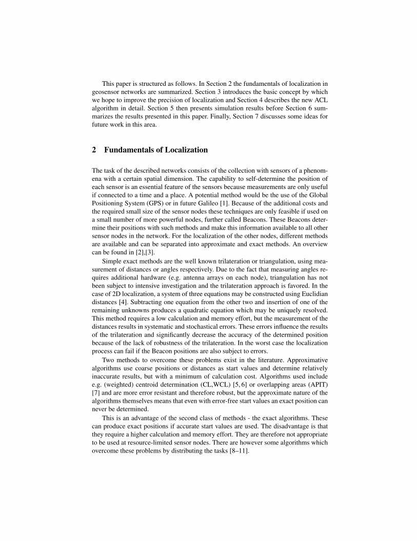
In the first simulation, 10 Beacons and 20 sensor nodes are distributed in the field. Threesensor intervals with range 49 and a distance error of σd = 1.0 are used. In the case thatall three sensor intervals do not overlap, their area represents ca. 36% of the total area.In a simulation with 10 Beacons there are 120 possible trilaterations. At this point, onlythe mean improvement V = E − EACL is considered. The data are sorted based onthe proportion of outliers, i.e. it is calculated how many of the 120 possible positionslie outside the correct sensor interval.

For each of the 20 nodes used there is a particular percentage of outliers and there-fore a line in the diagram (figure 4). Each line represents the absolute value of the mean

Implementierung des Modells in J-Sim ¯¯¯¯¯¯¯¯¯¯¯¯¯¯¯¯¯¯¯¯¯¯¯¯¯¯¯¯¯¯¯¯¯¯¯¯¯¯¯¯¯¯¯¯¯¯¯¯¯¯¯¯¯¯¯¯¯¯¯¯¯¯¯¯

28

Die Beacons senden zu Simulationsbeginn ein Paket mit ihrer Identifikation und

ihrer Position in das Netzwerk, welches von allen Knoten in Reichweite empfangen

wird. Gleichzeitig wird die Messung der Distanz zum jeweiligen Beacon durch

euklidische Entfernungsberechnung und Überlagerung mit einem zufälligen

gaußverteilten Fehler simuliert. (siehe Abschnitt 4.2) Jeder Knoten führt eine Liste

mit Beaconpositionen und seiner jeweiligen Entfernung zu diesen Beacons. Sobald

ein Knoten keine weiteren Beacons mehr empfängt, beginnt er mit der

Lokalisierung. Diese erfolgt unter Anwendung des in Abschnitt 4.3 beschriebenen

Modells und liefert die Simulationsergebnisse, welche im nächsten Kapitel näher

erläutert werden.

Abb. 13: Graphische Ausgabe eines Sensorfeldes mit 3 Sensorintervallen, 10 Beacons und 20 Knoten

Gleichzeitig werden die

graphische Ausgabe des

Sensorfeldes und der

Fehlerdiagramme

erzeugt. Zur späteren

Auswertung werden

diese Daten in externen

Dateien abgespeichert.

Nebenstehend in Abb. 13

ist eine solche graphische

Ausgabe dargestellt. Die

Sensorintervalle sind

grau unterlegt und die

einfachen Knoten zeigen

mit Linien zum Ort ihrer

Lokalisierung.

Das angezeigte Raster entspricht einer Einteilung in 10 m Abschnitte, sodass sich

ein 100 m x 100 m Feld ergibt, auf dem 10 Beacons und 20 einfache Sensoren

zufällig verteilt sind. Die Distanzabweichung in diesem Beispiel beträgt σd = 1.0.

Die drei dargestellten Sensorintervalle haben eine jeweilige Größe von 49

Rasterquadraten á 25 m², wobei das interne Raster auf 5 m x 5 m eingestellt ist.

Fig. 3. Screenshot of simulation results in J-Sim; triangles are Beacons and points with lines aresensor nodes with its error-vector; three darker areas represent sensor intervals

improvement which each node achieves with 120 trilaterations and the given number ofoutliers. In the case that multiple nodes have the same number of outliers a mean valueis calculated.

Since the raw data show a high scattering, a linear regression is used to emphasizethe trend. The improvement increases with an increasing number of outliers. This trendis not demonstratably linear, but a similar trend is observed over many simulations,leading to the assumption that the improvement is at least linear or even exponential.Similarly it can be seen that with a low number of outliers, up to ca. 15%, there is anegative improvement (i.e. a worsening). This shows that there is a certain minimumnumber of outliers under which the use of the ACL algorithm is not appropriate. Thislimit is dependent on the particular configuration and can not therefore be generallyspecified.

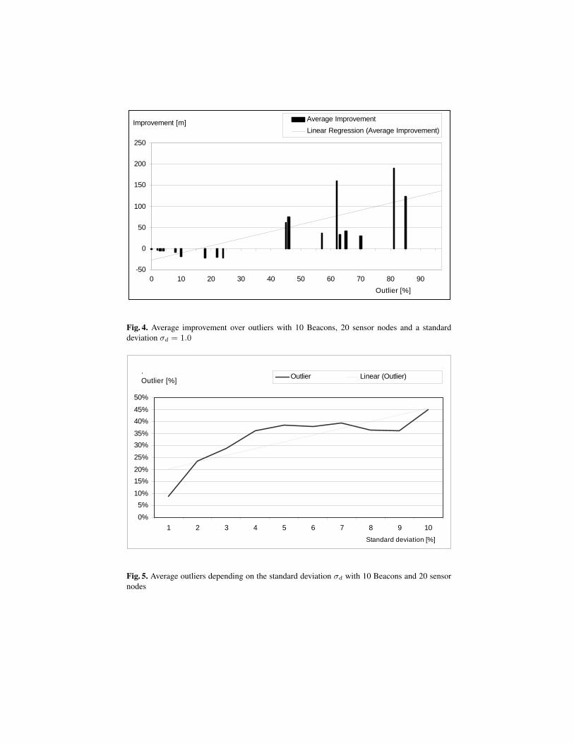
5.2 Correlation Between Number of Outliers and Distance Errors

The number of outliers is dependent on the error in the distance measurement, in thiscase the standard deviation σd. In the following simulation the same configuration as inSection 5.1 is used with different distance errors. The parameter σd is varied between1.0 and 10.0 with an interval of 1.0. The number of outliers is calculated as a functionof this parameter.

Optimierung des ACL-Algorithmus ¯¯¯¯¯¯¯¯¯¯¯¯¯¯¯¯¯¯¯¯¯¯¯¯¯¯¯¯¯¯¯¯¯¯¯¯¯¯¯¯¯¯¯¯¯¯¯¯¯¯¯¯¯¯¯¯¯¯¯¯¯¯¯¯

31

6.3 Auswertung der Simulationsergebnisse

Es folgen nun die Ergebnisse der Simulationen, deren Auswertung und die

Interpretation. Um den ACL-Algorithmus bewerten zu können, ist jeweils die

Verbesserung gegenüber dem gleichen Szenario ohne ACL untersucht worden.

6.3.1 Mittlere Verbesserung bei 10 Beacons

In dieser ersten Simulation wurden auf dem Feld 10 Beacons und 20 Sensorknoten

verteilt. Es wurde hier mit drei Sensorintervallen der Größe 49 und einem

Distanzfehler mit σd = 1.0 gerechnet. Für den Fall, dass alle drei Sensorintervalle

sich nicht überschneiden, entspricht deren Fläche etwa 36 % der Gesamtfläche. In

einer Simulation mit 10 Beacons gibt es ( ) 120103 = mögliche Trilaterationen. Es

wurde zunächst allein die mittlere Verbesserung V̄ untersucht. Die Daten sind nach

dem Anteil der Ausreißer sortiert, das heißt es wurde berechnet, wie viele der 120

möglichen Positionen außerhalb des korrekten Sensorintervalls lagen.

-50

0

50

100

150

200

250

0 10 20 30 40 50 60 70 80 90Outlier [%]

Improvement [m] Average ImprovementLinear Regression (Average Improvement)

Abb. 14: Durchschnittliche Verbesserung über dem Anteil an Ausreißern bei 10 Beacons, 20 Knoten und einer Standardabweichung σd = 1.0

Für jeden der verwendeten 20 Knoten ergibt sich ein bestimmter Prozentsatz an

Ausreißern und damit eine Linie im Diagramm. (siehe Abb. 14) Jede Linie

kennzeichnet den absoluten Wert der mittleren Verbesserung, die einer der Knoten

bei 120 Trilaterationen mit dem entsprechenden Anteil an Ausreißern erzielt hat.

Fig. 4. Average improvement over outliers with 10 Beacons, 20 sensor nodes and a standarddeviation σd = 1.0

Optimierung des ACL-Algorithmus ¯¯¯¯¯¯¯¯¯¯¯¯¯¯¯¯¯¯¯¯¯¯¯¯¯¯¯¯¯¯¯¯¯¯¯¯¯¯¯¯¯¯¯¯¯¯¯¯¯¯¯¯¯¯¯¯¯¯¯¯¯¯¯¯

32

Bei mehreren Knoten mit gleicher Anzahl an Ausreißern wurde die Verbesserung

gemittelt.

Da die reinen Daten sehr hohe Streuungen aufweisen, wurde eine lineare

Regressionsgerade eingefügt, welche den Trend verdeutlicht. Mit zunehmender

Anzahl von Ausreißern steigt die Verbesserung an. Dieser Trend ist nicht

nachweislich linear, jedoch wurde bei vielen Simulationen ein ähnliches Verhalten

beobachtet, sodass die Vermutung nahe liegt, dass die Verbesserung mindestens

linear oder sogar potentiell ansteigt. Gleichfalls zeigt sich bei geringem Anteil von

Ausreißern, bis etwa 15 %, dass die Verbesserung negativ ist. Das zeigt, dass eine

bestimmte untere Grenze für die Ausreißer existiert, unterhalb der die Anwendung

des ACL-Algorithmus nicht sinnvoll ist. Diese Grenze ist von der jeweiligen

Konfiguration abhängig und kann deshalb nicht allgemein angegeben werden.

6.3.2 Abhängigkeit der Anzahl der Ausreißer vom Distanzfehler

Der Anteil der Ausreißer ist wiederum vom Fehler bei der Distanzmessung, hier

also von der Standardabweichung σd abhängig. In den nächsten Simulationen

wurde die gleiche Konfiguration wie in Abschnitt 6.3.1 bei veränderlichen Distanz-

fehlern untersucht. Der Parameter σd wurde von 1.0 bis 10.0 in Einerschritten

eingestellt. Als Funktion davon wurde der Anteil der Ausreißer aufgenommen.

0%

5%10%

15%20%

25%

30%35%

40%45%

50%

1 2 3 4 5 6 7 8 9 10Standard deviation [%]

.Outlier [%] Outlier Linear (Outlier)

Abb. 15: Mittlerer Anteil der Ausreißer in Abhängigkeit von der Standardabweichung σd für 10 Beacons und 20 Knoten Fig. 5. Average outliers depending on the standard deviation σd with 10 Beacons and 20 sensor

nodes

Figure 5 shows the mean number of outliers in relation to σd over multiple sim-ulations. It shows that the number of outliers increases with an increasing standarddeviation. Again a trend line is shown to illustrate the trend. This emphasizes that thevalues have a high random component and deliver different results in each simulation.It is however clear that the mean proportion of 15% outliers is rapidly exceeded, whichindicates that the ACL algorithm will only be ineffective, or detrimental as in figure 4,where there is a very small σd.

5.3 Influence of the Size and Number of Sensor Intervals

Further important factors in the effectiveness of ACL are the size, number and positionof the sensor intervals. For the simulations, the intervals were individually parameter-ized by size and number, but randomly positioned. Alongside the random distributionof the sensors, this is one of the main reasons for the high variability of the resultingdata. There is therefore no explicit results from which a formula for the accuracy ofthe ACL in relation to these parameters can be derived. An investigation of the influ-ence of size and number of sensor intervals however resulted in the expected results. Anincreasing number of sensor intervals results in an increasing fragmentation of the mea-surement field into smaller sections with different sensor profiles. This is particularlythe case where the sensor intervals are larger and therefore overlap more. The numberof outliers thus increases with an increasing size and number of sensor intervals, whichresults in a greater improvement. It is also important to note that sensors which lie nearto an interval boundary profit most from the outlier detection because the probability ofan outlier is higher in these locations than in a homogenous region.Optimierung des ACL-Algorithmus

¯¯¯¯¯¯¯¯¯¯¯¯¯¯¯¯¯¯¯¯¯¯¯¯¯¯¯¯¯¯¯¯¯¯¯¯¯¯¯¯¯¯¯¯¯¯¯¯¯¯¯¯¯¯¯¯¯¯¯¯¯¯¯¯

34

0

5

10

15

20

25

30

3 6 9Number of sensor intervals

Outlier [%] Average Improvement [m]

Abb. 16: Anteil der Ausreißer und mittlere Verbesserung in Abhängigkeit von der Anzahl der Sensorintervalle bei 10 Beacons und 20 Knoten

In Abb. 16 ist diese Abhängigkeit dargestellt. Mit dem Anteil der Ausreißer steigt

auch die mittlere Verbesserung V̄ bei zunehmender Anzahl von Sensorintervallen.

Es wurde dazu ein Sensorintervall mit drei Teilflächen der jeweiligen Größe 49

erzeugt. Im zweiten Schritt wurde ein weiteres gleichartiges Sensorintervall

hinzugenommen und dann ein drittes, während die vorherigen jeweils in

konstanter Anordnung gehalten wurden. Des Weiteren wurden 10 Beacons,

20 Knoten und σd = 1.0 verwendet, was bedeutet, dass bei höheren Distanzfehlern

beide Kurven einen größeren Anstieg aufweisen würden.

6.3.4 Vergleich von mittlerer Verbesserung und Erstverbesserung

Aufgrund der verschiedenen Möglichkeiten eine endgültige Schätzposition zu

bestimmen wurden Versuche durchgeführt um die eine oder andere Möglichkeit zu

begünstigen. Dazu wurde auf einem Feld mit drei Sensorintervallen der Größe 49

mit 10 Beacons und 20 Knoten ein Vergleich der mittleren Verbesserung V̄ mit der

Erstverbesserung Vf durchgeführt. Die Werte wurden dabei jeweils über die

20 Knoten gemittelt, damit die Streuung nicht zu stark ins Gewicht fällt. Die

Standardabweichung der Distanzen wurde dazu wieder von 1.0 bis 10.0

durchlaufen.

Fig. 6. Outlier and average improvement depending on the number of sensor intervals with 10Beacons and 20 sensor nodes

Figure 6 shows this relationship. With an increasing number of outliers, the meanimprovement V also increases with an increasing number of sensor intervals. For this

case a sensor interval with three sub-regions of size 49 was created. In a second stepa further similar sensor interval was introduced and subsequently a third, whereby theprevious intervals were retained with a constant configuration. Furthermore, 10 Bea-cons, 20 nodes and σd = 1.0 were used, which indicates that with increasing distanceerrors both curves would show an increased slope.

5.4 Comparison of Mean Improvement and First Improvement

Due to the various possibilities for determining a final estimated position, experimentswere made which should favor each method. For this a field with three sensor intervalsof size 49 with 10 Beacons and 20 nodes was used to compare the mean improvementV with the first improvement Vf . The mean values from the 20 nodes were used toreduce the weight of the variation. The standard deviation of the distances was againvaried between 1.0 and 10.0. Optimierung des ACL-Algorithmus

¯¯¯¯¯¯¯¯¯¯¯¯¯¯¯¯¯¯¯¯¯¯¯¯¯¯¯¯¯¯¯¯¯¯¯¯¯¯¯¯¯¯¯¯¯¯¯¯¯¯¯¯¯¯¯¯¯¯¯¯¯¯¯¯

35

-5

0

5

10

15

20

25

30

35

1 2 3 4 5 6 7 8 9 10Standard deviation [%]

Improvement [m]

First ImprovementAverage ImprovementLinear (First Improvement)Linear (Average Improvement)

Abb. 17: Vergleich der mittleren Verbesserung und der Erstverbesserung in Abhängigkeit von der Standardabweichung σd

Es zeigt sich in Abb. 17 deutlich, dass die Erstverbesserung weit weniger stark

wächst als die mittlere Verbesserung. Das liegt zum einen daran, dass bei der

Erstverbesserung weit weniger Trilaterationen ausgewertet werden, zum anderen

aber auch daran, dass nur wenige Knoten überhaupt eine Erstverbesserung

aufweisen, weil sie nicht in der Nähe des Randes eines Intervalls liegen und damit

keine oder nur wenig Ausreißer besitzen. Auch diese Trends sind nicht unbedingt

linear und wurden durch Regressionsgeraden verdeutlicht.

Die mittlere Verbesserung erzielt hier erheblich bessere Ergebnisse und ist damit

die Methode der Wahl, jedoch müssen in Bezug auf die Praxistauglichkeit zwei

Punkte in Betracht gezogen werden:

1. Die Mittlere Verbesserung drückt eher aus, um wie viel der Algorithmus die

Lokalisierung verbessern könnte und ist deshalb nicht als absolut zu betrachten

2. Die Ersparung an Berechnung bei der Erstverbesserung

Wenn es darum geht eine möglichst genaue Lokalisierung vorzunehmen, so ist die

Mittelwertbildung die geeignete Methode, da sie alle zur Verfügung stehenden

Daten nutzt und ein sehr gutes Ergebnis liefern kann, gerade wenn die Ausreißer

tatsächlich natürlichen Ursprungs sind und damit keine gaußsche Streuung um die

exakte Position aufweisen.

Fig. 7. Comparison of the average improvement and the first improvement depending on thestandard deviation σd.

It is clear from figure 7 that the first improvement demonstrates a significantly lowerincrease in precision in comparison with the mean improvement. This is partly dueto the fact that significantly fewer trilaterations are considered, but also because onlya few nodes show any first improvement because they are not near the boundary ofan interval and therefore have few or no outliers. The trends are also in this case notnecessarily linear and are emphasized using regression lines. The mean improvement is

demonstrated here to deliver significantly better results and is therefore the method ofchoice, although the increased computational expense must also be considered.

6 Conclusion

This paper presented a new approach to improve the precision of localization algorithmsin sensor networks which were previously too inexact or calculation-intensive for use.The spatial correlation of the measured sensor values is used for this. The principle usedis that sensor observations vary within defined boundaries depending on their location.We have presented a way to use this information by defining sensor intervals. These maybe used after localization by trilateration to test the reliability of the resulting estimatedpositions by comparing the observed values with the sensor intervals. This method waspresented as the ACL algorithm together with investigations as to its effectiveness.

Simulations showed that the use of the ACL algorithm can improve the mean errorof the localization using trilateration by up to 30% when the measured distances have astandard deviation of 10%. With a 5% standard deviation the improvement is ca. 12%.These results were obtained using three known sensor intervals, which coverered aroundone third of the measurement field. With further prerequisites the localization couldbe further improved. Only with very small distance errors with a standard deviationof under 1% is the use of the algorithm not appropriate as in this range an increasedlocalization error was determined.

In conclusion, it has been shown that using the sensor measurement data for lo-calization is a sensible approach, particularly as these data are already available. Asignificant improvement is possible with minimal additional complexity of calculationon the sensor nodes. The concrete use is however very dependent on how accurate theavailable measurements are and how many prerequisites can be determined. An advan-tage of this method is that no additional errors are produced since it effectively involvesno more than a filtering of the input values. This can have negative consequences inisolated cases, but from an overall standpoint leads to a more precise result. A furtheradvantage of the model presented here is the possibility to formulate arbitrarily complexprerequisites.

The ACL algorithm can be considered as an efficient additional method for local-ization. Even with relatively few preconditions it is possible to improve the localizationor to verify the positions. In particular in combination with approximate algorithms itis possible to obtain good results, but also with exact positioning where large distanceerrors are present then the ACL is of benefit.

7 Future Work

The idea presented here is by no means optimally applied. It is necessary to find a bet-ter mathematical model on which the ACL algorithm may operate. Currently a simplecomparison of measured values with sensor values is made. This is computationallyeasy, but the spatial information can only be very coarsely exploited. A model such asconvex optimization should be considered instead.

Furthermore, the definition of sensor intervals is still very static and inflexible. Thiscould also lead to problems at run-time as the sensor intervals may vary over time.To continue the example of light intensity sensors, the intervals may vary strongly be-tween day and night or summer and winter. To solve this problem an automatic intervalgeneration may be used, which may be possible with e.g. an evolutionary algorithm orsimmulated annealing.

Ultimately the additional information are used purely as a means of detecting out-liers in the trilateration. The aim is to combine further localization algorithms withthis information to obtain an increased precision and to possibly weight the defectivedistance measurements and error prone sensor data. It is conceivable that the brieflyintroduced WCL algorithm may be thus made more precise. This is however primarilyreliant on the effectiveness of new mathematical models.

Acknowledgment

This work was supported by the German Research Foundation under grant numberTI254/15-1 and BI467/17-1 (keyword: Geosens). Thanks also to the reviewers whotook the time to provide constructive criticism which has helped improve this paper.

References

1. Gibson, J.: The Mobile Communications Handbook. CRC Press (1996)2. Reichenbach, F.: Resource-aware Algorithms for exact Localization in Wireless Sensor Net-

works. PhD thesis, University of Rostock (2007)3. Stefanidis, A., Nittel, S.: GeoSensor Networks. CRC Press (2004)4. Bulusu, N., Heidemann, J., Estrin, D.: Adaptive beacon placement. 21st International Con-

ference on Distributed Computing Systems (2001) 489–4985. Bulusu, N.: Gps-less low cost outdoor localization for very small devices. IEEE Personal

Communications Magazine 7 (2000) 28–346. Blumenthal, J., Reichenbach, F., Timmermann, D.: Precise positioning with a low complex-

ity algorithm in ad hoc wireless sensor networks. PIK - Praxis der Informationsverarbeitungund Kommunikation 28 (2005) 80–85

7. He, T., Huang, C., Blum, B., Stankovic, J., Abdelzaher, T.: Range-free localization schemesfor large scale sensor networks. 9th Annual International Conference on Mobile Computingand Networking (2003) 81–95 San Diego, CA, USA.

8. Reichenbach, F., Born, A., Timmermann, D., Bill, R.: Splitting the linear least squares prob-lem for precise localization in geosensor networks. Proceedings of the 4th InternationalConference on GIScience (2006) 321–337 Muenster, Germany.

9. Reichenbach, F., Born, A., Timmermann, D., Bill, R.: A distributed linear least squaresmethod for precise localization with low complexity in wireless sensor networks. 2nd IEEEInternational Conference on Distributed Computing in Sensor Systems (2006) 514–528 SanFrancisco, USA.

10. Savvides, A., Han, C.C., Srivastava, M.: Dynamic fine grained localization in ad-hoc net-works of sensors. 7th ACM MobiCom (2001) 166–179 Rome, Italy.

11. Doherty, L., Pister, K., Ghaoui, L.: Convex position estimation in wireless sensor networks.20th Annual Joint Conference of the IEEE Computer and Communications (2001) 1655–1663 Anchorage, AK, USA.

12. Vellidis, G., Garrick, V., Pocknee, S., Perry, C., Kvien, C., Tucker, M.: How wireless willchange agriculture. Stafford, J.V. Precision Agriculture ’07 (2007) 57–67

13. Konstantinos, K., Panagiotis, K., Apostolos, X., George, S.: Proposing a method of networktopology optimization in wireless sensor in precision agriculture. Proceedings of the 6thEuropean Conference on Precision Agriculture (2007)

14. : J-sim: A component-based, compositional simulation environment, http://www.j-sim.org/(2007)

15. Strehlow, C.: Genauigkeitserhoehung der Lokalisierung in drahtlosen Sensornetzwerkendurch Einbeziehung von Sensormessdaten (2007) Seminar Paper.