Improving neural networks by preventingco-adaptation of feature detectors

G. E. Hinton∗, N. Srivastava, A. Krizhevsky, I. Sutskever and R. R. SalakhutdinovDepartment of Computer Science, University of Toronto,6 King’s College Rd, Toronto, Ontario M5S 3G4, Canada

∗To whom correspondence should be addressed; E-mail: hinton@cs.toronto.edu

When a large feedforward neural network is trained on a small training set,it typically performs poorly on held-out test data. This “overfitting” is greatlyreduced by randomly omitting half of the feature detectors on each trainingcase. This prevents complex co-adaptations in which a feature detector is onlyhelpful in the context of several other specific feature detectors. Instead, eachneuron learns to detect a feature that is generally helpful for producing thecorrect answer given the combinatorially large variety of internal contexts inwhich it must operate. Random “dropout” gives big improvements on manybenchmark tasks and sets new records for speech and object recognition.

A feedforward, artificial neural network uses layers of non-linear “hidden” units betweenits inputs and its outputs. By adapting the weights on the incoming connections of these hiddenunits it learns feature detectors that enable it to predict the correct output when given an inputvector (1). If the relationship between the input and the correct output is complicated and thenetwork has enough hidden units to model it accurately, there will typically be many differentsettings of the weights that can model the training set almost perfectly, especially if there isonly a limited amount of labeled training data. Each of these weight vectors will make differentpredictions on held-out test data and almost all of them will do worse on the test data than onthe training data because the feature detectors have been tuned to work well together on thetraining data but not on the test data.

Overfitting can be reduced by using “dropout” to prevent complex co-adaptations on thetraining data. On each presentation of each training case, each hidden unit is randomly omittedfrom the network with a probability of 0.5, so a hidden unit cannot rely on other hidden unitsbeing present. Another way to view the dropout procedure is as a very efficient way of perform-ing model averaging with neural networks. A good way to reduce the error on the test set is toaverage the predictions produced by a very large number of different networks. The standard

1

arX

iv:1

207.

0580

v1 [

cs.N

E]

3 J

ul 2

012

way to do this is to train many separate networks and then to apply each of these networks tothe test data, but this is computationally expensive during both training and testing. Randomdropout makes it possible to train a huge number of different networks in a reasonable time.There is almost certainly a different network for each presentation of each training case but allof these networks share the same weights for the hidden units that are present.

We use the standard, stochastic gradient descent procedure for training the dropout neuralnetworks on mini-batches of training cases, but we modify the penalty term that is normallyused to prevent the weights from growing too large. Instead of penalizing the squared length(L2 norm) of the whole weight vector, we set an upper bound on the L2 norm of the incomingweight vector for each individual hidden unit. If a weight-update violates this constraint, werenormalize the weights of the hidden unit by division. Using a constraint rather than a penaltyprevents weights from growing very large no matter how large the proposed weight-update is.This makes it possible to start with a very large learning rate which decays during learning,thus allowing a far more thorough search of the weight-space than methods that start with smallweights and use a small learning rate.

At test time, we use the “mean network” that contains all of the hidden units but with theiroutgoing weights halved to compensate for the fact that twice as many of them are active.In practice, this gives very similar performance to averaging over a large number of dropoutnetworks. In networks with a single hidden layer of N units and a “softmax” output layer forcomputing the probabilities of the class labels, using the mean network is exactly equivalentto taking the geometric mean of the probability distributions over labels predicted by all 2N

possible networks. Assuming the dropout networks do not all make identical predictions, theprediction of the mean network is guaranteed to assign a higher log probability to the correctanswer than the mean of the log probabilities assigned by the individual dropout networks (2).Similarly, for regression with linear output units, the squared error of the mean network isalways better than the average of the squared errors of the dropout networks.

We initially explored the effectiveness of dropout using MNIST, a widely used benchmarkfor machine learning algorithms. It contains 60,000 28x28 training images of individual handwritten digits and 10,000 test images. Performance on the test set can be greatly improved byenhancing the training data with transformed images (3) or by wiring knowledge about spatialtransformations into a convolutional neural network (4) or by using generative pre-training toextract useful features from the training images without using the labels (5). Without using anyof these tricks, the best published result for a standard feedforward neural network is 160 errorson the test set. This can be reduced to about 130 errors by using 50% dropout with separate L2constraints on the incoming weights of each hidden unit and further reduced to about 110 errorsby also dropping out a random 20% of the pixels (see figure 1).

Dropout can also be combined with generative pre-training, but in this case we use a smalllearning rate and no weight constraints to avoid losing the feature detectors discovered by thepre-training. The publically available, pre-trained deep belief net described in (5) got 118 errorswhen it was fine-tuned using standard back-propagation and 92 errors when fine-tuned using50% dropout of the hidden units. When the publically available code at URL was used to pre-

2

Fig. 1: The error rate on the MNIST test set for a variety of neural network architectures trainedwith backpropagation using 50% dropout for all hidden layers. The lower set of lines alsouse 20% dropout for the input layer. The best previously published result for this task usingbackpropagation without pre-training or weight-sharing or enhancements of the training set isshown as a horizontal line.

train a deep Boltzmann machine five times, the unrolled network got 103, 97, 94, 93 and 88errors when fine-tuned using standard backpropagation and 83, 79, 78, 78 and 77 errors whenusing 50% dropout of the hidden units. The mean of 79 errors is a record for methods that donot use prior knowledge or enhanced training sets (For details see Appendix A).

We then applied dropout to TIMIT, a widely used benchmark for recognition of clean speechwith a small vocabulary. Speech recognition systems use hidden Markov models (HMMs) todeal with temporal variability and they need an acoustic model that determines how well a frameof coefficients extracted from the acoustic input fits each possible state of each hidden Markovmodel. Recently, deep, pre-trained, feedforward neural networks that map a short sequence offrames into a probability distribution over HMM states have been shown to outperform tradionalGaussian mixture models on both TIMIT (6) and a variety of more realistic large vocabularytasks (7, 8).

Figure 2 shows the frame classification error rate on the core test set of the TIMIT bench-mark when the central frame of a window is classified as belonging to the HMM state that isgiven the highest probability by the neural net. The input to the net is 21 adjacent frames with anadvance of 10ms per frame. The neural net has 4 fully-connected hidden layers of 4000 units per

3

Fig. 2: The frame classification error rate on the core test set of the TIMIT benchmark. Com-parison of standard and dropout finetuning for different network architectures. Dropout of 50%of the hidden units and 20% of the input units improves classification.

layer and 185 “softmax” output units that are subsequently merged into the 39 distinct classesused for the benchmark. Dropout of 50% of the hidden units significantly improves classifica-tion for a variety of different network architectures (see figure 2). To get the frame recognitionrate, the class probabilities that the neural network outputs for each frame are given to a decoderwhich knows about transition probabilities between HMM states and runs the Viterbi algorithmto infer the single best sequence of HMM states. Without dropout, the recognition rate is 22.7%and with dropout this improves to 19.7%, which is a record for methods that do not use anyinformation about speaker identity.

CIFAR-10 is a benchmark task for object recognition. It uses 32x32 downsampled colorimages of 10 different object classes that were found by searching the web for the names of theclass (e.g. dog) or its subclasses (e.g. Golden Retriever). These images were labeled by handto produce 50,000 training images and 10,000 test images in which there is a single dominantobject that could plausibly be given the class name (9) (see figure 3). The best published errorrate on the test set, without using transformed data, is 18.5% (10). We achieved an error rate of16.6% by using a neural network with three convolutional hidden layers interleaved with three“max-pooling” layers that report the maximum activity in local pools of convolutional units.These six layers were followed by one locally-connected layer (For details see Appendix D) .Using dropout in the last hidden layer gives an error rate of 15.6%.

ImageNet is an extremely challenging object recognition dataset consisting of thousands ofhigh-resolution images of thousands of classes of object (11). In 2010, a subset of 1000 classeswith roughly 1000 examples per class was the basis of an object recognition competition in

4

Fig. 3: Ten examples of the class “bird” from the CIFAR-10 test set illustrating the varietyof types of bird, viewpoint, lighting and background. The neural net gets all but the last twoexamples correct.

which the winning entry, which was actually an average of six separate models, achieved anerror rate of 47.2% on the test set. The current state-of-the-art result on this dataset is 45.7%(12). We achieved comparable performance of 48.6% error using a single neural network withfive convolutional hidden layers interleaved with “max-pooling” layer followed by two globallyconnected layers and a final 1000-way softmax layer. All layers had L2 weight constraints onthe incoming weights of each hidden unit. Using 50% dropout in the sixth hidden layer reducesthis to a record 42.4% (For details see Appendix E).

For the speech recognition dataset and both of the object recognition datasets it is necessaryto make a large number of decisions in designing the architecture of the net. We made thesedecisions by holding out a separate validation set that was used to evaluate the performance ofa large number of different architectures and we then used the architecture that performed bestwith dropout on the validation set to assess the performance of dropout on the real test set.

The Reuters dataset contains documents that have been labeled with a hierarchy of classes.We created training and test sets each containing 201,369 documents from 50 mutually exclu-sive classes. Each document was represented by a vector of counts for 2000 common non-stopwords, with each count C being transformed to log(1 +C). A feedforward neural network with2 fully connected layers of 2000 hidden units trained with backpropagation gets 31.05% erroron the test set. This is reduced to 29.62% by using 50% dropout (Appendix C).

We have tried various dropout probabilities and almost all of them improve the generaliza-tion performance of the network. For fully connected layers, dropout in all hidden layers worksbetter than dropout in only one hidden layer and more extreme probabilities tend to be worse,which is why we have used 0.5 throughout this paper. For the inputs, dropout can also help,

Fig. 4: Some Imagenet test cases with the probabilities of the best 5 labels underneath. Manyof the top 5 labels are quite plausible.

5

though it it often better to retain more than 50% of the inputs. It is also possible to adapt theindividual dropout probability of each hidden or input unit by comparing the average perfor-mance on a validation set with the average performance when the unit is present. This makesthe method work slightly better. For datasets in which the required input-output mapping has anumber of fairly different regimes, performance can probably be further improved by makingthe dropout probabilities be a learned function of the input, thus creating a statistically efficient“mixture of experts” (13) in which there are combinatorially many experts, but each parametergets adapted on a large fraction of the training data.

Dropout is considerably simpler to implement than Bayesian model averaging which weightseach model by its posterior probability given the training data. For complicated model classes,like feedforward neural networks, Bayesian methods typically use a Markov chain Monte Carlomethod to sample models from the posterior distribution (14). By contrast, dropout with aprobability of 0.5 assumes that all the models will eventually be given equal importance in thecombination but the learning of the shared weights takes this into account. At test time, the factthat the dropout decisions are independent for each unit makes it very easy to approximate thecombined opinions of exponentially many dropout nets by using a single pass through the meannet. This is far more efficient than averaging the predictions of many separate models.

A popular alternative to Bayesian model averaging is “bagging” in which different modelsare trained on different random selections of cases from the training set and all models are givenequal weight in the combination (15). Bagging is most often used with models such as decisiontrees because these are very quick to fit to data and very quick at test time (16). Dropout allowsa similar approach to be applied to feedforward neural networks which are much more powerfulmodels. Dropout can be seen as an extreme form of bagging in which each model is trained ona single case and each parameter of the model is very strongly regularized by sharing it withthe corresponding parameter in all the other models. This is a much better regularizer than thestandard method of shrinking parameters towards zero.

A familiar and extreme case of dropout is “naive bayes” in which each input feature istrained separately to predict the class label and then the predictive distributions of all the featuresare multiplied together at test time. When there is very little training data, this often works muchbetter than logistic classification which trains each input feature to work well in the context ofall the other features.

Finally, there is an intriguing similarity between dropout and a recent theory of the role ofsex in evolution (17). One possible interpretation of the theory of mixability articulated in (17)is that sex breaks up sets of co-adapted genes and this means that achieving a function by usinga large set of co-adapted genes is not nearly as robust as achieving the same function, perhapsless than optimally, in multiple alternative ways, each of which only uses a small number ofco-adapted genes. This allows evolution to avoid dead-ends in which improvements in fitnessrequire co- ordinated changes to a large number of co-adapted genes. It also reduces the proba-bility that small changes in the environment will cause large decreases in fitness a phenomenonwhich is known as “overfitting” in the field of machine learning.

6

References and Notes1. D. E. Rumelhart, G. E. Hinton, R. J. Williams, Nature 323, 533 (1986).

2. G. E. Hinton, Neural Computation 14, 1771 (2002).

3. L. M. G. D. C. Ciresan, U. Meier, J. Schmidhuber, Neural Computation 22, 3207 (2010).

4. Y. B. Y. Lecun, L. Bottou, P. Haffner, Proceedings of the IEEE 86, 2278 (1998).

5. G. E. Hinton, R. Salakhutdinov, Science 313, 504 (2006).

6. A. Mohamed, G. Dahl, G. Hinton, IEEE Transactions on Audio, Speech, and LanguageProcessing, 20, 14 (2012).

7. G. Dahl, D. Yu, L. Deng, A. Acero, IEEE Transactions on Audio, Speech, and LanguageProcessing, 20, 30 (2012).

8. N. Jaitly, P. Nguyen, A. Senior, V. Vanhoucke, An Application OF Pretrained Deep Neu-ral Networks To Large Vocabulary Conversational Speech Recognition, Tech. Rep. 001,Department of Computer Science, University of Toronto (2012).

9. A. Krizhevsky, Learning multiple layers of features from tiny images, Tech. Rep. 001, De-partment of Computer Science, University of Toronto (2009).

10. A. Coates, A. Y. Ng, ICML (2011), pp. 921–928.

11. J. Deng, et al., CVPR09 (2009).

12. J. Sanchez, F. Perronnin, CVPR11 (2011).

13. S. J. N. R. A. Jacobs, M. I. Jordan, G. E. Hinton, Neural Computation 3, 79 (1991).

14. R. M. Neal, Bayesian Learning for Neural Networks, Lecture Notes in Statistics No. 118(Springer-Verlag, New York, 1996).

15. L. Breiman, Machine Learning 24, 123 (1996).

16. L. Breiman, Machine Learning 45, 5 (2001).

17. J. D. A. Livnat, C. Papadimitriou, M. W. Feldman, PNAS 105, 19803 (2008).

18. R. R. Salakhutdinov, G. E. Hinton, Artificial Intelligence and Statistics (2009).

19. D. D. Lewis, T. G. R. Y. Yang, Journal of Machine Learning 5, 361 (2004).

20. We thank N. Jaitly for help with TIMIT, H. Larochelle, R. Neal, K. Swersky and C.K.I.Williams for helpful discussions, and NSERC, Google and Microsoft Research for funding.GEH and RRS are members of the Canadian Institute for Advanced Research.

7

A Experiments on MNIST

A.1 Details for dropout trainingThe MNIST dataset consists of 28× 28 digit images - 60,000 for training and 10,000 for testing.The objective is to classify the digit images into their correct digit class. We experimented withneural nets of different architectures (different number of hidden units and layers) to evaluatethe sensitivity of the dropout method to these choices. We show results for 4 nets (784-800-800-10, 784-1200-1200-10, 784-2000-2000-10, 784-1200-1200-1200-10). For each of thesearchitectures we use the same dropout rates - 50% dropout for all hidden units and 20% dropoutfor visible units. We use stochastic gradient descent with 100-sized minibatches and a cross-entropy objective function. An exponentially decaying learning rate is used that starts at thevalue of 10.0 (applied to the average gradient in each minibatch). The learning rate is multipliedby 0.998 after each epoch of training. The incoming weight vector corresponding to each hiddenunit is constrained to have a maximum squared length of l. If, as a result of an update, thesquared length exceeds l, the vector is scaled down so as to make it have a squared lengthof l. Using cross validation we found that l = 15 gave best results. Weights are initialzedto small random values drawn from a zero-mean normal distribution with standard deviation0.01. Momentum is used to speed up learning. The momentum starts off at a value of 0.5 andis increased linearly to 0.99 over the first 500 epochs, after which it stays at 0.99. Also, thelearning rate is multiplied by a factor of (1-momentum). No weight decay is used. Weightswere updated at the end of each minibatch. Training was done for 3000 epochs. The weightupdate takes the following form:

∆wt = pt∆wt−1 − (1− pt)εt〈∇wL〉wt = wt−1 + ∆wt,

where,

εt = ε0ft

pt =

{tTpi + (1− t

T)pf t < T

pf t ≥ T

with ε0 = 10.0, f = 0.998, pi = 0.5, pf = 0.99, T = 500. While using a constant learningrate also gives improvements over standard backpropagation, starting with a high learning rateand decaying it provided a significant boost in performance. Constraining input vectors tohave a fixed length prevents weights from increasing arbitrarily in magnitude irrespective of thelearning rate. This gives the network a lot of opportunity to search for a good configuration inthe weight space. As the learning rate decays, the algorithm is able to take smaller steps andfinds the right step size at which it can make learning progress. Using a high final momentumdistributes gradient information over a large number of updates making learning stable in thisscenario where each gradient computation is for a different stochastic network.

8

A.2 Details for dropout finetuningApart from training a neural network starting from random weights, dropout can also be usedto finetune pretrained models. We found that finetuning a model using dropout with a smalllearning rate can give much better performace than standard backpropagation finetuning.

Deep Belief Nets - We took a neural network pretrained using a Deep Belief Network (5).It had a 784-500-500-2000 architecture and was trained using greedy layer-wise ContrastiveDivergence learning 1. Instead of fine-tuning it with the usual backpropagation algorithm, weused the dropout version of it. Dropout rate was same as before : 50% for hidden units and 20%for visible units. A constant small learning rate of 1.0 was used. No constraint was imposed onthe length of incoming weight vectors. No weight decay was used. All other hyper-parameterswere set to be the same as before. The model was trained for 1000 epochs with stochstic gradientdescent using minibatches of size 100. While standard back propagation gave about 118 errors,dropout decreased the errors to about 92.

Deep Boltzmann Machines - We also took a pretrained Deep Boltzmann Machine (18) 2

(784-500-1000-10) and finetuned it using dropout-backpropagation. The model uses a 1784 -500 - 1000 - 10 architecture (The extra 1000 input units come from the mean-field activationsof the second layer of hidden units in the DBM, See (18) for details). All finetuning hyper-parameters were set to be the same as the ones used for a Deep Belief Network. We were ableto get a mean of about 79 errors with dropout whereas usual finetuning gives about 94 errors.

A.3 Effect on featuresOne reason why dropout gives major improvements over backpropagation is that it encourageseach individual hidden unit to learn a useful feature without relying on specific other hiddenunits to correct its mistakes. In order to verify this and better understand the effect of dropout onfeature learning, we look at the first level of features learned by a 784-500-500 neural networkwithout any generative pre-training. The features are shown in Figure 5. Each panel shows 100random features learned by each network. The features that dropout learns are simpler and looklike strokes, whereas the ones learned by standard backpropagation are difficult to interpret.This confirms that dropout indeed forces the discriminative model to learn good features whichare less co-adapted and leads to better generalization.

B Experiments on TIMITThe TIMIT Acoustic-Phonetic Continuous Speech Corpus is a standard dataset used for eval-uation of automatic speech recognition systems. It consists of recordings of 630 speakers of 8dialects of American English each reading 10 phonetically-rich sentences. It also comes with

1For code see http://www.cs.toronto.edu/˜hinton/MatlabForSciencePaper.html2 For code see http://www.utstat.toronto.edu/˜rsalakhu/DBM.html

9

(a) (b)

Fig. 5: Visualization of features learned by first layer hidden units for (a) backprop and (b)dropout on the MNIST dataset.

the word and phone-level transcriptions of the speech. The objective is to convert a given speechsignal into a transcription sequence of phones. This data needs to be pre-processed to extractinput features and output targets. We used Kaldi, an open source code library for speech 3, topre-process the dataset so that our results can be reproduced exactly. The inputs to our networksare log filter bank responses. They are extracted for 25 ms speech windows with strides of 10ms.

Each dimension of the input representation was normalized to have mean 0 and variance 1.Minibatches of size 100 were used for both pretraining and dropout finetuning. We tried severalnetwork architectures by varying the number of input frames (15 and 31), number of layers inthe neural network (3, 4 and 5) and the number of hidden units in each layer (2000 and 4000).Figure 6 shows the validation error curves for a number of these combinations. Using dropoutconsistently leads to lower error rates.

B.1 PretrainingFor all our experiments on TIMIT, we pretrain the neural network with a Deep Belief Net-work (5). Since the inputs are real-valued, the first layer was pre-trained as a Gaussian RBM.

3http://kaldi.sourceforge.net

10

(a)

(b)

Fig. 6: Frame classification error and cross-entropy on the (a) Training and (b) Validation setas learning progresses. The training error is computed using the stochastic nets.

11

Visible biases were initialized to zero and weights to random numbers sampled from a zero-mean normal distribution with standard deviation 0.01. The variance of each visible unit wasset to 1.0 and not learned. Learning was done by minimizing Contrastive Divergence. Momen-tum was used to speed up learning. Momentum started at 0.5 and was increased linearly to 0.9over 20 epochs. A learning rate of 0.001 on the average gradient was used (which was thenmultiplied by 1-momentum). An L2 weight decay of 0.001 was used. The model was trainedfor 100 epochs.

All subsequent layers were trained as binary RBMs. A learning rate of 0.01 was used. Thevisible bias of each unit was initialized to log(p/(1 − p)) where p was the mean activation ofthat unit in the dataset. All other hyper-parameters were set to be the same as those we used forthe Gaussian RBM. Each layer was trained for 50 epochs.

B.2 Dropout FinetuningThe pretrained RBMs were used to initialize the weights in a neural network. The networkwas then finetuned with dropout-backpropagation. Momentum was increased from 0.5 to 0.9linearly over 10 epochs. A small constant learning rate of 1.0 was used (applied to the averagegradient on a minibatch). All other hyperparameters are the same as for MNIST dropout fine-tuning. The model needs to be run for about 200 epochs to converge. The same network wasalso finetuned with standard backpropagation using a smaller learning rate of 0.1, keeping allother hyperparameters

Figure 6 shows the frame classification error and cross-entropy objective value on the train-ing and validation sets. We compare the performance of dropout and standard backpropaga-tion on several network architectures and input representations. Dropout consistently achieveslower error and cross-entropy. It significantly controls overfitting, making the method robustto choices of network architecture. It allows much larger nets to be trained and removes theneed for early stopping. We also observed that the final error obtained by the model is not verysensitive to the choice of learning rate and momentum.

C Experiments on ReutersReuters Corpus Volume I (RCV1-v2) (19) is an archive of 804,414 newswire stories that havebeen manually categorized into 103 topics4. The corpus covers four major groups: corpo-rate/industrial, economics, government/social, and markets. Sample topics include Energy Mar-kets, Accounts/Earnings, Government Borrowings, Disasters and Accidents, Interbank Markets,Legal/Judicial, Production/Services, etc. The topic classes form a tree which is typically ofdepth three.

We took the dataset and split it into 63 classes based on the the 63 categories at the second-level of the category tree. We removed 11 categories that did not have any data and one category

4The corpus is available at http://www.ai.mit.edu/projects/jmlr/papers/volume5/lewis04a/lyrl2004 rcv1v2 README.htm

12

that had only 4 training examples. We also removed one category that covered a huge chunk(25%) of the examples. This left us with 50 classes and 402,738 documents. We divided thedocuments into equal-sized training and test sets randomly. Each document was representedusing the 2000 most frequent non-stopwords in the dataset.

(a) (b)

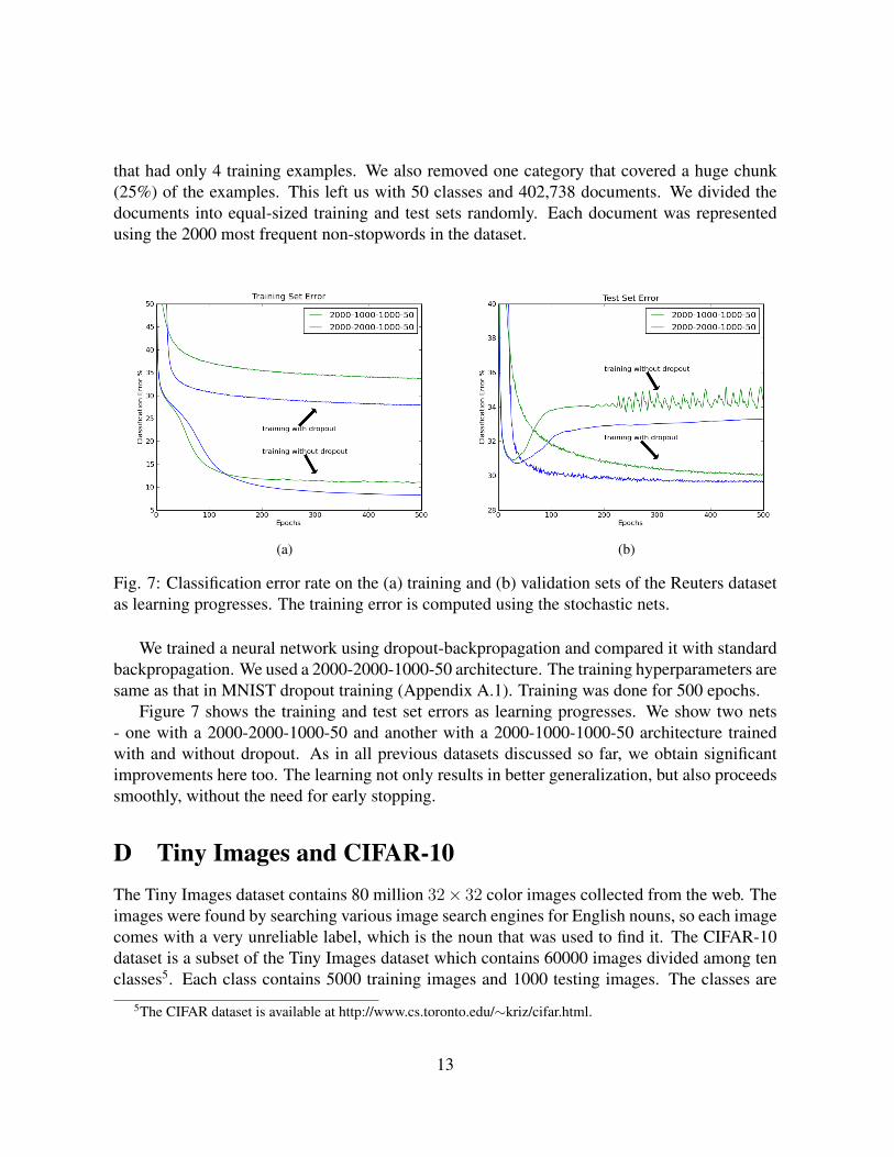
Fig. 7: Classification error rate on the (a) training and (b) validation sets of the Reuters datasetas learning progresses. The training error is computed using the stochastic nets.

We trained a neural network using dropout-backpropagation and compared it with standardbackpropagation. We used a 2000-2000-1000-50 architecture. The training hyperparameters aresame as that in MNIST dropout training (Appendix A.1). Training was done for 500 epochs.

Figure 7 shows the training and test set errors as learning progresses. We show two nets- one with a 2000-2000-1000-50 and another with a 2000-1000-1000-50 architecture trainedwith and without dropout. As in all previous datasets discussed so far, we obtain significantimprovements here too. The learning not only results in better generalization, but also proceedssmoothly, without the need for early stopping.

D Tiny Images and CIFAR-10The Tiny Images dataset contains 80 million 32× 32 color images collected from the web. Theimages were found by searching various image search engines for English nouns, so each imagecomes with a very unreliable label, which is the noun that was used to find it. The CIFAR-10dataset is a subset of the Tiny Images dataset which contains 60000 images divided among tenclasses5. Each class contains 5000 training images and 1000 testing images. The classes are

5The CIFAR dataset is available at http://www.cs.toronto.edu/∼kriz/cifar.html.

13

airplane, automobile, bird, cat, deer, dog, frog, horse, ship, and truck. The CIFAR-10 datasetwas obtained by filtering the Tiny Images dataset to remove images with incorrect labels. TheCIFAR-10 images are highly varied, and there is no canonical viewpoint or scale at whichthe objects appear. The only criteria for including an image were that the image contain onedominant instance of a CIFAR-10 class, and that the object in the image be easily identifiableas belonging to the class indicated by the image label.

E ImageNetImageNet is a dataset of millions of labeled images in thousands of categories. The imageswere collected from the web and labelled by human labellers using Amazon’s Mechanical Turkcrowd-sourcing tool. In 2010, a subset of roughly 1000 images in each of 1000 classes was thebasis of an object recognition competition, a part of the Pascal Visual Object Challenge. Thisis the version of ImageNet on which we performed our experiments. In all, there are roughly1.3 million training images, 50000 validation images, and 150000 testing images. This datasetis similar in spirit to the CIFAR-10, but on a much bigger scale. The images are full-resolution,and there are 1000 categories instead of ten. Another difference is that the ImageNet imagesoften contain multiple instances of ImageNet objects, simply due to the sheer number of objectclasses. For this reason, even a human would have difficulty approaching perfect accuracy onthis dataset. For our experiments we resized all images to 256× 256 pixels.

F Convolutional Neural NetworksOur models for CIFAR-10 and ImageNet are deep, feed-forward convolutional neural networks(CNNs). Feed-forward neural networks are models which consist of several layers of “neurons”,where each neuron in a given layer applies a linear filter to the outputs of the neurons in theprevious layer. Typically, a scalar bias is added to the filter output and a nonlinear activationfunction is applied to the result before the neuron’s output is passed to the next layer. The linearfilters and biases are referred to as weights, and these are the parameters of the network that arelearned from the training data.

CNNs differ from ordinary neural networks in several ways. First, neurons in a CNN areorganized topographically into a bank that reflects the organization of dimensions in the inputdata. So for images, the neurons are laid out on a 2D grid. Second, neurons in a CNN apply fil-ters which are local in extent and which are centered at the neuron’s location in the topographicorganization. This is reasonable for datasets where we expect the dependence of input dimen-sions to be a decreasing function of distance, which is the case for pixels in natural images.In particular, we expect that useful clues to the identity of the object in an input image can befound by examining small local neighborhoods of the image. Third, all neurons in a bank applythe same filter, but as just mentioned, they apply it at different locations in the input image. Thisis reasonable for datasets with roughly stationary statistics, such as natural images. We expect

14

that the same kinds of structures can appear at all positions in an input image, so it is reasonableto treat all positions equally by filtering them in the same way. In this way, a bank of neuronsin a CNN applies a convolution operation to its input. A single layer in a CNN typically hasmultiple banks of neurons, each performing a convolution with a different filter. These banks ofneurons become distinct input channels into the next layer. The distance, in pixels, between theboundaries of the receptive fields of neighboring neurons in a convolutional bank determinesthe stride with which the convolution operation is applied. Larger strides imply fewer neuronsper bank. Our models use a stride of one pixel unless otherwise noted.

One important consequence of this convolutional shared-filter architecture is a drastic re-duction in the number of parameters relative to a neural net in which all neurons apply differentfilters. This reduces the net’s representational capacity, but it also reduces its capacity to overfit,so dropout is far less advantageous in convolutional layers.

F.1 PoolingCNNs typically also feature “pooling” layers which summarize the activities of local patchesof neurons in convolutional layers. Essentially, a pooling layer takes as input the output of aconvolutional layer and subsamples it. A pooling layer consists of pooling units which are laidout topographically and connected to a local neighborhood of convolutional unit outputs fromthe same bank. Each pooling unit then computes some function of the bank’s output in thatneighborhood. Typical functions are maximum and average. Pooling layers with such unitsare called max-pooling and average-pooling layers, respectively. The pooling units are usuallyspaced at least several pixels apart, so that there are fewer total pooling units than there areconvolutional unit outputs in the previous layer. Making this spacing smaller than the size ofthe neighborhood that the pooling units summarize produces overlapping pooling. This variantmakes the pooling layer produce a coarse coding of the convolutional unit outputs, which wehave found to aid generalization in our experiments. We refer to this spacing as the stridebetween pooling units, analogously to the stride between convolutional units. Pooling layersintroduce a level of local translation invariance to the network, which improves generalization.They are the analogues of complex cells in the mammalian visual cortex, which pool activitiesof multiple simple cells. These cells are known to exhibit similar phase-invariance properties.

F.2 Local response normalizationOur networks also include response normalization layers. This type of layer encourages com-petition for large activations among neurons belonging to different banks. In particular, theactivity aix,y of a neuron in bank i at position (x, y) in the topographic organization is dividedby 1 + α

i+N/2∑j=i−N/2

(ajx,y)2

β

15

where the sum runs over N “adjacent” banks of neurons at the same position in the topographicorganization. The ordering of the banks is of course arbitrary and determined before trainingbegins. Response normalization layers implement a form of lateral inhibition found in realneurons. The constants N,α, and β are hyper-parameters whose values are determined using avalidation set.

F.3 Neuron nonlinearitiesAll of the neurons in our networks utilize the max-with-zero nonlinearity. That is, their outputis computed as aix,y = max(0, zix,y) where zix,y is the total input to the neuron (equivalently,the output of the neuron’s linear filter added to the bias). This nonlinearity has several advan-tages over traditional saturating neuron models, including a significant reduction in the trainingtime required to reach a given error rate. This nonlinearity also reduces the need for contrast-normalization and similar data pre-processing schemes, because neurons with this nonlinearitydo not saturate – their activities simply scale up when presented with unusually large inputvalues. Consequently, the only data pre-processing step which we take is to subtract the meanactivity from each pixel, so that the data is centered. So we train our networks on the (centered)raw RGB values of the pixels.

F.4 Objective functionOur networks maximize the multinomial logistic regression objective, which is equivalent tominimizing the average across training cases of the cross-entropy between the true label distri-bution and the model’s predicted label distribution.

F.5 Weight initializationWe initialize the weights in our model from a zero-mean normal distribution with a variance sethigh enough to produce positive inputs into the neurons in each layer. This is a slightly trickypoint when using the max-with-zero nonlinearity. If the input to a neuron is always negative,no learning will take place because its output will be uniformly zero, as will the derivativeof its output with respect to its input. Therefore it’s important to initialize the weights froma distribution with a sufficiently large variance such that all neurons are likely to get positiveinputs at least occasionally. In practice, we simply try different variances until we find aninitialization that works. It usually only takes a few attempts. We also find that initializing thebiases of the neurons in the hidden layers with some positive constant (1 in our case) helps getlearning off the ground, for the same reason.

16

F.6 TrainingWe train our models using stochastic gradient descent with a batch size of 128 examples andmomentum of 0.9. Therefore the update rule for weight w is

vi+1 = 0.9vi + ε <∂E

∂wi>i

wi+1 = wi + vi+1

where i is the iteration index, v is a momentum variable, ε is the learning rate, and < ∂E∂wi

>i

is the average over the ith batch of the derivative of the objective with respect to wi. We usethe publicly available cuda-convnet package to train all of our models on a single NVIDIAGTX 580 GPU. Training on CIFAR-10 takes roughly 90 minutes. Training on ImageNet takesroughly four days with dropout and two days without.

F.7 Learning ratesWe use an equal learning rate for each layer, whose value we determine heuristically as thelargest power of ten that produces reductions in the objective function. In practice it is typicallyof the order 10−2 or 10−3. We reduce the learning rate twice by a factor of ten shortly beforeterminating training.

G Models for CIFAR-10Our model for CIFAR-10 without dropout is a CNN with three convolutional layers. Poolinglayers follow all three. All of the pooling layers summarize a 3×3 neighborhood and use a strideof 2. The pooling layer which follows the first convolutional layer performs max-pooling, whilethe remaining pooling layers perform average-pooling. Response normalization layers followthe first two pooling layers, with N = 9, α = 0.001, and β = 0.75. The upper-most poolinglayer is connected to a ten-unit softmax layer which outputs a probability distribution over classlabels. All convolutional layers have 64 filter banks and use a filter size of 5 × 5 (times thenumber of channels in the preceding layer).

Our model for CIFAR-10 with dropout is similar, but because dropout imposes a strongregularization on the network, we are able to use more parameters. Therefore we add a fourthweight layer, which takes its input from the third pooling layer. This weight layer is locally-connected but not convolutional. It is like a convolutional layer in which filters in the same bankdo not share weights. This layer contains 16 banks of filters of size 3 × 3. This is the layer inwhich we use 50% dropout. The softmax layer takes its input from this fourth weight layer.

17

H Models for ImageNetOur model for ImageNet with dropout is a CNN which is trained on 224×224 patches randomlyextracted from the 256 × 256 images, as well as their horizontal reflections. This is a form ofdata augmentation that reduces the network’s capacity to overfit the training data and helpsgeneralization. The network contains seven weight layers. The first five are convolutional,while the last two are globally-connected. Max-pooling layers follow the first, second, andfifth convolutional layers. All of the pooling layers summarize a 3× 3 neighborhood and use astride of 2. Response-normalization layers follow the first and second pooling layers. The firstconvolutional layer has 64 filter banks with 11 × 11 filters which it applies with a stride of 4pixels (this is the distance between neighboring neurons in a bank). The second convolutionallayer has 256 filter banks with 5 × 5 filters. This layer takes two inputs. The first input tothis layer is the (pooled and response-normalized) output of the first convolutional layer. The256 banks in this layer are divided arbitrarily into groups of 64, and each group connects to aunique random 16 channels from the first convolutional layer. The second input to this layeris a subsampled version of the original image (56 × 56), which is filtered by this layer with astride of 2 pixels. The two maps resulting from filtering the two inputs are summed element-wise (they have exactly the same dimensions) and a max-with-zero nonlinearity is applied tothe sum in the usual way. The third, fourth, and fifth convolutional layers are connected toone another without any intervening pooling or normalization layers, but the max-with-zerononlinearity is applied at each layer after linear filtering. The third convolutional layer has 512filter banks divided into groups of 32, each group connecting to a unique random subset of 16channels produced by the (pooled, normalized) outputs of the second convolutional layer. Thefourth and fifth convolutional layers similarly have 512 filter banks divided into groups of 32,each group connecting to a unique random subset of 32 channels produced by the layer below.The next two weight layers are globally-connected, with 4096 neurons each. In these last twolayers we use 50% dropout. Finally, the output of the last globally-connected layer is fed to a1000-way softmax which produces a distribution over the 1000 class labels. We test our modelby averaging the prediction of the net on ten 224 × 224 patches of the 256 × 256 input image:the center patch, the four corner patches, and their horizontal reflections. Even though we maketen passes of each image at test time, we are able to run our system in real-time.

Our model for ImageNet without dropout is similar, but without the two globally-connectedlayers which create serious overfitting when used without dropout.

In order to achieve state-of-the-art performance on the validation set, we found it necessaryto use the very complicated network architecture described above. Fortunately, the complexityof this architecture is not the main point of our paper. What we wanted to demonstrate is thatdropout is a significant help even for the very complex neural nets that have been developedby the joint efforts of many groups over many years to be really good at object recognition.This is clearly demonstrated by the fact that using non-convolutional higher layers with a lot ofparameters leads to a big improvement with dropout but makes things worse without dropout.

18