improving ocr post processing with machine learning tools
TRANSCRIPT

UNLV Theses, Dissertations, Professional Papers, and Capstones
8-1-2019
Improving OCR Post Processing with Machine Learning Tools Improving OCR Post Processing with Machine Learning Tools
Jorge Ramon Fonseca Cacho
Follow this and additional works at: https://digitalscholarship.unlv.edu/thesesdissertations
Part of the Computer Sciences Commons
Repository Citation Repository Citation Fonseca Cacho, Jorge Ramon, "Improving OCR Post Processing with Machine Learning Tools" (2019). UNLV Theses, Dissertations, Professional Papers, and Capstones. 3722. http://dx.doi.org/10.34917/16076262
This Dissertation is protected by copyright and/or related rights. It has been brought to you by Digital Scholarship@UNLV with permission from the rights-holder(s). You are free to use this Dissertation in any way that is permitted by the copyright and related rights legislation that applies to your use. For other uses you need to obtain permission from the rights-holder(s) directly, unless additional rights are indicated by a Creative Commons license in the record and/or on the work itself. This Dissertation has been accepted for inclusion in UNLV Theses, Dissertations, Professional Papers, and Capstones by an authorized administrator of Digital Scholarship@UNLV. For more information, please contact [email protected].

IMPROVING OCR POST PROCESSING WITH MACHINE LEARNING TOOLS
By
Jorge Ramon Fonseca Cacho
Bachelor of Arts (B.A.)
University of Nevada, Las Vegas
2012
A dissertation submitted in partial fulfillment
of the requirements for the
Doctor of Philosophy – Computer Science
Department of Computer Science
Howard R. Hughes College of Engineering
The Graduate College
University of Nevada, Las Vegas
August 2019

c© Jorge Ramon Fonseca Cacho, 2019
All Rights Reserved

ii
Dissertation Approval
The Graduate College
The University of Nevada, Las Vegas
July 2, 2019
This dissertation prepared by
Jorge Ramón Fonseca Cacho
entitled
Improving OCR Post Processing with Machine Learning Tools
is approved in partial fulfillment of the requirements for the degree of
Doctor of Philosophy - Computer Science
Department of Computer Science
Kazem Taghva, Ph.D. Kathryn Hausbeck Korgan, Ph.D. Examination Committee Chair Graduate College Dean
Laxmi Gewali, Ph.D. Examination Committee Member
Jan Pedersen, Ph.D. Examination Committee Member
Emma Regentova, Ph.D. Graduate College Faculty Representative

Abstract
Optical Character Recognition (OCR) Post Processing involves data cleaning steps for
documents that were digitized, such as a book or a newspaper article. One step in this
process is the identification and correction of spelling and grammar errors generated due
to the flaws in the OCR system. This work is a report on our efforts to enhance the post
processing for large repositories of documents.
The main contributions of this work are:
• Development of tools and methodologies to build both OCR and ground truth text
correspondence for training and testing of proposed techniques in our experiments.
In particular, we will explain the alignment problem and tackle it with our de novo
algorithm that has shown a high success rate.
• Exploration of the Google Web 1T corpus to correct errors using context. We show
that over half of the errors in the OCR text can be detected and corrected.
• Applications of machine learning tools to generalize the past ad hoc approaches to
OCR error corrections. As an example, we investigate the use of logistic regression to
select the correct replacement for misspellings in the OCR text.
• Use of container technology to address the state of reproducible research in OCR and
Computer Science as a whole. Many of the past experiments in the field of OCR are not
considered reproducible research questioning whether the original results were outliers
or finessed.
iii

Acknowledgements
“I would like to express my deep gratitude to Dr. Kazem Taghva, my research supervisor,
for his patient guidance, encouragement, and constructive critique of this research work. He
has taught me more than I could ever give him credit for here. I would also like to thank Dr.
Laxmi Gewali, Dr. Jan Pedersen, and Ben Cisneros for their continued support throughout
my research. My grateful thanks is also extended to Dr. Emma Regentova for serving in my
committee.
I would also like to thank my parents, whose love, inspiration, and support have defined
who I am, where I am, and what I am. Finally, I wish to thank Padme, my puppy, for
providing me with endless cuddling. Without her, I would not have been able to finish this
dissertation. “Te muelo.”
Jorge Ramon Fonseca Cacho
University of Nevada, Las Vegas
August 2019
iv

A mis padres, Blanca y Jorge.
v

Table of Contents
Abstract iii
Acknowledgements iv
Dedication v
Table of Contents vi
List of Tables xi
List of Figures xii
Chapter 1 Introduction 1
1.1 Contributions . . . . . . . . . . . . . . . . . . . . . . . . . . . . . . . . . . . 3
Chapter 2 OCR Background 5
2.1 OCR History . . . . . . . . . . . . . . . . . . . . . . . . . . . . . . . . . . . 5
2.2 OCR Relevancy . . . . . . . . . . . . . . . . . . . . . . . . . . . . . . . . . . 7
2.3 OCR and Information Retrieval . . . . . . . . . . . . . . . . . . . . . . . . . 8
2.4 OCR Process . . . . . . . . . . . . . . . . . . . . . . . . . . . . . . . . . . . 9
2.4.1 Scanning . . . . . . . . . . . . . . . . . . . . . . . . . . . . . . . . . . 10
2.4.2 Preprocessing . . . . . . . . . . . . . . . . . . . . . . . . . . . . . . . 11
2.4.3 Feature Detection and Extraction . . . . . . . . . . . . . . . . . . . . 12
2.4.4 Classification and Pattern Recognition . . . . . . . . . . . . . . . . . 12
2.4.5 Post Processing . . . . . . . . . . . . . . . . . . . . . . . . . . . . . . 13
2.5 Approaches to Correcting Errors in Post Processing . . . . . . . . . . . . . . 14
vi

2.5.1 Confusion Matrix . . . . . . . . . . . . . . . . . . . . . . . . . . . . . 14
2.5.2 Context Based . . . . . . . . . . . . . . . . . . . . . . . . . . . . . . 15
2.5.3 Why using context is so important . . . . . . . . . . . . . . . . . . . 15
2.5.4 Machine Learning . . . . . . . . . . . . . . . . . . . . . . . . . . . . . 17
Chapter 3 Aligning Ground Truth Text with OCR Degraded Text 21
3.1 Ongoing Research . . . . . . . . . . . . . . . . . . . . . . . . . . . . . . . . . 22
Chapter 4 The State of Reproducible Research in Computer Science 25
4.1 Introduction . . . . . . . . . . . . . . . . . . . . . . . . . . . . . . . . . . . . 25
4.2 Understanding Reproducible Research . . . . . . . . . . . . . . . . . . . . . 26
4.3 Collection of Challenges . . . . . . . . . . . . . . . . . . . . . . . . . . . . . 26
4.4 Statistics: Reproducible Crisis . . . . . . . . . . . . . . . . . . . . . . . . . . 27
4.5 Standardizing Reproducible Research . . . . . . . . . . . . . . . . . . . . . . 31
4.6 Tools to help Reproducible Research . . . . . . . . . . . . . . . . . . . . . . 32
4.7 Reproducible Research: Not a crisis? . . . . . . . . . . . . . . . . . . . . . . 34
4.8 Closing Remarks . . . . . . . . . . . . . . . . . . . . . . . . . . . . . . . . . 35
Chapter 5 Reproducible Research in Document Analysis and Recognition 36
5.1 Introduction . . . . . . . . . . . . . . . . . . . . . . . . . . . . . . . . . . . . 37
5.2 Docker . . . . . . . . . . . . . . . . . . . . . . . . . . . . . . . . . . . . . . . 38
5.3 OCRSpell . . . . . . . . . . . . . . . . . . . . . . . . . . . . . . . . . . . . . 39
5.3.1 Docker as a Solution . . . . . . . . . . . . . . . . . . . . . . . . . . . 40
5.4 Applying Docker to OCRSpell . . . . . . . . . . . . . . . . . . . . . . . . . . 41
5.4.1 Installing Docker . . . . . . . . . . . . . . . . . . . . . . . . . . . . . 41
5.4.2 Creating the Container . . . . . . . . . . . . . . . . . . . . . . . . . . 41
5.4.3 Running the Container . . . . . . . . . . . . . . . . . . . . . . . . . . 44
5.4.4 Downloading our version of the Container . . . . . . . . . . . . . . . 48
5.4.5 Deleting old images and containers . . . . . . . . . . . . . . . . . . . 49
5.4.6 Transferring files in and out of a container . . . . . . . . . . . . . . . 50
5.4.7 Using the OCRSpell Container . . . . . . . . . . . . . . . . . . . . . 50
vii

5.5 Results . . . . . . . . . . . . . . . . . . . . . . . . . . . . . . . . . . . . . . . 51
5.6 Closing Remarks . . . . . . . . . . . . . . . . . . . . . . . . . . . . . . . . . 52
Chapter 6 Methodology 53
6.1 The TREC-5 Data Set . . . . . . . . . . . . . . . . . . . . . . . . . . . . . . 53
6.2 Preparing the Data set . . . . . . . . . . . . . . . . . . . . . . . . . . . . . . 54
6.3 The Alignment Algorithm for Ground Truth Generation . . . . . . . . . . . 55
6.4 OCR Spell . . . . . . . . . . . . . . . . . . . . . . . . . . . . . . . . . . . . . 60
6.5 Google Web-1T Corpus . . . . . . . . . . . . . . . . . . . . . . . . . . . . . . 60
6.6 The Algorithm for Using the Google Web 1T 5-Gram Corpus for Context-
Based OCR Error Correction . . . . . . . . . . . . . . . . . . . . . . . . . . 61
6.6.1 Implementation Workflow . . . . . . . . . . . . . . . . . . . . . . . . 61
6.6.2 Preparation and Cleanup . . . . . . . . . . . . . . . . . . . . . . . . . 62
6.6.3 Identifying OCR Generated Errors Using An OCRSpell Container . . 62
6.6.4 Get 3-grams . . . . . . . . . . . . . . . . . . . . . . . . . . . . . . . . 64
6.6.5 Search . . . . . . . . . . . . . . . . . . . . . . . . . . . . . . . . . . . 66
6.6.6 Refine . . . . . . . . . . . . . . . . . . . . . . . . . . . . . . . . . . . 67
6.6.7 Verify . . . . . . . . . . . . . . . . . . . . . . . . . . . . . . . . . . . 68
Chapter 7 Results 70
7.1 Performance and Analysis of the Alignment Algorithm for Ground Truth Gen-
eration . . . . . . . . . . . . . . . . . . . . . . . . . . . . . . . . . . . . . . . 70
7.2 The Results of Using the Google Web 1T 5-Gram Corpus for OCR Context
Based Error Correction . . . . . . . . . . . . . . . . . . . . . . . . . . . . . . 80
Chapter 8 Post-Results 84
8.1 Discussion on the Results of the Alignment Algorithm for Ground Truth Gen-
eration . . . . . . . . . . . . . . . . . . . . . . . . . . . . . . . . . . . . . . . 84
8.1.1 Improvements for Special Cases . . . . . . . . . . . . . . . . . . . . . 84
8.1.2 Finding a solution to zoning problems . . . . . . . . . . . . . . . . . 85
viii

8.2 Challenges, Improvements, and Future Work on Using the Google Web 1T
5-Gram Corpus for Context-Based OCR Error Correction . . . . . . . . . . . 86
Chapter 9 OCR Post Processing Using Logistic Regression and Support Vec-
tor Machines 88
9.1 Introduction . . . . . . . . . . . . . . . . . . . . . . . . . . . . . . . . . . . . 88
9.2 Background . . . . . . . . . . . . . . . . . . . . . . . . . . . . . . . . . . . . 89
9.3 Methodology . . . . . . . . . . . . . . . . . . . . . . . . . . . . . . . . . . . 91
9.3.1 Features & Candidate Generation . . . . . . . . . . . . . . . . . . . . 92
9.3.2 Data Set . . . . . . . . . . . . . . . . . . . . . . . . . . . . . . . . . . 95
9.4 Initial Experiment and Back to the Drawing Board . . . . . . . . . . . . . . 96
9.5 Non-linear Classification with Support Vector Machines . . . . . . . . . . . . 98
9.6 Machine Learning Software and SVM Experiments . . . . . . . . . . . . . . 99
9.7 SVM Results with Polynomial Kernels . . . . . . . . . . . . . . . . . . . . . 104
9.8 Normalization and Standardization of Data to increase F-Score . . . . . . . . 111
9.8.1 Z-score Standardization . . . . . . . . . . . . . . . . . . . . . . . . . 113
9.8.2 MinMax Normalization . . . . . . . . . . . . . . . . . . . . . . . . . . 113
9.9 LIBSVM Experiment with MinMax Normalization and Z-score Standardized
Data . . . . . . . . . . . . . . . . . . . . . . . . . . . . . . . . . . . . . . . . 114
9.9.1 The best LIBSVM Experiment with MinMax Normalization . . . . . 122
9.10 Scikit-Learn Experiment with Normalized Data . . . . . . . . . . . . . . . . 125
9.11 Over-sampling and Under-sampling . . . . . . . . . . . . . . . . . . . . . . . 128
9.11.1 Over-sampling techniques . . . . . . . . . . . . . . . . . . . . . . . . 129
9.12 Over-sampling with SMOTE . . . . . . . . . . . . . . . . . . . . . . . . . . . 130
9.13 Experimenting with SMOTE and LIBSVM . . . . . . . . . . . . . . . . . . . 133
9.13.1 Experiment 1: regTrain and regTest . . . . . . . . . . . . . . . . . . . 134
9.13.2 Experiment 2: smoteTrain only . . . . . . . . . . . . . . . . . . . . . 135
9.13.3 Experiment 3: smoteTrain and regTest . . . . . . . . . . . . . . . . . 138
9.14 Discussion and Error Analysis . . . . . . . . . . . . . . . . . . . . . . . . . . 140
9.15 Conclusion & Future Work . . . . . . . . . . . . . . . . . . . . . . . . . . . . 147
ix

Chapter 10 Conclusion and Future Work 152
10.1 Closing Remarks on the Alignment Algorithm . . . . . . . . . . . . . . . . . 153
10.2 Closing Remarks on Using the Google Web 1T 5-Gram Corpus for Context-
Based OCR Error Correction . . . . . . . . . . . . . . . . . . . . . . . . . . 153
10.3 Closing Remarks on the OCR Post Processing Using Logistic Regression and
Support Vector Machines . . . . . . . . . . . . . . . . . . . . . . . . . . . . . 154
10.4 Closing Remarks . . . . . . . . . . . . . . . . . . . . . . . . . . . . . . . . . 155
Appendix A Copyright Acknowledgements 157
Bibliography 159
Curriculum Vitae 169
x
List of Tables
7.1 doctext . . . . . . . . . . . . . . . . . . . . . . . . . . . . . . . . . . . . . . . . 77
7.2 doctextORIGINAL . . . . . . . . . . . . . . . . . . . . . . . . . . . . . . . . . . 78
7.3 docErrorList . . . . . . . . . . . . . . . . . . . . . . . . . . . . . . . . . . . . . . 78
7.4 matchfailList . . . . . . . . . . . . . . . . . . . . . . . . . . . . . . . . . . . . . 79
7.5 doctextSolutions . . . . . . . . . . . . . . . . . . . . . . . . . . . . . . . . . . . 79
7.6 First Number Represents location in OCR’d Text, Second Number Represents
location in Original Text. . . . . . . . . . . . . . . . . . . . . . . . . . . . . . . 80
9.1 confusionmatrix table top 1-40 weights (most common) . . . . . . . . . . . . . . 149
9.2 confusionmatrix table top 41-80 weights (most common) . . . . . . . . . . . . . 150
9.3 candidates table . . . . . . . . . . . . . . . . . . . . . . . . . . . . . . . . . . . . 151
xi

List of Figures
1.1 Early Press, etching from early Typography by William Skeen. [88] . . . . . . . 2
2.1 Example of the Features contained in the capital letter ‘A’ [120]. . . . . . . . . . 12
4.1 First Survey Question. . . . . . . . . . . . . . . . . . . . . . . . . . . . . . . . . 28
4.2 Second Survey Question. . . . . . . . . . . . . . . . . . . . . . . . . . . . . . . . 28
4.3 Third Survey Question and follow up questions if graduate student answered yes. 29
6.1 Both the and tne can match to any of the three the occurrences. . . . . . . . . 56
6.2 With an edit distance of 1 i can match to either in or is. . . . . . . . . . . . . . 56
7.1 Individual Document Success Percentage Rate. . . . . . . . . . . . . . . . . . . 71
7.2 Percentage of Identified OCR Generated Errors with Candidates (After Refine). 82
7.3 Percentage of Identified OCR Generated Errors with Candidates that include the
correct word (after refine) (a). Percentage of those that include the correct word
as the first suggestions (b). . . . . . . . . . . . . . . . . . . . . . . . . . . . . . 82
9.1 Binary classification of non-linear data using a linear kernel versus a polynomial
kernel . . . . . . . . . . . . . . . . . . . . . . . . . . . . . . . . . . . . . . . . . 98
9.2 Logistic Regression versus Support Vector Machines for linearly separable data . 99
9.3 Confusion Matrix . . . . . . . . . . . . . . . . . . . . . . . . . . . . . . . . . . . 108
xii

Chapter 1
Introduction
Around the year 1439, Goldsmith Johannes Gutenberg developed the printing press [12]. It
was an invention that changed the world forever. However, the printing press was not created
from scratch, but instead was a culmination of existing technologies that were adapted for
printing purposes. That does not remove any merit from what Gutenberg accomplished
nearly 600 years ago when creating the printing press, but it does bring up an important
point. Science is a cumulative field that is very dependent on using previous research to
advance the field just a little bit further with every new piece of research pushing bit by bit
the frontier of new technology. Reproducible Research is at the heart of cumulative science,
for if we want today’s work to help tomorrow’s research, it must be easily accessible, and
reproducible, to allow others in the future to quickly learn what was accomplished and be
able to contribute their own ideas.
Optical Character Recognition (OCR) has existed for over 70 years. The goal of OCR is a
simple one: To convert a physical document that has printed text into a digital representation
that a computer can then read and use for many purposes including information retrieval,
text analysis, data mining, cross language retrieval, and machine translation. Like the
printing press, the first OCR system brought the world one step closer to becoming digital
even if the original intentions were to help blind people by creating a machine to read text
to them in 1949 [120], and just like the printing press, it was the culmination of different
technologies with a new purpose that, when together, pushed the boundary of what was
possible.
1

Figure 1.1: Early Press, etching from early Typography by William Skeen. [88]
While the technology is relatively old, usage continues to be very relevant today with
image recognition and text detection being a daily part of life thanks to smart phones.
Furthermore, OCR research remains of high interest as emerging technologies require it as a
basis to build on. Such is the case in the ongoing research on self-driving cars that can read
and understand text in road signs among other tasks. More than before, there is an interest
in achieving an automated OCR process that can be part of other automated systems.
It is with this in mind that we turn to the objective of this dissertation. First, we explore
the history and relevancy of OCR. Then we provide an overview of the entire OCR process
from the printed text all the way to the digital text by going over scanning, preprocessing,
feature detection and extraction, classification and pattern recognition, to finally post pro-
cessing where the focus of our research lies. OCR post processing involves data cleaning
steps for documents that were digitized, such as a book, a newspaper article, or even a speed
sign seen by a self-driving car. One step in this process is the identification and correction
of spelling, grammar, or other errors generated due to flaws in the OCR system that cause
characters to be misclassified. This work is a report on our efforts to enhance and improve
the post processing for large repositories of documents.
2
1.1 Contributions
One of the main contributions of this work is the development of tools and methodologies
to build both OCR text and ground truth text correspondence for training and testing of
our proposed techniques in our experiments. In particular, we will explain the alignment
problem between these two version of a text document, and tackle it with our de novo
alignment algorithm that has achieved an initial alignment accuracy average of 98.547%
without zoning problems and 81.07% with. We then address the Zoning Problem, and other
issues, and propose solutions that could increase both accuracy and overall performance up
to an alignment accuracy of 98% in both scenarios.
While string alignment is an important aspect of many areas of research, we were not
able to find alignment algorithms that were readily available to be used for OCR and ground
truth text alignment. Our algorithm, along with its working implementation, can be used
for other text alignment purposes as well. For example, we used it to generate a confusion
matrix of errors, we also used it to automatically generate training and test data for machine
learning based error correction. Furthermore, the alignment algorithm can also be used to
match two documents that may not necessarily be the same due to errors, whether these are
OCR or human generated, and align them, automatically.
Another contribution is exploration of the Google Web 1T 5-gram corpus to correct ortho-
graphic errors using context. While context based correction methods exist, our technique
involves using OCRSpell to identify the errors and then generating the candidates using
the Google Web 1T corpus. Our implementation automates the process, and computes the
accuracy using the aforementioned alignment algorithm. Several papers have reportedly
shown higher correction success rates using Google1T and n-gram corrections [6, 69] than
our results. Unlike those cases we publicly provide our data and code.
Next, we provide an application of machine learning tools to generalize the past ad hoc
approaches to OCR error corrections. As an example, we investigate the use of logistic
regression and support vector machines to select the correct replacement for misspellings
in the OCR text in an automated way. In one experiment we achieved a 91.58% precision
and 58.63% recall with an accuracy of 96.72%. This results in the ability to automatically
3

correct 58.63% of all of the OCR generated errors with very few false positives. In another
experiment we achieved 91.89% recall and therefore were able to correct almost all of the
errors (8.11% error rate) but at the cost of a high number of false positives.
These two results provide a promising solution that could combine both models. Our
contributions in these models are an automated way to generate the training data and test
data (features and class output) with usage of, among other tools, the alignment algorithm.
To achieve this we use an automated system that uses the existing LIBSVM library for
creating a Support Vector Machine and then trains it using a normalized, and balanced class
distribution, dataset that we generate.
As one can see, every contribution mentioned involves data and code to be reproducible.
Because of this we dedicate a part of this work to discussing container technology in order
to address the state of reproducible research in OCR and Computer Science as a whole.
Many of the past experiments in the field of OCR are not considered reproducible research
and question whether the original results were outliers or finessed. We discuss the state
of reproducible research in computer science and document analysis and recognition. We
provide the challenges faced in making work reproducible and contribute to research on
the subject by providing the results of surveys we conducted on the subject. We suggest
solutions to the problems limiting reproducible research along with the tools to implement
such solutions by covering the latest publications involving reproducible research.
We conclude this document by summarizing our work and provide multiple ideas for
to how to improve and expand upon our results in the near future. Finally, we include
an appendix with copyright acknowledgement since material from three published papers
are part of this document. The references also provide a thorough bibliography for further
reading on any of the subjects mentioned in this work.
As we mentioned, there are many publications in the OCR field providing amazing num-
bers with very high accuracy, but no reproducible research to back it up. Unlike them, we
make our research reproducible and remove the clutter from the real research. This along
with our de novo alignment algorithm pushes the boundary of just a bit further and makes
the tools available so others, including ourselves in the future, can keep pushing it further.
4

Chapter 2
OCR Background
Optical Character Recognition (OCR) is a rich field with a long history that mirrors ad-
vancements in modern computing. As a great man once said, “If one is to understand the
great mystery, one must study all its aspects... If you wish to become a complete and wise
leader, you must embrace a larger view of the [subject].” -P. Sheev. Therefore with the
hopes of providing a broad view of OCR we begin by providing an overview of the history of
OCR before describing each step in the OCR process in detail. Then we move on to discuss
different approaches for correcting errors during the post processing stages including using a
confusion matrix and context-based corrections. We discuss Machine Learning with a focus
on OCR. Finally, we close with the application of information retrieval and OCR.
2.1 OCR History
The idea of OCR can be traced back as far as 1928 when Gustav Tauschek patented photocell
detection to recognize patters on paper in Wien, Austria [38]. While OCR at that point was
more of an idea than practice, it only took until 1949 to realize the first practical application
of OCR. It was then that L.E. Flory and W.S. Pike of RCA Labs created a photocell-
based machine that could read text to blind people at a rate of 60 words per minute [64].
While the machine could only read a few whole words and was not mass manufactured,
“the simple arrangement of photoelectric cells overflows a tall radio-equipment rack housing
more than 160 vacuum tubes. Part of its brain alone uses 960 resistors. Too expensive for
home use” [64]. This machine was an improvement over another machine that RCA worked in
5

collaboration with the Veterans Administration, and the wartime Office of Scientific Research
and Development that could read about 20 words a minute and was called the reading stylus
“which sounds a different tone signal for each letter” and was being tested with blind hospital
patients [14].
A year later in 1950 David H. Shepard developed a machine that could turn “printed
information into machine-readable form for the US military and later found[ed] a pioneer-
ing OCR company called Intelligent Machines Research (IMR). Shepherd also develops a
machine-readable font called Farrington B (also called OCR-7B and 7B-OCR), now widely
used to print the embossed numbers on credit cards” [66, 120]. Ten years later in 1960,
computer graphics researcher Lawrence Roberts developed text recognition for simplified
fonts. This is the same Larry Roberts that became one of the ‘founding fathers of the Inter-
net [120]. During this time, RCA continued progress as well and the first commercial OCR
systems were released. It was then, during the 1960s, that one of the major users of OCR
first began using OCR technology for a very important practice that remains to this day, the
Postal Service. The United States Postal Service (USPS), the Royal Mail, and the German
Deutsche Post, among others, all begun using OCR technology for mail sorting [120]. As
technology has advanced this included not just printed text, but also hand-written text as
well [90].
More recently in the 1990s to present day OCR regained interest to regular consumers
with the surge of personal handheld computing devices and the interest of having hand-
writing recognition in them. This began in 1993 with the Apple Newton MessagePad, a
Personal Digital Assistant (PDA), that was “one of the first handheld computers to feature
handwriting recognition on a touch-sensitive screen” [120]. Many people’s first experience
with OCR technology came from a PDA named Palm where they found it very cool that they
could write words and PDA would convert into text. The entire idea behind touch-sensitive
handhelds was very innovative in the 1990s and while it required training to improve OCR
accuracy, it was a very robust system.
In addition to handheld devices, in 2000, CAPTCHA, developed by Carnegie Mellon
University as, “an automated test that humans can pass, but current computer programs
cannot pass: any program that has high success over a CAPTCHA can be used to solve an
6

unsolved Artificial Intelligence (AI) problem” [116] was created that among other problems
used images of text that OCR systems had a very hard time transcribing into digital text.
Because spambots cannot bypass or correctly answer CAPTCHA prompts, it is a great
way to stop spambots from automatically creating a large amount of accounts and sending
unwanted messages, spam, with these accounts. It was a win-win situation for OCR. Using
text that was very problematic to OCR as a way to differentiate between a human and a
computer effectively eliminated spambots. Eventually someone developed a workaround that
allowed the spambots to transcribe the OCR text successfully. That same workaround would
then be used to improve OCR error correction. Then other hard or problematic samples of
OCR text were used in new CAPTCHA versions and the cycle repeated itself in an escalation
race that benefited everyone. In this fashion, CAPTCHA was a way to outsource problem
solving and even training of OCR to humans for free. It has since been used for other image
recognition purposes; it is a truly brilliant creation and system.
While OCR is strictly about recognizing characters, image recognition has been growing
ever since. In 2007, Google and Apple began using image recognition and text detection on
Smartphone Applications (Apps) to scan and convert text using phone cameras. In 2019,
Google Lens, an app that can do OCR among many image recognition tasks, could identify
more than one billion products using smartphone cameras. Google calls it, “The era of the
camera” [17]. In the next section, we will discuss the ever-growing relevancy of OCR in
today’s world.
2.2 OCR Relevancy
“When John Mauchly and Presper Eckert developed the Electronic Numerical Integrator and
Computer (ENIAC) at the University of Pennsylvania during World War II, their intention
was to aid artillerymen in aiming their guns. Since then, in the past fifty years, ENIAC and
its offspring have changed the way we go about both business and science. Along with the
transistor, the computer has brought about transformation on a scale unmatched since the
industrial revolution.” [87]. Similarly, OCR has gone a long way from RCA Laboratories
experimental machine aimed at helping the blind to being a part of many people’s lives and
7

its relevancy continues to grow.
In addition to the previously mentioned Smartphone usage for image recognition and the
postal service for mail identification, in both cases of handwritten text and printed text, there
are many more uses where OCR continues to become relevant. As part of Natural Language
Processing OCR continues to be a key aspect of text-to-speech systems. Furthermore, in
the interconnected world we live in, the ability to read and immediately translate text is
a key component in communicating in languages one does not speak. Available as part of
Google Translate, using Augmented Reality (AR) a smartphone can point at a text written in
another language on a billboard, or a piece of paper, and translate it to a different languages
and then superimpose the text on top of the original text making it seem as if the original
text was in that language. All of this is done instantly. With the appearance of Microsoft’s
Hololens, Google Glasses, and other AR devices it will not be long before such technology
is implemented there for a seamless experience.
Another growing field where OCR is becoming a key component is AI technology for
self-driving vehicles. This market is ever growing as in addition to positional information. It
is key for a self-driving car to be able to read road signaling for rules as Speed Limit changes
and detours [9]. This is only a part of the entire technology, but is still a very relevant and
new component where OCR has found research development in.
OCR is everywhere, from depositing a check at a bank automatically without entering
any information, to automatically processing paper forms by scanning them and importing
electronic forms into the system immediately [13, 109], to reducing human error and overall
saving cost by automating the boring job of manual data entry, but the relevancy does not
end there. As one major usage of OCR, that has benefited humanity tremendously, deserves
its own section.
2.3 OCR and Information Retrieval
Information Retrieval (IR) is a very important usage of OCR technology. Information Re-
trieval is the ability to take a printed document, run it through the OCR process, and then be
able to store the digital text on a search engine, like Google, index it, and be searchable [22].
8

This is something that is a reality. However, the OCR process can create errors that can
then create indexing errors such as if a word is read incorrectly. Do these errors potentially
decrease the accuracy or effectiveness of the IR system? Research at UNLV’s Information
Science Research Institute (ISRI) [104] has shown that information access in the presence
of OCR errors is negligible as long as high quality OCR devices are used [95–98, 102]. This
means that given what is in this day an age a standard dot per inch (dpi) scan of the images,
with standard OCR software, we can generate a highly successful index that can be used for
IR. Google Books uses this already for the huge amount of books that it has scanned into its
library. The ability to search for content in the books will return an image of the page which
can then be read or viewed even if there are OCR errors in the digital text, which is not
visible when searched and only Google can see that behind the scenes. Every year more and
more information is digitalized when books are scanned and made available for the world
thanks to OCR technology. Google and other search engines have made that knowledge
available for anyone to search for, for free, and since OCR errors have been shown not to
affect the average accuracy of text retrieval or text categorization [92], the entire process can
be automated for faster throughput.
2.4 OCR Process
To understand the process that print text will go through in order to become digital text we
can take a closer look at the RCA Labs’ OCR machine that was mentioned earlier,
“The eye is essentially a scanner moved across the text by hand. Inside is a special
cathode-ray tube–the smallest RCA makes–with eight flying spots of light that
flash on and off 600 times every second. Light from these spots is interrupted
when the scanner passes over a black letter. These interruptions are noted by a
photoelectric cell, which passes the signal on to the machine’s brain. The eight
spots of light are strung out vertically, so that each spot picks up a different part
of a letter... In this way, each letter causes different spots to be interrupted a
different number of times creating a characteristic signal for itself [64].”
As one can see the photoelectric cells either returned a 1 or 0 if the light passed over
9

something contrasting like the black ink of a letter. Then based on the pattern of each letter
that was previously trained it, they could identify a letter in the electronic analyzer. Once
identified it would signal the solenoid to play it aloud from a voice recording of the identified
letter.
Today, at the core, the OCR process shares the same steps that RCA Labs’ machine did.
There is scanning of written text that is then preprocessed (a step that increases accuracy),
then features are detected and extracted which then become part of the pattern recognition
of each letter, just how the RCA machine had pre-programmed patterns for each letter. Then
in a new step not found in RCA Labs’ machine, post processing is done in order to correct
errors in the OCR process. Some of this post processing may include using a confusion
matrix, or corrections based on the context surround the error that was generated in the
OCR process. Machine learning can also be used to improve most parts of the OCR process
including how to select between candidate corrections given many of these aforementioned
features.
2.4.1 Scanning
As mentioned with the RCA machine, scanning is the process of converting an image into
digital bits or pixels through an optical scanner. This is achieved with photoelectric cells
that can, in a modern setting, decide if a pixel should be blank (white) or any other Red
Green Blue (RGB) color for colored scanning or in the case of black and white scanning if it
should be blank (white) or Black, or anything in between (grayscale). An important aspect
behind scanning is the resolution, or dots-per-inch (dpi) of the scanner. Just like an image
scanned, or printed, with a higher resolution will provide a higher fidelity when viewed on
a monitor or reprinted, the same can be said about text printed with higher fidelity. Today
scanning happens not just with a photocopier, or scanner, but also with cameras like the ones
found on smartphones. Anything that provides us with a digital image can be considered a
scanner. At this point it is important to note that the image is just an image and nothing
has been extracted in terms of text. For all one knows a scanned image may contain text,
or it may just contain a picture of a tree. The entire field of image recognition and OCR are
highly dependent on having digital material to work with. Scanning quality of documents has
10

increased due to developments in better sensors that more accurately represent what is being
scanned. This along with more available space, computing power, and internet bandwidth
has allowed higher resolution and higher fidelity images to become more prevalent. This
has had a positive impact on increased OCR accuracy due to removing errors related to low
resolution scans. RCA Labs’ machine had eight spots that one could think of as individual
pixels that were either white or black. Such a low resolution would cause problems with
different fonts overall, but even within the same font a capital D could be misinterpreted as
a capital O, or even a capital Q due to them having them same circular shape. Ideally, one
wants the resolution of an image to be at least as high as the resolution of the printed image
so that all details of each letter are properly collected. This way other steps in the OCR
process can be as accurate as possible.
2.4.2 Preprocessing
One of the challenges faced when scanning text is the potential of errors in the digital image
that are caused by either a faulty scanner, creating a resolution that loses detail found
in the original printed text, or a dirty document that introduces what is known as noisy
data [98]. This is where preprocessing comes in. While this step is partially optional. It is
very useful to decrease and avoid potential errors that may come up later in the process. The
most important part of preprocessing is taking the scanned image and detecting text, then
separating that text into single characters. Clustering algorithms are typically employed for
this task, such as K-Nearest Neighbor [21, 67]. To aid in this text is converted into a gray
scale image and visual modifications such as contrast and brightness are modified in order to
help remove noise from the image such as stains or dirt that may trick the OCR software into
detecting text that is not there. “OCR is essentially a binary process: it recognizes things
that are either there or not. If the original scanned image is perfect, any black it contains
will be part of a character that needs to be recognized while any white will be part of the
background. Reducing the image to black and white is therefore the first stage in figuring
out the text that needs processing–although it can also introduce errors.” [120].
After the clusters of pixels are identified to represent one character, we can move on to
trying to detect what character each cluster represents. This is done through a two-step
11

process: First, features are detected and extracted; this is then followed by a classification
based on pattern recognition. Note that the location of the text can also be a part of this
preprocessing stage as trying to order each character in the same order that it should be read
is critical to not lose the ordering. This is known as Layout Analysis (zoning) and becomes
prevalent in the case of multi-columned text, but is not necessary to be done in this step
and can also be done at the post processing stage.
2.4.3 Feature Detection and Extraction
Feature Detection involves taking the cluster of pixels and identifying features such as basic
shapes that make up a letter. A good example of this is the capital letter ‘A’. The letter ‘A’
can be said to be made up of three features: Two diagonal lines intersecting each other, ‘/’
and ‘\’, and a horizontal line that connects them in the middle ‘–’. For a visual representation
see Figure 2.1.
Figure 2.1: Example of the Features contained in the capital letter ‘A’ [120].
This detection could go even further depending on the font to detect serifs in serif font,
but already one can see how depending on the font such features could change. Ultimately,
the goal here is to merely extract as many features as possible that we can then use for the
next step, classification and pattern recognition. However, an important note to make is how
does one decide what constitutes as a feature? A human could go and decide this or using
machine learning one could train a system that could automatically decide what constitutes
as useful features. Because of this, this step and the next are carefully connected and could
potentially go back and forth more than once.
2.4.4 Classification and Pattern Recognition
As mentioned, this is the part of the process that classifies a cluster representing an unknown
character into a specific character. This is done through many different methods, but usually
12

involves taking all of the features extracted and using them to classify those features as more
likely belonging to a specific character. This pattern recognition relies on previously loading
rules such as three features, ‘/’, ‘\’, and ‘–’ representing A or allowing the system to be
organic in how it decided this with the use of Machine Learning. As one could see if we
were trying to detect the number 1 and the letter l and we only had one feature extracted,
a vertical line. This could cause, what is formally known as, an OCR generated error where
a 1 was misclassified as an l or vice-versa. At this point, digital text is usually generated in
the form of a text file that may or may not have a link to the location of the image where
that text was generated. Software like Google’s Tesseract OCR engine [89] is an example of
an OCR tool that will take a scanned image and convert it into a text file. At this stage,
the process can end, but there are usually OCR generated errors below. These errors are
tackled in the next, and final, stage.
2.4.5 Post Processing
OCR Post Processing involves correcting errors that were generated during the OCR Pro-
cess. Most of the time, this stage is independent of other stages meaning that the original
images may not be available for the post processing stage. Therefore, it can be considered
partially an educated guessing game where we will never know if we got it right. The closest
representation would be a human proofreading a text written by someone else. More than
likely that individual can detect the majority of errors, but it is possible that not all errors
will be detected. In the case that the OCR’d text is a continuous thought written in a lan-
guage that a reader understands, it is likely they could correct almost all errors; however if
the text was encrypted or has no context or meaning. Then correcting these errors is nearly
impossible without the original images. Several programs have been developed for this such
as OCRSPell [105, 106] and MANICURE [71, 100, 103]. In other cases, they are integrated
into the entire OCR Process, as is the case of Google’s Tesseract OCR Engine. It is worth
mentioning that Tesseract became open source software due to the research activities at
UNLV’s ISRI.
13

2.5 Approaches to Correcting Errors in Post Processing
There are three main approaches that we will discuss to correct OCR errors. Using a con-
fusion matrix, using context such as a human would when proofreading a document, and
using machine learning which may use both of these approaches as features for the machine
learning or additional features as well.
2.5.1 Confusion Matrix
A confusion matrix can be thought of as an adjacency matrix representation of a weighted
graph. In the case of OCR, each edge’s weight is the likelihood that a character could be
misclassified as another character. Therefore, if in a given text that undergoes the OCR
process the letter ‘r’ is constantly being misclassified as the letter ‘n’ then we would assign
a high weight for that entry in our matrix. Typically, the weight represents the number of
instances, or frequency, that such an OCR misclassification occurs.
The idea of a confusion matrix as a way to generate and/or decide between candidates
is commonly used in OCR error correction. Usually, such confusion matrix is generated
through previous training, but have limitations in that each OCR’d document has its own
unique errors. In a previous work on global editing, [93], it was found that correcting longer
words was easier due to having less number of candidates regardless of method. This could
then be used to generate a confusion matrix based on what the error correction did. This
self-training data could then be used to help in correcting shorter words that can be hard to
generate valid candidates since a large edit distance allows for far too much variation.
Ultimately, errors tend to follow patterns such as the ‘r’ and ‘n’ misclassification so when
attempting to correct these errors we can take this knowledge into consideration to increase
the likelihood of a candidate being selected as the correction. For example, if two words are
the possible correction to the erroneous word and one of them would require converting a
character into another that is known to be commonly misclassified on the confusion matrix
compared to the other candidate, and everything else is equal. Then we can pick the high
value item in the confusion matrix.
14

2.5.2 Context Based
Accuracy and effectiveness in Optical Character Recognition (OCR) technology continues to
improve due to the increase in quality and resolution of the images scanned and processed;
however, even in the best OCR software, OCR generated errors in our final output still
exist. To solve this, many OCR Post Processing Tools have been developed and continue
to be used today. An example of this is OCRSpell that takes the errors and attempts to
correct them using a confusion matrix and training algorithms. Yet no software is perfect or
at least as perfect as a human reading and correcting OCR’d text can be. This is because
humans cannot only identify candidates based on their memory (something easily mimicked
with a dictionary and edit distances along with the frequency/usage of a word), but more
importantly, they can also use context (surrounding words) to decide which of the candidates
to ultimately select.
In this document, we attempt to use the concept of context to correct OCR generated
errors using the Google Web 1T Database as our context. We also use the freely available
TREC-5 Data set to test our implementation and as a benchmark of our accuracy and
precision. Because one of our main goals is to produce reproducible research, all of the
implementation code along with results will be available on multiple repositories including
Docker and Git. First, we discuss the concept of context and its importance, then we
introduce the Google Web-1T corpus [11] in detail and the TREC-5 Data set [55], then we
explain our workflow and algorithm including our usage of the tool OCRSpell, and then
discuss the results and propose improvements for future works.
2.5.3 Why using context is so important
How can we mimic this behavior of understanding context with a machine? Natural language
processing is a complicated field, but one relatively simple approach is to look at the fre-
quency that phrases occur in text. We call these phrases n-grams depending on the amount
of words they contain. For example, a 3-gram is a 3-word phrase such as “were read wrong”.
Suppose that the word read was misrecognized by OCR as reaal due to the letter d being
misread as al. If we tried to correct this word using a dictionary using conventional methods
15
we could just as easily accept the original word was real by simply removing the extra a.
Using Levenshtein distance [62], where each character insertion, deletion, or replacement
counts as +1 edit distance we can see that reaal→real or reaal→regal both have an edit
distance of 1. If we wanted to transform the word into read this would be an edit distance
of 2 (reaal→read). Notice that reaal→ream, reaal→reap, reaal→reel, reaal→meal, and
reaal→veal all also have an edit distance of 2. In most cases we want to create candidates
that have a very small edit distance to avoid completely changing words since in this case
having an edit distance of 5 would mean that the word could be replaced by any word in the
dictionary that is 5 or less letters long. However, in this case, the correct word has an edit
distance of (2) from the erroneous word. This is greater than the minimum edit distance of
some of the other candidates (1).
This is where context would help us to decide to accept the word with the bigger edit
distance by seeing that some of these candidates would not make sense in the context of the
sentence. Our 3-gram becomes useful in deciding which of these candidates fit within this
sentence. What’s further is if we use the concept of frequency, we can then pick which is
the more likely candidate. While both “were real wrong” and “were read wrong” could be
possible answers. It is more likely that “were read wrong” is the correct phrase as “were
real wrong” is very rare. This however is flawed that while the frequency of some phrases is
higher than others, it is still possible that the correct candidate was a low frequency 3-gram.
This is a limitation to this approach that could only be solved by looking at a greater context
(larger n in n-gram).
There is also the issue of phrases involving special words where ideally rather than repre-
senting something like “born in 1993” we could represent it as “born in YEAR” as otherwise
correcting text with a 3-gram such as “born in 1034” where born has an error could prove
hard as the frequency of that specific 3-gram with that year may be low or non-existent. A
similar idea was attempted at the University of Ottawa with promising results [51]. This
same concept could be extended to other special words such as proper nouns like cities and
names; however, a line must be drawn to how generalized these special phrases can be to
the point that context is lost and all that remains are grammatical rules.
Even with these limitations context can help us improve existing OCR Post Processing
16

tools to help select a candidate, or even correct from scratch, in a smarter, more efficient
way than by simple Levenshtein distance [40]. However, to do this we need a data set of
3-grams to ‘teach’ context to a machine. This is where Google’s Web-1T Corpus comes in.
2.5.4 Machine Learning
Machine Learning is defined as “a set of methods that can automatically detect patterns in
data, and then use the uncovered patterns to predict future data, or to perform other kinds
of decision making under uncertainty” [70]. In plain words what this means is a system that
can take data, find some meaning to the data (patterns) and then use what was learned from
the data to predict future data. It is no different from Pavlov’s dog salivating after it has
learned that a buzzer precedes food [77].
There are two main types of machine learning: the predictive or supervised learning
approach, and descriptive or the unsupervised learning approach; in addition there is a
third type referred as reinforcement learning where punishment or rewards signals define
behavior [70].
Supervised
In Supervised learning the “goal is to learn a mapping from inputs x to outputs y, given a
labeled set of input-output pairs D = {(xi, yi)}Ni=1. Here D is called the training set, and
N is the number of training examples... each training input xi is a D-dimensional vector
of numbers called features” [70]. On the other hand, yi is known as the response variable
and can be either categorical in a classification problem or real-valued in what is known as
regression [70]. Classification problems can be binary, such as accept or refuse, but can also
have multiple classes such as one class per character. On the other side regression can be a
number representing the number of errors we can expect from each letter of the alphabet to
each other letter. It is unbound and can be any number potentially. A simple way to look
at is that linear regression gives a continuous output while logistic regression gives a discrete
output.
Looking back at the OCR Process. During the Feature Detection and Extraction stage,
17

we were able to extract certain features that made up the character ‘A’. These features were:
‘/’, and ‘\’, and ‘–’. These features along with their expected output ’A’ can then be fed
to a classification system such as logistic regression or a neural network that given enough
training examples like this can then be used to see new instances of the letter ‘A’ in OCR’d
text that will then be, given the training was successful, predicted to be the character ‘A’.
While logistic regression tries to linearly separate data, this is not necessary for classifi-
cation to succeed. Polynomial based function expansion with linear regression allows it to
be used to find polynomial, non-linearly separable, trends in data [70]. Neural Networks on
the other side are also non-linear and typically consist of stacked logistic regressions where
the output of one connects to the input of another using a non-linear function. These have
proven to be very successful in recent years since the Backpropagation Algorithm has taken
off due to the vast amounts of cheap GPU computing power available. Tesseract OCR version
4.0 uses a Neural Network as part of the OCR Process.
Support Vector Machines (SVMs) are another set of learning methods that are also very
popular for both classification and regression. SVMs are a combination of a modified loss
function and the kernel trick, “Rather than defining our feature vector in terms of kernels,
φ(x) = [κ(x, x1), ..., κ(x, xN)], we can instead work with the original feature vectors x, but
modify the algorithm so that it replaces all inner products of the form 〈x, x′〉 with a call to
the kernel function, κ(x, x′)” [70]. The kernel trick can be understood as lifting the feature
space to a higher dimensional space where a linear classifier is possible. SVMs can be very
effective in high dimensional spaces, while remaining very versatile due to the variety of
kernel functions available. Four popular kernel functions are [46]:
• linear: κ(xi, xj) = xTxj.
• polynomial: κ(xi, xj) = (γxTi xj + r)d, γ > 0.
• radial basis function: κ(xi, xj) = exp(−γ‖xi − xj‖2), γ > 0.
• sigmoid: κ(xi, xj) = tanh(γxTi xj + r).
To use these kernels, “First, they encode sparsity in the loss function rather than the
prior. Second, they encode kernels by using an algorithmic trick, rather than being an
18

explicit part of the model” [70]. A very popular library that implements an SVM model is
LIBSVM [15]. We will discuss this library and SVMs further in chapter 9.
Great care must be taken when training a machine learning system to avoid overfitting.
Overfitting is training a model so hard on training data that it performs poorly on anything
else including test data. Test data are test cases where we also have the solution but do
not use them to train our models. This allows us to test the model with information it has
never seen before to see the prediction capabilities. One way to avoid overfitting is to stop
training the model when accuracy does not increase anymore or it increases very little.
A problem that one faces when using machine learning on data is that some inputs will
always tend to not be predicted correctly due to them being weak features; however, if we
insist on running more epochs of a training algorithm we risk overfitting. To solve this we
can use AdaBoost [70]. As long as the output for certain features remain higher than 50%
correct (better than random) we can boost them to improve the test data results without risk
of overfitting. What ends up happening is that our training set could reach 100% accuracy
but the model continues to run with AdaBoost, which eventually leads to better results on
the test data. Adaboost can be very useful in OCR for dealing with commonly misclassified
characters based on certain features.
Other useful supervised learning methods include Regression Trees and Decision Trees,
Random Forrest, and Conditional Random Fields. We highly recommend looking at Mur-
phy’s book “Machine Learning: A Probabilistic Perspective” for more details [70].
Supervised Machine Learning can be very useful for automating the OCR Post Processing
stage by training it with many of the features discussed through this document, which can
then be used for selecting a candidate correction word. To do this one can train the model
with a small percentage of the text manually corrected and then using that correct the rest
of the text saving a great amount of time.
Unsupervised
In Unsupervised learning “we are only given inputs, D = {xi}Ni=1, and the goal is to find
‘interesting patterns’ in the data. This is sometimes called knowledge discovery” [70].
Unsupervised learning can be very useful to discover useful information from data. Clustering
19

algorithms are a great example of unsupervised learning such as the K-Means Clustering.
This makes unsupervised learning a great addition to the OCR stage of feature detection
and extraction, but more importantly to the preprocessing stage where each character is
separated into its own cluster from the original image of text.
In addition to clustering, density estimation and representation learning are examples
of unsupervised learning. The key part is that we are trying to find and create structure
where there was none before without providing labels as we did with supervised learning
such as seeing features in OCR that we may normally ignore or oversight. Dimensionality
reduction is a great example of unsupervised learning where we can remove unnecessary
features without decreasing our accuracy.
Deep Learning
Deep learning attempts to replicate standard model of the visual cortex architecture in a
computer [70]. It is the latest trend in Machine Learning. “Deep learning allows compu-
tational models that are composed of multiple processing layers to learn representations of
data with multiple levels of abstraction.” [58] Talk about Google’s Tesseract and problems
with deep learning and all false hype. In simple terms, deep learning’s large amounts of
hidden layers try to allow for a better fitting of the data in a more natural way. They can
be thought of as a Neural Network with many hidden layers and a lot of feed forward and
feed backward links. Information retrieval using deep auto-encoders, an approach known
as semantic hashing [70], has seen great success as well. Ultimately, one of our goals is to
explore Deep Learning further to see how we can improve candidate selection to correct OCR
generated errors.
20

Chapter 3
Aligning Ground Truth Text with
OCR Degraded Text
Testable data sets are a valuable commodity for testing and comparing different algorithms
and experiments. An important aspect of testing OCR error correction and post processing
is the ability to match an OCR generated word with the original word regardless of errors
generated in the conversion process. This requires string alignment of both text files, which is
often lacking in many of the available data sets. In this paper, we cover relevant research and
background on the String Alignment Problem and propose an alignment algorithm that when
tested with the TREC-5 data set achieves an initial alignment accuracy average of 98.547%
without zoning problems and 81.07% with. We then address the Zoning Problem, and other
issues, and propose solutions that could increase both accuracy and overall performance up
to an alignment accuracy of 98% in both scenarios.. . .
While researching new techniques to understand and improve different parts of the OCR
post processing work flow, specifically correcting errors generated during the conversion of
scanned documents into text, we required test data that would include both the original text
and the converted copy with any OCR generated errors that were generated in the process.
This is usually referred to as the degraded text. Furthermore, in order to test the accuracy
of our OCR text correction techniques we needed to be able to compare a word with an error
to the equivalent ‘correct’ word found in the ground truth. This required having the correct
text aligned with the degraded text for all words that were present. As we looked for public
21

data we could use we found that most data sets that had both the correct and degraded
texts did not have both files aligned. This forced us to seek a possible alignment program
or algorithm we could use, or implement, to assists us in aligning the text before we could
continue our research with error correction.
3.1 Ongoing Research
Historically, the Multiple Sequence Alignment Problem for n strings is an NP-Complete
problem [117]. However, for only two strings, which is a common problem in bioinformatics,
the dynamic programming algorithm given by Needlman and Wunsch [72] has a time com-
plexity of O(k2) where k is the length of the string after the alignment and is bound by the
sum of the lengths of the original strings. This time complexity can be misleading as the
length of the string does matter when generating the pathways that must be evaluated. In
bioinformatics these, can be long proteins that are hundreds of characters long. Therefore,
the real time complexity is O((2k)n) [4].
This should not discourage us from finding a better solution as, unlike molecular biology
where each string given could be aligned to any location of the entire reference genome,
for OCR the majority of the text should be in a similar order to the correct text aside
from some insertions, deletions, or replacements that cause only minor shifting in the overall
alignment. The only instances when it could be completely out of order is if the OCR’d
text has multiple columns that were read wrong or an image caption in the middle of a
page appears in a different location in the original file compared to the OCR’d text. These
however are special cases that are not common, but exist and pose a real problem, and the
initial generation of the OCR’d text will have dealt with the majority of these issues via
OCR Zoning [54]. Using all this knowledge, we can try and improve efficiency as we develop
our own algorithm since we no longer need to check the entire string but can use information
of the previously aligned word.
The old standard for aligning text was having human typists enter in the text by hand,
as it was done in the Annual Tests of OCR Accuracy [83] and the UNLV-ISRI document
collection [104] where in both cases the words were matched manually with the correct word
22

to create the ground truth. This is very laborious, expensive, and time consuming and not
ideal for expanding to larger data sets, or automating the process.
A lot of the existing packages such as Google’s Tesseract [107] are one-in-all packages that
will align back to the original converted image that was used to generate the file; however
this does not help for aligning to the ground truth because when the character recognition
happens, it keeps a pointer to the location or cluster where that character came from in an
image. This is not what we want, but could nevertheless be useful to add on top of our
alignment to increase accuracy.
Matching documents with the ground truth using shape training and geometric transfor-
mations between the image of the document and the document description [44] has limited
uses as it still requires a description of where the words appear [56] and, like Tesseract, in-
volves matching the images with the text which is more aimed at issues with columns versus
finding feature points whereas we are interested in aligning OCR’d text that was generated
from the images and the original text.
Another solution mentioned in [56] involves using clustering for Context analysis by
taking training data that is then fed to several modules that are known as JointAssign
(select triplets of common letters that are matched as part of existing words in training
data), UniqueMatch(unlabeled clusters are given assignments to try to match them), Most-
Match(continues guesswork to try and assign highest probability letters), VerifyAssign(tries
to improve guess by assigning other letters to improve score) with the goal of matching a
word in a corpus with the correct version [43]. This is a very effective matching algorithm
that can produce the correct versions of words (which is ultimately what we want) but does
not know where in the corpus it aligned to if the word appears more than once. So while this
is an idea whose concept we use in our implementation for matching out of order text along
with the basic idea of maintaining a score we are also interesting in taking advantage of the
location where we are aligning to decrease having to search in an entire corpus; however
should all else fail in aligning a word, using this method would be an effective backup, but
the tidy data [118] preparation for it would be expensive in terms of time complexity. So
for now we leave it to be implemented in the future once we can evaluate the cost-benefit
since it is mentioned that this algorithm has trouble coping with digits, special symbols, and
23

punctuation - something that could be solved if we did a soft pass with an OCR correction
software like our past OCRSpell [102, 105, 106]; however doing this has the risk of biasing
our data unless there is a 100% effectiveness in combination with our algorithm.
More recently, research on this area has focused more on creating ground truth for image-
oriented post processing such as in the case of camera-captured text [1]. The reason behind
this shift is due to the ongoing demand of image recognition from different uses; however,
the important aspect to take from this is the idea of understanding words as sets of letters
and using that to help locate the most likely candidate for that alignment. Ultimately, they
are still using Levenshtein distance [62] as is our algorithm. So while the focus of research
may have shifted to this area. The core alignment problem is still very relevant.
24

Chapter 4
The State of Reproducible Research
in Computer Science
Reproducible research is the cornerstone of cumulative science and yet is one of the most
serious crisis that we face today in all fields. This paper aims to describe the ongoing repro-
ducible research crisis along with counter-arguments of whether it really is a crisis, suggest
solutions to problems limiting reproducible research along with the tools to implement such
solutions by covering the latest publications involving reproducible research.
4.1 Introduction
Reproducible Research in all sciences is critical to the advancement of knowledge. It is what
enables a researcher to build upon, or refute, previous research allowing the field to act as a
collective of knowledge rather than as tiny uncommunicated clusters. In Computer Science,
the deterministic nature of some of the work along with the lack of a laboratory setting that
other Sciences may involve should not only make reproducible research easier, but necessary
to ensure fidelity when replicating research.
“Non-reproducible single occurrences are of no sig-nificance to science.” — Karl Popper [80]
It appears that everyone loves to read papers that are easily reproducible when trying to
25

understand a complicated subject, but simultaneously hate making their own research easily
reproducible. The reasons for this vary from fear of poor coding critiques to outright laziness
of the work involved in making code portable and easier to understand, to eagerness to move
on to the next project. While it is true that hand-holding should not be necessary as one
expects other scientist to have a similar level of knowledge in a field, there is a difference
between avoiding explaining basic knowledge and not explaining new material at all.
4.2 Understanding Reproducible Research
Reproducible Research starts at the review process when a paper is being considered for
publication. This traditional peer review process does not necessarily mean the research is
easily reproducible, but is at minimum credible and shows coherency. Unfortunately not all
publications maintain the same standards when it comes to the peer review process. Roger
D. Peng, one of the most known advocates for reproducible research, explains that requiring
a reproducibility test at the peer review stage has helped the computational sciences field
publish more quality research. He further states that reproducible data is far more cited and
of use to the scientific community [79].
As define by Peng and other well-known authors in the field, reproducible research is
research where, “Authors provide all the necessary data and the computer codes to run the
analysis again, re-creating the results” [3]. On the other hand, Replication is “A study that
arrives at the same scientific findings as another study, collecting new data (possibly with
different methods) and completing new analyses” [3]. Barba compiled these definitions after
looking at the history of the term used throughout the years and different fields in science. It
is important to differentiate the meanings of reproducible research and Replication because
both involve different challenges and both have proponents and opponents in believing that
there is a reproducible crisis.
4.3 Collection of Challenges
Reproducible research is not an individual problem with an individual solution. It is a
collection of problems that must be tackled individually and collectively to increase the
26

amount of research that is reproducible. Each challenge varies in difficulty depending on
the research. Take Hardware for example, sometimes a simple a budgetary concern with
hardware used for a resource intensive experiment such as genome sequencing can be the
limiting factor in reproducing someone else’s research. On the other side, it could be a
hardware compatibility issue where the experiment was ran on ancient hardware that no
longer exists and cannot be run on modern hardware without major modifications.
As mentioned in our past research some of the main difficulties when trying to reproduce
research in computational sciences include “missing raw or original data, a lack of tidied up
version of the data, no source code available, or lacking the software to run the experiment.
Furthermore, even when we have all these tools available, we found it was not a trivial task
to replicate the research due to lack of documentation and deprecated dependencies” [34].
Another challenge in reproducible research is the lack of proper data analysis. This
problem is two-folded. Data Analysis is critical when trying to publish data that will be
useful in reproducing research by organizing it correctly and publishing all steps of the data
processing. Data Analysis is also critical to avoid unintentional bias in research. This is
mostly due to a lack of proper training in data analysis or lack of using correct statistical
software that has been shown to improve reproducibility [59].
4.4 Statistics: Reproducible Crisis
Many have gone to say that reproducible research is the greatest crisis in science today.
Nature published a survey where 1,576 researchers where asked if there is a reproducible
crisis across different fields and 90% said there is either a slight crisis(38%) or a significant
crisis(52%) [2]. Baker and Penny then asked follow up questions regarding what contributed
to the problem and found Selective Reporting, Pressure to Publish on a deadline, poor
analysis of results, insufficient oversight, and unavailable code or experimental methods were
the top problems; however, the surveyed people do also mention that they are taking action
to improve reproducibility in their research [2].
We ran a similar survey at the University of Nevada, Las Vegas, but only targeted the
Graduate Students since we wanted to know how the researchers and professors of tomorrow
27

are taking reproducible research into consideration. The survey involved three main ques-
tions, and two additional questions based on the response to the third question, the tables
in this paper represent the results.
Have you ever had difficulty replicating someone’sexperiment from a publication/paper?
no
yes %
%
58
42
Figure 4.1: First Survey Question.
Have you ever read a paper that did not provide thedata used in an experiment?
no
yes %
%
89
11
Figure 4.2: Second Survey Question.
The survey is in line with what other surveys on similar subject have concluded, such
as Baker’s survey [2]. Baker has published what he calls the “raw data” spreadsheet of his
survey for everyone to scrutinize, analyze, and potentially use for future research. This is
not always the case, as Rampin et al. mention, the majority of researchers are forced to “rely
on tables, figures, and plots included in papers to get an idea of the research results” [82]
due to the data not being publicly available. Even when the data is available, sometimes
what researchers provide is either just the raw data or the tidy data [118]. Tidy data is
the cleaned up version of the raw data that has been processed to make it more readable
by being organized and potentially other anomalies or extra information has been removed.
Tidy data is what one can then use to run their experiments or machine learning algorithms
on. One could say that the data Baker published is the tidy data rather than the actual
raw data. When looking at the given spreadsheet we can see that each recorded response
has a responseid. Without any given explanation for this raw data, one could conclude
28

Have you published at least one paper?
68 % no
32 % yes
Published data?
no
yes %
%
79
21
Published everything required to reproduceresearch?
no
yes %
%
79
21
Figure 4.3: Third Survey Question and follow up questions if graduate student answeredyes.
that invalid, incomplete, or otherwise unacceptable responses were removed from the data
set as the first four responseid’s are 24, 27, 36, and 107. What happened to the rest of
the responseids between 36 and 107? As one can see, sometimes providing the data without
documentation, or providing just the tidy data, can complicate reproducing the experiment.
Furthermore, if only raw data is given by a publication then one could be completely be lost
on how to process such data into something usable. Take our survey for example, it has nice
looking bar and a pie charts, but did the reader stop to question who was considered to be
a valid ‘researcher’ among the graduate student surveyed? As one can see two-thirds of the
29

graduate students questioned have not published a paper. This could be because they are
newer students or because they are not researchers and are doing graduate degrees that do
not necessarily require reading or writing publications. So is our survey flawed? Only by
looking at the data would one be able to deduce this as the charts could be cherry-picked
to show a bias from the original data such. Similarly, the questions could be loaded to
encourage specific answers reinforcing the author’s hypothesis. The same questions can be
asked about Baker’s survey on who was considered a researcher. The data and questionnaire
indicate that many questions regarding the person taking the survey were asked, most likely
to solve this problem, but the threshold they used to remove responses they did not consider
came from a researcher is not provided with the “raw data”. Ultimately, there is more to
a reproducible research standard than just asking the researchers to provide their data. An
explanation is necessary along all intermediate steps of processing the data, but how many
researchers would really take the time to explain this when they could be working on the
next breakthrough? After all, as we mentioned, a line has to be drawn between hand-holding
and giving necessary explanations.
Well-known scientist are not exempt from reproducible research. When the University
of Montreal tried to compare their new speech recognition algorithm with the benchmark
algorithm in their field from a well-known scientist, they failed to do so due to lack of source
code. Then when they tried to recreate the source code from the published description, they
could not get the claimed performance that made it leading edge in the first place. [49].
Because machine learning algorithms rely on training data, not having the ideal data can
greatly influence the performance of said algorithm. This makes both the data and the
source code as important to have when reproducing an experiment. Unfortunately, people
tend to report on the edge cases when they get “really lucky” in one run [49]. After their
experience reproducing the benchmark algorithm, Hutson went on to run a survey where
they found that, “of 400 artificial intelligence papers presented at major conferences, just
6% included code for the papers’ algorithms. Some 30% included test data, whereas 54%
included pseudocode, a limited summary of an algorithm” [49].
There is no simple solution to distributing data in experiments due to potential copyright
issues or sometimes sheer size of the data used. For example, our Google 1T experiment
30

uses Copyrighted Data that is 20+ Gigabytes, something not so easily hosted even if the
data was not copyrighted [36]. Some datasets only allow distribution through the official
channels which only allows researchers to link to it, such as the TREC-5 File used in several
of our experiments [33] [35]. This forces us to link to it and hope it remains available for
as long as our publication is relevant. This can be both good and bad. Having the data
public is a move in the right direction, and having it hosted in only one location can allow
for any modifications, or new inclusions, to the dataset, but also increases the risk of losing
the dataset if that single host is ever abandoned or shut down.
4.5 Standardizing Reproducible Research
As Nosek et al. discuss in the article, Promoting an open research culture, “In the present
reward system, emphasis on innovation may undermine practices that support verifica-
tion” [73]. He argues that current culture encourages novel results over null results that
tend to rarely be published. Publishing good results help move science forward, publishing
bad results, such as an algorithm that did not perform as good as hoped, is still important
to avoid other researchers attempting the same mistakes. It could be argued that both are
just as important.
Nosek et al. also discuss a possible standard with guidelines for reproducible research
with different levels where Transparency of the process (data, design and analysis, source
code), and even citations standards are maintained. The idea of “Preregistration of studies”
is introduced where this could help combat the lack of publishing experiments that produced
“statistically insignificant results” [73]. This works by informing the Journal where the study
intends to publish its results about the work that is being started, which then will force the
researchers to report, regardless of outcome, after some time what happened with that
research. This does not necessarily force a researcher to ‘pick’ a journal before even starting
the research since these preregistrations could be transferred between journals as long as the
record is kept somewhere. We propose that maybe a repository of ongoing research could
be maintained by a non-profit, neutral, organization in order to encourage transparency of
all research happening, regardless if the research ends in a novel result, or discover, or a
31

null one where nothing of significance was gained. Reporting failure is just as important
as reporting success in order to avoid multiple researches doing the same failed experiment.
Similar guidelines can be seen implemented by Academic libraries trying to “lead institutional
support for reproducible research” [85]. For example, New York University has appointed a
special position in order to bring reproducible research practices into the research stage in
order to ensure that practices and techniques are implemented early on to foster publications
that are more reproducible [91]. The concept of requiring mandatory data archiving policies
is not new and has been shown to greatly improve reproducibility [114], but such a task has
also been shown to create disagreement with authors.
4.6 Tools to help Reproducible Research
Historically reproducible research began to be a quantifiable concern in the early 1990s at
Stanford with the use of Makefiles [19]. CMake’s Makefiles is one of the original methods
created to help with reproducible research since it made it easier to compile a program that
may have otherwise required a compilation guide. Since then other tools have been developed
among with other ways to manage source code. There are many popular solutions to source
code management and distribution for reproducible research. Among these, one of the most
popular ones is the Git Repository system like the popular Github.com [81]. Using Github,
one can publish versioned code that anyone can fork and contribute to. Furthermore, it adds
transparency to the workflow of the code development.
Even when both the code and the data is available. Having the same environment [91]
is critical to replicate an experiment. What this means is the hardware or dependencies
surrounding the source code. These can become outdated or deprecated making it very
complicated to run old code. Solutions to these exists such as virtual environments, or
containers, that can be frozen and easily ran again. Practical applications of these include
Vagrant, Docker [47] [45] and the Apache Foundation’s Maven and Gradle.
Maven and Gradle are aimed at Java developers where an Ant script (the equivalent of
a CMake file, but for Java with a few more features) is not enough. Maven projects contain
a POM file that includes documentation to build code, run tests, and explain dependencies
32
required to run the program among other documentation. [23]. What makes Maven special
is that it will download and compile automatically all required dependencies from online
repositories that are ideally maintained. Docker, on the other hand, is Container technology
which is a barebones virtual machine template that can be used to create the necessary
environment for a program to run including all dependencies and data and then stored in
a publicly available repository that not only includes the instructions to create the Docker
container, but also has a frozen image that can be downloaded to run the experiment without
requiring any form of installation. For Further information, see our paper describing Docker
and its application to reproducible research [34]. The only downside is the efficiency cost of
running a virtual machine, that while bare-bone, still has a performance cost. However, the
ability to download an image work on it, then push the new image to a global repository in
a building block method is a great solution.
However, the above solutions require that the users either start working on them from the
beginning or to take the time to modify their work in order to get it working with one of the
solutions. For example, both CMake and Ant require the researchers to either start coding
and add lines to their makefiles as they go or to go back and take the time to make them when
their code is complete. For Docker Containers or other VM like software, it requires starting
development inside such VMs, which may mean sacrificing some efficiency, or to go back and
create, test, and run their implementations on such Virtual Machines. Among many reasons,
researchers not having the time or wanting to go back and do this contributes to source code
never leaving the computer where it was original made and ran. A solution to this problem,
where the amount of code or data is small, was proposed in ReproZip and ReproServer. The
idea is to automate the creation of a distributable bundle that “works automatically given an
existing application, independently of the programming language” [82]. The author of this
tool mentions it works by packing all the contents, be it code or databases, even hardware
OS information. Then when someone wishes to reproduce another researcher’s experiment,
they can unpack into an isolated environment such as Docker or Vagrant. ReproServer
furthers this idea by allowing a web interface where for simple experiments they can host the
back-end environments and all the user must do is upload the package created by ReproZip.
The downfall to this is that because it is being run on their servers they must implement
33
limitations based on their hardware. For non-intensive tasks, this is a friendly environment
and a simple solution.
4.7 Reproducible Research: Not a crisis?
One counter-argument to the reproducible research crisis given in a letter by Voelkl and
Wurbel states, “a more precise study conducted at a random point along the reaction norm
is less likely to be reproducible than a less precise one” [115]. The argument being that
reproducible research is important, but should not be done at the cost of a precise study.
This is a valid point for non-deterministic research, such as Machine Learning and Training
Data, where it is important to provide the learning algorithm detailed data to try and achieve
the best results; however, this should not be a problem for deterministic research or where
the exact training data can be given in a controlled environment. In short, reproducible
research is important, but should not limit an experiment.
Others such as Fanneli, argue that “the crisis narrative is at least partially misguided”
and that issues with research integrity and reproducibility are being exaggerated and is “not
growing, as the crisis narrative would presuppose” [29]. The author references his previous
works and studies showing that only 1-2% of researches falsify data [28] and that reproducible
research, at least in terms of ensuring that the research is valid and reliable, is not a crisis,
“To summarize, an expanding metaresearch literature suggests that science–while
undoubtedly facing old and new challenges–cannot be said to be undergoing a
“reproducibility crisis,” at least not in the sense that it is no longer reliable due
to a pervasive and growing problem with findings that are fabricated, falsified, bi-
ased, underpowered, selected, and irreproducible. While these problems certainly
exist and need to be tackled, evidence does not suggest that they undermine the
scientific enterprise as a whole. [29]”
A natural solution, that is currently happening and we would like to present is the
idea of Reproducible Balance. Research that is currently not reproducible, if interesting
and relevant enough, will be made reproducible by other scientist who in turn will ensure
proper reproducibility in a new publication to stand out. An example of this is Topalidou’s
34

undertaking of a computational model created by Guthrie et al [39]. Here a highly cited paper
with no available code or data was attempted to be reproduced by contacting the authors
for the original source code, only to be met by “6000 lines of Delphi (Pascal language)” code
that did not even compile due to missing packages [110]. After they recoded it in Python,
which included a superior reproduction after the original was found to have factual errors
in the manuscript and ambiguity in the description they ensured that the new model was
reproducible by creating a dedicated library for it, using a versioning system for the source
code (git) posted publicly (github) [110]. This is a prime example of the collective field
attempting to correct important research by making it reproducible.
4.8 Closing Remarks
As Daniele Fanelli comments, “Science always was and always will be a struggle to produce
knowledge for the benefit of all of humanity against the cognitive and moral limitations of
individual human beings, including the limitations of scientists themselves” [29]. Some argue
that reproducible research can hinder science, and others that it is key to cumulative sci-
ence. This chapter reported on the current state, importance, and challenges of reproducible
research along with suggesting solutions to these challenges and commenting on available
tools that implement these suggestions. At the end of the day, reproducible research has
one goal: To better the scientific community by connecting all the small steps by man, into
advancements as whole for mankind.
35

Chapter 5
Reproducible Research in Document
Analysis and Recognition
With reproducible research becoming a de facto standard in computational sciences, many
approaches have been explored to enable researchers in other disciplines to adopt this stan-
dard. In this paper, we explore the importance of reproducible research in the field of
document analysis and recognition and in the Computer Science field as a whole. First, we
report on the difficulties that one can face in trying to reproduce research in the current
publication standards. These difficulties for a large percentage of research may include miss-
ing raw or original data, a lack of tidied up version of the data, no source code available, or
lacking the software to run the experiment. Furthermore, even when we have all these tools
available, we found it was not a trivial task to replicate the research due to lack of documen-
tation and deprecated dependencies. In this paper, we offer a solution to these reproducible
research issues by utilizing container technologies such as Docker. As an example, we revisit
the installation and execution of OCRSpell, which we reported on and implemented in 1994.
While the code for OCRSpell is freely available on github, we continuously get emails from
individuals who have difficulties compiling and using it in modern hardware platforms. We
walk through the development of an OCRSpell Docker container for creating an image, up-
loading such an image, and enabling others to easily run this program by simply downloading
the image and running the container.
36

5.1 Introduction
A key to advancing our field is to build and expand on previous work, namely cumulative
science. The only way we can achieve this is if we understand the foundations and can
replicate it. In this lies the importance of Reproducible Research, which means the ability
to take a paper – code in many of our cases – and be able to run the experiment addressed in
that paper so we can learn and expand on the paper’s research or even refute it [79]. Knowing
and having access to the raw, intermediate, and processed data is another important aspect
as it is key in understanding how every result was produced [84].
Reproducible research should be more than the final data and product. The necessity
to implement a gold standard for publications and conferences is ever increasing. A great
deal can be learned from the steps it took to come up with an algorithm or solve a problem.
Version control and the concept of Git is a great solution to increase transparency and see
the evolution of code to its final form [81]. Reproducible research is also about how TIDY
data is produced [118]. Recently, we wanted to revisit our research on post-processing of
Optical Character Recognition (OCR) data. As a part of this work, we wanted to access
some data referenced by some of the authors in the International Conference on Document
Analysis and Recognition (ICDAR) proceedings. We were unsuccessful in obtaining the data
since the download page produced errors. We contacted the university that had produced
the OCR’d documents and ground truth, and never received a response. This is a common
trend that is thoroughly documented by Christian Collberg et al [20]. Collberg’s group was
in the pursuit of a project’s source code that should have legally been available due to having
been partially funded with federal grant money. After evasion from the university to release
the code, Collberg threatened legal action which was met by lawyers’ refusal and eventually
avoiding his request by charging extreme retrieval fees. The exchange is well documented
along with other examples of researchers giving reasons for not sharing the code such as it
no longer existing or not being ready to publish it. Collberg ultimately found that only a
quarter of the articles were reproducible [20].
People are usually criticized for unpolished or buggy code, and writing pristine code
is usually time consuming and unnecessary. Authors may not want to be subject to that
37

critique [5]. This creates an environment that encourages code that is not acceptable to not
be released. There is no easy solution to this. Scientist must have confidence in that the
results are what matters and not how the code is written as long as it is reproducible. The
code can always be cleaned up after the fact. Similarly, with the data used in experiments,
many times researchers will not want to share it in order to avoid exposing potential bias
in their research for false positive findings [50]. There is also the monetary potential that a
project’s code could bring [5]. In this case, the researcher has hopes his new algorithm, or
data set, could be monetized down the line giving no incentive to offer it for free initially.
Another difficulty in reproducible research lies in not all researchers having access to
the same level of resources such as computing power required for certain resource-intensive
projects. This makes it difficult to review or reproduce such research. There is no definite
solution to that difficulty.
Roger D. Peng is known for his advocacy for Reproducible Research in several publi-
cations; as Peng mentions, requiring a reproducibility test when peer reviewing has helped
computational sciences to only publish quality research. Peng clearly shows reproducible
data is far more cited and of use to the scientific community [76, 79]. Many others agree
with the concept of creating a standard in the field of computer science that matches that of
other sciences for reproducible research to the point of requiring mandatory data archiving
policies [114]. Even the US Congress has shown interest and has had hearings on trans-
parency [108], and while reproducible research helps, reproducibility of both data and code
is insufficient to avoid problematic research in the first place [59]. Nevertheless, the benefits
in transparency in the way data is handled will avoid potential risk of researchers being
accused of skewing data to their advantage [65].
5.2 Docker
Docker is an open source project used to create images that run as Linux Containers with a
virtualization of the OS level [8]. See docs.docker.com for more information.
Containers enable us to freeze the current state of a virtual operating system so that we
can reload it and refer to it at any time. This enables us to store data and/or code that
38

works at the time and be able to save with it any dependencies or requirements without
worrying about deprecation or code-rot. They help to reduce the complexity of reproducing
experiments [52]. The Dockerfile, which is what builds the containers as a series of steps,
enables one to see the steps used to create that container. This, along with version control,
help to understand the history and steps used in research.
Docker does have limitations when it comes to rendering graphics, as it uses the host
machine for that. Solutions to make this issue not be platform specific come in the form of
GUIdock [47]. It is in this environment surrounding the Docker platform where the open
source availability shines as most limitations have been removed with additional software
ensuring it as a consistent solution to reproducible research.
Because containers are processes that have a lot of overhead, questions may arise as to the
impact in terms of performance for larger projects with big data such as in bio-informatics;
however, benchmarks prove that their fast start-up time along with negligible impact on
execution performance has no negative effects on using them [25].
5.3 OCRSpell
OCRSpell is a spelling correction system designed for OCR generated text. Although the
software was released in 1994, it continues to be relevant based on number of downloads
and citations such as [42]. Making OCRSpell easily available for our own projects as well as
others made it a good candidate for our work on reproducible research.
OCRSpell code is written as a mix of shell script commands in Linux and C code. It works
by generating candidate words through different techniques including the use of ispell. For
more information, see [106] and [102]. At the time of writing, the source code is available at
https://github.com/zw/ocrspell, and has a small readme file describing the steps to compile
the source code. Several issues arise if one tries to build and run OCRSpell using only these
instructions:
1. Dependencies: to build, the readme says to run autoconf which means running a
program of which no more information or version is given. Furthermore, no support is
given for running that dependency.
39

2. Modifications by Hand: readme says:
./configure --prefix=/local/ocrspell
-<version>
and:
in configure at line 685 change
prefix=NONE to prefix=/home/graham
/Downloads/ocrspell-1.0/src
All these changes are manual changes that must be done in order to build and run the
file which can be prone to mistakes due to lack of understanding what is happening.
3. Libraries and Guess Work: in order to build the program, several non-standard libraries
must be included, and programs like ispell must be installed. The only way to know
what is required is to try and build, see the error, download that program and try again.
While in this case this works, it is a dangerous practice due to unknown changes in
newer versions of dependencies.
4. Lack of Documentation: Aside from having documentation once the program is run-
ning, as is the case here, the readme is not very descriptive as to what is going on.
Once the program runs with
./ocrspell -a -f ./ocr.freq < quick demo.txt
we have no confirmation that our output will be equal to what it was when the exper-
iment was run years ago aside from one test file.
5.3.1 Docker as a Solution
Docker can resolve all of the above problems by creating an environment that is ready to
go and is clearly defined to easily be replicated enabling researches to focus on the science
instead of trying to glue different tools together [7]. Many have embraced Docker as a way
to distribute easily reproducible raw and TIDY data along with several forms of code and
even as a standardized way to share algorithms with AlgoRun [45].
40

5.4 Applying Docker to OCRSpell
5.4.1 Installing Docker
Docker will run in any of today’s popular hardware platforms available and continued support
due to its open-source nature ensures it will continue to do so. It can be downloaded and
installed from the official website, which has step-by-step instructions on how to do so:
https://docs.docker.com/engine/installation/#platform-support-matrix
We recommend installation of Docker CE as this is the open-source community edition.
For the remainder of this guide we will assume a Linux host system. However, the advantage
of Docker means that the following commands will work in any platform the host system
uses. To test the install make sure the Docker service is running:
service docker start
and that we are connected to the Docker repository by running a test container:
docker run hello-world
If it installed correctly it will pull the image from Docker and display a message saying
(among other things):
Hello from Docker.
This message shows that the installation appears to be working correctly.
If Docker was previously installed, we recommend deleting any existing images and con-
tainers before following this guide further. See section 5.4.5 for instructions on how to do
so.
5.4.2 Creating the Container
To create a Docker container, we must first create a Dockerfile. A Dockerfile contains the
instructions needed to generate the appropriate image and includes all required dependencies.
41

Each instruction in the Dockerfile creates an intermediary container that adds the change
in that line. In that sense Docker is very modular; one can take other author’s containers,
add or remove a dependency or program, and publish their own version of the container for
others to use. Using this concept we will begin to create our container by pulling a basic
image of the Ubuntu OS as the base where OCRSpell will run. So we create a text file named
Dockerfile and in the first line we add:
FROM ubuntu:14.04.2
This command pulls and installs the ubuntu:14.04.2 Docker container. Next, we add a
maintainer line that adds a label to our container of who to contact in case of support.
MAINTAINER [email protected]
If we were to generate our container we would have a basic, non-gui working version of
Ubuntu 14.04.2. However, OCRSpell requires certain dependencies that are not included in
this basic version of Ubuntu to run. These dependencies may be acquirable today with the
right install commands, but as they become deprecated with time, they may no longer be
accessible. However, once we build our image, they will be saved permanently and never
need to be reacquired again, enabling us to solve the issue of deprecated dependencies and
code-rot.
To install these dependencies we use the RUN command. First we will update the Ubuntu
package list:
RUN apt-get -yqq update
Similarly, we start to install the required libraries, software, and other dependencies we
will need. We had to analyze the requirements of OCRSpell in order to determine these, but
when a new author creates a container. They will be aware of what they need and easily
include it:
42

RUN apt-get install unzip -yqq
RUN apt-get install autoconf -yqq
RUN apt-get install gcc -yqq
RUN apt-get install make -yqq
RUN apt-get install xutils-dev -yqq
RUN apt-get install nano -yqq
Notice we installed nano in order to be able to edit files within the container. The Ubuntu
OS we have is as lightweight as possible and does not include basics like nano. Next, we
would normally want to install ispell, but instead we will do so while the container is running
to show that option. Next, we want to create our work directory before copying our source
files. We use the WORKDIR command for that:
WORKDIR /home/ocrspell
This creates a folder in the virtual home folder called ocrspell. From now on whenever
we start our container this will be the default starting directory. Next, we want to download
the source files from the github repository as a zip file. To do so we can use any web browser
and copy the link in the quotes below or we can open a new terminal window and type:
wget "https://github.com/zw/ocrspell/
archive/master.zip"
When finished downloading, place the zip file in the same directory as our Dockerfile.
With this done we add the following command to copy the files into the image:
COPY master.zip ./
For our next line, we want the container to unzip these files so we use RUN again:
RUN unzip master.zip
This prepares everything to start compiling the source files. As per the instructions in
the readme, the first step is to run autoconf to generate a configure script. We can do this
with a complex RUN command.
43
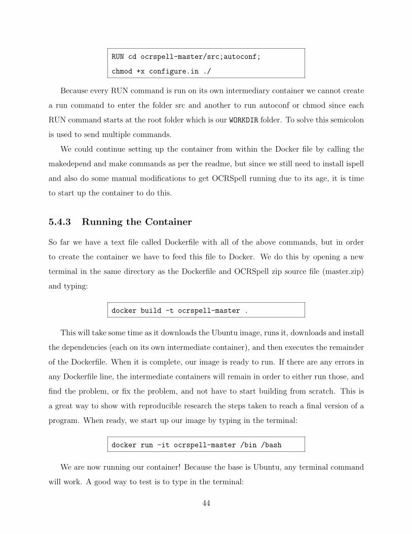
RUN cd ocrspell-master/src;autoconf;
chmod +x configure.in ./
Because every RUN command is run on its own intermediary container we cannot create
a run command to enter the folder src and another to run autoconf or chmod since each
RUN command starts at the root folder which is our WORKDIR folder. To solve this semicolon
is used to send multiple commands.
We could continue setting up the container from within the Docker file by calling the
makedepend and make commands as per the readme, but since we still need to install ispell
and also do some manual modifications to get OCRSpell running due to its age, it is time
to start up the container to do this.
5.4.3 Running the Container
So far we have a text file called Dockerfile with all of the above commands, but in order
to create the container we have to feed this file to Docker. We do this by opening a new
terminal in the same directory as the Dockerfile and OCRSpell zip source file (master.zip)
and typing:
docker build -t ocrspell-master .
This will take some time as it downloads the Ubuntu image, runs it, downloads and install
the dependencies (each on its own intermediate container), and then executes the remainder
of the Dockerfile. When it is complete, our image is ready to run. If there are any errors in
any Dockerfile line, the intermediate containers will remain in order to either run those, and
find the problem, or fix the problem, and not have to start building from scratch. This is
a great way to show with reproducible research the steps taken to reach a final version of a
program. When ready, we start up our image by typing in the terminal:
docker run -it ocrspell-master /bin /bash
We are now running our container! Because the base is Ubuntu, any terminal command
will work. A good way to test is to type in the terminal:
44

ls
It should show both our zip file source files and the unzipped directory. Now we can
install ispell by running in our terminal:
apt-get install ispell -yqq
This is the same command we would do in a regular Linux machine. After it is done
installing, we can test it by running:
ispell --help
Now it is time to finish building the source. First, let us enter the src folder.
cd ocrspell-master/src/
As the readme on github points out, due to the age of OCRSpell and deprecated code,
a few changes by hand must be made in order for the configure file to build correctly. First
lets open the file in nano:
nano configure
Then go to line 712 and change:
prefix=NONE
to
prefix=/home/ocrspell/ocrspell-master/src
Next, go to lines 732 and 733 and change:
datarootdir=’${prefix}/share’
datadir=’${datarootdir}’
to
45

datarootdir=’/home/ocrspell/
ocrspell-master/src’
datadir=’/home/ocrspell/
ocrspell-master/src’
respectively.
Save the file and close nano. Now we can run ./configure and then build as per the
readme with makedepend and make:
./configure --prefix=/local/ocrspell-master
makedepend
make
OCRSpell is now fully compiled and we can test it with the included test file called
quick demo.txt:
./ocrspell -a -f ./ocr.freq < quick d emo.txt
We have now successfully set up our container; however, due to the nature of the con-
tainer. If we were to close the container, we would lose all changes and the container would
open in the same state as if he had just done the Docker run command. So in order to save
our final container we can use the commit command in a different terminal window than
the one we are working with our container on. The syntax is:
docker commit <CONTAINER NAME FROM
DOCKER PS> <file name>
In this case we type:
docker ps
to find our Container name and then use the commit command with those values and a
name for our new container image. These names are randomly generated and change each
time we run the container so we must pay special attention to selecting the right one; in this
case it is distracted bardeen:
46

docker commit distracted bardeen
ocrspell-final
We now have a saved version of our container and can close the running container and
re-open it to the exact same state as it is now. To close it, in the terminal window where
our container is active we type:
exit
If we want to save our Docker image to share with other collaborators or publications we
use the save command:
docker save -o <save image to
path> <image name>
an example of this in our case is:
docker save -o /home/jfunlv/Desktop/
test/ocrspell-final ocrspell-final
Be sure to modify the first part with the path where we will save the image.
If there are any issues modifying the output image, use chmod and chown in linux to give
rights to it or the equivalent in other platforms.
If we want to upload to the Docker repository for other Docker users to collaborate or
reproduce our research we need to create a free Docker account at docker.com. Once we have
an account we have to tag and push the image. To do this we find the image id by typing:
docker images
Then, we tag the image by using:
docker tag 90e925195d6c username/
ocrspell-final:latest
Replace username with one’s Docker user name and replace the image id with that of the
appropriate image. Make sure one is logged in to Docker by typing:
47

docker login
Finally we push by:
docker push username/ocrspell-final
For full details on tagging and pushing see:
https://docs.docker.com/engine/getstarted/step six/
We have now uploaded a copy of our image for others to try, contribute and much more.
5.4.4 Downloading our version of the Container
The steps explained above should be done by the author of the research, but what if we want
to download someone else’s work and replicate it? In this case, we will download the image
that we created when writing this guide and run OCRSpell with a few simple commands.
We can download the image from an arbitrary location and load it up on Docker, or
download it from the official Docker git repository:
1. Load image in Docker: Suppose we downloaded from the author’s website an image
with a container to the project of OCRSpell. The file name is ‘ocrspell-image’
To load this image we open up a terminal at the image location and type:
docker load -i ocrspell-image
Make sure one is in the directory of the image otherwise type the path to it such as:
docker load /home/user/
Desktop/ocrspell-image
At this point we can type: docker images and verify that the entry was added. In
our case, ‘ocrspell-master’. As before we can now run it by typing:
docker run -it ocrspell- master /bin/bash
48

We now have a running container with OCRSpell that will not break or deprecate and
includes all necessary source and software to run.
2. Download directly to Docker from Docker git repository: To search from the available
images we use the ‘docker search command’ by typing the name of the image after the
search keyword:
docker search ocrspell
A list of matching images will appear. In this case, we want the ocrspell-master image
from the unlvcs user; to download it we use the pull command:
docker pull unlvcs/ocrspell-master
If we check docker images we should see it listed under the repository and can now
run it.
5.4.5 Deleting old images and containers
Once we are done working with an image we can use the docker rmi command followed by
the image ID that can be found next to the name of the image in docker images. In this
case, our Image id is: 90e925195d6c; therefore, we type in a terminal:
docker rmi 90e925195d6c
If there is a warning that the image is currently being used by a container. Make sure to
first close the container and then delete the image. If we want to delete all containers stored
in Docker we can do so by typing in a terminal:
docker rm $(docker ps -a -q)
Similarly, we can delete all images by typing:
docker rmi $(docker images -q)
49

5.4.6 Transferring files in and out of a container
So far only when executing the Dockerfile did we copy data onto the container. Ideally,
we want to copy all of our data at this time and store it within the container to have
everything in one place. But suppose that due to portability or projects with large file
size we want to maintain the data in a separate Docker container or repository in general.
Docker communications within containers can easily achieve this with the docker network
command. See for full details:
https://docs.docker.com/engine/userguide/networking/
If we want to instead transfer data from the container to, and from, the host machine,
we use the docker cp command.
5.4.7 Using the OCRSpell Container
Suppose we have an OCR document named FR940104.0.clean we would like to spell check
with OCRSpell. The document is in our host machine and we have pulled the latest version
of the OCRSpell container from the Docker repository. First we start our container by
running in a new terminal:
docker run -it unlvcs/ocrspell
-master /bin/bash
then we maneuver to the ocrspell program:
cd ocrspell-master/src
Next, we open a new terminal window at the location of our OCR document we will be
running and type:
docker ps
We find and save our container name there for ocrspell-final. In this case, its name is
adoring wescoff, but it will be different each time. We are now ready to copy the file into
the container. We run the following command:
50
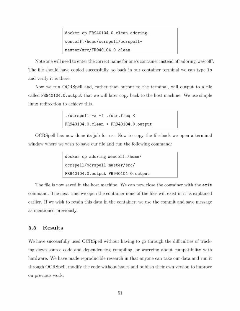
docker cp FR940104.0.clean adoring
wescoff:/home/ocrspell/ocrspell-
master/src/FR940104.0.clean
Note one will need to enter the correct name for one’s container instead of ‘adoring wescoff’.
The file should have copied successfully, so back in our container terminal we can type ls
and verify it is there.
Now we run OCRSpell and, rather than output to the terminal, will output to a file
called FR940104.0.output that we will later copy back to the host machine. We use simple
linux redirection to achieve this.
./ocrspell -a -f ./ocr.freq <
FR940104.0.clean > FR940104.0.output
OCRSpell has now done its job for us. Now to copy the file back we open a terminal
window where we wish to save our file and run the following command:
docker cp adoring wescoff:/home/
ocrspell/ocrspell-master/src/
FR940104.0.output FR940104.0.output
The file is now saved in the host machine. We can now close the container with the exit
command. The next time we open the container none of the files will exist in it as explained
earlier. If we wish to retain this data in the container, we use the commit and save message
as mentioned previously.
5.5 Results
We have successfully used OCRSpell without having to go through the difficulties of track-
ing down source code and dependencies, compiling, or worrying about compatibility with
hardware. We have made reproducible research in that anyone can take our data and run it
through OCRSpell, modify the code without issues and publish their own version to improve
on previous work.
51

As shown in this example, the steps taken to place OCRSpell into Docker are trivial and
mechanical. The complicated part was finding the dependencies and by-hand modifications
and making sure they were valid when first building the initial image. In new research, this
can be considered and easily stored in a Dockerfile making the added work to researchers
minimal. The Dockerfile itself is a great way to view the construction of the image, and
the container is a way to ensure that the reproducibility remains as it can be checked when
trying to rebuild the image to see if it matches.
5.6 Closing Remarks
This chapter reported on the state of reproducible research in document analysis and recog-
nition and its importance along with the challenges it brings. Docker containers are reviewed
as a solution to consistent reproducible research and a complete application is shown with
OCRSpell, a program that does not easily run in its current state, but after being placed in
a container is now immortalized to be able to be tested anywhere and anytime with ease.
Possible extensions to this project include parallel programming and complex GUI Docker
implementations examples, but more importantly, a proposed standard for reproducible re-
search for journal and conferences in this field with the hopes of a better future where we can
all share and work together to create good reproducible research that benefits the scientific
community.
52

Chapter 6
Methodology
Next, we will introduce the TREC-5 Data Set that was used for the multiple experiments.
Followed by that we discuss the de novo Alignment Algorithm for Ground Truth Generation
that was key for any additional experiments as this was a way to test the success of our
corrections. Then we discuss the Algorithm for using the Google Web 1T 5-Gram Corpus
for Context-Based OCR Error Correction. Before discussing it however, we introduce the
Google Web 1T 5-Gram Corpus and OCR Spell, two key data sets that are necessary to run
the Context-Based error correction.
6.1 The TREC-5 Data Set
When we were searching for a data set we could use for our ongoing OCR Post Processing
research, including the alignment part, we needed to have matching original and OCR’d
versions of the text that was both a large corpus, but could be split into smaller parts
we could test and compare. The U.S. Department of Commerce’s National Institute of
Standards and Technology (NIST) Text REtrieval Conference (TREC) TREC-5 Confusion
Track [55] was just what we needed. The following is an excerpt from the README file
contained in the TREC-5 Confusion Track file confusion track.tar.gz [111]:
“This is the document set used in the TREC-5 confusion track. It consists of
the 1994 edition of the Federal Register. The United States Government Print-
ing Office (GPO) prints the Federal Register as a record of the transactions of
53

the government. One issue is published each business day and contains notices
to Federal agencies and organizations, executive orders and proclamations, pro-
posed rules and regulations, etc. The Federal Register was selected for these
experiments because it is a large collection for which both hardcopy and elec-
tronic versions are readily available. The corpus contains 395MB of text divided
into approximately 55,600 documents.
There are three different text versions of the corpus. The “original” version is
derived from the typesetting files provided by the GPO; this is regarded as the
ground truth text version of the collection and was used to design the questions.
The “degrade5” version is the output obtained by scanning the hardcopy version
of the corpus. The estimated character error rate of this version of the corpus is
5%. The “degrade20” version was obtained by downsampling the original page
images produced above and scanning the new images. The estimated character
error rate of the downsampled images is 20%.”
For our purposes we have selected to work with the original and degrade5 versions as
they are the OCR generated errors that were naturally created when scanning the image and
converting it to text without the additional downsampling that generated more errors in the
degrade20 version. Each version is distributed into folders numbered 01-12 and within each
folder are files named “fr940104.0” where each file contains approximately 100 documents,
like “FR940104-0-00001”, separated by tags. Each document varies in length, but they are
approximately 1,000 words long, but with several larger ones with some being over 30,000
words long. This gives a great variety to experiment within the data set.
6.2 Preparing the Data set
As part of our larger project with the TREC-5 data set [36] we have created a MySQL
database where we insert the text files word by word without modifying much of the data
aside from basic cleanup that includes removing all tag data. The only tag data we use
before disposing of it is to separate individual documents within a file <DOCNO> so we can
annotate where each document begins and ends in the database along with its document
54
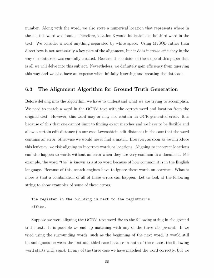
number. Along with the word, we also store a numerical location that represents where in
the file this word was found. Therefore, location 3 would indicate it is the third word in the
text. We consider a word anything separated by white space. Using MySQL rather than
direct text is not necessarily a key part of the alignment, but it does increase efficiency in the
way our database was carefully curated. Because it is outside of the scope of this paper that
is all we will delve into this subject. Nevertheless, we definitely gain efficiency from querying
this way and we also have an expense when initially inserting and creating the database.
6.3 The Alignment Algorithm for Ground Truth Generation
Before delving into the algorithm, we have to understand what we are trying to accomplish.
We need to match a word in the OCR’d text with the correct word and location from the
original text. However, this word may or may not contain an OCR generated error. It is
because of this that one cannot limit to finding exact matches and we have to be flexible and
allow a certain edit distance (in our case Levenshtein edit distance) in the case that the word
contains an error, otherwise we would never find a match. However, as soon as we introduce
this leniency, we risk aligning to incorrect words or locations. Aligning to incorrect locations
can also happen to words without an error when they are very common in a document. For
example, the word “the” is known as a stop word because of how common it is in the English
language. Because of this, search engines have to ignore these words on searches. What is
more is that a combination of all of these errors can happen. Let us look at the following
string to show examples of some of these errors,
The register in the building is next to the registrar’s
office.
Suppose we were aligning the OCR’d text word the to the following string in the ground
truth text. It is possible we end up matching with any of the three the present. If we
tried using the surrounding words, such as the beginning of the next word, it would still
be ambiguous between the first and third case because in both of these cases the following
word starts with regist. In any of the three case we have matched the word correctly, but we
55

may have matched to the incorrect location. Furthermore, if instead of the we had an OCR
generated error where h→n (h is misread as n. Therefore, the is misread as tne) and we
allowed an edit distance of 1 we could still match to any of the correct the. See Figure 6.1.
The register in tne building is next to the registrar’s office.
the tne
Figure 6.1: Both the and tne can match to any of the three the occurrences.
However, if the error was an i where the second character of a word starting with i was
either misread as a different character (s→g where is was misread as ig, or n→g where in
was misread as ig) or entirely deleted (s→ where is misread as just i) and we tried to match
it with an edit distance of 1 to the string we would not know which of the two candidates ‘is ’
or ‘in’ is the correct one since both are words in the ground truth sentence we are looking
at. It is also possible that in the unlikely error that s→n in our OCR’d text that we would
match to the incorrect word as in exists in the string as well as is. See Figure 6.2.
The register in the building is next to the registrar’s office.
i
Figure 6.2: With an edit distance of 1 i can match to either in or is.
Because of this, it is important to align not just to the correct word, but also to the correct
location. This is a key factor not just for ensuring we do not run into issues of aligning
to false positives, but also to greatly increase the alignment algorithm’s speed from the
‘non-deterministic polynomial time complete multiple string alignment problem’ to a more
56
manageable polynomial time complexity approach. We can do this by taking advantage that
statistically more words are correct than wrong in the OCR’d text. We know this because
the OCR’d text has an approximate error rate of 5% as given in the TREC-5 README
file [111], which is in line with state of the art OCR software. Furthermore, because the
OCR’d text, aside from column errors or other out of order text segments, should still be
in the overall same order and location as the correct ground truth text we can align words
in the order they appear. For words that do not have an OCR generated error they can be
used to help align ones that are not initially found due to errors. In the case that there are
shifts in locations due to insertions or deletions, the relative location between neighboring
words should remain similar as well allowing us to ensure we do not lose track of where the
matches are happening. For example, if we have the following two strings we are matching,
with the first one from the correct text, and the second one from the OCR’d text. Assuming
the initial locations of the first word on each text is 100 and 102 respectively,
The hegister in the building is next to the registrar is
office.
The register in the building is next to the registrar’s
office.
If we know that locations 100 (correct text) and 102 (OCR’d text) are a match for the
(there is already an ongoing shift in both texts due to missing or combined words in the
OCR’d text in comparison to the correct text) then we can initially assume that locations 101
and 103 should match (hegister and register) and so on. This will continue until locations
108 and 110 (the for both texts); however, locations 109 and 110 in the OCR’d text (registrar
and is) are words that should both match to location 111 in the correct text (registrar’s).
This can pose a challenge of its own as well, but ultimately it is to our advantage to use
the preceding aligned words to assist in aligning the succeeding words. Do note that at the
end of both sentences the location of the word office is 111 in the OCR’d text and 112 in
the correct text. This means that the location shift between both text – for matching word
57

locations – has decreased from 2 to 1. This shows how the overall alignment of both texts
can slowly change, or shift/drift, due to missing or combined words. One way to control
this is to separate documents into their own contained files rather than one very long corpus
with no separations and a large number of documents.
With this we present the algorithm starting at the beginning of both corpus pointing to
what we believe to be the first word of the OCR’d text and the original/correct text:
0. We assign a confidence weight to each word we will process that will store how confident
we are that the current word was aligned to the correct word/location. This weight
will vary whether it was an exact match (potentially no OCR generated errors) or a
match after edit distance was applied (in which case the word has one or more OCR
generated errors). Initialize the confidence for all words to 0.
1. Take the next OCR’d word and check against a dictionary to see if it is a real word.
If it is then increase confidence by .5 and continue to step 2.
2. Check the previous word we aligned for the last location. (0 if this is first word). Using
that location, we check the immediate next word in the correct text to see if it is a
match.
• If it is a match we increase both this word confidence and the previous by .25
Then we are done aligning. Store the location found in the database and move
on to the next word (start over in step 1).
• If it is not a match we decrease the confidence of this word by .25 and if the
current confidence of this word was .5 (was match in dictionary) then we decrease
the confidence of the previous word by .25 and continue to step 3.
3. Since it was not a match we begin to look for the word in a nearby location: We search
for exact matches after the word for X words (X for now is 20 words).
• If we find a matching candidate, we increase the confidence by .25 and move on
to the next word.
58

• If we do not find a matching candidate we search X words before the previous
word.
• If we find a matching candidate we increase the confidence by .1 and decrease the
confidence of the previous word by .4 and move on to the next word.
• Else go to step 4.
4. No match for words either immediately after or in the neighboring X words: We are
going to search for matches like in step 3 for neighboring words but rather than search
for exact matches we are going to search for words that have an edit distance of Y. Y
can be greater than 1 but we will iterate starting with 1 edit distance until Y. Great
care must be taken to limit the size of Y to avoid false positives. For now, we will set
a maximum Y of 3:
While edit distance checked is less than Y:
• If we find a matching candidate with Y distance, we increase the confidence by .1
and move on to the next word.
• If not then we increase the edit distance (Y++) and continue loop.
5. Once we exhausted our edit distance allowed, if we have not found a word we then
search in a similar fashion for the previous X words (as we did in step 3, but in this
case allowing an edit distance until Y).
6. If after all this we do not find a match. Then we give it a confidence of -1 and store
the location of the previous word plus 1. We mark in the database as well that the
word failed to be aligned so we can ensure that when we are testing OCR data we can
handle either not using that word for testing or try to align it using something else.
We also keep a counter of match failures and if we have more than Z in a document (so
20 in our case) we warn the user to take a closer look to identify the problem as most
likely the alignment has lost its way because of out of order text or other unforeseen
circumstances.
59
We continue this algorithm until we have reached the end of the document we are aligning.
If we are aligning more than one document at a time, due to the way the data is stored we
are always able to start at the beginning word of both documents which may or may not be
a match but does guarantee that any alignment problems from one document do not bleed
into the other. Lastly, the algorithm as implemented reads from the database by chunks in
order to avoid huge number of queries and work efficiently with a database of any size, but
does not commit changes until it is done.
6.4 OCR Spell
In the previous chapter on Reproducible Research in Document Analysis and Recognition, we
were able to take the old source code, compile it after installing the necessary dependencies,
and sucessfully run it in a Docker container that we later uploaded for everyone to easily
download and use. This is due to Docker greatly enabling and encouraging reproducible
research through the use of container technology [8].
For this project, we used OCRSpell to detect OCR generated errors along with a way to
benchmark our correction against OCRSpell and to then try and complement it as a way
to select the best candidate suggested by OCRSpell. The ease in which we were able to use
OCRSpell in this project is a good example on why reproducible research allows building on
top of previous work very easily and increases its relevance to scientists. During our work
with OCRSpell, we detected a bug when using a single quote ( ’ ) surrounded by white space
or by other quotes that were surrounded by whitespace. This is most likely a parsing error
that we intend on fixing for the benefit of the community. This shows that as Peng points
out, “reproducibility is critical to tracking down the ‘bugs’ of computational science” [79].
6.5 Google Web-1T Corpus
The Google Web 1T 5-gram Version 1 corpus (Google-1T) is a data set “contributed by
Google Inc., contains English word n-grams and their observed frequency counts. The length
of the n-grams ranges from unigrams (single words) to five-grams” [11]. For the purposes of
this paper we will be using the unigrams (1-grams) and trigrams (3-grams). The unigrams
60

serve as a dictionary of all words contained in the data set. The trigrams will server as our
context. The source of the data, “The n-gram counts were generated from approximately 1
trillion word tokens of text from publicly accessible Web pages” [11].
What makes Google-1T great is that having it based on Web pages allows it to have a
broader variety of subjects that enable it to understand more context than other corpus. The
variety does come at a price, as n-grams with fewer than 40 occurrences are omitted [27].
This means that many correct 3-grams that could be very specialized to a topic are missing.
A possible solution to this would be to add subject-specific 3-grams to the data set for the
documents being corrected. There are 13,588,391 unigrams and 977,069,902 trigrams in the
corpus contained in approximately 20.8 GB of uncompressed text files.
6.6 The Algorithm for Using the Google Web 1T 5-Gram Corpus
for Context-Based OCR Error Correction
In this algorithm we use the idea of context-based orthographic error corrections by taking
the TREC-5 Confusion Track Data Set’s degrade5 and attempting to correct errors generated
during Optical Character Recognition. We do this by first identifying all errors using OCR-
Spell. Next, we generate the 3-gram by searching for the first and last word in the Google
Web 1T corpus of trigrams. We then select the candidates with the highest frequencies and
a small Levenshtein edit distance. Finally, we report on our accuracy and precision and
discuss on special situations and how to improve performance. All source code is publicly
available for our readers to further our work or critique it.
6.6.1 Implementation Workflow
The workflow of our algorithm and run-script is as follows. Start with OCR’d text and
identifying OCR errors, we then generate 3-grams for each error, search in Google-1T for
3-grams where the first and third word match the given 3-gram and then pick the one with
the highest frequency as our top candidate if any. Finally, we verify the output using an
alignment algorithm we developed [35] that will align the original text with the OCR’d text
to generate statistics on the accuracy of our solution. The implementation is split into several
61

modules that perform the aforementioned tasks:
6.6.2 Preparation and Cleanup
This pre-processing step transforms the TREC-5 files into clean, human-readable documents.
Initially the TREC-5 Data set contains several tags like <DOC>, <DOCNO>, <SUMMARY>
that are markers for programs and not actual content to be used for 3-gram collection and
thus can be safely removed. We do take advantage of the <DOCNO> to denote where each
Document begins and ends since each text file in TREC-5 contains 100 individual documents.
Separating them makes it easier to split and transfer into the OCRSpell container we will
use in the following steps. These tags are in both the degrade5 and original copies of the
files. In the original TREC-5 files there are additional HTML-style character references
such as & and &hyph;. These character references can be handled in a variety of ways
depending on what it represents. For this step, we take the common ones and transform
them into the ASCII character they represent. It is important to point out that our results
could be improved by handling these character references with more care than eliminating
them or replacing them, but doing so would bias our results to look better with this data
set than any other data set that could be thrown into our program. Therefore, it is best
to remain as neutral as possible. At the end of this step, our tidy data [118] is ready to be
transferred into an OCRSpell container.
6.6.3 Identifying OCR Generated Errors Using An OCRSpell Con-
tainer
In order to identify what words are errors we send our split files into a Docker container
running an instance of OCRSpell. OCRSpell then generates an output file where each line
represents the next word, separated by whitespace, in the given documents. If the word is
correct it marks an asterisk (*), if the word is incorrect and has no suggestions it marks
a number sign (#), and if the word is incorrect and has suggestions/candidates it marks
an ampersand (&) followed by the candidates. The first line of OCRSpell has information
about the program and is preceded by an at sign (@).
62

@(#) Ispell Output Emulator Version 1
* ← Correct Word
& ← Incorrect Word with Suggestions
# ← Incorrect Word with No Suggestions
For example, here are the first few lines of the first OCRSpell output file from the first
document, degrade.FR940104-0-00001.000.output:
@(#) Ispell Output Emulator Version 1
*
& hegister 2 0: register, heister
*
# 391 0
*
# 2 0
*
& anuary 1 1: January
# 41 0
The matching text for this file is found in degrade.FR940104-0-00001.000:
Federal hegister Vol. 391 No. 2 )
Tuesday1 ’anuary 41 1994 hules and
The word hegister is identified as misspelled and OCRSpell has two candidates. It orders
them by likeliness that they are the correct answer. In our experiment, we only care about
identifying the word as incorrect and not using the candidates offered. However, in future
experiments we will be using this data along with this experiment’s output to increase
efficiency. Furthermore, numbers are identified as misspellings with no candidates. In our
63

next section, we must take this into consideration and skip numerical words as they are
assumed to be correct. Also notice that the word anuary should match ’anuary but it does
not because OCRSpell has done pre-processing on this word and removed punctuation. This
is an issue when trying to align our words that we deal with in a later section. Finally,
notice that the single character ‘)’ should be classified as a word but is instead ignored
and discarded by OCRSpell. This causes alignment problems with the amount of lines in
OCRSpell not matching the number of words in the documents fed to OCR Spell. This is
dealt with in the next section.
6.6.4 Get 3-grams
Once we generate the OCRSpell output and copy it back from the container to the host ma-
chine we use this to locate the misspelled words in the cleaned texts by using the line as the
location in the document. We then collect the neighboring words to form the 3-grams whose
middle word is the incorrectly spelled word and continue on to the next misspelled word.
For now, this process is sensitive to the choices made by OCRSpell. If OCRSpell chooses to
ignore a word, then the discrepancy between the cleaned form of the source document and
the OCRSpell output will increase the error rate by producing erroneous 3-grams. We ignore
any 3-grams with a number as the second center word because a number is value-specific
and we cannot know which value it is supposed to take. As mentioned earlier, this could be
improved by replacing and merging frequencies in the Google-1T data set that involve special
phrases. In the second version of our code, we implement a crude version of our alignment
algorithm [35] to overcome the alignment problem and properly generate 3-grams without
errors. In this relatively simple case we were able to achieve 100% accuracy on re-aligning
OCRSpell output with the given clean text files as long as the Levenshtein edit distance was
smaller than the threshold. Because most OCR words have a small number of errors this
covers most cases. In our third version of the code we wanted to make sure that, alignment
or not, we could guarantee all matches so we implemented our own Spell Checker that uses
the Google Web 1T 1-gram vocabulary which has all words that appear in the corpus, sorted
alphabetically, to identify if a word has an error and ensure that for every word in the text
there is a corresponding line generated in our output that mimics the OCRSpell formatting
64

to ensure 100% alignment:
@(#) Google 1T OCRSpell Output Emulator
*
# hegister 0
*
# 391 0
*
# 2 0
*
*
# ’anuary 0
# 41 0
Notice that here we have the additional line with asterisk to indicate that the single paren-
thesis is considered a word, since it is separated with whitespace, that is correct. Also note
that we do not generate candidates so we mark all errors with the number sign. Everything
is done with the same format as OCRSpell.
Here is an example of an output file after we have generated the corresponding 3-grams
for all Errors. The following is from Version 3 using 1-grams to mimic OCRSpell for file
degrade.FR940104-0-00001.000.3gms:
Federal hegister Vol. 1
Tuesday1 ’anuary 41 8
and hegulations Vol. 13
Tuesday1 ’anuary 41 19
After we have generated all 3-grams we can then move on to searching the Google1T
data set.
65

6.6.5 Search
For this step, we consult Google Web 1T to produce a list of candidate 3-grams for each
erroneous word. Since the Google1T database is stored as a list of indexed files, we utilize
the index to quickly locate which file(s) our 3-grams may be in. Note that it is possible
that the 3-grams candidates may be in multiple Google1T files due to them being near the
end of one file or in the beginning of another. Realistically, in the worst case, they are in
2 files at the most and even so this is very rare. Once we’ve collected the names of the
files, to we utilize bash’s grep tool to search each file for all the 3-grams whose first and
last word match those of our 3-gram. We then save these candidates as potential correc-
tions for our misspelled word. The output file is separated into sections whose beginning
is marked by a line with a sequence of characters “%%%” followed by the 3-gram of an
incorrectly spelled word. Subsequent lines before the next section are the Google1T 3-grams
with the candidate correction at the center. The following is an excerpt of the results from
degrade.FR940104-0-00001.000.candidates:
%%% Federal hegister Vol. 1
Federal Domestic Volunteer 76
Federal Employee Volunteer 42
Federal Loan Volume 47
Federal Register Vol 8908
Federal Register Vol.59 41
Federal Register Vol.60 75
Federal Register Vol.61 81
Federal Register Vol.62 83
Federal Register Vol.63 69
Federal Register Vol.65 82
Federal Register Vol.66 57
Federal Register Vol.70 63
Federal Register Volume 1833
66

Federal Regulations Volume 68
Federal Reserve Volume 8013
Federal Surplus Volunteer 380
%%% Tuesday1 ’anuary 41 8
%%% and hegulations Vol. 13
and destroy Voldemort 67
and development Vol 58
rest of output truncated*
As we can see the first 3-gram generated 16 candidates of which the most frequent
is Federal Register Vol with 8908 frequency. On the opposite end, the next 3-gram
generated no candidates due to having an error in a neighboring word. This could be fixed
with multiple passes and allowing edit distance in the 3-gram generation but would greatly
increase the number of candidates generated and the runtime. Something for the future. The
next 3-gram after that generated over 2000 candidates due to having such common words as
the first and third word and hegulations Vol.. To solve this issue we reduce the number
of candidates each 3-gram generates in the next step.
6.6.6 Refine
Currently any word, regardless of edit distance, appears in our candidate list of 3-grams.
However, it is unlikely that the correct word has a large edit distance compared to the can-
didates so in the refine step we eliminate candidates with large Levenshtein edit distances
even if they have high frequency. Test indicated this to be the case. Doing so reduced our
candidate list to a more manageable size at the cost of some 3-grams losing all available
candidates the more the edit distance is restricted. Here is the output on the same file we
have shown degrade.FR940104-0-00001.000.clean:
%%% Federal hegister Vol. 1
Federal Register Vol 8908
Federal Register Vol.59 41
67

Federal Register Vol.60 75
Federal Register Vol.61 81
Federal Register Vol.62 83
Federal Register Vol.63 69
Federal Register Vol.65 82
Federal Register Vol.66 57
Federal Register Vol.70 63
Federal Register Volume 1833
&&& Register
%%% Tuesday1 ’anuary 41 8
&&&
%%% and hegulations Vol. 13
and Regulations Volume 146
&&& Regulations
%%% Tuesday1 ’anuary 41 19
Another addition to refine is a list of candidates beneath all the remaining 3-grams sorted
by highest frequency appearing first for multiple candidates. We can see that the first 3-gram
has only 1 candidate left which happens to be the correct answer. Our testing indicated that
an edit distance of 4-5 is the ideal values in terms of having about 70-80% of all the 3-grams
that originally had candidates keep at least 1 candidate. This was taking into consideration
3-grams with candidates that were all false positives or incorrect candidates. As mentioned
before it is far easier to correct large words as smaller words can be greatly mutated with a
small edit distance. Ideally, we could have a variable edit distance depending on the length
of the word.
6.6.7 Verify
Finally for the last step we want to take the original file and compare it to our candidates
and corrections in order to produce statistics to verify our correction accuracy. This is
accomplished by consulting a document with each incorrect word mapped to its correct
68

version. This document was generated as part of our alignment algorithm project for the
same data and comes from a MySQL database with all of the documents. The Alignment
allows for text to be out of order and not aligned due to extra words added the OCR’d text
or words missing in the OCR’d text [35]. Using this data, we count how many words were
corrected properly and how many at least had the correct word in its candidate list. This
information is saved to a file with the filename, count corrected, and count of words with
correct word in suggestions on a single line for further analysis.
69

Chapter 7
Results
Next, we will discuss the resulting performance of the alignment algorithm for ground truth
generation. This is followed by the results of Using the Google Web 1T 5-Gram Corpus for
OCR Context Based Error Corrections.
7.1 Performance and Analysis of the Alignment Algorithm for
Ground Truth Generation
Using the first 100 documents in the TREC-5 Database, we insert 153,454 words in the
database from the original/correct text. We then insert 155,282 words in the database from
the corresponding OCR’d text. This already tells us that there are over 1,800 additional
words in the OCR’d text. We then run the algorithm and compute the average success rate,
which we define as
Number of Words Aligned Successfully
Total Number of Words Attempted= Success Rate
This returns us a success rate of 81.07% for the 155,282 words processed. With the total
amount of match failures at 29,397. At first, this may seem like a low number as this means
that nearly 1 of every 5 words failed to be aligned. However, we must understand that the
theoretical limit due to the discrepancy in word count between the degraded and original
texts is
153, 454
155, 282× 100% = 98.823%
70

More importantly, analyzing the individual document success rate, see Figure 7.1.
Figure 7.1: Individual Document Success Percentage Rate.
Summary:
Total Match Failures: 29,397
Number of words processed: 155,282
Average Success Rate: 81.07%
Lowest Individual Success Rate: 66.12%
Highest Individual Success Rate: 100.00%
We can see that the majority of the documents had a very high success rate over 90.00%,
the only documents with a success rate lower than that were the following 15 documents,
66.12%, 66.54%, 66.75%,
66.79%, 67.33%, 68.22%,
70.25%, 71.83%, 72.49%,
73.54%, 80.73%, 85.34%,
86.36%, 86.49%, 86.71%
Looking at several of these more carefully,
Processing Document: FR940104-0-00008
Degrade Range [3216,3892] and Original Range [3172,3868].
71

Match Failures: 229. Local Success Rate in Document: 66.12%
Processing Document: FR940104-0-00021
Degrade Range [14433,15210] and Original Range [14328,15092].
Match Failures: 260. Local Success Rate in Document: 66.54%
Processing Document: FR940104-0-00027
Degrade Range [18021,18479] and Original Range [17866,18219].
Match Failures: 126. Local Success Rate in Document: 72.49%
Processing Document: FR940104-0-00028
Degrade Range [18480,19235] and Original Range [18220,18773].
Match Failures: 251. Local Success Rate in Document: 66.75%
Processing Document: FR940104-0-00029
Degrade Range [19236,19914] and Original Range [18774,19242].
Match Failures: 191. Local Success Rate in Document: 71.83%
Processing Document: FR940104-0-00030
Degrade Range [19915,20668] and Original Range [19243,19782].
Match Failures: 224. Local Success Rate in Document: 70.25%
Processing Document: FR940104-0-00031
Degrade Range [20669,26255] and Original Range [19783,25111].
Match Failures: 1775. Local Success Rate in Document: 68.22%
Processing Document: FR940104-0-00032
Degrade Range [26256,49803] and Original Range [25112,48504].
Match Failures: 7692. Local Success Rate in Document: 67.33%
Processing Document: FR940104-0-00033
Degrade Range [49804,68849] and Original Range [48505,67470].
Match Failures: 5040. Local Success Rate in Document: 73.54%
Processing Document: FR940104-0-00034
Degrade Range [68850,105839] and Original Range [67471,104343].
Match Failures: 12283. Local Success Rate in Document: 66.79%
We see a set of them located near each other with some of the documents having a large
72

amount of words in them. Document FR940104-0-00034 has 36,872 words of which 12,283
were failures. This single document accounts for over 41% of the failures found and along
with the previous two documents with 7,692 and 5,040 match failures account for a total
of 85.10% of the match failures and for a total of 79,231 words which is over half of the
words. Analyzing these files we find that the top reasons for match failures were out of
order text due to zoning problems such as a column misread or image captions and data
being in a different order between both files, and misalignment where the threshold that
we had for checking neighboring words became greater than the program allowed. This is
bound to happen with larger files where not everything is aligned. The files also contain
a lot of numerical and special character data that the OCR software appears to have had
issues processing therefore creating a lot of OCR generated errors. In all of these cases,
the alignment algorithm failed to work when the errors created a greater discrepancy than
the threshold allowed. At that point when the alignment was so misaligned it could not
reset itself, would then cascade into more mismatches until the end of the document. The
Alignment algorithm ‘lost its way’ midway. If we were to be able to solve the issue by only
trying to search through the entire document after the algorithm is determined to have lost
its way we could salvage the matching and greatly increase our success rate. As we can see
in documents where the alignment algorithm did not lose its way, those that were above 90%
success rate, which accounts for an 85% of the documents, had an average success rate is
98.547% Meaning that if we can solve the issues mentioned, primarily the occasional out of
order text problem above we can get as close to the theoretical limit as 0.0276%.
Original Text for DOCNO FR940104-0-00001:
<DOC>
<DOCNO> FR940104-0-00001 </DOCNO>
<PARENT> FR940104-0-00001 </PARENT>
<TEXT>
<!-- PJG FTAG 4700 -->
<!-- PJG STAG 4700 -->
73

<!-- PJG ITAG l=90 g=1 f=1 -->
<!-- PJG /ITAG -->
<!-- PJG ITAG l=90 g=1 f=4 -->
Federal Register
<!-- PJG /ITAG -->
<!-- PJG ITAG l=90 g=1 f=1 -->
␣/␣Vol. 59, No. 2␣/␣Tuesday, January 4,
1994␣/␣Rules and Regulations
<!-- PJG 0012 frnewline -->
<!-- PJG /ITAG -->
<!-- PJG ITAG l=01 g=1 f=1 -->
Vol. 59, No. 2
<!-- PJG 0012 frnewline -->
<!-- PJG /ITAG -->
<!-- PJG ITAG l=02 g=1 f=1 -->
Tuesday, January 4, 1994
<!-- PJG 0012 frnewline -->
<!-- PJG 0012 frnewline -->
<!-- PJG /ITAG -->
74

<!-- PJG /STAG -->
<!-- PJG /FTAG -->
</TEXT>
</DOC>
Cleaned Up File Inserted to Database for DOCNO FR940104-0-00001:
Federal Register
␣/␣Vol. 59, No. 2␣/␣Tuesday, January 4,
1994␣/␣Rules and Regulations
Vol. 59, No. 2
Tuesday, January 4, 1994
OCR’d Text for DOCNO FR940104-0-00001:
<DOC>
<DOCNO> FR940104-0-00001 </DOCNO>
<TEXT>
Federal hegister ) Vol. 391 No. 2 )
Tuesday1 ’anuary 41 1994 ) hules and
hegulations
Vol. 391 No. 2
Tuesday1 ’anuary 41 1994
</TEXT>
</DOC>
75

Cleaned Up File Inserted to Database for DOCNO FR940104-0-00001:
Federal hegister ) Vol. 391 No. 2 )
Tuesday1 ’anuary 41 1994 ) hules and
hegulations
Vol. 391 No. 2
Tuesday1 ’anuary 41 1994
The following queries show the database tables where the algorithm reads the text files from
and writes the alignment output to. These samples are all based on the same DOCNO
FR940104-0-00001 for both Original and OCR’d text:
USE TRECSample;
SELECT * FROM doctext LIMIT 24; -- (See Table 1 for
output)
SELECT * FROM doctextORIGINAL LIMIT 19; -- (See Table 2)
SELECT * FROM matchfailList LIMIT 1; -- (See Table 4)
SELECT * FROM docErrorList LIMIT 14; -- (See Table 3)
SELECT * FROM doctextSolutions LIMIT 24; -- (See Table 5)
76

Table 7.1: doctext
word location locationOR docsourceFederal 0 0 FR940104-0-00001hegister 1 1 FR940104-0-00001) 2 14 FR940104-0-00001Vol. 3 11 FR940104-0-00001391 4 12 FR940104-0-00001No. 5 13 FR940104-0-000012 6 14 FR940104-0-00001) 7 17 FR940104-0-00001Tuesday1 8 15 FR940104-0-00001’anuary 9 16 FR940104-0-0000141 10 17 FR940104-0-000011994 11 18 FR940104-0-00001) 12 14 FR940104-0-00001hules 13 15 FR940104-0-00001and 14 9 FR940104-0-00001hegulations 15 10 FR940104-0-00001Vol. 16 11 FR940104-0-00001391 17 12 FR940104-0-00001No. 18 13 FR940104-0-000012 19 14 FR940104-0-00001Tuesday1 20 15 FR940104-0-00001’anuary 21 16 FR940104-0-0000141 22 17 FR940104-0-000011994 23 18 FR940104-0-00001
Table 7.2 is the original text and Table 7.1 is the OCR’d text. The tables contain the
word, its location in the file, such as first, second, or 100th word, and in the case of the
OCR’d text table, contains the aligned location after alignment has been run. Table 7.5 is
the updated table after the alignment algorithm is completed. The column word is OCR’d
Text word in the location shown, and the column wordOR is the word from the Original
Text file that it was aligned to. The column location shows the OCR’d Text location for
that word and the column locationOR shows the matching location from the Original file.
As we can see the majority of the words were matched to the correct words regardless if
they had an OCR error that was generated during the conversion. The only match failure
was hules not being matched with Rules because it was not inserted into the database
correctly. In this case, the word Unknown is written into wordOR and this location is added
77

Table 7.2: doctextORIGINAL
word location docsourceFederal 0 FR940104-0-00001Register 1 FR940104-0-00001␣/␣Vol. 2 FR940104-0-0000159, 3 FR940104-0-00001No. 4 FR940104-0-000012␣/␣Tuesday, 5 FR940104-0-00001January 6 FR940104-0-000014, 7 FR940104-0-000011994␣/␣Rules 8 FR940104-0-00001and 9 FR940104-0-00001Regulations 10 FR940104-0-00001Vol. 11 FR940104-0-0000159, 12 FR940104-0-00001No. 13 FR940104-0-000012 14 FR940104-0-00001Tuesday, 15 FR940104-0-00001January 16 FR940104-0-000014, 17 FR940104-0-000011994 18 FR940104-0-00001
Table 7.3: docErrorList
word location docsourcehegister 1 FR940104-0-00001) 2 FR940104-0-00001391 4 FR940104-0-00001) 7 FR940104-0-00001tuesday1 8 FR940104-0-00001’anuary 9 FR940104-0-0000141 10 FR940104-0-00001) 12 FR940104-0-00001hules 13 FR940104-0-00001hegulations 15 FR940104-0-00001391 17 FR940104-0-00001tuesday1 20 FR940104-0-00001’anuary 21 FR940104-0-0000141 22 FR940104-0-00001
to the matchfailList table. See Table 7.4. Words that are aligned but have an edit distance
of 1 or more are also inserted into the docErrorList table, See Table 7.3, as they contain
78

Table 7.4: matchfailList
word location docsourcehules 13 FR940104-0-00001
Table 7.5: doctextSolutions
word wordOR location locationOR docsourcefederal federal 0 0 FR940104-0-00001hegister register 1 1 FR940104-0-00001) 2 2 14 FR940104-0-00001vol. vol. 3 11 FR940104-0-00001391 59, 4 12 FR940104-0-00001no. no. 5 13 FR940104-0-000012 2 6 14 FR940104-0-00001) 4, 7 17 FR940104-0-00001tuesday1 tuesday, 8 15 FR940104-0-00001’anuary january 9 16 FR940104-0-0000141 4, 10 17 FR940104-0-000011994 1994 11 18 FR940104-0-00001) 2 12 14 FR940104-0-00001hules Unknown 13 15 FR940104-0-00001and and 14 9 FR940104-0-00001hegulations regulations 15 10 FR940104-0-00001vol. vol. 16 11 FR940104-0-00001391 59, 17 12 FR940104-0-00001no. no. 18 13 FR940104-0-000012 2 19 14 FR940104-0-00001tuesday1 tuesday, 20 15 FR940104-0-00001’anuary january 21 16 FR940104-0-0000141 4, 22 17 FR940104-0-000011994 1994 23 18 FR940104-0-00001
at least one OCR generated error since they were not found in the database. As we can
see some of the words aligned to an incorrect instance of the word due to invalid tag data
being read into the database. This shows that the algorithm will search for and try to latch
on to nearby groups of words that could match the OCR’d text before giving up. In this
case, it successfully did this. If we wanted to avoid the original issue we would have to
clean the text further by considering ␣ as tag data and automatically replace it with
whitespace so text could be read properly into the database. Finally, Table 7.6 provides a
visual representation of the doctextSolutions table and aids in showing how the alignment
79

of both text files jumps around into 2 major contigs, 1 small one and 3 individual words
aligned.
Table 7.6: First Number Represents location in OCR’d Text, Second Number Representslocation in Original Text.
Alignment OutputCorrect Text from Source File
wo
rd
Federa
l
Regis
ter
&bla
nk
59,
No.
2&
bla
nk;/&
bla
nk;T
uesday,
January
4,
1994&
bla
nk
and
Regula
tions
Vol.
59,
No.
2 Tuesday,
January
4,
1994
OC
R G
en
era
ted
Co
nvers
ion
Text
word
Federal 0,0
hegister 1,1
) 2,14
Vol. 3,11
391 4,12
No. 5,13
2 6,14
) 7,17
Tuesday1 8,15
'anuary 9,16
41 10,17
1994 11,18
) 12,14
hules ? X
and 14,9
hegulations 15,10
Vol. 16,11
391 17,12
No. 18,13
2 19,14
Tuesday1 20,15
'anuary 21,16
41 22,17
1994 23,18
7.2 The Results of Using the Google Web 1T 5-Gram Corpus for
OCR Context Based Error Correction
For the three runs performed. More than triple the amount of words were corrected in the
OCR Aligned run versus the Non-Aligned run. This may seem surprising seeing how little
the percentage of OCR Errors detected changed, but is not because we no longer have invalid
3-grams that never existed in the original text or the OCR’d Text.
80

Surprisingly the 1-gram Aligned method performed less than the OCR Aligned method
and is more due to the limited vocabulary from which it can detect errors. However, this
version is the one that has the greatest room for improvement, as it is a mere comparison
to the vocabulary list. For words that the correct version exists in the Google1T 1-gram
vocabulary, the main reasons why they were unable to generate the correct candidate were:
• Mistakes in neighboring words to the 3-gram: If we have two or three words that have
OCR Generated Errors in them then matching to valid 3-grams is very unlikely. A
solution to this as mentioned would be to match to 3-grams with a short edit distance
whenever there are no candidates. Also doing several passes of the algorithm to slowly
fix words one at a time. This would require to do 3-grams where the misspelled word
could appear as the first or third word and to use the other two as context.
• Numbers in Neighbor words: OCRSpell removes numbers and punctuation in a word
before checking if it is spelled correctly. Doing this is good; however unless we also do
that in our code then we face trying to find 3-grams with words that have numbers as
part of the word.
• Not a word: Numbers or combination of numbers and letters like, SFV93-901-1An or
US.C.001014 are practically impossible to find even if we had Levenshtein. These sets
of letters could be valid, or invalid, in the original file and may create false positives.
• Hyphens between words: For example, “California-Arikona” has issues because the
Google1T data set separated those words with hyphens into separate words so not
only does that word have a spelling mistake, but it would also be more scarce to find
such 3-grams.
• Rare words: Especially for 1-gram search. Google1T has a limit of not showing words
with frequencies lower than 40. Therefore, a lot of valid but rare or specialized words
will not appear in the corpus and in that case.
• False Negatives are also present when a word that has an OCR Generated Error is
marked as correct when the word itself is valid but not what was originally intended.
81

An example of this was the word “hules” in the first document. The correct word is
rules but hules is a valid word and is marked as OK by 1-gram search but not by
OCRSpell. A solution to this would be to use a confusion matrix to check if a word is
misspelled.
• Acronyms in both neighboring words when generating the 3-grams or as the word
being identified if correct or not pose a problem in detecting. One solution would be
to implement the old Acronym finder to recognize these as acronyms and leave them
alone [101].
A: Non-Aligned OCRSpellB: Aligned OCRSpell
C: Aligned 1-gram Mimicking OCRSpell
C
B
A %
%
%
35.55
48.44
32.34
Figure 7.2: Percentage of Identified OCR Generated Errors with Candidates (After Refine).
A: Non-Aligned OCRSpellB: Aligned OCRSpell
C: Aligned 1-gram Mimicking OCRSpell
C
B
A %
%
%
13.74
26
13.87 C
B
A %
%
%
4.36
14.35
8.09
(a) (b)
Figure 7.3: Percentage of Identified OCR Generated Errors with Candidates that includethe correct word (after refine) (a). Percentage of those that include the correct word as thefirst suggestions (b).
As Gritta et al. state, “If research is optimised towards, rewarded for and benchmarked
82

on a possibly unreliable or unrepresentative dataset, does it matter how it performs in the
real world of Pragmatics?” [37]. Several papers have reportedly shown higher correction
success rates using Google1T and n-gram corrections [6, 69] than our results. Unlike those
cases, we publicly provide our data and code.
83

Chapter 8
Post-Results
In this chapter we discuss the results of the Alignment Algorithm for Ground Truth Gen-
eration. We place special emphasis on analyzing the results with the goal of improving the
alignment algorithm for special cases that cover the major cluster of issues. We then focus
on a discussion in regards to finding a solution to zoning problem. Next, we discuss the
challenges, planned improvements, and possible future work on Using the Google Web 1T
5-Gram Corpus for Context-Based OCR Error Correction.
8.1 Discussion on the Results of the Alignment Algorithm for
Ground Truth Generation
8.1.1 Improvements for Special Cases
The main issue we are facing in our alignment is when there is out of order text. Typically
such problem comes when something like two columns are read as one while generating the
OCR’d text file. Another example is when a caption from an image is read in as part of the
regular text. This problem is exactly what we are facing, but in a different situation. In this
case, the OCR tool used to create the TREC-5 database did a good job at reading columns
correctly. The problem lies in the original document. The original TREC-5 Files have
tags for FOOTNOTES, captions and other special text locations that allow the parser that
created the prints to place this text in the correct places. Nevertheless, because those tags
allow the writer to place these tags anywhere in the source files, they can place a footnote tag
84

with the according text in the middle of the page. Because we ignore tag information when
cleaning up the data in the beginning, we end up with such text out of order. The simple
solution would be to add a tag exception when cleaning up the text or to tag that data in
our database as a potential caption or table name in order to process it more carefully and
check against mismatched text. This would work perfectly, but this would overspecialize
our algorithm for just this data set and would not work with other data sets that may
actually have out of order text causing zoning problems. We could use a heuristic approach
to generate our own tags such as in Autotag [99] which is part of MANICURE designed at
ISRI [93, 94, 100], but to use this we would have to generate data for the entire document,
and while this may give us better results, it is possible we would lose efficiency, so while we
can take some ideas from these past projects, another solution must be found that will work
in all cases where text is out of order regardless of if either version of the text has tags all
while maintaining efficiency and speed in our algorithm.
8.1.2 Finding a solution to zoning problems
There are many options we could take to try and match text that was not originally found.
The majority of these situations involve text that is out of order by more than the distance we
check. However, as mentioned earlier, some of these can be very time expensive operations
that would defeat the efficiency of our algorithm. Consequently, a balance must be stricken.
The main problem is that once we lose our way the rate of errors increases exponentially
due to a domino effect. So, all we really need to solve this is to ‘find our way’ and then
re-activate the matching algorithm from there. Using a method like this only requires us to
search the entire document for each unmatched section. How we do this varies, but trying
to search the initial word that we could not align can create false positives especially if it is
a word that appears many times, such as if it is a stop-word or a very common word in the
document. The other case can be a word that does not appear at all, as is the case if the
word contains an OCR generated error. Because of this, we want to search a set of words
instead of a single word in order to find a small amount of high quality matches. There are
many ways to do this but the goal is to match a set of a few words ideally with the correct
set of words in the correct text. This is similar to matching gene sequences. To do this we
85

could be lenient and allow permutations as described in [57]; however, while effective with
columns, this is not effective with pages containing tables. Using this method, we will still
have issues with sets of words that have OCR generated errors. For this reason, we have
to be flexible with the words in order to allow for OCR generated errors, but being careful
that we do not have false positives by aligning to a wrong set of words. Because of this, we
would have to keep the edit distance to a low threshold. We could also split a word into a
beginning, middle and end, and only match the beginning of each word. This would solve
OCR generated words not matching except for when the error is at the beginning of the
word, which should be a lower occurrence than an error appearing overall in any part of the
word. However, we risk mismatching to words that start with the same few letters but are
different words, such as Register and Regional both starting with Reg.
8.2 Challenges, Improvements, and Future Work on Using the
Google Web 1T 5-Gram Corpus for Context-Based OCR Er-
ror Correction
One of the first issues we faced was OCRSpell hanging on the input we mentioned earlier
involving single quotes. This was resolved by changing all instances of these strings to use
double quotes instead of single quotes, which OCRSpell parsed without an issue. The second
issue with OCRSpell that we mentioned was it not generating a line for punctuation, which
we took care of by either using the alignment algorithm implementation or using the 1-gram
to mimic OCRSpell output.
In addition to the issues we faced and resolved with OCRSpell, another major workflow
concern, one that is always present with Big Data, is Space and Time complexity. Deciding
what to read and have in main memory versus reading from a file was a great challenge.
For the 1-gram search we found it to be much more efficient to hold this in main memory,
but even then a better searching algorithm could enable this method to run at least as fast
as OCRSpell. On the other hand, the Google1T database was too large to run on main
memory; however, we take advantage of the index file, stored in memory, to only search
relevant files in the data set. An improvement we could do to increase search speed would
86

be to sort our 3-grams and then search for them this way so that caching could help us
search through the database much quicker. Memory was always a concern and even when
collecting statistics from our output and log files we had to be careful on how this was done
to maintain efficiency. On the other side time complexity could be improved at the cost of
more space if we implemented better sort and search algorithm.
One way to speed up the query process is to insert the Google Web 1T corpus into a
database such as MySQL or SQLite [27].
87

Chapter 9
OCR Post Processing Using Logistic
Regression and Support Vector
Machines
In this chapter we introduce an additional set of detailed experiment using logistic regression
and Support Vector Machines to try and improve our accuracy selecting the correct candidate
word to correct OCR generated errors. We take part of our candidate list, mark each
candidate as correct or incorrect based on the ground truth automatically aligned with the
alignment algorithm, generate five features for each candidate, and use that as training and
test data to create a model that will then generalize into the rest of the unseen text. We
then improve on our initial results using a polynomial kernel, normalization of our dataset
and class balancing. Finally, we analyze errors and suggest on future improvements.
9.1 Introduction
So far we have talked about correcting OCR generated errors during post processing using
a confusion matrix for likely character replacements and using context. For context based
corrections, we used the predecessor and successor words and compared that with Google
Web 1T corpus 5-gram corpus. Once we generated all our possible candidate words, we
selected the one with the closest Levenshtein Edit distance [62] as the correct word, but
88

also took into consideration the frequency of the trigram in the corpus. In doing this, the
biggest challenge was how we could weight, or balance, both of those features when choosing
our candidate. In this case, we experimented with different thresholds and decided on a
threshold that seemed to work best for the majority of the cases.
The question one should immediately ask next is if there is a better way to find the
ideal weights between features to select a candidate word given these and, possibly, other
additional features. The answer is yes using the power of Machine Learning.
9.2 Background
As we mentioned in section 2.5.4, there are several different types of machine learning. In
this case, we will focus on Supervised learning. Supervised learning allows us to train a
model with given input features and an expected output. We can then use this model on
new data it has not seen to predict the output. To do this we will split our data into three
sets: training set, test set, and validation set.
The training set is what we use to train the model. We will feed the features xi, (for
i number of features) and the expected output y to our learning algorithm, which in turn
will generate a number of weights for each feature. Using these weights, we should be able
to re-feed our training set and achieve a very high accuracy rate from the estimate y and
the expected y. Some learning algorithms at this stage require tweaking, and others do not.
It is important to point out that there are two main types of supervised learning known as
Online learning and Offline learning.
“Traditionally machine learning is performed offline, which means we have a
batch of data, and we optimize an equation of the following form:
f(θ) =1
N
N∑i=1
f(θ, zi)
where zi = (xi, yi) in the supervised case, or just xi in the unsupervised case, and
f(θ, zi) is some kind of loss function.” [70]
Offline learning is sometimes also referred to as batch learning since we are managing batches
of data rather than single instances of data before updating the weights of our learning
89

algorithm. However, if we wish to update our weights and estimates on each data point
rather than as a batch we can use Online learning. Online learning is very useful for when
we have “streaming data” that arrives one at a time and may or may never finish arriving [70].
Another use of offline learning is for when the amount of data we are trying to train per
epoch is too large to hold in main memory so instead we only update on each data point or
on small batches [70]. It is possible to combine both methods on an ongoing system such as
if we initially train a model on a batch of data and then we are able to receive new data.
In this case, rather than starting over we can train our models further with the new data
points using Online learning.
Once our learning algorithm has converged, meaning the weights are no longer being
updated between epochs, or even if they are, the changes are below a threshold we set, and
we are satisfied with the accuracy on the training set of said algorithm, we proceed to the
test set. Do note that online learning algorithms tend to take longer than offline learning
algorithms to converge.
The test set is used to test how good the model performs on new data it has not seen
before during the training phase. It is important that we do not use the same data to train
the model that we use to test the model. In other words, we cannot use it to train the model
further. Although some algorithms do try and train on the go, typically weights remain
constant with a test set. The main reason for using the test set is to see how well our model
generalizes to the problem we are working with. This is important to ensure that we are not
overfitting to the training data. After we see the performance on the test set we can go back
and tweak our algorithm further to try to improve the test set performance. For example,
we can use algorithms like AdaBoost to improve weak learners. When we are satisfied with
the performance of our algorithm over the training and more importantly, the test set, we
lock down our edits and proceed to the final data set, the validation set.
The validation set is another set of data that has not been seen in either the training or
the test sets. This is the final test to see how the algorithm generalizes to unseen data, but
unlike the test set, one is no longer allowed to make tweaks to the model after running it
on the validation set. At this point one must report the validation set results, good or bad,
and be done with the project. Unfortunately, as mentioned in the Reproducible Research
90

section, many ‘researchers’ will go back and edit their algorithm after seeing bad results on
the validation set in order to make their models look better. This defeats the entire purpose
of the validation set. This is why reproducible research is so important so a third party can
go in, take the researcher’s project and run their own experiment on their own data which
should return an accuracy very similar to the validation set the majority of the time. This
is the whole point of ensuring a model generalizes well.
Distribution between the training, test, and validation set varies depending on the
projects. Sometimes one will see 80% of the data being used for training, 10% for test,
and 10% for validation, but the numbers can vary and mostly depends on the amount of
data needed to train a model successfully. If there is a large amount of training data we
may see ratios that are less heavy on the training data. There are also other methods for
separating the data into the three sets such as K-Fold cross validation or leave-one out cross
validation [70].
9.3 Methodology
Because the objective is to find the ideal weights between features to select a candidate word
given these and, possibly, other additional features. This is a decision problem. While the
corrections are at a character level, the candidates are words with the corrections–possibly
multiple character corrections in one word–included. Therefore, we are trying to decide what
candidate word can have the highest probability of being the correct candidate. Because of
this we can use either linear regression and provide a numerical score that indicates how
confident we are in this candidate, and therefore pick the candidate with the highest score,
or logistic regression – binary classification – to select whether a candidate is a correct
suggestion or not. The advantage of linear regression is we can pick a single winner. On the
other side with logistic regression, it is possible to have multiple acceptable candidates with
no way of knowing which one is more likely since the classification is binary. Even if we did
multi-class classification with 3 classes, (Bad, Acceptable, Highly Acceptable) we would still
run into a problem with two candidates classifying into the Highly Acceptable class. Some
logistic regression models will give a probability that it belongs to a class, but this is not
91

always the case.
However, when it comes to training, after running our alignment algorithm, we only
have matched the error with the correct word and when training our model we can only say
whether a candidate is correct or not, as we have no way of quantifying whether something
is likely or not. One possible way to work around that is to give very high scores to correct
candidates and then low scores to incorrect ones with candidates that are close based on
Levenshtein edit distance receiving some intermediary score; however that causes problems
of its own as well as we are giving the edit distance a priority over other potential features.
Because of the aforementioned reasons, we have chosen to use a classification algorithm that
we can easily train with yes, or no, responses to possible candidates. In this case, we decide
to use Logistic Regression with Gradient Descent since the target variable is dichotomous.
“Gradient descent, also known as steepest descent, can be written as follows:
θk+1 = θk − ηkgkwhere ηk is the step size, or learning rate.” [70]
Gradient Descent will converge to a local optimum regardless of starting position, but
may not necessarily converge to the global optimum [70]. Because of this, picking a learning
rate is very important and care must be taken to pick something that will converge–and
not oscillate–over the optimum, but not so small that it takes an extremely large amount of
steps and time to converge.
Now that we have defined everything, we can word our problem as:
“Given a set of features and given a candidate word, our binary classifier will
predict if that candidate word is correct or not.”
Next, we will discuss what features we will be providing our model for each candidate.
9.3.1 Features & Candidate Generation
For each candidate we generate using ispell or OCRSpell, we will generate the following five
features with the corresponding values that apply for each of them. Using these features we
will train our model:
92

• Levenshtein Edit Distance: distance
• Confusion Weight: confWeight
• Unigram Frequency: uniFreq
• Predecessor Bigram Frequency: bkwdFreq
• Successor Bigram Frequency: fwdFreq
Levenshtein Edit Distance
Between a candidate word and the error word we measure the Levenshtein edit distance [62]
that consists of the smallest amount of insertions, deletions, or substitutions required to
transform one word into the other. For example, hegister → register would require only one
substitution h→ r. Ideally the lower the value, the more closely related the words are and
the higher likelihood that it is a correct candidate; however it will be up to the learning
algorithm to decide if this correlation is appropriate and furthermore, if this feature is as
important as the others.
Confusion Weight
We can use the confusion matrix’s weight for the candidate word in relation to the OCR
generated word. Such as if the OCR generated word is “negister”, and the candidate word
is “register” and the confusion weight for ‘n→ r’ is 140, then we store that value into this
feature. This way the learning algorithm will pick up that higher values are more preferred
as they signify that it is a typical OCR error to misclassify an ‘r’ as an ‘n’ in comparison to
say, a ‘w’ as an ‘n’.
The way we generate this confusion matrix is from a subset of training data where we took
all our alignment algorithm for a subset of data, aligned it to the correct word and analyzed
the changes necessary to correct the word. These can then be used as our confusion weights
and will not bias the results of our learning algorithms as long as we do not use the same
data set in any of the sets.
93

The top 80 highest weighted confusion matrix entries (the most common substitution-
s/deletions/insertions on a character basis) can be seen in tables 9.1 and 9.2. Note, the
blank entries in the toletter column represent a deletion. Similarly, a blank entry in the
fromletter column represents an insertion.
As we can see from Table 9.1, the most common error is 1 → comma meaning that
the commas are being misread as the number one. Furthermore, words with the letter d
are being misread as l since the most common corrections involve l → d. Many of these,
like y → k and l → i, are popular errors with OCR software and typically appear in those
confusion matrices.
Unigram Frequency
Another feature we will generate per candidate is the candidate frequency, also known as
the term frequency on the Google Web 1T unigram list and of the corpus where the data
came from (TREC-5 corpus). This could be zero if we are using a word from a dictionary
that is not found in the Google Web 1T unigram list or in the corpus, as would be the case
if all instances of the word were misspelled. The idea behind using this frequency is that
when deciding on which candidate to pick, the probability that it is a more frequent word in
the dictionary is higher than that of a rare word. Furthermore, if it is a word that appears
often in other parts of the corpus. Then it is highly likely it is being used again.
Predecessor Bigram Frequency and Successor Bigram Frequency
To build on the context based correction system we have developed, we will generate indi-
vidual bigram frequencies for the predecessor and successor words of a given candidate word.
In other words for each trigram of the form:
WORD1 WORD2 WORD3
where WORD2 contains an OCR generated error, we will query the bigram frequency containing
WORD1 and our candidate word for WORD2. Similarly, we will query the bigram frequency
containing the candidate word and WORD3. We will record these frequencies as predecessor
94

bigram frequency bkwdFreq and successor bigram frequency fwdFreq respectively for each
candidate. These bigram frequencies come fro mboth Google Web 1T 2-gram and the corpus
itself.
Given these features xi for each candidate word we will train our logistic regression model
and then output a decision y on whether to accept the candidate (1) or refuse it (0) which
we will compare with the correct answer Y for accuracy. Then do this for all training data
points, update our weights, and then continue doing this until the algorithm converges. To
do this we will attach an output column to our feature training set in order to be able to
train our model and also test it.
A sample of what our candidate table looks like can be seen in Table 9.3. Note that the
blank entry in the 5th row’s toword column means deletion of the error word in its entirety.
9.3.2 Data Set
Our data consists of the first 100 documents of the TREC-5 Corpus: ‘FR940104-0-00001’
to ‘FR940104-0-00099’ and contain 325,547 individual data points that consist of the 5 fea-
tures mentioned and the expected output: distance, confWeight, uniFreq, bkwdFreq,
fwdFreq, output. Of these, 14,864 are correct candidates and 310,683 are incorrect candi-
dates. This means that only 4.57% of the data points belong to class 1 (the correct candidate)
and the majority of them are incorrect candidates. We will discuss this imbalance further.
We will split this data into several training a test set ratios depending on the experiment
ran
The following is a sample of what the data in regression matrix.txt looks like:
3, 37, 2, 0, 0, 0
1, 918, 83, 83, 0, 1
3, 459, 4, 0, 0, 0
3, 1, 4, 0, 0, 0
1, 8, 1, 0, 0, 0
3, 93, 2, 0, 0, 0
1, 186, 1, 0, 0, 0
95

1, 1, 78, 0, 0, 0
1, 2, 34, 0, 0, 1
3, 0, 27, 0, 0, 0
2, 120, 141, 3, 91, 1
3, 120, 1, 0, 1, 0
3, 263, 15, 0, 0, 0
3, 1, 30, 0, 1, 0
3, 0, 9, 0, 2, 0
3, 79, 3, 0, 0, 0
3, 1, 13, 0, 1, 0
2, 363, 5, 0, 0, 0
1, 620, 7, 3, 3, 1
3, 0, 3, 0, 0, 0
2, 612, 158, 17, 4, 1
Note that the first entry on this data set matches the first row of the sample candidates
table 9.3. This shows how the data from the candidates table is converted into the text file
shown above. The order is still the same but unnecessary columns have been removed and
only the five feature values and the output value are kept.
Ultimately, the process of generating the candidates table was complex, but beyond the
scope of this chapter; however all data along with documentations is available for review
and is easily reproducible. Now that we have our regression matrix.txt we can proceed to
running our logistic regression.
9.4 Initial Experiment and Back to the Drawing Board
First we run the model on our training data. After about 30 million iterations and several
hours, the model achieves a 92.78% accuracy. Aside from the training time everything looks
promising so far, but when we run it on our test data we achieved only a 4.57% accuracy
rate. This means that the model did not generalize at all.
96

EXP5: Logistic Regression
-Ran on Full DataSet
-100% Train, 100% Test (so same data we train we test with)
-Achieved 302053/325547 classifications correctly
-That’s a 92.7832% accuracy. GOOD!
-Time: 31545.431312084198 seconds (8.76 hours)
EXP6: Logistic Regression
-Ran on Full DataSet
-First 80% Train, 20% Test
-Achieved 2978/65110 classifications correctly
-That’s a 4.5738% accuracy. BAD!
-Time: 17780.923701047897 seconds (4.94 hours)
Because of how extremely low the accuracy results are, one’s initial, but naive, reaction
would be to merely flip the model’s output and then achieve the opposite accuracy (100%-
4.5738% = 95.43%) ending up with a model that predicts 95.43% of the cases. And while
the accuracy would indeed increase to 95.43%, this would be no better than having a model
that regardless of input, returns a 0 (xi → y not the right candidate). This is because of
the aforementioned class imbalance on the data set we mentioned earlier. Only 4.57% of our
candidates belong to class 1. So of course just assuming the data point is 0 would give us
such a good accuracy and yet be a completely useless model for choosing the right candidate.
What this tells us is that the data is not linearly separable using the five features. Because
each feature can be considered a dimension. We have hyperplane in a five-dimensional space
that is not enough and instead need a hypersurface. To understand this in a two-dimensional
space we would be dealing with a line, or a plane in a 3-dimensional space. However, because
the data is not separable in this line or in this plane we need to curve it so we can properly
assign each data point to the right class. While we could do this non-linear classification
97

with logistic regression; we will instead turn to a better solution.
9.5 Non-linear Classification with Support Vector Machines
As mentioned earlier, Support Vector Machines can be very effective in high dimensional
spaces and are very versatile depending on the kernel used. In this case because we know the
data is not linearly separable, we will use a polynomial kernel (κ(xi, xj) = (γxTi xj + r)d, γ >
0), and specifically we will use (u′v + 1)3.
To better understand what non-linearly separable data is we can look at figures 9.2 and
9.1 where we are trying to separate the o and x into different classes – binary classification.
Figure 9.2, next page, shows 2-Dimensional data that can be easily separated using a straight
line. There is more than one solution for what this line may be. The three gray lines show
three possible lines in the center graph. On the other hand, in figure 9.1 it is impossible
to draw one straight line that can separate the two classes without misclassifying multiple
points. The center drawing of this figure shows two possible lines that each have four
points misclassified (12/16 correct, 75% accuracy). On the other side, using a non-linear
classification method we can achieve 100% accuracy with the circle shown on the right
graph. That graph is an example of a SVM with a polynomial kernel; but many learning
algorithms are able to be used to classify non-linearly separable data.
Figure 9.1: Binary classification of non-linear data using a linear kernel versus a polynomialkernel
A good comparison between SVM and logistic regression can be in how the loss function
98
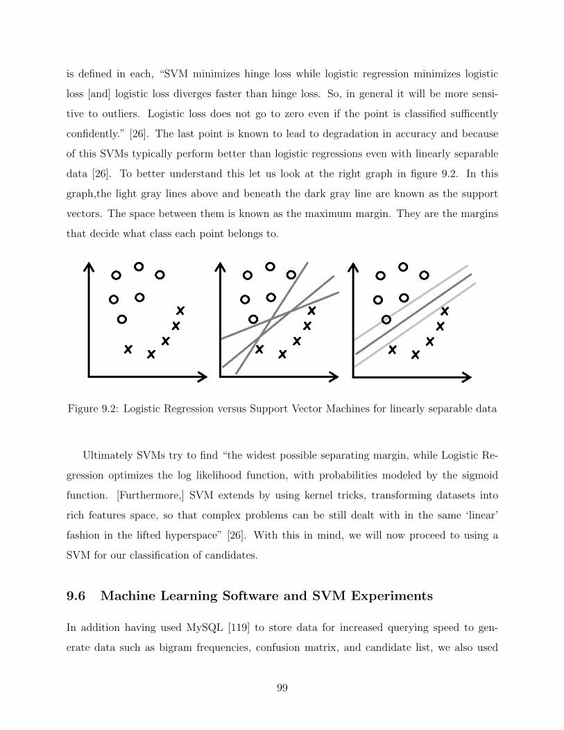
is defined in each, “SVM minimizes hinge loss while logistic regression minimizes logistic
loss [and] logistic loss diverges faster than hinge loss. So, in general it will be more sensi-
tive to outliers. Logistic loss does not go to zero even if the point is classified sufficently
confidently.” [26]. The last point is known to lead to degradation in accuracy and because
of this SVMs typically perform better than logistic regressions even with linearly separable
data [26]. To better understand this let us look at the right graph in figure 9.2. In this
graph,the light gray lines above and beneath the dark gray line are known as the support
vectors. The space between them is known as the maximum margin. They are the margins
that decide what class each point belongs to.
Figure 9.2: Logistic Regression versus Support Vector Machines for linearly separable data
Ultimately SVMs try to find “the widest possible separating margin, while Logistic Re-
gression optimizes the log likelihood function, with probabilities modeled by the sigmoid
function. [Furthermore,] SVM extends by using kernel tricks, transforming datasets into
rich features space, so that complex problems can be still dealt with in the same ‘linear’
fashion in the lifted hyperspace” [26]. With this in mind, we will now proceed to using a
SVM for our classification of candidates.
9.6 Machine Learning Software and SVM Experiments
In addition having used MySQL [119] to store data for increased querying speed to gen-
erate data such as bigram frequencies, confusion matrix, and candidate list, we also used
99

Python [113] versions 2.7 and 3.6.7 to automate the entire system using a bash script in
Ubuntu 16 and 18 virtual machines.
To run the Machine Learning Algorithms we used several software for different tasks.
Most importantly to run the SVM we used LIBSVM – A Library for Support Vector Machines
by Chih-Chung Chang and Chih-Jen Lin [15].
LIBSVM is an integrated software for support vector classification, (C-SVC, nu-SVC),
regression (epsilon-SVR, nu-SVR) and distribution estimation (one-class SVM). It supports
multi-class classification [15]. It is available in many different programming languages in-
cluding the version we used in Python. The main available options and features are:
options:
-s svm_type : set type of SVM (default 0)
0 -- C-SVC
1 -- nu-SVC
2 -- one-class SVM
3 -- epsilon-SVR
4 -- nu-SVR
-t kernel_type : set type of kernel function (default 2)
0 -- linear: u’*v
1 -- polynomial: (gamma*u’*v + coef0)^degree
2 -- radial basis function: exp(-gamma*|u-v|^2)
3 -- sigmoid: tanh(gamma*u’*v + coef0)
-d degree : set degree in kernel function (default 3)
-g gamma : set gamma in kernel function (default 1/num_features)
-r coef0 : set coef0 in kernel function (default 0)
-c cost : set the parameter C of C-SVC, epsilon-SVR, and nu-SVR
(default 1)
-n nu : set the parameter nu of nu-SVC, one-class SVM, and nu-SVR
(default 0.5)
-p epsilon : set the epsilon in loss function of epsilon-SVR (default 0.1)
-m cachesize : set cache memory size in MB (default 100)
100

-e epsilon : set tolerance of termination criterion (default 0.001)
-h shrinking : whether to use the shrinking heuristics, 0 or 1 (default 1)
-b probability_estimates : whether to train a SVC or SVR model for
probability estimates, 0 or 1 (default 0)
-wi weight: set the parameter C of class i to weight*C, for C-SVC
(default 1)
Since we are using the following polynomial kernel (u′v + 1)3, then we set the following
options:
param = svm_parameter(’-s 0 -c 10 -t 1 -g 1 -r 1 -d 3’)
"Classify a binary data with polynomial kernel (u’v+1)^3 and C = 10"
If we wanted to run a linear kernel for comparison, we would set:
param = svm_parameter(’-s 0 -t 0 -h 0’)
"Linear binary classification C-SVC SVM"
Now we are ready to begin the experiments. First we try a linear kernel, which should
give us similar results to the Logistic Regression. We run Experiment 1:
EXP1: param = svm_parameter(’-s 0 -t 0 -h 0’)
"Linear binary classification C-SVC SVM"
-Ran on Full DataSet
-First 60% Train, 40% Test
-Achieved 5912/130219 classifications correctly
-That’s a 4.54% accuracy. BAD!
-Time: 11881.338190078735 seconds (3.30 hours)
This is a summary of the output that LIBSVM gives us (svmTERMINALoutput.txt):
101

EXP1:
optimization finished, #iter = 19532800
nu = 0.031871
obj = -6224.740650, rho = 1.270315
nSV = 8306, nBSV = 6072
Total nSV = 8306
Accuracy = 4.54004% (5912/130219) (classification)
Time: 11881.338190078735 seconds
To understand what each line above means we look at the LIBSVM’s Website FAQ
(https://www.csie.ntu.edu.tw/ cjlin/libsvm/faq.html).
• iter is the iterations performed.
• obj is the optimal objective value of the dual SVM problem.
• rho is the bias term in the decision function sgn(wTx− rho).
• nSV and nBSV are number of support vectors and bounded support vectors (i.e.,
αi = C).
• nu-svm is a somewhat equivalent form of C-SVM where C is replaced by nu.
• nu simply shows the corresponding parameter.
More details can be found in the libsvm document [15].
As we can see the low 4.54% accuracy matches what we achieved with the logistic re-
gression. While we ran it with a 60% train and 40% test data set split. We also see similar
results using the previous 80% train and 20% test data split.
The above data among with all the experiments ran is located in the Results folder.
Each experiment is contained under the matching experiment folder. For example, the
above experiment is found in folder EXP1. Each folder includes some of the following files:
102

• svmTERMINALoutput.txt : This file contains the output from LIBSVM. An example
is shown above. In addition to this it als contains all the p label, p acc, and p val
data in raw format. The p label is what the SVM model predicts for a specific data
point used in testing the model. In later experiments additional data such as precision,
recall, f score, and a confusion matrix of True Positive, True Negative, False Positive,
and False Negative is included. Every experiment has this file.
• svmoutput.txt : This is a file that either provides another copy of the p label, p acc,
and p val data, or in later experiments shows a two-column table showing expected
output y and predicted output y for further error analysis.
• libsvm.model : For later experiments this file contains the SVM model that can be
used to predict more data. The model can be loaded and saved using the commands
model = svm load model(‘libsvm.model’) and svm save model(‘libsvm.model’,
model) respectively.
• svmanalysis1.txt and svmanalysis2.txt : These are included for Experiment 12
(EXP12) but can be run and generated for any other experiment using the Python
script trec5svmSMOTE.py. This same version can generate all of the above files as
well for any experiment ran with it. svmanalysis1.txt contains all of the False Posi-
tive and False Negative predictions along with all of the features and correct output.
Similarly, svmanalysis2.txt contains all True Positive and True Negative predictions
along with all features and the correct output. These can then be used for careful error
analysis on where the learning algorithm made mistakes in order to improve it.
For further details and instructions on how to run and replicate each and all, exper-
iment, or run new ones, please see QuickStart.txt. In this file one can see how to
modify parameters such as training to test ratios, input files, and SVM specific parame-
ters such as kernel type. Because of how long the learning algorithms take to run, use
input file test regression matrix.txt, which contains only 9 data points compared to
regression matrix.txt with 325,547 individual data points, for a quick test to make sure
everything is working correctly before running on large datasets.
103

9.7 SVM Results with Polynomial Kernels
Finally, we will run an experiment with a polynomial kernel. To do this we will run
trec5svm.py and use as input the regression matrix.txt file with our features and out-
put.
RegressionTREC5/libsvm-3.23/python\$ python3 trec5svm.py
> svmTERMINALoutput.txt
First we run the SVM model with a polynomial kernel on our training data as we did
before.
EXP4: param = svm_parameter(’-s 0 -c 10 -t 1 -g 1 -r 1 -d 3’)
"Classify a binary data with polynomial kernel (u’v+1)^3 and C = 10"
-Ran on Full DataSet
-100% Train, 100% Test (so same data we train we test with)
-Achieved 313475/325547 classifications correctly
-That’s a 96.2918% accuracy. GOOD!
-Time: 26164.813225507736 seconds (7.27 hours)
This is a summary of the output that LIBSVM gives us (svmTERMINALoutput.txt):
EXP4:
optimization finished, #iter = 32554700
nu = 0.050608
obj = -1531685219869132324864.000000, rho = -60738085076395.093750
nSV = 16578, nBSV = 16395
Total nSV = 16578
Accuracy = 96.2918% (313475/325547) (classification)
Time: 26164.813225507736 seconds
104

After about 32.5 million iterations and several hours, the model achieves a 96.29% ac-
curacy. This is statistically significant compared to the 92.78% achieved by the logistic
regression; however this is just training data and the real test comes when we run it on the
test data. To see how well it generalized.
Therefore, we run with a 80% Train and 20% Test distribution using the same SVM
model parameters and polynomial kernel:
EXP8: param = svm_parameter(’-s 0 -c 10 -t 1 -g 1 -r 1 -d 3’)
"Classify a binary data with polynomial kernel (u’v+1)^3 and C = 10"
"Re-run of EXP2, but with Precision and Recall output"
-Ran on Full DataSet
-First 80% Train, 20% Test
-Achieved 60958/65110 classifications correctly
-That’s a 93.6231% accuracy. GOOD!
-Precision: 85.32%
-Recall: 10.83%
-F-Score: 0.1922
-Time: 18892.750891447067 seconds (5.25 hours)
This is a summary of the output that LIBSVM gives us (svmTERMINALoutput.txt):
EXP8:
optimization finished, #iter = 26043700
nu = 0.044441
obj = -1033776563990009085952.000000, rho = -1896287955440235.250000
nSV = 11840, nBSV = 11439
Total nSV = 11840
Accuracy = 93.6231% (60958/65110) (classification)
Metrics:
105

Total Instances: 65110
True Positive: 494
False Positive: 85
False Negative: 4067
True Negative: 60464
Confusion Matrix:
__________________
| 494 | 85 |
|_______|________|
| 4067 | 60464 |
|_______|________|
Precision: 85.31951640759931%
Recall: 10.830958123218593%
Accuracy: 93.62309937029643%
F-Score: 0.19221789883268484
End Metrics
Writing Output/Predicted Classes to svmoutput.txt
All Done.
Time: 18892.750891447067 seconds
After about 26 million iterations and 5.25 hours, the model achieves a victorious 93.62%
accuracy on the test data. This may not be as high as the 96.29% accuracy on the training
data, but that is to be expected as the model has never seen the test data. This is a great
indication that there is very little, if any, overfitting in our model and that it has generalized
106

successfully.
Note that we ran additional experiments (EXP3, EXP7) to conclude that the best train-
ing/test ratio was 80% Train and 20% Test. By this we mean that we need at least 260,000
data points to be able to train our algorithm properly. Because the TREC-5 data set is
far larger than this. We will be experimenting on further parts of it with just this small
percentage of the data as training in future tests. Also note that EXP2 is the same as EXP8
without the additional metrics.
At this point we have improved tremendously between the linear kernel and the polyno-
mial kernel based on just accuracy, but does that mean we are done? Not quite...
Accuracy does not tell the full story of the performance of our model for the test data.
This is where Precision, Recall, and F-Score come in to play. These metrics allow us to
better judge how good the learning algorithm is classifying and what the 6.38% error rate
(1 - accuracy = error rate) really means for our task of trying to choose the right candidate
word. But first let us take a look at the four possible outcomes that our learning algorithm
can have:
• True Positive (Output:1 — Predicted: 1) : TP
• False Positive (Output:0 — Predicted: 1) : FP
• False Negative (Output:1 — Predicted: 0) : FN
• True Negative (Output:0 — Predicted: 0) : TN
If Given the five features, the model accepts the candidate word and that word is the
correct word from the aligned ground truth, then that is a True Positive. On the other
hand if the model accepts the candidate word, but that word was not the correct word then
this is known as a False Positive. False positives count as errors and are included in the
error rate.
On the other hand if given the five features, the model rejects the candidate word and
that word was the correct word from the aligned ground truth text, then that word is a
False Negative. This means that the model should have not rejected the word, but it
did. We can think of false negatives as the model not having the confidence to accept the
107
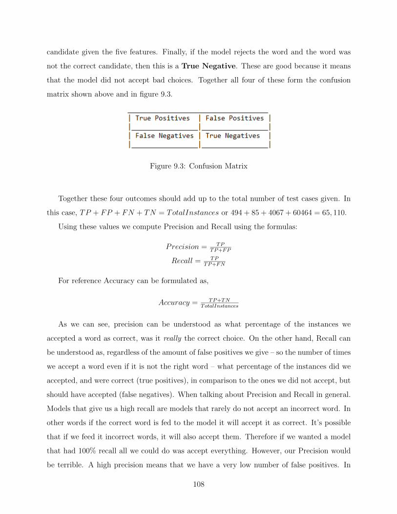
candidate given the five features. Finally, if the model rejects the word and the word was
not the correct candidate, then this is a True Negative. These are good because it means
that the model did not accept bad choices. Together all four of these form the confusion
matrix shown above and in figure 9.3.
Figure 9.3: Confusion Matrix
Together these four outcomes should add up to the total number of test cases given. In
this case, TP + FP + FN + TN = TotalInstances or 494 + 85 + 4067 + 60464 = 65, 110.
Using these values we compute Precision and Recall using the formulas:
Precision = TPTP+FP
Recall = TPTP+FN
For reference Accuracy can be formulated as,
Accuracy = TP+TNTotalInstances
As we can see, precision can be understood as what percentage of the instances we
accepted a word as correct, was it really the correct choice. On the other hand, Recall can
be understood as, regardless of the amount of false positives we give – so the number of times
we accept a word even if it is not the right word – what percentage of the instances did we
accepted, and were correct (true positives), in comparison to the ones we did not accept, but
should have accepted (false negatives). When talking about Precision and Recall in general.
Models that give us a high recall are models that rarely do not accept an incorrect word. In
other words if the correct word is fed to the model it will accept it as correct. It’s possible
that if we feed it incorrect words, it will also accept them. Therefore if we wanted a model
that had 100% recall all we could do was accept everything. However, our Precision would
be terrible. A high precision means that we have a very low number of false positives. In
108

other words we do not accept words that are incorrect. We could have a very high precision
and low recall model meaning that we are very selective and only accept candidates that
we are very confident on. However, if doing this we miss borderline cases and have a lot of
correct words we do not accept. Then our recall drops badly. In the perfect world we want
both of these to be 100% meaning there are no false positives or negatives and, therefore,
100% accuracy.
For our problem deciding if we want high recall or high precision model we have to decide
if we want an OCR Post Processing system that will correct a few words without making
mistakes (high precision), but still leave mistakes in the text, or a model that will detect and
correct a lot more mistakes, but will sometimes correct to the wrong choice (high recall).
To decide we must consider if this is the final step of the OCR post processing or if this is
just part of a pipeline of several models this will be fed in. If the latter is the case we can
choose the second variant because this means that while we will suggest incorrect words as
correct, we will also include the correct words so we are narrowing the candidate list and
then leaving it for a model down the pipeline to hopefully make the right choice. This means
that we detect the correct candidate, but also some incorrect and pool them together for
someone else to decide. This is the ideal choice for that system. However, if this is the final
post processing step before the text reaches the end then we want a high precision model
that only chooses correct candidates in order to not introduce harder to detect errors in the
OCR’d text. If a human is reading the text and sees a misspelled word it will know that it
is most likely an OCR generated error and possibly even correct it on the fly if not too hard,
but if the same human sees a correctly spelled word that does not match the original text
then it is possible he will assume it is a mistake of the text and not of the OCR process.
Because of the contrast between Precision and Recall, researchers sometimes prefer a
single value when comparing overall models with others. This is where F-score comes in.
F-score also known as F1-Score is the harmonic mean of precision and recall:
F1− Score = 2 ∗ Precision∗RecallPrecision+Recall
This can also be defined in terms of Type I and II errors,
F1− Score = 2TP2TP+FN+FP
109

There are also many other scoring systems including F-score variations that give differ-
ent weight to precision and recalls (such as F0.5 that weights recall lower than precision).
Ultimately it depends on the problem one is working with to define the benchmark metrics
that better measure how good a model compares to the state of the art.
Coming back to our results, we achieve:
• Precision: 85.32%
• Recall: 10.83%
• Accuracy: 93.62%
• F-Score: 0.1922
So even though our accuracy was high at 93.62% the recall is very low at only 10.83%.
This means there were a lot of false negatives in our test, or instances where the right
candidate was suggested but the model rejected them. 4,067 correct words were rejected
while only 494 candidates were accepted. This of course is not very good. Nevertheless, the
precision was very high at 85.35% with only 85 instances accepted that shouldn’t have been
accepted (false positives). Therefore because we are using the harmonic mean, our F-score
was low at 0.1922. This raises the question, how can we improve upon this result? Among
many options there are three main ones that we will tackle:
• Rescaling our data
• balancing our classes
• attempting different learning algorithms.
While we will attempt in future work other learning algorithms such as deep learning and
stacked models, then try and produce better results using an ensemble learning technique
with all of these, for now we will focus on the first two.
110

9.8 Normalization and Standardization of Data to increase F-
Score
As shown earlier in section 9.3.2, the data set contains the numerical weights for each feature
in the original format. So for line 122 in our regression matrix.txt data set,
1, 918, 215, 16, 1, 1
using the MySQL query:
SELECT * FROM candidates
WHERE
confusionweight = 918
AND unigramfrequency = 215
AND backwardbigramfreq = 16
AND forwardbigramfreq = 1
AND output = 1;
or the MySQL query:
SELECT * FROM candidates LIMIT 121,1;
we can find the original candidates table entry:
15, hegulations, Regulations, 1, 918, 215, 16, 1, 1, -1, FR940104-0-00001
Where each of those values represents:
• location: 15
• fromword: hegulations
• toword: Regulations
• distance: 1
111

• confusionweight: 918
• unigramfrequency: 215
• backwardsbigramfreq: 16
• forwardbigramfreq: 1
• output: 1
• decision: -1
• docsource: FR940104-0-00001
The ones in bold are the ones found in the regression matrix.txt entry.
As we can see, each of these values are all positive and range from 1 (forwardbigramfreq)
to 918 (confusionweight. Analyzing the entire dataset we can see that the range of each
feature is:
• distance: 0 - 3 (Levenshtein Edit Distance, we limited candidates suggest to a maximum
distance of 3, hence we only have 0 to 3.
• confusionweight: 0 - 3,347 (how common that character edit appears)
• unigramfrequency: 1 - 11,172 (how common the word is)
• backwardsbigramfreq: 0 - 1,581 (how common the bigram is)
• forwardbigramfreq: 0 - 1,015 (how common the bigram is)
• output: 0 - 1 (two classes: correct candidate or incorrect candidate)
So overall, all natural numbers are possible and in our case range from 0 to 11,172.
This creates a problem when trying to compute weights for each feature in our logistic
regression and in our Support Vector Machine. Naturally, the high range of values for the
unigram frequency and confusion weight have to compete with the low range of values for
bigram frequencies and the very low range of values for edit distance. Therefore, if we have
112

a regression model that works using x1 ∗w1 +x2 ∗w2 +x3 ∗w3 +x4 ∗w4 +x5 ∗w5 = y where xi
are the input features and wi are the computed weights. It will be very difficult to converge
a model that uses very different values for each x.
To solve this problem we can rescale our data set in two popular ways known as Stan-
dardization and Normalization. The idea behind rescaling our data is to shrink the range
that these numbers can be so that each feature can have a similar range and avoid this
problem. It is important to note that even though we are changing the values. We still want
them to maintain their numerical order and significance. So if we have two numbers 10 and
50 and we were to make them 1 and 5 they would maintain their order and never would the
5 go before the 1.
9.8.1 Z-score Standardization
Standardization, also known as Z-score Standardization, of a data set involves taking each
feature and computing the mean (µ) and the standard deviation (σ), hence the name stan-
dardization, and updating each instance of xij in the dataset with the following formula:
xij = xij−µjσj
The main idea of this is to rescale the data set into a Gaussian Distribution with µ = 0
and a variance of 1.
9.8.2 MinMax Normalization
Normalization, also known as MinMax scaling, will rescale the data into a range between 0
and 1 for a positive data set, like ours, or into the range -1 to 1 for a data set that contains
negative values. To do this, one must compute the range of each feature, as we did earlier
and then uses these max(xi) and min(xi) to update each instance of xij in the dataset:
xij = xij−min(xi)max(xi)−min(xi)
One disadvantage to minmax scaling compared to z-score standardization is that min-
max is sensitive to outliers data points. Meaning that if the features have outliers it can
unnecessarily compress the range of the majority of the non-outliers data.
113

Something to note is that both of these methods turned our natural number features into
rational number features represented with decimals to a certain digit. We have lost accuracy
a certain level of accuracy. While it is possible to convert them back to the original values.
Such as keeping the original min and max values used in the case of Min-max scaling, it will
be necessary to round to the nearest natural number to recover the original number.
Scaling methods will affect different learning algorithm’s output. Both logistic regression
and SVMs will benefit greatly along with others like Neural Networks, but some like Random
Forest Trees and Classification and Regression Trees, because of how they work, do not
benefit as much if at all.
9.9 LIBSVM Experiment with MinMax Normalization and Z-
score Standardized Data
Now that we have described our scaling methods we will experiment applying it to
regression matrix.
First we will use trec5standarize.py found in the ModifiedDataSets folder to generate
a Z-score Standardized version of our data set: std regression matrix.txt. We run the
python script:
RegressionTREC5/libsvm-3.23/python/ModifiedDataSets\$
python3 trec5standarize.py
The Terminal output of the program:
Beginning Standardization of Data Set
Quick Test: Should be Close to 0:
2.0056514782318402e-08
325547 Rows Affected
Standardization Complete.
114

Time: 3.236551523208618 seconds
As we can see it was very fast to standardize the all five features of the entire 325,547
data instances. The following is a sample of the first 10 lines of the normal dataset, followed
by the equivalent lines in the standardized dataset:
First 10 lines of regression_matrix.txt
3, 37, 2, 0, 0, 0
1, 918, 83, 83, 0, 1
3, 459, 4, 0, 0, 0
3, 1, 4, 0, 0, 0
1, 8, 1, 0, 0, 0
3, 93, 2, 0, 0, 0
1, 186, 1, 0, 0, 0
1, 1, 78, 0, 0, 0
1, 2, 34, 0, 0, 1
3, 0, 27, 0, 0, 0
Some of the values have been truncated to fit in this page. Original accuracy remains in
std regression matrix.txt:
First 10 lines of std_regression_matrix.txt
0.9000758598, -0.188141199827, -0.2033185211, -0.105911163, -0.069130207, 0
-1.284449916, 2.0659022621880, 0.01263117827, 4.7887509463, -0.069130207, 1
0.9000758598, 0.8915481769838, -0.1979864298, -0.105911163, -0.069130207, 0
0.9000758598, -0.280247402588, -0.1979864298, -0.105911163, -0.069130207, 0
-1.284449916, -0.262337863163, -0.2059845668, -0.105911163, -0.069130207, 0
0.9000758598, -0.044864884421, -0.2033185211, -0.105911163, -0.069130207, 0
-1.284449916, 0.1930761393786, -0.2059845668, -0.105911163, -0.069130207, 0
-1.284449916, -0.280247402588, -0.0006990501, -0.105911163, -0.069130207, 0
115

-1.284449916, -0.277688896956, -0.1180050596, -0.105911163, -0.069130207, 1
0.9000758598, -0.282805908221, -0.1366673793, -0.105911163, -0.069130207, 0
Note that we did not standardize or modify the last value of each line since that is
the output class for each candidate that we use to train and test the model. Note that
values that contained the same number within the same column, but in different rows, have
the same value after Standardization. For example, rows 3 and 4 had the value 4 for the
unigram frequency and now have -0.19798642975159997. However, the unigram frequency
and backwards bigram frequency were both 83 for in second row. After the standardization
they have different values: (0.012631178269316813 and 4.788750946292023). This is what we
are after when standardizing and normalizing values as we do not want the actual numbers
to bias or make one column more important than the other before even feeding it to the
learning algorithm.
Next, we will use trec5normalize.py, also found in the ModifiedDataSets folder, to
generate a normalized version of the dataset using MinMax scaling. This file will be saved
in the same directory under the name: norm regression matrix.txt.
We run the python script:
RegressionTREC5/libsvm-3.23/python/ModifiedDataSets\$
python3 trec5normalize.py
The Terminal output of the program:
Beginning Normalization of Data Set
Mins: [0, 0, 1, 0, 0, 0]
Maxs: [3, 3347, 11172, 1581, 1015, 1]
325547 Rows Affected
Normalization Complete.
116
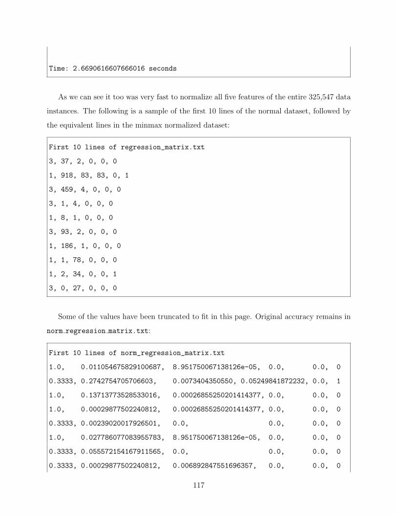
Time: 2.6690616607666016 seconds
As we can see it too was very fast to normalize all five features of the entire 325,547 data
instances. The following is a sample of the first 10 lines of the normal dataset, followed by
the equivalent lines in the minmax normalized dataset:
First 10 lines of regression_matrix.txt
3, 37, 2, 0, 0, 0
1, 918, 83, 83, 0, 1
3, 459, 4, 0, 0, 0
3, 1, 4, 0, 0, 0
1, 8, 1, 0, 0, 0
3, 93, 2, 0, 0, 0
1, 186, 1, 0, 0, 0
1, 1, 78, 0, 0, 0
1, 2, 34, 0, 0, 1
3, 0, 27, 0, 0, 0
Some of the values have been truncated to fit in this page. Original accuracy remains in
norm regression matrix.txt:
First 10 lines of norm_regression_matrix.txt
1.0, 0.011054675829100687, 8.951750067138126e-05, 0.0, 0.0, 0
0.3333, 0.2742754705706603, 0.0073404350550, 0.05249841872232, 0.0, 1
1.0, 0.13713773528533016, 0.00026855250201414377, 0.0, 0.0, 0
1.0, 0.00029877502240812, 0.00026855250201414377, 0.0, 0.0, 0
0.3333, 0.00239020017926501, 0.0, 0.0, 0.0, 0
1.0, 0.027786077083955783, 8.951750067138126e-05, 0.0, 0.0, 0
0.3333, 0.055572154167911565, 0.0, 0.0, 0.0, 0
0.3333, 0.00029877502240812, 0.006892847551696357, 0.0, 0.0, 0
117

0.3333, 0.0005975500448162533, 0.0029540775221555816, 0.0, 0.0, 1
1.0, 0.0, 0.0023274550174559126, 0.0, 0.0, 0
Again we did not modify the output column for the same reason. Note that the first
column contains the values 1.0 and 0.333. This makes sense since the range of that column
can be 0,1,2 or 3 and the equivalent normalized values would be 0.0, 0.333, 0.666 and 1.0
(0.999 repeating is rounded up to 1). Furthermore, just like with Standardization, values
that previously matched in different columns, like 83 in row 2, are again now different. Again,
this is good!
Now that we have generated the normalized and standardized data sets we can re-run
our SVM with polynomial kernel on each of them and compare the results to the original
dataset.
First we run the standardized data set. To do this we will run trec5svm.py and use
as input the standardized dataset: std regression matrix.txt file with our features and
output.
RegressionTREC5/libsvm-3.23/python\$ python3 trec5svm.py
> svmTERMINALoutput.txt
We run with a 80% Train and 20% Test distribution using the same SVM model param-
eters and polynomial kernel:
EXP10: param = svm_parameter(’-s 0 -c 10 -t 1 -g 1 -r 1 -d 3’)
"Classify a binary data with polynomial kernel (u’v+1)^3 and C = 10"
"Re-run of EXP8, but with Standardized dataset"
-Ran on Full DataSet
-First 80% Train, 20% Test
-Achieved 3921/65110 classifications correctly
-That’s a 6.02212% accuracy. BAD!
-Precision: 5.216%
-Recall: 72.31%
118

-F-Score: 0.0973
-Time: 27806.403403520584 seconds (7.72 hours)
This is a summary of the output that LIBSVM gives us (svmTERMINALoutput.txt):
EXP10:
optimization finished, #iter = 26043700
nu = 0.055604
obj = -4198782.413391, rho = -6.952836
nSV = 15120, nBSV = 14020
Total nSV = 15120
Accuracy = 6.02212% (3921/65110) (classification)
Metrics:
Total Instances: 65110
True Positive: 3298
False Positive: 59926
False Negative: 1263
True Negative: 623
Confusion Matrix:
__________________
| 3298 | 59926 |
|_______|________|
| 1263 | 623 |
|_______|________|
Precision: 5.216373529039605%
Recall: 72.30870423152818%
Accuracy: 6.022116418368914%
119

F-Score: 0.09730766393744929
End Metrics
Writing Output/Predicted Classes to svmoutput.txt
All Done.
Time: 27806.403403520584 seconds
After about 26 million iterations and 7.72 hours, the model achieves a terrible 5.216%
accuracy on the test data. This is terrible, but not surprising. Something to note is that
the recall went up to the highest we have seen with 72.31% recall. This means that there
were very few False negatives. However, because of the low precision this can be explained
by the model being too relaxed and accepting everything as we can see by the huge number
of false positives.
Next we run the minmax normalized data set. To do this we will run trec5svm.py and
use as input the normalized dataset: norm regression matrix.txt file with our features
and output.
RegressionTREC5/libsvm-3.23/python\$ python3 trec5svm.py
> svmTERMINALoutput.txt
First we run the SVM model with a polynomial kernel on our training data:
EXP11: param = svm_parameter(’-s 0 -c 10 -t 1 -g 1 -r 1 -d 3’)
"Classify a binary data with polynomial kernel (u’v+1)^3 and C = 10"
"Re-run of EXP4, but with Normalized dataset"
-Ran on Full DataSet
-100% Train, 100% Test (so same data we train we test with)
-Achieved 314623/325547 classifications correctly
120

-That’s a 96.6444% accuracy. GOOD!
-Precision: 72.94%
-Recall: 42.14%
-F-Score: 0.5342
-Time: 603.8748393058777 seconds (10.06 minutes!)
This is a summary of the output that LIBSVM gives us (svmTERMINALoutput.txt):
EXP11:
optimization finished, #iter = 128817
nu = 0.072905
obj = -235549.460276, rho = -1.022669
nSV = 23796, nBSV = 23676
Total nSV = 23796
Accuracy = 96.6444% (314623/325547) (classification)
Metrics:
Total Instances: 325547
True Positive: 6264
False Positive: 2324
False Negative: 8600
True Negative: 308359
Confusion Matrix:
__________________
| 6264 | 2324 |
|_______|________|
| 8600 | 308359 |
|_______|________|
121

Precision: 72.93898462971589%
Recall: 42.142088266953714%
Accuracy: 96.64441693518908%
F-Score: 0.5341975098072659
End Metrics
Writing Output/Predicted Classes to svmoutput.txt
All Done.
Time: 603.8748393058777 seconds
After only 128,817 iterations and a shocking 10 minutes and four seconds the algorithm
has finished. This is a massive improvement over the previous experiment that took multiple
hours. The only difference between this and the previous experiment was normalizing the
dataset with a minmax scaler. Another process that took seconds to complete. This is a
great example of the power of rescaling data. The model achieved a respectable 96.64%
accuracy on the training data, but will it generalize well?
9.9.1 The best LIBSVM Experiment with MinMax Normalization
For the final test we will run the normalized dataset, normalized regression matrix.txt,
with a 80% Train and 20% Test distribution using the same SVM model parameters and
polynomial kernel than the experiment with the original dataset.
RegressionTREC5/libsvm-3.23/python\$ python3 trec5svm.py
> svmTERMINALoutput.txt
Results:
122

EXP9: param = svm_parameter(’-s 0 -c 10 -t 1 -g 1 -r 1 -d 3’)
"Classify a binary data with polynomial kernel (u’v+1)^3 and C = 10"
"Re-run of EXP8, but with Normalized dataset"
-Ran on Full DataSet
-First 80% Train, 20% Test
-Achieved 62977/65110 classifications correctly
-That’s a 96.724% accuracy. GOOD!
-Precision: 91.58%
-Recall: 58.63%
-F-Score: 0.7149
-Time: 393.0401563644409 seconds (6.55 minutes!)
This is a summary of the output that LIBSVM gives us (svmTERMINALoutput.txt):
EXP9:
optimization finished, #iter = 130782
nu = 0.074323
obj = -192342.464438, rho = -1.000211
nSV = 19409, nBSV = 19303
Total nSV = 19409
Accuracy = 96.724% (62977/65110) (classification)
Metrics:
Total Instances: 65110
True Positive: 2674
False Positive: 246
False Negative: 1887
True Negative: 60303
123

Confusion Matrix:
__________________
| 2674 | 246 |
|_______|________|
| 1887 | 60303 |
|_______|________|
Precision: 91.57534246575342%
Recall: 58.62749397062048%
Accuracy: 96.7240055291046%
F-Score: 0.7148776901483759
End Metrics
Writing Output/Predicted Classes to svmoutput.txt
All Done.
Time: 393.0401563644409 seconds
This is the best run yet at 6 minutes and 33 seconds with 130,782 iterations. The model
achieved a victorious 96.72% accuracy on the test data. This is slightly higher than its
performance on the training data. The model definitely generalized successfully. Analyzing
it further, we can see that Precision was at 91% meaning that there was a very low number
of false positives in comparison to the number of true positives. Do note that we still had
more false positives in this run than with the original data set. As previously we only had
85 false positives. However, in the previous version we only accepted 494 candidates that
were correct whereas in this version we accepted 2,674 candidates that were correct. This is
why the precision still went up even though we had more false positives. Recall, also, greatly
increased to 58.62% meaning that the number of false negatives decreased greatly from 4,067
124

to 1,887.
Normalizing the dataset turned out to be a very successful endeavor in increasing our
accuracy from 93.62% to 96.72%, a statistically significant difference, but most importantly
in increasing our recall from 10.83% to 58.63% while maintaining and slightly increasing our
precision from 85.32% to 91.58%. This also means that our F-score increased from 0.1922 to
0.7149. Aside from the small number of false positives that increased, the learning algorithm
clearly performed better, and was trained much faster, thanks to the minmax normalized
dataset. We have now successfully corrected 58.63% of the errors detected in the OCR
post processing stage, but can we do better? For that we turn to the next improvement,
balancing our class distribution in the training data, but before we would like to show one
more experiment using the normalized training data.
9.10 Scikit-Learn Experiment with Normalized Data
While we used LIBSVM directly for all of our SVM experiments. We also ran a single ex-
periment using Scikit-Learn [78] version of the LIBSVM. Scikit-Learn is a library of different
machine learning algorithms for Python among other data mining and data analysis tools.
It is built on NumPy [74, 112], SciPy [53], and matplotlib [48], allows reading files using
pandas [68], and is open source and accessible to everybody.
This version is found in trec5svmV2.py and can be run as:
RegressionTREC5/scikitSVMversion\$ python3 trec5svmV2.py
> scikitSVMoutput.txt
It uses the norm regression.txt found in the same directory. It’s output:
[[3.33333333e-01 2.74275471e-01 7.34043506e-03 5.24984187e-02
0.00000000e+00 1.00000000e+00]
[1.00000000e+00 1.37137735e-01 2.68552502e-04 0.00000000e+00
0.00000000e+00 0.00000000e+00]
[1.00000000e+00 2.98775022e-04 2.68552502e-04 0.00000000e+00
125

0.00000000e+00 0.00000000e+00]
...
[1.00000000e+00 0.00000000e+00 1.03840301e-02 0.00000000e+00
0.00000000e+00 0.00000000e+00]
[1.00000000e+00 0.00000000e+00 2.68552502e-04 0.00000000e+00
0.00000000e+00 0.00000000e+00]
[3.33333333e-01 2.98775022e-04 8.95175007e-05 0.00000000e+00
0.00000000e+00 0.00000000e+00]]
[[3.33333333e-01 2.74275471e-01 7.34043506e-03 5.24984187e-02
0.00000000e+00]
[1.00000000e+00 1.37137735e-01 2.68552502e-04 0.00000000e+00
0.00000000e+00]
[1.00000000e+00 2.98775022e-04 2.68552502e-04 0.00000000e+00
0.00000000e+00]
...
[1.00000000e+00 0.00000000e+00 1.03840301e-02 0.00000000e+00
0.00000000e+00]
[1.00000000e+00 0.00000000e+00 2.68552502e-04 0.00000000e+00
0.00000000e+00]
[3.33333333e-01 2.98775022e-04 8.95175007e-05 0.00000000e+00
0.00000000e+00]]
[1. 0. 0. ... 0. 0. 0.]
Classification report for SVC(C=10.0, cache_size=8000, class_weight=None,
coef0=1, decision_function_shape=’ovr’, degree=3, gamma=1.0,
126

kernel=’poly’, max_iter=-1, probability=False, random_state=None,
shrinking=True, tol=0.001, verbose=False)
precision recall f1-score support
0.0 0.97 0.99 0.98 62137
1.0 0.73 0.42 0.54 2973
micro avg 0.97 0.97 0.97 65110
macro avg 0.85 0.71 0.76 65110
weighted avg 0.96 0.97 0.96 65110
Confusion matrix
[[61680 457]
[ 1720 1253]]
(’Time:’, 616.8139779567719, ’seconds’)
Note that support is the number of instances of each class in the test data. While
these values are not as good as the LIBSVM version, they are still decent and show a
good point on how choosing the right settings for a model can make a large difference.
Furthermore, many casual users are more familiar using Scikit-learn instead of LIBSVM
directly, and we wanted to provide a model along with code and instructions for users more
comfortable in those settings to follow along and be able to reproduce the experiments with
the tools and environment they are familiar with. Do note that while we developed our own
Normalization and Standardization tools on python, Scikit-learn provides StandardScaler
and MinMaxScaler for Standardization and Normalization respectively.
127

9.11 Over-sampling and Under-sampling
The concept behind balancing our class distribution in our training data is simple. We want
to have an even amount of training instances for each class so that our learning algorithm
does not take a bias. The current distribution of our classes can be quickly checked with a
set of queries:
SELECT count(*) FROM candidates WHERE output = 1; -- 14,864
SELECT count(*) FROM candidates WHERE output = 0; -- 310,683
SELECT count(*) FROM candidates; -- 325,547
SELECT count(*) FROM candidates WHERE output != 1 and output != 0; -- 0
As we can see only 4.566% of the data instances belong to class 1. Ideally we want there to
be an even distribution of test instances to better train the model. The main reason for this
is because every candidate word has only 1 correct choice, but our dictionary generates any
candidate with an edit distance of 3 or less. Therefore most errors will have a high number
of candidates per error. On average that is just under 22 candidates per error. Therefore we
have two options: To either remove class 0 instances (so remove incorrect candidates from
training) or add correct candidates to the training). If we remove incorrect candidates we
would have to leave 1 incorrect suggestion per word along with its correct suggestion. As
for the other option we would need to pull more data from the TREC-5 dataset to have
325,000 errors, and even then we would still only be able to have 1 error candidate per word
along with the correct choice. But what if we want to use the data we have to fix this
problem without removing or adding new instances (suppose we didn’t have more data). We
can use over-sampling. Over-sampling will generate new instances of a certain class using
the previous data by slightly altering the features of existing examples of the class we want
to over-sample. These slightly altered examples become the new data instances. The idea
is that new data that we could run into will probably be not too different from the data
instances we have. This assumption can be dangerous as there needs to be enough data
to over-sample in the first place. if we had only 5 instances of a class, we may not have
enough coverage of how the features of a class really behave and over-sampling can only get
128
us so far. On the other hand if we wished to balance the classes by reducing the class with
more instances we can do that by under-sampling a class. This is far easier as it involves
just removing data instances from the over represented class. However, nothing is easy.
Randomly removing instances will work but ideally we want to first remove instances that
are duplicates or very close to being duplicates of existing data instances. For example, if we
had 10 instances and we were reducing it to 7 but there were 2 duplicates and one two very
unique instances and instead of removing the duplicates we removed the unique instances
we would be hurting the algorithms chances of training successfully and generalizing well.
Typically one will see over-sampling more than under-sampling as the only time it may prove
beneficial is if time is of concern when training a model. It can be useful for creating test
data sets to do quick experiments that are closer to what the real experiments will be like.
One final note is that it is very important to only over-sample or under-sample on the
training data. This way no information will bleed from the test data into the training model
and affect how the model generalizes on a validation set.
9.11.1 Over-sampling techniques
There are many methods to over-sample and under represented class. The simplest method
involves taking random data instances of the under represented class and slightly tweaking
them by a small random factor to create synthetic/artificial samples. We do not want to just
create copies. Do this enough times until the augmented data set has the same amount of
data instances for each class. Doing this will prevent the majority class from “taking over the
other classes during the training process” [60,61]. A better method involves generating new
instances by interpolation. Two popular methods are the Synthetic Minority Over-sampling
Technique (SMOTE) [16], and the Adaptive synthetic sampling approach for imbalanced
learning (ADASYN) [41].
“ADASYN focuses on generating samples next to the original samples which
are wrongly classified using a k-Nearest Neighbors classifier while the basic im-
plementation of SMOTE will not make any distinction between easy and hard
samples to be classified using the nearest neighbors rule. Therefore, the decision
129

function found during training will be different among the algorithms [60,61].”
Imbalanced-Learn has a great library that is now part of Scikit-learn [78] with many over-
sampling techniques including SMOTE and ADASYN [61]. There are also under-sampling
techniques like Tomek-link [24] as well. For more details on different types of over-sampling
along with visual (graph) examples of each over-sampling technique and its results please
visit the official Imbalance-Learn Docs >> User Guide >> Over-sampling [60].
Do note that while SMOTE tends to improve precision and recall due to the balancing of
classes, there are some times where it may not be as effective as random sampling, “SMOTE
does not attenuate the bias towards the classification in the majority class for most classifiers,
and it is less effective than random undersampling. SMOTE is beneficial for k-NN classifiers
based on the Euclidean distance if the number of variables is reduced performing some type
of variable selection and the benefit is larger if more neighbors are used” [63]. Nevertheless,
imbalanced learning continues to be popular in many fields including applications of machine
learning in cancer research [10].
9.12 Over-sampling with SMOTE
Next we will use SMOTE [16]’s implementation in Imbalance Learn’s [61] library in Scikit-
learnscikit-learn to balance our classes and try and improve our precission and recall. We
will also use pandas [68] to read in a modified version of our normalized dataset into a
NumPy [74,112] array that we can then feed to the SMOTE algorithm.
If one wishes to test SMOTE with the test data set, test regression matrix.txt, do
note that it will not work with the SMOTE generator because it is too small. Because of
the way the algorithm works with the k-Nearest neighbor classifier, it is necessary to have
approximately at least 300 or more data points for it to work. This won’t be a problem with
norm regression matrix.txt as, even though we have a big unbalance, we have more than
enough data instances of correct candidates to use SMOTE.
The implementation of SMOTE used can be found in trec5smote.py and can be run as:
RegressionTREC5/libsvm-3.23/python/ModifiedDataSets\$ python3 trec5smote.py
130

It uses as input the normalized data set, norm regression.txt, found in the same
directory and will generate three files as output found in the SMOTE directory inside of
ModifiedDataSets. The three files are:
• smoteTrain regression matrix.txt 80% of the normalized dataset with SMOTE
applied to it.
• regTest regression matrix.txt 80% of the normalized dataset. Unmodified.
• regTrain regression matrix.txt The last 20% of the normalized dataset. Unmod-
ified.
To further understand what each of these files mean here is the output when we run
trec5smote.py.
Creating Train and Test files: regTrain and regTest.
Also creating temporary file: smoteTempTrain
Total Size: 325547
Train Size: 260438
Test Size: 65109
Train Range: 0-260437
Test Range: 260438-325546
Beginning SMOTE Process
Sample:
distance confWeight uniFreq bkwdFreq fwdFreq output
0 1.000000 0.011055 0.000090 0.000000 0.0 0.0
1 0.333333 0.274275 0.007340 0.052498 0.0 1.0
2 1.000000 0.137138 0.000269 0.000000 0.0 0.0
3 1.000000 0.000299 0.000269 0.000000 0.0 0.0
4 0.333333 0.002390 0.000000 0.000000 0.0 0.0
131

Class Distribution Before SMOTE:
0: 250135
1: 10303
Class Distribution After SMOTE:
0: 250135
1: 250135
New Size: 500270
SMOTE Complete.
Removed Temporary File: smoteTempTrain
Finished Writing smoteTrain.
All Done.
Time: 9.28753995895 seconds
As one can see the first step the python script does is separate the dataset into train and
test data and save them as two separate files without any changes(regTrain and regTest).
This is done so we can later compare the performance of SMOTE to the previous version
with the exact same train and test sets. Furthermore, we have to separate the test set before
applying smote in order to not bleed data from the test set into the training set as this will
improve our test set results but will not generalize well and perform poorly in any proper
applications or in a validation set.
After the regular versions are split and saved, we can see that the class distribution is
250,135 data instances belonging to class 0 (incorrect candidates) and 10,303 data instances
belonging to class 1 (correct candidates). This means that class 1 represents only 3.95%
of all data instances. After we run SMOTE we can see that class 0 still has the 250,135
132

instances but class 1 also has 250,135 instances. Meaning that the class distribution is
perfectly balanced, as all things should be... The new size of the training set is almost twice
as big at 500,270. However, because we still split our train and test at 80% Train and 20%
Test, and because these are synthetic instances, we still consider to have that same ratio
even though the training data instances nearly doubled.
We are now ready to test and see what improvements SMOTE has achieved in our SVM.
9.13 Experimenting with SMOTE and LIBSVM
We have modified and created a new version of our SVM Python Script: trec5svmSMOTE.py.
This version takes two files instead of one. A training file and a test file. In addition to
providing all of the previous metrics it will also generate two additional files for error analysis
in the SMOTE directory: svmanalysis1.txt and svmanalysis2.txt. The SVM algorithm
still uses the same polynomial kernel.
We will run three experiments with the new smote data set in a new modified version of
our SVM that takes multiple files):
The first experiment will be using the regTrain regression matrix.txt to train and
regTest regression matrix.txt to test the SVM as a baseline to ensure we achieve the
same results as EXP9.
The second experiment will be using only smoteTrain regression matrix.txt to both
train and test the SVM with SMOTE in order to have a baseline of what our training
accuracy is.
The third, and final, experiment will be using smoteTrain regression matrix.txt to
train the SVM with SMOTE and regTest regression matrix.txt to test the SVM. This
will the key experiment to see if we have an improvement.
Each experiment is run with the same file but modifying the input files in the script.
RegressionTREC5/libsvm-3.23/python\$ python3 trec5svmSMOTE.py
> svmTERMINALoutput.txt
Without further ado we start with the first experiment:
133

9.13.1 Experiment 1: regTrain and regTest
EXP12: param = svm_parameter(’-s 0 -c 10 -t 1 -g 1 -r 1 -d 3’)
"Classify a binary data with polynomial kernel (u’v+1)^3 and C = 10"
"Re-run of EXP9, but using trec5svmSMOTE.py, should give us same as EXP9"
-Ran on Full DataSet but using the split datasets we made
-First 80% Train, 20% Test
-Achieved 62976/65109 classifications correctly
-That’s a 96.724% accuracy. GOOD!
-Precision: 91.58%
-Recall: 58.63%
-F-Score: 0.7149
-Time: 607.9417464733124 second (10.13 minutes!)
This is a summary of the output that LIBSVM gives us (svmTERMINALoutput.txt):
EXP12:
optimization finished, #iter = 129762
nu = 0.074324
obj = -192342.438654, rho = -1.000332
nSV = 19405, nBSV = 19303
Total nSV = 19405
Accuracy = 96.724% (62976/65109) (classification)
Writing Error Analysis to svmanalysis1.txt (FP/FN) and svmanalysis2.txt (TP/TN)
Metrics:
Total Instances: 65109
True Positive: 2674
False Positive: 246
134

False Negative: 1887
True Negative: 60302
Confusion Matrix:
__________________
| 2674 | 246 |
|_______|________|
| 1887 | 60302 |
|_______|________|
Precision: 91.57534246575342%
Recall: 58.62749397062048%
Accuracy: 96.72395521356495%
F-Score: 0.7148776901483759
End Metrics
Writing Output/Predicted Classes to svmoutput.txt
All Done.
Time: 607.9417464733124 second
As expected we achieved the exact same results as our previous experiment with normal-
ized data. This means we can now move on to testing the SMOTE data. It did take over
10 minutes instead of the sub-seven minute run as before but this could be due to external
factors as it took around the same number of iterations.
9.13.2 Experiment 2: smoteTrain only
EXP13: param = svm_parameter(’-s 0 -c 10 -t 1 -g 1 -r 1 -d 3’)
135

"Classify a binary data with polynomial kernel (u’v+1)^3 and C = 10"
"Re-run of EXP9, but with SMOTE applied to the Normalized dataset"
-Ran on Full DataSet but using only the train datasets we made
-100% Train, 100% Test (so same data we train we test with)
-This is a baseline experiment to see how it does on training data alone
-Achieved 439285/500270 classifications correctly
-That’s a 87.8096% accuracy. GOOD.
-Precision: 89.47%
-Recall: 85.71%
-F-Score: 0.8755
-Time: 5255.858581542969 seconds (1.46 hours)
This is a summary of the output that LIBSVM gives us (svmTERMINALoutput.txt):
EXP13:
optimization finished, #iter = 517981
nu = 0.278321
obj = -1369922.733221, rho = -2.488460
nSV = 139339, nBSV = 139145
Total nSV = 139339
Accuracy = 87.8096% (439285/500270) (classification)
Metrics:
Total Instances: 500270
True Positive: 214393
False Positive: 25243
False Negative: 35742
True Negative: 224892
Confusion Matrix:
136

__________________
| 214393| 25243 |
|_______|________|
| 35742 | 224892 |
|_______|________|
Precision: 89.46610692884208%
Recall: 85.71091610530314%
Accuracy: 87.80958282527436%
F-Score: 0.8754826235118045
End Metrics
Writing Output/Predicted Classes to svmoutput.txt
All Done.
Time: 5255.858581542969 seconds
Execution took 1.46 hours and a considerable more amount of iterations than the first
experiment with 517,981 iterations. However this could be due to the larger amount of
training data (even if synthetic) that the algorithm has to process. This is till far less than
the amount it took with the original dataset that was not normalized. The model did not
achieve as high accuracy as before the balancing as it only achieve 87.81% versus 96.72%
without the balancing. However the precision was nearly as high as the previous run, and the
recall was the highest we have seen so far at 85.71% therefore creating the highest F-score
we have seen at 0.8755. However this is just testing on the train data. How will the model
generalize? We will find out in the last experiment.
137

9.13.3 Experiment 3: smoteTrain and regTest
EXP14: param = svm_parameter(’-s 0 -c 10 -t 1 -g 1 -r 1 -d 3’)
"Classify a binary data with polynomial kernel (u’v+1)^3 and C = 10"
"Re-run of EXP9, but with SMOTE applied to the Normalized dataset"
-Ran on Full DataSet but using the split datasets we made.
-Only training DataSet has SMOTE applied to it to avoid biasing test set.
-First 80% Train, 20% Test
-Achieved 59449/65109 classifications correctly
-That’s a 91.3069% accuracy. GOOD.
-Precision: 44.20%
-Recall: 91.89%
-F-Score: 0.5969
-Time: 4078.6771759986877 seconds (67.98 minutes!)
This is a summary of the output that LIBSVM gives us (svmTERMINALoutput.txt):
EXP14:
optimization finished, #iter = 517981
nu = 0.278321
obj = -1369922.733221, rho = -2.488460
nSV = 139339, nBSV = 139145
Total nSV = 139339
Accuracy = 91.3069% (59449/65109) (classification)
Metrics:
Total Instances: 65109
True Positive: 4191
False Positive: 5290
False Negative: 370
138

True Negative: 55258
Confusion Matrix:
__________________
| 4191 | 5290 |
|_______|________|
| 370 | 55258 |
|_______|________|
Precision: 44.204197869423055%
Recall: 91.88774391580795%
Accuracy: 91.30688537682963%
F-Score: 0.5969235151687794
End Metrics
Writing Output/Predicted Classes to svmoutput.txt
All Done.
Time: 4078.6771759986877 seconds
Interestingly enough the model performed better in terms of accuracy on the test data
than it did on the training data with a 91.30% accuracy versus the training data’s 87.81%
accuracy. Both however are short of the 96.72% accuracy of first experiment with the
imbalanced normalized data set. In terms of precision we had a low precision of 44.20%
meaning the model did not generalize well in terms of precision meaning that we had a
higher amount of false positives than before. However, we surprisingly achieved the highest
recall we have seen, even surpassing the training set with a recall of 91.89% compared to
the training set’s 85.71% and the imbalanced model’s recall of 58.63%. These means we
139

have very few false negatives. It is very clear that SMOTE balancing the classes greatly
improved the recall at the cost of the precision. An interesting trade of. This resulted in
an F-Score of 0.5969 compared to the imbalance model’s 0.7149 F-score. In more careful
analysis we can see that the model seems to choose as many correct candidates as it does
incorrect candidates. All in all while we had a very high recall, the trade off loss in precision
makes SMOTE not the clear winner. It appears that the normalized imbalance dataset was
the best result, so far.
9.14 Discussion and Error Analysis
Given the varying results with the SMOTE dataset it appears an ensemble learning technique
could help combine both models into one that maintains a high recall without so much preci-
sion loss. Further exploration of this approach will be done in the near future. Furthermore,
there are many other class balancing algorithms to experiment with including variations of
SMOTE, ADASYN [41] and also, under sampling techniques like TOME-LINK [24] that are
worth exploring.
In addition to that we can analyze the errors that the learning algorithm is making to
try and add features or help us in modifying hyper parameters to improve the model. To do
this we will look at the two files we generated with the last set of experiments:
• svmanalysis1.txt contains a list of all misclassification by first listing all False Posi-
tives, followed by some empty lines, and then followed by a list of all False Negatives.
• svmanalysis2.txt contains a list of all correct classifications by first listing all True
Positives, followed by some empty lines, and then followed by a list of all True Nega-
tives.
Because we are interested in finding out what was misclassified by our model, we will
focus on svmanalysis1.txt, but we welcome readers to do further analysis on this files for
their own research.
Here is a sample of the file (some values were truncated. See original file for full accuracy):
140

Index distance confWeight uniFreq bkwdFreq fwdFreq Output Predicted
1247 0.666667 0.50014939 0.001969385 0.0 0.004926108 0.0 1.0
1464 0.666667 0.50014939 0.001342763 0.0006325 0.003940887 0.0 1.0
2082 0.666667 0.49985061 8.95175e-05 0.0 0.000985222 0.0 1.0
2342 0.666667 0.50044816 0.0 0.0 0.0 0.0 1.0
3113 0.666667 0.50642366 0.0 0.0 0.0 0.0 1.0
...
54 0.666667 0.17747236 0.000805658 0.0006325 0.0 1.0 0.0
113 1.0 0.00029878 0.0 0.0 0.000985222 1.0 0.0
131 0.333333 0.27427547 0.002775043 0.0018975 0.001970443 1.0 0.0
197 0.333333 0.18524051 0.004565393 0.0006325 0.001970443 1.0 0.0
223 0.333333 0.27427547 8.95175e-05 0.0012650 0.001970443 1.0 0.0
The first five lines show the first five false positives we encounter and the last five lines
show the first five false negatives that we encountered. The index represents the data instance
in relation to the specific data set. In this case the test data set. So we will have to do some
shifting to locate the entry in the candidates table. Furthermore, in order to identify which
candidates these were we must convert the normalized data back to the original data set.
We can do that by reversing the minmax scaler formula from:
yij = xij−min(xi)max(xi)−min(xi)
To:
xij = min(xi) + yij ∗ (max(xi)−min(xi)
where yij is our normalized value and xij is our original value.
Using this formula we can try to identify the first line of the above svmanalysis1.txt
by converting the normalized value of the unigram frequency: 0.00196938501477 back to its
original value of 23. We can also directly locate the line in the candidates table by taking the
index and adding it to the product of the candidates table size (325,547) times 0.8 (80%) this
141

will give us the original index. In this case, 261,684. We can then query it in the candidates
table using LIMIT to offset 261,684 lines:
-- 1) False Positive Example:
SELECT 1+( 0.00196938501477 )*(11172-1); -- 23
SELECT (325547*0.8) + 1247 ; -- 261684
SELECT * FROM candidates LIMIT 261684, 8;
-- Found in second row 23 unigram freq. Matched!
As we can see, the above query returns us the original candidates table entry located in
the second row:
116529, prodects1, products, 2, 222, 158, 0, 7, 0, -1, FR940104-0-00043
116529, prodects1, products,, 2, 1674, 23, 0, 5, 0, -1, FR940104-0-00043
116529, prodects1, products., 2, 30, 28, 0, 0, 0, -1, FR940104-0-00043
116529, prodects1, projected, 3, 120, 7, 0, 0, 0, -1, FR940104-0-00043
116529, prodects1, projects, 2, 342, 7, 0, 2, 0, -1, FR940104-0-00043
116529, prodects1, projects,, 2, 1793, 1, 1, 1, 1, -1, FR940104-0-00043
116529, prodects1, Projects., 3, 100, 3, 0, 0, 0, -1, FR940104-0-00043
116529, prodects1, protect, 3, 39, 18, 0, 1, 0, -1, FR940104-0-00043
Reminder: Columns in order from left to right are location, fromword, toword, distance,
confusionweight, unigramfrequency, backwardbigramfreq, forwardbigramfreq, output, deci-
sion, and docsource.
From this we can see that the error word ‘prodects1’ was predicted as ‘products’ by
the model, but the correct candidate should have been ‘projects,’ The confusion weights
were similar for both candidates, 1674 and 1793 respectively, but ‘products’, had a higher
unigram frequency of 23 versus 1 for ‘projects,’. ‘products’, also had a higher forward
bigram frequency, 5 versus 1, than ‘projects,’. However, ‘projects,’ did have one instance of
a backwards bigram versus a 0 frequency for ‘products’.
142

Ultimately both are very similar and context is absolutely necessary to see which one is
correct. To do this we can identify the surrounding 6-gram phrase from both the OCR’d
Text and the Original text thanks to the alignment algorithm:
Query:
SELECT * FROM doctext WHERE location >= 116527 LIMIT 6;
-- 6-gram OCR’d Text
Output:
word: location: locationOR: docsource:
bany, 116527, 114963, FR940104-0-00043
protection, 116528, 114964, FR940104-0-00043
prodects1, 116529, 114965, FR940104-0-00043
and, 116530, 114966, FR940104-0-00043
NMFS, 116531, 114967, FR940104-0-00043
anticipates, 116532, 114968, FR940104-0-00043
Query:
SELECT * FROM doctextORIGINAL WHERE location >= 114963 LIMIT 6;
-- 6-gram Original Text
Output:
word: location: docsource:
bank, 114963, FR940104-0-00043
protection, 114964, FR940104-0-00043
projects,, 114965, FR940104-0-00043
and, 114966, FR940104-0-00043
NMFS, 114967, FR940104-0-00043
anticipates, 114968, FR940104-0-00043
If we look at the 6-gram of both the original text and the OCR’d text we see:
143

Original 6-gram:
bany protection, projects, and NMFS anticipates
OCR’d text 6-gram:
bank protection, prodects1, and NMFS anticipates
That both words ‘projects’ and ‘products’ would fit as correct candidates given the con-
text of the 6-gram. In this sense the algorithm made the human choice to pick the more
common word and hope for the best. It is doubtful a human would know which of the two
to pick with just this information as well. So what could we have done? Do we give up? Of
course not, we could look further than the bigram frequency in our feature set to and try
and see what the document is about in future models. The more context we have, the more
features we have and the better chances of predicting the right word. However, with more
context and more features the bigger the dataset and the slower the training time so at a
certain size the trade off is too high, but further exploration into this will be done in the
future.
Next we can look at the first example of a false negative in svmanalysis1.txt:
54 0.666667 0.17747236 0.000805658 0.0006325 0.0 1.0 0.0
Using this the same for formula we can again convert the normalized value of the unigram
frequency: 0.000805657506042 back to its original value of 10. We can also directly locate
the line in the candidates table by taking the index and adding it to the product of the
candidates table size as we did before.
-- 2) False Negative Example:
SELECT 1+( 0.000805657506042 )*(11172-1); -- 10
SELECT (325547*0.8) + 54 ; -- 260491
SELECT * FROM candidates LIMIT 260491, 8;
-- Found in second row 10 unigram freq. Matched!
144

As we can see, the above query returns us the original candidates table entry located in
the second row:
115768, sprlng, spread, 3, 0, 2, 0, 0, 0, -1, FR940104-0-00042
115768, sprlng, Spring, 2, 594, 10, 1, 0, 1, -1, FR940104-0-00042
115768, sprlng, Spring,, 3, 458, 1, 0, 0, 0, -1, FR940104-0-00042
115768, sprlng, string), 3, 399, 1, 0, 0, 0, -1, FR940104-0-00042
115768, sprlng, strong, 2, 29, 5, 0, 0, 0, -1, FR940104-0-00042
115768, sprlng, wrong, 3, 29, 3, 0, 0, 0, -1, FR940104-0-00042
115769, creey, agree, 3, 73, 22, 0, 0, 0, -1, FR940104-0-00042
115769, creey, came, 3, 1, 1, 0, 0, 0, -1, FR940104-0-00042
In this case, the suggested candidate word ‘Spring’ was rejected as the correct candidate
for the error word ‘sprlng’. The character ‘l’ was misclassified as an ‘i’ by the OCR scanning
software, a very common mistake. In fact it is such a common mistake that our confusion
matrix ranks it number 4 amongst most common error corrections (l→ i).
Query:
SELECT * FROM confusionmatrix ORDER BY frequency DESC LIMIT 5;
Output:
1, ,, 3347
l, d, 1421
y, k, 1224
l, i, 1188
fl, i, 1164
As we can see the fourth most common edit is (l → i) however the confusion weight for
it (1188) does not match the confusion weight for our candidate entry. The reason for this
is because technically there are two edits happening. The ‘s’ is being capitalized (s → S)
and the l→ i.
145

In future versions we intend to improve on this by lowercasing the entire corpus therefore
eliminating inflated Levenshtein edit distances between the candidate word and error word.
In addition to this, we will be removing all punctuation from candidate words and correct
words. By doing this we will be able to combine entries like ‘Spring’ and ‘Spring’ in order
to make the current features we have more robust.
Next we identify the 5-gram of both the original text and the OCR’d text:
Query:
SELECT * FROM doctext WHERE location >= 115766 LIMIT 5;
-- 5-gram OCR’d Text
Output:
word: location: locationOR: docsource:
., 115766, 114221, FR940104-0-00042
enlarge, 115767, 114206, FR940104-0-00042
Sprlng, 115768, 114207, FR940104-0-00042
Creey, 115769, 114208, FR940104-0-00042
Lebris, 115770, 114209, FR940104-0-00042
Query:
SELECT * FROM doctextORIGINAL WHERE location >= 114205 LIMIT 5;
-- 5-gram Original Text
Output:
word: location: docsource:
to, 114205, FR940104-0-00042
enlarge, 114206, FR940104-0-00042
Spring, 114207, FR940104-0-00042
Creek, 114208, FR940104-0-00042
146

Debris, 114209, FR940104-0-00042
Both phrase:
Original 6-gram:
to enlarge Spring Creek Debris
OCR’d text 6-gram:
. enlarge Sprlng Creey Lebris
Looking above, the second problem that caused the misclassification is having words
with errors in our trigram of the word, which creates problems for accurately measuring the
forward and backwards bigram frequencies. We mentioned a similar issue when we were
working in the Google 1T experiment and as we mentioned then, a possible approach to
solving this is executing multiple passes when correcting the text in order to try and use our
previous corrections to correct neighboring words by tackling the easy words first and then
the harder ones.
Another solution could be using ensemble learning where a model that heavily focuses on
the confusion matrix feature would certainly have corrected this error instance, and then by
having other models that focus on other types of errors we can put them together and hope
that this correction appears in more than 50% of the models. Alternatively we can stack the
models similar to how Multilayer Perceptrons work that can each focus on correcting specific
errors and letting others pass through that can then be corrected by later models. Ultimately
the fact that the same issues that appear here appeared in the Google Web 1T context based
corrections is a testament to how machine learning is a way to automate corrections, but
not a magic solution to it all. It may be called machine learning, but there very well is a
human factor still involved in nurturing the learning algorithm.
9.15 Conclusion & Future Work
There are still many different types of errors to report on and further analyze. Furthermore
one may ask where the validation tests are! Well, we are not done experimenting yet as we
147

have mentioned throughout this chapter so we will reserve running that until we publish the
more concrete results in the near future. In the meantime, the test results have shown that
the model using the normalized data set norm regression matrix.txt display the most
promising results:
Total Instances: 65110
True Positive: 2674
False Positive: 246
False Negative: 1887
True Negative: 60303
Precision: 91.58%
Recall: 58.63%
Accuracy: 96.72%
F-Score: 0.7149
However, balancing the dataset gave us the highest recall (91.89%) at the cost of precision.
All in all we ran a logistic regression that showed that the data was not linearly separable,
we then improved our results with a Support Vector Machine using a linear kernel (similar
results as the logistic regression) and then with a polynomial kernel that greatly improved
the accuracy. Because choosing the right Kernel is very important in SVMs, in the future
we intend on testing with the Radial Basis Function (RBF) Kernel among others as well.
We then showed how normalization of a data set can be very important for some machine
learning techniques to improve not just the speed time (hours to minutes in our case), but
to also improve the performance of the learning algorithm on the training data. Finally we
attempted to balance the two classes with SMOTE and while that increased our recall it
overall decreased our F-score and accuracy. Much work remains to be done. This is but the
first steps of the first day of a long adventure, but the first steps take the most courage. In the
meantime, because we believe in reproducible research, our code is available for anyone who
wishes to contribute on multiple repositories including Docker’s Hub (Search: UNLVCS),
Github (https://github.com/UNLVCS), and zenodo.
148

Table 9.1: confusionmatrix table top 1-40 weights (most common)
fromletter toletter frequency1 , 3347l d 1421y k 1224l i 1188fl i 1164h r 918k z 620
s 549s 493. 4851 444: ’ 370. a 267d j 240
o 2350 6 232n h 226
. 221f 2193 5 211o g 199fl 187
, 186n t 1851 7 175’ j 174m ffi 173t * 162t 162r f 15544 “ 154y 146n f 141l 1 137
t 131a i 131:: ” 129s n 125i a 123t n 120
149

Table 9.2: confusionmatrix table top 41-80 weights (most common)
fromletter toletter frequencyw 8 113y e 111
d 108d 106h 106la or 94i o 92m 8644 85t s 84e 84n 81
n 81( of 80l 78l a 76
e 72o i 70) / 70e y 70y d 67s t 621 . 60
i 60l o 59n s 593w 58 56
53f n 52i or 50f t 50w 5001 6, 50. of 49f a 49. s 49:s 49o 48(( of 450 45
150

Table 9.3: candidates table
loca
tion
from
word
tow
ord
dis
tance
con
fusi
onw
eig
ht
unig
ram
frequency
back
ward
big
ram
freq
forw
ard
big
ram
freq
ou
tput
deci
sion
docs
ourc
e1 hegister existed 3 37 2 0 0 0 -1 FR940104-0-000011 hegister Register 1 918 83 83 0 1 -1 FR940104-0-000011 hegister registered 3 459 4 0 0 0 -1 FR940104-0-000011 hegister semester 3 1 4 0 0 0 -1 FR940104-0-000012 ) 1 8 1 0 0 0 -1 FR940104-0-000012 ) (2), 3 93 2 0 0 0 -1 FR940104-0-000012 ) ), 1 186 1 0 0 0 -1 FR940104-0-000012 ) 2 1 2 34 0 0 1 -1 FR940104-0-00001
151

Chapter 10
Conclusion and Future Work
Optical Character Recognition Post Processing involves data cleaning steps for documents
that were digitized. A step in this process is the identification and correction of spelling
and grammar errors generated due to the flaws in the OCR system. We first went over
Container technology using Docker to address the state of reproducible research in OCR
and Computer Science as a whole. Many of the past experiments in the field of OCR are
not easily reproducible and question whether the original results were outliers or finessed.
We then reported on our efforts to enhance the post processing for large repositories of
documents. We developed tools and methodologies to build both OCR and ground truth
text correspondence for training and testing of proposed techniques in our experiments. To
do this we explained the alignment problem and tackled it with our de novo algorithm that
has shown a high success rate. We also used the Google Web 1T 5-gram corpus for context-
based error corrections and showed that over half of the errors in the OCR text can be
detected and corrected with this method. Finally, we explained machine learning, explained
its application to generalize past ad hoc approaches to OCR error correction, and provided
an example of applied logistic regression to select the correct replacement for misspellings in
OCR text.
OCR continues to be relevant in society and a great place to experiment new techniques.
In the near future, we intend on applying several machine learning techniques to improve
both the alignment algorithm and context-based corrections with the goal increasing our
precision and recall. We feel very optimistic about the future and in the great words of the
152

Sherman Brothers, “There’s a great, big, beautiful tomorrow shining at the end of every
day” [86].
10.1 Closing Remarks on the Alignment Algorithm
The ability to test the accuracy of OCR post processing software by having an available
ground truth that can easily be matched to the corresponding OCR generated text is im-
portant when trying to test improvements between different available OCR Post Processing
Software including the one we are currently developing. Doing this requires string alignment
of both text files, which is something that many of the data sets lack. In this dissertation
we discussed some of the background and relevant research that involves string alignment
and the Multiple Sequence Alignment Problem and the special case of it that we are deal-
ing with. We then introduced our own alignment algorithm along with the TREC-5 Data
set we used to test it, followed by examples of the algorithm’s performance. We then took
these results and analyzed them in order to identify the primary issues that prevented 100%
alignment accuracy in our algorithm. Furthermore, we discussed the zoning problem as the
main issue of the alignment decreasing the accuracy from 98.547% to 81.07%. We then
proposed several solutions to this problem that could improve the overall performance to
nearly 100%. Because reproducible research is a keystone of advancing our field and col-
laboration between researchers [34] [32], the implementation of the alignment algorithm is
available along with the entire OCR Post Processing Workflow, from Creating the Database
to running the alignment algorithm and other experiments, on multiple repositories includ-
ing Docker’s Hub (Search: UNLVCS), Github (https://github.com/UNLVCS), and zenodo
(See DOI: 10.5281/zenodo.2536524).
10.2 Closing Remarks on Using the Google Web 1T 5-Gram Cor-
pus for Context-Based OCR Error Correction
As we continue to tackle ways to improve OCR Post Processing, we find that there is no
single solution, but at the same time, the solution entails many different pieces. Context-
153

based candidate generation and candidate selection are key pieces. In this work we took the
TREC-5 Confusion Track’s Data Set and used Google1T to correct OCR Generated Errors
using context given by 3-grams. We explained our implementation and workflow as part of
ensuring our work is Reproducible [32] and discussed on ways to improve the results. The
implementation of this paper and the entire OCR Post Processing Workflow for running the
Google-1T experiment is be available on multiple repositories including Docker, zenodo &
git (Search unlvcs or see DOI: 10.5281/zenodo.2536408). Future work is planned including using
other corpuses that we plan on generating newer versions of such as the Wikipedia website
along with the ability to change the frequency cut-off. We also intend on applying machine
learning techniques to improve selecting the n-gram based on additional features.
10.3 Closing Remarks on the OCR Post Processing Using Logistic
Regression and Support Vector Machines
We have introduced an additional way of correcting OCR generated errors using machine
learning techniques like Logistic Regression and Support Vector Machines to select the cor-
rect candidate word from a pool of potential candidates; however, we have shown that our
approach can expand to other machine learning techniques like Neural Networks or Deep
Learning, which we plan to explore in the near future. Our work flow consists of taking part
of the errors, and correct them using the ground truth text and our alignment algorithm.
We then generate five values for each candidate word: Levenshtein Edit distance, character
confusion weight for the correction, unigram frequency of the candidate, bigram frequency
of the candidate and the previous word, and the bigram frequency of the candidate word
and the following word. These five features in combination with the output of the alignment
algorithm, on whether this is the correct candidate or not, are used to generate the dataset
that we can then use to train and test our models with the different learning algorithms with
the goal of creating a model that will generalize successfully so that it can be used for future
unseen text. We then showed how to improve our initial results by using non-linear classi-
fication kernels, class balancing, and scaling our dataset that proved to be very successful.
This machine learning based corrections do not necessarily replace the previously mentioned
154

methods of context based corrections, but instead complements them and improves them in
picking the correct candidate. Future plans on using ensemble learning or stacked learning to
combine multiple methods to improve our results are planned. We intend on continuing re-
search on this and publishing our results in the near future. Our implementation source code
and ongoing experiments are available in multiple repositories including Docker, Zenodo, &
Git. (Search unlvcs).
10.4 Closing Remarks
We have reported the current state, the importance, and the challenges of reproducible re-
search in detail along with a focus on OCR and Document Analysis and Recognition. We
demonstrated an application of Docker as a solution the reproducible research problem with
OCRSpell. We intend on applying this Docker technique to other ongoing projects at UNLV
including the new ProcessJ language being developed [18], on new technologies to allow
others to more quickly pick them up such as on my ongoing research on Blockchain Tech-
nologies [31], and even on education to enhance the learning environment [30]. Furthermore,
we discussed the details of the OCR Process from the initial scanning stage up to the post
processing stage and the possible errors that can be generated in the process. Then we
proceeded to focused on correcting these OCR generated errors using context-based solu-
tions using corpuses, specifically the Google Web 1T 5-Gram corpus. We also discussed the
difficulties when it comes to finding benchmark OCR text that contains both the original
text and the OCR’d text aligned together. Because of this difficulty we presented a de novo
alignment algorithm that takes care of aligning OCR’d text to the original text regardless
if both are missing parts of words or are not necessarily in order. This algorithm was very
effective and we have plans to improve it further. Finally we introduced a set of experiments
to select the correct candidate using machine learning.
It does not seem like that long ago that as a kid, in the mid 1990s, I was playing with
my own PDA Palm device that had Optical Character Recognition for handwritten text
via a touch device with a stylus. It seemed something straight out of a science fiction film,
and while I was already interested in technology and computers, it opened my eyes to the
155

potential of portable human computer interaction devices and made me gain more interest
in Computer Science. I would not have believed myself if I went back in time and told my
young self that I would be researching and trying to push the envelope on OCR over a decade
later for a Ph.D, but at the end of the day, I hope that my contributions now, and in the
future, along with other researcher’s contributions not only push the boundaries of what is
possible and help improve the world for everyone, but also inspire the next generation to
believe that the only limit on what we can achieve is what we can dream.
“We all have our time machines, don’t we. Those that take us back are memories, and
those that carry us forward, are dreams.” –Uber-Morlock [75].
156

Appendix A
Copyright Acknowledgements
Reprinted by permission from Springer Nature: Springer, Cham.
Advances in Intelligent Systems and Computing, vol 738.
(Reproducible Research in Document Analysis and Recognition, Fonseca Cacho J.R.,
Taghva K.),
Latifi S. (eds) Information Technology - New Generations.
c© Springer International Publishing AG, part of Springer Nature 2018
(2018)
Reprinted by permission from Springer Nature: Springer, Cham.
Advances in Intelligent Systems and Computing, vol 800.
(Using the Google Web 1T 5-Gram Corpus for OCR Error Correction, Fonseca Cacho J.R.,
Taghva K., Alvarez D.),
Latifi S. (eds) 16th International Conference on Information Technology-New Generations
(ITNG 2019).
c© Springer Nature Switzerland AG 2019
(2019)
157

Reprinted by permission from Springer Nature: Springer, Cham.
Advances in Intelligent Systems and Computing, vol 997.
(Aligning Ground Truth Text with OCR Degraded Text, Fonseca Cacho J.R., Taghva K.),
Arai K., Bhatia R., Kapoor S. (eds) Intelligent Computing. CompCom 2019.
c© Springer Nature Switzerland AG 2019
(2019)
158
Bibliography
[1] Sheraz Ahmed, Muhammad Imran Malik, Muhammad Zeshan Afzal, Koichi Kise,
Masakazu Iwamura, Andreas Dengel, and Marcus Liwicki. A generic method for
automatic ground truth generation of camera-captured documents. arXiv preprint
arXiv:1605.01189, 2016.
[2] Monya Baker. 1,500 scientists lift the lid on reproducibility. Nature News,
533(7604):452, 2016.
[3] Lorena A Barba. Terminologies for reproducible research. arXiv preprint
arXiv:1802.03311, 2018.
[4] Matteo Barigozzi and Paolo Pin. Multiple string alignment. downloaded on Nov, 6,
2006.
[5] Nick Barnes. Publish your computer code: it is good enough. Nature, 467(7317):753,
2010.
[6] Youssef Bassil and Mohammad Alwani. Ocr context-sensitive error correction based
on google web 1t 5-gram data set. arXiv arXiv:1204.0188, 2012.
[7] Peter Belmann, Johannes Droge, Andreas Bremges, Alice C McHardy, Alexander
Sczyrba, and Michael D Barton. Bioboxes: standardised containers for interchangeable
bioinformatics software. Gigascience, 4(1):47, 2015.
[8] Carl Boettiger. An introduction to docker for reproducible research. ACM SIGOPS
Operating Systems Review, 49(1):71–79, 2015.
[9] Mariusz Bojarski, Davide Del Testa, Daniel Dworakowski, Bernhard Firner, Beat
Flepp, Prasoon Goyal, Lawrence D Jackel, Mathew Monfort, Urs Muller, Jiakai Zhang,
et al. End to end learning for self-driving cars. arXiv preprint arXiv:1604.07316, 2016.
[10] Mandana Bozorgi. Applications of Machine Learning in Cancer Research. PhD thesis,
University of Nevada, Las Vegas, 2018.
[11] Thorsten Brants and Alex Franz. Web 1t 5-gram version 1. 2006.
159

[12] Asa Briggs and Peter Burke. A social history of the media: From Gutenberg to the
Internet. Polity, 2009.
[13] Ben F Bruce, Shahrom Kiani, Brenda J Bishop-Jones, Gert J Seidel, and Linda J
Kessler. Method and system for form processing, May 25 2004. US Patent 6,741,724.
[14] Carrying the ball for science: How research teamwork works. Popular Science,
150(4):111, 1947.
[15] Chih-Chung Chang and Chih-Jen Lin. LIBSVM: A library for support vector machines.
ACM Transactions on Intelligent Systems and Technology, 2:27:1–27:27, 2011. Software
available at http://www.csie.ntu.edu.tw/∼cjlin/libsvm.
[16] Nitesh V Chawla, Kevin W Bowyer, Lawrence O Hall, and W Philip Kegelmeyer.
Smote: synthetic minority over-sampling technique. Journal of artificial intelligence
research, 16:321–357, 2002.
[17] Aparna Chennapragada. The era of the camera: Google lens, one year in. https:
//www.blog.google/perspectives/aparna-chennapragada/google-lens-one-year/. Ac-
cessed: 2019-06-21.
[18] Benjamin Cisneros. Processj: The jvmcsp code generator. master thesis. University of
Nevada, Las Vegas. 2019.
[19] Jon F Claerbout and Martin Karrenbach. Electronic documents give reproducible
research a new meaning. In SEG Technical Program Expanded Abstracts 1992, pages
601–604. Society of Exploration Geophysicists, 1992.
[20] Collberg, Proebsting, Moraila, Shankaran, Shi, and Warren. Measuring reproducibility
in computer systems research. Technical report, Tech Report, 2014.
[21] Thomas M Cover, Peter E Hart, et al. Nearest neighbor pattern classification. IEEE
transactions on information theory, 13(1):21–27, 1967.
[22] WB Croft, SM Harding, K Taghva, and J Borsack. An evaluation of information
retrieval accuracy with simulated ocr output. In Symposium on Document Analysis
and Information Retrieval, pages 115–126, 1994.
[23] Olivier Dalle. Olivier dalle. should simulation products use software engineering tech-
niques or should they reuse products of software engineering? – part 1. SCS Modeling
and Simulation Magazine, 2(3):122–132, 2011.
[24] Debashree Devi, Biswajit Purkayastha, et al. Redundancy-driven modified tomek-
link based undersampling: a solution to class imbalance. Pattern Recognition Letters,
93:3–12, 2017.
160

[25] Paolo Di Tommaso, Emilio Palumbo, Maria Chatzou, Pablo Prieto, Michael L Heuer,
and Cedric Notredame. The impact of docker containers on the performance of genomic
pipelines. PeerJ, 3:e1273, 2015.
[26] Georgios Drakos. Support vector machine vs logistic regression. https://
towardsdatascience.com/support-vector-machine-vs-logistic-regression-94cc2975433f.
Accessed: 2019-06-21.
[27] Stefan Evert. Google web 1t 5-grams made easy (but not for the computer). In
Proceedings of the NAACL HLT 2010 Sixth Web as Corpus Workshop, pages 32–40.
Association for Computational Linguistics, 2010.
[28] Daniele Fanelli. How many scientists fabricate and falsify research? a systematic
review and meta-analysis of survey data. PloS one, 4(5):e5738, 2009.
[29] Daniele Fanelli. Opinion: Is science really facing a reproducibility crisis, and do we
need it to? Proceedings of the National Academy of Sciences, 115(11):2628–2631, 2018.
[30] Jorge Ramon Fonseca Cacho. Engaging assignments increase performance. 2019.
[31] Jorge Ramon Fonseca Cacho, Dahal Binay, and Yoohwan Kim. Decentralized market-
place using blockchain, cryptocurrency, and swarm technology. To Appear.
[32] Jorge Ramon Fonseca Cacho and Kazem Taghva. The state of reproducible research
in computer science. To Appear.
[33] Jorge Ramon Fonseca Cacho and Kazem Taghva. Using linear regression and mysql
for ocr post processing. To Appear.
[34] Jorge Ramon Fonseca Cacho and Kazem Taghva. Reproducible research in document
analysis and recognition. In Information Technology-New Generations, pages 389–395.
Springer, 2018.
[35] Jorge Ramon Fonseca Cacho and Kazem Taghva. Aligning ground truth text with ocr
degraded text. In Intelligent Computing-Proceedings of the Computing Conference,
pages 815–833. Springer, 2019.
[36] Jorge Ramon Fonseca Cacho, Kazem Taghva, and Daniel Alvarez. Using the google
web 1t 5-gram corpus for ocr error correction. In 16th International Conference on In-
formation Technology-New Generations (ITNG 2019), pages 505–511. Springer, 2019.
[37] Milan Gritta, Mohammad Taher Pilehvar, and Nigel Collier. A pragmatic guide to
geoparsing evaluation. arXiv preprint arXiv:1810.12368, 2018.
[38] Tauschek Gustav. Reading machine, May 27 1929. US Patent 2,026,329.
161

[39] Martin Guthrie, Arthur Leblois, Andre Garenne, and Thomas Boraud. Interaction
between cognitive and motor cortico-basal ganglia loops during decision making: a
computational study. Journal of neurophysiology, 109(12):3025–3040, 2013.
[40] Isabelle Guyon and Fernando Pereira. Design of a linguistic postprocessor using vari-
able memory length markov models. In Document Analysis and Recognition, 1995.,
Proceedings of the Third International Conference on, volume 1, pages 454–457. IEEE,
1995.
[41] Haibo He, Yang Bai, Edwardo A Garcia, and Shutao Li. Adasyn: Adaptive synthetic
sampling approach for imbalanced learning. In 2008 IEEE International Joint Con-
ference on Neural Networks (IEEE World Congress on Computational Intelligence),
pages 1322–1328. IEEE, 2008.
[42] Daniel Hladek, Jan Stas, Stanislav Ondas, Jozef Juhar, and Laszlo Kovacs. Learn-
ing string distance with smoothing for ocr spelling correction. Multimedia Tools and
Applications, pages 1–19, 2017.
[43] Tin Kam Ho and George Nagy. Ocr with no shape training. In Pattern Recognition,
2000. Proceedings. 15th International Conference on, volume 4, pages 27–30. IEEE,
2000.
[44] John D Hobby. Matching document images with ground truth. International Journal
on Document Analysis and Recognition, 1(1):52–61, 1998.
[45] Abdelrahman Hosny, Paola Vera-Licona, Reinhard Laubenbacher, and Thibauld Favre.
Algorun, a docker-based packaging system for platform-agnostic implemented algo-
rithms. Bioinformatics, page btw120, 2016.
[46] Chih-Wei Hsu, Chih-Chung Chang, Chih-Jen Lin, et al. A practical guide to support
vector classification. 2003.
[47] Ling-Hong Hung, Daniel Kristiyanto, Sung Bong Lee, and Ka Yee Yeung. Guidock:
Using docker containers with a common graphics user interface to address the repro-
ducibility of research. PloS one, 11(4):e0152686, 2016.
[48] John D Hunter. Matplotlib: A 2d graphics environment. Computing in science &
engineering, 9(3):90, 2007.
[49] Matthew Hutson. Artificial intelligence faces reproducibility crisis, 2018.
[50] John PA Ioannidis. Why most published research findings are false. PLos med,
2(8):e124, 2005.
162

[51] Aminul Islam and Diana Inkpen. Real-word spelling correction using google web it
3-grams. In Proceedings of the 2009 Conference on Empirical Methods in Natural
Language Processing: Volume 3-Volume 3, pages 1241–1249. Association for Compu-
tational Linguistics, 2009.
[52] Ivo Jimenez, Carlos Maltzahn, Adam Moody, Kathryn Mohror, Jay Lofstead, Remzi
Arpaci-Dusseau, and Andrea Arpaci-Dusseau. The role of container technology in
reproducible computer systems research. In Cloud Engineering (IC2E), 2015 IEEE
International Conference on, pages 379–385. IEEE, 2015.
[53] Eric Jones, Travis Oliphant, Pearu Peterson, et al. SciPy: Open source scientific tools
for Python, 2001–. [Online; accessed ¡today¿].
[54] Junichi Kanai, Stephen V. Rice, Thomas A. Nartker, and George Nagy. Automated
evaluation of ocr zoning. IEEE Transactions on Pattern Analysis and Machine Intel-
ligence, 17(1):86–90, 1995.
[55] Paul B Kantor and Ellen M Voorhees. The trec-5 confusion track: Comparing retrieval
methods for scanned text. Information Retrieval, 2(2-3):165–176, 2000.
[56] E Micah Kornfield, R Manmatha, and James Allan. Text alignment with handwrit-
ten documents. In Document Image Analysis for Libraries, 2004. Proceedings. First
International Workshop on, pages 195–209. IEEE, 2004.
[57] S Latifi. Correcting ocr-generated text using permutations. Proc.¡ CEE, 93.
[58] Yann LeCun, Yoshua Bengio, and Geoffrey Hinton. Deep learning. nature,
521(7553):436, 2015.
[59] Jeffrey T Leek and Roger D Peng. Opinion: Reproducible research can still be wrong:
Adopting a prevention approach. Proceedings of the National Academy of Sciences,
112(6):1645–1646, 2015.
[60] Guillaume Lemaıtre, Fernando Nogueira, and Christos K. Aridas. Imbalance-learn:
Over sampling. https://imbalanced-learn.readthedocs.io/en/stable/over sampling.
html. Accessed: 2019-06-21.
[61] Guillaume Lemaıtre, Fernando Nogueira, and Christos K. Aridas. Imbalanced-learn: A
python toolbox to tackle the curse of imbalanced datasets in machine learning. Journal
of Machine Learning Research, 18(17):1–5, 2017.
[62] Vladimir I Levenshtein. Binary codes capable of correcting deletions, insertions, and
reversals. In Soviet physics doklady, volume 10, pages 707–710, 1966.
163

[63] Lara Lusa et al. Evaluation of smote for high-dimensional class-imbalanced microarray
data. In 2012 11th International Conference on Machine Learning and Applications,
volume 2, pages 89–94. IEEE, 2012.
[64] Martin Mann. Reading machine spells out loud. Popular Science, 154(2):125–7, 1949.
[65] Gary Marcus and Ernest Davis. Eight (no, nine!) problems with big data. The New
York Times, 6(04):2014, 2014.
[66] Douglas Martin. David h. shepard, 84, dies; optical reader inventor. New York Times.
Retrieved October, 20:2007, 2007.
[67] Oliviu Matei, Petrica C Pop, and H Valean. Optical character recognition in real
environments using neural networks and k-nearest neighbor. Applied intelligence,
39(4):739–748, 2013.
[68] Wes McKinney et al. Data structures for statistical computing in python. In Proceed-
ings of the 9th Python in Science Conference, volume 445, pages 51–56. Austin, TX,
2010.
[69] Jie Mei, Aminul Islam, Yajing Wu, Abidalrahman Moh’d, and Evangelos E Milios.
Statistical learning for ocr text correction. arXiv preprint arXiv:1611.06950, 2016.
[70] Kevin P Murphy. Machine learning: a probabilistic perspective. MIT press, 2012.
[71] Thomas A Nartker, Kazem Taghva, Ron Young, Julie Borsack, and Allen Condit. Ocr
correction based on document level knowledge. In Document Recognition and Retrieval
X, volume 5010, pages 103–111. International Society for Optics and Photonics, 2003.
[72] Saul B Needleman and Christian D Wunsch. A general method applicable to the
search for similarities in the amino acid sequence of two proteins. Journal of molecular
biology, 48(3):443–453, 1970.
[73] Brian A Nosek, George Alter, George C Banks, Denny Borsboom, Sara D Bowman,
Steven J Breckler, Stuart Buck, Christopher D Chambers, Gilbert Chin, Garret Chris-
tensen, et al. Promoting an open research culture. Science, 348(6242):1422–1425,
2015.
[74] Travis E Oliphant. A guide to NumPy, volume 1. Trelgol Publishing USA, 2006.
[75] Parkes, Walter F. & Valdes, David (Producers) & Simon, Wells (Director). The time
machine (2002) [motion picture]. Based on the novella The Time Machine (1895) by
H.G. Wells. United States: DreamWorks Pictures.
[76] Prasad Patil, Roger D Peng, and Jeffrey T Leek. A visual tool for defining repro-
ducibility and replicability. Nature Human Behaviour, page 1, 2019.
164

[77] Ivan P Pavlov. The experimental psychology and psychopathology of animals. In 14th
international medical congress. Madrid, Spain, 1903.
[78] F. Pedregosa, G. Varoquaux, A. Gramfort, V. Michel, B. Thirion, O. Grisel, M. Blon-
del, P. Prettenhofer, R. Weiss, V. Dubourg, J. Vanderplas, A. Passos, D. Cournapeau,
M. Brucher, M. Perrot, and E. Duchesnay. Scikit-learn: Machine Learning in Python
. Journal of Machine Learning Research, 12:2825–2830, 2011.
[79] Roger D Peng. Reproducible research in computational science. Science,
334(6060):1226–1227, 2011.
[80] Karl Popper. The logic of scientific discovery. Routledge, 2005.
[81] Karthik Ram. Git can facilitate greater reproducibility and increased transparency in
science. Source code for biology and medicine, 8(1):7, 2013.
[82] Remi Rampin, Fernando Chirigati, Vicky Steeves, and Juliana Freire. Reproserver:
Making reproducibility easier and less intensive. arXiv preprint arXiv:1808.01406,
2018.
[83] Stephen V Rice, Frank R Jenkins, and Thomas A Nartker. The fifth annual test of
OCR accuracy. Information Science Research Institute, 1996.
[84] Geir Kjetil Sandve, Anton Nekrutenko, James Taylor, and Eivind Hovig. Ten simple
rules for reproducible computational research. PLoS Comput Biol, 9(10):e1003285,
2013.
[85] Franklin Sayre and Amy Riegelman. The reproducibility crisis and academic libraries.
College & Research Libraries, 79(1):2, 2018.
[86] Richard M Sherman and Robert B Sherman. There’s a Great Big Beautiful Tomorrow!
Wonderland Music Company, 1963.
[87] Joel N Shurkin. Engines of the mind: the evolution of the computer from mainframes
to microprocessors. WW Norton & Company, 1996.
[88] William Skeen. Early typography by william skeen, colombo, ceylon,
1872. https://upload.wikimedia.org/wikipedia/commons/f/f1/Press skeen 1872 with
description.png. Accessed: 2019-06-21.
[89] Ray Smith. An overview of the tesseract ocr engine. In Ninth International Confer-
ence on Document Analysis and Recognition (ICDAR 2007), volume 2, pages 629–633.
IEEE, 2007.
165

[90] Sargur N Srihari and Edward J Kuebert. Integration of hand-written address in-
terpretation technology into the united states postal service remote computer reader
system. In Proceedings of the Fourth International Conference on Document Analysis
and Recognition, volume 2, pages 892–896. IEEE, 1997.
[91] Vicky Steeves. Reproducibility librarianship. Collaborative Librarianship, 9(2):4, 2017.
[92] Kazem Taghva, Russell Beckley, and Jeffrey Coombs. The effects of ocr error on the
extraction of private information. In International Workshop on Document Analysis
Systems, pages 348–357. Springer, 2006.
[93] Kazem Taghva, Julie Borsack, Bryan Bullard, and Allen Condit. Post-editing through
approximation and global correction. International Journal of Pattern Recognition and
Artificial Intelligence, 9(06):911–923, 1995.
[94] Kazem Taghva, Julie Borsack, and Allen Condit. Expert system for automatically
correcting ocr output. In Document Recognition, volume 2181, pages 270–279. Inter-
national Society for Optics and Photonics, 1994.
[95] Kazem Taghva, Julie Borsack, and Allen Condit. Results of applying probabilistic ir
to ocr text. In SIGIR’94, pages 202–211. Springer, 1994.
[96] Kazem Taghva, Julie Borsack, and Allen Condit. Effects of ocr errors on ranking
and feedback using the vector space model. Information processing & management,
32(3):317–327, 1996.
[97] Kazem Taghva, Julie Borsack, and Allen Condit. Evaluation of model-based re-
trieval effectiveness with ocr text. ACM Transactions on Information Systems (TOIS),
14(1):64–93, 1996.
[98] Kazem Taghva, Julie Borsack, Allen Condit, and Srinivas Erva. The effects of noisy
data on text retrieval. Journal of the American Society for Information Science,
45(1):50–58, 1994.
[99] Kazem Taghva, Allen Condit, and Julie Borsack. Autotag: A tool for creating struc-
tured document collections from printed materials. In Electronic Publishing, Artistic
Imaging, and Digital Typography, pages 420–431. Springer, 1998.
[100] Kazem Taghva, Allen Condit, Julie Borsack, John Kilburg, Changshi Wu, and Jeff
Gilbreth. Manicure document processing system. In Document Recognition V, volume
3305, pages 179–185. International Society for Optics and Photonics, 1998.
[101] Kazem Taghva and Jeff Gilbreth. Recognizing acronyms and their definitions. Inter-
national Journal on Document Analysis and Recognition, 1(4):191–198, 1999.
166

[102] Kazem Taghva, Thomas Nartker, and Julie Borsack. Information access in the pres-
ence of ocr errors. In Proceedings of the 1st ACM workshop on Hardcopy document
processing, pages 1–8. ACM, 2004.
[103] Kazem Taghva, Thomas A Nartker, and Julie Borsack. Recognize, categorize, and
retrieve. In Proc. of the Symposium on Document Image Understanding Technology,
pages 227–232, 2001.
[104] Kazem Taghva, Thomas A Nartker, Julie Borsack, and Allen Condit. Unlv-isri docu-
ment collection for research in ocr and information retrieval. In Document recognition
and retrieval VII, volume 3967, pages 157–165. International Society for Optics and
Photonics, 1999.
[105] Kazem Taghva and Eric Stofsky. Ocrspell: An interactive spelling correction system
for ocr errors in text. Technical report, Citeseer, 1996.
[106] Kazem Taghva and Eric Stofsky. Ocrspell: an interactive spelling correction system
for ocr errors in text. International Journal on Document Analysis and Recognition,
3(3):125–137, 2001.
[107] Tesseract ocr. https://opensource.google.com/projects/tesseract. Accessed: 2018-09-
15.
[108] Testimony on scientific integrity & transparency. https://www.gpo.gov/fdsys/pkg/
CHRG-113hhrg79929/pdf/CHRG-113hhrg79929.pdf. Accessed: 2017-03-01.
[109] James Todd, Brent Richards, Bruce James Vanstone, and Adrian Gepp. Text min-
ing and automation for processing of patient referrals. Applied clinical informatics,
9(01):232–237, 2018.
[110] Meropi Topalidou, Arthur Leblois, Thomas Boraud, and Nicolas P Rougier. A long
journey into reproducible computational neuroscience. Frontiers in computational neu-
roscience, 9:30, 2015.
[111] Trec-5 confusion track. https://trec.nist.gov/data/t5\ confusion.html. Accessed:
2017-10-10.
[112] Stefan Van Der Walt, S Chris Colbert, and Gael Varoquaux. The numpy array: a
structure for efficient numerical computation. Computing in Science & Engineering,
13(2):22, 2011.
[113] Guido Van Rossum and Fred L Drake Jr. Python tutorial. Centrum voor Wiskunde
en Informatica Amsterdam, Netherlands, 1995.
167

[114] Timothy H Vines, Rose L Andrew, Dan G Bock, Michelle T Franklin, Kimberly J
Gilbert, Nolan C Kane, Jean-Sebastien Moore, Brook T Moyers, Sebastien Renaut,
Diana J Rennison, et al. Mandated data archiving greatly improves access to research
data. The FASEB journal, 27(4):1304–1308, 2013.
[115] Bernhard Voelkl and Hanno Wurbel. Reproducibility crisis: are we ignoring reaction
norms? Trends in pharmacological sciences, 37(7):509–510, 2016.
[116] Luis Von Ahn, Manuel Blum, Nicholas J Hopper, and John Langford. Captcha: Us-
ing hard ai problems for security. In International Conference on the Theory and
Applications of Cryptographic Techniques, pages 294–311. Springer, 2003.
[117] Lusheng Wang and Tao Jiang. On the complexity of multiple sequence alignment.
Journal of computational biology, 1(4):337–348, 1994.
[118] Hadley Wickham et al. Tidy data. Journal of Statistical Software, 59(10):1–23, 2014.
[119] Michael Widenius, David Axmark, and Kaj Arno. MySQL reference manual: docu-
mentation from the source. ” O’Reilly Media, Inc.”, 2002.
[120] Chris Woodford. Optical character recognition (ocr). https://www.explainthatstuff.
com/how-ocr-works.html. Accessed: 2019-06-21.
168

Curriculum Vitae
Graduate College
University of Nevada, Las Vegas
Jorge Ramon Fonseca Cacho
Contact Information:
E-mail: [email protected]
Degrees:
University of Nevada, Las Vegas
Ph.D. Computer Science 2019
Bachelor of Arts 2012
Dissertation Title: Improving OCR Post Processing with Machine Learning Tools
Dissertation Examination Committee:
Chairperson, Dr. Kazem Taghva, Ph.D.
Committee Member, Dr. Laxmi P. Gewali, Ph.D.
Committee Member, Dr. Dr. Jan B. Pedersen, Ph.D.
Graduate Faculty Representative, Dr. Emma E. Regentova, Ph.D.
169

Academic Experience:
UNLV Visiting Lecturer (2018-2019) Courses:
CS 135 – Computer Science I (C++ Programming).
CS 202 – Computer Science II.
CS 302 – Data Structures.
ITE 451/651 – Managing Big Data and Web Databases.
MySQL Summer Course for Nevada Gaming Commission.
MySQL Database Management Guest Lectures for CS 457/657.
JavaScript Guest Lecture for previous version of ITE 451/651.
Advance Database Management Guest Lectures for CS 769.
UNLV, Teaching Assistant for CS 202 (Summer 2017).
UNLV Graduate Assistant (2017).
UNLV DGRA Computer Science (2015-2017).
Taught Production Design to High School students as part of the ArtsBridge America
Scholarship Program (Spring 2011).
Non-Academic Experience:
Game Developer Moviebattles.org (2014-2017):
Honors and Awards:
Mildred and Cotner Scholarship.
Governor Guinn Millennium Scholarship.
170

Service Activities at UNLV:
Graduate Professional Student Association (GPSA) Member at Larger (2018-2019).
GPSA College of Engineering Representative (Summer 2018).
GPSA Computer Science Representative (2017-2018).
GPSA Sponsorship Committee Member (2017-2018).
GPSA By-laws Committee Member (2018-2019).
Differential Fees Committee Member (2018-2019).
Main Committee Member.
Conference/Research Sponsorship Subcommittee Member.
Student Organization Sponsorship Subcommittee Member.
Publications: (Please Visit Google Scholar For Full List).
“Reproducible Research in Document Analysis and Recognition.”, Jorge Ramon Fonseca
Cacho and Kazem Taghva, Information Technology-New Generations. Springer, Cham,
2018. 389-395.
“Using the Google Web 1T 5-Gram Corpus for OCR Error Correction”, Jorge Ramon
Fonseca Cacho, Kazem Taghva, Daniel Alvarez, 16th International Conference on
Information Technology-New Generations (ITNG 2019). Springer, Cham, 2019. 505-
511.
“Aligning Ground Truth Text with OCR degraded text”, Jorge Ramon Fonseca Cacho
and Kazem Taghva, Intelligent Computing-Proceedings of the Computing Conference.
Springer, Cham, 2019. 815-833.
UNLV Teaching Expo 2019 Poster Presentation: “Engaging Assignments Increase
Student Performance”, Jorge Ramon Fonseca Cacho.
May the force be with you.
171