improving performance and scaling on blue waters … · communication time in this case, too! ......

C O M P U T E | S T O R E | A N A L Y Z E

Improving Performance and Scaling on Blue Waters Through Topology-

Aware Task Placement

October 13, 2014

R. Fiedler

Cray On-site Application Engineer

10/7/2014 1


Overview

10/7/2014 Cray Inc. Proprietary NDA 2

● Blue Waters interconnect

● Topology-aware scheduling coming soon ● Prism-shaped allocations

● Improves communication performance

● Minimizes job-job interference

● Transparent to users

● Simple task placement strategies ● Default method

● Craypat/grid_order

● Task placement for Cartesian grid topologies


Blue Waters Interconnect

4/29/2013

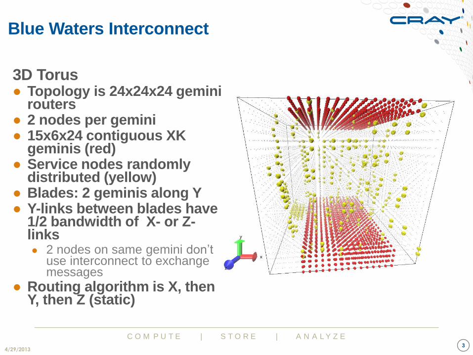
3D Torus ● Topology is 24x24x24 gemini

routers ● 2 nodes per gemini ● 15x6x24 contiguous XK

geminis (red) ● Service nodes randomly

distributed (yellow) ● Blades: 2 geminis along Y ● Y-links between blades have

1/2 bandwidth of X- or Z-links ● 2 nodes on same gemini don’t

use interconnect to exchange messages

● Routing algorithm is X, then Y, then Z (static)

3


Blue Waters Interconnect (cont’d)

10/7/2014 4

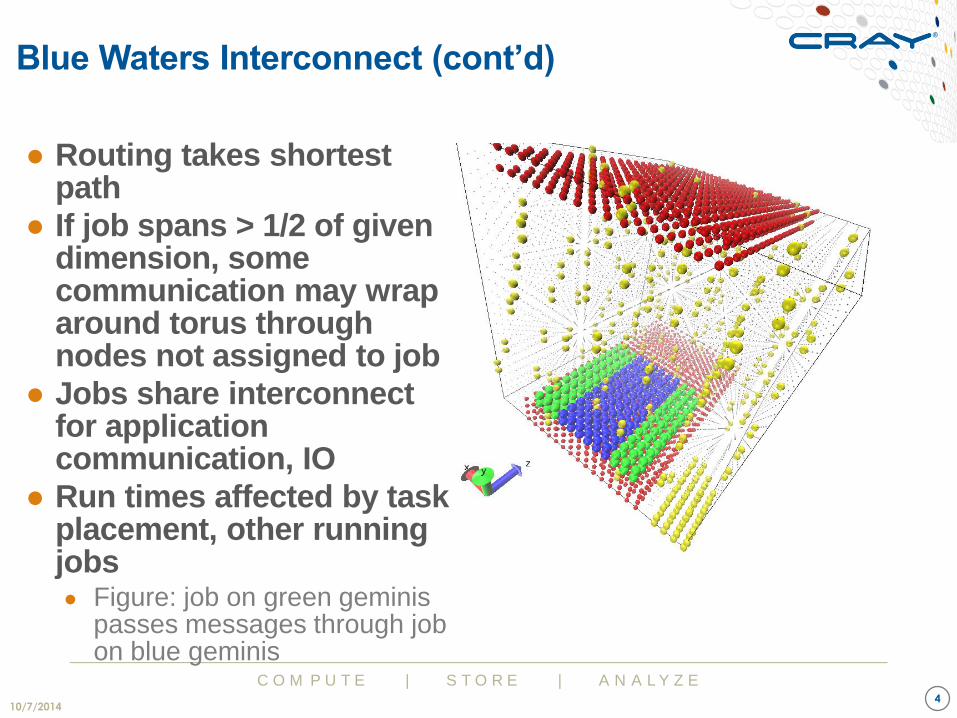
● Routing takes shortest path

● If job spans > 1/2 of given dimension, some communication may wrap around torus through nodes not assigned to job

● Jobs share interconnect for application communication, IO

● Run times affected by task placement, other running jobs ● Figure: job on green geminis

passes messages through job on blue geminis

Node Allocations: ALPS & Job Scheduler

10/9/2014 5

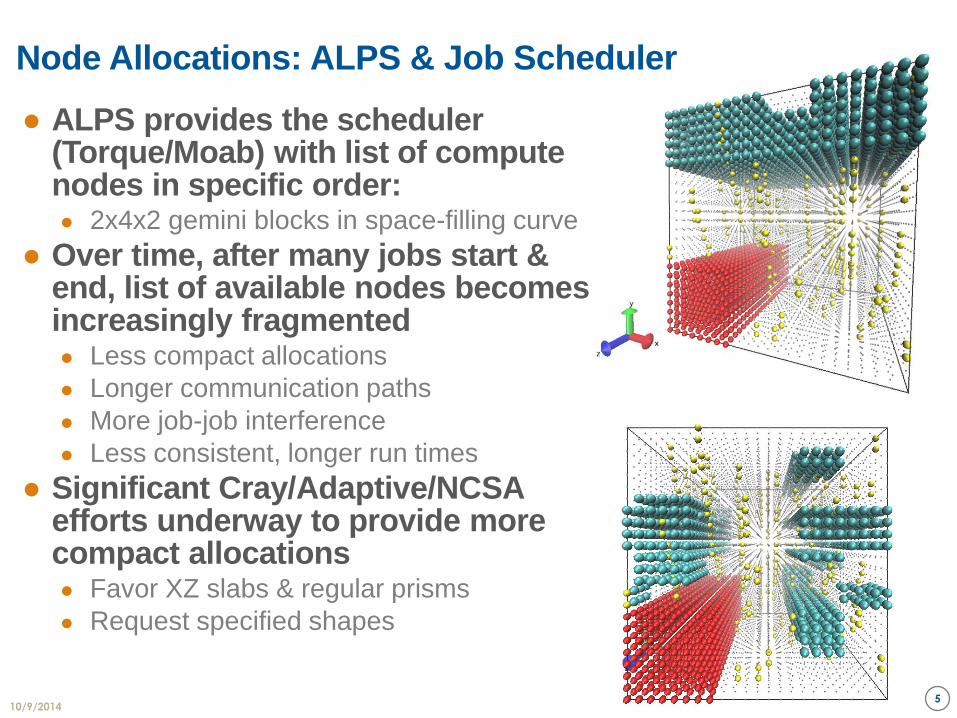
● ALPS provides the scheduler (Torque/Moab) with list of compute nodes in specific order: ● 2x4x2 gemini blocks in space-filling curve

● Over time, after many jobs start & end, list of available nodes becomes increasingly fragmented ● Less compact allocations

● Longer communication paths

● More job-job interference

● Less consistent, longer run times

● Significant Cray/Adaptive/NCSA efforts underway to provide more compact allocations ● Favor XZ slabs & regular prisms

● Request specified shapes


Task Placement and Interference

10/12/2014 6

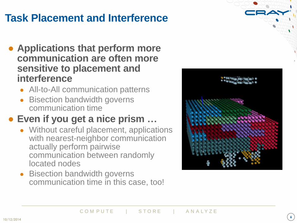
● Applications that perform more communication are often more sensitive to placement and interference ● All-to-All communication patterns

● Bisection bandwidth governs communication time

● Even if you get a nice prism … ● Without careful placement, applications

with nearest-neighbor communication actually perform pairwise communication between randomly located nodes

● Bisection bandwidth governs communication time in this case, too!


Topology-Aware Scheduling in Moab

10/7/2014 7

● NCSA/Cray/Adaptive collaboration

● Goals

● Improve application scaling on Cray XE/XK systems through better-

localized job placement

● Improve application run-time consistency by minimizing job-job interference due to application communication

● Increase system throughput by maintaining good utilization

● Approach

● Allocate nodes in contiguous prisms

● Eliminate interference: allocation either spans a torus dimension, or

spans half or less of a dimension (avoids torus wrap)

● Favor xz slabs to maximize bisection bandwidth

● Boost utilization by more freely placing jobs that are not affected by

application communication

● Allow applications to request specific allocation shapes


T-A Scheduler’s Criteria for Allocation Shape

10/12/2014 8

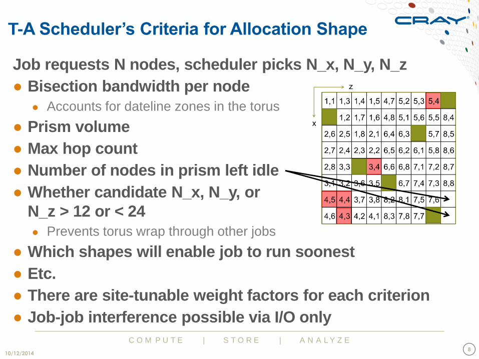
Job requests N nodes, scheduler picks N_x, N_y, N_z

● Bisection bandwidth per node

● Accounts for dateline zones in the torus

● Prism volume

● Max hop count

● Number of nodes in prism left idle

● Whether candidate N_x, N_y, or

N_z > 12 or < 24

● Prevents torus wrap through other jobs

● Which shapes will enable job to run soonest

● Etc.

● There are site-tunable weight factors for each criterion

● Job-job interference possible via I/O only


Weak Scaling for Application Using All-to-All

10/7/2014 9

3D FFTs: N^3 grid points, P tasks ● 1D FFT computation time

~ N^3 * (const. + log N) ● Transpose communication time

~ All-to-All time ● All-to-All time ~ Data volume/bandwidth

~ N^3/bandwidth

● For weak scaling experiments ● N^3/P is held constant ● Computation time grows slowly with P ● Communication time ~ P/bandwidth

● Thus, near-ideal weak scaling requires ● Bisection bandwidth ~ P ● i.e., constant per-node bisection bandwidth

● Minimizing time to solution means maximizing bisection bandwidth per node


Bisection Bandwidth: Full System

10/7/2014 10

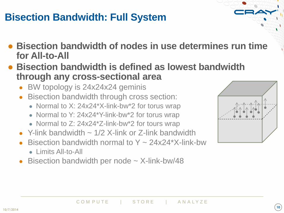
● Bisection bandwidth of nodes in use determines run time for All-to-All

● Bisection bandwidth is defined as lowest bandwidth through any cross-sectional area ● BW topology is 24x24x24 geminis

● Bisection bandwidth through cross section: ● Normal to X: 24x24*X-link-bw*2 for torus wrap

● Normal to Y: 24x24*Y-link-bw*2 for torus wrap

● Normal to Z: 24x24*Z-link-bw*2 for tours wrap

● Y-link bandwidth ~ 1/2 X-link or Z-link bandwidth

● Bisection bandwidth normal to Y ~ 24x24*X-link-bw ● Limits All-to-All

● Bisection bandwidth per node ~ X-link-bw/48

y


Bisection Bandwidth: Slab w/N Geminis in Y

10/12/2014 11

● Consider subset of nodes: 24xNx24

● Bisection bandwidth through cross section: ● Normal to X: N*24*X-link-bw*2 for torus wrap ~ 2*Nx24*X-link-bw

● Normal to Y: 24x24*Y-link-bw * f(N) ~ f(N)*12x24*X-link-bw

● Normal to Z: 24xN*Z-link-bw*2 for tours wrap ~ 2*Nx24*X-link-bw

● Bisection bandwidth per node for any N ● ~ X-link-bw/24 for N=1 through N=6 [since f(N) = 1 and 2N <= 12]

● ~ X-link-bw/(4*N) for N=6 through N=12 [since f(N) = 1 and 2N >= 12]

● ~ X-link-bw*(N-1)/(23*2*N) for N > 12 [since f(N) = 2*(N-1)/(24-1)]


Bisection Bandwidth: Small slab

10/7/2014 12

● Consider smaller node counts, e.g., 12x6x12 so no wrapping occurs ● ~1700 nodes

● Bisection bandwidth through cross section: ● Normal to X: 6*12*X-link-bw ~ 12*6*X-link-bw

● Normal to Y: 12*12*Y-link-bw ~ 12*6*X-link-bw

● Normal to Z: 12*6*Z-link-bw ~ 12*6 X-link-bw

● Bisection bandwidth per node ● ~ X-link-bw/24

● Same good value as for 24x6x24 geminis


T-A Scheduler Allows User-Specified Shapes

10/10/2014 13

Why would one want to specify allocation shape?

1. Application requires maximum bisection bandwidth ● Scheduler should not consider other cost factors

2. Application communicates more in some dimensions than others ● Same amount of communication per grid cell in each direction

● Per-node tiling with 2M by M by 2M grid cells anticipates 2X faster links along x and z

● Want cubic allocation, not xz slab

● Need to provide custom MPI rank order (Craypat or grid_order) to place groups of neighboring ranks on each node

3. Tasks are to be placed on the torus in near-optimal manner (Topaware)


Prism Geometry Requests

10/12/2014 14

How to get a particular prism shape instead of allowing the T-A scheduler to choose for you

● To get a particular prism shape #PBS -l nodes=576:ppn=32:xe

#PBS -l geometry=12x2x12

● Multiple geometry choices #PBS -l nodes=576:ppn=32:xe

#PBS -l geometry=12x2x12/12x4x6/6x4x12


Virtual Topologies and Task Placement

10/7/2014 15

● Many applications define Cartesian grid virtual topologies ● MPI_CartCreate

● Roll your own (i, j, …) virtual coordinates for each rank

● Craypat rank placement ● Automatic generation of rank order based on detected grid topology

● grid_order tool ● User specifies virtual topology to obtain rank order file

● Node list by default is in whatever order ALPS/MOAB provide

● These tools can be very helpful in reducing off-node communication, but they do not explicitly place neighboring groups of partitions in virtual topology onto neighboring nodes in torus


Examples: 2D Virtual topology

10/7/2014 16

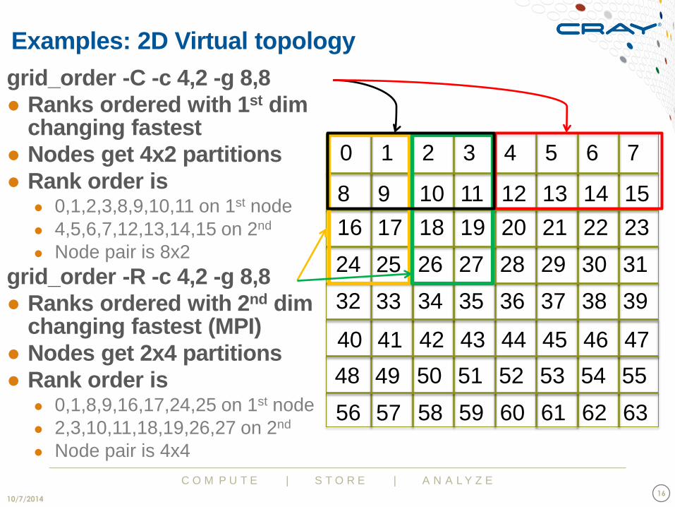
grid_order -C -c 4,2 -g 8,8

● Ranks ordered with 1st dim changing fastest

● Nodes get 4x2 partitions

● Rank order is ● 0,1,2,3,8,9,10,11 on 1st node

● 4,5,6,7,12,13,14,15 on 2nd

● Node pair is 8x2

grid_order -R -c 4,2 -g 8,8

● Ranks ordered with 2nd dim changing fastest (MPI)

● Nodes get 2x4 partitions

● Rank order is ● 0,1,8,9,16,17,24,25 on 1st node

● 2,3,10,11,18,19,26,27 on 2nd

● Node pair is 4x4

16 18 19 20 21 22 23 17

24 26 27 28 29 30 31 25

32 34 35 36 37 38 39 33

40 42 43 44 45 46 47 41

48 50 51 52 53 54 55 49

56 58 59 60 61 62 63 57

8 10 11 12 13 14 15 9

1 0 2 3 4 5 6 7

Examples: WRF (2D Virtual Topology)

10/7/2014 17

190x384 partitions ● Default layout ● 16x1 partitions per

node ● Every task needs

off-gemini communication

● 18% faster using grid_order -C -c 2,8 -g 190,384

● 2x8 partitions per node

● Interior stencils on same gemini

● 8x2 not nearly as good

Stencil

Node 0

Node 1

Node 0 Node 1


Examples: 3D Cubed Sphere

10/7/2014 18

SPECFEM3D_GLOBE

● Quad element unstructured grid

● 5419 nodes, 32 tasks per node

● Craypat detected a 1020x170 grid pattern (8 less than # tasks) ● On-node 81% of total B/task w/Custom

● On-node 48% of total B/task w/SMP

● Found best performance with

grid_order –R -c 4,1 -g 1020,170 ● Each node gets eight 4x1 patches

● Also tried –c 8,2, etc.

● 16% speedup over SMP ordering


Examples: 4D Virtual Topology

10/7/2014 19

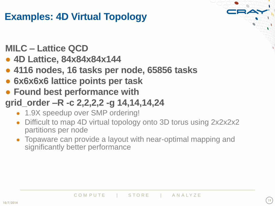
MILC – Lattice QCD

● 4D Lattice, 84x84x84x144

● 4116 nodes, 16 tasks per node, 65856 tasks

● 6x6x6x6 lattice points per task

● Found best performance with

grid_order –R -c 2,2,2,2 -g 14,14,14,24 ● 1.9X speedup over SMP ordering!

● Difficult to map 4D virtual topology onto 3D torus using 2x2x2x2 partitions per node

● Topaware can provide a layout with near-optimal mapping and significantly better performance


Topaware: Going Beyond Simple Rank Reordering

10/7/2014 20

Significant improvement possible

● Can we place tasks on a given set of nodes so that virtual neighbors are nearby on torus? ● Difficult problem for arbitrary node lists

● Possibly helpful library: Hoefler’s LibTopoMap http://htor.inf.ethz.ch/research/mpitopo/libtopomap/

● Not widely used – steep learning curve, etc.

● Can we specify size of prism of geminis and directly map virtual topology to torus? ● Presence of service & down nodes complicates this

● T-A scheduler can provide specified number of geminis in each z-pencil through an allocation ● This is exactly what Topaware needs to get good layouts

● With Topaware, NO NEED TO MODIFY APPLICATION!

http://htor.inf.ethz.ch/research/mpitopo/libtopomap/

http://htor.inf.ethz.ch/research/mpitopo/libtopomap/


Topaware Integrated with T-A Scheduler

10/7/2014 21

● Provides near optimal task

mapping for 2, 3, & 4D

Cartesian grid virtual topologies

● Prism is extended along z by max

number of service/down nodes in

any z-pencil

● Determines multiple valid layouts

and evaluates layout quality

● Allows unbalanced layouts

● Nodes on prism boundaries may have

fewer tasks

● Enables good layouts for more virtual

topology sizes

● Scheduler ensures allocation has

required gemini count in each

z-pencil


10/12/2014 22

8,1 8,2 8,3 8,4 8,5 8,6 8,7 8,8

2,2 2,3 2,4 2,5 2,6 2,7 2,8

1,1 1,2 1,3 1,4 1,5 1,6 1,7 1,8

3,1 3,2 3,3 3,4 3,5 3,6 3,7 3,8

4,1 4,2 4,3 4,4 4,5 4,6 4,7 4,8

5,1 5,2 5,3 5,4 5,5 5,6 5,7 5,8

6,1 6,2 6,3 6,4 6,5 6,6 6,7 6,8

7,1 7,2 7,3 7,4 7,5 7,6 7,7 7,8

z

x 2,1

Ideal 8x8 layout on ideal system, 1 rank per router (!)

LAYOUT EXAMPLE: 2D Virtual Topology


10/12/2014 23

4,6 4,3 4,2 4,1 8,3 7,8 7,7 8,8

1,2 1,7 1,6 4,8 5,1 5,6 5,5 8,4

1,1 1,3 1,4 1,5 4,7 5,2 5,3 5,4

2,6 2,5 1,8 2,1 6,4 6,3 3,7 5,7 8,5

2,7 2,4 2,3 2,2 6,5 6,2 6,1 5,8 8,6

2,8 3,3 5,3 3,4 6,6 6,8 7,1 7,2 8,7

3,1 3,2 3,6 3,5 6,5 6,7 7,4 7,3 8,8

4,5 4,4 3,7 3,8 8,2 8,1 7,5 7,6

z

x 2,1

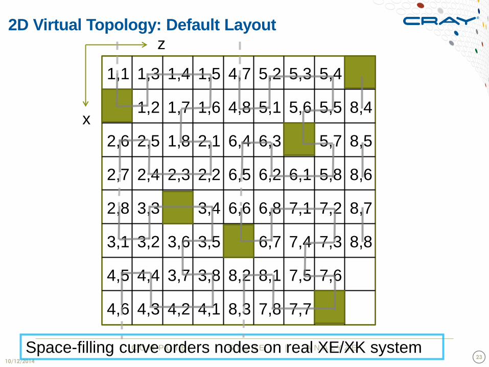
Space-filling curve orders nodes on real XE/XK system

2D Virtual Topology: Default Layout


10/12/2014 24

4,6 4,3 4,2 4,1 8,3 7,8 7,7 8,8

1,2 1,7 1,6 4,8 5,1 5,6 5,5 8,4

1,1 1,3 1,4 1,5 4,7 5,2 5,3 5,4

2,6 2,5 1,8 2,1 6,4 6,3 3,7 5,7 8,5

2,7 2,4 2,3 2,2 6,5 6,2 6,1 5,8 8,6

2,8 3,3 5,3 3,4 6,6 6,8 7,1 7,2 8,7

3,1 3,2 3,6 3,5 6,5 6,7 7,4 7,3 8,8

4,5 4,4 3,7 3,8 8,2 8,1 7,5 7,6

z

x 2,1

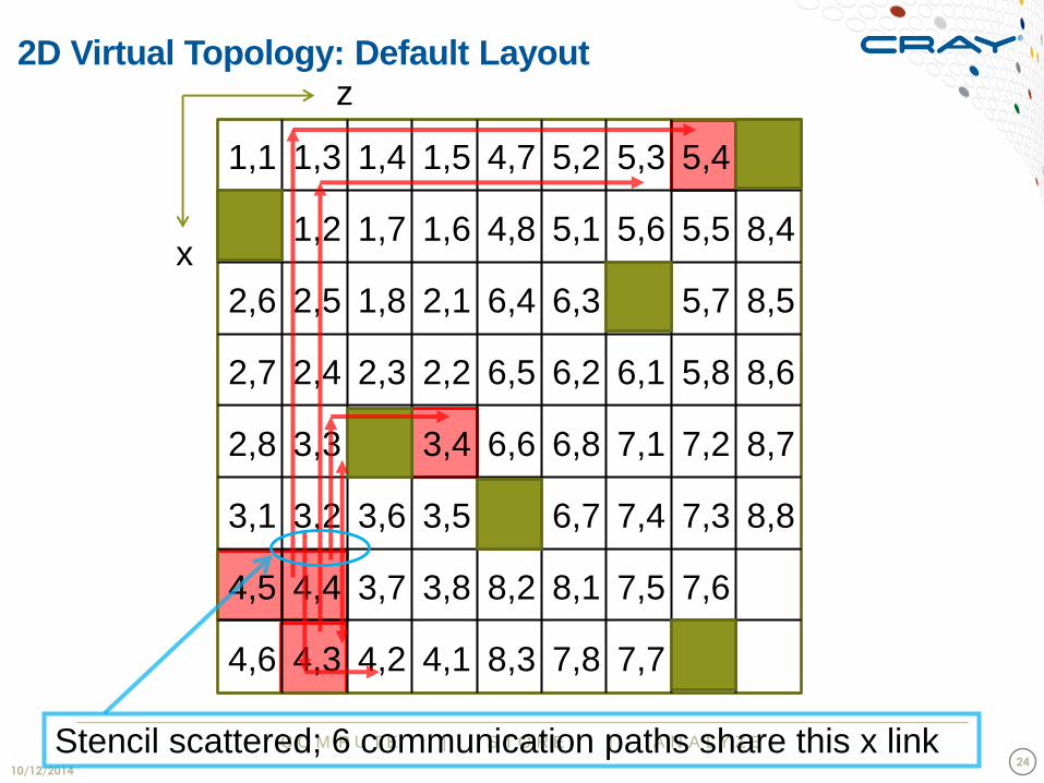
Stencil scattered; 6 communication paths share this x link

2D Virtual Topology: Default Layout


10/12/2014 25

8,1 8,2 8,3 8,4 8,5 8,6 8,7 8,8 8,8

2,1 2,2 2,3 2,4 2,5 2,6 2,7 2,8

1,1 1,2 1,3 1,4 1,5 1,6 1,7 1,8

3,1 3,2 3,3 3,4 3,5 3,6 3,7 3,7 3,8

4,1 4,2 4,3 4,4 4,5 4,6 4,7 4,8

5,1 5,2 5,3 5,3 5,4 5,5 5,6 5,7 5,8

6,1 6,2 6,3 6,4 6,5 6,5 6,6 6,7 6,8

7,1 7,2 7,3 7,4 7,5 7,6 7,7 7,8

z

x 2,1

Topaware keeps ranks in desired z-pencils

2D Virtual Topology: Topaware Layout


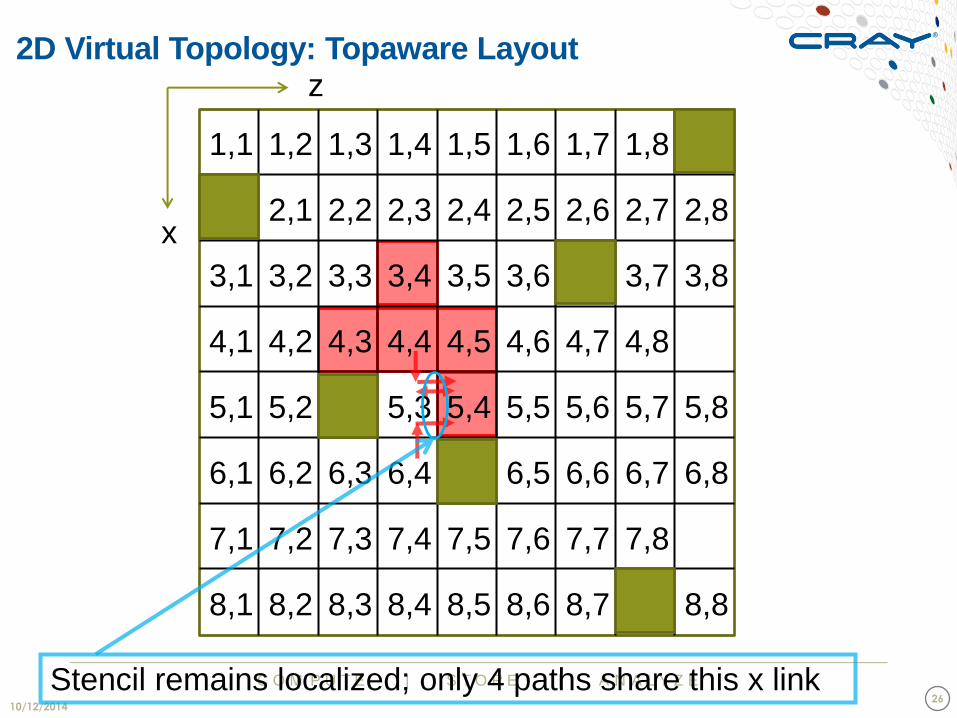
10/12/2014 26

8,1 8,2 8,3 8,4 8,5 8,6 8,7 8,8 8,8

2,1 2,2 2,3 2,4 2,5 2,6 2,7 2,8

1,1 1,2 1,3 1,4 1,5 1,6 1,7 1,8

3,1 3,2 3,3 3,4 3,5 3,6 3,7 3,7 3,8

4,1 4,2 4,3 4,4 4,5 4,6 4,7 4,8

5,1 5,2 5,3 5,3 5,4 5,5 5,6 5,7 5,8

6,1 6,2 6,3 6,4 6,5 6,5 6,6 6,7 6,8

7,1 7,2 7,3 7,4 7,5 7,6 7,7 7,8

z

x 2,1

Stencil remains localized; only 4 paths share this x link

2D Virtual Topology: Topaware Layout


Topware 2.0: Practical Near-Optimal Layouts

10/7/2014 27

● Helps you choose prism geometries/node counts that will accommodate your decomposed problem

● At run time, provides near-optimal layout matching the allocated prism

● Steps 1. Run Topaware on login node to find desirable geometries

2. Submit batch job requesting those geometries

3. Invoke Topaware again within batch job to place tasks on nodes in that allocation

4. Use aprun to launch job using node order and custom rank order generated by Topaware


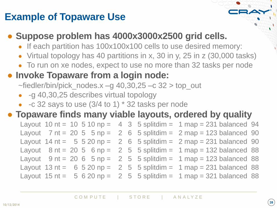
Example of Topaware Use

10/12/2014 28

● Suppose problem has 4000x3000x2500 grid cells. ● If each partition has 100x100x100 cells to use desired memory:

● Virtual topology has 40 partitions in x, 30 in y, 25 in z (30,000 tasks)

● To run on xe nodes, expect to use no more than 32 tasks per node

● Invoke Topaware from a login node: ~fiedler/bin/pick_nodes.x –g 40,30,25 –c 32 > top_out

● -g 40,30,25 describes virtual topology

● -c 32 says to use (3/4 to 1) * 32 tasks per node

● Topaware finds many viable layouts, ordered by quality Layout 10 nt = 10 5 10 np = 4 3 5 splitdim = 1 map = 231 balanced 94

Layout 7 nt = 20 5 5 np = 2 6 5 splitdim = 2 map = 123 balanced 90







Using Topaware to Find Good Layouts

10/12/2014 29

● Topaware layouts for 40x30x25 topology Layout 10 nt = 10 5 10 np = 4 3 5 splitdim = 1 map = 231 balanced 94 Layout 7 nt = 20 5 5 np = 2 6 5 splitdim = 2 map = 123 balanced 90 Layout 14 nt = 5 5 20 np = 2 6 5 splitdim = 2 map = 231 balanced 90 Layout 8 nt = 20 5 6 np = 2 5 5 splitdim = 1 map = 132 balanced 88 Layout 9 nt = 20 6 5 np = 2 5 5 splitdim = 1 map = 123 balanced 88 Layout 13 nt = 6 5 20 np = 2 5 5 splitdim = 1 map = 231 balanced 88 Layout 15 nt = 5 6 20 np = 2 5 5 splitdim = 1 map = 321 balanced 88 Valid BALANCED layout 10 has map = 231 ppn = 30 numnodes = 1000 dims(p2v(1)) nt(1) np(p2v(1)) = 30 10 3 Dim 2 on 10 geminis in torus x dims(p2v(2)) nt(2) np(p2v(2)) = 25 5 5 Dim 3 on 5 geminis in torus y dims(p2v(3)) nt(3) np(p2v(3)) = 40 10 4 Dim 1 on 10 geminis in torus z percent_used is 100 Uses 100% of nodes in prism bal_metric is 100 All nodes get same number of active tasks (“balanced”) ppn_metric is 93 Uses 30/32 integer cores per node p2c_metric is 80 per node pair “volume to surface ratio” compared to cube qual_metric is 94 Geometric mean of above factors


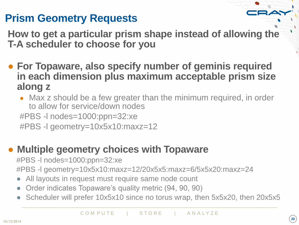
Prism Geometry Requests

10/12/2014 30

How to get a particular prism shape instead of allowing the T-A scheduler to choose for you

● For Topaware, also specify number of geminis required in each dimension plus maximum acceptable prism size along z ● Max z should be a few greater than the minimum required, in order

to allow for service/down nodes

#PBS -l nodes=1000:ppn=32:xe

#PBS -l geometry=10x5x10:maxz=12

● Multiple geometry choices with Topaware #PBS -l nodes=1000:ppn=32:xe

#PBS -l geometry=10x5x10:maxz=12/20x5x5:maxz=6/5x5x20:maxz=24

● All layouts in request must require same node count

● Order indicates Topaware’s quality metric (94, 90, 90)

● Scheduler will prefer 10x5x10 since no torus wrap, then 5x5x20, then 20x5x5


Running Batch Jobs Using Topaware

10/12/2014 31

● Suppose we requested 10x5x10 geminis (only) # Get the node list to confine Topaware’s scans cat $PBS_NODEFILE | uniq | tr '\n' ',' | sed -e 's/,$/\n/' > node_list # Invoke topaware in batch mode using this node list ~fiedler/bin/pick_nodes.x -M 2 -U node_list -g 40,30,25 -c 32 >& top_out # Scan top_out for the first successful layout, where it says: # SUCCESS Layout 10 nt = 10 5 10 np = 4 3 5 splitdim = 1 map = 231 balanced 94 # The node list has been written to a file called nodes-10-1000_10_5_10_4_3_5 # The rank list has been written to a file called # MPICH_RANK_ORDER-10-1000_10_5_10_4_3_5_1 … # Set up to use custom rank order cp MPICH_RANK_ORDER-1000_10_5_10_4_3_5_1 MPICH_RANK_ORDER export MPICH_RANK_REORDER_METHOD=3 # Run application using Topaware’s node list, plus task affinity and core specialization aprun -l nodes-10-1000_10_5_10_4_3_5 -n 30000 -N 30 -cc 0,1,2,3,4,5,6,7,8,9,10,11,12,13,14,16,17,18,19,20,21,22,23,24,25,26,27,28,29,30 -r 1 ./my_app.exe


Examples: 4D Halo Exchanges

10/12/2014 32

Compare default ordering, grid_order, and Topaware on same set of nodes (selected by Topaware).

● 4D Lattice, 144x144x144x288 points

● 12x16x16x16 partitions

● 1536 nodes, 32 tasks per node, 49152 tasks


● Topaware: each node gets 1x2x2x8 tasks

● Prism: 24x2x24 geminis

● Run times ● Default placement (SMP): 0.0240 s

● grid_order -C -g 12,16,16,16 -c 2,2,2,4: 0.0245 s (worse than default!)

● Topaware: 0.0127 s (1.9X < default!!)


Application Results on Blue Waters

4/29/2013 33

MILC – Lattice QCD

● 4D Lattice, 84x84x84x144

● 4116 nodes, 16 tasks per node


● Entire 4th dimension on each node pair ● Remaining 3 dimensions mapped like any 3D virtual topology

● 14x7x21 geminis (in 14x7x23 prism from T-A scheduler)

● 1x2x1x16 partitions per node pair

● 3.7X faster than default SMP placement ● 2.1X faster than when using grid_order –c 2,2,2,2 on same geminis!


Results on Blue Waters for Cybershake

4/10/2013 34

● Seismic waves ● 3D virtual topology ● http://hypocenter.usc.edu/research/BlueW

aters/XtremeS_CyberShake_final.pdf


Topaware Unbalanced Layouts

10/12/2014 35

● Virtual topology: 32 by 32 by 32, up to 32 tasks per node


Layout 2 nt = 11 8 8 np = 3 4 4 splitdim = 2 map = 123 unbalanced 81




● For 11x8x8, node pairs in first 10 yz planes get 3*4*4 = 48

active tasks (total of 30720/32768 tasks)

● Node pairs in 11th yz plane get 2*4*4 = 32 active tasks

(total of 2048/32768 tasks)

● If load were balanced, each node would do

32768 tasks / (11*8*8*2 nodes) = 23.3 units of work

● Unbalanced layout puts 24 units of work (only 3% more!)

on most nodes


Topaware Unbalanced Layouts: Results

10/12/2014 36

● Halo exchanges for virtual topology: 32 by 32 by 32

● For < 32 tasks per node, core specialization enables overlap of

communication and copying data to/from message buffers

Placement Communication

time (ms)

Tasks per node Per node

speedup

Default 8x8x8 11.315 32 1

Grid_order

8x8x8

7.722 32 1.5

Topaware 8x8x8 2.771 32 4.1

Topaware 11x8x8

(unbalanced)

1.147 24 7.4

Topaware 8x8x11

(unbalanced)

1.214 24 7.0

Topaware 11x8x7

(unbalanced)

1.580 30 6.7

Topaware 7x8x11

(unbalanced)

1.690 30 6.3


Topaware Unbalanced Layouts: What’s Needed

10/12/2014 37

● aprun will create same number of tasks on every node

● N total tasks in MPI_COMM_WORLD communicator

● Application needs modification

● Determine M, the number of partitions in desired virtual topology

● M < N

● Use MPI_COMM_SPLIT to create new communicator with M ranks

● Solve the problem using only ranks in the smaller communicator

● Topaware puts the idle ranks on the node pairs along the

appropriate surface(s) of the prism


Concluding Remarks

10/12/2014 38

● We hope to deploy the new Topology-Aware scheduler in

the Blue Waters production environment soon

● Excellent results obtained so far in scale tests

● Expect most applications to benefit without user effort

● Allocates jobs in prisms of gemini routers

● Better, more consistent run times

● Improved scaling

● Limited impact on queue wait times

● Applications with grid topologies can leverage Topaware

● Provides near-optimal task layouts for most decompositions

● Automatically selects appropriate prism sizes & node counts

● May improve communication/computation overlap

● Unbalanced layouts may be surprisingly efficient

improving performance and scaling on blue waters … · communication time in this case, too! ......

Documents