improving settleability and enhancing biological ......improving settleability and enhancing...
TRANSCRIPT
Improving Settleability and Enhancing Biological Phosphorus Removal through the
Implementation of Hydrocyclones
Claire M. Welling
Thesis submitted to the faculty of the Virginia Polytechnic Institute and State University
in partial fulfillment of the requirements for the degree of
Master of Science
In
Environmental Engineering
Charles B. Bott, Chair
Gregory D. Boardman, Co-chair
John T. Novak
November 17th
2015
Blacksburg, VA
Keywords: settleability, biological phosphorus removal, external selector, hydrocyclone
Copyright 2015, Claire M. Welling
Improving Settleability and Enhancing Biological Phosphorus Removal through the
Implementation of Hydrocyclones
Claire M. Welling
ABSTRACT
For many wastewater treatment plants, mixed liquor settling is a limiting factor for treatment
capacity. However, by creating a balance of granules and flocs, higher settling rates may be
achieved. Granules can be defined at discrete particles that do not need bio-flocculation to settle.
Through the use of a hydraulic external selector, it is possible to select for dense granules within
an existing process which leads to increased settleability. The dense granules are recycled and
have the characteristics to achieve not only high settling rates, but also provide a means for
biological nutrient removal (Morgenroth and Sherden, 1997). Biological phosphorus removal
occurs within the granules without the need for a formal anaerobic selector. Phosphorus
accumulating organisms (PAO) and denitrifying PAO (DPAO) are dense and become contained
within the granules. PAO and DPAO also have the advantageous characteristic of being more
dense than glycogen accumulating organisms (GAO), resulting in selective pressure against GAO
(Morgenroth and Sherden, 1997). The granules form stratified layers; ordinary aerobic
heterotrophic growth and nitrification occurring in the aerobic outer layer, denitrification in the
anoxic layer below, and phosphate removal occurring periodically in the anaerobic core, allowing
for not only phosphorus removal, but also nitrogen consumption.
This technology utilizes hydrocyclones for the purpose of improving sludge settling and has been
successfully implemented at the Strass wastewater treatment plant in Austria. Hydrocyclones
receive mixed liquor tangentially and separate light solids from more dense solids through their
tapered shape, increasing the velocity of liquid as it moves downward and allowing for selection
of a certain solids fraction. The hydrocyclones select for dense granules through the underflow
which are recycled back to the process. The lighter solids are sent to the overflow which
represents the waste activated sludge (WAS). Filaments often occur in lighter solids and can
exacerbate settleability issues. By wasting lighter solids, filaments will be wasted as well
resulting in increased settleability. The Hampton Roads Sanitation District’s (HRSD) James River
Wastewater Treatment Plant (JR) located in Newport News, VA utilizes an IFAS system. JR
achieves some unreliable biological phosphorus removal in warmer temperatures as PAO exist in
the bulk liquid but cannot proliferate without a formal anaerobic zone. Chemical phosphorus
iii
removal using ferric chloride addition is used to achieve low effluent phosphorus concentrations.
The plant routinely experiences moderate settleability issues with a 4.5 year average SVI of 141
mL/g and a 90th percentile SVI of 179 mL/g. JR is rated at 20 MGD and utilizes a 4-stage
Bardenpho configured in an IFAS system. This project includes a full scale implementation of
hydrocyclones for improving settleability and stabilizing biological phosphorus removal
(reduction in ferric chloride demand) without installation of a formal anaerobic zone.
Plant data collected for James River indicate a reduction in ferric chloride usage as biological
phosphorus removal remained constant during the last 2 months of data collection. A reduction in
Ferric addition was noticed approximately 3 months after the cyclones were under full operation.
2015 SVI data shows a slight decrease in the average SVI5 decreasing from 292 mL/g to 248
mL/g after cyclones were installed, while the SVI30 value remained fairly constant at an average
of 138±70 mL/g. The floc density of the aeration effluent mixed liquor increased steadily over
time from 1.050 to 1.071 g/mL. The average density of the cyclone overflow and underflow was
1.078±.005 g/mL and 1.033±.002 g/mL respectively, indicating that the denser sludge was being
selectively retained while wasting the lighter sludge. Classification of settling rate data indicated
that granule percentage increased from 0% during the pre-cyclone period to up to 24-40% during
the cyclone operation period. Biological phosphorus activity was present in the ML at similar
rates when comparing pre-cyclone and post-cyclone periods, indicating that the hydrocyclones
may not have had a large effect on the biological phosphorus activity. AOB and NOB activity
measurements in the cyclone overflow, underflow, and feed confirm that nitrifiers were not being
selectively wasted from the system. Filament data taken from the plant and microscopic analysis
showed that some filaments were present in the system but not at levels that would hinder
settleability or cause foaming. It was also shown through staining and microscopy that PAO were
present while the GAO population was minimal throughout the study.
iv
Acknowledgements
First and foremost I would like to thank my amazing advisor Dr. Charles Bott for all of
his guidance and knowledge. His contagious enthusiasm effects all around him. I cannot
express my gratitude enough for being given this opportunity to receive a higher
education and conduct innovative research. I would also like to thank Dr. Gregory
Boardman and Dr. John Novak for serving on my committee and for their valuable input.
Thank you to Hampton Roads Sanitation District for the funding and support.
I would like to recognize Dr. Mark Miller and Dr. Pusker Regmi for introducing me to
the pilot plant at HRSD, which included answering endless questions and training me on
all lab procedures. Their breadth of knowledge was a valuable resource and I greatly
appreciate the opportunity to work with such gifted people. Ryder Bunce and Dana
Fredericks also played an important role in my initial training and were great friends
throughout the process. Once arriving at Virginia Tech, my fellow HRSD interns Mike
Sadowski and Peerawat Noon Charuwat were in the majority of my classes. Without their
optimistic attitudes and our frequent study sessions I would have barely gotten by. They
are both incredibly intelligent and on top of that never failed to make me smile.
Upon my return to the Hampton Roads area, Stephanie Klaus introduced me to the James
River WWTP. Not only did she thoroughly explain the processes at the plant and answer
any questions I had, but her support and friendship became crucial to my growth as a
student, intern, and person. Her curiosity and drive are inspiring and she will always be a
role model to me. I would also like to thank Arba Williamson, Amanda Kennedy, Jon
DeArmond, Johnnie Godwin, and Matthew Elliot for always helping when I needed it
and being great friends.
Lastly, I would like to thank my family, especially my siblings; Katherine, Sam, Grace,
Charlie, Max, Rachel, and Tess, for being my main supporters and molding me into the
person I am today.
v
Table of Contents 1. Introduction and Project Objectives .................................................................................... 1
1.1 Project Background ................................................................................................ 1
1.2 Hydrocyclone Installation ...................................................................................... 2
1.3 Project Objectives .................................................................................................. 3
2. Literature Review ................................................................................................................ 5
2.1 Settleability ............................................................................................................. 5
2.1.1 Overview ....................................................................................................... 5
2.1.1.1 Density of Sludge ................................................................................. 5
2.1.1.2 Clarifier Design .................................................................................... 6
2.1.2 Types of Settleability Issues .......................................................................... 6
2.1.2.1 Filamentous Bulking ............................................................................ 6
2.1.2.2 Pinpoint Floc ........................................................................................ 7
2.1.2.3 Viscous Bulking ................................................................................... 7
2.1.2.4 Dispersed Growth ................................................................................ 7
2.1.2.5 Blanket Rising...................................................................................... 7
2.1.2.6 Foam or Scum Formation .................................................................... 8
2.1.3 Filaments ....................................................................................................... 8
2.1.3.1 Filament Proliferation ........................................................................ 10
2.1.3.2 DO ...................................................................................................... 11
2.1.3.3 Filament Counting Methods and Characterization ............................ 11
2.1.4 Bulking Control ........................................................................................... 11
2.1.4.1 Kinetic and Metabolic Selection ........................................................ 12
2.1.4.2 Chemical Addition ............................................................................. 13
2.1.5 Selectors ...................................................................................................... 13
2.1.5.1 Aerobic............................................................................................... 14
2.1.5.2 Anoxic ................................................................................................ 14
2.1.5.3 Anaerobic ........................................................................................... 15
2.1.6 Classifying Selectors ................................................................................... 15
2.2 Biological Phosphorus Removal ........................................................................... 16
2.2.1 Background ................................................................................................. 16
2.2.2 PAO, DPAO, and GAO metabolism ........................................................... 18
2.2.2.1 PAO ................................................................................................... 18
2.2.2.2 GAO ................................................................................................... 20
2.2.2.3 PAO/GAO competition ...................................................................... 21
2.2.2.4 DPAO ................................................................................................ 23
2.2.3 Conditions Favoring EBPR ......................................................................... 23
2.2.3.1 Low Organic Loading ........................................................................ 25
2.2.3.2 DO ...................................................................................................... 25
2.2.4 Processes ..................................................................................................... 26
2.3 Granular Sludge .................................................................................................... 26
2.3.1 Background ................................................................................................. 26
2.3.2 Settleability .................................................................................................. 27
2.3.3 Formation .................................................................................................... 28
2.3.4 Biological Nutrient Removal ....................................................................... 29
2.3.5 Microbiology ............................................................................................... 30
2.4 Hydrocyclones ...................................................................................................... 31
2.5 Measurements for Settleability Characterization .................................................. 32
2.5.1 Sludge Volume Index .................................................................................. 33
2.5.2 Zone Settling Velocity................................................................................. 34
vi
2.5.3 Solids Flux ................................................................................................... 34
2.5.3.1 Vesilind .............................................................................................. 36
2.5.4 Classification of Settling Rates Tests .......................................................... 39
2.5.4.1 Limit of Stokian Settling .................................................................... 39
2.5.4.2 Surface Overflow Rate ....................................................................... 40
2.5.4.3 Threshold of Flocculation .................................................................. 40
3. Methods and Materials ...................................................................................................... 42
3.1 Plant Setup ............................................................................................................ 42
3.2 Cyclone Data ......................................................................................................... 44
3.3 Plant Data .............................................................................................................. 45
3.4 Sludge Volume Index (SVI) ................................................................................ 45
3.5 Zone Settling Velocity .......................................................................................... 46
3.6 Solids Flux ............................................................................................................ 46
3.7 Classification of Settling Rates ............................................................................. 47
3.7.1 Limit of Stokian Settling (LOSS) ............................................................... 47
3.7.2 Threshold of Flocculation (TOF) ............................................................... 47
3.7.3 Surface Overflow Rate (SOR) .................................................................... 48
3.8 Floc Density .......................................................................................................... 49
3.9 Filament Quantification and Identification ........................................................... 50
3.10 PAO Activity Tests ............................................................................................. 50
3.11 AOB and NOB Activity Tests ............................................................................ 51
3.12 Tank Profiling ..................................................................................................... 52
4. Results and Discussion ...................................................................................................... 53
4.1 Cyclone Data ......................................................................................................... 53
4.2 SVI ........................................................................................................................ 53
4.3 Solids Flux ............................................................................................................ 54
4.4 Settleability ........................................................................................................... 57
4.5 Classification of Settling Rates ............................................................................. 58
4.6 Floc Density .......................................................................................................... 59
4.7 Filaments ............................................................................................................... 61
4.7.1 Microscopic Analysis .................................................................................. 61
4.7.2 Plant Data .................................................................................................... 62
4.8 PAO Activity Tests ............................................................................................... 62
4.9 Phosphorus and Ferric Plant Data ......................................................................... 67
4.10 AOB and NOB Activity Tests ............................................................................ 68
4.11 Tank Profiling ..................................................................................................... 69
5. Conclusions and Engineering Significance ...................................................................... 71
References ......................................................................................................................... 73
Appendices ........................................................................................................................ 75
A. Phosphorus Activity .................................................................................................... 76
B. Phosphorus Uptake and Release Rates in Cyclone Sampling Points .......................... 78
C. AOB and NOB Activity in Cyclone Sampling Points ................................................ 79
D. Microscopic Analysis ................................................................................................. 80
E. Floc Density of Aeration Effluent and Cyclone Sampling Points .............................. 86
F. Floc Density SIP Calculation ...................................................................................... 87
G. Cyclone Data ............................................................................................................... 89
H. Plant Data .................................................................................................................... 92
I. Settleability ................................................................................................................. 99
J. Solids Flux Data ........................................................................................................ 100
K. Classification of Settling Rates ................................................................................. 103

vii
L. James River IFAS Tank Profiles............................................................................... 104
M. Supplemental Information ........................................................................................ 109
viii
List of Tables
Table 2.1 Filamentous Organism Characterization and Control ...................................................... 8
Table 2.2 Filamentous bacteria found in activated sludge and associated process conditions ....... 10
Table 2.3 Selector design guidelines recommended for aerobic, anoxic and anaerobic selectors.14
Table 2.4 Results of Phosphorus Uptake and Release Tests from 2005 WERF EBPR Study ....... 17
Table 2.5 Comparison of PAO/GAO Observations and Uptake and Release Test Results ........... 21
Table 2.6 Proposed metabolic features of the most known PAOs and GAOs ............................... 22
Table 4.1 Flow and Mass Split of Cyclone Underflow and Overflow for different nozzle sizes ... 53
ix
List of Figures
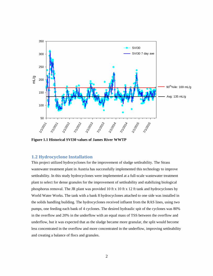
Figure 1.1 Historical SVI30 values of James River WWTP ............................................................ 2
Figure 2.1 PAO Metabolism Under Anaerobic and Aerobic/Anoxic Conditions .......................... 20
Figure 2.2 A Schematic of an Aerobic Granule with Stratified Layers .......................................... 30
Figure 2.3 Strass WWTP SVI over 3 year period, hydrocyclones installed beginning of year 2 .. 32
Figure 2.4 Relationship Between Solids Characteristics and Sedimentation Processes ................. 33
Figure 2.5 State Point Analysis of Solids Flux Curve .................................................................... 36
Figure 2.6 Settling function of Takács et al. (1991) incorporating the settling characteristics of
both dispersed and flocculated suspended solids ........................................................................... 39
Figure 2.7 (A) Determination of CSV working area as a region whereby no bio-flocculation
occurs (No significant decrease in TSS in the supernatant) Percentage TSS in effluent versus
ranging TSS of mixed liquor concentrations at an SOR of 1.5 m3/m2/h, and the grey area exhibits
discrete region. Discrete settling is defined as the initial region that is independent of the MLSS,
(B) Conceptual SOR curve with indication of the different solids fractions .................................. 41
Figure 3.1 James River IFAS Process Flow Diagram .................................................................... 43
Figure 3.2 Hydrocyclone Process and Instrumentation Diagram .................................................. .44
Figure 3.3 James River IFAS Tank Design .................................................................................... 52
Figure 4.1 2015 SVI5 and SVI30 of JR ........................................................................................ .54
Figure 4.2 Pre and Post-Cyclone Settling Velocity determined by SFA and the best fit Vesilind
Curve .............................................................................................................................................. 55
Figure 4.3 SFg curves pre and post cyclone installation. Calculated SFg curves using the Vesilind
settling velocity are shown as curves, actual data shown as points ................................................ 56
Figure 4.4 ISV of Cyclone Points adjusted to 2500 mg/L .............................................................. 57
Figure 4.5 Classification of Settling Rates of JR ML, SVI, and MLSS ......................................... 59
Figure 4.6 An example of the floc density analysis using Isopycnic centrifugation from 6/22/15 60
Figure 4.7 James River ML floc density of Aeration effluent and Cyclone Sampling Points ....... 61
Figure 4.8 Phosphorus Release and Uptake of Aeration Effluent .................................................. 64
Figure 4.9 Phosphorus Uptake and Release Rate of Cyclone Sample Points and Aeration Effluent
........................................................................................................................................................ 66
Figure 4.10 Ratio of Ferric Addition to Raw Influent Phosphorus and Phosphorus Removed ...... 67
Figure 4.11 Influent and Effluent Phosphorus concentrations ....................................................... 68
Figure 4.12 AOB and NOB activity in cyclone sampling points ................................................... 69
Figure 4.13 NO2, NOx, and NH4 of aeration effluent of JR ML................................................... 70

1
1. Introduction and Project Objectives
1.1 Project Background James River Wastewater Treatment Plant (JR) located in Newport News, Virginia is one of the 9
major wastewater treatment plants operating under the Hampton Roads Sanitation District
(HRSD). The plant was initially placed on-line in 1968. After undergoing expansion in the 1970’s
the plant has an average daily treatment capacity of 20 MGD. After receiving new nitrogen limits
of 12 mg/L, JR implemented a study in which an integrated fixed-film activated sludge (IFAS)
basin was installed in late 2007 in order to meet these requirements. After optimizing the IFAS
system design and achieving effluent TN of 8-12 mg/L, it became fully implemented in June
2009 (Rutherford, 2010). JR utilizes a 4-stage Bardenpho system.
James River currently has some settleability problems with an average SVI of 135 mL/g and a
90th percentile of 169 mL/g. Recent SVI data is seen if Figure 1.1. Poor settleability at JR is
exacerbated by relatively shallow, peripheral feed secondary clarifiers. It is unclear why JR has
such poor settleability as filament levels are low. James River also experiences some unreliable
biological phosphorus removal, with ferric addition added before the primary clarifiers and
secondary clarifiers to achieve a low total phosphorus (TP) effluent. JR’s TP effluent permit is 2
mg/L, but the plant aims to stay under 1 mg/L to make sure the total TP pounds limit for the
James River basin is met. Conventionally, enhanced biological phosphorus removal is achieved
through a separate anaerobic selector at the beginning of the biological reactors. This process uses
a large amount of carbon without much being used by phosphorus accumulating organisms
(PAO). The implementation of the hydrocyclones more efficiently utilizes carbon for PAO and
denitrifying PAO (DPAO).
2
1/1/
2011
7/1/
2011
1/1/
2012
7/1/
2012
1/1/
2013
7/1/
2013
1/1/
2014
7/1/
2014
1/1/
2015
7/1/
2015
mL/g
50
100
150
200
250
300
350
SVI30
SVI30 7 day ave
Avg: 135 mL/g
90th%ile: 169 mL/g
Figure 1.1 Historical SVI30 values of James River WWTP
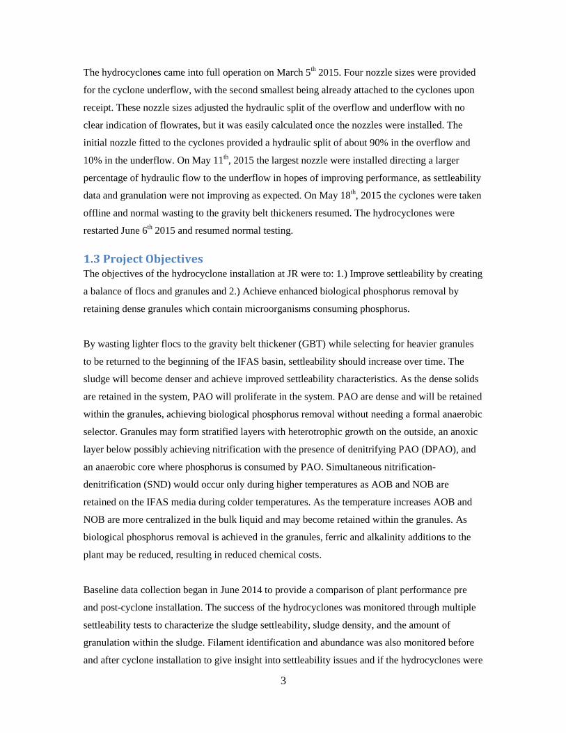
1.2 Hydrocyclone Installation This project utilized hydrocyclones for the improvement of sludge settleability. The Strass
wastewater treatment plant in Austria has successfully implemented this technology to improve
settleability. In this study hydrocyclones were implemented at a full-scale wastewater treatment
plant to select for dense granules for the improvement of settleability and stabilizing biological
phosphorus removal. The JR plant was provided 10 ft x 10 ft x 12 ft tank and hydrocyclones by
World Water Works. The tank with a bank 8 hydrocyclones attached to one side was installed in
the solids handling building. The hydrocyclones received influent from the RAS lines, using two
pumps, one feeding each bank of 4 cyclones. The desired hydraulic spit of the cyclones was 80%
in the overflow and 20% in the underflow with an equal mass of TSS between the overflow and
underflow, but it was expected that as the sludge became more granular, the split would become
less concentrated in the overflow and more concentrated in the underflow, improving settleability
and creating a balance of flocs and granules.
3
The hydrocyclones came into full operation on March 5th 2015. Four nozzle sizes were provided
for the cyclone underflow, with the second smallest being already attached to the cyclones upon
receipt. These nozzle sizes adjusted the hydraulic split of the overflow and underflow with no
clear indication of flowrates, but it was easily calculated once the nozzles were installed. The
initial nozzle fitted to the cyclones provided a hydraulic split of about 90% in the overflow and
10% in the underflow. On May 11th, 2015 the largest nozzle were installed directing a larger
percentage of hydraulic flow to the underflow in hopes of improving performance, as settleability
data and granulation were not improving as expected. On May 18th, 2015 the cyclones were taken
offline and normal wasting to the gravity belt thickeners resumed. The hydrocyclones were
restarted June 6th 2015 and resumed normal testing.
1.3 Project Objectives The objectives of the hydrocyclone installation at JR were to: 1.) Improve settleability by creating
a balance of flocs and granules and 2.) Achieve enhanced biological phosphorus removal by
retaining dense granules which contain microorganisms consuming phosphorus.
By wasting lighter flocs to the gravity belt thickener (GBT) while selecting for heavier granules
to be returned to the beginning of the IFAS basin, settleability should increase over time. The
sludge will become denser and achieve improved settleability characteristics. As the dense solids
are retained in the system, PAO will proliferate in the system. PAO are dense and will be retained
within the granules, achieving biological phosphorus removal without needing a formal anaerobic
selector. Granules may form stratified layers with heterotrophic growth on the outside, an anoxic
layer below possibly achieving nitrification with the presence of denitrifying PAO (DPAO), and
an anaerobic core where phosphorus is consumed by PAO. Simultaneous nitrification-
denitrification (SND) would occur only during higher temperatures as AOB and NOB are
retained on the IFAS media during colder temperatures. As the temperature increases AOB and
NOB are more centralized in the bulk liquid and may become retained within the granules. As
biological phosphorus removal is achieved in the granules, ferric and alkalinity additions to the
plant may be reduced, resulting in reduced chemical costs.
Baseline data collection began in June 2014 to provide a comparison of plant performance pre
and post-cyclone installation. The success of the hydrocyclones was monitored through multiple
settleability tests to characterize the sludge settleability, sludge density, and the amount of
granulation within the sludge. Filament identification and abundance was also monitored before
and after cyclone installation to give insight into settleability issues and if the hydrocyclones were

4
successful in reducing the filament count. PAO activity was monitored before and after cyclone
installation to observe the rates of biological phosphorus removal in the sludge. Plant data were
monitored to track settling characteristics and reduction in ferric and alkalinity.
5
2. Literature Review
2.1 Settleability
2.1.1 Overview
Activated sludge (AS) is the most common biological treatment system used today. In an AS
process, clarifiers are used to allow solids to settle gravimetrically, producing a clear effluent and
a thickened sludge for recycling to the aeration basin called return activated sludge (RAS).
Coagulants, such as ferric chloride or alum, may be added in conjunction with a polymer to
increase TSS removal by increasing floc size and settling velocities (WEF, 2005). The rate of
settling is often a limiting factor in the efficiency of a wastewater treatment plant. Poor settling
solids is a common problem in wastewater treatment plants around the world and can lead to loss
of solids from the clarifier during peak flow events and then poor treatment following. This
results in increased solids treatment costs, increased effluent solids concentrations, decreased
disinfection efficiencies, and increased risks to downstream ecosystems and public health (Kim et
al, 2010). It is critical for biological solids being produced in biological reactors to be removed
through settling. Many actions can be taken to improve sludge settling characteristics including;
clarifier design, controlling excessive filamentous bacteria, chemical dosing, etc.
2.1.1.1 Density of Sludge
The gravitational force that drives sedimentation is a linear function of the difference between
biomass density and the density of surrounding fluid according to Stokes law (Kim et al, 2010).
As biomass is only slightly more dense than water, slight changes in biomass density will have
large effects on the buoyant force which corresponds to a change in the settling rate (Jones &
Schuler, 2010). Biomass densities have been shown to vary from about 1.015 to 1.06 g/mL, but
the ranges were found to vary in different plants (Kim et al, 2010). The variability of these
density ranges were shown to significantly affect the settleability of the sludge, especially with a
moderate filament presence. Major factors shown to effect density include polyphosphate content,
which varies with enhanced biological phosphorus removal activity, non-volatile suspended
solids, and SRT (Kim et al, 2010). A 2007 study by Schuler found that biomass density varied
with polyphosphate content associated with EBPR, and as biomass density increased SVI did as
well.
Jones and Schuler found that mixed liquor biomass density increases with warmer temperatures
in 4 different full-scale plants with various configurations, with an average increase of 147%
6
from smallest biomass buoyant density to largest (Jones and Schuler, 2010). In studies with no
change in filament content, a strong correlation between biomass density and SVI values and
seasonal variations in settleability may be explained by density change (Jones and Schuler, 2010).
In 2009, a pilot-scale and full-scale study was conducted to test the effects of IFAS installation on
biomass density and biomass settling characteristics. Integrated fixed-film activated sludge
(IFAS) utilizes solid media to provide surface area for the growth of biofilms, increasing
microbial concentrations, which increases biological activity without the addition of new reactors.
There is no well-accepted consensus on the effect of IFAS media on settleability, as varied results
have come from the minimal testing done on these parameters. It was found that the control
system showed a significantly larger biomass density than the biomass in the IFAS system, and
that the SVI decreased linearly as the biomass density increased (Kim et al, 2010).
2.1.1.2 Clarifier Design
The secondary clarifier serves as a thickener for sludge, a clarifier for effluent, and a storage tank
for sludge during peak flows. If one of these functions is compromised, consequences may
include excessive loss of solids resulting in the sludge age decreasing and high effluent TSS,
which may prevent further nitrification from occurring. Many factors affect the design of the
clarifier including; flow rate, inlet, sludge collection, site conditions such as wind and
temperature, and sludge characteristics such as settleability and thickenability. If there are
excessive solids in the clarifier it is usually due to hydraulic short circuiting or resuspension of
solids by high velocity currents, thickening over-loads resulting in loss of solids over the effluent
weir, denitrification which causes solids to float to the top of the clarifier, flocculation problems,
and insufficient capacity of the sludge collection system. Aeration plays a large factor in
clarification. Underaeration can lead to filaments, resulting in bulking. Overaeration causing
shear can result in poor flocculation and pin flocs (Ekama, 2006).
2.1.2 Types of Settleability Issues
Many settleability issues are caused by filamentous organisms. The most common problems
caused by filaments include; filamentous bulking sludge, viscous bulking sludge, nocardioform
foaming, and rising sludge (Metcalf, 2014).
2.1.2.1 Filamentous Bulking
Filamentous bulking is caused by large amounts of filamentous organisms, which creates diffused
flocs and large web-like structures. This interferes with compaction, settling, and thickening and
will produce a high SVI with clear supernatant and low RAS and WAS solids concentrations. The
7
sludge blanket can overflow in the secondary clarifier and solids handling becomes hydraulically
overloaded (Jenkins, 2003). Common filaments contributing to bulking in AS systems include
Type 0041 and Type 0675 (Martins et al, 2004). Beggiatoa and Thiothrix bulking are found is
septic wastewaters. Beggiatoa grows well on hydrogen sulfide and Thiothrix grows well on
reduced substrates, such as when the influent has fermentation products such as VFAs and
reduced sulfur compounds (Metcalf, 2014). Filamentous bulking proliferates when filaments are
competitive at low substrate concentrations, being organic substrates, DO below 0.5 mg/L, or
limited nutrients (Metcalf, 2014).
2.1.2.2 Pinpoint Floc
An opposing issue to filamentous bulking is the presence of pinpoint floc. Pinpoint floc is
characterized by small, weak floc caused by a macrostructure failure when bioflocculation is not
well developed. It will produce a low SVI and turbid, high solids in the effluent (Ekama, 2006).
Long SRTs can lead to limited growth of filamentous bacteria leading to pinpoint floc (Metcalf,
2014).
2.1.2.3 Viscous bulking
Viscous bulking, also known as slime or zoogleal bulking is characterized by slimy and jelly-like
sludge. Viscous bulking is when the sludge retains water and is low density causing reduced
settling velocities, poor compaction, no solids separation, and an overflow of the sludge blanket
in the secondary clarifier. It is caused by a presence of excess extracellular biopolymer, which is
hydrophilic and imparts a slimy consistency (Metcalf, 2014; Jenkins, 2003). This type of bulking
proliferates in nutrient-limited systems or high F/M loading conditions with wastewater having
high amounts of rbCOD (Metcalf, 2014). Activated sludge typically has 15-20% carbohydrate in
its VSS, but when suffering from viscous bulking it can reach up to 90% (Jenkins, 2003).
2.1.2.4 Dispersed Growth
Dispersed growth is caused by floc forming bacteria that have been lysed or their flocculation has
been prevented. Flocculation may be prevented by absence or disruption of exopolymer bridging.
This can be caused by nonflocculating bacteria at high growth rates, a high concentration of
monovalent cations relative to divalent cations, and deflocculation by poorly biodegradable
surfactants and toxic materials (Metcalf, 2014).
2.1.2.5 Blanket rising
Blanket rising or floating sludge is caused by denitrification in the secondary clarifier which
releases soluble N2 gas. This gas attaches to activated sludge flocs and floats to the secondary
8
clarifier surface producing a scum layer of activated sludge on the surface of the secondary
clarifier and on the aeration basin anoxic zones (Jenkins, 2003).
2.1.2.6 Foam or scum formation
Foam formation is caused by surfactants and nocardioforms, M. parvicella (both hydrophobic and
attach to air bubbles), or type 1863 (produces white foam). Foams cause issues by floating large
amounts of SS to surfaces of treatment units, they can putrefy, and may elevate secondary
effluent SS.
Foam formation typically occurs in the aeration basin and is transferred to the secondary clarifiers
with the mixed liquor. Foam accumulation on the liquid surface can negatively affect effluent
quality. In addition, it is unsightly and a nuisance to operating and maintenance staff. Foam
control methods, described in detail by Jenkins et al. (2003), include: selectors, selective surface
wasting from activated sludge basins, surface chlorine spray, cationic polymer addition to
activated sludge basins, and automatic mean cell residence time control using online MLSS and
RAS solids concentrations.
2.1.3 Filaments
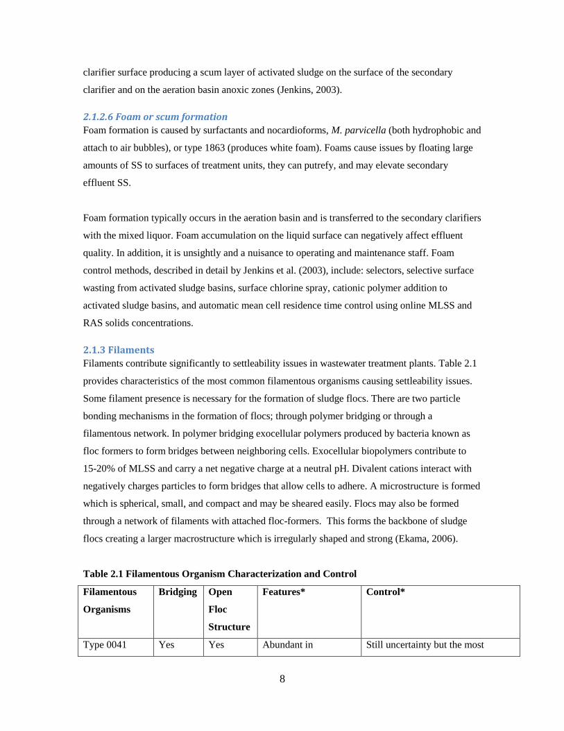
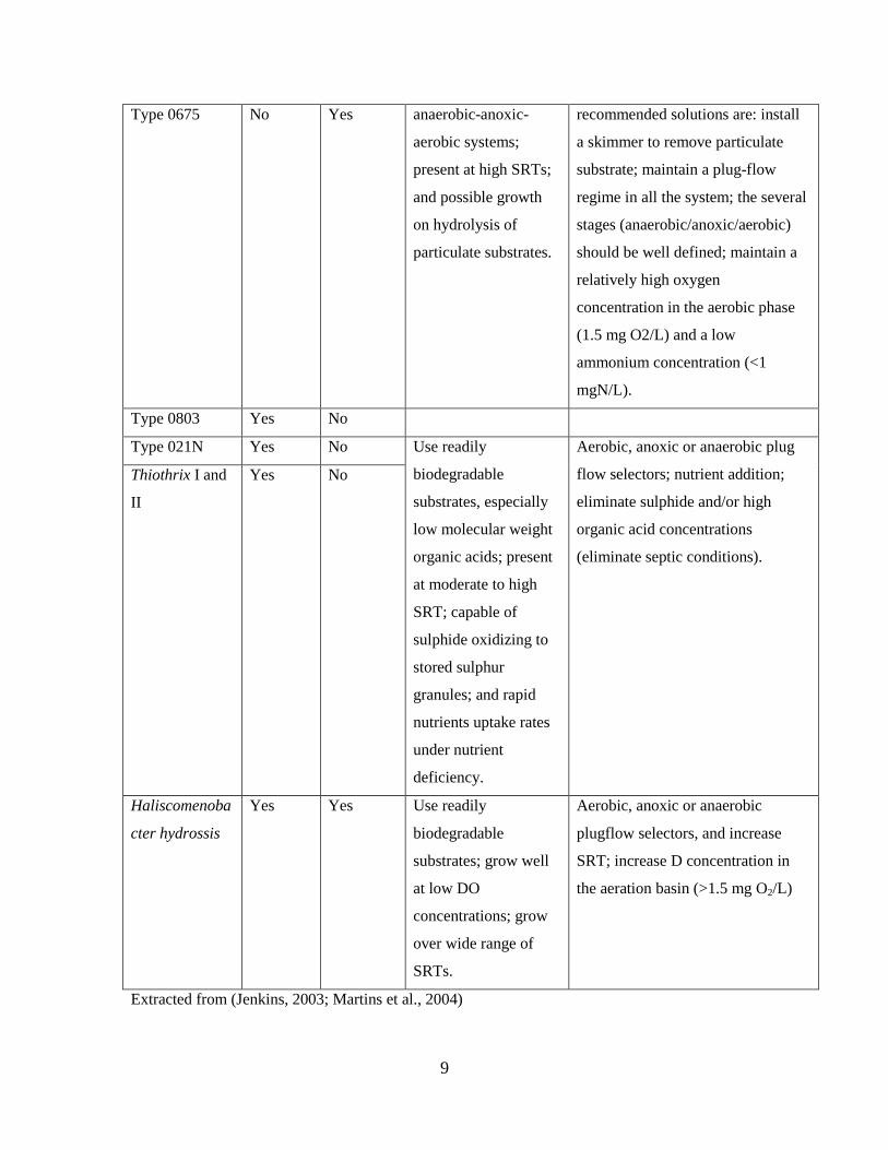
Filaments contribute significantly to settleability issues in wastewater treatment plants. Table 2.1
provides characteristics of the most common filamentous organisms causing settleability issues.
Some filament presence is necessary for the formation of sludge flocs. There are two particle
bonding mechanisms in the formation of flocs; through polymer bridging or through a
filamentous network. In polymer bridging exocellular polymers produced by bacteria known as
floc formers to form bridges between neighboring cells. Exocellular biopolymers contribute to
15-20% of MLSS and carry a net negative charge at a neutral pH. Divalent cations interact with
negatively charges particles to form bridges that allow cells to adhere. A microstructure is formed
which is spherical, small, and compact and may be sheared easily. Flocs may also be formed
through a network of filaments with attached floc-formers. This forms the backbone of sludge
flocs creating a larger macrostructure which is irregularly shaped and strong (Ekama, 2006).
Table 2.1 Filamentous Organism Characterization and Control
Filamentous
Organisms
Bridging Open
Floc
Structure
Features* Control*
Type 0041 Yes Yes Abundant in Still uncertainty but the most
9
Type 0675 No Yes anaerobic-anoxic-
aerobic systems;
present at high SRTs;
and possible growth
on hydrolysis of
particulate substrates.
recommended solutions are: install
a skimmer to remove particulate
substrate; maintain a plug-flow
regime in all the system; the several
stages (anaerobic/anoxic/aerobic)
should be well defined; maintain a
relatively high oxygen
concentration in the aerobic phase
(1.5 mg O2/L) and a low
ammonium concentration (<1
mgN/L).
Type 0803 Yes No
Type 021N Yes No Use readily
biodegradable
substrates, especially
low molecular weight
organic acids; present
at moderate to high
SRT; capable of
sulphide oxidizing to
stored sulphur
granules; and rapid
nutrients uptake rates
under nutrient
deficiency.
Aerobic, anoxic or anaerobic plug
flow selectors; nutrient addition;
eliminate sulphide and/or high
organic acid concentrations
(eliminate septic conditions).
Thiothrix I and
II
Yes No
Haliscomenoba
cter hydrossis
Yes Yes Use readily
biodegradable
substrates; grow well
at low DO
concentrations; grow
over wide range of
SRTs.
Aerobic, anoxic or anaerobic
plugflow selectors, and increase
SRT; increase D concentration in
the aeration basin (>1.5 mg O2/L)
Extracted from (Jenkins, 2003; Martins et al., 2004)
10
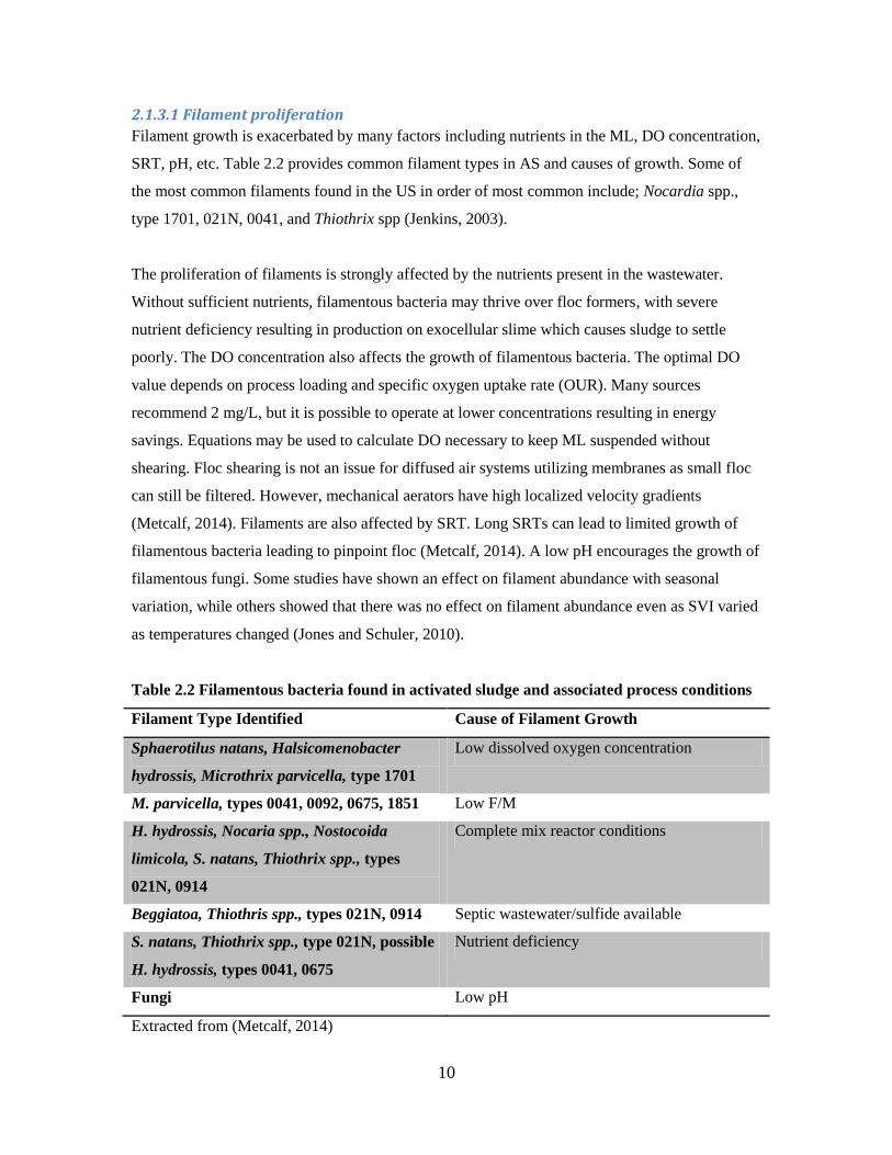
2.1.3.1 Filament proliferation
Filament growth is exacerbated by many factors including nutrients in the ML, DO concentration,
SRT, pH, etc. Table 2.2 provides common filament types in AS and causes of growth. Some of
the most common filaments found in the US in order of most common include; Nocardia spp.,
type 1701, 021N, 0041, and Thiothrix spp (Jenkins, 2003).
The proliferation of filaments is strongly affected by the nutrients present in the wastewater.
Without sufficient nutrients, filamentous bacteria may thrive over floc formers, with severe
nutrient deficiency resulting in production on exocellular slime which causes sludge to settle
poorly. The DO concentration also affects the growth of filamentous bacteria. The optimal DO
value depends on process loading and specific oxygen uptake rate (OUR). Many sources
recommend 2 mg/L, but it is possible to operate at lower concentrations resulting in energy
savings. Equations may be used to calculate DO necessary to keep ML suspended without
shearing. Floc shearing is not an issue for diffused air systems utilizing membranes as small floc
can still be filtered. However, mechanical aerators have high localized velocity gradients
(Metcalf, 2014). Filaments are also affected by SRT. Long SRTs can lead to limited growth of
filamentous bacteria leading to pinpoint floc (Metcalf, 2014). A low pH encourages the growth of
filamentous fungi. Some studies have shown an effect on filament abundance with seasonal
variation, while others showed that there was no effect on filament abundance even as SVI varied
as temperatures changed (Jones and Schuler, 2010).
Table 2.2 Filamentous bacteria found in activated sludge and associated process conditions
Filament Type Identified Cause of Filament Growth
Sphaerotilus natans, Halsicomenobacter
hydrossis, Microthrix parvicella, type 1701
Low dissolved oxygen concentration
M. parvicella, types 0041, 0092, 0675, 1851 Low F/M
H. hydrossis, Nocaria spp., Nostocoida
limicola, S. natans, Thiothrix spp., types
021N, 0914
Complete mix reactor conditions
Beggiatoa, Thiothris spp., types 021N, 0914 Septic wastewater/sulfide available
S. natans, Thiothrix spp., type 021N, possible
H. hydrossis, types 0041, 0675
Nutrient deficiency
Fungi Low pH
Extracted from (Metcalf, 2014)
11
2.1.3.2 DO
Low dissolved oxygen levels may lead to the growth of bulking organisms. Achieving the oxygen
demand profile needed is often done by tapered aeration or step-feed operation (WEF, 2005).
Because filamentous bacteria have the capability of growing outside the floc structure, they have
an advantage over floc-forming bacteria in diffusion-resistant environments. This allows
filaments to exist outside of the floc, giving them preferential access to the bulk liquid substrate
(Martins et al., 2004). Martins et al. (2004) compared floc growth with biofilm growth, finding
that low substrate or low oxygen concentrations lead to open, filamentous flocs resulting in poor
settling. Palm et al. (1980) found that the DO concentration required was a function of the F/M
ratio; as F/M increased, the DO required also increased. This could be remedied by manipulating
F/M and DO ratios, but this would take longer than the onset of bulking. A quick fix such as
chemical addition could be used if a rapid fix was necessary.
2.1.3.3 Filament Counting Methods and Characterization
Filaments may be counted by observing the amount of filament extending from a floc, by
counting the number of filaments intersecting a hairline on a slide cover, or may be counted
through Nocardioform filament organism counting where gram positive filaments are visible in a
gram stained ML sample (Jenkins, 2003). Floc and filamentous microorganism characterization is
useful in determining settling and compaction characteristics of AS. Floc characteristics worth
noting include; floc size, shape (round, irregular, compact, diffuse), protozoa and other
microorganisms, nonbiological organic and inorganic particles, bacterial colonies, cells dispersed
in bulk solution, and effects of filamentous organisms on floc structure. A scale from 0-6 is used
for filamentous organism abundance in a floc. In order to identify the filamentous organisms
present, a dichotomous key can be used by viewing the filament’s characteristics such as;
branching, motility, filament shape, location, attached bacteria, sheath, cross-walls, filament
width, filament length, cell shape, cell size, sulfur deposits, other granules, and staining reactions
(Jenkins, 2003). Once the filamentous organism has been identified, it is necessary to pinpoint
relationships between the filaments and the operational conditions present when they occur to
control for their growth.
2.1.4 Bulking Control
Care must be taken to control for excessive growth of filaments. It is important to understand the
cause of bulking in order to control it. Parameters to take into consideration are wastewater
characteristics, DO content, process loading as N and P in industrial wastes may lead to bulking,
internal plant overloading, and analyzing ML under a microscope for microbial growth or change
in floc structure (Grady, 2011). Filaments can be controlled permanently through types of
12
selectors, DO concentration, SRT, and nutrient addition. For temporary filament control, which is
generally cheaper than permanent solutions, chemical additions such as chlorine or hydrogen
peroxide may be used (Ekama, 2006).
2.1.4.1 Kinetic and Metabolic Selection
Filaments may be controlled through kinetic selection as filamentous bacteria and floc-forming
bacteria have separate growth strategies. Chudoba et al (1985) developed the kinetic selection
theory based on Monod kinetics to describe filamentous growth in AS. Filamentous bacteria can
be described as slow-growing k strategists, such as Sphaerotilus and Leucothrix coharens, while
floc-forming bacteria are described as r strategist where floc-formers grow faster when the
substrate concentration is high and filamentous bacteria grow faster when substrate concentration
is low (Grady, 2011). Filamentous bacteria have maximum growth rates (μmax) and affinity
constants (Ks) lower than floc-forming bacteria. Floc-formers out compete filamentous bacteria at
a certain concentration, so this concentration must be kept below this level so biomass formation
occurs (Grady, 2011). When the substrate concentration is low filamentous bacteria have a higher
substrate uptake rate than floc formers and consume more of the available substrate. When the
substrate concentration is high, the filamentous bacteria are suppressed since their growth rate is
below that of floc-forming bacteria. The kinetic selection theory gave rise to the selector reactor
to control filamentous bulking. Through kinetic selection, a substrate concentration gradient is
present throughout the bioreactor. This substrate gradient may be achieved in plug flow like
conditions. The concentration at the inlet will favor floc-formers over filamentous bacteria.
Filaments may persist over floc formers when readily biodegradable substrate is consistently
supplied at low concentrations. In some cases a substrate concentration gradient will form
granular floc particles with high settling rates. Chudoba deemed it necessary to keep a high
substrate concentration, S, to select for filamentous bacteria suppression. However, it has been
shown through application that bench scale experiments using selectors to control filamentous
bulking does not always translate to full-scale operation.
Filaments with a high affinity for biodegradable organic matter may also be controlled through
metabolic selection. This is done by eliminating DO as a terminal electron acceptor and either
adding nitrate to create anoxic conditions, or eliminating both to create anaerobic conditions.
Many floc formers can take up biodegradable organic matter under anoxic or anaerobic
conditions while many filamentous bacteria cannot (Metcalf, 2014).
13
2.1.4.2 Chemical Addition
Chemical addition can be used to enhance excess filaments or induce flocculation (WEF, 2005).
Chemical coagulants may induce flocculation, cationic polymers added at a concentration of <1
mg/L has been shown to improve mixed liquor settleability. RAS or sidestream chlorination can
reduce bulking sludge, although RAS chlorination may interfere with nitrification. Hydrogen
peroxide may be substituted for chlorine in many cases. Selection of inorganic salts, polymers, or
other flocculent aids can be used but should be based on laboratory studies (Grady, 2011).
2.1.5 Selectors
The selector was an activated sludge process first used in 1973 for selectively growing non-
filamentous organisms and inhibiting filamentous organisms. Selectors are split into three main
categories; aerobic, anoxic, and anaerobic, each providing certain advantages, outlined in Table
2.3.
In 1973 J. Chudoba defined selectors as the part of the aeration system with a substantial
concentration gradient of substrate (Chudoba, 1973). Chudoba’s 1973 study demonstrated that the
growth of filamentous microorganisms was effectively suppressed by means of a selector, with
soluble COD removal ranging from 90-95%. Once filamentous organisms were placed into a
system with a higher concentration gradient, they gradually decreased, but often at a slow rate. It
was found that the period needed to attain steady state composition of the mixed culture depended
on the original composition of the mixed culture and the concentration gradient of the substrate
along the system.
The authors of a 1997 full-scale evaluation of factors affecting the performance of anoxic
selectors concluded that both aerobic and anoxic SRTs have more significance when minimizing
the growth of filamentous organisms than does the organic loading (F/M) (Parker, 1998). It is still
desirable to maintain a high F/M in the initial contact zone to achieve rapid soluble organic matter
uptake rates. Although a single selector tank can be effective in controlling filaments, multiple
compartments maintaining plug-flow enhance substrate gradient and improve kinetic selection.
14
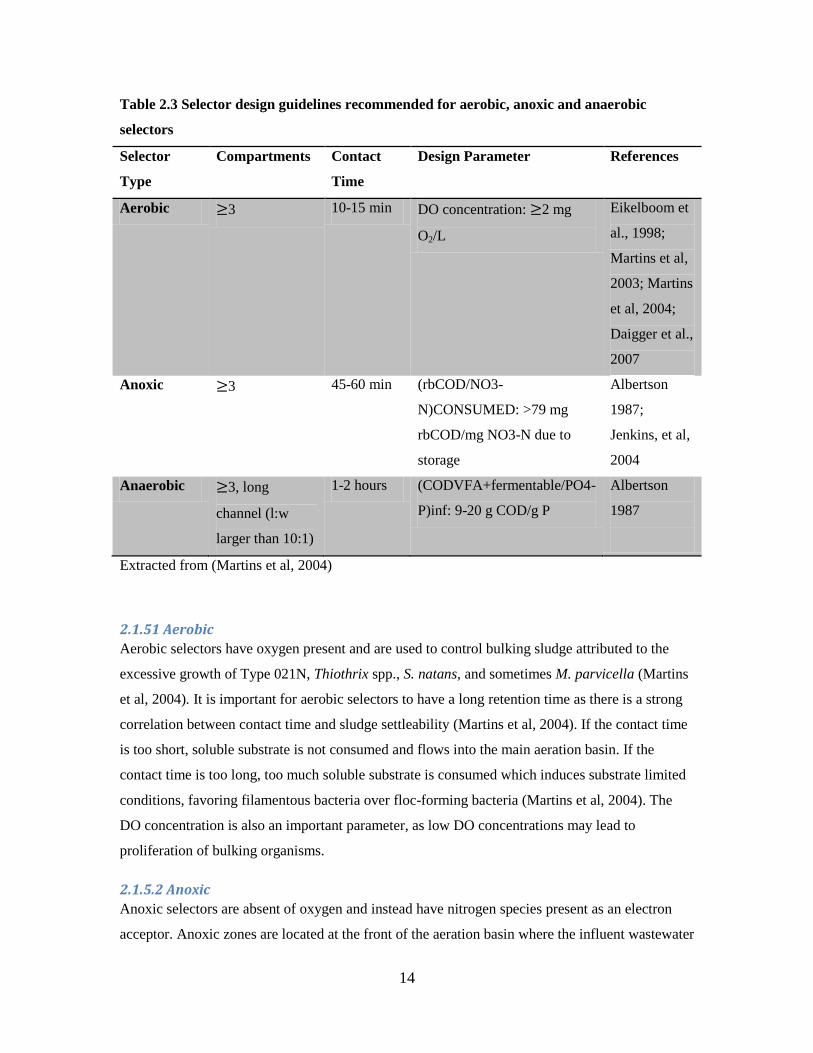
Table 2.3 Selector design guidelines recommended for aerobic, anoxic and anaerobic
selectors
Selector
Type
Compartments Contact
Time
Design Parameter References
Aerobic 3 10-15 min DO concentration: 2 mg
O2/L
Eikelboom et
al., 1998;
Martins et al,
2003; Martins
et al, 2004;
Daigger et al.,
2007
Anoxic 3 45-60 min (rbCOD/NO3-
N)CONSUMED: >79 mg
rbCOD/mg NO3-N due to
storage
Albertson
1987;
Jenkins, et al,
2004
Anaerobic 3, long
channel (l:w
larger than 10:1)
1-2 hours (CODVFA+fermentable/PO4-
P)inf: 9-20 g COD/g P
Albertson
1987
Extracted from (Martins et al, 2004)
2.1.51 Aerobic
Aerobic selectors have oxygen present and are used to control bulking sludge attributed to the
excessive growth of Type 021N, Thiothrix spp., S. natans, and sometimes M. parvicella (Martins
et al, 2004). It is important for aerobic selectors to have a long retention time as there is a strong
correlation between contact time and sludge settleability (Martins et al, 2004). If the contact time
is too short, soluble substrate is not consumed and flows into the main aeration basin. If the
contact time is too long, too much soluble substrate is consumed which induces substrate limited
conditions, favoring filamentous bacteria over floc-forming bacteria (Martins et al, 2004). The
DO concentration is also an important parameter, as low DO concentrations may lead to
proliferation of bulking organisms.
2.1.5.2 Anoxic
Anoxic selectors are absent of oxygen and instead have nitrogen species present as an electron
acceptor. Anoxic zones are located at the front of the aeration basin where the influent wastewater
15
and RAS mix. This is achieved through a RAS line being fed into the anoxic zone, supplying
nitrate-rich wastewater. Soluble substrate is consumed in anoxic selectors, selecting against
filamentous bacteria before entering the aerobic phase. Too much rbCOD entering the aerobic
phase because of limited storage capacity in the anoxic phase may result in bulking sludge. The
main design parameter for anoxic selectors is the rbCOD/NO3-N (readily biodegradable chemical
oxygen demand/nitrate) ratio. It can be difficult to determine this ratio as some denitrification
takes place in the secondary clarifier, resulting in periods with lower nitrate concentrations or
possibly even anaerobic conditions (Martins et al, 2004).
2.1.5.3 Anaerobic
Anaerobic selectors contain no oxygen or oxidized nitrogen species. In an anaerobic selector, it is
desired for the rbCOD to be consumed before the aerobic phase. The main design parameter is
the ratio of rbCOD uptake rate to phosphorus release rate. In anaerobic selectors, PAO and GAO
are able to store substrate, allowing them to remove the incoming organic load. As the PAOs and
GAOs consume more, there is less substrate available in the aerobic stage allowing for improved
sludge settleability.
2.1.6 Classifying Selectors
A classifying selector is a physical mechanism by which nuisance organisms (foam-causing) are
selected against (Parker, 2003). In 1987 Pretorius and Laubscher proposed a method for wasting
foam-causing organisms based on their physical properties by using aeration to waste them at the
surface of a “flotation cell” which became the basis for developing classifying selectors (Parker,
2003). The term classifying selector was coined by Brown and Caldwell in the 1990s. Nuisance
organisms are an issue for wastewater treatment plants, especially when operating at high SRTs.
Foam causing organisms will remain at the surface of a tank remaining in the tank for longer than
the ML, or will be wasted into the effluent which is undesired unless continuous surface wasting
through an external selector is applied. A classifying selector works by selectively wasting the
foam layer accumulating on the surface in an aeration basin. In certain plants Nocardia filament
trapping is often an issue and it is difficult to control Nocardia proliferation through any method,
which was the case for an oxygen activated sludge plant in a 1996 study which split the plant in
half and applied classifying selectors to the end of the aeration basin on one side and on the RAS
line in the other. It was found that the side with the classifying selector applied to the aeration
basin was more effective at controlling foam than the one applied to the RAS line and that
Nocardia levels has been reduced by 30% (Pagilla et al, 1996). The optimum approach to
reducing nuisance organisms has been found to be continuous surface wasting regardless of foam
16
levels. The benefits of a classifying selector allow for not only eliminating nuisance conditions
but also reducing foam causing organisms, preventing them from proliferating downstream
processes.
2.2 Biological Phosphorus Removal
2.2.1 Background
Phosphorus can be removed through enhanced biological phosphorus removal (EBPR) in which
microorganisms called PAO exist in the solids which consume phosphorus. Phosphorus may also
be removed through chemical phosphorus removal to form a precipitate. This is used as an
effluent polishing step, to prevent struvite formation, or to supplement EBPR. Ferric is a common
chemical often applied before the primary and/or secondary clarifier to bind the phosphorus
which can then be settled out. Chemical addition to primary clarifiers is also used to remove
phosphorus for nutrient control, heavy metals to meet toxicity requirements, and hydrogen sulfide
to lower odor emissions (WEF, 2005).
In both of these methods, phosphorus is contained in a solid form and is then settled in a clarifier
and removed in sludge wasting. EBPR has been used for decades and allows for plants to reach
effluent standards while minimizing chemical consumption and sludge production (Metcalf,
2014; Neethling et al, 2005). EBPR consists of alternating anaerobic and aerobic zones where
organic uptake and P release occur under anaerobic conditions and P uptake occurs under aerobic
or anoxic conditions. The initial anaerobic selector allows for the enrichment of the bacteria that
take up P in aerobic conditions. Many factors affect the performance of EBPR, such as; influent
wastewater characteristics, nitrogen removal requirements, presence of nitrate, management of
return flow from anaerobic solids processing steps, chemical addition for phosphorus polishing,
and other processes used to enhance EBPR (Neethling, 2005). IFAS installation could also
improve EBPR as it allows for a short SRT in the suspended growth which favors biomass
phosphorus accumulation (Sriwiriyarat and Randall, 2005). Some issues utilizing IFAS for EBPR
include the low biomass MCRTs, and low temperatures resulting in washout and lack of an
anaerobic selector in most plants utilizing BNR. A 2005 study implemented IFAS media into
anoxic selectors only, aerobic selectors only, and both anoxic and aerobic selectors, finding that
each one of these was a viable method for EBPR. However, the control system utilized COD
more efficiently than the IFAS systems. EBPR performance was reduced in systems that split the
influent flow between aerobic and anoxic zones for enhancing denitrification because the rbCOD
present in the anoxic zone caused the biofilms on the media to release phosphorus, which was not
17
then sent to the aerobic phase to take up the released phosphorus. The performance was found to
be similar in the IFAS systems and conventional BNR systems under the same type of operation
(Sriwiriyarat and Randall, 2005).
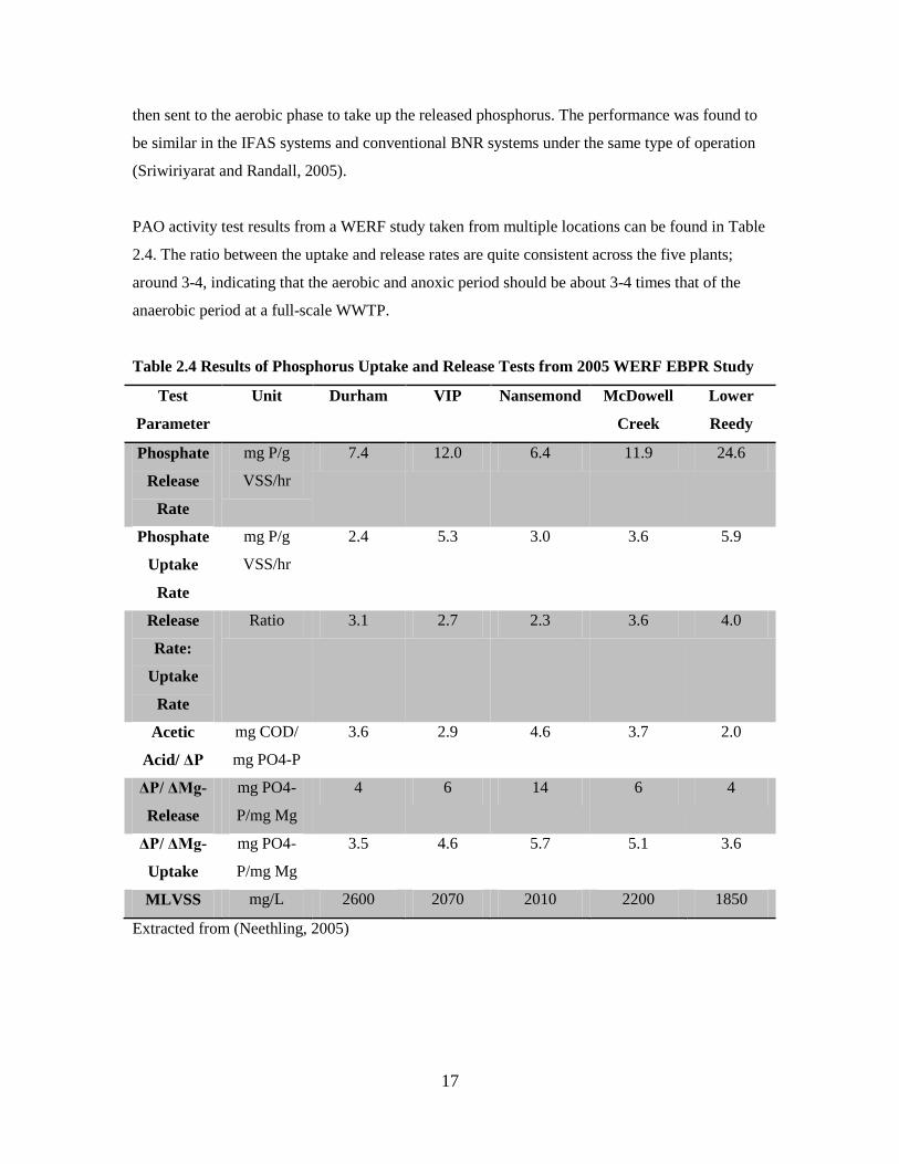
PAO activity test results from a WERF study taken from multiple locations can be found in Table
2.4. The ratio between the uptake and release rates are quite consistent across the five plants;
around 3-4, indicating that the aerobic and anoxic period should be about 3-4 times that of the
anaerobic period at a full-scale WWTP.
Table 2.4 Results of Phosphorus Uptake and Release Tests from 2005 WERF EBPR Study
Test
Parameter
Unit Durham VIP Nansemond McDowell
Creek
Lower
Reedy
Phosphate
Release
Rate
mg P/g
VSS/hr
7.4 12.0 6.4 11.9 24.6
Phosphate
Uptake
Rate
mg P/g
VSS/hr
2.4 5.3 3.0 3.6 5.9
Release
Rate:
Uptake
Rate
Ratio 3.1 2.7 2.3 3.6 4.0
Acetic
Acid/ ΔP
mg COD/
mg PO4-P
3.6 2.9 4.6 3.7 2.0
ΔP/ ΔMg-
Release
mg PO4-
P/mg Mg
4 6 14 6 4
ΔP/ ΔMg-
Uptake
mg PO4-
P/mg Mg
3.5 4.6 5.7 5.1 3.6
MLVSS mg/L 2600 2070 2010 2200 1850
Extracted from (Neethling, 2005)
18
2.2.2 PAO, DPAO and GAO metabolism
2.2.2.1 PAO
PAO are heterotrophic bacteria that take up phosphorus in aerobic conditions and are critical for
EBPR performance. PAO may provide over 80% biological phosphorus removal (Metcalf, 2014).
The anaerobic zone provides for the fermentation of the influent rbCOD to acetate. (Metcalf,
2014). PAO are able to outcompete ordinary heterotrophic bacteria, as they have the ability to
accumulate volatile fatty acids (VFAs) in their cells in the absence of an electron acceptor. Other
heterotrophic bacteria are not able to uptake acetate and starve while the PAO use COD in the
anaerobic zone (Metcalf, 2014). Under anaerobic conditions, PAO consume acetic and propionic
acid and use stored polyphosphates as energy to assimilate acetate and produce intracellular poly-
β-hydroxyalkanoate (PHA). The energy for this transport and storage reaction is thought to be
supplied by the hydrolysis of the intracellular polyphosphate to phosphate, which is released from
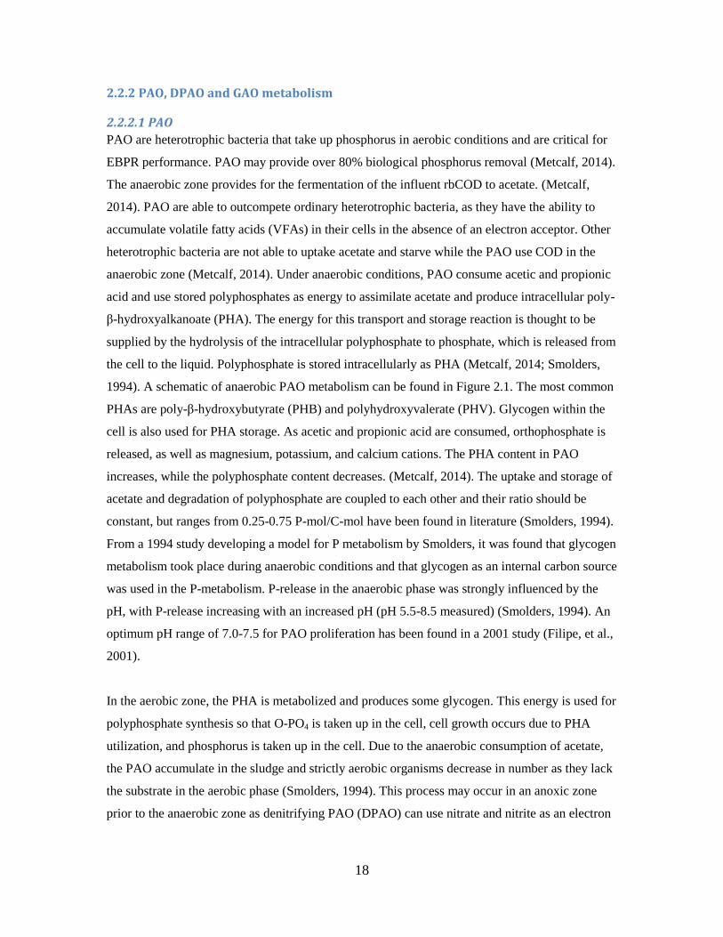
the cell to the liquid. Polyphosphate is stored intracellularly as PHA (Metcalf, 2014; Smolders,
1994). A schematic of anaerobic PAO metabolism can be found in Figure 2.1. The most common
PHAs are poly-β-hydroxybutyrate (PHB) and polyhydroxyvalerate (PHV). Glycogen within the
cell is also used for PHA storage. As acetic and propionic acid are consumed, orthophosphate is
released, as well as magnesium, potassium, and calcium cations. The PHA content in PAO
increases, while the polyphosphate content decreases. (Metcalf, 2014). The uptake and storage of
acetate and degradation of polyphosphate are coupled to each other and their ratio should be
constant, but ranges from 0.25-0.75 P-mol/C-mol have been found in literature (Smolders, 1994).
From a 1994 study developing a model for P metabolism by Smolders, it was found that glycogen
metabolism took place during anaerobic conditions and that glycogen as an internal carbon source
was used in the P-metabolism. P-release in the anaerobic phase was strongly influenced by the
pH, with P-release increasing with an increased pH (pH 5.5-8.5 measured) (Smolders, 1994). An
optimum pH range of 7.0-7.5 for PAO proliferation has been found in a 2001 study (Filipe, et al.,
2001).
In the aerobic zone, the PHA is metabolized and produces some glycogen. This energy is used for
polyphosphate synthesis so that O-PO4 is taken up in the cell, cell growth occurs due to PHA
utilization, and phosphorus is taken up in the cell. Due to the anaerobic consumption of acetate,
the PAO accumulate in the sludge and strictly aerobic organisms decrease in number as they lack
the substrate in the aerobic phase (Smolders, 1994). This process may occur in an anoxic zone
prior to the anaerobic zone as denitrifying PAO (DPAO) can use nitrate and nitrite as an electron
19
acceptor for substrate oxidation (Metcalf, 2014). A schematic of PAO metabolism under
aerobic/anoxic conditions can be found on the right side of Figure 2.1.
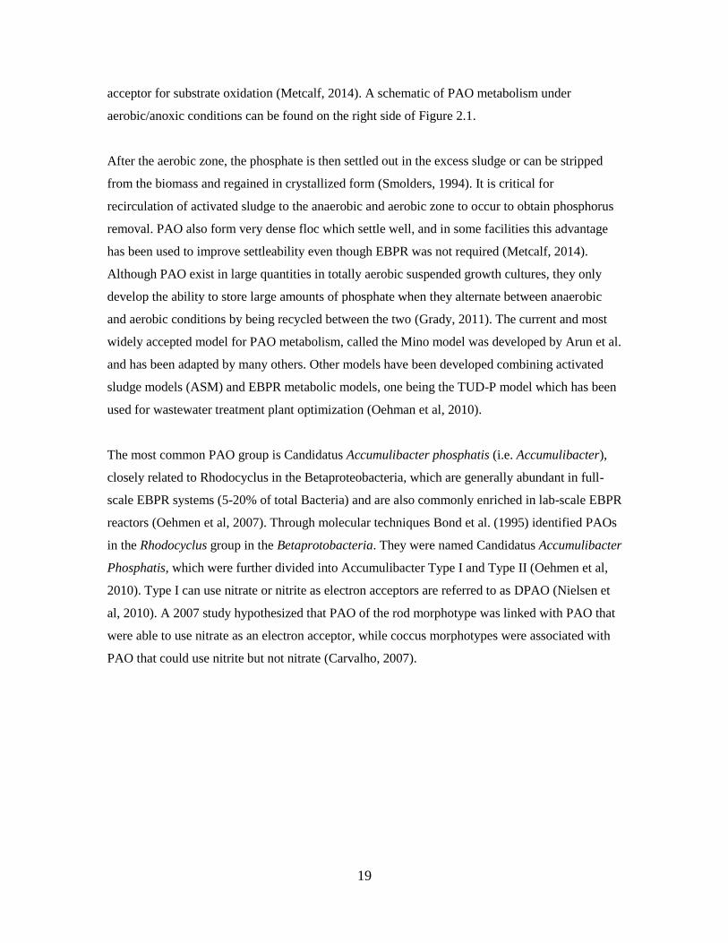
After the aerobic zone, the phosphate is then settled out in the excess sludge or can be stripped
from the biomass and regained in crystallized form (Smolders, 1994). It is critical for
recirculation of activated sludge to the anaerobic and aerobic zone to occur to obtain phosphorus
removal. PAO also form very dense floc which settle well, and in some facilities this advantage
has been used to improve settleability even though EBPR was not required (Metcalf, 2014).
Although PAO exist in large quantities in totally aerobic suspended growth cultures, they only
develop the ability to store large amounts of phosphate when they alternate between anaerobic
and aerobic conditions by being recycled between the two (Grady, 2011). The current and most
widely accepted model for PAO metabolism, called the Mino model was developed by Arun et al.
and has been adapted by many others. Other models have been developed combining activated
sludge models (ASM) and EBPR metabolic models, one being the TUD-P model which has been
used for wastewater treatment plant optimization (Oehman et al, 2010).
The most common PAO group is Candidatus Accumulibacter phosphatis (i.e. Accumulibacter),
closely related to Rhodocyclus in the Betaproteobacteria, which are generally abundant in full-
scale EBPR systems (5-20% of total Bacteria) and are also commonly enriched in lab-scale EBPR
reactors (Oehmen et al, 2007). Through molecular techniques Bond et al. (1995) identified PAOs
in the Rhodocyclus group in the Betaprotobacteria. They were named Candidatus Accumulibacter
Phosphatis, which were further divided into Accumulibacter Type I and Type II (Oehmen et al,
2010). Type I can use nitrate or nitrite as electron acceptors are referred to as DPAO (Nielsen et
al, 2010). A 2007 study hypothesized that PAO of the rod morphotype was linked with PAO that
were able to use nitrate as an electron acceptor, while coccus morphotypes were associated with
PAO that could use nitrite but not nitrate (Carvalho, 2007).

20
Figure 2.1 PAO metabolism under anaerobic and aerobic/anoxic conditions.
2.2.2.2 GAO
GAOs were originally referred to as “G” bacteria because of their growth and glycogen storage
with glucose feed. The term GAO (Mino et al, 1995) is based on the organism’s storage of
glycogen under aerobic conditions and consumption of glycogen under anaerobic conditions to
provide energy for VFA uptake and production of PHA in the anaerobic zone of an EBPR system
(Metcalf, 2014). GAO compete with PAO for substrate, and do not remove any phosphorus from
the system. In addition to GAO, many other organisms may compete with PAO for substrate.
GAOs use glycolysis to obtain energy and reducing equivalents for VFA uptake and PHA
storage. Under aerobic conditions, glycogen is regenerated from PHAs (Acevedo et al, 2014).
PAO and GAO were thought to be different organisms, but recent studies have shown PAO are
able to act like GAO under certain conditions (Acevedo et al, 2014). A 2014 study by Acevedo
generated a new model to include PAO which altered their metabolism to act like GAO under low
phosphorus concentrations.
GAO belong to the phenotype Gammaproteobacteria and were named “Candidatus
Competibacter Phosphatis” by Crocetti et al (2002). All GAOs identified so far have been able to
use nitrate and an electron acceptor in addition to oxygen, but only Competibacter Type I can use
nitrite as well. (Nielsen et al, 2010.)
Anaerobic Aerobic /Anoxic
VFA
PHB Glycogen
Poly-P
PHB
Glycogen
ATP
PO43-
New
Cellmass
Poly-P
ATP
PO43-
21
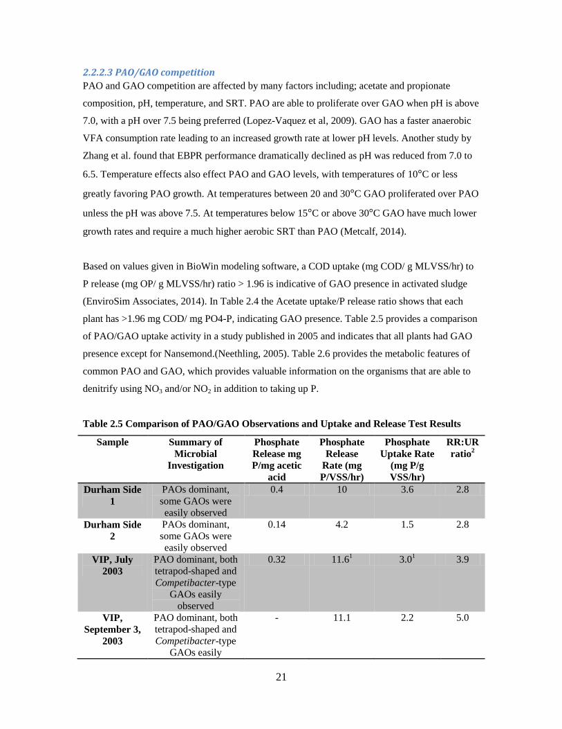
2.2.2.3 PAO/GAO competition
PAO and GAO competition are affected by many factors including; acetate and propionate
composition, pH, temperature, and SRT. PAO are able to proliferate over GAO when pH is above
7.0, with a pH over 7.5 being preferred (Lopez-Vaquez et al, 2009). GAO has a faster anaerobic
VFA consumption rate leading to an increased growth rate at lower pH levels. Another study by
Zhang et al. found that EBPR performance dramatically declined as pH was reduced from 7.0 to
6.5. Temperature effects also effect PAO and GAO levels, with temperatures of 10 C or less
greatly favoring PAO growth. At temperatures between 20 and 30 C GAO proliferated over PAO
unless the pH was above 7.5. At temperatures below 15 C or above 30 C GAO have much lower
growth rates and require a much higher aerobic SRT than PAO (Metcalf, 2014).
Based on values given in BioWin modeling software, a COD uptake (mg COD/ g MLVSS/hr) to
P release (mg OP/ g MLVSS/hr) ratio > 1.96 is indicative of GAO presence in activated sludge
(EnviroSim Associates, 2014). In Table 2.4 the Acetate uptake/P release ratio shows that each
plant has >1.96 mg COD/ mg PO4-P, indicating GAO presence. Table 2.5 provides a comparison
of PAO/GAO uptake activity in a study published in 2005 and indicates that all plants had GAO
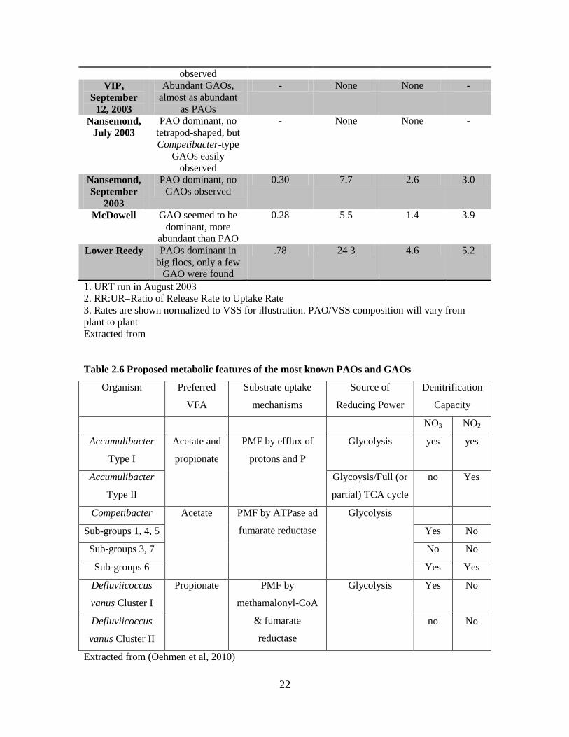
presence except for Nansemond.(Neethling, 2005). Table 2.6 provides the metabolic features of
common PAO and GAO, which provides valuable information on the organisms that are able to
denitrify using NO3 and/or NO2 in addition to taking up P.
Table 2.5 Comparison of PAO/GAO Observations and Uptake and Release Test Results
Sample Summary of
Microbial
Investigation
Phosphate
Release mg
P/mg acetic
acid
Phosphate
Release
Rate (mg
P/VSS/hr)
Phosphate
Uptake Rate
(mg P/g
VSS/hr)
RR:UR
ratio2
Durham Side
1
PAOs dominant,
some GAOs were
easily observed
0.4 10 3.6 2.8
Durham Side
2
PAOs dominant,
some GAOs were
easily observed
0.14 4.2 1.5 2.8
VIP, July
2003
PAO dominant, both
tetrapod-shaped and
Competibacter-type
GAOs easily
observed
0.32 11.61 3.0
1 3.9
VIP,
September 3,
2003
PAO dominant, both
tetrapod-shaped and
Competibacter-type
GAOs easily
- 11.1 2.2 5.0
22
observed
VIP,
September
12, 2003
Abundant GAOs,
almost as abundant
as PAOs
- None None -
Nansemond,
July 2003
PAO dominant, no
tetrapod-shaped, but
Competibacter-type
GAOs easily
observed
- None None -
Nansemond,
September
2003
PAO dominant, no
GAOs observed
0.30 7.7 2.6 3.0
McDowell GAO seemed to be
dominant, more
abundant than PAO
0.28 5.5 1.4 3.9
Lower Reedy PAOs dominant in
big flocs, only a few
GAO were found
.78 24.3 4.6 5.2
1. URT run in August 2003
2. RR:UR=Ratio of Release Rate to Uptake Rate
3. Rates are shown normalized to VSS for illustration. PAO/VSS composition will vary from
plant to plant
Extracted from
Table 2.6 Proposed metabolic features of the most known PAOs and GAOs
Organism Preferred
VFA
Substrate uptake
mechanisms
Source of
Reducing Power
Denitrification
Capacity
NO3 NO2
Accumulibacter
Type I
Acetate and
propionate
PMF by efflux of
protons and P
Glycolysis yes yes
Accumulibacter
Type II
Glycoysis/Full (or
partial) TCA cycle
no Yes
Competibacter Acetate PMF by ATPase ad
fumarate reductase
Glycolysis
Sub-groups 1, 4, 5 Yes No
Sub-groups 3, 7 No No
Sub-groups 6 Yes Yes
Defluviicoccus
vanus Cluster I
Propionate PMF by
methamalonyl-CoA
& fumarate
reductase
Glycolysis Yes No
Defluviicoccus
vanus Cluster II
no No
Extracted from (Oehmen et al, 2010)
23
2.2.2.4 DPAO
Some PAO species can use nitrate and nitrite as an electron acceptor for substrate oxidation
(Metcalf, 2014). These organisms are celled Denitrifying PAO, or DPAO, and have the ability to
remove nitrogen and phosphorus simultaneously. Some recent studies have focused on the
development of simultaneous nitrification, denitrification and P removal processes, sometimes
using granular sludge (Oehmen et al, 2007). The results from a 2010 study by Oehmen et al, in
combination with previous studies, strongly suggest that DPAOs and PAOs are different
microorganisms, whereby Accumulibacter Type I are likely to be able to reduce nitrate and
Accumulibacter Type II are not likely to be able to reduce nitrate (Oehmen et al, 2010). An
advantage to having DPAO in a BNR process is that the use of nitrate rather than oxygen as the
electron acceptor leads to slightly less sludge production and a more efficient use of COD as it is
used for phosphorus uptake and denitrification simultaneously (Ahn, 2002). Kuba et al (1996)
developed a two sludge system with nitrifiers in one and DPAO in another where supernatant
from the nitrifer system fed nitrate to the DPAO. Conventionally an aerobic step is needed for
nitrification to supply nitrate as an electron acceptor for PAO. This results in large amounts of
PHB being aerobically oxidized by PAO in long aerobic periods resulting in less COD available
for denitrification. By skipping this nitrification step, it was found that 15 mg P/l and 105 mg N/l
were removed using only 400 mg COD/l HAc. Calculations proved that the sludge production
required COD was 30% and 50% less than conventional phosphorus and nitrogen removal
systems, respectively. A study was performed on phosphorus activity in three separate reactors
with different electron acceptors; one with only oxygen, one with oxygen and nitrate, and one
with only nitrate. The reactor using oxygen and nitrate had the highest phosphorus uptake rates,
indicating a presence of DPAO that could utilize nitrate under aerobic conditions, while the
reactor with only nitrate had a decreasing phosphorus uptake over time (Ahn, 2002).
2.2.3 Conditions favoring EBPR
EBPR performance strongly relies on the bacteria population, which varies depending on factors
such as pH, temperature, influent characteristics, and SRT. Conditions found to favor EBPR and
achieve consistent low effluent phosphate concentrations include: high influent BOD:TP,
exclusion of oxidants (nitrate and DO) from anaerobic zone, excluding or minimizing recycle
flows and loads fluctuations from solids processing, favorable operation conditions (low SRT,
modest temperature, sufficient DO in aeration basin, balanced anaerobic and aerobic HRTs)
(Neethling, 2005). A high SRT may lead to a larger portion of the PAO population being lost to
endogenous decay, reducing the PAO in the waste sludge (Whang and Park, 2002). EBPR
24
systems have shown decreased EBPR activity rates and lower temperatures (Brdjanovic, 1998).
Some EBPR has achieved good performance at lower temperatures but a higher sludge age is
needed as the process kinetics decrease at lower temperatures. Brdyanovic found that as the
temperature decreased from 20°C to 10°C, incomplete phosphorus uptake occurred and that only
15% of acetate was consumed in the anaerobic zone and the rest was consumed in the aerobic
zone. The result was a high phosphorus concentration in the effluent and a washout of PAO.
However, an increase in SRT, the system gradually recovered (Brdjanovic, 1998) Similar trends
were seen when the temperature was decreased to 5°C, with the system recovering when the SRT
was increased further.
A WERF study conducted in 2010 collecting plant data from 47 facilities through the U.S. found
that plants achieving the highest percentage of influent phosphorus removal supplement EBPR by
adding volatile fatty acids (VFAs) or by polishing with iron or aluminum containing chemicals
(Neethling, 2005). It was also found that two thirds of the facilities meeting effluent TP levels
lower than 0.5 mg/L did not have solids recycle streams from the dewatering of anaerobically
digested sludge. No correlation was found with TP removal and SRT. The maximum TP removal
for facilities with no VFA or chemical addition is 95%, with effluent TP concentrations ranging
from 0.2-2.0 mg/L.
Temperature impacts EBPR as it relates to VFA generation in the aerobic zone (Stensel, 1991).
The microbiology of the activated sludge is also impacted by temperature, including PAO.
Studies at warm-weather BNR plants showed temperatures exceeding 30°C compromised EBPR
efficiency, possibly because PAO growth rate was reduced and GAO proliferate at higher
temperatures (Neethling, 2005). This results in leftover substrate not consumed by PAO to enter
the aerobic zone, resulting in possible filament growth. Temperatures above 20°C have been
shown to favor GAO proliferation.
In the Neethling (2005) study, a correlation was found between the ratio of the uptake HRT to
release HRT and the observed performance rating, which was based on the conditions listed
above. The ratio between the uptake rate and release rate are extremely consistent, typically
between three and four based on release rate: uptake rate. This implies that in full scale treatment,
the aerobic contact time should be three to four times as long as the release time (anaerobic plus
excess-anoxic time) (Neethling, 2005).
25
2.2.3.1 Low Organic Loading
Under conditions of low total organic loading, the maintenance processes of PAOs and GAOs are
pushed to their limit since both organisms are put under conditions of no external carbon sources
for extended periods (Carvalheria et al, 2014). This causes them to deplete their internal carbon
and energy sources: PHAs and glycogen, as well as polyphosphate in the case of PAOs. This
study found that the biomass decay rate of GAOs was about 4 times higher than PAOs, showing
that PAOs are better adapted to survive in low carbon loading conditions. In the aerobic phase
PAOs tended to maintain a PHA reserve, while GAOs exhausted all of their PHA, which may
have contributed to their increased biomass decay rate (Carvalheria et al, 2014). Tu and Schuler
(2013) studied the effect of lowering the acetate concentration in an EBPR system through
decreasing the feeding rate, while maintaining the total acetate load to the bioreactor (i.e., 200 mg
COD/L per cycle). They similarly found that PAOs were able to flourish over GAOs under low
loading rates.
2.2.3.2 DO
Narayanan (2006) found that DO concentrations >2 mg/L in the initial aerobic zone resulted in
OP effluent values <0.05 mg/L while DO concentrations <2 mg/L led to variable yet increasing
effluent OP values. It was also found that EBPR upsets were due to disruption of the aerobic
uptake and not due to initial P release in the anaerobic phase, indicating that the initial aerobic
uptake phase is critical (Narayanan, 2006). This may be because the P uptake rate is highest when
the PHA content is highest. As PHA is constantly being used as an energy source in the aerobic
zone, the initial PHA concentration would be highest during the initial aerobic zone, and
therefore, this is where the P uptake rate would be highest and would decrease through further
aerobic zones. It is critical to maintain a high DO concentration in the initial aerobic zone,
ensuring it does not drop below 1.5 mg/L (Narayanan, 2006).
However, Narayanan (2006) did not take into account GAO. In a 2014 study by Carvalho et al.
the effect of aeration on the competition between PAOs and GAOs was investigated. Batch tests
of enriched PAO and GAO cultures were performed at different DO levels in the aerobic zone, in
order to determine how the aerobic kinetics of each population varies as a function of the DO
concentration. Long term tests were also administered to observe the microbial population
performance on each system at different DO levels. The study found that PAO thrive in low DO
levels in the aerobic zone, while high DO levels led to higher growth and activity of GAO. PAO
possess a higher affinity for oxygen and show a clear kinetic advantage over GAO at low DO
concentrations. The impact of aerobic HRT on the microbial population and EBPR performance
26
was also investigated, with results indicating a high aerobic HRT promoted the growth of GAO
over PAO. Incorporation of the oxygen affinity of PAOs and GAOs into WWTP models could be
highly useful to optimize EBPR processes (Carvalheria et al, 2014). A low HRT aerobic period
with low DO levels is optimal for PAO proliferation, which is beneficial as estimates of aeration
requirements in WWTP correspond to 45-75% of energetic costs (Rosso et al, 2008).
2.2.4 Processes
Reactors need to be designed to provide PAO with a competitive advantage over other bacteria.
This is done by utilizing an initial anaerobic selector (Metcalf, 2014). An anaerobic environment
allows for PAO to transport and consume influent rbCOD in the form of VFAs by using energy
made available from their stored phosphorus and polyphosphates. Other heterotrophic bacteria
cannot consume the rbCOD because the need an electron donor such as oxygen, nitrate, or nitrite
for oxidation-reduction reactions. PAO can then use their stored energy along with cellular
glycogen to direct the substrate uptake to internal carbohydrate storage products for oxidation
later in the aerobic zone (Metcalf, 2014).
The contents of the anaerobic tank are thoroughly mixed to provide contact with the return
activated sludge (RAS) and influent wastewater, and will have an HRT of 0.5-1.0 hour. SRT
values in the aerobic tank may range from 3-40 days (Metcalf, 2014). Conventionally bio-p
removal is established at high total SRTs (3-15 days) to retain PAOs. However, longer SRTs
allow for GAO to compete with PAO for carbon substrates. Competition between PAO and GAO
is also affected by the DO concentration and HRT. At low DO levels, Accumulibacter PAO have
an advantage over GAO. An increase of the aerobic HRT when the do is at 2 mg/L promoted
proliferation of GAO over PAO as found in a 2014 study by Carvalheria et al.
2.3 Granular Sludge
2.3.1 Background
Granular sludge is well understood in anaerobic processes, while aerobic granular sludge has not
yet been well researched. Granular sludge was first found in an upflow anaerobic sludge blanket
(UASB) at the end of the 1970s (Lettinga et al, 1980). Since the 1980s, granular sludge has been
used extensively in full-scale anaerobic reactors. Aerobic granular sludge was first discovered in
an upflow sludge blanket reactor in 1991 (Mishima and Nakamura, 1991). In 1997 a sequencing
batch reactor (SBR) was used to develop aerobic granular sludge and has been shown to be the
preferred reactor for aerobic granule formation as oppose to a UASB for anaerobic granular

27
sludge (Gao et al, 2011). Most research on aerobic granules has been done using an SBR and
focuses on cultivation conditions, factors influencing granulation, and the microbial community.
In 2005, aerobic granules were defined by the International Water Association (IWA) as
aggregates of microbial origin, which do not coagulate under reduced hydrodynamic shear, and
which settle significantly faster than activated sludge flocs (Gao et al, 2011). Aerobic granular
sludge is advantageous over sludge in floc form in that aerobic granules have a high biomass
retention when compared to flocculent sludge because of their high density and compact
structure; allowing a reactor to treat wastewater at a higher volumetric loading rate. They also
have a high settling velocity which can reach 50-90 m/h depending on the size and density (Gao
et al, 2011). Various wastewaters and shock loadings are both treatable using aerobic granular
sludge (Gao et al, 2011). No sludge bulking has been observed in aerobic granular sludge.
Granular sludge is unique to conventional sludge in the there is no need for separate aerobic and
anaerobic selectors; all processes occur in different layers within the granular biomass, there will
be segregation of bacteria as a function of depth within the granules. A stratification of layers
exists within granules as nitrifiers are located in layers receiving oxygen penetration and
denitrifiers and PAO are present in the inner anoxic layers. A 2013 study found that the outer
layers are subjected to more shear stress and that high biomass retention selects for slow growing
organisms (Winkler et al, 2013).
2.3.2 Settleability
Aerobic granules have a high density and a high biomass retention capacity which directly relates
to the settleability of sludge and solids liquid separation in the reactor (Gao, et al., 2011). Various
studies showed the settling of aerobic granules to vary between 18-90 m/h with some even
reaching 130 m/h, which are similar for anaerobic granules, but much higher than activate sludge
which range from 7-10 m/h. The SVI of aerobic granules is generally below 80 mL/g and can
even get as low as 20 mL/g. A settling model for aerobic granules was developed by Lui et al in
2005 showing that the settling velocity was a function of SVI, average size, and biomass
concentration (Liu et al, 2005).
In a 2011 study Gao found that the density of aerobic granules in SBR varied from 1.004 to 1.1
g/m3 which is much higher than the specific gravity for flocculent sludge (1.002-1.006 g/m
3). The
water content of granules is about 94-97% which is much lower than flocculent sludge at 99%
(Gao et al, 2011).
28
In a 1998 study to achieve aerobic granular sludge in a sequencing batch reactor (SBR),
filamentous bacteria were shown to disappear after about 20 days, decreasing the SVI from 250-
500 mL/g to 100-150 mL/g (Dangcong, 1998). In this study it took about one month for the floc
to become completely granulized, and at this point COD, NH3-N and nitrogen removal
efficiencies were 95%, 95%, and 60% respectively, some filamentous bacteria were present, and
SVI decrease to 80-100 mL/g. These results remained for a 3-month duration. In anaerobic or
anoxic reactors, granules can grow to be 2-3 mm, but in this study the aerobic granules were
found to reach only 0.3-0.5 mm, and did not increase in size with time (Dangcong, 1998). This
may be due to high mixing rates and aeration causing shear in the aerobic SBR. Activity and
settleability of the aerobic granules in this study were similar to anoxic and anaerobic granules
from previous research.
2.3.3 Formation
In pilot studies, aerobic granulation has been established by applying high substrate gradients, a
certain degree of shear stress, and selection of fast-settling particles (Gao et al, 2011). An initial
high substrate concentration is desired for granulation because it results in high EPS and internal
storage product formation. This allows the substrate to penetrate to the anaerobic core and various
layers within the granule. Aerobic granulation is usually achieved in SBRs but can also be
achieved in a plug flow configurations. In many studies it has been found that a short settling time
that selects for fast settling particles is a significant factor in establishing granular sludge in SBRs
(Liu, 2004). The formation of granules may also occur using a selector to continuously retain
larger particles. To retain only fast settling particles, a minimum critical settling velocity may be
applied to the system, typically > 10 m/hr . Eventually, the particles will become granules under
continuous internal selection. This is usually done in SBRs with short settling periods, but this
restricts applying this technology to existing infrastructure. It is also necessary for the slow-
settling particles to be washed out to maintain granular sludge. Granulation may also be achieved
through an external selector such as a hydrocyclones. A balance of flocs and granules within a
system may provide superior settling characteristics as flocs will sweep finer particles and
granules have superior settling rates. Studies forming aerobic granules in SBRs found that the
formation of mature granules did not occur until 75, 49, and 39 days (Figueroa et al, 2008; Adav
et al, 2008; Carucci et al, 2009).
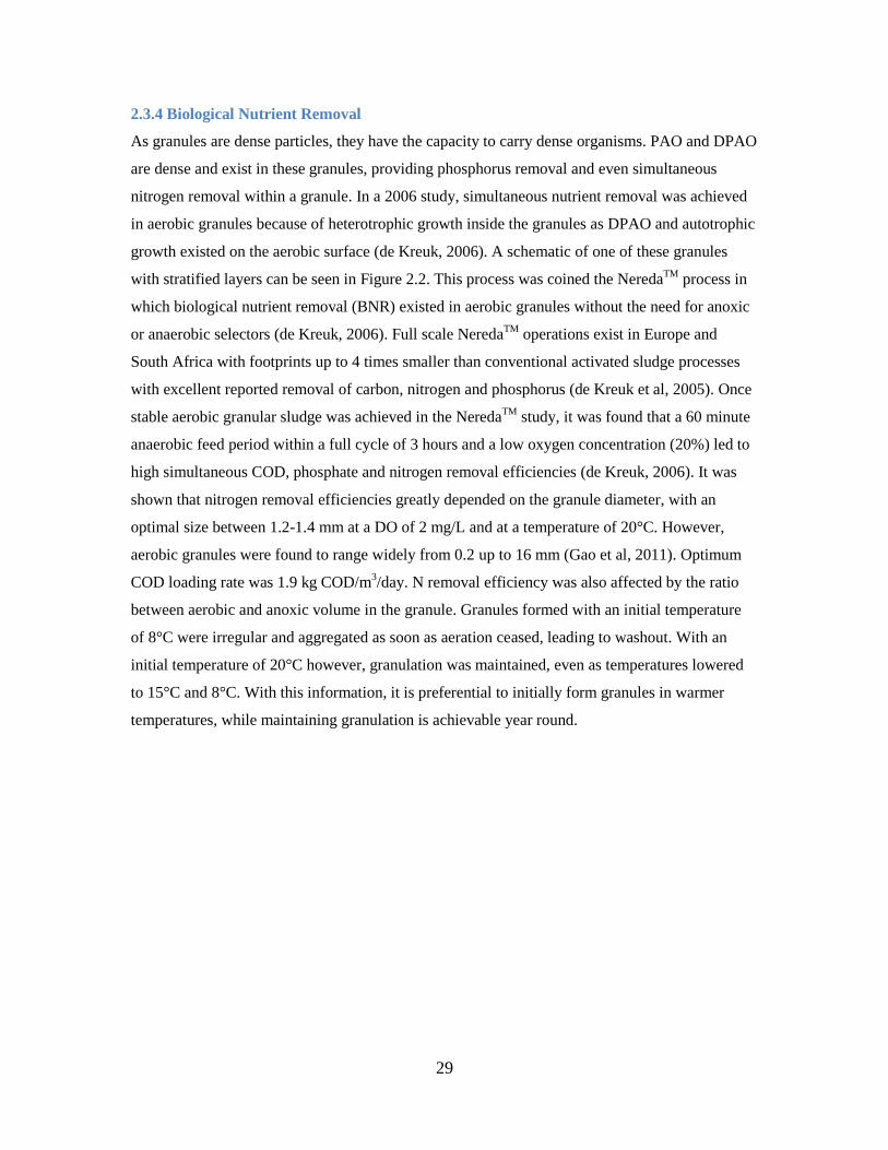
29
2.3.4 Biological Nutrient Removal
As granules are dense particles, they have the capacity to carry dense organisms. PAO and DPAO
are dense and exist in these granules, providing phosphorus removal and even simultaneous
nitrogen removal within a granule. In a 2006 study, simultaneous nutrient removal was achieved
in aerobic granules because of heterotrophic growth inside the granules as DPAO and autotrophic
growth existed on the aerobic surface (de Kreuk, 2006). A schematic of one of these granules
with stratified layers can be seen in Figure 2.2. This process was coined the NeredaTM
process in
which biological nutrient removal (BNR) existed in aerobic granules without the need for anoxic
or anaerobic selectors (de Kreuk, 2006). Full scale NeredaTM
operations exist in Europe and
South Africa with footprints up to 4 times smaller than conventional activated sludge processes
with excellent reported removal of carbon, nitrogen and phosphorus (de Kreuk et al, 2005). Once
stable aerobic granular sludge was achieved in the NeredaTM
study, it was found that a 60 minute
anaerobic feed period within a full cycle of 3 hours and a low oxygen concentration (20%) led to
high simultaneous COD, phosphate and nitrogen removal efficiencies (de Kreuk, 2006). It was
shown that nitrogen removal efficiencies greatly depended on the granule diameter, with an
optimal size between 1.2-1.4 mm at a DO of 2 mg/L and at a temperature of 20°C. However,
aerobic granules were found to range widely from 0.2 up to 16 mm (Gao et al, 2011). Optimum
COD loading rate was 1.9 kg COD/m3/day. N removal efficiency was also affected by the ratio
between aerobic and anoxic volume in the granule. Granules formed with an initial temperature
of 8°C were irregular and aggregated as soon as aeration ceased, leading to washout. With an
initial temperature of 20°C however, granulation was maintained, even as temperatures lowered
to 15°C and 8°C. With this information, it is preferential to initially form granules in warmer
temperatures, while maintaining granulation is achievable year round.
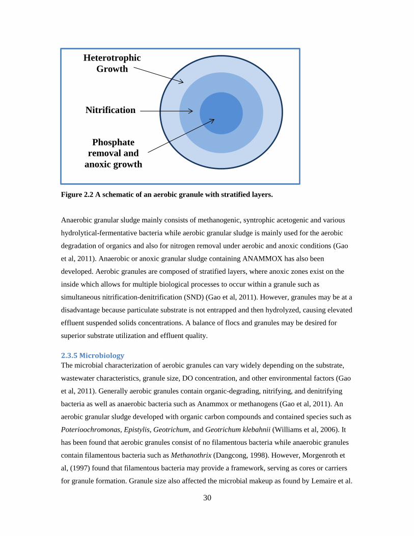
30
Figure 2.2 A schematic of an aerobic granule with stratified layers.
Anaerobic granular sludge mainly consists of methanogenic, syntrophic acetogenic and various
hydrolytical-fermentative bacteria while aerobic granular sludge is mainly used for the aerobic
degradation of organics and also for nitrogen removal under aerobic and anoxic conditions (Gao
et al, 2011). Anaerobic or anoxic granular sludge containing ANAMMOX has also been
developed. Aerobic granules are composed of stratified layers, where anoxic zones exist on the
inside which allows for multiple biological processes to occur within a granule such as
simultaneous nitrification-denitrification (SND) (Gao et al, 2011). However, granules may be at a
disadvantage because particulate substrate is not entrapped and then hydrolyzed, causing elevated
effluent suspended solids concentrations. A balance of flocs and granules may be desired for
superior substrate utilization and effluent quality.
2.3.5 Microbiology
The microbial characterization of aerobic granules can vary widely depending on the substrate,
wastewater characteristics, granule size, DO concentration, and other environmental factors (Gao
et al, 2011). Generally aerobic granules contain organic-degrading, nitrifying, and denitrifying
bacteria as well as anaerobic bacteria such as Anammox or methanogens (Gao et al, 2011). An
aerobic granular sludge developed with organic carbon compounds and contained species such as
Poterioochromonas, Epistylis, Geotrichum, and Geotrichum klebahnii (Williams et al, 2006). It
has been found that aerobic granules consist of no filamentous bacteria while anaerobic granules
contain filamentous bacteria such as Methanothrix (Dangcong, 1998). However, Morgenroth et
al, (1997) found that filamentous bacteria may provide a framework, serving as cores or carriers
for granule formation. Granule size also affected the microbial makeup as found by Lemaire et al.
Heterotrophic
Growth
Phosphate
removal and
anoxic growth
Nitrification
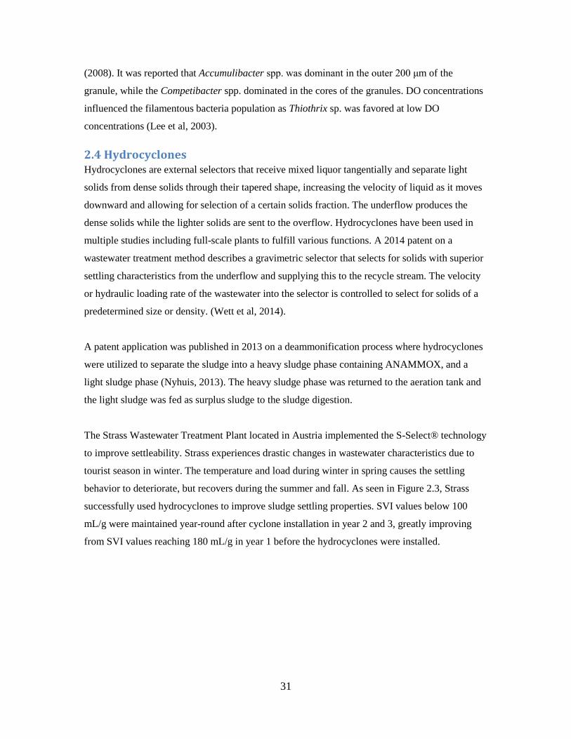
31
(2008). It was reported that Accumulibacter spp. was dominant in the outer 200 μm of the
granule, while the Competibacter spp. dominated in the cores of the granules. DO concentrations
influenced the filamentous bacteria population as Thiothrix sp. was favored at low DO
concentrations (Lee et al, 2003).
2.4 Hydrocyclones Hydrocyclones are external selectors that receive mixed liquor tangentially and separate light
solids from dense solids through their tapered shape, increasing the velocity of liquid as it moves
downward and allowing for selection of a certain solids fraction. The underflow produces the
dense solids while the lighter solids are sent to the overflow. Hydrocyclones have been used in
multiple studies including full-scale plants to fulfill various functions. A 2014 patent on a
wastewater treatment method describes a gravimetric selector that selects for solids with superior
settling characteristics from the underflow and supplying this to the recycle stream. The velocity
or hydraulic loading rate of the wastewater into the selector is controlled to select for solids of a
predetermined size or density. (Wett et al, 2014).
A patent application was published in 2013 on a deammonification process where hydrocyclones
were utilized to separate the sludge into a heavy sludge phase containing ANAMMOX, and a
light sludge phase (Nyhuis, 2013). The heavy sludge phase was returned to the aeration tank and
the light sludge was fed as surplus sludge to the sludge digestion.
The Strass Wastewater Treatment Plant located in Austria implemented the S-Select® technology
to improve settleability. Strass experiences drastic changes in wastewater characteristics due to
tourist season in winter. The temperature and load during winter in spring causes the settling
behavior to deteriorate, but recovers during the summer and fall. As seen in Figure 2.3, Strass
successfully used hydrocyclones to improve sludge settling properties. SVI values below 100
mL/g were maintained year-round after cyclone installation in year 2 and 3, greatly improving
from SVI values reaching 180 mL/g in year 1 before the hydrocyclones were installed.
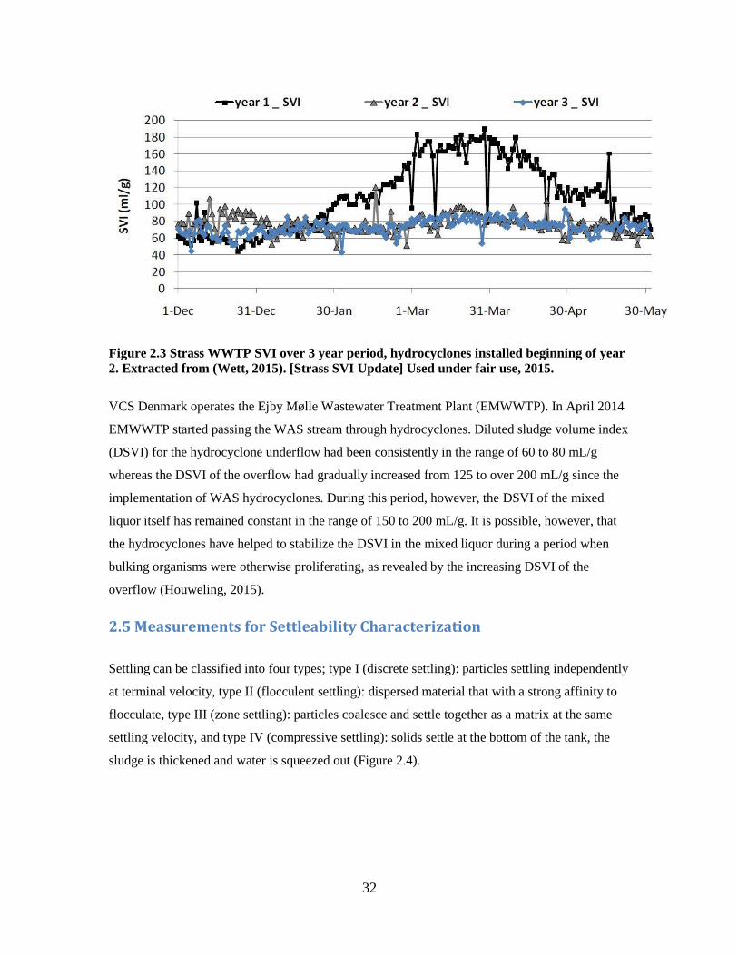
32
Figure 2.3 Strass WWTP SVI over 3 year period, hydrocyclones installed beginning of year
2. Extracted from (Wett, 2015). [Strass SVI Update] Used under fair use, 2015.
VCS Denmark operates the Ejby Mølle Wastewater Treatment Plant (EMWWTP). In April 2014
EMWWTP started passing the WAS stream through hydrocyclones. Diluted sludge volume index
(DSVI) for the hydrocyclone underflow had been consistently in the range of 60 to 80 mL/g
whereas the DSVI of the overflow had gradually increased from 125 to over 200 mL/g since the
implementation of WAS hydrocyclones. During this period, however, the DSVI of the mixed
liquor itself has remained constant in the range of 150 to 200 mL/g. It is possible, however, that
the hydrocyclones have helped to stabilize the DSVI in the mixed liquor during a period when
bulking organisms were otherwise proliferating, as revealed by the increasing DSVI of the
overflow (Houweling, 2015).
2.5 Measurements for Settleability Characterization
Settling can be classified into four types; type I (discrete settling): particles settling independently
at terminal velocity, type II (flocculent settling): dispersed material that with a strong affinity to
flocculate, type III (zone settling): particles coalesce and settle together as a matrix at the same
settling velocity, and type IV (compressive settling): solids settle at the bottom of the tank, the
sludge is thickened and water is squeezed out (Figure 2.4).
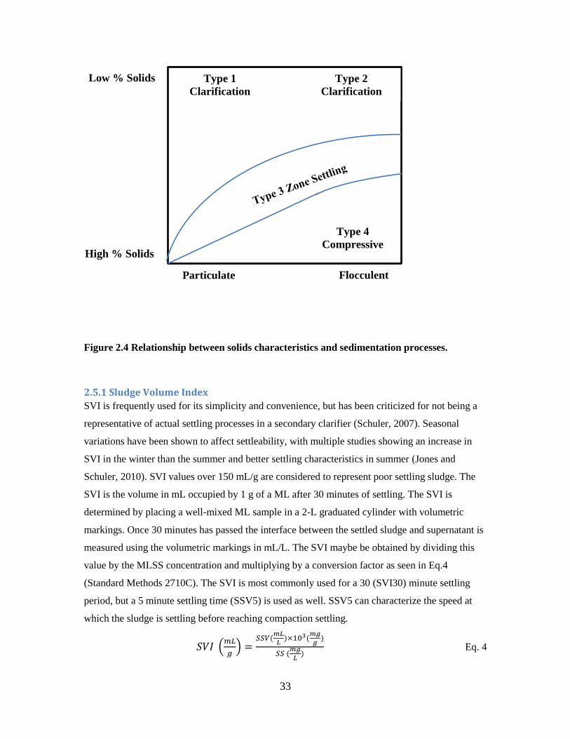
33
Figure 2.4 Relationship between solids characteristics and sedimentation processes.
2.5.1 Sludge Volume Index
SVI is frequently used for its simplicity and convenience, but has been criticized for not being a
representative of actual settling processes in a secondary clarifier (Schuler, 2007). Seasonal
variations have been shown to affect settleability, with multiple studies showing an increase in
SVI in the winter than the summer and better settling characteristics in summer (Jones and
Schuler, 2010). SVI values over 150 mL/g are considered to represent poor settling sludge. The
SVI is the volume in mL occupied by 1 g of a ML after 30 minutes of settling. The SVI is
determined by placing a well-mixed ML sample in a 2-L graduated cylinder with volumetric
markings. Once 30 minutes has passed the interface between the settled sludge and supernatant is
measured using the volumetric markings in mL/L. The SVI maybe be obtained by dividing this
value by the MLSS concentration and multiplying by a conversion factor as seen in Eq.4
(Standard Methods 2710C). The SVI is most commonly used for a 30 (SVI30) minute settling
period, but a 5 minute settling time (SSV5) is used as well. SSV5 can characterize the speed at
which the sludge is settling before reaching compaction settling.
(
)
Eq. 4
Type 1
Clarification
Type 4
Compressive High % Solids
Flocculent
Low % Solids Type 2
Clarification
Particulate
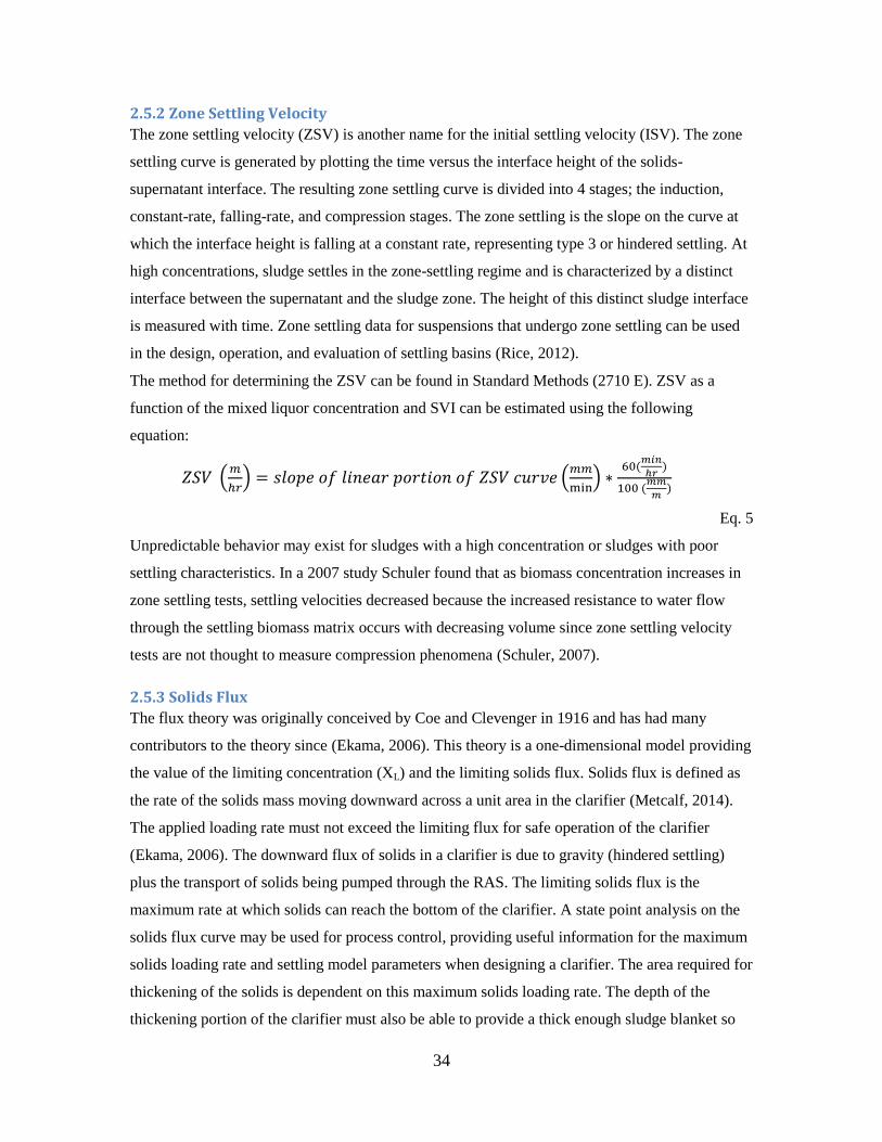
34
2.5.2 Zone Settling Velocity
The zone settling velocity (ZSV) is another name for the initial settling velocity (ISV). The zone
settling curve is generated by plotting the time versus the interface height of the solids-
supernatant interface. The resulting zone settling curve is divided into 4 stages; the induction,
constant-rate, falling-rate, and compression stages. The zone settling is the slope on the curve at
which the interface height is falling at a constant rate, representing type 3 or hindered settling. At
high concentrations, sludge settles in the zone-settling regime and is characterized by a distinct
interface between the supernatant and the sludge zone. The height of this distinct sludge interface
is measured with time. Zone settling data for suspensions that undergo zone settling can be used
in the design, operation, and evaluation of settling basins (Rice, 2012).
The method for determining the ZSV can be found in Standard Methods (2710 E). ZSV as a
function of the mixed liquor concentration and SVI can be estimated using the following
equation:
(
) (
)
Eq. 5
Unpredictable behavior may exist for sludges with a high concentration or sludges with poor
settling characteristics. In a 2007 study Schuler found that as biomass concentration increases in
zone settling tests, settling velocities decreased because the increased resistance to water flow
through the settling biomass matrix occurs with decreasing volume since zone settling velocity
tests are not thought to measure compression phenomena (Schuler, 2007).
2.5.3 Solids Flux
The flux theory was originally conceived by Coe and Clevenger in 1916 and has had many
contributors to the theory since (Ekama, 2006). This theory is a one-dimensional model providing
the value of the limiting concentration (XL) and the limiting solids flux. Solids flux is defined as
the rate of the solids mass moving downward across a unit area in the clarifier (Metcalf, 2014).
The applied loading rate must not exceed the limiting flux for safe operation of the clarifier
(Ekama, 2006). The downward flux of solids in a clarifier is due to gravity (hindered settling)
plus the transport of solids being pumped through the RAS. The limiting solids flux is the
maximum rate at which solids can reach the bottom of the clarifier. A state point analysis on the
solids flux curve may be used for process control, providing useful information for the maximum
solids loading rate and settling model parameters when designing a clarifier. The area required for
thickening of the solids is dependent on this maximum solids loading rate. The depth of the
thickening portion of the clarifier must also be able to provide a thick enough sludge blanket so
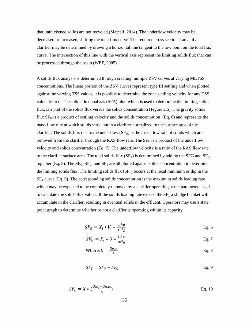
35
that unthickened solids are not recycled (Metcalf, 2014). The underflow velocity may be
decreased or increased, shifting the total flux curve. The required cross sectional area of a
clarifier may be determined by drawing a horizontal line tangent to the low point on the total flux
curve. The intersection of this line with the vertical axis represent the limiting solids flux that can
be processed through the basin (WEF, 2005).
A solids flux analysis is determined through creating multiple ZSV curves at varying MLTSS
concentrations. The linear portion of the ZSV curves represent type III settling and when plotted
against the varying TSS values, it is possible to determine the zone settling velocity for any TSS
value desired. The solids flux analysis (SFA) plot, which is used to determine the limiting solids
flux, is a plot of the solids flux versus the solids concentration (Figure 2.5). The gravity solids
flux SFG is a product of settling velocity and the solids concentration (Eq. 6) and represents the
mass flow rate at which solids settle out in a clarifier normalized to the surface area of the
clarifier. The solids flux due to the underflow (SFU) is the mass flow rate of solids which are
removed from the clarifier through the RAS flow rate. The SFU is a product of the underflow
velocity and solids concentration (Eq. 7). The underflow velocity is a ratio of the RAS flow rate
to the clarifier surface area. The total solids flux (SFT) is determined by adding the SFG and SFU
together (Eq. 8). The SFG, SFU, and SFT are all plotted against solids concentration to determine
the limiting solids flux. The limiting solids flux (SFL) occurs at the local minimum or dip in the
SFT curve (Eq. 9). The corresponding solids concentration is the maximum solids loading rate
which may be expected to be completely removed by a clarifier operating at the parameters used
to calculate the solids flux values. If the solids loading rate exceed the SFL a sludge blanket will
accumulate in the clarifier, resulting in eventual solids in the effluent. Operators may use a state
point graph to determine whether or not a clarifier is operating within its capacity.
Eq. 6
Eq. 7
Eq. 8
Eq. 9
Eq. 10
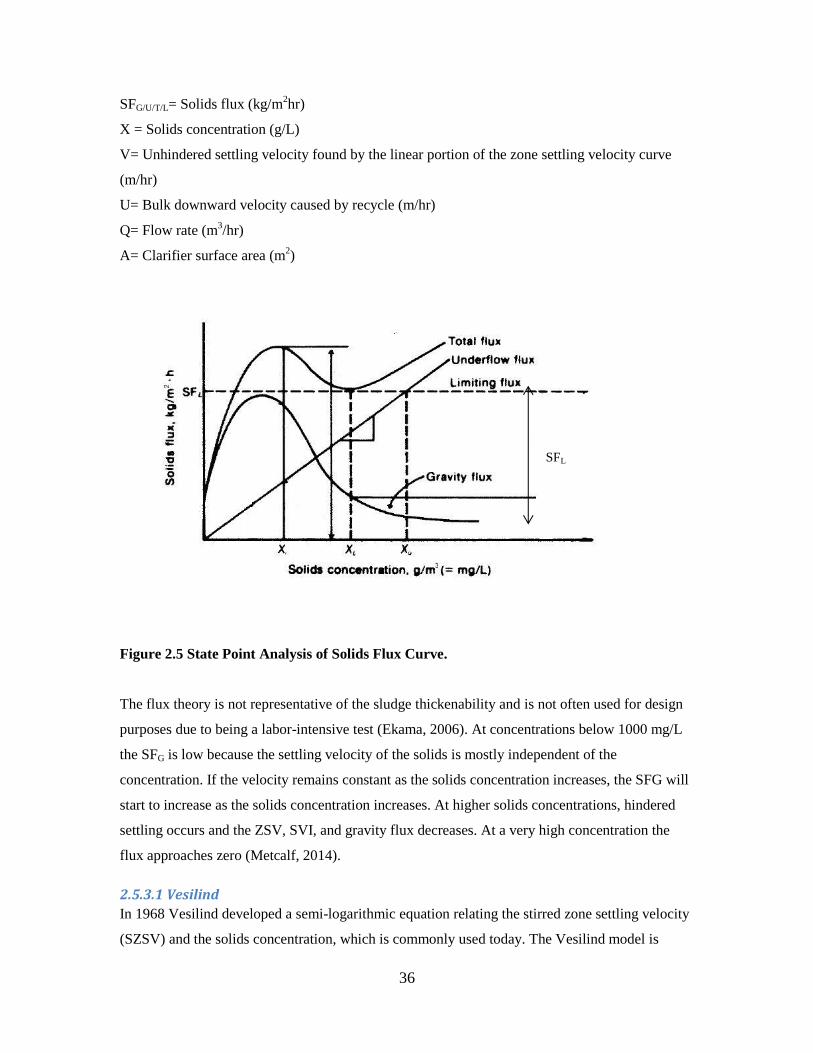
36
SFG/U/T/L= Solids flux (kg/m2hr)
X = Solids concentration (g/L)
V= Unhindered settling velocity found by the linear portion of the zone settling velocity curve
(m/hr)
U= Bulk downward velocity caused by recycle (m/hr)
Q= Flow rate (m3/hr)
A= Clarifier surface area (m2)
Figure 2.5 State Point Analysis of Solids Flux Curve.
The flux theory is not representative of the sludge thickenability and is not often used for design
purposes due to being a labor-intensive test (Ekama, 2006). At concentrations below 1000 mg/L
the SFG is low because the settling velocity of the solids is mostly independent of the
concentration. If the velocity remains constant as the solids concentration increases, the SFG will
start to increase as the solids concentration increases. At higher solids concentrations, hindered
settling occurs and the ZSV, SVI, and gravity flux decreases. At a very high concentration the
flux approaches zero (Metcalf, 2014).
2.5.3.1 Vesilind
In 1968 Vesilind developed a semi-logarithmic equation relating the stirred zone settling velocity
(SZSV) and the solids concentration, which is commonly used today. The Vesilind model is
SFL
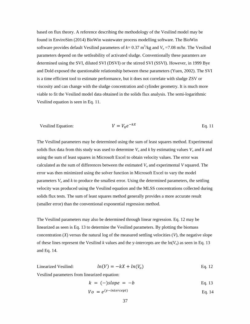
37
based on flux theory. A reference describing the methodology of the Vesilind model may be
found in EnviroSim (2014) BioWin wastewater process modelling software. The BioWin
software provides default Vesilind parameters of k= 0.37 m3/kg and Vo =7.08 m/hr. The Vesilind
parameters depend on the settleability of activated sludge. Conventionally these paramters are
determined using the SVI, diluted SVI (DSVI) or the stirred SVI (SSVI). However, in 1999 Bye
and Dold exposed the questionable relationship between these parameters (Yuen, 2002). The SVI
is a time efficient tool to estimate performance, but it does not correlate with sludge ZSV or
viscosity and can change with the sludge concentration and cylinder geometry. It is much more
viable to fit the Vesilind model data obtained in the solids flux analysis. The semi-logarithmic
Vesilind equation is seen in Eq. 11.
Vesilind Equation: Eq. 11
The Vesilind parameters may be determined using the sum of least squares method. Experimental
solids flux data from this study was used to determine Vo and k by estimating values Vo and k and
using the sum of least squares in Microsoft Excel to obtain velocity values. The error was
calculated as the sum of differences between the estimated Vo and experimental V squared. The
error was then minimized using the solver function in Microsoft Excel to vary the model
parameters Vo and k to produce the smallest error. Using the determined parameters, the settling
velocity was produced using the Vesilind equation and the MLSS concentrations collected during
solids flux tests. The sum of least squares method generally provides a more accurate result
(smaller error) than the conventional exponential regression method.
The Vesilind parameters may also be determined through linear regression. Eq. 12 may be
linearized as seen is Eq. 13 to determine the Vesilind parameters. By plotting the biomass
concentration (X) versus the natural log of the measured settling velocities (V), the negative slope
of these lines represent the Vesilind k values and the y-intercepts are the ln(Vo) as seen in Eq. 13
and Eq. 14.
Linearized Vesilind: Eq. 12
Vesilind parameters from linearized equation:
Eq. 13
Eq. 14

38
V= Settling velocity (m/s)
X= Biomass Density (g/L)
Vo= constant (m/s)
k= constant (m3/kg)
Well settling sludges may have max settling velocities (Vo) of around 13 m/hr versus 5 m/hr or
less for poor settling sludges. The Vesilind constant (k) is typically low for well settling sludges:
around 0.25 m3/kg is excellent and 0.5 m
3/kg is poor (Ekama, 2006). It has been suggested that
the coefficient Vo in the Vesilind equation form is related to Stokes-type settling for an individual
floc, while k may represent factors affecting compaction or factors that contribute to resistance of
settling (Schuler, 2007). Figure 2.6 represents a model of the semi-logarithmic Vesilind equation.
Region 1 represents the non-settleable solids, Region 2 represents the low solids concentration,
whereby discrete settling is in effect, Region 3 represents flocculent settling which is assumed to
be independent of solids concentration and is a function of the maximum settling velocity, and
Region 4 is the non stokian region that described hindered and compressional settling (Mancell-
Egala, In Preparation). The highest settling occurs during flocculent settling and as it transitions
into non-stokian settling, velocity decreases.
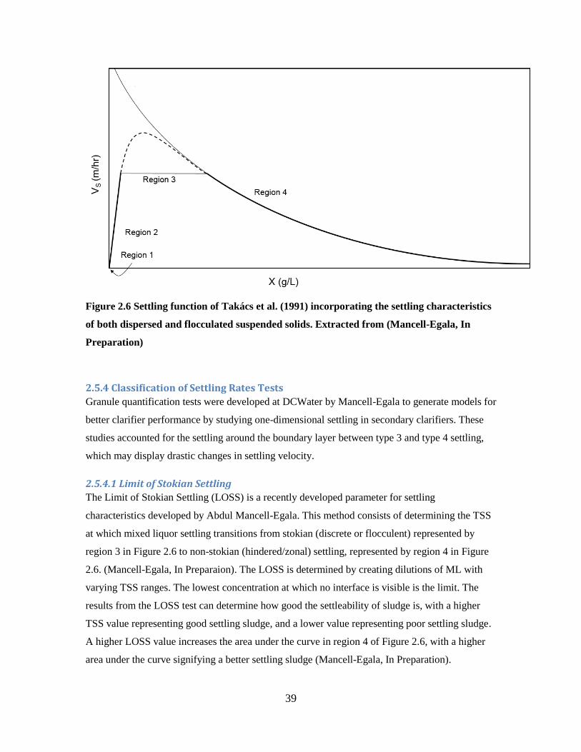
39
Figure 2.6 Settling function of Takács et al. (1991) incorporating the settling characteristics
of both dispersed and flocculated suspended solids. Extracted from (Mancell-Egala, In
Preparation)
2.5.4 Classification of Settling Rates Tests
Granule quantification tests were developed at DCWater by Mancell-Egala to generate models for
better clarifier performance by studying one-dimensional settling in secondary clarifiers. These
studies accounted for the settling around the boundary layer between type 3 and type 4 settling,
which may display drastic changes in settling velocity.
2.5.4.1 Limit of Stokian Settling
The Limit of Stokian Settling (LOSS) is a recently developed parameter for settling
characteristics developed by Abdul Mancell-Egala. This method consists of determining the TSS
at which mixed liquor settling transitions from stokian (discrete or flocculent) represented by
region 3 in Figure 2.6 to non-stokian (hindered/zonal) settling, represented by region 4 in Figure
2.6. (Mancell-Egala, In Preparaion). The LOSS is determined by creating dilutions of ML with
varying TSS ranges. The lowest concentration at which no interface is visible is the limit. The
results from the LOSS test can determine how good the settleability of sludge is, with a higher
TSS value representing good settling sludge, and a lower value representing poor settling sludge.
A higher LOSS value increases the area under the curve in region 4 of Figure 2.6, with a higher
area under the curve signifying a better settling sludge (Mancell-Egala, In Preparation).
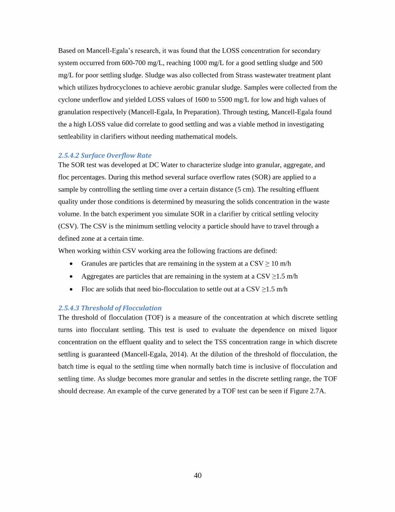
40
Based on Mancell-Egala’s research, it was found that the LOSS concentration for secondary
system occurred from 600-700 mg/L, reaching 1000 mg/L for a good settling sludge and 500
mg/L for poor settling sludge. Sludge was also collected from Strass wastewater treatment plant
which utilizes hydrocyclones to achieve aerobic granular sludge. Samples were collected from the
cyclone underflow and yielded LOSS values of 1600 to 5500 mg/L for low and high values of
granulation respectively (Mancell-Egala, In Preparation). Through testing, Mancell-Egala found
the a high LOSS value did correlate to good settling and was a viable method in investigating
settleability in clarifiers without needing mathematical models.
2.5.4.2 Surface Overflow Rate
The SOR test was developed at DC Water to characterize sludge into granular, aggregate, and
floc percentages. During this method several surface overflow rates (SOR) are applied to a
sample by controlling the settling time over a certain distance (5 cm). The resulting effluent
quality under those conditions is determined by measuring the solids concentration in the waste
volume. In the batch experiment you simulate SOR in a clarifier by critical settling velocity
(CSV). The CSV is the minimum settling velocity a particle should have to travel through a
defined zone at a certain time.
When working within CSV working area the following fractions are defined:
Granules are particles that are remaining in the system at a CSV ≥ 10 m/h
Aggregates are particles that are remaining in the system at a CSV ≥1.5 m/h
Floc are solids that need bio-flocculation to settle out at a CSV ≥1.5 m/h
2.5.4.3 Threshold of Flocculation
The threshold of flocculation (TOF) is a measure of the concentration at which discrete settling
turns into flocculant settling. This test is used to evaluate the dependence on mixed liquor
concentration on the effluent quality and to select the TSS concentration range in which discrete
settling is guaranteed (Mancell-Egala, 2014). At the dilution of the threshold of flocculation, the
batch time is equal to the settling time when normally batch time is inclusive of flocculation and
settling time. As sludge becomes more granular and settles in the discrete settling range, the TOF
should decrease. An example of the curve generated by a TOF test can be seen if Figure 2.7A.
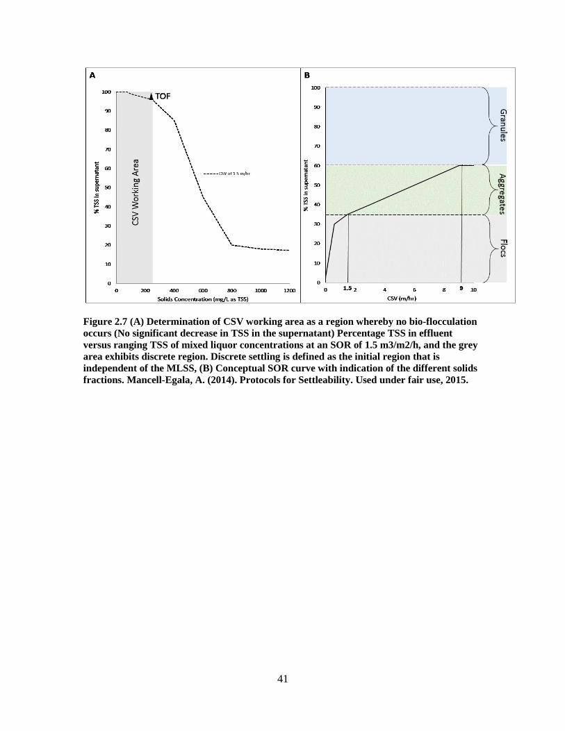
41
Figure 2.7 (A) Determination of CSV working area as a region whereby no bio-flocculation
occurs (No significant decrease in TSS in the supernatant) Percentage TSS in effluent
versus ranging TSS of mixed liquor concentrations at an SOR of 1.5 m3/m2/h, and the grey
area exhibits discrete region. Discrete settling is defined as the initial region that is
independent of the MLSS, (B) Conceptual SOR curve with indication of the different solids
fractions. Mancell-Egala, A. (2014). Protocols for Settleability. Used under fair use, 2015.
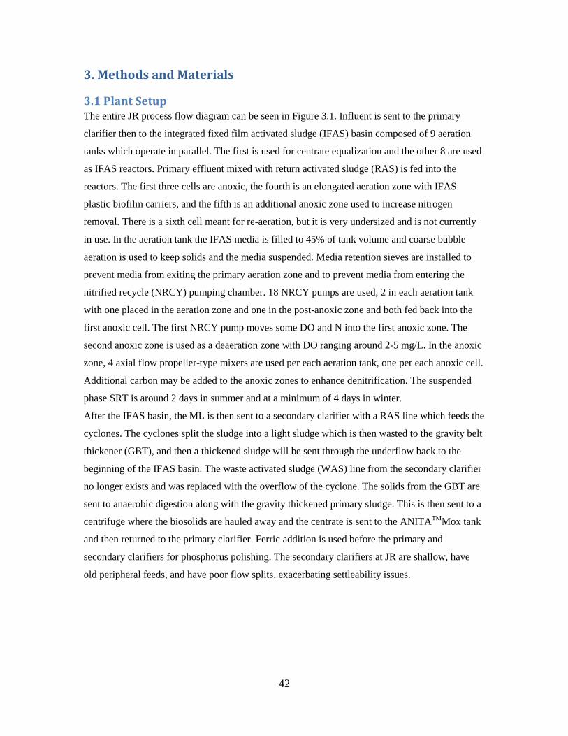
42
3. Methods and Materials
3.1 Plant Setup The entire JR process flow diagram can be seen in Figure 3.1. Influent is sent to the primary
clarifier then to the integrated fixed film activated sludge (IFAS) basin composed of 9 aeration
tanks which operate in parallel. The first is used for centrate equalization and the other 8 are used
as IFAS reactors. Primary effluent mixed with return activated sludge (RAS) is fed into the
reactors. The first three cells are anoxic, the fourth is an elongated aeration zone with IFAS
plastic biofilm carriers, and the fifth is an additional anoxic zone used to increase nitrogen
removal. There is a sixth cell meant for re-aeration, but it is very undersized and is not currently
in use. In the aeration tank the IFAS media is filled to 45% of tank volume and coarse bubble
aeration is used to keep solids and the media suspended. Media retention sieves are installed to
prevent media from exiting the primary aeration zone and to prevent media from entering the
nitrified recycle (NRCY) pumping chamber. 18 NRCY pumps are used, 2 in each aeration tank
with one placed in the aeration zone and one in the post-anoxic zone and both fed back into the
first anoxic cell. The first NRCY pump moves some DO and N into the first anoxic zone. The
second anoxic zone is used as a deaeration zone with DO ranging around 2-5 mg/L. In the anoxic
zone, 4 axial flow propeller-type mixers are used per each aeration tank, one per each anoxic cell.
Additional carbon may be added to the anoxic zones to enhance denitrification. The suspended
phase SRT is around 2 days in summer and at a minimum of 4 days in winter.
After the IFAS basin, the ML is then sent to a secondary clarifier with a RAS line which feeds the
cyclones. The cyclones split the sludge into a light sludge which is then wasted to the gravity belt
thickener (GBT), and then a thickened sludge will be sent through the underflow back to the
beginning of the IFAS basin. The waste activated sludge (WAS) line from the secondary clarifier
no longer exists and was replaced with the overflow of the cyclone. The solids from the GBT are
sent to anaerobic digestion along with the gravity thickened primary sludge. This is then sent to a
centrifuge where the biosolids are hauled away and the centrate is sent to the ANITATM
Mox tank
and then returned to the primary clarifier. Ferric addition is used before the primary and
secondary clarifiers for phosphorus polishing. The secondary clarifiers at JR are shallow, have
old peripheral feeds, and have poor flow splits, exacerbating settleability issues.
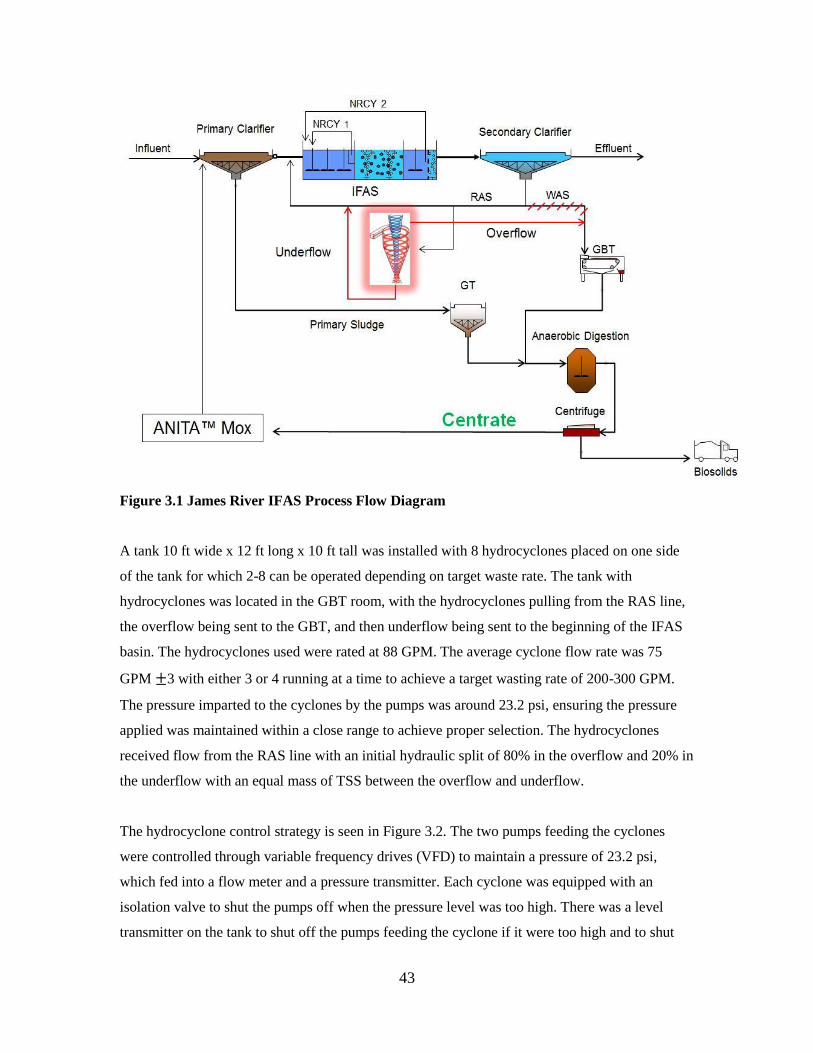
43
Figure 3.1 James River IFAS Process Flow Diagram
A tank 10 ft wide x 12 ft long x 10 ft tall was installed with 8 hydrocyclones placed on one side
of the tank for which 2-8 can be operated depending on target waste rate. The tank with
hydrocyclones was located in the GBT room, with the hydrocyclones pulling from the RAS line,
the overflow being sent to the GBT, and then underflow being sent to the beginning of the IFAS
basin. The hydrocyclones used were rated at 88 GPM. The average cyclone flow rate was 75
GPM 3 with either 3 or 4 running at a time to achieve a target wasting rate of 200-300 GPM.
The pressure imparted to the cyclones by the pumps was around 23.2 psi, ensuring the pressure
applied was maintained within a close range to achieve proper selection. The hydrocyclones
received flow from the RAS line with an initial hydraulic split of 80% in the overflow and 20% in
the underflow with an equal mass of TSS between the overflow and underflow.
The hydrocyclone control strategy is seen in Figure 3.2. The two pumps feeding the cyclones
were controlled through variable frequency drives (VFD) to maintain a pressure of 23.2 psi,
which fed into a flow meter and a pressure transmitter. Each cyclone was equipped with an
isolation valve to shut the pumps off when the pressure level was too high. There was a level
transmitter on the tank to shut off the pumps feeding the cyclone if it were too high and to shut
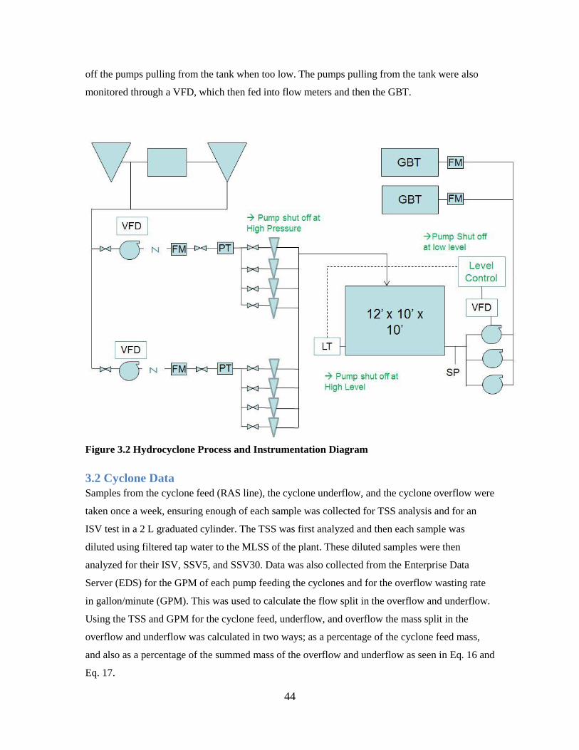
44
off the pumps pulling from the tank when too low. The pumps pulling from the tank were also
monitored through a VFD, which then fed into flow meters and then the GBT.
Figure 3.2 Hydrocyclone Process and Instrumentation Diagram
3.2 Cyclone Data
Samples from the cyclone feed (RAS line), the cyclone underflow, and the cyclone overflow were
taken once a week, ensuring enough of each sample was collected for TSS analysis and for an
ISV test in a 2 L graduated cylinder. The TSS was first analyzed and then each sample was
diluted using filtered tap water to the MLSS of the plant. These diluted samples were then
analyzed for their ISV, SSV5, and SSV30. Data was also collected from the Enterprise Data
Server (EDS) for the GPM of each pump feeding the cyclones and for the overflow wasting rate
in gallon/minute (GPM). This was used to calculate the flow split in the overflow and underflow.
Using the TSS and GPM for the cyclone feed, underflow, and overflow the mass split in the
overflow and underflow was calculated in two ways; as a percentage of the cyclone feed mass,
and also as a percentage of the summed mass of the overflow and underflow as seen in Eq. 16 and
Eq. 17.
45
(
)
Eq. 15
Eq. 16
(
)
Eq. 17
For continuing data collection, fresh samples will be taken after TSS analysis to prevent
denitrification in samples sitting while TSS is being run, which takes 1-1.5 h. Also, SCE will be
used for dilution rather than filtered tap water.
3.3 Plant Data
Plant data was collected from the James River plant operating reports beginning January 2011
when the IFAS reactor was fully implemented. Data was collected 3 days per week for MLTSS,
RAS TSS, SRT, SVI5, SVI30, Fe dosage, influent TP, effluent OP, and effluent TP. Filament
data were provided according to the filament index (FI) scale (0: none, 1: few, 2: some, 3:
common, 4: very common, 5: abundant, 6: excessive).
3.4 Sludge Volume Index (SVI) The SVI can be used to monitor settling characteristics of activated sludge and may be used for
process control. SVI5 and SVI30 were performed according to 2710C Standard Methods.
(
)
(Rice, 2012) Eq.18
The SVI is determined by placing a well-mixed ML sample in a 2-L graduated cylinder with
volumetric markings. Once 30 minutes has passed, the interface between the settled sludge and
supernatant is measured using the volumetric markings in mL/L to obtain the settled sludge
volume (SSV). The SVI is calculated as seen in Eq. 18. SVI5 and SVI30 values were obtained for
the cyclone underflow, cyclone overflow, RAS, ML, ML dilutions, and ML concentrations. These
values were tracked over time and compared to other parameters to characterize improvements in
settleability.
46
3.5 Zone Settling Velocity Settling is done at multiple concentrations; the original ML sample, 3 concentrations diluted
below, and 3 concentrations above the MLSS concentration. Concentrated mixtures were
achieved by allowing ML to settle and removing supernatant, then adding additional mixed
liquor. When diluting the ML, secondary effluent was used to ensure similar ionic characteristics.
The MLTSS was analyzed for only one of these concentrations. This TSS value was used to
calculate the varying TSS concentrations of the dilutions and concentrations, as these were simply
ratios of the raw mixed liquor. The zone settling velocity was also determined for the cyclone
feed (RAS), underflow, and overflow, initially diluting the samples to 3000 mg/L to represent the
MLTSS concentration of JR wastewater. The cyclone sampling points were later diluted to 2000
mg/L starting April 22nd
, 2015 to better represent varying JR MLTSS values, and then on June
3rd
, 2015 were again adjusted to 2500 mg/L dilutions for the most accurate result. These cyclone
sampling point ISVs were plotted against ML ISV values to see how settling velocities were
improving over time in the ML.
A 2 L settling column was used with a calibrating tape to represent distance in mm, while the
column measurements are conventionally volumetric. The sludge sample was mixed thoroughly
and poured into the cylinder while simultaneously starting a timer. The height of the solid-liquid
interface was recorded for time intervals of 30 s to 1 min for 30 minutes to observe a constant
zone-settling velocity. Once the rate of settling decreases, data collection ceased. Plots were
generated with interface height in cm vs. time in minutes, drawing a linear line through the linear
portion of the curve where settling rate is highest, corresponding to type III, or hindered settling
velocity. The settling rate is recorded as the slope of this line in units of m/hr.
3.6 Solids Flux The solids flux was determined by creating multiple dilutions and concentrations of JR ML
ranging from 0.7-4 g TSS/L and creating ZSV curves. The dilutions were made using ML
collected from the aeration effluent and diluting with filtered tap water which was assumed to
have a TSS of 0 g/L. For each test, a ZSV curve was created for the original ML sample, 3
dilutions below the MLTSS value, and 3 concentrations above the ML value for a total of 7
curves.
47
3.7 Classification of Settling Rates
3.7.1 Limit of Stokian Settling (LOSS)
The limit of stokian settling (LOSS) must first be determined before the SOR test can be
performed. A large amount of mixed liquor was collected at a point just before entering the
secondary clarifier. The dilutions were produced between the ranges of 250 mg TSS/L and 1000
mg TSS/L with a maximum gap between dilutions of 100 mg TSS/L. These diluted
concentrations were filled to the 2 L mark in settleometers and left to settle for less than a minute.
The lowest concentration at which no interface was visible was the limit. To find the minimum
ratio in which the interface was no longer visible, more dilutions between the concentrations
where no interface was visible and where an interface was visible were made. After creating more
dilutions between these two values, a more accurate value for the LOSS was obtained. This limit
was given as a concentration in mg/L.
3.7.2 Threshold of Flocculation (TOF)
The threshold of flocculation (TOF) is a measure of the concentration at which discrete settling
turns into flocculant settling. This test was used to evaluate the dependence of mixed liquor
concentration on the effluent quality and to select the TSS concentration range in which discrete
settling is guaranteed (Mancell-Egala, 2014).
At least 25 L of mixed liquor was collected at a point just before entering the secondary clarifier,
ensuring it was maintained at a constant temperature. The concentration of this mixed liquor was
used as the highest concentration and was then diluted multiple times with tap water to create
multiple varying concentrations (~6-8) of mixed liquor, covering concentrations ranging from
200-800 mg/L. 5 L of each concentration was made; 4 L to be used for settling and the excess to
be analyzed for TSS. Each concentration was then be poured into a 4 L graduated cylinder to the
fill line, then poured through a funnel into a 4 L graduated cylinder with ports to provide mixing.
The funnel was pulled as soon as the liquid reached the 4 L fill line, and the timer was started
simultaneously. The dilution was left to settle for 2 minutes equating to a CSV of 1.5 m/hr. At the
2 minute mark the clamps were opened so that the supernatant may be decanted off the top
through the tubes. The supernatant collected was then analyzed for TSS. 10-20 mL of liquid was
filtered for TSS, and duplicates were run for every concentration. Once the TSS was collected for
all concentrations, a graph was generated with the solids concentration on the x-axis and the %
solids in supernatant (Eq. 19) on the y-axis.
48
(
⁄ ) Eq. 19
The point at which line becomes linear is the minimum value of the solids concentration at which
flocculation occurs, or the TOF (the line should be S-shaped). The TOF was used as the
concentration in the SOR test. The SOR test uses one concentration over a period of different
settling times. The TSS range for which the fraction in effluent is independent of the sludge
mixture (beginning of the curve) is also the highest concentration where this is the true TOF. The
latter range is the range of discrete settling and is the target TSS range for SOR tests
Using the ratio obtained from the LOSS test, dilutions should be made with one concentration
being much higher than the LOSS, one at LOSS value, and then multiple concentrations at ratios
lower than LOSS down to a TSS of 100 mg/L when determining the TOF.
3.7.3 Surface Overflow Rate (SOR)
To conduct the SOR test, a 4 L plastic graduated cylinder with ports 5 cm below the 4 L fill line
must be made for decanting supernatant out of the top portion of the cylinder once the mixed
liquor has settled. The ports are located on opposite sides of the cylinder 5 cm below the 4 L fill
line. Each port is composed of a bulkhead fitting in which plastic tubing is attached. To prevent
liquid from flowing through the tubing, tubing clamps are fitted as close to the bulkhead as
possible. The tubing on both sides of the cylinder should be long enough to reach a device used
for collecting the sample.
A 4L graduated cylinder with no ports is used for filling mixed liquor to the 4 L fill line. Before
measuring out 4 L of liquid in the graduated cylinder, the mixed liquor must be stirred to ensure
proper mixing. Once 4 L is measured, some settling may have occurred, so the liquid is poured
from the initial graduated cylinder into the graduated cylinder with the port via a funnel placed on
top to provide adequate mixing. The timer set for the predetermined settling time is started as
soon as the liquid is filled and funnel is simultaneously removed. After it has settled for the
predetermined amount of time, the clamps will be opened, allowing the supernatant to decant out
of the top 5 cm of the graduated cylinder. The supernatant is then analyzed for TSS.
49
The concentration obtained as the TOF is used for this test. A large batch of this concentration is
made using mixed liquor which is collected from a point just before the secondary clarifier and
diluting it with tap water. The batch is stirred, poured into a 4 L graduated cylinder, and then
funneled into a 4 L graduated cylinder with ports to provide mixing. The test is run for settling
time periods of 20 s, 1 min, 2 min, 3 min, and 5 min, and then the supernatant decanted. TSS is
then analyzed for the supernatant of each sample and for the original TOF mixture. A plot is then
generated with the surface overflow rate on the x-axis, and the % solids in supernatant (Eq. 20)
on the y-axis, creating a histogram of the flocs. This characterizes the % of the sludge that has
good, medium, or poor settling based on the surface overflow rate.
The surface overflow rate is calculated as the distance of settling over the time period, the
distance being 5 cm and the time periods ranging from 20 s to 5 min.
(
⁄ ) Eq. 20
3.8 Floc Density The floc density of the ML at JR was measured routinely as it was expected to increase as the
sludge became more granular. Methods for the test were adapted from the 1985 GE Healthcare
and Life Sciences manual on Cell Separation Media (GE Healthcare and Life Sciences, 1985).
The density of the floc was measured using Percoll isopycnic centrifugation, the particles were
separated based solely on differences in density, irrespective of size. A Stock Isotonic Solution
(SIP) was created using 1.5 M NaCl, Percoll, and distilled water. Percoll is a high density (1.13
g/mL) solution with silica particles and a low osmotic pressure. To create the SIP, the desired
osmolality was determined by measuring the osmolality of the ML at JR. The density of the SIP
could be adjusted by changing the amount of NaCl in the solution. Calculations for determining
the SIP can be seen in Appendix F. An SIP batch was composed of 47.15 mL Percoll, 15 mL 1.5
M NaCl, and 37.85 mL distilled water. Using a high speed centrifuge, 2 16 mL tubes, density
gradient beads, and the SIP, a density gradient was made within the tubes. One tube was to show
the density gradient of the beads, which composed of 6 different bead colors ranging from 1.025-
1.130 g/mL. These densities were expected to bracket the density of the ML floc. The beads
created a distinct line within the tube, representing increasing density moving downwards. The
other tube was used for showing the floc density of the ML.
50
The high-speed centrifuge was set to 22°C. Initially, the 16 mL tubes were both filled with 14 mL
of SIP. 2 µL of each bead type added to one tube. Both tubes were then centrifuged at 15,000 G
for 30 min. Banding was not clearly defined, and beads were disturbed easily as they were pulled
from the centrifuge. To increase clarity of the density gradients, the run time in the centrifuge was
increased. After 3 attempts with an initial centrifuge run of 1 hour, the band formed by the beads
within the tube was not as defined as would be desired, so the initial centrifuge run time was
increased to 1.5 hr. The 16 mL tubes were also filled to 14.5 mL and 15.5 mL of SIP to reduce
amount of air space in the tube, reducing the disturbance in the tube when being removed from
the centrifuge. The tube filled with 14.5 mL SIP allowed for 1 mL of ML to be added after the
density gradient was formed in the initial 1.5 hr centrifuge run. After the ML was added, the tubes
were centrifuged again at 400 G for 15 min. and then removed from the centrifuge to be photo
analyzed for band height and floc height within tube. The density of the floc was interpolated
based on the measurements in the two tubes. Results from this test are highly precise as the
solution increments are fairly narrow relative to the biomass densities.
3.9 Filament Quantification and Identification
Samples of ML collected from the aeration effluent were sent periodically to Paul Pitt of Hazen
and Sawyer for microscopic analysis.
3.10 PAO Activity Tests The biological phosphorus activity test is a bench-scale phosphate uptake and release test adapted
from the WERF 2010 study (Neethling, 2005). This test measures the anaerobic phosphorus
release rates, anaerobic COD uptake rate, anaerobic phosphorus release to COD uptake rate ratio,
and aerobic phosphorus uptake rates to evaluate biological phosphorus removal. ML used for this
test was collected from the aeration effluent and aerated for approximately 1 hour to remove
excess ammonium. The sample was then put into a 2 L settleometer which was placed into a
water bath set to the plants current temperature while being continuously mixed using stir bars
and stir plates. As soon as the sample was placed in the water bath, an initial sample was
collected to be analyzed for TSS and TVSS. The beaker was then covered to reduce aeration to 0
mg/L for 10 minutes to allow the sample to acclimate. Then 100 mg/L COD (10 mL NaAc per 2
L) was added to the beaker and it was stirred and mixed for 90 minutes. The preliminary
phosphorus uptake period then starts by aerating the samples and monitoring the pH and DO
levels. Once the DO reached 2 mg/L, an initial sample was collected to be filtered and analyzed
for NH4+, NO3-, and NO2- using HACH tubes to ensure all concentrations were <2 mg/L,
51
otherwise the test would provide inaccurate results. If all initial HACH tubes were <2 mg/L, 4
mL Potassium Phosphate (K2HPO4)- was added and then the sample was aerated for 2 hours,
recording pH and DO every 15 minutes. After 2 hours, a sample was taken and analyzed for OP,
NH4+, NO3-, NO2- and sCOD; pH and DO. The air was then turned off for the anaerobic
phosphorus release and COD uptake period. The beakers were covered and sparged with N2 gas
to bring DO to 0 mg/L. The pH range of 6.8-7.5 was controlled by sparging with CO2 when pH
levels were too high. As DO reached 0 mg/L the beakers were covered, the N2/CO2 gas was
turned off, and 100 mg/L COD (10 ml NaAc stock) was added to the beaker. Immediately a
sample was taken and analyzed for OP, NH4+, NO3-, NO2-, sCOD, pH and DO. This was
repeated every 3 minutes for 15 minutes, and then every 15 minutes for an hour. The beakers
covers were then removed and air turned back on for the aerobic phosphorus uptake period. As
soon as the DO reached 2 mg/L, a sample was taken every 15 minutes for an 1.15 hr and analyzed
for OP, NH4+, NO3-, NO2-, pH and DO. Hach tubes were read using a DR 2800™
Spectrophotometer.
As of August 5th 2015, DPAO activity measurements were taken. DPAO activity was measured
by altering the existing biological phosphorus activity test to include an anoxic phase in addition
to an aerobic uptake phase. During what would usually be the aerobic phase, the system was kept
unaerated and 20 mg/L of NO3-N was added. The duration of the test was performed similarly; a
sample was taken every 15 minutes for an 1.15 hr and analyzed for OP, NH4+, NO3-, NO2-, pH
and DO. ML was measured using the original biological phosphorus activity test with the
anaerobic and aerobic phases in addition to the altered DPAO activity test with anaerobic and
anoxic phases. The results from this test provided data showing how much biological activity was
due to PAO or DPAO, as normal PAO take up phosphorus during aerobic conditions and DPAO
take up phosphorus in anoxic conditions.
3.11 AOB and NOB Activity Tests In order to measure AOB and NOB activity rates a 2 L sample was collected from the cyclone
feed, underflow, and overflow. The sample was aerated for 30 minutes to oxidize any excess
COD in order to prevent heterotrophic competition for O2. The 2 L container was then spiked
with 20 mg/L NH4+-N (dissolved ammonium chloride solution) and 5 mg/L NO2
--N (dissolved
sodium nitrite solution). The mixture was sampled continuously for 1 hour at 15 minute intervals
using a 50 mL syringe. All collected samples were filtered through 0.45 µm nylon filters and
analyzed for NH4+-N, NO2
--N, and NO3
--N.
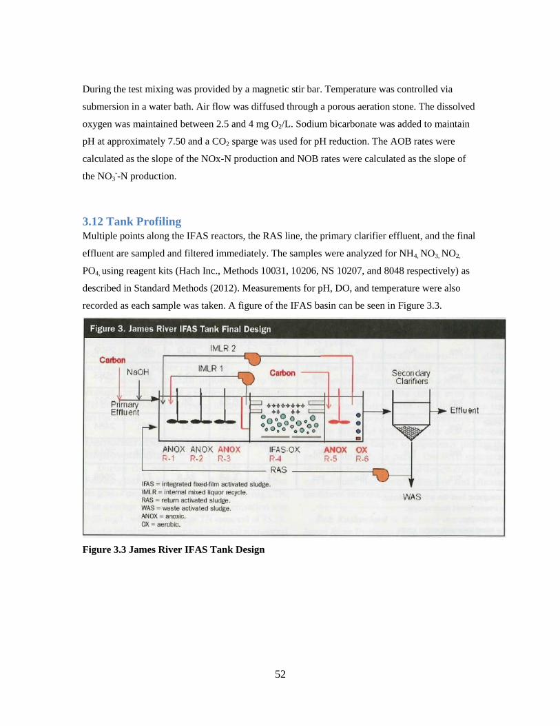
52
During the test mixing was provided by a magnetic stir bar. Temperature was controlled via
submersion in a water bath. Air flow was diffused through a porous aeration stone. The dissolved
oxygen was maintained between 2.5 and 4 mg O2/L. Sodium bicarbonate was added to maintain
pH at approximately 7.50 and a CO2 sparge was used for pH reduction. The AOB rates were
calculated as the slope of the NOx-N production and NOB rates were calculated as the slope of
the NO3--N production.
3.12 Tank Profiling
Multiple points along the IFAS reactors, the RAS line, the primary clarifier effluent, and the final
effluent are sampled and filtered immediately. The samples were analyzed for NH4, NO3, NO2,
PO4, using reagent kits (Hach Inc., Methods 10031, 10206, NS 10207, and 8048 respectively) as
described in Standard Methods (2012). Measurements for pH, DO, and temperature were also
recorded as each sample was taken. A figure of the IFAS basin can be seen in Figure 3.3.
Figure 3.3 James River IFAS Tank Design
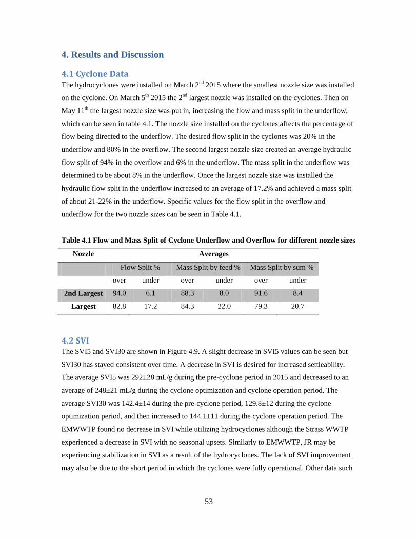
53
4. Results and Discussion
4.1 Cyclone Data The hydrocyclones were installed on March 2
nd 2015 where the smallest nozzle size was installed
on the cyclone. On March 5th 2015 the 2
nd largest nozzle was installed on the cyclones. Then on
May 11th the largest nozzle size was put in, increasing the flow and mass split in the underflow,
which can be seen in table 4.1. The nozzle size installed on the cyclones affects the percentage of
flow being directed to the underflow. The desired flow split in the cyclones was 20% in the
underflow and 80% in the overflow. The second largest nozzle size created an average hydraulic
flow split of 94% in the overflow and 6% in the underflow. The mass split in the underflow was
determined to be about 8% in the underflow. Once the largest nozzle size was installed the
hydraulic flow split in the underflow increased to an average of 17.2% and achieved a mass split
of about 21-22% in the underflow. Specific values for the flow split in the overflow and
underflow for the two nozzle sizes can be seen in Table 4.1.
Table 4.1 Flow and Mass Split of Cyclone Underflow and Overflow for different nozzle sizes
Nozzle Averages
Flow Split % Mass Split by feed % Mass Split by sum %
over under over under over under
2nd Largest 94.0 6.1 88.3 8.0 91.6 8.4
Largest 82.8 17.2 84.3 22.0 79.3 20.7
4.2 SVI
The SVI5 and SVI30 are shown in Figure 4.9. A slight decrease in SVI5 values can be seen but
SVI30 has stayed consistent over time. A decrease in SVI is desired for increased settleability.
The average SVI5 was 292±28 mL/g during the pre-cyclone period in 2015 and decreased to an
average of 248±21 mL/g during the cyclone optimization and cyclone operation period. The
average SVI30 was 142.4±14 during the pre-cyclone period, 129.8±12 during the cyclone
optimization period, and then increased to 144.1±11 during the cyclone operation period. The
EMWWTP found no decrease in SVI while utilizing hydrocyclones although the Strass WWTP
experienced a decrease in SVI with no seasonal upsets. Similarly to EMWWTP, JR may be
experiencing stabilization in SVI as a result of the hydrocyclones. The lack of SVI improvement
may also be due to the short period in which the cyclones were fully operational. Other data such
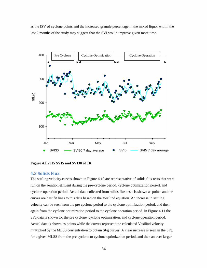
54
as the ISV of cyclone points and the increased granule percentage in the mixed liquor within the
last 2 months of the study may suggest that the SVI would improve given more time.
Jan Mar May Jul Sep
mL/g
100
200
300
400
SVI5SVI30 SVI5 7 day averageSVI30 7 day average
Figure 4.1 2015 SVI5 and SVI30 of JR
4.3 Solids Flux The settling velocity curves shown in Figure 4.10 are representative of solids flux tests that were
run on the aeration effluent during the pre-cyclone period, cyclone optimization period, and
cyclone operation period. Actual data collected from solids flux tests is shown as points and the
curves are best fit lines to this data based on the Vesilind equation. An increase in settling
velocity can be seen from the pre cyclone period to the cyclone optimization period, and then
again from the cyclone optimization period to the cyclone operation period. In Figure 4.11 the
SFg data is shown for the pre cyclone, cyclone optimization, and cyclone operation period.
Actual data is shown as points while the curves represent the calculated Vesilind velocity
multiplied by the MLSS concentration to obtain SFg curves. A clear increase is seen in the SFg
for a given MLSS from the pre cyclone to cyclone optimization period, and then an ever larger
Pre Cyclone Cyclone Optimization Cyclone Operation
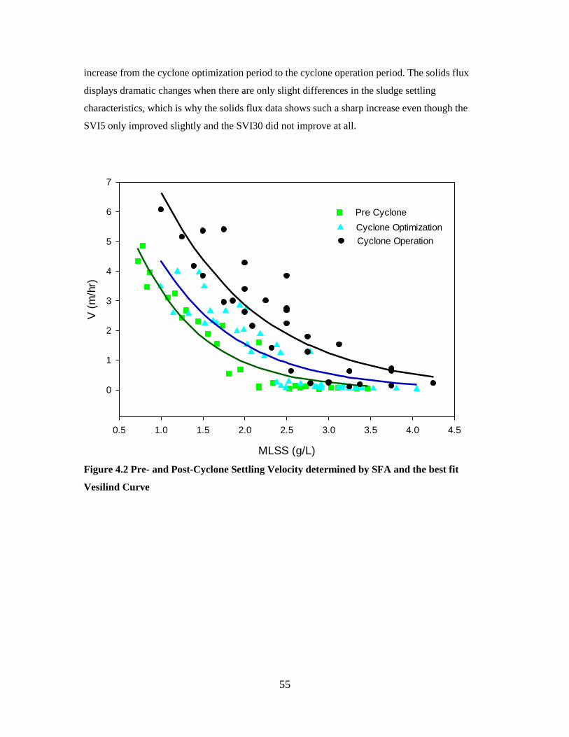
55
increase from the cyclone optimization period to the cyclone operation period. The solids flux
displays dramatic changes when there are only slight differences in the sludge settling
characteristics, which is why the solids flux data shows such a sharp increase even though the
SVI5 only improved slightly and the SVI30 did not improve at all.
MLSS (g/L)
0.5 1.0 1.5 2.0 2.5 3.0 3.5 4.0 4.5
V (
m/h
r)
0
1
2
3
4
5
6
7
Pre Cyclone
Cyclone Optimization
Cyclone Operation
Figure 4.2 Pre- and Post-Cyclone Settling Velocity determined by SFA and the best fit
Vesilind Curve
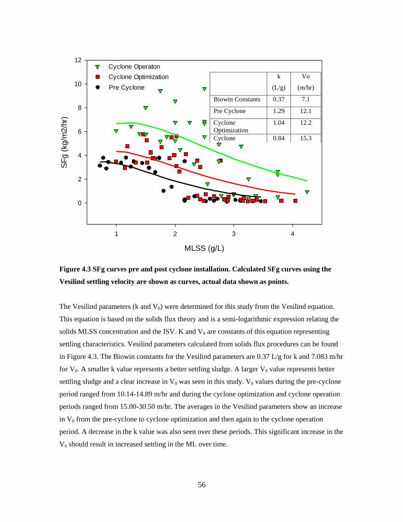
56
MLSS (g/L)
1 2 3 4
SF
g (
kg/m
2/h
r)
0
2
4
6
8
10
12
Pre Cyclone
Cyclone Optimization
Cyclone Operaton
Figure 4.3 SFg curves pre and post cyclone installation. Calculated SFg curves using the
Vesilind settling velocity are shown as curves, actual data shown as points.
The Vesilind parameters (k and V0) were determined for this study from the Vesilind equation.
This equation is based on the solids flux theory and is a semi-logarithmic expression relating the
solids MLSS concentration and the ISV. K and V0 are constants of this equation representing
settling characteristics. Vesilind parameters calculated from solids flux procedures can be found
in Figure 4.3. The Biowin constants for the Vesilind parameters are 0.37 L/g for k and 7.083 m/hr
for V0. A smaller k value represents a better settling sludge. A larger V0 value represents better
settling sludge and a clear increase in V0 was seen in this study. V0 values during the pre-cyclone
period ranged from 10.14-14.89 m/hr and during the cyclone optimization and cyclone operation
periods ranged from 15.00-30.50 m/hr. The averages in the Vesilind parameters show an increase
in V0 from the pre-cyclone to cyclone optimization and then again to the cyclone operation
period. A decrease in the k value was also seen over these periods. This significant increase in the
V0 should result in increased settling in the ML over time.
k
(L/g)
Vo
(m/hr)
Biowin Constants 0.37 7.1
Pre Cyclone 1.29 12.1
Cyclone
Optimization
1.04 12.2
Cyclone
Operation
0.84 15.3

57
4.4 Settleability
Figure 4.4 provides the ISV of the cyclone feed, underflow, and overflow all adjusted to 2500
mg/L. The data shown is only representative of the period when the cyclones were under full
operation. Cyclone overflow, underflow and feed and the aeration effluent were originally
adjusted to 3000 mg/L when calculating the ISV to compare all samples as this was close to the
MLSS concentration of James River. Beginning April 22, 2015, all samples were adjusted to
2000 mg/L as this better matched the MLSS concentration at the time. Then on June 3rd
2015 the
samples were all adjusted to 2500 mg/L, again because this better matched the MLSS
concentration.
Figure 4.4 does not show an increase in the ISV in the cyclone feed which is desired as it is
representative of the mixed liquor settling velocity. The important thing to note is the large
difference of the underflow and overflow settling velocity, showing the system selects for solids
settling at a higher rate. The cyclone feed had an average ISV of 1.5±1.1 m/hr, the cyclone
underflow had an average ISV of 2.5±1.3 m/hr and the cyclone overflow had an average ISV of
0.5±0.7 m/hr.
6.18
.15
7.8.
15
7.14
.15
7.16
.15
7.21
.15
7.27
.15
8.26
.15
9.7.
15
9.10
.15
ISV
(m
/hr)
0.0
1.0
2.0
3.0
4.0
5.0
Feed
Underflow
Overflow
Figure 4.4 ISV of Cyclone Points adjusted to 2500 mg/L
58
4.5 Classification of Settling Rates In Figure 4.5 the percentages of granules, aggregates, and flocs in the mixed liquor is presented
over time as determined by discrete settling. It is apparent that there is no granule percentage until
April 23rd
, 2015 during the cyclone optimization period where the percentage reached only 1.7%.
During the cyclone operation period percentages of granules reached high values of 23.5% and
40.4%. An increased granule percentage is desired for creating a balance of flocs and granules.
The aggregate percentage decreased over time while the floc percentage increased, although
neither followed an exact trend. However within the last three testing periods from August 26th,
2015 to September 19th 2015 the aggregate percentage ranged from 14.1-45.0% when it had
previously had an average of 84.8%. The aggregate percentage was the majority of the floc
characterization during pre-cyclone and cyclone optimization periods averaging 85.6±11% and
decreasing to 46.9±35%. The floc percentage within the last three testing periods increased to a
range of 41.5-62.3% when previously it had an average of 14.4%. The floc fraction showed a
large increase from the pre-cyclone and cyclone optimization to the cyclone operation period with
averages increasing from 13.9±11% to 36.9±22%. It is unclear why the aggregate percentage
decreased as the floc and granule percentages had such a high increase. The increase in granule
percentage is the important takeaway from these results and should result in an increase in
settling velocity and enhanced biological phosphorus removal as granules thrive within the
system.
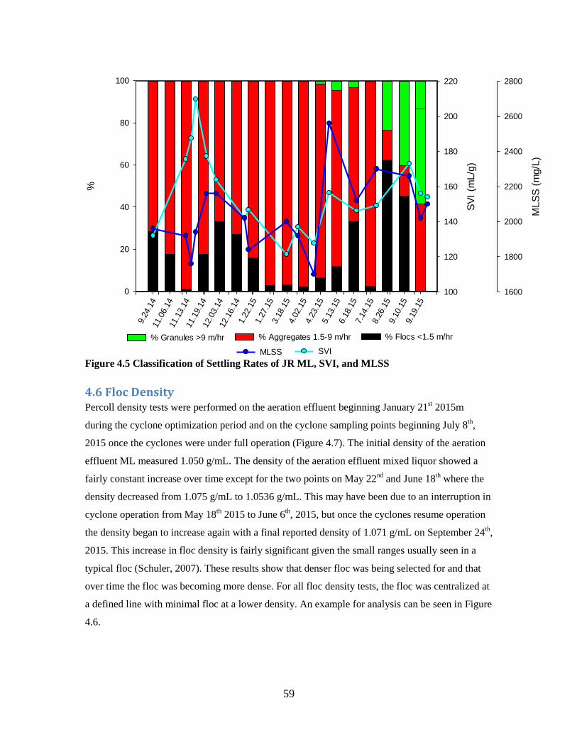
59
9.24
.14
11.0
6.14
11.1
3.14
11.1
9.14
12.0
3.14
12.1
6.14
1.22
.15
1.27
.15
3.18
.15
4.02
.15
4.23
.15
5.13
.15
6.18
.15
7.14
.15
8.26
.15
9.10
.15
9.19
.15
%
0
20
40
60
80
100
SV
I (m
L/g
)
100
120
140
160
180
200
220
MLS
S (
mg/L
)
1600
1800
2000
2200
2400
2600
2800
SVI MLSS
% Flocs <1.5 m/hr% Aggregates 1.5-9 m/hr% Granules >9 m/hr
Figure 4.5 Classification of Settling Rates of JR ML, SVI, and MLSS
4.6 Floc Density Percoll density tests were performed on the aeration effluent beginning January 21
st 2015m
during the cyclone optimization period and on the cyclone sampling points beginning July 8th,
2015 once the cyclones were under full operation (Figure 4.7). The initial density of the aeration
effluent ML measured 1.050 g/mL. The density of the aeration effluent mixed liquor showed a
fairly constant increase over time except for the two points on May 22nd
and June 18th where the
density decreased from 1.075 g/mL to 1.0536 g/mL. This may have been due to an interruption in
cyclone operation from May 18th 2015 to June 6
th, 2015, but once the cyclones resume operation
the density began to increase again with a final reported density of 1.071 g/mL on September 24th,
2015. This increase in floc density is fairly significant given the small ranges usually seen in a
typical floc (Schuler, 2007). These results show that denser floc was being selected for and that
over time the floc was becoming more dense. For all floc density tests, the floc was centralized at
a defined line with minimal floc at a lower density. An example for analysis can be seen in Figure
4.6.
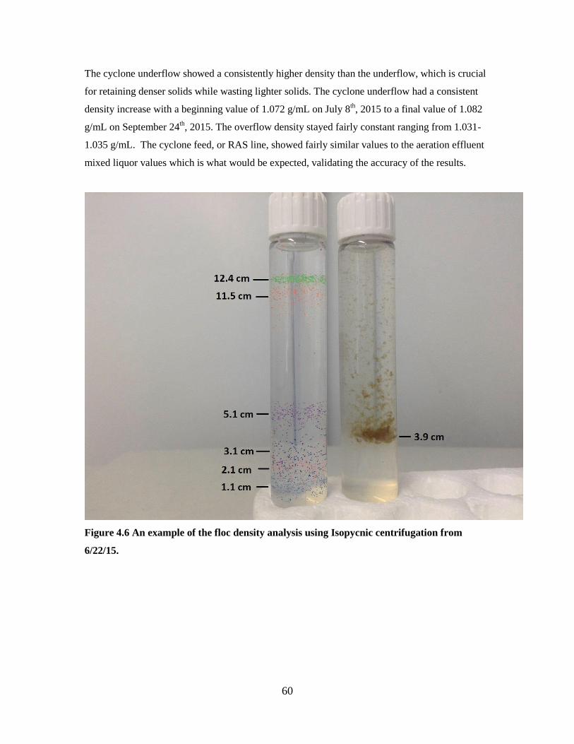
60
The cyclone underflow showed a consistently higher density than the underflow, which is crucial
for retaining denser solids while wasting lighter solids. The cyclone underflow had a consistent
density increase with a beginning value of 1.072 g/mL on July 8th, 2015 to a final value of 1.082
g/mL on September 24th, 2015. The overflow density stayed fairly constant ranging from 1.031-
1.035 g/mL. The cyclone feed, or RAS line, showed fairly similar values to the aeration effluent
mixed liquor values which is what would be expected, validating the accuracy of the results.
Figure 4.6 An example of the floc density analysis using Isopycnic centrifugation from
6/22/15.
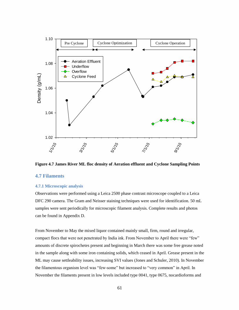
61
1/1/
15
3/1/
15
5/1/
15
7/1/
15
9/1/
15
De
nsity (
g/m
L)
1.02
1.04
1.06
1.08
1.10
Aeration Effluent
Underflow
Overflow
Cyclone Feed
Figure 4.7 James River ML floc density of Aeration effluent and Cyclone Sampling Points
4.7 Filaments
4.7.1 Microscopic analysis
Observations were performed using a Leica 2500 phase contrast microscope coupled to a Leica
DFC 290 camera. The Gram and Neisser staining techniques were used for identification. 50 mL
samples were sent periodically for microscopic filament analysis. Complete results and photos
can be found in Appendix D.
From November to May the mixed liquor contained mainly small, firm, round and irregular,
compact flocs that were not penetrated by India ink. From November to April there were “few”
amounts of discrete spirochetes present and beginning in March there was some free grease noted
in the sample along with some iron containing solids, which ceased in April. Grease present in the
ML may cause settleability issues, increasing SVI values (Jones and Schuler, 2010). In November
the filamentous organism level was “few-some” but increased to “very common” in April. In
November the filaments present in low levels included type 0041, type 0675, nocardioforms and
Pre Cyclone Cyclone Optimization Cyclone Operation
62
type 1701 and in March the filaments present in small amounts included type 1863, H
Hydrossis, nocardioforms and type 1701, none of these sufficient enough to interfere with the
settleability of the sludge. In April and May nocardioform was noticed as the main filamentous
organism, present in the sludge floc and free in the solution. Nocardioform abundance was seen at
levels that would result in foaming. In April other filaments present at levels too low to interfere
with settling included type 1863, H Hydrossis, Thiothrix and type 1701. In May only minor
amounts of H Hydrossis and type 1701 were noted. In June, when the cyclones were started up
again after a 3 week shut down, the overall filamentous organism level decreased to was "some"
which is not sufficient to interfere with settling. In June the filaments were all present in small
amounts; they were nocardioforms, type 0041 and type 0675.
These results indicate the filamentous organisms are being selected against; only the ones inside
the floc or slightly protruding were present in the June sample. Presence of nocardioforms may
have been due to recycling and trapping in the activated sludge and therefore would be immune
from a “selection strategy” based on dense, settling biomass.
Initial samples were sent for analysis in October 2014 and throughout the entire study the flocs
contained large amounts of PAO bacteria and no GAO bacteria. However in November some
GAO bacteria was present, but upon analysis of the next sample, no GAO bacteria was found.
The PAO bacteria were present as large grape-like clusters of coccoid cells and clusters of small
coccoid cells. It is not clear whether these are two separate types of PAO bacteria or just different
morphological forms of the same organism. In April the level of small coccoid cells increased
over the previous sample.
4.7.2 Plant Data
Historical data for the JR plant has not shown a correlation between seasonal variations and
filament abundance. Filament abundance from 2014-2015 can be found in Appendix D with
values never reaching that of nuisance levels. The primary filament type was Nocardioforms.
Other filament types included 0041, 0875, and Thiothrix II.
4.8 PAO Activity Tests
PAO Activity tests provide results for:
Determining amount of PAO and DPAO activity from the phosphate release rate
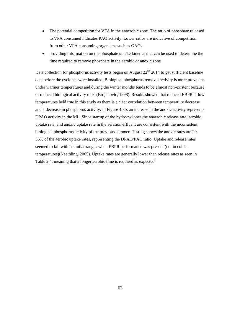
63
The potential competition for VFA in the anaerobic zone. The ratio of phosphate released
to VFA consumed indicates PAO activity. Lower ratios are indicative of competition
from other VFA consuming organisms such as GAOs
providing information on the phosphate uptake kinetics that can be used to determine the
time required to remove phosphate in the aerobic or anoxic zone
Data collection for phosphorus activity tests began on August 22nd
2014 to get sufficient baseline
data before the cyclones were installed. Biological phosphorus removal activity is more prevalent
under warmer temperatures and during the winter months tends to be almost non-existent because
of reduced biological activity rates (Brdjanovic, 1998). Results showed that reduced EBPR at low
temperatures held true in this study as there is a clear correlation between temperature decrease
and a decrease in phosphorus activity. In Figure 4.8b, an increase in the anoxic activity represents
DPAO activity in the ML. Since startup of the hydrocyclones the anaerobic release rate, aerobic
uptake rate, and anoxic uptake rate in the aeration effluent are consistent with the inconsistent
biological phosphorus activity of the previous summer. Testing shows the anoxic rates are 29-
56% of the aerobic uptake rates, representing the DPAO/PAO ratio. Uptake and release rates
seemed to fall within similar ranges when EBPR performance was present (not in colder
temperatures)(Neethling, 2005). Uptake rates are generally lower than release rates as seen in
Table 2.4, meaning that a longer aerobic time is required as expected.
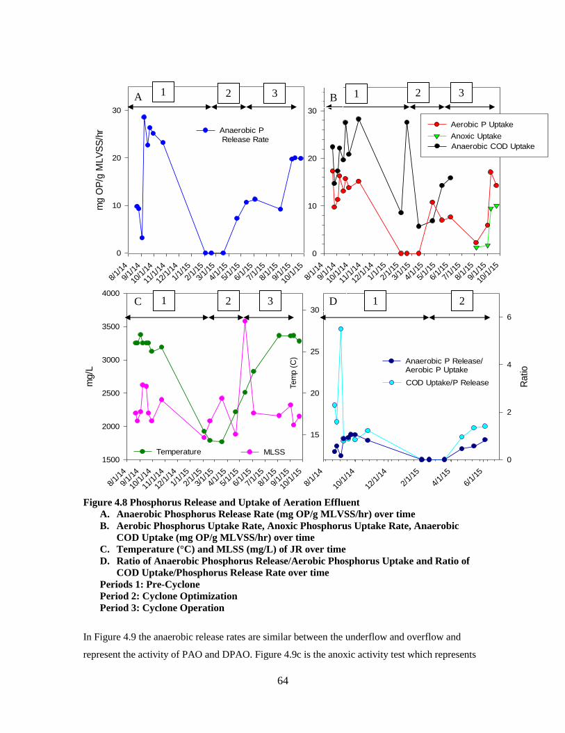
64
8/1/
14
9/1/
14
10/1
/14
11/1
/14
12/1
/14
1/1/
15
2/1/
15
3/1/
15
4/1/
15
5/1/
15
6/1/
15
7/1/
15
8/1/
15
9/1/
15
10/1
/15
mg O
P/g
MLV
SS
/hr
0
10
20
30
8/1/
14
9/1/
14
10/1
/14
11/1
/14
12/1
/14
1/1/
15
2/1/
15
3/1/
15
4/1/
15
5/1/
15
6/1/
15
7/1/
15
8/1/
15
9/1/
15
10/1
/15
0
10
20
30
8/1/
14
10/1
/14
12/1
/14
2/1/
15
4/1/
15
6/1/
15
Ratio
0
2
4
6
8/1/
14
9/1/
14
10/1
/14
11/1
/14
12/1
/14
1/1/
15
2/1/
15
3/1/
15
4/1/
15
5/1/
15
6/1/
15
7/1/
15
8/1/
15
9/1/
15
10/1
/15
mg/L
1500
2000
2500
3000
3500
4000Tem
p (
C)
15
20
25
30
COD Uptake/P Release
Anaerobic P Release/ Aerobic P Uptake
MLSSTemperature
Anaerobic P
Release RateAnaerobic COD Uptake
Aerobic P Uptake
Anoxic Uptake
Anaerobic COD Uptake
Aerobic P Uptake
Anoxic Uptake
Figure 4.8 Phosphorus Release and Uptake of Aeration Effluent
A. Anaerobic Phosphorus Release Rate (mg OP/g MLVSS/hr) over time
B. Aerobic Phosphorus Uptake Rate, Anoxic Phosphorus Uptake Rate, Anaerobic
COD Uptake (mg OP/g MLVSS/hr) over time
C. Temperature (°C) and MLSS (mg/L) of JR over time
D. Ratio of Anaerobic Phosphorus Release/Aerobic Phosphorus Uptake and Ratio of
COD Uptake/Phosphorus Release Rate over time
Periods 1: Pre-Cyclone
Period 2: Cyclone Optimization
Period 3: Cyclone Operation
In Figure 4.9 the anaerobic release rates are similar between the underflow and overflow and
represent the activity of PAO and DPAO. Figure 4.9c is the anoxic activity test which represents
1 3 2
1
1
2 1
2 3
3 2
A
C
B
D
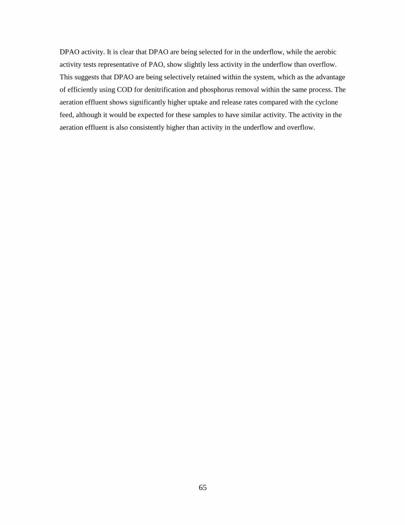
65
DPAO activity. It is clear that DPAO are being selected for in the underflow, while the aerobic
activity tests representative of PAO, show slightly less activity in the underflow than overflow.
This suggests that DPAO are being selectively retained within the system, which as the advantage
of efficiently using COD for denitrification and phosphorus removal within the same process. The
aeration effluent shows significantly higher uptake and release rates compared with the cyclone
feed, although it would be expected for these samples to have similar activity. The activity in the
aeration effluent is also consistently higher than activity in the underflow and overflow.
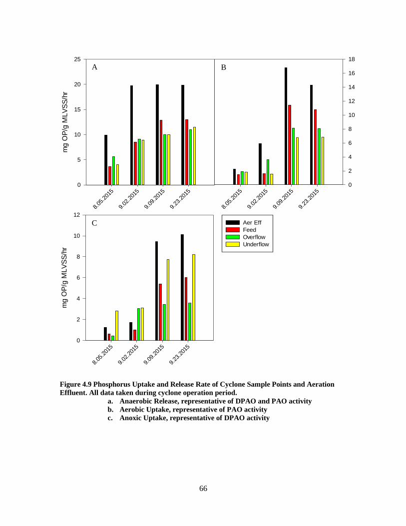
66
8.05
.201
5
9.02
.201
5
9.09
.201
5
9.23
.201
5
mg O
P/g
MLV
SS
/hr
0
5
10
15
20
25
Aer Eff
Feed
Overflow
Underflow
8.05
.201
5
9.02
.201
5
9.09
.201
5
9.23
.201
50
2
4
6
8
10
12
14
16
18
8.05
.201
5
9.02
.201
5
9.09
.201
5
9.23
.201
5
mg O
P/g
MLV
SS
/hr
0
2
4
6
8
10
12
Figure 4.9 Phosphorus Uptake and Release Rate of Cyclone Sample Points and Aeration
Effluent. All data taken during cyclone operation period.
a. Anaerobic Release, representative of DPAO and PAO activity
b. Aerobic Uptake, representative of PAO activity
c. Anoxic Uptake, representative of DPAO activity
A B
C
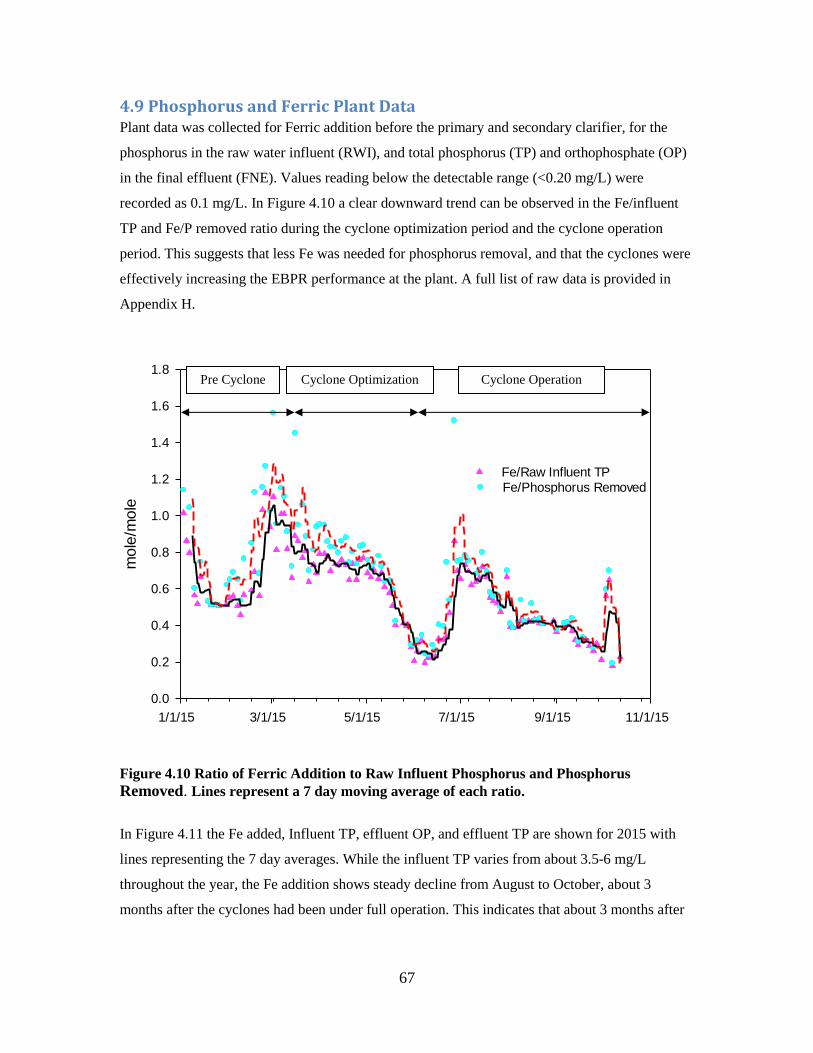
67
4.9 Phosphorus and Ferric Plant Data Plant data was collected for Ferric addition before the primary and secondary clarifier, for the
phosphorus in the raw water influent (RWI), and total phosphorus (TP) and orthophosphate (OP)
in the final effluent (FNE). Values reading below the detectable range (<0.20 mg/L) were
recorded as 0.1 mg/L. In Figure 4.10 a clear downward trend can be observed in the Fe/influent
TP and Fe/P removed ratio during the cyclone optimization period and the cyclone operation
period. This suggests that less Fe was needed for phosphorus removal, and that the cyclones were
effectively increasing the EBPR performance at the plant. A full list of raw data is provided in
Appendix H.
1/1/15 3/1/15 5/1/15 7/1/15 9/1/15 11/1/15
mole
/mole
0.0
0.2
0.4
0.6
0.8
1.0
1.2
1.4
1.6
1.8
Fe/Raw Influent TPFe/Phosphorus Removed
Figure 4.10 Ratio of Ferric Addition to Raw Influent Phosphorus and Phosphorus
Removed. Lines represent a 7 day moving average of each ratio.
In Figure 4.11 the Fe added, Influent TP, effluent OP, and effluent TP are shown for 2015 with
lines representing the 7 day averages. While the influent TP varies from about 3.5-6 mg/L
throughout the year, the Fe addition shows steady decline from August to October, about 3
months after the cyclones had been under full operation. This indicates that about 3 months after
Pre Cyclone Cyclone Optimization Cyclone Operation
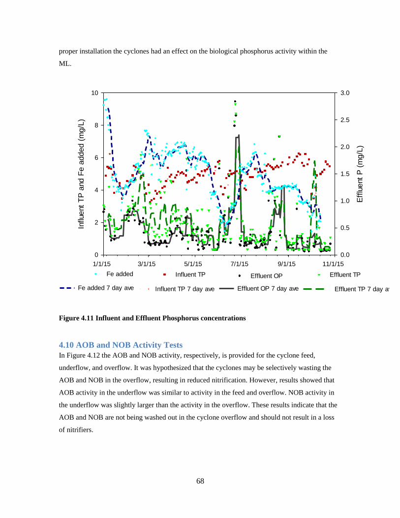
68
proper installation the cyclones had an effect on the biological phosphorus activity within the
ML.
1/1/15 3/1/15 5/1/15 7/1/15 9/1/15 11/1/15
Influent
TP
and F
e a
dded (
mg/L
)
0
2
4
6
8
10
Eff
luent
P (
mg/L
)
0.0
0.5
1.0
1.5
2.0
2.5
3.0
Influent TP
Influent TP 7 day ave
Effluent OP
Effluent OP 7 day ave
Effluent TP
Effluent TP 7 day ave
Fe added
Fe added 7 day ave
Figure 4.11 Influent and Effluent Phosphorus concentrations
4.10 AOB and NOB Activity Tests
In Figure 4.12 the AOB and NOB activity, respectively, is provided for the cyclone feed,
underflow, and overflow. It was hypothesized that the cyclones may be selectively wasting the
AOB and NOB in the overflow, resulting in reduced nitrification. However, results showed that
AOB activity in the underflow was similar to activity in the feed and overflow. NOB activity in
the underflow was slightly larger than the activity in the overflow. These results indicate that the
AOB and NOB are not being washed out in the cyclone overflow and should not result in a loss
of nitrifiers.
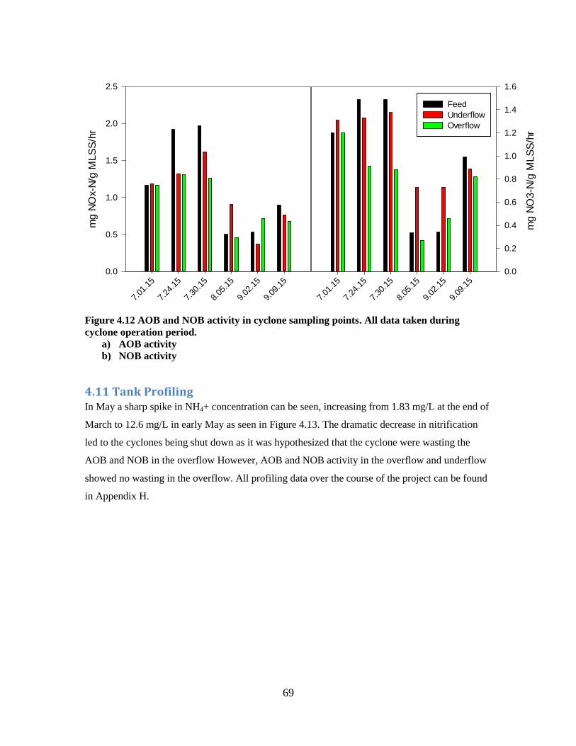
69
7.01
.15
7.24
.15
7.30
.15
8.05
.15
9.02
.15
9.09
.15
mg N
O3-N
/g M
LS
S/h
r
0.0
0.2
0.4
0.6
0.8
1.0
1.2
1.4
1.6
Feed
Underflow
Overflow
7.01
.15
7.24
.15
7.30
.15
8.05
.15
9.02
.15
9.09
.15
mg N
Ox-
N/g
MLS
S/h
r
0.0
0.5
1.0
1.5
2.0
2.5
Figure 4.12 AOB and NOB activity in cyclone sampling points. All data taken during
cyclone operation period. a) AOB activity
b) NOB activity
4.11 Tank Profiling In May a sharp spike in NH4+ concentration can be seen, increasing from 1.83 mg/L at the end of
March to 12.6 mg/L in early May as seen in Figure 4.13. The dramatic decrease in nitrification
led to the cyclones being shut down as it was hypothesized that the cyclone were wasting the
AOB and NOB in the overflow However, AOB and NOB activity in the overflow and underflow
showed no wasting in the overflow. All profiling data over the course of the project can be found
in Appendix H.
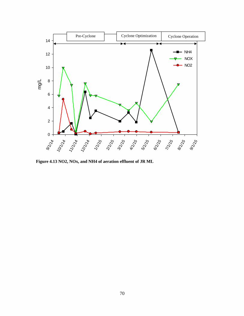
70
9/1/
14
10/1
/14
11/1
/14
12
/1/1
4
1/1/
15
2/1/
15
3/1/
15
4/1/
15
5/1/
15
6/1/
15
7/1/
15
8/1/
15
9/1/
15
mg/L
0
2
4
6
8
10
12
14
NH4
NO2
NOX
Figure 4.13 NO2, NOx, and NH4 of aeration effluent of JR ML
Pre-Cyclone Cyclone Optimization Cyclone Operation
71
5. Conclusions and engineering significance Preliminary conclusions can be made about the effects of hydrocyclones on the settleability and
enhanced biological phosphorus removal applied to the mainstream of a wastewater treatment
plant. Biological phosphorus removal activity was present in the wastewater at similar rates when
comparing the period before and after hydrocyclones were installed, indicating that the
hydrocyclones may not have had an effect on the biological phosphorus activity, which may have
been due to the short period they were fully operational. However, it was noted that anoxic
biological phosphorus activity was increasing over time indicating that DPAO were being
selectively retained.
AOB and NOB activity measurements in the cyclone overflow, underflow, and feed indicated
that nitrifiers were not being selectively wasted from the system, indicating that nitrification at
the plant should not be affected by the hydrocyclones. Filament data taken from the plant and
microscopic analysis showed that some filaments were present in the system but not at levels that
would hinder settleability or cause foaming, which showed that filamentous organisms were
being selected against. It was also shown through filamentous analysis that PAO were present
while the GAO population was minimal. The floc density of the aeration effluent mixed liquor
was shown to increase steadily over time from 1.050-1.071 g/mL. The density of the cyclone
overflow and underflow showed a large difference in density, which meant that the denser sludge
was being selectively retained while wasting the lighter sludge. Over time, the settleability would
increase with the retention of denser sludge. Plant data collected for James River does suggest a
reduction in Ferric as biological phosphorus removal remained constant during the last 2 months
of data collection. A reduction in Ferric addition was noticed about 3 months after the cyclones
were under full operation, indicating an increase in biological phosphorus activity. ISV tests show
that the cyclone underflow has a much higher settling velocity than the cyclone overflow. The
cyclone feed ISV did not increase over time but data was taken over a period slightly less than
three months which may not have been enough time for a noticeable effect. 2015 SVI data shows
a slight decrease in the average SVI5 decreasing from 292 mL/g to 248 mL/g after cyclones were
installed, while the SVI30 value remained fairly constant. SVI is slow to change as it is more
representative of the total floc structure, but as granules within the system become more stable, a
decrease in SVI and increase ISV data should be observed. Solids flux data showed an increase in
initial settling velocity from the pre-cyclone to cyclone optimization period and then again during
the cyclone operation period. Vesilind values indicate an increase in Vo while k showed a
minimal decrease, both indicating better settleability characteristics. Classification of settleability
72
rate data indicated that granule percentage increased from 0% during the pre-cyclone period to up
to 24-40% during the cyclone operation period. Pilot scale studies demonstrated that it took about
1-3 months for full granulation so it may be that in a full-scale study it would take longer to
achieve the same results due to the large volume of ML. The floc fraction showed a large increase
from the pre-cyclone and cyclone optimization to the cyclone operation period with averages
increasing from 14±11% to 37±22%. The aggregate percentage was the majority of the floc
characterization during pre-cyclone and cyclone optimization periods averaging 86±11% and
decreasing to 47±35%. It is unclear why the aggregate percentage decreased as the floc and
granule percentages had such a high increase.
Wastewater treatment plants all over the world suffer from settleability issues, while also needing
to meet increasingly stringent nutrient limits. Settleability is often a limiting step of the
wastewater treatment process. Poor settleability may results in a high TSS effluent or a high
nutrient concentration in the effluent which can lead to eutrophication in receiving water bodies.
Aerobic granular sludge research has indicated the multiple benefits that it can achieve in a
wastewater system by increasing settling rates through superior settling characteristics while
removing nutrients in a single system through stratified layers. Using an external selector to
achieve biological phosphorus or stabilize erratic biological phosphorus removal is significant in
that most wastewater treatment plants cannot do this without the use of an anaerobic selector.
This has the potential to apply external selectors to existing infrastructure throughout plants
worldwide to achieve not only biological phosphorus removal, but also improved settleability
with a very minor capital investment.
73
References Acevedo, B., Borras, L., Oehmen, A., & Barat, R. (2014). Modelling the metabolic shift
of polyphosphate-accumulating organisms. Water Research, 65, 235-244. doi:
http://dx.doi.org/10.1016/j.watres.2014.07.028
Ahn, J.; Daidou, T.; Tsuneda, S.; Hirata, A. (2002). Characterization of denitrifying
phosphate-accumulating organisms cultivated under different electron acceptor
conditions using polymerase chain reaction-denaturing gradient gelel
ectrophoresis assay. Water Research, 36.
Carvalho, G.; Lemos, P.; Oehmen, A.; Reis, M. (2007). Denitrifying phosphorus
removal: Linking the process performance with the microbial community
structure. Water Research, 41.
Carvalheira, M., Oehmen, A., Carvalho, G., Eusébio, M., & Reis, M. A. M. (2014). The
impact of aeration on the competition between polyphosphate accumulating
organisms and glycogen accumulating organisms. Water Research, 66(0), 296-
307. doi: http://dx.doi.org/10.1016/j.watres.2014.08.033
Carvalheira, M., Oehmen, A., Carvalho, G., & Reis, M. A. M. (2014). Survival strategies
of polyphosphate accumulating organisms and glycogen accumulating organisms
under conditions of low organic loading. Bioresource Technology, 172(0), 290-
296. doi: http://dx.doi.org/10.1016/j.biortech.2014.09.059
Cell Separation Media Methodology and Applications. (1985). In G. H. L. Sciences
(Ed.): General Electric Company.
Chudoba, J.; Cech, J. S.; Farkac, J.; Grau, P. . (1985). Control of Activated Sludge
Filamentous Bulking: Experimental Verification of a Kinetic Selection Theory.
Water Research, 191-196.
de Kreuk, M. K. (2006). Aerobic Granular Sludge Scaling up a new technology.
de Kreuk, M. K., de Kreuk, M., Heijnen, J. J., & van Loosdrecht, M. C. M. (2005).
Simultaneous COD, nitrogen, and phosphate removal by aerobic granular sludge.
Biotechnology and bioengineering, 90(6), 761-769.
Denny Parker, George Ekama, Henryk Melcer, Andre van Niekirk, Dean M. Shiskowski,
David J. L. Forgie, W. L. Marten, G. T. Daigger. (1998). Full-Scale Evaluation of
Factors Affecting the Performance of Anoxic Selectors. Water Environment
Research, 70(6), 1225-1231.
Ekama, G.A.; Barnard, J. L.; Günthert, F. W.; Krebs, P.; McCorquodale, J. A.; Parker, D.
S.; Wahlberg, E. J. . (2006). Secondary Settling Tanks Scientific and Technical
Report (Vol. 6). London, UK: IWA.
EnviroSim Associates, LTD. (2014). BioWin 4.0 (Version 4).
Gao, D. W., Liu, L., Liang, H., & Wu, W. M. (2011). Aerobic granular sludge:
characterization, mechanism of granulation and application to wastewater
treatment. Critical Reviews in Biotechnology, 31(2), 137-152. doi:
10.3109/07388551.2010.497961
Grady, C. P. Leslie et al. (2011). Biological Wastewater Treatment (Vol. 19). Boca
Raton, FL: IWA Pub./CRC Press.
Houweling, D.; Constantine, T.; Sandino, S.; Neilson, P. H.; Uri N.; Havsteen L. (2015).
What the Cyclone did to my Sludge and Other Tales of Activated Sludge
Granulation. Water Environment Association of Ontario. Toronto, Ontario,
Canada.
74
J. Chudoba, P. Grau, V. Ottova. (1973). Control of Activated-Sludge Filamentous
Bulking- II. Selection of Microorganisms by Means of a Selector. Water
Research, 7, 1389-1406.
Jenkins, D.; Richard, M. G.; Daigger, G. T. (2003). Manual on the Causes and Control
of Activated Sludge Bulking, Foaming and Other Solids Separaton Problems:
Lewis Publishers.
Jones, Patricia A., & Schuler, Andrew J. (2010). Seasonal variability of biomass density
and activated sludge settleability in full-scale wastewater treatment systems.
Chemical Engineering Journal, 164(1), 16-22.
Kim, Hyun-su, Gellner, James W., Boltz, Joshua P., Freudenberg, Robert G., Gunsch,
Claudia K., & Schuler, Andrew J. (2010). Effects of integrated fixed film
activated sludge media on activated sludge settling in biological nutrient removal
systems. Water Research, 44(5), 1553-1561.
Kuba, T., van Loosdrecht, M.C.M., Heijnen, J.J. Phosphorus and nitrogen removal with
minimal COD requirement by integration of denitrifying dephosphatation and
nitrification in a two-sludge system, Water Research, Volume 30, Issue 7, July
1996, Pages 1702-1710, ISSN 0043-1354
Liu, Y., Wang, Z., Qin, L., Liu, T., Tay, J. (2004). Selection pressure-driven aerobic
granulation in a sequencing batch reactor. Applied Microbiology and
Biotechnology.
Lopez-Vazquez, C. M.; Oehmen, A.; Hooijmans, C. M.; Brdjanovic, D.; Gijzen, H. J.;
Yuan, Z.; van Loosdrecht, M. C. M. (2009). Modeling the PAO–GAO
competition: Effects of carbon source, pH and temperature. Water Research,
43(2), 450-462. doi: http://dx.doi.org/10.1016/j.watres.2008.10.032
Mancell-Egala, A. (2014). Protocols for Settleability.
Martins, António M. P., Pagilla, Krishna, Heijnen, Joseph J., & van Loosdrecht, Mark C.
M. (2004). Filamentous bulking sludge—a critical review. Water Research, 38(4),
793-817. doi: http://dx.doi.org/10.1016/j.watres.2003.11.005
Metcalf, Eddy. (2014). Wastewater Engineering Treatment and Resource Recovery:
McGraw-Hill Education.
Mishima, K., & Nakamura, M. (1991). Self-Immobilization of Aerobic Activated Sludge-
-A Pilot Study of the Aerobic Upflow Sludge Blanket Process in Municipal
Sewage Treatment. Water Science and Technology, 23, 981-990.
Morgenroth E.; Sherden, T.; Van Loosdrecht, M. C. M.; Heijnen, J. J.; Wilderer, P. A. .
(1997). Aerobic Granular Sludge in a Sequencing Batch Reactor. Water Research,
31(12), 3.
Neethling, J. B.; Bakke, B.; Benisch, M.; Gu, A.; Stephens, H.; Stensel, H. D.; Moore,
R. (2005). Factors Influencing the Reliability of Enhanced Biological Phosphorus
Removal. In WERF (Ed.).
Nyhuis, Geert. (2013). Switzerland Patent No.: U. S. P. A. Publication.
Oehmen, A., Carvalho, G., Lopez-Vazquez, C. M., van Loosdrecht, M. C. M., & Reis, M.
A. M. (2010). Incorporating microbial ecology into the metabolic modelling of
polyphosphate accumulating organisms and glycogen accumulating organisms.
Water Research, 44(17), 4992-5004. doi:
http://dx.doi.org/10.1016/j.watres.2010.06.071
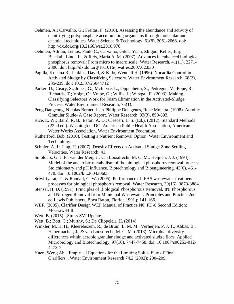
75
Oehmen, A.; Carvalho, G.; Freitas, F. (2010). Assessing the abundance and activity of
denitrifying polyphosphate accumulating organisms through molecular and
chemical techniques. Water Science & Technology, 61(8), 2061-2068. doi:
http://dx.doi.org/10.2166/wst.2010.976
Oehmen, Adrian, Lemos, Paulo C., Carvalho, Gilda, Yuan, Zhiguo, Keller, Jürg,
Blackall, Linda L., & Reis, Maria A. M. (2007). Advances in enhanced biological
phosphorus removal: From micro to macro scale. Water Research, 41(11), 2271-
2300. doi: http://dx.doi.org/10.1016/j.watres.2007.02.030
Pagilla, Krishna R., Jenkins, David, & Kido, Wendell H. (1996). Nocardia Control in
Activated Sludge by Classifying Selectors. Water Environment Research, 68(2),
235-239. doi: 10.2307/25044712
Parker, D.; Geary, S.; Jones, G.; McIntyre, L.; Oppenheim, S.; Pedregon, V.; Pope, R.;
Richards, T.; Voigt, C.; Volpe, G.; Willis, J.; Witzgall R. (2003). Making
Classifying Selectors Work for Foam Elimination in the Activated-Sludge
Process. Water Environment Research, 75(1).
Peng Dangcong, Nicolas Bernet, Jean-Philippe Delegenes, Rene Moletta. (1998). Aerobic
Granular Slude- A Case Report. Water Research, 33(3), 890-893.
Rice, E. W.; Baird, R. B.; Eaton, A. D.; Clesceri, L. S. (Ed.). (2012). Standard Methods
(22nd ed.). Washington, DC: American Public Health Association, American
Water Works Association, Water Environment Federation.
Rutherford, Bob. (2010). Testing a Nutrient Removal Option. Water Environment and
Technolohy.
Schuler, A. J.; Jang, H. (2007). Density Effects on Activated Sludge Zone Settling
Velocities. Water Research, 41.
Smolders, G. J. F.; van der Meij, J.; van Loosdrecht, M. C. M.; Heijnen, J. J. (1994).
Model of the anaerobic metabolism of the biological phosphorus removal process:
Stoichiometry and pH influence. Biotechnology and Bioengineering, 43(6), 461-
470. doi: 10.1002/bit.260430605
Sriwiriyarat, T., & Randall, C. W. (2005). Performance of IFAS wastewater treatment
processes for biological phosphorus removal. Water Research, 39(16), 3873-3884.
Stensel, H. D. (1991). Principles of Biological Phosphorous Removal. IN: Phosphorous
and Nitrogen Removal from Municipal Wastewater: Principles and Practice.2nd
ed.Lewis Publishers, Boca Raton, Florida.1991.p 141-166.
WEF. (2005). Clarifier Design WEF Manual of Practice N0. FD-8 Second Edition:
McGraw-Hill.
Wett, B. (2015). [Strass SVI Update].
Wett, B.; Bott, C.; Murthy, S.; De Clippeleir, H. (2014).
Winkler, M. K. H., Kleerebezem, R., de Bruin, L. M. M., Verheijen, P. J. T., Abbas, B.,
Habermacher, J., & van Loosdrecht, M. C. M. (2013). Microbial diversity
differences within aerobic granular sludge and activated sludge flocs. Applied
Microbiology and Biotechnology, 97(16), 7447-7458. doi: 10.1007/s00253-012-
4472-7
Yuen, Weng Ah. “Empirical Equations for the Limiting Solids Flux of Final
Clarifiers”. Water Environment Research 74.2 (2002): 200–209.
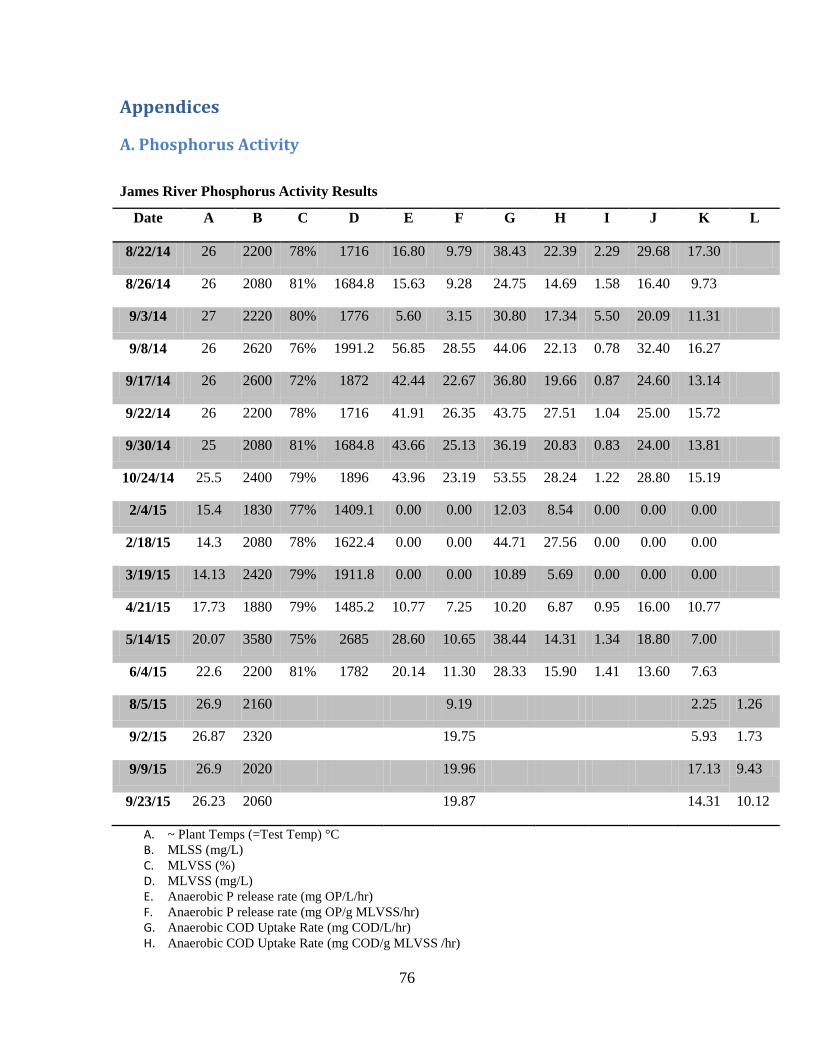
76
Appendices
A. Phosphorus Activity
James River Phosphorus Activity Results
Date A B C D E F G H I J K L
8/22/14 26 2200 78% 1716 16.80 9.79 38.43 22.39 2.29 29.68 17.30
8/26/14 26 2080 81% 1684.8 15.63 9.28 24.75 14.69 1.58 16.40 9.73
9/3/14 27 2220 80% 1776 5.60 3.15 30.80 17.34 5.50 20.09 11.31
9/8/14 26 2620 76% 1991.2 56.85 28.55 44.06 22.13 0.78 32.40 16.27
9/17/14 26 2600 72% 1872 42.44 22.67 36.80 19.66 0.87 24.60 13.14
9/22/14 26 2200 78% 1716 41.91 26.35 43.75 27.51 1.04 25.00 15.72
9/30/14 25 2080 81% 1684.8 43.66 25.13 36.19 20.83 0.83 24.00 13.81
10/24/14 25.5 2400 79% 1896 43.96 23.19 53.55 28.24 1.22 28.80 15.19
2/4/15 15.4 1830 77% 1409.1 0.00 0.00 12.03 8.54 0.00 0.00 0.00
2/18/15 14.3 2080 78% 1622.4 0.00 0.00 44.71 27.56 0.00 0.00 0.00
3/19/15 14.13 2420 79% 1911.8 0.00 0.00 10.89 5.69 0.00 0.00 0.00
4/21/15 17.73 1880 79% 1485.2 10.77 7.25 10.20 6.87 0.95 16.00 10.77
5/14/15 20.07 3580 75% 2685 28.60 10.65 38.44 14.31 1.34 18.80 7.00
6/4/15 22.6 2200 81% 1782 20.14 11.30 28.33 15.90 1.41 13.60 7.63
8/5/15 26.9 2160 9.19 2.25 1.26
9/2/15 26.87 2320 19.75 5.93 1.73
9/9/15 26.9 2020 19.96 17.13 9.43
9/23/15 26.23 2060 19.87 14.31 10.12
A. ~ Plant Temps (=Test Temp) °C
B. MLSS (mg/L)
C. MLVSS (%)
D. MLVSS (mg/L)
E. Anaerobic P release rate (mg OP/L/hr)
F. Anaerobic P release rate (mg OP/g MLVSS/hr)
G. Anaerobic COD Uptake Rate (mg COD/L/hr)
H. Anaerobic COD Uptake Rate (mg COD/g MLVSS /hr)

77
I. COD uptake : P Release (RATIO)
J. Aerobic P uptake rate (mg OP/L/hr)
K. Aerobic P uptake rate (mg OP/g MLVSS /hr)
L. Anoxic Uptake rate (mg OP/g MLVSS /hr)
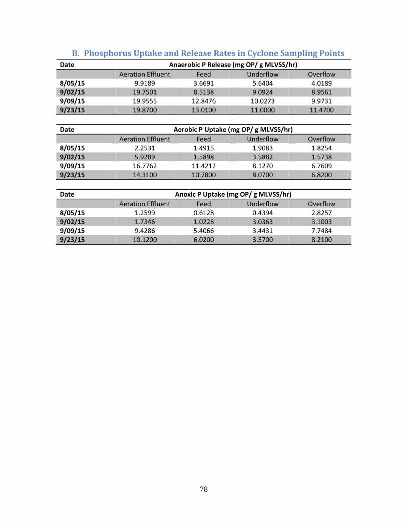
78
B. Phosphorus Uptake and Release Rates in Cyclone Sampling Points
Date Anaerobic P Release (mg OP/ g MLVSS/hr)
Aeration Effluent Feed Underflow Overflow 8/05/15 9.9189 3.6691 5.6404 4.0189 9/02/15 19.7501 8.5138 9.0924 8.9561 9/09/15 19.9555 12.8476 10.0273 9.9731 9/23/15 19.8700 13.0100 11.0000 11.4700
Date Aerobic P Uptake (mg OP/ g MLVSS/hr)
Aeration Effluent Feed Underflow Overflow 8/05/15 2.2531 1.4915 1.9083 1.8254 9/02/15 5.9289 1.5898 3.5882 1.5738 9/09/15 16.7762 11.4212 8.1270 6.7609 9/23/15 14.3100 10.7800 8.0700 6.8200
Date Anoxic P Uptake (mg OP/ g MLVSS/hr)
Aeration Effluent Feed Underflow Overflow 8/05/15 1.2599 0.6128 0.4394 2.8257 9/02/15 1.7346 1.0228 3.0363 3.1003 9/09/15 9.4286 5.4066 3.4431 7.7484 9/23/15 10.1200 6.0200 3.5700 8.2100
79
C. AOB and NOB Activity in Cyclone Sampling Points
Date AOB NOB
Feed Underflow Overflow Feed Underflow Overflow
7/14/15 1.1681 1.1851 1.1681 1.2007 1.3085 1.2007
7/24/15 1.9200 1.3221 1.3100 1.4900 1.3300 0.9100
7/30/15 1.9684 1.6166 1.2628 1.4889 1.3752 0.8787
8/05/15 0.4995 0.9084 0.4603 0.3339 0.7281 0.2689
9/02/15 0.5300 0.3695 0.7200 0.3400 0.7300 0.4600
9/09/15 0.8950 0.7616 0.6809 0.9890 0.8869 0.8222
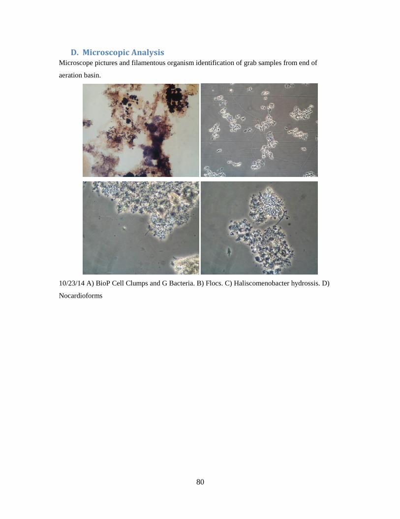
80
D. Microscopic Analysis Microscope pictures and filamentous organism identification of grab samples from end of
aeration basin.
10/23/14 A) BioP Cell Clumps and G Bacteria. B) Flocs. C) Haliscomenobacter hydrossis. D)
Nocardioforms
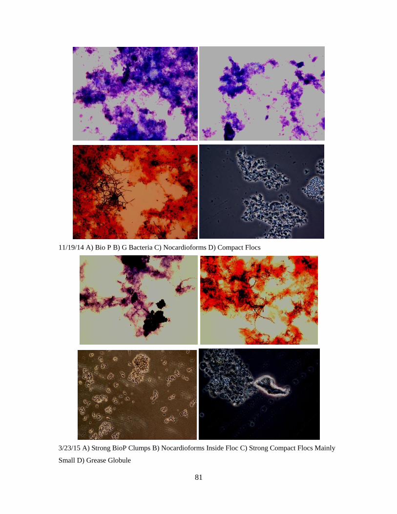
81
11/19/14 A) Bio P B) G Bacteria C) Nocardioforms D) Compact Flocs
3/23/15 A) Strong BioP Clumps B) Nocardioforms Inside Floc C) Strong Compact Flocs Mainly
Small D) Grease Globule
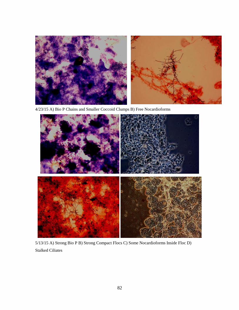
82
4/23/15 A) Bio P Chains and Smaller Coccoid Clumps B) Free Nocardioforms
5/13/15 A) Strong Bio P B) Strong Compact Flocs C) Some Nocardioforms Inside Floc D)
Stalked Ciliates
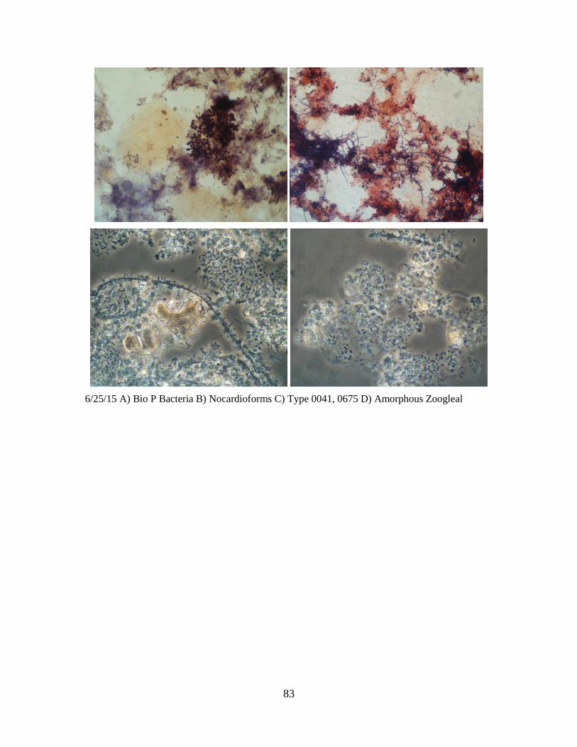
83
6/25/15 A) Bio P Bacteria B) Nocardioforms C) Type 0041, 0675 D) Amorphous Zoogleal
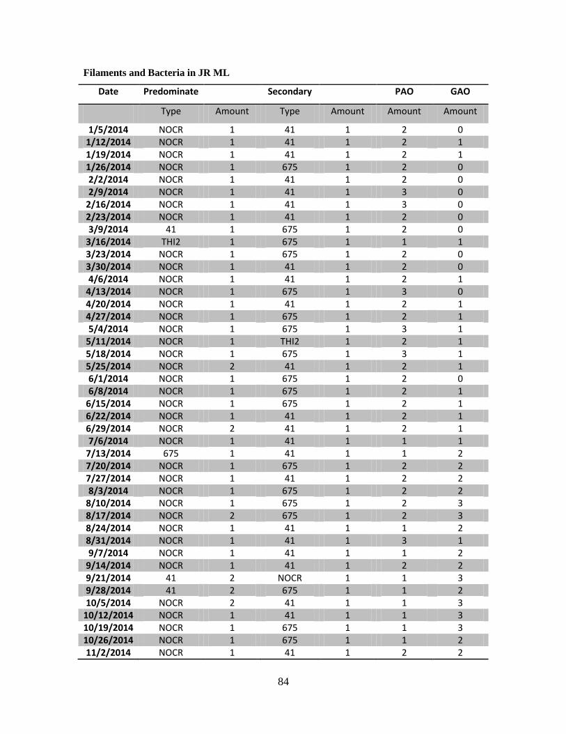
84
Filaments and Bacteria in JR ML
Date Predominate Secondary PAO GAO
Type Amount Type Amount Amount Amount
1/5/2014 NOCR 1 41 1 2 0 1/12/2014 NOCR 1 41 1 2 1 1/19/2014 NOCR 1 41 1 2 1 1/26/2014 NOCR 1 675 1 2 0 2/2/2014 NOCR 1 41 1 2 0 2/9/2014 NOCR 1 41 1 3 0
2/16/2014 NOCR 1 41 1 3 0 2/23/2014 NOCR 1 41 1 2 0 3/9/2014 41 1 675 1 2 0
3/16/2014 THI2 1 675 1 1 1 3/23/2014 NOCR 1 675 1 2 0 3/30/2014 NOCR 1 41 1 2 0 4/6/2014 NOCR 1 41 1 2 1
4/13/2014 NOCR 1 675 1 3 0 4/20/2014 NOCR 1 41 1 2 1 4/27/2014 NOCR 1 675 1 2 1 5/4/2014 NOCR 1 675 1 3 1
5/11/2014 NOCR 1 THI2 1 2 1 5/18/2014 NOCR 1 675 1 3 1 5/25/2014 NOCR 2 41 1 2 1 6/1/2014 NOCR 1 675 1 2 0 6/8/2014 NOCR 1 675 1 2 1
6/15/2014 NOCR 1 675 1 2 1 6/22/2014 NOCR 1 41 1 2 1 6/29/2014 NOCR 2 41 1 2 1 7/6/2014 NOCR 1 41 1 1 1
7/13/2014 675 1 41 1 1 2 7/20/2014 NOCR 1 675 1 2 2 7/27/2014 NOCR 1 41 1 2 2 8/3/2014 NOCR 1 675 1 2 2
8/10/2014 NOCR 1 675 1 2 3 8/17/2014 NOCR 2 675 1 2 3 8/24/2014 NOCR 1 41 1 1 2 8/31/2014 NOCR 1 41 1 3 1 9/7/2014 NOCR 1 41 1 1 2
9/14/2014 NOCR 1 41 1 2 2 9/21/2014 41 2 NOCR 1 1 3 9/28/2014 41 2 675 1 1 2 10/5/2014 NOCR 2 41 1 1 3
10/12/2014 NOCR 1 41 1 1 3 10/19/2014 NOCR 1 675 1 1 3 10/26/2014 NOCR 1 675 1 1 2 11/2/2014 NOCR 1 41 1 2 2
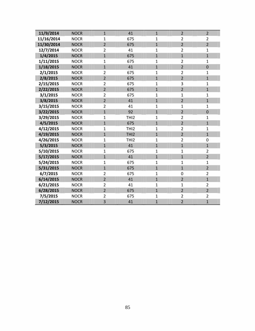
85
11/9/2014 NOCR 1 41 1 2 2 11/16/2014 NOCR 1 675 1 2 2 11/30/2014 NOCR 2 675 1 2 2 12/7/2014 NOCR 2 41 1 2 1 1/4/2015 NOCR 1 675 1 1 1
1/11/2015 NOCR 1 675 1 2 1 1/18/2015 NOCR 1 41 1 2 0 2/1/2015 NOCR 2 675 1 2 1 2/8/2015 NOCR 2 675 1 2 1
2/15/2015 NOCR 2 675 1 3 1 2/22/2015 NOCR 2 675 1 2 1 3/1/2015 NOCR 2 675 1 1 1 3/8/2015 NOCR 2 41 1 2 1
3/15/2015 NOCR 2 41 1 1 1 3/22/2015 NOCR 1 92 1 2 0 3/29/2015 NOCR 1 THI2 1 2 1 4/5/2015 NOCR 1 675 1 2 1
4/12/2015 NOCR 1 THI2 1 2 1 4/19/2015 NOCR 1 THI2 1 2 1 4/26/2015 NOCR 1 THI2 1 2 0 5/3/2015 NOCR 1 41 1 1 1
5/10/2015 NOCR 1 675 1 1 2 5/17/2015 NOCR 1 41 1 1 2 5/24/2015 NOCR 1 675 1 1 1 5/31/2015 NOCR 1 675 1 1 2 6/7/2015 NOCR 2 675 1 0 2
6/14/2015 NOCR 2 41 1 2 1 6/21/2015 NOCR 2 41 1 1 2 6/28/2015 NOCR 2 675 1 2 2 7/5/2015 NOCR 2 675 1 2 2
7/12/2015 NOCR 3 41 1 2 1
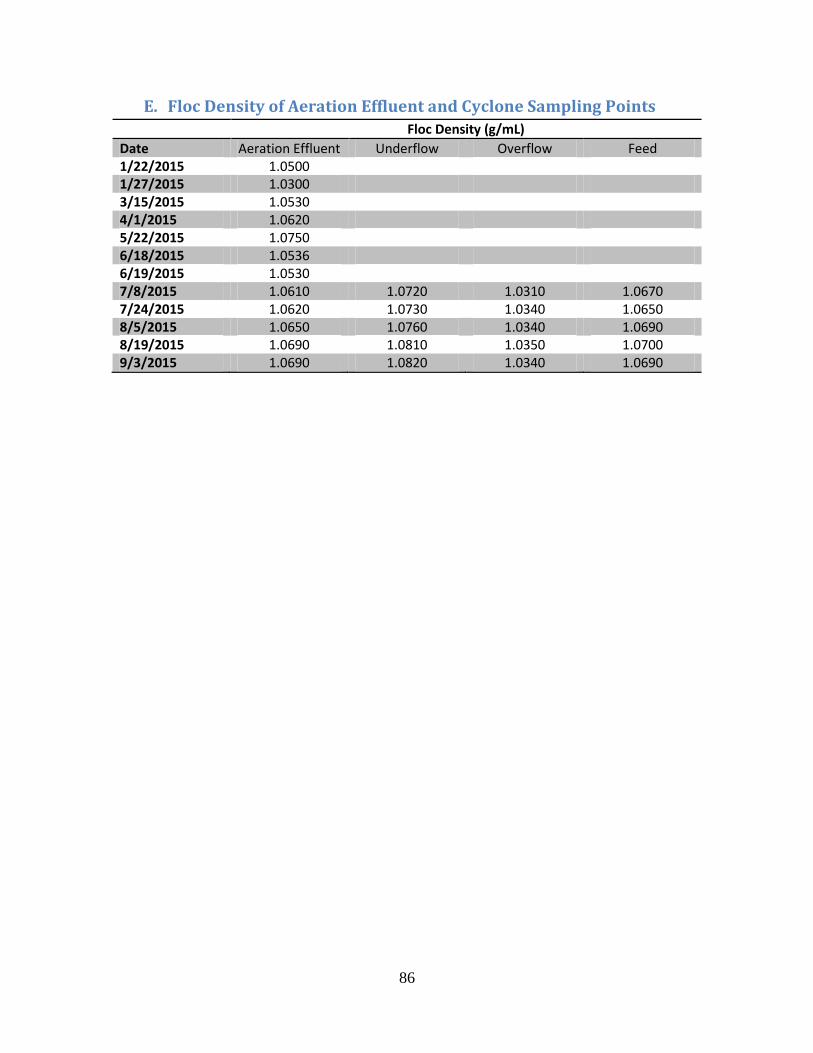
86
E. Floc Density of Aeration Effluent and Cyclone Sampling Points
Floc Density (g/mL)
Date Aeration Effluent Underflow Overflow Feed 1/22/2015 1.0500 1/27/2015 1.0300 3/15/2015 1.0530 4/1/2015 1.0620 5/22/2015 1.0750 6/18/2015 1.0536 6/19/2015 1.0530 7/8/2015 1.0610 1.0720 1.0310 1.0670 7/24/2015 1.0620 1.0730 1.0340 1.0650 8/5/2015 1.0650 1.0760 1.0340 1.0690 8/19/2015 1.0690 1.0810 1.0350 1.0700 9/3/2015 1.0690 1.0820 1.0340 1.0690
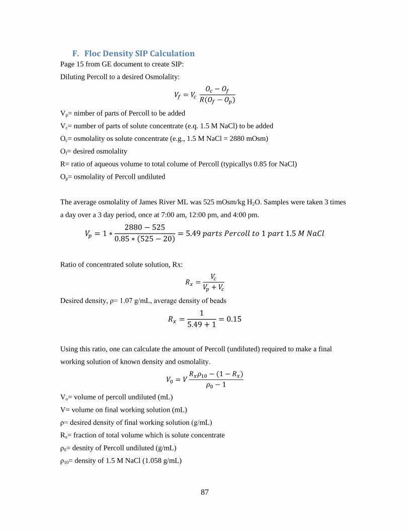
87
F. Floc Density SIP Calculation Page 15 from GE document to create SIP:
Diluting Percoll to a desired Osmolality:
Vp= nimber of parts of Percoll to be added
Vc= number of parts of solute concentrate (e.q. 1.5 M NaCl) to be added
Oc= osmolality os solute concentrate (e.g., 1.5 M NaCl = 2880 mOsm)
Of= desired osmolality
R= ratio of aqueous volume to total colume of Percoll (typicallys 0.85 for NaCl)
Op= osmolality of Percoll undiluted
The average osmolality of James River ML was 525 mOsm/kg H2O. Samples were taken 3 times
a day over a 3 day period, once at 7:00 am, 12:00 pm, and 4:00 pm.
Ratio of concentrated solute solution, Rx:
Desired density, ρ= 1.07 g/mL, average density of beads
Using this ratio, one can calculate the amount of Percoll (undiluted) required to make a final
working solution of known density and osmolality.
Vo= volume of percoll undiluted (mL)
V= volume on final working solution (mL)
ρ= desired density of final working solution (g/mL)
Rx= fraction of total volume which is solute concentrate
ρ0= desnity of Percoll undiluted (g/mL)
ρ10= density of 1.5 M NaCl (1.058 g/mL)
88
(
) (
)
( )
Final Working SIP:
47.15 mL Percoll
37.85 mL Distilled Water
15 mL 1.5 M NaCl
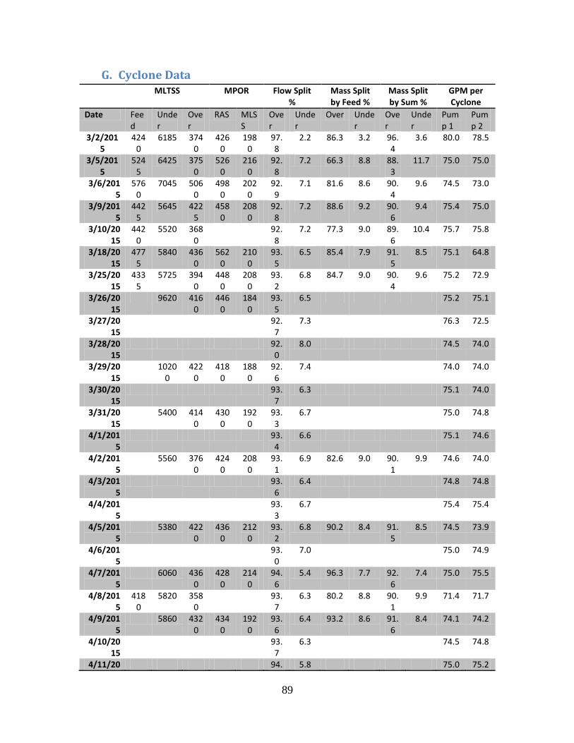
89
G. Cyclone Data MLTSS MPOR Flow Split
% Mass Split by Feed %
Mass Split by Sum %
GPM per Cyclone
Date Feed
Under
Over
RAS MLSS
Over
Under
Over Under
Over
Under
Pump 1
Pump 2
3/2/2015
4240
6185 3740
4260
1980
97.8
2.2 86.3 3.2 96.4
3.6 80.0 78.5
3/5/2015
5245
6425 3750
5260
2160
92.8
7.2 66.3 8.8 88.3
11.7 75.0 75.0
3/6/2015
5760
7045 5060
4980
2020
92.9
7.1 81.6 8.6 90.4
9.6 74.5 73.0
3/9/2015
4425
5645 4225
4580
2080
92.8
7.2 88.6 9.2 90.6
9.4 75.4 75.0
3/10/2015
4420
5520 3680
92.8
7.2 77.3 9.0 89.6
10.4 75.7 75.8
3/18/2015
4775
5840 4360
5620
2100
93.5
6.5 85.4 7.9 91.5
8.5 75.1 64.8
3/25/2015
4335
5725 3940
4480
2080
93.2
6.8 84.7 9.0 90.4
9.6 75.2 72.9
3/26/2015
9620 4160
4460
1840
93.5
6.5 75.2 75.1
3/27/2015
92.7
7.3 76.3 72.5
3/28/2015
92.0
8.0 74.5 74.0
3/29/2015
10200
4220
4180
1880
92.6
7.4 74.0 74.0
3/30/2015
93.7
6.3 75.1 74.0
3/31/2015
5400 4140
4300
1920
93.3
6.7 75.0 74.8
4/1/2015
93.4
6.6 75.1 74.6
4/2/2015
5560 3760
4240
2080
93.1
6.9 82.6 9.0 90.1
9.9 74.6 74.0
4/3/2015
93.6
6.4 74.8 74.8
4/4/2015
93.3
6.7 75.4 75.4
4/5/2015
5380 4220
4360
2120
93.2
6.8 90.2 8.4 91.5
8.5 74.5 73.9
4/6/2015
93.0
7.0 75.0 74.9
4/7/2015
6060 4360
4280
2140
94.6
5.4 96.3 7.7 92.6
7.4 75.0 75.5
4/8/2015
4180
5820 3580
93.7
6.3 80.2 8.8 90.1
9.9 71.4 71.7
4/9/2015
5860 4320
4340
1920
93.6
6.4 93.2 8.6 91.6
8.4 74.1 74.2
4/10/2015
93.7
6.3 74.5 74.8
4/11/20 94. 5.8 75.0 75.2
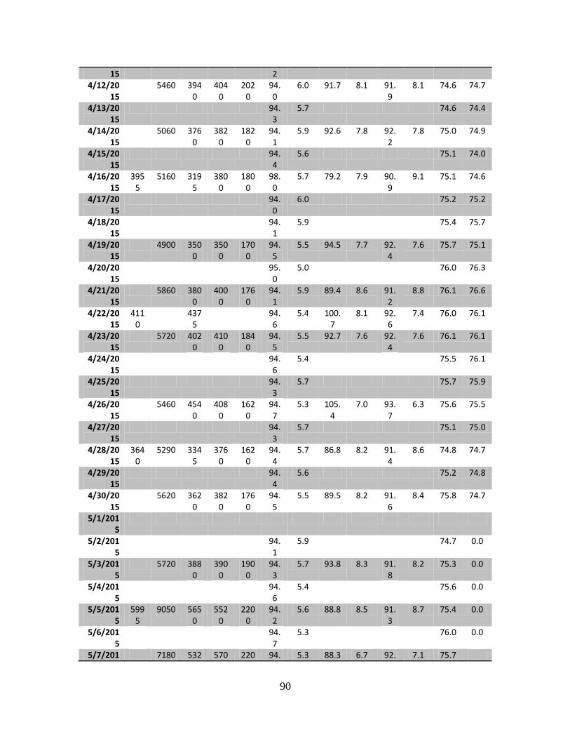
90
15 2 4/12/20
15 5460 394
0 404
0 202
0 94.0
6.0 91.7 8.1 91.9
8.1 74.6 74.7
4/13/2015
94.3
5.7 74.6 74.4
4/14/2015
5060 3760
3820
1820
94.1
5.9 92.6 7.8 92.2
7.8 75.0 74.9
4/15/2015
94.4
5.6 75.1 74.0
4/16/2015
3955
5160 3195
3800
1800
98.0
5.7 79.2 7.9 90.9
9.1 75.1 74.6
4/17/2015
94.0
6.0 75.2 75.2
4/18/2015
94.1
5.9 75.4 75.7
4/19/2015
4900 3500
3500
1700
94.5
5.5 94.5 7.7 92.4
7.6 75.7 75.1
4/20/2015
95.0
5.0 76.0 76.3
4/21/2015
5860 3800
4000
1760
94.1
5.9 89.4 8.6 91.2
8.8 76.1 76.6
4/22/2015
4110
4375
94.6
5.4 100.7
8.1 92.6
7.4 76.0 76.1
4/23/2015
5720 4020
4100
1840
94.5
5.5 92.7 7.6 92.4
7.6 76.1 76.1
4/24/2015
94.6
5.4 75.5 76.1
4/25/2015
94.3
5.7 75.7 75.9
4/26/2015
5460 4540
4080
1620
94.7
5.3 105.4
7.0 93.7
6.3 75.6 75.5
4/27/2015
94.3
5.7 75.1 75.0
4/28/2015
3640
5290 3345
3760
1620
94.4
5.7 86.8 8.2 91.4
8.6 74.8 74.7
4/29/2015
94.4
5.6 75.2 74.8
4/30/2015
5620 3620
3820
1760
94.5
5.5 89.5 8.2 91.6
8.4 75.8 74.7
5/1/2015
5/2/2015
94.1
5.9 74.7 0.0
5/3/2015
5720 3880
3900
1900
94.3
5.7 93.8 8.3 91.8
8.2 75.3 0.0
5/4/2015
94.6
5.4 75.6 0.0
5/5/2015
5995
9050 5650
5520
2200
94.2
5.6 88.8 8.5 91.3
8.7 75.4 0.0
5/6/2015
94.7
5.3 76.0 0.0
5/7/201 7180 532 570 220 94. 5.3 88.3 6.7 92. 7.1 75.7
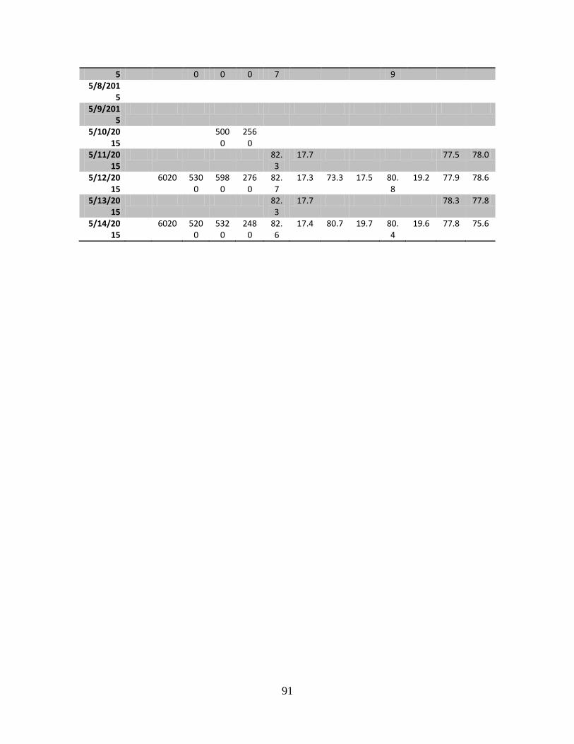
91
5 0 0 0 7 9 5/8/201
5
5/9/2015
5/10/2015
5000
2560
5/11/2015
82.3
17.7 77.5 78.0
5/12/2015
6020 5300
5980
2760
82.7
17.3 73.3 17.5 80.8
19.2 77.9 78.6
5/13/2015
82.3
17.7 78.3 77.8
5/14/2015
6020 5200
5320
2480
82.6
17.4 80.7 19.7 80.4
19.6 77.8 75.6
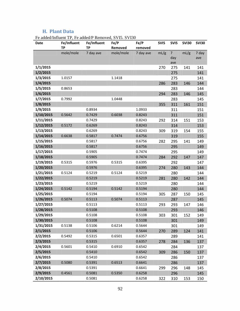
92
H. Plant Data Fe added/Influent TP, Fe added/P Removed, SVI5. SVI30
Date Fe/Influent TP
Fe/Influent TP
Fe/P Removed
Fe/P removed
SVI5 SVI5 SVI30 SVI30
mole/mole 7 day ave mole/mole 7 day ave mL/g 7 day ave
mL/g 7 day ave
1/1/2015 270 275 141 141 1/2/2015 275 141 1/3/2015 1.0157 1.1418 275 141 1/4/2015 286 283 146 144 1/5/2015 0.8653 283 144 1/6/2015 294 283 146 145 1/7/2015 0.7992 1.0448 283 145 1/8/2015 355 311 161 151 1/9/2015 0.8934 1.0933 311 151 1/10/2015 0.5642 0.7429 0.6038 0.8243 311 151 1/11/2015 0.7429 0.8243 292 314 151 153 1/12/2015 0.5172 0.6269 0.8243 314 153 1/13/2015 0.6269 0.8243 309 319 154 155 1/14/2015 0.6638 0.5817 0.7474 0.6756 319 155 1/15/2015 0.5817 0.6756 282 295 141 149 1/16/2015 0.5817 0.6756 295 149 1/17/2015 0.5905 0.7474 295 149 1/18/2015 0.5905 0.7474 284 292 147 147 1/19/2015 0.5315 0.5976 0.5315 0.6395 292 147 1/20/2015 0.5976 0.6395 274 280 143 144 1/21/2015 0.5124 0.5219 0.5124 0.5219 280 144 1/22/2015 0.5219 0.5219 281 280 142 144 1/23/2015 0.5219 0.5219 280 144 1/24/2015 0.5142 0.5194 0.5142 0.5194 280 144 1/25/2015 0.5194 0.5194 305 287 150 145 1/26/2015 0.5074 0.5113 0.5074 0.5113 287 145 1/27/2015 0.5113 0.5113 293 293 147 146 1/28/2015 0.5108 0.5108 293 146 1/29/2015 0.5108 0.5108 303 301 152 149 1/30/2015 0.5108 0.5108 301 149 1/31/2015 0.5138 0.5106 0.6214 0.5644 301 149 2/1/2015 0.5106 0.5644 270 289 124 141 2/2/2015 0.5492 0.5315 0.6501 0.6357 289 141 2/3/2015 0.5315 0.6357 278 284 136 137 2/4/2015 0.5601 0.5410 0.6910 0.6542 284 137 2/5/2015 0.5410 0.6542 309 286 150 137 2/6/2015 0.5410 0.6542 286 137 2/7/2015 0.5080 0.5391 0.6513 0.6641 286 137 2/8/2015 0.5391 0.6641 299 296 148 145 2/9/2015 0.4561 0.5081 0.5350 0.6258 296 145 2/10/2015 0.5081 0.6258 322 310 153 150
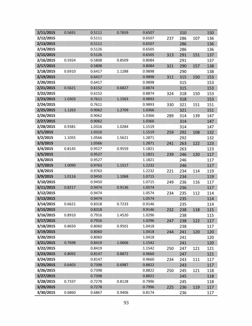
93
2/11/2015 0.5691 0.5111 0.7659 0.6507 310 150 2/12/2015 0.5111 0.6507 237 286 107 136 2/13/2015 0.5111 0.6507 286 136 2/14/2015 0.5126 0.6505 286 136 2/15/2015 0.5126 0.6505 313 291 151 137 2/16/2015 0.5924 0.5808 0.8509 0.8084 291 137 2/17/2015 0.5808 0.8084 321 290 157 138 2/18/2015 0.6910 0.6417 1.1288 0.9898 290 138 2/19/2015 0.6417 0.9898 311 315 150 153 2/20/2015 0.6417 0.9898 315 153 2/21/2015 0.5621 0.6152 0.6827 0.8874 315 153 2/22/2015 0.6152 0.8874 324 318 150 153 2/23/2015 1.0303 0.7611 1.1563 0.9893 318 153 2/24/2015 0.7611 0.9893 330 321 151 151 2/25/2015 1.1263 0.9062 1.2709 1.0366 321 151 2/26/2015 0.9062 1.0366 289 314 139 147 2/27/2015 0.9062 1.0366 314 147 2/28/2015 0.9381 1.0316 1.0284 1.1519 314 147 3/1/2015 1.0316 1.1519 259 292 108 132 3/2/2015 1.1055 1.0566 1.5621 1.2871 292 132 3/3/2015 1.0566 1.2871 241 263 122 123 3/4/2015 0.8145 0.9527 0.9559 1.1821 263 123 3/5/2015 0.9527 1.1821 239 246 120 117 3/6/2015 0.9527 1.1821 246 117 3/7/2015 1.0090 0.9763 1.1517 1.2232 246 117 3/8/2015 0.9763 1.2232 221 234 114 119 3/9/2015 1.0116 0.9450 1.1068 1.0715 234 119 3/10/2015 0.9450 1.0715 249 236 116 117 3/11/2015 0.8217 0.9474 0.9136 1.0574 236 117 3/12/2015 0.9474 1.0574 234 235 112 114 3/13/2015 0.9474 1.0574 235 114 3/14/2015 0.6621 0.8318 0.7233 0.9146 235 114 3/15/2015 0.8318 0.9146 232 238 118 115 3/16/2015 0.8910 0.7916 1.4520 1.0296 238 115 3/17/2015 0.7916 1.0296 247 238 122 117 3/18/2015 0.8650 0.8060 0.9501 1.0418 238 117 3/19/2015 0.8060 1.0418 244 241 120 120 3/20/2015 0.8060 1.0418 241 120 3/21/2015 0.7698 0.8419 1.0606 1.1542 241 120 3/22/2015 0.8419 1.1542 250 247 121 121 3/23/2015 0.8092 0.8147 0.8872 0.9660 247 121 3/24/2015 0.8147 0.9660 234 243 111 117 3/25/2015 0.6403 0.7398 0.6987 0.8822 243 117 3/26/2015 0.7398 0.8822 250 245 121 118 3/27/2015 0.7398 0.8822 245 118 3/28/2015 0.7337 0.7278 0.8128 0.7996 245 118 3/29/2015 0.7278 0.7996 225 236 119 117 3/30/2015 0.6860 0.6867 0.9406 0.8174 236 117

94
3/31/2015 0.6867 0.8174 245 240 137 126 4/1/2015 0.7936 0.7378 0.9540 0.9025 240 126 4/2/2015 0.7378 0.9025 237 236 119 125 4/3/2015 0.7378 0.9025 236 125 4/4/2015 0.7910 0.7569 0.9500 0.9482 236 125 4/5/2015 0.7569 0.9482 258 247 126 127 4/6/2015 0.7760 0.7869 0.8597 0.9212 247 127 4/7/2015 0.7869 0.9212 260 252 132 126 4/8/2015 0.6961 0.7544 0.8305 0.8801 252 126 4/9/2015 0.7544 0.8801 276 265 138 132 4/10/2015 0.7544 0.8801 265 132 4/11/2015 0.7342 0.7354 0.8295 0.8399 265 132 4/12/2015 0.7354 0.8399 241 259 124 131 4/13/2015 0.7313 0.7206 0.7985 0.8195 259 131 4/14/2015 0.7206 0.8195 253 257 132 131 4/15/2015 0.7576 0.7410 0.8626 0.8302 257 131 4/16/2015 0.7410 0.8302 254 249 132 129 4/17/2015 0.7410 0.8302 249 129 4/18/2015 0.7291 0.7393 0.8796 0.8469 249 129 4/19/2015 0.7393 0.8469 237 248 128 130 4/20/2015 0.6470 0.7112 0.7432 0.8285 248 130 4/21/2015 0.7112 0.8285 244 245 132 131 4/22/2015 0.7373 0.7045 0.8027 0.8085 245 131 4/23/2015 0.7045 0.8085 243 241 130 130 4/24/2015 0.7045 0.8085 241 130 4/25/2015 0.6515 0.6786 0.7379 0.7613 241 130 4/26/2015 0.6786 0.7613 259 249 134 132 4/27/2015 0.7610 0.7166 0.8328 0.7911 249 132 4/28/2015 0.7166 0.7911 288 263 148 138 4/29/2015 0.7708 0.7277 0.8392 0.8033 263 138 4/30/2015 0.7277 0.8033 257 268 140 141 5/1/2015 0.7277 0.8033 268 141 5/2/2015 0.6853 0.7390 0.7584 0.8101 268 141 5/3/2015 0.7390 0.8101 242 263 128 139 5/4/2015 0.6627 0.7062 0.7142 0.7706 263 139 5/5/2015 0.7062 0.7706 245 248 132 133 5/6/2015 0.7048 0.6842 0.7426 0.7384 248 133 5/7/2015 0.6842 0.7384 232 240 132 131 5/8/2015 0.6842 0.7384 240 131 5/9/2015 0.6538 0.6737 0.7809 0.7459 240 131 5/10/2015 0.6737 0.7459 275 251 145 136 5/11/2015 0.6874 0.6820 0.7229 0.7488 251 136 5/12/2015 0.6820 0.7488 278 261 149 142 5/13/2015 0.6103 0.6505 0.6397 0.7145 261 142 5/14/2015 0.6505 0.7145 313 289 164 152 5/15/2015 0.6505 0.7145 289 152 5/16/2015 0.5786 0.6254 0.6445 0.6690 289 152 5/17/2015 0.6254 0.6690 263 285 141 151

95
5/18/2015 0.5056 0.5648 0.5959 0.6267 285 151 5/19/2015 0.5648 0.6267 269 282 148 151 5/20/2015 0.4010 0.4951 0.4241 0.5548 282 151 5/21/2015 0.4951 0.5548 253 262 141 143 5/22/2015 0.4951 0.5548 262 143 5/23/2015 0.4533 0.5100 262 143 5/24/2015 0.4533 0.5100 245 256 133 141 5/25/2015 0.4112 0.4061 0.4241 256 141 5/26/2015 0.4061 0.4241 223 241 133 135 5/27/2015 0.3972 0.4042 0.4241 241 135 5/28/2015 0.4042 0.4241 233 234 130 132 5/29/2015 0.4042 0.2955 234 132 5/30/2015 0.2810 0.3631 0.2955 0.2955 234 132 5/31/2015 0.3631 0.2955 207 221 123 128 6/1/2015 0.2068 0.2950 0.2916 0.2935 221 128 6/2/2015 0.2950 0.2935 221 220 121 125 6/3/2015 0.2588 0.2489 0.3183 0.3018 220 125 6/4/2015 0.2489 0.3018 204 210 120 121 6/5/2015 0.2489 0.3018 210 121 6/6/2015 0.3143 0.2600 0.3467 0.3189 210 121 6/7/2015 0.2600 0.3189 242 222 136 126 6/8/2015 0.1978 0.2570 0.2459 0.3037 222 126 6/9/2015 0.2570 0.3037 250 232 143 133 6/10/2015 0.2201 0.2441 0.2398 0.2775 232 133 6/11/2015 0.2441 0.2775 225 239 131 137 6/12/2015 0.2441 0.2775 239 137 6/13/2015 0.2298 0.2159 0.2935 0.2597 239 137 6/14/2015 0.2159 0.2597 216 231 132 135 6/15/2015 0.2304 0.2268 0.2645 0.2659 231 135 6/16/2015 0.2268 0.2659 234 225 139 134 6/17/2015 0.3278 0.2627 0.4046 0.3209 225 134 6/18/2015 0.2627 0.3209 269 240 146 139 6/19/2015 0.2627 0.3209 240 139 6/20/2015 0.3225 0.2936 0.3955 0.3549 240 139 6/21/2015 0.2936 0.3549 232 245 135 140 6/22/2015 0.3397 0.3300 0.7448 0.5150 245 140 6/23/2015 0.3300 0.5150 264 255 154 145 6/24/2015 0.4681 0.3768 0.5378 0.5594 255 145 6/25/2015 0.3768 0.5594 257 251 147 145 6/26/2015 0.3768 0.5594 251 145 6/27/2015 0.8607 0.5562 1.5204 0.9343 251 145 6/28/2015 0.5562 0.9343 291 271 165 155 6/29/2015 0.6977 0.6755 0.7499 0.9360 271 155 6/30/2015 0.6755 0.9360 247 265 142 151 7/1/2015 0.6529 0.7371 0.7566 1.0090 265 151 7/2/2015 0.7371 1.0090 242 260 140 149 7/3/2015 0.7371 1.0090 260 149 7/4/2015 0.7326 0.6944 0.7822 0.7629 260 149
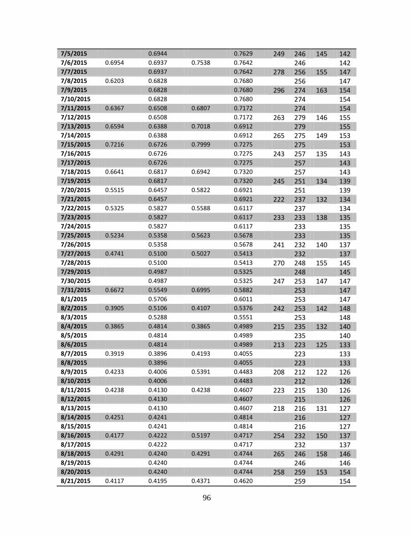
96
7/5/2015 0.6944 0.7629 249 246 145 142 7/6/2015 0.6954 0.6937 0.7538 0.7642 246 142 7/7/2015 0.6937 0.7642 278 256 155 147 7/8/2015 0.6203 0.6828 0.7680 256 147 7/9/2015 0.6828 0.7680 296 274 163 154 7/10/2015 0.6828 0.7680 274 154 7/11/2015 0.6367 0.6508 0.6807 0.7172 274 154 7/12/2015 0.6508 0.7172 263 279 146 155 7/13/2015 0.6594 0.6388 0.7018 0.6912 279 155 7/14/2015 0.6388 0.6912 265 275 149 153 7/15/2015 0.7216 0.6726 0.7999 0.7275 275 153 7/16/2015 0.6726 0.7275 243 257 135 143 7/17/2015 0.6726 0.7275 257 143 7/18/2015 0.6641 0.6817 0.6942 0.7320 257 143 7/19/2015 0.6817 0.7320 245 251 134 139 7/20/2015 0.5515 0.6457 0.5822 0.6921 251 139 7/21/2015 0.6457 0.6921 222 237 132 134 7/22/2015 0.5325 0.5827 0.5588 0.6117 237 134 7/23/2015 0.5827 0.6117 233 233 138 135 7/24/2015 0.5827 0.6117 233 135 7/25/2015 0.5234 0.5358 0.5623 0.5678 233 135 7/26/2015 0.5358 0.5678 241 232 140 137 7/27/2015 0.4741 0.5100 0.5027 0.5413 232 137 7/28/2015 0.5100 0.5413 270 248 155 145 7/29/2015 0.4987 0.5325 248 145 7/30/2015 0.4987 0.5325 247 253 147 147 7/31/2015 0.6672 0.5549 0.6995 0.5882 253 147 8/1/2015 0.5706 0.6011 253 147 8/2/2015 0.3905 0.5106 0.4107 0.5376 242 253 142 148 8/3/2015 0.5288 0.5551 253 148 8/4/2015 0.3865 0.4814 0.3865 0.4989 215 235 132 140 8/5/2015 0.4814 0.4989 235 140 8/6/2015 0.4814 0.4989 213 223 125 133 8/7/2015 0.3919 0.3896 0.4193 0.4055 223 133 8/8/2015 0.3896 0.4055 223 133 8/9/2015 0.4233 0.4006 0.5391 0.4483 208 212 122 126 8/10/2015 0.4006 0.4483 212 126 8/11/2015 0.4238 0.4130 0.4238 0.4607 223 215 130 126 8/12/2015 0.4130 0.4607 215 126 8/13/2015 0.4130 0.4607 218 216 131 127 8/14/2015 0.4251 0.4241 0.4814 216 127 8/15/2015 0.4241 0.4814 216 127 8/16/2015 0.4177 0.4222 0.5197 0.4717 254 232 150 137 8/17/2015 0.4222 0.4717 232 137 8/18/2015 0.4291 0.4240 0.4291 0.4744 265 246 158 146 8/19/2015 0.4240 0.4744 246 146 8/20/2015 0.4240 0.4744 258 259 153 154 8/21/2015 0.4117 0.4195 0.4371 0.4620 259 154
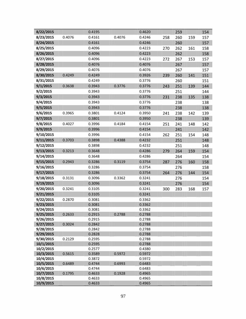
97
8/22/2015 0.4195 0.4620 259 154 8/23/2015 0.4076 0.4161 0.4076 0.4246 258 260 159 157 8/24/2015 0.4161 0.4246 260 157 8/25/2015 0.4096 0.4223 270 262 161 158 8/26/2015 0.4096 0.4223 262 158 8/27/2015 0.4096 0.4223 272 267 153 157 8/28/2015 0.4076 0.4076 267 157 8/29/2015 0.4076 0.4076 267 157 8/30/2015 0.4249 0.4249 0.3926 239 260 141 151 8/31/2015 0.4249 0.3776 260 151 9/1/2015 0.3638 0.3943 0.3776 0.3776 243 251 139 144 9/2/2015 0.3943 0.3776 251 144 9/3/2015 0.3943 0.3776 231 238 135 138 9/4/2015 0.3943 0.3776 238 138 9/5/2015 0.3943 0.3776 238 138 9/6/2015 0.3965 0.3801 0.4124 0.3950 241 238 142 139 9/7/2015 0.3801 0.3950 238 139 9/8/2015 0.4027 0.3996 0.4184 0.4154 251 241 148 142 9/9/2015 0.3996 0.4154 241 142 9/10/2015 0.3996 0.4154 262 251 154 148 9/11/2015 0.3703 0.3898 0.4388 0.4232 251 148 9/12/2015 0.3898 0.4232 251 148 9/13/2015 0.3213 0.3648 0.4286 279 264 159 154 9/14/2015 0.3648 0.4286 264 154 9/15/2015 0.2943 0.3286 0.3119 0.3754 287 276 160 158 9/16/2015 0.3286 0.3754 276 158 9/17/2015 0.3286 0.3754 264 276 144 154 9/18/2015 0.3131 0.3096 0.3362 0.3241 276 154 9/19/2015 0.3096 0.3241 276 154 9/20/2015 0.3241 0.3105 0.3241 300 283 168 157 9/21/2015 0.3105 0.3241 9/22/2015 0.2870 0.3081 0.3362 9/23/2015 0.3081 0.3362 9/24/2015 0.3081 0.3362 9/25/2015 0.2633 0.2915 0.2788 0.2788 9/26/2015 0.2915 0.2788 9/27/2015 0.3024 0.2842 0.2788 9/28/2015 0.2842 0.2788 9/29/2015 0.2828 0.2788 9/30/2015 0.2129 0.2595 0.2788 10/1/2015 0.2595 0.2788 10/2/2015 0.2577 0.4380 10/3/2015 0.5615 0.3589 0.5972 0.5972 10/4/2015 0.3872 0.5972 10/5/2015 0.6489 0.4744 0.6993 0.6483 10/6/2015 0.4744 0.6483 10/7/2015 0.1795 0.4633 0.1928 0.4965 10/8/2015 0.4633 0.4965 10/9/2015 0.4633 0.4965

98
10/10/2015 0.4142 0.4461 10/11/2015 0.4142 0.4461 10/12/2015 0.2280 0.2037 0.1928
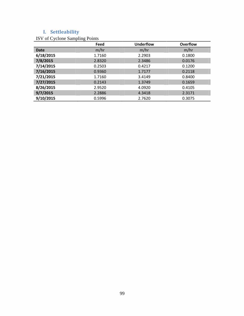
99
I. Settleability ISV of Cyclone Sampling Points
Feed Underflow Overflow
Date m/hr m/hr m/hr 6/18/2015 1.7160 2.2903 0.1800 7/8/2015 2.8320 2.3486 0.0176 7/14/2015 0.2503 0.4217 0.1200 7/16/2015 0.9360 1.7177 0.2118 7/21/2015 1.7160 3.4149 0.8400 7/27/2015 0.2143 1.3749 0.1659 8/26/2015 2.9520 4.0920 0.4105 9/7/2015 2.2886 4.3418 2.3171 9/10/2015 0.5996 2.7620 0.3075
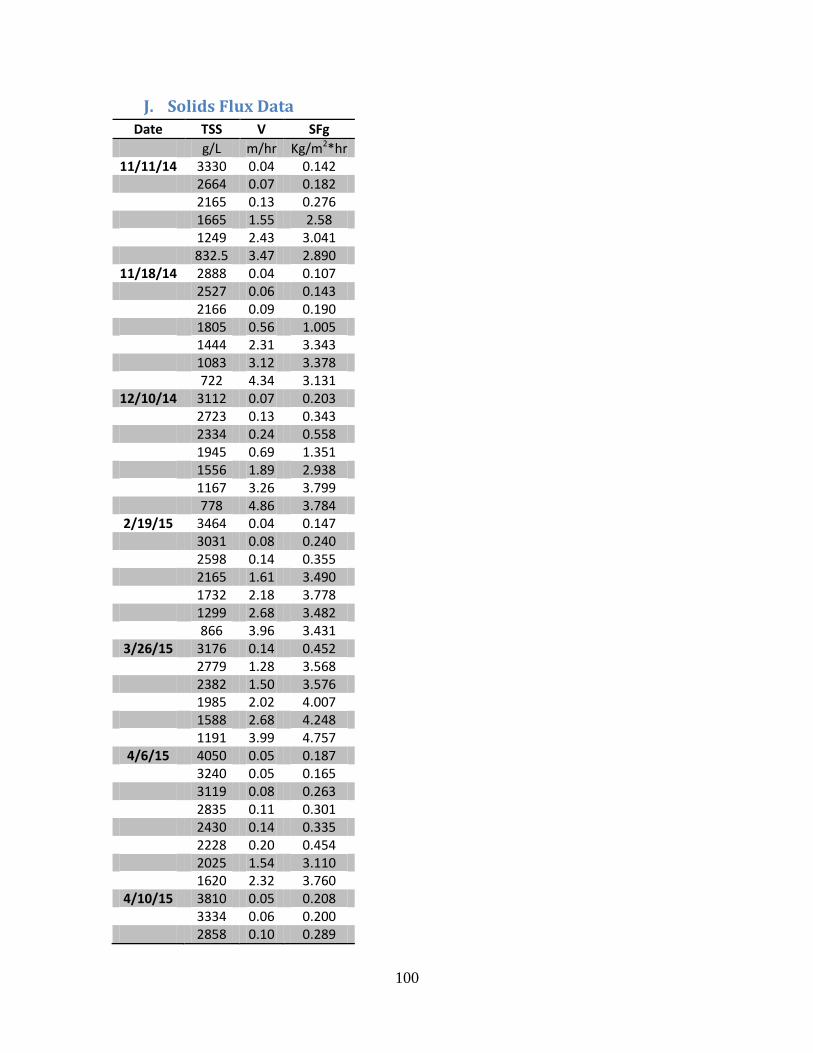
100
J. Solids Flux Data
Date TSS V SFg
g/L m/hr Kg/m2*hr 11/11/14 3330 0.04 0.142
2664 0.07 0.182 2165 0.13 0.276 1665 1.55 2.58 1249 2.43 3.041 832.5 3.47 2.890
11/18/14 2888 0.04 0.107 2527 0.06 0.143 2166 0.09 0.190 1805 0.56 1.005 1444 2.31 3.343 1083 3.12 3.378 722 4.34 3.131
12/10/14 3112 0.07 0.203 2723 0.13 0.343 2334 0.24 0.558 1945 0.69 1.351 1556 1.89 2.938 1167 3.26 3.799 778 4.86 3.784
2/19/15 3464 0.04 0.147 3031 0.08 0.240 2598 0.14 0.355 2165 1.61 3.490 1732 2.18 3.778 1299 2.68 3.482 866 3.96 3.431
3/26/15 3176 0.14 0.452 2779 1.28 3.568 2382 1.50 3.576 1985 2.02 4.007 1588 2.68 4.248 1191 3.99 4.757
4/6/15 4050 0.05 0.187 3240 0.05 0.165 3119 0.08 0.263 2835 0.11 0.301 2430 0.14 0.335 2228 0.20 0.454 2025 1.54 3.110 1620 2.32 3.760
4/10/15 3810 0.05 0.208 3334 0.06 0.200 2858 0.10 0.289
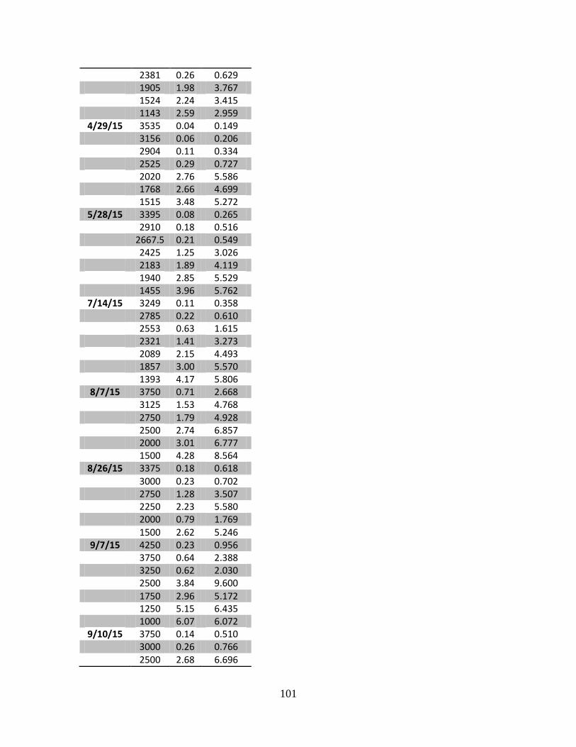
101
2381 0.26 0.629 1905 1.98 3.767 1524 2.24 3.415 1143 2.59 2.959
4/29/15 3535 0.04 0.149 3156 0.06 0.206 2904 0.11 0.334 2525 0.29 0.727 2020 2.76 5.586 1768 2.66 4.699 1515 3.48 5.272
5/28/15 3395 0.08 0.265 2910 0.18 0.516 2667.5 0.21 0.549 2425 1.25 3.026 2183 1.89 4.119 1940 2.85 5.529 1455 3.96 5.762
7/14/15 3249 0.11 0.358 2785 0.22 0.610 2553 0.63 1.615 2321 1.41 3.273 2089 2.15 4.493 1857 3.00 5.570 1393 4.17 5.806
8/7/15 3750 0.71 2.668 3125 1.53 4.768
2750 1.79 4.928 2500 2.74 6.857 2000 3.01 6.777 1500 4.28 8.564
8/26/15 3375 0.18 0.618
3000 0.23 0.702 2750 1.28 3.507 2250 2.23 5.580 2000 0.79 1.769
1500 2.62 5.246 9/7/15 4250 0.23 0.956
3750 0.64 2.388 3250 0.62 2.030 2500 3.84 9.600 1750 2.96 5.172 1250 5.15 6.435 1000 6.07 6.072
9/10/15 3750 0.14 0.510 3000 0.26 0.766 2500 2.68 6.696

102
2000 3.39 6.789 1750 5.40 9.450
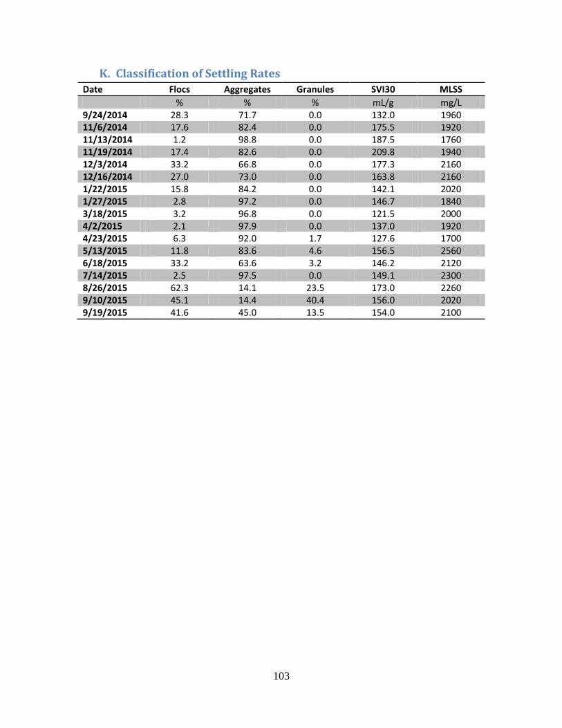
103
K. Classification of Settling Rates
Date Flocs Aggregates Granules SVI30 MLSS
% % % mL/g mg/L 9/24/2014 28.3 71.7 0.0 132.0 1960 11/6/2014 17.6 82.4 0.0 175.5 1920 11/13/2014 1.2 98.8 0.0 187.5 1760 11/19/2014 17.4 82.6 0.0 209.8 1940 12/3/2014 33.2 66.8 0.0 177.3 2160 12/16/2014 27.0 73.0 0.0 163.8 2160 1/22/2015 15.8 84.2 0.0 142.1 2020 1/27/2015 2.8 97.2 0.0 146.7 1840 3/18/2015 3.2 96.8 0.0 121.5 2000 4/2/2015 2.1 97.9 0.0 137.0 1920 4/23/2015 6.3 92.0 1.7 127.6 1700 5/13/2015 11.8 83.6 4.6 156.5 2560 6/18/2015 33.2 63.6 3.2 146.2 2120 7/14/2015 2.5 97.5 0.0 149.1 2300 8/26/2015 62.3 14.1 23.5 173.0 2260 9/10/2015 45.1 14.4 40.4 156.0 2020 9/19/2015 41.6 45.0 13.5 154.0 2100
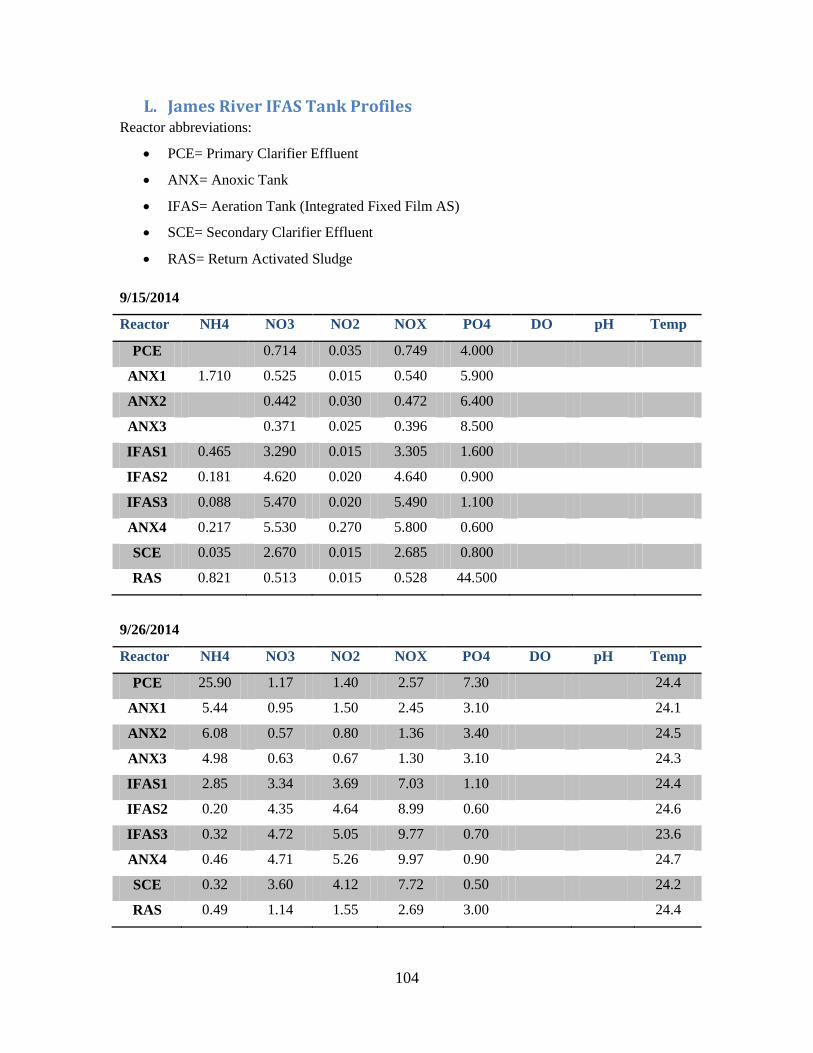
104
L. James River IFAS Tank Profiles Reactor abbreviations:
PCE= Primary Clarifier Effluent
ANX= Anoxic Tank
IFAS= Aeration Tank (Integrated Fixed Film AS)
SCE= Secondary Clarifier Effluent
RAS= Return Activated Sludge
9/15/2014
Reactor NH4 NO3 NO2 NOX PO4 DO pH Temp
PCE 0.714 0.035 0.749 4.000
ANX1 1.710 0.525 0.015 0.540 5.900
ANX2 0.442 0.030 0.472 6.400
ANX3 0.371 0.025 0.396 8.500
IFAS1 0.465 3.290 0.015 3.305 1.600
IFAS2 0.181 4.620 0.020 4.640 0.900
IFAS3 0.088 5.470 0.020 5.490 1.100
ANX4 0.217 5.530 0.270 5.800 0.600
SCE 0.035 2.670 0.015 2.685 0.800
RAS 0.821 0.513 0.015 0.528 44.500
9/26/2014
Reactor NH4 NO3 NO2 NOX PO4 DO pH Temp
PCE 25.90 1.17 1.40 2.57 7.30 24.4
ANX1 5.44 0.95 1.50 2.45 3.10 24.1
ANX2 6.08 0.57 0.80 1.36 3.40 24.5
ANX3 4.98 0.63 0.67 1.30 3.10 24.3
IFAS1 2.85 3.34 3.69 7.03 1.10 24.4
IFAS2 0.20 4.35 4.64 8.99 0.60 24.6
IFAS3 0.32 4.72 5.05 9.77 0.70 23.6
ANX4 0.46 4.71 5.26 9.97 0.90 24.7
SCE 0.32 3.60 4.12 7.72 0.50 24.2
RAS 0.49 1.14 1.55 2.69 3.00 24.4
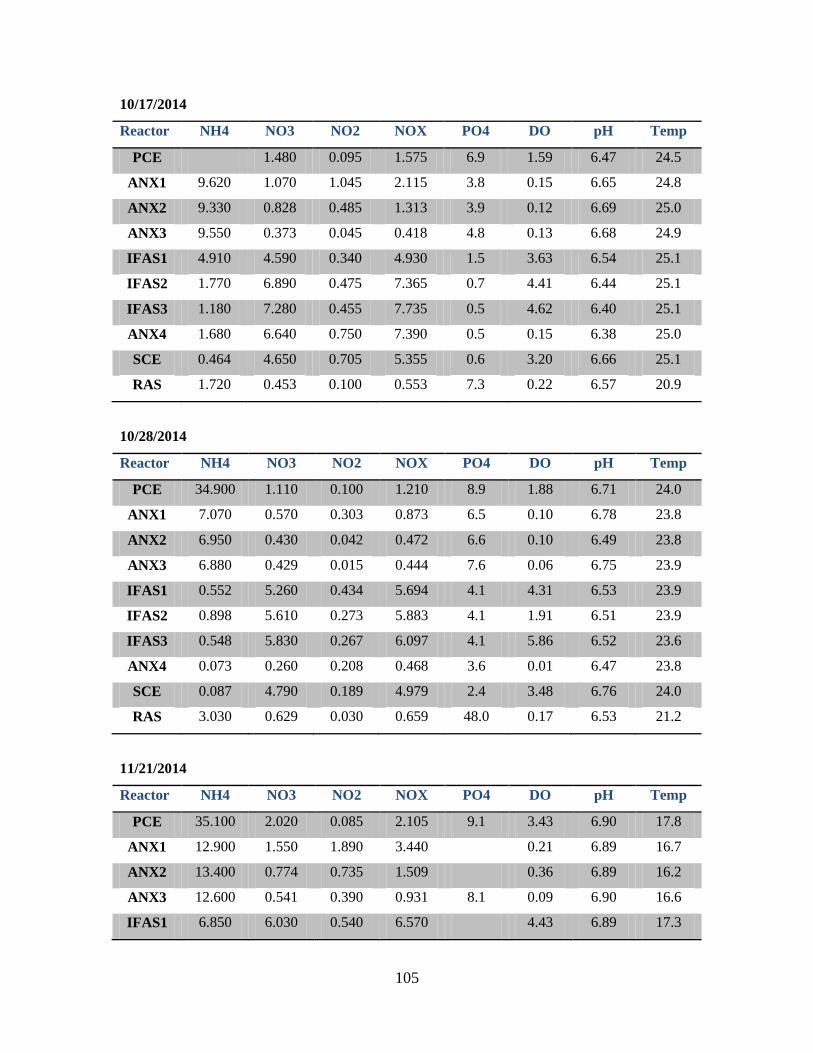
105
10/17/2014
Reactor NH4 NO3 NO2 NOX PO4 DO pH Temp
PCE 1.480 0.095 1.575 6.9 1.59 6.47 24.5
ANX1 9.620 1.070 1.045 2.115 3.8 0.15 6.65 24.8
ANX2 9.330 0.828 0.485 1.313 3.9 0.12 6.69 25.0
ANX3 9.550 0.373 0.045 0.418 4.8 0.13 6.68 24.9
IFAS1 4.910 4.590 0.340 4.930 1.5 3.63 6.54 25.1
IFAS2 1.770 6.890 0.475 7.365 0.7 4.41 6.44 25.1
IFAS3 1.180 7.280 0.455 7.735 0.5 4.62 6.40 25.1
ANX4 1.680 6.640 0.750 7.390 0.5 0.15 6.38 25.0
SCE 0.464 4.650 0.705 5.355 0.6 3.20 6.66 25.1
RAS 1.720 0.453 0.100 0.553 7.3 0.22 6.57 20.9
10/28/2014
Reactor NH4 NO3 NO2 NOX PO4 DO pH Temp
PCE 34.900 1.110 0.100 1.210 8.9 1.88 6.71 24.0
ANX1 7.070 0.570 0.303 0.873 6.5 0.10 6.78 23.8
ANX2 6.950 0.430 0.042 0.472 6.6 0.10 6.49 23.8
ANX3 6.880 0.429 0.015 0.444 7.6 0.06 6.75 23.9
IFAS1 0.552 5.260 0.434 5.694 4.1 4.31 6.53 23.9
IFAS2 0.898 5.610 0.273 5.883 4.1 1.91 6.51 23.9
IFAS3 0.548 5.830 0.267 6.097 4.1 5.86 6.52 23.6
ANX4 0.073 0.260 0.208 0.468 3.6 0.01 6.47 23.8
SCE 0.087 4.790 0.189 4.979 2.4 3.48 6.76 24.0
RAS 3.030 0.629 0.030 0.659 48.0 0.17 6.53 21.2
11/21/2014
Reactor NH4 NO3 NO2 NOX PO4 DO pH Temp
PCE 35.100 2.020 0.085 2.105 9.1 3.43 6.90 17.8
ANX1 12.900 1.550 1.890 3.440 0.21 6.89 16.7
ANX2 13.400 0.774 0.735 1.509 0.36 6.89 16.2
ANX3 12.600 0.541 0.390 0.931 8.1 0.09 6.90 16.6
IFAS1 6.850 6.030 0.540 6.570 4.43 6.89 17.3
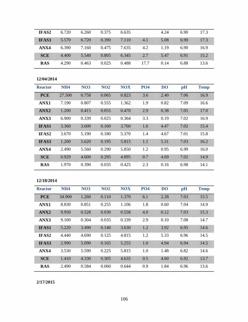
106
IFAS2 6.720 6.260 0.375 6.635 4.24 6.90 17.3
IFAS3 5.570 6.720 0.390 7.110 4.1 5.08 6.90 17.3
ANX4 6.390 7.160 0.475 7.635 4.2 1.19 6.90 16.9
SCE 4.400 5.540 0.805 6.345 2.7 5.47 6.91 15.2
RAS 4.290 0.463 0.025 0.488 17.7 0.14 6.88 13.6
12/04/2014
Reactor NH4 NO3 NO2 NOX PO4 DO pH Temp
PCE 27.500 0.758 0.065 0.823 3.6 2.40 7.06 16.9
ANX1 7.190 0.807 0.555 1.362 1.9 0.82 7.09 16.6
ANX2 1.200 0.415 0.055 0.470 2.9 0.38 7.05 17.0
ANX3 6.900 0.339 0.025 0.364 3.3 0.19 7.02 16.9
IFAS1 3.360 3.600 0.160 3.760 1.6 4.47 7.02 15.4
IFAS2 3.670 5.190 0.180 5.370 1.4 4.67 7.01 15.8
IFAS3 1.200 5.620 0.195 5.815 1.1 5.31 7.03 16.2
ANX4 2.490 5.560 0.290 5.850 1.2 0.95 6.99 16.0
SCE 0.929 4.600 0.295 4.895 0.7 4.69 7.02 14.9
RAS 1.970 0.390 0.035 0.425 2.3 0.16 6.98 14.1
12/18/2014
Reactor NH4 NO3 NO2 NOX PO4 DO pH Temp
PCE 34.900 1.260 0.110 1.370 6.1 2.28 7.03 15.5
ANX1 8.830 0.851 0.255 1.106 1.8 0.60 7.04 14.9
ANX2 9.950 0.528 0.030 0.558 4.0 0.12 7.03 15.3
ANX3 9.100 0.304 0.035 0.339 2.9 0.10 7.08 14.7
IFAS1 5.220 3.490 0.140 3.630 1.2 3.92 6.95 14.6
IFAS2 4.440 4.690 0.125 4.815 1.2 5.33 6.96 14.5
IFAS3 2.990 5.090 0.165 5.255 1.0 4.94 6.94 14.5
ANX4 3.530 5.590 0.225 5.815 1.0 1.48 6.82 14.6
SCE 1.410 4.330 0.305 4.635 0.5 4.60 6.92 13.7
RAS 2.490 0.584 0.060 0.644 0.9 1.84 6.96 13.6
2/17/2015
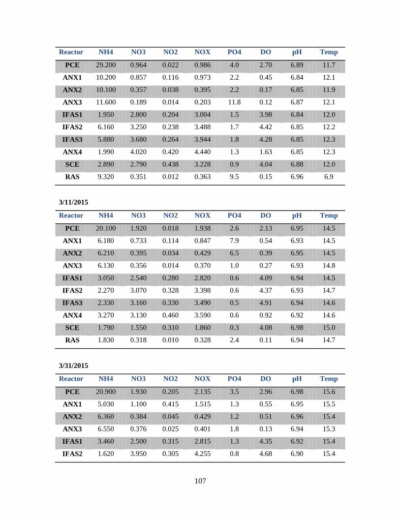
107
Reactor NH4 NO3 NO2 NOX PO4 DO pH Temp
PCE 29.200 0.964 0.022 0.986 4.0 2.70 6.89 11.7
ANX1 10.200 0.857 0.116 0.973 2.2 0.45 6.84 12.1
ANX2 10.100 0.357 0.038 0.395 2.2 0.17 6.85 11.9
ANX3 11.600 0.189 0.014 0.203 11.8 0.12 6.87 12.1
IFAS1 1.950 2.800 0.204 3.004 1.5 3.98 6.84 12.0
IFAS2 6.160 3.250 0.238 3.488 1.7 4.42 6.85 12.2
IFAS3 5.880 3.680 0.264 3.944 1.8 4.28 6.85 12.3
ANX4 1.990 4.020 0.420 4.440 1.3 1.63 6.85 12.3
SCE 2.890 2.790 0.438 3.228 0.9 4.04 6.88 12.0
RAS 9.320 0.351 0.012 0.363 9.5 0.15 6.96 6.9
3/11/2015
Reactor NH4 NO3 NO2 NOX PO4 DO pH Temp
PCE 20.100 1.920 0.018 1.938 2.6 2.13 6.95 14.5
ANX1 6.180 0.733 0.114 0.847 7.9 0.54 6.93 14.5
ANX2 6.210 0.395 0.034 0.429 6.5 0.39 6.95 14.5
ANX3 6.130 0.356 0.014 0.370 1.0 0.27 6.93 14.8
IFAS1 3.050 2.540 0.280 2.820 0.6 4.09 6.94 14.5
IFAS2 2.270 3.070 0.328 3.398 0.6 4.37 6.93 14.7
IFAS3 2.330 3.160 0.330 3.490 0.5 4.91 6.94 14.6
ANX4 3.270 3.130 0.460 3.590 0.6 0.92 6.92 14.6
SCE 1.790 1.550 0.310 1.860 0.3 4.08 6.98 15.0
RAS 1.830 0.318 0.010 0.328 2.4 0.11 6.94 14.7
3/31/2015
Reactor NH4 NO3 NO2 NOX PO4 DO pH Temp
PCE 20.900 1.930 0.205 2.135 3.5 2.96 6.98 15.6
ANX1 5.030 1.100 0.415 1.515 1.3 0.55 6.95 15.5
ANX2 6.360 0.384 0.045 0.429 1.2 0.51 6.96 15.4
ANX3 6.550 0.376 0.025 0.401 1.8 0.13 6.94 15.3
IFAS1 3.460 2.500 0.315 2.815 1.3 4.35 6.92 15.4
IFAS2 1.620 3.950 0.305 4.255 0.8 4.68 6.90 15.4
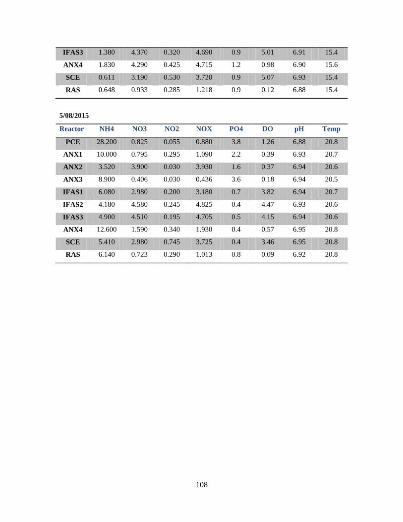
108
IFAS3 1.380 4.370 0.320 4.690 0.9 5.01 6.91 15.4
ANX4 1.830 4.290 0.425 4.715 1.2 0.98 6.90 15.6
SCE 0.611 3.190 0.530 3.720 0.9 5.07 6.93 15.4
RAS 0.648 0.933 0.285 1.218 0.9 0.12 6.88 15.4
5/08/2015
Reactor NH4 NO3 NO2 NOX PO4 DO pH Temp
PCE 28.200 0.825 0.055 0.880 3.8 1.26 6.88 20.8
ANX1 10.000 0.795 0.295 1.090 2.2 0.39 6.93 20.7
ANX2 3.520 3.900 0.030 3.930 1.6 0.37 6.94 20.6
ANX3 8.900 0.406 0.030 0.436 3.6 0.18 6.94 20.5
IFAS1 6.080 2.980 0.200 3.180 0.7 3.82 6.94 20.7
IFAS2 4.180 4.580 0.245 4.825 0.4 4.47 6.93 20.6
IFAS3 4.900 4.510 0.195 4.705 0.5 4.15 6.94 20.6
ANX4 12.600 1.590 0.340 1.930 0.4 0.57 6.95 20.8
SCE 5.410 2.980 0.745 3.725 0.4 3.46 6.95 20.8
RAS 6.140 0.723 0.290 1.013 0.8 0.09 6.92 20.8
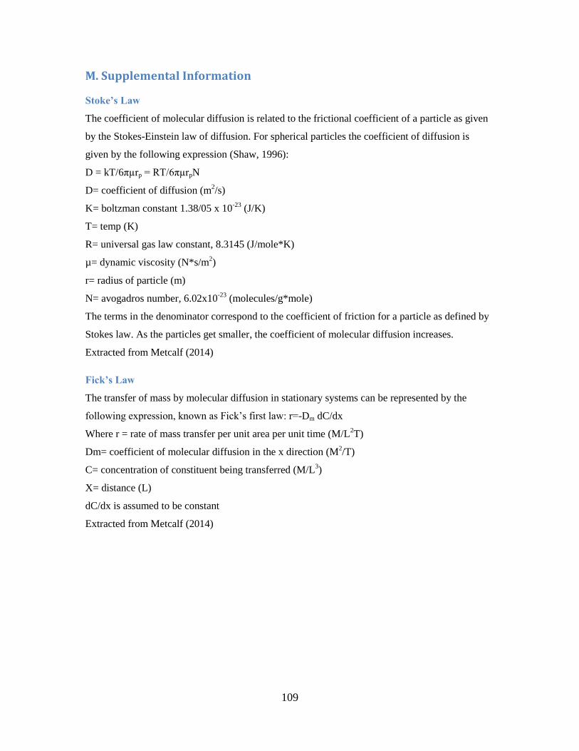
109
M. Supplemental Information
Stoke’s Law
The coefficient of molecular diffusion is related to the frictional coefficient of a particle as given
by the Stokes-Einstein law of diffusion. For spherical particles the coefficient of diffusion is
given by the following expression (Shaw, 1996):
D = kT/6πµrp = RT/6πµrpN
D= coefficient of diffusion (m2/s)
K= boltzman constant 1.38/05 x 10-23
(J/K)
T= temp (K)
R= universal gas law constant, 8.3145 (J/mole*K)
µ= dynamic viscosity (N*s/m2)
r= radius of particle (m)
N= avogadros number, 6.02x10⁻²³
(molecules/g*mole)
The terms in the denominator correspond to the coefficient of friction for a particle as defined by
Stokes law. As the particles get smaller, the coefficient of molecular diffusion increases.
Extracted from Metcalf (2014)
Fick’s Law
The transfer of mass by molecular diffusion in stationary systems can be represented by the
following expression, known as Fick’s first law: r=-Dm dC/dx
Where r = rate of mass transfer per unit area per unit time (M/L2T)
Dm= coefficient of molecular diffusion in the x direction (M2/T)
C= concentration of constituent being transferred (M/L3)
X= distance (L)
dC/dx is assumed to be constant
Extracted from Metcalf (2014)